The Multidimensional Wisdom of Crowds

Peter Welinder1 Steve Branson2 Serge Belongie2 Pietro Perona1

1 California Institute of Technology, 2 University of California, San Diego{welinder,perona}@caltech.edu {sbranson,sjb}@cs.ucsd.edu

Abstract

Distributing labeling tasks among hundreds or thousands of annotators is an in-creasingly important method for annotating large datasets. We present a methodfor estimating the underlying value (e.g. the class) of each image from (noisy) an-notations provided by multiple annotators. Our method is based on a model of theimage formation and annotation process. Each image has different characteristicsthat are represented in an abstract Euclidean space. Each annotator is modeled asa multidimensional entity with variables representing competence, expertise andbias. This allows the model to discover and represent groups of annotators thathave different sets of skills and knowledge, as well as groups of images that differqualitatively. We find that our model predicts ground truth labels on both syn-thetic and real data more accurately than state of the art methods. Experimentsalso show that our model, starting from a set of binary labels, may discover richinformation, such as different “schools of thought” amongst the annotators, andcan group together images belonging to separate categories.

1 IntroductionProducing large-scale training, validation and test sets is vital for many applications. Most oftenthis job has to be carried out “by hand” and thus it is delicate, expensive, and tedious. Servicessuch as Amazon Mechanical Turk (MTurk) have made it easy to distribute simple labeling tasks tohundreds of workers. Such “crowdsourcing” is increasingly popular and has been used to annotatelarge datasets in, for example, Computer Vision [8] and Natural Language Processing [7]. As someannotators are unreliable, the common wisdom is to collect multiple labels per exemplar and relyon “majority voting” to determine the correct label. We propose a model for the annotation processwith the goal of obtaining more reliable labels with as few annotators as possible.

It has been observed that some annotators are more skilled and consistent in their labels than others.We postulate that the ability of annotators is multidimensional; that is, an annotator may be good atsome aspects of a task but worse at others. Annotators may also attach different costs to differentkinds of errors, resulting in different biases for the annotations. Furthermore, different pieces ofdata may be easier or more difficult to label. All of these factors contribute to a “noisy” annotationprocess resulting in inconsistent labels. Although approaches for modeling certain aspects of theannotation process have been proposed in the past [1, 5, 6, 9, 13, 4, 12], no attempt has been madeto blend all characteristics of the process into a single unified model.

This paper has two main contributions: (1) we improve on current state-of-the-art methods forcrowdsourcing by introducing a more comprehensive and accurate model of the human annota-tion process, and (2) we provide insight into the human annotation process by learning a richerrepresentation that distinguishes amongst the different sources of annotator error. Understandingthe annotation process can be important toward quantifying the extent to which datasets constructedfrom human data are “ground truth”.

We propose a generative Bayesian model for the annotation process. We describe an inferencealgorithm to estimate the properties of the data being labeled and the annotators labeling them. Weshow on synthetic and real data that the model can be used to estimate data difficulty and annotator

1

(a)

Ii

zi

species

specimen

location weather

pose

viewpoint camera

xi

...

(b)

lijxi

N

M

ij

σj

yij

θz

zi

Ji

βwj τj

γα

images

annotators

labels |Lij |

!"#$

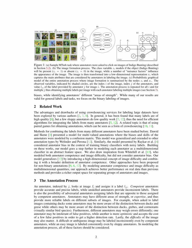
Figure 1: (a) Sample MTurk task where annotators were asked to click on images of Indigo Bunting (describedin Section 5.2). (b) The image formation process. The class variable zi models if the object (Indigo Bunting)will be present (zi = 1) or absent (zi = 0) in the image, while a number of “nuisance factors” influencethe appearance of the image. The image is then transformed into a low-dimensional representation xi whichcaptures the main attributes that are considered by annotators in labeling the image. (c) Probabilistic graphicalmodel of the entire annotation process where image formation is summarized by the nodes zi and xi. Theobserved variables, indicated by shaded circles, are the index i of the image, index j of the annotators, andvalue lij of the label provided by annotator j for image i. The annotation process is repeated for all i and formultiple j thus obtaining multiple labels per image with each annotator labeling multiple images (see Section 3).

biases, while identifying annotators’ different “areas of strength”. While many of our results arevalid for general labels and tasks, we focus on the binary labeling of images.

2 Related WorkThe advantages and drawbacks of using crowdsourcing services for labeling large datasets havebeen explored by various authors [2, 7, 8]. In general, it has been found that many labels are ofhigh quality [8], but a few sloppy annotators do low quality work [7, 12]; thus the need for efficientalgorithms for integrating the labels from many annotators [5, 12]. A related topic is that of usingpaired games for obtaining annotations, which can be seen as a form of crowdsourcing [10, 11].

Methods for combining the labels from many different annotators have been studied before. Dawidand Skene [1] presented a model for multi-valued annotations where the biases and skills of theannotators were modeled by a confusion matrix. This model was generalized and extended to otherannotation types by Welinder and Perona [12]. Similarly, the model presented by Raykar et al. [4]considered annotator bias in the context of training binary classifiers with noisy labels. Buildingon these works, our model goes a step further in modeling each annotator as a multidimensionalclassifier in an abstract feature space. We also draw inspiration from Whitehill et al. [13], whomodeled both annotator competence and image difficulty, but did not consider annotator bias. Ourmodel generalizes [13] by introducing a high-dimensional concept of image difficulty and combin-ing it with a broader definition of annotator competence. Other approaches have been proposedfor non-binary annotations [9, 6, 12]. By modeling annotator competence and image difficulty asmultidimensional quantities, our approach achieves better performance on real data than previousmethods and provides a richer output space for separating groups of annotators and images.

3 The Annotation ProcessAn annotator, indexed by j, looks at image Ii and assigns it a label lij . Competent annotatorsprovide accurate and precise labels, while unskilled annotators provide inconsistent labels. Thereis also the possibility of adversarial annotators assigning labels that are opposite to those assignedby competent annotators. Annotators may have different areas of strength, or expertise, and thusprovide more reliable labels on different subsets of images. For example, when asked to labelimages containing ducks some annotators may be more aware of the distinction between ducks andgeese while others may be more aware of the distinction between ducks, grebes, and cormorants(visually similar bird species). Furthermore, different annotators may weigh errors differently; oneannotator may be intolerant of false positives, while another is more optimistic and accepts the costof a few false positives in order to get a higher detection rate. Lastly, the difficulty of the imagemay also matter. A difficult or ambiguous image may be labeled inconsistently even by competentannotators, while an easy image is labeled consistently even by sloppy annotators. In modeling theannotation process, all of these factors should be considered.

2

We model the annotation process in a sequence of steps. N images are produced by some imagecapture/collection process. First, a variable zi decides which set of “objects” contribute to producingan image Ii. For example, zi ∈ {0, 1} may denote the presence/absence of a particular bird species.A number of “nuisance factors,” such as viewpoint and pose, determine the image (see Figure 1).

Each image is transformed by a deterministic “visual transformation” converting pixels into a vectorof task-specific measurements xi, representing measurements that are available to the visual systemof an ideal annotator. For example, the xi could be the firing rates of task-relevant neurons in thebrain of the best human annotator. Another way to think about xi is that it is a vector of visualattributes (beak shape, plumage color, tail length etc) that the annotator will consider when decidingon a label. The process of transforming zi to the “signal” xi is stochastic and it is parameterized byθz , which accounts for the variability in image formation due to the nuisance factors.

There are M annotators in total, and the set of annotators that label image i is denoted by Ji.An annotator j ∈ Ji, selected to label image Ii, does not have direct access to xi, but rather toyij = xi + nij , a version of the signal corrupted by annotator-specific and image-specific “noise”nij . The noise process models differences between the measurements that are ultimately availableto individual annotators. These differences may be due to visual acuity, attention, direction of gaze,etc. The statistics of this noise are different from annotator to annotator and are parametrized by σj .Most significantly, the variance of the noise will be lower for competent annotators, as they are morelikely to have access to a clearer and more consistent representation of the image than confused orunskilled annotators.

The vector yij can be understood as a perceptual encoding that encompasses all major componentsthat affect an annotator’s judgment on an annotation task. Each annotator is parameterized by a unitvector wj , which models the annotator’s individual weighting on each of these components. In thisway, wj encodes the training or expertise of the annotator in a multidimensional space. The scalarprojection 〈yij , wj〉 is compared to a threshold τj . If the signal is above the threshold, the annotatorassigns a label lij = 1, and lij = 0 otherwise.

4 Model and InferencePutting together the assumptions of the previous section, we obtain the graphical model shown inFigure 1. We will assume a Bayesian treatment, with priors on all parameters. The joint probabilitydistribution, excluding hyper-parameters for brevity, can be written as

p(L, z, x, y, σ, w, τ) =

M∏j=1

p(σj)p(τj)p(wj)

N∏i=1

p(zi)p(xi | zi) ∏j∈Ji

p(yij | xi, σj) p(lij | wj , τj , yij)

,

(1)where we denote z, x, y, σ, τ , w, and L to mean the sets of all the corresponding subscriptedvariables. This section describes further assumptions on the probability distributions. These as-sumptions are not necessary; however, in practice they simplify inference without compromisingthe quality of the parameter estimates.

Although both zi and lij may be continuous or multivalued discrete in a more general treatmentof the model [12], we henceforth assume that they are binary, i.e. zi, lij ∈ {0, 1}. We assume aBernoulli prior on zi with p(zi = 1) = β, and that xi is normally distributed1 with variance θ2z ,

p(xi | zi) = N (xi; µz, θ2z), (2)

where µz = −1 if zi = 0 and µz = 1 if zi = 1 (see Figure 2a). If xi and yij are multi-dimensional,then σj is a covariance matrix. These assumptions are equivalent to using a mixture of Gaussiansprior on xi.

The noisy version of the signal xi that annotator j sees, denoted by yij , is assumed to be generated bya Gaussian with variance σ2

j centered at xi, that is p(yij | xi, σj) = N (yij ; xi, σ2j ) (see Figure 2b).

We assume that each annotator assigns the label lij according to a linear classifier. The classifier isparameterized by a direction wj of a decision plane and a bias τj . The label lij is deterministicallychosen, i.e. lij = I (〈wj , yij〉 ≥ τj), where I (·) is the indicator function. It is possible to integrate

1We used the parameters β = 0.5 and θz = 0.8.

3

x1i

x2i

xi = (x1i , x

2i )

wj = (w1j , w2

j )τj

p(xi | zi = 0)

p(xi | zi = 1)

!3 !2 !1 0 1 2 3 !3 !2 !1 0 1 2 3

1 2 3 4 5 6 7 8

(a) (b) (c)p(yij | zi = 1)

p(yij | zi = 0)

xi

A

B

C

p(xi | zi = 0) p(xi | zi = 1)

p(y

ij|x

i)

τjτjyij yij

Figure 2: Assumptions of the model. (a) Labeling is modeled in a signal detection theory framework, wherethe signal yij that annotator j sees for image Ii is produced by one of two Gaussian distributions. Dependingon yij and annotator parameters wj and τj , the annotator labels 1 or 0. (b) The image representation xi isassumed to be generated by a Gaussian mixture model where zi selects the component. The figure shows 8different realizations xi (x1, . . . , x8), generated from the mixture model. Depending on the annotator j, noisenij is added to xi. The three lower plots shows the noise distributions for three different annotators (A,B,C),with increasing “incompetence” σj . The biases τj of the annotators are shown with the red bars. Image no. 4,represented by x4, is the most ambiguous image, as it is very close to the optimal decision plane at xi = 0. (c)An example of 2-dimensional xi. The red line shows the decision plane for one annotator.

out yij and put lij in direct dependence on xi,

p(lij = 1 | xi, σj , τj) = Φ

( 〈wj , xi〉 − τjσj

), (3)

where Φ(·) is the cumulative standardized normal distribution, a sigmoidal-shaped function.

In order to remove the constraint on wj being a direction, i.e. ‖wj‖2 = 1, we reparameterize theproblem with wj = wj/σj and τj = τj/σj . Furthermore, to regularize wj and τj during inference,we give them Gaussian priors parameterized by α and γ respectively. The prior on τj is centered atthe origin and is very broad (γ = 3). For the prior on wj , we kept the center close to the origin tobe initially pessimistic of the annotator competence, and to allow for adversarial annotators (mean1, std 3). All of the hyperparameters were chosen somewhat arbitrarily to define a scale for theparameter space, and in our experiments we found that results (such as error rates in Figure 3) werequite insensitive to variations in the hyperparameters. The modified Equation 1 becomes,

p(L, x, w, τ) =

M∏j=1

p(τj | γ)p(wj | α)

N∏i=1

p(xi | θz, β)∏j∈Ji

p(lij | xi, wj , τj)

. (4)

The only observed variables in the model are the labels L = {lij}, from which the other parametershave to be inferred. Since we have priors on the parameters, we proceed by MAP estimation, wherewe find the optimal parameters (x?, w?, τ?) by maximizing the posterior on the parameters,

(x?, w?, τ?) = arg maxx,w,τ

p(x,w, τ | L) = arg maxx,w,τ

m(x,w, τ), (5)

where we have defined m(x,w, τ) = log p(L, x, w, τ) from Equation 4. Thus, to do inference, weneed to optimize

m(x,w, τ) =

N∑i=1

log p(xi | θz, β) +

M∑j=1

log p(wj | α) +

M∑j=1

log p(τj | γ)

+

N∑i=1

∑j∈Ji

[lij log Φ (〈wj , xi〉 − τj) + (1− lij) log (1− Φ (〈wj , xi〉 − τj))] . (6)

To maximize (6) we carry out alternating optimization using gradient ascent. We begin by fixing thex parameters and optimizing Equation 6 for (w, τ) using gradient ascent. Then we fix (w, τ) andoptimize for x using gradient ascent, iterating between fixing the image parameters and annotatorparameters back and forth. Empirically, we have observed that this optimization scheme usuallyconverges within 20 iterations.

4

number of annotators number of annotators number of annotators number of annotators

Figure 3: (a) and (b) show the correlation between the ground truth and estimated parameters as the numberof annotators increases on synthetic data for 1-d and 2-d xi and wj . (c) Performance of our model in predictingzi on the data from (a), compared to majority voting, the model of [1], and GLAD [13]. (d) Performance onreal labels collected from MTurk. See Section 5.1 for details on (a-c) and Section 5.2 for details on (d).

In the derivation of the model above, there is no restriction on the dimensionality of xi and wj ;they may be one-dimensional scalars or higher-dimensional vectors. In the former case, assumingwj = 1, the model is equivalent to a standard signal detection theoretic model [3] where a signalyij is generated by one of two Normal distributions p(yij | zi) = N (yij | µz, s2) with variances2 = θ2z + σ2

j , centered on µ0 = −1 and µ1 = 1 for zi = 0 and zi = 1 respectively (see Figure 2a).In signal detection theory, the sensitivity index, conventionally denoted d′, is a measure of how wellthe annotator can discriminate the two values of zi [14]. It is defined as the Mahalanobis distancebetween µ0 and µ1 normalized by s,

d′ =µ1 − µ0

s=

2√θ2z + σ2

j

. (7)

Thus, the lower σj , the better the annotator can distinguish between classes of zi, and the more“competent” he is. The sensitivity index can also be computed directly from the false alarm rate fand hit rate h using d′ = Φ−1(h) − Φ−1(f) where Φ−1(·) is the inverse of the cumulative normaldistribution [14]. Similarly, the “threshold”, which is a measure of annotator bias, can be computedby λ = − 1

2

(Φ−1(h) + Φ−1(f)

). A large positive λ means that the annotator attributes a high cost

to false positives, while a large negative λmeans the annotator avoids false negative mistakes. Underthe assumptions of our model, λ is related to τj in our model by the relation λ = τj/s.

In the case of higher dimensional xi andwj , each component of the xi vector can be thought of as anattribute or a high level feature. For example, the task may be to label only images with a particularbird species, say “duck”, with label 1, and all other images with 0. Some images contain no birdsat all, while other images contain birds similar to ducks, such as geese or grebes. Some annotatorsmay be more aware of the distinction between ducks and geese and others may be more aware ofthe distinction between ducks, grebes and cormorants. In this case, xi can be considered to be 2-dimensional. One dimension represents image attributes that are useful in the distinction betweenducks and geese, and the other dimension models parameters that are useful in distinction betweenducks and grebes (see Figure 2c). Presumably all annotators see the same attributes, signified by xi,but they use them differently. The model can distinguish between annotators with preferences fordifferent attributes, as shown in Section 5.2.

Image difficulty is represented in the model by the value of xi (see Figure 2b). If there is a particularground truth decision plane, (w′, τ ′), images Ii with xi close to the plane will be more difficult forannotators to label. This is because the annotators see a noise corrupted version, yij , of xi. Howwell the annotators can label a particular image depends on both the closeness of xi to the groundtruth decision plane and the annotator’s “noise” level, σj . Of course, if the annotator bias τj is farfrom the ground truth decision plane, the labels for images near the ground truth decision plane willbe consistent for that annotator, but not necessarily correct.

5 Experiments5.1 Synthetic DataTo explore whether the inference procedure estimates image and annotator parameters accurately,we tested our model on synthetic data generated according to the model’s assumptions. Similar tothe experimental setup in [13], we generated 500 synthetic image parameters and simulated between4 and 20 annotators labeling each image. The procedure was repeated 40 times to reduce the noisein the results.

We generated the annotator parameters by randomly sampling σj from a Gamma distribution (shape1.5 and scale 0.3) and biases τj from a Normal distribution centered at 0 with standard deviation

5

(a) (b) (c) (d)

Figure 4: Ellipse dataset. (a) The images to be labeled were fuzzy ellipses (oriented uniformly from 0 to π)enclosed in dark circles. The task was to select ellipses that were more vertical than horizontal (the former aremarked with green circles in the figure). (b-d) The image difficulty parameters xi, annotator competence 2/s,and bias τj/s learned by our model are compared to the ground truth equivalents. The closer xi is to 0, themore ambiguous/difficult the discrimination task, corresponding to ellipses that have close to 45◦ orientation.

0.5. The direction of the decision plane wj was +1 with probability 0.99 and −1 with probability0.01. The image parameters xi were generated by a two-dimensional Gaussian mixture model withtwo components of standard deviation 0.8 centered at -1 and +1. The image ground truth labelzi, and thus the mixture component from which xi was generated, was sampled from a Bernoullidistribution with p(zi = 1) = 0.5.

For each trial, we measured the correlation between the ground truth values of each parameter andthe values estimated by the model. We averaged Spearman’s rank correlation coefficient for eachparameter over all trials. The result of the simulated labeling process is shown Figure 3a. As canbe seen from the figure, the model estimates the parameters accurately, with the accuracy increasingas the number of annotators labeling each image increases. We repeated a similar experiment with2-dimensional xi and wj (see Figure 3b). As one would expect, estimating higher dimensional xiand wj requires more data.

We also examined how well our model estimated the binary class values, zi. For comparison, we alsotried three other methods on the same data: a simple majority voting rule for each image, the bias-competence model of [1], and the GLAD algorithm from [13]2, which models 1-d image difficultyand annotator competence, but not bias. As can be seen from Figure 3c, our method presents a smallbut consistent improvement. In a separate experiment (not shown) we generated synthetic annotatorswith increasing bias parameters τj . We found that GLAD performs worse than majority voting whenthe variance in the bias between different annotators is high (γ & 0.8); this was expected as GLADdoes not model annotator bias. Similarly, increasing the proportion of difficult images degrades theperformance of the model from [1]. The performance of our model points to the benefits of modelingall aspects of the annotation process.

5.2 Human DataWe next conducted experiments on annotation results from real MTurk annotators. To compare theperformance of the different models on a real discrimination task, we prepared dataset of 200 imagesof birds (100 with Indigo Bunting, and 100 with Blue Grosbeak), and asked 40 annotators per imageif it contained at least one Indigo Bunting; this is a challenging task (see Figure 1). The annotatorswere given a description and example photos of the two bird species. Figure 3d shows how theperformance varies as the number of annotators per image is increased. We sampled a subset of theannotators for each image. Our model did better than the other approaches also on this dataset.

To demonstrate that annotator competence, annotator bias, image difficulty, and multi-dimensionaldecision surfaces are important real life phenomena affecting the annotation process, and to quantifyour model’s ability to adapt to each of them, we tested our model on three different image datasets:one based on pictures of rotated ellipses, another based on synthetically generated “greebles”, and athird dataset with images of waterbirds.

Ellipse Dataset: Annotators were given the simple task of selecting ellipses which they believedto be more vertical than horizontal. This dataset was chosen to make the model’s predictions quan-

2We used the implementation of GLAD available on the first author’s website: http://mplab.ucsd.edu/˜jake/

We varied the α prior in their code between 1-10 to achieve best performance.

6

E

F

G

H

A

B

C

Dx1

i

x2i

Figure 5: Estimated image parameters (symbols) and annotator decision planes (lines) for the greeble ex-periment. Our model learns two image parameter dimensions x1i and x2i which roughly correspond to colorand height, and identifies two clusters of annotator decision planes, which correctly correspond to annotatorsprimed with color information (green lines) and height information (red lines). On the left are example imagesof class 1, which are shorter and more yellow (red and blue dots are uncorrelated with class), and on the rightare images of class 2, which are taller and more green. C and F are easy for all annotators, A and H aredifficult for annotators that prefer height but easy for annotators that prefer color, D and E are difficult forannotators that prefer color but easy for annotators that prefer height, B and G are difficult for all annotators.

tifiable, because ground truth class labels and ellipse angle parameters are known to us for each testimage (but hidden from the inference algorithm).

By definition, ellipses at an angle of 45◦ are impossible to classify, and we expect that imagesgradually become easier to classify as the angle moves away from 45◦. We used a total of 180 ellipseimages, with rotation angle varying from 1-180◦, and collected labels from 20 MTurk annotators foreach image. In this dataset, the estimated image parameters xi and annotator parameters wj are 1-dimensional, where the magnitudes encode image difficulty and annotator competence respectively.Since we had ground truth labels, we could compute the false alarm and hit rates for each annotator,and thus compute λ and d′ for comparison with τj/s and 2/s (see Equation 7 and following text).

The results in Figure 4b-d show that annotator competence and bias vary among annotators. More-over, the figure shows that our model accurately estimates image difficulty, annotator competence,and annotator bias on data from real MTurk annotators.

Greeble Dataset: In the second experiment, annotators were shown pictures of “greebles” (seeFigure 5) and were told that the greebles belonged to one of two classes. Some annotators weretold that the two greeble classes could be discriminated by height, while others were told they couldbe discriminated by color (yellowish vs. green). This was done to explore the scenario in whichannotators have different types of prior knowledge or abilities. We used a total of 200 images with20 annotators labeling each image. The height and color parameters for the two types of greebleswere randomly generated according to Gaussian distributions with centers (1, 1) and (−1,−1), andstandard deviations of 0.8.

The results in Figure 5 show that the model successfully learned two clusters of annotator decisionsurfaces, one (green) of which responds mostly to the first dimension of xi (color) and another (red)responding mostly to the second dimension of xi (height). These two clusters coincide with thesets of annotators primed with the two different attributes. Additionally, for the second attribute, weobserved a few “adversarial” annotators whose labels tended to be inverted from their true values.This was because the instructions to our color annotation task were ambiguously worded, so thatsome annotators had become confused and had inverted their labels. Our model robustly handlesthese adversarial labels by inverting the sign of the w vector.

Waterbird Dataset: The greeble experiment shows that our model is able to segregate annotatorslooking for different attributes in images. To see whether the same phenomenon could be observed ina task involving images of real objects, we constructed an image dataset of waterbirds. We collected50 photographs each of the bird species Mallard, American Black Duck, Canada Goose and Red-necked Grebe. In addition to the 200 images of waterbirds, we also selected 40 images without anybirds at all (such as photos of various nature scenes and objects) or where birds were too small beseen clearly, making 240 images in total. For each image, we asked 40 annotators on MTurk if theycould see a duck in the image (only Mallards and American Black Ducks are ducks). The hypothesis

7

1

2

3

x1i

x2i

Figure 6: Estimated image and annotator parameters on the Waterbirds dataset. The annotators were askedto select images containing at least one “duck”. The estimated xi parameters for each image are marked withsymbols that are specific to the class the image belongs to. The arrows show the xi coordinates of some exampleimages. The gray lines are the decision planes of the annotators. The darkness of the lines is an indicator of‖wj‖: darker gray means the model estimated the annotator to be more competent. Notice how the annotators’decision planes fall roughly into three clusters, marked by the blue circles and discussed in Section 5.2.

was that some annotators would be able to discriminate ducks from the two other bird species, whileothers would confuse ducks with geese and/or grebes.

Results from the experiment, shown in Figure 6, suggest that there are at least three different groupsof annotators, those who separate: (1) ducks from everything else, (2) ducks and grebes from every-thing else, and (3) ducks, grebes, and geese from everything else; see numbered circles in Figure 6.Interestingly, the first group of annotators was better at separating out Canada geese than Red-neckedgrebes. This may be because Canada geese are quite distinctive with their long, black necks, whilethe grebes have shorter necks and look more duck-like in most poses. There were also a few outlierannotators that did not provide answers consistent with any other annotators. This is a commonphenomenon on MTurk, where a small percentage of the annotators will provide bad quality labelsin the hope of still getting paid [7]. We also compared the labels predicted by the different modelsto the ground truth. Majority voting performed at 68.3% correct labels, GLAD at 60.4%, and ourmodel performed at 75.4%.

6 ConclusionsWe have proposed a Bayesian generative probabilistic model for the annotation process. Givenonly binary labels of images from many different annotators, it is possible to infer not only theunderlying class (or value) of the image, but also parameters such as image difficulty and annota-tor competence and bias. Furthermore, the model represents both the images and the annotatorsas multidimensional entities, with different high level attributes and strengths respectively. Experi-ments with images annotated by MTurk workers show that indeed different annotators have variablecompetence level and widely different biases, and that the annotators’ classification criterion is bestmodeled in multidimensional space. Ultimately, our model can accurately estimate the ground truthlabels by integrating the labels provided by several annotators with different skills, and it does sobetter than the current state of the art methods.

Besides estimating ground truth classes from binary labels, our model provides information that isvaluable for defining loss functions and for training classifiers. For example, the image parame-ters estimated by our model could be taken into account for weighing different training examples,or, more generally, it could be used for a softer definition of ground truth. Furthermore, our find-ings suggest that annotators fall into different groups depending on their expertise and on how theyperceive the task. This could be used to select annotators that are experts on certain tasks and todiscover different schools of thought on how to carry out a given task.

Acknowledgements

P.P. and P.W. were supported by ONR MURI Grant #N00014-06-1-0734 and EVOLUT.ONR2. S.B. was sup-ported by NSF CAREER Grant #0448615, NSF Grant AGS-0941760, ONR MURI Grant #N00014-08-1-0638,and a Google Research Award.

8

References

[1] A. P. Dawid and A. M. Skene. Maximum likelihood estimation of observer error-rates usingthe em algorithm. J. Roy. Statistical Society, Series C, 28(1):20–28, 1979. 1, 2, 5, 6

[2] J. Deng, W. Dong, R. Socher, L.-J. Li, K. Li, and L. Fei-Fei. ImageNet: A Large-ScaleHierarchical Image Database. In CVPR, 2009. 2

[3] D.M. Green and J.M. Swets. Signal detection theory and psychophysics. John Wiley and SonsInc, New York, 1966. 5

[4] V.C. Raykar, S. Yu, L.H. Zhao, A. Jerebko, C. Florin, G.H. Valadez, L. Bogoni, and L. Moy.Supervised Learning from Multiple Experts: Whom to trust when everyone lies a bit. In ICML,2009. 1, 2

[5] V.S. Sheng, F. Provost, and P.G. Ipeirotis. Get another label? improving data quality and datamining using multiple, noisy labelers. In KDD, 2008. 1, 2

[6] P. Smyth, U. Fayyad, M. Burl, P. Perona, and P. Baldi. Inferring ground truth from subjectivelabelling of Venus images. NIPS, 1995. 1, 2

[7] R. Snow, B. O’Connor, D. Jurafsky, and A.Y. Ng. Cheap and Fast - But is it Good? EvaluatingNon-Expert Annotations for Natural Language Tasks. In EMNLP, 2008. 1, 2, 8

[8] A. Sorokin and D. Forsyth. Utility data annotation with amazon mechanical turk. In FirstIEEE Workshop on Internet Vision at CVPR’08, 2008. 1, 2

[9] M. Spain and P. Perona. Some objects are more equal than others: measuring and predictingimportance. In ECCV, 2008. 1, 2

[10] L. von Ahn and L. Dabbish. Labeling images with a computer game. In SIGCHI conferenceon Human factors in computing systems, pages 319–326, 2004. 2

[11] L. von Ahn, B. Maurer, C. McMillen, D. Abraham, and M. Blum. reCAPTCHA: Human-basedcharacter recognition via web security measures. Science, 321(5895):1465–1468, 2008. 2

[12] Peter Welinder and Pietro Perona. Online crowdsourcing: rating annotators and obtaining cost-effective labels. In IEEE Conference on Computer Vision and Pattern Recognition Workshops(ACVHL), 2010. 1, 2, 3

[13] J. Whitehill, P. Ruvolo, T. Wu, J. Bergsma, and J. Movellan. Whose vote should count more:Optimal integration of labels from labelers of unknown expertise. In NIPS, 2009. 1, 2, 5, 6

[14] T. D. Wickens. Elementary signal detection theory. Oxford University Press, United States,2002. 5

9