Queueing Syst (2015) 79:391–426DOI 10.1007/s11134-014-9429-3

Stochastic grey-box modeling of queueing systems:fitting birth-and-death processes to data

James Dong · Ward Whitt

Received: 8 January 2014 / Revised: 17 November 2014 / Published online: 2 December 2014© Springer Science+Business Media New York 2014

Abstract This paper explores grey-box modeling of queueing systems. A stationarybirth-and-death (BD) process model is fitted to a segment of the sample path of thenumber in the system in the usual way. The birth (death) rates in each state are estimatedby the observed number of arrivals (departures) in that state divided by the total timespent in that state. Under minor regularity conditions, if the queue length (number in thesystem) has a proper limiting steady-state distribution, then the fitted BD process hasthat same steady-state distribution asymptotically as the sample size increases, evenif the actual queue-length process is not nearly a BD process. However, the transientbehavior may be very different. We investigate what we can learn about the actualqueueing system from the fitted BD process. Here we consider the standard G I/G I/squeueing model with s servers, unlimited waiting room and general independent,non-exponential, interarrival-time and service-time distributions. For heavily loadeds-server models, we find that the long-term transient behavior of the original process,as partially characterized by mean first passage times, can be approximated by adeterministic time transformation of the fitted BD process, exploiting the heavy-trafficcharacterization of the variability.

J. DongSchool of Operations Research and Information Engineering, Cornell University,287 Rhodes Hall, Ithaca, NY 14850, USAe-mail: jd748@cornell.edu

W. Whitt (B)Department of Industrial Engineering and Operations Research,Columbia University, New York, NY 10027, USAe-mail: ww2040@columbia.edu

123

392 Queueing Syst (2015) 79:391–426

Keywords Birth-and-death processes · Grey-box modeling · Fitting stochasticmodels to data · Transient behavior · First passage times · Heavy traffic

Mathematics Subject Classification 60F17 · 60J25 · 60K25 · 62M09 · 90B25

1 Introduction

Queueing theory primarily involves white-box modeling, in which queueing modelsare defined from first principles and analyzed. To apply these models to analyze theperformance of queueing systems, we check that the assumptions of the models aresatisfied, for example, by performing statistical tests on system data, as in [7,28], andestimating model parameters, as in [4,5,36] and references therein.

An alternative to white-box modeling of queueing systems is black-box modeling,in which models (for example, statistical time-series methods) are employed, withoutusing any structure of queueing models; see [42,59]. Black-box modeling is growing inpopularity as the amount of available data grows, as well as our ability to extract usefulinformation from it; see [22]. A modeling approach in between these two extremes,which might conceivably share the advantages of both, is grey-box modeling, whichexploits some model structure together with learning from data; see [6,29].

We examine grey-box modeling applied to queueing processes. In this paper, thegrey-box model is a general stationary birth-and-death (BD) process, which exploitsthe common property of many queue-length (number in system) processes that theyalmost surely make only unit transitions, corresponding to separate arrivals and depar-tures. Indeed, BD queueing models such as the Markovian M/M/s model are wellstudied and have been extensively used. Moreover, BD models have been found to beuseful approximations for other more general but less tractable models, as illustratedby the BD approximation in [52] for the M/G I/s +G I model having customer aban-donment from the queue with non-exponential patience times (the +G I ) as well asnon-exponential service times.

The main idea here is to approach an application where we do not know whatmodel is appropriate by fitting a stationary BD process to an observed segment of thesample path of a queue-length stochastic process, assuming only that it increases anddecreases in unit steps. Just as is commonly done for estimating rates in a BD process[5,26,57], we estimate the birth rate in state k from arrival data over an interval [0, t]by λk ≡ λk(t), the number of arrivals observed in that state, divided by the totaltime spent in that state, while we estimate the death rate in state k by μk ≡ μk(t),the number of departures observed in that state, divided by the total time spent inthat state. As usual, the steady-state distribution of that fitted BD model, denoted byαe

k ≡ αek(t) (with superscript e indicating the estimated rates), is well defined (under

regularity conditions, see [54]) and is characterized as the unique probability vectorsatisfying the local balance equations,

αek λk = αe

k+1μk+1, k ≥ 0. (1.1)

Throughout this paper, we assume that limiting values of the rates as t → ∞ existand that our estimators are consistent, so we omit the t .

123

Queueing Syst (2015) 79:391–426 393

The BD process is appealing as a grey-box model for queueing systems, because thefitted BD steady-state distribution {αe

k : k ≥ 0} in (1.1) closely matches the empiricalsteady-state distribution, {αk : k ≥ 0}, where αk ≡ αk(t) is the proportion of totaltime spent in each state. Indeed, as has been known for some time (for example,see Chapter 4 of [19]), under regularity conditions, these two distributions coincideasymptotically as t (and thus the sample size) increases, even if the actual systemevolves in a very different way from the fitted BD process. For example, the actualprocess {Q(t) : t ≥ 0} might be periodic or non-Markovian; see [46].

If we directly fit a BD process to data as just described, we should not concludewithout further testing that the underlying queue-length process actually is a BDprocess. In fact, the main point of [54] was to caution against drawing unwarrantedpositive conclusions from a close similarity in the steady-state distributions, becausethese two distributions are automatically closely related. Nevertheless, the fitted BDprocess might provide useful insight about the underlying system. The purpose of thepresent paper is to start investigating that idea.

In fact, our earlier paper [54] was largely motivated by exploratory data analysiscarried out in Sect. 3 of [3]. They had fitted several candidate models to data on thenumber of patients in a hospital emergency department, and found that a BD processfit better than others. After writing our previous paper [54], cautioning against drawingunwarranted positive conclusions, we realized that fitting BD processes to data mightindeed be useful, and started the present investigation. See Sect. 3 of [3] for morediscussion about exploratory data analysis of an emergency department.

There also is a much earlier precedent for exploiting fitted BD processes. This ideawas part of the program of operational analysis suggested by Buzen and Denning[8,9,15] in early performance analysis of computer systems. However, they expressedthe view that there was no need for an associated “underlying” stochastic model. Incontrast, as in Sects. 4.6–4.7 of [19], we think that an underlying stochastic modelshould play an important role. With that in mind, we want to see if the fitted BD modelcan provide useful insight into an unknown underlying stochastic model.

Our goal in the present paper is to better understand this fitted BD model. Weprimarily want to answer two questions:

(i) How are the fitted birth and death rates related to the key structural features ofan actual queueing model?

(ii) How does the transient behavior of an actual queueing system differ from thetransient behavior of the fitted BD process?

We start to address the first question by estimating the birth and death rates fromsimulation experiments for G I/G I/s models. When the interarrival-time (service-time) distribution is exponential, then the fitted birth (death) rate captures the truebehavior of the queue-length process, but otherwise it does not. For non-exponentialdistributions, we see that the fitted rates evidently have substantial structure, whichwe do our best to explain.

We start to address the second question by looking at first passage times in theunderlying model and the fitted model. Perhaps our most interesting finding is a simpleconnection between the fitted BD process Qf ≡ {Qf(t) : t ≥ 0} and the queue-length (number in system) process Q ≡ {Q(t) : t ≥ 0} for a stationary G I/G I/s

123

394 Queueing Syst (2015) 79:391–426

model, which holds approximately under two conditions: (i) if we focus on the long-term transient behavior, as measured by the expected first passage time from the pth

percentile of the stationary distribution to the (1 − p)th percentile and back again forp suitably small, for example, p = 0.1, and (ii) if we consider models with relativelyhigh traffic intensity, so that heavy-traffic approximations are appropriate. Under thesetwo conditions, we find that the two processes differ primarily in a one-dimensionalway, by the speed that they move through the state space. In other words, we suggestthe process approximation

{Q(t) : t ≥ 0} ≈ {Qf(t/ω) : t ≥ 0}, (1.2)

where ω is the speed ratio, which admits the conventional heavy-traffic approximation(traffic intensity ρ near 1 with finitely many servers)

ω ≈ c2a + c2

s

2, (1.3)

with c2a and c2

s being the squared coefficients of variation (scv’s, variance divided bythe square of the mean) of an interarrival time and a service time, respectively; seeTables 2, 3, 4, and 5. The approximating speed ratio in (1.3) can be recognized asthe heavy-traffic characterization of the variability in the G I/G I/s queueing model.We also discuss how to estimate the speed ratio in s-server models without the strongindependent assumptions; see Sect. 7.1.

We provide important mathematical support for (1.2) with (1.3) for both theG I/G I/s model in the conventional heavy-traffic regime by Corollaries 5.1 and 5.2(and the results leading up to them) and for the G I/M/∞ model in the many-serverheavy-traffic regime by Corollary 6.2 (and the results leading up to it). These corol-laries establish that (1.2) with (1.3) is asymptotically correct in a heavy-traffic limitin considerable generality. In order to establish these results, we have to make quitestrong assumptions on the fitted birth rates (consistent with our simulation results),but we conjecture that these properties of the fitted rates hold; see Conjectures 2.1, 2.2and 5.1. The current conventional heavy-traffic results fully cover the G I/M/s modelby virtue of Theorem 3.1.

The proofs of these heavy-traffic limits are interesting because they depend on dif-ferences in the stochastic-process limits for the original queue-length process and thefitted BD process. The two processes necessarily have the same steady-state distribu-tion, as we observed above. Since both processes are asymptotically characterized bydiffusion limits, we see that the common steady-state distribution is achieved by thenon-Markov variability captured by the diffusion coefficient in the diffusion approx-imation for the original process being transferred into the drift of the diffusion limitof the fitted BD process. The fitted BD process evidently captures less of the localvariability in the original process. As a consequence, we get the speed ratio as in (1.2)above.

Consistent with extensive experience about the many-server heavy-traffic regime,we also discover that a very different story holds for large-scale many-server queue-ing systems with non-exponential service-time distributions, where the very different

123

Queueing Syst (2015) 79:391–426 395

many-server heavy-traffic approximations are appropriate. In particular, we find thatthe approximation in (1.2) is still appropriate for other G I/G I/∞ models withnon-exponential service-time distributions, but that (1.3) is not appropriate. Indeed,the speed ratio in the M/G I/∞ model tends to depend on the scv c2

s of the non-exponential service-time distribution in way that is inversely related to (1.3); seeTable 5.

Organization: We start in Sect. 2 by showing simulation estimates of the birthand death rates in G I/G I/1 single-server and G I/G I/s multi-server models fors = 40 and s = ∞, for various interarrival-time and service-time distributions.Next, in Sect. 3 we establish mathematical results showing how the fitted BD ratesdepend on the model structure of stable G I/G I/s models, trying to explain as muchas we can of the structure we see in the fitted rates. In Sect. 4 we define the speedratios in terms of first passage times and show simulation results for the speed ratio.Then in Sect. 5 we obtain insights about the fitted BD process and the speed ratioby making connections to conventional heavy-traffic limit theory. In Sect. 6 we makecorresponding connections to the many-server heavy-traffic theory. In Sect. 7 we dis-cuss estimation procedures. In Sect. 7.1 we discuss how to estimate the speed ratios,pointing out the possibility of exploiting indices of dispersion. In Sect. 7.2 we discusshow to estimate the birth and death rates, pointing out the advantages of smoothing.Finally, in Sect. 8 we draw conclusions. Additional details are provided in a shortAppendix.

2 Fitted rates in simulation experiments

We start by reporting results of simulation experiments for G I/G I/s models. Forthe non-exponential distributions, we use Erlang (Ek , sums of k i.i.d. exponentialswith c2 = 1/k, focusing on k = 2 and k = 4) and hyperexponential (H2(c2),mixtures of two i.i.d. exponentials with scv c2 > 1) to illustrate non-exponentialdistributions less and more variable than exponential. An H2 cdf can be expressed asF(x) ≡ p1(1−e−λ1x )+ p2(1−e−λ2x ). We fix one of the three parameters by assumingbalanced means, p1/λ1 = p2/λ2, as on p. 137 of [44]. We primarily consider H2(2)

with scv c2 = 2.For these models, it can be shown that the fitted rates are consistent estimators of

finite limiting values; i.e., λk(t) → λk , k ≥ 0, and μk(t) → μk , k ≥ 1, as t → ∞.(Justification can be by an application of the law of large numbers for renewal rewardprocesses, as in Ch. 3 of [37]; arrivals to an empty system can be the renewal epochs.)We assume that the t in question is sufficiently large that we can regard our estimateas the limiting value. We estimated the rates from 30 independent replications of 1million customers. This large sample size is sufficient for 95 % confidence intervalsof the state-dependent rates to be within 1 % of the rates for states k with steady-stateprobability αk ≥ 0.01. The width of the confidence intervals increases as a functionof the variability parameters c2

a and c2s . Of course, even though our simulation runs

are long, good estimates of the rates are only possible for states k that are frequentlyvisited.

123

396 Queueing Syst (2015) 79:391–426

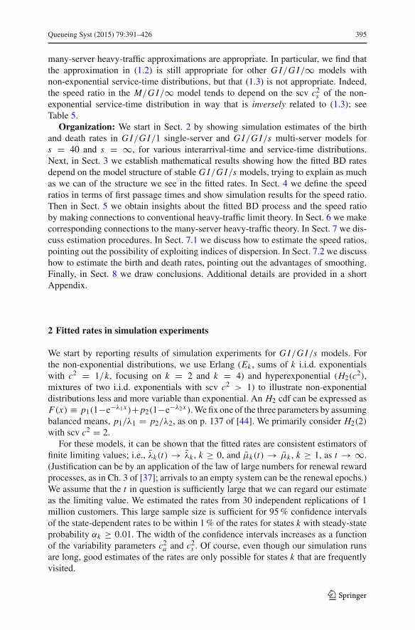
Fig. 1 Fitted birth rates λk (left) and death rates μk (right) for seven G I/G I/1 models with ρ = λ = 0.8and μ = 1

2.1 Single-server queues

We first fit birth rates and death rates to data from simulations of various G I/G I/1single-server models, all with traffic intensity ρ = 0.8. We let the mean service timebe 1/μ = 1 in all cases, so that the overall arrival rate is λ = ρ = 0.8. Fig. 1 showsthe fitted birth rates (left) and death rates (right) for seven different models. Some lossof statistical precision is seen in some of the plots for large values around k = 30 atthe right end of these plots.

From Fig. 1, the fitted rates seem to satisfy, at least approximately, the property

λk = λ and μk = μ for all k ≥ k0, (2.1)

for some k0, for example, k0 = 5. We show that the relations in (2.1) hold exactly inthe G I/M/s model (Theorem 3.1). We show that the fitted death rates differ in theM/G I/1 model for any two different service-time distributions (Theorem 3.3). Thus,the relation (2.1) evidently does not hold exactly for any non-exponential distributionin the M/G I/1 model. Evidently limits exist as k → ∞ for a large class of models.

We can make inferences about the interarrival-time and service-time distributionsfrom Fig. 1. First, from the queue-length sample path we can also estimate the arrivalrate λ and the service rate μ, which of course are known in advance in the simulationexperiments. Our estimated arrival (service) rate is A(t)/t (D(t)/B(t)), where A(t)(D(t)) is the total number of arrivals (departures) over the interval [0, t] (with D(t) ≈A(t) if t is large) and B(t) is the total time that the server is busy in [0, t].

Of particular importance for understanding performance is the fitted traffic inten-sity ρ ≡ λ/μ, which we would estimate or calculate directly as the limit ofρk ≡ λk/μk+1 = αk+1/αk as k → ∞; see Sect. 3.3. For its impact on congestion,we would focus on (1 − ρ)−1 and its relation to (1 − ρ)−1 via ω ≡ (1 − ρ)/(1 − ρ).An important observation is that all these quantities—λ, μ, ρ, and ω—are actuallyfunctions of ρ. Theorems 3.5 and 5.1 show that for a large class of G I/G I/s models

ω(ρ) ≡ 1 − ρ

1 − ρ(ρ)≈ ω ≡ c2

a + c2s

2(2.2)

123

Queueing Syst (2015) 79:391–426 397

Table 1 Estimates of the asymptotic fitted birth rate λ, death rate μ, traffic intensity ρ, and speed ratio ω

via (2.2) for the nine G I/G I/1 models with ρ = 0.8 in Fig. 1

Model λ μ ρ ω ω ≡ (c2a + c2

s )/2

E2/E2/1 0.700 ± 0.002 1.138 ± 0.026 0.603 ± 0.044 0.520 ± 0.035 0.500

E2/M/1 0.741 ± 0.001 1.002 ± 0.003 0.740 ± 0.001 0.770 ± 0.004 0.750

E2/H2(2)/1 0.766 ± 0.001 0.910 ± 0.001 0.843 ± 0.001 1.271 ± 0.010 1.250

M/E2/1 0.801 ± 0.001 1.074 ± 0.002 0.746 ± 0.003 0.788 ± 0.008 0.750

M/M/1 0.800 ± 0.001 1.000 ± 0.001 0.800 ± 0.002 1.000 ± 0.011 1.000

M/H2(2)/1 0.799 ± 0.001 0.926 ± 0.002 0.865 ± 0.001 1.478 ± 0.014 1.500

H2(2)/E2/1 0.867 ± 0.001 1.047 ± 0.001 0.828 ± 0.001 1.161 ± 0.009 1.250

H2(2)/M/1 0.857 ± 0.001 0.945 ± 0.003 0.857 ± 0.001 1.399 ± 0.011 1.500

H2(2)/H2(2)/1 0.843 ± 0.001 0.945 ± 0.003 0.893 ± 0.002 1.877 ± 0.027 2.000

when ρ is not too small, where ω is the theoretical speed ratio in (1.3).Table 1 shows the estimates of the asymptotic BD rates λ and μ with 95 % con-

fidence intervals and the associated estimates of the fitted traffic intensity ρ and thespeed ratio ω for the models with ρ = 0.8 in Fig. 1. This last estimate is comparedto the approximation in (2.2). These statistical estimates are obtained directly fromthe final estimated rates λk and μk by treating the values with 5 ≤ k ≤ 24 as asample from 20 i.i.d. normally distributed random variables with unknown variance,so that the confidence intervals are constructed with the Student t distribution having19 degrees of freedom. Of course, in this case the statistical precision is compoundedwith the actual deterministic variation in the rates, but Table 1 shows that both sourcesof variability are not great.

Figure 1 and Table 1 show that λ (μ) is increasing in c2a (c2

s ) with λ = λ (μ = μ) inthe M case when c2

a = 1 (c2s = 1). We provide theoretical support for this conclusion

in the G I/M/s model in Theorem 3.2. The last two columns of Table 1 provide supportfor the approximation in (2.2). The analogs of Fig. 1 and Table 1 for ρ = 0.9 are givenin the Appendix.

2.2 Many-server models

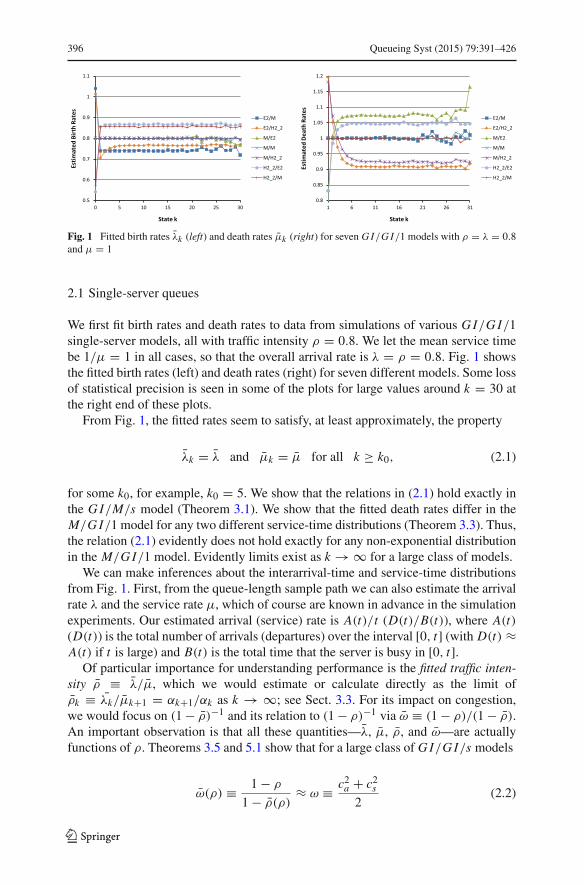
We next look at many-server models. Specifically, we consider seven G I/G I/s modelswith s = 40 and seven G I/G I/∞ models. These all have the parameters λ = 39 andμ = 1. The fitted birth and death rates are shown in Figs. 2 and 3. By Little’s law,the mean number of busy servers is always ρ ≡ λ/μ = 39. Since the number in thesystem tends to concentrate in the interval [20, 60], we show only that part. We wouldsee the impact of unreliable estimation outside of that interval.

The most striking behavior in Figs. 2 and 3 is the systematic structure of the deathrates within the interval [20, 60] of frequently visited states. We evidently have, atleast approximately,

μk = (k ∧ s)μ = (k ∧ s), k ≥ 1, (2.3)

123

398 Queueing Syst (2015) 79:391–426

Fig. 2 Fitted birth and death rates for seven G/G/40 models with λ = 39 and μ = 1

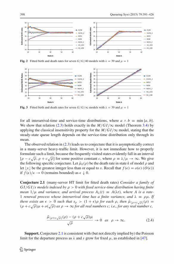
Fig. 3 Fitted birth and death rates for seven G/G/∞ models with λ = 39 and μ = 1

for all interarrival-time and service-time distributions, where a ∧ b ≡ min {a, b}.We show that relation (2.3) holds exactly in the M/G I/∞ model (Theorem 3.4) byapplying the classical insensitivity property for the M/G I/∞ model, stating that thesteady-state queue length depends on the service-time distribution only through itsmean.

The observed relation in (2.3) leads us to conjecture that it is asymptotically correctin a many-server heavy-traffic limit. However, it is not immediate how to properlyformulate such a limit, because the frequently visited states evidently fall in an interval[ρ − c

√ρ, ρ + c

√ρ] for some positive constant c, where ρ ≡ λ/μ → ∞. We give

the following specific conjecture. Let μk(ρ) be the death rate in state k of model ρ andlet x� be the greatest integer less than or equal to x . Recall that f (ε) = o(ε) (O(ε))if f (ε)/ε → 0 (remains bounded) as ε ↓ 0.

Conjecture 2.1 (many-server HT limit for fitted death rates) Consider a family ofG I/G I/s models indexed by ρ > 0 with fixed service-time distribution having finitemean 1/μ and variance, and arrival process Aλ(t) ≡ A(λt), where A is a rate-1 renewal process whose interarrival time has a finite variance, and λ ≡ ρμ. Ifthere exists an ε > 0 such that sρ > (1 + ε)ρ for each ρ, then μρ+c

√ρ�(ρ) =

(ρ + c√

ρ)μ + o(√

ρ) as ρ → ∞ for all real numbers c; i.e., for any real number c,

μρ+c√

ρ�(ρ) − (ρ + c√

ρ)μ√ρ

→ 0 as ρ → ∞. (2.4)

Support. Conjecture 2.1 is consistent with (but not directly implied by) the Poissonlimit for the departure process as λ and s grow for fixed μ, as established in [47].

123

Queueing Syst (2015) 79:391–426 399

Figure 3 also shows regularity in the arrival rates in infinite-server models. Forinfinite-server models with individual service rate μ = 1 and arrival rate ρ, we seethat, again at least approximately, the fitted birth rate in state k is

λρ,k ≡ 0 ∨ [ρ + b(k − ρ)], k ≥ 0, (2.5)

where the constant b depends on the interarrival-time distribution, satisfying −∞ <

b < 1, and a ∨ b ≡ max {a, b}. (The maximum is needed to prevent the arrival ratefrom becoming negative as k increases if b < 0.)

Paralleling Conjecture 2.1, we conjecture that the conclusions of (2.5) hold moregenerally.

Conjecture 2.2 (HT limit for fitted arrival rates in infinite-server models) In additionto Conjecture 2.1, for G I/G I/∞ infinite-server models,

λρ,k − 0 ∨ [ρ + b(k − ρ)]√ρ

→ 0 as ρ → ∞ (2.6)

for all integers k.

Formula 2.5 holds exactly with b = 0 for exponential interarrival times; otherwiseFig. 3 shows that b > (<)0 when c2

a > (<)1. Formula (2.5) also is appropriate fork ≤ s in s-server systems provided that s is suitably large, at least s > n, as in Fig. 2.

2.3 Detecting deviations from the G I/G I/s model

In applications, estimating birth and death rates may be especially useful to detectdeviations from the G I/G I/s model. Figs. 1 and 2 suggest that such deviations maybe easy to detect, because these figures show remarkable consistency in the estimatedbirth and death rates. For states k > s, the rates are nearly constant in all cases. Weshould thus be able to detect model deviations in which customers are less likelyto join if there is a long queue (causing birth rates to decrease in k) or impatientcustomers abandon the queue (causing death rates to increase in k) as k increasesabove s. A specific model with these features is the modification of the M/M/s queuewith state-dependent balking and abandonment, having parameters

λk ≡ λe−(k−s)+ and μk ≡ μ(k ∧ s) + θ(k − s)+, k ≥ 0. (2.7)

where (x)+ ≡ max {x, 0}. Figures 1 and 2 show that those effects are highly unlikelyto be caused by just having a G I/G I/s model with non-exponential distributions.

The consistent piecewise-linear structure for larger s in Fig. 2 shows that we shouldbe able to detect if the actual number of servers varies over time, as in [53]. Forexample, if there were s1 servers over the interval [0, t/2) and s2 servers over theinterval [t/2, t], where s1 < s2, then we would have the average of two of the plotsin Fig. 2. Unlike Fig. 2, the estimated birth and death rates would have three separatelinear pieces, over the intervals [0, s1], [s1, s2], and [s2,∞).

123

400 Queueing Syst (2015) 79:391–426

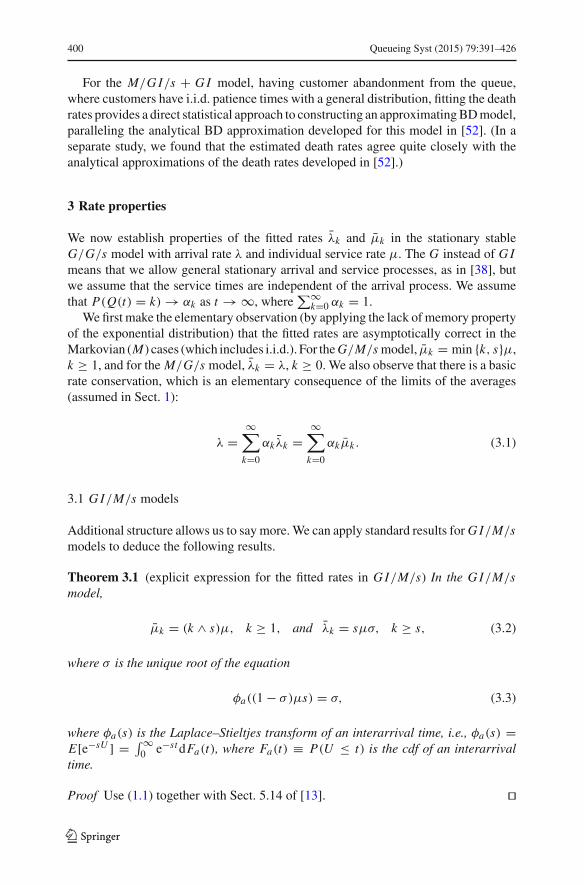
For the M/G I/s + G I model, having customer abandonment from the queue,where customers have i.i.d. patience times with a general distribution, fitting the deathrates provides a direct statistical approach to constructing an approximating BD model,paralleling the analytical BD approximation developed for this model in [52]. (In aseparate study, we found that the estimated death rates agree quite closely with theanalytical approximations of the death rates developed in [52].)

3 Rate properties

We now establish properties of the fitted rates λk and μk in the stationary stableG/G/s model with arrival rate λ and individual service rate μ. The G instead of G Imeans that we allow general stationary arrival and service processes, as in [38], butwe assume that the service times are independent of the arrival process. We assumethat P(Q(t) = k) → αk as t → ∞, where

∑∞k=0 αk = 1.

We first make the elementary observation (by applying the lack of memory propertyof the exponential distribution) that the fitted rates are asymptotically correct in theMarkovian (M) cases (which includes i.i.d.). For the G/M/s model, μk = min {k, s}μ,k ≥ 1, and for the M/G/s model, λk = λ, k ≥ 0. We also observe that there is a basicrate conservation, which is an elementary consequence of the limits of the averages(assumed in Sect. 1):

λ =∞∑

k=0

αk λk =∞∑

k=0

αkμk . (3.1)

3.1 G I/M/s models

Additional structure allows us to say more. We can apply standard results for G I/M/smodels to deduce the following results.

Theorem 3.1 (explicit expression for the fitted rates in G I/M/s) In the G I/M/smodel,

μk = (k ∧ s)μ, k ≥ 1, and λk = sμσ, k ≥ s, (3.2)

where σ is the unique root of the equation

φa((1 − σ)μs) = σ, (3.3)

where φa(s) is the Laplace–Stieltjes transform of an interarrival time, i.e., φa(s) =E[e−sU ] = ∫ ∞

0 e−st dFa(t), where Fa(t) ≡ P(U ≤ t) is the cdf of an interarrivaltime.

Proof Use (1.1) together with Sect. 5.14 of [13]. ��

123

Queueing Syst (2015) 79:391–426 401

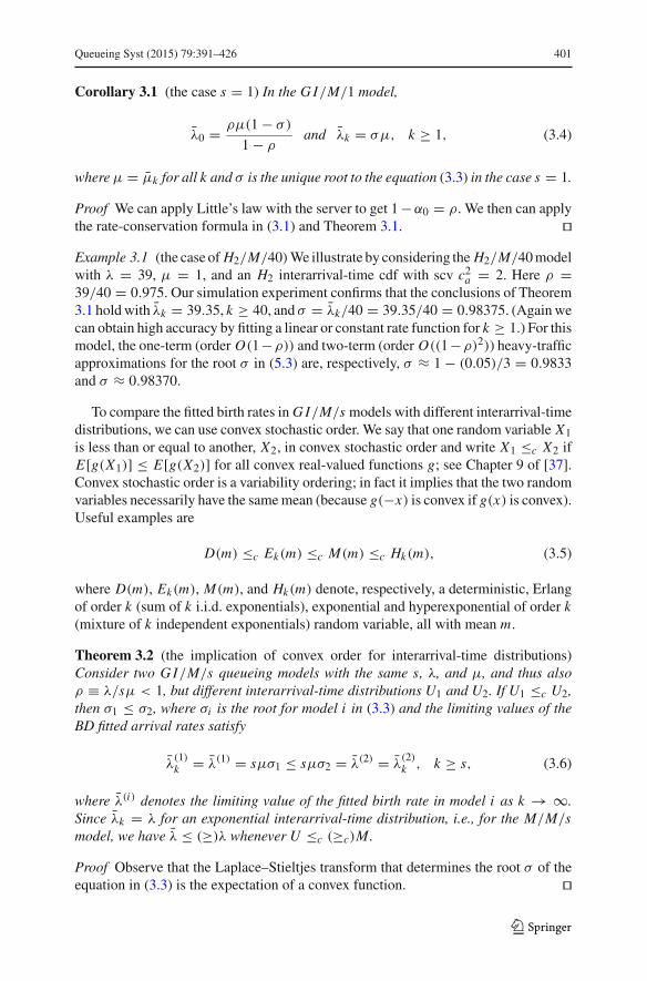
Corollary 3.1 (the case s = 1) In the G I/M/1 model,

λ0 = ρμ(1 − σ)

1 − ρand λk = σμ, k ≥ 1, (3.4)

where μ = μk for all k and σ is the unique root to the equation (3.3) in the case s = 1.

Proof We can apply Little’s law with the server to get 1 −α0 = ρ. We then can applythe rate-conservation formula in (3.1) and Theorem 3.1. ��Example 3.1 (the case of H2/M/40)We illustrate by considering the H2/M/40 modelwith λ = 39, μ = 1, and an H2 interarrival-time cdf with scv c2

a = 2. Here ρ =39/40 = 0.975. Our simulation experiment confirms that the conclusions of Theorem3.1 hold with λk = 39.35, k ≥ 40, and σ = λk/40 = 39.35/40 = 0.98375. (Again wecan obtain high accuracy by fitting a linear or constant rate function for k ≥ 1.) For thismodel, the one-term (order O(1−ρ)) and two-term (order O((1−ρ)2)) heavy-trafficapproximations for the root σ in (5.3) are, respectively, σ ≈ 1 − (0.05)/3 = 0.9833and σ ≈ 0.98370.

To compare the fitted birth rates in G I/M/s models with different interarrival-timedistributions, we can use convex stochastic order. We say that one random variable X1is less than or equal to another, X2, in convex stochastic order and write X1 ≤c X2 ifE[g(X1)] ≤ E[g(X2)] for all convex real-valued functions g; see Chapter 9 of [37].Convex stochastic order is a variability ordering; in fact it implies that the two randomvariables necessarily have the same mean (because g(−x) is convex if g(x) is convex).Useful examples are

D(m) ≤c Ek(m) ≤c M(m) ≤c Hk(m), (3.5)

where D(m), Ek(m), M(m), and Hk(m) denote, respectively, a deterministic, Erlangof order k (sum of k i.i.d. exponentials), exponential and hyperexponential of order k(mixture of k independent exponentials) random variable, all with mean m.

Theorem 3.2 (the implication of convex order for interarrival-time distributions)Consider two G I/M/s queueing models with the same s, λ, and μ, and thus alsoρ ≡ λ/sμ < 1, but different interarrival-time distributions U1 and U2. If U1 ≤c U2,then σ1 ≤ σ2, where σi is the root for model i in (3.3) and the limiting values of theBD fitted arrival rates satisfy

λ(1)k = λ(1) = sμσ1 ≤ sμσ2 = λ(2) = λ

(2)k , k ≥ s, (3.6)

where λ(i) denotes the limiting value of the fitted birth rate in model i as k → ∞.Since λk = λ for an exponential interarrival-time distribution, i.e., for the M/M/smodel, we have λ ≤ (≥)λ whenever U ≤c (≥c)M.

Proof Observe that the Laplace–Stieltjes transform that determines the root σ of theequation in (3.3) is the expectation of a convex function. ��

123

402 Queueing Syst (2015) 79:391–426

More generally, Theorem 3.2 tells us that we expect to have λk ≤ (≥)λ for k ≥ swhenever the arrival process is less (more) variable or bursty than a Poisson process.This ordering helps us interpret fitted birth rates.

3.2 M/G I/s models

For M/G I/s models, the cases s = 1 and s = ∞ are very different in what thefitted rates tell us about the original model, i.e., about the service-time distribution.For s = 1, at least in principle, the fitted death rates tell us everything; for s = ∞, thefitted death rates tell us nothing.

Theorem 3.3 (the M/G I/1 model) For the M/G I/1 model, λk = λ for all k ≥ 0and there is a one-to-one correspondence between the fitted BD death rates μk andthe service distributions with mean 1/μ. Hence, the service-time cdf is exponential ifand only if μk = μ, k ≥ 1.

Proof It is well known that there is a one-to-one correspondence between the steady-state distribution {αk} and the service-time distribution, via the classical Pollaczek-Khintchine generating function, see Sect. 5.8 of [13]. Since there is a one-to-onecorrespondence between the fitted BD rates and the steady-state distribution, the finalconclusion follows. ��

Theorem 3.4 (the M/G I/∞ model) For the M/G I/∞ model, the fitted BD ratessatisfy λk = λ and μk = kμ for all k ≥ 0, just as in the M/M/∞ model.

Proof By the well-known insensitivity property, the steady-state distribution of theM/G I/∞ model is Poisson with mean λ/μ for all service-time distributions withmean 1/μ. Hence, the fitted BD rates are the same as for the M/M/∞ model. ��

3.3 Tail-probability asymptotics: limits as k → ∞

In many G/G/s queueing models, the steady-state distribution of Q(t) has an asymp-totically geometric tail, i.e.,

αk ∼ βσ k as k → ∞, (3.7)

i.e., αk/βσ k → 1 as k → ∞. Hence, for k not too small, the approximation αk ≈ βσ k

is effective and useful; see [2,11] and references therein. However, it is important tonote that (3.7) does not cover all possibilities. For example, with heavy-tail service-time cdf’s we can have

αk ∼ Ak−p as k → ∞ (3.8)

for positive constants A and p.

123

Queueing Syst (2015) 79:391–426 403

Fig. 4 Estimated steady-state probabilities αk (left) and their logarithms loge αk (right) for seven G I/G I/1models with ρ = λ = 0.8 and μ = 1

Theorem 3.5 (limits for the fitted rate ratios) If the steady-state distribution satisfies(3.7), then the limiting fitted BD rate ratios satisfy

ρk ≡ λk

μk+1→ σ as k → ∞. (3.9)

If the arrival process is Poisson, then μk → λ/σ as k → ∞. If instead the steady-statedistribution satisfies (3.8), then the limiting fitted BD rate ratios satisfy

(k + 1) log ρk → −p as k → ∞. (3.10)

Proof For (3.9), use the local balance equation (1.1) with (3.7). For (3.10), use (1.1)with (3.8) to get ρk = p log (1 − [1/(1 + k)]) and then log (1 + ε)/ε → 1 as ε ↓ 0.

��We first illustrate the main case in (3.7) in Fig. 4 by showing the estimated steady-

state probability mass function (left) and its logarithm (right) for the seven G I/G I/1models with λ = ρ = 0.8 and μ = 1 in Fig. 1. The near-linear plots on the rightillustrate the relation (3.7) which is known to hold for all these models. We will exploitthis geometric-tail structure extensively in our conventional heavy-traffic analysis inSect. 5.

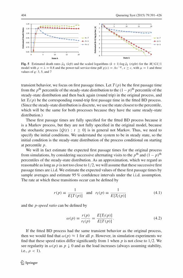
We also illustrate the power-tail case by considering the M/G I/1 queue with aservice-time pdf g(x) = Bx−q , x ≥ c, for B = cq−1/(q − 1) and c chosen so thatit has mean 1/μ = 1. In the case q = 3, this power-tail pdf has an infinite variance.We show the fitted death rates and the estimated values of (k + 1) log ρk in Fig. 5 forthree cases: q = 3, 5, and 7. Figure 5 shows that the estimated death rate is decayingand that (3.8) indeed evidently holds with p = q − 1 = 2 for the case q = 3, butthat (3.7) holds for q = 5 and q = 7. In particular, we see that a power-tail service-time distribution affects the steady-state queue-length distribution differently from thesteady-state waiting time, which always has a power tail in these cases; see [1,12,30]and citations to these papers. We intend to discuss this phenomenon in a future paper.

4 Transient behavior: the speed ratio

We wish to understand how the transient behavior of the fitted BD process differsfrom the transient behavior of the original model. To approximately characterize the

123

404 Queueing Syst (2015) 79:391–426

q

q

q

q

q

q

Fig. 5 Estimated death rates μk (left) and the scaled logarithms (k + 1) log ρk (right) for the M/G I/1model with ρ = λ = 0.8 and the power-tail service-time pdf g(x) = Ax−q , x ≥ c, with μ = 1 and threevalues of q: 3, 5, and 7

transient behavior, we focus on first passage times. Let T (p) be the first passage timefrom the pth percentile of the steady-state distribution to the (1− p)th percentile of thesteady-state distribution and then back again (round trip) in the original process, andlet Tf(p) be the corresponding round-trip first passage time in the fitted BD process.(Since the steady-state distribution is discrete, we use the state closest to the percentile,which will be the same for both processes because they have the same steady-statedistribution.)

These first passage times are fully specified for the fitted BD process because itis a Markov process, but they are not fully specified in the original model, becausethe stochastic process {Q(t) : t ≥ 0} is in general not Markov. Thus, we need tospecify the initial conditions. We understand the system to be in steady state, so theinitial condition is the steady-state distribution of the process conditional on startingat percentile p.

We will in fact estimate the expected first passage times for the original processfrom simulations, by considering successive alternating visits to the pth and (1 − p)th

percentiles of the steady-state distribution. As an approximation, which we regard asreasonable as long as p is not too close to 1/2, we will assume that these successive firstpassage times are i.i.d. We estimate the expected values of these first passage times bysample averages and estimate 95 % confidence intervals under the i.i.d. assumption.The rate at which these transitions occur can be defined by

r(p) ≡ 1

E[T (p)] and rf(p) ≡ 1

E[Tf(p)] (4.1)

and the p-speed ratio can be defined by

ω(p) ≡ r(p)

rf(p)= E[Tf(p)]

E[T (p)] . (4.2)

If the fitted BD process had the same transient behavior as the original process,then we would find that ω(p) ≈ 1 for all p. However, in simulation experiments wefind that these speed ratios differ significantly from 1 when p is not close to 1/2. Wesee regularity in ω(p) as p ↓ 0 and as the load increases (always assuming stability,i.e., ρ < 1).

123

Queueing Syst (2015) 79:391–426 405

4.1 Examples in the conventional heavy-traffic regime

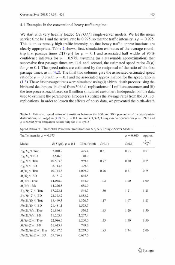
We start with very heavily loaded G I/G I/1 single-server models. We let the meanservice time be 1 and the arrival rate be 0.975, so that the traffic intensity is ρ = 0.975.This is an extremely high traffic intensity, so that heavy-traffic approximations areclearly appropriate. Table 2 shows, first, simulation estimates of the average round-trip first passage times E[T (p)] for p = 0.1 and associated half widths of 95 %confidence intervals for ρ = 0.975, assuming (as a reasonable approximation) thatsuccessive first passage times are i.i.d. and, second, the estimated speed ratios ω(p)

for p = 0.1. The speed ratios are estimated by the reciprocal of the ratio of the firstpassage times, as in (4.2). The final two columns give the associated estimated speedratio for ρ = 0.8 with p = 0.1 and the associated approximation for the speed ratio in(1.3). These first passage times were simulated using (i) a birth–death process using thebirth and death rates obtained from 30 i.i.d. replications of 1 million customers and (ii)the true process, each based on 8 million simulated customers (independent of the dataused to estimate the parameters). Process (i) utilizes the average rates from the 30 i.i.d.replications. In order to lessen the effects of noisy data, we prevented the birth–death

Table 2 Estimated speed ratios of transitions between the 10th and 90th percentile of the steady-statedistributions, i.e., ω(p) in (4.2) for p = 0.1, in nine G I/G I/1 single-server queues for ρ = 0.975 andρ = 0.800, with estimation details only for ρ = 0.975

Speed Ratios of 10th-to-90th Percentile Transitions for G I/G I/1 Single-Server Models

Traffic intensity ρ = 0.975 ρ = 0.800 Approx.

Model E[T (p)], p = 0.1 CI halfwidth ω(0.1) ω(0.1)c2a+c2

s2

E2/E2/1 True 7,010.2 425.4 0.51 0.63 0.5

E2/E2/1 BD 3,546.3 140.9

E2/M/1 True 10,503.3 969.4 0.77 0.80 0.75

E2/M/1 BD 8,113.6 399.3

M/E2/1 True 10,744.8 1,099.2 0.76 0.81 0.75

M/E2/1 BD 8,181.2 645.5

M/M/1 True 14,048.0 544.9 1.02 1.00 1.00

M/M/1 BD 14,276.8 658.9

E2/H2(2)/1 True 17,223.1 544.7 1.30 1.21 1.25

E2/H2(2)/1 BD 22,373.2 1,883.2

H2(2)/E2/1 True 18,449.3 1,320.7 1.17 1.07 1.25

H2(2)/E2/1 BD 21,481.1 1,573.7

H2(2)/M/1 True 21,846.4 550.3 1.43 1.29 1.50

H2(2)/M/1 BD 31,203.4 2,267.4

M/H2(2)/1 True 22,086.6 1,200.0 1.43 1.40 1.50

M/H2(2)/1 BD 31,613.4 749.6

H2(2)/H2(2)/1 True 30,197.6 2,279.0 1.85 1.74 2.00

H2(2)/H2(2)/1 BD 55,786.8 6,677.6

123

406 Queueing Syst (2015) 79:391–426

process from going above the 99.5 percentile. The process is initialized in steady stateby choosing the initial state from the estimated steady-state distribution. The processthen ran for 16 million transitions. In process (i) and process (ii), the system observes1 million and 8 million customers, respectively. The simulation concluded when allcustomers had been served.

Table 2 shows that approximation (1.2) with (1.3) is well justified for single-serverqueues. The estimated speed ratios should be compared to the reference case of 1.00for the M/M/1 model, where the queue-length process is actually a BD process,and the proposed approximation in (1.3) is exactly 1. In all cases, we see that theestimated speed ratio ω(0.1) differs from 1 in the right direction. In all cases exceptone (the E2/H2(2)/1 model for ρ = 0.975), the approximation in (1.3) slightlyoverestimates the difference from 1; i.e., (c2

a + c2s )/2 overestimates (underestimates)

ω when (c2a + c2

s )/2 > 1 (< 1).Of course, it is well known that extremely long simulation runs are required to obtain

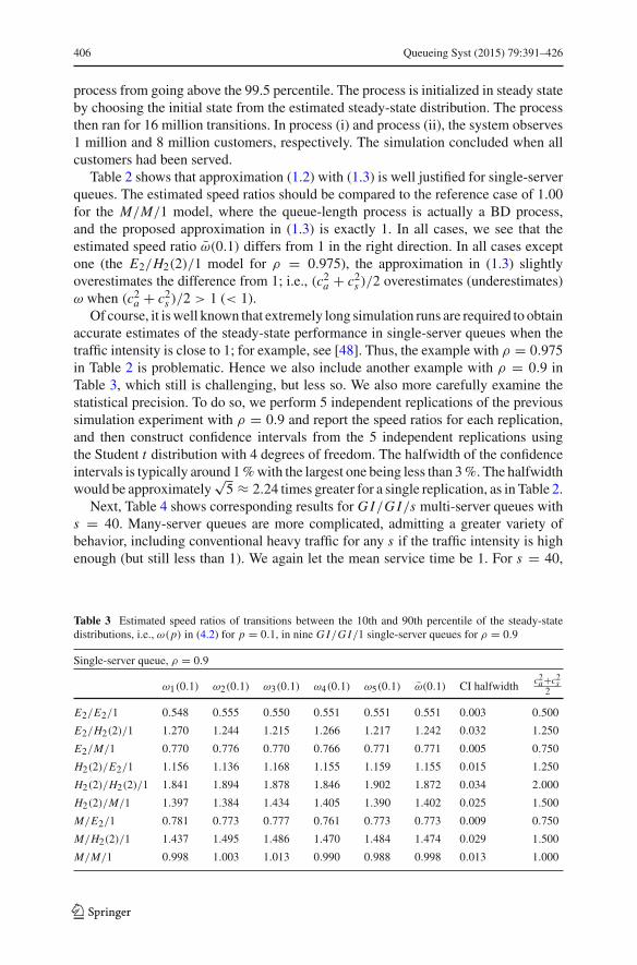
accurate estimates of the steady-state performance in single-server queues when thetraffic intensity is close to 1; for example, see [48]. Thus, the example with ρ = 0.975in Table 2 is problematic. Hence we also include another example with ρ = 0.9 inTable 3, which still is challenging, but less so. We also more carefully examine thestatistical precision. To do so, we perform 5 independent replications of the previoussimulation experiment with ρ = 0.9 and report the speed ratios for each replication,and then construct confidence intervals from the 5 independent replications usingthe Student t distribution with 4 degrees of freedom. The halfwidth of the confidenceintervals is typically around 1 % with the largest one being less than 3 %. The halfwidthwould be approximately

√5 ≈ 2.24 times greater for a single replication, as in Table 2.

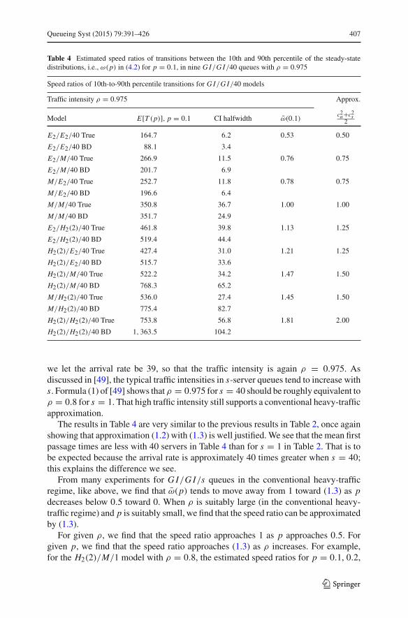
Next, Table 4 shows corresponding results for G I/G I/s multi-server queues withs = 40. Many-server queues are more complicated, admitting a greater variety ofbehavior, including conventional heavy traffic for any s if the traffic intensity is highenough (but still less than 1). We again let the mean service time be 1. For s = 40,

Table 3 Estimated speed ratios of transitions between the 10th and 90th percentile of the steady-statedistributions, i.e., ω(p) in (4.2) for p = 0.1, in nine G I/G I/1 single-server queues for ρ = 0.9

Single-server queue, ρ = 0.9

ω1(0.1) ω2(0.1) ω3(0.1) ω4(0.1) ω5(0.1) ω(0.1) CI halfwidthc2a+c2

s2

E2/E2/1 0.548 0.555 0.550 0.551 0.551 0.551 0.003 0.500

E2/H2(2)/1 1.270 1.244 1.215 1.266 1.217 1.242 0.032 1.250

E2/M/1 0.770 0.776 0.770 0.766 0.771 0.771 0.005 0.750

H2(2)/E2/1 1.156 1.136 1.168 1.155 1.159 1.155 0.015 1.250

H2(2)/H2(2)/1 1.841 1.894 1.878 1.846 1.902 1.872 0.034 2.000

H2(2)/M/1 1.397 1.384 1.434 1.405 1.390 1.402 0.025 1.500

M/E2/1 0.781 0.773 0.777 0.761 0.773 0.773 0.009 0.750

M/H2(2)/1 1.437 1.495 1.486 1.470 1.484 1.474 0.029 1.500

M/M/1 0.998 1.003 1.013 0.990 0.988 0.998 0.013 1.000

123

Queueing Syst (2015) 79:391–426 407

Table 4 Estimated speed ratios of transitions between the 10th and 90th percentile of the steady-statedistributions, i.e., ω(p) in (4.2) for p = 0.1, in nine G I/G I/40 queues with ρ = 0.975

Speed ratios of 10th-to-90th percentile transitions for G I/G I/40 models

Traffic intensity ρ = 0.975 Approx.

Model E[T (p)], p = 0.1 CI halfwidth ω(0.1)c2a+c2

s2

E2/E2/40 True 164.7 6.2 0.53 0.50

E2/E2/40 BD 88.1 3.4

E2/M/40 True 266.9 11.5 0.76 0.75

E2/M/40 BD 201.7 6.9

M/E2/40 True 252.7 11.8 0.78 0.75

M/E2/40 BD 196.6 6.4

M/M/40 True 350.8 36.7 1.00 1.00

M/M/40 BD 351.7 24.9

E2/H2(2)/40 True 461.8 39.8 1.13 1.25

E2/H2(2)/40 BD 519.4 44.4

H2(2)/E2/40 True 427.4 31.0 1.21 1.25

H2(2)/E2/40 BD 515.7 33.6

H2(2)/M/40 True 522.2 34.2 1.47 1.50

H2(2)/M/40 BD 768.3 65.2

M/H2(2)/40 True 536.0 27.4 1.45 1.50

M/H2(2)/40 BD 775.4 82.7

H2(2)/H2(2)/40 True 753.8 56.8 1.81 2.00

H2(2)/H2(2)/40 BD 1, 363.5 104.2

we let the arrival rate be 39, so that the traffic intensity is again ρ = 0.975. Asdiscussed in [49], the typical traffic intensities in s-server queues tend to increase withs. Formula (1) of [49] shows that ρ = 0.975 for s = 40 should be roughly equivalent toρ = 0.8 for s = 1. That high traffic intensity still supports a conventional heavy-trafficapproximation.

The results in Table 4 are very similar to the previous results in Table 2, once againshowing that approximation (1.2) with (1.3) is well justified. We see that the mean firstpassage times are less with 40 servers in Table 4 than for s = 1 in Table 2. That is tobe expected because the arrival rate is approximately 40 times greater when s = 40;this explains the difference we see.

From many experiments for G I/G I/s queues in the conventional heavy-trafficregime, like above, we find that ω(p) tends to move away from 1 toward (1.3) as pdecreases below 0.5 toward 0. When ρ is suitably large (in the conventional heavy-traffic regime) and p is suitably small, we find that the speed ratio can be approximatedby (1.3).

For given ρ, we find that the speed ratio approaches 1 as p approaches 0.5. Forgiven p, we find that the speed ratio approaches (1.3) as ρ increases. For example,for the H2(2)/M/1 model with ρ = 0.8, the estimated speed ratios for p = 0.1, 0.2,

123

408 Queueing Syst (2015) 79:391–426

0.35, and 0.45 were, respectively, 1.29, 1.25, 1.16, and 1.01. On the other hand, forρ = 0.975 all these estimated speed ratios fell in the interval [1.40, 1.50]. Similarly,for the M/E2/1 model with ρ = 0.8, the estimated speed ratios for p = 0.1, 0.2,0.35, and 0.45 were, respectively, 0.81, 0.84, 0.92, and 1.00. On the other hand, forρ = 0.975 all these estimated speed ratios fell in the interval [0.75, 0.78].

As should be anticipated, given this systematic behavior as ρ increases, we find thatinsight can be gained from conventional heavy-traffic theory, which indicates that, ifρ is sufficiently high, then the stochastic process {Q(t) : t ≥ 0} in the G/G/s modelcan be approximated by reflected Brownian motion (a Markov process); we discusssupporting heavy-traffic theory in Sect. 5.

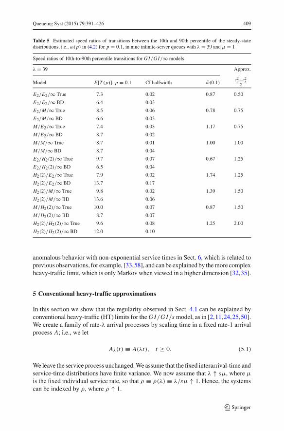
4.2 Examples in the many-server heavy-traffic regime

To show the importance of the heavy-traffic regime, we illustrate with infinite-serverqueues having the same arrival rate λ = 39 as in Table 4. Given that the mean ser-vice time is fixed at 1/μ = 1, the arrival rate of λ = 39 is already quite large, sowe shift from the conventional heavy-traffic regime to the many-server heavy-trafficregime as we increase the number of servers. The many-server heavy-traffic regime ischaracterized by λ → ∞ and s → ∞ with fixed μ such that

√s(1 − ρ) → β < ∞;

see [21,31,35,51]. The essential character is seen by considering s = ∞. (It can beimportant to consider subcases, but we do not do so here.)

Table 5 shows the results of the simulation experiment in the infinite-server cases.First, we see that the mean first passage times between the percentiles are less inTable 5 than in Table 4, even though the arrival rate is λ = 39 in both cases. That canbe explained because the steady-state distribution is more concentrated (less variable)with infinitely many servers. The extra servers prevent excursions to very large values.

As before, the estimated speed ratios ω(p) differ from 1 as p moves away from 0.5toward 0. We find that the speed ratios in the infinite-server case do match the formulasabove for the G I/M/∞ models, but not for the other queues with non-exponentialservice distributions. For example, for the H2(2)/M/s model with λ = 39 and μ = 1,we have ω(0.1) = 1.49 when s = 40 and 1.39 when s = ∞. In striking contrast, for theM/H2(2)/s model with λ = 39 and μ = 1, we have ω(0.1) = 1.42 when s = 40 and0.87 when s = ∞. In both cases, approximation (1.3) yields ω = (c2

a + c2s )/2 = 1.5.

For the M/H2(2)/∞ case, the estimated speed ratio is not close to 1.5, but less than1, and thus in the wrong direction away from 1.

We do see impressive regularity in Table 5 beyond the G I/M/∞ model for whichapproximation (1.3) remains good. More generally, we observe that the estimatedspeed ratios ω(0.1) are consistently increasing in c2

a but decreasing in c2s .

For infinite-server queues and associated many-server queues in the many-serverheavy-traffic regime, we again suggest the approximation in (1.2), but with (1.3) onlyin the case of G/M/∞ and G/M/s queues. Insight into the good performance of (1.2)with (1.3) for G/M/∞ and G/M/s queues can be gained from many-server heavy-traffic limits, indicating that the stochastic process {Q(t) : t ≥ 0} can be approximatedby ρ + √

ρX (t), where ρ ≡ λ/μ and X (t) is an Ornstein-Uhlenbeck (OU) diffusionprocess in the infinite-server case; see [45]; we discuss in Sect. 6. We also explain the

123

Queueing Syst (2015) 79:391–426 409

Table 5 Estimated speed ratios of transitions between the 10th and 90th percentile of the steady-statedistributions, i.e., ω(p) in (4.2) for p = 0.1, in nine infinite-server queues with λ = 39 and μ = 1

Speed ratios of 10th-to-90th percentile transitions for G I/G I/∞ models

λ = 39 Approx.

Model E[T (p)], p = 0.1 CI halfwidth ω(0.1)c2a+c2

s2

E2/E2/∞ True 7.3 0.02 0.87 0.50

E2/E2/∞ BD 6.4 0.03

E2/M/∞ True 8.5 0.06 0.78 0.75

E2/M/∞ BD 6.6 0.03

M/E2/∞ True 7.4 0.03 1.17 0.75

M/E2/∞ BD 8.7 0.02

M/M/∞ True 8.7 0.01 1.00 1.00

M/M/∞ BD 8.7 0.04

E2/H2(2)/∞ True 9.7 0.07 0.67 1.25

E2/H2(2)/∞ BD 6.5 0.04

H2(2)/E2/∞ True 7.9 0.02 1.74 1.25

H2(2)/E2/∞ BD 13.7 0.17

H2(2)/M/∞ True 9.8 0.02 1.39 1.50

H2(2)/M/∞ BD 13.6 0.06

M/H2(2)/∞ True 10.0 0.07 0.87 1.50

M/H2(2)/∞ BD 8.7 0.07

H2(2)/H2(2)/∞ True 9.6 0.08 1.25 2.00

H2(2)/H2(2)/∞ BD 12.0 0.10

anomalous behavior with non-exponential service times in Sect. 6, which is related toprevious observations, for example, [33,58], and can be explained by the more complexheavy-traffic limit, which is only Markov when viewed in a higher dimension [32,35].

5 Conventional heavy-traffic approximations

In this section we show that the regularity observed in Sect. 4.1 can be explained byconventional heavy-traffic (HT) limits for the G I/G I/s model, as in [2,11,24,25,50].We create a family of rate-λ arrival processes by scaling time in a fixed rate-1 arrivalprocess A; i.e., we let

Aλ(t) ≡ A(λt), t ≥ 0. (5.1)

We leave the service process unchanged. We assume that the fixed interarrival-time andservice-time distributions have finite variance. We now assume that λ ↑ sμ, where μ

is the fixed individual service rate, so that ρ ≡ ρ(λ) ≡ λ/sμ ↑ 1. Hence, the systemscan be indexed by ρ, where ρ ↑ 1.

123

410 Queueing Syst (2015) 79:391–426

As indicated in Sect. 2.1, it is important to note that the key parameters λ, μ, ρ,and ω estimated in Table 1, as well as the fitted birth rates λk and the fitted death ratesμk , depend on ρ. (This can be seen by comparing the cases ρ = 0.8 and ρ = 0.9 inTables 1 and 6.)

We now need to understand how ρ(ρ) ≡ λ(ρ)/μ(ρ) changes with ρ. For thatpurpose, we assume that the geometric tail in (3.7) is valid for each ρ. We also assumethat the estimated rates have limits as k → ∞, i.e.,

λk(ρ) → λ(ρ) and μk(ρ) → μ(ρ) as k → ∞ for each ρ. (5.2)

The value of the asymptotic relation (3.7) is enhanced by heavy-traffic expansionsgiven in [2,11], which we assume are valid here as well. We state the one for theG I/G I/s model from [2]. Let uk and vk be the kth moments of the mean-1 randomvariables U/E[U ] = λU and V/E[V ] = μV , where U is a generic interarrival timeand V is a generic service time. Under quite general regularity conditions, as 1−ρ ↓ 0,

σ(ρ) = 1 − 2(1 − ρ)

c2a + c2

s+

(8(ds − da)

(c2a + c2

s )3 − 2(c2

a − 1)

(c2a + c2

s )2

)

(1 − ρ)2 + O((1 − ρ)3),

(5.3)

where c2a ≡ u2 − u2

1 = u2 − 1 and c2s ≡ v2 − v2

1 = v2 − 1 are the squared coefficientsof variation (scv’s, variances divided by the square of the mean) of the interarrivaltime λU and service time μV , respectively, while da and ds are parameters based onthe first three moments of λU and μV , namely,

da ≡ u3 − 3c2a(c2

a + 1) − 1

6and ds ≡ v3 − 3c2

s (c2s + 1) − 1

6. (5.4)

We thus can combine previous results to obtain the asymptotic behavior of ρ(ρ) ≡λ(ρ)/μ(ρ), which we regard as the traffic intensity of the fitted BD model.

Theorem 5.1 (HT limit for the fitted traffic intensity of the fitted BD model) If afamily of G/G/s models is created using (5.1), where (5.2), (3.7), and (5.3) are valid,then

ρ(ρ) ≡ λ(ρ)

μ(ρ)= σ(ρ) for each ρ, (5.5)

where σ(ρ) is determined by (3.7) and

ω(ρ) ≡ 1 − ρ

1 − ρ(ρ)= ω + O(1 − ρ) as ρ ↑ 1. (5.6)

for ω ≡ (c2a + c2

s )/2 in (1.3).

Proof Combine (1.1) with (3.7) to get (5.5). Then apply (5.3) to get (5.6). ��

123

Queueing Syst (2015) 79:391–426 411

We anticipate that, under regularity conditions, the entire fitted BD process shouldhave the same HT limit as the queue-length process in an M/M/1 queue with constantarrival rate λ(ρ), constant service rate μ(ρ), and traffic intensity ρ ≡ ρ(ρ), when welet ρ(ρ) ↑ 1 as ρ ↑ 1 as in (5.6). In addition to (5.2), we now also need an additionalcondition, which we formulate in the following conjecture. It is a generalization of(2.1), which holds for all G I/M/s models by Theorem 3.1.

Conjecture 5.1 (conventional HT limit for fitted birth and death rates) If the con-ditions of Theorem 5.1 hold, then there exist finite constants λ(1−), μ(1−) and k0,depending on the arrival and service processes, such that λ(1−) > μ(1−),

supk:k≥k0

{|λρ,k − [μs − λ(1−)(1 − ρ)]|} = o(1 − ρ) as ρ ↑ 1, and

supk:k≥k0

{|μρ,k − [μs − μ(1−)(1 − ρ)]|} = o(1 − ρ) as ρ ↑ 1. (5.7)

The leading term sμ of both functions λρ,k and μρ,k in (5.7) is the overall maximumpossible service rate. The notation in (5.7) suggests that the functions λ(ρ) and μ(ρ)

in (5.2) are differentiable functions of ρ for 0 < ρ < 1, with the derivatives havingfinite left limits λ(1−) and μ(1−) as ρ ↑ 1, which we also conjecture is the case, butthat structure is not required.

We now establish a heavy-traffic limit under the conditions of Conjecture 5.1.Let D be the standard function space of right-continuous functions on [0,∞) withleft limits everywhere and with the Skorohod topology and let ⇒ denote conver-gence in distribution in the function space D, as in [50]. Let R ≡ {R(t; a, b) :t ≥ 0} be a reflected Brownian motion (R B M) with drift coefficient a and diffusioncoefficient b.

Theorem 5.2 (HT limit for fitted BD process) If the conditions and the conclusion ofConjecture 5.1 hold, then

{(1 − ρ)Q f,ρ((1 − ρ)−2t) : t ≥ 0}⇒ {R(t;−μs/ω, 2μs) : t ≥ 0} in D as ρ ↑ 1. (5.8)

Proof We do the proof in three steps. First, we do the proof for the case in which

λρ,k = μs − λ(1−)(1 − ρ) and μρ,k = μs − μ(1−)(1 − ρ) for all k

(5.9)

and then in the remaining two steps we show that the limit has to be the same asunder condition (5.9). The condition (5.9) corresponds to a family of M/M/1 modelswith the specified arrival and service rates, for which established heavy-traffic limitsin [24,25,50] imply convergence to RBM with drift coefficient −(λ(1−) − μ(1−))

and variance coefficient 2μs. However, Theorem 5.1 and simple algebra imply thatλ(1−) − μ(1−) = μs/ω. Hence, we get the limit in (5.8).

123

412 Queueing Syst (2015) 79:391–426

For the second step, we assume that the relation in (5.7) holds for all k, not justfor k ≥ k0. Under this strengthened version of condition (5.7), we can bound thefitted birth rates and death rates above and below arbitrarily closely, in the sense that,for any ε > 0, we can find ρ(ε), λL(1−), λU (1−), μL(1−), and μU (1−) such that0 ≤ ρ(ε) < 1, λU (1−) − λL(1−) < ε, μU (1−) − μL(1−) < ε,

sμ − λU (1−)(1 − ρ) ≤ λρ,k ≤ sμ − λL(1−)(1 − ρ) and

sμ − μU (1−)(1 − ρ) ≤ μρ,k ≤ sμ − μL(1−)(1 − ρ)

for all k ≥ 1 and ρ > ρ(ε). (5.10)

We can then construct upper and lower bounds for the family of BD processesQ f,ρ(t) in sample path stochastic order; i.e., we can construct three processes Q f,ρ(t),Q f,ρ,L(t), and Q f,ρ,U (t) such that

Q f,ρ,L(t) ≤ Q f,ρ(t) ≤ Q f,ρ,U (t) for all t w. p. 1,

where all three processes have the proper distributions as BD processes, with {Q f,ρ(t) :t ≥ 0} distributed the same as {Q f,ρ(t) : t ≥ 0}. This is done by generating all transi-tions from common Poisson processes. We let higher processes have births wheneverlower ones do; we let lower processes have deaths whenever higher processes do;in this way the sample paths stay ordered. By choosing ε suitably small, the threeprocesses can be made to have identical sample paths over any finite interval [0, t]with probability arbitrarily close to 1. As in [43], the upper-bound BD process hasthe upper-bound birth rates sμ − λL(1−)(1 − ρ) and the lower-bound death ratessμ − μU (1−)(1 − ρ), while the lower-bound BD process has the lower-bound birthrates sμ − λU (1−)(1 − ρ) and the upper-bound death rates sμ − μL(1−)(1 − ρ).These bounding BD processes satisfy the assumptions of the first part, but with dif-ferent parameters, and so have heavy-traffic limits. By letting ε ↓ 0, we can sandwichthe process Q f,ρ(t) between these bounding processes and obtain the limit in the firststep.

For the third step, we observe that the limit under condition (5.7) must be thesame as in the first two steps because the processes Q(t) and Qf(t) spend asymp-totically negligible time in the states with k ≤ k0. The space scaling thus makesthe difference asymptotically negligible; i.e., we can apply the “convergence-togethertheorem,” Theorem 11.4.7 of [50]. ��

Recall from [25] that the heavy-traffic limit of the scaled queue-length process inthe G/G/s model is

{(1−ρ)Q((1−ρ)−2t) : t ≥0} ⇒ {ωR(t;−sμ, 2sμω) : t ≥ 0} in D, (5.11)

which differs from (5.8) by having the variability parameter ω as part of the diffusioncoefficient instead of part of the drift.

We now show that these approximating RBM’s can be related as in (1.2). To see thisdirectly, it is convenient to rescale these limiting RBM’s to canonical RBM’s (withdrift coefficient −1 and diffusion coefficient 1), for example, using (25) of [48].

123

Queueing Syst (2015) 79:391–426 413

Corollary 5.1 (simple time transformation) The two approximating RBM’s in (5.8)and (5.11) correspond to the following scaled canonical RBM’s:

{R(t;−μs/ω, 2μs) : t ≥ 0} d= {2ωR(μst/(2ω2);−1, 1) : t ≥ 0} and

{ωR(t;−sμ, 2sμω) : t ≥ 0} d= {2ωR(μst/(2ω);−1, 1)) : t ≥ 0}. (5.12)

The representation (5.12) implies that the two RBM’s have a common exponentialsteady-state distribution with mean ω and that, under the conditions of Theorem 5.2,the simple time transformation in (1.2) is asymptotically correct (in distribution) inthe heavy-traffic limit.

Proof Since R B M(t;−a, b) with a, b > 0 has an exponential steady-state distribu-tion with mean b/2a, the RBM’s in (5.8), (5.11), and (5.12) all have an exponentialsteady-state distribution with mean ω, consistent with the fact the the fitted BD processmust have the same steady-state distribution as the original queue-length process. Forthe transient behavior, we see that the two RBM’s in (5.12) are identical except thatthe RBM limit for the fitted BD process has an extra ω in the denominator of the timescaling. ��

We have numerically studied this effect via the speed ratios. Let Tρ(p) be the firstpassage time from percentile p of the stationary distribution to percentile 1 − p ofthe stationary distribution and then back in the original model, and let T f,ρ(p) be thecorresponding round-trip first passage time in the fitted BD process. We can apply thelimits in (5.8) and (5.11) with (5.12) to obtain corresponding limits for the first passagetimes and then the speed ratios. The results above immediately imply the followingcorollary.

Corollary 5.2 (HT limit for the speed ratios) If the limits in (5.8) and (5.11) hold,then

T f,ρ(p)

Tρ(p)⇒ c2

a + c2s

2≡ ω as ρ ↑ 1 (5.13)

and, assuming associated uniform integrability,

E[T f,ρ(p)]E[Tρ(p)] → c2

a + c2s

2≡ ω as ρ ↑ 1 (5.14)

for all p with 0 < p < 1/2 as ρ ↑ 1.

Proof We can establish limits for the first passage times of each process separatelyusing the standard continuous mapping theorem argument, provided that the statespace is scaled consistently with the HT scaling; see Sect. 5.7.5 of [50]. We achievethat scaling of the state space by looking at the first passage times between percentilesof the stationary distribution, which is the same for both processes. ��

We conclude this section by giving two numerical examples.

123

414 Queueing Syst (2015) 79:391–426

Example 5.1 (the case of M/H2/1) We now illustrate by considering the M/H2/1model with λ = 0.8, μ = 1, and an H2 service-time cdf Fs(x) with scv c2

s = 2 andbalanced means. For this model, the steady-state distribution is given by the Pollaczek-Khintchine generating function; see Sect. 5.8 of [13]. The mean has the well-knownexplicit form E[Q(∞)] = ρ + (ρ2(c2

s + 1)/2(1 − ρ)). For M/M/1 the mean is 4.8;for M/H2/1 with c2

s = 2, the mean is 5.6. For M/H2/1, αk decays somewhat moreslowly.

We simulated this M/H2/1 model. The estimated birth rates are essentially exact,fitting a constant function well, while the estimated death rates were μ1 = 1.181, μ2 =1.072, μ3 = 0.999, μ4 = 0.965 and μk approaching the constant value of about 0.925.Thus, the estimated value of σ in Theorem 3.5 is λk/μk+1 ≈ 0.8/0.925 ≈ 0.865,which is consistent with the first term in the heavy-traffic approximation, 0.867.

Example 5.2 (the case of M/H2/40) We also illustrate an example with s > 1 byconsidering the M/H2/40 model with λ = 39, μ = 1, and the same H2 service-time cdf as in Example 5.1. Here ρ = 39/40 = 0.975. we simulated this M/H2/40model, as described in the next section. Our simulation experiment confirms that thefitted birth rates are exact. Over the region most frequently visited, i.e., [20, 100],the death rates μk(∞) were first slightly greater than the corresponding M/M/sdeath rates but then eventually lower, with the crossover point being k = 52. Forexample, μ30(∞) = 30.31 > 30, μ35(∞) = 35.59 > 35, μ40(∞) = 40.318 > 40with a peak at μ42(∞) = 40.758 and then steadily but gradually declining withμ52(∞) ≈ 40.000 and approaching μk(∞) = 39.67 for large k. Thus, the estimatedvalue of σ in Theorem 3.5 is λk(∞)/μk+1(∞) ≈ 39.0/39.67 ≈ 0.9831, which isconsistent with the first term in the heavy-traffic approximation, 0.9833.

6 Heavy-traffic approximations for infinite-server models

We now discuss the results for infinite-server queues in Table 5.

6.1 Heavy-traffic limit for the fitted BD process

We have seen that the fitted birth and death rates in a G I/G I/∞ infinite-server modeltend to have, at least approximately, the structure in equations (2.3) and (2.5). Togain insight, we establish many-server heavy-traffic limits for such BD processes. Let{Qn(t) : t ≥ 0} be the BD stochastic process as a function of n, n ≥ 1, and considerthe scaled stochastic processes defined by

Qn(t) ≡ n−1/2(Qn(t) − n), t ≥ 0, n ≥ 1. (6.1)

Theorem 6.1 (HT limit for BD processes with asymptotically linear birth rate) Con-sider a sequence of fitted BD processes associated with a G I/G I/∞ model indexedby the arrival rate n, satisfying Conjectures 2.1 and 2.2, which includes the special

123

Queueing Syst (2015) 79:391–426 415

case in (2.3) and (2.5). If

Qn(0) ⇒ L in R as n → ∞, (6.2)

where P(L < ∞) =1, then

{Qn(t) : t ≥ 0} ⇒ {OU (t; 1 − b, 2) : t ≥ 0} in D, (6.3)

where OU (0)d= L and {OU (t; 1 − b, 2) : t ≥ 0} is an Ornstein-Uhlenbeck (OU)

diffusion process evolving independently conditional on OU (0), with drift functionμ(x) = −(1 − b)x and diffusion function σ 2(x) = σ 2 = 2, which has a Gaussiansteady-state distribution with mean 0 and variance 1/(1 − b).

Proof We follow the approach used by Iglehart [23] for the M/M/∞ model andapply the limit theorem for BD processes developed by Stone [40]. To apply thattheorem here, it suffices to show that the infinitesimal means and variances of the BDprocesses converge to the drift and diffusion functions of the OU diffusion process.For the infinitesimal mean, let xn be a possible value of Qn(t) such that xn → x asn → ∞. Then

mn(xn) ≡ limh→0

E[(Qn(t + h) − Qn(t))/h|Qn(t) = xn]= lim

h→0E[(Qn(t + h) − Qn(t))/h

√n|Qn(t) = n + √

nxn]

= λn,n+√nxn

− μn+√nxn√

n

= n + b(n + √nxn − n) − (n + √

nxn) + o(√

n)√n

= (b − 1)xn + o(1) → (b − 1)x as n → ∞. (6.4)

For the infinitesimal variance,

σ 2n (xn) ≡ lim

h→0E[(Qn(t + h) − Qn(t))2/h|Qn(t) = xn]

= limh→0

E[(Qn(t + h) − Qn(t))2/hn|Qn(t) = n + √nxn]

= λn,n+√nxn

+ μn+√nxn

n

= n + b(n + √nxn − n) + (n + √

nxn) + o(√

n)

n→ 2 as n → ∞.

(6.5)

It is well known that the steady-state distribution of the OU process is Gaussian withmean 0 and variance σ 2/2|μ|, which here takes the value 1/(1 − b). ��

123

416 Queueing Syst (2015) 79:391–426

Corollary 6.1 (identifying the constant b) To have the same steady-state distributionas the G I/M/∞ model, the drift of the limiting OU process in Theorem 6.1 must beμ(x) = −1/ω, where ω ≡ (c2

a + 1)/2 is the speed ratio.

Proof Theorem 1 of [45] implies that the HT limit for the G I/M/∞ model is also anOU process with mean 0 but variance equal to ω ≡ (c2

a + 1)/2. Since the steady-statedistribution of the fitted BD process coincides with the steady-state distribution of theG I/M/∞ model as the sample size increases, if the birth rates are as in (2.5), thenwe must have

1

1 − b= ω or b − 1 = 1

ω= 2

c2a + 1

. (6.6)

��

Since the speed ratio is defined in terms of the first passage times, we need toexploit associated HT limits for the first passage times. We first need to establish acorresponding limit for the steady-state distributions.

Theorem 6.2 (HT limit for steady-state distributions) Under the conditions of Theo-rem 6.1,

Qn(t) ⇒ Qn(∞) in R as t → ∞, (6.7)

where Qn(∞) is a proper random variable for each n and

Qn(∞) ⇒ OU (∞; 1 − b, 2)d= N (0, 1/(1 − b)) in R as n → ∞. (6.8)

Proof We follow the argument used to prove Theorem 2 of [45]. We first prove that(6.7) holds and show that the sequence {Qn(∞) : n ≥ 1} is tight. We give a detailedderivation under the simplified structure in (2.3) and (2.5). The same conclusions canbe shown to hold under Conjectures 2.1 and 2.2. Toward that end, note that, from (2.5)and (2.3), the stochastic process |Qn(t)−n| is directly a BD process on the nonnegativeintegers for each n with birth rate bn,k ≡ n + bk and death rate dn,k ≡ n + k, where−∞ < b < 1, so that we can directly calculate its steady-state distribution using thefamiliar BD formulas

αn,k ≡ limt→∞ P(Qn(t) = k) = rn,k

∑∞j=0 rn, j

, (6.9)

where rn,0 ≡ 1 and

rn,k = bn,0 × · · · × bn,k−1

dn,1 × · · · × dn,k= n(n + b) × · · · × (n + k − 1)

(n + 1) × · · · × (n + k)(6.10)

123

Queueing Syst (2015) 79:391–426 417

for k ≥ 1. Hence,

loge rn,k =k−1∑

j=0

loge (1 + ( jb/n)) −k∑

j=1

loge (1 + ( j/n)), (6.11)

so that

loge rn, k ∼k−1∑

j=0

( jb/n) −k∑

j=1

( j/n) = b(k − 1)k

2n− k(k + 1)

2nas n → ∞

(6.12)

and

rn,c√

n ∼ e−(1−b)c2/2 for b < 1. (6.13)

From (6.13), we can deduce that |Qn(t)−n| has a proper steady-state limit |Qn(∞)−n|for all n sufficiently large, and that the sequence {n−1/2|Qn(∞) − n| : n ≥ 1} is tightin R. That implies that the sequence {Qn(∞) : n ≥ 1} is tight. By symmetry, we seethat Qn(t)−n has a steady-state distribution for each n, which implies that Qn(t) doesas well. From the tightness of {Qn(∞) : n ≥ 1}, we know that there is a convergentsubsequence. We consider such a convergent subsequence and make those terms theinitial values Qn(0) in (6.2). Those initial values make the scaled BD processes strictlystationary processes for each n. However, we can also invoke Theorem 6.1. That allowsus to identify the limit of the convergent subsequence of {Qn(∞) : n ≥ 1}. Since everyconvergent subsequence must have that same limit, we actually have convergence, i.e.,we have proved (6.8). ��

Again, let Tp be the round-trip first passage time from the pth percentile of thesteady-state distribution to the (1 − p)th percentile and back. Just as for Corollary 5.2in the conventional heavy-traffic regime, the asymptotics for the speed ratio here inthe many-server heavy-traffic regime depend on key differences in the heavy-trafficdiffusion stochastic-process limits for the fitted BD process and the original queue-ing process. We have already observed that both limit processes are OU diffusionprocesses, but the parameters of those OU processes are different. For the fitted BDprocess, the drift and diffusion parameters were −(1 − b) = −2/(1 + c2

a) and 2,respectively. From Theorem 1 of [45], we see that for the original G I/M/∞ queue-length process, both of these parameters are multiplied by ω ≡ (1 + c2

a)/2; the driftand diffusion parameters G I/M/∞ queue-length process are −1 and (1 + c2

a). Thischange makes the asymptotic value of the speed ratio ω, as we now show.

Corollary 6.2 Under the conditions of Theorem (6.1),

Tp(Qn) ⇒ Tp(OU ) in R as n → ∞, (6.14)

123

418 Queueing Syst (2015) 79:391–426

where Qn is the BD process with the fitted rates in (2.5) and (2.3), OU ≡ {OU (t; 1−b, 2) : t ≥ 0} and

E[Tp(OU (·, μ, σ 2)] = E[Tp(OU (·, 1, 2))]1 − b

. (6.15)

As a consequence, the speed ratios in the G/M/∞ model satisfy

ωn → ω ≡ c2a + 1

2as n → ∞.

Proof By Theorem 6.2, the steady-state distributions converge. Hence, the percentilesof the scaled process converge to the percentiles of the limit process. Thus, the limit in(6.14) follows from the continuous mapping theorem, as on p. 447 of [50]. Equation(6.15) follows from [10]; see also (2.3) of [41]. By focusing on the first passagetimes from one percentile to another, we automatically achieve the space and timetransformation in (3.4)–(3.7) of [10]. ��

6.2 Supporting theory for M/G I/∞ models

We now discuss the anomalous behavior observed in Table 5 for the M/G I/∞ models.First, Theorem 3.4 implies for M/G I/∞ models that the birth and death rates coincidewith those in the associated M/M/∞ BD model. In contrast, for the G I/G I/s modelin the conventional heavy-traffic regime, the mean steady-state number in the systemtends to be directly proportional to the speed ratio ω = (c2

a +c2s )/2. Thus, the distance

between the percentiles of the steady-state distribution is radically different for theM/G I/∞ model.

The transient behavior of the M/G I/∞ model with large arrival rate is also morecomplicated than for the other models. For the G I/M/∞ model and for the G I/G I/smodel in the conventional heavy-traffic regime, the heavy-traffic approximations areMarkov processes. In contrast, the transient behavior of the M/G I/∞ model dependsstrongly on the elapsed service times (ages) of the customers in service. Simpleapproximations are less likely to be effective because the heavy-traffic approximatingprocesses are not Markov unless the dimension of the state is increased, as shown in[32,35] and references therein. Our approach based on first passage times does notkeep track of that full expanded state.

Nevertheless, the transient behavior of the M/G I/∞ model can be understoodand approximated, as shown in [17,18], but it leads to a different story. It does notsupport approximation (1.2) with (1.3). Suppose that S denotes a service time withcdf G. First, we have just noted that the percentiles of the stationary distribution areindependent of the service-time distribution beyond its mean. However, as indicatedin Theorem 1 of [18] and Sect. 2 of [17], the transient behavior depends largely onthe service-time cdf G through the stationary-excess cdf associated with G, denotedby Ge. Let Se denote a random variable with cdf Ge. Then

123

Queueing Syst (2015) 79:391–426 419

Ge(t) ≡ P(Se ≤ t) = 1

E[S]∫ t

0P(S > u) du with E[Se] = E[S](1 + c2

s )

2.

(6.16)

Thus, if c2s > 1 as for the H2 cdf, E[Se] > E[S], while if c2

s < 1 as for the E2 cdf,E[Se] < E[S].

Understanding of the transient behavior of these G/G I/∞ infinite-server models isenhanced by recognizing that new arrivals can be treated separately from old content.First, suppose that we consider the evolution of the customers in the system, giventhat we consider the system in steady state under the condition that we start at a highpercentile of the stationary distribution (for example, the 90th percentile). Theorem 1[17] implies that the remaining service times of the customers in service are distributedas i.i.d. random variables distributed according to Se. This implies that if the service-time distribution is H2 with c2

s > 1, then the time for the excess number of customersto depart will tend to be longer than if the service time were exponential. If we startwith n busy servers, then the mean number of these servers still busy with the samecustomers at time t is nGe(t). These results indicate that, from this perspective, thetransient behavior of the M/G I/∞ model with H2 service will be slower than if theservice time were exponential, consistent with our simulation results.

Now consider the new arrivals, starting empty. That is unambiguously defined witha Poisson arrival process. The mean number of busy servers (which coincides with thenumber of customers in the system) increases toward its steady-state limit λE[S]. Asshown in (20) of [18], the expected proportion of this mean achieved by time t turnsout be equal to Ge(t). Since this cdf has mean E[Se] = E[S](c2

s + 1)/2, we see thatthe mean increases more slowly than would be the case if c2

s = 1.This analysis of the M/G I/∞ model does not apply directly to the first passage

times, which tend to depend on the ages of the customers in service. Nevertheless, thisanalysis leads to the conclusion that, roughly, the process Q(t) with H2 service movesmore slowly than the corresponding process with M service by a factor of (c2

s + 1)/2,which is exactly the speed ratio in (1.3). That supports approximation (1.2) but with aspeed ratio equal to the reciprocal of the formula in (1.3), which is roughly consistentwith the simulation results in Table 5.

It remains to consider more general G/G I/∞ models. Given research on thosemodels in [32–34], we anticipate the story will be more complicated.

7 Estimation methods

We now discuss two estimation issues: (i) estimating the speed ratios and (ii) estimatingthe birth and death rates of the fitted model.

7.1 Estimating the speed ratios

We clearly can estimate the mean round-trip first passage times E[T (p)] and E[Tf(p)]in Sect. 4 by the sample averages of successive observed passage times, just as we

123

420 Queueing Syst (2015) 79:391–426

did in the simulation experiments. That leads directly to estimates of the speed ratiosω(p) in (4.2). However, there is an alternative approach via the arrival and servicecounting processes A(t) and S(t) ≡ D(t)/B(t) defined in Sect. 2.1 that allows fordependence among interarrival times and service times. The key is the observation thatthe heavy-traffic limit theorems characterizing the asymptotic speed ratio ω actuallydepend on the arrival process through the FCLT for A(t), and similarly for the serviceprocess S(t) when s < ∞; see [25,32].

To account for the dependence, it is natural to work with indices of dispersion, asin [14,20,39] and Sect. 9.6 of [50]. Given a stationary sequence of interarrival times,the index of dispersion for intervals (IDI) is defined as

Ii (n) ≡ V ar(U1 + · · · + Un)

nE[Un]2 , n ≥ 1, (7.1)

while the associated index of dispersion for counts (IDC) is defined as

Ic(t) ≡ Var(A(t))

E[A(t)] , t ≥ 0, (7.2)

The heavy-traffic limits correspond to the limiting values, i.e.,

c2a = lim

n→∞ Ii (n) = limt→∞ Ic(t). (7.3)

Similar results hold for c2s . Hence, we should want to estimate the IDI for relatively

large n and the IDC for relatively large t .

7.2 Rate estimation methods

In this section we discuss ways to enhance the rate estimation.

7.2.1 Piecewise-linear fits

If we are confident that we have a G I/G I/s model, or if we perform a rate estimationand obtain results as in Sect. 2, we can obtain more reliable estimates for individualrates if we fit piecewise-linear functions. In particular, for the single-server modelswith ρ = 0.8 in Sect. 2.1, we can exploit (2.1) and fit linear or constant functions fork ≥ s. For s-server models with relatively large s, like 40, we can exploit (2.3) and(2.5) and fit functions of that piecewise-linear form. For system data, we presumablydo not want to do this initially, because a major goal may be to detect deviations fromthe G/G/s model, as discussed in Sect. 2.3.

7.2.2 Smoothing: binomial averaging

More generally, more reliable estimates for individual rates can be obtained usingsmoothing techniques. The state-dependent birth and death rates in each state are

123

Queueing Syst (2015) 79:391–426 421

likely to be similar to those in neighboring states. Thus, smoothing can be utilizedto refine the rate estimation and to reduce the amount of data needed to accuratelyestimate the birth and death rates. In our simulation experiments, we used very largesample sizes, but in applications that may not be possible, because the model maychange over different time intervals of each day and over different days; for example,see [27].

In our simulation experiments we investigated various smoothing methods. Weremark that we found binomial averaging to be an effective smoothing method. Letrk be the directly estimated rate at state k (birth or death). The binomial average r∗

k isobtained as a binomial average of the rates r j in an interval of states centered at k. Inparticular, for k ≥ m, we used binomial probability weights b(k; 2m, p) for p = 1/2;i.e.,

r∗k =

2m∑

j=0

(2m!/j !(2m − j)!)(1/2)2mrk−m+ j . (7.4)

We found that binomial averaging with m = 5 reduced the amount of data needed forgood rate estimates by as much as a factor of three.

8 Conclusions

In this paper we studied the birth-and-death (BD) process obtained by directly fittingit to data from a queue-length process over a finite interval [0, t], in the usual manneras if the process were a BD process, but without performing any statistical tests. Theintended application is to data obtained from a complex queueing system, such as ahospital ward, as in Sect. 3 of [3], or a computer system, as was done with operationalanalysis in [8,9,15].

We started in Sect. 2 by reporting results from extensive simulation experimentsfitting BD processes to data from G I/G I/s queueing systems. Figures 1, 2 and 3 showthat the rates have consistent structure, as summarized in (2.1), (2.3), and (2.5). In Sect.2.3 we observed that this consistency should help detect departures from the standards-server model, for example, due to customer balking, customer abandonment fromthe queue and a variable number of servers. In Sect. 3 we also established theoreticalresults about the fitted birth and death rates for G I/G I/s models.

The main focus of the paper was on the transient behavior of the BD process. Inparticular, we focused on the round-trip first passage times from percentile p of thestationary distribution to percentile 1 − p and back. In Sect. 4 we reported simu-lation results showing that, even though the steady-state behavior of the fitted BDprocess is the same as for the original process, the transient behavior of the fitted BDprocess can be quite different, amplifying the point made in [46]. Extensive simulationexperiments showed that the ratio of the long-run average first passage times exhibitsremarkably regularity as the traffic intensity ρ increases and p decreases. That led tothe definition of the p-speed ratio defined in (4.2) and the associated one-dimensionalprocess approximation in (1.2) and (1.3).

123

422 Queueing Syst (2015) 79:391–426

In Sects. 5 and 6 we provided strong mathematical support for the speed ratioapproximation in (1.2) and (1.3). The connection was established in both conventionaland many-server (for M service) heavy-traffic limits, as in Corollaries 5.1, 5.2, and6.2. It is significant that the stochastic-process limits for the fitted BD process andthe underlying queueing process differ in a systematic way, as exposed in Sects. 5and 6, and as summarized in (1.2) and (1.3). The theory shows that the non-Markovvariability in the original queue-length process captured by the diffusion coefficient inits limiting diffusion process is transformed to the drift of the diffusion process limitof the fitted BD process. This transformation is constrained by the requirement that itmust leave the steady-state distribution unchanged. It is also significant that the speedratio in (1.3) coincides with the variability parameter in these conventional heavy-traffic limits, and so can be estimated in settings for which the common independenceassumptions are in doubt using indices of dispersion, as suggested much earlier by[14,20,39]; see Sect. 9.6 of [50] and Sect. 7.1 here.

Consistent with heavy-traffic theory, we found that the speed ratio is very differentfor G I/G I/s queues having large (s, λ) and non-exponential service-time distribu-tions. The difficulties can be understood because the established many-server heavy-traffic limits for the queue-length process with non-exponential service-time distrib-utions are non-Markov processes, which only can be related to Markov processes byincreasing the dimension, as in [32,35]. The very different behavior can be understoodby considering the M/G I/∞ model, as discussed in Sect. 6.2.

There are many remaining problems: First, it remains to establish stronger resultsabout the asymptotic behavior of the estimated rates λk and μk , both as k → ∞ andas ρ increases. Specific conjectures have been stated in Conjectures 2.1, 2.2, and 5.1.Second, it remains to extend the heavy-traffic limits established in Sects. 5 and 6 tosuch more general estimated rates, as in the power-tail case in (3.8) and (3.10). Allthe results in Sect. 5 depend on the asymptotic geometric tail assumed in (3.7) and itsassociated heavy-traffic expansion in (5.3). It remains to explore what happens whenthese conditions are not satisfied.

It remains to investigate fitted BD processes for other models. We ourselves havestarted studying queueing models with periodic arrival rates that still have dynamicsteady-state distributions [16]; supporting work appears in [55,56]. It remains to studythe method applied to queueing system data.

Acknowledgments This research was begun while the first author was an undergraduate in the IEORDepartment at Columbia University. The second author acknowledges support from NSF Grants CMMI1066372 and 1265070.

Appendix: Additional simulation results for the G I/G I/1 queue

We now supplement Fig. 1 and Table 1 in Sect. 2.1, which display estimated birth ratesλk and estimated death rates μk for several G I/G I/1 queues with traffic intensityρ = 0.8. Here Fig. 6 and Table 6 show the corresponding estimates of birth and deathrates for ρ = 0.9.

As in Sect. 2.1, we estimated the rates from 30 independent replications of 1 mil-lion customers. This large sample size is sufficient for 95 % confidence intervals of the

123

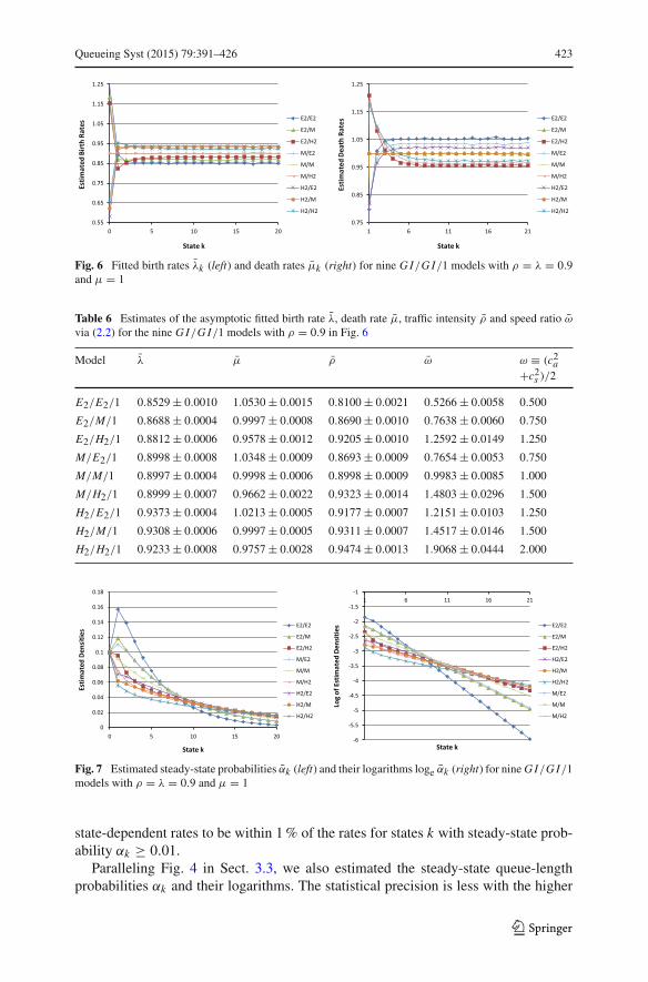
Queueing Syst (2015) 79:391–426 423

Fig. 6 Fitted birth rates λk (left) and death rates μk (right) for nine G I/G I/1 models with ρ = λ = 0.9and μ = 1

Table 6 Estimates of the asymptotic fitted birth rate λ, death rate μ, traffic intensity ρ and speed ratio ω

via (2.2) for the nine G I/G I/1 models with ρ = 0.9 in Fig. 6

Model λ μ ρ ω ω ≡ (c2a

+c2s )/2

E2/E2/1 0.8529 ± 0.0010 1.0530 ± 0.0015 0.8100 ± 0.0021 0.5266 ± 0.0058 0.500

E2/M/1 0.8688 ± 0.0004 0.9997 ± 0.0008 0.8690 ± 0.0010 0.7638 ± 0.0060 0.750

E2/H2/1 0.8812 ± 0.0006 0.9578 ± 0.0012 0.9205 ± 0.0010 1.2592 ± 0.0149 1.250

M/E2/1 0.8998 ± 0.0008 1.0348 ± 0.0009 0.8693 ± 0.0009 0.7654 ± 0.0053 0.750

M/M/1 0.8997 ± 0.0004 0.9998 ± 0.0006 0.8998 ± 0.0009 0.9983 ± 0.0085 1.000

M/H2/1 0.8999 ± 0.0007 0.9662 ± 0.0022 0.9323 ± 0.0014 1.4803 ± 0.0296 1.500

H2/E2/1 0.9373 ± 0.0004 1.0213 ± 0.0005 0.9177 ± 0.0007 1.2151 ± 0.0103 1.250

H2/M/1 0.9308 ± 0.0006 0.9997 ± 0.0005 0.9311 ± 0.0007 1.4517 ± 0.0146 1.500

H2/H2/1 0.9233 ± 0.0008 0.9757 ± 0.0028 0.9474 ± 0.0013 1.9068 ± 0.0444 2.000

Fig. 7 Estimated steady-state probabilities αk (left) and their logarithms loge αk (right) for nine G I/G I/1models with ρ = λ = 0.9 and μ = 1

state-dependent rates to be within 1 % of the rates for states k with steady-state prob-ability αk ≥ 0.01.

Paralleling Fig. 4 in Sect. 3.3, we also estimated the steady-state queue-lengthprobabilities αk and their logarithms. The statistical precision is less with the higher

123

424 Queueing Syst (2015) 79:391–426

traffic intensity ρ = 0.9 instead of ρ = 0.8, as expected from [48]. To illustrate,the estimate of α10 in the H2/M/1 model with ρ = 0.9 was α10 = 0.03251. Thesample standard deviation from the 30 replications was 0.000351. Using the Studentt distribution with 29 degrees of freedom, the t value for a two-sided 95 % confidenceinterval is 2.045. Thus, the halfwidth of the 95 % confidence interval is (2.045 ×0.000351)/

√30 = 0.37340 × 0.000351 = 0.000131, which is less than 0.5 % of the

estimated value (Fig. 7).This is contrasted with the case with traffic intensity ρ = 0.8. The estimate of α10

in the H2(2)/M/1 model with ρ = 0.8 was α10 = 0.02839. The sample standarddeviation from the 30 replications was 0.000282. Using the procedure as above, thehalfwidth of the 95 % confidence interval was found to be 0.000105, which is lessthan 0.4 % of the estimated value, about 0.37 %.

References

1. Abate, J., Choudhury, G.L., Whitt, W.: Waiting-time tail probabilities in queues with long-tail service-time distributions. Queueing Syst. 16, 311–338 (1994)

2. Abate, J., Whitt, W.: A heavy-traffic expansion for the asymptotic decay rates of tail probabilities inmulti-channel queues. Op. Res. Lett. 15, 223–230 (1994)

3. Armony, M., Israelit, S., Mandelbaum, A., Marmor, Y., Tseytlin, Y., Yom-Tov, G.: Patient flow inhospitals: a data-based queueing-science perspective. New York University. Available at http://ie.technion.ac.il/serveng/References/ (2014). Accessed 19 Oct 2014

4. Bhat, U.N., Miller, G.K., Rao, S.S.: Statistical analysis of queueing systems. In: Dshalalow, J.H. (ed.)Frontiers in Queueing Theory, pp. 351–394. CRC Press, Boca Raton, FL (1997)

5. Billingsley, P.: Statistical Inference for Markov Processes. University of Chicago Press, Chicago (1961)6. Bohlin, T.: Practical Grey-Box Process Identification. Springer, London (2006)7. Brown, L., Gans, N., Mandelbaum, A., Sakov, A., Shen, H., Zeltyn, S., Zhao, L.: Statistical analysis

of a telephone call center: a queueing-science perspective. J. Am. Stat. Assoc. 100, 36–50 (2005)8. Buzen, J.: Fundamental operational laws of computer system performance. Acta Inform. 14, 167–182

(1976)9. Buzen, J.: Operational analysis: an alternative to stochastic modeling. In: Ferarri, D. (ed.) Performance

of Computer Installations, pp. 175–194. North Holland, Amsterdam (1978)10. Cerbone, G., Ricciardi, L.M., Sacerdote, L.: Mean, variance and the skewness of the first passage time

for the Ornstein–Uhlenbeck process. Cybern. Syst. 14(2), 395–429 (1981)11. Choudhury, G.L., Whitt, W.: Heavy-traffic asymptotic expansions for the asymptotic decay rates in the

B M AP/G/1 queue. Stoch. Models 10(2), 453–498 (1994)12. Cohen, J.W.: Some results on regular variation for distributions in queueing and fluctuation theory. J.

Appl. Probab. 10(2), 343–353 (1973)13. Cooper, R.B.: Introduction to Queueing Theory, 2nd edn. North Holland, Amsterdam (1982)14. Cox, D.R., Lewis, P.A.W.: The Statistical Analysis of Series of Events. Methuen, London (1966)15. Denning, P.J., Buzen, P.J.: The operational analysis of queueing network models. Comput. Surv. 10,

225–261 (1978)16. Dong, J., Whitt, W.: Stationary birth-and-death processes fit to queues with periodic arrival rate func-

tions. In preparation (2014)17. Duffield, N.G., Whitt, W.: Control and recovery from rare congestion events in a large multi-server

system. Queueing Syst. 26, 69–104 (1997)18. Eick, S.G., Massey, W.A., Whitt, W.: The physics of the Mt /G/∞ queue. Oper. Res. 41, 731–742

(1993)19. El-Taha, M., Stidham, S.: Sample-Path Analysis of Queueing Systems. Kluwer, Boston (1999)20. Fendick, K.W., Whitt, W.: Measurements and approximations to describe the offered traffic and predict

the average workload in a single-server queue. Proc. IEEE 71(1), 171–194 (1989)21. Halfin, S., Whitt, W.: Heavy-traffic limits for queues with many exponential servers. Op. Res. 29(3),

567–588 (1981)

123

Queueing Syst (2015) 79:391–426 425

22. Hastie, T., Tibshirani, R., Friedman, J.: The Elements of Statistical Learning, 2nd edn. Springer, NewYork (2009)

23. Iglehart, D.L.: Limit diffusion approximations for the many-server queue and the repairman problem.J. Appl. Probab. 2, 429–441 (1965)

24. Iglehart, D.L., Whitt, W.: Multiple channel queues in heavy traffic. I. Adv. Appl. Probab. 2(1), 150–177(1970)

25. Iglehart, D.L., Whitt, W.: Multiple channel queues in heavy traffic, II: sequences, networks and batches.Adv. Appl. Probab. 2(2), 355–369 (1970)

26. Keiding, N.: Maximum likelihood estimation in the birth-and-death process. Ann. Stat. 3, 363–372(1975)

27. Kim, S., Whitt, W.: Are call center and hospital arrivals well modeled by nonhomogeneous Poissonprocesses? Manuf. Serv. Op. Manag. 16(3), 464–480 (2014)

28. Kim, S., Whitt, W.: Choosing arrival process models for service systems: tests of a nonhomogeneousPoisson process. Nav. Res. Logist. 17, 307–318 (2014)

29. Kristensen, N.R., Madsen, H., Jorgensen, S.B.: Parameter estimation in stochastic grey-box models.Automatica 40(2), 225–237 (2004)

30. Pakes, A.G.: On the tails of waiting-time distributions. J. Appl. Probab. 12, 555–564 (1975)31. Pang, G., Talreja, R., Whitt, W.: Martingale proofs of many-server heavy-traffic limits for Markovian

queues. Probab. Surv. 4, 193–267 (2007)32. Pang, G., Whitt, W.: Two-parameter heavy-traffic limits for infinite-server queues. Queueing Syst. 65,

325–364 (2010)33. Pang, G., Whitt, W.: The impact of dependent service times on large-scale service systems. Manuf.

Serv. Op. Manag. 14(2), 262–278 (2012)34. Pang, G., Whitt, W.: Two-parameter heavy-traffic limits for infinite-server queues with dependent

service times. Queueing Syst. 73(2), 119–146 (2013)35. Puhalskii, A.A., Reiman, M.I.: The multiclass G I/P H/N queue in the Halfin–Whitt regime. Adv.

Appl. Probab. 32, 564–595 (2000)36. Ross, J.V., Taimre, T., Pollett, P.K.: Estimation for queues from queue-length data. Queueing Syst. 55,

131–138 (2007)37. Ross, S.M.: Stochastic Processes, 2nd edn. Wiley, New York (1996)38. Sigman, K.: Stationary Marked Point Processes: An Intuitive Approach. Chapman and Hall/CRC, New

York (1995)39. Sriram, K., Whitt, W.: Characterizing superposition arrival processes in packet multiplexers for voice

and data. IEEE J. Sel. Areas Commun. SAC–4(6), 833–846 (1986)40. Stone, C.J.: Limit theorems for random walks, birth and death processes and diffusion processes. Ill.

J. Math. 4, 638–660 (1963)41. Thomas, M.U.: Some mean first-passage time approximations for the Ornstein–Uhlenbeck process. J.

Appl. Probab. 12(3), 600–604 (1975)42. Vasilakis, C., Marshall, A.H.: Modelling nationwide hospital length of stay: opening the black box. J.

Op. Res. Soc. 56(3), 862–869 (2005)43. Whitt, W.: Comparing counting processes and queues. Adv. Appl. Probab. 13, 207–220 (1981)44. Whitt, W.: Approximating a point process by a renewal process: two basic methods. Op. Res. 30,

125–147 (1982)45. Whitt, W.: On the heavy-traffic limit theorem for G I/G/∞ queue. Adv. Appl. Probab. 14(1), 171–190

(1982)46. Whitt, W.: Untold horrors of the waiting room. What the equilibrium distribution will never tell about

the queue-length process. Manag. Sci. 29(4), 395–408 (1983)47. Whitt, W.: Departures from a queue with many busy servers. Math. Op. Res. 9(4), 534–544 (1984)48. Whitt, W.: Planning queueing simulations. Manag. Sci. 35(11), 1341–1366 (1989)49. Whitt, W.: Understanding the efficiency of multi-server service systems. Manag. Sci. 38(5), 708–723

(1992)50. Whitt, W.: Stochastic-Process Limits. Springer, New York (2002)51. Whitt, W.: A diffusion approximation for the G/G I/n/m queue. Op. Res. 52(6), 922–941 (2004)52. Whitt, W.: Engineering solution of a basic call-center model. Manag. Sci. 51, 221–235 (2005)53. Whitt, W.: Staffing a call center with uncertain arrival rate and absenteeism. Prod. Op. Manag. 15(1),

88–102 (2006)54. Whitt, W.: Fitting birth-and-death queueing models to data. Stat. Probab. Lett. 82, 998–1004 (2012)

123

426 Queueing Syst (2015) 79:391–426

55. Whitt, W.: Heavy-traffic limits for queues with periodic arrival rates. Op. Res. Lett. 42, 458–461 (2014)56. Whitt, W.: The steady-state distribution of the Mt /M/∞ queue with a sinusoidal arrival rate function.

Op. Res. Lett. 42, 311–318 (2014)57. Wolff, R.W.: Problems for statistical inference for birth and death queueing models. Op. Res. 13,

343–357 (1965)58. Wolff, R.W.: The effect of service-time regularity on system performance. In: Chandy, K.M., Reiser,

M. (eds.) Comput. Perform., pp. 297–304. North-Holland, Amsterdam (1977)59. Yin, L., Uttamchandani, S., Katz, R.: An empirical exploration of black-box performance models for

storage systems. In: Proceedings of the 14th IEEE International Symposium on Modeling, Analysis,and Simulation of Computer and Telecommunication Systems, MASCOTS 2006. IEEE, pp. 433–440(2006)

123