solving a real-world supply-chain management problem using ...kdeb/papers/c2017009.pdf · solving a...

Solving a Real-world Supply-Chain ManagementProblem Using a Bilevel Evolutionary Approach

COIN Report Number 2017009

Zhichao Lua, Kalyanmoy Deba, Erik Goodmana, John Wassickb

aMichigan State UniversitybThe Dow Chemical Company

Abstract

Supply-chain management problems are common to most industries andthey involve a hierarchy of subtasks, which must be coordinated well toarrive at an overall optimal solution. Such problems also involve more thanone stake-holders, such as the supplier, the transport companies that supplygoods from source to destinations, and multiple management levels withinthe supplier. Thus, these problems involve a hierarchy of decision-makers,each having its own objectives and constraints, but importantly requiringa coordination of their actions to make the overall supply chain processoptimal from cost and quality considerations. In this paper, we considera specific supply-chain management problem from an industry, which in-volves two levels of coordination: (i) yearly strategic planning in whicha decision on establishing an association of every destination point witha supply point must be made so as to minimize the yearly transportationcost, and (ii) weekly operational planning in which, given the associationbetween a supply and a destination point, a decision on the preference ofavailable transport carriers must be made for multiple objectives: minimiza-tion of transport cost and maximization of service quality and satisfactionof demand at each destination point. Thus, the resulting problem is bilevel,for which the operational planning problem is nested within the strategicplanning problem. The problem is also multi-objective in nature. Moreover,the problem involves several practical challenges, such as uncertainty indemand at each destination, non-linearity and non-differentiability of thecost model, large dimensions, and others. We propose a customized multi-objective bilevel evolutionary algorithm, which is computationally tractable.We then present results on state-level and ZIP-level accuracy (involvingabout 40,000 upper level variables) of destination points over the mainland

USA. We compare our proposed method with current non-optimizationbased practices and report a considerable cost saving.

1. Introduction

Supply chain management (SCM) problems are common in most inte-grated industries, as a product is made from several raw or pre-finishedsub-products and the product itself, after being produced, must be trans-ported to several destination locations. SCM problems come in differentcomplexities and involve multiple goals, such as minimizing transportationcost, adhering to scheduled delivery time, maximizing service quality, etc.Importantly, different sub-tasks are hierarchical and interconnected. Thus,it is not surprising that SCM problems are often treated as optimizationproblems [1, 8, 15].

In this paper, we consider a particular routine SCM problem in which aproduct needs to be supplied from multiple source locations (manufacturingplants or warehouses) to several destinations across mainland US states andZIP locations. The task is considered routine, as the product needs to besupplied according to a given demand every week for an entire year at eachdestination location. The task is hierarchical having at least two levels. Thestrategic level task is to identify (i) an association of each destination locationwith a specific source location and also (ii) an assignment of a set of transportcarrier companies with each source location. The strategic task is done lessfrequently, may be once a year. For a specific combination of these twosub-tasks fixed for the entire year, every source location is then aware of thedestination locations where the product needs to be supplied to and alsothe carrier companies that will deliver the products. Then, at the operationallevel, a decision needs to be made to allocate an optimal proportion of dailydemand to be transported by a carrier company to every destination location.This task needs to be done more frequently, may be once every week ordaily. Thus, the operational (or lower) level task has as many optimizationproblems as the source locations. At the strategic (or upper) level, there isan overriding objective of minimizing the overall transportation cost fordelivering products from every source to every destination location. Atthe lower level, there can be a single or two objectives: (i) minimizing thetransport cost associated with every source location for completing thedelivery task to all its associated destination locations, and (ii) maximizinga service quality of all carrier companies chosen to deliver the product fromthe specific source location. A little thought will reveal that this problem is a

2

bilevel optimization problem involving a single objective at the upper leveland at most two objectives at the lower level. The problem is more complexthan an usual bilevel optimization problem, as the lower level task involvesmultiple optimization problems in parallel.

Bilevel optimization is commonly characterized as a mathematical pro-gramming problem that involves two nested levels of optimization. Theouter problem is usually denoted as the upper level optimization task andthe inner optimization task is usually denoted as the lower level problem. Inthe are of game theory, bilevel optimization problems were first introducedby Stackelberg [12] and came to be known as Stackelberg games; ThenBracken and McGill [2] from the area of mathematical programming laterpresented bilevel problems as a constrained optimization task, in which thelower level optimization problem acts as a constraint to the upper level opti-mization problem. The interest in bilevel programming has been driven bya number of applications arising in the field of operation research, includingtransportation [10, 4, 3], management [13], facility location [7, 14, 13]. Overthe past few years, evolutionary computation (EC) has become a promis-ing mean in solving bilevel optimization problems because of its flexibleframework and population approach, offer viable means to address the com-plexities that are otherwise difficult to handle using classical optimizationtechniques.

In this paper, we develop bilevel evolutionary optimization methodsto solve single and multi-objective version of the above-mentioned SCMproblem. The study is also significant as after considering one state-leveldestination location, we have considered ZIP-level destination locations,involving about 40,000 nodes. This consideration increases the problem sizeby 1,000-fold and makes the overall bilevel programming task challenging.Moreover, one of the trade-mark challenges of SCM problems is that demandto each destination is usually uncertain and that demand changes weeklyand seasonally. We have considered demand uncertainties as well andinvestigated its effect in arriving at robust solutions of the problem. With allthese considerations, this study brings evolutionary computation close toreal-world application of a routine supply chain management problem.

In the remainder of this paper, the specific supply chain managementproblem is described in Section 2. Details of source and destination loca-tions and associated transport carriers are mentioned as well. Thereafter, inSection 3, we formulate the SCM problem as a bilevel optimization problem.Section 4 describes the evolutionary bilevel optimization procedure devel-oped for solving the SCM problem. Then, Section 5 presents the simulationresults for both single-objective and multi-objective bilevel versions of the

3

SCM problem. Advantages of using the multi-objective version is also de-scribed in this section. Thereafter, in Section 6, the demand uncertainty isconsidered and results are shown. The difference between robust solutionsand deterministic solutions are then highlighted. Section 7 discusses themodified algorithm for handling ZIP-level destination locations, therebyaddressing a large-scale version of the SCM problem. Finally, Section 8concludes this extensive study.

2. Problem Description and Modeling

Figure 1: An example of the upper level problem showing destination (states) to sourcelocation associations.

The supply chain management problem with two levels of interactionsis described in Figure 1. We provide more details of the problem in thefollowing subsections.

2.1. Source Locations and Their CharacteristicsIn total, 10 source locations all over mainland USA are considered, as

shown in Table 1. Each source location is considered to have infinite capacity,so that any quantity of product can be supplied from each source. Here, we

4

Table 1: Ten assumed source locations.

Location # City State Abbrev.1 Saint Louis MO StL2 Los Angeles CA LA3 Augusta GA AUG4 New Orleans LA NOR5 Detroit MI DET6 Minneapolis MN MIN7 Charlotte NC CHA8 Philadelphia PA PHI9 Houston TX HOU

10 Seattle WA SEA

also assume that a single product is supplied from all source locations to alldestination locations.

2.2. Destination Locations and Their Demand ModelingWe consider two scenarios related to destination locations. In the first

scenario, we consider one destination location at the capital city of everystate, thereby making 48 different destination locations all over mainlandUSA. In the second scenario (discussed in Section 7, we have consideredone location at every ZIP level, thereby making a total 40,000 destinationlocations. At each location, following parameters are chosen based onrealistic data obtained from a particular industry:

• A yearly average demand is set to be 42,400 in shipments.

• The demand at each destination location is proportional to its popula-tion statistics.

• Two types of demands are considered, seasonal and non-seasonal.

A deterministic or fixed demand example is provided in Figure 2 for somestates. In the event of demand being uncertain (considered in Section 6), thedemand changes from week to week.

2.3. Transport Carrier ModelingAt each source, five competitive transport carriers are regularly contract-

ed to fulfill the anticipated demand. And we assume additional transportcarriers with willingness to take any volume are always available with 25%

5

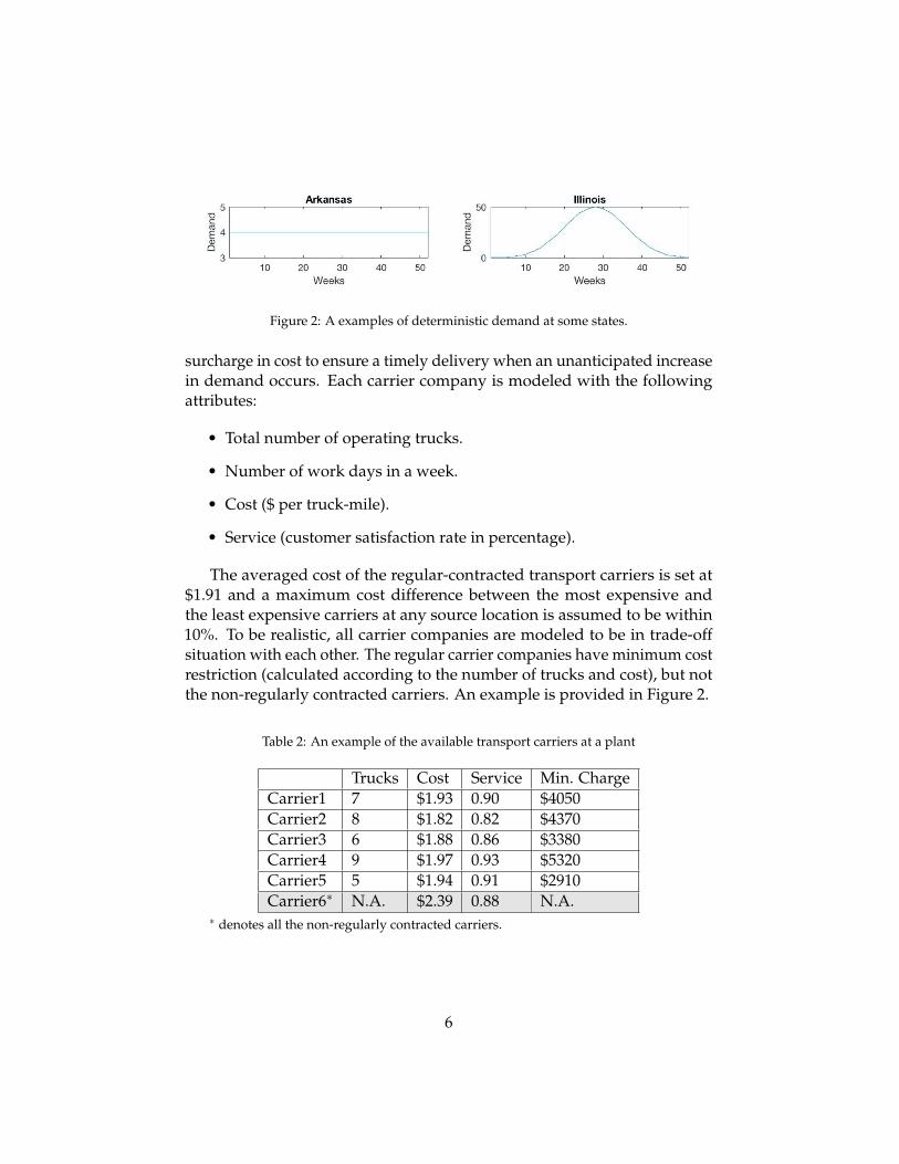
Figure 2: A examples of deterministic demand at some states.

surcharge in cost to ensure a timely delivery when an unanticipated increasein demand occurs. Each carrier company is modeled with the followingattributes:

• Total number of operating trucks.

• Number of work days in a week.

• Cost ($ per truck-mile).

• Service (customer satisfaction rate in percentage).

The averaged cost of the regular-contracted transport carriers is set at$1.91 and a maximum cost difference between the most expensive andthe least expensive carriers at any source location is assumed to be within10%. To be realistic, all carrier companies are modeled to be in trade-offsituation with each other. The regular carrier companies have minimum costrestriction (calculated according to the number of trucks and cost), but notthe non-regularly contracted carriers. An example is provided in Figure 2.

Table 2: An example of the available transport carriers at a plant

Trucks Cost Service Min. ChargeCarrier1 7 $1.93 0.90 $4050Carrier2 8 $1.82 0.82 $4370Carrier3 6 $1.88 0.86 $3380Carrier4 9 $1.97 0.93 $5320Carrier5 5 $1.94 0.91 $2910Carrier6∗ N.A. $2.39 0.88 N.A.

∗ denotes all the non-regularly contracted carriers.

6

3. A Bilevel Formulation of the SCM Problem

We present the bilevel formulation of the SCM management problemin Equation 1 and the notations used in the formulation are presented inTable 3.

Min. F(x, y) = ∑m

∑n

fm,n(x, y),

s.t. y ∈ argmin{

fm,n(x, y) =c

∑j=1

f′j (x, yj) |,

d

∑i=1

wi · yij ≤ Cj, i = 1, . . . , d(estinations),

c

∑i=j

yij = Di, j = 1, . . . , c(arriers),

f′j (x, yj) = max(

d

∑i=1

DDi(x) · yij · CCj, τj)}

,

m = 1, 2, . . . , p(lants), n = 1, 2, . . . , 52 weeks.

(1)

Table 3: Notation Used In The Proposed Bilevel Formulation

Symbols

x: source-to-destination associationy: demand fulfillment matrixw: days need for a round tripτ: carrier minimum chargeC : carrier capacityCC: carrier costD: demandDD: driving distance

4. Proposed Algorithm

Finding an optimal source-to-destination association mapping involvestwo levels of interactive optimization of integer variables, which makesthe problem given in Equation 1 a bilevel integer non-linear programming

7

problem [9]. Bilevel programming (or Stackelberg game) has become anincreasingly popular framework in solving supply-chain management typeproblems and researchers have used both approximated and nested methodsto handle the problem in different applications. These two strategies havetheir own advantages and disadvantages. An meta-model based approachmight be computationally tractable, but does not, in most cases, guaranteeoptimality. On the other hand, an exact method would guarantee optimalitywith certain assumptions, but might be computational intractable for manyreal-world application scale problems.

In the remainder of this section, we describe a nested bilevel approachwhich is customized to solve this SCM problem. The supplying decisions (x)is determined at the strategic level (upper level) of our solution procedurethat assigns a supplying plant index to every demand destination. Oncethe supplying decision is fixed, at the operational level (lower level) wedetermine the corresponding optimal delivery decision (y) at each timestage. A population-based method is used to generate supplying strategiesat the upper level and the corresponding optimal delivery strategies areobtained by solving a non-linear integer programming problem at the lowerlevel.

Algorithm 1: Upper level initialization procedure.Input: population size (N)Output: population (P)

1 Initialize P← ∅, i← 02 for indvIndex < N do3 for destinationIndex < length(indv) do4 Sort driving distance (DD) from each plant m to each

destination i in ascending order.5 The probability of supplying i destination from plant m is :

6 prob. ← DD from m to isum(top 5 DD)

7 Assign indv(destinationIndex) based on the above prob.8 end9 P(indvIndex)← indv

10 end11 return P

A population-based method uses principles from biological evolution todrive the population towards the optimum by generating offsprings from

8

genetic operations (crossover and mutation). The proposed solution methodprogresses in a nested manner and two different population-based optimiza-tion algorithms are used at the two levels. To improve the convergenceefficiency of the proposed algorithm, a customized initialization (describedin Algorithm 1) is introduced in the upper level. The lower level population-based algorithm uses customized recombination and mutation operatorsthat are recently proposed by Deb et al. (details can found at [5]). A variancebased stopping criteria (as described in Equation 2) is used for terminationat both level, as shown below:

αT = ∑ni=1 σ2(xi)|T

∑ni=1 σ2(xi)|0

. (2)

When the value of αT at any generation T becomes less than αstop thenthe algorithm terminates. In the above equation, n is the number of upperlevel variables, σ2(xi)|T is the variance across dimension i at generation Tand σ2(xi)|0 is the variance across dimension i in the initial population.

The proposed algorithm has been implemented in MATLAB. The param-eters used in the algorithm are:

1. λ = 2 (offsprings created at each generation),2. r = 2 (individuals updated at each generation),3. N = 48 (upper level population size),4. n = 48 (lower level population size),5. αstop = 0.001.

5. Experiments Setup and Empirical Results

In this section, we present the empirical results obtained from using theproposed bilevel formulation of the SCM problem with the demand andcarrier models described in section 3. We first compare it with the common-practice strategy, which is a simplified single-level model that overlooksthe delivery planning stage by averaging over the available carriers. Tosimulate the performance of this single-level model, we use a randomassignment method to replace the optimization process in the operationallevel. We then enhance our model and proposed algorithm to handle variouspracticalities including multiple objectives in the operational level planning,robust solution under demand uncertainties, and a large scale destinations.The results are presented in the following part of this section.

9

5.1. State-Level Destination LocationsThe initial experiment is conducted on a restricted destinations in which

we limit the possible demand destinations to state level (the lower 48 states).We then use state capitols to calculate the driving distances from supplyingsource locations. A simulation result over one year (52 weeks) comparingsingle-level and our bilevel model is provided in Table 4, with savingsprovided in the parentheses.

Table 4: Yearly Transportation Cost Comparison on State-level Destinations.

Model Single-level Bilevel

Transportation Cost $ 16.2M $ 15.5M (4.3%)

Figure 3: An example of state level destination bilevel solution.

It is worth to note that the resulting source-to-destination associations, asshown in Figure 3, in the strategic level are identically the minimum drivingdistance strategy from both models. The source locations are marked on themap with corresponding color indicating the supplying destinations in statelevel. One instance of the optimized delivery strategy in the operationallevel for the plant at Saint Louis in week 32 from our bilevel model isprovided in Table 7. The related model information is also provided inTable 5 and 6.

10

Table 5: Demand destinations serving from the plant at Saint Louis.

Destinations AR IL KS KY MO TNRound Trip Days 2 1 2 2 1 2

Table 6: The available transport carriers of Plant At Saint Louis

Trucks Cost Service Min. ChargeCarrier1 6 $1.86 0.85 $3350Carrier2 7 $1.89 0.87 $3970Carrier3 7 $1.92 0.89 $4030Carrier4 7 $1.96 0.92 $4120Carrier5 6 $1.85 0.84 $3330Carrier6 N.A. $2.39 0.88 N.A.

Table 7: Cost-optimal delivery strategy from operational level optimization of plant at SaintLouis in week 32.

Ar IL KS KY MO TN Occ. Cap.Carrier1 0 4 0 0 12 13 42 42Carrier2 0 23 0 0 15 17 23 49Carrier3 0 0 0 0 0 0 0 49Carrier4 0 0 0 0 0 0 0 49Carrier5 0 0 6 9 0 0 42 42Carrier6 0 0 0 0 0 0 0 N.A.Supply 6 27 6 9 12 13 Tran. CostDemand 6 27 6 9 12 13 $29,880

11

5.2. Multiple Objectives at the Operation LevelThe supply-chain management in practice most often has multiple con-

flicting goals arising from economic, environmental and efficiency-relatedissues. Similarly in this problem, a second objective of maximizing theservice quality at the operational level is essential from the practical per-spective. Hence, a multi-objective optimization method is a ideal way offirst finding a set of trade-off Pareto-optimal solutions and then choosinga preferred solution based on the multi-criterion decision analysis. We usethe carrier service quality rate (CS) described in Section 2 to formulate thesecond objective, the service quality, as below:

f (2)m,n(x, y) =c

∑j=1

d

∑i=1

yij · CSj. (3)

We then incorporate the non-dominated sorting and crowding distancetechnique proposed in [6] to assign fitness in the operational level opti-mization. Now a set of trade-off solutions are preserved at the end of eachoperational level optimization, and we use the same example in the previoussubsection to illustrate.

Figure 4: Pareto-optimal trade-offs between transportation cost and service quality of sourceat Saint Louis in week 32.

The Figure 4 presents a set of Pareto-optimal solutions that shows thetrade-off between transportation cost and service quality of the plant at

12

Saint Louis in week 32. The delivery strategy represented by one of theextreme point that minimize the transportation cost is the same as the resultsshown in Table 7 in the previous subsection, as expected. We also providethe delivery strategy details of one intermediate solution in Table 8 and theother extreme solution that maximize the service quality in Table 9.

Table 8: Intermediate trade-off solution from Figure 4.


Table 9: The best service quality solution from Figure 4.


The main difference among these three Pareto-optimal solutions is thenumber of shipments assigned to the Carrier4, which provides the bestservice quality among the five available transport carriers at a premiumprice. A gain of 5% improvement in service quality costs an increase of$1,170 in weekly transportation for the plant at Saint Louis to switch froma transportation cost prioritized delivery strategy to a service prioritizedstrategy. The overall strategic level planning solution from bi-objective op-erational level planning remains the same as the minimum driving distance

13

strategy solution shown in Figure 3. The operational level decision is madeon random-basis for simulation purpose and a more sophisticated decisionmaking procedure can be easily incorporated into our proposed algorithm.The results are summarized in Table 10.

Table 10: Yearly transportation cost and service quality comparison for state-level destina-tions.

Model Single-objective Bi-objective

Transportation Cost $ 15.5M $ 15.9M

Service Quality∗ 0.86 0.89

∗An averaged service quality in percentage from operational level.

6. Robust SCM Solutions Under Demand Uncertainty

The uncertain demand (demanduncer) that may arise in our bilevel for-mulation is modeled with a Gaussian random variable with the anticipateddemand being the mean and a variance controlled by the parameter σ, asshown below:

demanduncer = demand + σ · demand · N(0, 1), (4)

where N(0, 1) denotes a normal random variable. An example of the re-sulting uncertain seasonal as well as non-seasonal demands are providedrespectively in Figure 5 and 6.

To account for the uncertainties that may arise in demands, the oper-ational level procedure in our proposed algorithm has been modified tofirst collect samples from the corresponding demand random variable, thenoptimize against each of the collected samples and then take an averageof the objectives in the end of the process for subsequent calculation. Forthe purpose of demonstrating the proposed method, we run the simulationusing our bilevel model with single objective (transportation cost) in theoperational level. And we introduce uncertainties in all the state-level desti-nations and our proposed robust solution procedure has found the optimalstrategic level decision with σ = 0.1 as shown in Figure 7.

To further analyze the sensitivity of the results obtained from our pro-posed robustness-based solution procedure, we run 11 trials of re-evaluating

14

Figure 5: Seasonal demand with uncertain-ties.

Figure 6: Non-seasonal demand with uncer-tainties.

Figure 7: The strategic level decision under 10% demand uncertainties.

the deterministic optimal strategic level decision (presented in Section 5.1)with uncertain demands at all state-level destinations, we then compare theresults with the robust optimal strategic level decision in different σ settings.Table 11 records the minimum, median, and maximum transportation costfrom the 11 trials of the experiment and Figure 8 provides a visualization ofthe results.

It is clear from both Table 11 and Figure 8 that the robust solutions fromour proposed method have a smaller variance in the objective functionvalues compared to the same for the deterministic solution. This indicatesthe importance of a robust optimal strategy in making a relatively insensitivesolution to the uncertainties in demand values. However, the lower varianceoccurs with a minor sacrifice in the median objective function value. It is

15

Table 11: Robust and Deterministic Solution Comparison on Yearly Transportation Cost

σ = 0.05 σ = 0.1 σ = 0.15MIN MED MAX MIN MED MAX MIN MED MAX

Determ. $14.3M $15.5M $16.1M $13.9M $15.6M $16.6M $13.6M $15.5M $16.9MRobust $14.2M $15.6M $16.0M $14.1M $15.9M $16.3M $13.9M $15.8M $16.5M

Figure 8: Robust and Deterministic Solution Comparison on Yearly Transportation Cost

now a matter of higher-level management decision whether the trade-offbetween robustness in terms of a more stable objective value (transport cost)and the increase in objective value is acceptable to the specific industry ornot.

We now discuss the qualitative differences between the deterministicand robust solutions obtained with different σ values in demand.

• For a 5% uncertainty in demand, there is no difference in the source-destination allocation between deterministic and robust solutions. Theuncertainty is too small to keep the deterministic solution to be robust.

16

• However, when a 10% or more uncertainty in demand is considered,the robust upper level solution re-assigns VA state to Plant at CHAfrom Plant at PHI, which was assigned in the deterministic upperlevel solution. The uncertainty level is large enough to make thedeterministic solution brittle.

There are differences in the lower level solutions between deterministic androbust solutions, thereby causing the differences in the overall transportcost, as shown in Table 11.

7. Large-Scale Version of the SCM Problem

Until now, this paper has restricted the demand destinations to statelevel to make our bilevel model and the proposed algorithm computation-ally tractable. Unfortunately, the demand in practice could come from anyof the ZIP locations in the country. Hence, to tackle this problem, we firstperformed a post-optimal analysis on the optimal single objective (trans-portation cost) operational level decision with the state level destinationsand two important rules have been extracted, as shown below:

• The cheaper transport carriers should be completely assigned.

• Long-distance delivery should be assigned to cheaper transport carri-ers with priority.

We then use these two rule-based delivery strategy to approximate thereaction function (Ψ) of the operational level optimal decision, instead ofrunning an optimization algorithm at this level. The upper level problem isstill solve using an EA. This idea falls in the category of derived heuristicsbased optimization proposed recently in another context [11]. We re-writethe original bilevel formulation presented in Equation 1 as below (g(x, y)denotes all constraints):

min F(x, y),s.t. y ∈ Ψ(x),

Ψ(x) = argmin{ f (x, y)|g(x, y) < 0}.(5)

One instance of the operational level solution with ZIP-code destinationsof the plant at Saint Louis is provided in Figure 9. The respective strategiclevel decision is provided in Figure 10. These figures shows that ZIP levelassociation is now made independent of state boundaries, thereby reducingthe overall transport cost of solving the SCM problem from $ 15.5M to $15.2M.

17

Figure 9: Optimized operational level decision of the source at Saint Louis.

Figure 10: Optimized strategic level decision with ZIP-level destinations.

8. Conclusions

This paper has considered a specific supply chain management problemmotivated by discussions and data obtained from an integrated industry.

18

The SCM problem is hierarchical, having two levels of management consid-erations – (i) strategic decisions which are performed yearly to decide onglobal SCM parameters such as association of destination locations with aspecific supply location and assignment of transport carrier companies toeach supply location, and (ii) operational decisions which are performedweekly to decide on the extent of the use of each carrier company at eachsupply location for every week. The resulting bilevel problem has beensolved using a customized bilevel optimization algorithm for single andmultiple objectives at operational level. Results from bilevel considerationhave shown to have about 4% reduction in overall cost of operation com-pared to a single-level optimal solution. When both transport cost andservice quality of carrier companies are used two objectives at the oper-ational level, the multi-objective bilevel algorithm is able to find a betterservice quality solution with a slightly increased transport cost.

Following the deterministic demand scenario, the SCM problem hasbeen made more realistic by considering uncertainty in the weekly demandat each destination location. A robust bilevel procedure has been usedand the resulting robust solution has been shown to have a more stableoverall transport cost compared to a large fluctuation observed with thedeterministic solution.

Finally, to make the SCM problem more realistic, the original single-objective bilevel SCM problem is extended to include the large-scale version(ZIP-level). It has been observed that a supply location may now get associ-ated with ZIP locations from multiple states, thereby providing a reducedoverall transport cost.

The study is significant from the algorithmic point of view, as well. Con-sideration of state-level (small size) to ZIP-level (large size), deterministicto uncertainty-based demand, single to multiple conflicting objectives, andsingle to bilevel optimization in the SCM problem make the study close topractice. The study has also shown the flexibility of evolutionary algorithmsto handle all such challenges faced in a specific real-world SCM problem.

Acknowledgements

Authors acknowledge the support provided by MSU Midland ResearchInstitute for Value Chain Creation (MRIVCC) and The Dow Chemical Com-pany for executing this study.

19

References

[1] Fulya Altiparmak, Mitsuo Gen, Lin Lin, and Turan Paksoy. A geneticalgorithm approach for multi-objective optimization of supply chainnetworks. Computers & industrial engineering, 51(1):196–215, 2006.

[2] J. Bracken and J. McGill. Mathematical programs with optimizationproblems in the constraints. Operations Research, 21:37–44, 1973.

[3] Luce Brotcorne, Martine Labbe, Patrice Marcotte, and Gilles Savard. Abilevel model for toll optimization on a multicommodity transportationnetwork. Transportation Science, 35(4):345–358, 2001.

[4] Isabelle Constantin and Michael Florian. Optimizing frequencies ina transit network: a nonlinear bi-level programming approach. In-ternational Transactions in Operational Research, 2(2):149 – 164, 1995.ISSN 0969-6016. doi: http://dx.doi.org/10.1016/0969-6016(94)00023-M. URL http://www.sciencedirect.com/science/article/pii/096960169400023M.

[5] Kalyanmoy Deb and Christie Myburgh. Breaking the Billion-VariableBarrier in real-world optimization using a customized evolutionary algorithm,pages 653–660. Association for Computing Machinery, Inc, 7 2016. doi:10.1145/2908812.2908952.

[6] Kalyanmoy Deb, Samir Agrawal, Amrit Pratap, and T. Meyarivan. Afast and elitist multiobjective genetic algorithm: NSGA-II. IEEE Trans.Evolutionary Computation, 6(2):182–197, 2002. doi: 10.1109/4235.996017.URL http://dx.doi.org/10.1109/4235.996017.

[7] Qin Jin and Shi Feng. Bi-level simulated annealing algorithm for facilitylocation. Systems Engineering, 2:007, 2007.

[8] Douglas M Lambert, Martha C Cooper, and Janus D Pagh. Supplychain management: implementation issues and research opportunities.The international journal of logistics management, 9(2):1–20, 1998.

[9] Duan Li and Xiaoling Sun. Nonlinear integer programming, volume 84.Springer Science & Business Media, 2006.

[10] Athanasios Migdalas. Bilevel programming in traffic planning: Models,methods and challenge. Journal of Global Optimization, 7(4):381–405,1995. ISSN 0925-5001. doi: 10.1007/BF01099649.

20

[11] C. Myburgh and K. Deb. Derived heuristics based consistent optimiza-tion of material flow in a gold processing plant. Engineering optimization,in press.

[12] Heinrich von Stackelberg. The theory of the market economy. OxfordUniversity Press, New York, 1952.

[13] Huijun Sun, Ziyou Gao, and Jianjun Wu. A bi-level programmingmodel and solution algorithm for the location of logistics distributioncenters. Applied Mathematical Modelling, 32(4):610 – 616, 2008. ISSN0307-904X.

[14] Takeshi Uno, Hideki Katagiri, and Kosuke Kato. An evolutionarymulti-agent based search method for stackelberg solutions of bilevelfacility location problems. International Journal of Innovative Computing,Information and Control, 4(5):1033–1042, 2008.

[15] Fan Wang, Xiaofan Lai, and Ning Shi. A multi-objective optimizationfor green supply chain network design. Decision Support Systems, 51(2):262–269, 2011.

21

solving a real-world supply-chain management problem using ...kdeb/papers/c2017009.pdf · solving a...

Documents