rr 427 pavement thickness design charts derived …...pavement thickness design charts derived from...
TRANSCRIPT

Pavement thickness design charts derived from a rut depth finite element model
November 2010
Dr Greg Arnold, Pavespec Ltd
Dr Sabine Werkmeister, University of Canterbury
NZ Transport Agency research report 427

ISBN 978-0-478-37130-7 (print)
ISBN 978-0-478-37129-1 (electronic)
ISSN 1173 3756 (print)
ISSN 1173-3764 (electronic)
NZ Transport Agency
Private Bag 6995, Wellington 6141, New Zealand
Telephone 64 4 894 5400; facsimile 64 4 894 6100
www.nzta.govt.nz
Arnold, G1 and S Werkemeister2 (2010) Pavement thickness design charts derived from a rut depth finite
element model. NZ Transport Agency research report no.427. 84pp.
1 Pavespec Ltd, PO Box 570, Drury 2247, New Zealand (www.rltt.co.nz)
2 Technische Universität Dresden, Mommsenstraße 13, 01069 Dresden, Germany
This publication is copyright © NZ Transport Agency 2010. Material in it may be reproduced for personal
or in-house use without formal permission or charge, provided suitable acknowledgement is made to this
publication and the NZ Transport Agency as the source. Requests and enquiries about the reproduction of
material in this publication for any other purpose should be made to the Research Programme Manager,
Programmes, Funding and Assessment, National Office, NZ Transport Agency, Private Bag 6995,
Wellington 6141.
Keywords: aggregates, basecourse, deformation, pavement design, rut depth prediction, unbound
granular, repeated load triaxial, rutting, specifications for aggregates.

An important note for the reader
The NZ Transport Agency is a Crown entity established under the Land Transport Management Act 2003.
The objective of the Agency is to undertake its functions in a way that contributes to an affordable,
integrated, safe, responsive and sustainable land transport system. Each year, the NZ Transport Agency
funds innovative and relevant research that contributes to this objective.
The views expressed in research reports are the outcomes of the independent research, and should not be
regarded as being the opinion or responsibility of the NZ Transport Agency. The material contained in the
reports should not be construed in any way as policy adopted by the NZ Transport Agency or indeed any
agency of the NZ Government. The reports may, however, be used by NZ Government agencies as a
reference in the development of policy.
While research reports are believed to be correct at the time of their preparation, the NZ Transport Agency
and agents involved in their preparation and publication do not accept any liability for use of the research.
People using the research, whether directly or indirectly, should apply and rely on their own skill and
judgement. They should not rely on the contents of the research reports in isolation from other sources of
advice and information. If necessary, they should seek appropriate legal or other expert advice.

Acknowledgements
The authors would like to acknowledge the assistance provided by Stevenson Laboratory, Winstone
Aggregates and CAPTIF staff in providing data.
Abbreviations and acronyms
AASHTO American Association of State Highway and Transportation Officials
ASR alkali-silica reaction
CalTrans California Department of Transportation
CAPTIF Canterbury accelerated pavement testing indoor facility
CBR California bearing ratio
DOS degree of saturation
ESA equivalent standard axle pass
FE finite element
HMA hot mix asphalt
MDD maximum dry density
MESA millions of equivalent standard axles
NZTA New Zealand Transport Agency
OMC optimum moisture content
RLT repeated load triaxial
Transit NZ Transit New Zealand
UCS unconfined compressive strength
VSD vertical surface deformation (a measurement of rutting)

5
Contents
Executive summary ................................................................................................................................................ 7
Abstract ...................................................................................................................................................................... 8
1 Introduction .................................................................................................................................................. 9
1.1 Background current pavement design method ..................................................... 9
1.2 Observations at the Canterbury accelerated pavement testing indoor facility
(CAPTIF) ............................................................................................................... 11
1.3 Models to predict pavement rutting ...................................................................... 12
1.4 Other models to predict rutting ............................................................................ 12
1.5 Repeated load triaxial tests to obtain parameters for rut depth models ................. 17
2 Rut depth prediction methods ........................................................................................................... 19
2.1 Arnold (2004) rut depth prediction method .......................................................... 19
2.1.1 Introduction ............................................................................................ 19
2.1.2 RLT tests ................................................................................................. 19
2.1.3 Modelling permanent strain ..................................................................... 20
2.1.4 Calculating pavement rut depth ............................................................... 23
2.2 Description of Werkmeister model........................................................................ 24
2.2.1 Modelling the steady state phase using RLT test results ........................... 24
2.2.2 Modelling of post-construction compaction using CAPTIF test results ...... 28
2.2.3 Model validation comparing laboratory results with CAPTIF test results .... 29
2.2.4 Discussion ............................................................................................... 31
3 Repeated load triaxial testing ............................................................................................................ 33
3.1 Introduction ......................................................................................................... 33
3.2 RLT test results for basecourse and sub-base aggregates ..................................... 33
3.3 RLT test results for subgrade soils ....................................................................... 34
4 Rut depth prediction CAPTIF pavements validation Arnold method ........................ 36
5 Rut depth prediction other pavements Arnold method .................................................... 39
6 Granular pavement design charts based on rut depth prediction Arnold method ... 45
7 Granular pavement design charts based on rut depth prediction Werkmeister
method......................................................................................................................................................... 50
8 Comparing the Arnold and Werkmeister methods for determining pavement
thickness design charts ........................................................................................................................ 52
9 Conclusions ............................................................................................................................................... 55
10 Recommendations ................................................................................................................................... 59
11 References .................................................................................................................................................. 60
Appendix A Repeated load triaxial test summary for subgrade soils ..................................... 63
Appendix B Repeated load triaxial testing and rut depth modelling technical note ......... 72
Appendix C Recommended additions to the New Zealand supplement to the 2004
Austroads pavement design guide ................................................................................ 74
Appendix D Method to determine vertical compressive strain criterion from repeated
load triaxial test data .......................................................................................................... 80

6

7
Executive summary
Repeated load triaxial (RLT) tests on subgrade, subbase and basecourse materials enabled relationships to
be determined between permanent strain/rutting and stress (Arnold method) or elastic strain (Werkmeister
method). Through these relationships it was possible to calculate the rutting within each pavement material,
which was then summed to obtain a surface rut depth. The assumptions used to calculate the surface rut
depths to ensure they were close to measured rut depths were validated and refined at the Canterbury
accelerated pavement indoor testing facility (CAPTIF). The validated Arnold and Werkmeister rut depth
prediction models were then used to calculate rutting for a range of pavement depths on subgrade soils with
California bearing ratios (CBRs) of 2%, 8% and 10%. Results of this analysis were assessed by the number of
equivalent standard axle passes (ESAs) to achieve a total surface rut depth defining the end of life. This
information was used to develop pavement thickness design charts from the rut depth predictions and these
were compared to the chart for granular pavements in the Austroads design guide (Austroads 2004, figure
8.1). For low traffic volumes the rut depth model required thinner pavements than the Austroads guide while
for high traffic volumes the rut depth predictions showed significantly thicker pavements were required. In
fact, the rut depth predictions showed that traffic loading limits for granular pavements were around
7 million ESAs for the subgrade CBR 2% and 11 million ESAs for the subgrade CBR 8%. A reason for this was
the significant amount of rutting that occurred in the aggregate layers for the thicker pavement depths. As
rutting occurred within the granular layers, adding more granular material did not decrease the amount of
rutting nor increase pavement life.
Rut depth predictions were repeated with different quality aggregates in terms of resistance to rutting found
from the RLT test at optimum moisture content in drained conditions. The effect of using very good
unbound aggregates increased the maximum pavement life from 11 million ESAs for average quality to
14 million ESAs for a subgrade with CBR 8%. However, when using poor quality aggregates the maximum life
decreased to 3 million ESAs.
Finally, a combined Austroads and rut depth prediction pavement thickness design chart was produced by
using the largest pavement thickness from the two methods. It is recommended that this replace the
Austroads design chart (Austroads 2004, figure 8.4).

Pavement thickness design charts derived from a rut depth finite element model
8
Abstract
Repeated load triaxial (RLT) tests were conducted on the granular and subgrade materials used at CAPTIF (NZ
k). Permanent strain relationships found from RLT testing were later used in
finite element models to predict rutting behaviour and magnitude for the pavements tested at the CAPTIF
test track. Predicted rutting behaviour and magnitude were close to actual rut depth measurements made
during full-scale pavement tests to validate the methods used. This method of assessing rutting in granular
materials was used to predict the life or number of axle passes to achieve a rut depth defining the end of life
for a range of pavement thicknesses, and the subgrade types to produce new pavement thickness design
charts. The results of these rut depth predictions showed the Austroads guide required thicker pavements
for low traffic volumes, while the rut depth predictions showed significantly thicker pavements were required
for high traffic volumes. In fact the rut depth predictions indicated the traffic loading limits for granular
pavements were around 7 million equivalent standard axle passes (ESAs) for the subgrade California bearing
ratio (CBR) 2% and 11 million ESAs for the subgrade CBR 8%.

1 Introduction
9
1 Introduction
1.1 Background current pavement design method
The Austroads pavement design guide (Austroads 2004) is currently used in New Zealand for pavement
design. A pavement thickness design chart (Austroads 2004, figure 8.4) is used to design unbound thin-
surfaced granular pavements (figure 1.1). This shows that for a known design traffic volume and subgrade
California bearing ratio (CBR), the granular pavement thickness can be determined.
Figure 1.1 Pavement thickness design chart (Austroads 2004, figure 8.4)
he starting point for the
derivation of the pavement thickness design chart (figure 1.1). Using this test to characterise subgrades,
the California State Highway Department, in reviewing the performance of its roads over the period 1929
1938, found that soil with a certain CBR always required the same thickness of flexible macadam (granular
material) construction on top of it in order to prevent plastic deformation of the soil (Davis 1949). The
curve relating the required thickness of flexible macadam to subgrade CBR for a light
t was produced first. The curve for the wheel load of 12,000lb was added later as the result of
further experience in California of heavier traffic conditions subsequent to 1938. The curve for the wheel
load of 9000lb was obtained by interpolation between the curves for the wheel loads of 7000lb and
12,000lb. It is an implied assumption of these curves that all kinds of flexible construction of the
macadam type spread the load to approximately the same extent.
George and Gittoes (1959) included in their report to the 1959 PIARC Congress a thickness design chart in
a format very similar to the one currently in the Austroads (2004) guide (figure 1.1) except that design
traffic was expressed as repetitions of a 5000lb wheel load, as shown in figure 1.2.
Pavement thickness design charts derived from a rut depth finite element model
10
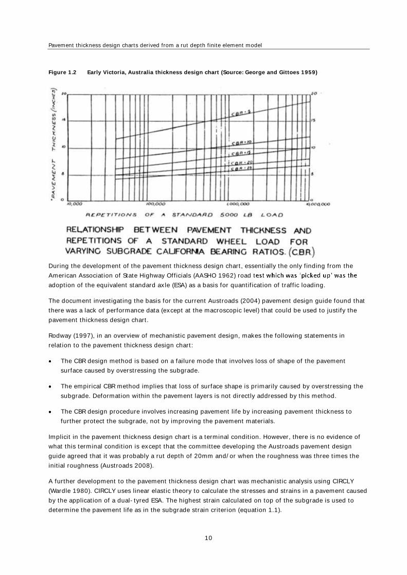
Figure 1.2 Early Victoria, Australia thickness design chart (Source: George and Gittoes 1959)
During the development of the pavement thickness design chart, essentially the only finding from the
American Association of State Highway Officials (AASHO 1962) road t
adoption of the equivalent standard axle (ESA) as a basis for quantification of traffic loading.
The document investigating the basis for the current Austroads (2004) pavement design guide found that
there was a lack of performance data (except at the macroscopic level) that could be used to justify the
pavement thickness design chart.
Rodway (1997), in an overview of mechanistic pavement design, makes the following statements in
relation to the pavement thickness design chart:
The CBR design method is based on a failure mode that involves loss of shape of the pavement
surface caused by overstressing the subgrade.
The empirical CBR method implies that loss of surface shape is primarily caused by overstressing the
subgrade. Deformation within the pavement layers is not directly addressed by this method.
The CBR design procedure involves increasing pavement life by increasing pavement thickness to
further protect the subgrade, not by improving the pavement materials.
Implicit in the pavement thickness design chart is a terminal condition. However, there is no evidence of
what this terminal condition is except that the committee developing the Austroads pavement design
guide agreed that it was probably a rut depth of 20mm and/or when the roughness was three times the
initial roughness (Austroads 2008).
A further development to the pavement thickness design chart was mechanistic analysis using CIRCLY
(Wardle 1980). CIRCLY uses linear elastic theory to calculate the stresses and strains in a pavement caused
by the application of a dual-tyred ESA. The highest strain calculated on top of the subgrade is used to
determine the pavement life as in the subgrade strain criterion (equation 1.1).

1 Introduction
11
(Equation 1.1)
where:
Nf [-] number of standard axle repetitions (SAR) to failure
[10-6 m/m] compressive elastic strain at the top of the subgrade produced by the
load (Austroads 2004).
The subgrade strain criterion was developed by computing the vertical compressive strain (using CIRCLY
and standard assumptions) on top of the subgrade for a range of subgrade CBRs and thicknesses and
plotting this with life (number of ESAs) from the pavement thickness design chart (figure 1.1). Hence,
whether CIRCLY or the design chart (figure 1.1) is used, the same life will be determined.
In summary, the current design procedure started with a CBR thickness design chart in California which at
best was developed from experience at the time of what seemed to work, rather than a specific scientific
experiment. The AASHTO road test only made a minor improvement by developing a method for
combining all traffic types into one ESA. Further, the introduction of mechanistic pavement design with the
use of CIRCLY has not improved the design procedure as it is aimed to achieve the same answer as the
design chart.
Implicit in the current pavement design procedure is that pavement life can increase exponentially by
simply increasing the depth of granular cover to the subgrade. This may be the case for roads with traffic
volumes most likely up to 2 million ESAs, which is the limit of observed pavement performance by roading
designers. This observation has been extrapolated to 10 and 100 million ESAs but never validated with
experiments. There is some anecdotal evidence in New Zealand from the Canterbury accelerated pavement
testing indoor facility (CAPTIF) and recent roads constructed on high traffic roads (eg Alpurt) that granular
pavements require rehabilitation before 10 million ESAs regardless of the granular pavement thickness. A
reason for this is that rutting occurs in the sub-base and basecourse materials and this has not been
considered in the current design procedure.
Research at CAPTIF has shown that at least 50% of rutting can occur in the unbound granular material
layers (Arnold et al 2001). Further, different aggregates complying to the same specification have clearly
shown differences in the amount of rutting occurring within the layer. Average results from 51 trenches in
the AASHTO road test were described as follows: a rut on the surface of the pavement was attributed to
changes in thickness of 32 percent, 14 percent, and 45 percent, respectively, in surfacing, base and
subbase, and to a rut in the embankment soil equal to 9 percent of the total (Benkelman 1962). Thus the
quality/rut resistant properties of the granular pavement layers can influence the pavement design. The
use of rut depth modelling in this research project was intended to determine the differences in pavement
life with different quality aggregates.
1.2 Observations at the Canterbury accelerated pavement testing indoor facility (CAPTIF)
Tests at CAPTIF studying the effects of changes in mass limits, used two different pavement depths and
three aggregate types on the same subgrade type (CBR=10). The two basecourse depths used were
200mm and 275mm and from figure 8.4 in the Austroads pavement design guide (1992 and 2004) this
represents pavement lives of 0.1 and 2 million ESAs respectively. However, the results from the CAPTIF
tests (Arnold et al 2005) predicted only minor differences in pavement life due to changes in pavement
79 300
Nf

Pavement thickness design charts derived from a rut depth finite element model
12
depth (table 1.1). This questions the applicability of the current Austroads pavement thickness design
chart and associated Austroads subgrade strain criterion (equation 1.1) currently used in design.
Table 1.1 Pavement life predicted for each segment in CAPTIF mass limits test (Arnold et al 2005)
Segment Material Depth
(mm)
Number ESAsa for
20mm rut depth
(Predicted from linear
extrapolation of data)
Life predicted
by Austroads
A Australian
AP20
275 3.5 million 2 million
B Australian
AP20
200 4.2 million 0.1 million
C TNZ M4
(AP40)
200 3.6 million 0.1 million
D TNZ M4
(AP40)
275 4.2 million 2 million
a ESA is equal to 8.2 tonnes on a dual-tyred single axle or 80kN.
1.3 Models to predict pavement rutting
The CAPTIF pavements detailed in table 1.1
Nottingham, England (Arnold 2004). This model utilised a relationship with stress and deformation
derived from repeated load triaxial tests (RLT) on the aggregates and subgrade used at CAPTIF. A finite
element model was used to compute stresses, which were inputted into the RLT deformation model to
calculate the surface rut depth. Predicted rut depths were close to those that actually occurred at CAPTIF
(table 1.1).
Werkmeister also developed a pavement model using relationships between resilient strain and permanent
strain found from RLT tests to predict rutting at CAPTIF and found a good match between measured and
predicted rutting (Werkmeister et al 2005).
Rut depth models (Arnold 2004; Werkmeister 2007) were used to derive pavement thickness design charts
for granular pavements. After validating the rut depth model against recent CAPTIF tests, a range of
pavements with different thicknesses and subgrade types was modelled to predict life (number of ESA
passes until a 10, 15, 20 and 25mm rut depth). Results of this analysis were amalgamated to produce a
granular pavement thickness design chart relating subgrade CBR, life (ESAs) and granular pavement
thickness in the same format as the Austroads design chart (figure 1.1). Production of the design chart
was repeated for poor, average and very good quality granular material as determined from the RLT test. It
should be noted that the poor, average and very good aggregates all comply with the relevant NZ
Transport Agency specifications and are only differentiated by the RLT test.
1.4 Other models to predict rutting
Over the years many researchers have begun to develop models for the prediction of permanent
strain/rutting in unbound materials. Many of these relationships have been derived from permanent strain
RLT tests. The aim of the models is to predict the magnitude of permanent strain from known loads and
stress conditions. There are many different relationships reviewed in this section with quite different

1 Introduction
13
trends in permanent strain development. The differences in relationships are likely to be a result of the
limited number of load cycles and different stress conditions tested in the RLT apparatus. It is likely that
more than one relationship is needed to fully describe the permanent strain behaviour of granular
material.
For convenience and comparison, the relationships proposed for permanent strain prediction have been
group in table 1.2 (after Lekarp 1997 except for those relationships from Theyse 2002). Details of the
Werkmeister and Arnold methods for predicting rutting are described in the next section.

Pavement thickness design charts derived from a rut depth finite element model
14
Table 1.2 Models proposed to predict permanent strain (after Lekarp 1997 except relationships from Theyse 2002)
Expression Eqn. Reference Parameters
b
rpNa
,1 1.1 Veverka (1979) p,1
*
,1 p
refpN
,1
pv ,
ps ,
N
i
r
pK
pG
q
p
0q
0p
*p
0p
L
= accumulated permanent strain after N load
repetitions
= additional permanent axial strain after first 100
cycles
= accumulated permanent axial strain after a
given number of cycles Nref
, Nref
> 100
= permanent volumetric strain for N > 100
= permanent shear strain for N > 100
= permanent strain for load cycle N
= permanent strain for the first load cycle
= resilient strain
= bulk modulus with respect to permanent
deformation
= shear modulus with respect to permanent
deformation
= deviator stress
= mean normal stress
N
pNK
pv
p
,
, N
qNG
ps
p
,3
2
2
DN
NAG
p ,
3
3
DN
NA
K
G
p
p
1.2
1.3
Jouve et al (1987)
bpNA
N1
,1
1.4
Khedr (1985)
Nbap
log,1
1.5
Barksdale (1972)
b
paN
,1 1.6 Sweere (1990)
bN
peacN 1
,1 1.7 Wolff and Visser (1994)
4
4*
,1
DN
NAp
1.8 Paute et al (1988)
B
p
NA
1001*
,1 1.9 Paute et al (1996)
ihNpN
1,1
1.10
Bonaquist and Witczak (1997)

1 Introduction
15
Expression Eqn. Reference Parameters
sin1
)sincos(2/1
3
3
,1CqR
aq
f
b
p
1.2 Barksdale (1972)
3
N
S
S95.0
= modified deviator stress= q32
= modified mean normal stress= p3
= stress parameter defined by intersection of the static failure line and the p-axis
= reference stress
= stress path length
= confining pressure
= number of load applications = static strength
= static strain at 95% of static strength
NSqb
Sqa
S
qSp
ln1
1ln
15.0
95.0,1 1.3
Lentz and Baladi (1981)
C
fnN
Rf
h
A1
A2-A4,
D2-D4
M
a, b, c,
d
A, B, t,
u
PD
a
1
SR
= apparent cohesion = angle of internal friction
= shape factor = ratio of measured strength to ultimate hyperbolic strength = repeated load hardening parameter, a function of stress to strength ratio = a material and stress-strain parameter given (function of stress ratio and resilient modulus)
= parameters which are functions of stress ratio q/p
= slope of the static failure line
= regression parameters (A is also the limit value for maximum permanent axial strain) = permanent deformation (mm)
= applied major principal stress
= shear stress ratio (a theoretical maximum value of 1 indicates the applied stress is at the limit of materials shear strength defined by C and )
3
,19.0
qp
1.4 Lashine et al (1971)
8.2
max
0
0
,fn
p
qLN
ps 1.5 Pappin (1979)
*
*
pp
qmb
pp
q
A 1.6 Paute et al (1996)
b
refp
p
qa
pL
N
max0
,1 1.7 Lekarp and Dawson (1998)
sr
a
B
pp
q
p
NAN
1
1001 1.8 Akou et al (1999)

Pavement thickness design charts derived from a rut depth finite element model
16
Expression Eqn. Reference Parameters
bb
a
cN
cNdNPD
1
1
1.9
RD
St
PS
= relative density (%) in relation to solid density
= degree of saturation (%)
= plastic strain (%)
bNeadNPD 1 1.10
utuetePD bNaN 1.11
SRPSStRDN 02.007.007.029.043.13log 1.12
245tan21
245tan 002
3
31
C
SR
a
1.13
Theyse (2002)

1 Introduction
17
1.5 Repeated load triaxial tests to obtain parameters for rut depth models
The RLT apparatus (figure 1.3) applies repetitive loading on cylindrical materials for a range of specified
stress conditions, the output is deformation (shortening of the cylindrical sample) versus number of load
cycles (usually 50,000) for a particular set of stress conditions. Multi-stage RLT tests are used to obtain
deformation curves for a range of stress conditions to develop models for predicting rutting (figure 1.4).
The method developed by Arnold (2004) for interpreting the RLT results involves relating stress to
permanent deformation found from the test. Similarly Werkmeister (2007) developed a model that relates
resilient strain to permanent deformation found from the RLT test.
Figure 1.3 Repeated load triaxial apparatus
Figure 1.4 Typical results from multi-stage permanent strain RLT test (note: A, B, C, D, E and F represent
different loading stresses for both cell pressure and vertical load)
A standard test for granular materials has been developed and detailed in NZTA T/15 Specification for
repeated load triaxial testing (RLT) of unbound and modified road base aggregates which gives stresses
suitable for testing granular materials. However, these stresses are not suitable for testing subgrade soils
0
0.2
0.4
0.6
0.8
1
0 50,000 100,000 150,000 200,000 250,000 300,000
Number of load cycles [-]
Perm
anent str
ain
[%
]
AB
CD
E
F

Pavement thickness design charts derived from a rut depth finite element model
18
which will fail by shear after the first load is applied. Arnold (2004) conducted RLT tests on the subgrade
at CAPTIF using stresses that were less than the shear strength of the soil. Another method for
determining appropriate stresses to test soils is to allow the first test to be sacrificial and then to conduct
a 30-stage test of 1000 cycles for each test. Each stage results in an increase in loading and the stage
when the soil fails represents the highest loading that can be applied. Ideally at least six full stages are
completed to provide enough data for the rut depth models. In this research project, many RLT tests were
conducted on subgrade soils of CBR 2, 8 and 10 as used at CAPTIF to determine the necessary parameters
for the rut depth model.

2 Rut depth prediction methods
19
2 Rut depth prediction methods
2.1 Arnold (2004) rut depth prediction method
2.1.1 Introduction
The first step in predicting rutting is to undertake multi-stage permanent strain RLT tests on the materials
in the pavement including the subgrade, subbase and basecourse. This allows relationships between
stress and permanent deformation to be determined for each material in the pavement. From the RLT
tests, a relationship between stress and resilient modulus is also determined for use in a finite element
programme to determine stresses and strains in the pavement at incremental depths. These stresses and
strains are imported into a spreadsheet where the rut depth is calculated at each depth increment using
the relationships to predict rutting found from RLT testing.
2.1.2 RLT tests
Using the RLT apparatus, Arnold (2004) studied the effect of different combinations of cyclic vertical and
horizontal stress levels on a range of granular materials. The granular materials chosen were those used in
full-scale pavement tests in Northern Ireland, UK and at CAPTIF. The subgrade silty clay soil used at
CAPTIF was also tested in the RLT apparatus.
The aim of the RLT tests was to determine the effect of stress condition on permanent strain. RLT
permanent strain tests are time consuming and many tests are needed to cover the full spectrum of
stresses expected within the pavement. To cover the full spectrum of these stresses Jouve and Guezouli
(1993) conducted a series of permanent strain tests at different combinations of cell pressure and cyclic
vertical load. Most of the stresses calculated by Jouve and Guezouli (1993) showed the mean principal
stress (p = ( + 2 )/3) varied from 50kPa to 300kPa and the deviatoric stress (q = (1 3
)) from 50kPa to
700kPa. These ranges of stresses were confirmed by the authors through pavement analysis using the
CIRCLY linear elastic program (Wardle 1980). Although at the base of the granular layers negative values
of p were calculated, as a granular material has limited tensile strength, negative values of mean principal
stress were discounted. The results of the static shear failure tests conducted on the materials plotted in
p q stress space were used as an approximate upper limit for testing stresses.
It is common to use a new specimen for each stress level. However, to reduce testing time, multi-stage
tests were devised and conducted. These tests involved applying a range of stress conditions on one
sample. After the application of 50,000 load cycles (if the sample had not failed) new stress conditions
were applied for another 50,000 cycles. These new stress conditions were always slightly more severe (ie
closer to the yield line) than the previous stress conditions.
Test stresses were chosen by keeping the maximum value of p constant while increasing q for each new
increasing stress level closer and occasionally above the static yield line. Three samples for each material
were tested at three different values of maximum mean principal stress p (75kPa, 150kPa and 250kPa).
This covered the full spectrum of stresses in p q stress space so as to allow later interpolation of
permanent strain behaviour in relation to stress level. A typical output and stress paths from a multi-stage
RLT test is shown in figure 2.1.

Pavement thickness design charts derived from a rut depth finite element model
20
Figure 2.1 Typical RLT permanent strain test result for NI Good UGM
2.1.3 Modelling permanent strain
Results from RLT tests showed a high dependence on stress level. Plots of maximum deviator stress, q
versus permanent strain rate for each multi-stage test analysed separately with mean principal stress, p
constant, resulted in exponential relationships that fitted well to the measured data (figure 2.1). This
prompted an investigation of an exponential model that could determine the secant permanent strain rate
from the two maximum values of q, p stress.
Utilising the rate of deformation seemed more appropriate for RLT multi-stage tests than using the
accumulated sum of the permanent strain for each part of the multi-stage test. Adding the sum of the
permanent strains of all the previous stages would likely over-estimate the amount of deformation, for
example by increasing the number of test stages conducted prior to that of the present stress level in
question, and would lead to a higher magnitude of permanent strain. Also on reviewing the RLT
permanent strain results during the first 20,000 load cycles, there was a bedding in phase until a more
stable/equilibrium type state was achieved. It had been argued that this equilibrium state was unaffected
by differences in sample preparation and previous tests in the multi-stage tests. Therefore, relationships
considering permanent strain rate were explored.
The scatter in results was reduced by using the secant rate of permanent strain between 25,000 and
50,000 load cycles in place of permanent strain magnitude when plotted against stress ratio (q/p). This
rate of permanent strain was calculated in percent per 1 million load cycles. These units have some
practical interpretation, as a value of 5% per million load cycles can be approximately related to 5mm of
deformation occurring for a 100mm layer after 1 million load applications.
0.0
0.5
1.0
1.5
2.0
2.5
3.0
0.0E+
00
5.0E+
04
1.0E+
05
1.5E+
05
2.0E+
05
2.5E+
05
3.0E+
05
Loads
Pe
rma
ne
nt S
tra
in (
%)
AB
C
D
E
F
Testing Stress (kPa)
A: q = 381; 3 = 116
B: q = 433; 3 = 99
C: q = 482; 3 = 82
D: q = 526; 3 = 67
E: q = 572; 3 = 50
F: q = 621; 3 = 33
(p = 250 kPa)

2 Rut depth prediction methods
21
Figure 2.2 Example plot showing how exponential functions fit measured data for individual multi-stage
tests
Regression analysis was undertaken on the RLT test data with stress invariants p and q against the
associated natural logarithm of the strain rate. Permanent strain rate is thus defined by equation 2.1:
p(rate or magn) = e(a)
e(bp)
e(cq)
– e(a)
e(bp)
(Equation 2.1)
= e(a) e(bp) (e(cq) 1)
where:
e = 2.718282
p(rate or magn) = secant permanent strain rate or can be just permanent strain magnitude
a, b & c = constants obtained by regression analysis fitted to the measured RLT data
p = mean principal stress (MPa)
q = mean principal stress difference (MPa).
To determine the total permanent strain for any given number of load cycles and stress condition, the
permanent strain data in four zones was observed. In the New Zealand accelerated pavement tests (Arnold
2004) the permanent strain rates changed during the life of the pavements, different values being
associated with the early, mid-, late- and long-term periods of trafficking. Similarly RLT permanent strain
tests showed changing permanent strain rates during their loading. After studying RLT and accelerated
pavement test results, a power law equation of the form, y=axc was fitted to each 50,000 RLT load cycle
stage (figure 2.3) to extend the permanent strain data to 500k or 1 million load cycles (note the analysis
for determining pavement life uses both methods for comparison). To limit the number of times equation
2.1 was used to fit the RLT data, it was decided to break the RLT permanent strain data into the following
four zones of different behaviour for use in calculating permanent strain at any given number of load
applications (N) (figure 2.3):
1 Early behaviour (compaction important): 0 25,000 load applications. The magnitude of permanent
strain at 25,000 load applications, being the incremental amount p(25,000), was used for the reasons
outlined above. Keeping the magnitude of permanent strain separate at 25,000 was useful when
predicting rut depth in terms of identifying where the errors occurred.
0.0
0.5
1.0
1.5
2.0
0.00 0.20 0.40 0.60 0.80 1.00
Principal Stress Difference, q (MPa)
Perm
an
en
t str
ain
rate
(%
/1M
)
(25k
to
100k
)
0.075
0.150
0.250
0.075
0.150
0.250
CAPTIF 3
R2 = 0.92
Mean Principal Stress, p (MPa)

Pavement thickness design charts derived from a rut depth finite element model
22
2 Mid-term behaviour: 25,000 50,000 load applications. The secant permanent strain rate between
25,000 and 50,000 load applications was used.
3 Mid-term behaviour: 50,000 100,000 load applications. The secant permanent strain rate between
50,000 and 100,000 load applications was used.
4 Late behaviour: 100,000 500,000 load applications. The secant permanent strain rate between
100,000 and 500,000 load applications was used. This is extended to represent the long-term
behaviour as a conservative approach to predicting the rut depth.
This assumed that the permanent strain rate remained constant after 1 million load applications. The
approach was appropriate as the aim was to calculate rut depth for pavements with thin surfacings where at
CAPTIF Arnold (2004) found the rate of rutting was linear. Further, assuming the permanent strain rate did
not decrease after 1 million load applications was a conservative estimate compared with the assumption of
permanent strain rate continually decreasing with increasing load cycles (ie a power model, y= axb).
Hence, four versions (four sets of constants) of equation 2.1 were determined and used for describing the
permanent strain behaviour at any given number of loadings.
Figure 2.3 Methods of extrapolation of RLT data and rut depth prediction
The RLT multi-stage permanent strain test results for six granular and one subgrade material were
analysed by relating the permanent strain rate with the stress level for each stage. Microsoft Excel© Solver
was used to determine the equation constants a and b by minimising the mean error which was the
difference in measured and calculated strain rates. For the CAPTIF 3 granular material, the model fitted the
data well with a R2 value of 0.92 (figure 2.2). A similar good fit to the model (equation 2.1) was found for
the other five granular and one subgrade materials tested. Mean errors were less than 1%/1 million which,
when applied to rut prediction, gave an equivalent error of 1mm per 100mm thickness for every 1 million
wheel passes. Overall the model (equation 2.1) showed the correct trends in material behaviour as there
was an increasing permanent strain rate with increasing deviatoric stress (q) while a higher load could be
sustained with higher confining stress.
0
0.5
1
1.5
2
2.5
3
3.5
4
4.5
5
0.0E+00 1.0E+06 2.0E+06 3.0E+06 4.0E+06 5.0E+06 6.0E+06 7.0E+06 8.0E+06 9.0E+06 1.0E+07
Number of Load Cycles (N)
Cu
mu
lati
ve P
erm
an
en
t S
train
(%
)
Power law extrapolation
Extrapolation - power law then linear
from 0.5 Million ESA
(using slope from 0.1 to 0.5 MESA)
RLT Data to 50k
Extrapolation - power law then linear
from 1 Million ESA
(using slope from 0.5 to 1.0 MESA)

2 Rut depth prediction methods
23
2.1.4 Calculating pavement rut depth
To predict the surface rut depth of a granular pavement from equation 2.1 required a series of steps.
There were assumptions required in each step which significantly affected the magnitude of calculated rut
depth. Steps and associated errors and assumptions are summarised below. The first five steps related to
the interpretation of RLT permanent strain tests as already described in section 2.1.3 above. The final
three steps involved pavement stress analysis, calculations and validation required to predict the surface
rut depth of a pavement.
2.1.4.1 Pavement stress analysis
Equation 2.1 is a model where for any number of load applications and stress conditions the permanent
strain can be calculated. Stress is therefore computed within the pavement under a wheel load for use in
equation 2.1 to calculate permanent strain. It is recognised from literature and RLT tests that the stiffness
of granular and subgrade materials are highly non-linear. A non-linear finite element (FE) model, DEFPAV
(Snaith et al 1980) was originally used to compute stresses within the pavement (Arnold 2004). Rubicon is
now used as a more versatile finite element program to calculate stresses and strains in the pavement
using non-linear relationships between stress and resilient modulus for each material. Further, the small
residual confining stresses considered to occur during compaction of the pavement layers were assumed
to be nil in the analysis.
From the pavement stress analysis, the mean principal stress (p) and deviatoric stress (q) under the centre
of the load were calculated for input into a spreadsheet along with depth for the calculation of rut depth.
The calculated stresses had a direct influence on the magnitude of permanent strain calculated and
resulting rut depth. Thus any errors in the calculation of stress would result in errors in the prediction of
rut depth. Some errors in the calculation of stress from Rubicon and DEFPAV were a result of not
considering the tensile stress limits of granular materials and the assumption of a single circular load of
uniform stress approximating dual tyres, which did not have a uniform contact stress (de Beer et al 2002).
2.1.4.2 Surface rut depth calculation
The relationships derived from the RLT permanent strain tests were applied to the computed stresses in
the FE analysis. Permanent strain calculated at each point under the centre of the load was multiplied by
the associated depth increment and summed to obtain the surface rut depth.
2.1.4.3 Validation
The calculated surface rut depth with the number of wheel load applications was compared with actual rut
depth measurements from accelerated pavement tests in New Zealand (CAPTIF) and the Northern Ireland
(NI) field trial. This comparison determined the amount of rut depth adjustment required at 25,000 cycles
while the long-term rate of rut depth progression and, in part, the initial rut depth at 25,000 cycles was
governed by the magnitude of horizontal residual stress added. An iterative process was required to
determine the initial rut depth adjustment and the amount of horizontal residual stress to add, in order
that the calculated surface rut depth matched the measured values.
The result of this validation process was detailed fully in Arnold (2004). Overall the predictions of rut
depth were good, particularly the trends in rut depth progression with increasing loading cycles (ie this
relationship was sensibly the same for actual and predicted measurements in 11 out of 17 analyses).
Adjustment of up to a few millimetres to the predicted rut depth at 25,000 cycles was generally all that
was needed to obtain an accurate prediction of rut depth. For the six tests with poor predictions, three of
these could be accurately predicted by applying a small residual stress of 17kPa to the stresses calculated

Pavement thickness design charts derived from a rut depth finite element model
24
in the pavement analysis. The other three poor results were due to an asphalt layer of 100mm and a
moisture sensitive aggregate where the RLT test was at a higher moisture content than what actually
occurred in the test pavement. The predictions were as expected in terms of accurately predicting the rate
or rutting but inaccurately predicting the initial rutting due to secondary consolidation. This is because the
actual magnitude for the first 25,000 load applications from the RLT test was difficult to estimate, as it
was unknown whether the value was the cumulative or incremental value of permanent strain from the
multi-stage RLT test (figure 2.1 1). The method adopted was to take the incremental value of permanent
strain at 25,000 cycles, which was considered to be a low estimate. This was the case for pavement test
sections 3, 3a and 3b which all used the CAPTIF 3 granular material and for test sections 4, 5 and 6 where
an additional amount of rutting was added to coincide with the measured values in the pavement test. The
opposite occurred for the test sections 1, 1a and 1b which all used the CAPTIF 1 material where the
predicted rutting was higher than the measured rutting.
Further validation of the Arnold method was undertaken when analysing recent CAPTIF tests that used a
different subgrade material. These are described in chapter 4 of this report.
2.2 Description of Werkmeister model
This section presents an approach to predict the plastic deformation of the basecourse/subgrade in
pavements using the elastic strains. The investigation was based on RLT and CAPTIF test results and used
the axial elastic strain to predict the axial plastic strain rate per load cycle. The relationship developed
using laboratory and field results was applied to the axial elastic strains calculated and integrated over the
depth of the basecourse layer and the number of load cycles in the CAPTIF tests to determine the plastic
deformation (rut depth) occurring in the basecourse. The advantage of this simplified method to predict
the rut depth of the basecourse was that only elastic FE calculation results (elastic strain distribution in the
wheel path) were required. The elastic FE calculation process was less complicated and time consuming
than plastic FE calculations.
A similar approach was suggested by Theyse (2004) for the pavement subgrade from heavy vehicle
simulator (HVS) results. However, the plastic subgrade deformation was not taken into account in this
investigation.
2.2.1 Modelling the steady state phase using RLT test results
The raw RLT test data was obtained from Arnold (2004) and analysed in terms of elastic axial strain (el)
and the plastic strain rate ( p /N). Because the initial part of the plastic deformation curve is often
influenced by the technique used in preparing the sample, it was decided to extrapolate the plastic
deformation curve and focus on the steady state response of the sample (load cycles 100,000 to 500,000,
see figure 2.4).

2 Rut depth prediction methods
25
Figure 2.4 Determination of plastic strain rate value
The elastic strain value (el) was averaged over the same interval (load cycles 100,000 to 500,000) to give
an average value of el.
Using the RLT test results, the following relationship (equation 2.2) between the elastic strain (el
) and
plastic strain rate ( p ) can be determined as long as the shear stresses within the basecourse are
sufficiently small and the material behaviour corresponds to either a continually reducing plastic strain
rate with increasing load cycles or a constant plastic strain rate. Excluded from the fit were the tests that
failed prior to 50,000 load cycles, which was usually the highest stress level in each multi-stage (MS) test.
Results where failure occurs do not follow the same trend as the other results due to significantly larger
deformations/shear failure (range C behaviour) and this mechanism of accumulation of plastic strain is
different from the other test results.
F
elp E (Equation 2.2)
where:
p [10-3/cycle] major principal plastic strain rate
el [10-3] major principal elastic strain
E, F [-] material parameter.
The parameters E and F are mainly dependent on the material, moisture content and degree of compaction
and were determined for the CAPTIF 1, Todd clay and Waikari clay materials. Figures 2.5, 2.6 and 2.7 show
the relationship between axial elastic strain and axial plastic strain rate per load cycle on a (el
) vs ( p )
plot.
0
100
200
300
400
500
600
700
800
0 100000 200000 300000 400000 500000
Number of load cycles [-]
Perm
an
en
t str
ain
[m
/m]
Stage A calculated

Pavement thickness design charts derived from a rut depth finite element model
26
Figure 2.5 Axial elastic strain versus plastic strain rate for CAPTIF 1 material, RLT test results
Figure 2.6 Axial elastic strain versus plastic strain rate for Todd Clay material, RLT test results
Figure 2.7 Axial elastic strain versus plastic strain rate for Waikari Clay material, RLT test results
y = 4E-06x 1.91
R 2 = 0.95
0.00E+00
5.00E-06
1.00E-05
1.50E-05
2.00E-05
2.50E-05
3.00E-05
3.50E-05
4.00E-05
0.00E+00 5.00E-01 1.00E+00 1.50E+00 2.00E+00 2.50E+00 3.00E+00 3.50E+00
Elastic strains [10 -3 ]
Pla
sti
c s
train
rate
[10
]
-6
y = 2E-06x 0.6998
R 2 = 0.93
0.00E+00
5.00E-07
1.00E-06
1.50E-06
2.00E-06
2.50E-06
3.00E-06
3.50E-06
4.00E-06
4.50E-06
0.000 0.500 1.000 1.500 2.000 2.500 3.000
Elastic strains [10 -3 ]
Pla
stic s
train
rate
[10
-6]
y = 5E-06x 2.87
R 2 = 0.92
0.0E+00
2.0E-06
4.0E-06
6.0E-06
8.0E-06
1.0E-05
1.2E-05
0.00 0.50 1.00 1.50 2.00
Elastic strain rate per load cycle [10 -3 /load cycle ]

2 Rut depth prediction methods
27
In most cases, CAPTIF elastic data consists of direct measurements of the elastic strains between the two
wheels using mu strain coils. The program ReFEM (Oeser 2004) was used to determine the distribution of
axial elastic strains directly underneath the wheels for the load applied in the CAPTIF tests. The averages
of these axial elastic basecourse strain values were taken for the determination of the CAPTIF elastic strain
values (field results).
The CAPTIF test results showed a similar dependency between the elastic strain and the plastic strain rate
to the results of laboratory tests. By comparing the elastic/plastic relationship from laboratory tests and
the elastic/plastic relationship from field tests, a good correlation was observed. In addition, the results
proved that the RLT test was a suitable testing method to investigate the stress-strain behaviour of
basecourse materials used in pavements.
The model developed (equation 2.2) was linear and therefore suited only to cases where plastic strain was
expected to be a shakedown range B response. Although, for low-stress levels the model would calculate
a low value of plastic strain and therefore it might suffice for expected range A responses also.
Figure 2.8 illustrates the elastic strain distribution in the basecourse layer under a 40kN and 50kN wheel
load using the FE calculation results. The plastic strain values during the steady state phase were
determined for the basecourse using equation 2.2 (PR3-0404 test, CAPTIF 1 material). The analysis shows
that the most critical (maximum) vertical elastic and plastic strains occurred at the first third of the
basecourse layer for the pavements investigated.
In addition, the calculated plastic strain values using equation 2.2 were compared with the measured
plastic strain values at CAPTIF. The calculated plastic strain values ( p ) at different depths of the
basecourse were calculated to give an average value of ( p
). A good agreement between the calculated
plastic strain rates and the measured plastic basecourse strain rate values at CAPTIF could be observed.
For most of the pavements, range B behaviour was measured. However, one station of the PR3-0610 test
showed range A behaviour.
Figure 2.8 Measured plastic strain rate versus calculated plastic strain rate, PR3-0610 test, inner and outer
wheel path

Pavement thickness design charts derived from a rut depth finite element model
28
2.2.2 Modelling of post-construction compaction using CAPTIF test results
CAPTIF test data was used to investigate the post-construction compaction and to determine a
relationship between the axial plastic strain rate during post-construction compaction and during the
steady state phase.
CAPTIF test results showed that the number of load cycles until completion of post-construction
compaction was dependent on the elastic strains. Using CAPTIF test results (PR3-0404 and PR3-0610
tests) a relationship between the axial elastic strains (el) and the number of load cycles (Npc) for the
completion of post-construction compaction could be determined (equation 2.3 and figure 2.9).
8232.071.211 elpcN (Equation 2.3)
where:
pc [-] = number of load cycles for completion of post-construction compaction.
el [10-6] = axial elastic strain.
Figure 2.9 Axial elastic strain versus number of load cycles until post-construction compaction is completed
The following exponential relationship (equation 2.4) between the plastic strain rate during the steady
state phase ( p ) and the plastic strain rate during post-construction compaction ( p
pc) was found using
CAPTIF test results (PR3-0404 and PR3-0610 test).
6869.0
0042.0 pR (Equation 2.4)
where:
p [10-3/cycle] = plastic strain rate per load cycle during steady state phase
R [-] = ratio between plastic strain rate (post-construction compaction) and plastic
strain rate (steady state).
2 Rut depth prediction methods
29
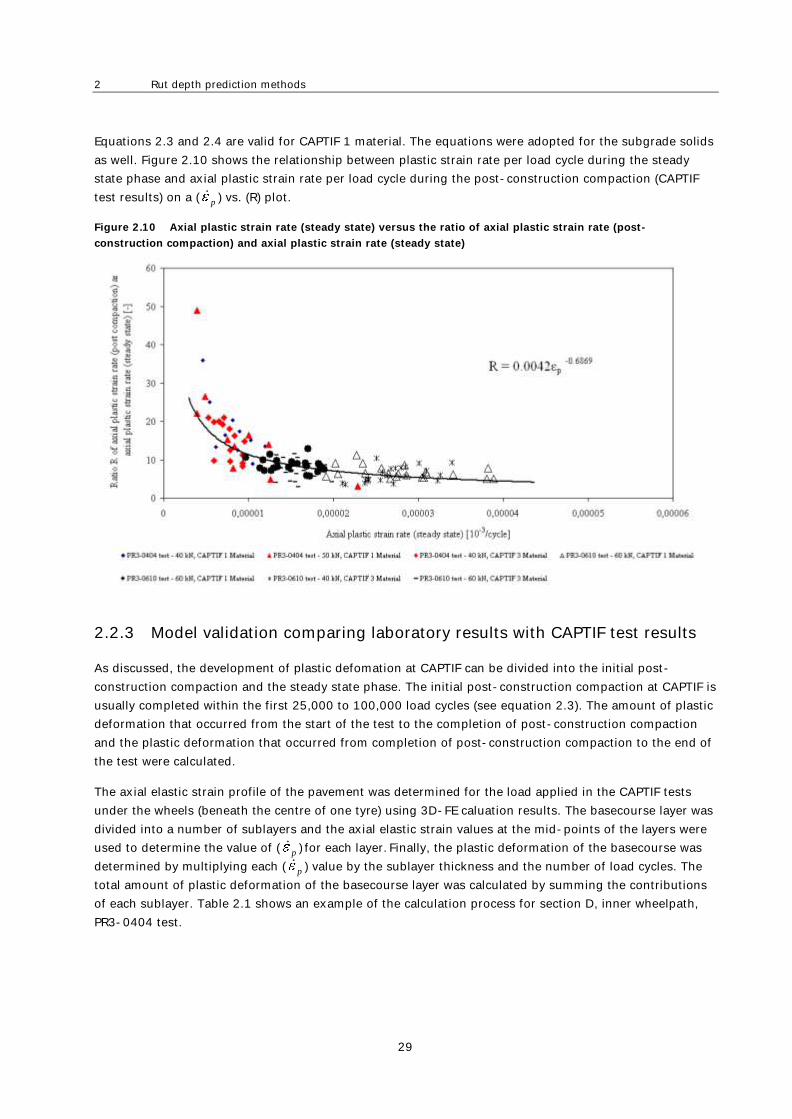
Equations 2.3 and 2.4 are valid for CAPTIF 1 material. The equations were adopted for the subgrade solids
as well. Figure 2.10 shows the relationship between plastic strain rate per load cycle during the steady
state phase and axial plastic strain rate per load cycle during the post-construction compaction (CAPTIF
test results) on a ( p ) vs. (R) plot.
Figure 2.10 Axial plastic strain rate (steady state) versus the ratio of axial plastic strain rate (post-
construction compaction) and axial plastic strain rate (steady state)
2.2.3 Model validation comparing laboratory results with CAPTIF test results
As discussed, the development of plastic defomation at CAPTIF can be divided into the initial post-
construction compaction and the steady state phase. The initial post-construction compaction at CAPTIF is
usually completed within the first 25,000 to 100,000 load cycles (see equation 2.3). The amount of plastic
deformation that occurred from the start of the test to the completion of post-construction compaction
and the plastic deformation that occurred from completion of post-construction compaction to the end of
the test were calculated.
The axial elastic strain profile of the pavement was determined for the load applied in the CAPTIF tests
under the wheels (beneath the centre of one tyre) using 3D-FE caluation results. The basecourse layer was
divided into a number of sublayers and the axial elastic strain values at the mid-points of the layers were
used to determine the value of ( p )
for each layer.
Finally, the plastic deformation of the basecourse was
determined by multiplying each ( p ) value by the sublayer thickness and the number of load cycles. The
total amount of plastic deformation of the basecourse layer was calculated by summing the contributions
of each sublayer. Table 2.1 shows an example of the calculation process for section D, inner wheelpath,
PR3-0404 test.

Pavement thickness design charts derived from a rut depth finite element model
30
Table 2.1 Plastic deformation calculation for section D, PR3-0610 test (275mm BC, 40 kN load, subgrade
stiffness 50 MPa, CAPTIF 1 material)
Depth to
midheight
of the
sublayer
Sublayer
thickness
Elastic
strains
Plastic
strain
rate
steady
state
Plastic
deformation
steady state
Load cycles
post-
construction
compaction
Plastic
strain rate
post-
construction
compaction
Plastic
deformation
post-
construction
compaction
[mm] [mm] [10-3] [10-
3/cycle]
[mm] [-] [10-3/cycle] [mm]
25 34 1.364 1.35E-05 0.43 80,597 1.26E-04 0.35
94 69 1.575 1.97E-05 1.23 90,728 1.41E-04 0.88
163 69 1.221 1.01E-05 0.64 73,574 1.15E-04 0.58
231 69 0.981 5.71E-06 0.37 61,445 9.58E-05 0.40
325 34 0.971 5.56E-06 0.18 60,928 9.50E-05 0.20
Plastic basecourse deformation [mm] 2.85 2.41
In addition, the plastic basecourse deformation at CAPTIF was determined using the measured vertical
surface deformation/rutting (VSD) values. VSD values of both tyres were averaged to eliminate any
imbalance in plastic deformation between the two paths. Based on the results of the trench profiles the
plastic surface deformation values obtained were reduced to remove the plastic deformation that occurred
in the subgrade. The plastic deformation values for the different test sections are given in table 2.2. It can
be seen that the plastic deformation values for the post-construction compaction are relatively high
compared with the plastic deformation values during the steady state period.
Table 2.2 Comparison between calculated and measured plastic deformations beneath the tyre
Total Basecourse
CAPTIF Test Basecourse Basecourse Loading Measured Calculated Measured Calculated
Section Material [mm] [kN] [mm] [mm] [mm] [mm]
PR3-0805 E CAPTIF 1 300 40 5.0 6.81 3.7 4.55
PR3-0805 E CAPTIF 1 300 50 7.6 9.46 5.7 6.7
PR3-0610 C CAPTIF 1 200 40 6.5 6.16 4.9 4.2
PR3-0610 C CAPTIF 1 200 60 11.1 14.87 8.3 10.6
PR3-0404 A CAPTIF 1 275 40 6.0 6.44 3.6 4.4
PR3-0404 A CAPTIF 1 275 50 11.4 9.62 7.4 6.5
Figure 2.11 shows the number of load cycles versus the axial plastic deformation (in the wheel path) using
equations 2.2, 2.3 and 2.4.

2 Rut depth prediction methods
31
Figure 2.11 Axial plastic basecourse deformation versus N (data and model), PR3-0404 test, CAPTIF 1 material
2.2.4 Discussion
The results of the investigations showed a good agreement between the measured and calculated results.
However, an exact agreement between the real performance and the modelling results can never be
achieved because so many factors influence the deformation performance of the pavements. This is clearly
shown by the relatively high variation of the rut depth values measured at CAPTIF for the same pavement
structure within one section.
Furthermore the real pavement contact pressure distribution was not taken into account in the calculation
process. The accuracy of the models depends on the accurate portrayal of tyre/road contact stress
distributions. In a research project funded by the NZTA (Douglas 2009), an apparatus to measure
tyre/road surface contact stress distributions in all three coordinate directions was fabricated and
calibrated. A wide range of full-scale trafficking tests was carried out on the apparatus at CAPTIF and the
contact stress distributions were measured. The distributions were then input to numerical models of
uniformly distributed vertical pressure only, within the contact patch.
The research showed that due to the different tyre contact pressure modelling there were differences in
response, but they were often not large. Vertical stresses on top of the subgrade were 3% to 8% greater
when the non-uniform contact stresses were used. For dual tyres, the differences were greater at 12% to
27%, but the larger differences may well have been due to the unequal loading of the two tyres in the dual
set. These differences in response, though not particularly great, especially if some credit is given to the
unequal tyre loads in the dual tyre configurations, were enough however to affect the long-term pavement
performance significantly. The rut depths predicted using the non-uniform contact stresses were a little
over a quarter greater than those predicted using the conventional uniform pressure. However, it is felt
that there was enough evidence in the experimental results to conclude that there were small though
measurable differences in pavement response when modelled using non-uniform contact stresses, and
0
2
4
6
8
10
12
14
0 100 200 300 400 500 600 700 800 900 1000
Number of load cycles (x 1000) [-]
Ax
ial
pla
stic
to
tal
def
orm
atio
n [
mm
] .
CAPTIF 1 Material (40 kN)
Model
(40 kN)
CAPTIF PR3-0610 Test - Section C (Station 24 - 33)
Dual Tire Load 40 kN

Pavement thickness design charts derived from a rut depth finite element model
32
that these differences in pavement response gave rise to substantial differences in predicted pavement
performance (Douglas 2009).

3 Repeated load triaxial testing
33
3 Repeated load triaxial testing
3.1 Introduction
This section provides a summary of the results of RLT testing of subgrade soils used at CAPTIF. RLT tests
apply repetitive loading to cylindrical soil or aggregate specimens at user-defined vertical and confining
stresses. The aim is to replicate in some way the loadings expected to occur on the material when used in
a pavement. Information from the tests, such as rate of permanent deformation at a range of different
stress conditions, can be used in pavement models to calculate the amount of rutting expected to occur.
Rutting in all the pavement layers and subgrade soils are added together to compute the rut depth at the
surface and determine the number of wheel loads required to reach a defined end of life rut depth (eg
15mm or 25mm). Two different approaches of pavement modelling and rut depth prediction were used in
this research project: one was stress based (the Arnold 2004 method) and the other a strain-based
approach (the Werkmeister method). After validation of the assumptions and criteria used in each model
against CAPTIF results, the models were used to predict rutting for a range of pavement cross sections.
3.2 RLT test results for basecourse and sub-base aggregates
The first year of this research project involved getting the necessary laboratory data required for pavement
modelling and validation with CAPTIF data. RLT data is required for all the materials that make up the
different layers of the pavement: basecourse, sub-base and subgrade. RLT data from basecourses are
readily available from the many tests already conducted commercially and for research. Sub-base
aggregates are being tested in a related NZTA research project, Development of a basecourse/subbase
design criterion which is being carried out by the authors of this report. Out of the database of RLT tests
a poor, average and very good basecourse and sub-base were selected for rut depth modelling in this
project. All aggregates selected complied with NZTA specifications and they were only classified as poor,
average and very good depending on their performance in the RLT test (ie lower permanent deformation
was considered the best performance). In selecting aggregates, outliers were not considered (ie those
aggregates that behaved significantly different from the norm). Figure 3.1 shows the results of rut depth
prediction of RLT tests on a large number of basecourse aggregates from the NZTA research project,
Development of a basecourse/subbase design criterion . The poor basecourse confirmed to the lower
boundary in figure 3.1, while the average was the medium boundary and the very good was the upper
boundary.

Pavement thickness design charts derived from a rut depth finite element model
34
Figure 3.1 Results of basecourse RLT tests
A similar method to selecting sub-base aggregates was also used; however, on a significantly smaller
subset of RLT tests as found in the related NZTA research project, Development of a basecourse/subbase
design criterion .
3.3 RLT test results for subgrade soils
The initial subgrade soils chosen for testing were the Waikari Silty Clay and the Todd Clay as used in the
CAPTIF pavement tests. Different moisture contents and densities were tested both in the RLT test and
laboratory CBR.
RLT testing on subgrade soils was found to be problematic because for each type of soil, moisture content
and density causes large variation in strength. The strength of the soil governs the stress levels at which
each of the 50,000 load stages are set. The aim is to choose at least six stress stages (as this takes 24
hours to test) where the sample survives sufficiently to provide the Werkmeister and Arnold models with
enough data to relate deformation to stress and strain.
Initial RLT testing proved worthless for its data use but useful in helping to establish a suitable RLT test
for two reasons:
1 The six stress levels guessed were either too high or too low.
2 In the testing regime for each of the stress stages, the change in confining stress caused a slow
response of the soil to expand or contract in all directions.
1.00E+00
1.00E+01
1.00E+02
1.00E+03
1.00E+04
1.00E+05
1.00E+06
1.00E+07
1.00E+08
1.00E+09
1.00E+10
1.00E+11
1.00E+12
10 100 1000 10000
Resilient Strain
Life
(N
, E
SA
s)
Upper
Middle
Lower

3 Repeated load triaxial testing
35
Changing the confining stress for a RLT soil test had a negative effect on vertical deformation as, in some
cases, the sample expanded with increasing number of load cycles as a result of the new reduced
confining stress.
All RLT tests on soils were repeated and now the standard process is to conduct three RLT tests per soil
type, density and moisture. Each of the three RLT tests is a 6- to 8-stage test at one particular confining
stress and between each stage only the vertical load changes. To determine the most appropriate vertical
stresses in each stage, a 24-stage test was conducted first at 1000 load cycles, which was completed in
two hours. Results of this preliminary test determined the maximum vertical load that the soil could
support, which in turn became the upper limit for setting the stress levels for the 50,000 6- to 8-stage
test. This extensive testing yields at least 18 data points relating permanent strain rate to either stress or
strain.
A summary of RLT tests conducted on subgrades is detailed in table 3.1 with full results in appendix A.
Table 3.1 RLT tests on subgrade soils conducted
RLT # PS0026 # Soil MC DD Lab CBR Comments
1, 2, 3 Waikari Silty Clay 11.9 1.72 25 Not used - confining pressure
changes caused expansion and
too strong 7 Todd Clay 19.4 1.60 17
8 Todd Clay 24.2 1.58 8
10, 11, 12, 13 Todd Clay 30.0 1.43 2.0 Used
21, 22, 33 Fine Pumice 11.7 1.06 25 May use for comparison
40,41 Drury Quarry
Subgrade 50.5 1.09 6 May use for comparison
50, 51, 52 Todd Clay 21.2 1.51 ? Too dry and thus too strong cf
in situ at CAPTIF - not used
53, 54, 55 Todd Clay 23.7 1.56 8 Used
56, 57, 58 Todd Clay 26.5 1.49 5 Not used as not the same as at
CAPTIF
73, 74, 75 Waikari Silty Clay 12.0 1.85 10 Used

Pavement thickness design charts derived from a rut depth finite element model
36
4 Rut depth prediction CAPTIF pavements validation Arnold method
The main dataset used to validate the rut depth prediction models was from the NZTA research project
using CAPTIF entitled, Fatigue design criteria for low noise surfaces on New Zealand roads (Alabaster and
Fussell 2006). This project used the Todd Clay at two different moisture contents (ie 2% and 8% CBR) in
unbound granular pavements with OGPA surfacings. Both the basecourse aggregate and subgrade soils
were tested in the RLT apparatus to obtain the parameters required, first for the Rubicon non-linear finite
element model and then for the model relating stress to permanent deformation to calculate the rutting.
Two predictions of rutting were undertaken, the first assuming a linear increase in rutting 1 million ESAs
and the second a linear relationship assumed from 0.5 million ESAs. Results of these rutting predictions
are shown in figures 4.1 and 4.2 where both methods result in rut depths very close to those actually
measured. The linear extrapolation from 0.5 million ESAs results is shown, however, to be more
appropriate (figure 4.2) and is therefore the method used to determine rutting for other pavements. No
initial adjustments to the rutting predictions were needed to predict the rutting for the Todd CBR 8%
sections. However, as discussed below, a minor reduction of 2mm in the predicted rutting was required to
predict rutting in the Todd Clay CBR 2% sections.
Figure 4.1 Rut depth prediction assuming linear extrapolation from 1 MESA for the CAPTIF section using Todd
Clay with CBR 8%
0
5
10
15
0 0.5 1 1.5 2N (Million ESAs)
Ru
t D
ep
th (
mm
)
Actual - Average Actual - 10th %ile Basecourse - Predicted
Todd - Predicted Waik - Predicted Total - Predicted
Actual - 90th %ile
Predicted Rut Depths - linear extrapolation from 1.0MESA
307-Stage 1 - Section E - 40kN - Todd CBR 8%

4 Rut depth prediction CAPTIF pavements validation Arnold method
37
Figure 4.2 Rut depth prediction assuming linear extrapolation from 0.5 MESA for the CAPTIF section using
Todd Clay with CBR 8%
As discussed, predicting the rutting for the CAPTIF Todd Clay CBR 2% section required a subtraction of
2mm to the predictions (figures 4.3 and 4.4). This 2mm subtraction is considered minor and at least it
shows the predictions of rutting were not underestimating the rut depth. Therefore, to predict rutting for
other pavements with a CBR of 2% it was decided not to subtract 2mm from the predicted rut depths. This
is because the aim of this project was to develop new pavement thickness design charts for adoption by
the NZTA and hence the need to take a conservative approach. Should the need arise in the future, the
2mm could be deducted from the predicted rut depths.
Figure 4.3 Rut depth prediction assuming linear extrapolation from 0.5 MESA for the CAPTIF section using
Todd Clay with CBR 2% with no adjustment
0
5
10
15
0 0.2 0.4 0.6 0.8 1 1.2 1.4 1.6 1.8 2
N (Million ESAs)
Ru
t D
ep
th (
mm
)
Basecourse - Predicted Todd - Predicted CAPTIF VSD 90th %ile
Waik - Predicted Total - Predicted
Predicted Rut Depths no Adjustment
0
5
10
15
0 0.5 1 1.5 2
N (Million ESAs)
Ru
t D
ep
th (
mm
)
Basecourse - Predicted Actual - Average Waik - Predicted
Todd - Predicted Actual - 10th %ile Total - Predicted
Actual - 90th %ile
Predicted Rut Depths - linear extrapolation from 0.5MESA
307-Stage 1 - Section E - 40kN - Todd CBR 8%

Pavement thickness design charts derived from a rut depth finite element model
38
Results from the rut depth predictions of the CAPTIF pavements validated the rut depth prediction model
used by Arnold. The model was then used to calculate rutting for many other pavement depths in order to
develop pavement design charts for granular pavements and compare predictions of life with figure 8.4 in
the Austroads (2004) pavement design guide.
Figure 4.4 Rut depth prediction assuming linear extrapolation from 0.5 MESA for the CAPTIF section using
Todd Clay with CBR 2% with 2mm subtracted from predicted rut depths
0
5
10
15
0 0.5 1 1.5 2
N (Million ESAs)
Ru
t D
ep
th (
mm
)
Asphalt Basecourse - Predicted Todd - Predicted
CAPTIF VSD 90th %ile Waik - Predicted Total - Predicted
Predicted Rut Depths less 2mm
5 Rut depth prediction other methods Arnold method
39
5 Rut depth prediction other pavements Arnold method
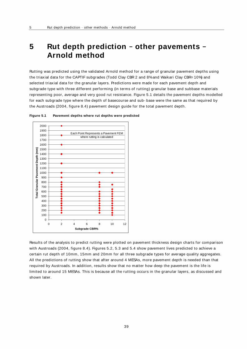
Rutting was predicted using the validated Arnold method for a range of granular pavement depths using
the triaxial data for the CAPTIF subgrades (Todd Clay CBR 2 and 8% and Waikari Clay CBR=10%) and
selected triaxial data for the granular layers. Predictions were made for each pavement depth and
subgrade type with three different performing (in terms of rutting) granular base and subbase materials
representing poor, average and very good rut resistance. Figure 5.1 details the pavement depths modelled
for each subgrade type where the depth of basecourse and sub-base were the same as that required by
the Austroads (2004, figure 8.4) pavement design guide for the total pavement depth.
Figure 5.1 Pavement depths where rut depths were predicted
Results of the analysis to predict rutting were plotted on pavement thickness design charts for comparison
with Austroads (2004, figure 8.4). Figures 5.2, 5.3 and 5.4 show pavement lives predicted to achieve a
certain rut depth of 10mm, 15mm and 20mm for all three subgrade types for average quality aggregates.
All the predictions of rutting show that after around 4 MESAs, more pavement depth is needed than that
required by Austroads. In addition, results show that no matter how deep the pavement is the life is
limited to around 15 MESAs. This is because all the rutting occurs in the granular layers, as discussed and
shown later.
0
100
200
300
400
500
600
700
800
900
1000
1100
1200
1300
1400
1500
1600
1700
1800
1900
2000
0 2 4 6 8 10 12
Subgrade CBR%
To
tal G
ran
ula
r P
av
em
en
t D
ep
th (
mm
)
Each Point Represents a Pavement FEM
where rutting is calculated

Pavement thickness design charts derived from a rut depth finite element model
40
Figure 5.2 Pavement lives predicted for average quality granular materials over a subgrade CBR of 10%
Figure 5.3 Pavement lives predicted for average quality granular materials over a subgrade CBR of 8%
Average Basecourse and Average Sub-base - Linear extrapolation from 0.5 MESA
Subgrade CBR = 10%
-1000
-800
-600
-400
-200
0
1.E+04 1.E+05 1.E+06 1.E+07 1.E+08
N, ESAs
To
tal A
gg
reg
ate
De
pth
, m
m
15mm (linear from 0.5MESA) - CBR10 - average quality aggregate
20mm (linear from 0.5MESA)
10mm (linear from 0.5MESA)
Austroads CBR10
Average Basecourse and Average Sub-base - Linear extrapolation from 0.5 MESA
Subgrade CBR = 8%
-1000
-900
-800
-700
-600
-500
-400
-300
-200
-100
0
1.E+04 1.E+05 1.E+06 1.E+07 1.E+08
N, ESAs
To
tal A
gg
reg
ate
De
pth
, m
m
15mm (linear from 0.5MESA) - CBR8 20mm (linear from 0.5MESA)
10mm (linear from 0.5MESA) Austroads - CBR 8

5 Rut depth prediction other methods Arnold method
41
Figure 5.4 Pavement lives predicted for average quality granular materials over a subgrade CBR of 2%
To assess the effect of the different quality of aggregates on pavement life, it will be assumed that the end
of life is when a 15mm rut depth is achieved. As the rut depth models are validated from CAPTIF trials, the
end of life at a 15mm rut depth is considered appropriate as this value was agreed in the CAPTIF mass
limits project (Arnold et al 2005). It was found from CAPTIF tests that, in sections of the pavement where
15mm rutting occurred, the rutting then increased rapidly to failure. Another reason why 15mm is
considered appropriate is that the rut depth prediction process does not full take account of chip
embedment and some initial further compaction which will cause about 5mm of rutting, taking the
predicted rut depth to 20mm (15mm + 5mm). As mentioned in the literature review, it was thought that
the development of the Austroads (2004, figure 8.4) pavement thickness design chart was based on a rut
depth of 20mm.
Figure 5.5 Pavement lives predicted for poor, average and very good quality granular materials over a
subgrade CBR of 10%
Average Basecourse and Average Sub-base - Linear extrapolation from 0.5 MESA
Subgrade CBR = 2%
-1400
-1200
-1000
-800
-600
-400
-200
0
1.E+04 1.E+05 1.E+06 1.E+07 1.E+08
N, ESAs
To
tal A
gg
reg
ate
De
pth
, m
m
Austroads CBR2 15mm (linear from 0.5MESA) - average agg_CBR2
10mm (linear from 0.5MESA) 20mm (linear from 0.5MESA)
Average Basecourse and Average Sub-base - Linear extrapolation from 0.5 MESA
Subgrade CBR = 10%
-1000
-800
-600
-400
-200
0
1.E+04 1.E+05 1.E+06 1.E+07 1.E+08
N, ESAs
To
tal A
gg
reg
ate
De
pth
, m
m
Aggregate - Poor - Rut 15mm Aggregate - Average - Rut 15mm
Austroads CBR10 Aggregate - V. Good - Rut 15mm

Pavement thickness design charts derived from a rut depth finite element model
42
Figure 5.6 Pavement lives predicted for poor, average and very good quality granular materials over a
subgrade CBR of 8%
Figure 5.7 Pavement lives predicted for poor, average and very good quality granular materials over a
subgrade CBR of 8%
Other interesting data obtained from the rut depth models was the amount of rutting that occurred in the
granular and subgrade layers. As would be expected, as the pavement thickness increased then more
rutting occurred in the granular layers (figure 5.8). Figure 5.9 shows a higher proportion of rutting in the
Average Basecourse and Average Sub-base - Linear extrapolation from 0.5 MESA
Subgrade CBR = 8%
-1000
-900
-800
-700
-600
-500
-400
-300
-200
-100
0
1.E+04 1.E+05 1.E+06 1.E+07 1.E+08
N, ESAs
To
tal A
gg
reg
ate
De
pth
, m
m
Aggregate - V. Good. 15mm Rut Aggregate - Poor - 15mm Rut
Aggregate - Average - 15mm Rut Austroads - CBR 8
Poor, Average & very good basecourse and sub-base -
Linear extrapolation from 0.5 MESA - Subgrade CBR = 2%
-1400
-1200
-1000
-800
-600
-400
-200
0
1.E+04 1.E+05 1.E+06 1.E+07 1.E+08
N, ESAs
To
tal A
gg
reg
ate
De
pth
, m
m
Aggregate - Poor - Rut 15mm Aggregate - V. Good - Rut 15mm
Aggregate - Average - Rut 15mm Austroads CBR2

5 Rut depth prediction other methods Arnold method
43
aggregate layers when poor quality aggregates are used. The effect on pavement life by using poor quality
aggregates is significant as shown in figure 5.10.
Figure 5.8 Proportion of total 15mm rut depth in each pavement layer with a CBR 8% subgrade and average
quality basecourse and subbase aggregates
Figure 5.9 Proportion of total 15mm rut depth in each pavement layer with a CBR 8% subgrade and poor
quality basecourse and subbase aggregates
0%
20%
40%
60%
80%
100%
200 250 300 350 400 450 500 550 750 1000
Total Pavement Depth (mm)
% C
ontr
ibuting t
o R
ut
Depth
of
15m
m
for
avera
ge
aggre
gate
s
Subgrade Subbase Basecourse
Subgrade CBR=8% -
Average Aggregate
0
200
400
600
800
1000
1200
200 250 300 350 400 450 500 550 750 1000
Total Pavement Depth (mm)
Pavem
ent D
epth
(m
m)
Subbase Basecourse
Depth of Basecourse and Subbase over
CBR 8%
0%
20%
40%
60%
80%
100%
200 250 300 400 500 600 700 800 1000
Total Pavement Depth (mm)
% C
ontr
ibuting t
o R
ut
Depth
of
15m
m
for
avera
ge
aggre
gate
s
Subgrade Subbase Basecourse
Subgrade CBR=8% -
Poor Aggregate
0
200
400
600
800
1000
1200
200 250 300 400 500 600 700 800 1000
Total Pavement Depth (mm)
Pavem
ent D
epth
(m
m)
Subbase Basecourse
Depth of Basecourse and Subbase over
CBR 8%
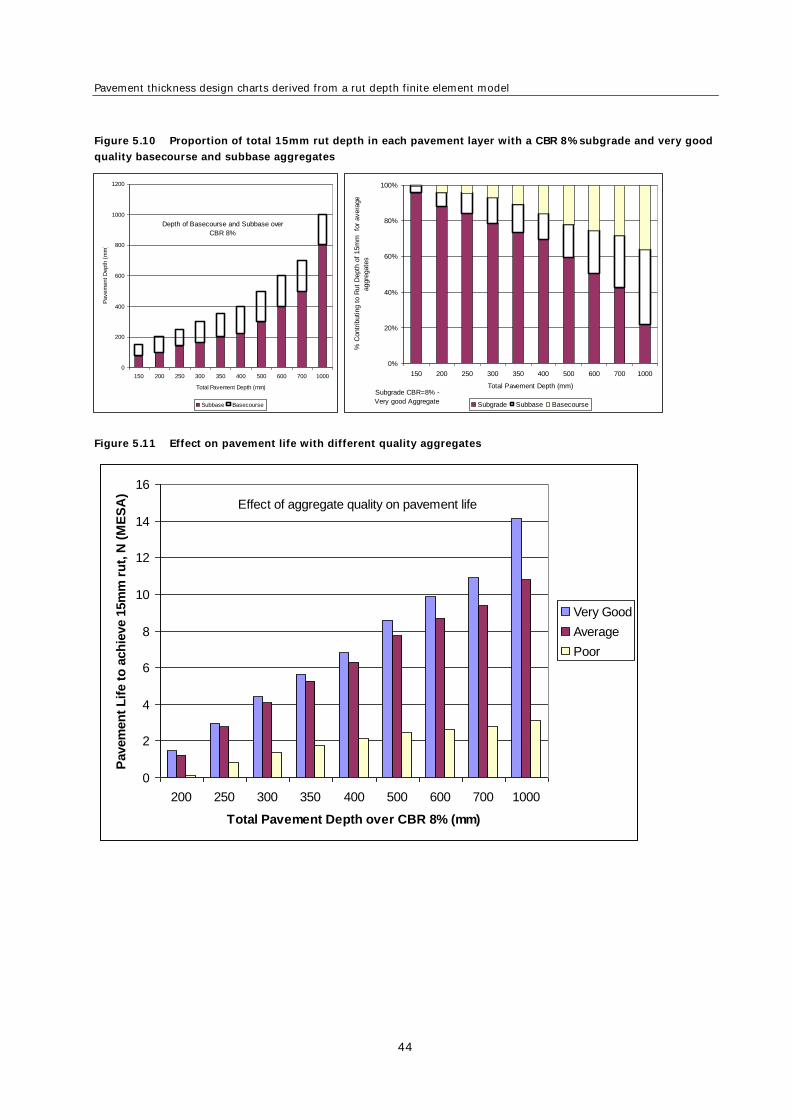
Pavement thickness design charts derived from a rut depth finite element model
44
Figure 5.10 Proportion of total 15mm rut depth in each pavement layer with a CBR 8% subgrade and very good
quality basecourse and subbase aggregates
Figure 5.11 Effect on pavement life with different quality aggregates
0%
20%
40%
60%
80%
100%
150 200 250 300 350 400 500 600 700 1000
Total Pavement Depth (mm)
% C
ontr
ibuting t
o R
ut
Depth
of
15m
m
for
avera
ge
aggre
gate
s
Subgrade Subbase Basecourse
Subgrade CBR=8% -
Very good Aggregate
0
200
400
600
800
1000
1200
150 200 250 300 350 400 500 600 700 1000
Total Pavement Depth (mm)
Pavem
ent D
epth
(m
m)
Subbase Basecourse
Depth of Basecourse and Subbase over
CBR 8%
0
2
4
6
8
10
12
14
16
200 250 300 350 400 500 600 700 1000
Total Pavement Depth over CBR 8% (mm)
Pavem
en
t L
ife t
o a
ch
ieve 1
5m
m r
ut,
N (
ME
SA
)
Very Good
Average
Poor
Effect of aggregate quality on pavement life

6 Granular pavement design charts based on rut depth prediction Arnold method
45
6 Granular pavement design charts based on rut depth prediction Arnold method
Only limited data in terms of subgrade strengths are available in the database of pavement lives found by
rut depth models. Therefore, to determine pavement lives for other subgrade types, some interpretation
between the CBR 10%, 8% and 2% is required (figures 6.1 and 6.2). It is assumed that the model to
interpret the lives for other subgrade types follows the same trend as the granular pavement design chart
in Austroads (2004, figure 8.4). The same ratio of pavement depths between each subgrade CBR values
found from the design chart in the Austroads guide was used to determine pavement thickness design
charts for other subgrade CBR values not tested in the triaxial apparatus. A design chart from rut depth
modelling for the full range of subgrade strengths is shown in figure 6.1 plotted using a linear scale.
Figure 6.2 uses a log scale which is more difficult to interpolate.
Figure 6.1 Pavement thickness design chart from rut depth modelling plotted on a linear scale
-1400.0
-1200.0
-1000.0
-800.0
-600.0
-400.0
-200.0
0.0
0.00E+00 2.00E+06 4.00E+06 6.00E+06 8.00E+06 1.00E+07 1.20E+07 1.40E+07 1.60E+07
Design Traffic, N (ESAs)
To
tal G
ran
ula
r P
av
em
en
t D
ep
th (
mm
) 30
20
15
10
9
8
7
6
5
4
3
2
Subgrade
CBR %
Average Quality Aggregate

Pavement thickness design charts derived from a rut depth finite element model
46
Figure 6.2 Pavement thickness design chart from rut depth modelling plotted on a log scale
A recommended conservative approach to these new design charts is to use the pavement thickness that
is the largest out of the Austroads (2004 figure 8.4) guide and the chart derived from rut depth
predictions. Combining the Austroads design chart and the rut depth predictions results in the design
chart shown in figures 6.3 and 6.4.
Figure 6.3 Pavement thickness design chart for average quality aggregate derived from Austroads (2004)
design guide and from rut depth modelling plotted on a linear scale
-1400.0
-1200.0
-1000.0
-800.0
-600.0
-400.0
-200.0
0.0
1.00E+05 1.00E+06 1.00E+07 1.00E+08
Design Traffic, N (ESAs)
To
tal G
ran
ula
r P
av
em
en
t D
ep
th (
mm
) 30
20
15
10
9
8
7
6
5
4
3
2
Subgrade
CBR %
Average Quality Aggregate
-1400
-1200
-1000
-800
-600
-400
-200
0
0.00E+00 2.00E+06 4.00E+06 6.00E+06 8.00E+06 1.00E+07 1.20E+07 1.40E+07 1.60E+07
Design Traffic, N (ESAs)
To
tal G
ran
ula
r P
av
em
en
t D
ep
th (
mm
) 30
20
15
10
9
8
7
6
5
4
3
2
Subgrade
CBR %
Austroads combined with rut
depth predictions
Average Quality Aggregate
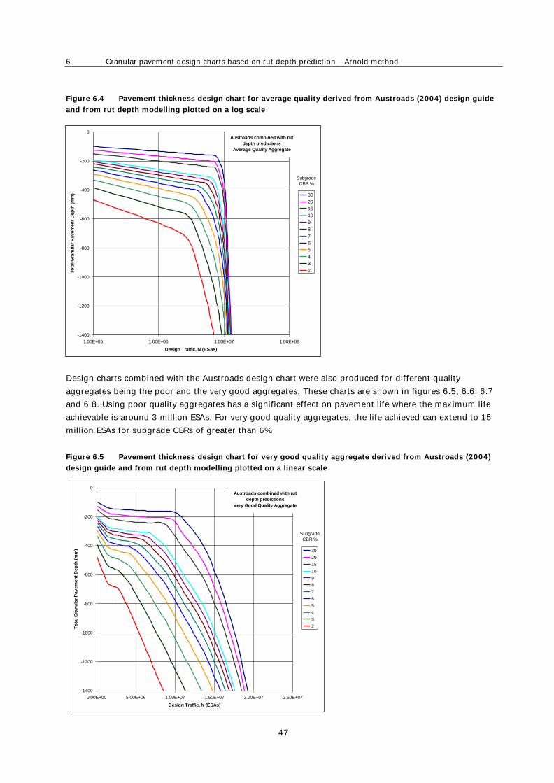
6 Granular pavement design charts based on rut depth prediction Arnold method
47
Figure 6.4 Pavement thickness design chart for average quality derived from Austroads (2004) design guide
and from rut depth modelling plotted on a log scale
Design charts combined with the Austroads design chart were also produced for different quality
aggregates being the poor and the very good aggregates. These charts are shown in figures 6.5, 6.6, 6.7
and 6.8. Using poor quality aggregates has a significant effect on pavement life where the maximum life
achievable is around 3 million ESAs. For very good quality aggregates, the life achieved can extend to 15
million ESAs for subgrade CBRs of greater than 6%.
Figure 6.5 Pavement thickness design chart for very good quality aggregate derived from Austroads (2004)
design guide and from rut depth modelling plotted on a linear scale
-1400
-1200
-1000
-800
-600
-400
-200
0
1.00E+05 1.00E+06 1.00E+07 1.00E+08
Design Traffic, N (ESAs)
To
tal G
ran
ula
r P
av
em
en
t D
ep
th (
mm
) 30
20
15
10
9
8
7
6
5
4
3
2
Subgrade
CBR %
Austroads combined with rut
depth predictions
Average Quality Aggregate
-1400
-1200
-1000
-800
-600
-400
-200
0
0.00E+00 5.00E+06 1.00E+07 1.50E+07 2.00E+07 2.50E+07
Design Traffic, N (ESAs)
To
tal G
ran
ula
r P
av
em
en
t D
ep
th (
mm
) 30
20
15
10
9
8
7
6
5
4
3
2
Subgrade
CBR %
Austroads combined with rut
depth predictions
Very Good Quality Aggregate

Pavement thickness design charts derived from a rut depth finite element model
48
Figure 6.6 Pavement thickness design chart for very good quality aggregate derived from Austroads (2004)
design guide and from rut depth modelling plotted on a log scale
Figure 6.7 Pavement thickness design chart for poor quality aggregate derived from Austroads (2004) design
guide and from rut depth modelling plotted on a linear scale
-1400
-1200
-1000
-800
-600
-400
-200
0
1.00E+05 1.00E+06 1.00E+07 1.00E+08
Design Traffic, N (ESAs)
To
tal G
ran
ula
r P
av
em
en
t D
ep
th (
mm
) 30
20
15
10
9
8
7
6
5
4
3
2
Subgrade
CBR %
Austroads combined with rut
depth predictions
Very Good Quality Aggregate
-1400
-1200
-1000
-800
-600
-400
-200
0
0.00E+00 5.00E+05 1.00E+06 1.50E+06 2.00E+06 2.50E+06 3.00E+06 3.50E+06 4.00E+06
Design Traffic, N (ESAs)
To
tal G
ran
ula
r P
av
em
en
t D
ep
th (
mm
) 30
20
15
10
9
8
7
6
5
4
3
2
Subgrade
CBR %
Austroads combined with rut
depth predictions
Poor Quality Aggregate
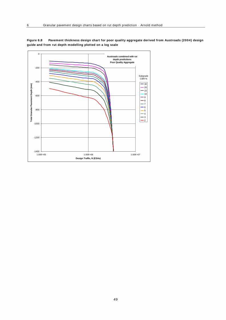
6 Granular pavement design charts based on rut depth prediction Arnold method
49
Figure 6.8 Pavement thickness design chart for poor quality aggregate derived from Austroads (2004) design
guide and from rut depth modelling plotted on a log scale
-1400
-1200
-1000
-800
-600
-400
-200
0
1.00E+05 1.00E+06 1.00E+07
Design Traffic, N (ESAs)
To
tal G
ran
ula
r P
av
em
en
t D
ep
th (
mm
) 30
20
15
10
9
8
7
6
5
4
3
2
Subgrade
CBR %
Austroads combined with rut
depth predictions
Poor Quality Aggregate
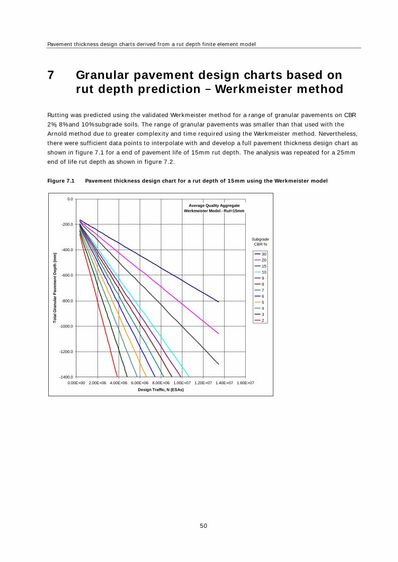
Pavement thickness design charts derived from a rut depth finite element model
50
7 Granular pavement design charts based on rut depth prediction Werkmeister method
Rutting was predicted using the validated Werkmeister method for a range of granular pavements on CBR
2%, 8% and 10% subgrade soils. The range of granular pavements was smaller than that used with the
Arnold method due to greater complexity and time required using the Werkmeister method. Nevertheless,
there were sufficient data points to interpolate with and develop a full pavement thickness design chart as
shown in figure 7.1 for a end of pavement life of 15mm rut depth. The analysis was repeated for a 25mm
end of life rut depth as shown in figure 7.2.
Figure 7.1 Pavement thickness design chart for a rut depth of 15mm using the Werkmeister model
-1400.0
-1200.0
-1000.0
-800.0
-600.0
-400.0
-200.0
0.0
0.00E+00 2.00E+06 4.00E+06 6.00E+06 8.00E+06 1.00E+07 1.20E+07 1.40E+07 1.60E+07
Design Traffic, N (ESAs)
To
tal G
ran
ula
r P
av
em
en
t D
ep
th (
mm
) 30
20
15
10
9
8
7
6
5
4
3
2
Subgrade
CBR %
Average Quality Aggregate
Werkmeister Model - Rut=15mm

7 Granular pavement design charts based on rut depth prediction Werkmeister method
51
Figure 7.2 Pavement thickness design chart for a rut depth of 25mm using the Werkmeister model for
average quality aggregate
-1400.0
-1200.0
-1000.0
-800.0
-600.0
-400.0
-200.0
0.0
0.00E+00 5.00E+06 1.00E+07 1.50E+07 2.00E+07 2.50E+07 3.00E+07
Design Traffic, N (ESAs)
To
tal G
ran
ula
r P
av
em
en
t D
ep
th (
mm
) 30
20
15
10
9
8
7
6
5
4
3
2
Subgrade
CBR %
Average Quality Aggregate
Werkmeister Model - Rut=25mm
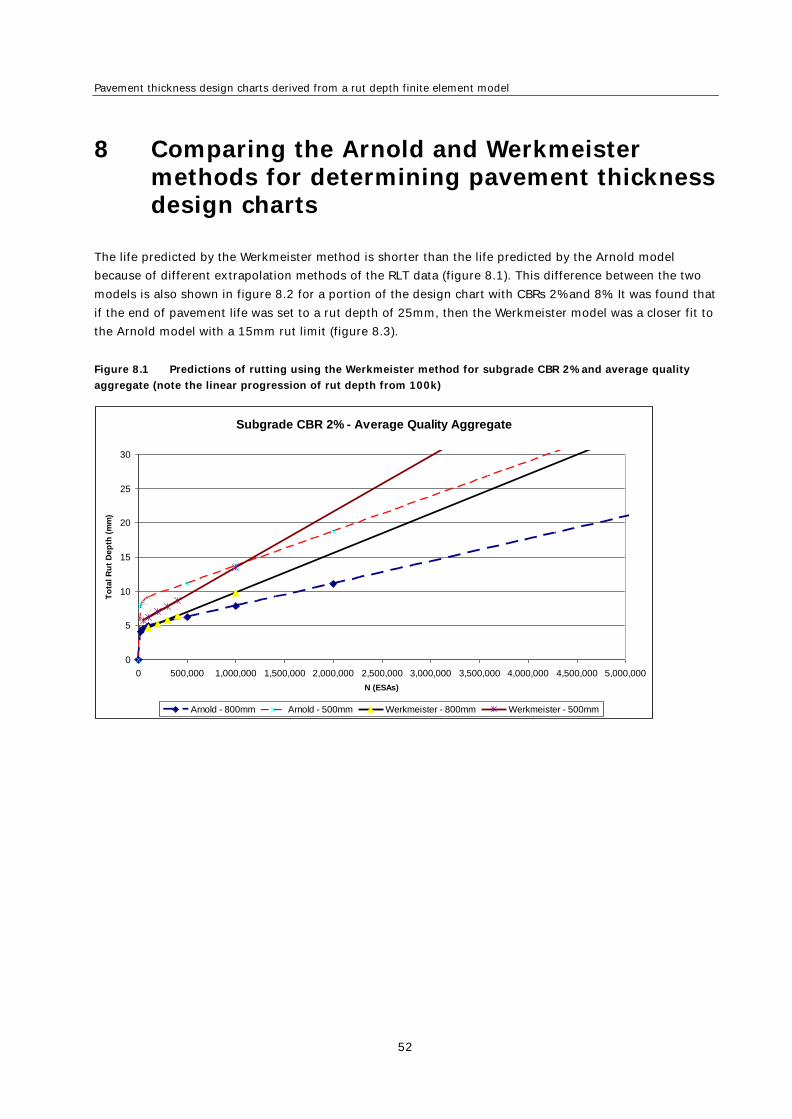
Pavement thickness design charts derived from a rut depth finite element model
52
8 Comparing the Arnold and Werkmeister methods for determining pavement thickness design charts
The life predicted by the Werkmeister method is shorter than the life predicted by the Arnold model
because of different extrapolation methods of the RLT data (figure 8.1). This difference between the two
models is also shown in figure 8.2 for a portion of the design chart with CBRs 2% and 8%. It was found that
if the end of pavement life was set to a rut depth of 25mm, then the Werkmeister model was a closer fit to
the Arnold model with a 15mm rut limit (figure 8.3).
Figure 8.1 Predictions of rutting using the Werkmeister method for subgrade CBR 2% and average quality
aggregate (note the linear progression of rut depth from 100k)
Subgrade CBR 2% - Average Quality Aggregate
0
5
10
15
20
25
30
0 500,000 1,000,000 1,500,000 2,000,000 2,500,000 3,000,000 3,500,000 4,000,000 4,500,000 5,000,000
N (ESAs)
To
tal
Ru
t D
ep
th (
mm
)
Arnold - 800mm Arnold - 500mm Werkmeister - 800mm Werkmeister - 500mm

8 Comparing the Arnold and Werkmeister methods
53
Figure 8.2 Pavement thickness design chart comparison between the Arnold and Werkmeister models for a
rut depth of 15mm
Figure 8.3 Pavement thickness design chart comparison between the Arnold (rut=15mm) and Werkmeister
(rut=25mm)
-1400.0
-1200.0
-1000.0
-800.0
-600.0
-400.0
-200.0
0.0
0.00E+00 2.00E+06 4.00E+06 6.00E+06 8.00E+06 1.00E+07 1.20E+07 1.40E+07 1.60E+07
Design Traffic, N (ESAs)
To
tal G
ran
ula
r P
av
em
en
t D
ep
th (
mm
)
8 - Werk
2 - Werk
2 - Arn
8 - Arn
Subgrade
CBR %
Average Quality Aggregate
Werkmeister and Arnold Model -
Rut=15mm
-1400.0
-1200.0
-1000.0
-800.0
-600.0
-400.0
-200.0
0.0
0.00E+00 5.00E+06 1.00E+07 1.50E+07 2.00E+07 2.50E+07 3.00E+07
Design Traffic, N (ESAs)
To
tal G
ran
ula
r P
av
em
en
t D
ep
th (
mm
)
2 - Arn
8 - Arn
2
8
Subgrade
CBR %
Average Quality Aggregate
Werkmeister (Rut=25mm) and
Arnold Model (Rut=15mm)

Pavement thickness design charts derived from a rut depth finite element model
54
On reviewing the Werkmeister rut depth predictions, it can be seen that they are linear with the same
slope after approximately 10,000 load cycles (figure 7.1). This is because the Werkmeister method uses
one relationship between permanent strain rate and elastic strain from one portion of the permanent
strain curve found from RLT testing. This one relationship has the effect of a linear increase in rutting and
is likely to predict a higher rut depth than would be expected to occur. In contrast, the Arnold method
uses five different relationships between stress and permanent strain rate for different portions of the
permanent strain curve found from RLT testing, being: 0 25,000; 25,000 50,000; 50,000 100,000;
100,000 500,000; 500,000 onwards linear using same slope as 100,000 to 500,000. This has the effect
of flattening the rutting curve with less rutting being calculated using the Arnold method (figure 8.1). It
would be possible to use the Werkmeister model also for different stages of the RLT curve as per the
Arnold method and thus for similar predictions in rut depth.
A current shortcoming of the Werkmeister method is the absence of a suitable model for the subgrade
soils. For all of the pavement cross-sections analysed, the Werkmeister model found most of the surface
rutting was in the granular layers regardless of the pavement depth even for a 200mm pavement on a
subgrade CBR of 2%. The Arnold method used a more suitable model for the subgrade and thus showed
that surface rutting was dominated by subgrade rutting for shallow pavement depths.

9 Conclusions
55
9 Conclusions
The design charts are produced from a range of assumptions that result in similar rut depth predictions to
those that actually occurred at the CAPTIF test track. Number of wheel passes at the test track are
relatively short (< 1.5 MESA) compared with design lives of state highways (approximately 10 MESA).
Therefore, aggregate shakedown which may occur in the field where after many applications load there is
no further rutting is not considered in the rut depth model validated with CAPTIF data. If shakedown or
partial shakedown was assumed, then the rutting model would follow a log or power function, that
continually decreases the rate of rutting with increasing load cycles. This would increase life significantly
and the maximum life obtainable for average quality granular pavements would likely be around 50 MESA.
The current assumption assumes a conservative linear rutting relationship after 0.5 MESA to follow the
trend of the CAPTIF data.
Despite possible errors in the rut depth predictions, the exercise was useful in demonstrating the relative
effect on pavement life for different qualities of aggregates and and showing that increasing the depth of
the aggregates did not always increase the pavement life. The results showed that after 6 MESA one or
more modified or bound pavement layers were required to limit rutting in the granular pavement layers.
RLT tests on subgrade, subbase and basecourse materials have enabled relationships to be determined
between permanent strain/rutting and stress (Arnold method) or elastic strain (Werkmeister method).
These relationships permit the calculation of rutting within each pavement material which is summed to
obtain a surface rut depth. CAPTIF pavements were used to validate and refine the assumptions used to
calculate the surface rut depths to ensure they were close to measured rut depths. The validated Arnold
and Werkmeister rut depth prediction models were then used to calculate rutting for a range of pavement
depths on CAPTIF subgrade soils with CBRs of 2%, 8% and 10%. Results of this analysis were assessed by
the number of ESAs to achieve a total surface rut depth defining the end of life. This information was used
to develop pavement thickness design charts from the rut depth predictions and compared to the chart for
granular pavements in Austroads (2004, figure 9.1). For low traffic volumes, the Austroads guide requires
thicker pavements, while for high traffic volumes the rut depth predictions show significantly thicker
pavements are required. In fact the rut depth predictions show there are traffic loading limits for granular
pavements at around 7 million ESA for the subgrade CBR 2% and 11 million ESAs for the subgrade CBR 8%
(figure 9.1). A reason for this is the significant amount of rutting that occurs in the aggregate layers for
the thicker pavement depths as shown in figure 9.2. Because rutting occurs within the granular layers,
adding more granular material does not decrease the amount of rutting and increase pavement life.

Pavement thickness design charts derived from a rut depth finite element model
56
Figure 9.1 Rut depth predictions in comparison with Austroads
Figure 9.2 Proportion of total 15mm rut depth in each pavement layer with a CBR 8% subgrade and average
quality basecourse and subbase aggregates
Rut depth predictions were repeated with different quality aggregates in terms of resistance to rutting
found from the RLT test. The effect of using very good unbound aggregates increased the maximum
pavement life from 11 million ESAs for average quality to 14 million ESAs for a subgrade with CBR 8%
(figure 9.3). However, when using poor quality aggregates the maximum life decreased to 3 million ESAs
(figure 9.3).
-1400
-1200
-1000
-800
-600
-400
-200
0
0.00E+00 2.50E+06 5.00E+06 7.50E+06 1.00E+07 1.25E+07 1.50E+07 1.75E+07 2.00E+07
Design Traffic, N (ESAs)
To
tal G
ran
ula
r P
av
em
en
t D
ep
th (
mm
)
2 - Arn
8 - Arn
2 - Werk
8 - Werk
2 - Austroads
8 - Austroads
Subgrade
CBR %
Average Quality Aggregate
Werkmeister (Rut=25mm) and
Arnold Model (Rut=15mm)
0%
20%
40%
60%
80%
100%
200 250 300 350 400 450 500 550 750 1000
Total Pavement Depth (mm)
% C
ontr
ibuting t
o R
ut
Depth
of
15m
m
for
avera
ge
aggre
gate
s
Subgrade Subbase Basecourse
Subgrade CBR=8% -
Average Aggregate
0
200
400
600
800
1000
1200
200 250 300 350 400 450 500 550 750 1000
Total Pavement Depth (mm)
Pavem
ent D
epth
(m
m)
Subbase Basecourse
Depth of Basecourse and Subbase over
CBR 8%

9 Conclusions
57
Figure 9.3 Effect on pavement life with different quality aggregates
Finally, a combined Austroads and rut depth prediction pavement thickness design chart was produced by
using the largest pavement thickness from the two methods as shown in figures 9.4 and 9.5. It is
recommended that this replace the Austroads (2004) figure 8.4.
Figure 9.4 Combining Austroads and rut depth predictions for subgrade CBR 8%
0
2
4
6
8
10
12
14
16
200 250 300 350 400 500 600 700 1000
Total Pavement Depth over CBR 8% (mm)
Pavem
en
t L
ife t
o a
ch
ieve 1
5m
m r
ut,
N (
ME
SA
)
Very Good
Average
Poor
Effect of aggregate quality on pavement life
-1400
-1200
-1000
-800
-600
-400
-200
0
1.00E+05 1.00E+06 1.00E+07 1.00E+08
Design Traffic, N (ESAs)
To
tal G
ran
ula
r P
av
em
en
t D
ep
th (
mm
)
Combined
Austroads, Fig 8.4
Rut Depth Prediction
Subgrade CBR = 8%Austroads combined with rut
depth predictions
Average Quality Aggregate

Pavement thickness design charts derived from a rut depth finite element model
58
Figure 9.5 Recommended pavement thickness design chart for average quality aggregate combining
Austroads and rut depth prediction
-1400
-1200
-1000
-800
-600
-400
-200
0
1.00E+05 1.00E+06 1.00E+07 1.00E+08
Design Traffic, N (ESAs)
To
tal G
ran
ula
r P
av
em
en
t D
ep
th (
mm
) 30
20
15
10
9
8
7
6
5
4
3
2
Subgrade
CBR %
Austroads combined with rut
depth predictions
Average Quality Aggregate

10 Recommendations
59
10 Recommendations
It is recommended that the findings of this research project (see figure 9.4) be implemented in the
New Zealand supplement to the Austroads pavement design guide (NZTA 2007) as shown in appendix C.
Appendix C also details the design method using a basecourse and sub-base strain criterion as developed
in a parallel project by Arnold and Werkmeister on the development of a basecourse/sub-base design
criterion. The aim of this parallel project was to develop basecourse and sub-base strain criteria for use
with CIRCLY pavement design that would obtain the same life as shown in the pavement thickness design
chart from rut depth modelling (figure 9.4). Use of basecourse and sub-base strain criteria is more
versatile as it allows options such as increasing asphalt cover and/or stabilising a pavement layer to be
investigated as alternative design options that will meet the design life. Initial use of these criteria should
be optional for a time period of two years to gather feedback on their use so the method can be further
validated and refined.

Pavement thickness design charts derived from a rut depth finite element model
60
11 References
AASHO (1962) The AASHO road test. Conference Proceedings: Special Report 73. Highway Research Board,
National Academy of Sciences National Research Council. Washington DC, USA.
Alabaster, D and A Fussell (2006) Fatigue design criteria for low noise surfaces on New Zealand roads.
Transfund NZ research report no.307.
Arnold, G (2004) Rutting of granular pavements. PhD thesis. University of Nottingham, Nottingham, UK.
Arnold, G, D Alabaster and B Steven (2001) Prediction of pavement performance from repeat load triaxial
tests on granular materials. Transfund NZ research report no.214. 120pp.
Arnold, G, D Alabaster and B Steven (2005) Effect on pavement wear of an increase in mass limits for
heavy vehicles. Land Transport NZ research report no.281.
Arnold, G, S Werkemeister and D Alabaster (2008) Performance tests for road aggregates and alternative
materials. Land Transport NZ research report no.335.
Austroads (2004) Pavement design. A guide to the structural design of road pavements. Sydney:
Austroads.
Austroads (2008) Technical basis of Austroads guide to pavement technology part 2: pavement structural
design. Austroads no. AP T98/08.
Benkelman, AC (1962) Structural deterioration of test pavements: flexible. The AASHO road test. Highway
Research Board Special Report 73.
Chan, FWK (1990) Permanent deformation resistance of granular layers in pavements, PhD thesis,
University of Nottingham, Nottingham, UK.
Davis, EH (1949) The California bearing ratio method for the design of flexible roads and runways,
Géotechnique 14: 249 63.
de Beer, M, C Fisher and FJ Jooste (2002) Evaluation of non-uniform tyre contact stresses on thin asphalt
pavements. Ninth International Conference on Asphalt Pavements, August 17 22, 2002, Copenhagen,
Denmark.
Douglas, R (2009) Tyre/road contact stresses measured and modelled in three coordinate directions. NZ
Transport Agency research report 384. 54pp and appendix.
George, HP and CA Gittoes (1959) Report to Permanent International Association of Road Congresses
(PIARC), Section 2, Question VI, Part A. Rio de Janeiro.
Jouve, P and S Guezouli (1993) Comparison and harmonized development of some finite element
programs. Flexible Pavements. Edited by A. Gomes Correia, Technical University of Lisbon. Proceedings
of the European Symposium Euroflex 1993, Lisbon, Portugal 20 22 September 1993.
Korkiala-Tanttu, L, R Laaksonen and J Törnqvist (2003) Effect of the spring and overload to the rutting of a
low-volume road. HVS-Nordic-research. Helsinki 2003. Finnish Road Administration. Finnra Reports
22/2003. 39pp and appendix.

11 References
61
Lekarp, F (1997) Permanent deformation behaviour of unbound granular materials; Licentiate Thesis,
Kungl Tekniska Högskolan, Sweden.
Little, PH (1993) The design of unsurfaced roads using geosynthetics, PhD thesis, Dept. of Civil
Engineering, University of Nottingham.
NZ Transport Agency (NZTA) NZ supplement to the Austroads pavement design guide. Accessed
September 2010. www.nzta.govt.nz/resources/nz-supplement-2004-austroads-pavement-
design/docs/supplement.pdf
Oeser, M (2004) Numerische Simulation des nichtlinearen Verhaltens flexibler mehrschichtiger
Verkehrswegebefestigungen, PhD thesis, University of Technology, Dresden, Germany.
Pidwerbesky, B (1996) Fundamental behaviour of unbound granular pavements subjected to various
loading conditions and accelerated trafficking. PhD thesis, University of Canterbury, Christchurch, New
Zealand.
Porter, OJ (1938) The preparation of subgrades, 18th Highway Research Board Meeting, Washington DC,
United States, pp324 31.
Rodway, B (1997) Going round in Circlies, Geomechanics Society Pavements Symposium, Sydney.
Semmelink, CJ, FJ Jooste and M de Beer (1997) Use of the K-mould in determination of the elastic and
shear properties of road materials for flexible pavements. 8th Int. Conf. on Asphalt Pavements, August,
Seattle, Washington, USA.
Snaith, MS, D McMullen, RJ Freer-Hewish and A Shein (1980) Flexible pavement analysis. Contracted report
to sponsors, European Research Office of the US Army.
Standards Australia (1995) AS 1289.6.8.1: Methods of testing soils for engineering purposes. Soil strength
and consolidation tests determination of the resilient modulus and permanent deformation of
granular unbound pavement materials. Sydney: Standards Australia.
Theyse, HL (2002) Stiffness, strength, and performance of unbound aggregate material: application of
South African HVS and laboratory results to California flexible pavements. University of California
Pavement Research Center.
Theyse, HL (2004) Mechanistic empirical design models for pavement subgrades. In Unbound aggregates
in roads. Proceedings of the 6th International Symposium UNBAR6: 229 238. Nottingham.
Thom, N and S Brown (1989) The mechanical properties of unbound aggregates from various sources.
Proceedings of the Third International Symposium on Unbound Aggregates in Roads, UNBAR3,
Nottingham, 11 13 April 1989.
Transit NZ (2005) TNZ B/02 Specification for construction of unbound granular pavement layers.
Wellington: Transit NZ.
Transit NZ (2006) TNZ M/4 Specification for basecourse aggregate. Wellington: Transit NZ.
Transit NZ (2007) TNZ T/15 specification for repeated load triaxial (RLT) testing of unbound and modified
road base aggregates. Wellington: Transit NZ.

Pavement thickness design charts derived from a rut depth finite element model
62
Vuong, BT and R Brimble (2000) Austroads repeated load triaxial test method determination of
permanent deformation and resilient modulus characteristics of unbound granular materials under
drained conditions. APRG 00/33 (MA) June.
Vuong, BT (2001) Improved performance-based material specifications and performance prediction
models for granular pavements. PhD thesis. Department of Civil and Geological Engineering, Faculty of
Engineering, RMIT University: Melbourne, Australia.
Wardle LJ (1980) Program CIRCLY, a computer program for the analysis of multiple complex loads on
layered anisotropic media.
Werkmeister S (2007) Prediction of pavement response using accelerated test results o
CAPTIF facility. Dresden, Germany: TU.

Appendix A: Repeated load triaxial test summary for subgrade soils
63
Appendix A: Repeated load triaxial test summary for subgrade soils

Pavement thickness design charts derived from a rut depth finite element model
64
RLT subgrade soil tests
RLT Test Single test q p E-Modulus
resilient
strain
permanet
strain rate
RLT
PS0026 # Subgrade Soil MC DD Lab CBR Date [kPa] [kPa] [kPa] [kPa] [MPa] [mm/m]
[Slope 25k to
50k %/1M]
1 Waikari Silty Clay 14.2 1.74 17 12/11/2007 A 68 85 17 74 78 89 0.050
..\..\RLT Testing\PS0026 Rut Depth Modelling Subgrades\1 PS0026_Test 1_Waik_ 14_11_07v1.xls B 234 277 43 249 127 259 0.107
C 218 310 92 249 163 503 0.312
D 201 340 139 248 149 863 1.118
E 119 210 91 149 107 755 0.379
F 60 102 42 74 81 394 -0.038
G 102 241 139 149 104 1242 1.984
H 185 371 186 247 155 1143 0.838
I 169 401 232 246 137 1619 2.666
J 152 429 277 245 138 1927 3.491
NA Waikari Silty Clay 7.8 1.68 50 8/11/2007 RLT Test Not Conducted as Too strong - CBR = 50%
1a & 1b Waikari Silty Clay 11.9 1.72 25 31/01/2008 A 50 150 100 84 80 1190 2.313
B 50 170 120 90 79 1458 2.395
C 50 190 140 97 82 1655 2.514
D 50 210 160 103 84 1838 2.627
E 50 230 180 110 87 2011 2.900
F 50 250 200 117 90 2176 2.871
2 Waikari Silty Clay 11.9 1.72 25 4/02/2008 A 100 350 250 183 121 2021 2.348
B 100 400 300 200 128 2301 3.206
C 100 450 350 217 130 2651 3.977
D 100 500 400 233 136 2903 4.208
E 100 550 450 250 141 3158 4.645
3 Waikari Silty Clay 11.9 1.72 25 7/02/2008 A 200 350 150 250 135 1077 1.249
B 200 400 200 267 135 1447 1.972
C 200 450 250 283 141 1738 2.401
D 200 500 300 300 149 1979 2.684
E 200 550 350 317 158 2188 2.901
F 200 600 400 333 168 2346 3.201
G 200 650 450 350 178 2491 2.971

Appendix A: Repeated load triaxial test summary for subgrade soils
65
RLT Test Single test q p E-Modulus
resilient
strain
permanet
strain rate
RLT
PS0026 # Subgrade Soil MC DD Lab CBR Date [kPa] [kPa] [kPa] [kPa] [MPa] [mm/m]
[Slope 25k to
50k %/1M]
13A Todd Clay 30 1.425 2.5 approx. 21/01/2008 A 200 210 10 203 125 39 0.945
28.3 1.54.5 (CBR 13/2/08) B 200 215 15 205 122 82 0.845
C 200 220 20 207 110 136 1.382
D 200 230 30 210 64 391 1.444
E 200 240 40 213 42 1107 2.093
F 200 250 50 217 17 2678 12.071
12 Todd Clay 30 1.425 2.5 approx. 17/01/2008 A 100 110 10 103 97 51 1.056
28.3 1.54.5 (CBR 13/2/08) B 100 115 15 105 91 109 1.034
C 100 120 20 107 74 201 1.027
D 100 130 30 110 34 729 1.340
E 100 140 40 113 18 1982 2.593
F 100 150 50 117 15 3032 153.233
7 Todd Clay 19.4 1.6 17 8/11/2007 A 68 85 17 74 181 38 0.081
B 234 277 43 249 172 191 0.148
C 218 310 92 249 127 647 0.429
D 201 340 139 248 88 1457 0.816
E 119 210 91 149 107 758 0.211
F 60 102 42 74 185 173 -0.069
G 102 241 139 149 85 1510 0.404
H 185 371 186 247 60 2959 3.445
8 Todd Clay 24.2 1.58 8 23/11/2007 A 68 85 17 74 154 45 0.168
B 234 277 43 249 165 200 3.159
C 218 310 92 249 127 816 2.830
11 Todd Clay 30 1.425 2.5 approx. 16/01/2008 A 50 60 10 54 77 64 0.742
28.3 1.54.5 (CBR 13/2/08) B 50 65 15 55 64 155 0.813
C 50 70 20 57 46 328 0.880
D 50 80 30 60 21 1205 1.656
E 50 90 40 63 14 2510 45.715
10a Todd Clay 30 1.425 2.5 approx. 14/12/2008 A 243 265 22 250 61 277 0.279
28.3 1.54.5 (CBR 13/2/08)

Pavement thickness design charts derived from a rut depth finite element model
66
21 Very Fine Pumice Test Pit # 6 @ 2m11.7 1.06 25 9/05/2008 A 50 60 10 53 52 95 0.057
B 50 100 50 67 55 814 0.555
C 50 150 100 83 71 1333 1.457
D 50 200 150 100 84 1722 1.702
E 50 250 200 117 95 2055 2.124
F 50 300 250 133 105 2340 2.883
G 50 350 300 150 113 2615 3.229
H 50 400 350 167 119 2900 5.152
22 Very Fine Pumice Test Pit # 6 @ 2m11.7 1.06 25 9/05/2008 A 100 200 100 133 101 937 0.658
B 100 300 200 167 106 1847 2.370
C 100 350 250 183 111 2214 2.930
D 100 400 300 200 116 2532 4.186
E 100 450 350 217 120 2872 7.750
F 100 500 400 233 124 3181 11.011
70 Waikari Silty Clay - CBR 12%? A 50 200 150 100 84 1736 3.793
B 50 250 200 117 90 2177 4.492
C 50 300 250 133 96 2541 5.074
D 50 350 300 150 103 2869 6.058
E 50 400 350 167 110 3142 17.761
F 50 449 399 183 118 3348 0.000
52 Todd Clay CBR = 5% A 200 225 25 208 205 97 -0.015
B 200 250 50 217 175 257 0.181
C 200 300 100 233 74 1278 0.861
D 200 325 125 242 48 2489 2.241
E 200 350 150 250 48 2997 0.000
F 200 400 200 267 37 5241
51 Todd Clay CBR = 5% A 100 150 50 117 171 264 0.407
B 100 200 100 133 83 1145 1.092
C 100 250 150 150 65 2220 0.000
D 100 300 200 167 43 4474 0.000
E 100 350 250 183 15 0.000

Appendix A: Repeated load triaxial test summary for subgrade soils
67
50 Todd Clay CBR = 5% A 50 100 50 67 114 393 0.730
B 50 150 100 83 53 1783 2.048
C 50 200 150 100 44 3273 0.000
41 Drury Test Pit # 1 CBR + 6% A 100 150 50 117 150 300 0.567
B 100 200 100 133 128 742 0.943
C 100 250 150 150 98 1488 0.000
D 100 299 199 166 44 4383 0.000
E 100 349 249 183 0 0 0.000
40 Drury Test Pit # 1 CBR = 6% A 50 100 50 67 145 310 0.461
B 50 150 100 83 123 775 0.906
C 50 250 200 117 41 4705 0.000
D 50 299 249 133 37 2201 0.000
33 Pumice CBR=25% A 200 300 100 233 140 677 0.480
B 200 400 200 267 137 1425 1.639
C 200 450 250 283 139 1766 2.114
D 200 500 300 300 144 2055 2.646
E 200 550 350 317 148 2331 3.531
F 200 600 400 333 151 2608 5.035
56 Todd Clay 26.5% MC - cell =50kPa
57 Todd Clay 25.5% MC - cell = 100kPa
58 Todd Clay 25.5% MC - cell = 200kPa

Pavement thickness design charts derived from a rut depth finite element model
68
0
0.5
1
1.5
2
2.5
3
0 50000 100000 150000 200000 250000 300000 350000 400000
1a & 1b Waikari Clay, cell = 50kpa, vert = 100 - 200kPa, CBR=25%
0
0.5
1
1.5
2
2.5
3
0 50000 100000 150000 200000 250000 300000 350000 400000
1 Waikari Clay, cell = various, vert = 100 - 200kPa, CBR=17%
0
0.5
1
1.5
2
2.5
3
0 50000 100000 150000 200000 250000 300000 350000 400000
2 Waikari Clay, cell = 100kpa, vert = various, CBR=25%

Appendix A: Repeated load triaxial test summary for subgrade soils
69
0
0.5
1
1.5
2
2.5
3
0 50000 100000 150000 200000 250000 300000 350000 400000
3 Waikari Clay, cell = 200kpa, vert = various, CBR=25%
0
0.5
1
1.5
2
2.5
3
0 50000 100000 150000 200000 250000 300000 350000 400000
13A Todd Clay, cell = 200kpa, vert = various, CBR=2.5% or 4.5%
0
0.5
1
1.5
2
2.5
3
0 50000 100000 150000 200000 250000 300000 350000 400000
14 Todd Clay, cell = 100kpa, vert = various, CBR=2.5% or 4.5%

Pavement thickness design charts derived from a rut depth finite element model
70
0
0.5
1
1.5
2
2.5
3
0 50000 100000 150000 200000 250000 300000 350000 400000
7 Todd Clay, cell = various, vert = various, CBR=17%
0
0.5
1
1.5
2
2.5
3
0 50000 100000 150000 200000 250000 300000 350000 400000
8 Todd Clay, cell = various, vert = various, CBR=2.5% (or 4.5%)
0
0.5
1
1.5
2
2.5
3
0 50000 100000 150000 200000 250000 300000 350000 400000
11 Todd Clay, cell = various, vert = various, CBR=2.5% (or 4.5%)

Appendix A: Repeated load triaxial test summary for subgrade soils
71
0
0.5
1
1.5
2
2.5
3
0 50000 100000 150000 200000 250000 300000 350000 400000
10a Todd Clay, cell = various, vert = various, CBR=2.5% (or 4.5%)

Pavement thickness design charts derived from a rut depth finite element model
72
Appendix B: Repeated load triaxial testing and rut depth modelling technical note
Repeated load triaxial testing and rut depth modelling for pavement materials (granular, modified,
local, recycled, waste, stabilised subgrade)
Dr Greg Arnold, PaveSpec Ltd (email: [email protected] web: www.rltt.co.nz (please check web for latest
contact details and laboratory location)
What is repeated load triaxial (RLT) testing?
The RLT apparatus applies repetitive loading on cylindrical
materials for a range of specified stress conditions, the
output is deformation (shortening of the cylindrical
sample) versus number of load cycles (usually 50,000) for
a particular set of stress conditions. Multi-stage RLT tests
are used to obtain deformation curves for a range of
stress conditions to develop models for predicting rutting.
Resilient modulus information can also be obtained for
pavement design in CIRCLY and finite element models.
Figure B1 RLT apparatus and setup
Figure B2 Typical output from permanent strain RLT
testing
Analysis of RLT testing results rut depth
modelling
The method developed by Dr Arnold in his Doctorate
studies at the University of Nottingham, UK is used to
interpret the results to predict the rut depth in a
pavement. First step is to develop a mathematical
relationship between stress (both vertical and horizontal)
with permanent strain rate (slope of each deformation
curves (figure B2), eg % deformation per 1 million load
cycles).
Figure B3 Fitting the permanent strain rate model to
RLT testing results
Figure B4 Rut depth prediction from RLT testing for
CAPTIF (accelerated pavement test) trial
0.0
0.5
1.0
1.5
2.0
0.00 0.20 0.40 0.60 0.80 1.00
Principal Stress Difference, q (MPa)
Perm
an
en
t str
ain
rate
(%
/1M
)
(25k t
o 1
00k
)
0.075
0.150
0.250
0.075
0.150
0.250
CAPTIF 3
R2 = 0.92
Mean Principal Stress, p (MPa)
3
1
3 = 2
cell
pressure
3
1
2q = 1 – 3
p = 1/3( 1+ 2+ 3)
erate = e(a) e(bp) e(cq) - e(a) e(bp)
0.0
0.5
1.0
1.5
2.0
0.00 0.20 0.40 0.60 0.80 1.00
Principal Stress Difference, q (MPa)
Perm
an
en
t str
ain
rate
(%
/1M
)
(25k t
o 1
00k
)
0.075
0.150
0.250
0.075
0.150
0.250
CAPTIF 3
R2 = 0.92
Mean Principal Stress, p (MPa)
3
1
3 = 2
cell
pressure
3
1
2q = 1 – 3
p = 1/3( 1+ 2+ 3)
0.0
0.5
1.0
1.5
2.0
0.00 0.20 0.40 0.60 0.80 1.00
Principal Stress Difference, q (MPa)
Perm
an
en
t str
ain
rate
(%
/1M
)
(25k t
o 1
00k
)
0.075
0.150
0.250
0.075
0.150
0.250
CAPTIF 3
R2 = 0.92
Mean Principal Stress, p (MPa)
3
1
3 = 2
cell
pressure
3
1
2q = 1 – 3
p = 1/3( 1+ 2+ 3)
3
1
3 = 2
cell
pressure
3
1
2q = 1 – 3
p = 1/3( 1+ 2+ 3)
erate = e(a) e(bp) e(cq) - e(a) e(bp)
0
0.2
0.4
0.6
0.8
1
0 50,000 100,000 150,000 200,000 250,000 300,000
Number of load cycles [-]
Perm
anent str
ain
[%
]
AB
CD
E
F
0
2
4
6
8
10
12
14
16
0 200 400 600 800 1000 1200 1400
Wheel Passes ('000s)
Avera
ge D
efo
rmation (
mm
)
1 - 50 kN VSD
Best fit, Horiz.=0kPa, Defmn. 25k= 0.56mm
Calculated - original
ID: 1: 50kN
Load = 50 kN

Appendix B: Repeated load triaxial testing and rut depth modelling technical note
73
Next step is to use a finite element model (to model the
non-linear elastic behaviour of a pavement material and to
avoid discontinuities as occurs in CIRCLY which results in
high tensile stresses) to compute the stresses (both
vertical and horizontal underneath a standard axle load
(8.2 tonne dual tyred axle or higher if designing for ports
etc). Stresses are exported into a spreadsheet to calculate
the deformation rate at depth increments in the pavement
from the permanent strain model (figure B3). Results
showed very good predictions of rutting that occurred at
CAPTIF (figure 4) (Arnold 2004).
Applications for RLT testing and rut depth
modelling
Preventing early failure
Recent research has shown that even if your aggregate
complies with M4 that they do not perform equally. The
aggregate may fail by shear (figure B5) within six months
after the pavement has been constructed especially if it
gets wet. The RLT testing can quickly identify aggregates
where there may be a risk of this occurring as often the
sample fails before the completion of all the stress stages
(figure B2).
Figure B5 Shear failure in aggregate layer
Modified/stabilised materials for high trafficked
roads
Small quantities of cement, lime or other additive are
classified as a modified aggregate in the New Zealand
supplement to the Austroads pavement design guide.
Modified aggregates are recommended in the New Zealand
supplement for use for high trafficked state highways as
an economical alternative to structural asphalt. Using the
RLT testing will identify the most appropriate amount of
additive and using rut depth modelling can predict the
amount of extra life that can be obtained through
modification compared with the source aggregate.
Modified/stabilised marginal local materials as a lower
cost to TNZ M4 (and may perform better!)
RLT testing and rut depth modelling allow any material
that does not comply with a current specification to be
assessed as suitable or not for the chosen application in
the pavement.
This allows a local material non-compliant with the
specifications to be modified by say adding cement to be
approved for use. The NZTA is in the process of
developing an RLT testing method and associated analysis
to approve use of other materials on state highways.
Local materials for local roads
Footpaths, tennis courts, cul-de-sacs, low trafficked local
roads do not need to use TNZ M/4 basecourse aggregate
meant for state highways. In fact M4 is difficult to lay and
compact for these small local jobs. RLT testing and rut
depth prediction for the required application can allow say
a local but dirty aggregate to be assessed as suitable for
low trafficked situations and footpaths.
Waste and recycled materials
Waste or recycled materials like glass and reclaimed
asphalt mixed with aggregate or otherwise can be tested
in the RLT apparatus with rut depth modelling to
determine appropriate applications as pavement base
material.
PaveSpec Ltd
Dr Greg Arnold is the Director of PaveSpec Ltd which along
with offering specialist pavement advice and design is a
company that has just recently purchased a state of the art
repeated load triaxial apparatus for testing pavement
materials.
Soil
Aggregate
Soil
Aggregate

Pavement thickness design charts derived from a rut depth finite element model
74
Appendix C: Recommended additions to the New Zealand supplement to the 2004 Austroads pavement design guide
This appendix sets out suggested changes to the NZ supplement to the 2004 Austroads pavement design
guide. The heading numbers relate to the same chapters and sections in the Austroads guide.
Chapter 6 Pavement materials
6.1 General
(Add)
Designers are encouraged to use new design strain criteria for use with CIRCLY have been developed for
New Zealand granular and cemented materials. Section 6.2.2 details strain criteria to use for unbound and
modified granular materials while section 6.4.2 details tensile strain criteria for cemented granular materials.
These new design criteria are material specific and require repeated load triaxial (RLT) test data as per NZTA
T/15 and/or flexural tensile strength from beam breakage tests or derived from indirect tensile strength
tests. Presumptive values are given but should be used cautiously with the design being refined by using test
data on actual materials used in the project.
In the absence of CIRCLY and new design criterion then figure 8.4 in the Austroads (2004) guide should be
replaced with figures 6.1a and 6.1b for designing thin-surfaced granular pavements. These new design charts
were developed from rut depth modelling carried out by Arnold and Werkmeister in 2010.

Appendix C: Recommended additions to the New Zealand supplement to the 2004 Austroads pavement design guide
75
Figure 6.1a Recommended pavement thickness design chart for average quality aggregate combining Austroads
(2004) and rut depth predictions
-1400
-1200
-1000
-800
-600
-400
-200
0
1.00E+05 1.00E+06 1.00E+07 1.00E+08
Design Traffic, N (ESAs)
To
tal G
ran
ula
r P
av
em
en
t D
ep
th (
mm
) 30
20
15
10
9
8
7
6
5
4
3
2
Subgrade
CBR %
Austroads combined with rut
depth predictions
Average Quality Aggregate

Pavement thickness design charts derived from a rut depth finite element model
76
Figure 6.1b Pavement thickness design chart for average quality aggregate derived from Austroads (2004) design
guide and from rut depth modelling plotted on a linear scale
6.2 Unbound granular materials
6.2.1 Introduction
6.2.2 Basecourse and subbase design strain criteria for CIRCLY pavement design
For basecourse aggregate covered with a thin surface of less than 50mm then the vertical compressive strain
at the bottom but within the basecourse layer is limited by equation 6.1. For cases where the cover is greater
than 50mm then the basecourse will be treated as a subbase for design as per equation 6.2.
NBC
= M*[(a.f.kBC
/resilient strain bottom of BC)^expBC
] (Equation 6.1)
where:
NBC
=life of basecourse in equivalent standard axles (ESAs)
-1400
-1200
-1000
-800
-600
-400
-200
0
0.00E+00 2.00E+06 4.00E+06 6.00E+06 8.00E+06 1.00E+07 1.20E+07 1.40E+07 1.60E+07
Design Traffic, N (ESAs)
To
tal G
ran
ula
r P
av
em
en
t D
ep
th (
mm
) 30
20
15
10
9
8
7
6
5
4
3
2
Subgrade
CBR %
Austroads combined with rut
depth predictions
Average Quality Aggregate

Appendix C: Recommended additions to the New Zealand supplement to the 2004 Austroads pavement design guide
77
a = constant to adjust strain at bottom of basecourse to a maximum strain in the basecourse
a = 1/( BC depth (mm) x 0.00905) derived from equation 5.1
f = 2.0 - adjustment factor determined from validation to ensure calculated life from stain criterion is equal to
life calculated from rut depth modelling
kBC
= constant found from RLT testing (NZTA T/15 and appendix D, presumptive values shown in table 6.1)
expBC
= constant found from RLT testing (NZTA T/15 and appendix D, presumptive values shown in table 6.1)
resilient strain bottom of BC = resilient strain at the bottom of the basecourse layer as calculated using
CIRCLY.
M= pavement depth multiplier due to reduced rutting in subgrade (table 6.2)
The life of the sub-base aggregate layer is found from equation 6.2:
NSB
= M*[(f.kSB
/resilient strain top of SB)^expSB
] (Equation 6.2)
Where:
NSB =life of sub-base or basecourse if covered by more than 50mm of bound material in ESAs;
f = 2.0 adjustment factor determined from validation to ensure calculated life from stain criterion is equal to
life calculated from rut depth modelling
kSB = constant found from RLT testing (NZTA T/15 and appendix D, presumptive values shown in table 6.1)
expSB = constant found from RLT testing (NZTA T/15 and appendix D, presumptive values shown in table 6.1)
resilient strain top of SB = resilient strain at the top of the subbase layer.
M= pavement depth multiplier due to reduced rutting in subgrade (table 6.1)

Pavement thickness design charts derived from a rut depth finite element model
78
Table 6.1 Aggregate life multiplier from pavement depth resulting in reduced rutting in the subgrade
Subgrade
CBR%
Pavement depth (mm) when
aggregate life influences
(D)
Aggregate life multiplier
M
(ie multiply computed life by M) up to a
maximum of M=1.8.
2 1000 M = Total pavement depth/D
3 854
4 750
5 670
6 604
7 548
8 500
9 458
10 420
11 385
12 354
13 325
14 298
15 273
It is recommended that designers conduct their own RLT tests to obtain the constants in the design strain
criterions for subbase and basecourse aggregates, while the range of values found unbound aggregates from
the Pavespec Ltd database of RLT tests are shown in table 6.2. The use of modified and cemented granular
materials will require independent RLT tests to determine appropriate constants for the design stain criterion
as detailed in Appendix D and NZTA T/15. Further, the constants in table 6.2 were derived from dry tests in
the RLT apparatus. A separate design is needed if the case for saturation of the granular layers is considered
using equation constants derived from saturated RLT tests.

Appendix C: Recommended additions to the New Zealand supplement to the 2004 Austroads pavement design guide
79
Table 6.2 Constants and exponent values for CIRCLY design strain criterions
N = (f.a.k/micro-
strain)exp
f=2.0 (see Eqn. 6.1
and 6.2)
Sub-base linear
Extrapolation to 3.3%
(NB: K for Circly = b*2
see appendix A)
Basecourse linear
Extrapolation to 3.3%
(NB: K for Circly = b*2
see appendix A)
Strain criterion b exp b exp
Upper (best) 80,000 3.4 700,000 2.4
Middle 66,000 3.4 400,000 2.4
Lower (poor) 55,000 3.4 250,000 2.4
(see below for details how to obtain these constants from RLT tests)
6.3 Modified granular materials
(Add)
A design procedure for these materials has now been developed for use in CIRCLY using design strain
criterion for basecourse and/or sub-base granular materials as per equations 6.1 and 6.2 above, except
material specific equation constants will be derived from RLT tests on modified granular materials. Due to
increase deformation resistance with modified materials then this should result in an increase in pavement life
when compared with unbound granular materials, particularly in a saturated condition. Nevertheless, the extra
life from modified materials maybe restricted by its fatigue life as determined by equation 6.3 in section
6.4.2 Cemented materials . The fatigue life of modified materials must be considered in design if any
improvements in life beyond an unbound granular material are being considered.

Pavement thickness design charts derived from a rut depth finite element model
80
Appendix D: Method to determine vertical compressive strain criterion from repeated load triaxial test data
Step 1:
Determine the average slope (%/1M) as per table D1 as measured in the RLT test and resulting load cycles to
achieve a permanent strain limit (3.3%).
Table D1 Calculation of average permanent strain slope from 6-stage RLT test
RLT test stage
(table 2)
2Permanent
strain (%)
(see figure 1)
1Permanent strain slope
(%/1M) (slopes)
A
Number of load cycles (N) to achieve a
permanent strain of 3.3%
N = 3.3/A * 106
Stage A P25k
=(P50k
-P25k
)/0.025M = 3.3 / [(P50k
-P25k
)/0.025M]
P50k
Stage B P75k
=(P100k
-P75k
)/0.025M = 3.3 / [(P100k
-P75k
)/0.025M]
P100k
Stage C P125k
=(P150k
-P125k
)/0.025M = 3.3 / [(P150k
-P125k
)/0.025M]
P150k
Stage D P175k
=(P200k
-P175k
)/0.025M = 3.3 / [(P200k
-P175k
)/0.025M]
P200k
Stage E P225k
=(P250k
-P225k
)/0.025M = 3.3 / [(P250k
-P225k
)/0.025M]
P250k
Stage F P275k
=(P300k
-P275k
)/0.025M = 3.3 / [(P300k
-P275k
)/0.025M]
P300k
Average = Pavg
= ( Slopes)/6
Note: 1: If any of the loading stages do not complete the full amount of loading cycles because the deformation limit of
1.0% was achieved then table 5 calculations will not strictly apply. In this situation the average tangential permanent strain
slope achieved is used in replace of the value from 25,000 to 50,000 load cycles.
2: Permanent strain values for any given load cycle are the average of the previous 10 readings in the RLT test to account
for any noise in the data.

Appendix D: Method to determine vertical compressive strain criterion from repeated load triaxial test data
81
Figure D1 Permanent strain points for determination of permanent strain slopes
Step 2:
Determine the relationship between life (N, table D1) and resilient elastic strain as recorded in the RLT test.
Then plot log (N) versus log (micro-strain) and determine line of best fit for slope and intercept constants (a
and b) as shown in figure D1.
Transformation of Multi-Stage RLT Data to Single Stages
0
0.1
0.2
0.3
0.4
0.5
0.6
0.7
0.8
0.9
1
0 25,000 50,000 75,000 100,000 125,000 150,000 175,000 200,000 225,000 250,000 275,000 300,000
Number of load cycles [-]
Perm
an
en
t str
ain
[%
]
Stage A Stage B Stage C Stage D Stage E Stage F
P25k
P50k
P75k
P100k
P125k
P150k
A
B
C
D
E
F
P175k
P200k
P225k
P250k
P275k
P300k

Pavement thickness design charts derived from a rut depth finite element model
82
Table D2 Calculation of average permanent strain slope from 6-stage RLT test
Log10 both sides and calculate
slope (a) and intercept (b) (see
figure 1)
Log( ) = a.log( ) + b
RLT test
stage (table
2)
Vertical
resilient
strain
Number of load cycles (N) to achieve a
permanent strain of 3.3%
N = 3.3/A * 106
Log ( ) Log (N)
Stage A A
= 3.3 / [(P50k
-P25k
)/0.025M]
Stage B B = 3.3 / [(P
100k-P
75k)/0.025M]
Stage C C
= 3.3 / [(P150k
-P125k
)/0.025M]
Stage D D = 3.3 / [(P
200k-P
175k)/0.025M]
Stage E E
= 3.3 / [(P250k
-P225k
)/0.025M]
Stage F F = 3.3 / [(P
300k-P
275k)/0.025M]
Figure D2 Example plot of log(N) versus log(strain) for calculating line of best fit for slope and intercept
constants (a and b)
log( ) = -0.4052log(N) + 5.5488
R2 = 0.8877
0
0.5
1
1.5
2
2.5
3
3.5
5.50 5.70 5.90 6.10 6.30 6.50 6.70 6.90 7.10 7.30 7.50
Log (N)
Lo
g (
resil
ien
t m
icro
-str
ain
)
log( ) = a.log(N) + b

Appendix D: Method to determine vertical compressive strain criterion from repeated load triaxial test data
83
Step 3:
From line of best fit for slope and intercept constants (a and b) as shown in figure D2 in step 2 determine
power law exponent and constant for strain criterion uses in CIRCLY (equation D1):
N = (K/micro-strain)exp Equation D1
Where,
N = Fatigue life in equivalent standard axles (ESAs)
K = [10b ]. f
b = Intercept constant, b in log(N) vs log(strain) relationship (figure
D1)
f = 2.0 - adjustment factor determined from validation to ensure
calculated life from stain criterion is equal to life calculated from
rut depth modelling
exp = (1/a)*(-1)
a = Slope constant, a in log(N) vs log(strain) relationship (figure D2)
micro-strain = Vertical compressive resilient strain at the top of the subbase
aggregate layer or at a depth of 80mm from the surface in the
basecourse layer.

Pavement thickness design charts derived from a rut depth finite element model
84