Recent Advances in Hierarchical Reinforcement Learning

Andrew G. BartoSridhar Mahadevan

Autonomous Learning LaboratoryDepartment of Computer Science

University of Massachusetts, Amherst MA 01003

Abstract

Reinforcement learning is bedeviled by the curse of dimensionality: the number of parameters tobe learned grows exponentially with the size of any compact encoding of a state. Recent attempts tocombat the curse of dimensionality have turned to principled ways of exploiting temporal abstraction,where decisions are not required at each step, but rather invoke the execution of temporally-extendedactivities which follow their own policies until termination. This leads naturally to hierarchical controlarchitectures and associated learning algorithms. We review several approaches to temporal abstractionand hierarchical organization that machine learning researchers have recently developed. Common tothese approaches is a reliance on the theory of semi-Markov decision processes, which we emphasize in ourreview. We then discuss extensions of these ideas to concurrent activities, multiagent coordination, andhierarchical memory for addressing partial observability. Concluding remarks address open challengesfacing the further development of reinforcement learning in a hierarchical setting.

1

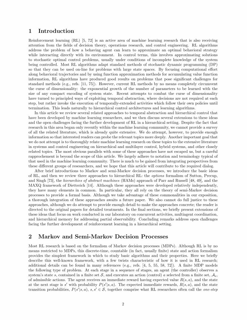
1 Introduction

Reinforcement learning (RL) [5, 72] is an active area of machine learning research that is also receivingattention from the fields of decision theory, operations research, and control engineering. RL algorithmsaddress the problem of how a behaving agent can learn to approximate an optimal behavioral strategywhile interacting directly with its environment. In control terms, this involves approximating solutionsto stochastic optimal control problems, usually under conditions of incomplete knowledge of the systembeing controlled. Most RL algorithms adapt standard methods of stochastic dynamic programming (DP)so that they can be used on-line for problems with large state spaces. By focusing computational effortalong behavioral trajectories and by using function approximation methods for accumulating value functioninformation, RL algorithms have produced good results on problems that pose significant challenges forstandard methods (e.g., refs. [11, 75]). However, current RL methods by no means completely circumventthe curse of dimensionality: the exponential growth of the number of parameters to be learned with thesize of any compact encoding of system state. Recent attempts to combat the curse of dimensionalityhave turned to principled ways of exploiting temporal abstraction, where decisions are not required at eachstep, but rather invoke the execution of temporally-extended activities which follow their own policies untiltermination. This leads naturally to hierarchical control architectures and learning algorithms.

In this article we review several related approaches to temporal abstraction and hierarchical control thathave been developed by machine learning researchers, and we then discuss several extensions to these ideasand the open challenges facing the further development of RL in a hierarchical setting. Despite the fact thatresearch in this area began only recently within the machine learning community, we cannot provide a surveyof all the related literature, which is already quite extensive. We do attempt, however, to provide enoughinformation so that interested readers can probe the relevant topics more deeply. Another important goal thatwe do not attempt is to thoroughly relate machine learning research on these topics to the extensive literaturein systems and control engineering on hierarchical and multilayer control, hybrid systems, and other closelyrelated topics. The most obvious parallels with some of these approaches have not escaped us, but a carefulrapprochement is beyond the scope of this article. We largely adhere to notation and terminology typical ofthat used in the machine learning community. There is much to be gained from integrating perspectives fromthese different groups of resesarchers, and we hope that this article will contribute to the required dialog.

After brief introductions to Markov and semi-Markov decision processes, we introduce the basic ideasof RL, and then we review three approaches to hierarchical RL: the options formalism of Sutton, Precup,and Singh [73], the hierarchies of abstract machines (HAMs) approach of Parr and Russell [48, 49], and theMAXQ framework of Dietterich [14]. Although these approaches were developed relatively independently,they have many elements in common. In particular, they all rely on the theory of semi-Markov decisionprocesses to provide a formal basis. Although we take advantage of these commonalities in our exposition,a thorough integration of these approaches awaits a future paper. We also cannot do full justice to theseapproaches, although we do attempt to provide enough detail to make the approaches concrete; the reader isdirected to the original papers for detailed treatments. In the final sections, we briefly present extensions ofthese ideas that focus on work conducted in our laboratory on concurrent activities, multiagent coordination,and hierarchical memory for addressing partial observability. Concluding remarks address open challengesfacing the further development of reinforcement learning in a hierarchical setting.

2 Markov and Semi-Markov Decision Processes

Most RL research is based on the formalism of Markov decision processes (MDPs). Although RL is by nomeans restricted to MDPs, this discrete-time, countable (in fact, usually finite) state and action formalismprovides the simplest framework in which to study basic algorithms and their properties. Here we brieflydescribe this well-known framework, with a few twists characteristic of how it is used in RL research;additional details can be found in many references (e.g., refs. [4, 5, 55, 58, 72]). A finite MDP modelsthe following type of problem. At each stage in a sequence of stages, an agent (the controller) observes asystem’s state s, contained in a finite set S, and executes an action (control) a selected from a finite set, As,of admissible actions. The agent receives an immediate reward having expected value R(s, a), and the stateat the next stage is s′ with probability P (s′|s, a). The expected immediate rewards, R(s, a), and the statetransition probabilities, P (s′|s, a), s, s′ ∈ S, together comprise what RL researchers often call the one-step

2

model of action a.A (stationary, stochastic) policy π : S× ∪s∈S As → [0, 1], with π(s, a) = 0 for a 6∈ As, specifies that the

agent executes action a ∈ As with probability π(s, a) whenever it observes state s. For any policy π ands ∈ S, V π(s) denotes the expected infinite-horizon discounted return from s given that the agent uses policyπ. Letting st and rt+1 denote the state at stage t and the immediate reward for acting at stage t,1 this isdefined as:

V π(s) = E{rt+1 + γrt+2 + γ2rt+3 + · · · |st = s, π},

where γ, 0 ≤ γ < 1, is a discount factor. V π(s) is the value of s under π, and is V π the value functioncorresponding to π.

This is a finite, infinite-horizon, discounted MDP. The objective is to find an optimal policy, i.e., apolicy, π∗, that maximizes the value of each state. The unique optimal value function, V ∗, is the valuefunction corresponding to any of the optimal policies. Most RL research addresses discounted MDPs sincethey comprise the simplest class of MDPs, and here we restrict attention to discounted problems. However,RL algorithms have also been developed for MDPs with other definitions of return, such as average rewardMDPs [39, 62].

Playing important roles in many RL algortihms are action-value functions, which assign values to ad-missible state-action pairs. Given a policy π, the value of (s, a), a ∈ As, denoted Qπ(s, a), is the expectedinfinite-horizon discounted return for executing a in state s and thereafter following π:

Qπ(s, a) = E{rt+1 + γrt+2 + γ2rt+3 + · · · |st = s, at = a, π}. (1)

The optimal action-value function, Q∗, assigns to each admissible state-action pair (s, a) the expected infinite-horizon discounted return for executing a in s and thereafter following an optimal policy. Action-valuefunctions for other definitions of return are defined analogously.

Dynamic Programming (DP) algorithms exploit the fact that value functions satisfy various Bellmanequations, such as:

V π(s) =∑

a∈Asπ(s, a)[R(s, a) + γ

∑

s′

P (s′|s, a)V π(s′)],

andV ∗(s) = max

a∈As[R(s, a) + γ

∑

s′

P (s′|s, a)V ∗(s′)], (2)

for all s ∈ S. Analogous equations exist for Qπ and Q∗. For example, the Bellman equation for Q∗ is:

Q∗(s, a) = R(s, a) + γ∑

s′

P (s′|s, a) maxa′∈As′

Q∗(s′, a′), (3)

for all s ∈ S, a ∈ As.As an example DP algorithm, consider value iteration, which successively approximates V ∗ as follows.

At each iteration k, it updates an approximation Vk of V ∗ by applying the following operation for each states:

Vk+1(s) = maxa∈As

[R(s, a) + γ∑

s′

P (s′|s, a)Vk(s′)]. (4)

We call this operation a backup because it updates a state’s value by transferring to it information aboutthe approximate values of its possible successor states. Applying this backup operation once to each state isoften called a sweep. Starting with an arbitrary initial function V0, the sequence {Vk} produced by repeatedsweeps converges to V ∗. A similar algorithm exists for successively approximating Q∗ using the followingbackup:

Qk+1(s, a) = R(s, a) + γ∑

s′∈SP (s′|s, a) max

a′∈As′Qk(s′, a′). (5)

Given V ∗, an optimal policy is any policy that for each s assigns non-zero probability only to thoseactions that realize the maximum on the right-hand side of (4). Similarly, given Q∗, an optimal policy is

1We follow Sutton and Barto [72] in denoting the reward for the action at stage t by rt+1 instead of the more usual rt.

3

any policy that for each s assigns non-zero probability only to the actions that maximize Q∗(s, ·). Thesemaximizing actions are often called greedy actions, and a policy defined in this way is a (stochastic) greedypolicy. Given sufficiently close approximations of V ∗ and Q∗ obtained by value iteration, then, optimalpolicies are taken to be the corresponding greedy policies. Note that finding greedy actions via Q∗ does notrequire access to the one-step action models (the R(s, a) and P (s′|s, a)) as it does when only V ∗ is available,where the right-hand side of (4) has to be evaluated. This is one of the reasons that action-value functionsplay a significant role in RL.

In an MDP, only the sequential nature of the decision process is relevant, not the amount of time thatpasses between decision stages. A generalization of this is the semi-Markov decision process (SMDP) inwhich the amount of time between one decision and the next is a random variable, either real- or integer-valued. In the real-valued case, SMDPs model continuous-time discrete-event systems (e.g., refs. [40, 55]). Ina discrete-time SMDP [26] decisions can be made only at (positive) integer multiples of an underlying timestep. In either case, it is usual to treat the system as remaining in each state for a random waiting time [26],at the end of which an instantaneous transition occurs to the next state. Due to its relative simplicity, thediscrete-time SMDP formulation underlies most approaches to hierarchical RL, but there are no significantobstacles to extending these approaches to the continuous-time case.

Let the random variable τ denote the (positive) waiting time for state s when action a is executed. Thetransition probabilities generalize to give the joint probability that a transition from state s to state s′ occursafter τ time steps when action a is executed. We write this joint probability as P (s′, τ |s, a). The expectedimmediate rewards, R(s, a), (which must be bounded) now give the amount of discounted reward expectedto accumulate over the waiting time in s given action a. The Bellman equations for V ∗ and Q∗ become

V ∗(s) = maxa∈As

[R(s, a) +∑

s′,τ

γτP (s′, τ |s, a)V ∗(s′)], (6)

for all s ∈ S; and

Q∗(s, a) = R(s, a) +∑

s′,τ

γτP (s′, τ |s, a) maxa′∈As′

Q∗(s′, a′), (7)

for all s ∈ S and a ∈ As. DP algorithms correspondingly extend to SMDPs (e.g., refs. [26, 55]).

3 Reinforcement Learning

DP algorithms have complexity polynomial in the number of states, but they still require prohibitive amountsof computation for large state sets, such as those that result from discretizing multi-dimensional continuousspaces or representing state sets consisting of all possible configurations of a finite set of structural elements(e.g., possible configurations of a backgammon board [75]). Many methods have been proposed for approx-imating MDP solutions with less effort than required by conventional DP, but RL methods are novel intheir use of Monte Carlo, stochastic approximation, and function approximation techniques. Specifically, RLalgorithms combine some, or all, of the following features:

1. Avoid the exhaustive sweeps of DP by restricting computation to states on, or in the neighborhoodof, multiple sample trajectories, either real or simulated. Because computation is guided along sam-ple trajectories, this approach can exploit situations in which many states have low probabilities ofoccurring in actual experience.

2. Simplify the basic DP backup by sampling. Instead of generating and evaluating all of a state’s possibleimmediate successors, estimate a backup’s effect by sampling from the appropriate distribution.

3. Represent value functions and/or policies more compactly than lookup-table representations by usingfunction approximation methods, such as linear combinations of basis functions, neural networks, orother methods.

Features 1 and 2 reflect the nature of the approximations usually sought when RL is used. Instead ofpolicies that are close to optimal uniformly over the entire state space, RL methods arrive at non-uniformapproximations that reflect the behavior of the agent. The agent’s policy does not need high precision in

4

states that are rarely visited. Feature 3 is the least understood aspect of RL, but results exist for thelinear case (notably ref. [81]) and numerous examples illustrate how function approximation schemes thatare nonlinear in the adjustable parameters (e.g., multilayer nerual networks) can be effective for difficultproblems (e.g., refs. [11, 40, 64, 75]).

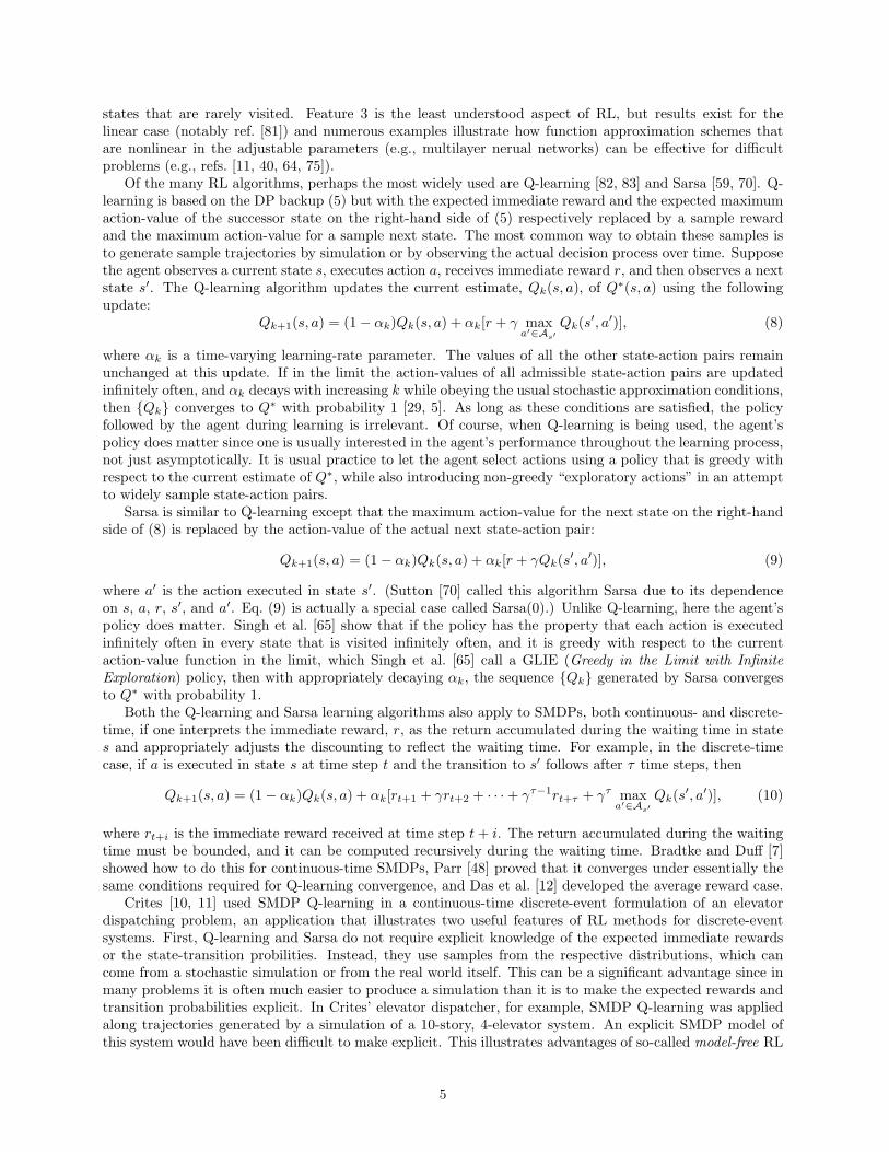
Of the many RL algorithms, perhaps the most widely used are Q-learning [82, 83] and Sarsa [59, 70]. Q-learning is based on the DP backup (5) but with the expected immediate reward and the expected maximumaction-value of the successor state on the right-hand side of (5) respectively replaced by a sample rewardand the maximum action-value for a sample next state. The most common way to obtain these samples isto generate sample trajectories by simulation or by observing the actual decision process over time. Supposethe agent observes a current state s, executes action a, receives immediate reward r, and then observes a nextstate s′. The Q-learning algorithm updates the current estimate, Qk(s, a), of Q∗(s, a) using the followingupdate:

Qk+1(s, a) = (1− αk)Qk(s, a) + αk[r + γ maxa′∈As′

Qk(s′, a′)], (8)

where αk is a time-varying learning-rate parameter. The values of all the other state-action pairs remainunchanged at this update. If in the limit the action-values of all admissible state-action pairs are updatedinfinitely often, and αk decays with increasing k while obeying the usual stochastic approximation conditions,then {Qk} converges to Q∗ with probability 1 [29, 5]. As long as these conditions are satisfied, the policyfollowed by the agent during learning is irrelevant. Of course, when Q-learning is being used, the agent’spolicy does matter since one is usually interested in the agent’s performance throughout the learning process,not just asymptotically. It is usual practice to let the agent select actions using a policy that is greedy withrespect to the current estimate of Q∗, while also introducing non-greedy “exploratory actions” in an attemptto widely sample state-action pairs.

Sarsa is similar to Q-learning except that the maximum action-value for the next state on the right-handside of (8) is replaced by the action-value of the actual next state-action pair:

Qk+1(s, a) = (1− αk)Qk(s, a) + αk[r + γQk(s′, a′)], (9)

where a′ is the action executed in state s′. (Sutton [70] called this algorithm Sarsa due to its dependenceon s, a, r, s′, and a′. Eq. (9) is actually a special case called Sarsa(0).) Unlike Q-learning, here the agent’spolicy does matter. Singh et al. [65] show that if the policy has the property that each action is executedinfinitely often in every state that is visited infinitely often, and it is greedy with respect to the currentaction-value function in the limit, which Singh et al. [65] call a GLIE (Greedy in the Limit with InfiniteExploration) policy, then with appropriately decaying αk, the sequence {Qk} generated by Sarsa convergesto Q∗ with probability 1.

Both the Q-learning and Sarsa learning algorithms also apply to SMDPs, both continuous- and discrete-time, if one interprets the immediate reward, r, as the return accumulated during the waiting time in states and appropriately adjusts the discounting to reflect the waiting time. For example, in the discrete-timecase, if a is executed in state s at time step t and the transition to s′ follows after τ time steps, then

Qk+1(s, a) = (1− αk)Qk(s, a) + αk[rt+1 + γrt+2 + · · ·+ γτ−1rt+τ + γτ maxa′∈As′

Qk(s′, a′)], (10)

where rt+i is the immediate reward received at time step t+ i. The return accumulated during the waitingtime must be bounded, and it can be computed recursively during the waiting time. Bradtke and Duff [7]showed how to do this for continuous-time SMDPs, Parr [48] proved that it converges under essentially thesame conditions required for Q-learning convergence, and Das et al. [12] developed the average reward case.

Crites [10, 11] used SMDP Q-learning in a continuous-time discrete-event formulation of an elevatordispatching problem, an application that illustrates two useful features of RL methods for discrete-eventsystems. First, Q-learning and Sarsa do not require explicit knowledge of the expected immediate rewardsor the state-transition probilities. Instead, they use samples from the respective distributions, which cancome from a stochastic simulation or from the real world itself. This can be a significant advantage since inmany problems it is often much easier to produce a simulation than it is to make the expected rewards andtransition probabilities explicit. In Crites’ elevator dispatcher, for example, SMDP Q-learning was appliedalong trajectories generated by a simulation of a 10-story, 4-elevator system. An explicit SMDP model ofthis system would have been difficult to make explicit. This illustrates advantages of so-called model-free RL

5

algorithms such as Q-learning and Sarsa, meaning that they do not need access to explicit representationsof the expected immediate reward function and the state-transition probabilities. Importantly, however, RLis not restricted to such model-free methods [72, 5].

RL algorithms that estimate action-values, such as Q-learning and Sarsa, have a second advantage whenapplied to discrete-event systems. As mentioned in Section 2, finding optimal actions via Q∗ does notrequire access to the one-step action models (the R(s, a) and P (s′|s, a)) as it does when only V ∗ is available.That is, a one-step ahead search is not needed to determine optimal actions. In many problems involvingdiscrete-event systems, such as the elevator dispatching problem, it is not clear how to conduct a one-stepahead search since the next event can occur at any of an infinite number of times in the future. The use ofaction-values eliminates this difficulty.

Finally, we point out that in our brief presentation of RL algorithms we assumed that it was possibleto explicitly store values for every state, or action-values for every state-action pair. This is obviously notfeasible for large-scale problems, and extensions of these algorithms need to be considered that adjust theparameters of parametric representations of value functions. It is relatively easy to produce such extensions,although, as we mentioned above, the theory of their behavior still contains many open questions which arebeyond the scope of this article.

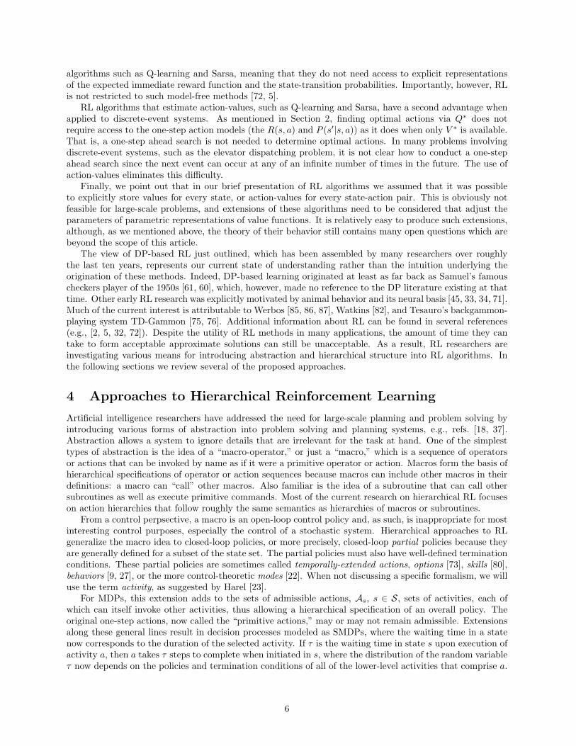
The view of DP-based RL just outlined, which has been assembled by many researchers over roughlythe last ten years, represents our current state of understanding rather than the intuition underlying theorigination of these methods. Indeed, DP-based learning originated at least as far back as Samuel’s famouscheckers player of the 1950s [61, 60], which, however, made no reference to the DP literature existing at thattime. Other early RL research was explicitly motivated by animal behavior and its neural basis [45, 33, 34, 71].Much of the current interest is attributable to Werbos [85, 86, 87], Watkins [82], and Tesauro’s backgammon-playing system TD-Gammon [75, 76]. Additional information about RL can be found in several references(e.g., [2, 5, 32, 72]). Despite the utility of RL methods in many applications, the amount of time they cantake to form acceptable approximate solutions can still be unacceptable. As a result, RL researchers areinvestigating various means for introducing abstraction and hierarchical structure into RL algorithms. Inthe following sections we review several of the proposed approaches.

4 Approaches to Hierarchical Reinforcement Learning

Artificial intelligence researchers have addressed the need for large-scale planning and problem solving byintroducing various forms of abstraction into problem solving and planning systems, e.g., refs. [18, 37].Abstraction allows a system to ignore details that are irrelevant for the task at hand. One of the simplesttypes of abstraction is the idea of a “macro-operator,” or just a “macro,” which is a sequence of operatorsor actions that can be invoked by name as if it were a primitive operator or action. Macros form the basis ofhierarchical specifications of operator or action sequences because macros can include other macros in theirdefinitions: a macro can “call” other macros. Also familiar is the idea of a subroutine that can call othersubroutines as well as execute primitive commands. Most of the current research on hierarchical RL focuseson action hierarchies that follow roughly the same semantics as hierarchies of macros or subroutines.

From a control perpsective, a macro is an open-loop control policy and, as such, is inappropriate for mostinteresting control purposes, especially the control of a stochastic system. Hierarchical approaches to RLgeneralize the macro idea to closed-loop policies, or more precisely, closed-loop partial policies because theyare generally defined for a subset of the state set. The partial policies must also have well-defined terminationconditions. These partial policies are sometimes called temporally-extended actions, options [73], skills [80],behaviors [9, 27], or the more control-theoretic modes [22]. When not discussing a specific formalism, we willuse the term activity, as suggested by Harel [23].

For MDPs, this extension adds to the sets of admissible actions, As, s ∈ S, sets of activities, each ofwhich can itself invoke other activities, thus allowing a hierarchical specification of an overall policy. Theoriginal one-step actions, now called the “primitive actions,” may or may not remain admissible. Extensionsalong these general lines result in decision processes modeled as SMDPs, where the waiting time in a statenow corresponds to the duration of the selected activity. If τ is the waiting time in state s upon execution ofactivity a, then a takes τ steps to complete when initiated in s, where the distribution of the random variableτ now depends on the policies and termination conditions of all of the lower-level activities that comprise a.

6

To the best of our knowledge (and as pointed out by Parr [48]), the approach most closely related to this inthe control literature is that of Forestier and Varaiya [20], which we discuss briefly in Section 4.2.

4.1 Options

Sutton, Precup, and Singh [73] formalize this approach to including activities in RL with their notion of anoption. Starting from a finite MDP, which we call the core MDP, the simplest kind of option consists of a(stationary, stochastic) policy π : S× ∪s∈S As → [0, 1], a termination condition β : S → [0, 1], and an inputset I ⊆ S. The option 〈I, π, β〉 is available in state s if and only if s ∈ I. If the option is executed, thenactions are selected according to π until the option terminates stochastically according to β. For example,if the current state is s, the next action is a with probability π(s, a), the environment makes a transition tostate s′, where the option either terminates with probability β(s′) or else continues, determining the nextaction a′ with probability π(s′, a′), and so on. When the option terminates, the agent can select anotheroption.

It is usual to assume that for any state in which an option can continue, it can also be initiated, thatis, {s : β(s) < 1} ⊆ I. This implies that an option’s policy only needs to be defined over its input set I.Note that any action of the core MDP, a primitive action a ∈ ∪s∈SAs, is also an option, called a one-stepoption, with I = {s : a ∈ As} and β(s) = 1 for all s ∈ S. Sutton et al. [73] give the example of an optionnamed open-the-door for a hypothetical robot control system. This option consists of a policy for reaching,grasping and turning the door knob, a termination condition for recognizing that the door has been opened,and an input set restricting execution of open-the-door to states in which a door is within reach.

An option of the type just defined is called a Markov option because its policy is Markov, that is, it setsaction probabilities based solely on the current state of the core MDP. To allow more flexibility, especiallywith respect to hierarchical architectures, one must include semi-Markov options whose policies can set actionprobabilities based on the entire history of states, actions, and rewards since the option was initiated [73].Semi-Markov options include options that terminate after a pre-specified number of time steps, and mostimportantly, they are needed when policies over options are considered, i.e., policies µ : S×∪s∈S Os → [0, 1],where Os is the set of admissible options for state s (which can include all the one-step options correspondingto the admissible primitive actions in As).

A policy µ over options selects option o in state s with probability µ(s, o); o’s policy in turn selectsother options until o terminates. The policy of each of these selected options selects other options, and soon. Expanding each option down to primitive actions, we see that any policy over options, µ, determinesa conventional policy of the core MDP, which Sutton et al. [73] call the flat (i.e, non-hierarchical) policycorresponding to µ, denoted flat(µ). Flat policies corresponding to policies over options are generally notMarkov even if all the options are Markov. The probability of a primitive action at any time step depends onthe current core state plus the policies of all the options currently involved in the hierarchical specification.This dependence is made more explicit in the work of Parr [48] and Dietterich [14], which we discuss below.Using this machinery (made precise by Precup [52]), one can define hierarchical options as triples 〈I, µ, β〉,where I and β are the same as for Markov options but µ is a semi-Markov policy over options.

Value functions for option policies can be defined in terms of value functions of semi-Markov flat policies.For a semi-Markov flat policy π:

V π(s) = E{rt+1 + γrt+2 + · · ·+ γτ−1rt+τ + · · · |E(π, s, t)},

where E(π, s, t) is the event of π being initiated at time t in s. Note that this value can depend on the completehistory from t onwards, but not on events earlier than t since π is semi-Markov. Given this definition forflat policies, V µ(s), the value of s for a policy µ over options, is defined to be V flat(µ)(s). Similarly, one candefine the option-value function for µ as follows:

Qµ(s, o) = E{rt+1 + γrt+2 + · · ·+ γτ−1rt+τ + · · · |E(oµ, s, t)},

where oµ is the semi-Markov policy that follows o until it terminates after τ time steps and then continuesaccording to µ.

Adding any set of semi-Markov options to a core finite MDP yields a well-defined discrete-time SMDPwhose actions are the options and whose rewards are the returns delivered over the course of an option’s

7

execution. Since the policy of each option is semi-Markov, the distributions defining the next state (the stateat an option’s termination), waiting time, and rewards depend only on the option executed and the statein which its execution was initiated. Thus, all of the theory and algorithms applicable to SMDPs can beappropriated for decision making with options.

In their effort to treat options as much as possible as if they were conventional single-step actions, Suttonet al. [73] introduced the interesting concept of a multi-time model of an option that generalizes the single-step model consisting of R(s, a) and P (s′|s, a), s, s′ ∈ S, of a conventional action a. For any option o, letE(o, s, t) denote the event of o being initiated in state s at time t. Then the reward part of the multi-timemodel of o for any s ∈ S is:

R(s, o) = E{rt+1 + γrt+2 + · · ·+ γτ−1rt+τ |E(o, s, t)},

where t+ τ is the random time at which o terminates. The state-prediction part of the model of o for s is:

P (s′|s, o) =

∞∑

τ=1

p(s′, τ)γτ ,

for all s ∈ S, where p(s′, τ) is the probability that the o terminates in s′ after τ steps when initiated in states. Though not itself a probability, P (s′|s, o) is a combination of the probability that s′ is the state in whicho terminates together with a measure of how delayed that outcome is in terms of γ.

The quantities R(s, o) and P (s′|s, o) respectively generalize the reward and transition probabilities,R(s, a) and P (s′|s, a), of the usual MDP in such a way that one can write a generalized form of the Bellmanoptimality equation. If V ∗O denotes the optimal value function over an option set O, then

V ∗O(s) = maxo∈Os

[R(s, o) +∑

s′

P (s′|s, o)V ∗O(s′)], (11)

which reduces to the usual Bellman optimality equation (2) if all the options are one-step options (β(s) = 1,s ∈ S). A Bellman equation analogous to (3) can be written for Q∗O:

Q∗O(s, o) = R(s, o) +∑

s′

P (s′|s, o) maxo′∈Os′

Q∗O(s′, o′), (12)

for all s ∈ S and o ∈ Os.The system of equations (11) and (12) can be solved respectively for V ∗O and Q∗O, exactly or approximately,

using methods that generalize the usual DP and RL algorithms [54]. For example, the DP backup analogousto (5) for computing option-values is:

Qk+1(s, o) = R(s, o) +∑

s′∈SP (s′|s, o) max

o′∈Os′Qk(s′, o′),

and the corresponding Q-learning update analogous to (8) is:

Qk+1(s, o) = (1− αk)Qk(s, o) + αk[r + γτ maxo′∈Os′

Qk(s′, o′)]. (13)

This update is applied upon the termination of o at state s′ after executing for τ time steps, and r is thereturn accumulated during o’s execution. This is the specialization of SMDP Q-learning given by (10) tothe SMDP that results from adding options to an MDP. It reduces to conventional Q-learning when allthe options are one-step options. In addition to refs. [52, 73], see refs. [54, 53, 48] for discussion of thisformulation and its relation to conventional SMDP theory.

As in the case of conventional MDPs, given V ∗O or Q∗O, optimal policies over options can be determinedas (stochastic) greedy policies. If each set of admissible options, Os, s ∈ S, contains one-step optionscorresponding to all of the primitive actions a ∈ As of the core MDP, then it is clear that the optimalpolicies over options are the same as the optimal policies for the core MDP (since primitive actions give themost refined degree of control). On the other hand, if some of the primitive actions are not available asone-step options, then optimal policies over the set of available options are in general suboptimal policies ofthe core MDP.

8

The theory described above all falls within conventional SMDP theory, which is specialized by the focuson semi-Markov options. A shortcoming of this is that the internal structure of an option is not readilyexploited. Precup [52] writes:

SMDP methods apply to options, but only when they are treated as opaque indivisible units.Once an option has been selected, such methods require that its policy be followed until theoption terminates. More interesting and potentially more powerful methods are possible bylooking inside options and by altering their internal structure. —Precup [52] p. 58.

For example, the Q-learning update (13) for options does nothing until an option terminates (and so doesnot apply to non-terminating options), and it only applies to one option at a time. This is the motivationfor intra-option learning methods which allow learning useful information before an option terminates andcan be used for multiple options simultaneously. For example, a variant of Q-learning, called one-step intra-option Q-learning [52], works as follows. Suppose (primitive) action at is taken in st, and the next state andimmediate reward are respectively st+1 and rt+1. Then for every Markov option o = 〈I, π, β〉 whose policycould have selected at according to the same distribution π(st, ·), this update is applied:

Qk+1(st, o) = (1− αk)Qk(st, o) + αk[rt+1 + γUk(st, o)], (14)

whereUk(s, o) = (1− β(s))Qk(s, o) + β(s) max

o′∈OQk(s, o′),

which is an estimate of the value of state-option pair (s, o) upon arrival in state s. In the case of deterministicoption policies, for example, this update is applied to all options whose policies select at in st whether thatoption was executing or not. If all the options in O are deterministic and Markov, then for every option inO this converges to Q∗O with probability 1, provided the αk decay appropriately and that in the limit everyprimitive action is executed infinitely often in every state [52].

Although its utility for hierarchical RL is limited due to its restriction to Markov options, one-step intra-option Q-learning is one example of a class of methods that take advantage of the structure of the core MDP.Related methods have been developed for estimating multi-time models of many options simultaneously byexploiting Bellman-like equations relating the components R(s, a) and P (s′|s, a) of multi-time models forsuccessive states. Results also exist on interrupting an option’s execution in favor of an option more highlyvalued for the current state, and for adjusting an option’s termination condition to allow the longest expectedexecution without sacrificing performance. See Sutton et al. [73] and Precup [52] for details on these andother option-related algorithms and illustrations of their performance.

The primary motivation for the options framework is to permit one to add temporally-extended activitiesto the repertoire of choices available to an RL agent, while at the same time not precluding planningand learning at the finer grain of the core MDP. The emphasis is therefore on augmentation rather thansimplification of the core MDP. If all the primitive actions remain in the option set as one-step options,then clearly the space of realizable policies is unrestricted so that the optimal policies over options are thesame as the optimal policies for the core MDP. But since finding optimal policies in this case takes morecomputation via conventional DP than does just solving the core MDP, one is tempted to ask what one gainsfrom this augmentation of the core MDP. One answer is to be found in the use of RL methods. For RL, theavailability of temporally-extended activities can dramatically improve the agent’s performance while it islearning, especially in the initial stages of learning. Invoking multi-step options provides one way to preventthe prolonged period of “flailing” that one often sees in RL systems. Options also can facilitate transfer oflearning to related tasks. Of course, only some options can facilitate learning in this way, and a key questionis how does a system designer decide on what options to provide. On the other hand, if the set of optionsdoes not include the one-step options corresponding to all of the primitive actions, then the space of policiesover options is a proper subset of the set of all policies of the core MDP. In this case, though, the resultingSMDP can be much easier to solve than the core MDP: the options simplify rather than augment. Thisis the primary motivation of two other apporaches to abstraction in RL that we consider in the next twosections.

In the current state-of-the-art, the designer of an RL system typically uses prior knowledge about the taskto add a specific set of options to the set of primitive actions available to the agent. In some cases, completeoption policies can be provided; in other cases, option policies can be learned using, for example, intra-option

9

learning methods together with option-specific reward functions that are provided by the designer. Providingoptions and their policies a priori is an opportunity to use background knowledge about the task to try toaccelerate learning and/or provide guarantees about system performance during learning. Perkins and Barto[51, 50], for example, consider collections of options each of which descends on a Lyapunov function. Notonly is learning accelerated, but the goal state is reached on every learning trial while the agent learns toreach the goal more quickly by approximating a minimum-time policy over these options.

When option policies are learned, they usually are policies for efficiently achieving subgoals, where asubgoal is often a state, or a region of the state space, such that reaching that state or region is assumedto facilitate achieving the overall goal of the task. The canonical example of a subgoal is a doorway in arobot navigation scenario. Given a collection of subgoals, one can define subgoal-specific reward functionsthat positively reward the agent for achieving the subgoal (while possibly penalizing it until the subgoalis achieved). Options are then defined which terminate upon achieving a subgoal, and their policies canbe learned using the subgoal-specific reward function and standard RL methods. Precup [52] discusses oneway to do this by introducing subgoal values, and Dietterich [14], whose approach we discuss in Section 4.3,proposes a similar scheme using pseudo-reward functions.

A natural question, then, is how are useful subgoals determined? McGovern [43, 44] developed a methodfor automatically identifying potentially useful subgoals by detecting regions that the agent visits frequentlyon successful trajectories but not on unsuccessful trajectories. An agent using this method selects suchregions that appear early in learning and persist throughout learning, creates options for achieving them andlearns their policies, and at the same time learns a higher-level policy that invokes these options appropriatelyto solve the overall task. Experiments with this method suggest that it can be useful for accelerating learningon single tasks, and that it can facilitate knowledge transfer as previously-discovered options are reused inrelated tasks. This approach builds on previous work in artificial intelligence that addresses abstraction,particularly that of Iba [28], who proposed a method for discovering macro-operators in problem solving.Related ideas have been studied by Digney [15, 16].

4.2 Hierarchies of Abstract Machines

Parr [48, 49] developed an approach to hierarchically structuring MDP policies called Hierarchies of AbstractMachines or HAMs. Like the options formalism, HAMs exploit the theory of SMDPs, but the emphasis ison simplifying complex MDPs by restricting the class of realizable policies rather than expanding the actionchoices. In this respect, as pointed out by Parr [48], it has much in common with the multilayer approach forcontrolling large Markov chains described by Forestier and Varaiya [20] who considered a two-layer structurein which the lower level controls the plant via one of a set of pre-defined regulators. The higher level, thesupervisor, monitors the behavior of the plant and intervenes when its state enters a set of boundary states.Intervention takes the form of switching to a new low-level regulator. This is not unlike many hybrid controlmethods [8] except that the low-level process is formalized as a finite MDP and the supervisor’s task as afinite SMDP. The supervisor’s decisions occur whenever the plant reaches a boundary state, which effectively“erases” the intervening states from the supervisor’s decision problem, thereby reducing its complexity [20].In the options framework, each option corresponds to a low-level regulator, and when the option set does notcontain the one-step options corresponding to all primitive actions, the same simplification results. HAMsextend this idea by allowing policies to be specified as hierarchies of stochastic finite-state machines.

The idea of the HAM approach is that policies of a core MDP are defined as programs which executebased on their own states as well as the current states of the core MDP. Departing somewhat from Parr’s[48] notation, let M be a finite MDP with state set S and action sets As, s ∈ S. A HAM policy is definedby a collection of stochastic finite-state machines, {Hi}, with state sets Si, stochastic transition functionsδi, and input sets all equal to M’s state set, S. Each machine i also has a stochastic function Ii : S → Sithat sets the initial state of M in the manner described below. Each Hi has four types of states: action,call, choice, and stop. An action state generates an action of the core MDP, M, based on the currentstate of M and the current state of the currently executing machine, say Hi. That is, at time step t, theaction at = π(mi

t, st) ∈ Ast , where mit is the current state of Hi and st is the current state of M. A call

state suspends execution of the currently executing Hi and initiates execution of another machine, say Hj ,where j is a function of Hi’s state mi

t. Upon being called, the state of Hj is set to Ij(st). A choice statenondeterministically selects a next state of Hi. Finally, a stop state terminates execution of Hi and returns

10

control to the machine that called it (whose execution commences where it was suspended). Meanwhile,the core MDP, upon receiving an action, makes a transition to a next state according to its transitionprobabilities and generates an immediate reward.2 If no action is generated at step t, thenM remains in itscurrent state. Parr defines a HAM H to be the initial machine together with the closure of all machine statesin all machines reachable from the possible initial states of the initial machine. Let us call this state set SH.For convenience, he also assumes that the initial machine does not have a stop state and that there are noinfinite, probability 1, loops that do not contain action states. This ensures that the core MDP continues toreceive primitive actions.

Figure 1 shows a simple HAM state-transition diagram similar to an example given by Parr and Russell[49] for control simple simulated mobile robot. This HAM runs until the robot reaches an intersection.Whenever an obstacle is encountered, a choice state is entered that allows the robot to decide to back awayfrom the obstacle by calling the machine back-off or to try to get around the obstacle by calling the machinefollow-wall. Each of these machines has its own state-transition structure, possibly containing additionalchoice and call states. When this HAM is selected, it deterministically starts by calling the follow-wall

machine.

follow-wall

back-off

stopChoose

Start

obstacle intersection

obstacle intersection

Figure 1: State-Transition Structure of a Simple HAM (after Parr [49]).

The composition of a HAM H and an MDPM, as described above, yields a discrete-time SMDP denotedH ◦M. The state set of H ◦M is S×SH, and its transitions are determined by the parallel action of thetransition functions of H and M. The only actions of H ◦M are the choices allowed in the choice points ofH ◦M, which are the states whose H components are choice states. These actions change only the HAMcomponent of each state. This is an SMDP because after a choice is made, the system—the composition ofH andM—runs autonomously until another choice point is reached. All the primitive actions toM duringthis period are fully determined by the action states of H. The expected immediate rewards of H ◦Mare the expected returns accumulated during these periods between choice points, and they are determinedby the immediate rewards of M together with rewards of zero for the time steps in which M’s state doesnot change. Thus, one can think of a HAM as a method for delineating a possibly drastically restrictedset of policies for M. This restriction is determined by the prior knowledge that the HAM’s designer, orprogrammer, has about what might be good ways to control M.

The next step, which corresponds to the main observation of Forestier and Varaiya [20], is to note thatin determining an optimal policy for H ◦M, the only relevant states are the choice points; the rest canbe “erased.” Therefore, there is an SMDP, called reduce(H ◦M), that is equivalent to H ◦M but whosestates are just the choice points of H ◦M. Optimal policies of reduce(H ◦M) are the same as the optimalpolicies of H ◦M. Of course, how close these policies will be to optimal policies of M will depend on theprogrammer’s knowledge and skill.

How does RL enter into the HAM framework? It is easy to see that SMDP Q-learning given by (10)

2Parr [48] restricts the HAM call graph to be a tree so that call stack contents do not need to be treated as part of theprogram state, a point we gloss over in our discussion. This kind of machine hierarchy is an instance of a Recurisve TransitionNetwork as discussed by Woods [88].

11

can be applied to reduce(H ◦M) to approximate optimal policies for H ◦M. The important strength ofan RL method like SMDP Q-learning in this context is that it can be applied to reduce(H ◦M) withoutperforming any explicit reduction of H ◦M. Trajectories of M under control of HAM H, i.e., trajectoriesof H ◦M, are generated, either through simulation or observed from the real system. The update (10) isapplied from choice point to choice point. In more detail, the learning system maintains a Q-table withentries Q([s,m], a) for each state, s, ofM, each choice state, m, of H, and each action, a, that can be takenfrom the corresponding choice point. It also has to store the previous choice point, [sc,mc], and the actionselected at that choice point, ac. Suppose choice point [sc,mc] is encountered at time step t, and the nextchoice point, [s′c,m

′c], is encountered at t+ τ . Then the SMDP Q-learning update (10) appears as follows:

Qk+1([sc,mc], ac) = (1− αk)Qk([sc,mc], ac) + αk[rt+1 + γrt+2 + · · ·+ γτ−1rt+τ + γτ maxa′

Qk([s′c,m′c], a

′)].

Here, the max is taken over all actions available in choice point [s′c,m′c]. Clearly the between-choice return,

rt+1 + γrt+2 + · · · + γτ−1rt+τ , can be accumulated iteratively between the visits to these choice points. Ifthe SMDP Q-learning convergence conditions are in force (Section 3), then the sequence of action-valuesfunctions generated by this algorithm converges to Q∗ of reduce(H ◦M) with probability 1. Consequently,any sequence of policies that are greedy with respect to these successive action-value functions convergeswith probability 1 to an optimal policy.

We know of no large-scale applications of HAMs at the present time, but Parr [48] and Parr and Rus-sell [49] illustrate the advantages that HAMs can provide in several simulated robot navigation tasks. Andreand Russell [1] increased the expressive power of HAMs by introducing Programmable HAMs (PHAMs),which add interrupts, aborts, local state variables, and the ability to pass parameters. PHAMs, and otherextenstions of HAMs that may occur in the future, point the way toward methods theoretically grounded instochastic optimal control that use expressive programming languages to provide a knowledge-rich contextfor RL.

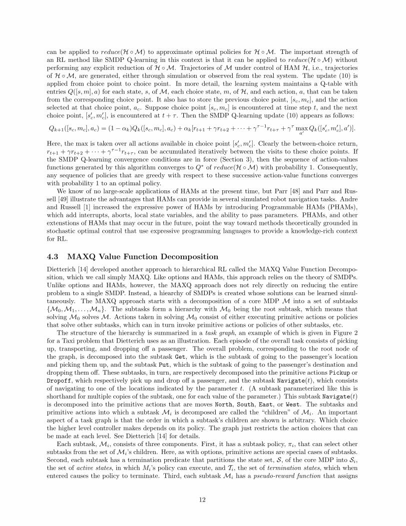
4.3 MAXQ Value Function Decomposition

Dietterich [14] developed another approach to hierarchical RL called the MAXQ Value Function Decompo-sition, which we call simply MAXQ. Like options and HAMs, this approach relies on the theory of SMDPs.Unlike options and HAMs, however, the MAXQ approach does not rely directly on reducing the entireproblem to a single SMDP. Instead, a hiearchy of SMDPs is created whose solutions can be learned simul-taneously. The MAXQ approach starts with a decomposition of a core MDP M into a set of subtasks{M0,M1, . . . ,Mn}. The subtasks form a hierarchy with M0 being the root subtask, which means thatsolving M0 solves M. Actions taken in solving M0 consist of either executing primitive actions or policiesthat solve other subtasks, which can in turn invoke primitive actions or policies of other subtasks, etc.

The structure of the hierarchy is summarized in a task graph, an example of which is given in Figure 2for a Taxi problem that Dietterich uses as an illustration. Each episode of the overall task consists of pickingup, transporting, and dropping off a passenger. The overall problem, corresponding to the root node ofthe graph, is decomposed into the subtask Get, which is the subtask of going to the passenger’s locationand picking them up, and the subtask Put, which is the subtask of going to the passenger’s destination anddropping them off. These subtasks, in turn, are respectively decomposed into the primitive actions Pickup orDropoff, which respectively pick up and drop off a passenger, and the subtask Navigate(t), which consistsof navigating to one of the locations indicated by the parameter t. (A subtask parameterized like this isshorthand for multiple copies of the subtask, one for each value of the parameter.) This subtask Navigate(t)is decomposed into the primitive actions that are moves North, South, East, or West. The subtasks andprimitive actions into which a subtask Mi is decomposed are called the “children” of Mi. An importantaspect of a task graph is that the order in which a subtask’s children are shown is arbitrary. Which choicethe higher level controller makes depends on its policy. The graph just restricts the action choices that canbe made at each level. See Dietterich [14] for details.

Each subtask, Mi, consists of three components. First, it has a subtask policy, πi, that can select othersubtasks from the set ofMi’s children. Here, as with options, primitive actions are special cases of subtasks.Second, each subtask has a termination predicate that partitions the state set, S, of the core MDP into Si,the set of active states, in which Mi’s policy can execute, and Ti, the set of termination states, which whenentered causes the policy to terminate. Third, each subtask Mi has a pseudo-reward function that assigns

12

Root

Get Put

Pickup Navigate(t) Dropoff

North South East West

Figure 2: A Task Graph for the Taxi Problem (after Dietterich [14]).

reward values to the states in Ti. The pseudo-reward function is only used during learning, which we discussafter first describing how the task graph hierarchy allows value functions to be decomposed.

A subtask is very much like a hierarchical option, 〈Ii, µi, βi〉, as defined in Section 4.1, with the additionof a pseudo-reward function. The policy over options, µi, corresponds to the subtask’s πi; the terminationcondition, βi, in this case assigns to states termination probabilities of only 1 or 0; and the option’s inputset Ii corresponds to Si. Unlike the option formalism, however, which treats semi-Markov options, MAXQexplicitly adds a component to each state that gives the current contents, K, of a pushdown stack containingthe names and parameter values of the hierarchy of calling subtasks, as in subroutine handling of ordinaryprogramming languages. At any time step, the top of the stack contains the name of the subtask currentlybeing executed. Thus, while a subtask’s policy is non-Markov with respect to the state set of the core MDP,it is Markov with respect to this augmented state set. As a consequence, each subtask policy has to assignactions to every combination, [s,K], of core state s and stack contents K.

Given a hierarchical decomposition ofM into n subtasks as given by a task graph, a hierarchical policy isdefined to be π = {π0, . . . , πn}, where πi is the policy ofMi. The hierarchical value function for π gives thevalue, i.e., the expected return, for each state-stack pair, [s,K], given that π is followed from s when the stackcontents are K. This value is denoted V π([s,K]). The “top level” value of a state s is V π([s, nil]), indicatingthat the stack is empty. This is the value of s under the flat policy induced by the hierarchy of subtaskcalls starting from the root of the hierarchy. The projected value function of hierarchical policy π on subtaskMi gives the expected return of each state s under the assumption that πi is executed until it terminates.This projected value is denoted V π(i, s). This is the same as the value function of the hierarchical optioncorresponding to Mi as defined in Section 4.1.

Given a hierarchical decomposition ofM and a hierarchical policy, π, each subtaskMi defines a discrete-time SMDP with state set is Si. Its actions are its child subtasks, Ma, and its transition probabilities,Pi(s

′, τ |s, a) (cf. Eqs. 6 and 7), are well-defined given the policies of the lower-level subtasks. A key obser-vation, which follows that of Singh [66, 67], is that this SMDP’s expected immediate reward, Ri(s, a), forexecuting action (subtask) a is the projected value of π on subtask Ma. That is, for all s ∈ Si and all childsubtasks Ma of Mi, Ri(s, a) = V π(s, a). To see why this is true, suppose the core MDP is in state s whensubtask Mi selects one of its child subtasks, Ma, for execution. Expanding Ma’s policy down to primitiveactions results in a flat policy that accumulates rewards according to the core MDP untilMa terminates ata state s′ ∈ Ta. The waiting time for s when this action is chosen is the execution time of Ma’s policy. Thereward accumulated during this waiting time is V π(s, a). Given this, one can write a Bellman equation forthe SMDP corresponding to subtask Mi:

V π(i, s) = V π(πi(s), s) +∑

s′,τ

Pπi (s′, τ |s, πi(s))γτV π(i, s′), (15)

13

where V π(i, s′) is the expected return for completing subtask Mi starting in state s′ (cf. Eq. 6).The action-value function, Q, defined by (1) can be extended to apply to subtasks: for hierarchical policy

π, Qπ(i, s, a) is the expected return for action a (a primitive action or a child subtask) being executed insubtask Mi and then π being followed until Mi terminates. In terms of this subtask action-value function,the observation expressed in (15) takes the form:

Qπ(i, s, a) = V π(a, s) +∑

s′,τ

Pπi (s′, τ |s, a)γτQπ(i, s′, π(s′)). (16)

Dietterich [14] calls the second term on the right of this equation the completion function:

Cπ(i, s, a) =∑

s′,τ

Pπi (s′, τ |s, a)γτQπ(i, s′, π(s′)).

This gives expected return for completing subtask Mi after subtask Ma terminates. Rewriting (16) usingthe completion function, we have

Qπ(i, s, a) = V π(a, s) + Cπ(i, s, a). (17)

Now it is possible to describe the MAXQ hierarchical value function decomposition. Given a hierarchicalpolicy π and a state s of the core MDP, suppose the policy of the top-level subtask, M0, selects subtaskMa1 , and that this subtask’s policy selects subtask Ma2 , whose policy in turn selects subtask Ma3 , etc.until finally subtask Man−1 ’s policy selects an, a primitive action that is executed in the core MDP. Thenthe projected value of s for the root subtask, V π(0, s), which is the value of s in the core MDP, can bewritten as follows:

V π(0, s) = V π(an, s) + Cπ(an−1, s, an) + · · ·+ Cπ(a1, s, a2) + Cπ(0, s, a1), (18)

where V π(an, s) =∑s′ P (s′|s, an)R(s′|s, an).

The decomposition (18) is the basis of a learning algorithm that is able to learn hierarchical policies fromsample trajectories. The details of this algorithm are somewhat complex and beyond the scope of this review,but we describe the basic idea. This algorithm is a recursively applied form of SMDP Q-learning that takesadvantage of the MAXQ value function decomposition to update estimates of subtask completion functions.The simplest version of this algorithm applies when the pseudo-reward functions of all the subtasks areidentically zero. The key component of the algorithm is a function—called MAXQ-0 for this special case—that calls itself recursively to descend through the hierarchy to finally execute primitive actions. When itreturns from each call, it updates the completion function corresponding to the appropriate subtask, withdiscounting determined by the returned count of the number of primitive actions executed. For details seeDietterich [14].

If the agent follows a policy that is GLIE (Section 3) and also further constrained to always break ties inthe same order, and the step-size parameter converges to zero according to the usual stochastic approximationconditions, then the algorithm sketched above converges with probability 1 to the unique recursively optimalpolicy for M that is consistent with the task graph. A recursively optimal policy is a hierarchical policy,π = {π0, . . . , πn}, such that for each subtask Mi, i = 0, . . . , n, πi is optimal for the SMDP correspondingto Mi, given the policies of Mi’s children subtasks. This form of optimal policy stands in contrast to ahierarchically optimal policy, which is a hierarchical policy that is optimal among all the policies that canbe expressed within the constraints imposed by the given hierarchical structure.

Examples of policies that are recursively optimal but not hierarchically optimal are easy to construct.This is because the hierarchical optimality of a subtask generally depends not only on that subtask’s children,but also on how the subtask participates in higher-level subtasks. For example, the hierarchically optimalway to travel to a given destination may depend on what you intend to do after arriving there in additionto properties of the trip itself. SMDP DP or RL methods applied to HAMs, or to MDPs with options whosepolicies are fixed a priori, yield hierarchically optimal policies, and it is relatively easy to define a learningalgorithm for MAXQ hierarchies that also produces hierarchically optimal policies. Dietterich’s interest inthe weaker recursive optimality stems from the fact that this form of optimality can be determined withoutconsidering the context of a subtask. This facilitates using subtask policies a building blocks for other tasksand has implications for state abstraction, although we do not touch on the latter aspect in this review.

14

What about the pseudo-reward functions? These functions allow a system designer within the MAXQframework to specify subtasks by defining subgoals that they must achieve but without specifying policiesfor achieving them. In this respect, they play the same role as do the auxiliary reward functions that canbe used in the options framework for learning option policies. The MAXQ-0 learning algorithm sketchedabove can be extended to an algorithm, called MAXQ-Q, that learns a policy that is recursively optimalhierarchical with respect to the sum of the original reward function and the pseudo-reward functions.

We have not been able to do justice to the MAXQ approach and associated algorithms in this shortreview. However, we have presented enough to provide a basis for seeing how SMDP theory again plays acentral role in an approach to hierarical RL. Like HAMs, MAXQ is an excellent example of how conceptsfrom programming languages can be fruitfully integrated with a stochastic optimal control framework.

5 Recent Advances in Hierarchical RL

Thus far we have surveyed different approaches to hierarchical RL, all of which are based on the underlyingframework of SMDPs. These approaches collectively suffer from some key limitations: policies are restrictedto sequential combinations of activities; agents are assumed to act alone in the environment; and finally,states are considered to be fully accessible. In this section, we address these assumptions and describe howthe SMDP framework can be extended to concurrent activities, multiagent domains, and partially observablestates.

5.1 Concurrent Activities

Here we summarize recent work by Rohanimanesh and Mahadevan [57] towards a general framework formodeling concurrent activities. This framework is motivated by situations in which a single agent canexecute multiple parallel processes, as well as by the multiagent case in which many agents act in parallel(addressed in Section 5.2). Managing concurrent activities clearly is a central component of our everydaybehavior: in making breakfast, we interleave making toast and coffee with other activities such as gettingmilk; in driving, we search for road signs while controlling the wheel, accelerator and brakes.

Building on the SMDP framework described above, this approach focuses on modeling concurrent activi-ties, where each component activity is temporally extended. One immediate question that arises in modelingconcurrent activities is that of termination: unlike the purely sequential case, when multiple activities areexecuted simultaneously, concurrently executing activities do not generally terminate at the same time. Howdoes one define the termination of a set of concurrent activities? Among the termination schemes studiedby Rohanimanesh and Mahadevan [57] are the following two. The any scheme terminates all other activitieswhen the first activity terminates, whereas the all scheme waits until all existing activities terminate beforechoosing a new concurrent set of activities. These researchers have also studied other schemes, such as con-tinue, which replaces the terminated activity with a set of new activities that includes the activities alreadyexecuting. For simplicity, we restrict our discussion to the first two schemes.

For concreteness, we describe the concurrent activity model using the options formalism described inSection 4.1. The treatment here is restricted to options over discrete-time SMDPs and having deterministicpolicies, but the main ideas extend readily to the other variants (HAMs, MAXQ), as well as to continuous-time SMDPs. (See ref. [21] for a treatment of hierarchical RL for continuous-time SMDPs.) The sequentialoption model is generalised to a multi-option, which is a set of options that can be executed in parallel.Here we discuss the simple case in which the options comprising a multi-option influence different sets ofstate variables that do not interact. (This assumption can be generalized, but for simplicity, we restrict ourtreatment here.) For example, turning the radio off and pressing the brake can always be executed in parallelsince they affect different non-interacting state variables.

We now define a multi-option (denoted by ~o) more precisely. Let o =< I, π, β > be an option as definedin Section 4.1 on a core MDP with state set S ⊆ Πn

1Si, where Si is the range of state variable si, i = 1, . . . , n.Suppose that while option o is executing, it influences only a subset of the state variables So ⊆ {s1, s2, ..., sn}.Assume also that while o is executing, these variables do not influence, and are not influenced by, any variablesnot in So. A set of options {o1, . . . , om}, each defined on the same core MDP, is coherent if ∩m1 Soi = ∅.This ensures that each option will affect different components of the state set so that any subset of themcan be executed in parallel without interfering with one another. In other words, while a coherent set of

15

options is executing, the system admits a parallel decomposition with each component corresponding to thestate variables influenced by one of the options. In the driving example, the turn-radio-on and brake

options comprise a coherent set, but the turn-right and accelerate options do not since the state variableposition is influenced by both. A multi-option over an MDP M is a coherent set of options over M.

When multi-option ~o is executed in state s, several options oi ∈ ~o are initiated. Each option oi willterminate at some random time toi . We can define the termination of a multi-option based on either of thefollowing events: (1) Tall = maxi(toi): when all the options oi ∈ ~o terminate according to βi(s), multi-option~o is declared terminated, or (2) Tany = mini(toi): when any (i.e., the first) of the options terminate, theoptions that are still executing at that time are interrupted.

We then have the following result. Given a finite MDP and a collection of multi-options defined on it,where the underlying options are Markov, the decision process that selects only among multi-options, andexecutes each one until its termination according to the Tall or Tany termination conditions, is a discrete-timeSMDP. The proof requires showing that the state transition probabilities and the rewards corresponding toany concurrent option ~o defines an SMDP [57]. The significance of this result is that SMDP Q-learningmethods can be extended to learn policies over concurrent options under this model.

The extended SMDP Q-learning algorithm for learning policies over multi-options updates the multi-option value function Q(s, ~o) after each decision epoch in which the multi-option ~o is taken in state s andterminates in state s′ (under either termination condition):

Qk+1(s, ~o) = (1− αk)Qk(s, ~o) + α

[r + γτ max

~o′∈Os′Qk(s′, ~o′)

], (19)

where τ denotes the number of time steps between initiation of the multi-option ~o in state s and its ter-mination in state s′, and r denotes the cumulative discounted reward over this period. This learning rulegeneralizes (13) to multi-options. It is straightforward to also generalize other learning algorithms, such asthe intra-option Q-learning algorithm (14) to multi-options.

As a simple illustrative example of using this concurrent SMDP Q-learning algorithm, Rohanimaneshand Mahadevan [57] considered an environment consisting of four “rooms”, each of which is divided into adiscrete set of cells (Figure 3). Each room contains two doors, each of which can be “opened” by two keys.The agent is given options for getting to each door from any interior room state, and for opening a lockeddoor. It has to learn the shortest path to the goal by concurrently combining these options. The agent canreach the goal more quickly if it learns to parallelize the option for retrieving the key before it reaches alocked door. However, retrieving the key too early is counterproductive since it can be dropped with someprobability. The process of retrieving a key is modeled as an SMDP consisting of a linear chain of states tomodel the waiting process before the agent is holding the key.

Figure 4 compares the policies learned with strictly sequential options, as described in Section 4.1, usingthe Q-learning algorithm (13), with policies over multi-options learned using the extended Q-learning rule(19). The vertical axis plots the median steps to the goal in each trial. Note that the sequential solution isthe slowest, taking the agent about 50 steps to reach the goal. The termination condition Tall is faster thanthe sequential case, taking about 45 steps to reach the goal. Both of these, however, are significantly slowerthan the Tany and Tcontinue policies, which reach the goal in half the time. Tany converges the slowest, sinceit terminates multi-options fairly aggressively resulting in more decision epochs. Tcontinue provides the besttradeoff between speed of convergence and optimality of the learned policy.

The multi-option formalism can be extended to allow cases in which options executing in parallel modifythe same shared variables at the same time. Details of this extension is beyond the scope of the presentarticle.

5.2 Multiagent Coordination

Concurrency is the basis for modeling coordination among multiple simultaneously behaving agents. Froma theoretical point of view, it matters little if concurrent activities are being executed by a single agent orby multiple cooperating agents. However, the multiagent problem usually involves other complexities aswell, such as the fact that one agent cannot usually observe the actions or the states of other agents in theenvironment. We address the issue of hidden state in the next section; here we focus on the problem oflearning a policy across joint states and joint actions.

16

(to each room’s 2 hallways)- One single step no-op option

- 8 multi-step navigation options

- 3 stochastic primitive actions for keys(get-key, key-nop and putback-key)

each key- Drops the keys 20% of times when passingthrough the water trap and holding both keys

- 2 multi-step key options (pickup-key) for

water trap

and holding both keys

- 4 stochastic primitive actions(Up, Down, Left and Right)- Fail 10% of times, when not passingthe water trap- Fail 30% of times, when passing thewater trap

Agent H0

H2

H1 H3 (Goal)

Figure 3: An Illustrative Problem for Concurrent Options.

20

25

30

35

40

45

50

55

60

65

70

0 100000 200000 300000 400000 500000

Med

ian/

Tria

ls (

step

s to

goa

l)

Trial

Sequential OptionsConcurrent Options: optimal, T-all

Concurrent Options: optimal, T-anyConcurrent Options: continue

Figure 4: Multi-Option Comparison. This graph compares a multi-option SMDP Q-learning system (underdifferent termination schemes) with one that learns sequential policies. Policies over multi-options easilyoutperform sequential policies, and termination makes a large difference in of convergence rate and qualityof the learned policy.

In general, problems involving multiagent coordination can be modeled by assuming that states nowrepresent the joint state of n agents, where each agent i may only have access to a partial view si. Also,the joint action is represented as (a1, . . . , an), where again, each agent may not have knowledge of the otheragents’ actions. Typically, the assumption made in multiagent studies is that the set of joint actions definesan SMDP (or MDP) over the joint state set. Of course, in most practical problems, the joint state andaction sets are exponential in the number of agents, and the aim is to find a distributed solution that does

17

not require combinatorial enumeration over joint states and actions.One general approach to learning task-level coordination is to extend the above concurrency model to

the joint state and action spaces, where each action is a fixed option with a pre-specified policy. Thisapproach requires very minimal modification of the approach described in the previous section. In contrast,we now describe an extension of this approach due to Makar and Mahadevan [41] in which agents learnboth coordination skills and the base-level policies using a multiagent MAXQ-like task graph. However,convergence to (hierarchically) optimal policies is no longer assured since lower-level subtask policies arevarying at the same time when learning higher-level politices. The ideas can be extended to other formalismsalso, but for the sake of clarity, we focus on the MAXQ value function decomposition approach described inSection 4.3.

It is necessary to generalize the MAXQ decomposition from its original sequential single-agent settingto the multiagent coordination problem. Let ~o = (o1, ..., on) denote a multi-option, where oi is the optionexecuted by agent i.3 Let s = (s1, ..., sn) denote a joint state. The joint action-value of a multi-option ~o in ajoint state s, and in the context of doing parent task p, is denoted Q(p, s, ~o). The MAXQ decomposition ofthe Q-function given by (17) can be extended to joint action-values as follows. The joint completion functionfor agent j assigns values Cj(p, sj , ~o) giving the discounted return for agent j completing a multi-optionin in the context of doing parent task p, when the other agents are performing multi-options ok, for allk ∈ {1, . . . , n}, k 6= j. The joint mulit-option value Q(p,~s, ~o) is now approximated by each agent j (givenonly its local state sj) as:

Qj(p, sj , ~o) ≈ V j(~oj , sj) + Cj(p, sj , ~o),

where

V j(p, sj) =

{max ~ok Q

j(p, sj , ~ok) if parent task p is non-primitive∑s′jP (s′j | sj , p)R(s′j | sj , p) if p is a primitive action.

The first term in the Q(p, sj , ~o) expansion above refers to the discounted sum of rewards received by agent jfor doing concurrent action ~oj in state sj . The second term “completes” the sum by accounting for rewardsearned for completing the parent task p after finishing ~oj . The completion function is updated from samplevalues using an SMDP learning rule. Note that the correct action value is approximated by only consideringlocal state sj and also by ignoring the effect of concurrent actions ~ok, k 6= j by other agents when agent j isperforming ~oj . In practice, a human designer can configure the task graph to store joint concurrent actionvalues at the highest level(s) of the hierarchy as needed.

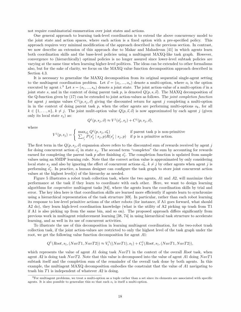
Figure 5 illustrates a robot trash collection task, where the two agents, A1 and A2, will maximize theirperformance at the task if they learn to coordinate with each other. Here, we want to design learningalgorithms for cooperative multiagent tasks [84], where the agents learn the coordination skills by trial anderror. The key idea here is that coordination skills are learned more efficiently if agents learn to synchronizeusing a hierarchical representation of the task structure [69]. In particular, rather than each robot learningits response to low-level primitive actions of the other robots (for instance, if A1 goes forward, what shouldA2 do), they learn high-level coordination knowledge (what is the utility of A2 picking up trash from T1if A1 is also picking up from the same bin, and so on). The proposed approach differs significantly fromprevious work in multiagent reinforcement learning [38, 74] in using hierarchical task structure to acceleratelearning, and as well in its use of concurrent activities.

To illustrate the use of this decomposition in learning multiagent coordination, for the two-robot trashcollection task, if the joint action-values are restricted to only the highest level of the task graph under theroot, we get the following value function decomposition for agent A1:

Q1(Root, s1, (NavT1, NavT2)) ≈ V 1t ((NavT1), s1) + C1

t (Root, s1, (NavT1, NavT2)),

which represents the value of agent A1 doing task NavT1 in the context of the overall Root task, whenagent A2 is doing task NavT2. Note that this value is decomposed into the value of agent A1 doing NavT1subtask itself and the completion sum of the remainder of the overall task done by both agents. In thisexample, the multiagent MAXQ decomposition embodies the constraint that the value of A1 navigating totrash bin T1 is independent of whatever A2 is doing.

3For multiagent problems, we treat a multi-option as a tuple rather than a set since its elements are associated with specificagents. It is also possible to generalize this so that each oi is itself a multi-option.

18

Dump

Room1

Room2

Room3

T2

T2: Location of another trash can.

T1: Location of one trash can.

Corridor

T1

A2

A1

Dump: Final destination location for depositing all trash.

Root

Max Node

Q Node

:

:

PickPut

PutNav

Follow Align Find

Follow Find

NavDNavT2NavT1

T2: Location of Trash 2

T1: Location of trash 1

D: Location of dump

Pick

Align

Figure 5: A Two-Robot (A1 and A2) Trash Collection Task. The robots can learn to coordinate much morerapidly using the task structure than if they attempted to coordinate at the level of primitive movements.On the right is shown a MAXQ graph, which is MAXQ task graph with two kinds of nodes representingsubtasks and the actions those subtasks can select [14].

5.3 Hierarchical Memory

In multiagent environments, agents cannot observe joint states and joint actions, but must act based onestimates of these hidden variables (the problem of hidden state occurs in many single-agent tasks as well,such as a robot navigating in an indoor office environment). One approach is formalized in terms of Partiallyobservable Markov decision processes (POMDPs), where agents learn policies over belief states, i.e., proba-bility distributions over the underlying state set [31]. It can be shown that belief states satisfy the Markovproperty and consequently yield a new (and more complex) MDP over information states. Belief statescan be recursively updated using the transition model, and an observation model O(y | s, a) specifying thelikelihood of observing y if action a was performed and resulted in state s. However, mapping belief statesto optimal actions is known to be intractable, particularly in the decentralized multiagent formulation [3].Also, learning a perfect model of the underlying POMDP is a challenging task. An empirically more effective(but theoretically less powerful) approach is to use finite memory models as linear chains or nonlinear treesover histories [42]. However, such finite memory structures can be defeated by long sequences of mostlyirrelevant observations and actions that conceal a critical past observation.

We briefly summarize three multiscale memory models that have been explored recently by Hernandezand Mahadevan [25], Theocharous and Mahadevan [79], and Jonsson and Barto [30]. These models combinetemporal abstraction with previous methods for dealing with hidden state. Hierarchical Suffix Memory(HSM) [25] generalizes the suffix tree model [42], to SMDP-based temporally-extended activities. Suffixmemory constructs state estimators from finite chains of observation-action-reward triples. In additionto extending suffix models to temporally-extended activities, HSM also uses multiple layers of temporalabstraction to form longer-term memories at more abstract levels. Figure 6 illustrates this idea for robotnavigation for the simpler case of a linear chain, although the tree-based model has also been investigated.An important side-effect is that the agent can look back many steps back in time while ignoring the exactsequence of low-level observations and actions that transpired. Tests in a robot navigation domain showedthat HSM outperformed “flat” suffix tree methods, as well as hierarchical methods that used no memory[25].

POMDPs are theoretically more powerful than finite memory models, but past work on POMDPs hasmostly studied “flat” models for which learning and planning algorithms scale poorly with model size.Theocharous et al. [79] developed a hierarchical POMDP formalism, termed H-POMDPs (Figure 7), byextending the hierarchical hidden Markov model (HHMM) [19] to include rewards and temporally-extended

19

. . .. . . . . .

*?

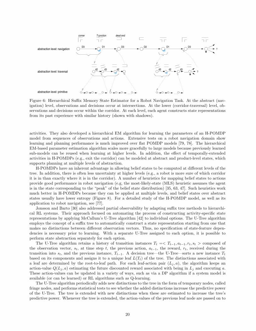
T-junctioncorner dead end

D3 D1 D3 D2 D1 D3

*. . . ?

d3 d2 d3d3 d2d2

abstraction level: navigation

abstraction level: traversal

abstraction level: primitive

Figure 6: Hierarchical Suffix Memory State Estimator for a Robot Navigation Task. At the abstract (nav-igation) level, observations and decisions occur at intersections. At the lower (corridor-traversal) level, ob-servations and decisions occur within the corridor. At each level, each agent constructs state representationsfrom its past experience with similar history (shown with shadows).

activities. They also developed a hierarchical EM algorithm for learning the parameters of an H-POMDPmodel from sequences of observations and actions. Extensive tests on a robot navigation domain showlearning and planning performance is much improved over flat POMDP models [79, 78]. The hierarchicalEM-based parameter estimation algorithm scales more gracefully to large models because previously learnedsub-models can be reused when learning at higher levels. In addition, the effect of temporally-extendedactivities in H-POMDPs (e.g., exit the corridor) can be modeled at abstract and product-level states, whichsupports planning at multiple levels of abstraction.

H-POMDPs have an inherent advantage in allowing belief states to be computed at different levels of thetree. In addition, there is often less uncertainty at higher levels (e.g., a robot is more sure of which corridorit is in than exactly where it is in the corridor). A number of heuristics for mapping belief states to actionsprovide good performance in robot navigation (e.g, the most-likely-state (MLS) heuristic assumes the agentis in the state corresponding to the “peak” of the belief state distribution) [35, 63, 47]. Such heuristics workmuch better in H-POMDPs because they can be applied at multiple levels, and belief states over abstractstates usually have lower entropy (Figure 8). For a detailed study of the H-POMDP model, as well as itsapplication to robot navigation, see [77].

Jonsson and Barto [30] also addressed partial observability by adapting suffix tree methods to hierarchi-cal RL systems. Their approach focused on automating the process of constructing activity-specific staterepresentations by applying McCallum’s U-Tree algorithm [42] to individual options. The U-Tree algorithmemploys the concept of a suffix tree to automatically construct a state representation starting from one thatmakes no distinctions between different observation vectors. Thus, no specification of state-feature depen-dencies is necessary prior to learning. With a separate U-Tree assigned to each option, it is possible toperform state abstraction separately for each option.

The U-Tree algorithm retains a history of transition instances Tt =< Tt−1, at−1, rt, st > composed ofthe observation vector, st, at time step t, the previous action, at−1, the reward, rt, received during thetransition into st, and the previous instance, Tt−1. A decision tree—the U-Tree—sorts a new instance Ttbased on its components and assigns it to a unique leaf L(Tt) of the tree. The distinctions associated witha leaf are determined by the root-to-leaf path. For each leaf-action pair (Lj , a), the algorithm keeps anaction-value Q(Lj , a) estimating the future discounted reward associated with being in Lj and executing a.These action-values can be updated in a variety of ways, such as via a DP algorithm if a system model isavailable (or can be learned) or RL algorithms such as Q-learning.

The U-Tree algorithm periodically adds new distinctions to the tree in the form of temporary nodes, calledfringe nodes, and performs statistical tests to see whether the added distinctions increase the predictive powerof the U-Tree. The tree is extended with new distinctions when these are estimated to increase the tree’spredictive power. Whenever the tree is extended, the action-values of the previous leaf node are passed on to

20

en en en en

1.0 1.0 1.0 1.0

0.9 0.9

0.1 0.1 0.1 0.1

0.9

0.9

0.90.10.10.10.10.1

0.9 0.9

0.90.9

0.9

0.9

0.1

1.01.0

0.1

s 0

ex ex ex3

s 4

s 1 s 2

s 5s 6

ex8

s

7

9 s 10

11

0.1

0.9

0.25 0.25 0.250.25

Figure 7: Hierarchical POMDP Model. This hierarchical POMDP model represents two adjacent corridorsin a robot navigation task. The model has two primitive actions, “go-left” indicated with the dotted arrowsand “go-right” indicated with the dashed arrows. This HPOMDP has two (unobservable) abstract states s1

and s2, and each abstract state has two entry and two exit states. The (hidden) product states s4, s5, s6,s9, and s10 have associated observation models.

0

0.2

0.4

0.6

0.8

1

0 10 20 30 40 50 60 70 80 90 100

Nor

mal

ized

ent

ropi

es

Number of steps

Normalized entropies of the abstract and global levels

Global entropyAbstract entropy

START

GOAL

2J

J4

J3

J1

Figure 8: Entropy of a Sample Robot Navigation Run. This graph shows a sample robot navigation runwhose trace is on the right, where positional uncertainty (measured by belief state entropy) at the abstract(corridor) level is less than at the product state level. Spatiotemporal abstraction reduces the uncertainty andrequires less frequent decision-making, allowing the robot to get to goals without inital positional information.

the new leaf nodes. Each distinction is based on (1) a perceptual dimension, which is either an observationor a previous action, and (2) a history index, indicating how far back in the current history the dimensionwill be examined.

Jonsson and Barto [30] adapted the U-Tree algorithm for use with options and hierarchical learningarchitectures. Given a finite MDP and a set of options whose policies were not yet defined, they assignedeach option a separate U-Tree, which was updated using the U-Tree algorithm (with some modifications)based on each option’s local history. What makes the U-Tree algorithm suitable for performing option-specific state abstraction is that a U-Tree simultaneously defines a state representation and a policy over this

21

representation. By assigning one U-Tree to each option, the algorithm is able to perform state abstractionseparately for each option while also modifying its policy. It is also possible to use intra-option learningmethods (Section 4.1) so that something about an option can be learned from the behavior of other options.

This version of the U-Tree algorithm was illustrated using Dietterich’s [14] Taxi task that we briefly de-scribed in Section 4.3. Results show that starting with no distinctions being made in the state representation(i.e., all states were represented as a single block), the algorithm was able to solve this task by introducingdistinctions that partitioned the state-action set into subsets requiring different action-values, at a significantsavings over an approach that initially distinguished between all possible states. Although this example ismerely illustrative, it suggests that automated option-specific state abstraction is an attractive approach tomaking hierarchical learning systems more powerful.

6 Topics For Future Research

6.1 Compact Representations

In most interesting real-world tasks, states have significant internal structure. For example, states are veryoften represented as vectors of state variables (usually called factored states by machine learning researchers),or even possess richer relational structure [17]. Much work in artificial intelligence has focused on exploit-ing this structure to develop compact representations of single-step actions (e.g., the Dynamic Bayes Netrepresentation [13]). A natural question to consider is how to extend these single-step compact models intocompact models of temporally-extended activities, such as options. The problem is a bit subtle since evenif all actions have limited single-step influence on state variables, this property generally does not hold overan extended activity. One approach that Rohanimanesh and Mahadevan [56] have been studying is how toexploit results from approximation of structured stochastic processes [6] to develop structured ways of ap-proximating the next-state predictions of temporally-extended activities. The key idea is that by clusteringthe state variables into disjoint subsets, and keeping track of a next-state distribution for each local clus-ter, it is possible to efficiently approximate the underlying next-state distribution for a temporally-extendedactivity. Preliminary analysis of this approach appears promising, and further theoretical and experimentalstudy is under way.

6.2 Learning Task Hierarchies

In the approaches discussed above, the components of the hierarchy, their places in the hierarchy, and theabstractions that are used are decided upon in advance. A key open question is how to form task hierarchiesautomatically, such as those used in the MAXQ framework. We briefly discussed in Section 4.1 automatedmethods for identifying useful subtoals [15, 16, 43, 44] which address some aspects of this problem. Anotherapproach called HEXQ was recently proposed by Hengst [24]. It exploits a factored state representationand sorts state variables into an ordered list, beginning with the variable that changes most rapidly. HEXQbuilds a task hierarchy, consisting of one level for each state variable, where each level contains a simplerMDP that is connected to other smaller MDPs through a set of “bottleneck” states (for example, if theenvironment is a set of rooms, as in the navigation example shown in Figure 3 above, each room wouldcorresond to such a smaller MDP). The obvious limitation of HEXQ is that it is limited to considering eachstate variable in isolation, an approach that fails for more complex problems. Further work is required forunderstanding how to build task hierarchies in such cases, and how to integrate this approach to relatedsystems approaches such as singular perturbation methods [36, 46].

6.3 Dynamic Abstraction

Systems such as those outlined in this article naturally provide opportunities for using different state rep-resentations depending on the activity that is currently executing. There is a crucial distinction betweenstatic abstractions, which remain fixed throughout all phases of a sequential decision task, and what we calldynamic abstractions that are conditional on the execution of particular temporally-extended activities. Inother words, the variables that a dynamic abstraction renders relevant or irrelevant are afforded that statusonly for a temporally-confined segment of time. For example, during the course of driving, the steering wheel

22

angle, the gear position, or the radio status may all be relevant, but become irrelevant during other activi-ties. Dietterich [14] introduced activity-specific state abstraction in the MAXQ framework, and Jonsson andBarto [30] explored automatic methods for constructing such representation from experience, as describedin Section 5.3. The ability to use dynamic abstraction in RL is one of the key reasons that the hierarchicalRL approaches discussed in this article appear so attractive to machine learning researchers. This is an areain which future research can have a significant impact.

6.4 Large Applications

Although the proposed ideas for hierarchical RL described above appear promising, to date there has beeninsufficient experience in experimentally testing the effectiveness of these ideas on large applications. Makar,Mahadevan, and Ghavamzadeh [41] extended the MAXQ approach to multiagent domains, and applied itto a large multi-vehicle autonomous guided vehicle (AGV) routing problem. They demonstrated that thepolicies learned for this problem were better than standard heuristics used in industry, such as the “go tothe nearest free machine” heuristic. Stone and Sutton [68] applied the framework of options to a “keepaway” task in Robot soccer. This task involves a set of players from one team passing the ball betweenthem and keeping the ball in their possession against the defending opponents. While these initial studiesare promising, much further work is necessary to establish the effectiveness of hierarchical RL, particularlyon large complex continuous control tasks.

7 Conclusion

It has been our goal in the article to review several closely related approaches to temporal abstraction andhierarchical control that have been developed by machine learning researchers: the options formalism ofSutton, Precup, and Singh, the hierarchies of abstract machines (HAMs) approach of Parr and Russell,and Dietterich’s MAXQ framework. We also discussed extensions of these ideas addressing on concurrentactivities, multiagent coordination, and hierarchical memory for partial observability. Although many ofthese ideas are closely related to similar concepts in systems and control engineering on hierarchical, hybrid,and multilayer control, we have not attempted to provide a careful rapprochement between these areas andwhat machine learning, and other researchers associated with artificial intelligence, have been developing.However, we strongly believe that there is much to be gained—on both sides—from such a rapproachement,and it is our hope that this article will prove to be useful in stimulating the needed dialog.

AcknowledgmentsThe authors would like to thank Anders Jonsson, Khashayar Rohanimanesh, and Mohammad Ghavamzadeh for their

crtical reading of an early draft of this article. This work was funded by the National Science Foundation under

Grant No. ECS-9980062. Any opinions, findings, and conclusions or recommendations expressed in this material are

those of the authors and do not necessarily reflect the views of the National Science Foundation.

References

[1] D. Andre and S. J. Russell. Programmable reinforcement learning agents. In Advances in NeuralInformation Processing Systems: Proceedings of the 2000 Conference, pages 1019–1025, Cambridge,MA, 2001. MIT Press.

[2] A. G. Barto, S. J. Bradtke, and S. P. Singh. Learning to act using real-time dynamic programming.Artificial Intelligence, 72:81–138, 1995.

[3] D. Bernstein, S. Zilberstein, and N. Immerman. The complexity of decentralized control of markovdecision processes. In 16th Conference on Uncertainty in Artificial Intelligence, 2000.

[4] D. P. Bertsekas. Dynamic Programming: Deterministic and Stochastic Models. Prentice-Hall, EnglewoodCliffs, NJ, 1987.

23

[5] D. P. Bertsekas and J. N. Tsitsiklis. Neuro-Dynamic Programming. Athena Scientific, Belmont, MA,1996.

[6] X. Boyen and D. Koller. Tractable inference for complex stochastic processes. In G. F. Cooper andS. Moral, editors, Proceedings of the Fourteenth Conference on Uncertainty in AI, pages 33–42, SanFrancisco, CA, 1998. Morgan Kaufmann.

[7] S. J. Bradtke and M. O. Duff. Reinforcement learning methods for continuous-time markov decisionproblems. In G. Tesauro, D. S. Touretzky, and T. Leen, editors, Advances in Neural InformationProcessing Systems: Proceedings of the 1994 Conference, pages 393–400, Cambridge, MA, 1995. MITPress.

[8] M. S. Branicky, V. S. Borkar, and S. K. Mitter. A unified framework for hybrid control: Model andoptimal control theory. IEEE Transactions on Automatic Control, 43:31=45, 1998.

[9] R. A. Brooks. Achieving artificial intelligence through building robots. Technical Report A.I. Memo899, Massachusetts Institute of Technology Artificial Intelligence Laboratory, Cambridge, MA, 1986.

[10] R. H. Crites. Large-Scale Dynamic Optimization Using Teams of Reinforcement Learning Agents. PhDthesis, University of Massachusetts, Amherst, MA, 1996.

[11] R. H. Crites and A. G. Barto. Elevator group control using multiple reinforcement learning agents.Machine Learning, 33:235–262, 1998.

[12] T. K. Das, A. Gosavi, S. Mahadevan, and N. Marchalleck. Solving semi-markov decision problems usingaverage reward reinforcement learning. Management Science, 45:560–574, 1999.

[13] T. L. Dean and K. Kanazawa. A model for reasoning about persistence and causation. ComputationalIntelligence, 5:142–150, 1989.

[14] T. G. Dietterich. Hierarchical reinforcement learning with the maxq value function decomposition.Journal of Artificial Intelligence Research, 13:227–303, 2000.

[15] B. Digney. Emergent hierarchical control structures: Learning reactive/hierarchical relationships inreinforcement environments. In P. Meas and M. Mataric, editors, From Animals to Animats 4: TheFourth Conference on Simulation of Adaptive Behavior. MIT Press, 1996.

[16] B. Digney. Learning hierarchical control structure from multiple tasks and changing environments. InFrom Animals to Animats 5: The Fifth Conference on Simulation of Adaptive Behavior. MIT Press,1998.

[17] K. Driessens and S. Dzeroski. Integrating experimentation and guidance in relational reinforcementlearning. In Maching Learning: Proceedings of the Nineteenth International Conference on MachineLearning, 2002.

[18] R. E. Fikes, P. E. Hart, and N. J. Nilsson. Learning and executing generalized robot plans. ArtificialIntelligence, 3:251–288, 1972.

[19] S. Fine, Y. Singer, and N. Tishby. The Hierarchical Hidden Markov Model: Analysis and Applications.Machine Learning, 32(1), July 1998.

[20] J.-P. Forestier and P. Varaiya. Multilayer control of large markov chains. IEEE Transactions onAutomatic Control, AC-23:298–304, 1978.

[21] M. Ghavamzadeh and S. Mahadevan. Continuous-time hierarchical reinforcement learning. In Proceed-ings of the Eighteenth International Conference on Machine Learning, 2001.

[22] G. Z. Grudic and L. H. Ungar. Localizing search in reinforcement learning. In Proceedings of the 18thNational Conference on Artificial Intelligence, (AAAI-00), pages 590–595, 2000.

24

[23] D. Harel. Statecharts: A visual formalixm for complex systems. Science of Computer Programming,8:231–274, 1987.

[24] B. Hengst. Discovering hierarchy in reinforcement learning with hexq. In Maching Learning: Proceedingsof the Nineteenth International Conference on Machine Learning, 2002.

[25] N. Hernandez and S. Mahadevan. Hierarchical memory-based reinforcement learning. Proceedings ofNeural Information Processing Systems, 2001.

[26] R. A. Howard. Dynamic Probabilistic Systems: Semi-Markov and Decision Processes. Wiley, NY, 1971.

[27] M. Huber and R. A. Grupen. A feedback control structure for on-line learning tasks. Robotics andAutonomous Systems, 22:303–315, 1997.

[28] G. A. Iba. A heuristic approach to the discovery of macro-operators. Machine Learning, 3:285–317,1989.

[29] T. Jaakkola, M. I. Jordan, and S. P. Singh. On the convergence of stochastic iterative dynamic pro-gramming algorithms. Neural Computation, 6:1185–1201, 1994.

[30] A. Jonsson and A. G. Barto. Automated state abstraction for options using the U-tree algorithm.In Advances in Neural Information Processing Systems: Proceedings of the 2000 Conference, pages1054–1060, Cambridge, MA, 2001. MIT Press.

[31] L. Kaelbling, M. Littman, and A. Cassandra. Planning and acting in partially observable stochasticdomains. Artificial Intelligence, 101, 1998.

[32] L. P. Kaelbling, M. L. Littman, and A. W. Moore. Reinforcement learning: A survey. Journal ofArtificial Intelligence Research, 4:237–285, 1996.

[33] A. H. Klopf. Brain function and adaptive systems—A heterostatic theory. Technical Report AFCRL-72-0164, Air Force Cambridge Research Laboratories, Bedford, MA, 1972. A summary appears inProceedings of the International Conference on Systems, Man, and Cybernetics, 1974, IEEE Systems,Man, and Cybernetics Society, Dallas, TX.

[34] A. H. Klopf. The Hedonistic Neuron: A Theory of Memory, Learning, and Intelligence. Hemisphere,Washington, D.C., 1982.

[35] S. Koenig and R. Simmons. Xavier: A robot navigation architecture based on partially observablemarkov decision process models. In D. Kortenkamp, P. Bonasso, and Murphy. R., editors, AI-basedMobile Robots: Case-studies of Successful Robot Systems. MIT Press, 1997.

[36] P. V. Kokotovic, H. K. Khalil, and J. O’Reilly. Singular Perturbation Methods in Control: Analysis andDesign. Academic Press, London, 1986.

[37] R. E. Korf. Learning to Solve Problems by Searching for Macro-Operators. Pitman, Boston, MA, 1985.

[38] M. Littman. Markov games as a framework for multi-agent reinforcement learning. In Proceedings ofthe Eleventh International Conference on Machine Learning, pages 157–163, 1994.

[39] S. Mahadevan. Average reward reinforcement learning: Foundations, algorithms, and empirical results.Machine Learning, 22:159–196, 1996.

[40] S. Mahadevan, N. Marchalleck, T. Das, and A. Gosavi. Self-improving factory simulation usingcontinuous-time average-reward reinforcement learning. In Machine Learning: Proceedings of the Four-teenth International Conference, 1997.

[41] R. Makar, S. Mahadevan, and M. Ghavamzadeh. Hierarchical multi-agent reinforcement learning. InJ. P. Muller, E. Andre, S. Sen, and C. Frasson, editors, Proceedings of the Fifth International Conferenceon Autonomous Agents, pages 246–253, 2001.

25

[42] A. K. McCallum. Reinforcement Learning with Selective Perceptioin and Hidden State. PhD thesis,University of Rochester, 1996.

[43] A. McGovern. Autonomous Discovery of Temporal Abstractions from Interaction with An Environment.PhD thesis, University of Massachusetts, 2002.

[44] A. McGovern and A. Barto. Automatic discovery of subgoals in reinforcement learning using diversedensity. In C. Brodley and A. Danyluk, editors, Proceedings of the Eighteenth International Conferenceon Machine Learning, pages 361–368, San Francisco, CA, 2001. Morgan Kaufmann.

[45] M. L. Minsky. Theory of Neural-Analog Reinforcement Systems and its Application to the Brain-ModelProblem. PhD thesis, Princeton University, 1954.

[46] D. S. Naidu. Singular Perturbation Methodology in Control Systems. Peter Peregrinus Ltd., London,1988.

[47] I. Nourbakhsh, R. Powers, and S. Birchfield. Dervish: An office-navigation robot. AI Magazine,16(2):53–60, 1995.

[48] R. Parr. Hierarchical Control and Learning for Markov Decision Processes. PhD thesis, University ofCalifornia, Berkeley, CA, 1998.

[49] R. Parr and S. Russell. Reinforcement learning with hierarchies of machines. In Advances in NeuralInformation Processing Systems: Proceedings of the 1997 Conference, Cambridge, MA, 1998. MIT Press.

[50] T. J. Perkins and A. G. Barto. Lyapunov design for safe reinforcement learning. Journal of MachineLearning Research. To appear.

[51] T. J. Perkins and A. G. Barto. Lyapunov-constrained action sets for reinforcement learning. In C. Brod-ley and A. Danyluk, editors, Proceedings of the Eighteenth International Conference on Machine Learn-ing, pages 409–416, San Francisco, CA, 2001. Morgan Kaufmann.

[52] D. Precup. Temporal Abstraction in Reinforcement Learning. PhD thesis, University of Massachusetts,Amherst, MA, 2000.

[53] D. Precup and R. S. Sutton. Multi-time models for temporally abstract planning. In Advances inNeural Information Processing Systems: Proceedings of the 1997 Conference, pages 1050–1056. MITPress, Cambridge MA, 1998.

[54] D. Precup, R. S. Sutton, and S. Singh. Theoretical results on reinforcement learning with temporallyabstract options. In Proceedings of the 10th European Conference on Machine Learning, ECML-98,pages 382–393. Springer Verlag, 1998.

[55] M. L. Puterman. Markov Decision Problems. Wiley, NY, 1994.

[56] K. Rohanimanesh and S. Mahadevan. Structured approximation of stochastic temporally extendedactions. In preparation.

[57] K. Rohanimanesh and S. Mahadevan. Decision-theoretic planning with concurrent temporally extendedactions. In Proceedings of the Seventeenth Conference on Uncertainty in Artificial Intelligence, 2001.

[58] S. Ross. Introduction to Stochastic Dynamic Programming. Academic Press, New York, 1983.

[59] G. A. Rummery and M. Niranjan. On-line q-learning using connectionist systems. Technical ReportCUED/F-INFENG/TR 166, Cambridge University Engineering Department, 1994.

[60] A. L. Samuel. Some studies in machine learning using the game of checkers. IBM Journal on Researchand Development, 3:211–229, 1959. Reprinted in E. A. Feigenbaum and J. Feldman, editors, Computersand Thought, pp. 71-105, McGraw-Hill, New York, 1963.

26

[61] A. L. Samuel. Some studies in machine learning using the game of checkers. II—Recent progress. IBMJournal on Research and Development, 11:601–617, 1967.

[62] A. Schwartz. A reinforcement learning method for maximizing undiscounted rewards. In Proceedings ofthe Tenth International Conference on Machine Learning, pages 298–305. Morgan Kaufmann, 1993.

[63] Hagit Shatkay and Leslie Pack Kaelbling. Learning topological maps with weak local odometric infor-mation. In IJCAI (2), pages 920–929, 1997.

[64] S. Singh and D. Bertsekas. Reinforcement learning for dynamic channel allocation in cellular telephonesystems. In Advances in Neural Information Processing Systems: Proceedings of the 1996 Conference.MIT Press, Cambridge, MA, 1997.

[65] S. Singh, T. Jaakkola, M. L.. Littman, and C. Szepesvari. Convergence results for single-step on-policyreinforcement-learning algorithms. Machine Learning, 38:287–308, 2000.

[66] S.P. Singh. Reinforcement learning with a hierarchy of abstract models. In Proceedings of the TenthNational Conference on Artificial Intelligence, pages 202–207, Menlo Park, CA, 1992. AAAI Press/MITPress.

[67] S.P. Singh. Scaling reinforcement learning algorithms by learning variable temporal resolution models.In Proceedings of the Ninth International Machine Learning Conference, pages 406–415, San Mateo,CA, 1992. Morgan Kaufmann.

[68] P. Stone and R. S. Sutton. Scaling reinforcement learning toward RoboCup soccer. In C. Brodleyand A. Danyluk, editors, Proceedings of the Eighteenth International Conference on Machine Learning,pages 537–544, San Francisco, CA, 2001. Morgan Kaufmann.

[69] T. Sugawara and V. Lesser. Learning to improve coordinated actions in cooperative distributed problem-solving environments. Machine Learning, 33:129–154, 1998.

[70] R. S. Sutton. Generalization in reinforcement learning: Successful examples using sparse coarse cod-ing. In D. S. Touretzky, M. C. Mozer, and M. E. Hasselmo, editors, Advances in Neural InformationProcessing Systems: Proceedings of the 1995 Conference, pages 1038–1044, Cambridge, MA, 1996. MITPress.

[71] R. S. Sutton and A. G. Barto. Toward a modern theory of adaptive networks: Expectation andprediction. Psychological Review, 88:135–170, 1981.

[72] R. S. Sutton and A. G. Barto. Reinforcement Learning: An Introduction. MIT Press, Cambridge, MA,1998.

[73] R. S. Sutton, D. Precup, and S. Singh. Between mdps and semi-mdps: A framework for temporalabstraction in reinforcement learning. Artificial Intelligence, 112:181–211, 1999.

[74] M. Tan. Multi-agent reinforcement learning: Independent vs. cooperative agents. In Proceedings of theTenth International Conference on Machine Learning, pages 330–337, 1993.

[75] G. J. Tesauro. Practical issues in temporal difference learning. Machine Learning, 8:257–277, 1992.

[76] G. J. Tesauro. TD–gammon, a self-teaching backgammon program, achieves master-level play. NeuralComputation, 6(2):215–219, 1994.

[77] G. Theocharous. Hierarchical Learning and Planning in Partially Observable Markov Decision Processes.PhD Thesis, Michigan State University, 2002.

[78] G. Theocharous and S. Mahadevan. Approximate planning with hierarchical partially observable markovdecision processs for robot navigation. In Proceedings of the IEEE International Conference on Roboticsand Automation (ICRA), 2002.

27

[79] G. Theocharous, K. Rohanimanesh, and S. Mahadevan. Learning hierarchical partially observablemarkov decision processs for robot navigation. In Proceedings of the IEEE International Conference onRobotics and Automation (ICRA), 2001.

[80] S. B. Thrun and A. Schwartz. Finding structure in reinforcement learning. In G. Tesauro, D. S.Touretzky, and T. Leen, editors, Advances in Neural Information Processing Systems: Proceedings ofthe 1994 Conference, pages 385–392, Cambridge, MA, 1995. MIT Press.

[81] J. N. Tsitsiklis and B. Van Roy. An analysis of temporal-difference learning with function approximation.IEEE Transactions on Automatic Control, 42:674–690, 1997.

[82] C. J. C. H. Watkins. Learning from Delayed Rewards. PhD thesis, Cambridge University, Cambridge,England, 1989.

[83] C. J. C. H. Watkins and P. Dayan. Q-learning. Machine Learning, 8:279–292, 1992.

[84] G. Weiss. Multiagent Systems: A Modern Approach to Distributed Artificial Intelligence. MIT Press,Cambridge, MA., 1999.

[85] P. J. Werbos. Advanced forecasting methods for global crisis warning and models of intelligence. GeneralSystems Yearbook, 22:25–38, 1977.

[86] P. J. Werbos. Building and understanding adaptive systems: A statistical/numerical approach to factoryautomation and brain research. IEEE Transactions on Systems, Man, and Cybernetics, 17:7–20, 1987.

[87] P.J. Werbos. Approximate dynamic programming for real-time control and neural modeling. In D. A.White and D. A. Sofge, editors, Handbook of Intelligent Control: Neural, Fuzzy, and Adaptive Ap-proaches, pages 493–525. Van Nostrand Reinhold, New York, 1992.

[88] W. A. Woods. Transition network grammars for natural language analysis. Communications of theACM, 13:591–606, 1970.

28