reaction and diffusion on growing domains: scenarios … publications/109.pdf · reaction and...

Available online at http://www.idealibrary.com onArticle No. bulm.1999.0131Bulletin of Mathematical Biology(1999)61, 1093–1120

Reaction and Diffusion on Growing Domains: Scenariosfor Robust Pattern Formation

EDMUND J. CRAMPIN∗, EAMONN A. GAFFNEY AND PHILIP K.MAINICentre for Mathematical Biology,Mathematical Institute,24–29 St Giles’, Oxford, OX1 3LB, U.K.E-mail: [email protected]

We investigate the sequence of patterns generated by a reaction–diffusion system ona growing domain. We derive a general evolution equation to incorporate domaingrowth in reaction–diffusion models and consider the case of slow and isotropicdomain growth in one spatial dimension. We use a self-similarity argument topredict a frequency-doubling sequence of patterns for exponential domain growthand we find numerically that frequency-doubling is realized for a finite range ofexponential growth rate. We consider pattern formation under different forms forthe growth and show that in one dimension domain growth may be a mechanismfor increased robustness of pattern formation.

c© 1999 Society for Mathematical Biology

1. INTRODUCTION

The reaction–diffusion mechanism is one of the simplest and most elegant pat-tern formation models.Turing (1952) first proposed the mechanism in the con-text of biological morphogenesis, showing that reactions between two diffusiblechemicals (morphogens) could give rise to spatially heterogeneous concentrationsthrough an instability driven by diffusion. He further suggested that morphogenconcentration patterns formed in this manner might be the source of spatial orga-nization in the embryo; developmental fate subsequently being cued by cellularmechanisms in response to thresholds in morphogen concentration. In this, as inmost pattern formation applications of reaction–diffusion systems, it is supposedthat the diffusion and reaction take place on a timescale that is much faster thanthe mechanism interpreting the spatial information. The establishment and the in-terpretation of the spatial pattern then decouple allowing pattern formation to bestudied independently and for this reason many theoretical studies have consideredonly the existence and stability of patterned steady state solutions.

It has been suggested (Oster and Murray, 1989) that other lateral inhibition mod-els for global pattern formation, in which the entire domain is patterned simulta-neously, have equivalent underlying mathematical structure and differ significantly

∗Author to whom correspondence should be addressed.

0092-8240/99/061093 + 28 $30.00/0 c© 1999 Society for Mathematical Biology

1094 E. J. Crampinet al.

only in their biological interpretation. Accordingly, one might usefully study thebehaviour of the equations underlying such models out of the context of the biologi-cal motivation for any particular model. In this paper we use reaction–diffusion the-ory as a paradigm within which to study the qualitative effects of domain growth onpattern formation. We suppose that the domain is growing on a timescale commen-surate with pattern generation such that it may not be decoupled from the reaction–diffusion mechanism. We consider the generation of a sequence of patterns anddiscuss the dynamics and transient behaviour responsible for the sequence. Wefind that domain growth imposes a constraint on the system which restricts the setof accessible patterns, increasing the robustness of pattern generation with respectto the initial conditions. The improvement in robustness of pattern selection is thekey feature of the model that we present, which has clear consequences for theapplications of global pattern formation models.

1.1. Pattern selection and robustness.Reaction–diffusion models may admitmultiple heterogeneous solutions for a given parameter set, with pattern selectionsensitive to initial conditions (Arcuri and Murray, 1986), spatial scale and geom-etry. Precise control of the initial conditions and equation parameters is requiredto ensure the selection of a specific pattern. This is a generic feature of globalpattern generators. Applications of reaction–diffusion models in various contextshave been criticised for a lack of robustness (Bard and Lauder, 1974; Bunow etal., 1980). Indeed, some authors have concluded that global pattern formationmechanisms alone cannot be the source of reliable spatial pattern under normalbiological variation. In a model for segmentation, where the major focus is on thereliable generation of stripes,Lacalli et al. (1988) introduced a spatial gradient inone of the model parameters along the axis of stripe formation in order to obtaina large number of stripes (for example 8) reliably.Murray (1982) has comparedpattern formation under various kinetic systems and has ranked models in termsof the relative sizes of parameter space regions for pattern formation (the so-calledTuring space). In this paper we are concerned with pattern sensitivity to the sizeof the domain. The reliable establishment of pattern is found to be particularlydifficult for larger solution domains (which admit higher pattern modes) and forsystems in two and three spatial dimensions, where sensitivity to initial conditionsand geometry becomes increasingly pronounced.

We note that this sensitivity is a positive asset to some models incorporating areaction–diffusion mechanism, for example in models of animal coat markings(Murray, 1981), where different members of the same species display patternswhich are characterized by a similar wavelength but which in detail show greatvariety between animals. This is also a feature of similar models for ocular domi-nance columns (Swindale, 1980) and finger prints (Bentil and Murray, 1992) wheresome amount of variability in pattern is desirable.

Reaction and Diffusion on Growing Domains 1095

1.2. Growth. Previously, several authors have incorporated domain growth intomodels of pattern formation, usually by introducing or modifying terms in anadhocmanner.Arcuri and Murray (1986) have proposed a caricature model in whicha nondimensional parameter containing the domain length is assigned an explicittime dependence. The results of numerical simulations reported in their papershow a tendency for the omission of modes in the sequences of patterns generatedby the model, and under certain (unclear) circumstances a tendency to frequency-doubling was also noted. Here we develop a similar model from first principles,and find that the frequency-doubling sequence is a robust and pervasive solutionbehaviour.

Kulesaet al. (1996) have incorporated exponential domain growth into a modelfor the spatio-temporal sequence of initiation of tooth primordia in theAlligatormississippiensis. In the model domain growth plays a central role in establish-ing the order in which tooth precursors appear. Recently, stemming from workby Kondo and Asai (1995), various authors have considered the effect of growth innumerical simulations of reaction–diffusion models for the skin patterns on speciesof fish during their development from juvenile to adult forms (Vareaet al., 1997;Painteret al., 1999). Here the pattern change is commensurate with growth andshape change, and many different pattern behaviours are observed in response tothe growing domain before the final domain geometry is achieved. This is a partic-ularly exciting experimental system in which pattern and shape change are easilyobserved and quantified over time, and lends strong circumstantial evidence thata global reaction–diffusion-type mechanism may be responsible for the evolvingpatterns. In a paper considering models for reliable segmentationSaunders and Ho(1995) propose hierarchical division of a domain by setting up a sequence of inter-nal boundaries. The authors consider pattern formation in one spatial dimension,dismissing the reaction–diffusion mechanism because of the lack of scale invari-ance on the fixed domain and also by the apparent failure of the mechanism togenerate a reliable pattern sequence with domain growth, based on the results ofArcuri and Murray. They report that the inclusion of growth contributes anothersource of instability, that such a mechanism cannot produce a reliable 16 segmentpattern, and conclude that they would not expect any mechanism that acts over thewhole domain to be capable of robust pattern formation at higher modes (p. 547).The results that we present here suggest, at least in one-dimension, that growth mayin fact stabilize the frequency-doubling sequence and subsequently that it may bea mechanism for robust pattern formation.

In the following section we briefly describe standard reaction–diffusion theoryon the fixed domain, highlighting those results which are pertinent to the presentstudy. In Section3 we derive evolution equations for reaction–diffusion on a gener-alized growing domain and describe a model for slow and isotropic growth, whichwill be the subject of the remainder of this paper. In Section4 we describe thefrequency-doubling sequence and use a notion of self-similarity to predict growthfunctions under which this pattern sequence is realized. We provide numerical evi-


dence in support of our analysis and examine pattern generation under other growthfunctions. Finally we discuss our results with reference to the topics raised in thisintroduction.

2. REACTION –DIFFUSION THEORY

First we define a reaction–diffusion equation describing the interaction ofn chem-ical species, denoted by the concentration vectorc = (c1, c2, . . . , cn), on a domain� in RN . We consider below the general case for a rectangular domain of di-mensionN ≤ 3, although we will concentrate on the one-dimensional problemfor much of the remainder of this paper. Ordering the chemicals with decreasingdiffusivity and transforming spatial coordinates to the unit interval we have thenondimensional evolution equation

∂c

∂t=

1

γD∇2c+ R(c), x ∈ [0,1]N (1)

describing the spatio-temporal distribution of chemicals with initial conditionsc(x,0). Here∇2 is the N-dimensional Laplacian andD = diag{1,d2, . . . ,dn}

is the diagonal matrix of diffusivities with no cross-diffusion. The diffusivities aregiven relative to the largest,D1, such thatdi = Di /D1 ≤ 1 andγ , the dimension-lessscaling parameter, is given byγ = ωL2/D1. The timescaleω is characteristicof the reaction kinetics vectorR, andL is a length scale usually taken to be the(initial) domain length for problems in one spatial dimension. The parameterγ ,scaling the diffusion terms, determines the relative strengths of interaction of thereaction and diffusion terms. Solutions are influenced by the domain size throughγ . To close the problem we impose boundary conditions on the solution. A naturalchoice is to assume that the boundaries do not influence the interior of the domainand impose zero flux (Neumann) conditions. We will comment on this choice laterwith reference to the role of boundary conditions in pattern formation.

2.1. Diffusion-driven instability. In his paper of 1952 Turing showed that sucha reaction–diffusion system with two chemicals,n = 2, may generate spontaneous,symmetry-breaking spatial pattern. This fundamental idea has since been exploredand developed in numerous texts. One of the novel features of the mechanismis that the length scale of the pattern is inherent to the mechanism, rather thanimposed by the size of the solution domain as is the case for other pattern formationmodels. Recently interest has been revived by the first experimental realisation ofstationary patterns in a chemical reaction [seeCastetset al. (1990); De Kepperetal. (1991) andMaini et al. (1997) for a recent review].

Generally, two-component schemes capable of pattern formation include self-activation with short-range signalling and self-inhibition with longer range sig-nalling. In chemical terms such systems comprise either a short-range self-activator


which activates and is reciprocally inhibited by a long-range self-inhibitor (pureki-netics), or a self-activator that depletes the self-inhibitor (substrate) which in turnfeeds production of the activator (crosskinetics). The necessary conditions forbifurcation from a homogeneous spatial distribution to a patterned state can be de-termined from the diffusivities of the chemicals and the kinetic parameters in thelinearized model [Dillon et al. (1994), for example]. Ford = D2/D1 ≤ 1, linearanalysis determines critical parameter valuesdc andγc such that we required < dc

andγ > γc for diffusion-driven instability, along with conditions on the linear partof the kinetics. The condition onγ determines a minimum domain length: werequire that the domain admit at least one half-cycle of the intrinsic pattern wave-length. The analysis predicts that the homogeneous steady state is destabilized bysinusoidal modes, with amplitude growing exponentially, and that an increasingnumber of modes are able to destabilize the homogeneous state with increasingγ . Away from the bifurcation point, weakly nonlinear analysis can be used to in-vestigate the modification of the pattern in the nonlinear regime. We will refer todifferent patterns by the appropriate linear mode number,m. The Turing bifurca-tion has pitchfork structure and so a pattern based on modem may take either oftwo polarities,± cosmπx. Activator and inhibitor patterns are in phase for a purekinetic system while for cross systems the spatial oscillations are in antiphase. Thepolarity adopted by the solution in general depends on the initial conditions, asdoes selection of the solution branch and hence pattern mode. The increasing mul-tiplicity of solution branches for increasingγ implies increasing sensitivity to theinitial conditions for increasing domain length.

2.2. Boundary and initial conditions: sensitivity of pattern selection.Generalboundary conditions are written as

n · ∇c = H(c∗ − c), x ∈ ∂� (2)

wherec∗ is a fixed reference concentration vector.H is the nondimensional masstransfer matrix which, excluding cross-species dependency, is given byH = diag{h1, h2, . . . , hn}. Whenhi = h for all i we have scalar boundary conditions, ofwhich the special cases of zero flux (Neumann) and homogeneous Dirichlet con-ditions are given byh = 0 and∞, respectively. More general combinations ofDirichlet and Neumann conditions in the different species are known as nonscalar(mixed) conditions. Homogeneous conditions are those for whichc∗ = cs, whereR(cs) = 0 defines the kinetic steady state for which a spatially homogeneoussteady state solution exists and is stable below a critical domain size.

Arcuri and Murray (1986) have studied numerically the influence of initial condi-tions on the pattern generation of two-species reaction–diffusion equations in onespatial dimension as a function of the imposed boundary conditions. The sensitivityof the pattern selection to the initial data on the domain was found to decrease withincreasing inhomogeneity of the boundary conditions, i.e., as|c∗ − cs

| increases.


5 10 15 20 250

0.1

0.2

0.3

0.4

Mode number

Freq

uenc

y

Figure 1. Relative frequencies of steady state solution modes against modenumberm for numerical simulation of a reaction–diffusion equation (1)with Schnakenberg kinetics (24) for three different values ofγ . Each sim-ulation took different random initial conditions with zero flux boundaryconditions. Dashed, solid and dotted lines correspond toγ = 190, 215and 240 for which the fastest growing linear mode ism = 15, 16 and 17,respectively.

Dillon et al. (1994) have studied the steady state solutions of reaction–diffusionsystems under nonscalar boundary conditions using numerical bifurcation tech-niques. The multiplicity of stable pattern solutions characteristic of the scalar caseand the sensitivity to initial data can be shown to be reduced under such conditions.Using the domain length as the bifurcation parameter, the authors showed that thebifurcation diagram is simplified, signifying a reduction in sensitivity of patternselection to the domain length. Also the constraint on the ratio of diffusivities fordiffusion-driven instability is somewhat relaxed.

It is apparent from these studies that zero flux boundary conditions impose theweakest constraint on pattern formation and lead to the greatest difficulty in achiev-ing reliable pattern selection from initial conditions. We will assume these bound-ary conditions, the worst case scenario, for our investigation of patterning duringgrowth of the domain. To illustrate the lack of reliable pattern selection we showin Fig. 1 the relative frequencies of various steady state pattern modes developingfrom different sets of random initial conditions on a domain of fixed lengthL, forvarious values ofL. The three domain lengths chosen correspond to values ofLfor which the linear stability analysis predicts three sequential modes to be fastestgrowing in the linear regime. Similar studies at different domain length show in-creasing variance of the distribution of mode selected with increasing fixed domainlength.

2.3. Steady state patterns in one dimension.In this section we construct newsolutions for the steady state equations from low-mode solutions on a fixed domain.The method that we employ here illustrates the self-similarity property which we


will exploit later to give insight into the growing domain problem (see Section4).We consider solutions to the steady state problem

0=1

γD

d2c

dx2+ R(c), x ∈ [0,1] (3)

with zero flux boundary conditions

dc

dx= 0, x ∈ {0,1}. (4)

Let us suppose that atγ = γ1 > γc the solution consists of the fundamental modem = 1, where the linearized equations have solution with heterogeneity cosπx.We can construct new solutions by scaling, translating and reflecting this pattern.To obtain a new pattern,q2(x), of mode 2 and of the same polarity we use the tentmap transformation

p2(x) =

{2x 0≤ x < 1

22− 2x 1

2 ≤ x ≤ 1(5)

such that

q2(x; γ1) ≡ c(p2(x); γ1), (6)

which satisfies the equation

0=1

4γ1D

d2q2

dx2+ R(q2). (7)

The transformationp2(x) ensures that the zero flux conditions are satisfied at theboundaries of the unit interval, and soq2(x; γ ) is a solution of thesameequationasc(x; γ1) whenγ = 4γ1. The transformation has discontinuous derivative at thepointx = 1

2, however,q2(x) has zero gradient here by construction and therefore istwice continuously differentiable. Under the transformationp2(x) we have chosento maintain the parity of the original pattern mode. Patterns with the oppositepolarity are similarly constructed by the complementary transformation

p2(x) =

{1− 2x 0≤ x < 1

22x − 1 1

2 ≤ x ≤ 1.(8)

It is straightforward to show that a general transformationpm(x) can be defined ina similar manner to generate a pattern of modem on the interval[0,1] and to findthe corresponding equation. In generalqm(x; γ ) ≡ c(pm(x); γ ) satisfies the sameequation asc(x; γ1) whenγ = m2γ1.


3. REACTION AND DIFFUSION ON GROWING DOMAINS

In this section we derive the evolution equations describing the interaction ofn chemical species reacting in and diffusing through a growing domain�t . Theconservation equation in integral form is given by

d

dt

∫�t

c(x, t)dx =∫�t

[−∇ · j + R(c)] dx, (9)

wherej is the flux. We use the Reynolds transport theorem to evaluate the left-handside:

d

dt

∫�t

c(x, t)dx =∫�t

[∂c

∂t+∇ · uc

]dx (10)

whereu(x, t) is the flow and, nondimensionalizing, we recover the evolution equa-tion

∂c

∂t+∇ · (uc) =

D1

ωL2D∇2c+ R(c). (11)

The growing domain,�t , introduces an advection term,u · ∇c, correspondingto elemental volumes moving with the flow due to local growth and a dilutionterm, c∇ · u, due to local volume change. While the flow might be determinedby specifying the local rate of volumetric growth, perhaps determined by someother tissue process, we chose to define a growth function,0, directly using theLagrangian description

x = 0(X, t), x ∈ �t (12)

whereX is an initial position marker. A restriction on0 is that0(X,0) = X. Theinverse at timet is given by3 where

X = 3(x, t), X ∈ �0 (13)

where�0 is initial domain. The local flow is then fully determined, and is given by

u(x, t) =∂x∂t=∂0

∂t(14)

where the partial derivatives are evaluated at constantX. We have taken no ac-count of mechanical properties of the tissue, only that it is growing due to localvolumetric increase.


3.1. Slow isotropic growth in one spatial dimension.This formulation allowsthe incorporation of any spatio-temporal growth behaviour in the tissue, whichmay be determined by some underlying pattern or controlled dynamically by thechemical concentrations themselves. This proposition,reactant-controlled growth,is currently under investigation (Crampinet al., 1999). In the present paper we willrestrict our discussion to the simple case of one spatial dimension, and considerisotropic growth given by

0(X, t) = Xr(t), r (0) = 1. (15)

Then the flow is determined by

u(x, t) = Xr = xr

r(16)

after which (11) becomes

∂c

∂t+

r

r

[x∂c

∂x+ c

]=

D1

ωL2D∂2c

∂x2+ R(c). (17)

A natural choice is to transform to the unit interval:

(x, t)→(x, t

)=

(x

L(t), t

), (18)

where domain lengthL(t) = L0r (t). We note in particular that

∂c

∂ t=∂c

∂t+ x

r

r

∂c

∂x(19)

and so the transformation eliminates the advection term, reflecting the isotropictransport through the domain (r is independent of position). On dropping the over-bars we recover

∂c

∂t=

1

ω(L(t))2D∂2c

∂x2+ R(c)− c

r

r. (20)

We define the time-dependent scaling parameter

γ (t) ≡ωL2

0

D1r 2(t) = γ0r

2(t) (21)

for initial domain lengthL0.For slow growthr is small, and in particularcr /r is much smaller than linear

terms in R and so we neglect the dilution term to simplify the following analy-sis. We note that the analysis below can be carried throughmutatis mutandisand


the results are unaffected if the term is included. We obtain the nonautonomousreaction–diffusion system

∂c

∂t=

1

γD∂2c

∂x2+ R(c), x ∈ [0,1] (22)

dγ

dt= h(t) (23)

where the second equation definesh(t), and we have zero flux boundary conditionsfor c and initial conditionsc(x,0) andγ (0) = γ0. These equations generate asequence of patterns in time. For slow growth, writing dγ /dt ∼ ε � 1, we canidentify two dynamic regimes:

• If ∂c/∂t � (1/ε) then introducing a slow timescale,τ = εt , reduces theevolution to a quasi-steady state problem (the solution profile is slowly mod-ulated asγ varies).• However, when∂c/∂t ∼ O(1/ε) the quasi-stationarity is lost, corresponding

to fast transitions between quasi-steady patterns.

We illustrate this with a concrete example forc = (c1, c2), using the two-componentSchnakenberg kinetic scheme (Schnakenberg, 1979) (wherec2 is the activator):

R=

(b− c1c2

2

a− c2+ c1c22

). (24)

Adding the equations forc1 andc2 and integrating over the domain gives

φ(t) ≡d

dt

∫�

(c1+ c2)dx = (a+ b)−∫�

c2dx (25)

where in the quasi-steady stateφ(t) ≈ 0. The time seriesφ(t) for one particulargrowth function and parameter set is shown in Fig.3.

Heuristically we may describe the process of generation of a pattern sequencein the model, under the two timescales above, as follows. The initial bifurcationfrom the homogeneous steady state is through a diffusion-driven instability at acritical point γ = γc which may be derived from linear stability theory. Lineargrowth of the destabilizing mode and subsequent saturation to a large amplitudepattern ensues. The pattern then evolves in two dynamical regimes. The ampli-tude of the pattern is gently modulated in the quasi-steady state asγ changes withtime. A pattern persists until at some point the solution undergoes a transition toa new quasi-steady pattern; undergoing a fast dynamic reorganization (activatorpeak splitting and separation for Schnakenberg kinetics). Subsequently a patternof higher spatial frequency (forγ increasing) is established which in turn persists,with slow amplitude modulation, before the solution undergoes further transitions.


4. THE FREQUENCY-DOUBLING SEQUENCE AND SELF -SIMILARITY

Frequency-doubling corresponds to a sequence in which the spatial frequencyof the pattern regularly doubles, and no other pattern modes enter the sequence.In dimensional coordinates on the growing domain this corresponds to a regulardoubling of the pattern mode. Self-similarity of pattern modes may be used topredict necessary conditions under which this sequence is expected in our model.As γ (t) is a monotonically increasing function we can eliminatet in favour ofγto give

h(γ )∂c

∂γ=

1

γD∂2c

∂x2+ R(c). (26)

Let us assume that atγ = γ ∗ the solution has spatial profilec(x, γ ∗). At any pointin the sequence, in particular atγ = γ ∗, a pattern of twice the spatial frequencymay be constructed by applying the tent map, given in equation (5). We defineq2(x, γ ) such that

q2(x, γ′) ≡ c(p2(x), γ

′) (27)

which satisfies the evolution equation

h(γ ′)∂q2

∂γ ′=

1

4γ ′D∂2q2

∂x2+ R(q2). (28)

Returning to the original equation,c(x,4γ ′) satisfies

1

4h(4γ ′)

∂c

∂γ ′=

1

4γ ′D∂2c

∂x2+ R(c). (29)

Now c(x,4γ ′) andq2(x, γ ′) satisfy the same equation if

h(4γ ′) = 4h(γ ′). (30)

Recalling thath(γ ) = dγ /dt , this requires the time dependence ofγ , and hencethe domain growth, to be exponential:

r (t) = exp(ρt), γ (t) ∝ exp(2ρt). (31)

Furthermore, if atγ = γ ∗ we find that in fact

q2(x, γ∗) = c(x,4γ ∗) ∀x ∈ [0,1], (32)

thematching condition, then the profiles are equivalent and, assuming uniquenessof solutions to the evolution equation for given initial and boundary conditions,they will continue to coincide for all time such thatγ > γ ∗. We have made no


assumptions aboutγ ∗ or the spatial profile atγ ∗; this observation holds in bothquasi-steady and fast (transition) dynamical regimes.

We have shown that under exponential growthq2(x, γ ) = c(p2(x), γ ) andc(x,4γ ) satisfy the same evolution equation. Below we investigate the conse-quences for frequency-doubling. From the spatial profilec(x, γ ∗) we can con-struct q2(x, γ ∗) = c(p2(x), γ ∗) which by definition has twice the spatial fre-quency. Let us suppose that for given initial conditionsc(x, γ ) evolves such thatfor γ ∈ [γ ∗,4γ ∗] the solution is initially modem and subsequently undergoes atransition to mode 2m, such that the match (32) is satisfied. Then the uniqueness ofsolutions of the evolution equation requires thatq2 andc(x,4γ ) remain the samefor γ > γ ∗. But by constructionq2 has twice spatial frequency ofc(x, γ ) and so,in the intervalγ ∈ [4γ ∗,16γ ∗], the solutionc(x, γ ) must consist of the sequence2m and transition to 4m, and so on.

In this way the pattern sequence forγ > 4γ ∗ may be reduced to the behaviouron γ ∈ [γ ∗,4γ ∗]. We now consider this initial interval. In particular,if c(x, γ ∗)consists of a pattern of modem= 1 and we satisfy the matching condition to modem = 2 at γ = 4γ ∗ thenour observations suggest that frequency-doubling willnaturally ensue in a self-similar cascade. Thus we need only consider the initialstages of the sequence to determine whether frequency-doubling is realized; allsubsequent behaviour is equivalent. Furthermore, this analysis predicts that sucha sequence generated under exponential growth will undergo frequency-doublingevery timeγ → 4γ , corresponding to the dimensional domain doubling in length.

Of course we should not require an exact matching (32) and consequently werequire some stability properties of the evolution equation. In particular we requirethat a solutionc(x, γ ) perturbed at some point subsequent to the establishment ofa large amplitude pattern remains in the vicinity of the unperturbed solution so thatif c(x,4γ ) andq2(x, γ ) are close atγ = γ ∗ then they remain close during theinterval γ ∈ [γ ∗,4γ ∗]. We have performed numerical simulations of the evolu-tion equation and have comparedc(x,4γ ) andq2(x, γ ) numerically, as describedbelow (and see Figs4 and5), and conclude that this stability property is demon-strated by the system, at least in some range of the rate-determining parameterρ.If the stability criterion is met then once some pattern is selected by the initial con-ditions the sequence is fully determined by the dynamics of the evolution equationand the initial conditions play no further part in determining the composition ofthe sequence. In this sense the patterns contained in the sequence are generatedrobustly.

5. NUMERICAL RESULTS FOR EXPONENTIAL DOMAIN GROWTH

We have computed numerical solutions of equation (22) with Schnakenberg ki-netics (24), zero flux boundary conditions and exponential growth function (31) us-ing the method of lines for spatial discretisation and Gear’s method for integration


00

10

20

30

Spac

e

40

50

60

500 1000 1500 2000

Time

Activator

2500 3000 3500 4000

Figure 2. The frequency-doubling sequence. Space–time evolution ofactivator concentration profilec2(x, t) for Schnakenberg kinetics on theexponentially growing domain withρ = 0.001. Light and dark shadingrepresent high and low concentrations respectively. Pattern transitions areby activator peak splitting. The inhibitor profile is in spatial antiphase (thekinetics are of cross type).

in time, as implemented in the NAG numerical routine D03PCF. The kinetic pa-rameters here and in all other simulations with Schnakenberg kinetics area = 0.1,b = 0.9 and we take the ratio of diffusivitiesd = 0.01, unless described otherwise.The initial conditions in each case are random fluctuations about the kinetic steadystate concentrations, with a uniform distribution and maximum deviation of 0.5%.In all simulations we have at least 10 spatial points per wavelength of pattern. Theaccuracy in the time integration is 1.0× 10−6. Figure2 shows a typical solutionfor the activator species on a growing domain.

Figure3 shows the evolution of the maximum amplitudeη(t) for each species(activator and inhibitor) given by

ηi (t) = maxx∈[0,1]

(ci (x, t)), i = 1,2 (33)

andφ(t), defined in equation (25), showing periodic behaviour. The pattern changeseach time the domain length doubles corresponding to period1t = (ln 2)/ρ, where1t ≈ 693 for the parameters in the simulation. The evolution ofφ(t) illustrates thetwo dynamic regimes, remaining close to zero except during the transition betweenquasi-steady patterns.


0 500 1000 1500 2000 2500 3000 3500 4000 4500 5000

Max

imum

am

plitu

de

(a)

0

0

–5

5

10

1

0

2

3

4

5

500 1000 1500 2000 2500 3000 3500 4000 4500 5000

Time

φ

(b)

Figure 3. Evolution of (a) maximum pattern amplitude for activatorη2(t) (solid line) and inhibitorη1(t) (dotted line) and (b)φ(t) for equa-tion (22) with Schnakenberg kinetics and exponential domain growth withρ = 0.001.

We have computedq2(x, γ ) for a solutionc(x, γ ) in order to investigate thematching condition (32) during frequency-doubling. We have implemented a rou-tine which compares the solution at timet (γ ) with the profile generated by the ac-tion of the tent mapp2(x) on the solution at timet (γ /4). To do this we use linearinterpolation to approximatec(x, γ /4), before applying the tent map to computeq2(x, γ /4) = c(p2(x), γ /4). In Fig. 4 we show how the maximum deviation overspace for the activator depends on the time-step size (which is greater than the devi-ation for the inhibitor). The maximum occurs during the transition between patternmodes. The time-step is simply the time interval between data records and hencethe interval over which we interpolate; it does not reflect the accuracy in time inte-gration. The figure shows that the deviation tends to zero with the step-size. Thissuggests that we do have|c(x, γ ) − q2(x, γ /4)| → 0 during the transition, andhence the required matching condition. The transition between modesm = 2 andm = 4 is illustrated in Fig.5(a)–(d). Herec(x, γ ) andq2(x, γ /4) are plotted onthe same axes and cannot be distinguished.


00

0.05

0.1

0.15

0.2

Max

imum

dev

iatio

n no

rm

0.25

0.3

0.35

0.4

1 2 3 4 5

Exponential

Time-step

6 7 8 9 10

Figure 4. The dependence of maxx∈[0,1] |c(x, γ ) − q2(x, γ /4)| duringthe transition between patterns as a function of the interpolation step size(see text for details). For comparison purposes the activator maximumamplitudeη2 ≈ 3 during the transition. On closer inspection the data areseen to oscillate. This is an artefact due to the sampling frequency and thesharpness of the transition.

5.1. Dependence on growth rate-determining parameterρρρ. The frequency-doublingsequence is realized over several orders of magnitude ofρ, the growth rate-controllingparameter. Here we examine the pattern sequence under exponential growth atthe extremes of the range of validity ofρ. Our ability to numerically monitorfrequency-doubling into higher modes is severely limited by the mesh capacity thatwe can obtain computationally. Currently sequences are examined for up to ninefrequency-doubling events. We have found that frequency-doubling behaviour un-der exponential growth with Schnakenberg kinetics is observed over four orders ofmagnitude inρ for d = 0.01; approximately 10−6 < ρ < 10−2. The self-similarityargument suggests that for exponential growth the sequence either persists indef-initely or it fails, according to whether the matching condition is achieved, al-though it gives no insight as to how the failure will occur. Numerically we findthat there is a discrete change in behaviour whenρ is decreased through a lowercritical value. Forρ below this point,ρc, the pattern sequence does not undergo


frequency-doubling and different sequences may be obtained for different sets ofrandom initial conditions. Figure5(i)–(l) illustrate the manner in which this breakdown occurs during a transition. Here the constraint imposed by the nonautonomyis not sufficient to generate the frequency-doubling sequence. At very small valuesof ρ correspondingly small time-steps are required numerically to investigate thesolution behaviour during the transitions between patterns. Raisingd is found alsoto raiseρc, and in the figure we have takend = 0.06 to allow a reasonable timestep to be used.

Whenρ is large (asρ → 1) the sequence suffers a gradual break down. Examina-tion of the criterion for the self-similar cascade shows that there is no longer match-ing for largeρ. The peak is not stationary before the transition between modes andsubsequently the peak splitting is asymmetrical, as illustrated in Fig.5(e)–(h). Thetent map construction is by definition symmetrical, and here we certainly cannotfind a point to satisfy the matching condition (32). In this example the asymmetryarises during the separation of peaks subsequent to peak splitting and the solu-tion undergoes the next transition before reaching a quasi-steady state. The depar-ture from the characteristic alternation between slow and fast dynamical regimes isdemonstrated in the behaviour ofφ(t), defined in Section3.1, as shown in Fig.6for three different values ofρ. The onset of the asymmetry is gradual and althoughthe solution no longer enters a quasi-stationary state, the number of turning pointson the domain continues to double periodically for some further range ofρ. Whenρ becomes very large,ρ ∼ 1, the solution is purely transient with no patternsrecognizable as quasi-stationary modes.

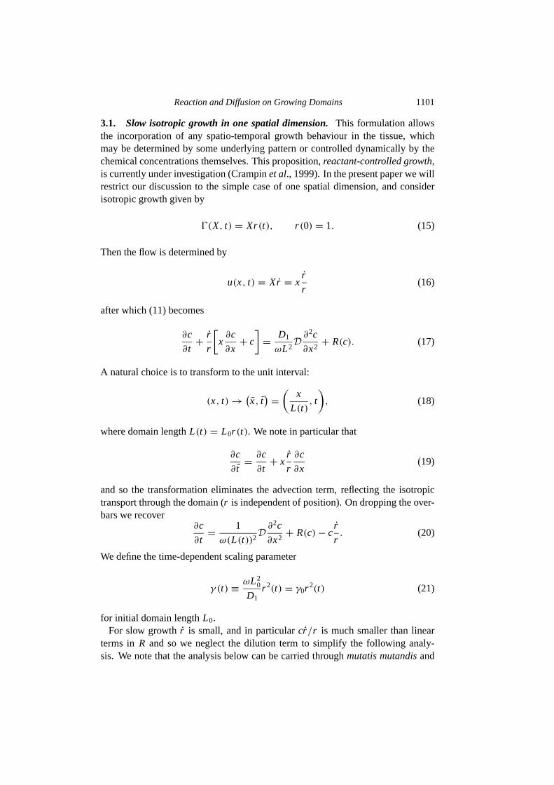
5.2. Role of the kinetic function. The analysis presented above does not de-pend critically on the nonlinear part of the kinetic functionR. Provided that thelinearized kinetics permit diffusion-driven instability and the initial matching ofsolution and construction occurs, then we infer that in general the nonlinearities inthe kinetics do not affect the robustness of the sequence. Simulations of the var-ious kinetic models proposed in the literature have produced frequency-doublingsequences with activator peak splitting or insertion. In Fig.7 we show two suchsequences, with peak splitting in the Schnakenberg scheme (24) and peak insertionfor the model proposed byGierer and Meinhardt (1972)

R=

(ν1c2

2− µ1c1

ν2c22/c1− µ2c2+ δ2

)(34)

where we takeν1 = µ1 = 0.02 andν2 = µ2 = 0.01. In this scheme the kineticspreclude frequency-doubling whenδ2 is identically zero by preventing either formof reorganization of the pattern, also shown in Fig.7. The standard frequency-doubling sequence is recovered for allδ2 6= 0.

It is also possible to generate a sequence in which the pattern undergoes split-ting and insertion of new peaks simultaneously, which will be reported elsewhere.


0 0.5 10

1

2

3

4

5(a)

0 0.5 10

1

2

3

4

5(b)

0 0.5 10

1

2

3

4

5(c)

0 0.5 10

1

2

3

4

5(e)

0 0.5 10

1

2

3

4

5(f)

0 0.5 10

1

2

3

4

5(g)

0 0.5 10

1

2

3

4

5(h)

0 0.5 10

0.5

1

1.5

2(i)

Act

ivat

orA

ctiv

ator

Act

ivat

or

Space0 0.5 1

0

0.5

1

1.5

2(j)

Space0 0.5 1

0

0.5

1

1.5

2(k)

Space0 0.5 1

0

0.5

1

1.5

2(l)

Space

0 0.5 10

1

2

3

4

5(d)

Figure 5. The peak splitting transition between modesm = 2 and4 for equation (22) with Schnakenberg kinetics and exponential growthwith three different values ofρ, the rate-determining parameter, where(a)–(d)ρ = 0.001, (e)–(h)ρ = 0.02 whered = 0.01 and (i)–(l)ρ =0.00001< ρc with d = 0.06 (see text for details). The dotted trace showsthe (symmetrical) tent map acting on the solution atγ /4 [and cannot bedistinguished in (a)–(d)].

This behaviour is generic to purely cubic autocatalysis and is structurally unstableto small quadratic terms, the addition of which recovers the frequency-doublingsequence.

6. OTHER GROWTH FUNCTIONS

Exponential isotropic growth models a population of cells undergoing cell divi-sion at a fixed rate which is independent of spatial or temporal coordinate. Whilethis is a reasonable model of the initial stages of an unconfined growth it is notrealistic for many applications. We can use the same analysis to investigate pat-tern formation under other growth functions. In previous studies various authors


0 1000 2000 3000 4000 5000 6000 7000 8000 9000 10000

0

10

20

(a)

0 100 200 300 400 500 600 700 800 900 1000

0

1

2

φφ

(b)

0 10 20 30 40 50 60 70 80 90 100

0

1

2

Time

φ

(c)

Figure 6. Evolution ofφ(t) for exponential growth with (a)ρ = 0.0005,(b) ρ = 0.005 and (c)ρ = 0.05 showing the departure from two charac-teristic dynamic regimes.

have considered linear growth. Although this may not have a strong biologicalmotivation, studying this growth function gives further insight into the mechanismof pattern sequence formation. We will also consider the biologically plausiblescenario of logistic time dependence, where the final domain size is limited.

6.1. Linear domain growth. For linear growth we haver (t) = 1+ ρt giving

γ (t) = γ0(1+ ρt)2, h(γ ) =dγ

dt= 2ρ√γ0γ . (35)

where for convenience we will takeγ0 = 1. As before we consider the evolutionof a pattern over some interval[γ, 4γ ] such that on eliminatingt the governingequation forc(x,4γ ′; ρ) is

ρ√γ ′∂c

∂γ ′=

1

4γ ′D∂2c

∂x2+ R(c). (36)

Again we consider the frequency-doubled construction, while this time allowingfor a change inρ to find the equivalent equation. Nowq2(x, γ ′; ρ ′) = c(p2(x),


0 0.1 0.2 0.3 0.4 0.5 0.6 0.7 0.8 0.9 10

50100150200

250300350

400450

500

(a)

(b)

(c)

0 0.1 0.2 0.3 0.4 0.5 0.6 0.7 0.8 0.9 1

0024

024

0

5

0.1 0.2 0.3 0.4 0.5

Space

Space

Space

0.6 0.7 0.8 0.9 10

2000

4000

6000

8000 Time

Time

Time

10000

12000

14000

16000

0

2000

4000

6000

8000

10000

12000

14000

16000

Figure 7. Evolution of the activator species for equation (22). Frequency-doubling with (a) activator peak splitting for Schnakenberg kinetics and(b) peak insertion for the Gierer–Meinhardt model withδ2 = 0.001, (c) forwhich δ2 = 0 precludes pattern reorganization.


γ ′; ρ ′) satisfies

2ρ ′√γ ′∂q2

∂γ ′=

1

4γ ′D∂2q2

∂x2+ R(q2) (37)

so thatq2(x, γ ; ρ/2) andc(x,4γ ; ρ) satisfy the same equation.The implication of this result is that prolonged frequency-doubling behaviour is

not a natural consequence of this growth function. However, as before, if thereexists a pointγ = γ ∗ such that

q2(x, γ∗; ρ/2) = c(x,4γ ∗; ρ), (38)

then they coincide for allγ > γ ∗. This implies that if a sequence generated withlinear growth rateρ undergoesM frequency-doubling events before this sequencebreaks up, then a sequence generated at growth rate 2ρ must completeM + 1such events. Numerical evidence confirming this prediction is presented in Fig.8.Although the analysis does not give any information about the sequence after thebreak down of frequency-doubling, numerical solutions suggest that the subsequentbehaviour is not robust, and the sequence may be different for each set of initialconditions.

6.2. Comparisons with exponential domain growth.The quasi-steady regimerequires that the timescale for pattern formation be sufficiently faster than that fordomain growth. We can predict the point of break down of the frequency-doublingsequence under linear growth conditions from knowledge of the lower limit inthe rate-determining parameter,ρc, for the sequence under exponential growth.Comparison of growth rates then suggests that frequency-doubling will occur forlinear growth when

hlin(ρ) ≥ hexp(ρc) (39)

wherehexp = 2ργ andhlin = 2ρ√γ γ0. Then we can derive a condition onγ for

the break down of the sequence, as illustrated in Fig.9, namely

γ ≈ γ0

(ρ

ρc

)2

, (40)

as indicated by the vertical dashed line in the figure.Numerical simulations have confirmed for linear growth that the point of break

down inγ varies approximately with the square ofρ. From equation (40) we seethat higher pattern modes may be admitted prior to the break down of the sequenceonly if ρ is sufficiently larger thanρc. Thus point of break down observed in asequence that initially undergoes frequency-doubling, as given by the intersectionin the figure, corresponds to timet∗ such that

t∗ =1

ρc−

1

ρ≈

1

ρc(41)


00

10

20

30

40

Spac

e

0

10

20

30

40

Spac

e

0

10

20

30

40

Spac

e

50

60

70

80

0

10

20

30

40

Spac

e

50

60

70

80

20.5 1

Time

1.5 0 20.5 1

Time

1.5

0 20.5 1

Time

(a)

1.5 0 20.5 1

Time

(b)

(c) (d)

1.5

Figure 8. Linear domain growth. Space–time evolution of activatorconcentration profilec2(x, t) with Schnakenberg kinetics for (a)ρ =5.0×10−6, (b)ρ = 1.0×10−5, (c)ρ = 2.0×10−5 and (d)ρ = 4.0×10−5

showing 2, 3, 4 and 5 frequency-doubling transitions respectively beforethe sequence breaks down. Transitions appear discontinuous because theyoccur over a time interval much smaller than the total interval shown inthe figures. Other simulations have shown that the remaining pattern se-quence is nonrobust as to which pattern modes it contains and to when thetransitions occur. Time is in units of 106.


0 1 2 3 4 5 6x 105

0

0.2

0.4

0.6

0.8

1

γ

dγ/d

t

Figure 9. Rate of change ofγ for exponential (straight line) and linear(curved line) growth functions. The intersection between the linear growthcurve and the line for exponential growth at the (lower) critical rate param-eterρc is marked with a vertical dashed line. The dotted line representsexponential growth forρ > ρc for which frequency-doubling is observed.

which, forρc ≈ 10−6, is in agreement with the simulations shown in Fig.8. In allcasest∗ falls between the times for the final successful frequency-doubling transi-tion and the subsequent transition which fails to double the spatial frequency.

Analogously to the exponential case, break down of in robustness occurs forρ → 1 through the introduction of an asymmetry during transitions between lowmodes, as the timescales for pattern formation and domain growth coincide.

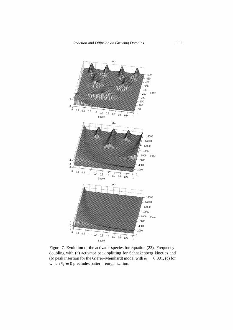
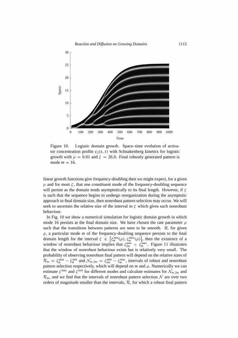
6.3. Logistic domain growth. If the sensitivity of the tissue to the patterningmechanism is confined to a phase of exponential growth, then the previous resultsare sufficient to predict the patterning behaviour. However, if pattern is organizedduring the phase over which the domain growth slows and saturates to achievesome final domain size then we wish to see how this affects pattern formation,and in particular the robustness of the sequence and final pattern that is obtained.Therefore we consider a logistic growth function:

r (t) =exp(ρt)

1+ 1ζ(exp(ρt)− 1)

(42)

such that dr/dt = ρr (1− r/ζ ), whereζ is the ratio of final to initial length.The logistic growth initially looks exponential, but slows to asymptotically ap-

proach the final domain length. If we are in the range for which exponential and


00

5

10

15

Spac

e

20

25

30

100 200 300 400 500

Time

600 700 800 900 1000

Figure 10. Logistic domain growth. Space–time evolution of activa-tor concentration profilec2(x, t) with Schnakenberg kinetics for logisticgrowth withρ = 0.01 andζ = 26.0. Final robustly generated pattern ismodem= 16.

linear growth functions give frequency-doubling then we might expect, for a givenρ and for mostζ , that one constituent mode of the frequency-doubling sequencewill persist as the domain tends asymptotically to its final length. However, ifζ

is such that the sequence begins to undergo reorganization during the asymptoticapproach to final domain size, then nonrobust pattern selection may occur. We willseek to ascertain the relative size of the interval inζ which gives such nonrobustbehaviour.

In Fig. 10 we show a numerical simulation for logistic domain growth in whichmode 16 persists at the final domain size. We have chosen the rate parameterρ

such that the transitions between patterns are seen to be smooth. If, for givenρ, a particular modem of the frequency-doubling sequence persists to the finaldomain length for the intervalζ ∈

[ζmin

m (ρ), ζmaxm (ρ)

], then the existence of a

window of nonrobust behaviour implies thatζmin2m > ζmax

m . Figure11 illustratesthat the window of nonrobust behaviour exists but is relatively very small. Theprobability of observing nonrobust final pattern will depend on the relative sizes ofRm = ζmax

m − ζminm andNm,2m = ζmin

2m − ζmaxm , intervals of robust and nonrobust

pattern selection respectively, which will depend onm andρ. Numerically we canestimateζmax andζmin for different modes and calculate estimates forNm,2m andRm, and we find that the intervals of nonrobust pattern selectionN are over twoorders of magnitude smaller than the intervals,R, for which a robust final pattern


00

1

2

3Spac

e 4

5

6

7

0

1

2

3Spac

e 4

5

6

7

0

1

2

3Spac

e 4

5

6

7

1Time Time Time

2 0 1 2 0 1 2

Figure 11. Logistic domain growth: window of nonrobustness. Space–time evolution of activator concentration profile for Schnakenberg kineticswith logistic growth whereρ = 0.001 andζ = 6.50 ≈ ζmax

4 , ζ = 6.51andζ = 6.52≈ ζmin

8 respectively. Time is in units of 104.

from the frequency-doubling sequence is achieved.

7. DISCUSSION

In this paper we have considered a model of reaction and diffusion on a slowlyand isotropically growing domain which can generate a frequency-doubling se-quence of patterns. This sequence is not sensitive to the conditions specified on theinitial domain and patterns of fast spatial frequency may be reliably generated. Wehave predicted with a self-similarity argument that the sequence arises naturally forexponential growth and we have shown numerically that within a range of the expo-nential growth rate the sequence may continue indefinitely. Under a linear growthfunction the sequence is found to break down after some number of frequency-doubling events, and a relation between the point of break down and the growth rateis established with the self-similarity argument. For logistic growth one element ofthe sequence is selected with high reliability, and will persist as the domain tendsasymptotically to its maximum size. We have neglected a small contribution to thekinetics, which for exponential growth is a time-independent decay term for eachspecies. It is straightforward to show that the self-similarity analysis is unchangedif the term is included, and we have confirmed numerically that the inclusion ofthis term makes only small quantitative changes to the solution behaviour.

In the examples presented in this paper we have taken the initial domain lengthto be below the critical scale for diffusion-driven instability,γ0 < γc. The patternmode observed aftern frequency-doubling events is 2n. However, other sequencesmay be generated for initial domain sizesγ0 > γc such that the first mode to growis m0 > 1, giving rise to the sequencem0 × 2n. If parameters are such that form0

there is no multiplicity of solutions, then a frequency-doubling sequence based onthis mode may also be generated by the mechanism we have described.


We have shown that for the reaction–diffusion model the nonlinearities in the ki-netics determine the mechanism of transformation between modes but the frequen-cy-doubling sequence itself is a generic behaviour. We have found a singular be-haviour in the Gierer–Meinhardt model where, in the absence of a constant acti-vator production term, the pattern reorganization is prevented. We also report thata class of kinetic schemes with purely cubic nonlinearity undergo reorganizationby simultaneous peak splitting and insertion, generating a sequence of frequency-tripling. It is straightforward to show that this behaviour is consistent with the self-similarity analysis we have presented, where now a matching condition is soughtwith the solution under the spatial transformationp3(x) (see Section2.3) and asthe domain triples in length. It is interesting to note that frequency-doubling andtripling have the same dependence on the nonlinear terms as spot and stripe patternformation in two spatial dimensions (Ermentrout, 1991).

The pattern sequences capture a degree of insensitivity to domain length, witheach pattern element in the sequence persisting as the domain doubles in length.This semi-scale invariance is particularly significant in that it allowsregulation, aproperty of many biological systems, whereby a specific number of pattern ele-ments is laid down despite significant variation in the domain size and without theneed to finely tune parameter values. Various authors have considered the problemof scale invariance in reaction–diffusion systems (Othmer and Pate, 1980; Hund-ing and Sørensen, 1988) and have concluded that some form of feedback fromthe domain size into the kinetic parameters is necessary, requiring close parame-ter tolerances. The semi-scale invariance in the present system arises as a naturalconsequence of the sequence formation mechanism.

7.1. Robust pattern generation.In the context of biological pattern formation,and for reliable pattern formation in noisy environments in general, it is essen-tial that the pattern sequence is not be destroyed by external fluctuations. Thefrequency-doubling sequence appears to be insensitive to external spatial perturba-tions imposed as the solution evolves. Simulations in which random perturbationsare superimposed at each time-step produce the same sequence.† The transitionsbetween patterns in a sequence are distinct from the initial bifurcation from the ho-mogeneous steady state and associated pattern selection; they are not noise inducedand the transient (nonquasi-steady) behaviour appears to be determined entirely bythe shape of the evolving solution profile.

We have found that a reaction–diffusion mechanism in one spatial dimensionmay reliably generate an eight-peak pattern (or 16, or 32. . .). This is contrary tothe results ofSaunders and Ho (1995) which are based on the numerical analyses ofa model byArcuri and Murray (1986). In the latter paper the authors do not derive a

†Integration of a fully stochastic equation is required to fully illustrate this point. We predict thatthe frequency-doubling sequence on the exponential domain will be insensitive to noise and that thelinear domain sequence will be insensitive until the sequence breaks down, with subsequent patternmodes being dependent on the noise and initial conditions.


model from first principles but introduce time dependence to the scaling parameterγ , which they also use to rescale the time variable:t = ωτ/γ for dimensionaltime τ . This transformation distorts the relationship between the timescales forpattern growth and domain growth, and consequently their model fails to producethe robust sequences we have found‡. In the present paper we have considered onlypatterning in one spatial dimension, however, the equations derived earlier describereaction and diffusion with arbitrary domain growth and in higher dimensions. Theextension of the current work into two dimensions is in progress. Preliminaryresults are encouraging (Painteret al., 1999), in particular that a rectangular domainwith preferential growth parallel to the longer axis can sustain frequency-doublingof stripes.

7.2. A universal behaviour?. In general, robustness is difficult to obtain for globalpatterning mechanisms which act simultaneously across a fixed domain. Sequen-tial patterning, such as in the mechanism proposed here on the growing domain, ismore reliable. A large family of models of biological pattern formation are basedon lateral inhibition and, as discussed byOster and Murray (1989), have the sameunderlying mathematical explanation for pattern generation. Whether these othermodels exhibit qualitatively similar behaviour in response to growth is the subjectof current investigation.Murray (1993) andGoodwinet al. (1993) have discussedother scenarios in which the pattern selection problem may be overcome. If pat-terning is initiated from one sub-region of a domain, then a global pattern mayform behind a moving front, generally increasing reliability for the selection of thepattern wavelength. Also it has been shown that if several mechanisms are coupledtogether in hierarchical systems such that the steady state solution of one mech-anism becomes the initial condition, or locally determines parameters for anothermechanism, then robustness with respect to initial data may be achieved. Thisscenario is not unlike the mechanism operating for the growing domain.

ACKNOWLEDGEMENTS

EJC acknowledges an earmarked studentship from the BBSRC. EAG is sup-ported by a Wellcome Trust postdoctoral fellowship. Part of this work was sup-ported by the Institute of Mathematics and its Applications (University of Min-nesota) under funds from the National Science Foundation.

‡In fact, exploiting the self-similarity argument one can find a time dependence forγ such that afrequency-doubling sequenceis predicted in Arcuri and Murray’s equations, namelyγ (t) = γ0/(1−ρt). Numerical simulations support this prediction, however, the entire sequence (as far as can beobserved numerically) is confined to the time interval[0, ρ−1).


REFERENCES

Arcuri, P. and J. D. Murray (1986). Pattern sensitivity to boundary and initial conditions inreaction–diffusion models.J. Math. Biol.24, 141–165.

Bard, J. and I. Lauder (1974). How well does Turing’s theory of morphogenesis work?J.Theor. Biol.45, 501–531.

Bentil, D. E. and J. D. Murray (1992). A perturbation analysis of a mechanical modelfor stable spatial patterning in embryology.J. Nonlin. Sci.2, 453–480.

Bunow, B., J.P. Kernevez, G. Joly and D. Thomas (1980). Pattern formation by reaction–diffusion instabilities: applications to morphogenesis inDrosophila. J. Theor. Biol.84,629–649.

Castets, V., E. Dulos, J. Boissonade and P. De Kepper (1990). Experimental evidence of asustained Turing-type nonequilibrium chemical pattern.Phys. Rev. Lett.64, 2953–2956.

Crampin, E. J., E. A. Gaffney, W. W. Hackborn and P. K. Maini. Reaction–diffusionpatterns on growing domains: asymmetric growth. (In preparation.)

De Kepper, P., V. Castets, E. Dulos and J. Boissonade (1991). Turing-type chemical pat-terns in the chlorite-iodide-malonic acid reaction.Physica D49, 161–169.

Dillon, R., P. K. Maini and H. G. Othmer (1994). Pattern formation in generalized Turingsystems I: steady-state patterns in systems with mixed boundary conditions.J. Math.Biol. 32, 345–393.

Ermentrout, B. (1991). Spots or stripes? Nonlinear effects in bifurcation of reaction–diffusion equations on the square.Proc. R. Soc. Lond. A434, 413–417.

Gierer, A. and H. Meinhardt (1972). A theory of biological pattern formation.Kybernetik12, 30–39.

Goodwin, B. C., S. Kauffman and J. D. Murray (1993). Is morphogenesis an intrinsicallyrobust process?J. Theor. Biol.163, 135–144.

Hunding, A. and P. G. Sørensen (1988). Size adaptation in Turing prepatterns.J. Math.Biol. 26, 27–39.

Kondo, S. and R. Asai (1995). A reaction–diffusion wave on the skin of the marine an-gelfishpomacanthus. Nature376, 765–768.

Kulesa, P. M., G. C. Cruywagen, S. R. Lubkin, P. K. Maini, J. Sneyd, M. W. J. Ferguson andJ. D. Murray (1996). On a model mechanism for the spatial pattering of teeth primordiain the alligator.J. Theor. Biol.180, 287–296.

Lacalli, T. C., D. A. Wilkinson and L. G. Harrison (1988). Theoretical aspects of stripeformation in relation toDrosophilasegmentation.Development103, 105–113.

Maini, P. K., K. J. Painter and H. N. P. Chau (1997). Spatial pattern formation in chemicaland biological systems.J. Chem. Soc., Faraday Trans.93, 3601–3610.

Murray, J. D. (1981). A pre-pattern formation mechanism for animal coat markings.J.Theor. Biol.88, 161–199.

Murray, J. D. (1982). Parameter space for Turing instability in reaction diffusion mecha-nisms: a comparison of models.J. Theor. Biol.98, 143–163.

Murray, J. D. (1993).Mathematical Biology, volume 19 ofBiomathematics Texts, 2nd edn,Berlin and London: Springer-Verlag.


Oster, G. F. and J. D. Murray (1989). Pattern formation models and developmental con-straints.J. Exp. Zool.251, 186–202.

Othmer, H. G. and E. Pate (1980). Scale-invariance in reaction–diffusion models of spatialpattern formation.Proc. Natl. Acad. Sci. USA77, 4180–4184.

Painter, K. J., P. K. Maini and H. G. Othmer (1999). Stripe formation in JuvenilePo-macanthusexplained by a generalized Turing mechanism with chemotaxis.PNAS96,5549–5554.

Saunders, P. T. and M. W. Ho (1995). Reliable segmentation by successive bifurcation.Bull. Math. Biol.57, 539–556.

Schnakenberg, J. (1979). Simple chemical reaction systems with limit cycle behaviour.J.Theor. Biol.81, 389–400.

Swindale, N. V. (1980). A model for the formation of ocular dominance stripes.Proc. R.Soc. Lond. B208, 243–264.

Turing, A. M. (1952). The chemical basis of morphogenesis.Phil. Trans. R. Soc. Lond. B237, 37–72.

Varea, C., J. L. Aragon and R. A. Barrio (1997). Confined Turing patterns in growingsystems.Phys. Rev. E56, 1250–1253.

Received 15 February 1999 and accepted 21 June 1999

reaction and diffusion on growing domains: scenarios … publications/109.pdf · reaction and...

Documents