FEDERAL RESERVE BANK OF SAN FRANCISCO

WORKING PAPER SERIES

The views in this paper are solely the responsibility of the authors and should not be interpreted as reflecting the views of the Federal Reserve Bank of San Francisco or the Board of Governors of the Federal Reserve System. This paper was produced under the auspices of the Center for Pacific Basin Studies within the Economic Research Department of the Federal Reserve Bank of San Francisco.

Optimal Reserve Management and Sovereign Debt

Laura Alfaro Harvard Business School

Fabio Kanczuk

Universidade de São Paulo

May 2007

Working Paper 2007-29 http://www.frbsf.org/publications/economics/papers/2007/wp07-29bk.pdf

Optimal Reserve Management and Sovereign Debt*

Laura Alfaro Harvard Business School

Fabio Kanczuk Universidade de São Paulo

May 2007

Abstract

Most models currently used to determine optimal foreign reserve holdings take the level of

international debt as given. However, given the sovereign’s willingness-to-pay incentive problems, reserve

accumulation may reduce sustainable debt levels. In addition, assuming constant debt levels does not allow

addressing one of the puzzles behind using reserves as a means to avoid the negative effects of crisis: why

do not sovereign countries reduce their sovereign debt instead? To study the joint decision of holding

sovereign debt and reserves, we construct a stochastic dynamic equilibrium model calibrated to a sample of

emerging markets. We obtain that the optimal policy is not to hold reserves at all. This finding is robust to

considering interest rate shocks, sudden stops, contingent reserves and reserve dependent output costs.

JEL classification: JEL classification: F32, F33, F34, F4. Key words: foreign reserves, sovereign debt, default, sudden stops. * lalfaro@hbs.edu. Harvard Business School, Boston, MA 02163, Tel: 617-495-7981, Fax: 617-495-5985; kanczuk@usp.br. Department of Economics, Universidade de São Paulo, Brazil. We thank Joshua Aizenman and conversations with Julio Rotemberg for valuable comments and suggestions.

2

1 Introduction

There is a renewed interest in policy and academic circles about the optimal level of foreign

reserves sovereign countries should hold. This recent interest follows the rapid rise in international reserves

held by developing countries. In 2005, for example, reserve accumulation amounted to 20% of GDP in low-

and middle-income countries; whereas this number was close to 5% in high-income countries. This practice

has raised interesting questions in the literature regarding the cost and benefits of reserve accumulation. The

cost of holding reserves has been estimated at close to 1% of GDP for all developing countries (Rodrik

2006).1 Against this cost, an explanation commonly advanced is that countries may have accumulated

reserves as an insurance mechanism against the risk of an external crisis—self protection through increased

liquidity.2

Recently, researchers have undertaken the task of writing analytical models to characterize and

quantify the optimal level of reserves and provide policy advice to countries.3 Most of the formal models

used in the current analysis tend to take the level of international debt as given and solve for the optimal

liquidity-insurance services that reserves can provide. In other words, the literature has set aside the joint

decision of holding sovereign debt and reserves. Although this strategy has allowed for a better

understanding of the interplay between foreign reserves and a sovereign’s access to international markets,

there are several concerns with this approach. First, some of the implications of this assumption may not be

generalized once one considers the joint decision by a sovereign to hold foreign debt and reserves. For

example, in models a la Eaton and Gersovitz (1981), international debt serves an “insurance” role. That is,

the demand for international loans derives from a desire to smooth consumption. Hence, given the

sovereign’s willingness-to-pay incentive problems, additional reserves in this type of models tend to reduce

sustainable debt levels.4 Second, the strategy of assuming constant debt levels does not address one of the

1 Rodrik (2006) estimates the cost of reserves as the spread between the private sector’s cost of short-term borrowing abroad and the yield the Central Bank earns on its liquid foreign assets. 2 For policy advice in this direction, see Feldstein (1999) and Caballero (2003). The “Greensan-Guidotti-IMF” rule proposes full coverage of short-term external liabilities to mitigate the risk of currency crises. 3 See for example Aizenman and Lee (2005), Caballero and Panageas (2004), Jeanne (2007), Jeanne and Ranciere (2006), Lee (2004). 4 In this type of model, the cost to a sovereign of the denial of foreign credit is that the country must resort to other methods for consumption smoothing (such as building stock piles) or it must accept a greater fluctuation in its consumption. This penalty and hence the sustainable levels of foreign debt are higher the greater the cost to the

3

puzzles behind the current accumulation of reserves. Sovereign countries have an alternative way of

reducing the probability and negative effects of external crisis: to reduce the level of sovereign debt. That is,

even in the case where reserve accumulation has positive liquidity benefits in terms of reducing the

probability of suffering financial crises and the output costs associated with it, a similar net asset position

can be obtained by reducing instead the level of foreign debt.5

In this paper, we address these concerns by incorporating debt sustainability issues into the optimal

reserve management analysis. Our main objective is to study the implications of the joint decision of

holding sovereign debt and reserves. We construct a stochastic dynamic equilibrium model of a small open

economy with non contingent debt and reserve assets. Our starting setup is a model a la Eaton-Gersovitz and

similar to Arellano (2006) and Aguiar and Gopinath (2006), but where the sovereign has the choice to hold

reserves. We assess the quantitative implication of the model by calibrating a sample of emerging markets.

A robust result that emerges from our numerical exercises is that the optimal policy is not to accumulate

reserves.

We extend the model in several ways. Most of the recent papers advancing the insurance motive

behind reserve accumulation have been motivated by the sudden loss of access to international capital

markets and the collapse of domestic production which have characterized the emerging markets crises of

the nineties—a phenomenon Calvo (1998) labeled as “sudden stops.”6 In line with the sudden stops

literature, most of the formal analysis studying optimal reserve management model reserve accumulation as

a cushion against external shocks and capital flows reversals while the level of international debt is taken as

given. That is, in these models countries engage in reserve accumulation to seek self-insurance against the

potential tightening of international financial constraints rather than income fluctuation per se as in more

standard debt models. These models have made important progress in providing an integral framework to

analyze quantitatively some of the limitations and risks of the integration of developing countries to

borrower of exclusion. This cost in turn is higher the more limited domestically available options for smoothing consumption are and the lower the cost of smoothing via the international capital markets is (i.e. the lower the world interest rate). See Eaton et al. (1986). 5 Rodrik (2006) mentions that countries could choose instead to reduce short-term debt in order to gain liquidity. More generally, countries can reduce foreign debt. 6 Additional empirical regularities include the sharp contractions in domestic production and consumption and the collapse of the real exchange rate and asset prices. See Arellano and Mendoza (2003) and Edwards (2004) for overviews of the stylized facts and the literature studying the “sudden stops” phenomena.

4

international financial markets.7 But by taking the level of debt as given, they have abstracted from

willingness-to-pay concerns associated with sovereign debt and the sovereign’s choice over the composition

of its assets and liabilities.

In order to analyze the interplay of both effects, we study an economy that is (i) hit by random

shocks in the interest rate (which we take to be “contagion shocks”), and (ii) in addition to the interest rate

shocks, the economy faces additional output costs associated with abrupt current account reversals (which

we take to mean “sudden stops”). However, as mentioned, our model retains willingness-to-pay concerns.

Note that since we focus on debt and reserve management problems, in this paper we do not attempt to

advance the understanding of the contagion or sudden stops phenomena.8 Instead we incorporate them into

the analysis in a highly stylized form. Our approach, nevertheless, reveals interesting results. Once again the

optimal policy does not involve accumulating reserves. Rather, the government reacts by reducing the

amount of outstanding debt. Moreover, these results are robust to the possibility of holding contingent

reserves, which, as suggested by Caballero and Panageas (2005), are a more efficient device to insulate the

country from sudden stops.

We then study the role of output costs. The sovereign debt literature has found output costs to play

an important quantitative role even in models where debt should otherwise be sustainable (see Alfaro and

Kanczuk (2005)). Although these output losses are well documented, their micro-foundation remains to be

understood.9 Nevertheless, some empirical evidence suggests that reserves may reduce the output costs

associated with sudden stops (see Frankel and Cavallo (2004)). In order to incorporate these stylized facts in

our analysis, we consider a case where foreign reserves reduce output costs exogenously. Interestingly, in

this case, if reserves reduce output costs, they reduce sustainability. For this reason, we obtain once again

that it is optimal not to hold reserves.

7 See for example Caballero and Panageas (2004). Estimates by Rodrik (2006) and Jeanne and Ranciere (2006) find reserves holdings to be consistent with a government’s desire to insure against the probability and cost of currency crises. Lee (2004) quantifies the insurance value of reserves. 8 See Mendoza (2004) for important work on this direction. As the author explains, the economics behind sudden stops remains to be understood. The standard real business cycle models do not seem to account for the main stylized facts of these events. Durdu, Mendoza and Terrones (2007) quantitatively analyze the role of foreign reserves in a model of incomplete asset markets in which precautionary saving affects asset holding via business cycle volatility, financial globalization and sovereign risk. 9 See Dooley (2000) and Calvo (2000) for theoretical explanations.

5

The main implication that emerges from our work is that greater attention should be given to the

explicit modeling of additional constraints limiting the sovereign’s ability to reduce debt levels (or more

generally political economy rationales) as they seem necessary towards the understanding of the observed

levels of foreign reserve holdings. To be sure, scholars have considered additional motives for holding

reserves. In an earlier literature, reserve holdings were associated with exchange rate management policies.10

More recently, it has been argued that the rapid rise in reserves has little to do with self insurance, but

instead with the policymaker’s desire to prevent the appreciation of the currency and maintain the

competitiveness of the exporting sector (the mercantilist view by Dooley et al. (2003)).11 Yet, another

strand of the literature has considered political economy issues. Aizenman and Marion (2003), for example,

analyze the role of interest groups, corruption and opportunistic behavior by future policy makers. In their

setup, a policy recommendation to increase international reserve holdings may be welfare reducing as it may

increase the chance of a financial crisis. More generally, our work suggests that policy recommendations

may differ from the consensus once sovereign debt issues are considered. This, is in line with Rogoff`s

(1999) critical remark: “Whereas the debate over why countries repay may seem rather philosophical, it is

quite dangerous to think about grand plans to restructure the world financial system without having a

concrete view on it.”

The rest of the paper is organized as follows. Section 2 presents the benchmark model. Section 3

defines the data and calibration. The results are discussed in section 4, which is complemented by a

comment about the role of reserves as collateral. Section 5 concludes.

2 Model

Our economy is populated by a sovereign country that borrows funds from a continuum of

international risk-neutral investors. The economy faces uncertainty in output. As preferences are concave in

consumption, households prefer a smooth consumption profile. In order to smooth consumption, the

benevolent government may choose optimally to default on its international commitments. As in Arellano 10 See Frenkel and Jovanovic (1981), Edwards (1983) and Aizenman (2005) and Flood and Marion (2002) for recent reviews of the literature. 11 See Aizenman and Lee (2005) for a test of the importance of precautionary and mercantilist motives in accounting for the hoarding of international reserves by developing countries.

6

(2006) and Aguiar and Gopinath (2006), if the government defaults on its debts, it is assumed to be

temporarily excluded from borrowing in the international markets. The novelty of our model is that the

government has available another device to smooth consumption: in addition to issuing debt, the

government can hold international reserves. And even when the government is excluded from borrowing

international funds, a reserve buffer can be used to reduce consumption volatility.

In more precise terms, we assume the sovereign’s preferences are given by

0

( )tt

tU E u c

∞

=

= β∑

with, 1 1( )

(1 )cu c

−σ −=

− σ (1)

where σ > 0 measures the curvature of the utility, β ∈ (0, 1) is the discount factor, and ct denotes household

consumption.

If the government chooses to repay its debt, the country’s budget constraint is given by

1 1exp( ) ( ) ( )B Rt t t t t t t tc z B q B R q R+ += − − + − (2)

where Bt denotes the debt level in period t, Rt denotes the reserve level in period t, and zt is the technology

state in this period, which determines the output level. The debt and reserve price functions, qB(st) and qR(st),

are endogenously determined in the model, and potentially depend on all the states of the economy, st,

which will be described in each of the different scenarios we study. In the benchmark version of the model,

the state of the economy is completely defined by the ordered set st = (Bt, Rt, zt).

We assume the technology state zt can take a finite number of values and evolves over time

according to a Markov transition matrix with elements π (zi , zj ). That is, the probability that zt +1 = zj given

that zt = zi is given by the matrix π element of row i and column j.

When the government chooses to default, the economy’s constraint is

1(1 )exp( ) ( )Rt t t t tc z R q R += − δ + − (3)

where the parameter δ governs the additional loss of output in autarky, a common feature in sovereign debt

models (see Alfaro and Kanczuk (2005a)). After defaulting, the sovereign is temporarily excluded from

7

issuing debt. In particular, we assume that θ is the probability that it regains full access to the international

credit markets.

To grasp some intuition, consider a sovereign’s choice to default, and compare expressions (2) and

(3). On the one hand, defaulting entails an instantaneous reduction in the costs of rolling debt. This means

higher consumption, particularly when the debt service is large. On the other hand, defaulting implies a

lower output, and a reduction in the possibilities of smoothing consumption in future periods. This is

because the sovereign loses access to credit markets. Reserves should have a role in such circumstances,

because they allow for some consumption smoothing even when the sovereign cannot issue debt.

International investors are risk neutral and have an opportunity cost of funds given by ρt, which

denotes the risk-free rate. The investors’ actions are to choose the debt price Btq which depends on the

perceived likelihood of default, and the reserves price Rtq .

For these investors to be indifferent between the riskless asset and lending to a country, it must be

that

(1 )(1 )

B tt

t

q −ψ=

+ ρ (4)

and 1(1 )

Rt

t

q =+ ρ

(5)

where ψt is the probability of default, which is endogenously determined and depends on the sovereign

incentives to repay debt.

The timing of the decisions is as follows. In the beginning of each period, the sovereign starts with

debt level Bt and reserve levels Rt, and receives the endowment exp(zt). She faces the reserve price schedule,

)( tRt sq , and the bond price schedule )( t

Bt sq . Taking these two schedules as given, the sovereign

simultaneously makes three decisions: (i) she chooses the next level of reserves, Rt+1; (ii) she decides

whether to default on her debt or not; and (iii) if she decides not to default, she chooses the next level of

debt, Bt+1.

8

The model described is a stochastic dynamic game. We focus exclusively on the Markov perfect

equilibria. In these equilibria, the sovereign does not have commitment, and players act sequentially and

rationally.

In order to describe the equilibrium, notice first that the international investors are passive, and their

actions can be completely described by equations (4) and (5). In order to write the sovereign problem

recursively, let νG denote the value function of the sovereign if she decides to maintain a good credit history

this period (G stands for bad credit history). Similarly let νB denote the value function of the sovereign once

it defaults (B stands for bad credit history). The value of being in a good credit standing at the start of a

period can then be defined as,

{ , }G Bv Max v v= (6)

This indicates that the sovereign defaults if νG < νB. The value functions νG can be written as,

1( ) { ( ) ( )}Gt t tv s Max u c Ev s += + β (7)

subject to (2), and the value function νB by

1 1( ) { ( ) [ ( ) (1 ) ( )]}B G Bt t t tv s Max u c Ev s Ev s+ += + β θ + − θ (8)

subject to (3).

To compute the equilibrium, it is useful to define a default set as the states of the economy in which

the sovereign chooses to default. The default set in turn determines the prices qB and qR, through expressions

(4) and (5). With these prices at hand, one can solve the sovereign problem (6), (7), and (8). The solution for

(7) determines a default, which can be used in the next iteration.

3 Calibration

We calibrate our model so that each period corresponded to one year. Our list of 28 emerging

economies is composed of those countries classified as such by The Economist.12 We use available data

12 Argentina, Brazil, Chile, China, Colombia, Czech Republic, Egypt, Estonia, Hong Kong, India, Indonesia, Israel, South Korea, Latvia, Lithuania, Malaysia, Mexico, Pakistan, Peru, Philippines, Russia, Saudi Arabia, Singapore, Slovak Republic, Slovenia, South Africa, Turkey, Venezuela.

9

since 1965. To calibrate the technology state z, we estimate an AR(1) process for the (logarithm) of the GDP

for each country i, that is,

, 1 , , 1ln( ) ln( )i t i i t i ty y+ += α + ε , where , (0, )i t iN εε ≈ σ

We obtain that the GDP weighted average (across countries) parameters are α = 0.85 and σε =

0.044, and the dispersion around these values is fairly small. We then assume the technology state can be

discretized into three possible values, zlow, zavg and zhigh. They are spaced so that the extreme values are 2.5

standard deviations away from the mean. We use the Quadrature Method (Tauchen, 1986) to calculate the

transition probabilities. We also discretized the space state of debt and reserves, assuming they could take

values from zero to 60% of GDP. We assumed these grids were large and fine enough not to affect the

decision rules.

We set the probability of redemption θ = 0.5, which implies an average stay in autarky of 2 years, in

line with the estimates by Gelos et al. (2003). In the benchmark case, the output cost is set equal to δ = 10%,

but we experiment with other values as well, δ = 5% and δ = 20% as in Alfaro and Kanczuk (2005a).13

Following the Real Business Cycle literature, we can calibrate the parameter of preference curvature σ = 2

and the risk free rate ρ = 0.04, which corresponds to the U.S. interest rate. As Arellano (2006) and Aguiar

and Gopinath (2006) note, high impatience is necessary for generating reasonable default in equilibrium.

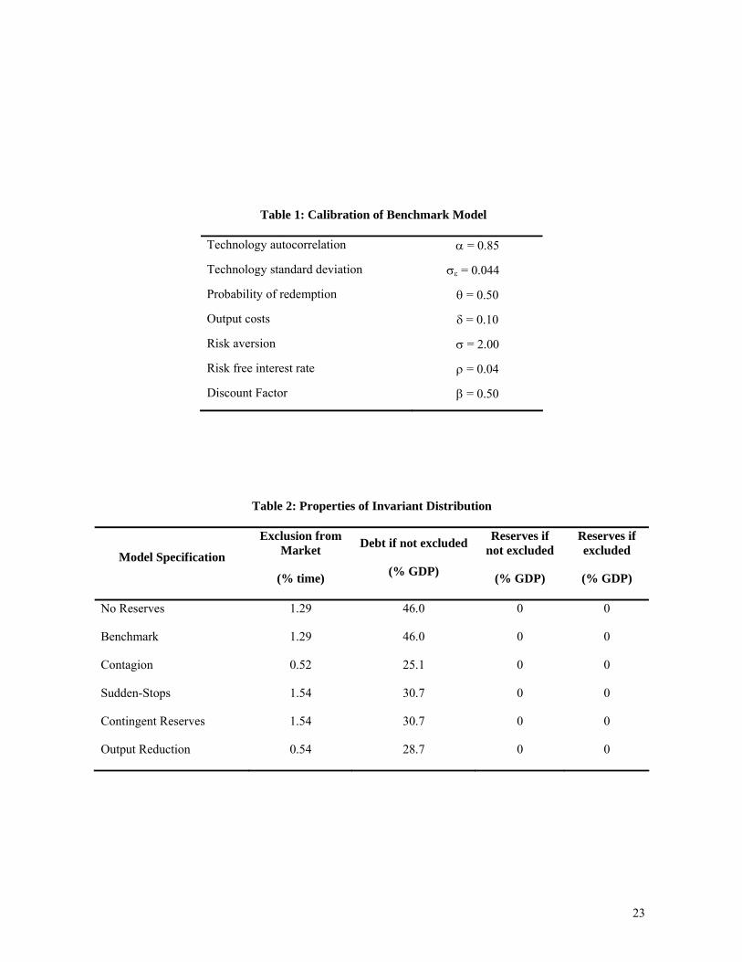
Correspondingly we set the time preference factor equal to β = 0.50. A summary of the calibration

parameters is found in Table 1.

4 Results

4.1 The Model with No Reserves

In order to compare our results with the literature, we first solve for an economy without reserves.

That is, we assume that Rt = 0 for any t, and solve, given the state, for the optimal default choice and for the

optimal level of debt. In this simple case, the state of the economy is completely defined by the asset level

and the technology, st = (Bt, zt).

13 Note that for lower values of δ, the model can sustain very low debt levels relative to the stylized facts.

10

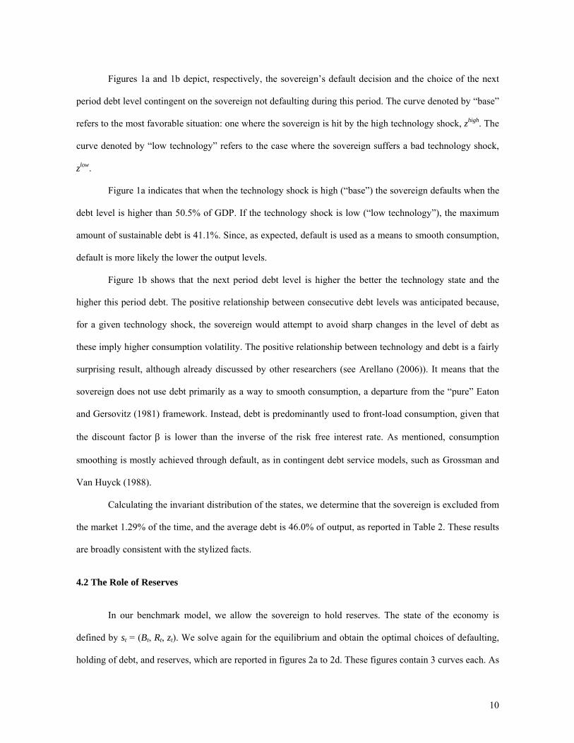
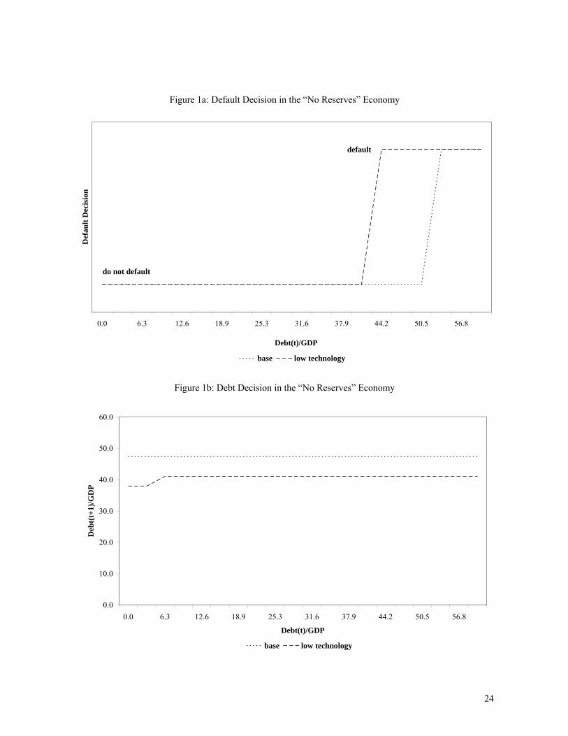
Figures 1a and 1b depict, respectively, the sovereign’s default decision and the choice of the next

period debt level contingent on the sovereign not defaulting during this period. The curve denoted by “base”

refers to the most favorable situation: one where the sovereign is hit by the high technology shock, zhigh. The

curve denoted by “low technology” refers to the case where the sovereign suffers a bad technology shock,

zlow.

Figure 1a indicates that when the technology shock is high (“base”) the sovereign defaults when the

debt level is higher than 50.5% of GDP. If the technology shock is low (“low technology”), the maximum

amount of sustainable debt is 41.1%. Since, as expected, default is used as a means to smooth consumption,

default is more likely the lower the output levels.

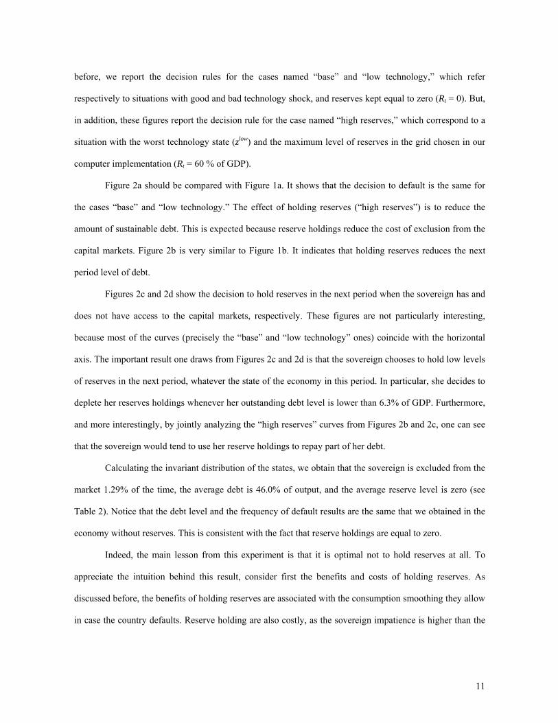
Figure 1b shows that the next period debt level is higher the better the technology state and the

higher this period debt. The positive relationship between consecutive debt levels was anticipated because,

for a given technology shock, the sovereign would attempt to avoid sharp changes in the level of debt as

these imply higher consumption volatility. The positive relationship between technology and debt is a fairly

surprising result, although already discussed by other researchers (see Arellano (2006)). It means that the

sovereign does not use debt primarily as a way to smooth consumption, a departure from the “pure” Eaton

and Gersovitz (1981) framework. Instead, debt is predominantly used to front-load consumption, given that

the discount factor β is lower than the inverse of the risk free interest rate. As mentioned, consumption

smoothing is mostly achieved through default, as in contingent debt service models, such as Grossman and

Van Huyck (1988).

Calculating the invariant distribution of the states, we determine that the sovereign is excluded from

the market 1.29% of the time, and the average debt is 46.0% of output, as reported in Table 2. These results

are broadly consistent with the stylized facts.

4.2 The Role of Reserves

In our benchmark model, we allow the sovereign to hold reserves. The state of the economy is

defined by st = (Bt, Rt, zt). We solve again for the equilibrium and obtain the optimal choices of defaulting,

holding of debt, and reserves, which are reported in figures 2a to 2d. These figures contain 3 curves each. As

11

before, we report the decision rules for the cases named “base” and “low technology,” which refer

respectively to situations with good and bad technology shock, and reserves kept equal to zero (Rt = 0). But,

in addition, these figures report the decision rule for the case named “high reserves,” which correspond to a

situation with the worst technology state (zlow) and the maximum level of reserves in the grid chosen in our

computer implementation (Rt = 60 % of GDP).

Figure 2a should be compared with Figure 1a. It shows that the decision to default is the same for

the cases “base” and “low technology.” The effect of holding reserves (“high reserves”) is to reduce the

amount of sustainable debt. This is expected because reserve holdings reduce the cost of exclusion from the

capital markets. Figure 2b is very similar to Figure 1b. It indicates that holding reserves reduces the next

period level of debt.

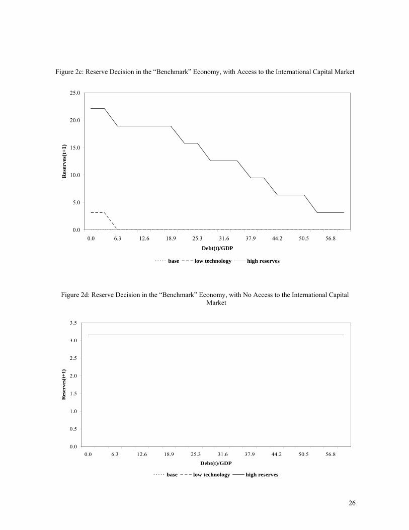
Figures 2c and 2d show the decision to hold reserves in the next period when the sovereign has and

does not have access to the capital markets, respectively. These figures are not particularly interesting,

because most of the curves (precisely the “base” and “low technology” ones) coincide with the horizontal

axis. The important result one draws from Figures 2c and 2d is that the sovereign chooses to hold low levels

of reserves in the next period, whatever the state of the economy in this period. In particular, she decides to

deplete her reserves holdings whenever her outstanding debt level is lower than 6.3% of GDP. Furthermore,

and more interestingly, by jointly analyzing the “high reserves” curves from Figures 2b and 2c, one can see

that the sovereign would tend to use her reserve holdings to repay part of her debt.

Calculating the invariant distribution of the states, we obtain that the sovereign is excluded from the

market 1.29% of the time, the average debt is 46.0% of output, and the average reserve level is zero (see

Table 2). Notice that the debt level and the frequency of default results are the same that we obtained in the

economy without reserves. This is consistent with the fact that reserve holdings are equal to zero.

Indeed, the main lesson from this experiment is that it is optimal not to hold reserves at all. To

appreciate the intuition behind this result, consider first the benefits and costs of holding reserves. As

discussed before, the benefits of holding reserves are associated with the consumption smoothing they allow

in case the country defaults. Reserve holding are also costly, as the sovereign impatience is higher than the

12

reserves remuneration. Or, in other words, in order to build its stock of reserves, an economy has to

consume less.

But, more importantly, reserve holdings endogenously affect the willingness to default of the

sovereign. As a consequence, reserve holdings reduce the amount of “sustainable” debt, or, more precisely,

increases debt services for a given level of debt. Thus, reserve holdings make debt more costly to the

sovereign.

Holding reserves may seem to be suboptimal because the sovereign can, instead, reduce the amount

of outstanding debt. The idea here is that both reserve holdings and less outstanding debt are alternative

ways of achieving consumption smoothing. In bad times, when the economy is hit by a bad output shock, in

order to smooth consumption, the sovereign can increase the amount of debt to its maximum sustainable

level. But in the case when the sovereign has outstanding debt levels lower than the maximum sustainable

level, there is “more room” to borrow before debt becomes unsustainable. (More precisely, since default is

less likely when outstanding debt is smaller, borrowing is relatively cheaper).

However, this logic is too simplistic for many reasons. First, reserves are a device to smooth

consumption even after the country has defaulted, a circumstance in which the country cannot increase debt.

Second, reserves affect the sovereign’s willingness-to-pay in complex ways. And, in particular, there is no

reason for the amount of sustainable debt to vary linearly and uniformly with the amount of reserve

holdings. In other words, there is no guarantee that reducing outstanding debt by, say, X dollars, increases

the ability to smooth the same amount that holding X dollars as reserves does. Third, as Grossman and Han

(1999) show, smoothing consumption through increasing debt is less effective than smoothing consumption

through defaulting. Or, using their typology, “contingent service” generates more consumption smoothing

than “contingent debt.” And since reserves are useful even after defaulting, they can be even more so when

the sovereign opts to pay service contingently.

Taking all these together, one can conclude that there are many reasons why reserves holdings and

less debt outstanding are not perfect substitutes. Consequently, it is not possible to say, a priori, that the

optimal reserve holding is zero. Our result is, therefore, a quantitative one, which depends on the model and

calibration.

13

4.3 Contagion

Is it always optimal to hold no reserves at all? The first robustness for this result we undertake is to

consider the existence of “contagion effects,” or shocks to the international interest rate. The intuition here

is that interest rate shocks may be an additional motivation to default on debt; debt services may become too

costly to the sovereign. And, in as much as defaulting becomes a good alternative, holding reserves becomes

a useful device to smooth consumption in the periods the sovereign is excluded from the international

capital markets.

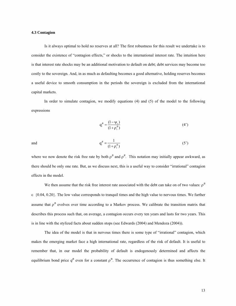
In order to simulate contagion, we modify equations (4) and (5) of the model to the following

expressions

(1 )(1 )

B tt B

t

q −ψ=

+ ρ (4’)

and 1(1 )

Rt R

t

q =+ ρ

(5’)

where we now denote the risk free rate by both ρB and ρR. This notation may initially appear awkward, as

there should be only one rate. But, as we discuss next, this is a useful way to consider “irrational” contagion

effects in the model.

We then assume that the risk free interest rate associated with the debt can take on of two values: ρB

∈ {0.04, 0.20}. The low value corresponds to tranquil times and the high value to nervous times. We further

assume that ρB evolves over time according to a Markov process. We calibrate the transition matrix that

describes this process such that, on average, a contagion occurs every ten years and lasts for two years. This

is in line with the stylized facts about sudden stops (see Edwards (2004) and Mendoza (2004)).

The idea of the model is that in nervous times there is some type of “irrational” contagion, which

makes the emerging market face a high international rate, regardless of the risk of default. It is useful to

remember that, in our model the probability of default is endogenously determined and affects the

equilibrium bond price qB even for a constant ρB. The occurrence of contagion is thus something else. It

14

represents a situation in which the emerging market faces a higher international rate even if it does not

default.

Whereas the risk free rate associated with the debt oscillates, we assume the risk-free rate associated

with reserves is constant and equal to ρR = 0.04. That is, the emerging markets always get the regular (and

thus lower) interest rate remuneration on their reserves, and hence reserve accumulation does not benefit

from the higher interest rates associated with contagion.

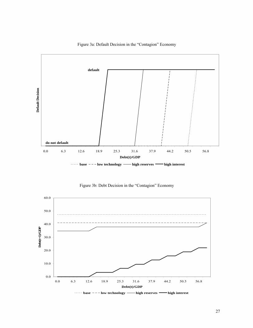
In this specification, the state of the economy is defined by st = (Bt, Rt, zt, ρBt). After solving for the

equilibrium, we can again analyze the policy functions. Figures 3a and 3b depict the default and the next

period of debt choices, and are analogous to Figures 2a and 2b. The curves “base,” “low technology,” and

“high reserves” are defined as before, and refer to the case in which ρB = 0.04, that is, tranquil times. The

additional curve, “high interest,” corresponds to the case with the worst technology shock, with the highest

reserve holdings and with the high international interest rate ρB = 0.20. That is, this curve carries the same

hypotheses of the curve labeled “high reserves” in addition to the interest rate shock or contagion

assumptions.

Notice that the results for the cases “base,” “low technology,” and “high reserves” are the same as

before. The case “high interest” shows that contagion implies that the sovereign opts to default at smaller

debt levels. This could imply more defaults, as one would have expected. However, at the same time,

contagion implies an abrupt reduction in the amount of debt outstanding. Thus, it is not possible, by looking

only at these figures, to know the true impact of contagion on the frequency of defaults.

When we calculate the invariant distribution of the states, we obtain that the sovereign is excluded

from the market only 0.52% of the time, the average debt is 25.1% of output, and the average reserve level

is zero (see Table 2). Thus, contrary to our initial intuition, the sovereign optimally responds to the existence

of contagion by reducing the outstanding debt and defaulting less frequently instead of defaulting more

often. And, as a consequence, reserves again play no role. We chose not to report the decision of reserve

holding (the analogs to curves 2c and 2d) because they do not add additional information. As before, it

suffices to know that the sovereign opts to deplete her reserve holdings for any relevant state of the

economy.

15

4.4 Sudden Stops

A pertinent criticism of our contagion experiment is that it fails to capture some of the most crucial

characteristics of sudden stops. In particular, although we assumed sudden increases in the lending rate, we

have not considered that there might be output costs associated with abrupt reversals in the current account

(or, equivalently, sharp reduction of debt holdings). Maybe because of this, our solution pointed out that the

sovereign would choose to reduce its debt holdings, instead of defaulting.

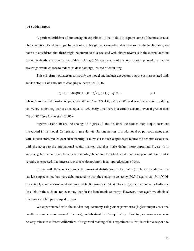
This criticism motivates us to modify the model and include exogenous output costs associated with

sudden stops. This amounts to changing our equation (2) to

1 1(1 )exp( ) ( ) ( )B Rt t t t t t t tc z B q B R q R+ += − Δ − − + − (2’)

where Δ are the sudden-stop output costs. We set Δ = 10% if Bt+1 < Bt - 0.05, and Δ = 0 otherwise. By doing

so, we are calibrating output costs equal to 10% every time there is a current account reversal greater than

5% of GDP (see Calvo et al. (2006)).

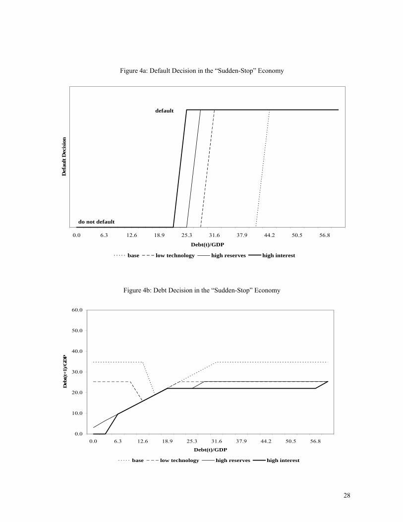
Figures 4a and 4b are the analogs to figures 3a and 3c, once the sudden stop output costs are

introduced in the model. Comparing Figure 4a with 3a, one notices that additional output costs associated

with sudden stops reduce debt sustainability. The reason is such output costs reduce the benefits associated

with the access to the international capital market, and thus make default more appealing. Figure 4b is

surprising for the non-monotonicity of the policy functions, for which we do not have good intuition. But it

reveals, as expected, that interest rate shocks do not imply in abrupt reductions of debt.

In line with these observations, the invariant distribution of the states (Table 2) reveals that the

sudden-stop economy has more debt outstanding than the contagion economy (30.7% against 25.1% of GDP

respectively), and is associated with more default episodes (1.54%). Noticeably, there are more defaults and

less debt in the sudden-stop economy than in the benchmark economy. However, once again we obtained

that reserve holdings are equal to zero.

We experimented with the sudden-stop economy using other parameters (higher output costs and

smaller current account reversal tolerance), and obtained that the optimality of holding no reserves seems to

be very robust to different calibrations. Our general reading of this experiment is that, in order to respond to

16

sudden-stop shocks, the sovereign does not increase the default frequency much but, instead, reduces the

amount of outstanding debt (when compared to the “benchmark” economy outcomes). This, in turn, implies

that sudden-stops are not quantitatively important to rationalize building a reserve buffer.

4.5 Contingent Reserves

In a series of papers, Caballero advocates that emerging markets should hold contingent reserves.14

The intuition is fairly simple. Contingent reserves, which pay higher rates during “sudden stops,” should be

better than non-contingent reserves since they allow for more consumption smoothing. The authors also

describe the conditions for a contingent asset to qualify for this use (it cannot be controlled by the individual

country, and its payoff has to be correlated with the occurrence of sudden stops) and quantify the gains from

its use.15 For the purpose of this paper, the possibility of holding contingent reserves should be seen as an

additional reason to holding a reserve buffer, as it increases its benefits.

In order to simulate the existence of contingent reserves in our economy, we let the price of reserves

take on two values: ρR ∈ {ρLOW, ρHIGH}. We also assume that there is a perfect correlation between ρR and

ρB, that is, ρR = ρLOW when ρB = 0.04, and ρR = ρHIGH when ρB = 0.20. We keep the rest of the model and

calibration identical to the sudden-stop economy.

The fact that international investors are risk neutral implies that there is a restriction on the values of

ρLOW and ρHIGH. Since the expected value of the contingent reserves should be equal to the risk less interest

rate, this pins down ρLOW for a given value of ρHIGH. In order to simulate the economy, we experiment for

different values for ρHIGH. In fact, the choice of ρHIGH corresponds to different leverages, or different blends

of contingent and non-contingent reserves.

However, regardless of the choice of ρHIGH, the result was the same and identical to the case with

non-contingent reserves. That is, the invariant distribution results in the economy with contingent reserves

are equal to those obtained with the sudden-stop economy in the previous subsection. The policy functions

14 See Caballero (2003) and Caballero and Panageas (2004). 15 Caballero and Panageas (2004) have in mind concrete examples of instruments with contingent payoffs. However, more generally one can think that if capital outflows and sudden stops are associated with devaluations, the payoff of reserves (usually denominated in foreign currency) will be negatively correlated with these events.

17

obtained are also identical to those reported in figures 4a and 4b. The contribution of this experiment is that

the benefits from contingent reserves are not quantitatively important enough to reverse to the previous

result. Once again, the optimal reserve holding is zero.

4.6 Output Costs Reduction

Defaulting countries experience output costs beyond the observed reduction in investment and

labor. Alfaro and Kanczuk (2005) find that additional output costs of defaulting are necessary to sustain the

debt levels observed in emerging markets even in a model of contingent services.16 Although these

additional output losses are well documented, their micro-foundation remains to be understood. One

possibility, pointed out by Dooley (2000), is that the loss in output is caused by the inability of debtors and

creditors to quickly renegotiate contracts and the inability to condition the loss of output ex-ante by reasons

of nonpayment. This creates a time interval during which residents of the country in default are unable to

borrow from locals or foreigners, for example, due to the inability of new credits to be credibly senior to

existing credits. If this is factually relevant, then reserves could potentially be used to mitigate the output

costs of default. The empirical evidence provided by Frankel and Cavallo (2004) suggest that reserves may

reduce output costs following a default.17

To investigate the possibility that this could affect our results, we analyze a case where reserves

reduce output costs in an exogenous fashion. To implement this in the model, we change equation (3) to

121

(1 )exp( ) ( )1

Rt t t t t

t

c z R q RR +ω

δ= − + −

+ ω (3’)

Note that the output cost δ was substituted by the expression δ/(1 + ωRtω2

), where ω1 and ω2 are

positive parameters and Rt is the level of reserves (measured in percentage of output). As our benchmark,

we set ω1 = 100 and ω2 = 1, which implies that, when reserves amount to 10% of GDP, the costs from

16 As Grossman and Han (1999) point out, in contingent service models debt is sustainable even if the sovereign can save after defaulting and regardless the existence of additional output costs. 17 Note that although there is a view that foreign reserves might reduce the probability of sudden stops, the overall empirical evidence on this relation is not conclusive (see Calvo et al. (2004), Edwards (2004), Frankel and Cavallo (2004) and Rodrik and Velasco (2000).

18

defaulting halves. We also experimented with ω2 < 1, for which the marginal reduction in the output cost of

the first unit of reserves tends to infinity.18

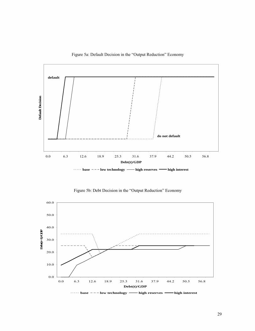
From the solution of the model, we obtain again the policy functions for the default choice and the

next period level of debt, which we depict in Figures 5a and 5b. The most noticeable change is that debt is

now less sustainable than before, as one would expect. The invariant distribution points out to lower debt

levels and fewer defaults (see Table 2). Once again, we obtain that reserve holdings are equal to zero. This

was robust to all values of ω1 and ω2 we tried, including choices such as ω1 = 10000 and ω2 = .5.

Paradoxically, as before, adding a new role for reserves implies in fewer defaults and, thus, no need for

reserves.

4.7 Discussion: Reserves as Collateral

From the point of view of our framework, the main role of reserves is to act as a buffer stock, useful

for consumption smoothing even when the sovereign is excluded from capital markets. As we discussed,

and the quantitative exercises show, according to this view, reserve holdings are consistent with less debt

sustainability. A completely different view, sometimes advanced in the literature, is that reserves can be

used as collateral, thus increasing debt sustainability.

But can reserves really be used as collateral? Our view is that this role, if it exists, is at best very

limited. Reserves are legally protected against attachment by creditors. Under the Foreign Sovereign

Immunities Act of 1976 of the United States and similar laws in other countries, central bank assets,

including international reserves, are usually protected against attachment.19 Hence, reserves work as

collateral only in the case where governments willingly, and more importantly credibly, pledge them as

such.20 Most governments, however, are generally careful to keep their reserve assets untouchable, thus

limiting their role as collateral. As Eaton et al. (1986) note, “if the collateral is retained in the borrowing

18 We thank Joshua Aizenman for this suggestion. 19 This is also the case even when the central bank is the issuer of the debt. The Bank for International Settlements (BIS) in Switzerland is also protected against attachment proceedings; governments and central banks in many cases place assets with the BIS. This, however, is not the case in Germany, where under German law, reserves are open for attachment. See Scott (2005) and Sturzenegger and Zettelmeyer (2006). 20 Reserves, however, can affect the bargaining position of a country in a negotiation. See Detragiache (1996) for a bargaining model that incorporates reserves along these lines.

19

country, there is no mechanism by which the creditor can seize it, and if the collateral is moved outside the

country, where the creditor can seize it, the value of the loan is effectively reduced by the value of the

collateral. A fully and effectively collateralized loan would then be of no value to the borrower.”

5. Conclusions

On the one hand, reserve accumulation is costly because it implies in less current consumption. On

the other hand, holding reserves may be beneficial. Reserves can be used to smooth consumption when a

country (i) is excluded from capital markets after defaulting, (ii) is hit by “irrationally” high interest rates

due to international contagion, or (iii) suffers from a so-called “sudden-stop” phenomenon. In addition,

reserves may be particularly useful (iv) if their payoff is contingent on the state of nature, or (v) if they can

mitigate the output costs associated with a default.

We study the optimal reserve policy in a stochastic dynamic general equilibrium model which is

calibrated to match a typical emerging market economy. The model is general enough to contemplate the

potential benefits of reserves mentioned above and, importantly, endogenously determine the optimal debt

level. We obtain that the optimal policy is not to hold reserves at all.

To obtain our results we resorted to many simplifications. In particular we acknowledge the lack of

micro foundations related to the sudden stop phenomenon. More generally, why countries hold debt remains

to be understood in the literature. We believe that a better understanding of these issues could improve the

analysis, but we do not expect that doing so would change our results qualitatively in terms of the

desirability of reducing the amount of outstanding debt as opposed to increasing reserves.

Overall, our paper contributes to the existing debate by arguing that current reserve holding do not

seem to correspond to the optimal behavior of a sovereign that can both choose the levels of debt and hold

reserves. Some form of transaction costs, which were not considered in our model, could rationalize

countries holding some small amount of reserves, say, to cover for their very short-term debt. But this

cannot account for large reserve stocks. We believe the recent reserve accumulation observed in emerging

markets is better explained by political economy reasons. Exploring these rationales further is an important

topic for future research.

20

6 References

Aguiar, M. and G. Gopinath. 2006. “Defaultable Debt, Interest Rates and the Current Account,” Journal of

International Economics 69, 64-83.

Aizenman, J. 2005. “International Reserves.” In S. N. Durlauf and L. E. Blume, The New Palgrave

Dictionary of Economics, forthcoming.

Aizenman, J. and J. Lee 2005. “International Reserves: Precautionary Versus Mercantilist Views, Theory

and Evidence,” IMF Working Paper 01/198.

Aizenman, J. and N. Marion 2003. “International Reserve Holdings with Sovereign Risk and Costly Tax

Collection,” The Economic Journal 114, 569-591.

Alfaro, L. and F. Kanczuk. 2005. “Sovereign Debt as a Contingent Claim: A Quantitative Approach.”

Journal of International Economics 65, 297-314.

Arellano, C. 2006. “Default Risk and Income Fluctuations in Emerging Markets,” mimeo.

Arellano, C. and E. Mendoza. 2003. “Credit Frictions and ‘Sudden Stops’ in Small Open Economies: an

Equilibrium Business Cycle Framework for emerging Market Crises,” in Dynamic Macroeconomics

Analysis: Theory and Policy in General Equilibrium, Ed. By Altug, Chandha and Nolan, Cambridge

University Press.

Calvo, G. 1998. “Capital Flows and Capital Market Crises: The Simple Economics of Sudden Stops,”

Journal of Applied Economics 1, 35-34.

Calvo, G. 2000. “Balance of Payments Crises in Emerging Markets: Large Capital Inflows and Sovereign

Governments,” in Currency Crises, edited by Paul Krugman. Chicago: The University of Chicago

Press.

Calvo, G., A. Izquierdo and L. Mejia. 2004. “On the Empirics of Sudden Stops: The Relevance of Balance-

Sheet Effects,” NBER Working Paper 10520.

Calvo, G., A. Izquierdo and E. Talvi. 2006. “Phoenix Miracles in Emerging Markets: Recovering without

Credit from Systemic Financial Crises,” NBER Working Paper 12101.

Caballero, R. 2003. “On the International Financial Architecture: Insuring Emerging Markets,” NBER

Working Paper 9570.

21

Caballero, R. and S. Panageas. 2004. “Contingent Reserves Management: An Applied Framework,” mimeo.

Detragiache, E. 1996. “Fiscal Adjustment and Official Reserves in Sovereign Debt Negotiations,”

Economica 63, 81-95.

Dooley, M. 2000. “Can Output Losses Following International Financial Crises be Avoided?” NBER

Working Paper 7531.

Dooley, M., D. Folkerts-Landau and P. Garber. 2003. “An Essay on the Revived Bretton Woods System,”

NBER Working Paper 9971.

Durdu, B., E. Mendoza, and M. Terrones, 2007. “Precautionary Demand for Foreign Assets in Foreign Stop

Economies: An Assessment of the New Mercantilism.” Mimeo.

Eaton, J. and M. Gersovitz. 1981. “Debt with Potential Repudiation: Theoretical and Empirical Analysis,”

The Review of Economic Studies 48, 289-309.

Eaton, J., M. Gersovitz and J. E. Stiglitz. 1986. “The Pure Theory of Country Risk,” European Economic

Review 30, 481-513.

Edwards, S. 1983. “The Demand for International Reserves and Exchange Rate Adjustments: The Case of

LDCs. 1964-1972,” Economica 50, 269-80.

Edwards, S. 2004. “Thirty years of Current Account Imbalances, Current Account Reversals and Sudden

Stops,” IMF Staff Papers 51 (Special Issues), 1-49.

Feldstein, M. 1999. “A Self-Help Guide for Emerging Markets,” Foreign Affairs, March/April 1999.

Flood, R. and P. Marion. 2002. “Holding International Reserves in an Era of High Capital Mobility,” In

Brookings Trade Forum 2001, ed. S. Collins and D. Rodrik. Washington, DC: Brookings Institution

Press.

Frankel, J. and E. A. Cavallo. 2004. “Does Openness to Trade Make Countries More Vulnerable to Sudden

Stops, Or Less? Using Gravity to Establish Causality,” NBER Working Paper 10957.

Frenkel, J. and B. Jovanovic. 1981. “Optimal International Reserves: A Stochastic Framework,” Economic

Journal 91, 507-514.

Gelos, G. R., R. Sahay and G. Sandleris. 2003. “Sovereign Borrowing by Developing Countries. What

Determines Market Access? IMF Working Paper 04/221.

22

Grossman, H. I. and T. Han. 1999. “Sovereign Debt and Consumption Smoothing,” Journal of Monetary

Economics 44, 49-58.

Grossman, H. I. and J. B. Van Huyck. 1988. “Sovereign Debt as a Contingent Claim: Excusable Default,

Repudiation, and Reputation,” American Economic Review 78, 1088-1097.

Jeanne, O. 2007. “International Reserves in Emerging Market Countries: Too Much of a Good Thing.”

Brookings Papers on Economic Activity, forthcoming.

Jeanne, O. and R. Ranciere. 2006. “The Optimal Level of International Reserves for Emerging Market

Economies: Formulas and Applications,” IMF Research Department.

Lee, J. 2004. “Insurance Value of International Reserves: An Option Pricing Approach” IMF Working

Paper 04/175.

Mendoza, E. 2004. “Sudden Stops in a Business Cycle Model with Credit Constraints: A Fisherian

Deflation of Tobin’s Q,” mimeo.

Rodrik, D. 2006. “The Social Cost of Foreign Exchange Reserves,” NBER Working Paper 11952.

Rodrik, D. and A. Velasco. 1999. “Short-Term Capital Flows,” NBER Working Paper 7364.

Rogoff, K. 1999. “Institutions for Reducing Global Financial Instability," Journal of Economic Perspectives

13, 21-42.

Scott, Hal S. 2005. International Finance: Transactions, Policy, and Regulation, 12th Edition. New York:

Foundation Press.

Tauchen, G. 1986. “Finite State Markov-Chain Approximations to Univariate and Vector Autoregressions”

Economics Letters 20, 177-181.

23

Table 1: Calibration of Benchmark Model

Technology autocorrelation α = 0.85

Technology standard deviation σε = 0.044

Probability of redemption θ = 0.50

Output costs δ = 0.10

Risk aversion σ = 2.00

Risk free interest rate ρ = 0.04

Discount Factor β = 0.50

Table 2: Properties of Invariant Distribution

Model Specification

Exclusion from Market

(% time)

Debt if not excluded

(% GDP)

Reserves if not excluded

(% GDP)

Reserves if excluded

(% GDP)

No Reserves 1.29 46.0 0 0

Benchmark 1.29 46.0 0 0

Contagion 0.52 25.1 0 0

Sudden-Stops 1.54 30.7 0 0

Contingent Reserves 1.54 30.7 0 0

Output Reduction 0.54 28.7 0 0

24

Figure 1a: Default Decision in the “No Reserves” Economy

0.0 6.3 12.6 18.9 25.3 31.6 37.9 44.2 50.5 56.8

Debt(t)/GDP

Def

ault

Dec

isio

n

base low technology

default

do not default

Figure 1b: Debt Decision in the “No Reserves” Economy

0.0

10.0

20.0

30.0

40.0

50.0

60.0

0.0 6.3 12.6 18.9 25.3 31.6 37.9 44.2 50.5 56.8

Debt(t)/GDP

Deb

t(t+

1)/G

DP

base low technology

25

Figure 2a: Default Decision in the “Benchmark” Economy

0.0 6.3 12.6 18.9 25.3 31.6 37.9 44.2 50.5 56.8Debt(t)/GDP

Def

ault

Dec

isio

n

base low technology high reserves

default

do not default

Figure 2b: Debt Decision in the “Benchmark” Economy

0.0

10.0

20.0

30.0

40.0

50.0

60.0

0.0 6.3 12.6 18.9 25.3 31.6 37.9 44.2 50.5 56.8

Debt(t)/GDP

Deb

t(t+

1)/G

DP

base low technology high reserves

26

Figure 2c: Reserve Decision in the “Benchmark” Economy, with Access to the International Capital Market

0.0

5.0

10.0

15.0

20.0

25.0

0.0 6.3 12.6 18.9 25.3 31.6 37.9 44.2 50.5 56.8

Debt(t)/GDP

Res

erve

s(t+

1)

base low technology high reserves

Figure 2d: Reserve Decision in the “Benchmark” Economy, with No Access to the International Capital Market

0.0

0.5

1.0

1.5

2.0

2.5

3.0

3.5

0.0 6.3 12.6 18.9 25.3 31.6 37.9 44.2 50.5 56.8

Debt(t)/GDP

Res

erve

s(t+

1)

base low technology high reserves

27

Figure 3a: Default Decision in the “Contagion” Economy

0.0 6.3 12.6 18.9 25.3 31.6 37.9 44.2 50.5 56.8

Debt(t)/GDP

Def

ault

Dec

isio

n

base low technology high reserves high interest

do not default

default

Figure 3b: Debt Decision in the “Contagion” Economy

0.0

10.0

20.0

30.0

40.0

50.0

60.0

0.0 6.3 12.6 18.9 25.3 31.6 37.9 44.2 50.5 56.8

Debt(t)/GDP

Deb

t(t+

1)/G

DP

base low technology high reserves high interest

28

Figure 4a: Default Decision in the “Sudden-Stop” Economy

0.0 6.3 12.6 18.9 25.3 31.6 37.9 44.2 50.5 56.8

Debt(t)/GDP

Def

ault

Dec

isio

n

base low technology high reserves high interest

do not default

default

Figure 4b: Debt Decision in the “Sudden-Stop” Economy

0.0

10.0

20.0

30.0

40.0

50.0

60.0

0.0 6.3 12.6 18.9 25.3 31.6 37.9 44.2 50.5 56.8

Debt(t)/GDP

Deb

t(t+

1)/G

DP

base low technology high reserves high interest

29

Figure 5a: Default Decision in the “Output Reduction” Economy

0.0 6.3 12.6 18.9 25.3 31.6 37.9 44.2 50.5 56.8

Debt(t)/GDP

Def

ault

Dec

isio

n

base low technology high reserves high interest

default

do not default

Figure 5b: Debt Decision in the “Output Reduction” Economy

0.0

10.0

20.0

30.0

40.0

50.0

60.0

0.0 6.3 12.6 18.9 25.3 31.6 37.9 44.2 50.5 56.8

Debt(t)/GDP

Deb

t(t+

1)/G

DP

base low technology high reserves high interest