novel strategies for cleaning-in-place operations · cleaning-in-place (cip) is a widely used...
TRANSCRIPT
General rights Copyright and moral rights for the publications made accessible in the public portal are retained by the authors and/or other copyright owners and it is a condition of accessing publications that users recognise and abide by the legal requirements associated with these rights.
Users may download and print one copy of any publication from the public portal for the purpose of private study or research.
You may not further distribute the material or use it for any profit-making activity or commercial gain
You may freely distribute the URL identifying the publication in the public portal If you believe that this document breaches copyright please contact us providing details, and we will remove access to the work immediately and investigate your claim.
Downloaded from orbit.dtu.dk on: Jun 16, 2020
Novel Strategies for Cleaning-in-Place Operations
Yang, Jifeng
Publication date:2018
Document VersionPublisher's PDF, also known as Version of record
Link back to DTU Orbit
Citation (APA):Yang, J. (2018). Novel Strategies for Cleaning-in-Place Operations. Technical University of Denmark.
DTU Chemical EngineeringDepartment of Chemical and Biochemical Engineering
Novel Strategies for Cleaning-in-Place Operations Jifeng YangPhD thesisNovember 2018
Novel Strategies for Cleaning-in-PlaceOperations
Ph.D. Thesis
Jifeng Yang
Supervisors
Ulrich Krühne (DTU)Krist V. Gernaey (DTU)
Mikkel Nordkvist (Alfa Laval)
Department of Chemical and Biochemical EngineeringTechnical University of Denmark
2800 Kgs. LyngbyDenmark
November, 2018
Copyright©: Søren Heintz
Address:
Phone:
Web:
September 2015
Process and Systems Engineering Center (PROSYS)
Department of Chemical and Biochemical Engineering
Technical University of Denmark
Building 229
Dk-2800 Kgs. Lyngby
Denmark
+45 4525 2800
www.kt.dtu.dk/forskning/prosys
Print: STEP
Jifeng Yang
November 2018
Copyright 2018 Jifeng Yang All rights reserved.
Email: [email protected]
SummaryCleaning-in-place (CIP) is a widely used technique in food and pharmaceutical industries.The execution of CIP is critical for food safety and public health. Since the introductionof CIP, various studies have been performed in order to reduce the cleaning costs withoutcompromising the cleaning quality.
The starting point for this thesis was a mapping study at the world-leading brewery,Carlsberg Danmark A/S (Fredericia), in which the most time- and resource-consumingCIP operations were identified. The suggestions for improving the existing CIP systemsin the brewery are representative for the processes where similar CIP systems are utilizedin other fields. The findings from the mapping study led to the topics explored in thisPh.D study.
The objective of this thesis is to investigate different approaches for reducing the resourceconsumption and cleaning costs during CIP operations. A number of parallel projectswere defined and conducted for this purpose. All of these projects can stand alone whenreading this thesis.
Firstly, a study based on the cleaning of an industrial brewery fermenter demonstrateshow to analyse historical cleaning data to improve cleaning operations in the future. Theproposed analysis approach detects anomalies in a CIP system online and offline. Atrouble-shooting process is advised to guide the operators to diagnose the likely anomalyor fault.
Secondly, Computational Fluid Dynamics (CFD) was used to simulate the displacementof cleaning agent by water during the intermediate and final rinses of pipe systems. Theresults obtained include the identification of dead zones and the calculation of rinsingtime, minimum water consumption, minimum generation of waste water, and pressuredrop, etc. The cross-comparison of different pipe geometries indicates the key factorsthat determine the cleanability of various pipe elements. CFD proves to be an effectivetool for the hygienic design of pipe systems and the optimization of pipe rinsing.
Thirdly, burst cleaning technique to clean the tank surfaces soiled by egg yolk was studied.The experimental observations were compared with the conventional cleaning methodusing continuous flows. Different cleaning parameters were investigated and optimisedfor removing the soil material at the lowest cleaning costs. The primary findings frompilot-scale studies were then examined in scale-up tests.
Fourthly, a three-stage measurement-based partial recovery CIP system was designed.

ii Summary
The purpose of the design was to prolong the lifetime of cleaning liquid by only recyclingthe clear liquid from the CIP outlet. The proposed approach was compared with othercleaning scenarios for economic analysis.
Lastly, the cleaning of toothpaste soil from vessel surfaces by impinging liquid jet andfalling film was studied. The properties of the soil material and the removal force wereinvestigated. The adhesive removal model presented by other researchers was applied todescribe the experimental results. This study is the first work to integrate the effect ofsoil soaking and the cleaning by falling film into the existing model.
Dansk ResumeCleaning-in-place (CIP) er en udbredt teknik inden for fødevare- og farmaceutiske in-dustrier. Gennemførelsen af CIP er meget vigtig for fødevaresikkerhed og folkesundhed.Siden introduktionen af CIP er der blevet foretaget en række undersøgelser for at reducererengøringsomkostningerne uden at gå på kompromis med rengøringskvaliteten.
Udgangspunktet for denne ph.d.-afhandling var en kortlægningsundersøgelse på det ver-densledende bryggeri, Carlsberg Danmark A/S (Fredericia), i hvilket de mest tidskrævendeog ressourcekrævende trin i CIP-operationer blev identificeret. Forslagene til forbedringaf de eksisterende CIP-systemer i bryggeriet kan overføres til processer, hvor lignendeCIP-systemer bruges på andre områder. Resultaterne fra kortlægningsundersøgelsen af-fødte emnerne for dette ph.d.-studie.
Formålet med denne afhandling er at undersøge forskellige metoder til at reducere ressource-forbrug og rengøringsomkostninger under CIP-operationer. En række parallelle projekterblev defineret for at møde dette formål. Alle disse projekter kan stå alene, når man læserdenne afhandling.
Først viser et studie baseret på rengøringen af en industriel bryggerifermenter hvordanman kan analysere historiske rengøringsdata for at forbedre rengøringsprocesserne i fremti-den. Den foreslåede analysemetode gør det muligt at detektere anomalier i et CIP-system,både online og offline. En fejlfindingsproces anbefales for at guide operatørerne til at di-agnosticere sandsynlige anomali eller fejl.
I anden del af afhandlingen bruges Computational Fluid Dynamics (CFD) til at simulerefjernelsen af rengøringsmiddel med vand under mellemliggende og slutskyl af et rørsystem.De opnåede resultater omfatter identifikation af ‘døde’ zoner og beregning af rensningstid,mindste vandforbrug, mindste generening af spildevand og trykfald etc. Sammenligningenaf forskellige rørgeometrier indikerer de nøglefaktorer, der bestemmer rengøringsvenlighe-den af forskellige rørelementer. CFD viser sig at være en effektiv metode til hygiejniskdesign af rørsystemer og optimering af rørrensning.
I tredje del studeres en ‘burst’ rengøringsteknik til rengøring af tankoverflader, der ertilsmudset af æggeblomme. De eksperimentelle resultater sammenlignes med den konven-tionelle rengøringsmetode, hvor der bruges kontinuerligt flow. Forskellige rengøringsparame-tre undersøges og optimeres til fjernelse af smudsmaterialet til de laveste rengøring-somkostninger. De primære resultater fra pilotskalaundersøgelser undersøges herefteri opskaleringstest.
I fjerde del designes et tretrins målebaseret partielt genvinding CIP system. Formålet

iv Dansk Resume
med designet er at forlænge rengøringsvæskens levetid ved kun at genbruge den klarevæske fra CIP udløbsstrøm. Den foreslåede tilgang sammenlignes med andre rengøringscenarier i en økonomisk analyse.
Endelig studeres rensningen af tandpasta fra tankoverflader med jet-væskestråler ogfaldende film. Besmudsningsmaterialets egenskaber og fjernelseskraften undersøges. Denklæbende fjernelses-model fremlagt af andre forskere anvendes til at beskrive de eksperi-mentelle resultater. Denne undersøgelse er det første eksperimentle studie, der integrerereffekten af jordopblødning og rensning med faldende film i den eksisterende model.
PrefaceThis thesis is prepared at the department of Chemical and Biochemical Engineering at theTechnical University of Denmark (DTU) in fulfilment of the requirements for acquiringa Ph.D degree. The project was carried out from December 2015 to November 2018, incooperation with Alfa Laval Copenhagen A/S.
I would like to express my heartfelt gratitude to my academic supervisors Ulrich Krühneand Krist V. Gernaey from DTU, and my industrial supervisor Mikkel Nordkvist fromAlfa Laval. All of them have devoted lots of time and efforts to my work. I keep theiruntiring and sincere teachings in my mind. It has been a great pleasure to work togetherand witness my research progress.
I would also like to thank my industrial collaborators Bo Boye Busk Jensen, Kim Kjell-berg and Jesper Sundwall from Alfa Laval for thoughtful discussions and for helping meto learn advanced technologies. Also, thanks to Peter Rasmussen, Bjarne Pedersen andAnders Kokholm from Carlsberg and Lars Jensen from Ecolab for allowing me to performindustrial on-site studies and sharing their interest and experiences with me. I am alsotruly grateful to Professor Ian Wilson and his Ph.D students Rajesh Bhagat, RubensRosario Fernandes, Melissa Chee, Ru Wang and Harry Ayton at the University of Cam-bridge, who all have made me feel like a part of the team during my research visit in thesummer of 2018.
I have also received help from many other colleagues at the PROSYS Research Group atDTU. I would like to thank everyone who has helped me by answering my questions. Es-pecially, I would like to thank secretary Gitte Læssøe and former secretary Eva Mikkelsenfor helping me with administration stuff, as well as Ph.D students Mengzhe Wu and PauCabañeros López for sharing unforgettable experiences in office 231 in building 227.
This project is part of the INNO+DRIP (Danish partnership for Resource and waterefficient Industrial food Production) project. The fundings from the Innovation FundDenmark (IFD) under Contract 5107-00003B and DTU are acknowledged. The passionateassistance from the partnership manager Hanne Skov Bengaard and the kind discussionswith other collaborators within the partnership are greatly appreciated.
Last but not least, I will never forget the patience and support from my friends and lovingfamily, in particular my wife Wenbo.
Jifeng Yang, November 2018

vi
List of AbbreviationsAFM Atomic Force Microscopy
ANOVA Analysis of Variance
ATP Adenosine TriPhosphate
BLFR Boundary Layer Formation Region
CBR Case Based Reasoning
CFD Computational Fluid Dynamics
CIP Cleaning-In-Place
COD Carbon Oxygen Demand
COP Cleaning-Out-of-Place
CPV Cumulative Percent Variance
CTS Confocal Thickness Sensor
DF Degree of Freedom
DN Nominal Diameter
DoC Degree of Cleaning
DRIP Danish partnership for Resource and water efficient Industrial food Pro-duction project
DTW Dynamic Time Warping
EHEDG European Hygienic Engineering and Design Group
ERT Electrical Resistance Tomography
FDA Functional Data Analysis
FDG Fluid Dynamic Gauge
FN False Negative
FP False Positive
viii List of Abbreviations
FTIR Fourier-Transform Infrared Spectroscopy
GCV Generalized Cross-Validation
MPCA Multiway Principal Component Analysis
NIR Near-InfraRed spectroscopy
NIZO Nederlands Instituut voor ZuivelOnderzoek (Dutch)
PBL Problem-Based Learning
PCA Principal Component Analysis
PENSSE Penalized Sum of Squares
PIV Particle Image Velocimetry
PVC PolyVinyl Chloride
RFZ Radial Flow Zone
RJH Rotary Jet Head
RO Reverse Osmosis
RSH Rotary Spray Head
RSM Response Surface Methodology
RTD Residence Time Distribution
SDBS Sodium Dodecyl Benzene Sulfonate
SEM Scanning Electron Microscope
SRC Stepwise Regression Control
SS Stainless Steel
SSB Static Spray Ball
STD STandard Deviation
TMP Trans-Membrane Pressure
TN True Negative
TOC Total Organic Carbon
TP True Positive
VFD Variable Frequency Drive
WFM Wide-Field fluorescence Microscopy
WSS Wall Shear Stress
ContentsSummary i
Dansk Resume iii
Preface v
List of Abbreviations vii
Contents ix
I Background 1
1 Introduction 31.1 Fouling . . . . . . . . . . . . . . . . . . . . . . . . . . . . . . . . . . . . . 31.2 Cleaning-in-Place . . . . . . . . . . . . . . . . . . . . . . . . . . . . . . . . 41.3 Legislation and Hygienic Design . . . . . . . . . . . . . . . . . . . . . . . . 41.4 CIP System . . . . . . . . . . . . . . . . . . . . . . . . . . . . . . . . . . . 51.5 Assessment of CIP Cleaning Efficiency . . . . . . . . . . . . . . . . . . . . 51.6 Challenges of CIP Optimization . . . . . . . . . . . . . . . . . . . . . . . . 61.7 Thesis Aims and Structure . . . . . . . . . . . . . . . . . . . . . . . . . . 7
2 Literature Review 92.1 Soil Studies . . . . . . . . . . . . . . . . . . . . . . . . . . . . . . . . . . . 9
2.1.1 Soil Types . . . . . . . . . . . . . . . . . . . . . . . . . . . . . . . . 92.1.2 Soil Study Methods . . . . . . . . . . . . . . . . . . . . . . . . . . 102.1.3 Soil Soaking and Swelling . . . . . . . . . . . . . . . . . . . . . . . 12
2.2 Cleaning Mechanisms . . . . . . . . . . . . . . . . . . . . . . . . . . . . . 122.3 The Effects of Cleaning Parameters . . . . . . . . . . . . . . . . . . . . . . 13
2.3.1 Chemistry . . . . . . . . . . . . . . . . . . . . . . . . . . . . . . . . 132.3.2 Temperature . . . . . . . . . . . . . . . . . . . . . . . . . . . . . . 142.3.3 Time . . . . . . . . . . . . . . . . . . . . . . . . . . . . . . . . . . . 152.3.4 Mechanical Force . . . . . . . . . . . . . . . . . . . . . . . . . . . . 152.3.5 Coverage . . . . . . . . . . . . . . . . . . . . . . . . . . . . . . . . 15
2.4 Cleaning Monitoring . . . . . . . . . . . . . . . . . . . . . . . . . . . . . . 162.5 Cleaning Tank Surface and Open Surface . . . . . . . . . . . . . . . . . . 18
2.5.1 Tank Cleaning Devices . . . . . . . . . . . . . . . . . . . . . . . . . 18
x Contents
2.5.2 Cleaning by Impinging Jets . . . . . . . . . . . . . . . . . . . . . . 182.5.3 Cleaning by Falling Films . . . . . . . . . . . . . . . . . . . . . . . 20
2.6 Mathematical Modelling and Data Analysis . . . . . . . . . . . . . . . . . 212.6.1 Predictive Models . . . . . . . . . . . . . . . . . . . . . . . . . . . 22
2.6.1.1 Response Surface Methodology . . . . . . . . . . . . . . . 222.6.1.2 Function Fitting Models . . . . . . . . . . . . . . . . . . . 222.6.1.3 Mechanism-Based Models . . . . . . . . . . . . . . . . . . 242.6.1.4 Kinetics-Based Models . . . . . . . . . . . . . . . . . . . 24
2.6.2 Computational Fluid Dynamics . . . . . . . . . . . . . . . . . . . . 252.6.3 Risk Assessment . . . . . . . . . . . . . . . . . . . . . . . . . . . . 27
2.7 Conclusions . . . . . . . . . . . . . . . . . . . . . . . . . . . . . . . . . . . 28
II Case Studies 31
3 Mapping CIP Systems in a Brewery 333.1 Introduction . . . . . . . . . . . . . . . . . . . . . . . . . . . . . . . . . . . 33
3.1.1 Brewing Process . . . . . . . . . . . . . . . . . . . . . . . . . . . . 333.1.2 Soils in Brewery . . . . . . . . . . . . . . . . . . . . . . . . . . . . 343.1.3 Purpose of Mapping in Carlsberg Danmark A/S . . . . . . . . . . 35
3.2 Methods . . . . . . . . . . . . . . . . . . . . . . . . . . . . . . . . . . . . . 353.3 Mapping Results . . . . . . . . . . . . . . . . . . . . . . . . . . . . . . . . 36
3.3.1 A Cleaning Example . . . . . . . . . . . . . . . . . . . . . . . . . . 363.3.2 Annual Cleaning Costs . . . . . . . . . . . . . . . . . . . . . . . . . 36
3.4 Suggestions for Upgrade . . . . . . . . . . . . . . . . . . . . . . . . . . . . 383.5 Inspirations for This Ph.D Thesis . . . . . . . . . . . . . . . . . . . . . . . 403.6 Conclusions . . . . . . . . . . . . . . . . . . . . . . . . . . . . . . . . . . . 41List of Nomenclature in Chapter 3 . . . . . . . . . . . . . . . . . . . . . . . . . 42
4 Anomaly Analysis in CIP Operations of a Brewery Fermenter 434.1 Introduction . . . . . . . . . . . . . . . . . . . . . . . . . . . . . . . . . . . 434.2 Description of the CIP Practice of a Brewery Fermenter . . . . . . . . . . 444.3 Three-Level Approach for Anomaly Analysis . . . . . . . . . . . . . . . . 454.4 Methods . . . . . . . . . . . . . . . . . . . . . . . . . . . . . . . . . . . . . 46
4.4.1 Feed Pump Analysis . . . . . . . . . . . . . . . . . . . . . . . . . . 464.4.2 Multivariate Monitoring Analysis . . . . . . . . . . . . . . . . . . . 47
4.4.2.1 Functional Data Analysis . . . . . . . . . . . . . . . . . . 474.4.2.2 Alignment of Variable Trajectories . . . . . . . . . . . . . 494.4.2.3 Training and Testing Data Sets . . . . . . . . . . . . . . . 494.4.2.4 Data Unfolding and Normalization . . . . . . . . . . . . . 504.4.2.5 Multivariate Analysis . . . . . . . . . . . . . . . . . . . . 504.4.2.6 Anomaly Detection . . . . . . . . . . . . . . . . . . . . . 514.4.2.7 Anomaly Diagnosis . . . . . . . . . . . . . . . . . . . . . 51
4.4.3 End-of-Batch Performance Evaluation . . . . . . . . . . . . . . . . 524.5 Results and Discussion . . . . . . . . . . . . . . . . . . . . . . . . . . . . . 52
4.5.1 Precleaning: Performance of the Feed Pump . . . . . . . . . . . . . 52
Contents xi
4.5.2 Cleaning or Post Cleaning: Data Pretreatment and MPCA Model 534.5.3 Post Cleaning: End-of-Batch Anomaly Detection and Diagnosis
Based on the Multivariate Analysis . . . . . . . . . . . . . . . . . . 544.5.4 Cleaning: Online Anomaly Detection and Diagnosis Based on the
Multivariate Analysis . . . . . . . . . . . . . . . . . . . . . . . . . 574.5.5 Post Cleaning: Validation of Performance . . . . . . . . . . . . . . 59
4.6 Practical Applications and Future Perspectives . . . . . . . . . . . . . . . 604.7 Conclusions . . . . . . . . . . . . . . . . . . . . . . . . . . . . . . . . . . . 62List of Nomenclature in Chapter 4 . . . . . . . . . . . . . . . . . . . . . . . . . 63
5 Simulations of Blending Phases in Pipe Systems Using CFD 655.1 Introduction . . . . . . . . . . . . . . . . . . . . . . . . . . . . . . . . . . . 65
5.1.1 Blending Phase Problems . . . . . . . . . . . . . . . . . . . . . . . 655.1.2 CFD and Numerical Models . . . . . . . . . . . . . . . . . . . . . . 665.1.3 Objective of This Chapter . . . . . . . . . . . . . . . . . . . . . . . 67
5.2 Methods . . . . . . . . . . . . . . . . . . . . . . . . . . . . . . . . . . . . . 675.2.1 Simulation of Straight Pipes . . . . . . . . . . . . . . . . . . . . . . 67
5.2.1.1 Taylor’s Analytical Model . . . . . . . . . . . . . . . . . . 685.2.1.2 Flow Domain and Mesh . . . . . . . . . . . . . . . . . . . 685.2.1.3 CFD Description . . . . . . . . . . . . . . . . . . . . . . . 695.2.1.4 Mesh Independence Test and Inlet Boundary Conditions 70
5.2.2 Simulation of Complex Geometries . . . . . . . . . . . . . . . . . . 715.2.2.1 Geometries and Model Description . . . . . . . . . . . . . 715.2.2.2 Calculation of Pressure Drop . . . . . . . . . . . . . . . . 71
5.3 Results and Discussion . . . . . . . . . . . . . . . . . . . . . . . . . . . . . 735.3.1 Studies of Straight Pipes . . . . . . . . . . . . . . . . . . . . . . . . 73
5.3.1.1 Studies of Mesh Independence Test and Inlet BoundaryConditions . . . . . . . . . . . . . . . . . . . . . . . . . . 73
5.3.1.2 Comparison of the Taylor Model and CFD Simulations . 745.3.1.3 Displacement Time . . . . . . . . . . . . . . . . . . . . . 755.3.1.4 Minimum Water Consumption for Rinsing . . . . . . . . 785.3.1.5 Minimum Volume of Waste Water . . . . . . . . . . . . . 795.3.1.6 Mixing Zone Length . . . . . . . . . . . . . . . . . . . . . 79
5.3.2 Studies of Complex Geometries . . . . . . . . . . . . . . . . . . . . 825.3.2.1 Dead Zone Identification . . . . . . . . . . . . . . . . . . 825.3.2.2 Pressure Drop . . . . . . . . . . . . . . . . . . . . . . . . 845.3.2.3 Displacement Time . . . . . . . . . . . . . . . . . . . . . 865.3.2.4 Minimum Water Consumption for Rinsing . . . . . . . . 87
5.4 Conclusions . . . . . . . . . . . . . . . . . . . . . . . . . . . . . . . . . . . 88List of Nomenclature in Chapter 5 . . . . . . . . . . . . . . . . . . . . . . . . . 90
6 Cleaning of Egg Yolk Soils from Tank Surfaces Using Burst Flows 936.1 Introduction . . . . . . . . . . . . . . . . . . . . . . . . . . . . . . . . . . . 936.2 Materials and Methods (Pilot-Scale) . . . . . . . . . . . . . . . . . . . . . 94
6.2.1 Experimental Setup . . . . . . . . . . . . . . . . . . . . . . . . . . 946.2.2 Soiling and Cleaning . . . . . . . . . . . . . . . . . . . . . . . . . . 95
xii Contents
6.2.3 Determination of Soiling Areas . . . . . . . . . . . . . . . . . . . . 976.2.4 Factorial Experimental Design . . . . . . . . . . . . . . . . . . . . 976.2.5 Cost Model . . . . . . . . . . . . . . . . . . . . . . . . . . . . . . . 98
6.3 Results and Discussion . . . . . . . . . . . . . . . . . . . . . . . . . . . . . 996.3.1 Cleaning Dynamics . . . . . . . . . . . . . . . . . . . . . . . . . . . 996.3.2 Statistical Comparison of Cleaning by Pulsed Flow or Continuous
Flow . . . . . . . . . . . . . . . . . . . . . . . . . . . . . . . . . . . 1026.3.3 Cleaning of Uncooked Soils with Different Pulsed or Continuous
Approaches . . . . . . . . . . . . . . . . . . . . . . . . . . . . . . . 1066.3.4 Optimization of Cleaning . . . . . . . . . . . . . . . . . . . . . . . 1086.3.5 Cleaning of Cooked Soils with Different Approaches . . . . . . . . 1096.3.6 Cleaning in a Large Scale Tank . . . . . . . . . . . . . . . . . . . . 110
6.4 Conclusions . . . . . . . . . . . . . . . . . . . . . . . . . . . . . . . . . . . 112List of Nomenclature in Chapter 6 . . . . . . . . . . . . . . . . . . . . . . . . . 113
7 A Three-Stage Measurement-Based CIP System for Reducing WaterConsumption 1157.1 Introduction . . . . . . . . . . . . . . . . . . . . . . . . . . . . . . . . . . . 1157.2 Materials and Methods . . . . . . . . . . . . . . . . . . . . . . . . . . . . . 117
7.2.1 Experimental Setup . . . . . . . . . . . . . . . . . . . . . . . . . . 1177.2.2 Soiling . . . . . . . . . . . . . . . . . . . . . . . . . . . . . . . . . . 1187.2.3 Measurements . . . . . . . . . . . . . . . . . . . . . . . . . . . . . 1197.2.4 Cleaning . . . . . . . . . . . . . . . . . . . . . . . . . . . . . . . . . 1197.2.5 Cleaning Costs . . . . . . . . . . . . . . . . . . . . . . . . . . . . . 119
7.3 Results and Discussion . . . . . . . . . . . . . . . . . . . . . . . . . . . . . 1217.3.1 Cleaning Time Against Flow Rate . . . . . . . . . . . . . . . . . . 1217.3.2 Monitoring of Turbidity . . . . . . . . . . . . . . . . . . . . . . . . 1227.3.3 Recovery of Cleaning Water . . . . . . . . . . . . . . . . . . . . . . 1257.3.4 Comparing Cleaning Costs of Different Scenarios . . . . . . . . . . 125
7.4 Conclusions . . . . . . . . . . . . . . . . . . . . . . . . . . . . . . . . . . . 128List of Nomenclature in Chapter 7 . . . . . . . . . . . . . . . . . . . . . . . . . 129
8 Cleaning of Toothpaste from Vessel Surfaces by Impinging Liquid Jetsand Falling Films 1318.1 Introduction . . . . . . . . . . . . . . . . . . . . . . . . . . . . . . . . . . . 1318.2 Model Description . . . . . . . . . . . . . . . . . . . . . . . . . . . . . . . 132
8.2.1 Impinging Jet Introduced Flow Patterns . . . . . . . . . . . . . . . 1328.2.2 Adhesive Removal Model . . . . . . . . . . . . . . . . . . . . . . . 1338.2.3 Cleaning Model of Static Jet . . . . . . . . . . . . . . . . . . . . . 1348.2.4 Cleaning Model of Moving Jet . . . . . . . . . . . . . . . . . . . . 1348.2.5 Cleaning Model of Falling Film . . . . . . . . . . . . . . . . . . . . 137
8.3 Materials and Methods . . . . . . . . . . . . . . . . . . . . . . . . . . . . . 1388.3.1 Rheology . . . . . . . . . . . . . . . . . . . . . . . . . . . . . . . . 1388.3.2 Millimanipulation . . . . . . . . . . . . . . . . . . . . . . . . . . . 1388.3.3 Impinging Jet Apparatus and Experimental Design . . . . . . . . . 1398.3.4 Film Thickness . . . . . . . . . . . . . . . . . . . . . . . . . . . . . 140
Contents xiii
8.3.5 Cleaning by Static Jets . . . . . . . . . . . . . . . . . . . . . . . . 1418.3.6 Cleaning by Moving Jets . . . . . . . . . . . . . . . . . . . . . . . . 1418.3.7 Cleaning by Falling Films . . . . . . . . . . . . . . . . . . . . . . . 141
8.4 Results and Discussion . . . . . . . . . . . . . . . . . . . . . . . . . . . . . 1438.4.1 Rheology Measurement . . . . . . . . . . . . . . . . . . . . . . . . 1438.4.2 Millimanipulation Measurement . . . . . . . . . . . . . . . . . . . . 1448.4.3 Cleaning Behaviour - Static Jet . . . . . . . . . . . . . . . . . . . . 1458.4.4 Cleaning Behaviour - Moving Jet . . . . . . . . . . . . . . . . . . . 1478.4.5 Measurement of Film Thickness . . . . . . . . . . . . . . . . . . . . 1498.4.6 Cleaning Behaviour - Falling Film . . . . . . . . . . . . . . . . . . 150
8.5 Conclusions . . . . . . . . . . . . . . . . . . . . . . . . . . . . . . . . . . . 154List of Nomenclature in Chapter 8 . . . . . . . . . . . . . . . . . . . . . . . . . 155
III Conclusions and Perspectives 159
9 Overall Conclusions 161
10 Perspectives 16310.1 Suggestions for Future Work . . . . . . . . . . . . . . . . . . . . . . . . . . 16310.2 Other Opportunities for Improving Industrial CIP Operations . . . . . . . 164
10.2.1 Smart Scheduling of Production and Cleaning . . . . . . . . . . . . 16410.2.2 Membrane Technology . . . . . . . . . . . . . . . . . . . . . . . . . 16510.2.3 Novel Cleaning Agents . . . . . . . . . . . . . . . . . . . . . . . . . 165
10.2.3.1 Enzyme-Based Cleaner . . . . . . . . . . . . . . . . . . . 16510.2.3.2 Electrolysed Water . . . . . . . . . . . . . . . . . . . . . . 166
10.2.4 Pigging Technology . . . . . . . . . . . . . . . . . . . . . . . . . . . 166
IVAppendices 167
A Dead Zone Identifications of Various Pipe Elements by CFD 169
B Cleaning Dynamics of Egg Yolk Soils from Tank Surfaces (All Data) 173
C The Development of Flow Channels During the Cleaning of Tooth-paste by Falling Films 175
List of Publications 177
Bibliography 179

xiv

Part I
Background

CHAPTER1Introduction
Fouling is a critical problem in food and pharmaceutical industries. Cleaning aims toremove the product residuals and fouling materials that remain in the process line afterproduction. The act of cleaning is crucial to ensure product quality and productionsafety. Industrial users often expect to minimize the cleaning costs without compromisingcleaning quality. The purpose of this chapter is to present:
1. Fouling problems in industries;
2. The definition and implementation of cleaning-in-place;
3. Legislative guidelines of cleaning and hygienic design;
4. Typical cleaning-in-place systems;
5. The definition of cleaning assessment methods;
6. Typical challenges in the studies of cleaning;
7. The aim and structure of this thesis.
1.1 FoulingDuring the production and transfer of food and pharmaceuticals, materials stick to thesurfaces of the equipment and pipes. This build-up process is known as fouling. Theseunwanted material depositions, called soils, need to be removed before the next productioncan take place. Fouling is formed due to the adhesion of materials to the surfaces aswell as the cohesion between elements of the materials being processed [1]. Fouling canbe classified according to the means of formation, such as crystallization, particulatedeposition, biological growth, chemical reaction, corrosion and freezing or solidification[2, 3].
Fouling results in increased operating costs of equipment. Moreover, a potential cross-contamination can threaten the product quality, which can be catastrophic to publichealth and operational safety. Therefore, cleaning is of great significance to the food andpharmaceutical industries. It is estimated that, for a food and beverage plant, nearly20% of each work day is spent on cleaning [4].
4 1 Introduction
1.2 Cleaning-in-PlaceCleaning-in-Place (CIP) is now a common cleaning practice for pipe systems, vessels,filters, process and associated equipment. It originated in the 1950s on dairy farms andwas adopted by the brewing, dairy, beverage, pharmaceutical and food industries duringthe subsequent 15 years [5]. The concept of CIP is to clean the components of a plantwithout dismantling or opening the equipment, and with little or no manual involvementof operators.
Typical CIP systems utilize vessels for the storage and recovery of cleaning solutions. Aseries of pipelines, pumps, along with valves and field instruments are used to transferand control the flows of liquids. The cleaning efficiency and cost effectiveness dependon the complexity and degree of automation of the cleaning system. Cleaning processes,either manual or automated and in all industries, tend to consist of a series of similarsteps, including [6]:
1. Product recovery to drain product from the system;
2. Pre-rinse to remove excessive soils by using water;
3. First detergent circulation to loosen soils from surfaces and dissolve or suspend thesoils in the alkaline detergent solution;
4. First intermediate rinse to remove the first detergent and entrained soils by meansof water;
5. Second detergent circulation to remove harsher soils or mineral scales by acid;
6. Second intermediate rinse to remove the second detergent and soils by means ofwater;
7. Disinfection (optional) to kill microorganisms if sterile or aseptic environment isrequired for subsequent processes;
8. Final rinse to remove residual cleaning and/or disinfection agents.
CIP is more suitable than conventional manual cleaning methods for large scale opera-tions, where complex plant and equipment are involved. CIP allows for high temperature,high chemical concentration and harsh chemicals, which are difficult to apply in manualcleaning operations.
1.3 Legislation and Hygienic DesignThe design of food processing equipment requires the equal consideration of productionpurpose and cleaning possibility. The criteria for the hygienic design of food processingequipment have been described by the Machinery Directive 2006/42/EC and the amend-ing Directive 2009/127/EC, part of which has been incorporated in the standards EN1672-2:2005+A1:2009 and EN ISO 14159:2008 [7]. The European Hygienic Engineering
1.4 CIP System 5
and Design Group (EHEDG) provides guidelines as authority on hygienic engineeringand design. It is created by an international expert panel with diverse representativesof equipment manufacturers, food industries, research institutes and public health au-thorities. The EHEDG offers standardized tests for the cleanability of components. Inthe USA, prescriptive standards for dairy production have been amended for equipmentdesign and sanitation, called 3-A standards. These standards are also adopted in otherbranches in the food industries in the USA. The ASME BPE standard used for Biopro-cessing Equipment provides guidelines applicable to the specific parts with relatively highlevels of hygienic requirements.
Stainless steel is the most frequently used material for processing equipment. In the hy-gienic industries, the selected stainless steel should meet the requirement: carbon content(C) ≤ 0.05%, molybdenum content (Mo) ≥ 2.0%. The inside surface roughness should bewith the acceptance criterion of Ra ≤ 0.8 µm [8]. The tanks, pipes, internal angles andcorners need to be mounted to be fully drainable, or with drain valves installed as low aspossible. Dead spaces shall be avoided, or at least should be capable of performing propercleaning and disinfection. However, in reality, some production plants are not completelyhygienically designed, especially when a new system is built by adding onto an existinglayout. Therefore, the inspection of pipes and equipment is suggested periodically fordetecting the potential defects or weaknesses.
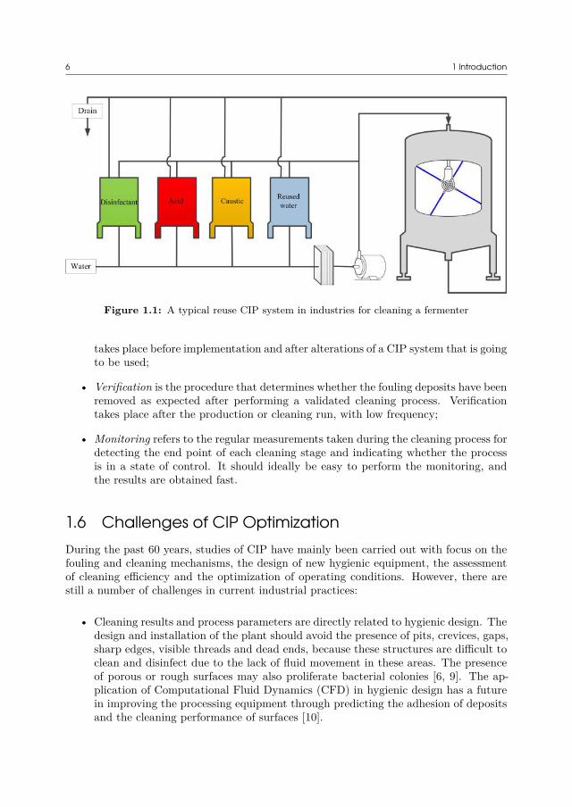
1.4 CIP SystemIn all hygienic industries (e.g., food, beverage, pharmaceutical), similar CIP systemsand equipment are used in CIP practices. Typical CIP systems can be divided intosingle-use and reuse [6]. For a single-use CIP system, the cleaning medium needs tobe prepared freshly, and drained after finishing cleaning. The single-use CIP systemshould be installed as close as possible to the facilities that need to be cleaned. Itreduces the possibility of cross-contamination and potential spore formation, which ismore hygienic and flexible than the reuse CIP system. But single-use systems tend tobe very expensive to operate. For a reuse CIP system, the cleaning medium is recoveredpartially or completely, depending on whether an intermediate storage is used or not. Thistype of system usually comprises large storage tanks and one or more recovery loops, asshown in Figure 1.1. The tanks and associated pipes and instruments to be cleaned canbe cleaned simultaneously without delay.
1.5 Assessment of CIP Cleaning EfficiencyThe assessment of cleaning efficiency can be divided into validation, verification andmonitoring [6].
• Validation ensures that the information supporting the cleaning process is correct.It is the method that determines whether the cleaning process is correct. Validation
6 1 Introduction
Figure 1.1: A typical reuse CIP system in industries for cleaning a fermenter
takes place before implementation and after alterations of a CIP system that is goingto be used;
• Verification is the procedure that determines whether the fouling deposits have beenremoved as expected after performing a validated cleaning process. Verificationtakes place after the production or cleaning run, with low frequency;
• Monitoring refers to the regular measurements taken during the cleaning process fordetecting the end point of each cleaning stage and indicating whether the processis in a state of control. It should ideally be easy to perform the monitoring, andthe results are obtained fast.
1.6 Challenges of CIP OptimizationDuring the past 60 years, studies of CIP have mainly been carried out with focus on thefouling and cleaning mechanisms, the design of new hygienic equipment, the assessmentof cleaning efficiency and the optimization of operating conditions. However, there arestill a number of challenges in current industrial practices:
• Cleaning results and process parameters are directly related to hygienic design. Thedesign and installation of the plant should avoid the presence of pits, crevices, gaps,sharp edges, visible threads and dead ends, because these structures are difficult toclean and disinfect due to the lack of fluid movement in these areas. The presenceof porous or rough surfaces may also proliferate bacterial colonies [6, 9]. The ap-plication of Computational Fluid Dynamics (CFD) in hygienic design has a futurein improving the processing equipment through predicting the adhesion of depositsand the cleaning performance of surfaces [10].
1.7 Thesis Aims and Structure 7
• Despite the high automation of current CIP systems, most cleaning operations pro-ceed semi-empirically and far from optimal. This is because (1) the confirmationof cleanliness is mostly achieved by offline measurement in an open-loop control,and (2) there is no effective measurement method to exactly detect the end pointof cleaning [11]. Therefore, current CIP systems are normally controlled with fixedcleaning times and/or fixed volumes of cleaning agents [12]. The cleaning timeis merely predictable using a series of adjustable variables [5], and usually deter-mined from experience. Thus, excessive amounts of water and chemicals are usedin order to ensure complete cleanliness, which causes large operating costs and highenvironmental impact.
• Cleaning operations generate large amounts of waste water containing corrosivepollutants, nutrients, organic loadings, biochemical oxygen components and heat.Minimizing the environmental impact of cleaning has become of great importancedue to the legislative pressure towards the establishment of zero emission processes[13]. In addition to waste water treatment, another possibility is to take into accountthe mass balance and energy balance in the whole system. This can be realizedthrough three steps: (1) investigating the current water balance; (2) optimizingthe water consuming processes; and (3) optimizing the overall process with zerodischarge of water and the minimal consumption of energy [14].
• It is problematic to compare and transfer results from lab scale experiments toindustrial scale equipment. The deposits observed in experiments are often notrepresentative of real soils. The relationship between the cleaning rate and theeffectiveness of cleaning at different scales is still unclear [15].
• In some industries, the CIP systems have been employed for many years and arerelying on outdated methods. Early CIP systems typically had a one-size-fits-allcleaning cycles. But the different sets of processing equipment need individual CIPrecipes and cleaning requirements. In addition, the age of pipelines and the rear-rangement of process equipment have often reduced the efficiency of the originallydesigned CIP capacity, which requires the renovation of the pipes. Meanwhile, aCIP process should be considered together with the production process in order toachieve the final goal of an efficient, robust, and validated CIP operation, namedintegrated CIP design.
1.7 Thesis Aims and StructureThis Ph.D project is a part of the INNO+DRIP (Danish partnership for Resource and wa-ter efficient Industrial food Production, http://drippartnership.com/) project. Thepartnership involves a number of food companies and technology providers, three univer-sities and two GTS institutes (research and technology organizations). The ambition ofINNO+DRIP project is to produce more with less water at leading Danish food producers.The goal is a reduction in water consumption of 15 – 30%.
The objective of this Ph.D thesis is to shed light on the opportunities for reducing waterusage during CIP. This Ph.D work was performed in close collaboration with the partners
8 1 Introduction
including a technology provider, a food end-user, a chemical supplier and an academicpartner. The primary intention of the project is to provide practical solutions for savingcleaning costs in industrial CIP applications.
This thesis is divided into three parts. Part I (Chapters 1 and 2) focuses on the back-ground including the basic knowledge of CIP and the present status of the researchactivities about CIP. Part II (Chapters 4 to 8) describes the research conducted in thisPh.D work. Each chapter can be read separately and some are written as scientific articleswith additional information added in the thesis. Chapter 3 describes a mapping studyof the CIP systems in a brewery and serves as an introduction to the following investiga-tions. Chapters 4 and 5 aim to optimize existing CIP operations by analysing industrialmonitoring data and simulating the displacement process in pipe systems. Chapters 6to 8 are focused on designing new CIP systems. The conclusions and perspectives of thiswork are presented in Part III (Chapters 9 and 10).
In this thesis, a “List of Abbreviations” (pages vii - viii) summarizes all abbreviationsappearing in the whole thesis. Each chapter contains its own nomenclature, where some-times the same letters are used in different chapters but have different meanings.

CHAPTER2Literature Review
Chapter 1 has highlighted the challenges encountered during the industrial implementa-tion of CIP. This thesis aims to investigate different approaches for reducing resourceconsumption and cleaning costs during CIP operations. To achieve this, a literaturereview in this chapter is conducted, including:
1. The understanding of soil materials and study methods;
2. The cleaning mechanisms for typical soil types;
3. The effects of different cleaning parameters on the cleaning performance;
4. The monitoring techniques for measuring a cleaning process online or offline;
5. The studies and techniques about tank cleaning and open surface cleaning;
6. The application of mathematical modelling and data analysis tools in cleaning stud-ies;
2.1 Soil Studies
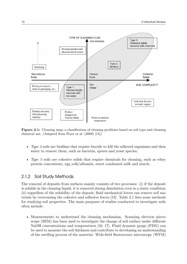
2.1.1 Soil TypesFouling is a result of the adhesion of species to a surface and the cohesion between theelements contained in the deposits [1]. According to the complexity of the physiochemicalproperties of the soils and the types of cleaning fluid, cleaning problems can be classifiedthrough a diagram representation (Figure 2.1) [15].
The horizontal axis in Figure 2.1 indicates the soil complexity ranging from non- orlow-viscosity fluids to high viscous fluids and even cohesive solids. The vertical axisdetermines which fluid should be used for cleaning, including cold water, hot water andhot chemical solutions. Figure 2.1 demonstrates that clusters of similar problems arefound with respect to cleaning issues from the food and personal care product industries.According to Fryer et al. (2009), the shaded area shows three types of soils that are mostdifficult to clean [15]):
• Type 1 soils refer to viscous or viscoelastic or viscoplastic fluids that can be removedby water, such as toothpaste, shampoo, cream and mustard;
10 2 Literature Review
Figure 2.1: Cleaning map; a classification of cleaning problems based on soil type and cleaningchemical use. (Adapted from Fryer et al. (2009) [15])
• Type 2 soils are biofilms that require biocide to kill the adhered organisms and thenwater to remove them, such as bacteria, spores and yeast species;
• Type 3 soils are cohesive solids that require chemicals for cleaning, such as wheyprotein concentrate, egg yolk/albumin, sweet condensed milk and starch.
2.1.2 Soil Study MethodsThe removal of deposits from surfaces mainly consists of two processes: (i) if the depositis soluble in the cleaning liquid, it is removed during dissolution even in a static condition;(ii) regardless of the solubility of the deposit, fluid mechanical forces can remove soil ma-terials by overcoming the cohesive and adhesive forces [13]. Table 2.1 lists some methodsfor studying soil properties. The main purposes of studies conducted to investigate soilsoften include:
• Measurements to understand the cleaning mechanism. Scanning electron micro-scope (SEM) has been used to investigate the change of soil surface under differentNaOH concentrations and temperatures [16, 17]. Fluid dynamic gauge (FDG) canbe used to measure the soil thickness and contribute to developing an understandingof the swelling process of the material. Wide-field fluorescence microscopy (WFM)

2.1 Soil Studies 11
Table 2.1: Summery of soil study methods
Techniques Characteristics Soil types and references
SEM Surface topography Whey and whole milk protein[16, 17]; Bacillus spores [19]
FDG Soil thickness
Egg yolk [20]; Gelatine and eggyolk [21]; β-lactoglobulin geland whey protein [22]; Whey
protein [23]; Bacillus spores [19]
WFM Fluorescence of proteins Whey protein hydrogels labelledwith fluorescent tracer [24]
Micromanipulation Cohesive force andadhesive force Egg albumin [25]
Millimanipulation Cohesive force andadhesive force Carbohydrate-fat food soil [26]
AFM Adhesive force
Whey protein concentrate [27];Toothpaste, sweetened
condensed milk, Turkish delightand caramel [18]
Rheology Viscosity; Yield stress;Microstructure property
Toothpaste [28]; Food product(i.e., dairy, emulsion gels) [29]
Microindenter Shear modulus Whey protein hydrogels [30]
can also provide swelling and dissolution information by detecting the protein con-centration in the liquid phase.
• Measuring the required force to remove deposits from surfaces. Both micromanipu-lation and millimanipulation techniques have been developed to study the adhesiveand cohesive forces required to deform and displace soil layers. The latter canmeasure larger forces and deeper layers than the former. Atomic force microscopy(AFM) is more sensitive to determine adhesive forces and can work in nano-scale,which can help the studies of anti-fouling surfaces [18].
• Measuring the internal properties of deposits. The application of rheology mea-surement and microindenter provides information about the structural change ofsoils for example by soaking. The understanding of the internal resistance of soil isvaluable to select an optimal cleaning method.
There are also spectroscopic techniques available to investigate biofilms, such as confocalmicroscopy, reflective Fourier-transform infrared spectroscopy (FTIR) and near-infraredspectroscopy (NIR). However, the application of these methods has yet to be reportedbecause of the challenges of speed, resolution, and cost [31].
12 2 Literature Review
2.1.3 Soil Soaking and SwellingFundamentally, the cleaning process of protein or starch deposits consists of three phases[23, 32]. First, the initially dry soil contacts with the cleaning liquid and swells to bea weakened and mobilised soil layer. The removal rate in this phase is insignificant.Second, the weakened layer is exposed to mechanical stress and chunks of deposits areremoved at a high rate. The main mechanism in this phase could be viscous shifting orcohesive separation. Third, the cleaning mechanism switches to the decay phase, wherethe removal of small soil particles is limited by the continuous diffusive swelling process.This induces a substantial increase in the time scale.
Swelling comes together with soaking, which is a combined result of chemistry, tempera-ture and time. As a consequence, the force required for cleaning can be reduced greatly.For example, the force to detach carbohydrate-fat based soil is reduced by 95% aftersubmerging the dry material into sodium dodecyl benzene sulfonate (SDBS) solutions.The understanding of soaking and swelling helps to implement burst technology in tankcleaning and to design new tank cleaning devices for example by combining the advan-tages of liquid fans to wet the soil and nozzles to mechanically detach the soil in onerotary jet head [33]. The concept of burst cleaning is to perform cleaning operations byinterrupting a continuous flow with several breaks between shots of fluid, with the goalto reduce cleaning cost by using less chemicals to achieve a certain level of cleanliness.
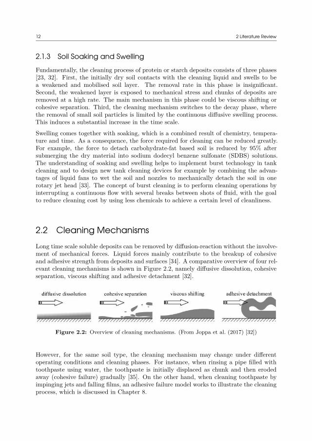
2.2 Cleaning MechanismsLong time scale soluble deposits can be removed by diffusion-reaction without the involve-ment of mechanical forces. Liquid forces mainly contribute to the breakup of cohesiveand adhesive strength from deposits and surfaces [34]. A comparative overview of four rel-evant cleaning mechanisms is shown in Figure 2.2, namely diffusive dissolution, cohesiveseparation, viscous shifting and adhesive detachment [32].
Figure 2.2: Overview of cleaning mechanisms. (From Joppa et al. (2017) [32])
However, for the same soil type, the cleaning mechanism may change under differentoperating conditions and cleaning phases. For instance, when rinsing a pipe filled withtoothpaste using water, the toothpaste is initially displaced as chunk and then erodedaway (cohesive failure) gradually [35]. On the other hand, when cleaning toothpaste byimpinging jets and falling films, an adhesive failure model works to illustrate the cleaningprocess, which is discussed in Chapter 8.
2.3 The Effects of Cleaning Parameters 13
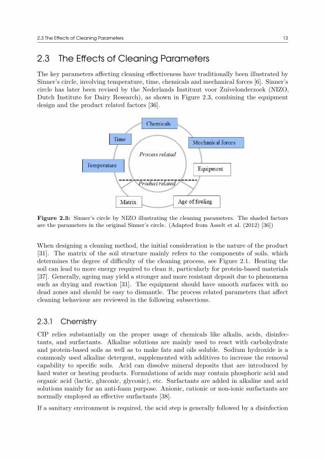
2.3 The Effects of Cleaning ParametersThe key parameters affecting cleaning effectiveness have traditionally been illustrated bySinner’s circle, involving temperature, time, chemicals and mechanical forces [6]. Sinner’scircle has later been revised by the Nederlands Instituut voor Zuivelonderzoek (NIZO,Dutch Institute for Dairy Research), as shown in Figure 2.3, combining the equipmentdesign and the product related factors [36].
Figure 2.3: Sinner’s circle by NIZO illustrating the cleaning parameters. The shaded factorsare the parameters in the original Sinner’s circle. (Adapted from Asselt et al. (2012) [36])
When designing a cleaning method, the initial consideration is the nature of the product[31]. The matrix of the soil structure mainly refers to the components of soils, whichdetermines the degree of difficulty of the cleaning process, see Figure 2.1. Heating thesoil can lead to more energy required to clean it, particularly for protein-based materials[37]. Generally, ageing may yield a stronger and more resistant deposit due to phenomenasuch as drying and reaction [31]. The equipment should have smooth surfaces with nodead zones and should be easy to dismantle. The process related parameters that affectcleaning behaviour are reviewed in the following subsections.
2.3.1 ChemistryCIP relies substantially on the proper usage of chemicals like alkalis, acids, disinfec-tants, and surfactants. Alkaline solutions are mainly used to react with carbohydrateand protein-based soils as well as to make fats and oils soluble. Sodium hydroxide is acommonly used alkaline detergent, supplemented with additives to increase the removalcapability to specific soils. Acid can dissolve mineral deposits that are introduced byhard water or heating products. Formulations of acids may contain phosphoric acid andorganic acid (lactic, gluconic, glyconic), etc. Surfactants are added in alkaline and acidsolutions mainly for an anti-foam purpose. Anionic, cationic or non-ionic surfactants arenormally employed as effective surfactants [38].
If a sanitary environment is required, the acid step is generally followed by a disinfection
14 2 Literature Review
treatment to kill microorganisms or decrease the number of microbes to a safe level.The common disinfection methods include heating, oxidising solutions (e.g., chlorine-based, iodophors, and peroxide-based) and non-oxidising surfactant-based solutions (e.g.,quaternary ammonium compounds, acid anionic, amphoteric disinfectants) [6]. Hydrogenperoxide is a suitable candidate for industrial purposes because the remaining disinfectantcan easily break down into water and oxygen.
Generally, a higher detergent concentration contributes to a higher cleaning rate. How-ever, an optimal detergent concentration may exist for specific soil materials. The increasein chemical concentration above the optimum can only result in limited improvement ofthe cleaning efficiency, sometimes even decreased efficiency. For example, Bird et al.(1991, 1992) indicated the existence of an optimal concentration of NaOH (ca. 0.5 wt%)to clean cooked whey protein [16, 17]. They explained that high alkali concentrationschanged the deposit structure rapidly to form a very thick translucent layer, which wasdifficult to remove. A negative performance by increasing alkaline concentration has alsobeen observed when studying other protein- and lipid-based soils like egg yolk [39], andwas also found in the study reported in Chapter 6.
2.3.2 TemperatureEven though it is often expected to perform cleaning at room temperature, some indus-tries apply heating to increase the cleaning rate and to remove harsh deposits. Using hightemperature in a cleaning process should be thoroughly considered along with the chem-ical effectiveness, system complexity, operating cost and risk, etc. Heating the cleaningmedia and maintaining them at a certain temperature level is one of the biggest energyconsuming steps in a cleaning process [40].
Higher media temperature can increase the diffusion rate of chemicals and the reactionrate, henceforth improve the chemical effectiveness. For example, pink guava puree foulingcannot be effectively cleaned at 35 °C even with high NaOH concentration (up to 2.0wt%). However, when the temperature is increased to 50 °C or 70 °C, fouling is removedcompletely [41]. For yeast soil, an increase in temperature from 30 to 50 °C does notdecrease the cleaning time. However, chemical cleaning at 70 °C can shorten the cleaningtime greatly [42].
An extremely high temperature may sometimes make the cleaning unprofitable. For in-stance, changing water temperature from 22 to 45 °C can improve the rinsing effectivenesssignificantly when flushing reconstituted skim milk from stainless steel pipes. A furtherincrease to 67 °C only improves the cleaning rate slightly but increase the operating costhugely [43]. Furthermore, the increase in temperature can change the structure of de-posits. Goode et al. (2013) found that the dependence of adhesive force on temperaturewas related to the types of deposits and surfaces. For whey protein concentrate deposits,the adhesive force became high after being heated to a temperature above 70 °C dueto the denaturation of proteins. On the contrary, caramel deposits turned to be lessadhesive to stainless steel surfaces with temperature increasing from 30 to 90 °C [44].
Another application of heating is to disinfect surfaces. For example, in the dairy industry,

2.3 The Effects of Cleaning Parameters 15
high temperature is often used after caustic and acid treatments to kill microorganismsor decrease the microbe amount to a safe level.
2.3.3 TimeCleaning time is usually regarded as a characteristic to evaluate the performance of acleaning recipe. In a cleaning practice, the cleaning time is generally determined byassuming that the area that is the most difficult to clean can still be cleaned, which iscalled the “worst case” scenario. In most cases, a long cleaning time results in bettercleaning results. The exceptions are the cases where soil materials become restructuredto be harsher under extreme chemical and heating conditions, like the denaturation ofproteins. However, longer cleaning time also means more resource consumption.
For industrial cleaning operations, a short cleaning time is normally associated with highcleaning efficiency. This is because industries expect a minimized cleaning downtimein order to produce more products in a fixed period. It is estimated that a food andbeverage plant spends approximately 20% of each day on cleaning the equipment. A 20%reduction in cleaning time therefore delivers approximately an extra hour of productiontime to each day [4].
2.3.4 Mechanical ForceThe mechanical force, normally referring to the physical impact that acts on soil layers,is mainly discussed in the cleaning of pipe or pipe-like (e.g., flow cells) systems. Thegeneral rule is that high flow rates lead to high removal rates because of the high impactand shear force on the deposit layer. A critical wall shear stress of 3 Pa is used for thestandardised EHEDG cleaning test method [45].
Asteriadou et al. (2009) coated sweet condensed milk on a lab scale stainless steel couponand fit the soiled coupon in a flow cell. The test coupon was flushed with water. It hasbeen found that the cleaning time decreases greatly by increasing the Reynolds numberfrom 2,500 to 15,000. Interestingly, a further increase only results in a limited reductionof the cleaning time [46]. Gillham et al. (1999) investigated the contribution of eachcleaning factor in different cleaning phases of whey protein concentrate deposits by usingalkaline solutions. They found that the protein removal rate was strongly dependant onthe swelling of the deposit layer in the beginning while the decay phase was more sensitiveto the flow rate (or the wall shear stress) [47].
2.3.5 CoverageIn tank cleaning operations, coverage is related to the total flow of the cleaning liquidbut also related to the selection of the particular tank cleaning device (see Section 2.5.1).The coverage of internal surfaces includes: (1) direct coverage, which is the result of thejets or fans of cleaning liquid hitting the surface to be cleaned directly, and (2) indirectcoverage, which is provided either by a splash-back effect or by the effect of a falling film
16 2 Literature Review
[6]. Coverage is the prerequisite of other parameters like chemistry, temperature, timeand mechanical force.
The coverage of tank surface is dependent on the cleaning time and flow rate. In burstcleaning operations, the period of each burst should ensure that the whole internal surfaceis covered after each cycle. A fast coverage of the tank surface enables fast wetting ofsoil layers. As a result, the cleaning costs are potentially reduced by minimizing chemicalconsumption [33].
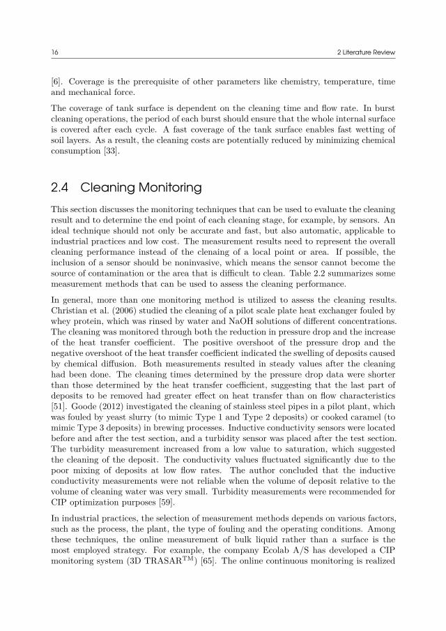
2.4 Cleaning MonitoringThis section discusses the monitoring techniques that can be used to evaluate the cleaningresult and to determine the end point of each cleaning stage, for example, by sensors. Anideal technique should not only be accurate and fast, but also automatic, applicable toindustrial practices and low cost. The measurement results need to represent the overallcleaning performance instead of the clenaing of a local point or area. If possible, theinclusion of a sensor should be noninvasive, which means the sensor cannot become thesource of contamination or the area that is difficult to clean. Table 2.2 summarizes somemeasurement methods that can be used to assess the cleaning performance.
In general, more than one monitoring method is utilized to assess the cleaning results.Christian et al. (2006) studied the cleaning of a pilot scale plate heat exchanger fouled bywhey protein, which was rinsed by water and NaOH solutions of different concentrations.The cleaning was monitored through both the reduction in pressure drop and the increaseof the heat transfer coefficient. The positive overshoot of the pressure drop and thenegative overshoot of the heat transfer coefficient indicated the swelling of deposits causedby chemical diffusion. Both measurements resulted in steady values after the cleaninghad been done. The cleaning times determined by the pressure drop data were shorterthan those determined by the heat transfer coefficient, suggesting that the last part ofdeposits to be removed had greater effect on heat transfer than on flow characteristics[51]. Goode (2012) investigated the cleaning of stainless steel pipes in a pilot plant, whichwas fouled by yeast slurry (to mimic Type 1 and Type 2 deposits) or cooked caramel (tomimic Type 3 deposits) in brewing processes. Inductive conductivity sensors were locatedbefore and after the test section, and a turbidity sensor was placed after the test section.The turbidity measurement increased from a low value to saturation, which suggestedthe cleaning of the deposit. The conductivity values fluctuated significantly due to thepoor mixing of deposits at low flow rates. The author concluded that the inductiveconductivity measurements were not reliable when the volume of deposit relative to thevolume of cleaning water was very small. Turbidity measurements were recommended forCIP optimization purposes [59].
In industrial practices, the selection of measurement methods depends on various factors,such as the process, the plant, the type of fouling and the operating conditions. Amongthese techniques, the online measurement of bulk liquid rather than a surface is themost employed strategy. For example, the company Ecolab A/S has developed a CIPmonitoring system (3D TRASARTM) [65]. The online continuous monitoring is realized
2.4 Cleaning Monitoring 17T
able
2.2:
Mon
itorin
gte
chni
ques
for
foul
ing
and
clea
ning
inC
IPsy
stem
s.(A
fter
Wils
on(2
005)
[31]
)
Met
hods
and
Ref
eren
ces
Mea
surin
gT
imes
cale
Issu
es
Visu
aliz
atio
n[3
7,48
,49
]Lo
calc
onta
min
ated
surfa
ceR
eal-t
ime
orR
etro
spec
-tiv
e
Easy
todo
;Rap
id;S
ubje
ctiv
eas
sess
men
t;A
ccur
acy
and
reso
lutio
n;Tr
aini
ngan
dco
st;N
on-q
uant
itativ
e;H
ard
for
larg
esc
ale
Ove
rall
pres
sure
drop
[ 50,
51]
Hyd
raul
icpe
rform
ance
acro
ssth
eco
ntam
inat
edse
ctio
nR
eal-t
ime
Acc
urac
y(d
iffer
entia
lpre
ssur
e);I
nter
pret
atio
nfo
rco
mpl
icat
edun
its;D
epen
dent
onflo
wpa
tter
n
Ove
rall
heat
tran
sfer
coeffi
cien
t[4
6,50
,51]
The
rmal
perfo
rman
ceof
cont
amin
ated
area
Rea
l-tim
eA
ccur
acy;
Inte
rpre
tatio
n;D
epen
dent
onpr
oces
sm
odel
Loca
lhea
tflu
x[5
2]T
herm
alpe
rform
ance
oflo
calc
onta
min
ated
area
Rea
l-tim
eR
elia
bilit
y;Lo
cal-s
cale
up;M
ater
ialm
odel
ATP
biol
umin
esce
nce
[53,
54]
Mic
robi
olog
ical
activ
ityon
cont
act
surfa
ceor
inliq
uid
Ret
rosp
ectiv
eT
ime
lag;
Spec
ifici
tyof
dete
ctio
n;D
orm
ant
cells
Mic
robi
olog
ical
coun
ting
[53,
55,5
6]M
icro
biol
ogic
alac
tivity
onco
ntac
tsu
rface
Ret
rosp
ectiv
eSo
lubl
ean
din
solu
ble
mat
eria
lson
surfa
ces;
Tim
ela
gan
dtim
eco
nsum
ing;
Skill
edop
erat
ors;
Inva
sive;
Sam
ple
loca
tion
Prot
ein
conc
entr
atio
n[5
7]Fo
ulan
tsin
disa
ssem
bled
pipe
sect
ions
Ret
rosp
ectiv
eIn
vasiv
e;T
ime
lag
and
time
cons
umin
g;C
ompl
exdi
sass
embl
yan
das
sem
bly
Con
duct
ivity
,pH
,or
Turb
idity
[58,
59,6
0,61
]
Foul
ants
and
chem
ical
sin
bulk
liqui
dR
eal-t
ime
Che
ap;R
apid
;Sen
sitiv
ityva
ries
for
diffe
rent
cont
amin
ants
;Bul
kliq
uid
dete
ctio
nso
unce
rtai
nty
ishi
gh;S
peci
ficity
TO
C[6
2]O
rgan
icfo
ulan
tsin
bulk
liqui
dR
eal-t
ime
Sens
itivi
ty;B
ulk
liqui
dde
tect
ion
soun
cert
aint
yis
high
;Tol
eran
ceof
TO
Can
alyz
er;R
equi
resh
ort
resid
ence
time
inth
ean
alyz
er
CO
D[6
1]Fo
ulan
tsan
dch
emic
als
inbu
lkliq
uid
Ret
rosp
ectiv
eBu
lkliq
uid
dete
ctio
nso
unce
rtai
nty
ishi
gh;
Spec
ifici
tyof
foul
ant
Ultr
ason
ics
[63]
Foul
ant
thick
ness
onco
ntam
inat
edsu
rface
Rea
l-tim
eLo
cal;
Har
dfo
rsc
ale-
up;I
ntru
sion
into
flow
;C
alib
ratio
nfo
rfo
ulan
ts
ERT
[64]
Foul
ants
and
chem
ical
sin
bulk
liqui
dR
eal-t
ime
Non
invi
sive;
2Dvi
sual
izat
ion;
Size
ofcr
oss
sect
ion;
Sens
itivi
tyva
ries
for
diffe
rent
foul
ants
;Bul
kliq
uid
dete
ctio
nso
unce
rtai
nty
ishi
gh;S
peci
ficity
18 2 Literature Review
through measuring the temperature, time, flow rate, pH, and turbidity, etc. The turbiditymeasurement controls the quality of cleaning. The other measurements are measuring theprocessing parameters in cleaning cycles. A similar CIP optimization approach, calledOptiCIP, has also been proposed by NIZO [66]. Offline measurements are only applied forstand-alone systems. Conductivity probes have also been installed at present commercialCIP plants [54]. Using such probes, it is possible to monitor the blending phase betweencleaning detergents and rinsing water. The challenge of conductivity analysis is the twodistinctly different conductivity ranges of detergent solutions (acid or caustic) and water.Typically, two sensors with different conductivity ranges are required. Recently, a singlemulti-channel analyser with multi-range measurement capabilities or a single sensor withthe full dynamic range from low to high has been applied [67].
The measurement of adenosine triphosphate (ATP) has also been more and more popularfor cleaning verification, because it directly determines the biological cleaning/contami-nation. ATP is the chemical compound in which energy is stored in all living cells. Itis also present in most food debris. Some quick methods to test the presence of ATPhave been developed, for example by using the enzyme luciferase that emits light when incontact with ATP. The level of luminescence can be measured easily, displaying the pres-ence of living organisms or food debris [44, 54]. Despite its offline manipulation, ATPmeasurements have proven to be an efficient and effective approach to assess cleaningresults when used in combination with other techniques.
2.5 Cleaning Tank Surface and Open Surface
2.5.1 Tank Cleaning DevicesTank cleaning is one of the most common CIP operations in food industries and accom-plished with the help of tank cleaning devices. The purpose of installing a cleaning deviceis to distribute liquid on the tank surface. There are three main choices for tank cleaningtasks, as illustrated in Table 2.3.
A static cleaning head like a static spray ball (SSB) sprays large volumes of low-pressureliquid onto the tank surface at fixed spots. A single axis rotary spray head (RSH) dis-tributes the cleaning liquid using a rotating fan. A rotary jet head (RJH) distributes thecleaning liquid through a number of nozzles, which rotate around both the vertical andhorizontal axes to ensure full coverage of the tank surface. The comparison of these threecleaning devices is described in Table 2.3.
2.5.2 Cleaning by Impinging JetsWater jet flows are extensively used for the removal of deposits from surfaces for exampleby static spray balls and rotary jet heads. When jet flows travel in air, cylindricaljets tend to break into small drops after a certain distance due to air entrainment thatcauses flow instability [68]. The critical distance, where the jet starts to break up, isdetermined by the nozzle diameter, flow velocity, liquid properties, etc. [69]. This jet

2.5 Cleaning Tank Surface and Open Surface 19
Table 2.3: Comparison of typical tank cleaning devices. The images are obtained from onlinesources.
Devices Static spray ball Rotary spray head Rotary jet head
Image
Rotation No rotation Single axis rotation Two-axis rotation
Method Cleaning by spotand falling film
Cleaning by fans ofwater
Cleaning byhigh-impact jets
Mechanicalimpact Low Middle High
Flow rate High Middle LowOperating costs High Middle Low
Applications
Low initial cost;Limited hygiene
requirement; Smalltank size; Weak soil
Low operating cost;Good hygiene
requirement; Smalltank size; Weak soil
Low operating cost;High hygiene
requirement; Largetank size; Harsh soil
breakup phenomenon can happen at both low and high flow velocities (Figure 2.4). Ithas been found that jet breakup promotes cleaning by enlarging the pressurised area [70,71]. However, the impact of a water jet decreases after a certain throw length, leading toreduced cleaning performance. Therefore, an understanding of the stability of liquid jetsis of importance in the design of devices and the optimization of operations in order toremove the largest quantity of deposits with minimized water consumption.
Figure 2.4: Anatomy of water jet breakup in air: (A) Laminar jet, (B) Turbulent jet. (Adaptedfrom Grant et al. (1966) [69])
Wilson et al. (2012), Bhagat et al. (2016) and Chee et al. (2018) studied the flow patternsof liquid from static or moving impinging jets on flat or curved surfaces in pilot scale [72,
20 2 Literature Review
73, 74]. Numerical solutions could be used to describe the velocity profiles on flat surfaceswith different inclination angles. An adhesive removal model was further developed todescribe the cleaning radius of different soil types (soft, intermediate and hard) as afunction of the cleaning time, based on a momentum balance between liquid and depositat the cleaning front [75, 76, 77]. However, this model neglected the effect of jet breakupat long distance and flow splash-back at high flow rate. Therefore, a discrepancy betweenthe predicted cleaning radius and experimental results was found when applying themodel in large scale [78].
The splash-back of liquid occurs at high flow rates, where the liquid expels a shower ofdroplets from the liquid film formed on the surface [79]. It becomes significant when thejet Reynolds number is above 12,000 [80]. On the one hand, splash-back can help withthe indirect coverage within a tank. On the other hand, it reduces the impact at thepoint where the jet impacts directly [6]. The ratio of splashed flow rate to the incomingflow rate is dependent on the jet velocity, jet distance to the surface, nozzle diameter aswell as liquid properties (liquid density and surface tension) [79]. One way to deal withliquid splash-back is to use an effective flow rate term to predict the cleaning performancerather than the actual flow rate [78].
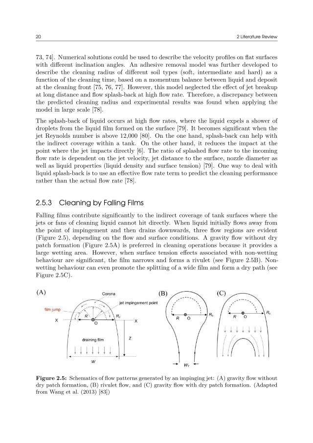
2.5.3 Cleaning by Falling FilmsFalling films contribute significantly to the indirect coverage of tank surfaces where thejets or fans of cleaning liquid cannot hit directly. When liquid initially flows away fromthe point of impingement and then drains downwards, three flow regions are evident(Figure 2.5), depending on the flow and surface conditions. A gravity flow without drypatch formation (Figure 2.5A) is preferred in cleaning operations because it provides alarge wetting area. However, when surface tension effects associated with non-wettingbehaviour are significant, the film narrows and forms a rivulet (see Figure 2.5B). Non-wetting behaviour can even promote the splitting of a wide film and form a dry path (seeFigure 2.5C).
Figure 2.5: Schematics of flow patterns generated by an impinging jet: (A) gravity flow withoutdry patch formation, (B) rivulet flow, and (C) gravity flow with dry patch formation. (Adaptedfrom Wang et al. (2013) [83])
2.6 Mathematical Modelling and Data Analysis 21
The wetting rate, Γ [kg m-1 s-1], is defined to quantify the peripheral flow rate by Γ =m/W , where m is the mass flow rate and W is the wetted width. Hartley et al. (1964)presented the criteria for initiating a dry patch on a vertical surface based on both forcebalance and energy balance theories at the break-point [81]. This threshold depends onthe liquid density (ρ), dynamic viscosity (µ), surface tension (γ), and the contact angle(β) which is a property of the liquid/surface interaction. This criterion can be used tocalculate the minimum wetting rate (Γmin) required to maintain a wide film of liquid forcleaning purposes, see Equation 2.1. Morison et al. (2002) investigated the falling filmson acrylic and stainless steel surfaces generated by a static spray ball, and estimated thatthe minimum wetting rate ranged from 0.1 to 0.3 kg m-1 s-1 [82].
Γ = m/W ≥ 1.69(µρ/g)0.2[γ(1 − cos β)]0.6 = Γmin 2.1
Nusselt (1916) first presented the important film flow theory, assuming that the filmsurface is flat and the flow is truly laminar [84]. However, it has been shown that theliquid may produce a wave motion at extremely low flow rates and within the viscousflow region [85]. A wall shear stress maximum was found to be located either in front ofthe wave crest or behind it [86]. For cleaning operations, a large wall shear stress favoursdeposit removal by shearing the deposit layers. It is of great importance to quantify thethickness and velocity profile of the film as well as the wall shear stress caused by thefilm.
Fuchs et al. (2015, 2013) measured the film thickness using a fluorescence method andfound that the film thickness was strongly affected by the inclination angle of the surface,which, hence, had a major impact on the wall shear stress and the cleaning rate [87, 88].Aouad et al. (2016) measured the surface velocity of draining film generated by liquidjets using particle image velocimetry (PIV) , and revised a model to predict the filmvelocity in the central part of the film [89]. The level of wall shear stress could also bedetermined directly for example by using a dual electrodiffusion friction probe system[90]. Furthermore, it has been found that the stream-wise velocity is strongly disturbedby the presence of an obstacle on the surface like a small deposit [91].
2.6 Mathematical Modelling and Data AnalysisIn the past decades, a number of experiments and models have been made to under-stand how cleaning occurs. The objectives for constructing models are to optimize theequipment design and control variables and to predict the end point of cleaning, which fur-ther result in significant reduction in environmental impact of cleaning operations. Moststudies focus on predictive mathematical models and advanced Computational Fluid Dy-namics (CFD) models. The predictive models are efficient for cleaning practices relatedto monitoring and control purposes. The great computational demand of CFD limits itsapplication for real-time monitoring and control. But it has proven to be a powerful toolfor understanding and improving cleaning processes and equipment design. Since all ofthe systems should be controlled without the occurrence of errors, a risk analysis modelis also introduced here to improve the reliability and safety of operations.
22 2 Literature Review
2.6.1 Predictive Models
2.6.1.1 Response Surface Methodology
The response surface methodology (RSM) approach investigates the functional relation-ship between a response of interest, y, and a series of input variables denoted by x1, x1,...,xk [92]. The most commonly used RSM is the second-order model:
y = β0 +k∑
i=1βixi +
k∑i=1
k∑j=i+1
βijxixj +k∑
i=1βiixii
2 + ϵ 2.2
where y is the estimated response of interest (e.g., cleaning cost and soil removal percent-age); xi is the input variables (e.g., temperature, flow rate, time); β0 is the average valueof the response at the center point; βi,βj ,βij are the coefficients of the linear, interactionand quadratic terms; and ϵ is the statistical error. The regression coefficients for thevariables are obtained by fitting the experimental data. The significance of the modelcan be analysed using an analysis of variance.
The effects of cleaning water temperature and flow rate on the cleaning time, energy andwater consumptions were studied by RSM in the removal of toothpaste from a pilot plantpipe [1]. The flow rate had considerable effects on the cleaning performance. However, theinfluence of temperature was initially little and increased afterwards. The CIP protocolwas optimized based on the model. The cleaning time and the amount of waste waterwere reduced by 53% and 50%, respectively. In another study of the removal of biofilmfrom a chilling tank, the log reduction in biofilm cells was characterized as response.The input variables were cleaning time, temperature and NaOH concentration [55]. Anoptimized CIP regime was achieved: 1.5 wt% NaOH at 65 °C for 30 min −→ water rinse−→ 1 wt% HNO3 at 65 °C for 10 min −→ water rinse. The optimized CIP resulted in a4.77 log reduction in biofilm cell count, compared with a 3.29 log reduction in biofilm cellcount in the reference CIP. Jurado Alameda et al. (2016) used the RSM to investigate thecleaning of starch films using nonionic and zwitterionic surfactant solutions [93]. Similarto RSM, Piepiórka-Stepuk et al. (2016) defined a cleaning degree factor and an energyconsumption factor, and correlated them with temperature, flow rate and cleaning time.These two factors were introduced as a new multicriterial function to find the optimaloperating conditions with high cleaning efficiency and low energy input [94].
RSM is a useful method to evaluate the effects of different variables and their interactionsfrom the minimum number of experiments. It is very effective to model and optimizeCIP operations. The design of experiments is very important in any RSM investigation,because the choice of the variable matrix needs to be representative.
2.6.1.2 Function Fitting Models
One aim of predictive models is to predict the end point variation of cleaning. One of themost common predictive models is based on the functional form, which uses the cleaningdata collected from an ongoing operation to predict the future cleaning behaviour whencleaning has commenced. For example, the existing removal curve of toothpaste can be
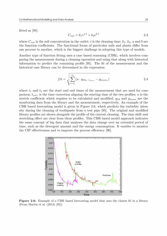
2.6 Mathematical Modelling and Data Analysis 23
fitted as [95]:Cout = k1ea·t + k2eb·t 2.3
where Cout is the soil concentration in the outlet; t is the cleaning time; k1, k2, a and b arethe function coefficients. The functional forms of particular soils and plants differ fromone process to another, which is the biggest challenge in adopting this type of models.
Another type of function fitting uses a case based reasoning (CBR), which involves com-paring the measurement during a cleaning operation and using that along with historicalinformation to predict the remaining profile [95]. The fit of the measurement and thehistorical case library can be determined in the expression:
fit =
√√√√ t2∑i=t1
(n · ylibi−tcorr− ymeasi
) 2.4
where t1 and t2 are the start and end times of the measurement that are used for com-parison; tcorr is the time correction aligning the starting time of the two profiles; n is thestretch coefficient which requires to be calculated and modified; ylib and ymeas are themonitoring data from the library and the measurement, respectively. An example of theCBR based forecasting model is given in Figure 2.6, which predicts the turbidity inten-sity during the cleaning of toothpaste from a test pipe [95]. The original and modifiedlibrary profiles are shown alongside the profile of the current cleaning. The time shift andstretching effect are clear from these profiles. This CBR based model approach indicatesthe same concept of big data that analyses the data change over an extended period oftime, such as the detergent amount and the energy consumption. It enables to monitorthe CIP effectiveness and to improve the process efficiency [96].
Figure 2.6: Example of a CBR based forecasting model that uses the closest fit in a library.(From Martin et al. (2013) [95])

24 2 Literature Review
2.6.1.3 Mechanism-Based Models
In the aforementioned function based forecasting models, the functions are obtained byfitting the current curve, which may be meaningless to describe how the cleaning oc-curs. Another type of model is based on a mechanism, which tries to explain the process.For example, a hybrid model with a simple mechanistic structure and empirical kineticsdescribed the cleaning of whey protein, based on the assumption that the cleaning in-volved the top swollen layer removal and the residual soil removal. The model could berepresented as Equation 2.5 [16, 97]:
dlsdt
= Rs − Rr, Rs = a − b · ls,dlrdt
= Rr = k · ls, F = Rτ · ρsoil 2.5
with initial conditions ls(0) = 0, lr(0) = L. ls and lr are the thickness of the swollen layerand the residual soil; Rs and Rr are the rate of change of these two layers; a, b and kare the constants related to the cleaning kinetics; ρsoil is the density of the removed soil;F is the mass rate of the removed soil; and L is the initial thickness of the soil prior tocleaning. This model includes the forecasting concept as well.
A cleaning model can be derived based on different cleaning steps as well. For example,in the cleaning of milk systems, the total remaining deposit can be expressed as [98]:
mT OT (t) = mW AT (t) + mALK(t) + mACD(t) + mRES(t) 2.6
where mT OT (t) is the total remaining mass at any time t in the CIP process; mW AT (t) isthe deposit removed by warm water rinsing; mALK(t) is the deposit removed by alkalinewashing; mACID(t) is the deposit removed by acid washing; and mRES(t) is the residualamount at time t. Each step includes a fast removal rate of the tightly bonded depositand a slow removal rate of the loosely bonded deposit. For example, the removal rate inthe warm water rinsing step can be written as follows:
dmW AT,F (t)dt
= −kW AT,F · mW AT,F (t)
dmW AT,S(t)dt
= −kW AT,S · mW AT,S(t)2.7
where mW AT,F (t) and mW AT,S(t) are the fast and slow removal rate, respectively. Thecoefficients kW AT,F and kW AT,S are correlated to the experimental results. Similar func-tions also apply to the alkaline rinsing and acid rinsing steps. The mechanistic modelsare difficult to construct, as they require deeper understanding of the process. But theyare very useful to make efficient cleaning strategies.
2.6.1.4 Kinetics-Based Models
Another type of forecasting models with physical meaning that are constructed is thekinetics-based model. An example is demonstrated from the removal of Bacillus cereusstrains from pipes rinsed by a NaOH solution [99]. This work assumes that removal anddeposition occur at the same time, applying the pseudo-first-order models. The removalpart can be expressed as:
dN(t)dt
= k1(N(t) − NR) 2.8
2.6 Mathematical Modelling and Data Analysis 25
and the deposition of spores can be expressed as:dN(t)
dt= k2(N0 − N(t)) 2.9
where N(t), NR and N0 are the surface density of adhering spores at time t, at infinite timeand at initial time, respectively; k1 and k2 are model coefficients, representing constantsof removal and deposition, respectively. The value of k2 is related to the total area ofcontamination and the detergent volume. The removal and deposition occur concurrently.Then the equations can be associated as follows:
dN(t)dt
= k2(N0 − N(t)) − k1(N(t) − NR) 2.10
This equation can be solved by integrating between time 0 and t. Parameters are identifiedusing experimental values. It is hypothesized that the removal rate constant, k1, becomessmaller if water is used instead of NaOH solution.
2.6.2 Computational Fluid DynamicsThe removal of soils and microorganisms is affected by the local flow conditions (e.g., wallshear stress and its fluctuating rate), detergent mixing, and heat distribution, etc. [56,100]. CFD has become an effective tool to predict these local properties [101]. The mainadvantages of using CFD are that: (1) it is possible to test different designs withoutbuilding prototypes; (2) it is possible to calculate the local properties where measure-ments cannot reach. Therefore, CFD has been carried out in early design works to im-prove hygienic design, showing the effects of wall shear stress and fluctuation on cleaningbehaviour.
Figure 2.7 shows a T-joint with a dead end geometry, which is unwanted but inevitablein food processing lines [102]. Detergents and fluid may be stagnant in these areas dueto low velocity and low wall shear stress, consequently resulting in ineffective cleaningperformance. CFD simulates the distribution of velocity and wall shear stress at differentflow rates. It has been found that an increase in the incoming flow rate can increase localvelocities generally, but the influence on the stagnant area is very small (the blue areasin Figure 2.7B). The fluctuation rate of wall shear stress is linked with the turbulenceintensity, which can be obtained from steady-state simulations as well [101]. Therefore,the CFD results are helpful to improve the hygienic design of equipment by avoidingstagnant zones, and to optimize the operating conditions.
Another application of CFD is to simulate the displacement process of soils. Figure 2.8displays the displacement of yoghurt by water in a dairy pilot line of 60 mm inner diameterat average flow rate of 170 kg/min [64]. Both the measurement and the CFD simulationdescribe a clear tailing effect of yoghurt removal at the lower section of the pipe, whichis caused by the density difference between yoghurt and water. The CFD model can befurther used to investigate the effects of pipe length, water flow rates, yoghurt rheologyand wall slips, as well as yield stress.
CFD has become a valuable supplement to EHEDG tests. It is currently the only alter-native to testing different sizes of the same piece of equipment. For example, CFD has
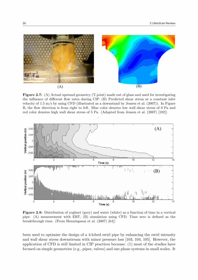
26 2 Literature Review
Figure 2.7: (A) Actual upstand geometry (T-joint) made out of glass and used for investigatingthe influence of different flow rates during CIP. (B) Predicted shear stress at a constant inletvelocity of 1.5 m/s by using CFD (illustrated as a downstand by Jensen et al. (2007)). In FigureB, the flow direction is from right to left. Blue color denotes low wall shear stress of 0 Pa andred color denotes high wall shear stress of 5 Pa. (Adapted from Jensen et al. (2007) [102])
.
Figure 2.8: Distribution of yoghurt (grey) and water (white) as a function of time in a verticalpipe: (A) measurement with ERT, (B) simulation using CFD. Time zero is defined as thebreakthrough time. (From Henningsson et al. (2007) [64])
been used to optimize the design of a 4-lobed swirl pipe by enhancing the swirl intensityand wall shear stress downstream with minor pressure loss [103, 104, 105]. However, theapplication of CFD is still limited in CIP practices because: (1) most of the studies havefocused on simple geometries (e.g., pipes, valves) and one phase systems in small scales. It
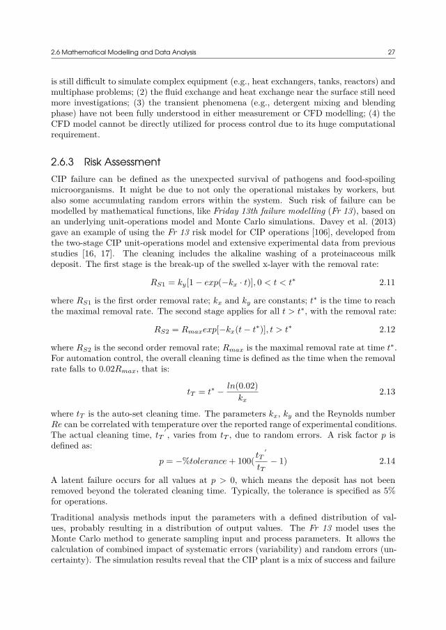
2.6 Mathematical Modelling and Data Analysis 27
is still difficult to simulate complex equipment (e.g., heat exchangers, tanks, reactors) andmultiphase problems; (2) the fluid exchange and heat exchange near the surface still needmore investigations; (3) the transient phenomena (e.g., detergent mixing and blendingphase) have not been fully understood in either measurement or CFD modelling; (4) theCFD model cannot be directly utilized for process control due to its huge computationalrequirement.
2.6.3 Risk AssessmentCIP failure can be defined as the unexpected survival of pathogens and food-spoilingmicroorganisms. It might be due to not only the operational mistakes by workers, butalso some accumulating random errors within the system. Such risk of failure can bemodelled by mathematical functions, like Friday 13th failure modelling (Fr 13), based onan underlying unit-operations model and Monte Carlo simulations. Davey et al. (2013)gave an example of using the Fr 13 risk model for CIP operations [106], developed fromthe two-stage CIP unit-operations model and extensive experimental data from previousstudies [16, 17]. The cleaning includes the alkaline washing of a proteinaceous milkdeposit. The first stage is the break-up of the swelled x-layer with the removal rate:
RS1 = ky[1 − exp(−kx · t)], 0 < t < t∗ 2.11
where RS1 is the first order removal rate; kx and ky are constants; t∗ is the time to reachthe maximal removal rate. The second stage applies for all t > t∗, with the removal rate:
RS2 = Rmaxexp[−kx(t − t∗)], t > t∗ 2.12
where RS2 is the second order removal rate; Rmax is the maximal removal rate at time t∗.For automation control, the overall cleaning time is defined as the time when the removalrate falls to 0.02Rmax, that is:
tT = t∗ − ln(0.02)kx
2.13
where tT is the auto-set cleaning time. The parameters kx, ky and the Reynolds numberRe can be correlated with temperature over the reported range of experimental conditions.The actual cleaning time, tT
′ , varies from tT , due to random errors. A risk factor p isdefined as:
p = −%tolerance + 100( tT′
tT− 1) 2.14
A latent failure occurs for all values at p > 0, which means the deposit has not beenremoved beyond the tolerated cleaning time. Typically, the tolerance is specified as 5%for operations.
Traditional analysis methods input the parameters with a defined distribution of val-ues, probably resulting in a distribution of output values. The Fr 13 model uses theMonte Carlo method to generate sampling input and process parameters. It allows thecalculation of combined impact of systematic errors (variability) and random errors (un-certainty). The simulation results reveal that the CIP plant is a mix of success and failure

28 2 Literature Review
as a result of random system errors. The risks come from not only the auto-set cleaningtime, but also the auto-set cleaning fluid temperature.
Besides the two-stage CIP model, the Fr 13 model can also be used in combinationwith the more complicated three-stage CIP model from Xin (2003, 2004): the swellingof deposit by alkaline, the uniform removal with constant removal rate and the decay[107, 108, 109]. The application of risk analysis helps to assess control and other processintervention strategies and improve the reliability and safety of operations [106, 109].
2.7 ConclusionsSeveral fouling problems and cleaning techniques have been discussed in the scientificliterature. Three soil types have been classified according to the complexity of soil prop-erties and the difficulty of removal. For type 1 soil, it is enough to solely use wateras cleaning media. For type 2 soil, removal needs to be preceded by the destruction ofbiofilm. Type 3 soil is the most reluctant deposit that requires chemicals to remove. Var-ious measurement techniques can be used to study soils in order to (1) understand thecleaning mechanism, (2) measure the required force to remove deposits from surfaces, and(3) measure the internal properties of deposits. These techniques are very helpful to inves-tigate how cleaning occurs at micro scale. Especially, the understanding of soil soakingand swelling may introduce the novel development of burst technique in tank cleaningoperations. Furthermore, four cleaning mechanisms have been proposed to describe acleaning process, namely diffusive dissolution, cohesive separation, viscous shifting, andadhesive detachment. These mechanisms may occur synchronously, depending on soiltypes, cleaning methods and cleaning phases, etc.
The main parameters that determine cleaning results include temperature, time, chem-icals, mechanical forces, surface coverage as well as soil properties like structure matrixand ageing. Generally speaking, higher temperature, higher detergent concentration andhigher mechanical impact are helpful to shorten the cleaning time. However, above sometemperatures, the extra heat may generate more elastic deposits which are even moredifficult to remove. Excessive flow rates and chemical consumption may result in lim-ited improvement of cleaning efficiency, but increase the operating cost significantly. Forsome protein-based soils like whey protein and egg yolk, an optimal alkali concentrationis observed, above which the soil layers become less penetrable to the cleaning agent.
Several monitoring techniques have been developed to assess the cleaning results and todetermine the end point of each cleaning stage. The monitoring methods can be eitherreal-time or retrospective. Each method has its own field of application. Among themethods, the measurement of bulk liquid using pH, conductivity and turbidity sensorssurpasses the others due to its applicability in large scale. ATP measurement is anotherremarkable technique for detecting the existence of residual microorganisms and fooddebris.
For the cleaning of tank surfaces, a cleaning device is required to distribute cleaning liquidon the surface with high impact. The coverage of the internal surface can be achievedby either direct hitting of liquid jets or indirect flow by falling films. The cleaning by
2.7 Conclusions 29
impinging jets can be modelled by numerical equations. However, the application of thepresent models needs the consideration of jet breakup and splash-back if proposed forlarge scale. The studies of falling films have been mainly associated with the wetting ratefor a wide film and film characteristics (i.e., thickness, velocity profile, and wall shearstress).
In the end of this chapter, some mathematical modelling and data analysis methods werepresented. Four predictive models are discussed, in regard to predicting the cleaningprofile and possibly a cleaning end point. CFD models are not applicable for real-timemonitoring and control due to their huge computational demand, but they are helpful inthe optimization of operations and equipment design. A CIP operation is less tolerantof a potential failure because any cleaning failure may result in a catastrophic disasterto public health. Therefore, failure analysis of CIP becomes of great importance in thisrespect.

30

Part II
Case Studies

CHAPTER3Mapping CIP Systems in
a Brewery3.1 Introduction
3.1.1 Brewing Process
The purpose of brewing is to produce beer through a series of process steps. As shown inFigure 3.1, the process starts with the milling of raw materials such as barley malt andrice grains. Then these raw materials are mashed into a sugary fermentable liquid calledwort. The wort is boiled with hops added, and cleared to remove solid particles. Next,this liquid medium is converted into an alcoholic, carbonated beverage by yeast, followedby maturation. Afterwards, the matured green beer is filtrated to get bright beer. As aresult of the above process steps, the product is ready to be filled into bottles, cans orkegs, before being shipped to distributors [110].
As indicated in Figure 3.1, a brewing process includes many equipments that need to becleaned after use. For example, the operations prior to fermentation take place in a brewhouse, where there are silos, millers, filters, boilers, heat exchangers, etc. Fermentationand maturation generally occur in either a vertical cylinder with a conical bottom ora horizontal tank. In a packaging plant, beer containers and crates should be cleanedbefore filling with beer. In addition, shipment vehicles like trucks need to be washed aswell. There are still cleaning operations that are not indicated in Figure 3.1, such as thecleaning of pipes, pumps, valves, as well as water purification systems.
Most of the cleaning operations in large scale breweries can be accomplished throughautomated CIP recipes by installing several CIP systems to clean different equipmentsor processes. Though, manual cleaning and cleaning-out-of-place (COP, to dismantlea device and wash it separately) operations are still used for other parts. Small scalebreweries may choose movable CIP stations to clean small facilities one by one ratherthan a big and fixed CIP system. However, soil types and cleaning cycles are similarfrom small scale to large scale.
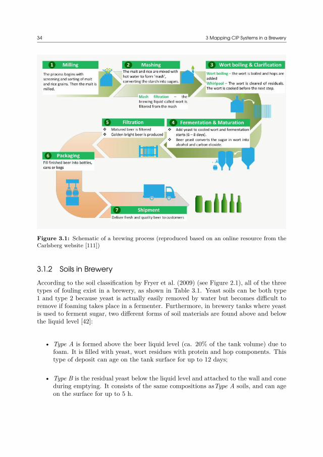
34 3 Mapping CIP Systems in a Brewery
Figure 3.1: Schematic of a brewing process (reproduced based on an online resource from theCarlsberg website [111])
3.1.2 Soils in BreweryAccording to the soil classification by Fryer et al. (2009) (see Figure 2.1), all of the threetypes of fouling exist in a brewery, as shown in Table 3.1. Yeast soils can be both type1 and type 2 because yeast is actually easily removed by water but becomes difficult toremove if foaming takes place in a fermenter. Furthermore, in brewery tanks where yeastis used to ferment sugar, two different forms of soil materials are found above and belowthe liquid level [42]:
• Type A is formed above the beer liquid level (ca. 20% of the tank volume) due tofoam. It is filled with yeast, wort residues with protein and hop components. Thistype of deposit can age on the tank surface for up to 12 days;
• Type B is the residual yeast below the liquid level and attached to the wall and coneduring emptying. It consists of the same compositions asType A soils, and can ageon the surface for up to 5 h.
3.2 Methods 35
Table 3.1: Different fouling materials and fouling types in a brewery (adapted from Goode(2012) [59])
Plant geometries Fouling materials Fouling typesWort boilers Protein, beer stone Type 3
Fermenters and maturation tanks Yeast protein, slight beer stone Type 2Yeast storage tanks Yeast protein, slight beer stone Type 1
Bright beer storage tanks Traces of beer and foam Type 1
3.1.3 Purpose of Mapping in Carlsberg Danmark A/SCarlsberg Danmark A/S is a global brewer with the headquarter located in Copenhagen,Denmark. The Carlsberg brewery in Fredericia is one of the main production sites toproduce beer and soft drinks. Mapping of the CIP systems in the Carlsberg brewery inFredericia is the preliminary step in the INNO+DRIP project in order to upgrade theexisting CIP operations.
According to a pre-assessment report about water efficiency in Carlsberg’s Fredericia site,CIP processes (only including part of the CIP systems) are the third largest sink of water,following the water used in the production of soft drinks and beer. Significant potentialshave been identified related to the optimization of CIP operations. The complexity ofCIP systems varies site by site, line by line and unit by unit. Therefore, this mappingcase study is conducted in order to understand the performance of these CIP systemsand to identify potential savings.
However, due to the complexity of the overall process, this mapping study exclusivelyassesses the CIP systems in the brewery plant. To be exact, the results and conclusionsare mainly focusing on the cleaning of tanks (fermenters, storage tanks, etc.) and transferlines (pipes, pumps, valves, etc.). In this thesis chapter, CIP processes and data valuesare not reported for confidentiality reasons. Nevertheless, the findings in this case are veryrepresentative of common industrial CIP practices in other industries like dairy, beverageand pharmaceutical. This case study also provides the factual basis for implementing theresearch projects described in the remaining chapters.
3.2 MethodsThis mapping study was performed through on-site review and data analysis that recordedhistorical cleaning operations. A mapping report was accomplished to document CIPsystems, chemical supplies, cleaning recipes, water and energy consumptions, cleaningfrequencies, measurements and CIP equipment, etc. This thesis only presents examplesabout cleaning time and annual costs, which were calculated according to the aforemen-tioned information through Equation 3.1.
δT otal = δF resh water + δDetergent + δElectricity + δHeat + δW aste water 3.1
36 3 Mapping CIP Systems in a Brewery
The term δ with subscripts denotes the cost of each item. The costs of fresh water,detergent, electricity, sensible heat and waste water treatment were computed as follows:
δF resh water = Q · t · φF resh water 3.2δDetergent = Q · t · C · φDetergent 3.3δElectricity = (Pf + Ps) · t · φElectricity 3.4
δHeat = Q · t · ρ · cP · (T − T0) · φHeat 3.5δW aste water = Q · t · φW aste water 3.6
where Q is the flow rate; t is the cleaning time; C is the detergent concentration; Pf and Ps
are the powers of forward and scavenge pumps; ρ and cP are the density and heat capacityof the liquid; T and T0 are the cleaning temperature and room temperature, respectively.The unit cost of each cleaning resource, φ with subscript (i.e., water, detergent, heatingenergy, electricity, waste water treatment), was based on the prices in Danish industries.If there were recoveries of water or detergent solutions, the costs were reduced by replacingthe flow rate Q as the difference in flow rates between the feeding flow and the recoveryflow, neglecting the dilution effect and reaction loss.
3.3 Mapping Results
3.3.1 A Cleaning ExampleFigure 3.2 displays the cleaning time spent on each step for a typical cleaning example.The current recipe is time-based, meaning that each step is performed for a pre-definedperiod. The times for detergent circulations (alkali, acid and disinfectant) contributeto over 80% of the overall cleaning time. The pre-rinse and intermediate rinse steps aregenerally shorter than the final rinse, which makes sense because the final rinse is essentialin order to remove all residual soils and detergents from the system.
Figure 3.3 shows the cost of each cleaning resource using cleaning times from Figure 3.2and Equations 3.2 to 3.6. It can be seen that nearly 98% of the cleaning costs attributeto detergent solutions, particulary disinfectant and alkaline solutions. Taking a recoveryratio of 95% based on the estimation of the actual processes, the overall cleaning costscan be reduced by ca. 93% through the recovery of detergent solutions. Then, the costsof water (the sum of pre-rinse, intermediate rinses and final rinse) become the secondcontributor to the overall costs besides disinfectant. The costs of electricity and wastewater treatment are very low compared with other factors.
3.3.2 Annual Cleaning CostsThe annual cleaning costs of each process can be calculated as the product of cleaningfrequency per year and costs per cleaning. It is found in Figure 3.4A that ca. 70% ofthe cleaning operations are performed for pipes, because pipes are frequently used for thetransfer of materials, products, yeast, etc. There are two cleaning recipes for fermenters,named CIP of fermenters and disinfection of fermenters, because a cleaned fermenter
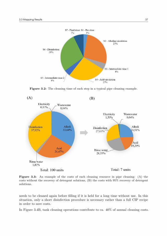
3.3 Mapping Results 37
Figure 3.2: The cleaning time of each step in a typical pipe cleaning example.
Figure 3.3: An example of the costs of each cleaning resource in pipe cleaning: (A) thecosts without the recovery of detergent solutions, (B) the costs with 95% recovery of detergentsolutions.
needs to be cleaned again before filling if it is held for a long time without use. In thissituation, only a short disinfection procedure is necessary rather than a full CIP recipein order to save costs.
In Figure 3.4B, tank cleaning operations contribute to ca. 40% of annual cleaning costs.
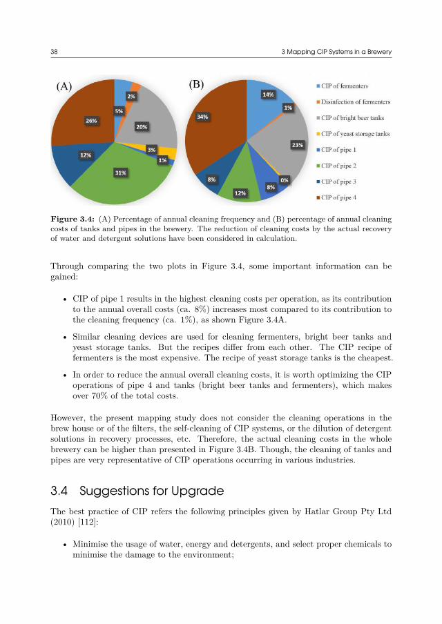
38 3 Mapping CIP Systems in a Brewery
Figure 3.4: (A) Percentage of annual cleaning frequency and (B) percentage of annual cleaningcosts of tanks and pipes in the brewery. The reduction of cleaning costs by the actual recoveryof water and detergent solutions have been considered in calculation.
Through comparing the two plots in Figure 3.4, some important information can begained:
• CIP of pipe 1 results in the highest cleaning costs per operation, as its contributionto the annual overall costs (ca. 8%) increases most compared to its contribution tothe cleaning frequency (ca. 1%), as shown Figure 3.4A.
• Similar cleaning devices are used for cleaning fermenters, bright beer tanks andyeast storage tanks. But the recipes differ from each other. The CIP recipe offermenters is the most expensive. The recipe of yeast storage tanks is the cheapest.
• In order to reduce the annual overall cleaning costs, it is worth optimizing the CIPoperations of pipe 4 and tanks (bright beer tanks and fermenters), which makesover 70% of the total costs.
However, the present mapping study does not consider the cleaning operations in thebrew house or of the filters, the self-cleaning of CIP systems, or the dilution of detergentsolutions in recovery processes, etc. Therefore, the actual cleaning costs in the wholebrewery can be higher than presented in Figure 3.4B. Though, the cleaning of tanks andpipes are very representative of CIP operations occurring in various industries.
3.4 Suggestions for UpgradeThe best practice of CIP refers the following principles given by Hatlar Group Pty Ltd(2010) [112]:
• Minimise the usage of water, energy and detergents, and select proper chemicals tominimise the damage to the environment;
3.4 Suggestions for Upgrade 39
• Operate the CIP systems by ensuring various interface boundaries by instrumenta-tion (pH, conductivity, turbidity, etc.) rather than time or visual inspection;
• Optimise the operating conditions based on need;
• Use single-use systems for small or rarely used equipment or where the cleaningsolutions are grossly contaminated.
According to the CIP best practice guidelines and the need of the industrial CIP user,the improvement of current CIP systems in the mapped brewery can be implemented infive aspects as follows [112], which can also be regarded as reference in other breweriesand other industries:
1. Improve product removal
a) Inspecting the draining capability of the equipment, allowing gravity drainingof the product for recovery;
b) Using turbidity or other forms of measurements to determine whether theproduct has been sufficiently removed rather than time-based;
c) Recovering the product prior to CIP to avoid drying fouling;d) Using carbonated water and product mixture to assist product removal and
recovering the liquid in the product.
2. Minimise rinsing water use
a) Intalling spray devices as close as to the foam part in fermeters, which is themost difficult to remove;
b) Selecting the water of proper quality (“fit-for-use”) and treating the water forapplicable purpose (“fit-for-purpose”), and reusing water from intermediaterinse and final rinse for use in the pre-rinse of next cleaning;
c) Optimising the flow rate and rinsing time and implementing measurement-based rinse instead of time-based.
3. Minimise chemical use
a) Optimising chemical conditions (i.e., concentration, flow rate, temperatureand time), as most cleaning parameters are determined based on experienceswithout examination in specific applications;
b) Using alternative chemicals like potassium hydroxide (KOH) and enzymes inorder to reduce the environmental impact;
c) Holding frequently used chemical solutions at required temperature to shortenthe cleaning time that is spent on raising the temperature prior to CIP;
d) Recovering chemicals at a proper ratio (ca. 80%) to reduce volume loss (ifrecovering too little) and dirt accumulation in the tanks (if recovering toomuch).
40 3 Mapping CIP Systems in a Brewery
4. Improve equipment performance
a) Checking the proper use of cleaning devices and inspecting the dead ends inthe systems;
b) Separately cleaning the equipment difficult to clean, e.g., centrifuges, rotationalparts, and heat exchangers;
c) implementing in-line measurements to monitor the process and determine theend point of cleaning.
5. Other aspects
a) Checking the cleaning recipes of some processes where expensive recipes areused to clean easy soils;
b) Rearranging the orders of detergent tanks so that the earlier used liquid shouldbe closer to the forward pump, in order to avoid cross-contamination in CIPfeeding pipes. For example, if the cleaning recipe is “pre-rinse −→ alkaline−→ acid −→ disinfection −→ final rinse”, the ideal order of CIP tanks shouldbe:(Forward pump - ) Reused water tank - Alkali tank - Acid tank - Disinfectanttank - Fresh water
c) Simplifying the cleaning process by for example combining the disinfectionstep with the acid circulation step to reduce the cleaning time;
d) Implementing a smart production schedule to avoid long holding times of equip-ment and repeated cleaning operations before new productions.
3.5 Inspirations for This Ph.D ThesisThis mapping study has provided a number of possibilities to reduce the annual cleaningcosts in a brewery. This Ph.D thesis is motivated by this case study and aims at providingpractical solutions to upgrade CIP systems and processes using academic knowledge. Fourprojects have been defined in this respect and were organised as follows:
1. For an existing CIP system
a) Analyzing historical data of CIP operations is essential to avoid potential op-eration failures in the future. Chapter 4 presents a three-level approach ofanalysis based on the CIP of a brewery fermenter at Carlsberg to describe howto analyse the historical data in steps for detecting anomalies. The potentialapplication of the analysis approach is to integrate a reference model into thecontrol system for automatically indicating and diagnosing likely anomalousevents;
b) Pipe cleaning is one of the main costs in cleaning operations. Reducing theuse of rinsing water and improving the recovery of detergent solutions canpotentially decrease the operating costs of pipe cleaning. Chapter 5 presents
3.6 Conclusions 41
how CFD tools can be applied to simulate the displacement of detergent solu-tions by water. The purpose is to understand the blending phase within pipesystems and to optimise flow conditions and detergent/water recovery;
2. For designing a new system
a) The costs of alkali are the main costs in the cleaning of fermenters because al-kaline solution is not recovered due to deactivation by CO2. In Chapter 6, theburst technique is investigated in tank cleaning operations and compared withconventional continuous flows. The goal of burst cleaning is to improve the ef-fectiveness of alkali usage and to reduce the detergent consumption henceforthreduce the cleaning costs;
b) The current recovery of cleaning liquid is controlled based on time or conductiv-ity measurements. Chapter 7 develops a measurement-based recovery system.A turbidity sensor is applied to measure the quality of water for switchingbetween water recovery and draining. The goal is to only reuse clear liquidand increase the lifetime of reused water.
3.6 ConclusionsCIP is commonly used in industrial breweries. All of the three fouling types, classifiedaccording to Fryer et al. (2009) [15], exist in different brewing processes. Yeast is themain fouling material in wort boilers, fermenters, yeast and bright beer tanks, as wellas transfer lines. For a beer fermenter, yeast soils above liquid level are more difficultto remove than the soils below liquid level because of foaming. This mapping studyassessed the main CIP systems at the Carlsberg brewery, with special attention paid onthe cleaning of tanks and pipes. This thesis mainly presents the economic evaluation ofcleaning operations.
In general, the CIP systems at Carlsberg are highly automated and efficient. The treat-ment of cleaning detergents (alkali, acid and disinfectant) contributes significantly to theoverall cleaning time and cleaning costs. The recovery of cleaning detergents can reducethe cleaning costs by over 90%. The annual costs of pipe cleaning (ca. 60%) are higherthan the costs of tank cleaning (ca. 40%), because pipe cleaning operations occur morefrequently.
Based on the mapping results, suggestions for implementing the best practice of CIPhave been provided to Carlsberg by improving product removal, minimising rinsing wateruse, minimising chemical use, upgrading equipment, and some other aspects. Thesesuggestions can also be useful to improve the CIP systems in other industries wheresimilar processes are applied.
In the end, based on the mapping study in the brewery case, four projects are definedin this Ph.D thesis. The aim of this thesis is to provide practical solutions to upgradeexisting CIP systems or design new systems.

42 3 Mapping CIP Systems in a Brewery
List of Nomenclature in Chapter 3The following nomenclature is only valid for this chapter. Some symbols are used in otherchapters but with different meanings. Otherwise, the symbols are specifically explainedin the text if there is no nomenclature in some chapter.
Roman LetterscP Heat capacity of liquid, [kg m2 °C-1 s-1]C Detergent concentration, [kg m-3]Pf , Ps Power of feed pump and scavenge pump, [kW]Q Flow rate, [m3 min-1]t Time, [min]T Cleaning temperature, [°C]T0 Room temperature, [°C]
Greek Lettersδ with subscript Cleaning cost (of resource), [Euro]ρ Liquid density, [kg m-3]φ with subscript Unit cost of a cleaning resource, [Euro per unit resource]
CHAPTER4Anomaly Analysis in CIP
Operations of aBrewery Fermenter
In this chapter, the historical data from the cleaning of a brewery fermenter at Carlsberg isanalysed with the purpose to detect anomalies in monitoring and diagnose the potentialcauses. The work was performed in collaboration with Alfa Laval Copenhagen A/S,Carlsberg Danmark A/S and Ecolab Danmark A/S. This chapter of the thesis has beenpublished and reproduced with permission from [113]
Anomaly Analysis in Cleaning-in-Place Operations of an Industrial Brewery FermenterYang, J., Jensen, B. B. B., Nordkvist, M., Rasmussen, P., Pedersen, B., Kokholm, A.,Jensen, L., Gernaey, K. V., Krühne, U.Industrial and Engineering Chemistry Research, 57 (38): 12871 - 12883. (2018)DOI: 10.1021/acs.iecr.8b02417
Copyright 2018 American Chemical Society.
4.1 IntroductionChapter 3 describes a mapping study of CIP systems at the Carlsberg Fredericia brewerysite. There are lots of monitoring data from historical cleaning operations. A potentialapplication of the data is to establish forecasting models to identify the likely future CIPperformance by comparing the current observations with previously stored experiences,as described in Section 2.6.1.2 [95]. Another method to use the data is to evaluateand optimize the system by examining the current parameters or processes manuallyand periodically. For instance, a CIP specialist, sometimes an auditor, can check if thecleaning duration or flow rate is insufficient or over demand by reading the record. Thiskind of analysis is normally conducted by external experts infrequently (e.g., once peryear). Industry anticipates a more efficient and automatic approach to evaluate a cleaningoperation and detect abnormal events right after cleaning or even immediately when itoccurs.
44 4 Anomaly Analysis in CIP Operations of a Brewery Fermenter
In present, the analysis of historical cleaning data is usually experience-based. It isexpected that this fact will remain in the near future. The aforementioned methods touse the data have the aim to investigate only one parameter at once, which is called aunivariate statistical approach [114]. However, in complex processes, a large data set isgenerated, containing many interacting variables. Then, multivariate methods becomeessential, allowing monitoring and analysing multiple variables simultaneously [115].
In this chapter, the introduced three-level approach to analyse CIP monitoring dataapplies both univariate and multivariate approaches. The aim is to benchmark how touse historical cleaning data to evaluate anomalies occurring in CIP, by taking an examplefrom the cleaning of a brewery fermenter.
4.2 Description of the CIP Practice of a BreweryFermenter
The proposed analysis benchmark was based on the cleaning of a 500 m3 brewery fer-menter at Carsberg’s Fredericia site. The vertical fermenter, mainly soiled by yeast, wascleaned with help of a rotary jet head (Alfa Laval, Denmark). There were 27 CIP opera-tions for the same fermenter implemented over the past two years. The data were recordedby a CIP diagnosis system from Ecolab A/S, allowing an analysis in this chapter.
Table 4.1 shows the CIP procedure of the fermenter. The available data contain bothquantitative and qualitative forms, shown in Table 4.2. Quantitative data are measuredon a numeric scale. Qualitative data denote categorical or discrete variables [116].
Table 4.1: CIP procedure of the analysed brewery fermenter
No. Steps Approx. time, min1 Alkaline without circulation 202 Alkaline circulation 353 Intermediate rinse 64 Acid circulation 205 Intermediate rinse 96 Disinfectant circulation 307 Final rinse 17
However, some challenges exist when dealing with the data, including:
1. The feed pump is controlled dynamically, which means that the pump stops andrestarts or the flow rate varies during cleaning. This kind of flow pattern helps to ac-cumulate liquid to clean some elements at the tank bottom but creates fluctuationsin the data.
2. Only the overall cleaning time is documented. Whereas, the period and interval ofeach step need to be determined manually. A step starts when both the valve and
4.3 Three-Level Approach for Anomaly Analysis 45
Table 4.2: Process monitoring data by the CIP diagnosis system
Types ofdata Names Units Sampling
frequency Notes
Quantitative
Feed flow rate m3/h ca. everysecond
Return flow rate m3/h ca. everysecond
Conductivity in feedflow mS/cm ca. every
secondConductivity in
return flow mS/cm ca. everysecond
Pump outletpressure in feed flow bar ca. every
second
Qualitative
Date and time Dimensionless Once percleaning
Recipe number Dimensionless Once percleaning
Pump status Dimensionless Once perchange
Binary data(on and off)
Valve status Dimensionless Once perchange
Binary data(on and off)
pump are “on”. Meanwhile, a step stops when either the valve or pump is “off”.
3. Even though the same recipe is applied, the real step times differ on a minute scalefrom batch to batch. This difference can be caused by for example the delay toreach the critical control point, liquid filling in transfer lines, pump failure, etc.
4. Both quantitative and qualitative data exist. However, all data are exported asdiscrete data sets. For the quantitative data, different variables are documentedwith their own time series, which are different among each other in terms of samplingindices and intervals.
5. The cleaning recipe is time-based. The measurement of cleaning quality is missing.Thus, the cleaning time is set over need, assuming the most difficult area to becleaned can still be cleaned.
6. Some modifications in the past two years are not recorded. Some data related tothe process are unknown, like the tank liquid volume and the pump power.
4.3 Three-Level Approach for Anomaly AnalysisA CIP operation can be regarded as a batch process. Each batch comprises several steps,which are assumed to be independent of each other. A three-level approach was designedfor the data analysis, forming the main highlight of the chapter.
46 4 Anomaly Analysis in CIP Operations of a Brewery Fermenter
1. First level, prior-to-batch analysisThis was performed before cleaning took place, with the purpose to ensure that thecleaning requirements could be met. The factors to be analysed included but werenot limited to (i) the interval to the last production or cleaning for assessing thesoil age or if the cleaning was repeated; (ii) the recipe number to ensure a rightprogram was selected; (iii) the off-line measurement of chemical samples to ensurethe chemical solution was active; and (iv) the accumulated equipment errors toensure that the system was effective. In this cleaning of the fermenter, cleaningwas assumed to be performed at the right time, meaning the cleaning intervalwas correct. The procedure selection (recipe number) and chemical solutions wereconfirmed to be correct as well. Therefore, only the performance of the feed pumpwas assessed, which was one of the most important factors for a successful cleaningoperation.
2. Second level, process monitoringThe purpose of process monitoring was to ensure that the cleaning program wasunder a state of control. Process monitoring included an end-of-batch monitoringand an online monitoring. End-of-batch monitoring was carried out when the wholetrajectories were available. Online monitoring was the ultimate goal of process mon-itoring, which provided the process information while the deviation took place andserved the real-time quality control [117]. In both monitoring methods, a multivari-ate analysis approach was applied by simultaneously monitoring the pressure, flowrate, and conductivity measurements. It was optional to enable the recording ofmore variables into the model if data were available (e.g., temperature).
3. Third level, end-of-batch performance evaluationEnd-of-batch performance evaluation was made in the end of the cleaning operations.A standard procedure was defined based on good batches (defined in Section 4.4.2.3),in terms of cleaning step time, water and chemical consumption, pump and valvestatus, etc. The purpose of this level was to find if the cleaning operation wasperformed consistently. After cleaning, an operator could compare these factorswith the reference and evaluate if the cleaning was finished normally or abnormally.
In the present analysis, the three-level approach only indicates the existence of anomalousevents and the likely causes. The operators should be trained to identify the root cause ofan anomaly and then solve the problem. Ideally, the anomalies can be automatically de-tected and solved through the integration of the proposed approach with control systems,which, however, is not a topic of this study.
4.4 Methods
4.4.1 Feed Pump AnalysisThe feed pump output was dynamically adjusted during cleaning. There were shortperiods when the flow rate was stable at the required level, though. Therefore, the
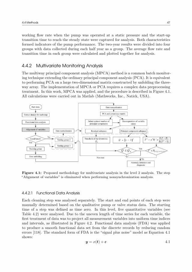
4.4 Methods 47
working flow rate when the pump was operated at a static pressure and the start-uptransition time to reach the steady state were captured for analysis. Both characteristicsformed indicators of the pump performance. The two-year results were divided into fourgroups with data collected during each half year as a group. The average flow rate andtransition time in each group were calculated and plotted together for analysis.
4.4.2 Multivariate Monitoring AnalysisThe multiway principal component analysis (MPCA) method is a common batch monitor-ing technique extending the ordinary principal component analysis (PCA). It is equivalentto performing PCA on a large two-dimensional matrix constructed by unfolding the three-way array. The implementation of MPCA or PCA requires a complex data preprocessingtreatment. In this work, MPCA was applied, and the procedure is described in Figure 4.1.All calculations were carried out in Matlab (Mathworks, Inc., Natick, USA).
Figure 4.1: Proposed methodology for multivariate analysis in the level 2 analysis. The step“Alignment of variables” is eliminated when performing nonsynchronization analysis.
4.4.2.1 Functional Data Analysis
Each cleaning step was analysed separately. The start and end points of each step weremanually determined based on the qualitative pump or valve status data. The startingtime of a step was defined as time zero. In this level, five quantitative variables (seeTable 4.2) were analysed. Due to the uneven length of time series for each variable, thefirst treatment of data was to project all measurement variables into uniform time indicesand intervals, as illustrated in Figure 4.2. Functional data analysis (FDA) was appliedto produce a smooth functional data set from the discrete records by reducing randomerrors [118]. The standard form of FDA is the “signal plus noise” model as Equation 4.1shows:
y = x(t) + ε 4.1
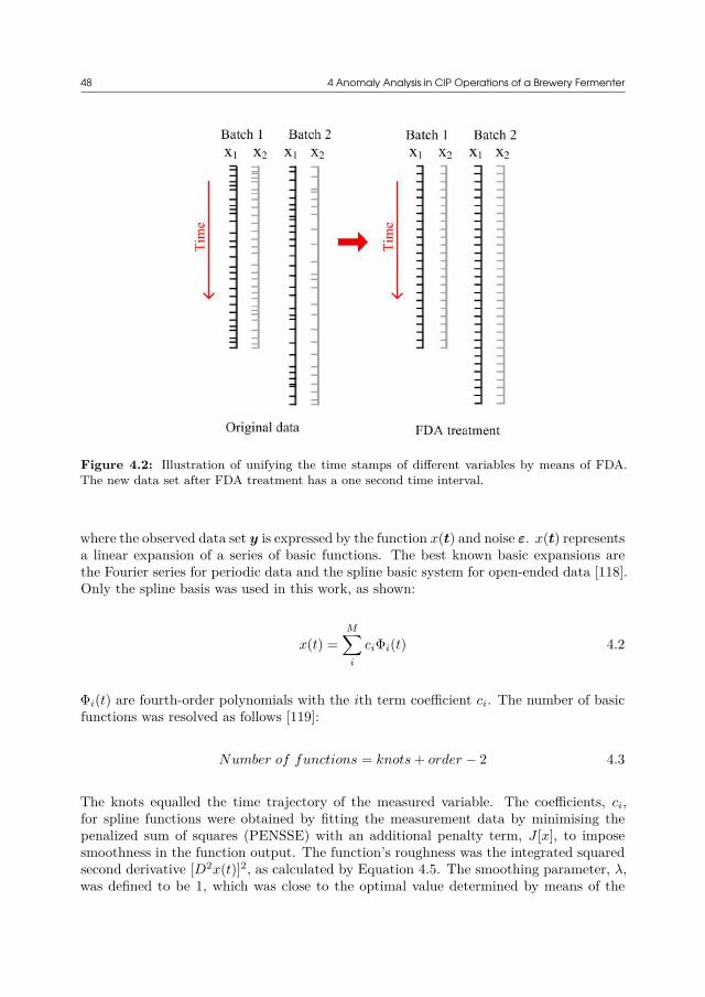
48 4 Anomaly Analysis in CIP Operations of a Brewery Fermenter
Figure 4.2: Illustration of unifying the time stamps of different variables by means of FDA.The new data set after FDA treatment has a one second time interval.
where the observed data set y is expressed by the function x(t) and noise ε. x(t) representsa linear expansion of a series of basic functions. The best known basic expansions arethe Fourier series for periodic data and the spline basic system for open-ended data [118].Only the spline basis was used in this work, as shown:
x(t) =M∑i
ciΦi(t) 4.2
Φi(t) are fourth-order polynomials with the ith term coefficient ci. The number of basicfunctions was resolved as follows [119]:
Number of functions = knots + order − 2 4.3
The knots equalled the time trajectory of the measured variable. The coefficients, ci,for spline functions were obtained by fitting the measurement data by minimising thepenalized sum of squares (PENSSE) with an additional penalty term, J [x], to imposesmoothness in the function output. The function’s roughness was the integrated squaredsecond derivative [D2x(t)]2, as calculated by Equation 4.5. The smoothing parameter, λ,was defined to be 1, which was close to the optimal value determined by means of the
4.4 Methods 49
generalized cross-validation (GCV) criterion [118, 119].
PENSSE =n∑i
(yi − x(ti))2 + λ × J [x] 4.4
J [x] =∫
[D2x(t)]2dt 4.5
In order to unify the time trajectories for all variables, a new time vector with one secondinterval was defined. The values of different variables in the new time series were evaluatedfrom the smoothed functions.
4.4.2.2 Alignment of Variable Trajectories
FDA aligns different variables within a batch. However, following FDA, the unequal andunaligned data across batches still exist because the original data were collected withindependent lengths. Three approaches were tested to solve the problem:
1. The first and the simplest method was to cut all batches to the minimum length or aspecific length. This method kept the nature of batches, at the expense of losing allinformation after the cutting point. However, the shifts of variable profiles causedby the dynamic operation of the pump could still lead to the challenges of dataanalysis.
2. The second method was the indicator variable technique, the concept of which wasto replace time by another process or derived variable to indicate the progress ofa batch [120]. In this study, the liquid volumetric consumption, calculated fromtime and flow rate data, was chosen as the indicator variable to quantify the per-cent completion of cleaning. Linear interpolation was used to transform the timedimension into the indicator variable dimension.
3. The third method was to locally translate, compress, and expand the pattern ofone sequence to match another sequence of similar features, called dynamic timewarping (DTW) [121]. DTW non-linearly warps two data series in such a way thatsimilar events are aligned and the distance between them is minimized [117]. In thisstudy, pressure was an active variable, whose variance influenced the patterns ofother variables. Therefore, the warping path was obtained by aligning all pressuremeasurements to a reference batch demonstrating good performance, and othervariables within a batch were aligned in the same warping path.
4.4.2.3 Training and Testing Data Sets
The CIP batches were labeled as “good” or “bad” operations. A CIP batch was regardedas bad when possessing at least one of the following characteristics:
• the pump stopped for an uncommonly long time during a step;
• there were more or less pump stops than foreseen in a normal operation procedure;
50 4 Anomaly Analysis in CIP Operations of a Brewery Fermenter
• a cleaning step was missing, or the duration of a step was extremely long or short;
• the ionic properties of chemical solutions were abnormal;
• unreasonable flow rates were observed (i.e., zero flow rate due to pump idling).
Ca. 15 good batches, the number of which varied when analysing different cleaning steps,were used as training data set for constructing the reference models. The rest, consistingof both good and bad batches, were used as testing data set for validating the models.
4.4.2.4 Data Unfolding and Normalization
The functional data were provided as a three-dimensional (3D) matrix with I batches,J time indices, and K variables. MPCA requires that the 3D matrix is unfolded to atwo-dimensional (2D) matrix. There are normally two ways to unfold batch data: abatch-wise unfolding results in an (I × JK) matrix and a variable-wise unfolding yieldsan (IJ × K) matrix. Most statistical process monitoring techniques apply the batch-wise unfolding approach, allowing one to analyse the variability among batches withrespect to variables and their time variation. However, when being used online, it isrequired to estimate the future portions of variable trajectories. On the contrary, thevariable-wise unfolding does not require such estimation, making it applicable for onlinemonitoring [115, 122, 123]. Wold et al. (1998) concluded that the former was oriented toevaluating the completed batch as normal or abnormal, while the latter focused more onthe monitoring of individual time points [124]. The primary objective of this study wasto identify the occurrence of an anomalous event online. Therefore, only the variable-wiseunfolding method was applied to the data.
The new unfolded matrix was then mean-centered and variance scaled. Mean centeringwas applied to the raw data by subtracting the average variable values for each time point.Then the variance scaling was carried out to the centered data by a slab-scaling method,by dividing with a unit root-mean-square of each variable. We noted that other scalingmethods, like column-scaling by dividing the root-mean-square of each time point, led todifferent results. In pre-studies, lower variability was explained when scaling with column-scaling, because this method caused significant deviations when data were unsynchronizedor inadequately synchronized. Therefore, only the robust slab-scaling method was used inthis study, which was also recommended when dealing with an industrial data set [125].
4.4.2.5 Multivariate Analysis
PCA is a commonly used multivariate statistical analysis method for monitoring purposes,which defines the principal components through a linear transformation of the originalvariables and explains the maximum variance. Instead of analysing all variables, the PCAmethod focuses only on analysing the principal components when monitoring the systemand thereby reduces the dimensionality of data [122, 124]. In this work, PCA was appliedto the normalized data matrix X, which was decomposed into a score matrix T and aprincipal loading matrix P :
X = TP T 4.6
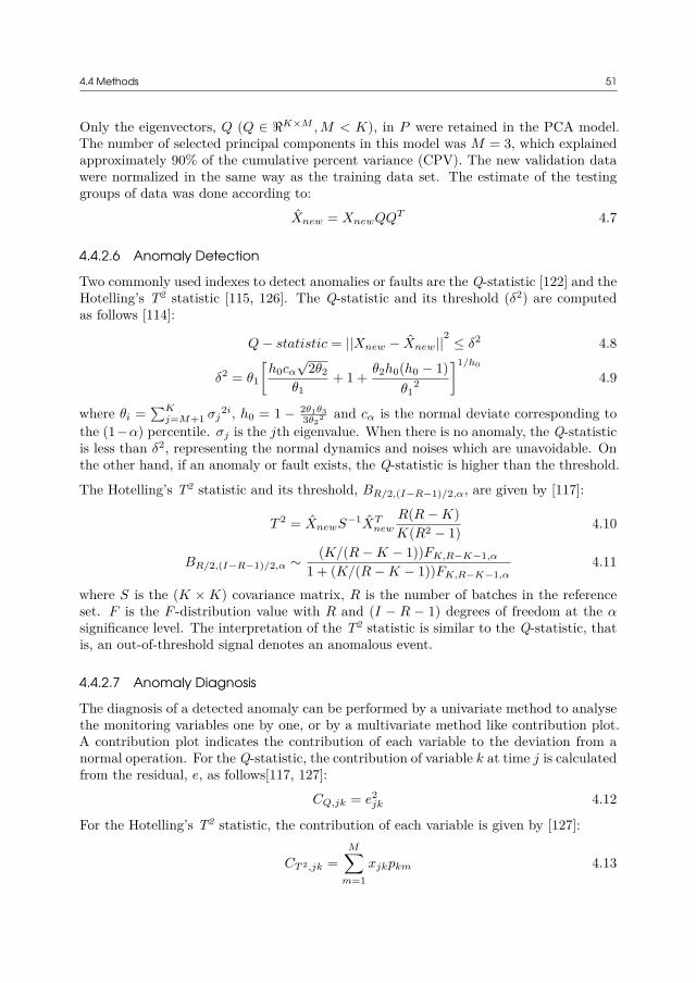
4.4 Methods 51
Only the eigenvectors, Q (Q ∈ ℜK×M , M < K), in P were retained in the PCA model.The number of selected principal components in this model was M = 3, which explainedapproximately 90% of the cumulative percent variance (CPV). The new validation datawere normalized in the same way as the training data set. The estimate of the testinggroups of data was done according to:
Xnew = XnewQQT 4.7
4.4.2.6 Anomaly Detection
Two commonly used indexes to detect anomalies or faults are the Q-statistic [122] and theHotelling’s T2 statistic [115, 126]. The Q-statistic and its threshold (δ2) are computedas follows [114]:
Q − statistic = ||Xnew − Xnew||2
≤ δ2 4.8
δ2 = θ1
[h0cα
√2θ2
θ1+ 1 + θ2h0(h0 − 1)
θ12
]1/h0
4.9
where θi =∑K
j=M+1 σj2i, h0 = 1 − 2θ1θ3
3θ22 and cα is the normal deviate corresponding tothe (1−α) percentile. σj is the jth eigenvalue. When there is no anomaly, the Q-statisticis less than δ2, representing the normal dynamics and noises which are unavoidable. Onthe other hand, if an anomaly or fault exists, the Q-statistic is higher than the threshold.
The Hotelling’s T2 statistic and its threshold, BR/2,(I−R−1)/2,α, are given by [117]:
T 2 = XnewS−1XTnew
R(R − K)K(R2 − 1)
4.10
BR/2,(I−R−1)/2,α ∼ (K/(R − K − 1))FK,R−K−1,α
1 + (K/(R − K − 1))FK,R−K−1,α4.11
where S is the (K × K) covariance matrix, R is the number of batches in the referenceset. F is the F -distribution value with R and (I − R − 1) degrees of freedom at the αsignificance level. The interpretation of the T2 statistic is similar to the Q-statistic, thatis, an out-of-threshold signal denotes an anomalous event.
4.4.2.7 Anomaly Diagnosis
The diagnosis of a detected anomaly can be performed by a univariate method to analysethe monitoring variables one by one, or by a multivariate method like contribution plot.A contribution plot indicates the contribution of each variable to the deviation from anormal operation. For the Q-statistic, the contribution of variable k at time j is calculatedfrom the residual, e, as follows[117, 127]:
CQ,jk = e2jk 4.12
For the Hotelling’s T2 statistic, the contribution of each variable is given by [127]:
CT 2,jk =M∑
m=1xjkpkm 4.13

52 4 Anomaly Analysis in CIP Operations of a Brewery Fermenter
where pkm is the loading for variable k in dimension m.
4.4.3 End-of-Batch Performance EvaluationFor level 3 of the approach, a standard range was defined for the cleaning time, liquidconsumption or on−off ratio (the period when the pump is “on” divided by the wholestep time) of each step on the basis of some good batches. The standard was made foreach cleaning step, including the means, standard deviations (STD), and a parameter γ,to allow a judgement range as described in Equation 4.14.
Reference = mean ± γ × STD 4.14
The testing groups of data were used for validation, which included both good and badbatches (defined in section 4.4.2.3). During the test, a cleaning was regarded as “normal”if the indexes were within the reference range. On the contrary, a cleaning was “abnormal”if the indexes were out of the range. However, wrong judgement might occur. For example,a good operation was denoted as bad or a bad operation was denoted as good. Therefore,there are four possible outcomes [128]: (1) true positive (TP) correctly recognizes a goodoperation as “good”; (2) true negative (TN) correctly recognizes a bad operation as“bad”; (3) false positive (FP) wrongly recognizes a bad operation as “good”; and (4) falsenegative (FN) wrongly recognizes a good operation as “bad”.
The judgement decision depends on the value of γ. Therefore, a new index, η, was definedto quantify the ratio of the number of correct judgements over the total number of testingbatches, as present in Equation 4.15. A high value of η represents a high probability tomake a right decision.
η = 1 − FP + FN
All4.15
4.5 Results and Discussion
4.5.1 Precleaning: Performance of the Feed PumpFigure 4.3 displays the performance of the feed pump over a two-year period. The start-up transition time for the feed pump to reach the working flow rate has not changedsignificantly (p = 0.23), but the static flow rate reveals a clearly decreasing trend (p <0.01). The decrease of flow rate may result in insufficient mechanical force to remove soilsfrom the surface, or make the cleaning costs extremely high. This decreasing trend offlow rate can be due to the mechanical variance of the pump, leaking of liquid, fouling ofthe transfer pipe, low level of liquid in the storage tank, calibration of sensors, etc. Sincethe variance of flow rate is a long-term performance metric, the occasional faults can beignored, like the leaking problem and the liquid level. However, it is still difficult to findan exact cause of the anomaly due to the lack of measurement.
The differential pressure (the difference between the suction and discharge heads) is crit-ical for a pressure-controlled pump, as in this case. For example, the outlet pressure iscontrolled to be constant. However, if there is fouling in the suction line, the inlet pressure

4.5 Results and Discussion 53
Figure 4.3: Working flow rate and start-up transition time of the feed pump over the past twoyears.
drops and the differential pressure increases, and consequently the flow rate drops. Onthe other hand, the fouling in the discharging line (which is to be cleaned) can increasethe system friction and reduce the flow rate as well [129]. Besides, the cavitation of thepump and the change of impeller clearance can influence the pump performance. As aresult, the observation in Figure 4.3 reminds the operators to perform an inspection ofthe pump or of the whole system. There is a risk of failure once the flow rate is less thanthe critical point.
The above-mentioned analysis can be accomplished automatically if the system can ex-tract the flow rate information based on previous cleaning operations by coupling thepump status and output, thereby displaying the performance of the feed pump before anew operation starts. A similar analysis can be applied to other systems besides the feedpump. For example, checking heat exchangers’ working temperature and heating timeto reach the critical temperature can characterize the performance of heat exchangers(though irrelevant in this study). Keeping the whole system in high performance is aprerequisite to avoid a potential cleaning failure.
4.5.2 Cleaning or Post Cleaning: Data Pretreatment and MPCAModel
The multivariate analysis was performed for each step separately. An example of the FDAresults for the alkaline treatment without circulation step is shown in Figure 4.4. Thesmoothness is controlled by the penalty coefficient, λ, in Equation 4.4. For the alkalinestep, the optimal λ determined by the GCV criterion varies from batch to batch andvariable to variable, most of which lie in the range of 10-1 ∼ 101. Choosing a small value
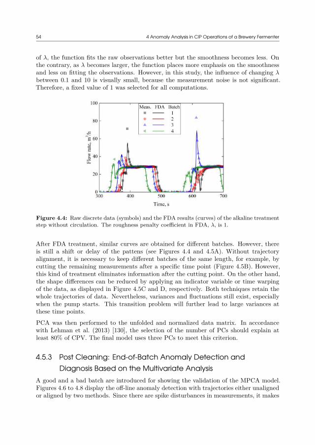
54 4 Anomaly Analysis in CIP Operations of a Brewery Fermenter
of λ, the function fits the raw observations better but the smoothness becomes less. Onthe contrary, as λ becomes larger, the function places more emphasis on the smoothnessand less on fitting the observations. However, in this study, the influence of changing λbetween 0.1 and 10 is visually small, because the measurement noise is not significant.Therefore, a fixed value of 1 was selected for all computations.
Figure 4.4: Raw discrete data (symbols) and the FDA results (curves) of the alkaline treatmentstep without circulation. The roughness penalty coefficient in FDA, λ, is 1.
After FDA treatment, similar curves are obtained for different batches. However, thereis still a shift or delay of the pattens (see Figures 4.4 and 4.5A). Without trajectoryalignment, it is necessary to keep different batches of the same length, for example, bycutting the remaining measurements after a specific time point (Figure 4.5B). However,this kind of treatment eliminates information after the cutting point. On the other hand,the shape differences can be reduced by applying an indicator variable or time warpingof the data, as displayed in Figure 4.5C and D, respectively. Both techniques retain thewhole trajectories of data. Nevertheless, variances and fluctuations still exist, especiallywhen the pump starts. This transition problem will further lead to large variances atthese time points.
PCA was then performed to the unfolded and normalized data matrix. In accordancewith Lehman et al. (2013) [130], the selection of the number of PCs should explain atleast 80% of CPV. The final model uses three PCs to meet this criterion.
4.5.3 Post Cleaning: End-of-Batch Anomaly Detection andDiagnosis Based on the Multivariate Analysis
A good and a bad batch are introduced for showing the validation of the MPCA model.Figures 4.6 to 4.8 display the off-line anomaly detection with trajectories either unalignedor aligned by two methods. Since there are spike disturbances in measurements, it makes
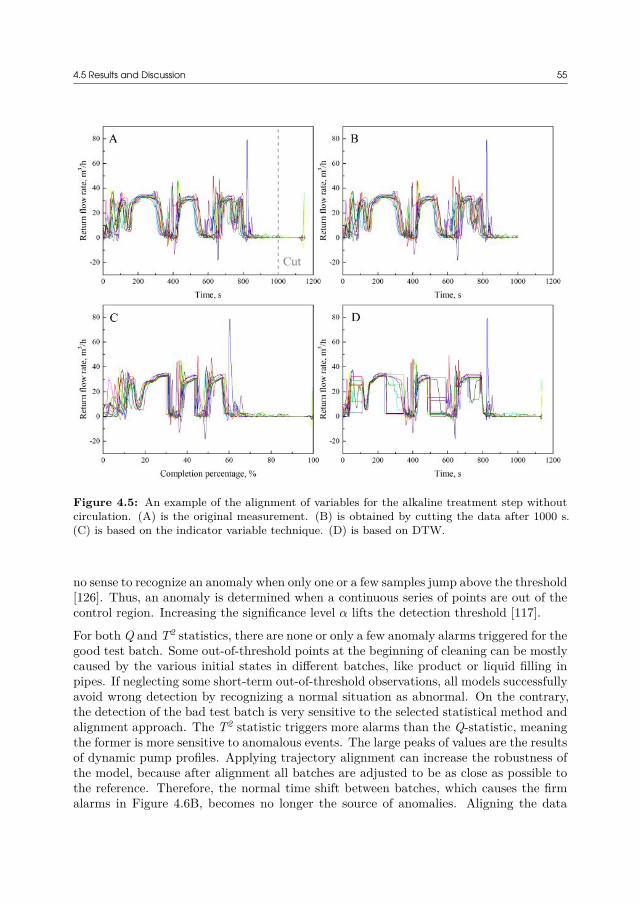
4.5 Results and Discussion 55
Figure 4.5: An example of the alignment of variables for the alkaline treatment step withoutcirculation. (A) is the original measurement. (B) is obtained by cutting the data after 1000 s.(C) is based on the indicator variable technique. (D) is based on DTW.
no sense to recognize an anomaly when only one or a few samples jump above the threshold[126]. Thus, an anomaly is determined when a continuous series of points are out of thecontrol region. Increasing the significance level α lifts the detection threshold [117].
For both Q and T2 statistics, there are none or only a few anomaly alarms triggered for thegood test batch. Some out-of-threshold points at the beginning of cleaning can be mostlycaused by the various initial states in different batches, like product or liquid filling inpipes. If neglecting some short-term out-of-threshold observations, all models successfullyavoid wrong detection by recognizing a normal situation as abnormal. On the contrary,the detection of the bad test batch is very sensitive to the selected statistical method andalignment approach. The T2 statistic triggers more alarms than the Q-statistic, meaningthe former is more sensitive to anomalous events. The large peaks of values are the resultsof dynamic pump profiles. Applying trajectory alignment can increase the robustness ofthe model, because after alignment all batches are adjusted to be as close as possible tothe reference. Therefore, the normal time shift between batches, which causes the firmalarms in Figure 4.6B, becomes no longer the source of anomalies. Aligning the data
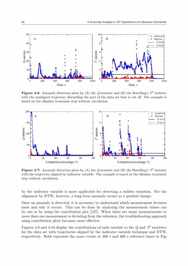
56 4 Anomaly Analysis in CIP Operations of a Brewery Fermenter
Figure 4.6: Anomaly detection plots by (A) the Q-statistic and (B) the Hotelling’s T2 statisticwith the unaligned trajectory discarding the part of the data set that is cut off. The example isbased on the alkaline treatment step without circulation.
Figure 4.7: Anomaly detection plots by (A) the Q-statistic and (B) the Hotelling’s T2 statisticwith the trajectory aligned by indicator variable. The example is based on the alkaline treatmentstep without circulation.
by the indicator variable is more applicable for detecting a sudden variation. For thealignment by DTW, however, a long-term anomaly occurs as a gradual change.
Once an anomaly is detected, it is necessary to understand which measurement deviatesmost and why it occurs. This can be done by analysing the measurement values oneby one or by using the contribution plot [127]. When there are many measurements ormore than one measurement is deviating from the reference, the troubleshooting approachusing contribution plots becomes more effective.
Figures 4.9 and 4.10 display the contributions of each variable to the Q and T2 statisticsfor the data set with trajectories aligned by the indicator variable technique and DTW,respectively. Both represent the same events at 300 s and 400 s reference times in Fig-
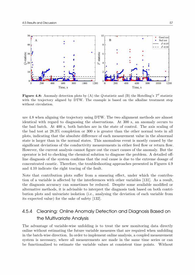
4.5 Results and Discussion 57
Figure 4.8: Anomaly detection plots by (A) the Q-statistic and (B) the Hotelling’s T2 statisticwith the trajectory aligned by DTW. The example is based on the alkaline treatment stepwithout circulation.
ure 4.8 when aligning the trajectory using DTW. The two alignment methods are almostidentical with regard to diagnosing the observations. At 300 s, an anomaly occurs tothe bad batch. At 400 s, both batches are in the state of control. The axis scaling ofthe bad test at 28.3% completion or 300 s is greater than the other normal tests in allplots, indicating that the absolute difference of each measurement value in the abnormalstate is larger than in the normal states. This anomalous event is mostly caused by thesignificant deviations of the conductivity measurements in either feed flow or return flow.However, the current analysis cannot figure out the exact causes of the anomaly. But theoperator is led to checking the chemical solution to diagnose the problem. A detailed off-line diagnosis of the system confirms that the real cause is due to the extreme dosage ofconcentrated caustic. Therefore, the troubleshooting approaches presented in Figures 4.9and 4.10 indicate the right tracing of the fault.
Note that contribution plots suffer from a smearing effect, under which the contribu-tion of a variable is affected by the interferences with other variables [131]. As a result,the diagnosis accuracy can sometimes be reduced. Despite some available modified oralternative methods, it is advisable to interpret the diagnosis task based on both contri-bution plots and univariate isolation (i.e., analysing the deviation of each variable fromits expected value) for the sake of safety [132].
4.5.4 Cleaning: Online Anomaly Detection and Diagnosis Based onthe Multivariate Analysis
The advantage of variable-wise unfolding is to treat the new monitoring data directlyonline without estimating the future variable measures that are required when unfoldingin the batch-wise direction. In order to implement online analysis, a coupled measurementsystem is necessary, where all measurements are made in the same time series or canbe functionalized to estimate the variable values at consistent time points. Without
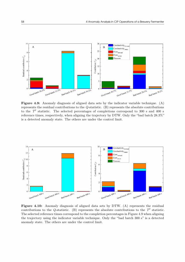
58 4 Anomaly Analysis in CIP Operations of a Brewery Fermenter
Figure 4.9: Anomaly diagnosis of aligned data sets by the indicator variable technique. (A)represents the residual contributions to the Q-statistic. (B) represents the absolute contributionsto the T2 statistic. The selected percentages of completions correspond to 300 s and 400 sreference times, respectively, when aligning the trajectory by DTW. Only the “bad batch 28.3%”is a detected anomaly state. The others are under the control limit.
Figure 4.10: Anomaly diagnosis of aligned data sets by DTW. (A) represents the residualcontributions to the Q-statistic. (B) represents the absolute contributions to the T2 statistic.The selected reference times correspond to the completion percentages in Figure 4.9 when aligningthe trajectory using the indicator variable technique. Only the “bad batch 300 s” is a detectedanomaly state. The others are under the control limit.
4.5 Results and Discussion 59
trajectory alignment, the new monitoring variables can be directly unfolded, normalized,PCA transformed, and analysed by statistics as illustrated in Figure 4.1. Similar resultscan be obtained as shown in Figure 4.6. However, the unaligned approach results inhigh uncertainty once normal time shifting is significant in the new batch. In this regard,trajectory alignment becomes more credible, plus more challenging.
For the alignment according to an indicator variable, the completion percentage is calcu-lated from the consumption of liquid volume divided by the total consumption. However,the actual total consumption of liquid is unknown until the end of the batch. Therefore, aconstant value of the average consumption in reference batches is used for the new batch.This value can be altered to the real consumption when performing an end-of-batch anal-ysis.
For the alignment using DTW, the challenge in online monitoring is to pair the currentobservation time to an end point in the reference in order to synchronize the new trajectorywith the reference timeline. Kassidas et al. (1998) introduced lower and upper bounds forsearching the optimal path that provides the best matching between the reference andthe uncompleted batch [133]. The point resulting in the minimal accumulated distanceis determined as the end point corresponding to the current observation. In the study ofthis chapter, the alignment path can be obtained by aligning the pressure intensity alongthe reference timeline. This procedure is one-way incremental and repeated when eachnew measurement comes in.
To explain online monitoring, an example is shown in Figure 4.11 based on functionalizeddata. In Figure 4.11A, the difference between the online and offline aligned data is due tothe fact that the real overall consumption may differ from the expected value. However,the deviation only causes a slight shift of the profile. The alignment based on DTW canalso effectively reduce the time difference (see Figure 4.11B). However, caution should betaken when defining the searching bounds of the end point, which should lie internallybetween the lower and upper bounds. To sum up, the indicator variable based approachsurpasses the DTW method in terms of computation efficiency because the latter requiresaccumulative calculations of all likely points in the range in order to obtain the minimaldistance. After alignment, the new monitoring variables can be further transformed foranomaly detection, as described in Figure 4.1.
4.5.5 Post Cleaning: Validation of PerformanceOperators expect a simple method to evaluate a CIP operation, by indicators which canbe easily measured or computed, such as the step time, the liquid consumption, and theon−off ratio of the pump. Therefore, the operators only need to compare these values withthe standard ranges and get an idea about whether the cleaning is performed accordingly.The standard range is related to the safety margin parameter, λ, which further influencesthe judgement of the cleaning performance.
As shown in Figure 4.12, the increase in λ generally improves the correctness of thejudgement, as more good cleaning operations are covered in the range. However, if thevalue of λ is beyond a specific limit, the correctness of the judgement is reduced, because
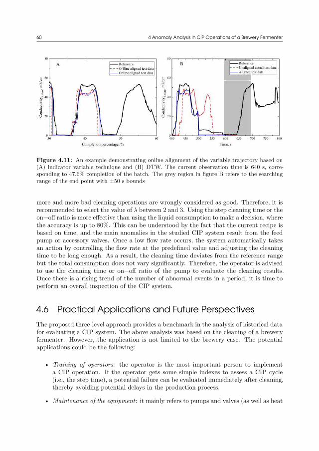
60 4 Anomaly Analysis in CIP Operations of a Brewery Fermenter
Figure 4.11: An example demonstrating online alignment of the variable trajectory based on(A) indicator variable technique and (B) DTW. The current observation time is 640 s, corre-sponding to 47.6% completion of the batch. The grey region in figure B refers to the searchingrange of the end point with ±50 s bounds
more and more bad cleaning operations are wrongly considered as good. Therefore, it isrecommended to select the value of λ between 2 and 3. Using the step cleaning time or theon−off ratio is more effective than using the liquid consumption to make a decision, wherethe accuracy is up to 80%. This can be understood by the fact that the current recipe isbased on time, and the main anomalies in the studied CIP system result from the feedpump or accessory valves. Once a low flow rate occurs, the system automatically takesan action by controlling the flow rate at the predefined value and adjusting the cleaningtime to be long enough. As a result, the cleaning time deviates from the reference rangebut the total consumption does not vary significantly. Therefore, the operator is advisedto use the cleaning time or on−off ratio of the pump to evaluate the cleaning results.Once there is a rising trend of the number of abnormal events in a period, it is time toperform an overall inspection of the CIP system.
4.6 Practical Applications and Future PerspectivesThe proposed three-level approach provides a benchmark in the analysis of historical datafor evaluating a CIP system. The above analysis was based on the cleaning of a breweryfermenter. However, the application is not limited to the brewery case. The potentialapplications could be the following:
• Training of operators: the operator is the most important person to implementa CIP operation. If the operator gets some simple indexes to assess a CIP cycle(i.e., the step time), a potential failure can be evaluated immediately after cleaning,thereby avoiding potential delays in the production process.
• Maintenance of the equipment: it mainly refers to pumps and valves (as well as heat

4.6 Practical Applications and Future Perspectives 61
Figure 4.12: Ratio of the correct judgement of cleaning performance against the margin pa-rameter λ: (A) alkaline step without circulation, (B) alkaline circulation, (C) acid circulation,and (D) disinfectant circulation. There are no pump stops during the alkaline circulation step.
exchangers, though not involved in this chapter). A systematic shift of observations(i.e., flow rate and transition time) may indicate an accumulated error or damageof the equipment.
• Optimization of the system: a reference model has been established based on his-torical data of good cleaning operations. Optimization could therefore be achievedby altering one parameter once and comparing the new measurements with thereference.
• Flexible selection of cleaning recipes: in some processes where the equipment is usedto produce different products, there are multiple recipes to remove different soilingmaterials when altering products. A reference model helps to examine if a complexrecipe is selected to clean a loose soil or a simple recipe is selected to clean a harshsoil. Sometimes, a short cleaning recipe should be selected before production if theequipment is held for a long time. Choosing a full recipe in this case will wasteconsiderable money and resources. A reference model helps to recognise the recipe,because an improper selection of recipe results in unexpected monitoring outputswhen comparing with the reference.
62 4 Anomaly Analysis in CIP Operations of a Brewery Fermenter
• Alarm of system anomaly: conventionally, the alarm is triggered when one or moremonitoring variables are out of range, meaning that the failure or error alreadyhappens. A multivariate analysis approach can not only capture such an existingproblem but also identify abnormal trends that may suggest a potential failure.Early detection of anomalies reduces the damage of equipment and saves cleaningresources.
• Counting of anomalous events: end-of-batch analysis can be performed periodicallyby counting anomalies over a specific period, in order to gain a better understandingof the system.
There are some considerations associated with the existing study to support an effectiveapplication in the future. First, only the two-year data set of one brewery fermenter isinvestigated. As a benchmark case, the model is flexible to involve other systems andmore data sets. Second, the current system does not consist of any online monitoringof cleaning quality, which is a common problem in most CIP practices. New sensortechnology (i.e., turbidity) allows to detect the residues in the liquid phase. Involving thequality indicators of the cleaning operation into the second level analysis will deliver moreinformation and potentially allow to predict the end point of cleaning operations [115].Finally, an advanced monitoring and control system is required to implement the analysisautomatically. Especially, monitoring all variables of the same trajectory and equal timespace should allow simplifying the model construction and reducing the uncertainty. Anideal operation of CIP is expected to be implemented in such a manner:
1. when clicking the recipe button, the control interface displays the system perfor-mance based on previous cleaning operations and offline measurements, and reportsif the selected recipe is able to complete the cleaning task in an efficient and eco-nomic manner;
2. when performing the cleaning, the abnormal detection approach triggers the alarmimmediately when it happens, and the potential causes of anomalies and proposedactions are described;
3. after cleaning, a report is automatically generated including the cleaning duration,the chemical consumption, and the number of anomalies, as well as a self-evaluationof the result.
4.7 ConclusionsA three-level analysis approach was described to provide a benchmark to analyse historicaldata in CIP cycles. The case study analysed here was based on the cleaning of a fermenterin an industrial brewery. Reference models were established in order to evaluate if thefuture cleaning operations are performed normally or abnormally. The analysis approachis expected to be carried out prior to cleaning, during cleaning and at the end of thecleaning process.
4.7 Conclusions 63
In the demonstrated case of the cleaning of a brewery fermenter, a decreasing trend ofthe feed pump performance is observed, indicating the necessity of an overall inspectionof the system. The process monitoring using multivariate analysis methods is able todetect the localized abnormal events in the process. Trajectory alignment is necessary toovercome time shifting between batches and hence improve the robustness of the model.Using the liquid volume consumption as an indicator variable to synchronize the dataset is more efficient than DTW in terms of computation speed. Both Q-statistic andHotelling’s T2 statistic can indicate the occurrence of an anomalous event. Contributionplots can help to diagnose the cause of an anomaly. When the cleaning is finished, theoperators are advised to check the cleaning time or on−off ratio of the pump to evaluateif the cleaning has been performed consistently.
The application of the proposed analysis approach is not limited to the CIP operationsof the brewery fermenter. The possible applications are to utilize historical knowledgeto benefit the daily operations, the maintenance and optimization of the system, andthe monitoring of new cycles, in order to gain a deeper understanding of the processand reduce cleaning costs. The model is flexible to involve more data to make it moreinformative. An ideal situation is to automatically detect and diagnose the anomalies inthe system with the help of advanced monitoring and control systems.
List of Nomenclature in Chapter 4The following nomenclature is only valid for this chapter. Some symbols are used in otherchapters but with different meanings. Otherwise, the symbols are specifically explainedin the text if there is no nomenclature in some chapter.
Roman LettersB The threshold of Hotelling’s T2 statisticc The coefficient of the basic functioncα The normal deviation corresponding to the (1 − α) percentileCQ Contribution to the Q-statisticCT 2 Contribution to the Hotelling’s T2 statistice ResidualF The F -distribution valueh0 A coefficient for computing the threshold of the Q-statisticI Number of batchesJ Number of time indicesJ [x] Roughness termK Number of variablesM Number of principal componentsp Probability valuepkm Loading for variable k in dimension mP Loading matrixQ Principal loading matrixR Number of batches in the reference setS Covariance matrix
64 4 Anomaly Analysis in CIP Operations of a Brewery Fermenter
t Time, [s]T PCA scoresT 2 Hotelling’s T2 statisticx The predicted function in FDAX The matrix of variablesy The observed data set in FDA
Greek Lettersα Significance levelσj The jth eigenvalueε The noise term in FDAΦ Basic functionγ Safety marginη The ratio of correct judgementλ Roughness penalty coefficientδ2 The threshold of the Q-statisticθi the ith coefficient for computing the threshold of the Q-statistic
CHAPTER5Simulations of BlendingPhases in Pipe Systems
Using CFDIn this chapter, CFD is used to simulate the blending phase problems in the rinsingof different pipe elements. The work was performed in collaboration with Alfa LavalCopenhagen A/S and Carlsberg Danmark A/S. Part of this chapter about the simulationof straight pipes has been published and reproduced based on the following article [134]:
CFD modelling of axial mixing in the intermediate and final rinses of cleaning-in-placeprocedures of straight pipesYang, J., Jensen, B. B. B., Nordkvist, M., Rasmussen, P., Gernaey, K. V., Krühne, U.Journal of Food Engineering, 221: 95 - 105. (2018)DOI: 10.1016/j.jfoodeng.2017.09.017
5.1 Introduction
5.1.1 Blending Phase ProblemsChapter 3 has presented that in the cleaning of pipes and tanks at the mapped brewery,nearly 60% of the cleaning costs attribute to the pipe cleaning operations. Most of thecleaning time and costs are spent on the alkaline/acid treatment, disinfection and threerinsing steps (two intermediate rinses and one final rinse). The recovery of the cleaningdetergents can be up to 95% of the supply. In some industries, the final rinsing watercan be partly recycled for the pre-rinse of the next CIP. The intermediate rinsing wateris rarely recycled. Therefore, the overall recovery efficiency of rinsing water is very low,even less than 10%. Most of the rinsing water is directly disposed to drain.
Cleaning generates large amounts of waste water containing corrosive pollutants, nutri-ents, and potentially a considerable organic load. Furthermore, heat losses due to thedischarge of hot water contribute significantly to the overall costs. Minimizing the con-sumption of resources (water, chemical and electrical energy, etc.) is of great importance
66 5 Simulations of Blending Phases in Pipe Systems Using CFD
due to strict legislative and environmental regulations [135]. A number of studies havefocused on the development of new cleaning agents, the effect of water quality and theoptimization of chemical usage [1, 93, 136]. However, industrial applications of suchtechnologies are still limited due to the complex alteration of existing equipment and theinestimable payback time. Operators prefer simple changes in operations without signif-icant transformation of the existing processes. Therefore, reducing water consumptionby optimizing the flow rate and rinsing time in rinsing steps and improving the recoveryefficiency of cleaning agents becomes a practical solution for many food industries, as theoperators can easily change and dynamically adapt these parameters at the control panel.
The objective of rinsing is to displace the residual cleaning agents (alkaline, acid anddisinfectant) and reduce cross-contamination risks [6]. Such displacement of one liquid(chemical agent) with another liquid (water) occurs at the blending phase of the twoliquids, where an axial mixing zone is created due to convection and diffusion phenomena[137]. The knowledge about axial mixing and displacement is of importance in order toensure complete chemical removal at reduced water consumption.
5.1.2 CFD and Numerical ModelsSection 2.6.2 has provided some applications of CFD in understanding and predicting fluidflow by predicting the wall shear stress (WSS) on surfaces. Nearly all of these CFD studiesapplied to CIP consider water as the medium to remove soils from the surfaces. Thereare, to our knowledge, no CFD investigations by other researchers about the intermediateor final rinses where water is mainly used to displace the cleaning agents. Compared withanalytical mathematical models, the use of CFD models can get the information aboutmixing in both axial and radial directions. In some cases, CFD models can replace on-linemeasurements, as the installation of probes increases the capital costs and may introducenew areas that are difficult to clean. Moreover, CFD applies to complex geometries andis very helpful for the hygienic design of a pipe system.
In CFD simulations, the Navier-Stokes equation for incompressible flow reads:
ρ(∂ui
∂t+ uj
∂ui
∂xj
)= − p
∂xi+ ∂
∂xj
(µ
∂ui
∂xj
)5.1
where ρ is the fluid density and µ is the dynamic viscosity. u, x and t are velocity,coordinate and time, respectively. The time-dependent convection-diffusion equation fora scalar transport with concentration C is as follows:
∂C
∂t+ ui
∂C
∂xi= ∂
∂xi
(D
∂C
∂xi
)5.2
where D is the dispersion coefficient. In the case of turbulent flow, the dispersion consistsprincipally of two contributions, caused by molecular diffusion and turbulent eddies. Inliquid mixtures, the concentration diffusion flux J in the ith coordinate can be describedas follows:
Ji = −(
D0 + νt
Sct
) ∂C
∂xi5.3
5.2 Methods 67
where D0 is the molecular diffusion coefficient; Sct is the turbulent Schmidt numbercalculated by the turbulent kinetic viscosity νt and the turbulent diffusivity Dt throughSct = νt/Dt. Mathematically, dispersion can be treated in the same manner as moleculardiffusion [138]. In a turbulent regime, the contribution of molecular diffusion is much lessthan that of turbulent eddies.
5.1.3 Objective of This ChapterPipe systems include various types of elements, e.g., straight pipes, bends, T-joints, ex-pansions, contractions and valves (mixing valves, butterfly valves, ball valves, air-blowvalves, etc.). The cleaning difficulties vary depending on the design of these elementsand the operating conditions. Investigating single and simple geometries is an importantstep if a complex geometry with various pipe elements is going to be studied. Therefore,the purpose of this chapter is to simulate the blending phase problems, including axialmixing and the displacement phenomenon, in the intermediate and final rinses of CIPprocedures for different pipe elements using CFD.
A detailed understanding of the blending phase problems in CIP supports the knowledgeabout the effects of flow patterns on the process. The minimal time required to completelydisplace the residual agents can be predicted. Furthermore, the total water consumptioncan be minimized by a proper combination of flow rate and rinsing time as well as by theimplementation of efficient recovery plans.
This chapter describes two steps. The first step is to simulate the simplest straightpipe geometries. The results are validated using published empirical results based on ananalytical mixing model for a turbulent flow regime, published in Yang et al. (2018) [134].The second step is to simulate more complex geometries including bends, expansions,contractions and T-joints, in order to generate comparable results of various geometries.The latter step has been implemented with an education training purpose. All simulationswere conducted by the attendees in the intensive CFD course (28831, Computational FluidDynamics in Chemical Engineering) at the Technical University of Denmark in January2018. Such a pedagogical approach to ask students to solve relevant questions throughindividual exploration or collaboration in groups is called problem-based learning (PBL).However, this chapter mainly focuses on the scientific outputs from the students ratherthan the evaluation of students’ performance.
5.2 Methods
5.2.1 Simulation of Straight PipesThis section first introduces an analytical model to describe the axial mixing of two fluidsin a pipe. Then a CFD model is developed. The results of the two approaches arecompared in the Results and Discussion section.

68 5 Simulations of Blending Phases in Pipe Systems Using CFD
5.2.1.1 Taylor’s Analytical Model
The Taylor model (Equation 5.4) describes the axial dispersion of steady incompressibleNewtonian fluids flowing in the laminar regime [139]. The model has then been extendedto cover non-Newtonian fluids and turbulent flows [140, 141]:
Cm = C0
2
(1 − erf
(x − u0t
2√
Dt
))5.4
where Cm is the average agent concentration at length x and time t, C0 is the initialagent concentration, u0 is the mean flow velocity, D is the (axial) dispersion coefficient,erf is the error function. In the process where water displaces the cleaning solution in apipe, the boundary conditions are:
• when t = 0, C = C0 at x ≥ 0;
• when t > 0, C = 0 at x = 0.
The empirical correlation of the axial dispersion coefficient for turbulent flows based onexperimental measurements, D, is according to Salmi et al. (2010) [138]:
D
u0d= 3 × 10⁷
Re2.1 + 1.35Re0.125 5.5
where d is the inner pipe diameter, Re = du0ρ/µ is the Reynolds number. Under thestudied flow conditions, which are described later, the second term on the right hand sidein Equation 5.5 dominates the value of D. So the dependency of D on u0d can also beapproximated by a correlation of (u0d)7/8.
5.2.1.2 Flow Domain and Mesh
A series of horizontal straight pipes of 28 m in length were simulated. The inner diametersof the pipes were 15.80, 26.64, 40.90, 77.90 and 154.10 mm, respectively, in accordancewith the European pipe size standards of DN 15, 25, 40, 80 and 150 mm with the pipe wallthickness defined by the standard pipe schedule. The surface boundaries were modelledas smooth, which is required for food processing.
The geometries were simplified to be quarter sections (Figure 5.1), as the flow profileswere symmetric along the radial direction. Such a simplification reduced the computa-tional time significantly compared with the simulation of a whole pipe geometry. Thiskind of treatment also retained high-quality cuboid mesh elements at the center of thepipes. Structured hexahedral meshes were made with the help of the meshing softwareANSYS ICEM CFD 16.2. A mesh independence test was carried out and described inSection 5.2.1.4 in order to minimize the errors associated with the mesh size. The meshlayers in the near-wall regions were enhanced to capture the flow details close to the wall(see Figure 5.1). The resulting meshes had a fixed number of nodes in the axial direction(501 nodes) and varying numbers of layer nodes in the radial direction. The attainedvalues of y+, the dimensionless distance from the wall, were 27 - 67 and agreed with therequirement for the turbulence model applied. The resulted mesh density was 450 - 770elements/mL.
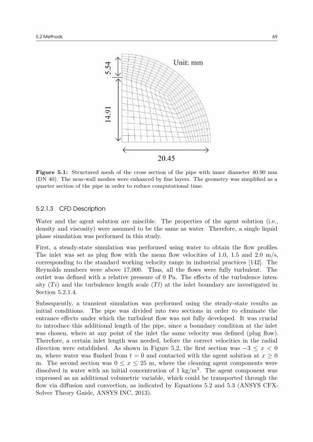
5.2 Methods 69
Figure 5.1: Structured mesh of the cross section of the pipe with inner diameter 40.90 mm(DN 40). The near-wall meshes were enhanced by fine layers. The geometry was simplified as aquarter section of the pipe in order to reduce computational time.
5.2.1.3 CFD Description
Water and the agent solution are miscible. The properties of the agent solution (i.e.,density and viscosity) were assumed to be the same as water. Therefore, a single liquidphase simulation was performed in this study.
First, a steady-state simulation was performed using water to obtain the flow profiles.The inlet was set as plug flow with the mean flow velocities of 1.0, 1.5 and 2.0 m/s,corresponding to the standard working velocity range in industrial practices [142]. TheReynolds numbers were above 17,000. Thus, all the flows were fully turbulent. Theoutlet was defined with a relative pressure of 0 Pa. The effects of the turbulence inten-sity (Ti) and the turbulence length scale (T l) at the inlet boundary are investigated inSection 5.2.1.4.
Subsequently, a transient simulation was performed using the steady-state results asinitial conditions. The pipe was divided into two sections in order to eliminate theentrance effects under which the turbulent flow was not fully developed. It was crucialto introduce this additional length of the pipe, since a boundary condition at the inletwas chosen, where at any point of the inlet the same velocity was defined (plug flow).Therefore, a certain inlet length was needed, before the correct velocities in the radialdirection were established. As shown in Figure 5.2, the first section was −3 ≤ x < 0m, where water was flushed from t = 0 and contacted with the agent solution at x ≥ 0m. The second section was 0 ≤ x ≤ 25 m, where the cleaning agent components weredissolved in water with an initial concentration of 1 kg/m3. The agent component wasexpressed as an additional volumetric variable, which could be transported through theflow via diffusion and convection, as indicated by Equations 5.2 and 5.3 (ANSYS CFX-Solver Theory Guide, ANSYS INC, 2013).
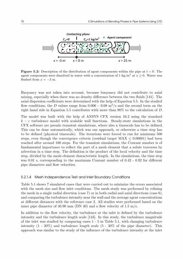
70 5 Simulations of Blending Phases in Pipe Systems Using CFD
Figure 5.2: Description of the distribution of agent components within the pipe at t = 0. Theagent components were dissolved in water with a concentration of 1 kg/m3 at x ≥ 0. Water wasflushed from x = −3 m.
Buoyancy was not taken into account, because buoyancy did not contribute to axialmixing, especially when there was no density difference between the two fluids [141]. Theaxial dispersion coefficients were determined with the help of Equation 5.5. In the studiedflow conditions, the D values range from 0.006 − 0.08 m2/s and the second term on theright hand side in Equation 5.5 contributes with more than 90% to the calculation of D.
The model was built with the help of ANSYS CFX version 16.2 using the standardk − ε turbulence model with scalable wall functions. Steady-state simulations in theCFX software are pseudo transient simulations, where also a timescale has to be defined.This can be done automatically, which was our approach, or otherwise a time step hasto be defined (physical timescale). The iterations were forced to run for minimum 500steps, even though the convergence criteria (residual target MAX ≤ 0.00001) had beenreached after around 100 steps. For the transient simulations, the Courant number is offundamental importance to reflect the part of a mesh element that a solute traverses byadvection in a time step. The definition is the product of the local velocity and the timestep, divided by the mesh element characteristic length. In the simulations, the time stepwas 0.01 s, corresponding to the maximum Courant number of 0.42 - 0.92 for differentpipe diameters and flow velocities.
5.2.1.4 Mesh Independence Test and Inlet Boundary Conditions
Table 5.1 shows 7 simulated cases that were carried out to minimize the errors associatedwith the mesh size and flow inlet conditions. The mesh study was performed by refiningthe mesh in a single radial direction (case 7) or in both radial and axial directions (case 6),and comparing the turbulence intensity near the wall and the average agent concentrationsat different distances with the reference case 2. All studies were performed based on theinner pipe diameter of 40.90 mm (DN 40) and a flow velocity of 1.5 m/s.
In addition to the flow velocity, the turbulence at the inlet is defined by the turbulenceintensity and the turbulence length scale [143]. In this study, the turbulence magnitudeof the inlet was studied by comparing cases 1 - 5 in Table 5.1, with changing turbulenceintensity (1 - 20%) and turbulence length scale (5 - 30% of the pipe diameter). Thisapproach was similar to the study of the influence of the turbulence intensity at the inlet

5.2 Methods 71
Table 5.1: Parameters for the mesh study and for the influence of the turbulence intensity andthe turbulence length scale. The inner pipe diameter is 40.90 mm (DN 40), the flow velocity is1.5 m/s. Case 2 is the reference case that is selected for the following studies.
Case Meshindexes
No. of nodesin radial/axial
directions
Tib,[%]
T lb, [% ofdiameter] y+
Max.CourantNumber
MeanCourantnumber
1 Mesh 1 21/501 1 10 45 0.69 0.262 Mesh 1 21/501 5 10 45 0.69 0.263 Mesh 1 21/501 20 10 45 0.70 0.264 Mesh 1 21/501 5 5 45 0.69 0.265 Mesh 1 21/501 5 30 45 0.69 0.266 Mesh 2 29/751 5 10 32 1.04 0.397 Mesh 3 27/501 5 10 4 0.81 0.24
on wall shear stress fluctuations by Jensen (2007) [144].
5.2.2 Simulation of Complex Geometries
5.2.2.1 Geometries and Model Description
The complex geometries studied are listed in Table 5.2, including dimensions. The simula-tions of these geometries were designed as assignments in a CFD course with 24 attendees(either master or Ph.D students). Each geometry was chosen by at least one student andseveral geometries were modelled by two students.
Similar simulation approaches as straight pipes were performed but simplified for complexgeometries. The investigated flow velocities were 1.5 or 3.0 m/s. The entrance lengthto eliminate any inlet effect was 10 times the inlet diameter instead of 3 m length forstraight pipes. The outlet was placed 0.2 m downstream of the studied volume with astatic pressure of 0 Pa. The axial dispersion coefficient through Equation 5.5 only appliesto straight pipes where the Reynolds numbers are the same in different axial distances.However, for complex geometries, the values of the axial dispersion coefficient vary atdifferent locations. Therefore, the dispersion coefficient in Equation 5.3 was obtained bydefining the molecular diffusion coefficient D0 = 1·10−9 m2 s-1 and the turbulent Schmidtnumber Sct = 0.7 referring to the works done by others [141].
5.2.2.2 Calculation of Pressure Drop
The pressure drop is another critical characteristic parameter for describing the cleaningperformance of long and complex pipe systems. A large pressure drop results in substan-tial power consumption to transfer the cleaning fluids. In the analytical approach, thefollowing Bernoulli equation describes the impulse balance:
u12
2g+ P1
ρg+ z1 = u2
2
2g+ P2
ρg+ z2 + △hl 5.6
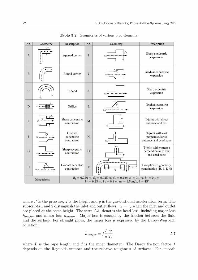
72 5 Simulations of Blending Phases in Pipe Systems Using CFD
Table 5.2: Geometries of various pipe elements.
where P is the pressure, z is the height and g is the gravitational acceleration term. Thesubscripts 1 and 2 distinguish the inlet and outlet flows. z1 = z2 when the inlet and outletare placed at the same height. The term △hl denotes the head loss, including major losshmajor and minor loss hminor. Major loss is caused by the friction between the fluidand the surface. For straight pipes, the major loss is expressed by the Darcy-Weisbachequation:
hmajor = fL
d
u2
2g5.7
where L is the pipe length and d is the inner diameter. The Darcy friction factor fdepends on the Reynolds number and the relative roughness of surfaces. For smooth
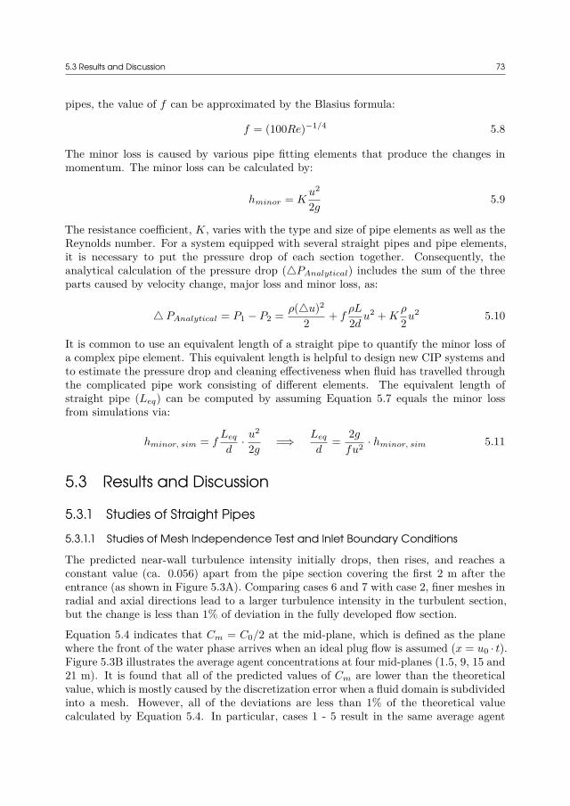
5.3 Results and Discussion 73
pipes, the value of f can be approximated by the Blasius formula:
f = (100Re)−1/4 5.8
The minor loss is caused by various pipe fitting elements that produce the changes inmomentum. The minor loss can be calculated by:
hminor = Ku2
2g5.9
The resistance coefficient, K, varies with the type and size of pipe elements as well as theReynolds number. For a system equipped with several straight pipes and pipe elements,it is necessary to put the pressure drop of each section together. Consequently, theanalytical calculation of the pressure drop (△PAnalytical) includes the sum of the threeparts caused by velocity change, major loss and minor loss, as:
△ PAnalytical = P1 − P2 = ρ(△u)2
2+ f
ρL
2du2 + K
ρ
2u2 5.10
It is common to use an equivalent length of a straight pipe to quantify the minor loss ofa complex pipe element. This equivalent length is helpful to design new CIP systems andto estimate the pressure drop and cleaning effectiveness when fluid has travelled throughthe complicated pipe work consisting of different elements. The equivalent length ofstraight pipe (Leq) can be computed by assuming Equation 5.7 equals the minor lossfrom simulations via:
hminor, sim = fLeq
d· u2
2g=⇒ Leq
d= 2g
fu2 · hminor, sim 5.11
5.3 Results and Discussion
5.3.1 Studies of Straight Pipes5.3.1.1 Studies of Mesh Independence Test and Inlet Boundary Conditions
The predicted near-wall turbulence intensity initially drops, then rises, and reaches aconstant value (ca. 0.056) apart from the pipe section covering the first 2 m after theentrance (as shown in Figure 5.3A). Comparing cases 6 and 7 with case 2, finer meshes inradial and axial directions lead to a larger turbulence intensity in the turbulent section,but the change is less than 1% of deviation in the fully developed flow section.
Equation 5.4 indicates that Cm = C0/2 at the mid-plane, which is defined as the planewhere the front of the water phase arrives when an ideal plug flow is assumed (x = u0 · t).Figure 5.3B illustrates the average agent concentrations at four mid-planes (1.5, 9, 15 and21 m). It is found that all of the predicted values of Cm are lower than the theoreticalvalue, which is mostly caused by the discretization error when a fluid domain is subdividedinto a mesh. However, all of the deviations are less than 1% of the theoretical valuecalculated by Equation 5.4. In particular, cases 1 - 5 result in the same average agent

74 5 Simulations of Blending Phases in Pipe Systems Using CFD
Figure 5.3: (A) Near-wall turbulence intensity (1 mm from the wall) and (B) average agentconcentration at various mid-planes for different model cases. The inner pipe diameter is 40.90mm (DN 40), the flow velocity is 1.5 m/s. The parameters for different cases are shown inTable 5.1.
concentration values (with precision 0.00001 kg/m3) at the four mid-planes. Therefore,it can be concluded from Figure 5.3 that the differences caused by mesh sizes as well asthe turbulence intensity and turbulence length scale are only limited to the initial 2 mpipe section, but are no longer observable from x = 0.
Hence, case 2 provides a sufficient mesh for this project. Extremely fine meshes likecases 6 and 7 may be counter-productive, because the mixing in the radial directionis not significant (see Figure 5.7) and flat mesh elements lead to low mesh quality inslender pipes. The results imply that the use of a 3 m pipe as entrance (Figure 5.2), is areasonable measure to overcome the effects of entrance fluctuations. The meshes of otherpipe diameters were made by fixing axial nodes similar to case 2 and adjusting radialnodes to result in identical layer size and y+. The value of y+ describes how coarse orfine of a mesh is at the boundary, a large value of which normally indicates a relativelycoarse mesh and vice versa. The inlet boundary conditions are selected to Ti = 5% andT l = 10% of the pipe diameter. When a new mesh and a new flow velocity were employed,the same validation approaches as demonstrated in Figure 5.3 were carried out in orderto ensure that the flow was in a turbulent condition at x = 0 and Cm ≈ 0.5C0 at themid-planes.
5.3.1.2 Comparison of the Taylor Model and CFD Simulations
Figure 5.4 shows the agent concentrations at the mean flow velocity of 1.5 m/s at x = 15m and for a fixed rinsing time (10 s) at an arbitrary distance. The presented valuesare obtained from the Taylor model [139] and the CFD simulations. Figure 5.4A canbe regarded as the displacement dynamics at the fixed plane during the rinsing period.Figure 5.4B can be considered as the agent distributions within the pipe after 10 s ofrinsing.

5.3 Results and Discussion 75
Figure 5.4: Comparison of the Taylor model and the CFD simulations at 1.5 m/s of flowvelocity for (A) a fixed distance of 15 m with varied rinsing time, and (B) a fixed rinsing timeof 10 s with varied distance.
The agent components transfer slower near the wall than in the center due to bluntvelocity profiles (Figure 5.5). The longer tails in larger pipes (Figure 5.4) indicate thatthe agent components are axially mixed faster in the pipe center but slower near thewall than in smaller pipes. The mixing of agent molecules is a result of convection anddiffusion [137]. According to Equation 5.5, the value of the axial dispersion coefficientincreases with increasing pipe diameter when the flow is turbulent [138]. In Figure 5.5,the value of turbulent kinetic energy k is minimal at the center and increases towardsthe radial direction, and decreases near the wall, which is the same as Zhao et al. (2010)observed when simulating the mixing of two miscible liquids with different densities [141].Considering the lower center velocity but larger axial diffusion for larger pipes, it can beconcluded that the mixing of the agent components is governed by axial diffusion in thepipe center section, and by convection near the wall.
CFD successfully predicts the values which are calculated with help of the Taylor model[139]. The CFD model predicts accurately the analytical model in terms of the tran-sient agent concentrations at different locations in the pipe. In addition to the Taylormodel, the prediction of dispersion within a pipe by using CFD has also been verifiedto be successful by predicting Stegowski et al. (2013)’s experimental data [145] and theresidence time distribution (RTD) theory [146]. The validations of the latter two ap-proaches are provided in the supplementary material in Yang et al. (2018) [134] (DOI:10.1016/j.jfoodeng.2017.09.017), which are not shown in this thesis. Therefore, the CFDmodel is used for further investigations of the displacement process and the mixing zoneanalysis.
5.3.1.3 Displacement Time
Three displacement times are defined in this work for different purposes:
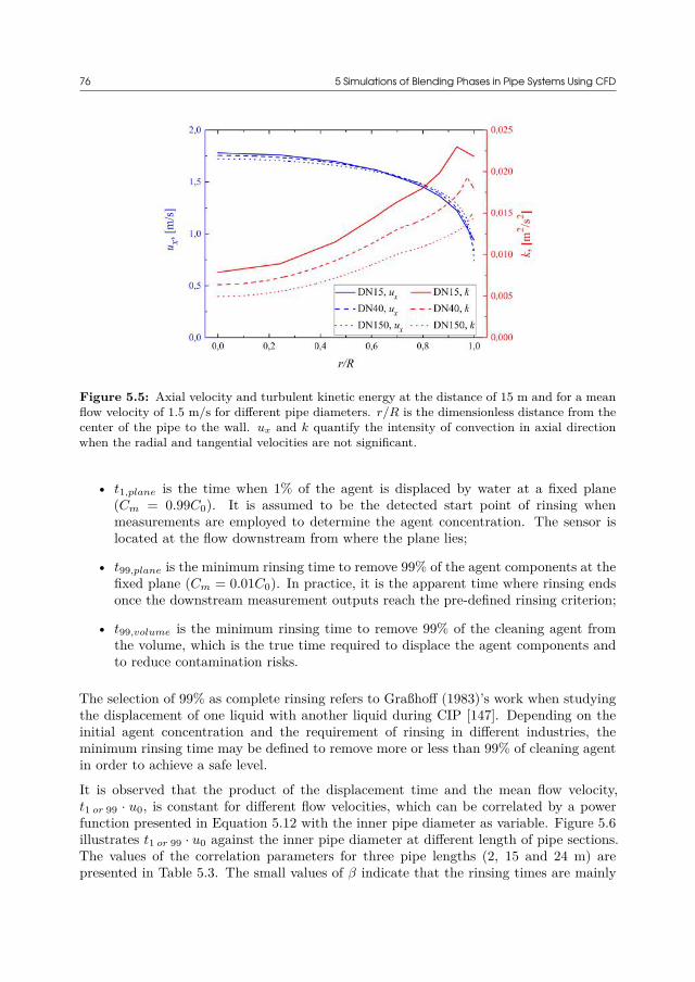
76 5 Simulations of Blending Phases in Pipe Systems Using CFD
Figure 5.5: Axial velocity and turbulent kinetic energy at the distance of 15 m and for a meanflow velocity of 1.5 m/s for different pipe diameters. r/R is the dimensionless distance from thecenter of the pipe to the wall. ux and k quantify the intensity of convection in axial directionwhen the radial and tangential velocities are not significant.
• t1,plane is the time when 1% of the agent is displaced by water at a fixed plane(Cm = 0.99C0). It is assumed to be the detected start point of rinsing whenmeasurements are employed to determine the agent concentration. The sensor islocated at the flow downstream from where the plane lies;
• t99,plane is the minimum rinsing time to remove 99% of the agent components at thefixed plane (Cm = 0.01C0). In practice, it is the apparent time where rinsing endsonce the downstream measurement outputs reach the pre-defined rinsing criterion;
• t99,volume is the minimum rinsing time to remove 99% of the cleaning agent fromthe volume, which is the true time required to displace the agent components andto reduce contamination risks.
The selection of 99% as complete rinsing refers to Graßhoff (1983)’s work when studyingthe displacement of one liquid with another liquid during CIP [147]. Depending on theinitial agent concentration and the requirement of rinsing in different industries, theminimum rinsing time may be defined to remove more or less than 99% of cleaning agentin order to achieve a safe level.
It is observed that the product of the displacement time and the mean flow velocity,t1 or 99 · u0, is constant for different flow velocities, which can be correlated by a powerfunction presented in Equation 5.12 with the inner pipe diameter as variable. Figure 5.6illustrates t1 or 99 · u0 against the inner pipe diameter at different length of pipe sections.The values of the correlation parameters for three pipe lengths (2, 15 and 24 m) arepresented in Table 5.3. The small values of β indicate that the rinsing times are mainly
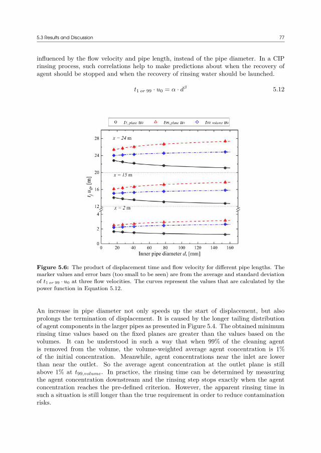
5.3 Results and Discussion 77
influenced by the flow velocity and pipe length, instead of the pipe diameter. In a CIPrinsing process, such correlations help to make predictions about when the recovery ofagent should be stopped and when the recovery of rinsing water should be launched.
t1 or 99 · u0 = α · dβ 5.12
Figure 5.6: The product of displacement time and flow velocity for different pipe lengths. Themarker values and error bars (too small to be seen) are from the average and standard deviationof t1 or 99 · u0 at three flow velocities. The curves represent the values that are calculated by thepower function in Equation 5.12.
An increase in pipe diameter not only speeds up the start of displacement, but alsoprolongs the termination of displacement. It is caused by the longer tailing distributionof agent components in the larger pipes as presented in Figure 5.4. The obtained minimumrinsing time values based on the fixed planes are greater than the values based on thevolumes. It can be understood in such a way that when 99% of the cleaning agentis removed from the volume, the volume-weighted average agent concentration is 1%of the initial concentration. Meanwhile, agent concentrations near the inlet are lowerthan near the outlet. So the average agent concentration at the outlet plane is stillabove 1% at t99,volume. In practice, the rinsing time can be determined by measuringthe agent concentration downstream and the rinsing step stops exactly when the agentconcentration reaches the pre-defined criterion. However, the apparent rinsing time insuch a situation is still longer than the true requirement in order to reduce contaminationrisks.

78 5 Simulations of Blending Phases in Pipe Systems Using CFD
Table 5.3: Correlation parameters of the product of displacement time and flow velocity forthree pipe lengths by the power function as Equation 5.12. The unit of inner pipe diametershould be meter.
x, [m] t, [s] α, [m1-β ] β R2
2t1,plane 1.01 -0.121 0.998t99,plane 3.83 0.107 0.963
t99,volume 3.03 0.0788 0.966
15t1,plane 11.7 -0.0456 0.989t99,plane 19.1 0.0422 0.978
t99,volume 16.4 0.0212 0.970
24t1,plane 19.8 -0.0354 0.996t99,plane 29.1 0.0337 0.980
t99,volume 25.5 0.0152 0.971
5.3.1.4 Minimum Water Consumption for Rinsing
The minimum water consumption for an effective rinsing is the minimum requirementof water to reduce the amount of agent to such a low degree that the residues haveno or only a minor effect on the following steps. In this study, the removal of 99% ofagent components is assumed as a complete rinse. In order to compare the minimumconsumption for different pipe diameters, a volume factor, F , is defined as the ratiobetween the minimum water consumption, Vmin, and the pipe volume, V , as follows:
F = Vmin
V= πd2/4 · u0 · tmin
πd2/4 · x= u0 · t99
x5.13
Equation 5.12 indicates that the value of u0 · t99 only depends on the inner pipe diameterfor a given pipe length. Therefore, according to Equation 5.13, the values of volumefactors are independent of flow velocities as well. The increase in flow velocity reducesthe rinsing time significantly, but it does not affect the minimum water consumption.However, if water also works as a medium to remove soils from surfaces, large flow ve-locities improve rinsing efficiency by destroying the structure between soils and surfacesby mechanical forces, i.e., shear stress [6]. The pipes of larger size lead to larger volumefactors, as t99 increases with increasing inner pipe diameters. Both the numerator anddenominator in Equation 5.13 increase for longer pipes, but the value of u0 · t99 growsslower than x. Thus, the volume factors become smaller for longer pipes.
With decreasing pipe diameter and increasing pipe length, the volume factor values tendto the lower limit of 1, indicating that the minimum water consumption approaches thepipe volume. It can also be concluded that the calculated volume factors based on thedownstream measurement are larger than the values based on the volume, which is thesame trend as the illustrated rinsing time in Figure 5.6. Therefore, if the rinsing time iscontrolled by downstream measurements, the consumption of water is still 6 - 20% largerthan the real demand to remove a certain amount of agent from the volume.
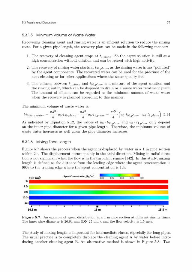
5.3 Results and Discussion 79
5.3.1.5 Minimum Volume of Waste Water
Recovering cleaning agent and rinsing water is an efficient solution to reduce the rinsingcosts. For a given pipe length, the recovery plan can be made in the following manner:
1. The recovery of cleaning agent stops at t1,plane. So the agent solution is still at ahigh concentration without dilution and can be reused with high activity;
2. The recovery of rinsing water starts at t99,plane, as the rinsing water is less “polluted”by the agent components. The recovered water can be used for the pre-rinse of thenext cleaning or for other applications where the water quality fits;
3. The effluent between t1,plane and t99,plane is a mixture of the agent solution andthe rinsing water, which can be disposed to drain or a waste water treatment plant.The amount of effluent can be regarded as the minimum amount of waste waterwhen the recovery is planned according to this manner.
The minimum volume of waste water is:
VW aste water = πd2
4·u0 ·t99,plane− πd2
4·u0 ·t1,plane = πd2
4·(
u0 ·t99,plane−u0 ·t1,plane
)5.14
As indicated by Equation 5.12, the values of u0 · t99,plane and u0 · t1,plane only dependon the inner pipe diameter for a given pipe length. Therefore, the minimum volume ofwaste water increases as well when the pipe diameter increases.
5.3.1.6 Mixing Zone Length
Figure 5.7 shows the process when the agent is displaced by water in a 1 m pipe sectionwithin 2 s. The displacement occurs mainly in the axial direction. Mixing in radial direc-tion is not significant when the flow is in the turbulent regime [142]. In this study, mixinglength is defined as the distance from the leading edge where the agent concentration is99% to the trailing edge where the agent concentration is 1%.
Figure 5.7: An example of agent distribution in a 1 m pipe section at different rinsing times.The inner pipe diameter is 26.64 mm (DN 25 mm), and the flow velocity is 1.5 m/s.
The study of mixing length is important for intermediate rinses, especially for long pipes.The usual practice is to completely displace the cleaning agent A by water before intro-ducing another cleaning agent B. An alternative method is shown in Figure 5.8. Two
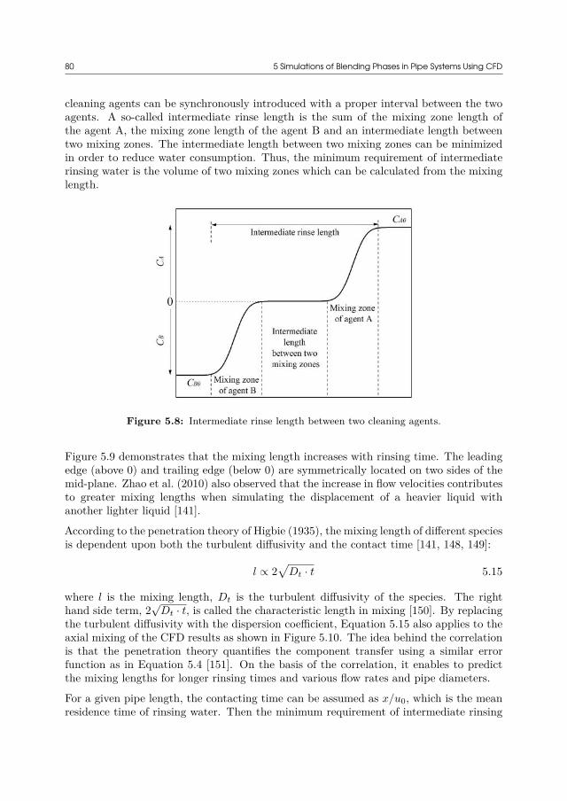
80 5 Simulations of Blending Phases in Pipe Systems Using CFD
cleaning agents can be synchronously introduced with a proper interval between the twoagents. A so-called intermediate rinse length is the sum of the mixing zone length ofthe agent A, the mixing zone length of the agent B and an intermediate length betweentwo mixing zones. The intermediate length between two mixing zones can be minimizedin order to reduce water consumption. Thus, the minimum requirement of intermediaterinsing water is the volume of two mixing zones which can be calculated from the mixinglength.
Figure 5.8: Intermediate rinse length between two cleaning agents.
Figure 5.9 demonstrates that the mixing length increases with rinsing time. The leadingedge (above 0) and trailing edge (below 0) are symmetrically located on two sides of themid-plane. Zhao et al. (2010) also observed that the increase in flow velocities contributesto greater mixing lengths when simulating the displacement of a heavier liquid withanother lighter liquid [141].
According to the penetration theory of Higbie (1935), the mixing length of different speciesis dependent upon both the turbulent diffusivity and the contact time [141, 148, 149]:
l ∝ 2√
Dt · t 5.15
where l is the mixing length, Dt is the turbulent diffusivity of the species. The righthand side term, 2
√Dt · t, is called the characteristic length in mixing [150]. By replacing
the turbulent diffusivity with the dispersion coefficient, Equation 5.15 also applies to theaxial mixing of the CFD results as shown in Figure 5.10. The idea behind the correlationis that the penetration theory quantifies the component transfer using a similar errorfunction as in Equation 5.4 [151]. On the basis of the correlation, it enables to predictthe mixing lengths for longer rinsing times and various flow rates and pipe diameters.
For a given pipe length, the contacting time can be assumed as x/u0, which is the meanresidence time of rinsing water. Then the minimum requirement of intermediate rinsing
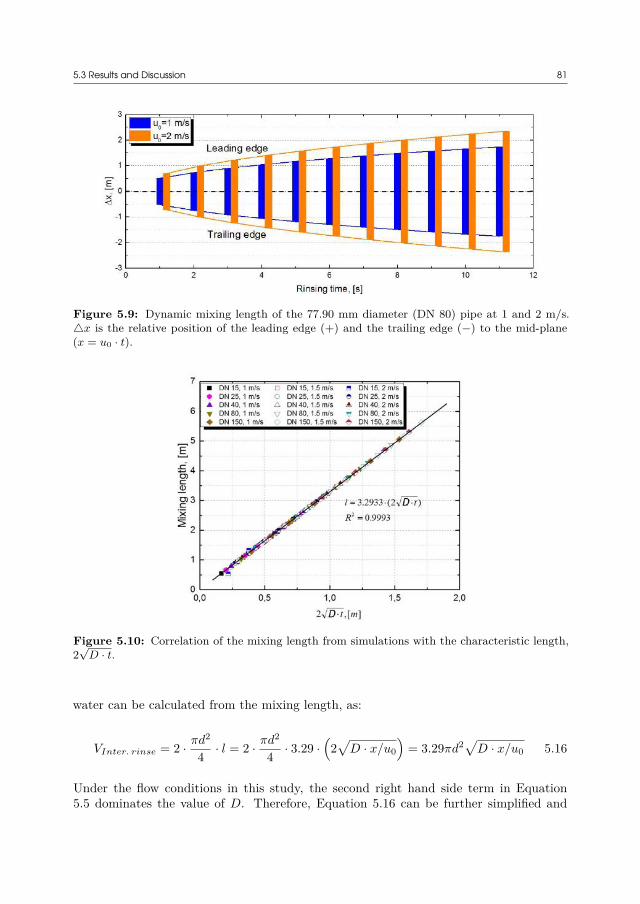
5.3 Results and Discussion 81
Figure 5.9: Dynamic mixing length of the 77.90 mm diameter (DN 80) pipe at 1 and 2 m/s.△x is the relative position of the leading edge (+) and the trailing edge (−) to the mid-plane(x = u0 · t).
Figure 5.10: Correlation of the mixing length from simulations with the characteristic length,2√
D · t.
water can be calculated from the mixing length, as:
VInter. rinse = 2 · πd2
4· l = 2 · πd2
4· 3.29 ·
(2√
D · x/u0
)= 3.29πd2
√D · x/u0 5.16
Under the flow conditions in this study, the second right hand side term in Equation5.5 dominates the value of D. Therefore, Equation 5.16 can be further simplified and

82 5 Simulations of Blending Phases in Pipe Systems Using CFD
approximated as:
VInter. rinse ≈ 3.29πd2√
1.35(u0d)0.875 · (µ/ρ)0.125 · x/u0
= 3.82π√
u0.3750 d4.875(µ/ρ)0.125x
5.17
5.3.2 Studies of Complex GeometriesThe studies of complex geometries include two scenarios: (i) When water is the cleaningmedium to detach soil materials from the surfaces, dead zones indicate the locationsthat are the most difficult to clean. These dead zones result in higher pressure dropsthan straight pipes. The identification of dead zones and the computation of pressuredrops are achieved by the steady state simulations. (ii) When water is used to displacecleaning agents from the pipe fittings, which is the same as the studies of straight pipes,the minimum rinsing time and minimum water consumption can be obtained from thetransient simulation results.
5.3.2.1 Dead Zone Identification
In cleaning operations, the removal of soil components from surfaces is insufficient whenthe local wall shear stress is below a critical value of 3 Pa [45]. Figure 5.11 shows an exam-ple of the predicted WSS of the complex geometry P (see Table 5.2) in comparison withthe corresponding individual elements. The predicted WSS values for other geometriesare provided in Appendix A. A number of conclusions can be drawn from the findings:
Figure 5.11: Predicted wall shear stress on the surfaces of five geometries.
• The extrados surface and the intrados surface of bends (see Figure 5.11) as well asboth sides of orifices are difficult to clean. Furthermore, the dead zones also includethe large pipe corners of contractions, the large pipe and connection of expansions,
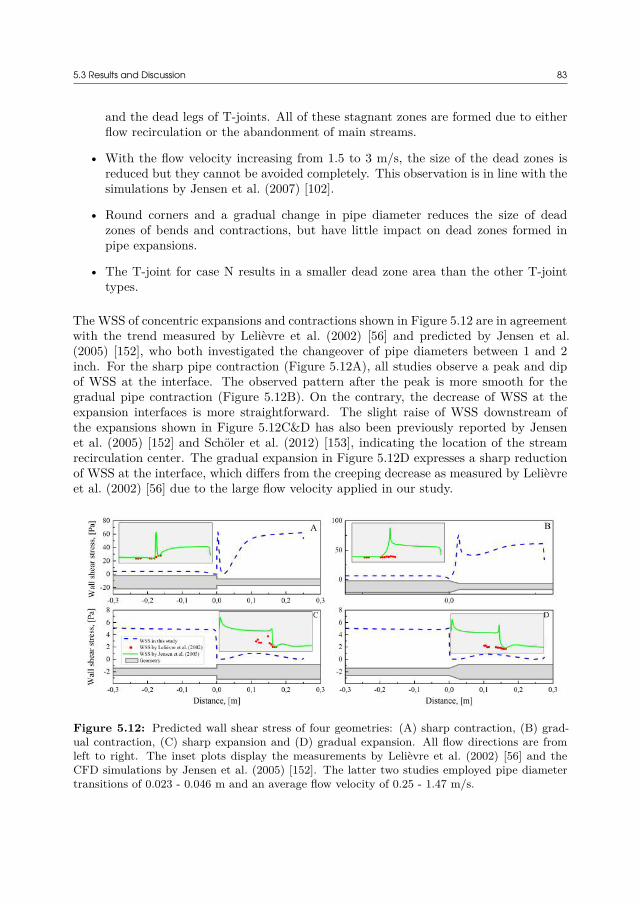
5.3 Results and Discussion 83
and the dead legs of T-joints. All of these stagnant zones are formed due to eitherflow recirculation or the abandonment of main streams.
• With the flow velocity increasing from 1.5 to 3 m/s, the size of the dead zones isreduced but they cannot be avoided completely. This observation is in line with thesimulations by Jensen et al. (2007) [102].
• Round corners and a gradual change in pipe diameter reduces the size of deadzones of bends and contractions, but have little impact on dead zones formed inpipe expansions.
• The T-joint for case N results in a smaller dead zone area than the other T-jointtypes.
The WSS of concentric expansions and contractions shown in Figure 5.12 are in agreementwith the trend measured by Lelièvre et al. (2002) [56] and predicted by Jensen et al.(2005) [152], who both investigated the changeover of pipe diameters between 1 and 2inch. For the sharp pipe contraction (Figure 5.12A), all studies observe a peak and dipof WSS at the interface. The observed pattern after the peak is more smooth for thegradual pipe contraction (Figure 5.12B). On the contrary, the decrease of WSS at theexpansion interfaces is more straightforward. The slight raise of WSS downstream ofthe expansions shown in Figure 5.12C&D has also been previously reported by Jensenet al. (2005) [152] and Schöler et al. (2012) [153], indicating the location of the streamrecirculation center. The gradual expansion in Figure 5.12D expresses a sharp reductionof WSS at the interface, which differs from the creeping decrease as measured by Lelièvreet al. (2002) [56] due to the large flow velocity applied in our study.
Figure 5.12: Predicted wall shear stress of four geometries: (A) sharp contraction, (B) grad-ual contraction, (C) sharp expansion and (D) gradual expansion. All flow directions are fromleft to right. The inset plots display the measurements by Lelièvre et al. (2002) [56] and theCFD simulations by Jensen et al. (2005) [152]. The latter two studies employed pipe diametertransitions of 0.023 - 0.046 m and an average flow velocity of 0.25 - 1.47 m/s.

84 5 Simulations of Blending Phases in Pipe Systems Using CFD
5.3.2.2 Pressure Drop
The simulated pressure drops from inlet to outlet generated in the steady-state simulationswere extracted in comparison with the analytical pressure drops by taking K values fromTable 5.4 applied in Equation 5.9. According to Figure 5.13, the simulated pressure dropsfollow the same trend as the values based on the analytical approaches, with most of thefigures in less than 50% or 30% of deviation. The most uncertainty of the analyticalresults comes from the determination of K, the value of which was obtained empiricallyin literature for specific types of pipe elements and flow conditions. Furthermore, the Kvalues are derived based on stable flow profiles, where for instance the turbulence has beenfully developed downstream of contractions or expansions. However, in some simulationcases (i.g., geometries I, J, K and L), the reserved length prior to the outlet is not longenough to establish stability. Thus, the resulted values of △PSim differ from the expectedanalytical solutions. However, the absolute pressure drops for these geometries are lessthan 103 Pa, meaning the high variation of these points displayed in the logarithmic plotin Figure 5.13 actually contains only minor absolute deviations.
Table 5.4: The resistance coefficient values, K, for different pipe elements
No. K Sources No. K Sources
A 1.2 3-K model by Darbyet al. (2017) [154]
I 0.6Sudden expansion modelby Rennels et al. (2012)
[155]
B 0.4 J 0.6Gradual expansion model
by Darby et al. (2017)[154]
C 0.5 K 1.0 2-K model for exit byDarby et al. (2017) [154]
D 32.7 2-K model by Darby et al.(2017) [154] L 0.7
15% higher than concentricexpansion, according to
Rennels et al. (2012) [155]
E 7.3 Sudden contraction modelby Neutrium (2012) [156] M 0.2 Flanged tee for line flow by
Young et al. (2010) [157]
F 6.1Gradual contraction model
by Darby et al. (2017)[154]
N 1.0 Flanged tee for branchflow by Young et al.
(2010) [157]G 1.0 2-K model for entrance by
Darby et al. (2017) [154] O 1.0
H 4.9
Contraction model byDarby et al. (2017) [154]
with equivalent anglecalculated by Rennels et al.
(2012) [155]
P 9.3 Sum of K values forgeometries B, E, I, N
The equivalent lengths of different pipe elements are displayed in Figure 5.14. It needsto be mentioned that the values of equivalent lengths depend significantly on the element
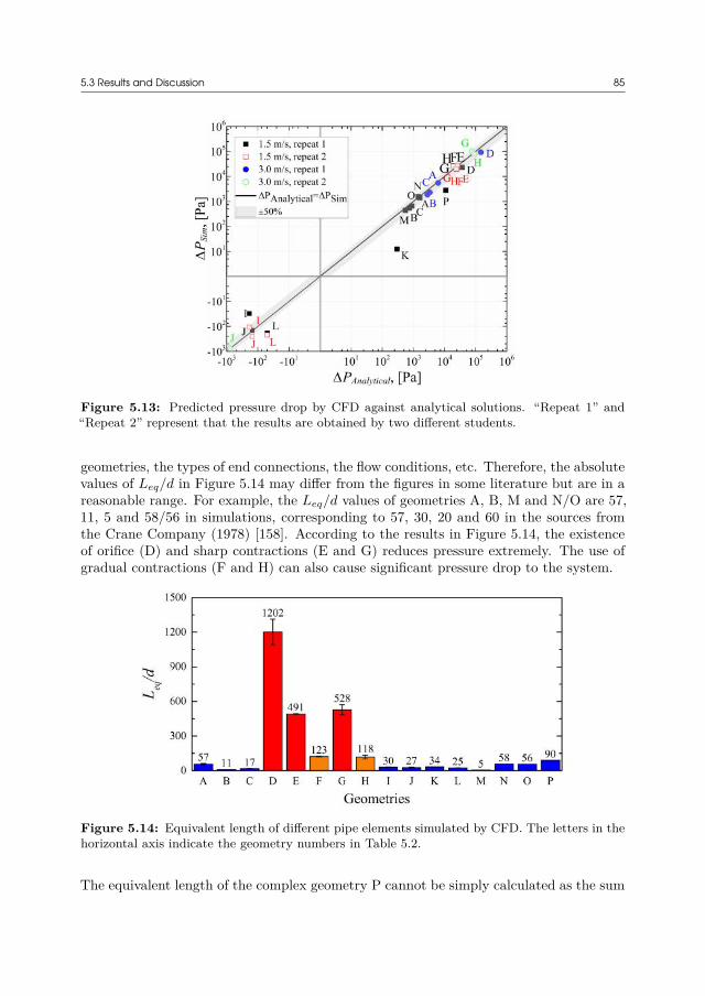
5.3 Results and Discussion 85
Figure 5.13: Predicted pressure drop by CFD against analytical solutions. “Repeat 1” and“Repeat 2” represent that the results are obtained by two different students.
geometries, the types of end connections, the flow conditions, etc. Therefore, the absolutevalues of Leq/d in Figure 5.14 may differ from the figures in some literature but are in areasonable range. For example, the Leq/d values of geometries A, B, M and N/O are 57,11, 5 and 58/56 in simulations, corresponding to 57, 30, 20 and 60 in the sources fromthe Crane Company (1978) [158]. According to the results in Figure 5.14, the existenceof orifice (D) and sharp contractions (E and G) reduces pressure extremely. The use ofgradual contractions (F and H) can also cause significant pressure drop to the system.
Figure 5.14: Equivalent length of different pipe elements simulated by CFD. The letters in thehorizontal axis indicate the geometry numbers in Table 5.2.
The equivalent length of the complex geometry P cannot be simply calculated as the sum

86 5 Simulations of Blending Phases in Pipe Systems Using CFD
of the equivalent lengths of the simple geometries B, E, I and N. The reason is that thepipe elements in the proposed geometry P are located so close to each other that the flowpattern differs from the cases where single elements are simulated.
The CFD approach is an effective method to investigate the pressure drop occurring inpipe systems. The analytical equation can only quantify the total pressure drop, whileCFD can result in additional information such as the flow pattern and pressure gradientin cross sections. For future applications, the roughness of the pipe surface can be addedto the model, with the friction factor obtained from the Moody chart. This roughnessterm can also be implemented in CFD codes.
5.3.2.3 Displacement Time
Figure 5.15 displays the predicted values of t99,volume and t99,point for different pipe ele-ments. t99,point is defined as the time to displace 99% cleaning agent from a point locatedin the dead volume determined previously. According to the result, bends and contrac-tions are easy to be rinsed, except the sharp eccentric contraction geometry (G). Pipeexpansions, orifices and T-joint N are comparably hard to be flushed. T-joints M and Oas well as the gradual eccentric expansion (L) are the most difficult to flush. For mostgeometries, the point-based displacement times are larger than the volume-based values,meaning that determining the displacement time by a local sensor is a safe way to validatethe removal of a soluble agent component but causes slightly excessive waste. For thegeometries B, G and H, a measurement-based displacement time is inadequate to reducethe overall agent concentration to a safe level. Moreover, a higher flow velocity shortensthe displacement time significantly. However, the accuracy of the simulations performedby the students needs to be validated using experimental data, even though most repli-cated simulations performed by different students are quite similar. The location of theselected monitoring point is random, which proves to greatly affect the determination oft99,point.
Graßhoff (1980) measured the displacement time to expel 99% of agent components fromthree types of T-joints of the same diameter as in this chapter, using a conductometricelectrode installed at the end of the dead legs [159]. Table 5.5 shows that the predicteddisplacement times are in agreement with the range of experimental results except forgeometry N. This deviation is mostly caused by the limitation of the standard k−ε modelto deal with strong recirculation flows within geometry N.
Figure 5.16 expresses the displacement process within the geometry P. The agent com-ponents at the round corner are displaced very fast. The pipe contraction can also beflushed after about 5 s. However, the agent components in the T-joint and particularlyin the sharp expansion are difficult to be flushed. This trend agrees well with the simula-tions of the individual pipe elements as shown in Figure 5.15. However, the values of thedisplacement times differ due to the change of the flow patterns in the complex geometryP. The result indicates that the determination of rinsing end based on a local sensor atthe T-joint (as shown in the top left graph of Figure 5.16) can give a false “clean” signalafter about 10 s by ignoring the unremoved components in the upstream pipe transition.
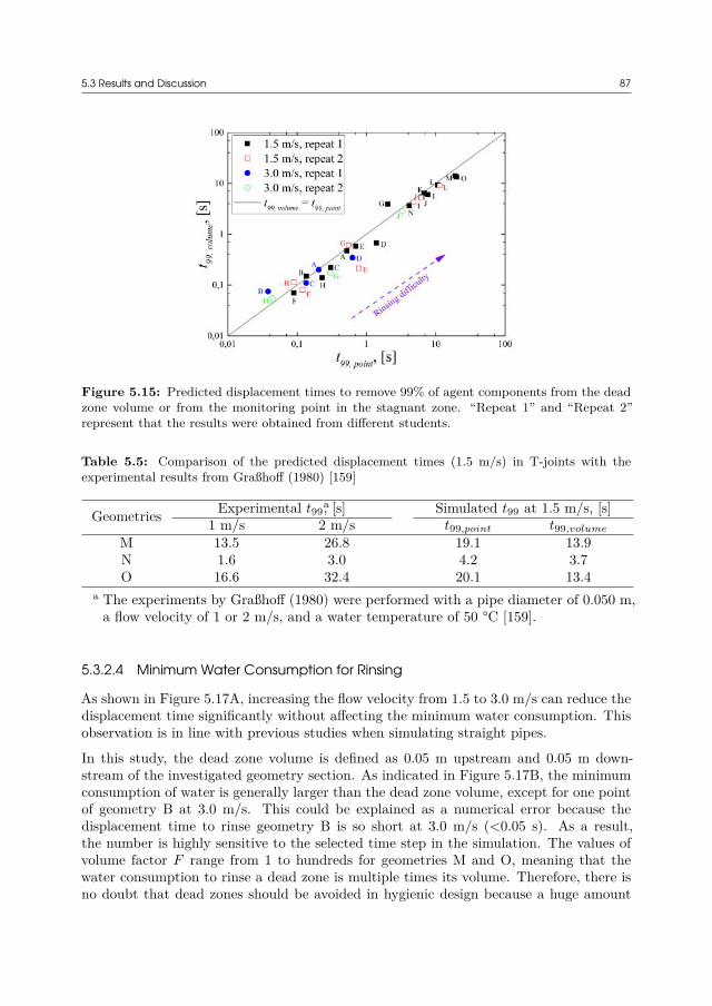
5.3 Results and Discussion 87
Figure 5.15: Predicted displacement times to remove 99% of agent components from the deadzone volume or from the monitoring point in the stagnant zone. “Repeat 1” and “Repeat 2”represent that the results were obtained from different students.
Table 5.5: Comparison of the predicted displacement times (1.5 m/s) in T-joints with theexperimental results from Graßhoff (1980) [159]
Geometries Experimental t99a, [s] Simulated t99 at 1.5 m/s, [s]
1 m/s 2 m/s t99,point t99,volume
M 13.5 26.8 19.1 13.9N 1.6 3.0 4.2 3.7O 16.6 32.4 20.1 13.4
a The experiments by Graßhoff (1980) were performed with a pipe diameter of 0.050 m,a flow velocity of 1 or 2 m/s, and a water temperature of 50 °C [159].
5.3.2.4 Minimum Water Consumption for Rinsing
As shown in Figure 5.17A, increasing the flow velocity from 1.5 to 3.0 m/s can reduce thedisplacement time significantly without affecting the minimum water consumption. Thisobservation is in line with previous studies when simulating straight pipes.
In this study, the dead zone volume is defined as 0.05 m upstream and 0.05 m down-stream of the investigated geometry section. As indicated in Figure 5.17B, the minimumconsumption of water is generally larger than the dead zone volume, except for one pointof geometry B at 3.0 m/s. This could be explained as a numerical error because thedisplacement time to rinse geometry B is so short at 3.0 m/s (<0.05 s). As a result,the number is highly sensitive to the selected time step in the simulation. The values ofvolume factor F range from 1 to hundreds for geometries M and O, meaning that thewater consumption to rinse a dead zone is multiple times its volume. Therefore, there isno doubt that dead zones should be avoided in hygienic design because a huge amount

88 5 Simulations of Blending Phases in Pipe Systems Using CFD
Figure 5.16: Displacement profiles of geometry P.
Figure 5.17: (A) Predicted water consumption to remove 99% of agent components from thedead zone volume or from the monitoring point in the stagnant zone and (B) predicted volumefactors calculated by the volume-based displacement time and point-based displacement time.“Repeat 1” and “Repeat 2” represent that the results were obtained from different students.
of water is required to flush these parts.
5.4 ConclusionsThe study of pipe rinsing is essential to optimize the cleaning operations and to improvethe recovery of cleaning agent solutions and rinsing water. In this chapter, CFD is usedto simulate the displacement of one water-like cleaning agent by water. The simulations
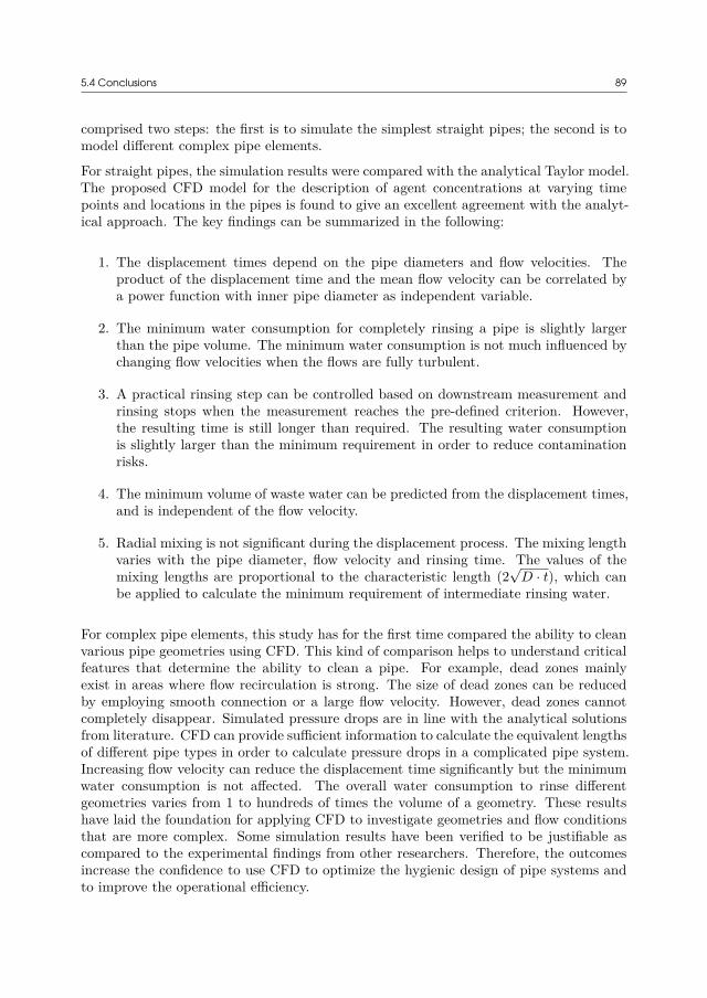
5.4 Conclusions 89
comprised two steps: the first is to simulate the simplest straight pipes; the second is tomodel different complex pipe elements.
For straight pipes, the simulation results were compared with the analytical Taylor model.The proposed CFD model for the description of agent concentrations at varying timepoints and locations in the pipes is found to give an excellent agreement with the analyt-ical approach. The key findings can be summarized in the following:
1. The displacement times depend on the pipe diameters and flow velocities. Theproduct of the displacement time and the mean flow velocity can be correlated bya power function with inner pipe diameter as independent variable.
2. The minimum water consumption for completely rinsing a pipe is slightly largerthan the pipe volume. The minimum water consumption is not much influenced bychanging flow velocities when the flows are fully turbulent.
3. A practical rinsing step can be controlled based on downstream measurement andrinsing stops when the measurement reaches the pre-defined criterion. However,the resulting time is still longer than required. The resulting water consumptionis slightly larger than the minimum requirement in order to reduce contaminationrisks.
4. The minimum volume of waste water can be predicted from the displacement times,and is independent of the flow velocity.
5. Radial mixing is not significant during the displacement process. The mixing lengthvaries with the pipe diameter, flow velocity and rinsing time. The values of themixing lengths are proportional to the characteristic length (2
√D · t), which can
be applied to calculate the minimum requirement of intermediate rinsing water.
For complex pipe elements, this study has for the first time compared the ability to cleanvarious pipe geometries using CFD. This kind of comparison helps to understand criticalfeatures that determine the ability to clean a pipe. For example, dead zones mainlyexist in areas where flow recirculation is strong. The size of dead zones can be reducedby employing smooth connection or a large flow velocity. However, dead zones cannotcompletely disappear. Simulated pressure drops are in line with the analytical solutionsfrom literature. CFD can provide sufficient information to calculate the equivalent lengthsof different pipe types in order to calculate pressure drops in a complicated pipe system.Increasing flow velocity can reduce the displacement time significantly but the minimumwater consumption is not affected. The overall water consumption to rinse differentgeometries varies from 1 to hundreds of times the volume of a geometry. These resultshave laid the foundation for applying CFD to investigate geometries and flow conditionsthat are more complex. Some simulation results have been verified to be justifiable ascompared to the experimental findings from other researchers. Therefore, the outcomesincrease the confidence to use CFD to optimize the hygienic design of pipe systems andto improve the operational efficiency.
90 5 Simulations of Blending Phases in Pipe Systems Using CFD
List of Nomenclature in Chapter 5The following nomenclature is only valid for this chapter. Some symbols are used in otherchapters but with different meanings. Otherwise, the symbols are specifically explainedin the text if there is no nomenclature in some chapter.
Roman LettersC0 Initial agent concentration, [kg m-3]Cm Average agent concentration, [kg m-3]Cµ Model constant for solving the turbulence length scale and the
dissipation rate of turbulence kinetic energy, dimensionlessd Pipe diameter, [m]d1, d2, d3 Dimension of complex geometries, [m]D Dispersion coefficient of species, [m2 s-1]D0 Molecular diffusion coefficient of species, [m2 s-1]Dt Turbulent diffusivity of species, [m2 s-1]f Darcy friction factor, dimensionlessF Volume factor, dimensionlessg Gravity acceleration, [m s-2]hmajor Major loss, [m]hminor Minor loss, [m]H Dimension of complex geometries, [m]J Concentration diffusion flux, [kg m-2 s-1]k Turbulence kinetic energy, [m2 s-2]K Resistance coefficient, dimensionlessl Mixing length, [m]L Pipe length, [m]L1, L2, L3 Dimension of complex geometries, [m]Leq Equivalent length of straight pipe, [m]p Pressure in Navier-Stokes equation, [Pa]P Pressure, [Pa]r Radial coordinate, [m]R Pipe radius, [m]Sct Turbulent Schmidt number, dimensionlesst Time, [s]t1 The time required for displacing 1% of agent by water, [s]t99 The time required for displacing 99% of agent by water, [s]Ti Turbulence intensity, dimensionlessTib Turbulence intensity at inlet, dimensionlessT l Turbulence length scale, [m]T lb Turbulence length scale at inlet, [m]u Flow velocity, [m s-1]u0 Mean flow velocity, [m s-1]ux Axial flow velocity, [m s-1]u′ Fluctuating velocity, [m s-1]V Pipe volume, [m3]
5.4 Conclusions 91
VInter. rinse Volume of intermediate rinsing water, [m3]Vmin Minimum water consumption, [m3]VW astewater Volume of waste water, [m3]x Pipe length, [m]y+ Wall distance for a wall-bound flow, dimensionlessz Height, [m]
Greek Lettersα, β Coefficients correlating the inner pipe diameter and the displace-
ment timeε Dissipation rate of turbulence kinetic energy, [m2 s-3]θ Angle of complex geometry, [°]µ Dynamic viscosity, [Pa s]ν Kinetic viscosity, [Pa s]ρ Density, [kg m-3]

92

CHAPTER6Cleaning of Egg Yolk
Soils from Tank SurfacesUsing Burst Flows
In this chapter, burst techniques have been applied to clean tank surfaces soiled by eggyolk materials. The work was performed in collaboration with Alfa Laval CopenhagenA/S. This chapter of the thesis has been published and reproduced based on the followingarticle [135]:
Investigation of the cleaning of egg yolk deposits from tank surfaces using continuous andpulsed flowsYang, J., Kjellberg, K., Jensen, B. B. B., Nordkvist, M., Gernaey, K. V., Krühne, U.Food and Bioproducts Processing, in pressDOI: 10.1016/j.fbp.2018.10.007
6.1 IntroductionBurst, or pulsed, cleaning in tank cleaning operations is performed by interrupting acontinuous flow with several breaks between the shots of detergent. For tank cleaning,the term burst identifies the rectangular form of a pulse, meaning a two-level outputof a flow rate. In this thesis, Sections 2.1.3 and 2.3 have described the perspectives ofusing burst flows to enhance tank cleaning performance by ensuring surface coverage andproviding additional time for the soaking of soil materials. Consequently, it is anticipatedto save chemical usage and henceforth reduce cleaning costs.
Conventionally, burst tank cleaning is mainly conducted to clean brewery fermenters toremove the foam and yeast deposit that remain on the wall after emptying the tank.In this technique, the water pre-rinse step that is customary in continuous cleaning isskipped. Instead, a burst of alkali solution is applied for wetting the soil layers followedby a pause to allow the detergent to react. This sequence is repeated several times. Ithas been reported that burst cleaning is able to reduce water and chemical consumptionat the expense of longer cleaning time [6, 33, 160]. However, the mechanisms behind theimprovement of tank cleaning by using burst or pulsed flows are still poorly understood,
94 6 Cleaning of Egg Yolk Soils from Tank Surfaces Using Burst Flows
because a standardized method for assessing the performance of tank cleaning is lacking[161].
The scientific literature has discussed how pulsed flows enhance the cleaning of denaturedwhey protein deposits in pipes [162] and annular tube heat exchangers [163]. Reducedchemical consumption was also found by exposing deposits to a chemical environmentbefore water rinse [51]. CFD simulations [102, 164, 165] and the analytical approachesusing Fourier series [166] have proved that the alteration of flow pattern, particularly flowreversal, intensifies the local wall shear stress and hence increases the cleaning efficiency.Furthermore, pulsed flow has been observed to play a positive role in the cleaning of filtermedia [167, 168]. For the cleaning of open surfaces, more xanthan soils are detached fromvertical surfaces by using a pulsed water jet [169, 170].
However, implementing pulsed flows in tank cleaning operations differs from the processesinvestigated in the aforementioned studies:
1. The pulse technique used in tank cleaning is regularly performed by controllingthe pump on or off rather than hydraulically generating a sinusoidal flow rate. Thefrequency (around 1 Hz) of changing the flow rate in the above-mentioned researchesis extremely high for cleaning a tank, because the water flow coming from a jetdevice takes a period to reach the tank surface with stabilized high impact force.
2. The soil layers are soaked in the cleaning liquid environment between pulses whencleaning pipes, heat exchangers or filters. However, when cleaning a tank, the flowis one-way and most of the liquid flows downwards under gravity during breaks.
3. Changing the flow rate affects the performance of rotating cleaning devices sincethe rotational motion depends on the flow rate of liquid through the machine. Theduration of each burst should ensure that all internal areas are covered by thecleaning liquid at least once. Moreover, the damage to pumps as a consequence offrequent start-up and shut-down has not been fully determined yet [44].
The aim of this chapter is to compare the cleaning of tank surfaces soiled by egg yolkusing continuous or pulsed flows. Different process parameters (i.e., temperature, flowrate and alkali concentration) were investigated. The primary goal of using pulsed flow isto reduce liquid consumption and henceforth to reduce cleaning costs and environmentalimpact. In the end, this work provides a quantitative measure of performance to comparethe cleaning results by using pulsed flows or conventional continuous flows.
6.2 Materials and Methods (Pilot-Scale)
6.2.1 Experimental SetupThe experiments were performed in a pilot-scale CIP system, as shown in Figure 6.1. TheCIP system consisted of two storage tanks: one for alkali solution and one for fresh water.The test tank was made from transparent polyvinyl chloride (PVC). The dimensions of
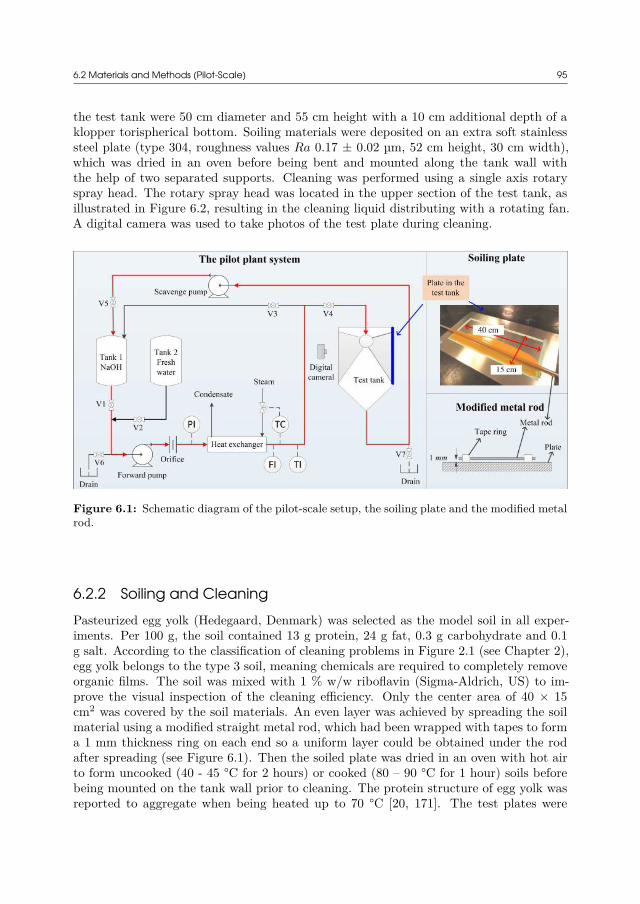
6.2 Materials and Methods (Pilot-Scale) 95
the test tank were 50 cm diameter and 55 cm height with a 10 cm additional depth of aklopper torispherical bottom. Soiling materials were deposited on an extra soft stainlesssteel plate (type 304, roughness values Ra 0.17 ± 0.02 µm, 52 cm height, 30 cm width),which was dried in an oven before being bent and mounted along the tank wall withthe help of two separated supports. Cleaning was performed using a single axis rotaryspray head. The rotary spray head was located in the upper section of the test tank, asillustrated in Figure 6.2, resulting in the cleaning liquid distributing with a rotating fan.A digital camera was used to take photos of the test plate during cleaning.
Figure 6.1: Schematic diagram of the pilot-scale setup, the soiling plate and the modified metalrod.
6.2.2 Soiling and CleaningPasteurized egg yolk (Hedegaard, Denmark) was selected as the model soil in all exper-iments. Per 100 g, the soil contained 13 g protein, 24 g fat, 0.3 g carbohydrate and 0.1g salt. According to the classification of cleaning problems in Figure 2.1 (see Chapter 2),egg yolk belongs to the type 3 soil, meaning chemicals are required to completely removeorganic films. The soil was mixed with 1 % w/w riboflavin (Sigma-Aldrich, US) to im-prove the visual inspection of the cleaning efficiency. Only the center area of 40 × 15cm2 was covered by the soil materials. An even layer was achieved by spreading the soilmaterial using a modified straight metal rod, which had been wrapped with tapes to forma 1 mm thickness ring on each end so a uniform layer could be obtained under the rodafter spreading (see Figure 6.1). Then the soiled plate was dried in an oven with hot airto form uncooked (40 - 45 °C for 2 hours) or cooked (80 – 90 °C for 1 hour) soils beforebeing mounted on the tank wall prior to cleaning. The protein structure of egg yolk wasreported to aggregate when being heated up to 70 °C [20, 171]. The test plates were
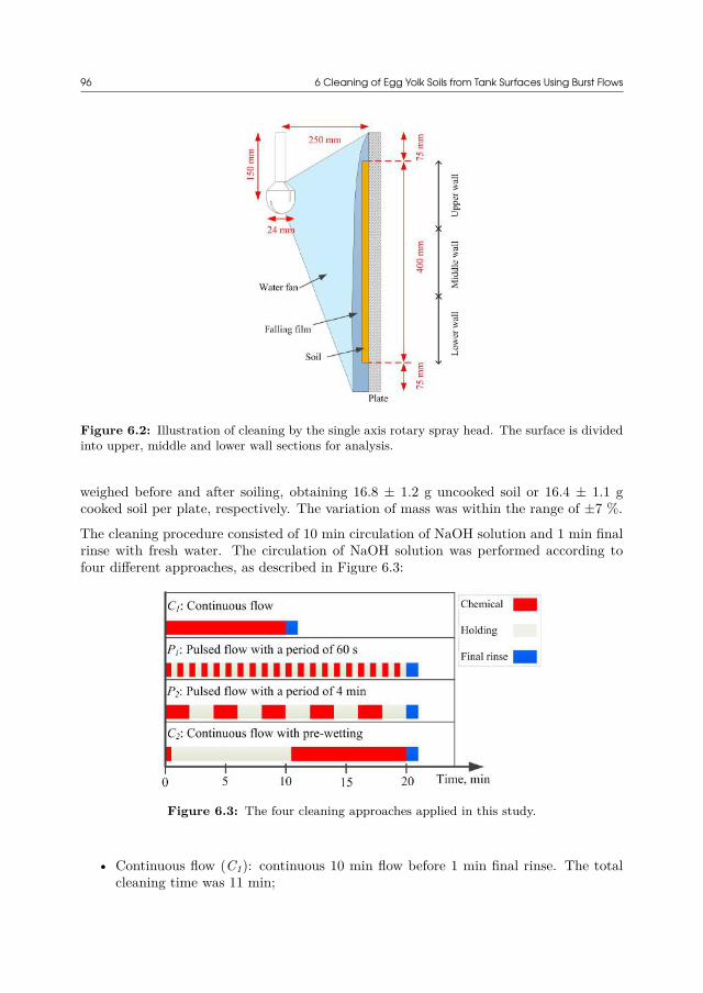
96 6 Cleaning of Egg Yolk Soils from Tank Surfaces Using Burst Flows
Figure 6.2: Illustration of cleaning by the single axis rotary spray head. The surface is dividedinto upper, middle and lower wall sections for analysis.
weighed before and after soiling, obtaining 16.8 ± 1.2 g uncooked soil or 16.4 ± 1.1 gcooked soil per plate, respectively. The variation of mass was within the range of ±7 %.
The cleaning procedure consisted of 10 min circulation of NaOH solution and 1 min finalrinse with fresh water. The circulation of NaOH solution was performed according tofour different approaches, as described in Figure 6.3:
Figure 6.3: The four cleaning approaches applied in this study.
• Continuous flow (C1): continuous 10 min flow before 1 min final rinse. The totalcleaning time was 11 min;
6.2 Materials and Methods (Pilot-Scale) 97
• Pulsed flow with a period of 60 s (P1): 30 s flow followed by 30 s break repeatedfor 20 times before the final rinse. The total cleaning time was 21 min;
• Pulsed flow with a period of 4 min (P2): 2 min flow followed by 2 min break repeatedfor 5 times prior to the final rinse, with a total cleaning time of 21 min;
• Continuous flow with pre-wetting (C2): 30 s flow followed by 10 min break and 9.5min continuous flow before the final rinse. The total cleaning time was 21 min.
The cleaning results were evaluated by taking photos of the test plate during each breakand after the final rinse. The first two approaches, C1 and P1, were mainly investigated.C2 and P2 were designed for comparison. The burst frequency of P2 was more similar tothe common industrial practices for tank cleaning operations. To reduce the damage tothe pumps as a result of frequent start-up and shut-down, the forward flow was controlledby alternatively opening or closing the butterfly valves V3 and V4, resulting in the switchbetween flow circulation (during breaks) and cleaning. The scavenge pump started whenthe liquid was accumulated at the test tank bottom above a certain level. The examinedparameters included temperature, flow rate and NaOH concentration, which are describedin Section 6.2.4. All experiments were performed at least in duplicates.
6.2.3 Determination of Soiling AreasThe remaining soiling areas were calculated with the help of the image analysis toolboxin Matlab (MathWorks, US). The normalized remaining soiling area y was defined as theratio of the remaining soiling area to the total initial soiling area, according to:
y = Remaining soiling area
Total soiling area before cleaning6.1
So y = 1 denotes completely dirty and y = 0 denotes completely clean. The soiled platewas equally divided into three sections (upper, middle and lower wall) with 13.33 cmheight for each (Figure 6.2). The different sections were analysed separately.
6.2.4 Factorial Experimental DesignAs shown in Table 6.1, the effects of temperature T , flow rate FR and NaOH concentrationC were evaluated in terms of the normalized remaining soiling area y. The experimentswere executed in a random order with the intention to randomize experimental errors[172]. A second-order regression model for the actual variables xi (indicating T , FR andC) was obtained by fitting the experimental results using Equation 6.2:
y = β0 +3∑
j=1βjxj +
3∑j=1
∑i<j
βijxixj + ϵ 6.2
where y is the predicted value of y. β0, βi and βij are the intercept, linear and interactionterms respectively and ϵ is the statistical error term. Adding one center point in thefactorial experimental design helped to examine the significance of curvature effects onthe model if a βiixi
2 term was added.

98 6 Cleaning of Egg Yolk Soils from Tank Surfaces Using Burst Flows
Table 6.1: 23 factorial experimental design indicating the coded and actual values of variables
RunsCoded levels of variables Actual levels of variables
Temp. Flow rate Conc. Temp. Flow rate Conc.X1 X2 X3 T , [°C] FR, [m3/h] C, [kg/m3]
Factorial points1 -1 -1 -1 25 0.9 12 1 -1 -1 55 0.9 13 -1 1 -1 25 1.5 14 1 1 -1 55 1.5 15 -1 -1 1 25 0.9 56 1 -1 1 55 0.9 57 -1 1 1 25 1.5 58 1 1 1 55 1.5 5
Center point9 0 0 0 40 1.2 3
6.2.5 Cost ModelThe total costs of cleaning by alkali solution (δT otal) were computed as the sum of thecosts of fresh water (δF resh water), chemical (δChemical), electricity by pumps (δElectricity)and sensible heat (δHeat). To calculate the cleaning costs that result in a certain amountof cleanliness, the following equation was used:
Cleaning costs
Degree of cleaning= δT otal
100 − 99 · y
= δF resh water + δChemical + δElectricity + δHeat
100 − 99 · y
6.3
where y is the corrected term of y by eliminating the unrealistic prediction errors as:
y =
0 y < 0y 0 ≤ y ≤ 11 y > 1
6.4
A degree of cleaning (DoC) value of 100 represents that all soils are removed (y = 0),and the value of 1 represents that no soil is removed (y = 1). The costs of fresh water,chemical, electricity and sensible heat were calculated through Equations 6.5 to 6.8 (re-written from Equations 3.2 to 3.5), noting the term t/3600 converted the time unit fromsecond to hour:
δF resh water = FR · t/3600 · φF resh water 6.5δChemical = FR · t/3600 · C · φChemical 6.6
δElectricity = (Pf + Ps) · t/3600 · φElectricity 6.7δHeat = FR · t/3600 · ρ · cP · (T − T0) · φHeat 6.8
6.3 Results and Discussion 99
where Pf and Ps are the powers of the forward and scavenge pumps, ρ (1,000 kg⁄m3) isthe density of water, cP (4,185.5 J⁄(kg °C)) is the heat capacity of water and T0 (25 °C) isroom temperature. The unit cost of each item was selected based on the prices in Danishindustries: φF resh water = 3.6 Euro⁄m3 including waste water treatment, φChemical = 1Euro⁄kg, φElectricity = 0.09 Euro⁄(kWh), φHeat = 2.6·10-8 Euro⁄J.
6.3 Results and Discussion
6.3.1 Cleaning DynamicsFigure 6.4 shows the normalized remaining soiling areas (of selected runs in Table 6.1,the results for all runs are provided in Appendix B) at different wall locations by usingcontinuous flow C1 and pulsed flow P1. Fewer soils remain in the upper wall sectionthan in the lower wall section at the same effective time, which is defined as the timewhen the liquid flow acts on the tank surface (actual cleaning time subtracted holdingtime). It means the fastest removal of deposit occurs in the upper part. As illustrated inFigure 6.2, the upper section is the closest to the rotary spray head and experiences thehighest impact force from the droplets in the liquid fan. However, thicker falling filmsform in the lower section as liquid flows down under gravity, implying higher wall shearstress in the lower section than in the upper section. The phenomena of (i) higher shearforce but slower cleaning rate in the lower wall section and (ii) lower shear force but fastercleaning rate in the upper wall section imply that the soil layers are mainly detached bythe direct impact of liquid droplets instead of falling films.
The results in Figure 6.4 reveal that pulsed flows are able to remove more deposits fromthe tank wall than continuous flows at the same effective time. There are two explanationsof the enhanced cleaning performance by pulsed flows: the increased holding time andthe improved shear force. The holding time between two bursts can provide additionaltime for the diffusion of the alkali solution into the soil outer layer and therefore improvesthe reaction rate. In between two bursts, the outer layer of soiling materials swells andbecomes weak, and is therefore more easily detached in the next burst [33]. For thecleaning by continuous flow, the impact force and falling film detach the outer swollenlayer constantly. But this process is restricted by the rate of diffusion and swelling, sothe mechanical force cannot remove as much soil as it can. However, for the cleaningby pulsed flow, the additional holding time between two pulses enables more soil layersto swell and thus removes more soil layers. The improved shear force is caused by theunstable falling film when stopping and starting a pulse. It is anticipated that a wavyfilm forms in the unsteady flow region. Consequently, the local maxima of wall shearstress, even local flow reversal, occur instantaneously at the front of the unstable freefalling film [86, 90]. Therefore, during the cleaning by pulsed flow, the unstable fallingfilm can contribute to the removal of soil materials by enhanced shear force. This effectis comparable to the pipe or filter cleaning operations where pulsed flows enhance localwall shear stress and hence improve the cleaning results [162, 168]. However, as discussedabove, cleaning by falling film is less significant than by the direct impact from the liquidfan. Therefore, the improved shear force due to pulsed flow can contribute to cleaning

100 6 Cleaning of Egg Yolk Soils from Tank Surfaces Using Burst Flows
Figure 6.4: Removal of uncooked soils for different conditions of temperature, flow rate andNaOH concentration, by using continuous flow without pre-wetting (C1) or pulsed flow of highfrequency (P1). Only the results of selected runs 1, 2, 3 and 5 in Table 6.1 are displayed. Theresults for all runs are displayed in Appendix B: (A) tank upper wall, (B) tank middle wall, (C)tank lower wall, (D) tank overall wall surface.
but is not the key factor.
The slopes in Figure 6.4 indicate the removal rate of uncooked egg yolk deposits by usingpulsed flow (P1). The cleaning dynamics by continuous flow (C1) could be analyzedthrough the discrete observations and are shown in Figure 6.5. Typical three-phasecleaning dynamics are revealed: the cleaning rate is initially slow due to the swelling ofsoil, then chunks are removed at a constant rate, and finally the removal is limited at thedecay phase. This profile is similar to the observations of Gillham et al. (2000) [162] andGoode et al. (2010) [42]. According to Figure 6.4, the most efficient cleaning occurs at lowalkali concentration, high temperature and high flow rate. Among the tested parameters,the alkali concentration and temperature contribute most to the swelling and removal of
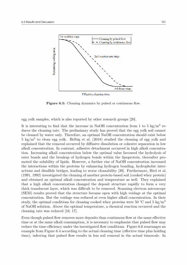
6.3 Results and Discussion 101
Figure 6.5: Cleaning dynamics by pulsed or continuous flow.
egg yolk samples, which is also reported by other research groups [20].
It is interesting to find that the increase in NaOH concentration from 1 to 5 kg/m3 re-duces the cleaning rate. The preliminary study has proved that the egg yolk soil cannotbe cleaned by water only. Therefore, an optimal NaOH concentration should exist below5 kg/m3 to clean egg yolk. Helbig et al. (2018) studied the cleaning of egg yolk andexplained that the removal occurred by diffusive dissolution or cohesive separation in lowalkali concentration. In contrast, adhesive detachment occurred in high alkali concentra-tion. Increasing alkali concentration below the optimal value favoured the hydrolysis ofester bonds and the breakup of hydrogen bonds within the lipoprotein, thereafter pro-moted the solubility of lipids. However, a further rise of NaOH concentration increasedthe interactions within the proteins by enhancing hydrogen bonding, hydrophobic inter-actions and disulfide bridges, leading to worse cleanability [39]. Furthermore, Bird et al.(1991, 1992) investigated the cleaning of another protein-based soil (cooked whey protein)and obtained an optimal alkali concentration and temperature as well. They explainedthat a high alkali concentration changed the deposit structure rapidly to form a verythick translucent layer, which was difficult to be removed. Scanning electron microscope(SEM) results proved that the structure became open with high voidage at the optimalconcentration. But the voidage was reduced at even higher alkali concentration. In theirstudy, the optimal conditions for cleaning cooked whey proteins were 50 °C and 5 kg/m3
of NaOH solution. Above the optimal temperature, a chemical reaction occurred and thecleaning rate was reduced [16, 17].
Even though pulsed flow removes more deposits than continuous flow at the same effectivetime or at the same alkali consumption, it is necessary to emphasize that pulsed flow mayreduce the time efficiency under the investigated flow conditions. Figure 6.6 rearranges anexample from Figure 6.4 according to the actual cleaning time (effective time plus holdingtime), inferring that pulsed flow results in less soil removal in the actual timescale. In
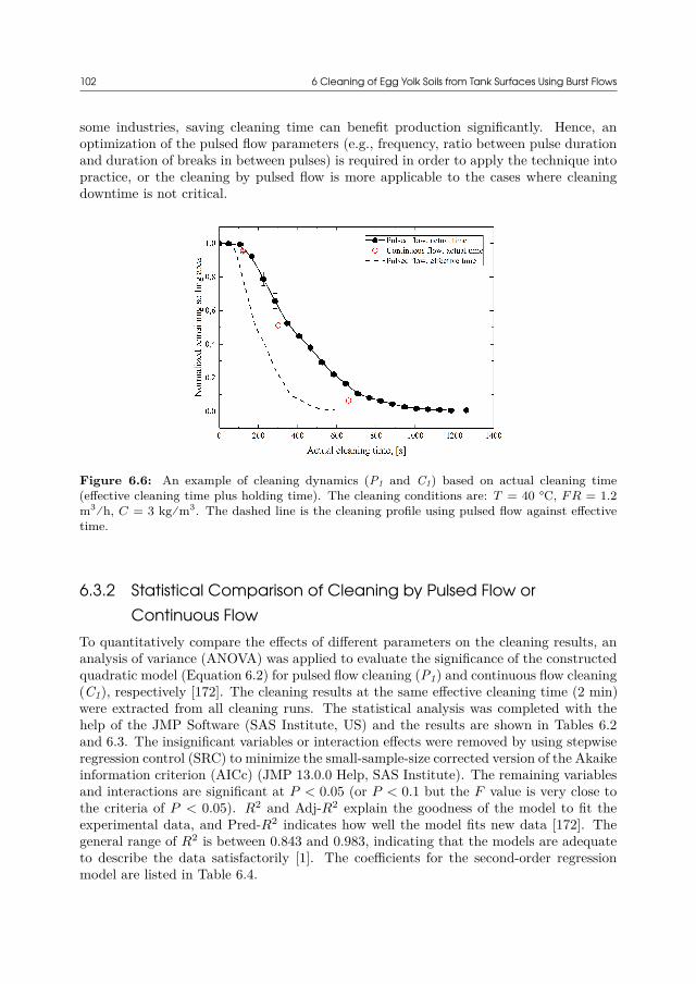
102 6 Cleaning of Egg Yolk Soils from Tank Surfaces Using Burst Flows
some industries, saving cleaning time can benefit production significantly. Hence, anoptimization of the pulsed flow parameters (e.g., frequency, ratio between pulse durationand duration of breaks in between pulses) is required in order to apply the technique intopractice, or the cleaning by pulsed flow is more applicable to the cases where cleaningdowntime is not critical.
Figure 6.6: An example of cleaning dynamics (P1 and C1) based on actual cleaning time(effective cleaning time plus holding time). The cleaning conditions are: T = 40 °C, F R = 1.2m3⁄h, C = 3 kg⁄m3. The dashed line is the cleaning profile using pulsed flow against effectivetime.
6.3.2 Statistical Comparison of Cleaning by Pulsed Flow orContinuous Flow
To quantitatively compare the effects of different parameters on the cleaning results, ananalysis of variance (ANOVA) was applied to evaluate the significance of the constructedquadratic model (Equation 6.2) for pulsed flow cleaning (P1) and continuous flow cleaning(C1), respectively [172]. The cleaning results at the same effective cleaning time (2 min)were extracted from all cleaning runs. The statistical analysis was completed with thehelp of the JMP Software (SAS Institute, US) and the results are shown in Tables 6.2and 6.3. The insignificant variables or interaction effects were removed by using stepwiseregression control (SRC) to minimize the small-sample-size corrected version of the Akaikeinformation criterion (AICc) (JMP 13.0.0 Help, SAS Institute). The remaining variablesand interactions are significant at P < 0.05 (or P < 0.1 but the F value is very close tothe criteria of P < 0.05). R2 and Adj-R2 explain the goodness of the model to fit theexperimental data, and Pred-R2 indicates how well the model fits new data [172]. Thegeneral range of R2 is between 0.843 and 0.983, indicating that the models are adequateto describe the data satisfactorily [1]. The coefficients for the second-order regressionmodel are listed in Table 6.4.

6.3 Results and Discussion 103
Table 6.2: Analysis for the cleaning of uncooked soil by using pulsed flow (P1) at 2 min ofeffective time.
Source ofvariance
Upper wall Middle wall Lower wall Overall wallDFa F DFa F DFa F DFa F
Model 5 44.62c 5 52.19c 5 29.39c 5 136.18c
X1 1 13.40c 1 21.72c 1 28.15c 1 81.86c
X2 1 7.65d 1 26.32c 1 11.19c 1 44.21c
X3 1 183.85c 1 148.92c 1 74.35c 1 442.82c
X1X2 SRCb SRCb SRCb SRCb
X1X3 1 13.49c 1 33.79c 1 24.18c 1 79.30c
X2X3 1 4.72e 1 20.21c 1 9.06d 1 32.69c
Residual 12 12 12 12Lack of fit 3 2.30 3 0.83 3 6.71d 3 3.34Pure error 9 9 9 9
Total model 17 17 17 17R2 0.949 0.956 0.924 0.983
Adj-R2 0.928 0.938 0.893 0.975Pred-R2 0.865 0.917 0.849 0.968
a DF: Degree of freedomb SRC: Removed by “stepwise regression control” modelc P ≤ 0.01d P ≤ 0.05e P ≤ 0.1
The results in Tables 6.2 and 6.3 show the effects of the investigated parameters on thecleaning behavior, and can be summarized as follows:
• For both cleaning approaches (continuous C1 and pulsed P1), the most importantparameter of the cleaning process is the alkali concentration (X3). Furthermore,the main effects of temperature (X1) and flow rate (X2) as well as the interac-tions between temperature and alkali concentration (X1X3) and between flow rateand alkali concentration (X2X3) are significant as well. The interaction betweentemperature and flow rate (X1X2) can, however, be eliminated.
• For pulsed flow cleaning, the effects of temperature and its interaction with alkaliconcentration are greater than the effects of flow rate and its interaction with alkaliconcentration. In contrast, the opposite is true for continuous flow cleaning.
• The quadratic curvature in the response model, implied by the lack-of-fit statistic, isinsignificant or less significant compared with the other main factors or interactions.However, the current experimental design with only one replicated center pointcannot identify which of the three variables exhibit curvature. An alternative designis to augment the 23 design with more axial runs, called a central composite design[1, 172]. Nonetheless, this study keeps the proposed design and model, because thecurvature effect is less significant than the others in the studied ranges of conditions.
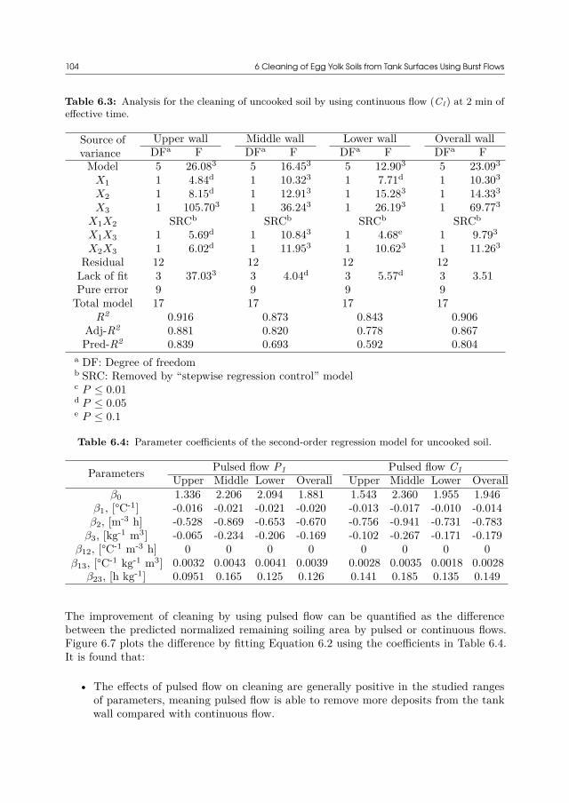
104 6 Cleaning of Egg Yolk Soils from Tank Surfaces Using Burst Flows
Table 6.3: Analysis for the cleaning of uncooked soil by using continuous flow (C1) at 2 min ofeffective time.
Source ofvariance
Upper wall Middle wall Lower wall Overall wallDFa F DFa F DFa F DFa F
Model 5 26.083 5 16.453 5 12.903 5 23.093
X1 1 4.84d 1 10.323 1 7.71d 1 10.303
X2 1 8.15d 1 12.913 1 15.283 1 14.333
X3 1 105.703 1 36.243 1 26.193 1 69.773
X1X2 SRCb SRCb SRCb SRCb
X1X3 1 5.69d 1 10.843 1 4.68e 1 9.793
X2X3 1 6.02d 1 11.953 1 10.623 1 11.263
Residual 12 12 12 12Lack of fit 3 37.033 3 4.04d 3 5.57d 3 3.51Pure error 9 9 9 9
Total model 17 17 17 17R2 0.916 0.873 0.843 0.906
Adj-R2 0.881 0.820 0.778 0.867Pred-R2 0.839 0.693 0.592 0.804
a DF: Degree of freedomb SRC: Removed by “stepwise regression control” modelc P ≤ 0.01d P ≤ 0.05e P ≤ 0.1
Table 6.4: Parameter coefficients of the second-order regression model for uncooked soil.
Parameters Pulsed flow P1 Pulsed flow C1Upper Middle Lower Overall Upper Middle Lower Overall
β0 1.336 2.206 2.094 1.881 1.543 2.360 1.955 1.946β1, [°C-1] -0.016 -0.021 -0.021 -0.020 -0.013 -0.017 -0.010 -0.014
β2, [m-3 h] -0.528 -0.869 -0.653 -0.670 -0.756 -0.941 -0.731 -0.783β3, [kg-1 m3] -0.065 -0.234 -0.206 -0.169 -0.102 -0.267 -0.171 -0.179
β12, [°C-1 m-3 h] 0 0 0 0 0 0 0 0β13, [°C-1 kg-1 m3] 0.0032 0.0043 0.0041 0.0039 0.0028 0.0035 0.0018 0.0028
β23, [h kg-1] 0.0951 0.165 0.125 0.126 0.141 0.185 0.135 0.149
The improvement of cleaning by using pulsed flow can be quantified as the differencebetween the predicted normalized remaining soiling area by pulsed or continuous flows.Figure 6.7 plots the difference by fitting Equation 6.2 using the coefficients in Table 6.4.It is found that:
• The effects of pulsed flow on cleaning are generally positive in the studied rangesof parameters, meaning pulsed flow is able to remove more deposits from the tankwall compared with continuous flow.
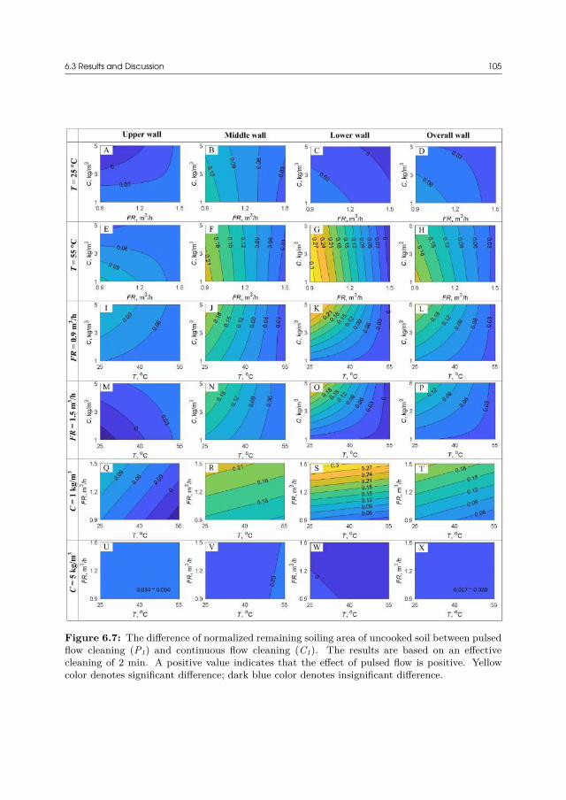
6.3 Results and Discussion 105
Figure 6.7: The difference of normalized remaining soiling area of uncooked soil between pulsedflow cleaning (P1) and continuous flow cleaning (C1). The results are based on an effectivecleaning of 2 min. A positive value indicates that the effect of pulsed flow is positive. Yellowcolor denotes significant difference; dark blue color denotes insignificant difference.
106 6 Cleaning of Egg Yolk Soils from Tank Surfaces Using Burst Flows
• The difference between pulsed flow and continuous flow is more significant at hightemperature and at low alkali concentration. The variation of the flow rate doesnot make a large difference between the two cleaning methods. This is becausetemperature and the alkali concentration are key factors contributing to reactions,which is in line with the idea of pulsed flow cleaning that allows a longer reactiontime. Higher flow rates lead to greater mechanical impact, which, however, is notthe limiting factor in this study because the applied flow rate is high enough todetach the swollen soils.
• The difference between the two cleaning approaches is less substantial at the upperwall section than at the lower wall section. The distance from the rotary sprayhead to the tank surface increases from the tank top to the bottom. Hence, themechanical forces exhibited on the wall decline from the upper section to the lowersection. As discussed above, the improvement of cleaning by pulsed flow is lessaffected by this impact. Therefore, the enhancement of cleaning by pulsed flowbecomes less apparent at the upper wall section.
• For the lower wall section or the overall wall, the greatest improvement by usingpulsed flow occurs at high temperature and low flow rate, or low alkali concentra-tion and high flow rate. At low temperature and high alkali concentration, thecontribution of pulsation is small.
6.3.3 Cleaning of Uncooked Soils with Different Pulsed or ContinuousApproaches
Figure 6.8 compares the cleaning of uncooked soil deposits with different pulsed andcontinuous approaches. After the final rinse, the improvement of cleaning using pulsedflows is observed but not obvious in the upper and middle wall sections when comparedwith continuous flows. The reason is that only the pictures after final rinse were taken inthe cleaning experiments by continuous flows, when most soil deposits have been removed.It has been indicated in Figure 6.5 that the improvement by pulsed flow is the mostsignificant at the stage when chunks of deposits are removed at a constant rate (normally150 - 500 s effective time for the upper and middle wall sections). Therefore, it is a logicaldeduction that a more clear difference between the pulsed and continuous approaches canbe observed at some latent time points during alkali circulation. In Figure 6.8C, pulsedflow can remove ca. 15% more soils than continuous flow at the lower wall section. Itconfirms the hypothesis that a clear difference occurs before the cleaning approaches theend, as the cleaning of the lower wall section still lies in the constant-rate stage (illustratedin Figure 6.5) after final rinse.
Pulsed flow with a lower frequency (P2) is less effective than that with a higher frequency(P1) at the upper wall section, middle wall section and the overall surface. The repeatedbursts of liquid contribute to the removal of the swollen soil layers instantly by mechanicalforces, exposing the hard layers to fresh liquid in the next burst. However, the low impactforces at the lower wall section restrict the removal of the outer layer of soil [102], therebythe influence of pulse frequency is not significant. The resulted best cleaning performance
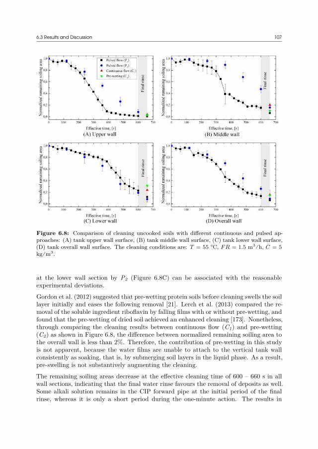
6.3 Results and Discussion 107
Figure 6.8: Comparison of cleaning uncooked soils with different continuous and pulsed ap-proaches: (A) tank upper wall surface, (B) tank middle wall surface, (C) tank lower wall surface,(D) tank overall wall surface. The cleaning conditions are: T = 55 °C, F R = 1.5 m3⁄h, C = 5kg⁄m3.
at the lower wall section by P2 (Figure 6.8C) can be associated with the reasonableexperimental deviations.
Gordon et al. (2012) suggested that pre-wetting protein soils before cleaning swells the soillayer initially and eases the following removal [21]. Lerch et al. (2013) compared the re-moval of the soluble ingredient riboflavin by falling films with or without pre-wetting, andfound that the pre-wetting of dried soil achieved an enhanced cleaning [173]. Nonetheless,through comparing the cleaning results between continuous flow (C1) and pre-wetting(C2) as shown in Figure 6.8, the difference between normalized remaining soiling area tothe overall wall is less than 2%. Therefore, the contribution of pre-wetting in this studyis not apparent, because the water films are unable to attach to the vertical tank wallconsistently as soaking, that is, by submerging soil layers in the liquid phase. As a result,pre-swelling is not substantively augmenting the cleaning.
The remaining soiling areas decrease at the effective cleaning time of 600 – 660 s in allwall sections, indicating that the final water rinse favours the removal of deposits as well.Some alkali solution remains in the CIP forward pipe at the initial period of the finalrinse, whereas it is only a short period during the one-minute action. The results in
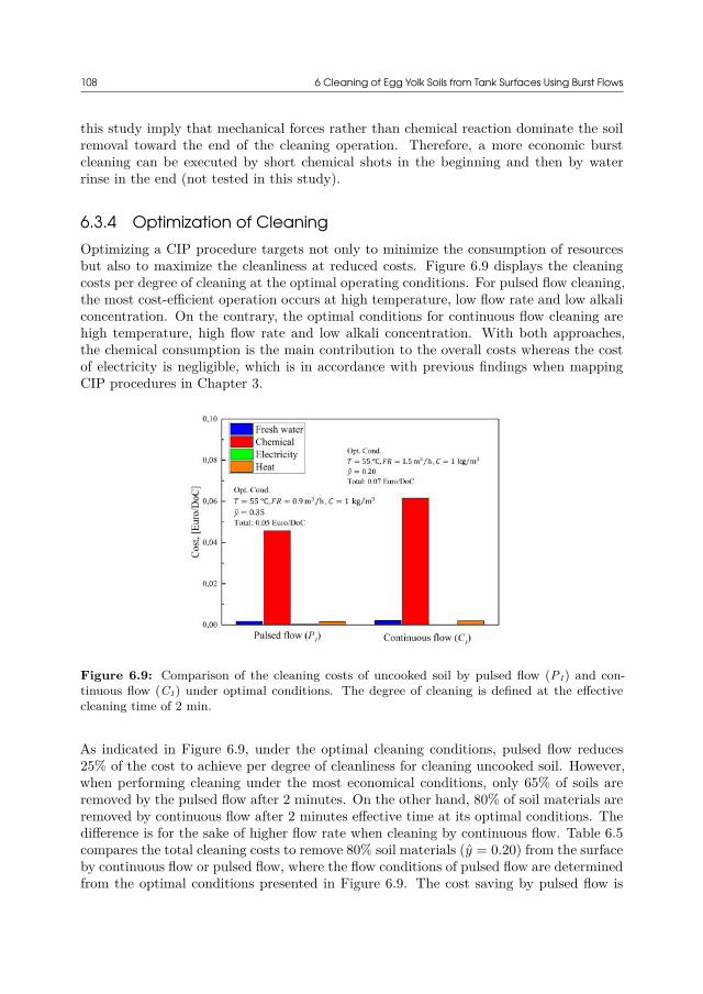
108 6 Cleaning of Egg Yolk Soils from Tank Surfaces Using Burst Flows
this study imply that mechanical forces rather than chemical reaction dominate the soilremoval toward the end of the cleaning operation. Therefore, a more economic burstcleaning can be executed by short chemical shots in the beginning and then by waterrinse in the end (not tested in this study).
6.3.4 Optimization of CleaningOptimizing a CIP procedure targets not only to minimize the consumption of resourcesbut also to maximize the cleanliness at reduced costs. Figure 6.9 displays the cleaningcosts per degree of cleaning at the optimal operating conditions. For pulsed flow cleaning,the most cost-efficient operation occurs at high temperature, low flow rate and low alkaliconcentration. On the contrary, the optimal conditions for continuous flow cleaning arehigh temperature, high flow rate and low alkali concentration. With both approaches,the chemical consumption is the main contribution to the overall costs whereas the costof electricity is negligible, which is in accordance with previous findings when mappingCIP procedures in Chapter 3.
Figure 6.9: Comparison of the cleaning costs of uncooked soil by pulsed flow (P1) and con-tinuous flow (C1) under optimal conditions. The degree of cleaning is defined at the effectivecleaning time of 2 min.
As indicated in Figure 6.9, under the optimal cleaning conditions, pulsed flow reduces25% of the cost to achieve per degree of cleanliness for cleaning uncooked soil. However,when performing cleaning under the most economical conditions, only 65% of soils areremoved by the pulsed flow after 2 minutes. On the other hand, 80% of soil materials areremoved by continuous flow after 2 minutes effective time at its optimal conditions. Thedifference is for the sake of higher flow rate when cleaning by continuous flow. Table 6.5compares the total cleaning costs to remove 80% soil materials (y = 0.20) from the surfaceby continuous flow or pulsed flow, where the flow conditions of pulsed flow are determinedfrom the optimal conditions presented in Figure 6.9. The cost saving by pulsed flow is
6.3 Results and Discussion 109
21 - 31% compared to the cleaning by continuous flow. The generation of waste wateris also lower when cleaning by pulsed flows. However, an increase in downtime shouldbe considered when implementing burst cleaning in practice, as previously reported inFigure 6.6. It can still be concluded that tank cleaning by using pulsed flow makes theper unit consumption of cleaning detergent more valuable.
Table 6.5: Analysis for the cleaning of uncooked soil (y = 0.20) by using continuous flow (C1)at 2 min of effective time
Parameters Continuous flow C1 Pulsed flow P1T , [°C] 55 55 55
FR, [m3 h] 1.5 1.5 0.9C, [kg m-3] 1 1 1
Effective cleaning timea, [s] 120 95 138Actual cleaning timea, [s] 120 185 258
Waste water volumeb, [m3] 0.050 0.040 0.035Total cost, [10-2 Euro/DoC] 6.6 5.2 4.6
Cost saving - 21% 31%a Effective cleaning time denotes the circulation time of alkali solution. Actual cleaning
time is the sum of effective cleaning time and holding time.b Alkaline solutions are circulated in experiments. Waste water volume is calculated
as the product of flow rate and effective cleaning time, assuming chemical solutionsare used without recycle.
6.3.5 Cleaning of Cooked Soils with Different ApproachesFigure 6.10 shows the cleaning results of cooked soils with different continuous and pulsedapproaches. Larger soiling areas are obtained in all observations compared with thecleaning of uncooked soils at the same flow conditions (see Figure 6.8). The difference iscaused by the nature of deposits that can strongly affect the cleaning behavior. Heatingprotein-based soil over its denaturation temperature makes the material harder to remove[21]. Some results of cleaning cooked soils are consistent with the results of cleaninguncooked soils: pulsed flow improves cleaning compared with continuous flow; higherpulse frequency favours the removal of deposits at the upper wall section compared tolower pulse frequency; the final rinse with water can detach the swollen soil when thecleaning tends to finish.
On the other hand, the influence of pulsed flows becomes more noticeable during the clean-ing of cooked soil compared with the cleaning of uncooked soil. Taking the continuousflow cleaning C1 as contrast, the cleanings performed by pulsed flow with low frequency(P2) and pulsed flow with high frequency (P1) can respectively improve the removal ofdeposits by 33.0% and 51.1% of the overall surface. However, the negative improvementby pre-wetting to the middle wall section can be associated with experimental deviations,as displayed in Figure 6.10B.
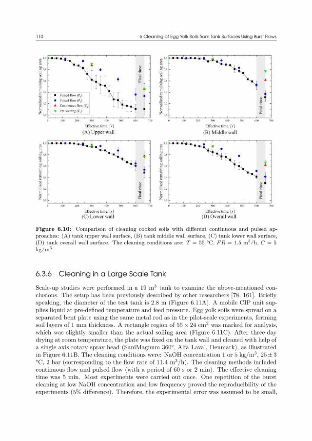
110 6 Cleaning of Egg Yolk Soils from Tank Surfaces Using Burst Flows
Figure 6.10: Comparison of cleaning cooked soils with different continuous and pulsed ap-proaches: (A) tank upper wall surface, (B) tank middle wall surface, (C) tank lower wall surface,(D) tank overall wall surface. The cleaning conditions are: T = 55 °C, F R = 1.5 m3⁄h, C = 5kg⁄m3.
6.3.6 Cleaning in a Large Scale Tank
Scale-up studies were performed in a 19 m3 tank to examine the above-mentioned con-clusions. The setup has been previously described by other researchers [78, 161]. Brieflyspeaking, the diameter of the test tank is 2.8 m (Figure 6.11A). A mobile CIP unit sup-plies liquid at pre-defined temperature and feed pressure. Egg yolk soils were spread on aseparated bent plate using the same metal rod as in the pilot-scale experiments, formingsoil layers of 1 mm thickness. A rectangle region of 55 × 24 cm2 was marked for analysis,which was slightly smaller than the actual soiling area (Figure 6.11C). After three-daydrying at room temperature, the plate was fixed on the tank wall and cleaned with help ofa single axis rotary spray head (SaniMagnum 360°, Alfa Laval, Denmark), as illustratedin Figure 6.11B. The cleaning conditions were: NaOH concentration 1 or 5 kg/m3, 25 ± 3°C, 2 bar (corresponding to the flow rate of 11.4 m3/h). The cleaning methods includedcontinuous flow and pulsed flow (with a period of 60 s or 2 min). The effective cleaningtime was 5 min. Most experiments were carried out once. One repetition of the burstcleaning at low NaOH concentration and low frequency proved the reproducibility of theexperiments (5% difference). Therefore, the experimental error was assumed to be small,
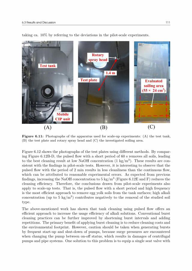
6.3 Results and Discussion 111
taking ca. 10% by referring to the deviations in the pilot-scale experiments.
Figure 6.11: Photographs of the apparatus used for scale-up experiments: (A) the test tank,(B) the test plate and rotary spray head and (C) the investigated soiling area.
Figure 6.12 shows the photographs of the test plates using different methods. By compar-ing Figure 6.12B-D, the pulsed flow with a short period of 60 s removes all soils, leadingto the best cleaning result at low NaOH concentration (1 kg/m3). These results are con-sistent with the findings in pilot-scale tests. However, it is interesting to observe that thepulsed flow with the period of 2 min results in less cleanliness than the continuous flow,which can be attributed to reasonable experimental errors. As expected from previousfindings, increasing the NaOH concentration to 5 kg/m3 (Figure 6.12E and F) reduces thecleaning efficiency. Therefore, the conclusions drawn from pilot-scale experiments alsoapply to scale-up tests. That is, the pulsed flow with a short period and high frequencyis the most efficient approach to remove egg yolk soils from the tank surfaces; high alkaliconcentration (up to 5 kg/m3) contributes negatively to the removal of the studied soiltype.
The above-mentioned work has shown that tank cleaning using pulsed flow offers anefficient approach to increase the usage efficiency of alkali solutions. Conventional burstcleaning practices can be further improved by shortening burst intervals and addingrepetitions. The primary benefit of applying burst cleaning is to reduce cleaning costs andthe environmental footprint. However, caution should be taken when generating burstsby frequent start-up and shut-down of pumps, because surge pressures are encounteredwhen changing the pump between on-off status, which results in damages of centrifugalpumps and pipe systems. One solution to this problem is to equip a single seat valve with
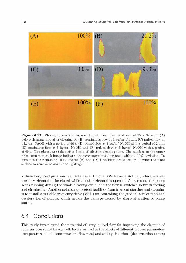
112 6 Cleaning of Egg Yolk Soils from Tank Surfaces Using Burst Flows
Figure 6.12: Photographs of the large scale test plate (evaluated area of 55 × 24 cm2) (A)before cleaning, and after cleaning by (B) continuous flow at 1 kg/m3 NaOH, (C) pulsed flow at1 kg/m3 NaOH with a period of 60 s, (D) pulsed flow at 1 kg/m3 NaOH with a period of 2 min,(E) continuous flow at 5 kg/m3 NaOH, and (F) pulsed flow at 5 kg/m3 NaOH with a periodof 60 s. The photos are taken after 5 min of effective cleaning time. The number on the upperright corners of each image indicates the percentage of soiling area, with ca. 10% deviation. Tohighlight the remaining soils, images (B) and (D) have been processed by blurring the platesurface to remove noises due to lighting.
a three body configuration (i.e. Alfa Laval Unique SSV Reverse Acting), which enablesone flow channel to be closed while another channel is opened. As a result, the pumpkeeps running during the whole cleaning cycle, and the flow is switched between feedingand circulating. Another solution to protect facilities from frequent starting and stoppingis to install a variable frequency drive (VFD) for controlling the gradual acceleration anddeceleration of pumps, which avoids the damage caused by sharp alteration of pumpstatus.
6.4 ConclusionsThis study investigated the potential of using pulsed flow for improving the cleaning oftank surfaces soiled by egg yolk layers, as well as the effects of different process parameters(temperature, alkali concentration, flow rate) and soiling situations (denaturation or not)

6.4 Conclusions 113
on the cleaning results. The primary investigation was performed at pilot-scale, and themain findings were then examined in scale-up tests.
In the pilot-scale tests, the optimal conditions to remove egg yolk were low alkali con-centration, high temperature and high flow rate. The interactions of alkali concentrationwith the other parameters affected the cleaning of the protein- and lipid-based soilingmaterial as well. For a given effective circulation time of alkali solution, the remainingsoiling areas, cleaned with continuous or pulsed flows, could be expressed using a second-order regression model. Pulsed flow with a high frequency resulted in more removal ofsoil deposits than that with a low pulsing frequency. The enhancement of cleaning bypulsed flow occurs primarily because the additional holding time is provided for soil lay-ers to react and swell, which has the benefit that the materials become easy to removein the next pulse of flow. Pre-wetting prior to continuous flow operation insignificantlyimproved the cleaning result. It was found that cooked soil material heated above itsdenaturation temperature made the soil more difficult to detach. However, the enhancedcleaning behavior by pulsed flow became more obvious when removing cooked soils.
The main findings at pilot-scale were also found in full scale tests. It was verified thatthe cleaning efficiency was highly improved by the pulsed flow with short period andhigh frequency. The negative contribution of high alkali concentration (5 kg/m3) wasstill observed after scale-up. As a result, this work provided a quantitative measure todemonstrate that pulsed flow improves tank cleaning results by reducing the relativeconsumption of cleaning detergent in order to achieve a certain cleanliness.
List of Nomenclature in Chapter 6The following nomenclature is only valid for this chapter. Some symbols are used in otherchapters but with different meanings. Otherwise, the symbols are specifically explainedin the text if there is no nomenclature in some chapter.
Roman LetterscP Heat capacity of water, [J kg-1 °C-1]C Alkali concentration, [kg m-3]F F -value in ANOVAFR Flow rate, [m3 h-1]P P -value in hypothesis testingPf Power of forward pump, [kW]Ps Power of scavenge pump, [kW]T Temperature, [°C]T0 Room temperature, [°C]xi Actual variable iXi Coded variable iy Normalized remaining soiling areay Predicted value of yy Corrected term of y

114 6 Cleaning of Egg Yolk Soils from Tank Surfaces Using Burst Flows
Greek Lettersβ0, βi, βij Coefficients in the second-order regression modelδi Cleaning cost of item iϵ Statistical errorρ Density, [kg m-3]φi Unit cost of item i
CHAPTER7A Three-Stage
Measurement-BasedCIP System for
Reducing WaterConsumption
7.1 Introduction
In CIP operations, the terms recycling and recovery are to a certain extent identical,meaning that the cleaning liquid is reused more than once. Figure 7.1 illustrates threecommon CIP systems. For a single-use CIP system, the cleaning medium needs to beprepared freshly, and sent directly to drain after passing through the equipment andpiping being cleaned. It reduces the possibility of cross-contamination and potentialspore formation. However, it is expensive to operate. A partial recovery system recoversthe detergent solution in the recovery tank for use in the next detergent or pre-rinse step.A full recovery system returns the cleaning fluid back to the supply tank [110]. Recoverysystems are commonly applied in food industries because of lower energy requirement,lower water consumption and reduced chemical losses. Single-use CIP is normally seenwhere a high level of hygiene is required, like in the pharmaceutical industry [6].
Current CIP monitoring systems normally consist of conductivity probes, flow metersand temperature probes, etc., with the purpose to ensure that the system is under a stateof control. The cleaning procedure is usually defined based on time, which means thatthe cleaning cycle starts when both temperature and conductivity measurements reachthe critical points, and ends after a pre-defined period. If a recovery process is applied,the recovery starts when the conductivity output at the return flow reaches a set pointor after the detergent has been added for a specific period [6]. However, a time-basedCIP recipe generally consumes more resources than needed, because the allocated time
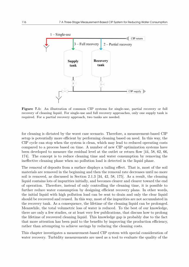
116 7 A Three-Stage Measurement-Based CIP System for Reducing Water Consumption
Figure 7.1: An illustration of common CIP systems for single-use, partial recovery or fullrecovery of cleaning liquid. For single-use and full recovery approaches, only one supply tank isrequired. For a partial recovery approach, two tanks are needed.
for cleaning is dictated by the worst case scenario. Therefore, a measurement-based CIPsetup is potentially more efficient by performing cleaning based on need. In this way, theCIP cycle can stop when the system is clean, which may lead to reduced operating costscompared to a process based on time. A number of new CIP optimization systems havebeen developed to measure the residual level at the outlet or return flow [44, 58, 62, 66,174]. The concept is to reduce cleaning time and water consumption by removing theineffective cleaning phase when no pollution load is detected in the liquid phase.
The removal of deposits from a surface displays a tailing effect. That is, most of the soilmaterials are removed in the beginning and then the removal rate decreases until no moresoil is removed, as discussed in Section 2.1.3 [34, 42, 58, 175]. As a result, the cleaningliquid contains lots of impurities initially, and becomes clearer and clearer toward the endof operation. Therefore, instead of only controlling the cleaning time, it is possible tofurther reduce water consumption by designing efficient recovery plans. In other words,the initial liquid with high pollution load can be sent to drain and only the clear liquidshould be recovered and reused. In this way, most of the impurities are not accumulated inthe recovery tank. As a consequence, the lifetime of the cleaning liquid can be prolonged.Meanwhile, the total volumetric loss of water is reduced. To the best of our knowledge,there are only a few studies, or at least very few publications, that discuss how to prolongthe lifetime of recovered cleaning liquid. This knowledge gap is probably due to the factthat more attention has been paid to the benefits by improving the production efficiency,rather than attempting to achieve savings by reducing the cleaning costs.
This chapter investigates a measurement-based CIP system with special consideration ofwater recovery. Turbidity measurements are used as a tool to evaluate the quality of the
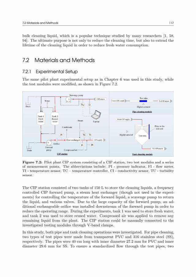
7.2 Materials and Methods 117
bulk cleaning liquid, which is a popular technique studied by many researchers [1, 58,94]. The ultimate purpose is not only to reduce the cleaning time, but also to extend thelifetime of the cleaning liquid in order to reduce fresh water consumption.
7.2 Materials and Methods
7.2.1 Experimental SetupThe same pilot plant experimental setup as in Chapter 6 was used in this study, whilethe test modules were modified, as shown in Figure 7.2.
Figure 7.2: Pilot plant CIP system consisting of a CIP station, two test modules and a seriesof measurement points. The abbreviations include: PI - pressure indicator, FI - flow meter,TI - temperature sensor, TC – temperature controller, CI - conductivity sensor, TU - turbiditysensor.
The CIP station consisted of two tanks of 150 L to store the cleaning liquids, a frequencycontrolled CIP forward pump, a steam heat exchanger (though not used in the experi-ments) for controlling the temperature of the forward liquid, a scavenge pump to returnthe liquid, and various valves. Due to the large capacity of the forward pump, an ad-ditional exchangeable orifice was installed downstream of the forward pump in order toreduce the operating range. During the experiments, tank 1 was used to store fresh water,and tank 2 was used to store reused water. Compressed air was applied to remove anyremaining liquid from the plant. The CIP station could be manually connected to theinvestigated testing modules through V-band clamps.
In this study, both pipe and tank cleaning operations were investigated. For pipe cleaning,two types of test pipes were made from transparent PVC and 316 stainless steel (SS),respectively. The pipes were 40 cm long with inner diameter 27.2 mm for PVC and innerdiameter 29.6 mm for SS. To ensure a standardized flow through the test pipes, two
118 7 A Three-Stage Measurement-Based CIP System for Reducing Water Consumption
straight pipes of 1 m and 0.4 m length were inserted before and after the test section,respectively, which were larger than the requirement of a five-time-diameter length tostabilize flows [176]. After cleaning, the liquid was directed to the reuse tank or to drainbypassing the scavenge pump. For tank cleaning, the test tank (50 cm diameter, 55 cmheight + 10 cm additional depth of a klopper torispherical bottom) surface was madefrom transparent PVC. To quantify and spread soils uniformly, two types of removabletest plates were made from soft PVC and 304 stainless steel (50 cm height, 30 cm width).The SS plates were bend to the same radius as the tank wall. After soiling, the plates werefixed along the tank wall by two separated supports. The tank cleaning was performedwith the help of a rotary spray head (the same as Figure 6.2). After cleaning, the liquidwas led to the reuse water tank or to drain by the scavenge pump. A digital camera wasused to record the tank cleaning and PVC pipe cleaning operations.
Apart from the steam valve, all valves were manually actuated. The CIP setup comprisedtwo pressure indicators (PI), a flow meter (FI), temperature sensors (TI) and in additionto a controller (TC) for adjusting the steam flow to the heat exchanger. A conductiv-ity sensor (CI, TetraCon 325, WTW, Weilheim, Germany) and a turbidity sensor (TU,STS01, Seli GmbH, Neuenkirchen, Germany) were installed at the outlet of the testingmodules (ca. 50 cm away from the pipe module or ca. 1 m away from the tank bottom)and the data could be logged to a laptop for analysis.
7.2.2 Soiling
Mustard (First Price “staerk sennep”) was used as model soil in all experiments. Theingredients were 48% water, 29% vinegar, 18% ground mustard seeds and 3% others. Per100 g, the soil contained 4.8 g fat, 4.8 g protein, 3.5 g carbohydrate and 3.1 g salt. Tosoil the pipes, mustard was filled into the pipe. The two ends of the pipe were closedby two plastic caps. Then the filled pipe was weighed (w1) and put immediately to thetesting module after removing the caps. The two caps were weighed again (w2), as somemustard stuck to the caps. The amount of mustard in the pipe was calculated as:
wsoil = w1 − w2 − w0 7.1
where w0 is the weight of the dry pipe. The average mass of soils was 246.3 ± 3.3 g inthe PVC pipe and 292.0 ± 13.1 g in the SS pipe.
To soil the plates, mustard was squeezed on the plate and spread out as smooth as possibleusing a glass wiper cleaning brush. The plate was only soiled from 5 to 45 cm heightof the plate, because the top and bottom parts needed to be attached to the supportsto be mounted on the tank wall. The mass of mustard was calculated as the differencebetween the weight of the plate before and after soiling, to be 115.1±3.7 g, correspondingto 0.096 ± 0.003 g soil/cm2 surface. The plate was left at room temperature for 3 hours.Then the plate was fixed to the tank wall for cleaning with the help of the supports.
7.2 Materials and Methods 119
7.2.3 MeasurementsThe cleanliness of cleaning water was measured by turbidity. The mustard residues onthe surfaces could be visually observed or by analysing the recorded pictures. In addition,a swab-click-read method was applied to indicate whether protein residuals remained onthe surface, which was performed according to the instruction manual of the Clean-Traceswab test (PRO100, 3M, Minnesota, US). The swab changed in color in the presence ofprotein. There are four degrees of color intensity that are used for assessing the degreeof protein contamination: clean, questioned, contaminated, highly contaminated. In thisstudy, only the first cleaning level was regarded as acceptable “clean”.
Three cleaning levels were defined for different purposes:
1. Turbidity clean: The measured turbidity of the cleaning liquid at the return flowwas below a user-defined criterion (20 NTU) and the cleaning liquid looked clear.As a reference, the turbidity of fresh cleaning water was ca. 3 NTU.
2. Visual clean: There was no visible mustard residue on the surface. However, verysmall traces could still exist.
3. Protein clean: There was no protein residue detectable on the test surface by usingthe swab-click-read method. The protein clean situation was assumed to be thetrue clean.
7.2.4 CleaningMustard belongs to the group of weak soils which can be easily cleaned by only using water[59]. Therefore, only water was used as the cleaning agent. Two cleaning approaches weretested: (1) a single-use approach where fresh water was used and the cleaning water wasnot recycled, (2) a three-stage partial recovery approach where reused water was usedfor rinsing (first stage) and circulation (second stage), then fresh water was subsequentlyused with recovery (third stage). The procedures for the two approaches are described inTable 7.1. Considering practical issues, when performing the partial recovery experimentsof plate cleaning, four SS plates and three PVC plates were tested alternatingly. Allcleaning was conducted at room temperature.
7.2.5 Cleaning CostsThe costs of cleaning (δCIP ) consisted of fresh water (δF resh water), heat (δHeat), electric-ity (δElectricity), and the treatment of waste water (δW aste water). If recovery was applied,the cost of water that was initially filled in the reused water tank (δInitial fill in reused tank)was averaged into each operation by dividing with the number of times that the waterwas reused (NReuse times). A cost model of CIP is expressed in Equation 7.2.
δCIP = δF resh water + δW aste water + δInitial fill in reused tank
NReuse times+ δElectricity + δHeat 7.2
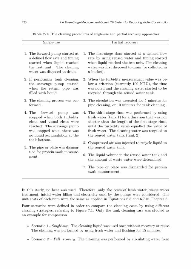
120 7 A Three-Stage Measurement-Based CIP System for Reducing Water Consumption
Table 7.1: The cleaning procedures of single-use and partial recovery approaches
Single-use Partial recovery
1. The forward pump started ata defined flow rate and timingstarted when liquid reachedthe test unit. The cleaningwater was disposed to drain.
2. If performing tank cleaning,the scavenge pump startedwhen the return pipe wasfilled with liquid.
3. The cleaning process was per-formed.
4. The forward pump wasstopped when both turbidityclean and visual clean werereached. The scavenge pumpwas stopped when there wasno liquid accumulation at thetank bottom.
5. The pipe or plate was disman-tled for protein swab measure-ment.
1. The first-stage rinse started at a defined flowrate by using reused water and timing startedwhen liquid reached the test unit. The cleaningwater was first disposed to drain (or collected ina bucket).
2. When the turbidity measurement value was be-low a criterion (currently 100 NTU), the timewas noted and the cleaning water started to berecycled through the reused water tank.
3. The circulation was executed for 5 minutes forpipe cleaning, or 10 minutes for tank cleaning.
4. The third stage rinse was performed by usingfresh water (tank 1) for a duration that was notshorter than the length of the first stage rinse,until the turbidity value equalled the value offresh water. The cleaning water was recycled tothe reused water tank (tank 2).
5. Compressed air was injected to recycle liquid tothe reused water tank.
6. The liquid volume in the reused water tank andthe amount of waste water were determined.
7. The pipe or plate was dismantled for proteinswab measurement.
In this study, no heat was used. Therefore, only the costs of fresh water, waste watertreatment, initial water filling and electricity used by the pumps were considered. Theunit costs of each item were the same as applied in Equations 6.5 and 6.7 in Chapter 6.
Four scenarios were defined in order to compare the cleaning costs by using differentcleaning strategies, referring to Figure 7.1. Only the tank cleaning case was studied asan example for comparison.
• Scenario 1 - Single-use: The cleaning liquid was used once without recovery or reuse.The cleaning was performed by using fresh water and flushing for 15 minutes.
• Scenario 2 – Full recovery: The cleaning was performed by circulating water from
7.3 Results and Discussion 121
the reused water tank for 10 minutes. A final rinse was conducted by rinsing withfresh water for 5 minutes. All liquid was recovered.
• Scenario 3 – Time-based partial recovery: The three-stage partial recovery approachwas applied. But there were no turbidity measurements to determine the rinsingtime. The times for the first and third stages were both 5 minutes, which madesense because in industrial practices this time was set based on experience and thevalue was larger than the real demand. The circulation time was 10 minutes.
• Scenario 4 – Measurement-based partial recovery: The three-stage partial recoveryapproach used turbidity measurements to determine the rinsing time of the firststage. The third stage rinsing time corresponded to the first stage time. Thisscenario was the same as the partial recovery approach shown in Table 7.1.
7.3 Results and Discussion
7.3.1 Cleaning Time Against Flow RateIn order to implement measurement-based CIP, it is desired that the surface is completelyclean when the turbidity sensor detects a clear signal. In other words, the turbiditycleaning time should not be less than the visual cleaning time or even the protein cleaningtime. Otherwise, the cleaning will stop erroneously even though the surface is still dirty.
The use of high flow velocities improves the cleaning performance and shortens the clean-ing time by intensifying the local wall shear stress [102]. As shown in Figure 7.3A forpipe cleaning, the visual cleaning time at low velocity is much longer than the turbiditycleaning time, meaning that there are still harsh soils on the surface even though the bulkliquid is turbidity clear. The difference between visual cleaning time and turbidity clean-ing time reduces with the increase in flow velocity. The turbidity cleaning time becomeslarger than the visual cleaning time when the velocity is above 0.95 m/s, correspondingto a Reynolds number of 29,000. A further increase in flow velocity does not significantlycontribute to reducing the cleaning time. The cleaning of SS pipes cannot be visuallymonitored on-line. However, when dismantling the SS pipes when the turbidity cleanstatus is reached, large pieces of soils can still be observed on the inner pipe surface, asshown in Table 7.2. It means that for SS pipes the visual cleaning time is longer than theturbidity cleaning time, even at the largest investigated flow velocity. This attributes tothe higher adhesion force of soil materials to the stainless steel surfaces than to PVC [177].However, even though both the turbidity and visual clean status are finally achieved, theswab tests reveal that there are still protein traces remaining on the surfaces. Therefore,an even longer cleaning time is required than both turbidity and visual cleaning times inorder to obtain complete cleanliness.
The turbidity cleaning times of plates are shown in Figure 7.3B. At 1 m3/h, the turbiditycleaning time for PVC plate is shorter than for the stainless steel plate due to the tighteradhesion of the chosen soil on the SS surface [177]. However, the difference becomesinsignificant at higher flow rates, which is in line with the observations in pipe cleaning
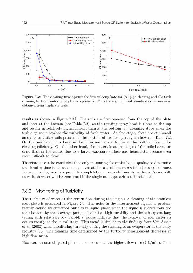
122 7 A Three-Stage Measurement-Based CIP System for Reducing Water Consumption
Figure 7.3: The cleaning time against the flow velocity/rate for (A) pipe cleaning and (B) tankcleaning by fresh water in single-use approach. The cleaning time and standard deviation wereobtained from triplicate tests.
results as shown in Figure 7.3A. The soils are first removed from the top of the plateand later at the bottom (see Table 7.2), as the rotating spray head is closer to the topand results in relatively higher impact than at the bottom [6]. Cleaning stops when theturbidity value reaches the turbidity of fresh water. At this stage, there are still smallamounts of visible soils present at the bottom of the test plates, as shown in Table 7.2.On the one hand, it is because the lower mechanical forces at the bottom impact thecleaning efficiency. On the other hand, the materials at the edges of the soiled area aredrier than in the center due to a larger exposure surface and henceforth become evenmore difficult to clean.
Therefore, it can be concluded that only measuring the outlet liquid quality to determinethe cleaning time is not safe enough even at the largest flow rate within the studied range.Longer cleaning time is required to completely remove soils from the surfaces. As a result,more fresh water will be consumed if the single-use approach is still retained.
7.3.2 Monitoring of TurbidityThe turbidity of water at the return flow during the single-use cleaning of the stainlesssteel plate is presented in Figure 7.4. The noise in the measurement signals is predom-inantly caused by entrained bubbles in liquid phase when the liquid is sucked from thetank bottom by the scavenge pump. The initial high turbidity and the subsequent longtailing with relatively low turbidity values indicate that the removal of soil materialsoccurs mostly at the initial stage. This trend is similar to the findings from Van Asseltet al. (2002) when monitoring turbidity during the cleaning of an evaporator in the dairyindustry [58]. The cleaning time determined by the turbidity measurement decreases athigh flow rates.
However, an unanticipated phenomenon occurs at the highest flow rate (2 L/min). That
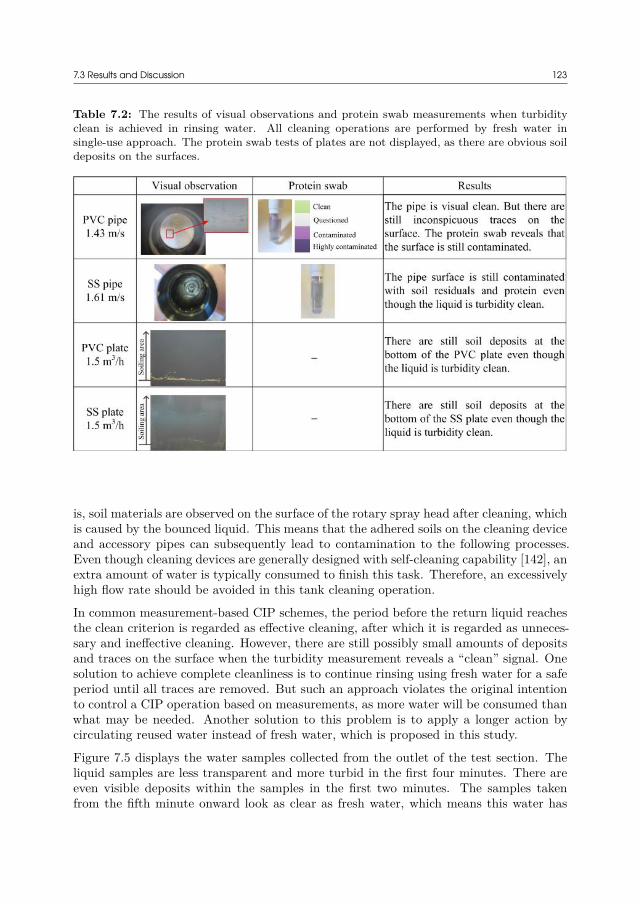
7.3 Results and Discussion 123
Table 7.2: The results of visual observations and protein swab measurements when turbidityclean is achieved in rinsing water. All cleaning operations are performed by fresh water insingle-use approach. The protein swab tests of plates are not displayed, as there are obvious soildeposits on the surfaces.
is, soil materials are observed on the surface of the rotary spray head after cleaning, whichis caused by the bounced liquid. This means that the adhered soils on the cleaning deviceand accessory pipes can subsequently lead to contamination to the following processes.Even though cleaning devices are generally designed with self-cleaning capability [142], anextra amount of water is typically consumed to finish this task. Therefore, an excessivelyhigh flow rate should be avoided in this tank cleaning operation.
In common measurement-based CIP schemes, the period before the return liquid reachesthe clean criterion is regarded as effective cleaning, after which it is regarded as unneces-sary and ineffective cleaning. However, there are still possibly small amounts of depositsand traces on the surface when the turbidity measurement reveals a “clean” signal. Onesolution to achieve complete cleanliness is to continue rinsing using fresh water for a safeperiod until all traces are removed. But such an approach violates the original intentionto control a CIP operation based on measurements, as more water will be consumed thanwhat may be needed. Another solution to this problem is to apply a longer action bycirculating reused water instead of fresh water, which is proposed in this study.
Figure 7.5 displays the water samples collected from the outlet of the test section. Theliquid samples are less transparent and more turbid in the first four minutes. There areeven visible deposits within the samples in the first two minutes. The samples takenfrom the fifth minute onward look as clear as fresh water, which means this water has
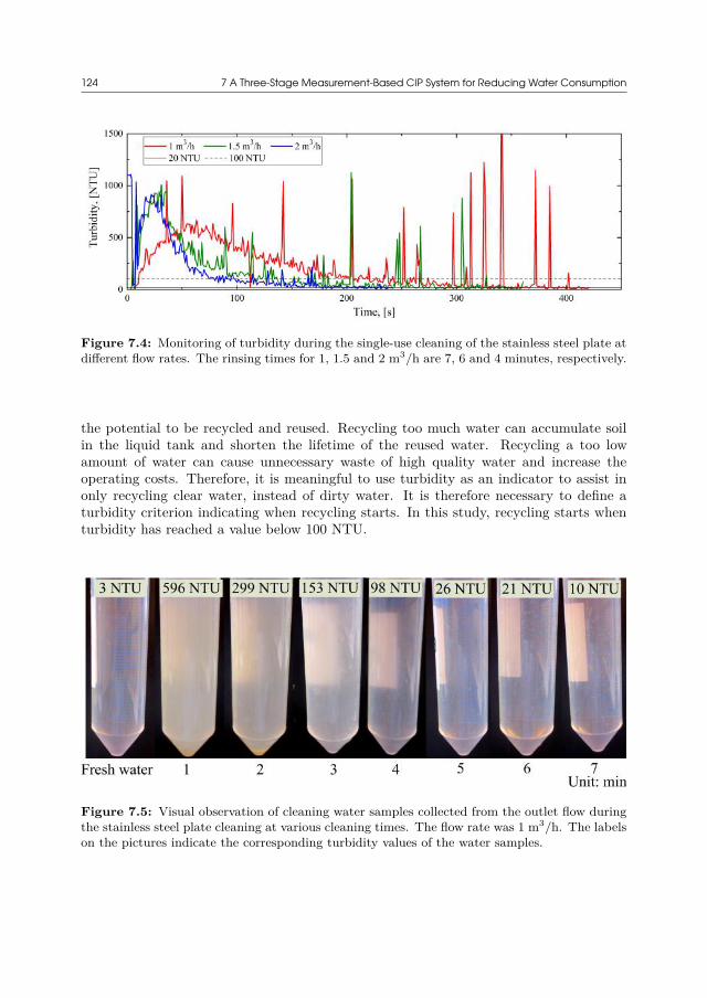
124 7 A Three-Stage Measurement-Based CIP System for Reducing Water Consumption
Figure 7.4: Monitoring of turbidity during the single-use cleaning of the stainless steel plate atdifferent flow rates. The rinsing times for 1, 1.5 and 2 m3/h are 7, 6 and 4 minutes, respectively.
the potential to be recycled and reused. Recycling too much water can accumulate soilin the liquid tank and shorten the lifetime of the reused water. Recycling a too lowamount of water can cause unnecessary waste of high quality water and increase theoperating costs. Therefore, it is meaningful to use turbidity as an indicator to assist inonly recycling clear water, instead of dirty water. It is therefore necessary to define aturbidity criterion indicating when recycling starts. In this study, recycling starts whenturbidity has reached a value below 100 NTU.
Figure 7.5: Visual observation of cleaning water samples collected from the outlet flow duringthe stainless steel plate cleaning at various cleaning times. The flow rate was 1 m3/h. The labelson the pictures indicate the corresponding turbidity values of the water samples.
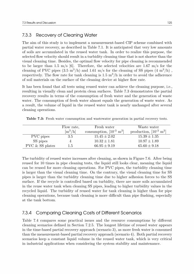
7.3 Results and Discussion 125
7.3.3 Recovery of Cleaning WaterThe aim of this study is to implement a measurement-based CIP scheme combined withpartial water recovery, as described in Table 7.1. It is anticipated that very low amountsof soils are accumulated in the reused water tank. In order to realize this purpose, theselected flow velocity should result in a turbidity cleaning time that is not shorter than thevisual cleaning time. Besides, the optimal flow velocity for pipe cleaning is recommendedto be larger than 1.5 m/s [6]. Therefore, the selected velocities are 1.67 m/s for thecleaning of PVC pipes (3.5 m3/h) and 1.61 m/s for the cleaning of SS pipes (4 m3/h) ,respectively. The flow rate for tank cleaning is 1.5 m3/h in order to avoid the adherenceof soil materials on the surface of the cleaning device at higher flow rate.
It has been found that all tests using reused water can achieve the cleaning purpose, i.e.,resulting in visually clean and protein clean surfaces. Table 7.3 demonstrates the partialrecovery results in terms of the consumption of fresh water and the generation of wastewater. The consumption of fresh water almost equals the generation of waste water. Asa result, the volume of liquid in the reused water tank is nearly unchanged after severalcleaning operations.
Table 7.3: Fresh water consumption and wastewater generation in partial recovery tests.
Flow rate,[m3/h]
Fresh waterconsumption, [10-3 m3]
Waste waterproduction, [10-3 m3]
PVC pipes 3.5 15.45 ± 2.02 15.39 ± 1.35SS pipes 4 10.32 ± 1.81 10.97 ± 1.89
PVC & SS plates 1.5 66.95 ± 9.19 65.60 ± 9.18
The turbidity of reused water increases after cleaning, as shown in Figure 7.6. After beingreused for 10 times in pipe cleaning tests, the liquid still looks clear, meaning the liquidcan be reused for more cleaning operations. For PVC pipes, the turbidity cleaning timeis larger than the visual cleaning time. On the contrary, the visual cleaning time for SSpipes is larger than the turbidity cleaning time due to higher adhesion forces to the SSsurface. If the recycle is controlled based on turbidity, there are more soils accumulatedin the reuse water tank when cleaning SS pipes, leading to higher turbidity values in therecycled liquid. The turbidity of reused water for tank cleaning is higher than for pipecleaning operations, because tank cleaning is more difficult than pipe flushing, especiallyat the tank bottom.
7.3.4 Comparing Cleaning Costs of Different ScenariosTable 7.4 compares some practical issues and the resource consumptions by differentcleaning scenarios defined in Section 7.2.5. The longest lifetime of reused water appearsin the time-based partial recovery approach (scenario 3), as more fresh water is consumedthan the measurement-based partial recovery approach (scenario 4). Both partial recoveryscenarios keep a constant liquid volume in the reused water tank, which is very criticalin industrial applications when considering the system stability and maintenance.
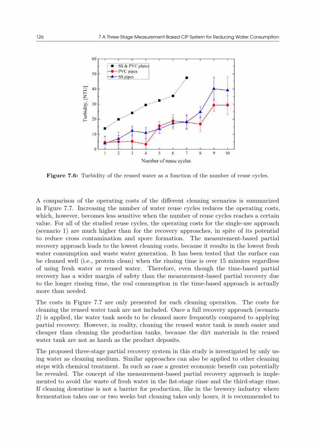
126 7 A Three-Stage Measurement-Based CIP System for Reducing Water Consumption
Figure 7.6: Turbidity of the reused water as a function of the number of reuse cycles.
A comparison of the operating costs of the different cleaning scenarios is summarizedin Figure 7.7. Increasing the number of water reuse cycles reduces the operating costs,which, however, becomes less sensitive when the number of reuse cycles reaches a certainvalue. For all of the studied reuse cycles, the operating costs for the single-use approach(scenario 1) are much higher than for the recovery approaches, in spite of its potentialto reduce cross contamination and spore formation. The measurement-based partialrecovery approach leads to the lowest cleaning costs, because it results in the lowest freshwater consumption and waste water generation. It has been tested that the surface canbe cleaned well (i.e., protein clean) when the rinsing time is over 15 minutes regardlessof using fresh water or reused water. Therefore, even though the time-based partialrecovery has a wider margin of safety than the measurement-based partial recovery dueto the longer rinsing time, the real consumption in the time-based approach is actuallymore than needed.
The costs in Figure 7.7 are only presented for each cleaning operation. The costs forcleaning the reused water tank are not included. Once a full recovery approach (scenario2) is applied, the water tank needs to be cleaned more frequently compared to applyingpartial recovery. However, in reality, cleaning the reused water tank is much easier andcheaper than cleaning the production tanks, because the dirt materials in the reusedwater tank are not as harsh as the product deposits.
The proposed three-stage partial recovery system in this study is investigated by only us-ing water as cleaning medium. Similar approaches can also be applied to other cleaningsteps with chemical treatment. In such as case a greater economic benefit can potentiallybe revealed. The concept of the measurement-based partial recovery approach is imple-mented to avoid the waste of fresh water in the fist-stage rinse and the third-stage rinse.If cleaning downtime is not a barrier for production, like in the brewery industry wherefermentation takes one or two weeks but cleaning takes only hours, it is recommended to

7.3 Results and Discussion 127
Tab
le7.
4:C
ompa
rison
ofta
nkcl
eani
ngfo
rdi
ffere
ntsc
enar
ios.
The
flow
rate
was
1.5
m3 /h
.
Scen
ario
App
roac
h
Num
ber
ofre
quire
dta
nk(s
)
Fres
hwa
ter
cons
umpt
ion,
[kg/
clea
ning
]
Was
tewa
ter
gene
ratio
n,[k
g/cl
ean-
ing]
Tota
lcl
eani
ngtim
e,[m
in/-
clea
ning
]
Liqu
idvo
lum
ein
the
reus
edwa
ter
tank
Turb
idity
ofwa
ter
inth
ere
used
wate
rta
nk
Reu
sed
wate
rlif
etim
e
Ope
ratio
nco
st
1Si
ngle
-use
137
537
515
--
-H
igh
2Fu
llre
cove
ry2
125
015
Incr
ease
dH
ighl
yin
crea
sed
Shor
tIn
term
edia
te
3T
ime-
base
dpa
rtia
lre
cove
ry2
125
125
20U
ncha
nged
Very
slow
lyin
crea
sed
Very
long
Inte
rmed
iate
4M
easu
rem
ent-
base
dpa
rtia
lre
cove
ry2
∼67
∼67
∼16
Unc
hang
edSl
owly
incr
ease
dLo
ngLo
w
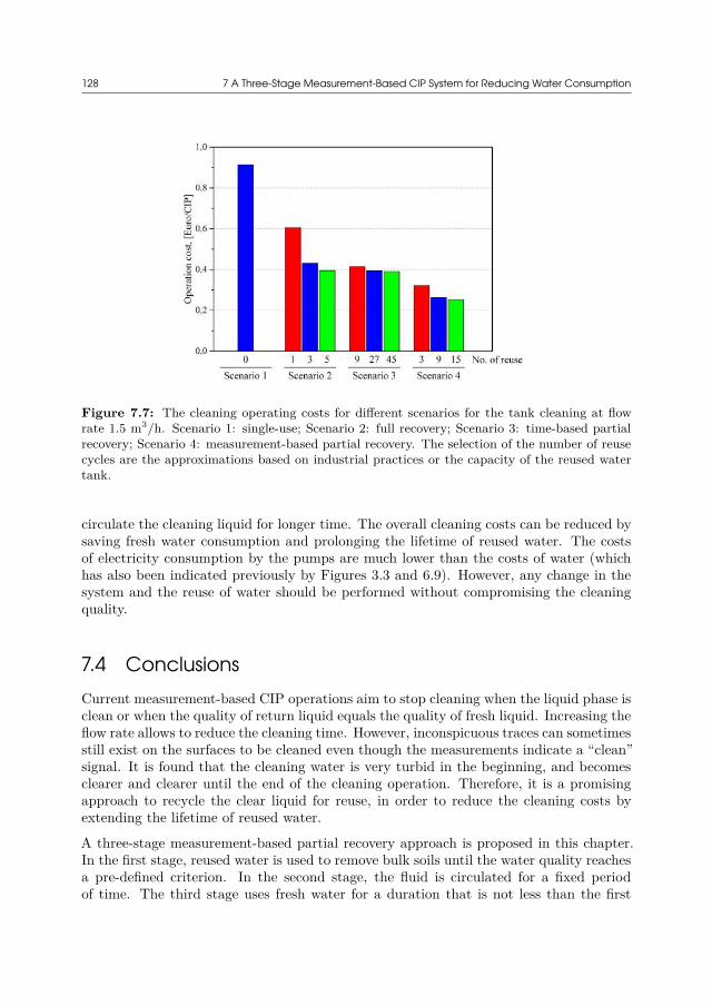
128 7 A Three-Stage Measurement-Based CIP System for Reducing Water Consumption
Figure 7.7: The cleaning operating costs for different scenarios for the tank cleaning at flowrate 1.5 m3/h. Scenario 1: single-use; Scenario 2: full recovery; Scenario 3: time-based partialrecovery; Scenario 4: measurement-based partial recovery. The selection of the number of reusecycles are the approximations based on industrial practices or the capacity of the reused watertank.
circulate the cleaning liquid for longer time. The overall cleaning costs can be reduced bysaving fresh water consumption and prolonging the lifetime of reused water. The costsof electricity consumption by the pumps are much lower than the costs of water (whichhas also been indicated previously by Figures 3.3 and 6.9). However, any change in thesystem and the reuse of water should be performed without compromising the cleaningquality.
7.4 ConclusionsCurrent measurement-based CIP operations aim to stop cleaning when the liquid phase isclean or when the quality of return liquid equals the quality of fresh liquid. Increasing theflow rate allows to reduce the cleaning time. However, inconspicuous traces can sometimesstill exist on the surfaces to be cleaned even though the measurements indicate a “clean”signal. It is found that the cleaning water is very turbid in the beginning, and becomesclearer and clearer until the end of the cleaning operation. Therefore, it is a promisingapproach to recycle the clear liquid for reuse, in order to reduce the cleaning costs byextending the lifetime of reused water.
A three-stage measurement-based partial recovery approach is proposed in this chapter.In the first stage, reused water is used to remove bulk soils until the water quality reachesa pre-defined criterion. In the second stage, the fluid is circulated for a fixed periodof time. The third stage uses fresh water for a duration that is not less than the first

7.4 Conclusions 129
stage, with all water recovered. As a result, the overall cleaning is performed for asufficient period of time without increasing the consumption of fresh water. The watervolume in the reused water tank keeps unchanged. So the cleaning water can be reusedseveral times. The lifetime of the reused cleaning water can be prolonged by avoidingthe accumulation of impurities in the reused water tank. Four scenarios are studied tocompare the operating costs by conducting single-use or recovery approaches. The resultsreveal that the proposed measurement-based partial recovery allows savings between 30-70% of the cleaning costs compared with other approaches.
Even though the proposed approach is developed by only using water as cleaning medium,it is possible to apply this approach to other cleaning steps, where chemical solutionsare used. Especially, the proposed procedure can be used for processes where cleaningdowntime does not restrict the production efficiency.
List of Nomenclature in Chapter 7The following nomenclature is only valid for this chapter. Some symbols are used in otherchapters but with different meanings. Otherwise, the symbols are specifically explainedin the text if there is no nomenclature in some chapter.
Roman LettersNReuse times Number of reuse cycles, dimensionlessw0 Weight of dry pipe, [g]w1 Weight of filled pipe with caps, [g]w2 Weight of filled pipe without caps, [g]wsoil Weight of soil, [g]
Greek Lettersδi Cleaning cost of item i

130
CHAPTER8Cleaning of Toothpastefrom Vessel Surfaces by
Impinging Liquid Jetsand Falling Films
In the work presented in this chapter, the removal of a toothpaste soil from flat glasssurfaces by using impinging liquid jets and falling films were studied. The model forthe adhesive removal of soil layers by impinging water jets presented by Bhagat et al.(2017) [178] was applied to the case of toothpaste removal. This work was performedin collaboration with Professor Ian Wilson at the Department of Chemical Engineeringand Biotechnology at the University of Cambridge in the UK, during my research visitto Ian’s group in the summer of 2018. The author greatly appreciates the thoughtfuldiscussions with Professor Wilson and Ph.D students Rajesh Bhagat, Rubens RosarioFernandes and Melissa Chee in Cambridge.
8.1 IntroductionLiquid jets are widely used in cleaning operations to remove soil materials from internaltank surfaces or open surfaces of process equipment. Common jet devices for tank cleaningoperations include the static spray ball and the rotary jet head, as described in Table 2.3.The selection of a suitable jet device relies on the design and process for which the surfaceis to be cleaned.
The flow pattern and cleaning behaviour associated with a single liquid jet have beeninvestigated. These studies can be mainly categorized into two groups, as discussed inSection 2.5: (i) cleaning in the impingement area generally studies the flow behaviourand cleaning dynamics around the impingement point where the jet hits the surface [78,80, 178, 179]; (ii) cleaning by falling films focuses on cleaning below the impingementpoint where the liquid flows down under gravity and wets a vertical or inclined wall [82,
132 8 Cleaning of Toothpaste from Vessel Surfaces by Impinging Liquid Jets and Falling Films
83].
Wilson et al. (2012) presented a simple model of the radial flow region to predict the hy-draulic jump radius and the minimum width of falling film based on momentum balances[72]. In the model of Wilson et al. (2012), the flow in the radial flow region is treated asa laminar film with parabolic velocity profile, which was revised by Bhagat et al. (2016)to include the development of laminar and turbulent boundary layers in the thin film[73]. The flow model has been used to develop an adhesive removal model to computethe momentum force at the cleaning front of soft-solid soil layers [75] and viscoplastic soillayers [77]. The removal model has been extended to include nozzle movement [76] andan angle of the jet to the wall [180]. Liquid losses due to jet breakup were included in aneffective flow rate term when being applied for industrial tank cleaning [78].
This chapter applies the adhesive removal model reported by Wilson et al. (2014) andBhagat et al. (2017) to the cleaning of a new soil type, namely toothpaste. In addition toconsidering cleaning by static and moving jets, as investigated in previous studies, thischapter develops the model by including the effect of soil soaking, and extends the modelto the cleaning by falling films.
8.2 Model Description
8.2.1 Impinging Jet Introduced Flow PatternsThe flow pattern generated by a horizontal jet impinging on a vertical surface is illustratedin Figure 8.1. A radial flow zone (RFZ) is formed around the impingement point, wherethe liquid moves rapidly outwards and terminates at a hydraulic jump. In the RFZ,the effect of gravity is negligible. So the schematic in Figure 8.1A applies to a verticaljet impinging on a horizontal surface as well. Beyond the RFZ, gravity becomes thedominant force and the liquid flows downwards to result in a transition film zone. Arope or corona with varying thickness forms above the RFZ, containing the liquid fromthe hydraulic jump. The falling film is driven by gravity. It features two regions: (i)the outer bounding flow, which is the extension of the rope above the corona, and (ii)the inner section, here termed the core, of width Wc and thickness less than the rope.Further details of the falling film are given by Wang et al. (2013) [80, 83]. In caseswhere downward momentum is smaller than surface tension, the film width may narrowgradually to a thin tail, called rivulet flow, or the film splits, creating a dry patch (seeFigure 2.5). The formation of different falling film types depends on flow properties andsurface characteristics. In this study, only glass surfaces are used, where water flowsstably out a long distance downwards before narrowing to a tail. Therefore, a pseudostable gravity falling film of constant width is assumed.
The aim of this work was to develop a cleaning rate model for toothpaste, based on theadhesive removal theory reported by Wilson et al. (2014) and Bhagat et al. (2017) [75,178]. The parameters of the model were obtained from the cleaning of soil materials usingstatic impinging jets. Then the model and the parameters were applied to the cleaningof soil using moving jets and falling films.
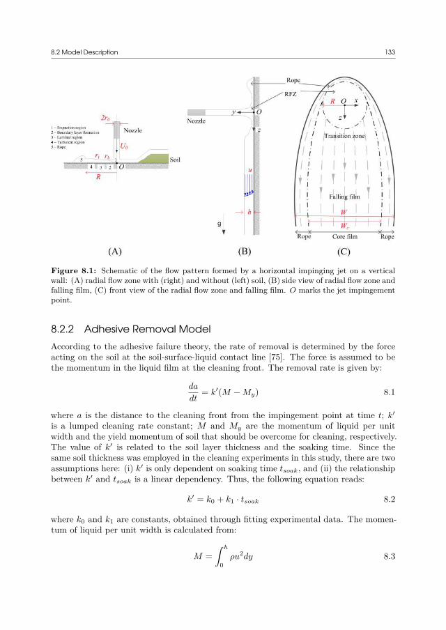
8.2 Model Description 133
Figure 8.1: Schematic of the flow pattern formed by a horizontal impinging jet on a verticalwall: (A) radial flow zone with (right) and without (left) soil, (B) side view of radial flow zone andfalling film, (C) front view of the radial flow zone and falling film. O marks the jet impingementpoint.
8.2.2 Adhesive Removal ModelAccording to the adhesive failure theory, the rate of removal is determined by the forceacting on the soil at the soil-surface-liquid contact line [75]. The force is assumed to bethe momentum in the liquid film at the cleaning front. The removal rate is given by:
da
dt= k′(M − My) 8.1
where a is the distance to the cleaning front from the impingement point at time t; k′
is a lumped cleaning rate constant; M and My are the momentum of liquid per unitwidth and the yield momentum of soil that should be overcome for cleaning, respectively.The value of k′ is related to the soil layer thickness and the soaking time. Since thesame soil thickness was employed in the cleaning experiments in this study, there are twoassumptions here: (i) k′ is only dependent on soaking time tsoak, and (ii) the relationshipbetween k′ and tsoak is a linear dependency. Thus, the following equation reads:
k′ = k0 + k1 · tsoak 8.2
where k0 and k1 are constants, obtained through fitting experimental data. The momen-tum of liquid per unit width is calculated from:
M =∫ h
0ρu2dy 8.3
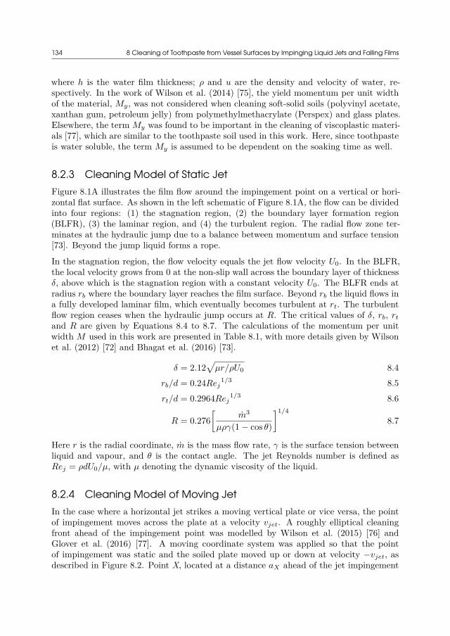
134 8 Cleaning of Toothpaste from Vessel Surfaces by Impinging Liquid Jets and Falling Films
where h is the water film thickness; ρ and u are the density and velocity of water, re-spectively. In the work of Wilson et al. (2014) [75], the yield momentum per unit widthof the material, My, was not considered when cleaning soft-solid soils (polyvinyl acetate,xanthan gum, petroleum jelly) from polymethylmethacrylate (Perspex) and glass plates.Elsewhere, the term My was found to be important in the cleaning of viscoplastic materi-als [77], which are similar to the toothpaste soil used in this work. Here, since toothpasteis water soluble, the term My is assumed to be dependent on the soaking time as well.
8.2.3 Cleaning Model of Static JetFigure 8.1A illustrates the film flow around the impingement point on a vertical or hori-zontal flat surface. As shown in the left schematic of Figure 8.1A, the flow can be dividedinto four regions: (1) the stagnation region, (2) the boundary layer formation region(BLFR), (3) the laminar region, and (4) the turbulent region. The radial flow zone ter-minates at the hydraulic jump due to a balance between momentum and surface tension[73]. Beyond the jump liquid forms a rope.
In the stagnation region, the flow velocity equals the jet flow velocity U0. In the BLFR,the local velocity grows from 0 at the non-slip wall across the boundary layer of thicknessδ, above which is the stagnation region with a constant velocity U0. The BLFR ends atradius rb where the boundary layer reaches the film surface. Beyond rb the liquid flows ina fully developed laminar film, which eventually becomes turbulent at rt. The turbulentflow region ceases when the hydraulic jump occurs at R. The critical values of δ, rb, rt
and R are given by Equations 8.4 to 8.7. The calculations of the momentum per unitwidth M used in this work are presented in Table 8.1, with more details given by Wilsonet al. (2012) [72] and Bhagat et al. (2016) [73].
δ = 2.12√
µr/ρU0 8.4rb/d = 0.24Rej
1/3 8.5rt/d = 0.2964Rej
1/3 8.6
R = 0.276[
m3
µργ(1 − cos θ)
]1/4
8.7
Here r is the radial coordinate, m is the mass flow rate, γ is the surface tension betweenliquid and vapour, and θ is the contact angle. The jet Reynolds number is defined asRej = ρdU0/µ, with µ denoting the dynamic viscosity of the liquid.
8.2.4 Cleaning Model of Moving JetIn the case where a horizontal jet strikes a moving vertical plate or vice versa, the pointof impingement moves across the plate at a velocity vjet. A roughly elliptical cleaningfront ahead of the impingement point was modelled by Wilson et al. (2015) [76] andGlover et al. (2016) [77]. A moving coordinate system was applied so that the pointof impingement was static and the soiled plate moved up or down at velocity −vjet, asdescribed in Figure 8.2. Point X, located at a distance aX ahead of the jet impingement
8.2 Model Description 135T
able
8.1:
Sum
mar
yof
equa
tions
for
calc
ulat
ing
film
thic
knes
sh
,sur
face
velo
city
Us,v
eloc
itypr
ofile
uan
dm
omen
tum
per
unit
wid
thM
inth
era
dial
flow
zone
whe
ncl
eani
ngby
stat
icje
t.T
heeq
uatio
nsar
ede
rived
acco
rdin
gto
Bha
gat
etal
.(20
16)
[73]
.
Reg
ions
h,U
san
du
Mom
entu
mpe
run
itw
idth
M
BLFR
r<
r b
h=
0.12
5/r
+1.
06(r
d/R
e j)1/
2
Us
=U
0
u=
{ U0f
(η)
y<
δ
U0
y≥
δ
M=
ρU
02 h−
ρU
02 δ(C
1−
1)
Lam
inar
r b<
r<
r t
h=
d
[ 3.79
2R
e j
( r d
) 2 +0.
1975
( d r
)]U
s=
U0
8C2
hr
d2
u=
Usf
(η)
M=
C1ρ
Us
2 h
Turb
ulen
tr t
<r
<R
h=
0.02
09d
Re j
1/4
( r d
) 5/4+
(0.2
96−
0.00
1356
Re j
1/2 )( d
2 r
)U
s=
4Q 7πrh
u=
Usη
1/7
M=
ρ64 63
Q 2πU
0
r
[ 0.16
7R
ej
0.12
5(r d
)9/
4+
(2.3
7−0.
0108
Re
j1/
2)]
The
equa
tions
used
for
calc
ulat
ion
η=
y/δ
f(η
)=η
−3 2η
2+
4η3
−5 2η
4C
1=
∫ 1 0f
(η)2 d
ηC
2=
∫ 1 0f
(η)d
η
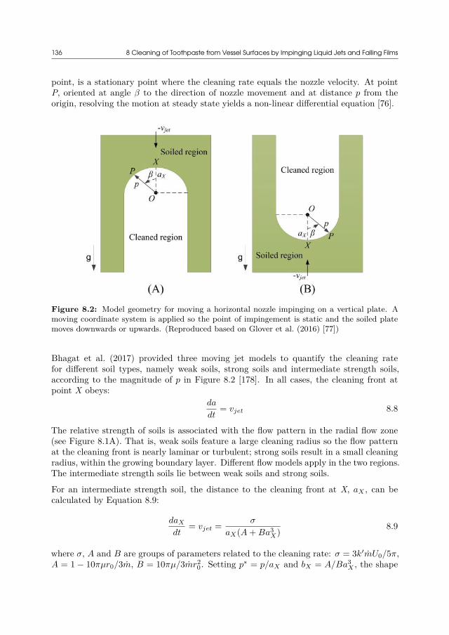
136 8 Cleaning of Toothpaste from Vessel Surfaces by Impinging Liquid Jets and Falling Films
point, is a stationary point where the cleaning rate equals the nozzle velocity. At pointP, oriented at angle β to the direction of nozzle movement and at distance p from theorigin, resolving the motion at steady state yields a non-linear differential equation [76].
Figure 8.2: Model geometry for moving a horizontal nozzle impinging on a vertical plate. Amoving coordinate system is applied so the point of impingement is static and the soiled platemoves downwards or upwards. (Reproduced based on Glover et al. (2016) [77])
Bhagat et al. (2017) provided three moving jet models to quantify the cleaning ratefor different soil types, namely weak soils, strong soils and intermediate strength soils,according to the magnitude of p in Figure 8.2 [178]. In all cases, the cleaning front atpoint X obeys:
da
dt= vjet 8.8
The relative strength of soils is associated with the flow pattern in the radial flow zone(see Figure 8.1A). That is, weak soils feature a large cleaning radius so the flow patternat the cleaning front is nearly laminar or turbulent; strong soils result in a small cleaningradius, within the growing boundary layer. Different flow models apply in the two regions.The intermediate strength soils lie between weak soils and strong soils.
For an intermediate strength soil, the distance to the cleaning front at X, aX , can becalculated by Equation 8.9:
daX
dt= vjet = σ
aX(A + Ba3X)
8.9
where σ, A and B are groups of parameters related to the cleaning rate: σ = 3k′mU0/5π,A = 1 − 10πµr0/3m, B = 10πµ/3mr2
0. Setting p∗ = p/aX and bX = A/Ba3X , the shape
8.2 Model Description 137
of the cleaning front can be written in a dimensionless form as:dp∗
dβ= 1
sin β
(bX + 1
bX + p∗3
)− p∗
tan β8.10
The initial condition is that p∗ = 1 at β = 0. The only unknown parameter neededto solve Equation 8.10 is the cleaning rate constant k′, which can come either from theinspection of data generated by a static cleaning nozzle or by fitting the experimentalresults of the cleaning by moving jets. The cleaning models for other soil strengths canbe found in Bhagat et al. (2017) [178].
8.2.5 Cleaning Model of Falling FilmThe falling film is assumed to be laminar flow with a parabolic velocity profile:
u = ρg
2µ(2hy − y2) 8.11
The average velocity in the film (Uav) is:
Uav = 1h
∫ h
0udy = ρgh2
3µ8.12
Based on Equations 8.3, 8.11 and 8.12, the momentum of film per unit width can becalculated via:
M = 65
ρU2avh 8.13
The water film thickness h can be calculated based on some assumptions. In Nusselt’stheory, the film is purely viscous so a flat surface is assumed [84]. The mean film thicknessis:
hNusselt =(
3µq
ρg
)1/3
8.14
where q is the volumetric flow rate per unit width; g is the gravitational accelerationterm. The right term in Equation 8.14 can be re-written as the wetting rate of a fallingfilm according to Equation 2.1. However, it has been found that wave inception occursto liquid at a low flow rate. According to Kapitza’s theory of wavy flow, the parabolicvelocity profile also applies but the mean film thickness is given by [85]:
hKapitza =(
2.4µq
ρg
)1/3
≈ 0.928hNusselt 8.15
Therefore, based on Equations 8.14 and 8.15, the Nusselt film is ca. 7% thicker than theKapitza film. For water, Nusselt’s and Kapitza’s theories are valid when the film Reynoldsnumber (Ref = 4ρq/µ) is less than 1,160 [85]. Since ropes exist on both edges of thefalling film, with a thickness much larger than the core film (as indicated in Figure 8.1C),only the momentum per unit width in the core film region is calculated. In the core film,the volumetric flow rate per unit width q is estimated by q = fcQ/Wc, where the widthof core film Wc comes from experimental observations. The fraction of volumetric flowrate in the core film fc is assumed to be 50% of the overall volumetric flow rate Q byignoring flow splash [80].
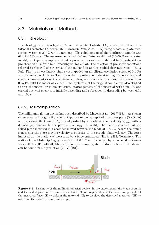
138 8 Cleaning of Toothpaste from Vessel Surfaces by Impinging Liquid Jets and Falling Films
8.3 Materials and Methods
8.3.1 RheologyThe rheology of the toothpaste (Advanced White, Colgate, US) was measured on a ro-tational rheometer (Kinexus lab+, Malvern Panalytical, UK) using a parallel plate mea-suring system at 20 °C with 1 mm gap. The solid content of the toothpaste sample was62.1±4.5 % w/w. The measurements included undiluted or diluted (10–50 % extra waterweight) toothpaste samples without a pre-shear, as well as undiluted toothpaste with apre-shear at 5 Pa for 3 min (referring to Table 8.3). The selection of pre-shear conditionsreferred to the wall shear stress of the falling film at the studied flow rate range (ca. 3Pa). Firstly, an oscillatory time sweep applied an amplitude oscillation stress of 0.1 Paat a frequency of 1 Hz for 3 min in order to probe the understanding of the viscous andelastic characteristics of the materials. Then, a stress sweep increased the stress from0.25 Pa until the material yielded. The hysteresis of the original sample was also studiedto test the macro- or micro-structural rearrangement of the material with time. It wascarried out with shear rate initially ascending and subsequently descending between 0.01and 100 s-1.
8.3.2 MillimanipulationThe millimanipulation device has been described by Magens et al. (2017) [181]. As shownschematically in Figure 8.3, the toothpaste sample was spread on a glass plate (5 × 5 cm)with a known thickness of δsoil, and pushed by a blade at a set velocity vblade with adefined gap distance to the plate surface δgap. In reality, the blade was static but thesoiled plate mounted in a chamber moved towards the blade at −vblade, where the minussign means the plate moving velocity is opposite to the pseudo blade velocity. The forceimposed on the blade was measured by a force transducer (HBM S2M, Germany). Thewidth of the blade tip Wblade was 0.140 ± 0.017 mm, scanned by a confocal thicknesssensor (CTS, IFS 2405-3, Micro-Epsilon, Germany) system. More details of the devicecan be found in Magens et al. (2017) [181].
Figure 8.3: Schematic of the millimanipulation device. In the experiments, the blade is staticand the soiled plate moves towards the blade. Three regions denote the three components ofthe measured force: (I) to deform the material, (II) to displace the deformed material, (III) toovercome the shear resistance in the gap.
8.3 Materials and Methods 139
Millimanipulation was performed to investigate the removal force by varying soil thickness,gap distance, and soil types (soaked or not). Measurements were made at different bladevelocities (0.1, 1, 5 and 10 mm/s). To prepare the soaked soil sample, the chamber wherethe soiled plate was mounted was filled with deionized water and emptied immediatelyafter 3 min using a syringe. In the measurement, the soil deformed and accumulated infront of the blade, as indicated in Figure 8.3. The force measured by the sensor includedthree components: (i) that to deform materials ahead of the blade, (ii) that to displacethe deformed materials, and (iii) that to overcome the shear resistance under the tip ofthe blade. The shear force per unit width (region III in Figure 8.3), FW, shear, could bedetermined through the shear stress (τ) by:
FW, shear = τAblade
Lblade= ηappγLbladeWblade
Lblade= ηappγWblade 8.16
where the apparent viscosity ηapp was read from the rheology measurement at a givenapparent shear rate γ = vblade/δgap. Ablade and Lblade were the area and the length of theblade tip, respectively. The combined force of deforming and displacing the soil materialsahead of the blade was defined as the normal force (regions I and II in Figure 8.3),determined by:
FW, normal = FW − FW, shear 8.17
The design of the experiments in the millimanipulation test is shown in Table 8.2.
Table 8.2: Investigated millimanipulation test conditions. All tests were made at differentblade velocities from 0.1 to 10 mm/s.
Investigated parameters Fixed parameters Varied parameters
Soil thickness Soil: original toothpasteδgap = 100 µm δsoil =200, 500, 700 µm
Gap distance Soil: original toothpasteδsoil = 500 µm δgap =50, 100, 200, 400 µm
Soil type δgap = 50 µm Soil: original toothpaste andδsoil = 500 µm toothpaste soaked for 3 min
8.3.3 Impinging Jet Apparatus and Experimental DesignThe pilot-scale apparatus has been previously described by Glover et al. (2016) [77]. Thetest plates were transparent glasses (360 × 600 mm, 150 × 150 mm), which were used asvertical or horizontal walls, respectively. The plates were coated by toothpaste beforebeing mounted prior to cleaning. Even soil layers were prepared by dragging a blade overthe plate with fixed and known clearance between the blade and the plate. The resultingsoil layers were approximately 500 µm thick and a mass coverage 0.059 ± 0.004 g/cm2 onthe plates.
Cleaning experiments were performed immediately (with ca. 3 min preparation) aftersoiling in order to avoid drying. Cleaning was performed with water jets generated
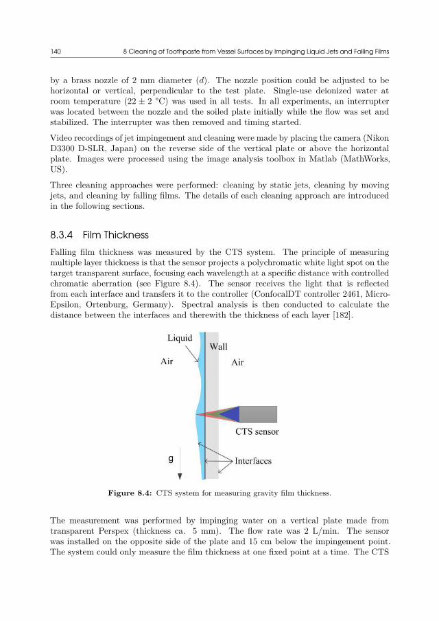
140 8 Cleaning of Toothpaste from Vessel Surfaces by Impinging Liquid Jets and Falling Films
by a brass nozzle of 2 mm diameter (d). The nozzle position could be adjusted to behorizontal or vertical, perpendicular to the test plate. Single-use deionized water atroom temperature (22 ± 2 °C) was used in all tests. In all experiments, an interrupterwas located between the nozzle and the soiled plate initially while the flow was set andstabilized. The interrupter was then removed and timing started.
Video recordings of jet impingement and cleaning were made by placing the camera (NikonD3300 D-SLR, Japan) on the reverse side of the vertical plate or above the horizontalplate. Images were processed using the image analysis toolbox in Matlab (MathWorks,US).
Three cleaning approaches were performed: cleaning by static jets, cleaning by movingjets, and cleaning by falling films. The details of each cleaning approach are introducedin the following sections.
8.3.4 Film ThicknessFalling film thickness was measured by the CTS system. The principle of measuringmultiple layer thickness is that the sensor projects a polychromatic white light spot on thetarget transparent surface, focusing each wavelength at a specific distance with controlledchromatic aberration (see Figure 8.4). The sensor receives the light that is reflectedfrom each interface and transfers it to the controller (ConfocalDT controller 2461, Micro-Epsilon, Ortenburg, Germany). Spectral analysis is then conducted to calculate thedistance between the interfaces and therewith the thickness of each layer [182].
Figure 8.4: CTS system for measuring gravity film thickness.
The measurement was performed by impinging water on a vertical plate made fromtransparent Perspex (thickness ca. 5 mm). The flow rate was 2 L/min. The sensorwas installed on the opposite side of the plate and 15 cm below the impingement point.The system could only measure the film thickness at one fixed point at a time. The CTS
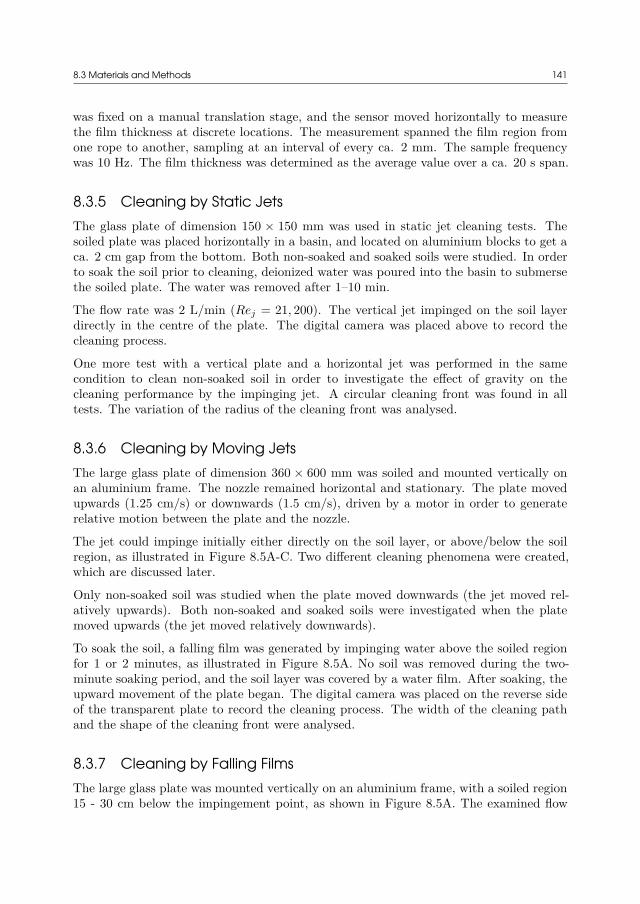
8.3 Materials and Methods 141
was fixed on a manual translation stage, and the sensor moved horizontally to measurethe film thickness at discrete locations. The measurement spanned the film region fromone rope to another, sampling at an interval of every ca. 2 mm. The sample frequencywas 10 Hz. The film thickness was determined as the average value over a ca. 20 s span.
8.3.5 Cleaning by Static JetsThe glass plate of dimension 150 × 150 mm was used in static jet cleaning tests. Thesoiled plate was placed horizontally in a basin, and located on aluminium blocks to get aca. 2 cm gap from the bottom. Both non-soaked and soaked soils were studied. In orderto soak the soil prior to cleaning, deionized water was poured into the basin to submersethe soiled plate. The water was removed after 1–10 min.
The flow rate was 2 L/min (Rej = 21, 200). The vertical jet impinged on the soil layerdirectly in the centre of the plate. The digital camera was placed above to record thecleaning process.
One more test with a vertical plate and a horizontal jet was performed in the samecondition to clean non-soaked soil in order to investigate the effect of gravity on thecleaning performance by the impinging jet. A circular cleaning front was found in alltests. The variation of the radius of the cleaning front was analysed.
8.3.6 Cleaning by Moving JetsThe large glass plate of dimension 360 × 600 mm was soiled and mounted vertically onan aluminium frame. The nozzle remained horizontal and stationary. The plate movedupwards (1.25 cm/s) or downwards (1.5 cm/s), driven by a motor in order to generaterelative motion between the plate and the nozzle.
The jet could impinge initially either directly on the soil layer, or above/below the soilregion, as illustrated in Figure 8.5A-C. Two different cleaning phenomena were created,which are discussed later.
Only non-soaked soil was studied when the plate moved downwards (the jet moved rel-atively upwards). Both non-soaked and soaked soils were investigated when the platemoved upwards (the jet moved relatively downwards).
To soak the soil, a falling film was generated by impinging water above the soiled regionfor 1 or 2 minutes, as illustrated in Figure 8.5A. No soil was removed during the two-minute soaking period, and the soil layer was covered by a water film. After soaking, theupward movement of the plate began. The digital camera was placed on the reverse sideof the transparent plate to record the cleaning process. The width of the cleaning pathand the shape of the cleaning front were analysed.
8.3.7 Cleaning by Falling FilmsThe large glass plate was mounted vertically on an aluminium frame, with a soiled region15 - 30 cm below the impingement point, as shown in Figure 8.5A. The examined flow
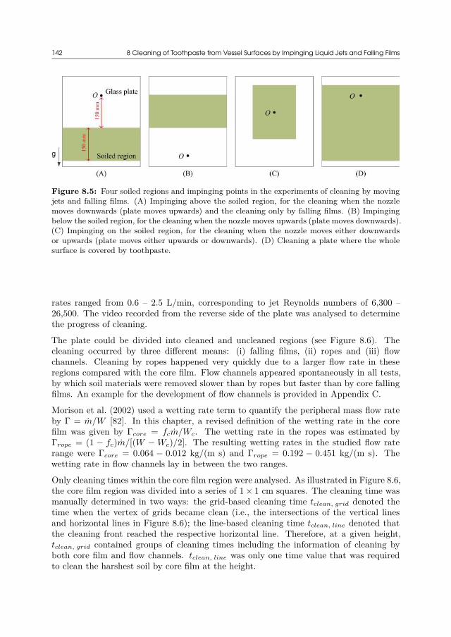
142 8 Cleaning of Toothpaste from Vessel Surfaces by Impinging Liquid Jets and Falling Films
Figure 8.5: Four soiled regions and impinging points in the experiments of cleaning by movingjets and falling films. (A) Impinging above the soiled region, for the cleaning when the nozzlemoves downwards (plate moves upwards) and the cleaning only by falling films. (B) Impingingbelow the soiled region, for the cleaning when the nozzle moves upwards (plate moves downwards).(C) Impinging on the soiled region, for the cleaning when the nozzle moves either downwardsor upwards (plate moves either upwards or downwards). (D) Cleaning a plate where the wholesurface is covered by toothpaste.
rates ranged from 0.6 – 2.5 L/min, corresponding to jet Reynolds numbers of 6,300 –26,500. The video recorded from the reverse side of the plate was analysed to determinethe progress of cleaning.
The plate could be divided into cleaned and uncleaned regions (see Figure 8.6). Thecleaning occurred by three different means: (i) falling films, (ii) ropes and (iii) flowchannels. Cleaning by ropes happened very quickly due to a larger flow rate in theseregions compared with the core film. Flow channels appeared spontaneously in all tests,by which soil materials were removed slower than by ropes but faster than by core fallingfilms. An example for the development of flow channels is provided in Appendix C.
Morison et al. (2002) used a wetting rate term to quantify the peripheral mass flow rateby Γ = m/W [82]. In this chapter, a revised definition of the wetting rate in the corefilm was given by Γcore = fcm/Wc. The wetting rate in the ropes was estimated byΓrope = (1 − fc)m/[(W − Wc)/2]. The resulting wetting rates in the studied flow raterange were Γcore = 0.064 − 0.012 kg/(m s) and Γrope = 0.192 − 0.451 kg/(m s). Thewetting rate in flow channels lay in between the two ranges.
Only cleaning times within the core film region were analysed. As illustrated in Figure 8.6,the core film region was divided into a series of 1 × 1 cm squares. The cleaning time wasmanually determined in two ways: the grid-based cleaning time tclean, grid denoted thetime when the vertex of grids became clean (i.e., the intersections of the vertical linesand horizontal lines in Figure 8.6); the line-based cleaning time tclean, line denoted thatthe cleaning front reached the respective horizontal line. Therefore, at a given height,tclean, grid contained groups of cleaning times including the information of cleaning byboth core film and flow channels. tclean, line was only one time value that was requiredto clean the harshest soil by core film at the height.
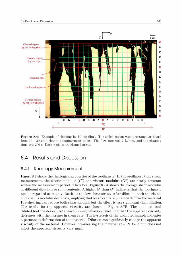
8.4 Results and Discussion 143
Figure 8.6: Example of cleaning by falling films. The soiled region was a rectangular boardfrom 15 - 30 cm below the impingement point. The flow rate was 2 L/min, and the cleaningtime was 200 s. Dark regions are cleaned areas.
8.4 Results and Discussion
8.4.1 Rheology MeasurementFigure 8.7 shows the rheological properties of the toothpaste. In the oscillatory time sweepmeasurement, the elastic modulus (G′) and viscous modulus (G′′) are nearly constantwithin the measurement period. Therefore, Figure 8.7A shows the average shear modulusat different dilutions or solid contents. A higher G′ than G′′ indicates that the toothpastecan be regarded as mainly elastic at the low shear stress. After dilution, both the elasticand viscous modulus decreases, implying that less force is required to deform the material.Pre-shearing can reduce both shear moduli, but the effect is less significant than dilution.The results for the apparent viscosity are shown in Figure 8.7B. The undiluted anddiluted toothpastes exhibit shear thinning behaviour, meaning that the apparent viscositydecreases with the increase in shear rate. The hysteresis of the undiluted sample indicatesa permanent deformation of the material. Dilution can significantly change the apparentviscosity of the material. However, pre-shearing the material at 5 Pa for 3 min does notaffect the apparent viscosity very much.
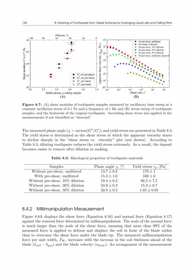
144 8 Cleaning of Toothpaste from Vessel Surfaces by Impinging Liquid Jets and Falling Films
Figure 8.7: (A) shear modulus of toothpaste samples measured by oscillatory time sweep at aconstant oscillation stress of 0.1 Pa and a frequency of 1 Hz and (B) stress sweep of toothpastesamples, and the hysteresis of the original toothpaste. Ascending shear stress was applied in themeasurements if not identified as “descend”.
The measured phase angle (χ = arctan(G′′/G′)) and yield stress are presented in Table 8.3.The yield stress is determined as the shear stress at which the apparent viscosity startsto decline sharply in the “shear stress vs. viscosity” plot (not shown). According toTable 8.3, diluting toothpaste reduces the yield stress extremely. As a result, the depositbecomes easier to remove after dilution or soaking.
Table 8.3: Rheological properties of toothpaste materials
Samples Phase angle χ, [°] Yield stress τy, [Pa]Without pre-shear, undiluted 13.7 ± 0.8 179 ± 1
With pre-shear, undiluted 15.2 ± 1.6 160 ± 6Without pre-shear, 10% dilution 19.4 ± 0.2 66.5 ± 7.5Without pre-shear, 30% dilution 24.9 ± 0.3 15.3 ± 0.7Without pre-shear, 50% dilution 32.8 ± 0.2 1.65 ± 0.05
8.4.2 Millimanipulation MeasurementFigure 8.8A displays the shear force (Equation 8.16) and normal force (Equation 8.17)against the removal force determined by millimanipulation. The scale of the normal forceis much larger than the scale of the shear force, meaning that more than 99% of themeasured force is applied to deform and displace the soil in front of the blade ratherthan to overcome the shear force under the blade tip. The measured millimanipulationforce per unit width, FW , increases with the increase in the soil thickness ahead of theblade (δsoil − δgap) and the blade velocity (vblade). An arrangement of the measurement
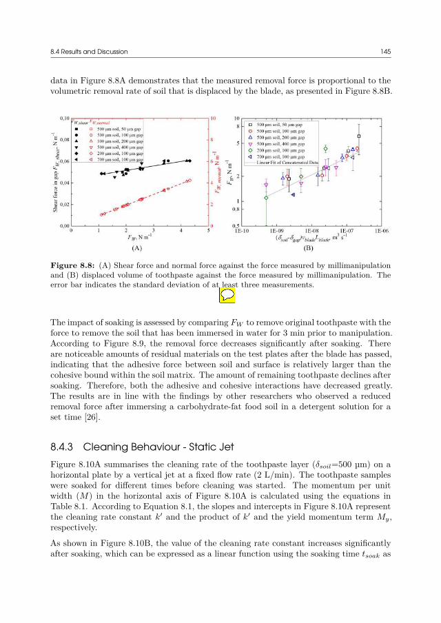
8.4 Results and Discussion 145
data in Figure 8.8A demonstrates that the measured removal force is proportional to thevolumetric removal rate of soil that is displaced by the blade, as presented in Figure 8.8B.
Figure 8.8: (A) Shear force and normal force against the force measured by millimanipulationand (B) displaced volume of toothpaste against the force measured by millimanipulation. Theerror bar indicates the standard deviation of at least three measurements.
The impact of soaking is assessed by comparing FW to remove original toothpaste with theforce to remove the soil that has been immersed in water for 3 min prior to manipulation.According to Figure 8.9, the removal force decreases significantly after soaking. Thereare noticeable amounts of residual materials on the test plates after the blade has passed,indicating that the adhesive force between soil and surface is relatively larger than thecohesive bound within the soil matrix. The amount of remaining toothpaste declines aftersoaking. Therefore, both the adhesive and cohesive interactions have decreased greatly.The results are in line with the findings by other researchers who observed a reducedremoval force after immersing a carbohydrate-fat food soil in a detergent solution for aset time [26].
8.4.3 Cleaning Behaviour - Static JetFigure 8.10A summarises the cleaning rate of the toothpaste layer (δsoil=500 µm) on ahorizontal plate by a vertical jet at a fixed flow rate (2 L/min). The toothpaste sampleswere soaked for different times before cleaning was started. The momentum per unitwidth (M) in the horizontal axis of Figure 8.10A is calculated using the equations inTable 8.1. According to Equation 8.1, the slopes and intercepts in Figure 8.10A representthe cleaning rate constant k′ and the product of k′ and the yield momentum term My,respectively.
As shown in Figure 8.10B, the value of the cleaning rate constant increases significantlyafter soaking, which can be expressed as a linear function using the soaking time tsoak as
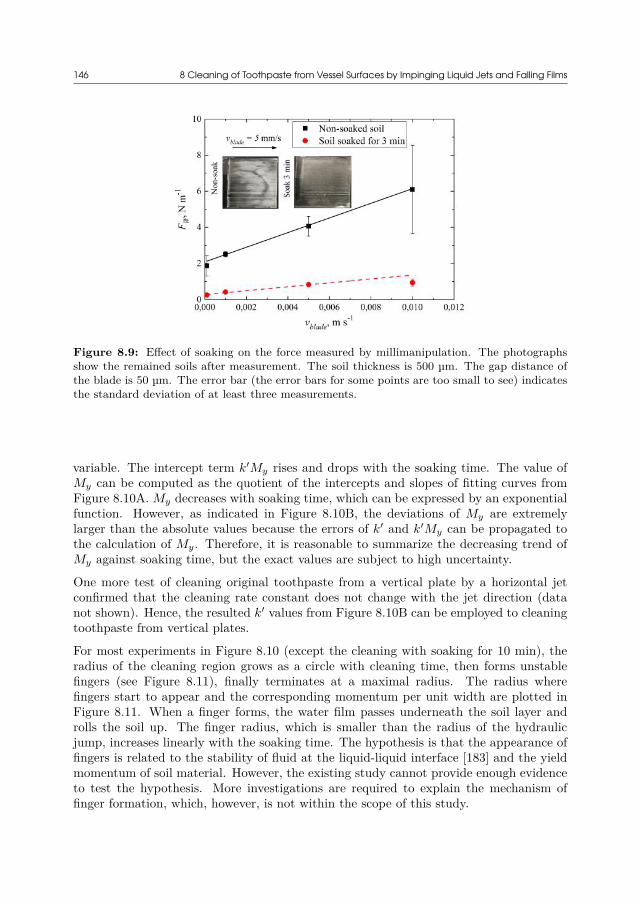
146 8 Cleaning of Toothpaste from Vessel Surfaces by Impinging Liquid Jets and Falling Films
Figure 8.9: Effect of soaking on the force measured by millimanipulation. The photographsshow the remained soils after measurement. The soil thickness is 500 µm. The gap distance ofthe blade is 50 µm. The error bar (the error bars for some points are too small to see) indicatesthe standard deviation of at least three measurements.
variable. The intercept term k′My rises and drops with the soaking time. The value ofMy can be computed as the quotient of the intercepts and slopes of fitting curves fromFigure 8.10A. My decreases with soaking time, which can be expressed by an exponentialfunction. However, as indicated in Figure 8.10B, the deviations of My are extremelylarger than the absolute values because the errors of k′ and k′My can be propagated tothe calculation of My. Therefore, it is reasonable to summarize the decreasing trend ofMy against soaking time, but the exact values are subject to high uncertainty.
One more test of cleaning original toothpaste from a vertical plate by a horizontal jetconfirmed that the cleaning rate constant does not change with the jet direction (datanot shown). Hence, the resulted k′ values from Figure 8.10B can be employed to cleaningtoothpaste from vertical plates.
For most experiments in Figure 8.10 (except the cleaning with soaking for 10 min), theradius of the cleaning region grows as a circle with cleaning time, then forms unstablefingers (see Figure 8.11), finally terminates at a maximal radius. The radius wherefingers start to appear and the corresponding momentum per unit width are plotted inFigure 8.11. When a finger forms, the water film passes underneath the soil layer androlls the soil up. The finger radius, which is smaller than the radius of the hydraulicjump, increases linearly with the soaking time. The hypothesis is that the appearance offingers is related to the stability of fluid at the liquid-liquid interface [183] and the yieldmomentum of soil material. However, the existing study cannot provide enough evidenceto test the hypothesis. More investigations are required to explain the mechanism offinger formation, which, however, is not within the scope of this study.
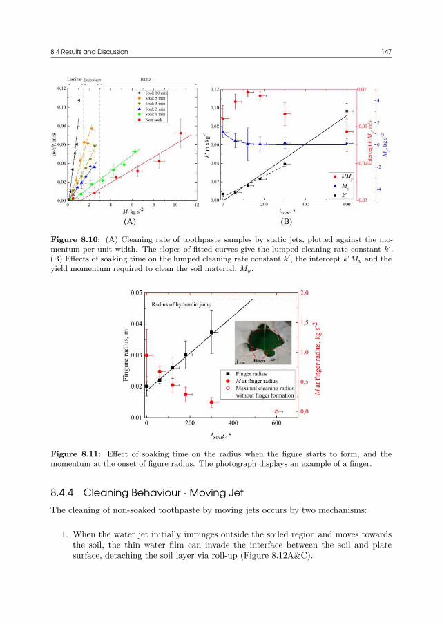
8.4 Results and Discussion 147
Figure 8.10: (A) Cleaning rate of toothpaste samples by static jets, plotted against the mo-mentum per unit width. The slopes of fitted curves give the lumped cleaning rate constant k′.(B) Effects of soaking time on the lumped cleaning rate constant k′, the intercept k′My and theyield momentum required to clean the soil material, My.
Figure 8.11: Effect of soaking time on the radius when the figure starts to form, and themomentum at the onset of figure radius. The photograph displays an example of a finger.
8.4.4 Cleaning Behaviour - Moving JetThe cleaning of non-soaked toothpaste by moving jets occurs by two mechanisms:
1. When the water jet initially impinges outside the soiled region and moves towardsthe soil, the thin water film can invade the interface between the soil and platesurface, detaching the soil layer via roll-up (Figure 8.12A&C).
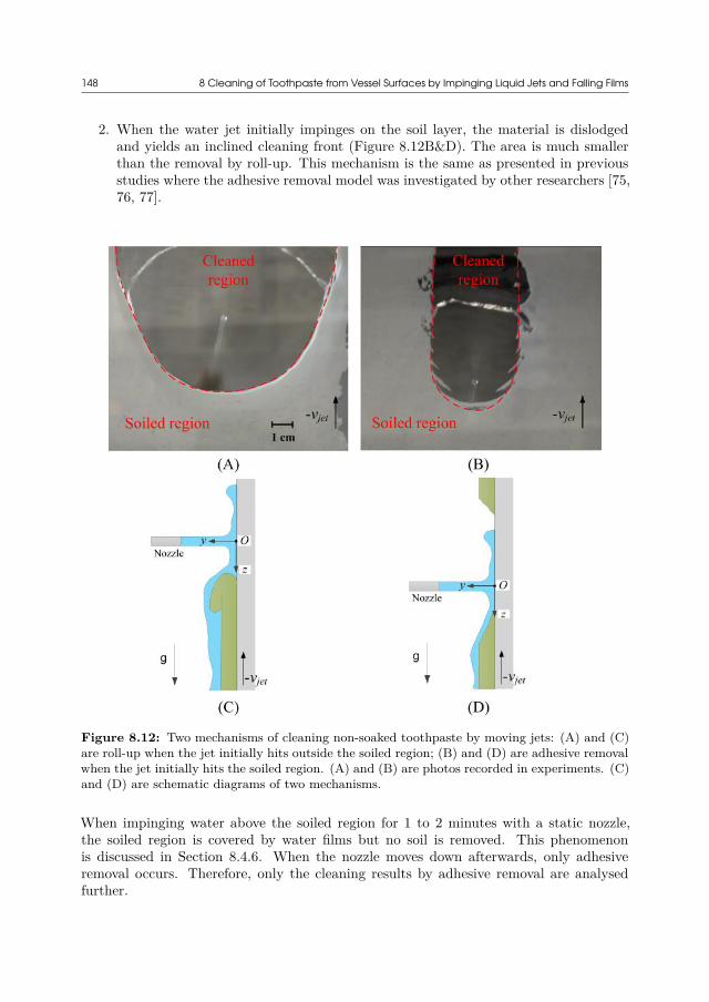
148 8 Cleaning of Toothpaste from Vessel Surfaces by Impinging Liquid Jets and Falling Films
2. When the water jet initially impinges on the soil layer, the material is dislodgedand yields an inclined cleaning front (Figure 8.12B&D). The area is much smallerthan the removal by roll-up. This mechanism is the same as presented in previousstudies where the adhesive removal model was investigated by other researchers [75,76, 77].
Figure 8.12: Two mechanisms of cleaning non-soaked toothpaste by moving jets: (A) and (C)are roll-up when the jet initially hits outside the soiled region; (B) and (D) are adhesive removalwhen the jet initially hits the soiled region. (A) and (B) are photos recorded in experiments. (C)and (D) are schematic diagrams of two mechanisms.
When impinging water above the soiled region for 1 to 2 minutes with a static nozzle,the soiled region is covered by water films but no soil is removed. This phenomenonis discussed in Section 8.4.6. When the nozzle moves down afterwards, only adhesiveremoval occurs. Therefore, only the cleaning results by adhesive removal are analysedfurther.
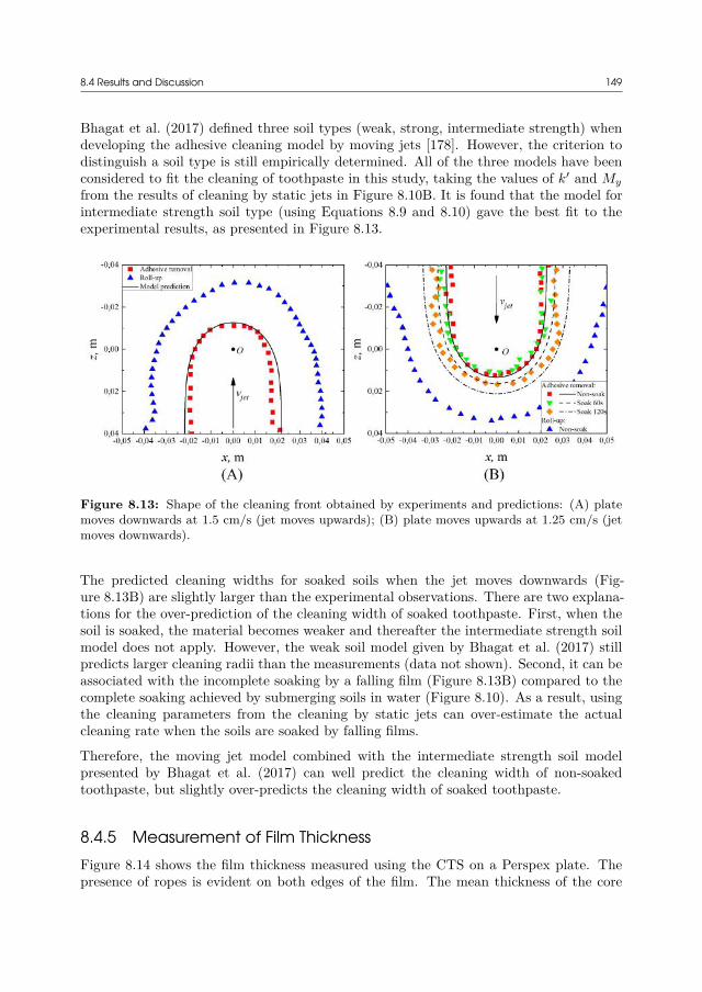
8.4 Results and Discussion 149
Bhagat et al. (2017) defined three soil types (weak, strong, intermediate strength) whendeveloping the adhesive cleaning model by moving jets [178]. However, the criterion todistinguish a soil type is still empirically determined. All of the three models have beenconsidered to fit the cleaning of toothpaste in this study, taking the values of k′ and My
from the results of cleaning by static jets in Figure 8.10B. It is found that the model forintermediate strength soil type (using Equations 8.9 and 8.10) gave the best fit to theexperimental results, as presented in Figure 8.13.
Figure 8.13: Shape of the cleaning front obtained by experiments and predictions: (A) platemoves downwards at 1.5 cm/s (jet moves upwards); (B) plate moves upwards at 1.25 cm/s (jetmoves downwards).
The predicted cleaning widths for soaked soils when the jet moves downwards (Fig-ure 8.13B) are slightly larger than the experimental observations. There are two explana-tions for the over-prediction of the cleaning width of soaked toothpaste. First, when thesoil is soaked, the material becomes weaker and thereafter the intermediate strength soilmodel does not apply. However, the weak soil model given by Bhagat et al. (2017) stillpredicts larger cleaning radii than the measurements (data not shown). Second, it can beassociated with the incomplete soaking by a falling film (Figure 8.13B) compared to thecomplete soaking achieved by submerging soils in water (Figure 8.10). As a result, usingthe cleaning parameters from the cleaning by static jets can over-estimate the actualcleaning rate when the soils are soaked by falling films.
Therefore, the moving jet model combined with the intermediate strength soil modelpresented by Bhagat et al. (2017) can well predict the cleaning width of non-soakedtoothpaste, but slightly over-predicts the cleaning width of soaked toothpaste.
8.4.5 Measurement of Film ThicknessFigure 8.14 shows the film thickness measured using the CTS on a Perspex plate. Thepresence of ropes is evident on both edges of the film. The mean thickness of the core
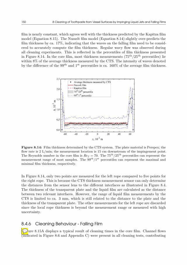
150 8 Cleaning of Toothpaste from Vessel Surfaces by Impinging Liquid Jets and Falling Films
film is nearly constant, which agrees well with the thickness predicted by the Kapitza filmmodel (Equation 8.15). The Nusselt film model (Equation 8.14) slightly over-predicts thefilm thickness by ca. 17%, indicating that the waves on the falling film need to be consid-ered to accurately compute the film thickness. Regular wavy flow was observed duringall cleaning experiments. This is reflected in the percentiles of film thickness presentedin Figure 8.14. In the core film, most thickness measurements (75th/25th percentiles) liewithin 8% of the average thickness measured by the CTS. The intensity of waves denotedby the difference of the 99th and 1st percentiles is ca. 160% of the average film thickness.
Figure 8.14: Film thickness determined by the CTS system. The plate material is Perspex; theflow rate is 2 L/min; the measurement location is 15 cm downstream of the impingement point.The Reynolds number in the core film is Ref = 70. The 75th/25th percentiles can represent themeasurement range of most samples. The 99th/1st percentiles can represent the maximal andminimal film thickness, respectively.
In Figure 8.14, only two points are measured for the left rope compared to five points forthe right rope. This is because the CTS thickness measurement sensor can only determinethe distances from the sensor lens to the different interfaces as illustrated in Figure 8.4.The thickness of the transparent plate and the liquid film are calculated as the distancebetween two relevant interfaces. However, the range of liquid film measurements by theCTS is limited to ca. 3 mm, which is still related to the distance to the plate and thethickness of the transparent plate. The other measurements for the left rope are discardedsince the local rope thickness is beyond the measurement range or measured with highuncertainty.
8.4.6 Cleaning Behaviour - Falling FilmFigure 8.15A displays a typical result of cleaning times in the core film. Channel flows
(indicated in Figure 8.6 and Appendix C) were present in all cleaning tests, contributing
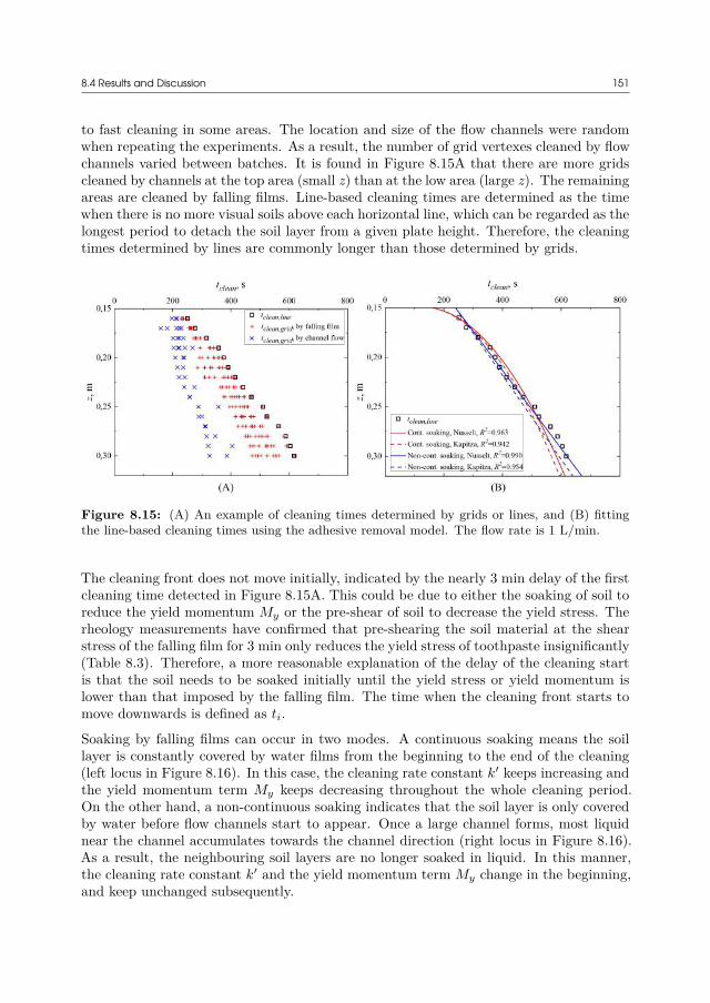
8.4 Results and Discussion 151
to fast cleaning in some areas. The location and size of the flow channels were randomwhen repeating the experiments. As a result, the number of grid vertexes cleaned by flowchannels varied between batches. It is found in Figure 8.15A that there are more gridscleaned by channels at the top area (small z) than at the low area (large z). The remainingareas are cleaned by falling films. Line-based cleaning times are determined as the timewhen there is no more visual soils above each horizontal line, which can be regarded as thelongest period to detach the soil layer from a given plate height. Therefore, the cleaningtimes determined by lines are commonly longer than those determined by grids.
Figure 8.15: (A) An example of cleaning times determined by grids or lines, and (B) fittingthe line-based cleaning times using the adhesive removal model. The flow rate is 1 L/min.
The cleaning front does not move initially, indicated by the nearly 3 min delay of the firstcleaning time detected in Figure 8.15A. This could be due to either the soaking of soil toreduce the yield momentum My or the pre-shear of soil to decrease the yield stress. Therheology measurements have confirmed that pre-shearing the soil material at the shearstress of the falling film for 3 min only reduces the yield stress of toothpaste insignificantly(Table 8.3). Therefore, a more reasonable explanation of the delay of the cleaning startis that the soil needs to be soaked initially until the yield stress or yield momentum islower than that imposed by the falling film. The time when the cleaning front starts tomove downwards is defined as ti.
Soaking by falling films can occur in two modes. A continuous soaking means the soillayer is constantly covered by water films from the beginning to the end of the cleaning(left locus in Figure 8.16). In this case, the cleaning rate constant k′ keeps increasing andthe yield momentum term My keeps decreasing throughout the whole cleaning period.On the other hand, a non-continuous soaking indicates that the soil layer is only coveredby water before flow channels start to appear. Once a large channel forms, most liquidnear the channel accumulates towards the channel direction (right locus in Figure 8.16).As a result, the neighbouring soil layers are no longer soaked in liquid. In this manner,the cleaning rate constant k′ and the yield momentum term My change in the beginning,and keep unchanged subsequently.
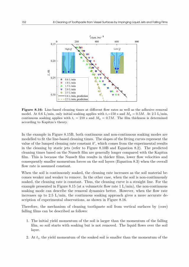
152 8 Cleaning of Toothpaste from Vessel Surfaces by Impinging Liquid Jets and Falling Films
Figure 8.16: Line-based cleaning times at different flow rates as well as the adhesive removalmodel. At 0.6 L/min, only initial soaking applies with ti=150 s and My = 0.5M . At 2.5 L/min,continuous soaking applies with ti = 210 s and My = 0.7M . The film thickness is determinedaccording to Kapitza’s theory.
In the example in Figure 8.15B, both continuous and non-continuous soaking modes aremodelled to fit the line-based cleaning times. The slopes of the fitting curves represent thevalue of the lumped cleaning rate constant k′, which comes from the experimental resultsin the cleaning by static jets (refer to Figure 8.10B and Equation 8.2). The predictedcleaning times based on the Nusselt film are generally longer compared with the Kapitzafilm. This is because the Nusselt film results in thicker films, lower flow velocities andconsequently smaller momentum forces on the soil layers (Equation 8.3) when the overallflow rate is assumed constant.
When the soil is continuously soaked, the cleaning rate increases as the soil material be-comes weaker and weaker to remove. In the other case, when the soil is non-continuouslysoaked, the cleaning rate is constant. Thus, the cleaning curve is a straight line. For theexample presented in Figure 8.15 (at a volumetric flow rate 1 L/min), the non-continuoussoaking mode can describe the removal dynamics better. However, when the flow rateincreases up to 2.5 L/min, the continuous soaking approach gives a more accurate de-scription of experimental observations, as shown in Figure 8.16.
Therefore, the mechanism of cleaning toothpaste soil from vertical surfaces by (core)falling films can be described as follows:
1. The initial yield momentum of the soil is larger than the momentum of the fallingfilm, so soil starts with soaking but is not removed. The liquid flows over the soillayer.
2. At ti, the yield momentum of the soaked soil is smaller than the momentum of the

8.4 Results and Discussion 153
falling film. The toothpaste soil starts to be removed by adhesive failure. Channelflow appears at the same time or earlier.
3. At low flow rates, all liquid flows down through channels, so only the cleaning frontand channel boundaries are contacted with liquid. The rest of the soil layer is notfurther soaked. Therefore, the cleaning front moves down at a constant rate.
4. At high flow rates, a fraction of the liquid flows through the channels and theremainder flows over the soil layer. The liquid continues soaking the soil and thecleaning rate keeps increasing.
Flow channels are formed when the liquid film tears a small gap of the soil layer and theneighbouring liquid accumulates toward the gap direction. As a result, the flow rate in theflow channel increases. According to Figure 8.16, the transition between non-continuoussoaking and continuous soaking occurs at a flow rate of 2 - 2.5 L/min, corresponding toa wetting rate Γcore = 0.097 - 0.112 kg/(m s). This critical range is much lower than thestandard by ASME BPE, which requires 0.517 - 0.617 kg/(m s) wetting rate for cleaningvertical cylindrical vessels with static spray devices [184].
One more cleaning test was performed with the whole plate covered by toothpaste (seeFigure 8.5D), in order to compare with the results where only the downstream plate issoiled and cleaned solely by a falling film. As shown in Figure 8.17, cleaning starts aroundthe impingement point immediately after the water jet touches the soil layer. The cleanedarea expands outwards and downwards. Flow channels with high flow rates can peel offthe neighbouring soil layers rapidly. The slowest cleaning region is regarded as adhesiveremoval where the developed model in this study applies. The boundary of the finalcleaned region indicates the footprint of the water film. The line-based cleaning time toclean to 30 cm downstream of the impingement point is around 550 s, in comparison with583 ± 22 s when the plate is only soiled at 15 - 30 cm downstream. Thus, the cleaningtimes determined from these two different initial soiling areas are very similar. The slightdifference can be caused by experimental deviations, since the position and size of theflow channels differ in every experiment.
To sum up, the momentums of water films are significantly different between the impinge-ment area (> 0.1 kg s-2) and the falling film (< 0.05 kg s-2). It has been shown thatthe adhesive model developed by Wilson et al. (2012) [72] and Bhagat et al. (2017) [178]for cleaning near the impingement region also applies to the cleaning by falling films.However, there are still some challenges to use the model to the cleaning of toothpaste byfalling films: firstly, the value of the yield momentum of toothpaste after soaking is highlyuncertain, which requires a more accurate method for exact determination; secondly, thesoaking mechanism of toothpaste by falling films differs from that by submerging soils inwater, which leads to great deviations when taking the model parameters from the clean-ing by static jets to the cleaning by falling films; thirdly, the initial delay of the cleaningfront moving down is caused by the soaking of soil, the period of which is related to theflow conditions but the detailed mechanism behind this is not completely understood yet.
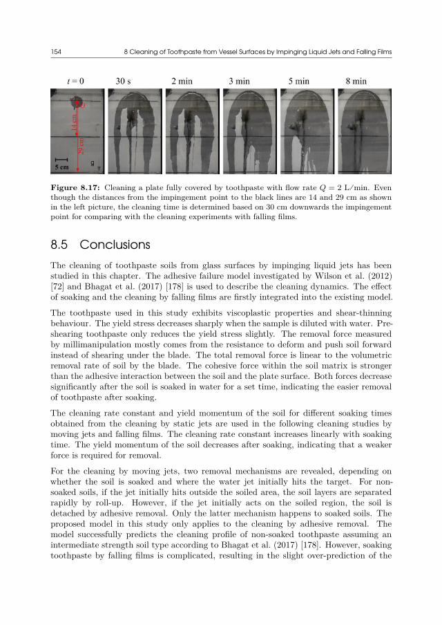
154 8 Cleaning of Toothpaste from Vessel Surfaces by Impinging Liquid Jets and Falling Films
Figure 8.17: Cleaning a plate fully covered by toothpaste with flow rate Q = 2 L⁄min. Eventhough the distances from the impingement point to the black lines are 14 and 29 cm as shownin the left picture, the cleaning time is determined based on 30 cm downwards the impingementpoint for comparing with the cleaning experiments with falling films.
8.5 ConclusionsThe cleaning of toothpaste soils from glass surfaces by impinging liquid jets has beenstudied in this chapter. The adhesive failure model investigated by Wilson et al. (2012)[72] and Bhagat et al. (2017) [178] is used to describe the cleaning dynamics. The effectof soaking and the cleaning by falling films are firstly integrated into the existing model.
The toothpaste used in this study exhibits viscoplastic properties and shear-thinningbehaviour. The yield stress decreases sharply when the sample is diluted with water. Pre-shearing toothpaste only reduces the yield stress slightly. The removal force measuredby millimanipulation mostly comes from the resistance to deform and push soil forwardinstead of shearing under the blade. The total removal force is linear to the volumetricremoval rate of soil by the blade. The cohesive force within the soil matrix is strongerthan the adhesive interaction between the soil and the plate surface. Both forces decreasesignificantly after the soil is soaked in water for a set time, indicating the easier removalof toothpaste after soaking.
The cleaning rate constant and yield momentum of the soil for different soaking timesobtained from the cleaning by static jets are used in the following cleaning studies bymoving jets and falling films. The cleaning rate constant increases linearly with soakingtime. The yield momentum of the soil decreases after soaking, indicating that a weakerforce is required for removal.
For the cleaning by moving jets, two removal mechanisms are revealed, depending onwhether the soil is soaked and where the water jet initially hits the target. For non-soaked soils, if the jet initially hits outside the soiled area, the soil layers are separatedrapidly by roll-up. However, if the jet initially acts on the soiled region, the soil isdetached by adhesive removal. Only the latter mechanism happens to soaked soils. Theproposed model in this study only applies to the cleaning by adhesive removal. Themodel successfully predicts the cleaning profile of non-soaked toothpaste assuming anintermediate strength soil type according to Bhagat et al. (2017) [178]. However, soakingtoothpaste by falling films is complicated, resulting in the slight over-prediction of the
8.5 Conclusions 155
cleaning width according to the model.
The adhesive model developed from the cleaning around the impingement point canalso apply to the cleaning by falling films. Kapitza’s theory results in a more accurateprediction of the falling film thickness because of the presence of wavy flow. The existenceof flow channels can speed up the removal of some local areas. But the removal rate inthe hardest removal area can be predicted by the adhesive model. It takes a period forthe cleaning front to start moving down since the soil needs to be soaked until the yieldmomentum is less than the flow momentum. At low flow rates (less than 0.097 - 0.112kg/(m s) wetting rate of core film), the soaking effect terminates when the cleaning frontmoves down or large flow channels form, as most liquid accumulates towards the flowchannels and the soil layer is no longer exposed to a water film. On the other hand, whenthe flow rate is above the transition wetting rate, a continuous soaking effect works on thesoil layer until cleaning ends. The line-based cleaning time resulted from the plate thatis fully covered by soil is close to the cleaning time when only soiling the area below theimpingement point. In the present model, some challenges should be resolved for moreaccurate prediction of cleaning by falling films, including the determination of the yieldmomentum after soaking, the mechanism of toothpaste soaking by falling films, and theinitial delay of the cleaning front moving down.
List of Nomenclature in Chapter 8The following nomenclature is only valid for this chapter. Some symbols are used in otherchapters but with different meanings. Otherwise, the symbols are specifically explainedin the text if there is no nomenclature in some chapter.
Roman Lettersa Cleaning distance, [m]aX Distance to cleaning front on moving jet path, [m]A Cleaning rate parameter defined by A = 1 − 10πµr0/3m, dimen-
sionlessAblade Area of millimanipulation blade tip, [m2]B Cleaning rate parameter defined by B = 10πµ/3mr2
0, dimension-less
C1 Constant defined by C1 =∫ 1
0 f(η)2dη, dimensionlessC2 Constant defined by C2 =
∫ 10 f(η)dη, dimensionless
d Jet diameter, [m]fc Fraction of flow in core film, dimensionlessFW Force per unit width measured by millimanipulation, [N m-1]FW, normal Normal force per unit width, [N m-1]FW, shear Shear force per unit width, [N m-1]g Gravitational acceleration, [m s-2]G′ Elastic modulus, [Pa]G′′ Viscous modulus, [Pa]h Film thickness, [m]
156 8 Cleaning of Toothpaste from Vessel Surfaces by Impinging Liquid Jets and Falling Films
hKapitza Mean film thickness based on Kapitza’s theory, [m]hNusselt Mean film thickness based on Nusselt’s theory, [m]k0 Lumped cleaning rate constant without soaking, [m s kg-1]k1 Lumped cleaning rate constant per soaking time, [m kg-1]k′ Lumped cleaning rate constant, [m s kg-1]Lblade Length of the millimanipulation contacting with soil, [m]m Mass flow rate, [kg s-1]M Momentum per unit width, [kg s-2]My Yield momentum per unit width of material, [kg s-2]p Radial distance to cleaning front, [m]p∗ Dimensionless radial distance to cleaning front, dimensionlessq Volumetric flow rate per unit width, [m2 s-1]Q Volumetric flow rate, [m3 s-1]r Radial coordinate, [m]r0 Nozzle radius, [m]rb Radius where boundary layer reaches the surface, [m]rt Transition radius from laminar to turbulent flow, [m]R Radius of impingement region, [m]Ref Film Reynolds number defined by Ref = 4ρq/µ, dimensionlessRej Jet Reynolds number, dimensionlesst Time, [s]tclean, grid Cleaning time based on grid, [s]tclean, line Cleaning time based on line, [s]tsoak Soaking time, [s]u Flow velocity, [m s-1]U0 Mean flow velocity from jet, [m s-1]Uav Mean flow velocity, [m s-1]Us Surface flow velocity, [m s-1]vblade Millimanipulation blade velocity, [m s-1]vjet Jet velocity, [m s-1]W Falling film width, [m]Wblade Width of the millimanipulation blade, [m]Wc Core film width, [m]x, y, z Coordinates, [m]
Greek Lettersβ Angle to direction of nozzle motion, dimensionlessγ Surface tension (liquid/vapour), [N m-1]γ Apparent shear rate, [s-1]δ Boundary layer thickness, [m]δsoil Soil thickness, [m]δgap Gap distance of millimanipulation blade, [m]η Distance normal to the wall defined by η = y/δ, dimensionlessηapp Apparent viscosity, [Pa s]θ Contact angle, dimensionlessµ Dynamic viscosity, [Pa s]

8.5 Conclusions 157
ρ Density, [kg m-3]σ Cleaning rate parameter defined by σ = 3k′mU0/5π, [m2 s-1]τy Yield stress, [Pa]χ Phase angle, [°]Γ Wetting rate, [kg m-1 s-1]Γcore Wetting rate in core film, [kg m-1 s-1]Γrope Wetting rate in rope, [kg m-1 s-1]

158

Part III
Conclusions and Perspectives

CHAPTER9Overall Conclusions
The primary topic of this Ph.D work was to investigate different approaches for reducingresource consumption and cleaning costs during CIP operations. In the mapping studyin a brewery, it was shown that most of the cleaning time and the main cleaning costs arespent on the cleaning detergent steps. The recovery of cleaning detergents can reduce thecleaning costs significantly. The annual cleaning costs for pipes are higher than the costsof tank cleaning operations, because the former occurs more frequently than the latter.The main findings in the brewery and the suggestions for implementing best practice areuseful to improve the CIP systems in other industries where similar processes are used.
Analysing the historical data from the CIP of a brewery fermenter provides a benchmarkthat allows use of the historical cleaning data to improve the CIP operations in thefuture. In the presented case, a three-level analysis approach was used to evaluate a CIPsystem or operation to be normal or abnormal online or offline. Univariate analysis wasapplied in the first and third levels for assessing the CIP performance before and afterthe batch, respectively. Multivariate analysis was used in the second level of analysis tolocally indicate the occurrence of anomalous events. The implementation of the analysisapproach has significant potential to automatically detect the deviations and anomaliesin future CIP cycles and to optimize the cleaning process.
CFD is a powerful tool to simulate the displacement of cleaning agent by water in pipesystems during the intermediate and final rinse steps in the cleaning of pipes. Based onthe results from CFD simulations, it was found that dead zones mainly exist in the areaswhere flow recirculation is strong. The size of dead zones can be reduced by employingsmooth connections or large flow velocities, but the occurrence of dead zones cannotbe completely avoided. Increasing the flow velocity is able to reduce the rinsing time,but the overall water consumption is merely changed by varying flow velocity. In mostsituations, determining the rinsing time based on a local measurement is a safe wayto avoid contamination risks, but is not the most economic way to minimise the actualwater consumption. Furthermore, CFD supplements the traditional empirical approach tocompute the pressure drop and equivalent length of different pipe elements. Summarizing,the present study proves that CFD is a helpful tool to optimize the hygienic design ofpipe systems and to improve the cleaning efficiency.
Cleaning tank surfaces using pulsed flows has potentials to save cleaning costs. For thecleaning of tank surface soiled by egg yolk soil, pulsed flow is able to remove more depositsthan continuous flow at the same consumption of alkaline solution, but at the expense oflonger actual cleaning time. The enhancement of the cleaning effect by pulsed flow occurs

162 9 Overall Conclusions
primarily because additional time is provided for soil layers to swell. Then the materialsbecome easy to remove in the next pulse of flow. The most efficient burst technique ispulsing with high frequency and short period. Pre-wetting prior to continuous flow showsno significant improvement of the cleaning result. Cooking the soiling material above itsdenaturation temperature makes the soil more difficult to detach. For cleaning egg yolkby alkaline solution, the optimal cleaning conditions are high flow rate, high temperature(below denaturation temperature), and low alkali concentration. The main findings inpilot scale tests are also found in scale-up tests.
Common measurement-based CIP aims to control the cleaning time when there is nodetectable soil in the liquid phase. However, there is still a risk that inconspicuoustraces exist even though the measurement indicates a clear signal. Instead of extendingthe cleaning time using fresh water, a three-stage measurement-based partial recoveryapproach was designed with a turbidity sensor applied to measure the water quality.Reused water is utilised in the first stage to remove bulk soils and sent to drain directly.When the water is relatively clear, the circulation of reused water is started for a pre-defined period to detach all small traces from the surfaces. Fresh water is then used in thethird stage to remove all remaining dirt, and is then recycled for the next cleaning. In thismanner, the overall cleaning is performed for a sufficient period without increasing theconsumption of fresh water. The water volume in the reused water tank keeps unchanged.So the cleaning water can be reused several times. The lifetime of the reused cleaningwater can be prolonged by avoiding the accumulation of impurities in the reused watertank. The cleaning costs of the proposed three-stage measurement-based partial recoveryapproach yield the most economic scenario compared with single-use, full recovery, andtime-based partial recovery approaches.
The cleaning of toothpaste soils from glass surfaces by impinging liquid jets and fallingfilms can be predicted by the adhesive failure model investigated by Wilson et al. (2012)and Bhagat et al. (2017). This thesis is the first work to integrate the effect of soakingand the cleaning by falling films into the existing model. Toothpaste exhibits viscoplasticproperties and shear-thinning behaviour. The soil becomes easier to remove after dilutionor soaking. Pre-shearing the soil prior to cleaning is less important than soaking. Thecleaning rate constant and yield momentum of soil for different soaking times obtainedfrom the cleaning by static jets can be used in the cleaning studies by moving jets andfalling films. However, the mechanism of cleaning non-soaked toothpaste by moving jetsdepends on whether the soil is soaked and where the water jet initially hits the target,resulting in the removal by either roll-up or adhesive removal. Only the latter mechanismapplies to the removal of soaked soils. For the cleaning by falling films, Kapitza’s theoryresults in more accurate prediction of falling film thickness than Nusselt’ theory due tothe presence of wavy flow. At low flow rate, the soil is non-continuously soaked until thecleaning front moves down or large flow channels appear. When the flow rate is above thetransition wetting rate, a continuous soaking effect acts on the soil layer until cleaningends.
CHAPTER10Perspectives
The objective of this Ph.D work was to investigate the opportunities for improving CIPoperations, with particular focus on the CIP practices in brewery or similar industries.This chapter consists of two sections: the first summarizes the suggestions of future workbased on the studies in Chapters 4 to 8; the second section provides other state-of-the-arttechniques to improve the performance of CIP operations in industrial applications.
10.1 Suggestions for Future WorkChapters 4 to 8 present independent case studies. The future work suggested in thissection is also organised by chapter:
1. The three-level analysis approach in Chapter 4 can be applied to other CIP sys-tems than the cleaning of brewery fermenters. With more data integrated into theproposed model, particularly water quality measurement, it should be possible topredict the end point of cleaning. Furthermore, the present study only indicatesthe occurrence of anomalies in a cleaning process and the likely causes. A detailedtrouble-shooting approach is required to diagnose the root cause of an anomaly.
2. Part of the simulations of pipe cleaning and rinsing using CFD (Chapter 5) hasbeen validated using analytical approaches and experimental results available inthe literature. More experiments are needed to compare with the simulations ofvarious pipe elements. Considering the numerous combinations of geometries, sizesand flow conditions, etc., a more practical solution is to focus on an existing pipesystem and identify the most difficult cleaning part for analysis.
3. The enhancement of cleaning by pulsed flow was examined by cleaning egg yolksoils by alkaline solutions in Chapter 6. Egg yolk is a complicated soil type becauseof its denaturation property at high alkaline concentration and at high temperature.Therefore, a more simple soil type could be useful for further investigations of bursttechniques in tank cleaning. Besides, the burst parameters (e.g., frequency, ratio ofeffective and holding times) can be optimized for removing more deposits per unitcost of cleaning resources.
4. The measurement-based partial recovery CIP system presented in Chapter 7 onlyuses water as cleaning medium. Similar approaches can be applied to other cleaningsteps where chemicals are utilised. The lifetime of the cleaning liquid depends on
164 10 Perspectives
various factors like the type of deposits to be cleaned and quality requirement.Therefore, the determination of liquid lifetime is another important characteristicfor evaluating the cost saving in CIP recovery processes.
5. The flow rates of liquid jets (indicated by the wetting rate of liquid film) in Chapter 8are much lower than the recommendation for cleaning large tank vessels by theASME BPE standard. Therefore, some phenomena (i.e., non-continuous soaking byfalling films) may not occur after scaling up. It is worth investigating the differentsoaking approaches of toothpaste described in Chapter 8, such as dilution withwater, submersing under water, soaking by falling films.
10.2 Other Opportunities for Improving Industrial CIPOperations
10.2.1 Smart Scheduling of Production and CleaningCleaning has often been regarded as a supplementary activity executed after presentproduction or before a new production. As a result, plenty of studies have focused onhow to improve the productivity instead of how to save costs from cleaning, even thoughpeople universally agree that magnificent resource savings can be achieved through theefficient implementation of CIP. In fact, the cleaning costs can be hugely decreased, orat least avoid being wasted, by smartly scheduling production and cleaning plans. Forinstance:
• Immediate cleaning after production can avoid the formation of hard-to-clean soils.Soil materials become more difficult to clean after a long holding period because ofsoil drying, reaction and microbial growth, etc. Therefore, soils should be cleanedimmediately after production to avoid unnecessary waste of cleaning resources.
• Avoiding long waiting time between two production batches can reduce unnecessaryrepeated cleaning cycles. Once some equipment is held for long time, for exampletwo weeks for brewery fermenters, it is required to conduct cleaning before usage.A smart scheduling of production and facility utilisation should avoid this kind oflong holding time and therewith needless cleaning.
• Identical or similar products can be allocated for production together. When thesame or similar products are produced by the same facility, cleaning can be avoidedor performed after a number of batches. It is also possible to execute a shortcleaning recipe between alteration instead of long and expensive recipes, which cansave cleaning costs significantly.
• Low-contaminated production can be planned prior to high-contaminated produc-tion. In such a manner, the cleaning between two production batches can be per-formed using a simple recipe. A good example is that when producing normal cola
10.2 Other Opportunities for Improving Industrial CIP Operations 165
and sugar-free cola, a fast cleaning is needed when producing sugar-free before nor-mal cola, in comparison to a complex cleaning recipe when planning normal colaahead of sugar-free cola.
10.2.2 Membrane TechnologyMembrane processes have become an integral part of food processing, and are used toseparate a liquid feed stream into two separate streams, namely permeate and retentate.This separation is mainly driven by the pressure difference across the membrane. As thefiltration continues, the membrane and pores are gradually filled with feed componentswith high solid level, which consequently decreases the separation efficiency. Therefore,the cleaning of membranes have become more and more important in order to restoreproduction capacity [6], especially for the reverse osmosis (RO) elements with small holes.This cleaning is commonly done by CIP with various types of cleaning agent such as caus-tic, acid, proteolytic enzymes and proprietary additives (surfactants and sequestrants),due to the complex matrix of fouling layers. The cleaning of membrane systems is recom-mended to be performed separately from other equipment to avoid inter-contamination.Trans-membrane pressure (TMP) is one of the key characteristics to assess membranefouling and cleaning.
Another application of membrane systems is to treat waste water and water for reuseby recovering cleaning detergent compounds from CIP processes [185, 186, 187]. Forexample, Suárez et al. (2015) used a nanofiltration pilot plant to recover the CIP solutionin an industrial yoghurt factory. Membranes retained nearly 90% of the chemical oxygendemand (COD). The permeates could be reused in the CIP plant without reducing thecleaning efficiency. The fresh detergent savings were around 18% [61]. Another study byDresch et al. (2001) compared the continuous and discontinuous approaches to integratea nanofiltration system in a CIP process to recover alkaline solution in the dairy industry.Whatever the selected integrated process, the COD level in the CIP tank stabilized at alevel depending on the membrane area, which, however, was much lower than the CODcontent in commonly recycled CIP systems without membrane regeneration [188].
10.2.3 Novel Cleaning Agents
10.2.3.1 Enzyme-Based Cleaner
Enzymatic cleaning is advantageous to the environment because less aggressive conditionsare required and a lower amount of salt is released compared to the traditional alkalitreatment [189]. In a recent study, a 2-stage CIP operation was investigated by Chutrakulet al. (2018) to soak coconut milk fouling. Using surfactant linear alkylbenzene sulfonates(stage 1) prior to cellulase treatment (stage 2) could remove the foulants to a similar extentcompared with only using NaOH solution for the same soaking time. The enzymaticapproach is superior to the alkaline approach because of the lower temperature and lowerpH required by the enzyme, and the biodegradability of surfactant and cellulase [190].
166 10 Perspectives
10.2.3.2 Electrolysed Water
Electrolysed water is an effective cleaning and sanitizing agent. Compared with conven-tional chemical sanitizers, electrolysed water has the advantages of low risk to produceand little addition of toxic heavy metals. Electrolysed water can be generated by theelectrolysis of a dilute NaCl solution using two electrodes. Traditionally, the cathode andanode electrodes are separated by membranes. In the anode cell, water reacts with theanode electrode, producing oxygen and hydrogen ions. Chlorine ions can also react withthe electrode, generating chlorine gas and hypochlorous acid (HOCl). This solution iscalled acidic electrolysed water with a pH value of 2.7 or lower. Acidic electrolysed wateris able to inactivate a variety of bacterial pathogens on the surfaces of food processingequipment [136]. Compared with traditional chlorine-based solutions, electrolysed wateris more effective in killing microbes, hence, lower concentration is required. Novel tech-nology allows to generate electrolysed water without using a membrane to separate thecathode and anode electrodes. Thereby, neutral electrolysed water is produced with lowrisk of corrosion of processing equipment and low irritation to operators [191].
10.2.4 Pigging TechnologyPushing a piston through a pipe, commonly known as pigging, is an efficient techniqueto recover the product from a pipeline and clean the pipe wall. Conventionally, solid pigswith simple geometries are propelled by compressed air, water or another liquid throughthe pipes with a uniform diameter. Clever mechanical design and the use of compliantmaterials have extended the application of pigging to the pipelines with minor geometrychanges. However, there are still barriers when installing a pigging system to an existingproduction line, due to the existence of valves, sensors, heat exchangers, pumps, etc.
An innovative method of pigging is to use crushed ice rather than a solid to removeviscous products and fouling. According to Quarini (2002), a mixture of ice particles andwater with a freezing point depressant is pumped through various geometries, includingstraight pipes, bends, T-joints, static mixers, orifices and plate heat exchangers, etc.The ice-pigging technique can never get stuck even at the most complex heat exchangergeometry. The use of water has considerable environmental benefits [192, 193]. However,The biggest challenge to limit the application of ice-pigging is the high costs to make andstore ice [59].

Part IV
Appendices

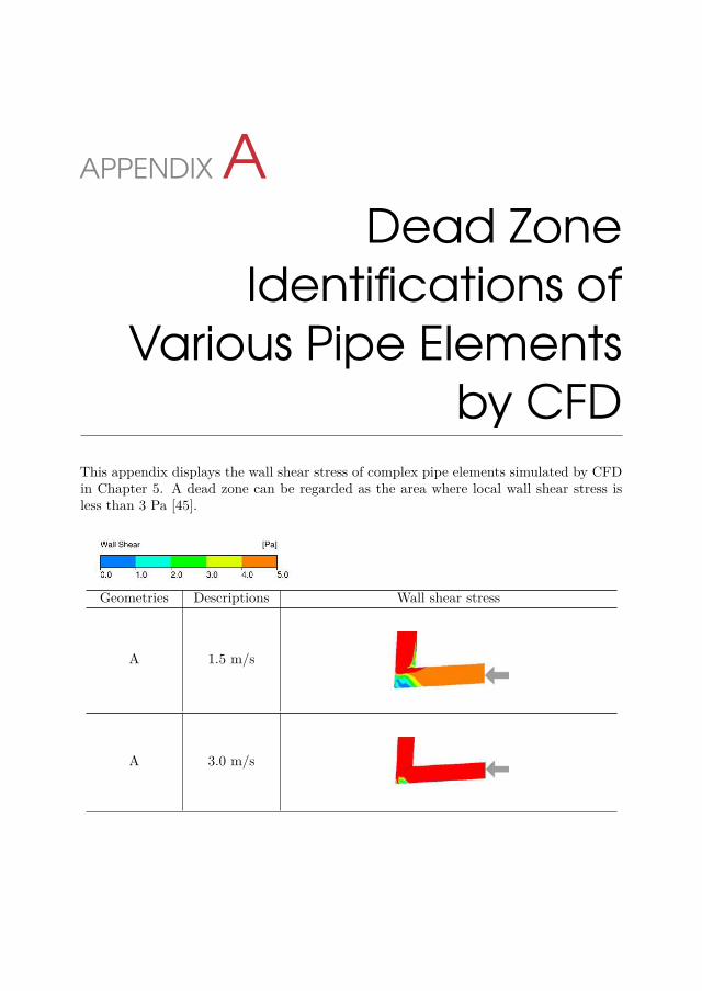
APPENDIXADead Zone
Identifications ofVarious Pipe Elements
by CFDThis appendix displays the wall shear stress of complex pipe elements simulated by CFDin Chapter 5. A dead zone can be regarded as the area where local wall shear stress isless than 3 Pa [45].
Geometries Descriptions Wall shear stress
A 1.5 m/s
A 3.0 m/s

170 A Dead Zone Identifications of Various Pipe Elements by CFD
B 1.5 m/s
B 3.0 m/s
C 1.5 m/s
C 3.0 m/s
D 1.5 m/s
D 3.0 m/s
E 1.5 m/s
F 1.5 m/s
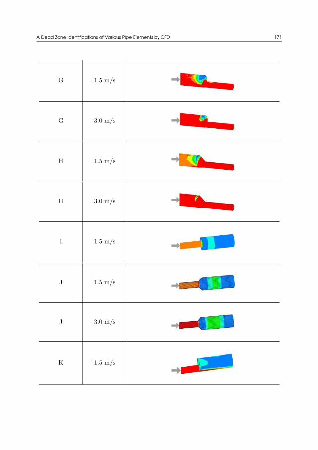
A Dead Zone Identifications of Various Pipe Elements by CFD 171
G 1.5 m/s
G 3.0 m/s
H 1.5 m/s
H 3.0 m/s
I 1.5 m/s
J 1.5 m/s
J 3.0 m/s
K 1.5 m/s

172 A Dead Zone Identifications of Various Pipe Elements by CFD
L 1.5 m/s
M 1.5 m/s
N 1.5 m/s
O 1.5 m/s
P
1.5 m/s,views from
twoperspectives
APPENDIXBCleaning Dynamics ofEgg Yolk Soils from Tank
Surfaces (All Data)This appendix is an extension of Figure 6.4 in Chapter 6, showing the removal of uncookedegg yolk soils from tank surfaces under all experimental conditions.

174 B Cleaning Dynamics of Egg Yolk Soils from Tank Surfaces (All Data)
Figure B.1: Removal of uncooked soils for all runs under different conditions of temperature,flow rate and NaOH concentration, by using continuous flow without pre-wetting (C1) or pulsedflow in short period and high frequency (P1): (A) tank upper wall, (B) tank middle wall, (C)tank lower wall, (D) tank overall wall surface.

APPENDIXCThe Development of
Flow Channels Duringthe Cleaning of
Toothpaste by FallingFilms
This appendix displays the development of flow channels during the cleaning of toothpasteby falling films in Chapter 8. Flow channels appear spontaneously in all experiments withflow rate ranging from 0.6 - 2.5 L/min. In the flow channel region, the soiled materialis removed slower than by a rope but faster than by a falling film. Flow channels formbefore the cleaning front starts to move.

176 C The Development of Flow Channels During the Cleaning of Toothpaste by Falling Films
Figure C.1: The development of flow channels during the cleaning of toothpaste by fallingfilms. The example is at flow rate 2 L/min, the same condition as in Figure 8.6. (A) Cleaningstarts. (B) Flow channel starts to form, but the cleaning front does not move. (C) Flow channelgrows, but the cleaning front does not move. (D) More flow channels form, and the cleaningfront starts to move. (E) More flow channels grow, and the cleaning front moves fast. (E) Moreareas are cleaned.

List of PublicationsPeer-reviewed manuscripts
Yang, J., Jensen, B. B. B., Nordkvist, M., Rasmussen, P., Pedersen, B., Kokholm, A.,Jensen, L., Gernaey, K. V., Krühne, U. (2018). Anomaly Analysis in Cleaning-in-PlaceOperations of an Industrial Brewery Fermenter. Industrial and Engineering ChemistryResearch, 57 (38): 12871 - 12883.DOI: 10.1021/acs.iecr.8b02417
Yang, J., Jensen, B. B. B., Nordkvist, M., Rasmussen, P., Gernaey, K. V., Krühne, U.(2018). CFD modelling of axial mixing in the intermediate and final rinses of cleaning-in-place procedures of straight pipes. Journal of Food Engineering, 221: 95 - 105.DOI: 10.1016/j.jfoodeng.2017.09.017
Yang, J., Kjellberg, K., Jensen, B. B. B., Nordkvist, M., Gernaey, K. V., Krühne, U.(2018). Investigation of the cleaning of egg yolk deposits from tank surfaces using con-tinuous and pulsed flows. Food and Bioproducts Processing, in press.DOI: 10.1016/j.fbp.2018.10.007
Conference proceedings and abstracts
Yang, J., Kjellberg, K., Jensen, B.B.B., Nordkvist, M., Gernaey, K.V., Krühne U. (2018).Cleaning of tank surfaces fouled by egg yolk. 17 – 20 April 2018, Fouling and Clean-ing in Food Processing Conference, Lund, Sweden. Accepted for oral presentation andproceeding publication.
Yang, J., Gernaey, K., Krühne, U., Rasmussen, P., Kokholm, A., Nordkvist, M. (2018).Industrial cleaning-in-place processes in brewery – a systematic mapping study. 30 Jan-uary 2018, 12th Annual Water Research Meeting of Danish Water Forum, Copenhagen,Denmark. Accepted for oral presentation and abstract publication.
Yang, J., Nordkvist, M., Gernaey, K. V., Krühne, U. (2017). Anomaly Detection and Di-agnosis Using Multivariate Analysis Tools in Industrial Cleaning-in-Place Operations. 12– 14 June 2017, IChemE Advances in Process Automation and Control 2017, Birmingham,UK. Accepted for oral presentation.
Yang, J., Gernaey, K. V., Krühne, U. (2016). Simulation of Axial Mixing by CFD duringthe Rinse of CIP procedures. 2 - 3 Nov. 2016, EHEDG World Congress on HygienicEngineering and Design 2016, Herning, Denmark. Accepted for poster presentation andproceeding publication.

178

Bibliography[1] I Palabiyik et al. “Minimising the environmental footprint of industrial-scaled
cleaning processes by optimisation of a novel clean-in-place system protocol”. In:Journal of Cleaner Production 108 (2015), pages 1009–1018.
[2] TR Bott. Fouling notebook. Institution of Chemical Engineers, 1990.[3] L Melo, TR Bott, and CA Bernardo. Fouling science and technology. Volume 145.
Springer Science & Business Media, 2012.[4] B Jude and E Lemaire. “How to optimize clean-in-place (cip) processes in food
and beverage operations”. In: Scheider Electric (2013).[5] DA Seiberling. Clean-in-place for biopharmaceutical processes. CRC Press, 2007.[6] AY Tamime. Cleaning-in-Place: dairy, food and beverage operations. 3rd edition.
Ayr, UK: Blackwell, 2008, page 272.[7] EHEDG Secretariat. EHEDG Yearbook 2016/2017. 2017.[8] JE Frantsen and TE Mathiesen. “Specifying stainless steel surfaces for the brewery,
dairy and pharmaceutical sectors”. In: Corrosion 2009 (2009).[9] HLM Lelieveld, MA Mostert, and J Holah. Handbook of hygiene control in the food
industry. 1st edition. Cambridge, UK: Woodhead Publishing, 2005, page 744.[10] DW Sun. Computational fluid dynamics in food processing. CRC Press, 2007.[11] Erwin, AP and A Graßhoff. “Cleaning and Sanitation”. In: Handbook of Food
Engineering. Edited by DR Heldman and DB Lund. Second Edi. CRC Press, 2006.Chapter 14, pages 929–975.
[12] PJ Fryer, GK Christian, and W Liu. “How hygiene happens: physics and chemistryof cleaning”. In: International Journal of Dairy Technology 59.2 (2006), pages 76–84.
[13] I Palabiyik. “Investigation of fluid mechanical removal in the cleaning process”.PhD thesis. University of Birmingham, 2013.
[14] B Van der Bruggen and L Braeken. “The challenge of zero discharge: from waterbalance to regeneration”. In: Desalination 188.1-3 (2006), pages 177–183.
[15] PJ Fryer and K Asteriadou. “A prototype cleaning map: a classification of indus-trial cleaning processes”. In: Trends in Food Science & Technology 20.6-7 (2009),pages 255–262.
180 Bibliography
[16] MR Bird and PJ Fryer. “Experimental study of the cleaning of surfaces fouled bywhey proteins”. In: Food and Bioproducts Processing 69.1 (1991), pages 13–21.
[17] MR Bird and PJ Fryer. “An analytical model for the cleaning of food process plant”.In: Food Engineering in a Computer Climate. Taylor & Francis. 1992, pages 325–330.
[18] N Akhtar et al. “Matching the nano-to the meso-scale: Measuring deposit–surfaceinteractions with atomic force microscopy and micromanipulation”. In: Food andBioproducts Processing 88.4 (2010), pages 341–348.
[19] ZK Xu et al. “Assessing the impact of germination and sporulation conditionson the adhesion of bacillus spores to glass and stainless steel by fluid dynamicgauging”. In: Journal of Food Science 82.11 (2017), pages 2614–2625.
[20] R Pérez-Mohedano, N Letzelter, and S Bakalis. “Swelling and hydration studieson egg yolk samples via scanning fluid dynamic gauge and gravimetric tests”. In:Journal of Food Engineering 169 (2016), pages 101–113.
[21] PW Gordon et al. “Elucidating enzyme-based cleaning of protein soils (gelatineand egg yolk) using a scanning fluid dynamic gauge”. In: Chemical EngineeringResearch and Design 90.1 (2012), pages 162–171.
[22] P Saikhwan et al. “Swelling and dissolution in cleaning of whey protein gels”. In:Food and Bioproducts Processing 88.4 (2010), pages 375–383.
[23] TR Tuladhar, WR Paterson, and DI Wilson. “Investigation of alkaline cleaning-in-place of whey protein deposits using dynamic gauging”. In: Food and BioproductsProcessing 80.3 (2002), pages 199–214.
[24] WJ Liu et al. “Quantification of the local protein content in hydrogels undergoingswelling and dissolution at alkaline pH using fluorescence microscopy”. In: Foodand Bioprocess Technology 11.3 (2018), pages 572–584.
[25] WW Liu et al. “Quantification of the cleaning of egg albumin deposits using micro-manipulation and direct observation techniques”. In: Journal of Food Engineering78.1 (2007), pages 217–224.
[26] GL Cuckston et al. “Quantifying the effect of solution formulation on the removalof soft solid food deposits from stainless steel substrates”. In: Journal of FoodEngineering (2019).
[27] DM Phinney et al. “Identification of residual nano-scale foulant material on stain-less steel using atomic force microscopy after clean in place”. In: Journal of FoodEngineering 214 (2017), pages 236–244.
[28] PA Cole et al. “Comparison of cleaning of toothpaste from surfaces and pilot scalepipework”. In: Food and Bioproducts Processing 88.4 (2010), pages 392–400.
[29] S Gunasekaran and MM Ak. “Dynamic oscillatory shear testing of foods—selectedapplications”. In: Trends in Food Science & Technology 11.3 (2000), pages 115–127.
[30] W Hu et al. “Micromechanical characterization of hydrogels undergoing swellingand dissolution at alkaline pH”. In: Gels 3.4 (2017), page 44.
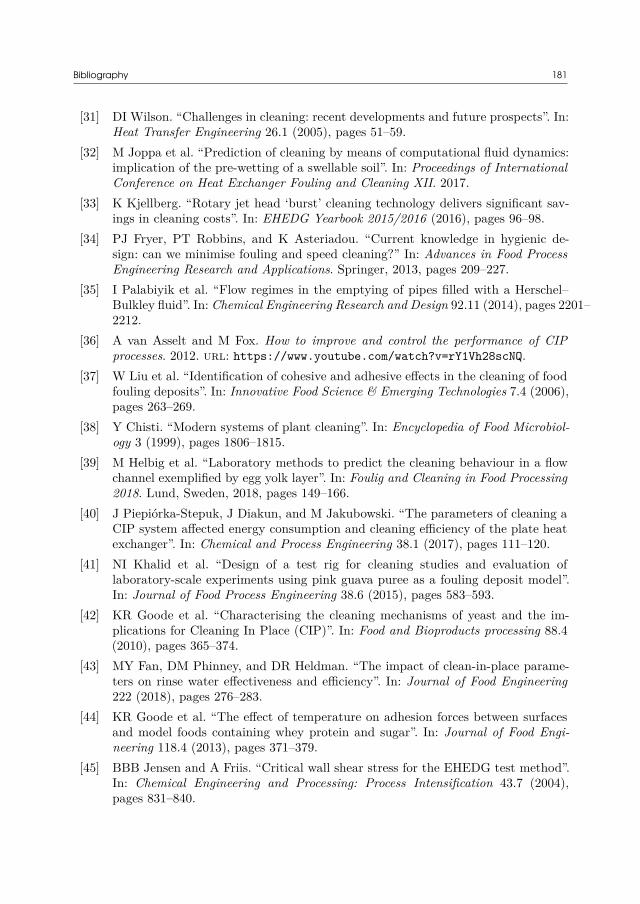
Bibliography 181
[31] DI Wilson. “Challenges in cleaning: recent developments and future prospects”. In:Heat Transfer Engineering 26.1 (2005), pages 51–59.
[32] M Joppa et al. “Prediction of cleaning by means of computational fluid dynamics:implication of the pre-wetting of a swellable soil”. In: Proceedings of InternationalConference on Heat Exchanger Fouling and Cleaning XII. 2017.
[33] K Kjellberg. “Rotary jet head ‘burst’ cleaning technology delivers significant sav-ings in cleaning costs”. In: EHEDG Yearbook 2015/2016 (2016), pages 96–98.
[34] PJ Fryer, PT Robbins, and K Asteriadou. “Current knowledge in hygienic de-sign: can we minimise fouling and speed cleaning?” In: Advances in Food ProcessEngineering Research and Applications. Springer, 2013, pages 209–227.
[35] I Palabiyik et al. “Flow regimes in the emptying of pipes filled with a Herschel–Bulkley fluid”. In: Chemical Engineering Research and Design 92.11 (2014), pages 2201–2212.
[36] A van Asselt and M Fox. How to improve and control the performance of CIPprocesses. 2012. url: https://www.youtube.com/watch?v=rY1Vh28scNQ.
[37] W Liu et al. “Identification of cohesive and adhesive effects in the cleaning of foodfouling deposits”. In: Innovative Food Science & Emerging Technologies 7.4 (2006),pages 263–269.
[38] Y Chisti. “Modern systems of plant cleaning”. In: Encyclopedia of Food Microbiol-ogy 3 (1999), pages 1806–1815.
[39] M Helbig et al. “Laboratory methods to predict the cleaning behaviour in a flowchannel exemplified by egg yolk layer”. In: Foulig and Cleaning in Food Processing2018. Lund, Sweden, 2018, pages 149–166.
[40] J Piepiórka-Stepuk, J Diakun, and M Jakubowski. “The parameters of cleaning aCIP system affected energy consumption and cleaning efficiency of the plate heatexchanger”. In: Chemical and Process Engineering 38.1 (2017), pages 111–120.
[41] NI Khalid et al. “Design of a test rig for cleaning studies and evaluation oflaboratory-scale experiments using pink guava puree as a fouling deposit model”.In: Journal of Food Process Engineering 38.6 (2015), pages 583–593.
[42] KR Goode et al. “Characterising the cleaning mechanisms of yeast and the im-plications for Cleaning In Place (CIP)”. In: Food and Bioproducts processing 88.4(2010), pages 365–374.
[43] MY Fan, DM Phinney, and DR Heldman. “The impact of clean-in-place parame-ters on rinse water effectiveness and efficiency”. In: Journal of Food Engineering222 (2018), pages 276–283.
[44] KR Goode et al. “The effect of temperature on adhesion forces between surfacesand model foods containing whey protein and sugar”. In: Journal of Food Engi-neering 118.4 (2013), pages 371–379.
[45] BBB Jensen and A Friis. “Critical wall shear stress for the EHEDG test method”.In: Chemical Engineering and Processing: Process Intensification 43.7 (2004),pages 831–840.
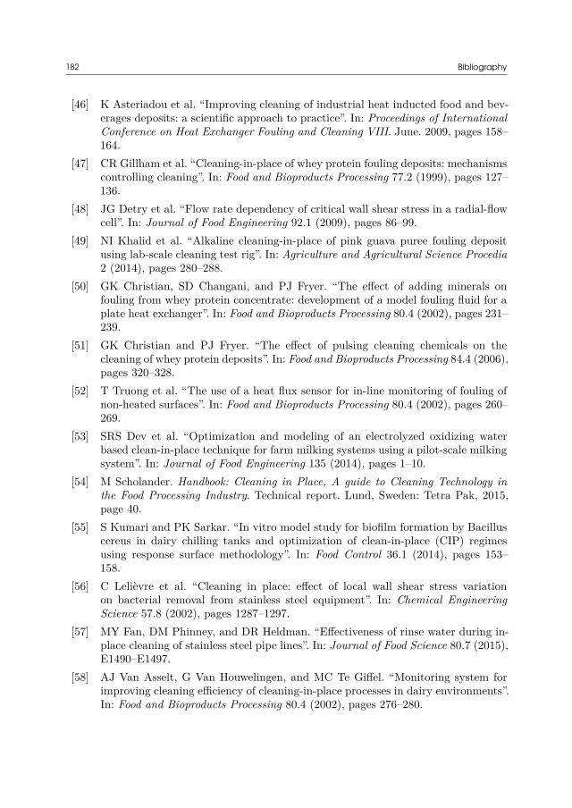
182 Bibliography
[46] K Asteriadou et al. “Improving cleaning of industrial heat inducted food and bev-erages deposits: a scientific approach to practice”. In: Proceedings of InternationalConference on Heat Exchanger Fouling and Cleaning VIII. June. 2009, pages 158–164.
[47] CR Gillham et al. “Cleaning-in-place of whey protein fouling deposits: mechanismscontrolling cleaning”. In: Food and Bioproducts Processing 77.2 (1999), pages 127–136.
[48] JG Detry et al. “Flow rate dependency of critical wall shear stress in a radial-flowcell”. In: Journal of Food Engineering 92.1 (2009), pages 86–99.
[49] NI Khalid et al. “Alkaline cleaning-in-place of pink guava puree fouling depositusing lab-scale cleaning test rig”. In: Agriculture and Agricultural Science Procedia2 (2014), pages 280–288.
[50] GK Christian, SD Changani, and PJ Fryer. “The effect of adding minerals onfouling from whey protein concentrate: development of a model fouling fluid for aplate heat exchanger”. In: Food and Bioproducts Processing 80.4 (2002), pages 231–239.
[51] GK Christian and PJ Fryer. “The effect of pulsing cleaning chemicals on thecleaning of whey protein deposits”. In: Food and Bioproducts Processing 84.4 (2006),pages 320–328.
[52] T Truong et al. “The use of a heat flux sensor for in-line monitoring of fouling ofnon-heated surfaces”. In: Food and Bioproducts Processing 80.4 (2002), pages 260–269.
[53] SRS Dev et al. “Optimization and modeling of an electrolyzed oxidizing waterbased clean-in-place technique for farm milking systems using a pilot-scale milkingsystem”. In: Journal of Food Engineering 135 (2014), pages 1–10.
[54] M Scholander. Handbook: Cleaning in Place, A guide to Cleaning Technology inthe Food Processing Industry. Technical report. Lund, Sweden: Tetra Pak, 2015,page 40.
[55] S Kumari and PK Sarkar. “In vitro model study for biofilm formation by Bacilluscereus in dairy chilling tanks and optimization of clean-in-place (CIP) regimesusing response surface methodology”. In: Food Control 36.1 (2014), pages 153–158.
[56] C Lelièvre et al. “Cleaning in place: effect of local wall shear stress variationon bacterial removal from stainless steel equipment”. In: Chemical EngineeringScience 57.8 (2002), pages 1287–1297.
[57] MY Fan, DM Phinney, and DR Heldman. “Effectiveness of rinse water during in-place cleaning of stainless steel pipe lines”. In: Journal of Food Science 80.7 (2015),E1490–E1497.
[58] AJ Van Asselt, G Van Houwelingen, and MC Te Giffel. “Monitoring system forimproving cleaning efficiency of cleaning-in-place processes in dairy environments”.In: Food and Bioproducts Processing 80.4 (2002), pages 276–280.
Bibliography 183
[59] KR Goode. “Characterising the cleaning behaviour of brewery foulants-to minimisethe cost of cleaning in place operations.” PhD thesis. University of Birmingham,2012.
[60] V Melero et al. “Experimental investigation about rinse water consumption ofa CIP process applied to a shell and tube exchanger”. In: Advanced MaterialsResearch. Volume 785. Trans Tech Publ. 2013, pages 1294–1298.
[61] L Suárez, MA Diez, and FA Riera. “Recovery of detergents in food industry: an in-dustrial approach”. In: Desalination and Water Treatment 56.4 (2015), pages 967–976.
[62] K Bader et al. “Online total organic carbon (TOC) as a process analytical tech-nology for cleaning validation risk management”. In: Pharmaceutical Engineering29.1 (2009), pages 8–20.
[63] E Wallhäußer et al. “Determination of cleaning end of dairy protein fouling usingan online system combining ultrasonic and classification methods”. In: Food andBioprocess Technology 7.2 (2014), pages 506–515.
[64] M Henningsson et al. “CFD simulation and ERT visualization of the displacementof yoghurt by water on industrial scale”. In: Journal of Food Engineering 80.1(2007), pages 166–175.
[65] Ecolab. 3D TRASAR Technology for CIP. Technical report. Ecolab USA Inc.,2017, page 3.
[66] A van Asselt. Cleaning Optimization OptCIP©: Reduce Cleaning Time and Pro-duction Costs. Technical report. Ede, Netherlands: NIZO food research B.V., 2014,page 2.
[67] Anderson,D. Conductivity Measurement: Critical for Clean-in-Place Systems. Tech-nical report. Irvine, Canada: Emerson Process Management, 2007, page 4.
[68] SP Lin and RD Reitz. “Drop and spray formation from a liquid jet”. In: AnnualReview of Fluid Mechanics 30.1 (1998), pages 85–105.
[69] RP Grant and S Middleman. “Newtonian jet stability”. In: AIChE Journal 12.4(1966), pages 669–678.
[70] A Chillman, M Ramulu, and M Hashish. “A general overview of waterjet surfacetreatment modeling”. In: American WJTA Conference and Expo. 2009.
[71] E Fuchs et al. “Influence of the nozzle distance on the cleaning result comparedto the jet break up and the mechanical forces on an industrial scale”. In: Foulingand Cleaning in Food Processing 2018. Lund, Sweden, 2018.
[72] DI Wilson et al. “Surface flow and drainage films created by horizontal impingingliquid jets”. In: Chemical Engineering Science 68.1 (2012), pages 449–460.
[73] RK Bhagat and DI Wilson. “Flow in the thin film created by a coherent turbulentwater jet impinging on a vertical wall”. In: Chemical Engineering Science 152(2016), pages 606–623.
[74] MWL Chee et al. “Impinging jet cleaning of tank walls: effect of jet length, wallcurvature and related phenomena”. In: Food and Bioproducts Processing (2018).
184 Bibliography
[75] DI Wilson et al. “Cleaning of soft-solid soil layers on vertical and horizontal sur-faces by stationary coherent impinging liquid jets”. In: Chemical Engineering Sci-ence 109 (2014), pages 183–196.
[76] DI Wilson et al. “Cleaning of a model food soil from horizontal plates by a movingvertical water jet”. In: Chemical Engineering Science 123 (2015), pages 450–459.
[77] HW Glover et al. “Cleaning of complex soil layers on vertical walls by fixedand moving impinging liquid jets”. In: Journal of Food Engineering 178 (2016),pages 95–109.
[78] NF Damkjær et al. “Flow pattern and cleaning performance of a stationary liquidjet operating at conditions relevant for industrial tank cleaning”. In: Food andBioproducts Processing 101 (2017), pages 145–156.
[79] SK Bhunia and JH Lienhard. “Splattering during turbulent liquid jet impingementon solid targets”. In: Journal of Fluids Engineering 116.2 (1994), pages 338–344.
[80] T Wang et al. “Flow patterns and draining films created by horizontal and inclinedcoherent water jets impinging on vertical walls”. In: Chemical Engineering Science102 (2013), pages 585–601.
[81] DE Hartley and W Murgatroyd. “Criteria for the break-up of thin liquid layersflowing isothermally over solid surfaces”. In: International Journal of Heat andMass Transfer 7.9 (1964), pages 1003–1015.
[82] KR Morison and RJ Thorpe. “Liquid distribution from cleaning-in-place spray-balls”. In: Food and Bioproducts Processing 80.4 (2002), pages 270–275.
[83] T Wang, JF Davidson, and DI Wilson. “Effect of surfactant on flow patterns anddraining films created by a static horizontal liquid jet impinging on a verticalsurface at low flow rates”. In: Chemical Engineering Science 88 (2013), pages 79–94.
[84] W Nusselt. “Die Oberflachenkondesation des Wasserdamffes”. In: Zeitschrift desVereines Deutscher Ingenieure 60 (1916), pages 541–546.
[85] S Portalski. “Studies of falling liquid film flow film thickness on a smooth verticalplate”. In: Chemical Engineering Science 18.12 (1963), pages 787–804.
[86] J Tihon et al. “Solitary waves on inclined films: their characteristics and the effectson wall shear stress”. In: Experiments in Fluids 41.1 (2006), pages 79–89.
[87] E Fuchs et al. “An experimental comparison of film flow parameters and cleaningbehaviour of falling liquid films for different tilt angles”. In: Food and BioproductsProcessing 93 (2015), pages 318–326.
[88] E Fuchs et al. “Influence of the film flow characteristic on the cleaning behaviour”.In: International Conference on Heat Exchanger Fouling and Cleaning X. 2013,pages 09–14.
[89] W Aouad et al. “Particle image velocimetry and modelling of horizontal coher-ent liquid jets impinging on and draining down a vertical wall”. In: ExperimentalThermal and Fluid Science 74 (2016), pages 429–443.
Bibliography 185
[90] J Tihon et al. “Electrodiffusion detection of the near-wall flow reversal in liquidfilms at the regime of solitary waves”. In: Journal of Applied Electrochemistry 33.7(2003), pages 577–587.
[91] JR Landel, H McEvoy, and SB Dalziel. “Cleaning of viscous drops on a flat inclinedsurface using gravity-driven film flows”. In: Food and Bioproducts Processing 93(2015), pages 310–317.
[92] AI Khuri and S Mukhopadhyay. “Response surface methodology”. In: Wiley Inter-disciplinary Reviews: Computational Statistics 2.2 (2010), pages 128–149.
[93] E Jurado Alameda et al. “Cleaning of starchy soils in clean-in-Place (CIP) systems:relationship between contact angle and detergency”. In: Journal of DispersionScience and Technology 37.3 (2016), pages 317–325.
[94] J Piepiórka-Stepuk, J Diakun, and S Mierzejewska. “Poly-optimization of cleaningconditions for pipe systems and plate heat exchangers contaminated with hot milkusing the Cleaning In Place method”. In: Journal of Cleaner Production 112 (2016),pages 946–952.
[95] E Martin, G Montague, and P Robbins. “A quality by design approach to pro-cess plant cleaning”. In: Chemical Engineering Research and Design 91.6 (2013),pages 1095–1105.
[96] D McCarthy. “Modern trends in CIP automation.” In: Food Quality and SafetyAugust (2015), pages 23–25.
[97] A Yang et al. “Towards improved cleaning of FMCG plants: a model-based ap-proach”. In: Computer Aided Chemical Engineering 25 (2008), page 1161.
[98] XM Wang et al. “Mathematical modeling and cycle time reduction of depositremoval from stainless steel pipeline during cleaning-in-place of milking systemwith electrolyzed oxidizing water”. In: Journal of Food Engineering 170 (2016),pages 144–159.
[99] C Lelièvre et al. “Cleaning-in-Place: modelling of cleaning kinetics of pipes soiledby Bacillus spores assuming a process combining removal and deposition”. In: Foodand Bioproducts Processing 80.4 (2002), pages 305–311.
[100] BBB Jensen et al. “Predicting cleaning: Estimate fluctuations in signal from elec-trochemical wall shear stress measurements using CFD”. In: Fouling, Cleaning &Disinfection in Food Processing. Department of Chemical Engineering, Universityof Cambridge. 2006, pages 130–137.
[101] BBB Jensen and A Friis. “Predicting the cleanability of mix-proof valves by use ofwall shear stress”. In: Journal of Food Process Engineering 28.2 (2005), pages 89–106.
[102] BBB Jensen, M Stenby, and DF Nielsen. “Improving the cleaning effect by chang-ing average velocity”. In: Trends in Food Science and Technology 18.Suppl. 1(2007).
[103] GZ Li et al. “Improving the efficiency of ‘clean-in-place’ procedures using a four-lobed swirl pipe: a numerical investigation”. In: Computers & Fluids 108 (2015),pages 116–128.
186 Bibliography
[104] GZ Li et al. “Optimization of a four-lobed swirl pipe for clean-in-place procedures”.In: ICCE 2015: International Conference on Clean Energy. 2015, page 561.
[105] GZ Li et al. “Large eddy simulation and Reynolds-averaged Navier–Stokes basedmodelling of geometrically induced swirl flows applied for the better understandingof Clean-In-Place procedures”. In: Food and Bioproducts Processing 104 (2017),pages 77–93.
[106] KR Davey, S Chandrakash, and BK O’Neill. “A new risk analysis of Clean-In-Placemilk processing”. In: Food Control 29.1 (2013), pages 248–253.
[107] H Xin. “A study of the mechanisms of chemical cleaning of milk protein foul-ing deposits using a model material (whey protein concentrate gel)”. PhD thesis.ResearchSpace@ Auckland, 2003.
[108] H Xin, XD Chen, and N Özkan. “Removal of a model protein foulant from metalsurfaces”. In: AIChE Journal 50.8 (2004), pages 1961–1973.
[109] KR Davey, S Chandrakash, and BK O’Neill. “A Friday 13th failure assessment ofclean-in-place removal of whey protein deposits from metal surfaces with auto-setcleaning times”. In: Chemical Engineering Science 126 (2015), pages 106–115.
[110] A Hill. Brewing microbiology: Managing microbes, ensuring quality and valorisingwaste. Woodhead Publishing, 2015.
[111] Great brewing process. url: https://carlsbergmyanmar.com.mm/en/beers-you-love/great-brewing-process/.
[112] Hatlar Group Pty Ltd. Clean-in-place best practice guidelines-Part I: Compare CIPwith best practice. Technical report August. Melbourne, Australia, 2010, page 40.
[113] JF Yang et al. “Anomaly analysis in cleaning-in-place operations of an industrialbrewery fermenter”. In: Industrial & Engineering Chemistry Research 57.38 (2018),pages 12871–12883.
[114] LH Chiang, EL Russell, and RD Braatz. Fault detection and diagnosis in industrialsystems. 2001.
[115] K Roy et al. “Multivariate statistical monitoring as applied to clean-in-place(CIP) and steam-in-place (SIP) operations in biopharmaceutical manufacturing”.In: Biotechnology Progress 30.2 (2014), pages 505–515.
[116] H Trevor, T Robert, and JH Friedman. The elements of statistical learning: datamining, inference, and prediction. 2009.
[117] C Undey and A Cinar. “Statistical monitoring of multistage, multiphase batchprocesses”. In: IEEE Control Systems 22.5 (2002), pages 40–52.
[118] J Ramsay. “Functional data analysis”. In: Encyclopedia of Statistics in BehavioralScience (2005).
[119] J Ramsay, G Hooker, and S Graves. Functional data analysis with R and MATLAB.Springer Science & Business Media, 2009.
[120] P Nomikos and JF MacGregor. “Multivariate SPC charts for monitoring batchprocesses”. In: Technometrics 37.1 (1995), pages 41–59.
Bibliography 187
[121] EJ Keogh and MJ Pazzani. “Derivative dynamic time warping”. In: Proceedings ofthe 2001 SIAM International Conference on Data Mining. SIAM. 2001, pages 1–11.
[122] SW Wang and F Xiao. “AHU sensor fault diagnosis using principal componentanalysis method”. In: Energy and Buildings 36.2 (2004), pages 147–160.
[123] C Ündey, S Ertunç, and A Çınar. “Online batch/fed-batch process performancemonitoring, quality prediction, and variable-contribution analysis for diagnosis”.In: Industrial & Engineering Chemistry Research 42.20 (2003), pages 4645–4658.
[124] S Wold et al. “Modelling and diagnostics of batch processes and analogous kineticexperiments”. In: Chemometrics and Intelligent Laboratory Systems 44.1-2 (1998),pages 331–340.
[125] SP Gurden et al. “A comparison of multiway regression and scaling methods”. In:Chemometrics and Intelligent Laboratory Systems 59.1-2 (2001), pages 121–136.
[126] Ch Zhao and FR Gao. “Fault-relevant principal component analysis (FPCA) methodfor multivariate statistical modeling and process monitoring”. In: Chemometricsand Intelligent Laboratory Systems 133 (2014), pages 1–16.
[127] P Miller, RE Swanson, and CE Heckler. “Contribution plots: a missing link inmultivariate quality control”. In: Applied Mathematics and Computer Science 8.4(1998), pages 775–792.
[128] ME Celebi and K Aydin. Unsupervised learning algorithms. Springer, 2016.[129] RP Singh and DR Heldman. Introduction to Food Engineering. 5th edition. Aca-
demic Press, 2014, page 892.[130] A Lehman et al. JMP for basic univariate and multivariate statistics: Methods for
researchers and social scientists. SAS Institute, 2013.[131] JA Westerhuis, SP Gurden, and AK Smilde. “Generalized contribution plots in
multivariate statistical process monitoring”. In: Chemometrics and Intelligent Lab-oratory Systems 51.1 (2000), pages 95–114.
[132] P Van den Kerkhof et al. “Analysis of smearing-out in contribution plot basedfault isolation for statistical process control”. In: Chemical Engineering Science104 (2013), pages 285–293.
[133] A Kassidas, JF MacGregor, and PA Taylor. “Synchronization of batch trajectoriesusing dynamic time warping”. In: AIChE Journal 44.4 (1998), page 864.
[134] JF Yang et al. “CFD modelling of axial mixing in the intermediate and final rinsesof cleaning-in-place procedures of straight pipes”. In: Journal of Food Engineering221 (2018), pages 95–105.
[135] JF Yang et al. “Investigation of the cleaning of egg yolk deposits from tank surfacesusing continuous and pulsed flows”. In: Food and Bioproducts Processing (2018).
[136] L Chen et al. “Cleaning in place with onsite-generated electrolysed oxidizing waterfor water-saving disinfection in breweries”. In: Journal of the Institute of Brewing118.4 (2012), pages 401–405.
188 Bibliography
[137] J Wiklund, M Stading, and C Trägårdh. “Monitoring liquid displacement of modeland industrial fluids in pipes by in-line ultrasonic rheometry”. In: Journal of FoodEngineering 99.3 (2010), pages 330–337.
[138] TO Salmi, JP Mikkola, and JP Warna. Chemical reaction engineering and reactortechnology. CRC Press, 2010.
[139] GI Taylor. “Dispersion of soluble matter in solvent flowing slowly through a tube”.In: Proceedings of the Royal Society A 219.1137 (1953), pages 186–203.
[140] O Levenspiel. “Longitudinal mixing of fluids flowing in circular pipes”. In: Indus-trial & Engineering Chemistry 50.3 (1958), pages 343–346.
[141] LL Zhao, J Derksen, and R Gupta. “Simulations of axial mixing of liquids in along horizontal pipe for industrial applications”. In: Energy & Fuels 24.11 (2010),pages 5844–5850.
[142] Y Chisti and M Moo-Young. “Clean-in-place systems for industrial bioreactors: de-sign, validation and operation”. In: Journal of Industrial Microbiology 13.4 (1994),pages 201–207.
[143] DC Wilcox. Turbulence Modeling for CFD. DCW Industries, 20016.[144] BBB Jensen. “Numerical study of influence of inlet turbulence parameters on
turbulence intensity in the flow domain: incompressible flow in pipe system”. In:Proceedings of the Institution of Mechanical Engineers, Part E: Journal of ProcessMechanical Engineering 221.4 (2007), pages 177–186.
[145] Z Stegowski et al. “Dispersion determination in a turbulent pipe flow using ra-diotracer data and CFD analysis”. In: Computers & Fluids 79 (2013), pages 77–81.
[146] B James and F Ollis David. Biochemical Engineering Fundamentals. Mc Grow HillBook Company, 1986.
[147] A Graßhoff. “Toträume in CIP-gereinigten Rohrleitungssystemen”. In: DeutscheMilchwirtschaft 13 (1983), pages 407–414.
[148] R Higbie. “The rate of absorption of a pure gas into a still liquid during shortperiods of exposure”. In: Transactions of AIChE 31 (1935), pages 365–389.
[149] EP Van Elk, MC Knaap, and GF Versteeg. “Application of the penetration theoryfor gas–liquid mass transfer without liquid bulk: differences with systems with abulk”. In: Chemical Engineering Research and Design 85.4 (2007), pages 516–524.
[150] K Ekambara and JB Joshi. “Axial mixing in laminar pipe flows”. In: ChemicalEngineering Science 59.18 (2004), pages 3929–3944.
[151] M Assar et al. “A new approach to analyze entrance region mass transfer withina falling film”. In: Heat and Mass Transfer 50.5 (2014), pages 651–660.
[152] BBB Jensen et al. “Local wall shear stress variations predicted by computationalfluid dynamics for hygienic design”. In: Food and Bioproducts Processing 83.1(2005), pages 53–60.
[153] M Schöler et al. “Local analysis of cleaning mechanisms in CIP processes”. In: Foodand Bioproducts Processing 90.4 (2012), pages 858–866.

Bibliography 189
[154] R Darby and RP Chhabra. Chemical Engineering Fluid Mechanics. Edited by RDarby and RP Chhabra. 3rd edition. CRC Press, 2017, page 555.
[155] DC Rennels and HM Hudson. Pipe Flow: A Practical and Comprehensive Guide.John Wiley & Sons, 2012.
[156] Neutrium. Pressure loss from fittings - expansion and reduction in pipe size.url: https://neutrium.net/fluid_flow/pressure-loss-from-fittings-expansion-and-reduction-in-pipe-size/.
[157] DF Young et al. A Brief Introduction to Fluid Mechanics. John Wiley & Sons,2010.
[158] Crane Company. Flow of fluids through valves, fittings, and pipe. 410. Crane Com-pany, 1978.
[159] A Graßhoff. “Untersuchungen zum Stromungsverhalten von Flussigkeiten in zylin-drischen Totraumen von Rorhleitungssystemen”. In: Die Kieler MilchwirtschaftForschungs 32.4 (1980), pages 273–298.
[160] DE Briggs et al. Brewing: science and practice. Elsevier, 2004.[161] M Stenby, MW Dethlefsen, BBB Jensen, et al. “New test method for rotating spray
head performance in tank cleaning”. In: World Congress on Hygienic Engineering& Design. 2011, pages 40–43.
[162] CR Gillham et al. “Enhanced cleaning of whey protein soils using pulsed flows”.In: Journal of Food Engineering 46.3 (2000), pages 199–209.
[163] K Bode et al. “Pulsed flow cleaning of whey protein fouling layers”. In: Proceed-ings of 6th International Conference on Heat Exchanger Fouling and Cleaning -Challenges and Opportunities. Volume 2. 25. Kloster Irsee, Germany, The BerkeleyElectronic Press, 2005, pages 165–173.
[164] W Augustin et al. “Pulsed flow for enhanced cleaning in food processing”. In: Foodand Bioproducts Processing 88.4 (2010), pages 384–391.
[165] H Föste et al. “Modeling and validation of the mechanism of pulsed flow cleaning”.In: Heat Transfer Engineering 34.8-9 (2013), pages 753–760.
[166] MS Celnik et al. “Analytical approaches for calculation of shear stress enhancementin laminar pulsed flows”. In: Proceedings of 6th International Conference on HeatExchanger Fouling and Cleaning - Challenges and Opportunities. Kloster Irsee,2005, pages 174–182.
[167] B Olayiwola and P Walzel. “Effects of in-phase oscillation of retentate and filtratein crossflow filtration at low Reynolds number”. In: Journal of Membrane Science345.1-2 (2009), pages 36–46.
[168] C Weidemann, S Vogt, and H Nirschl. “Cleaning of filter media by pulsed flow–Establishment of dimensionless operation numbers describing the cleaning result”.In: Journal of Food Engineering 132 (2014), pages 29–38.
[169] E Fuchs et al. “Erhöhung der Reinigungseffizienz bei der Cleaning-in-Place-Reinigungdurch diskontinuierliche Flüssigkeitsstrahlen”. In: Chemie Ingenieur Technik 89.8(2017), pages 1072–1082.
190 Bibliography
[170] H Stoye et al. “Untersuchungen zur Steigerung der Reinigungseffizienz durchpulsierende Spritzreinigung”. In: Chemie Ingenieur Technik 86.5 (2014), pages 707–713.
[171] M Le Denmat, M Anton, and G Gandemer. “Protein denaturation and emulsifyingproperties of plasma and granules of egg yolk as related to heat treatment”. In:Journal of Food Science 64.2 (1999), pages 194–197.
[172] DC Montgomery. Design and Analysis of Experiments. 8th edition. John Wiley &Sons, Inc., 2012, page 757.
[173] K Lerch et al. “Cleanability of surfaces from active pharmaceutical ingredientsurrogate riboflavin by falling film”. In: Chemie Ingenieur Technik 85.3 (2013),pages 323–332.
[174] Diversey CIPTEC. url: https://www.diversey.com/food- care/diversey-knowledge-based-services/diversey-ciptec.
[175] L Pettigrew et al. “Optimisation of water usage in a brewery clean-in-place systemusing reference nets”. In: Journal of Cleaner Production 87 (2015), pages 583–593.
[176] JT Holah et al. “A method for assessing the in-place cleanability of food-processingequipment”. In: Trends in Food Science & Technology 18 (January 2007), S54–S58.
[177] T Varzakas and C Tzia. Handbook of food processing: food safety, quality, andmanufacturing processes. CRC Press, 2015.
[178] RK Bhagat, AM Perera, and DI Wilson. “Cleaning vessel walls by moving wa-ter jets: Simple models and supporting experiments”. In: Food and BioproductsProcessing 102 (2017), pages 31–54.
[179] H Köhler et al. “Study on the application of cleaning models with high speed waterjets to CIP-processes”. In: Tehnički Vjesnik 23.2 (2016), pages 349–355.
[180] T Wang, JF Davidson, and DI Wilson. “Flow patterns and cleaning behaviourof horizontal liquid jets impinging on angled walls”. In: Food and BioproductsProcessing 93 (2015), pages 333–342.
[181] OM Magens et al. “Adhesion and cleaning of foods with complex structure: Effectof oil content and fluoropolymer coating characteristics on the detachment of cakefrom baking surfaces”. In: Journal of Food Engineering 197 (2017), pages 48–59.
[182] Micro-Epsilon. “Instruction Manual: confocalDT 2451/2461/2471”. Ortenburg, Ger-many, 2016.
[183] TT Hsu et al. “Role of fluid elasticity on the dynamics of rinsing flow by animpinging jet”. In: Physics of Fluids 23.3 (2011), page 033101.
[184] The American Society of Mechanical Engineers. ASME BPE-2016: BioprocessingEquipment. Standard. 2016.
[185] G Götz et al. “Adjustment of the wastewater matrix for optimization of membranesystems applied for water reuse in breweries”. In: Journal of Membrane Science465 (2014), pages 68–77.
Bibliography 191
[186] K Loganathan, P Chelme-Ayala, and MG El-Din. “Pilot-scale study on the treat-ment of basal aquifer water using ultrafiltration, reverse osmosis and evapora-tion/crystallization to achieve zero-liquid discharge”. In: Journal of EnvironmentalManagement 165 (2016), pages 213–223.
[187] L Suárez et al. “Membrane technology for the recovery of detergent compounds: areview”. In: Journal of Industrial and Engineering Chemistry 18.6 (2012), pages 1859–1873.
[188] M Dresch, G Daufin, and B Chaufer. “Integrated membrane regeneration processfor dairy cleaning-in-place”. In: Separation and Purification Technology 22 (2001),pages 181–191.
[189] T Paul et al. “Smart cleaning-in-place process through crude keratinase: an eco-friendly cleaning techniques towards dairy industries”. In: Journal of Cleaner Pro-duction 76 (2014), pages 140–153.
[190] T Chutrakul et al. “Enzyme-based integrated solution to cleaning of coconut milkfoulants”. In: Food and Bioproducts Processing (2018).
[191] R Jiménez-Pichardo et al. “Evaluation of electrolyzed water as cleaning and disin-fection agent on stainless steel as a model surface in the dairy industry”. In: FoodControl 60 (2016), pages 320–328.
[192] J Quarini. “Ice-pigging to reduce and remove fouling and to achieve clean-in-place”.In: Applied Thermal Engineering 22.7 (2002), pages 747–753.
[193] EA Ainslie et al. “Heat exchanger cleaning using ice pigging”. In: Proceedings ofInternational Conference on Heat Exchanger Fouling and Cleaning VIII. 2009,pages 433–438.


Process and Systems Engineering Centre (PROSYS)Department of Chemical and Biochemical EngineeringTechnical University of DenmarkSøltofts Plads, Building 229DK - 2800 Kgs. LyngbyDenmark Phone: +45 45 25 28 00Web: www.kt.dtu.dk/forskning/prosys