model to estimate carbon in organic soils sequestration ... user man… · model to estimate carbon...

1

Model to Estimate Carbon in Organic

Soils – Sequestration and Emissions

(ECOSSE).

User-Manual August 2010 Issue

Smith J, Gottschalk P, Bellarby J, Richards M, Nayak D, Coleman K, Hillier J, Flynn H, Wattenbach M,

Aitkenhead M, Yeluripurti J, Farmer J, Smith P

Contact: Jo Smith

Address: Institute of Biological and Environmental Sciences,

School of Biological Sciences,

University of Aberdeen,

23 St Machar Drive, Room G45

Aberdeen,

AB24 3UU,

Scotland,

UK

Tel: +44 (0)1224 272702

Fax: +44 (0)1224 272703

E-mail: [email protected]

2

WWW: http://www.abdn.ac.uk/ibes/staff/jo.smith/ECOSSE

Contents

PART A - MODEL DESCRIPTION ............................................................................................................. 11

A1 Introduction ..................................................................................................................................... 11

A1.1 Importance of long term estimates of aerobic decomposition ................................................ 11

A1.2 The ECOSSE approach ............................................................................................................... 11

A2 The activity of soil organic matter decomposition .......................................................................... 13

A2.1 Definition of pools used in ECOSSE ........................................................................................... 13

A2.2 Determining the initial sizes of soil organic matter pools ........................................................ 14

A2.2.1 Rapid determination of initial soil organic matter pool sizes ............................................ 14

A2.2.2 Initialization by full ECOSSE simulation .............................................................................. 16

A2.3 Evaluation of the methods used to determine the initial sizes of the soil organic matter pools

........................................................................................................................................................... 17

A3 Aerobic decomposition of soil organic matter pools ....................................................................... 18

A3.1 Impact of soil water on aerobic decomposition ....................................................................... 19

A3.2 Impact of soil temperature on aerobic decomposition ............................................................ 21

A3.3 Impact of soil pH on aerobic decomposition ............................................................................ 21

A3.4 Impact of crop cover on aerobic decomposition ...................................................................... 23

A3.5 Impact of nitrogen on aerobic decomposition ......................................................................... 24

A3.6 Impact of clay content on aerobic decomposition ................................................................... 25

A3.7 Evaluation of ECOSSE simulations of aerobic decomposition .................................................. 26

A4 Anaerobic decomposition of soil organic matter pools ................................................................... 26

A4.1 Impact of soil water on anaerobic decomposition ................................................................... 27

A4.2 Impact of soil temperature on anaerobic decomposition ........................................................ 28

A4.3 Impact of soil pH on anaerobic decomposition ........................................................................ 30

A4.4 Impact of crop cover on anaerobic decomposition .................................................................. 31

A4.5 Impact of nitrogen on anaerobic decomposition ..................................................................... 31

A4.6 Impact of clay content on anaerobic decomposition ............................................................... 31

A4.7 Impact of oxygen on methane emissions ................................................................................. 31

A4.8 Evaluation of ECOSSE simulations of anaerobic decomposition .............................................. 32

A5 Nitrogen transformations ................................................................................................................ 32

A5.1 Mineralisation / Immobilisation ................................................................................................ 32

3

A5.2 Nitrification ............................................................................................................................... 32

A5.3 Denitrification ........................................................................................................................... 35

A5.4 Nitrate leaching ......................................................................................................................... 38

A5.5 Leaching of dissolved organic matter ....................................................................................... 38

A5.6 Ammonia volatilisation ............................................................................................................. 41

A5.6.1 Volatilisation loss from applied manure ............................................................................ 41

A5.6.2 Volatilisation loss from fertiliser ........................................................................................ 42

A5.7 Crop nitrogen uptake ................................................................................................................ 43

A5.7.1 Plant Inputs ........................................................................................................................ 43

A5.7.2 Timing of Management Events .......................................................................................... 43

A.5.7.3 Fertiliser Applications ........................................................................................................ 43

A.5.7.4 Pattern of Debris Incorporation ........................................................................................ 44

A.5.7.5 Pattern of Nitrogen Uptake .............................................................................................. 46

A5.8 Senescence ................................................................................................................................ 46

A5.9 Evaluation of ECOSSE simulations of nitrogen transformations ............................................... 46

A6 Water Movement ............................................................................................................................. 47

A6.1 Vertical water movement ......................................................................................................... 47

A6.2 Restricted flow .......................................................................................................................... 47

A6.3 Evaluation of ECOSSE simulations of water movement ........................................................... 48

PART B - SITE SPECIFIC SIMULATIONS ................................................................................................... 48

B1 Input files .......................................................................................................................................... 48

B1.1 Management Data .................................................................................................................... 48

B1.1.1 Input through file MANAGEMENT.DAT .............................................................................. 48

B1.1.2 Input by setup file .............................................................................................................. 49

B1.2. Weather Data ........................................................................................................................... 50

B1.3 Crop Parameters ....................................................................................................................... 50

B1.4 Soil Parameters ......................................................................................................................... 52

B2 Output files ....................................................................................................................................... 52

PART C - LIMITED DATA SITE SIMULATIONS .......................................................................................... 54

C1 Input files .......................................................................................................................................... 54

C1.1 Site and management data ....................................................................................................... 54

C1.2 Weather data ............................................................................................................................ 58

C2 Output files ....................................................................................................................................... 58

PART D - SPATIAL SIMULATIONS ........................................................................................................... 59

4

D1 Input files ......................................................................................................................................... 59

D1.1 File GNAMES.DAT ...................................................................................................................... 59

D1.2 Input File for NPP and Soil Information .................................................................................... 59

D1.3 Format of Input File for LU Information ................................................................................... 60

D1.4 Format of Input File for Soil Codes ........................................................................................... 61

D1.4.1 Non SSKIB Data .................................................................................................................. 61

D1.4.2 SSKIB Data .......................................................................................................................... 62

D1.5 Format of Input File for Future Climate .................................................................................... 63

D1.5.1 Scottish non-SSKIB and SSKIB ............................................................................................ 63

D1.5.2 Format of Input File for Future Rainfall (JULES run) .......................................................... 64

D1.5.3 Format of Input File for Future Temperature (JULES run) ................................................. 64

D1.5.4 Format of Input File for Net Primary Production (JULES run) ............................................ 64

D2 Output files ...................................................................................................................................... 64

D2.1 Format of Output File for Results on 1km2 grid ........................................................................ 64

D2.2 Format of Output File for Results on 20km2 grid ...................................................................... 67

D2.3 Format of Output File for C Change data (“CHANGE.OUT”) ..................................................... 68

D2.4 Format of Climate Change Results file ...................................................................................... 69

D2.5 Format of File for Calculation of Effects of Different Mitigation Options (files named

MIT_A2P.OUT etc) ............................................................................................................................. 69

PART E - REFERENCES ............................................................................................................................ 70

5

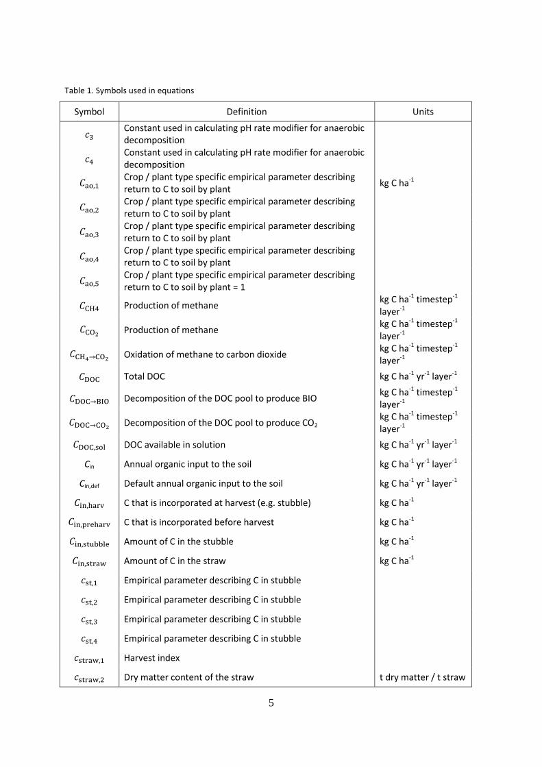
Table 1. Symbols used in equations

Symbol Definition Units

Constant used in calculating pH rate modifier for anaerobic decomposition

Constant used in calculating pH rate modifier for anaerobic decomposition

Crop / plant type specific empirical parameter describing return to C to soil by plant

kg C ha-1




Crop / plant type specific empirical parameter describing return to C to soil by plant = 1

Production of methane kg C ha-1 timestep-1 layer-1

Production of methane kg C ha-1 timestep-1 layer-1

Oxidation of methane to carbon dioxide kg C ha-1 timestep-1 layer-1

Total DOC kg C ha-1 yr-1 layer-1

Decomposition of the DOC pool to produce BIO kg C ha-1 timestep-1 layer-1

Decomposition of the DOC pool to produce CO2 kg C ha-1 timestep-1 layer-1

DOC available in solution kg C ha-1 yr-1 layer-1

Cin Annual organic input to the soil kg C ha-1 yr-1 layer-1

Cin,def Default annual organic input to the soil kg C ha-1 yr-1 layer-1

C that is incorporated at harvest (e.g. stubble) kg C ha-1

C that is incorporated before harvest kg C ha-1

Amount of C in the stubble kg C ha-1

Amount of C in the straw kg C ha-1

Empirical parameter describing C in stubble




Harvest index

Dry matter content of the straw t dry matter / t straw

6


C : dry matter ratio of the straw kg C / t straw dry matter

N : dry matter ratio of the straw kg N / t straw dry matter

Total annual organic inputs to the soil kg C ha-1 yr-1

C in the IOM pool kg C ha-1 layer-1

C in decomposing SOM pool, R kg C ha-1 layer-1

Concentration of C in decomposing SOM pool, R kg C ha-1 layer-1

Concentration of C in decomposing SOM pool, R, at start of the time step

kg C ha-1 layer-1

Concentration of C in decomposing SOM pool, R, at end of time step t

kg C ha-1 layer-1

Typical C:N ratio of bacteria

Typical C:N ratio of fungi

C:N ratios for the different land uses

Stable C:N ratio of the SOM

Ctot,meas Measured total soil carbon kg C ha-1 layer-1

Ctot,sim Simulated total soil carbon kg C ha-1 layer-1

Soil dependent factor that accounts for different rates of CH4 diffusion and oxidation

Depth of CH4 production cm

Depth at which soil becomes a net methane sink cm

Excess drainage when water flow is unrestricted compared to when water flow is restricted

mm layer-1

Unrestricted drainage from layer i mm layer-1

Water drained with restriction to drainage mm layer-1

Water drained with no restriction to drainage mm layer-1

Decomposition efficiency

Fraction representing the efficiency of decomposition of DOC to BIO

Rate constant for aerobic decomposition of BIO pool time step-1

Rate constant for anaerobic decomposition of BIO pool time step-1

Rate constant for decomposition of DOC into BIO time step-1

Rate constant for the incorporation of C in debris before harvest

Rate constant for aerobic decomposition of DPM pool time step-1

Rate constant for anaerobic decomposition of DPM pool time step-1

7


Rate constant for aerobic decomposition of HUM pool time step-1

Rate constant for the incorporation of N in debris before harvest

Rate constant for anaerobic decomposition of HUM pool time step-1

Rate constant for aerobic decomposition of SOM pool time step-1

Rate constant for anaerobic decomposition of SOM pool time step-1

Rate constant for DOC production from SOM pool time step-1

Rate constant for aerobic decomposition of RPM pool time step-1

Rate constant for anaerobic decomposition of RPM pool time step-1

Denitrification rate modifier due to biological activity

Aerobic decomposition rate modifier due to crop cover

Anaerobic decomposition rate modifier due to crop cover

Rate modifier due to crop cover for production of DOC

Nitrification rate modifier due to ammonium

Denitrification rate modifier due to nitrate

Aerobic decomposition rate modifier due to soil pH

Anaerobic decomposition rate modifier due to soil pH

Nitrification rate modifier due to soil pH

Rate modifier due to soil pH for production of DOC

Minimum value for aerobic decomposition rate modifier according to pH

Aerobic decomposition rate modifier due to soil temperature

Anaerobic decomposition rate modifier due to soil temperature

Nitrification rate modifier due to soil temperature

Rate modifier due to soil temperature for production of DOC

Aerobic decomposition rate modifier due to soil moisture

Anaerobic decomposition rate modifier due to soil moisture

Nitrification rate modifier due to soil moisture

Denitrification rate modifier due to soil moisture

Rate modifier due to soil moisture for production of DOC

Aerobic decomposition rate modifier due to soil moisture at permanent wilting point

Nitrification rate modifier due to soil moisture at

8


permanent wilting point

Soil factor accounting for diffusion and oxidation of methane

cm-1

The number of the deepest layer in the soil profile

Amount of nitrogen emitted from the soil during denitrification

kg N ha-1 layer-1 timestep-1

Amount of N2 gas lost by denitrification kg N ha-1 layer-1 timestep-1

Amount of N2O gas lost by denitrification kg N ha-1 layer-1 timestep-1

Proportion of N2O produced due to partial nitrification at field capacity

Amount of fertiliser N applied kg N ha-1 timestep-1

Proportion of full nitrification lost as gas

N that is incorporated at harvest (e.g. stubble) kg N ha-1

N that is incorporated before harvest kg N ha-1

Total annual organic inputs to the soil kg N ha-1 yr-1

Nitrogen in straw kg N ha-1

The amount of N nitrified in the layer kg N ha-1 layer-1 timestep-1

The amount of nitrified N emitted as N2O in the layer kg N ha-1 layer-1 timestep-1

The amount of nitrified N emitted as NO in the layer kg N ha-1 layer-1 timestep-1

Concentration of ammonium in the soil kg N ha-1 layer-1

Proportion of full nitrification gaseous loss lost as NO

Concentration of nitrate in the soil kg N ha-1 layer-1

Total plant N requirement in above ground parts of the plant

kg N ha-1 year-1

Total plant N requirement in below ground parts of the plant

kg N ha-1 year-1

Total plant N requirement kg N ha-1 year-1

Ammonium lost by volatilisation from added manure kg N ha-1 timestep-1

Proportion of ammonium sulphate in the fertiliser

Proportion of bacteria in the soil

Minimum proportion of bacteria found in the soil

Maximum proportion of bacteria found in the soil

Proportion of BIO produced on aerobic decomposition kg C (kg C decomp.)-1

9


Proportion of clay in the soil kg clay (kg soil)-1

Proportion of CO2 produced on aerobic decomposition kg C (kg C decomp.)-1

Proportion of fungi in the soil

Soil pH

Critical threshold pH below which rate of DOC production starts to decrease

Critical threshold pH below which rate of aerobic decomposition starts to decrease

pH at which rate of aerobic decomposition is at minimum rate

pH at which rate of DOC production is at minimum rate

Optimum soil pH for decomposition

Sensitivity of the decomposition processes in this soil to pH

Proportion of HUM produced on aerobic decomposition kg C (kg C decomp.)-1

Proportion of N in above ground crop that is incorporated in the soil

Proportion of N in below ground crop that is incorporated in the soil

Proportion of nitrate N to total denitrification at which N2 emissions fall to zero

Proportion of denitrified N lost as N2 at field capacity

Proportion of ammonium in the manure

Proportions of denitrified gas emitted as N2 according to the nitrate content of the soil

Proportion restriction in drainage at a particular site

Proportion of urea in the fertiliser

Proportion of denitrified gas emitted as N2 according to the water content of the soil

Amount of water held in a particular soil layer above the permanent wilting point

mm layer-1

Amount of water held in a layer between field capacity and the soil at -100 kPa

mm layer-1

Amount of water held in a layer between field capacity and the permanent wilting point

mm layer-1

Amount of water held in a layer between saturation and the permanent wilting point

mm layer-1

is a constant, describing the response of a process to temperature

Volatilisation quotient for manure

Volatilisation quotient for urea fertiliser

Volatilisation quotient for ammonium sulphate fertiliser

10


Amount of rainfall mm timestep-1

Critical level of rainfall below which volatilisation starts. mm timestep-1

Size of the time step seconds

Mean air temperature for the period in the timestep C

Mean soil temperature for the period in the timestep C

Cumulative air temperature C days

Methane transport factor

Empirical parameter describing the sigmoid uptake of N by the crop

Empirical parameter describing the sigmoid uptake of N by the crop

Empirical parameter describing uptake of N in below ground parts of the plant



Empirical parameter describing uptake of N in above ground parts of the plant



Weeks till harvest

Fresh weight of manure added t ha-1

Crop Yield t ha-1

11

PART A - MODEL DESCRIPTION

A1 Introduction

A1.1 Importance of long term estimates of aerobic decomposition Climate change, caused by greenhouse gas (GHG) emissions, is one of the most serious threats facing

our planet, and is of concern at both UK and devolved administration levels. Accurate predictions for

the effects of changes in climate and land use on GHG emissions are vital for informing land use

policy. Models that are currently used to predict differences in soil carbon (C) and nitrogen (N)

caused by these changes, have been derived from those based on mineral soils or ‘true’ deep peat. It

has been suggested that none of these models is entirely satisfactory for describing what happens to

organic soils following land-use change.

Globally peatland covers approximately 4 million km², with a total C stock of ~450 Pg C in 2008

(Joosten, 2009). Peat is found across the planet with Russia, Canada, Indonesia and the United States

having the largest peatland areas totalling just under 3 million km² (Joosten, 2009). Northern

peatlands are the most important terrestrial C store. It is estimated that 20-30% of the global

terrestrial C is held in 3% of its land area (Gorham, 1991). Over the Holocene, northern peatlands

have accumulated C at a rate of 960 Mt C yr-1 on average, making this ecosystem not only a

substantial store of C, but also a large potential sink for atmospheric C (Gorham, 1991). Reports of

Scottish GHG emissions have revealed that approximately 15% of Scotland’s total emissions come

from land use changes on Scotland’s high C soils (Smith et al, 2007). It is therefore important to

reduce the major uncertainty in assessing the C store and flux from land use change on organic soils,

especially those which are too shallow to be true peats but still contain a potentially large reserve of

C.

In order to predict the response of organic as well as mineral soils to external change we need

models that more accurately reflect the conditions of these soils. Here we present a model for both

organic and mineral soils that will help to provide more accurate values of net change to soil C and N

in response to changes in land use and climate and may be used to inform reporting to GHG

inventories. The main aim of the model described here is to simulate the impacts of land-use and

climate change on GHG emissions from these types of soils, as well as mineral and peat soils. The

model is a) driven by commonly available meteorological data and soil descriptions, b) able to predict

the impacts of land-use change and climate change on C and N stores in organic and mineral soils,

and c) able to function at national scale as well as field scale, so allowing results to be used to directly

inform policy decisions.

A1.2 The ECOSSE approach

The ECOSSE model was developed to simulate highly organic soils from concepts originally derived

for mineral soils in the RothC (Jenkinson and Rayner, 1977; Jenkinson et al. 1987; Coleman and

Jenkinson, 1996) and SUNDIAL (Bradbury et al. 1993; Smith et al. 1996) models. Following these

established models, ECOSSE uses a pool type approach, describing soil organic matter (SOM) as pools

of inert organic matter, humus, biomass, resistant plant material and decomposable plant material

Fig 1a).

12

Fig 1b. Structure of the nitrogen components of ECOSSE

Figure 1a. Structure of the carbon components of ECOSSE

13

All of the major processes of C and N turnover in the soil are included in the model, but each of the

processes is simulated using only simple equations driven by readily available input variables,

allowing it to be developed from a field based model to a national scale tool, without high loss of

accuracy. ECOSSE differs from RothC and SUNDIAL in the addition of descriptions of a number of

processes and impacts that are not important in the mineral arable soils that these models were

originally developed for. More importantly, ECOSSE differs from RothC and SUNDIAL in the way that

it makes full use of the limited information that is available to run models at national scale. In

particular, measurements of soil C are used to interpolate the activity of the SOM and the plant

inputs needed to achieve those measurements. Any data available describing soil water, plant inputs,

nutrient applications and timing of management operations are used to drive the model and so

better apportion the factors determining the interpolated activity of the SOM. However, if any of this

information is missing, the model can still provide accurate simulations of SOM turnover, although

the impact of changes in conditions will be estimated with less accuracy due to the reduced detail of

the inputs. This novel approach will be discussed further below.

In summary, during the decomposition process, material is exchanged between the SOM pools

according to first order rate equations, characterised by a specific rate constant for each pool, and

modified according to rate modifiers dependent on the temperature, moisture, crop cover and pH of

the soil. Under aerobic conditions, the decomposition process results in gaseous losses of carbon

dioxide (CO2); under anaerobic conditions losses as methane (CH4) dominate. The N content of the

soil follows the decomposition of the SOM (Fig 1b), with a stable C:N ratio defined for each pool at a

given pH, and N being either mineralised or immobilised to maintain that ratio. Nitrogen released

from decomposing SOM as ammonium (NH4+) or added to the soil may be nitrified to nitrate (NO3

-).

Carbon and N may be lost from the soil by the processes of leaching (NO3-, dissolved organic C (DOC),

and dissolved organic N (DON)), denitrification, volatilisation or crop offtake, or C and N may be

returned to the soil by plant inputs, inorganic fertilizers, atmospheric deposition or organic

amendments. The soil is divided into 5cm layers, so as to facilitate the accurate simulation of these

processes down the soil profile. The formulation and simulation approach used for each of these

processes are described in detail below.

A2 The activity of soil organic matter decomposition

A2.1 Definition of pools used in ECOSSE As already discussed, following the approach used in the RothC model (Coleman and Jenkinson,

1996), ECOSSE uses a pool type approach, describing SOM as pools of inert organic matter (IOM),

humus (HUM), biomass (BIO), resistant plant material (RPM) and decomposable plant material (DPM)

(Fig 1a). The IOM pool does not undergo decomposition; the C in this pool does not take part in soil

processes either due to its inert chemical composition or its protected physical state. The HUM pool

decomposes slowly, representing material that has undergone stabilization due to earlier

decomposition processes. The BIO pool decomposes more rapidly and represents material that has

undergone some decomposition but is still biologically active. The DPM and RPM pools are composed

of undecomposed plant material, the DPM pool being readily decomposable while the RPM pool is

more recalcitrant. The ratio of DPM to RPM defines the decomposability of the plant material that is

added to the soil. Standard values for the ratio of DPM to RPM for the different land uses as used in

14

RothC are given in table 2, although these can be changed within ECOSSE for a specific instance of a

land use type.

Table 2. The ratio of DPM to RPM for different land use types

Land use type DPM:RPM ratio

Arable 1.44

Grassland (Improved grassland) 1.44

Forestry (Deciduous / Tropical woodland) 0.25

Semi-natural (Unimproved grassland / Scrub) 0.67

A2.2 Determining the initial sizes of soil organic matter pools

A2.2.1 Rapid determination of initial soil organic matter pool sizes

A method to determine the size of the SOM pools at the start of the simulation is provided by an

equilibrium run of the RothC model. This rapid method used to calculate the size of SOM pools for

the system at steady state given the inputs from plants and organic amendments is described in

detail by Coleman and Jenkinson (1996). The relative proportions of the different SOM pools

determines the activity of the SOM to decomposition; a higher proportion of a rapidly decomposing

pool will result in a higher overall activity of the SOM, whereas a higher proportion of a slowly

decomposing pool will results in a lower overall activity.

If plant inputs are well known and the soil has reached a steady state where no further increase or

decrease in soil C is observed, the initial pool sizes can be determined directly from these specified

inputs using the rapid method to calculate the SOM pools at the equilibrium steady state achieved

using those plant inputs. In practice, however, the actual plant inputs to a system are rarely known

with accuracy, even at field scale, because the full contribution of litter, debris and root exudates is

very difficult to measure. As the model is scaled up for national simulations, it becomes even more

difficult to accurately estimate the organic inputs to a system. Therefore, an iterative procedure is

used to estimate the organic inputs from measured soil C.

An initial estimate of the total annual organic input is used to provide a first calculation of the C in

each SOM pool at steady state. Added together with the amount of material in the IOM pool, the C in

these pools provides an estimate of the total soil C simulated using the given organic inputs. An

estimate for the amount of material in the IOM pool is given by Falloon et al. (1998),

where is the C in the IOM pool and is the measured total soil C, both given in kg C ha-1

layer-1. The total annual plant inputs are distributed according to the pattern of leaf fall and debris

(1)

15

inputs for the given land use type. Default values for the distribution of the plant inputs, shown in

table 3, were obtained from the values provided by Falloon et al. (1998).

Table 3. The default distribution of plant inputs to the soil

Month 1 2 3 4 5 6 7 8 9 10 11 12

Arable

0-30cm 0.00 0.00 0.30 0.30 0.30 0.60 1.87 0.00 0.00 0.00 0.00 0.00

30-100cm 0.00 0.00 0.30 0.30 0.30 0.30 1.17 0.00 0.00 0.00 0.00 0.00

> 100cm 0.00 0.00 0.30 0.30 0.30 0.30 1.17 0.00 0.00 0.00 0.00 0.00

Grassland (Improved grassland)

0-30cm 0.25 0.25 0.25 0.25 0.25 0.25 0.25 0.89 0.25 0.25 0.25 0.25

30-100cm 0.21 0.21 0.21 0.21 0.21 0.21 0.21 0.21 0.21 0.21 0.21 0.21

> 100cm 0.21 0.21 0.21 0.21 0.21 0.21 0.21 0.21 0.21 0.21 0.21 0.21

Forestry (Deciduous / Tropical woodland)

0-30cm 0.24 0.24 0.24 0.24 0.24 0.24 0.24 0.24 0.24 0.24 0.24 0.24

30-100cm 0.24 0.24 0.24 0.24 0.24 0.24 0.24 0.24 0.24 0.24 0.24 0.24

> 100cm 0.24 0.24 0.24 0.24 0.24 0.24 0.24 0.24 0.24 0.24 0.24 0.24

Semi-natural (Unimproved grassland / Scrub)

0-30cm 0.48 0.48 0.48 0.48 0.48 0.48 0.48 0.48 0.48 0.48 0.48 0.48

30-100cm 0.25 0.25 0.25 0.25 0.25 0.25 0.25 0.25 0.25 0.25 0.25 0.00

> 100cm 0.25 0.25 0.25 0.25 0.25 0.25 0.25 0.25 0.25 0.25 0.25 0.00

The weather conditions are usually taken from a 30 year average of the long term weather data

describing rainfall and air temperature at the site on a monthly time step. This underestimates the

impact of weather conditions, as the extremes are smoothed out by the averaging process, but on a

monthly time step, this has little impact on the simulations.

The precision of the value used as the initial estimate of total annual organic input is unimportant in

this initial phase of the simulation because the model adjusts the organic inputs according to the

ratio of simulated to measured soil C,

where is the actual annual organic input, is the default annual organic input, is the

measured total soil C, and is the simulated total soil C, all given in kg C ha-1 layer-1. This

equation provides a revised estimate of the total annual organic inputs, which is then used to rerun

(2)

16

the model to obtain a new simulation of the SOM pool sizes at steady state. Because the model is not

linear, a few iterations of the above calculation are usually required before the simulated total soil C

matches the measured value. When the simulated and measured values are within 0.0001 kg C ha-1

layer-1, the SOM pool sizes and calculated plant inputs are used to represent the pools and inputs

needed to achieve the observed soil C at steady state. Because the SOM pools have different rate

constants, the relative proportions of these pools define the activity of the SOM turnover. The model

may then be run forward, applying changes in the soil conditions, land use and climate to calculate

their impact on the rate of aerobic SOM turnover.

The RothC equilibrium run is a useful approach, especially in national simulations, as it provides a

very quick estimate of the rate of decomposition using very little input data. Any factors that are not

explicitly described in the measurements used to drive the model will be subsumed into the

description of the rate of decomposition provided by the relative pool sizes. For instance, if the soil is

saturated for much of the year, this is reflected in a slower rate of decomposition, resulting in a

higher observed total soil C, which then requires a larger component of the SOM to be composed of

the more slowly decomposing HUM pool. If the saturated condition of the soil had been explicitly

included in the measurements used to drive the model, the slowed rate of decomposition would

instead have been described by a slowed decomposition rate under anaerobic conditions. This would

have provided a more accurate simulation of the impact of any factors that might change the water

table depth (such as changes in rainfall patterns). If the simulations are instead focusing on the

impact on SOM turnover of changes in climate in soils that are likely to become saturated, it is

important that the water table depth be included as an input driver, but if the soils are not likely to

become saturated, this is less important. The user should be aware of any limitations in the results

introduced by using less data to drive the model, but the ability to run simulations in this way, using

only the data that are readily available, is a major advantage, especially in national simulations.

One deficiency in the approach described above is that the RothC equilibrium run includes no

limitation in the rate of decomposition due to N availability. In many cases, N can significantly limit

the rate of SOM turnover, and if the N limitation is not included in the model initializations, an

underestimate of the rate of aerobic SOM turnover when N is non-limiting can result. If the N

limitation is then applied, in the full ECOSSE simulation, the rate of decomposition will be slower than

observed, as it is being slowed by N limitation as well as by the initialization of the SOM pools. As a

result, SOM will start to accumulate rather than being at steady state when N limitation is included in

the full ECOSSE simulation. If N limitation is likely to be a significant factor, a more time-consuming

initialization procedure using the full ECOSSE simulation during the initialization is required.

A2.2.2 Initialization by full ECOSSE simulation

Because the full ECOSSE simulation includes a number of highly non-linear processes, the rapid

method used in the RothC equilibrium run cannot be applied to ECOSSE. Therefore, initialization of

the SOM pools using the full ECOSSE simulation requires the model to be run until the system

reaches steady state. This can require the simulation to be continued for a number of years, and so

can significantly increase simulation time. However, the approach has the advantage of taking full

account of all processes included in ECOSSE, and allows the steady state conditions of the system to

be specified in more detail. The mode of simulation differs, depending on the nature of the steady

state.

17

Site at equilibrium

A site is considered to be at equilibrium if the total C content of soil has reached a steady state where

the total organic inputs to the system are balanced by the total losses of soil C, and so the soil C

content does not change significantly over the years. To initialize the model to an equilibrium steady

state, the simulations are started with zero SOM in all pools. The organic inputs calculated by the

RothC equilibrium run are added to the soil as specified by the distribution of plant inputs and

organic amendments (table 3), and the weather conditions are taken from a 30 year average of the

long term weather data describing rainfall and air temperature at the site on a monthly time step.

The simulation is continued until the total soil C in the layer differs from the value at the same time

in the previous year by less than 0.0001 kg C ha-1 layer-1. At this point, the spin-up is stopped, and

the organic inputs adjusted as shown in equation (2). The spin-up is then rerun using the revised

organic inputs. This iterative procedure is continued until the simulated soil C differs from the

measured soil C by less than 0.0001 kg C ha-1 layer-1.

Site accumulating carbon at a constant rate

A site that is accumulating soil C is considered to be at steady state if the soil accumulates C at a

constant rate that does not change significantly over the years. To initialize the model to an

accumulating steady state, the simulations are again started with zero SOM in all pools and the

organic inputs added each year as estimated by the RothC equilibrium run. In this case, the rate of

change in soil C is calculated each year, and when the rate of change differs from the measured rate

of C accumulation by less than 0.0001 kg C ha-1 layer-1 yr-1, the spin-up is stopped. The organic inputs

are adjusted as shown in equation (2), and the spin-up is rerun with the revised organic inputs. The

iterative procedure is continued until the simulated soil C differs from the measured soil C by less

than 0.0001 kg C ha-1 layer-1, so achieving simulations which match both the measured rate of C

accumulation and the measured soil C content.

Site loosing carbon at a constant rate

A degrading site is considered to be at a steady state if it is losing soil C at a constant rate that does

not change significantly over the years. To initialize the model to a degrading steady state, the

simulations are started using C in the SOM pools 10% higher than estimated by the RothC equilibrium

run. The organic inputs estimated by the RothC equilibrium run are added each year and the annual

change in soil C calculated. The soil C is allowed to run-down until the rate of change of soil C differs

from the measured rate of C loss by less than 0.0001 kg C ha-1 layer-1 yr-1. If the rate of C loss is

always less than observed, the simulations are restarted using a higher increase in the SOM pools

estimated by RothC. The organic inputs are adjusted as shown in equation (2), and the initialization

rerun with the revised organic inputs. This iterative procedure is continued until the simulated soil C

differs from the measured soil C by less than 0.0001 kg C ha-1 layer-1, so achieving simulations which

match both the measured rate of C loss and the measured soil C content.

A2.3 Evaluation of the methods used to determine the initial sizes of the soil organic matter pools An evaluation of the methods used to determine the initial sizes of the soil organic matter pools has

been completed for a range of soil conditions, in a number of different soil environments and under

different land uses. This work is currently being prepared for publication and so cannot be included

18

here. When published, a summary of the evaluation and a reference to the published paper will be

provided.

A3 Aerobic decomposition of soil organic matter pools

Each pool is assumed to behave as a homogeneous unit, decomposing under aerobic conditions to

produce carbon dioxide (CO2), and pass a proportion of the C into the HUM and BIO pools.

where is C in the DPM, RPM, BIO or HUM pool; and , and are the proportions of

BIO, HUM and CO2 produced on aerobic decomposition (kg C (kg C decomp.)-1).

Using the definitions from RothC, the proportions , and are defined by the following

relationships:

and

where is known as the decomposition efficiency, and is the proportion of clay in the soil (kg

clay (kg soil)-1). This rearranges to give

and

It is assumed that the enzymes are in excess, so the rate of aerobic decomposition is only dependent

on the concentration of C in the decomposing SOM pool, (kg C ha-1), and can be assumed to be a

first order reaction,

(7)

(6)

(5)

(4)

(3)

19

where is the rate constant for aerobic decomposition of pool R (time step-1); the rate constants

used are as given in RothC; for DPM = 10 yr-1, for RPM = 0.3 yr-1, for BIO = 0.66 yr-1,

and for HUM = 0.02 yr-1. This integrates to give the concentration of R at any time t after the

start time,

where is the concentration of C in pool R at time , and is the concentration of C in pool R

at the start of the time step. Because the soil is not a clean system under constant environmental

conditions, the rate equation must be modified to account for changes in the environment:

where , , and are rate modifiers that account for the impact of changes in soil

moisture, temperature, crop cover and pH respectively. The form of these rate modifiers is described

in the following sections.

A3.1 Impact of soil water on aerobic decomposition

The aerobic decomposition rate modifier due to soil moisture is expressed according to the

volumetric water content, permanent wilting point, field capacity and saturated water content of the

soil. The permanent wilting point is the limit below which plants can extract no more water from the

soil, and it is assumed here that the micro-organisms in the soil will also be unable to access water

below this level. Field capacity is the maximum water that the soil can hold against gravity, and

therefore the maximum soil water content that can occur in a freely drained soil. Field capacity is

generally assumed to be the optimum water content for aerobic decomposition because both water

and oxygen are easily available. Below field capacity, water may be limiting; above field capacity,

oxygen may be limiting. This can lead to a reduction in the rate of aerobic decomposition. As

agricultural soils are usually freely drained, agricultural models often ignore water contents above

field capacity, but because ECOSSE is designed for use across a range of land uses, water contents are

included up to saturation.

Below field capacity, the rate modifier follows the equation derived for the SUNDIAL model

(Bradbury et al. 1993), which assumes aerobic decomposition proceeds at its maximum rate as the

soil dries from field capacity to the amount of water held at -100 kPa, but then decomposition is

inhibited below -100 kPa until the soil is at its permanent wilting point:

(10)

(9)

(8)

(11)

20

where is the rate modifier at permanent wilting point, is the amount of water held in a

particular soil layer above the permanent wilting point (mm layer-1), is the amount of water held

between field capacity and -100 kPa (mm layer-1), and is the amount of water held between field

capacity and the permanent wilting point (mm layer-1). Bradbury et al. (1993) used measurements of

the effects on N mineralisation made by Stanford and Epstein (1974) to set the rate modifier at the

permanent wilting point to 60% of the maximum rate, ie. = 0.6. However, SUNDIAL was

originally developed for use in UK soils, where soil drying is limited. By contrast, RothC, which has

been applied globally, reduces the rate of decomposition to 20% of the maximum rate, ie. = 0.2,

at the permanent wilting the point. Because ECOSSE is required to function in dry conditions as well

as very wet conditions, the RothC minimum rate of = 0.2 is used in ECOSSE.

Similarly, above field capacity, the rate modifier is assumed to follow a linear decline to the minimum

rate of 20%, ie. = 0.2, at saturation.

where is the water content between saturation and permanent wilting point. A linear decline is

used because there is insufficient evidence to suggest a more refined relationship; in the absence of

data suggesting a significant improvement can be achieved by using a more complex equation, the

simplest form should be used to maintain model parsimony. The minimum rate of = 0.2 at

saturation was obtained by fitting to incubation experiments where the rate of decomposition was

measured in rice straw in soils with increasing water content up to saturation (Devevre and

Horwarth, 2000). The form of the soil moisture rate modifier for aerobic decomposition is shown in

Fig. 2.

(12)

Figure 2. The soil moisture rate modifier for aerobic decomposition of soil organic matter used in ECOSSE

0

0.2

0.4

0.6

0.8

1

1.2

0 5 10 15 20 25 30 35 40 45 50

-So

il m

ois

ture

rat

e m

od

ifie

rfo

r ae

rob

ic d

eco

mp

osi

tio

n

- Soil water available above permanent wilting point (mm)

21

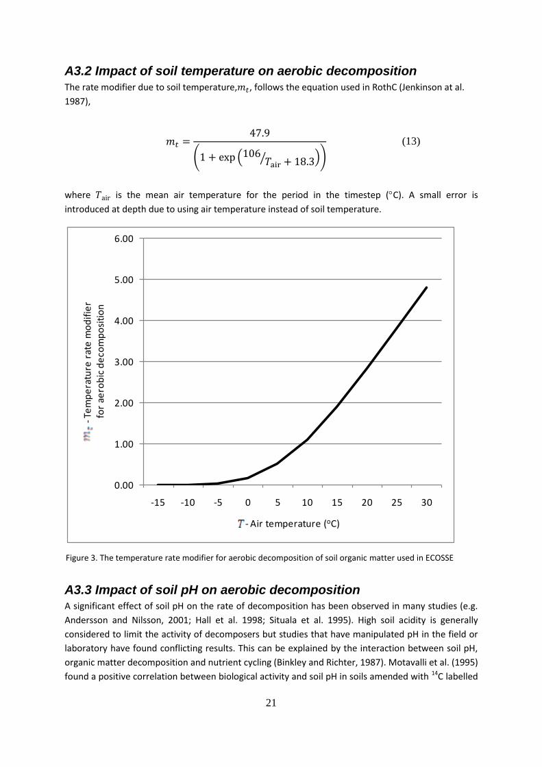
A3.2 Impact of soil temperature on aerobic decomposition

The rate modifier due to soil temperature, , follows the equation used in RothC (Jenkinson at al.

1987),

where is the mean air temperature for the period in the timestep (C). A small error is

introduced at depth due to using air temperature instead of soil temperature.

A3.3 Impact of soil pH on aerobic decomposition

A significant effect of soil pH on the rate of decomposition has been observed in many studies (e.g.

Andersson and Nilsson, 2001; Hall et al. 1998; Situala et al. 1995). High soil acidity is generally

considered to limit the activity of decomposers but studies that have manipulated pH in the field or

laboratory have found conflicting results. This can be explained by the interaction between soil pH,

organic matter decomposition and nutrient cycling (Binkley and Richter, 1987). Motavalli et al. (1995)

found a positive correlation between biological activity and soil pH in soils amended with 14C labelled

0.00

1.00

2.00

3.00

4.00

5.00

6.00

-15 -10 -5 0 5 10 15 20 25 30

-Te

mp

era

ture

rat

e m

od

ifie

rfo

r ae

rob

ic d

eco

mp

osi

tio

n

- Air temperature (oC)

(13)

Figure 3. The temperature rate modifier for aerobic decomposition of soil organic matter used in ECOSSE

22

plant residues. Similarly, Sitaula et al. (1995) used acid irrigation to examine the effect of low pH and

reported that pH 3 produced CO2 fluxes 20 % lower than at pH 4 and 5.5, between which there was

no significant difference. Persson and Wiren (1989) reported that increasing the acidity of forest soil

from pH 3.8 to 3.4 reduced CO2 evolution by 83 % and from pH 4.8 to 4 by 78 %.

These effects differ with redox conditions. Increases in pH have been reported to increase CO2

production 1.4-fold under anaerobic conditions but decrease it by 53 % under aerobic conditions

(Bridgham and Richardson, 1992). Bergman et al. (1999) compared CO2 production rates at pH 4.3

and 6.2, and found that under anaerobic conditions rates were 21 (at 7 C) and 29 (at 17 C) times

greater at the more neutral pH, while under aerobic conditions rates were 3 times greater at 7 C but

pH had no significant effect at 17 C.

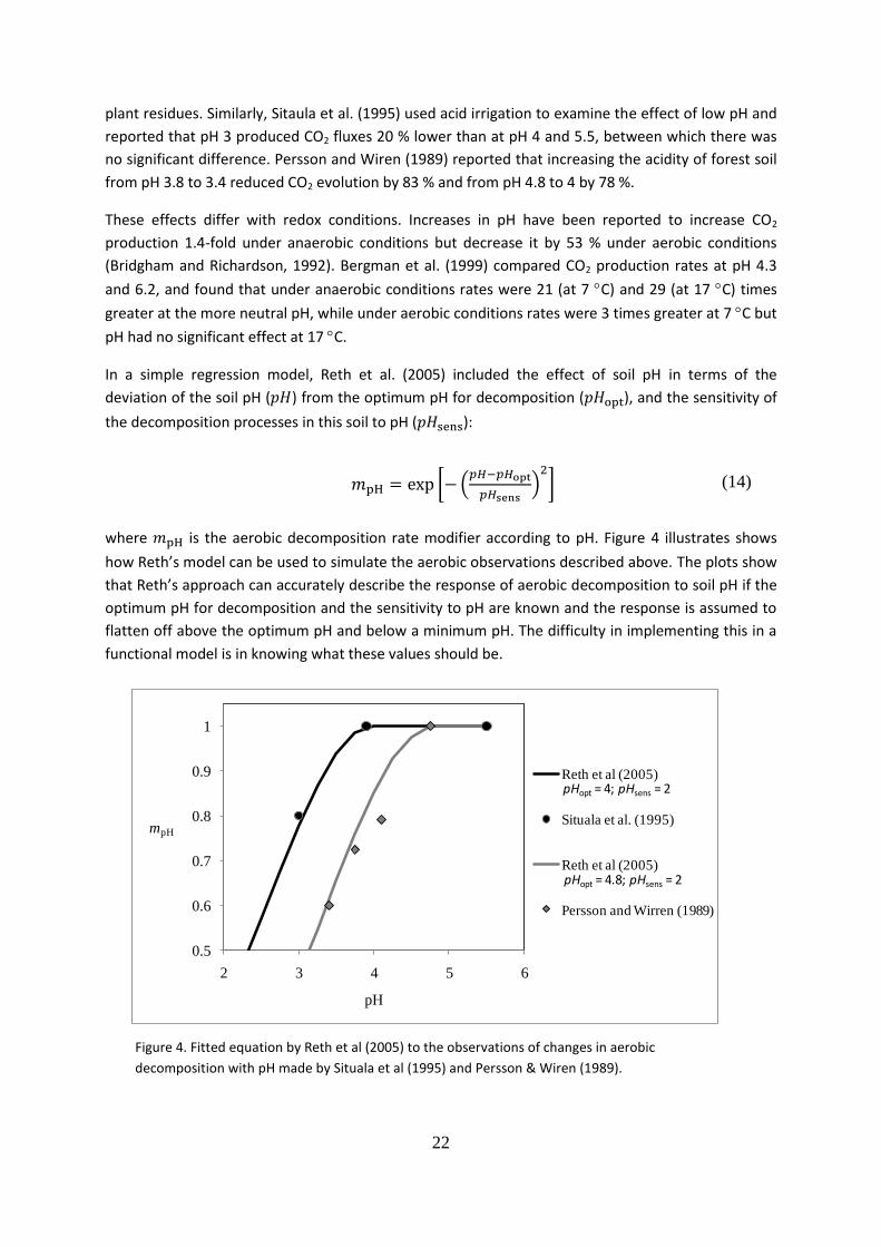
In a simple regression model, Reth et al. (2005) included the effect of soil pH in terms of the

deviation of the soil pH ( ) from the optimum pH for decomposition ( ), and the sensitivity of

the decomposition processes in this soil to pH ( ):

where is the aerobic decomposition rate modifier according to pH. Figure 4 illustrates shows

how Reth’s model can be used to simulate the aerobic observations described above. The plots show

that Reth’s approach can accurately describe the response of aerobic decomposition to soil pH if the

optimum pH for decomposition and the sensitivity to pH are known and the response is assumed to

flatten off above the optimum pH and below a minimum pH. The difficulty in implementing this in a

functional model is in knowing what these values should be.

0.5

0.6

0.7

0.8

0.9

1

2 3 4 5 6

mpH

pH

Reth et al (2005)

Situala et al. (1995)

Reth et al (2005)

Persson and Wirren (1989)

pHopt = 4; pHsens = 2

pHopt = 4.8; pHsens = 2

Figure 4. Fitted equation by Reth et al (2005) to the observations of changes in aerobic

decomposition with pH made by Situala et al (1995) and Persson & Wiren (1989).

(14)

23

The influence of soil pH on decomposition is not implemented in the SUNDIAL or RothC models as

they were originally designed to work in well-managed arable soils, and so it could be assumed that

the pH was close to neutral (Bradbury et al, 1993; Coleman and Jenkinson, 1996). This assumption

breaks down in natural and managed highly organic soils, where the pH is more variable. The above

discussion suggests that the implementation of decomposition in ECOSSE should include a different

description of the effects of pH on aerobic and anaerobic decomposition. In an approach that follows

that of Reth et al. (2005), but with a simplified formula that uses more explicit terms, aerobic

decomposition is described as proceeding at an optimum rate (rate modifier = 1) until the pH

falls below a critical threshold ( ), after which the rate of decomposition falls to a minimum

rate (rate modifier = ) at

This relationship is shown in Fig. 5. The values of , and can be set for each site,

but by default are set at = 0.2, = 1 and = 4.5 as these are the values that most

consistently simulate the observations described above.

A3.4 Impact of crop cover on aerobic decomposition

Following work by Jenkinson (1977) on the impact of plant cover on the decomposition of 14C

labelled ryegrass, the rate of decomposition is slowed using a crop cover rate modifier ( ) of 0.6 if

plants are actively growing, and 1 if the soil is bare.

(15)

0.5

0.6

0.7

0.8

0.9

1

2 3 4 5 6

mpH

pH

ECOSSE

Situala et al. (1995)

ECOSSE

Persson and Wirren (1989)

mpH,min = 0.2;pHmin = 0.5; pHmax = 4

mpH,min = 0.2;pHmin = 2; pHmax = 5

Figure 5. Anaerobic decomposition rate modifier for pH, , where = minimum

value for rate modifier according to pH; = pH at which rate of aerobic decomposition

is at minimum rate; and = Critical threshold pH below which rate of aerobic

decomposition starts to decrease

24

A3.5 Impact of nitrogen on aerobic decomposition

Following the approach used in the SUNDIAL model (Bradbury et al, 1993), N impacts the rate of

aerobic decomposition through the stable C:N ratio of the BIO and HUM pools. When organic matter

is added to the soil, the decomposition process is assumed to immobilise or mineralise N in order to

maintain the stable C:N ratio. If the C:N ratio of the added plant material is lower than the stable C:N

ratio, then sufficient N is released during the decomposition process to maintain the BIO and HUM

pools at the stable C:N ratio. If the C:N ratio of the added plant material is higher than the stable C:N

ratio then N is immobilised, first from the NH4+ pool, and then when that falls to a critical minimum

level defined for the soil, from the NO3- pool. If N in the NO3

- pool falls to the critical minimum level,

decomposition is limited to the amount of decomposition that can be achieved while maintaining the

BIO and HUM pools at the stable C:N ratio given the available mineral N.

ECOSSE differs from SUNDIAL in that it includes a variable efficiency of decomposition under N

limited conditions. The micro-organisms responsible for aerobic decomposition use SOM as a source

of energy, and to provide the C that is used to build biological structures. It is the amount of energy

required to drive these biological processes that determines the proportion of the decomposed

organic material that is retained in the soil, the efficiency of decomposition.

In N limited forest soils, it has been observed that decomposition can continue, even under N limited

conditions. When N is supplied to the system, for example as fertiliser, the C content of the soil

appears to increase relative to the C content of the N limited soil. It is hypothesized that this is in part

due to the microorganisms “mining” the SOM for N when N is limiting, emitting the excess C as CO2

and using the remaining N to build cell structures. When N becomes available, the micro-organisms

are no longer starved of N, so can use the energetically more accessible source of N, ammonium or

nitrate, rather than breaking down the SOM. This is simulated in ECOSSE by including a change to the

efficiency of decomposition ( ), described by the proportions of decomposing material retained as

biomass and humus. The efficiency of decomposition is allowed to be reduced by as much as is

required to ensure that there is sufficient available soil N to balance the C released into the BIO and

HUM pools. The efficiency of decomposition clearly has a lower limit of 0; indicating all of the

decomposed C will be released as CO2. The remaining N from the decomposing organic material is

released into the soil as ammonium. If the N required for decomposition is still higher than is

available from the SOM, then the rate of decomposition will be limited.

Change in pH has also been observed to result in a change in the C:N ratio of the organic matter in

the soil. The stable C:N ratio is an important driver of mineralization or immobilisation of N during

the decomposition of organic matter. In SUNDIAL, the stable C:N ratio of SOM is assumed to be a

constant value of 8 under all conditions (Bradbury et al. 1987). The choice of a stable C:N ratio of 8 is

a result of the weighted average of the C:N ratios of the decomposing fungi and bacteria in the soil.

However, as the soil pH falls, the ratio of fungi to bacteria increases because fungi are more tolerant

of acidic conditions. Because the C:N ratio of fungi is higher than the C:N ratio of bacteria, this

change in the population is accompanied by an increase in the stable C:N ratio of the SOM. This is

due to the decomposer community in the soil becoming dominated by fungi with a higher C:N ratio

than bacteria. This suggests that the stable C:N ratio of the organic matter pools in ECOSSE should

change with changing pH. In the absence of more detailed experimental data, a simple linear

approach is used.

25

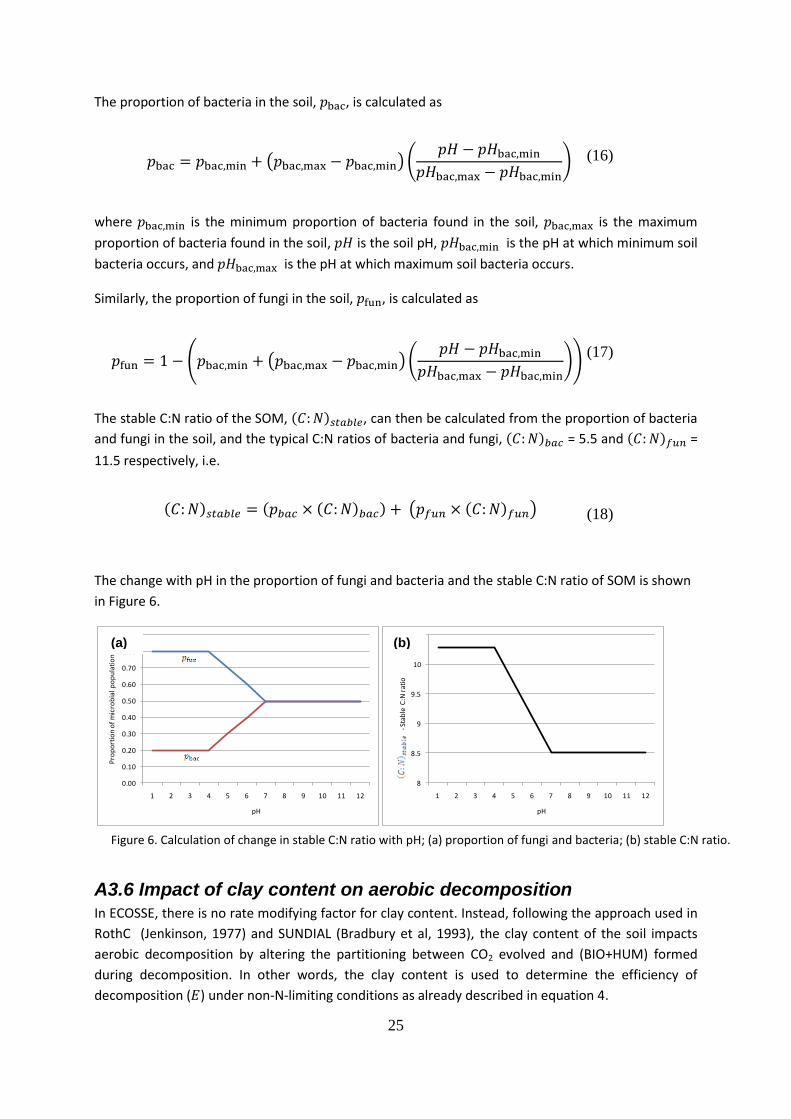
The proportion of bacteria in the soil, , is calculated as

where is the minimum proportion of bacteria found in the soil, is the maximum

proportion of bacteria found in the soil, is the soil pH, is the pH at which minimum soil

bacteria occurs, and is the pH at which maximum soil bacteria occurs.

Similarly, the proportion of fungi in the soil, , is calculated as

The stable C:N ratio of the SOM, , can then be calculated from the proportion of bacteria

and fungi in the soil, and the typical C:N ratios of bacteria and fungi, = 5.5 and =

11.5 respectively, i.e.

The change with pH in the proportion of fungi and bacteria and the stable C:N ratio of SOM is shown

in Figure 6.

A3.6 Impact of clay content on aerobic decomposition

In ECOSSE, there is no rate modifying factor for clay content. Instead, following the approach used in

RothC (Jenkinson, 1977) and SUNDIAL (Bradbury et al, 1993), the clay content of the soil impacts

aerobic decomposition by altering the partitioning between CO2 evolved and (BIO+HUM) formed

during decomposition. In other words, the clay content is used to determine the efficiency of

decomposition ( ) under non-N-limiting conditions as already described in equation 4.

0.00

0.10

0.20

0.30

0.40

0.50

0.60

0.70

0.80

0.90

1 2 3 4 5 6 7 8 9 10 11 12

Pro

po

rtio

n o

f m

icro

bia

l p

op

ula

tio

n

pH

8

8.5

9

9.5

10

10.5

1 2 3 4 5 6 7 8 9 10 11 12

-Sta

ble

C:N

rat

io

pH

(18)

(17)

(16)

Figure 6. Calculation of change in stable C:N ratio with pH; (a) proportion of fungi and bacteria; (b) stable C:N ratio.

(a)

(b)

26

A3.7 Evaluation of ECOSSE simulations of aerobic decomposition

An evaluation of the ECOSSE simulations of aerobic decomposition has been completed for a range

of soil conditions, in a number of different soil environments and under different land uses. This work

is currently being prepared for publication and so cannot be included here. When published, a

summary of the evaluation and a reference to the published paper will be provided.

A4 Anaerobic decomposition of soil organic matter pools

The process of anaerobic decomposition is included in the ECOSSE model, and is assumed to result in

emissions of CH4. Methane is an important contributor to global warming, which is produced by

methanogenic bacteria in soil when decomposition occurs under anaerobic, reducing conditions.

Wetlands represent the most important natural source of methane emissions to the environment.

The rate of methane emissions are often reported to increase with temperature, so there is potential

for positive feedback due to climate change. This emphasises the need to understand the processes

that control CH4 emissions from wetlands and how they react to both environmental and land use

changes.

The DNDC model (Zhang et al 2002) calculates CH4 production as a function of DOC concentration

and temperature, under anaerobic conditions where the soil redox potential (Eh) is predicted to be

150 mV or less. Methane oxidation is calculated as a function of soil CH4 and Eh. Methane moves

from anaerobic production zones to aerobic oxidation zones via diffusion, which is modelled using

concentration gradients between soil layers, temperature and soil porosity. Methane flux via plant

transport is a function of CH4 concentration and plant aerenchyma. The density of plant aerenchyma

is a function of the plant growth index, which is calculated using plant age and season days. If the

density of plant aerenchyma is not well developed, or soil is non-vegetated, the efflux is determined

by ebullition (bubbling). In DNDC, this is assumed to occur only at the surface level, and is regulated

by CH4 concentration, temperature, porosity, and any existing plant aerenchyma.

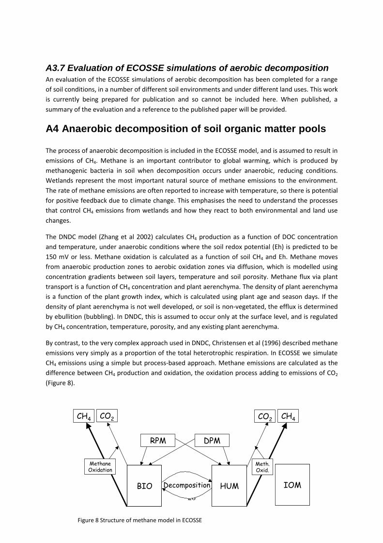
By contrast, to the very complex approach used in DNDC, Christensen et al (1996) described methane

emissions very simply as a proportion of the total heterotrophic respiration. In ECOSSE we simulate

CH4 emissions using a simple but process-based approach. Methane emissions are calculated as the

difference between CH4 production and oxidation, the oxidation process adding to emissions of CO2

(Figure 8).

CH4 CH4

Decomposition

CO2 CO2

DPMRPM

Meth.Oxid.

MethaneOxidation

BIO HUM IOMBIO HUM IOM

Figure 8 Structure of methane model in ECOSSE

27

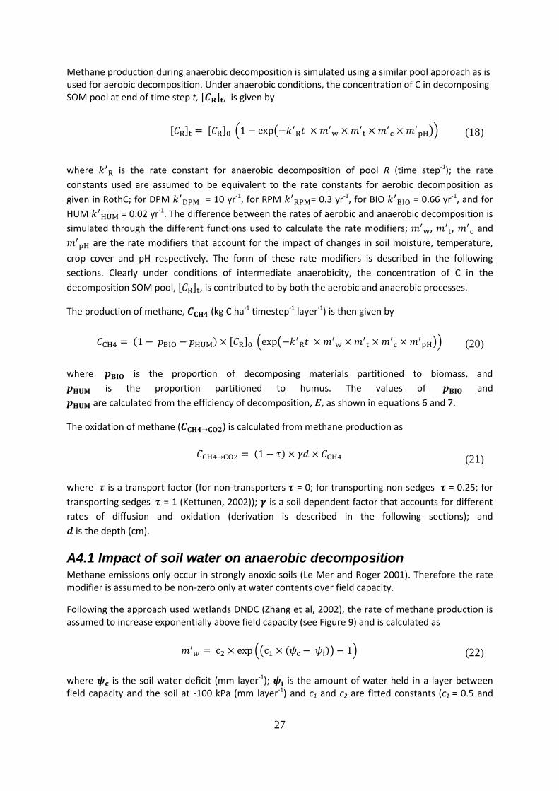
Methane production during anaerobic decomposition is simulated using a similar pool approach as is used for aerobic decomposition. Under anaerobic conditions, the concentration of C in decomposing SOM pool at end of time step t, , is given by

where is the rate constant for anaerobic decomposition of pool R (time step-1); the rate

constants used are assumed to be equivalent to the rate constants for aerobic decomposition as

given in RothC; for DPM = 10 yr-1, for RPM = 0.3 yr-1, for BIO = 0.66 yr-1, and for

HUM = 0.02 yr-1. The difference between the rates of aerobic and anaerobic decomposition is

simulated through the different functions used to calculate the rate modifiers; ,

, and

are the rate modifiers that account for the impact of changes in soil moisture, temperature,

crop cover and pH respectively. The form of these rate modifiers is described in the following

sections. Clearly under conditions of intermediate anaerobicity, the concentration of C in the

decomposition SOM pool, , is contributed to by both the aerobic and anaerobic processes.

The production of methane, (kg C ha-1 timestep-1 layer-1) is then given by

where is the proportion of decomposing materials partitioned to biomass, and is the proportion partitioned to humus. The values of and are calculated from the efficiency of decomposition, , as shown in equations 6 and 7.

The oxidation of methane ( ) is calculated from methane production as

where is a transport factor (for non-transporters = 0; for transporting non-sedges = 0.25; for

transporting sedges = 1 (Kettunen, 2002)); is a soil dependent factor that accounts for different

rates of diffusion and oxidation (derivation is described in the following sections); and is the depth (cm).

A4.1 Impact of soil water on anaerobic decomposition

Methane emissions only occur in strongly anoxic soils (Le Mer and Roger 2001). Therefore the rate modifier is assumed to be non-zero only at water contents over field capacity.

Following the approach used wetlands DNDC (Zhang et al, 2002), the rate of methane production is assumed to increase exponentially above field capacity (see Figure 9) and is calculated as

where is the soil water deficit (mm layer-1); is the amount of water held in a layer between field capacity and the soil at -100 kPa (mm layer-1) and c1 and c2 are fitted constants (c1 = 0.5 and

(22)

(21)

(20)

(18)

28

(where is the amount of water held in a layer between saturation and

the permanent wilting point (mm layer-1)). The rate modifier is shown in figure 8.

A4.2 Impact of soil temperature on anaerobic decomposition Field measurements of changes in methane emissions with temperature can be difficult to unravel,

as many confounding factors can contribute to the observed emissions. Christensen et al (2002)

report that mean seasonal temperature is the best predictor of methane fluxes on a large scale.

Hargreaves et al (2001) observed an exponential relationship between surface temperature (0-10

cm) and methane flux for measurements without a thaw period, with a Q10 of 4, while Rask et al

(2002) found a linear relationship between the same factors in a shallow bay area of a fen.

Hargreaves & Fowler (1998) reported a linear relationship with temperature between 7 and 11C,

with a slope of 5 μmol CH4 m-2 h-1 C-1 for peat wetlands in Caithness, Scotland. Other workers have

also reported significant relationships between soil temperature in the surface layer and methane

flux, in wet tundra sites (Christensen et al, 1995) and subalpine wetlands (Wickland et al, 1999,

2001). Although these field observations describe different responses, a positive relationship

between methane emissions and temperature is generally observed (Figure 10).

0

0.2

0.4

0.6

0.8

1

FieldCapacity

Available Water (mm)

Rate

Modif

ier,

m///w

ate

r

Saturation

Figure 9 Response of anaerobic decomposition to available

water in the soil

29

Micro- and mesocosm measurements provide a less complex picture, allowing confounding factors to

be removed from the experimental setup. Daulat & Clymo (1998) reported an exponential

relationship between soil temperature at 5 cm depth and mean methane flux in peat cores from

Scotland. Lloyd et al (1998) commented on the high sensitivity of methane fluxes from Scottish peat

cores to temperature, reporting a Q10 of 3 in the dark. MacDonald et al (1998) also report Q10 values

of around 3 (between 5 and 15oC) for relationships between peat temperature and methane flux

from peat cores from Northern Scotland, which are linear under semi-natural conditions, and

exponential under controlled conditions of constant humidity and light.

Following the model of Kettunen (2002), the temperature rate modifier is given by the equation:

where is the temperature of the soil layer (C) In agreement with the observations of Daulat & Clymo (1998), Lloyd et al. (1998) and MacDonald et al. (1998), this relationship shows a Q10 value close to 3 between 5 and

15C (see Fig. 11).

(23)

0

1

2

3

4

5

6

-5 0 5 10 15 20 25 30 35 40

Soil Temperature (oC)

Rate

Modifi

er

for

Tem

pera

ture

(m

/// te

mp)

.

Q10 = 3

Figure 11 Response of anaerobic decomposition to soil

temperature

0

2000

4000

6000

8000

10000

12000

14000

16000

0 2 4 6 8 10 12 14 16Temperature

CH

4 u

g/m

2/h

Hargreaves et al, 2001Rask et al, 2002Daulat & Clymo, 1998MacDonald et al, 1998 (semi-natural)Hargeaves & Fowler, 1998

Figure 10 Reported responses of methane emissions to temperature

30

A4.3 Impact of soil pH on anaerobic decomposition

Methanogenic bacteria are generally reported to exhibit maximum activity under neutral or slightly

higher pH conditions (Garcia et al, 2000) and to be very sensitive to variations in soil pH (Wang et al,

1993). Garcia et al (2000) reported that 68 species of methanogenic bacteria could not grow at a pH

lower than 5.6. However, methane producers can adapt to more acidic environments, as many

studies have recorded methanogenic activity in soils with a lower pH. Williams and Crawford (1985)

reported that a mixed bacterial culture from a Minnesota peatland produced methane at pH values

between 3 and 4. Dunfield et al (1993) investigated methane production in peat soil samples from

temperate and subarctic areas (pH 3.5–6.3) and reported an optimum production rates at pH of 5.5

to 7.0. Inubushi et al (2005) reported a positive correlation between methane production activity and

soil pH (r2 = 0.802, P <0.01) for peat soil samples from a temperate Japanese wetland, which had a

pH range of 5-7. However, more acidic Indonesian peat soils, which ranged from pH 3.9-5, showed no

correlation with pH (Inubushi et al, 2005). Depth can also affect the influence of soil pH on methane

production. Williams and Crawford (1984) found that a pH increase from 3.2 to 5.8 increased the

methane production of an incubated peat from a Minnesota peatland by 1.5 fold, for samples from

10 cm depth, and 2.2 fold for samples from 60 cm depth. To complicate things further, some studies

have reported negative relationships. Bergman et al (1999) reported a negative effect of pH on

methane production in incubations of peat soil from a Swedish mire, but it was only statistically

significant for one of two years data. Bergman et al (1999) reported both positive and negative

relationships with pH for peat originating from different plant communities within the same mixed

mire site in Sweden, and suggested that conflicting results may be due to competition for hydrogen

between methanogens and homoacetogens, increasing pH favouring the later since it increases the

degree of dissociation of acetate, or due to differences in cation exchange capacity (CEC).

It is clear that the response of methane

production to pH is very complex. Some

of these conflicting results may have been

confounded by methane oxidation.

However, from the above results it can be

stated that the rate of methane

production is usually at an optimum (m/pH

= 1) at around pH 7 (Garcia et al, 2000;

Wang et al, 1993), and is close to the

optimum between pH 5.5 –7 (Dunfield et

al., 1993), decreasing to close to zero at

around pH 3 (Williams & Crawford, 1984,

1985; Dunfield et al., 1993). This response

can be simulated using a sigmoid

relationship),

where is the measured pH of the soil layer, and and are constants ( = -1, and = -50).

The relationship between and is shown in Fig. 12.

(24)

0

0.1

0.2

0.3

0.4

0.5

0.6

0.7

0.8

0.9

1

2 2.5 3 3.5 4 4.5 5 5.5 6 6.5 7 7.5 8 8.5 9

Soil pH

Rate

Modifi

er

for

pH

(m

/// p

H)

.

Figure 12. Response of anaerobic decomposition to soil pH

31

A4.4 Impact of crop cover on anaerobic decomposition

Anaerobic decomposition is assumed to follow the same response to crop cover as used for aerobic

decomposition.

A4.5 Impact of nitrogen on anaerobic decomposition

Nitrogen is assumed to have the same impact on anaerobic decomposition as it does on aerobic

decomposition.

A4.6 Impact of clay content on anaerobic decomposition

As for aerobic decomposition, the clay content of the soil impacts aerobic decomposition by altering

the partitioning between CO2 evolved and (BIO+HUM) formed during decomposition.

A4.7 Impact of oxygen on methane emissions

Water table depth is one of the main factors controlling methane emissions as it determines the

position of the boundary between the anaerobic and aerobic zones. When the water table is below

the soil surface, oxidation of methane becomes a major controlling variable for methane efflux

(Christensen et al, 2000). As a result, a lower water table decreases methane emission (Blodau et al,

2004) and draining peats may even convert the soil to a net methane sink (Blodau & Moore, 2003;

Huttunen et al, 2003; Maljanen et al, 2002). Hargreaves & Fowler (1998) measured methane fluxes

over a peat wetland in Caithness and related them to water table depths in different areas of the

bog. They found a negative

linear relationship between

depths of around 8-17 cm.

Daulat & Clymo (1998) also

report a linear relationship

between water table depth

and methane emission, with

depths of more than 15-20 cm

below the soil surface stopping

peat cores from being a net

emitter of methane (Fig. 13).

MacDonald et al (1998) found

a reduction in methane

emissions from Scottish peat

cores with increasing water table depth, but in this case, the observed relationship is a decay curve

and the cores do not become net sinks for methane even when the water table is 40 cm below the

surface. Moore & Dalva (1993) found a negative logarithmic correlation with water table depth,

down to 60 cm, in cores of peatland. Where the water table is above the surface, oxidation can also

reduce methane emissions, particularly if light availability allows benthic photosynthetic activity (Le

Mer & Roger, 2001).

If it can be assumed that methane oxidation is close to zero when the water table is at the surface,

the soil factor accounting for diffusion and oxidation of methane ( ) can be calculated from the

-200

0

200

400

600

800

1000

0 5 10 15 20 25

Water table depth (cm)

CH

4 (

ug

/m2/h

)

Daulat & Clymo 1998

Daulat & Clymo 2

Daulat & Clymo 3

Hargreaves & Fowler,

1998

Figure 13. Reported responses of methane emissions to water

table depth

32

depth (in cm) at which methane emissions cease and the soil becomes a net methane sink ( ) as

follows:

This results in a value of =

0.056 cm-1 for the soils of

Daulat and Clymo (1998), and

= 0.04 cm-1 for the soils of

Hargreaves and Fowler

(1998). The methane

emissions calculated in this

way are shown in Fig. 14.

Further work is required to

determine the relationship

between soil type and the

depth at which the soil

becomes a net methane sink.

Methane oxidizing bacteria

(methanotrophs) are more tolerant to pH variations than methanogens, with a reported optimum pH

of 5.0 to 6.5 in temperate and subarctic peats (Dunfield et al, 1993), and have been discovered in

peat soils below pH 4.7 using molecular ecological methods (MacDonald et al, 1996). However,

Hutsch et al (1994) reported that, in a non-fertilised permanent grassland at the Rothamsted

experimental station, a decrease in pH from 6.3 to 5.6 reduced methanotrophy by almost half. As a

first approximation, it is assumed that methane oxidation is not influenced by soil pH.

A4.8 Evaluation of ECOSSE simulations of anaerobic decomposition An evaluation of the ECOSSE simulations of anaerobic decomposition has been completed for a range

of soil conditions, in a number of different soil environments and under different land uses. This work

is currently being prepared for publication and so cannot be included here. When published, a


A5 Nitrogen transformations

A5.1 Mineralisation / Immobilisation As already described in section A3.5, mineralisation / immobilisation turnover is calculated following

the approach used in the SUNDIAL model by Bradbury et al (1993), modified to allow for N limited

conditions.

A5.2 Nitrification

DNDC predicts nitrification rates by tracking nitrifier activity and NH4+ concentration. Growth and

death rates of nitrifying bacteria are calculated as a function of DOC concentration, temperature and

(25)

-200

0

200

400

600

800

1000

0 5 10 15 20 25

Water Table Depth (cm)

CH

4 u

g m

-2 h

-1

Daulat & Clymo 1998 Hargreaves & Fowler, 1998

Figure 14. Reduction in methane emissions with depth of water

table, as calculated by ECOSSE

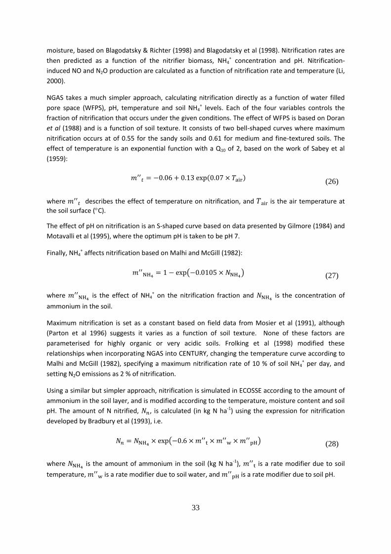
33

moisture, based on Blagodatsky & Richter (1998) and Blagodatsky et al (1998). Nitrification rates are

then predicted as a function of the nitrifier biomass, NH4+ concentration and pH. Nitrification-

induced NO and N2O production are calculated as a function of nitrification rate and temperature (Li,

2000).

NGAS takes a much simpler approach, calculating nitrification directly as a function of water filled

pore space (WFPS), pH, temperature and soil NH4+ levels. Each of the four variables controls the

fraction of nitrification that occurs under the given conditions. The effect of WFPS is based on Doran

et al (1988) and is a function of soil texture. It consists of two bell-shaped curves where maximum

nitrification occurs at of 0.55 for the sandy soils and 0.61 for medium and fine-textured soils. The

effect of temperature is an exponential function with a Q10 of 2, based on the work of Sabey et al

(1959):

where describes the effect of temperature on nitrification, and is the air temperature at

the soil surface (C).

The effect of pH on nitrification is an S-shaped curve based on data presented by Gilmore (1984) and

Motavalli et al (1995), where the optimum pH is taken to be pH 7.

Finally, NH4+ affects nitrification based on Malhi and McGill (1982):

where is the effect of NH4

+ on the nitrification fraction and is the concentration of

ammonium in the soil.

Maximum nitrification is set as a constant based on field data from Mosier et al (1991), although

(Parton et al 1996) suggests it varies as a function of soil texture. None of these factors are

parameterised for highly organic or very acidic soils. Frolking et al (1998) modified these

relationships when incorporating NGAS into CENTURY, changing the temperature curve according to

Malhi and McGill (1982), specifying a maximum nitrification rate of 10 % of soil NH4+ per day, and

setting N2O emissions as 2 % of nitrification.

Using a similar but simpler approach, nitrification is simulated in ECOSSE according to the amount of

ammonium in the soil layer, and is modified according to the temperature, moisture content and soil

pH. The amount of N nitrified, , is calculated (in kg N ha-1) using the expression for nitrification

developed by Bradbury et al (1993), i.e.

where is the amount of ammonium in the soil (kg N ha-1), is a rate modifier due to soil

temperature, is a rate modifier due to soil water, and

is a rate modifier due to soil pH.

(28)

(27)

(26)

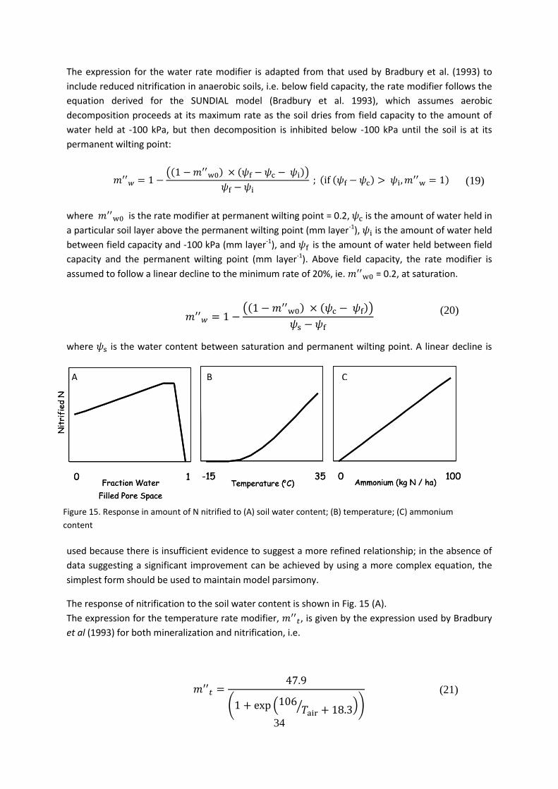
34

The expression for the water rate modifier is adapted from that used by Bradbury et al. (1993) to

include reduced nitrification in anaerobic soils, i.e. below field capacity, the rate modifier follows the

equation derived for the SUNDIAL model (Bradbury et al. 1993), which assumes aerobic

decomposition proceeds at its maximum rate as the soil dries from field capacity to the amount of

water held at -100 kPa, but then decomposition is inhibited below -100 kPa until the soil is at its

permanent wilting point:

where is the rate modifier at permanent wilting point = 0.2, is the amount of water held in

a particular soil layer above the permanent wilting point (mm layer-1), is the amount of water held

between field capacity and -100 kPa (mm layer-1), and is the amount of water held between field

capacity and the permanent wilting point (mm layer-1). Above field capacity, the rate modifier is

assumed to follow a linear decline to the minimum rate of 20%, ie. = 0.2, at saturation.

where is the water content between saturation and permanent wilting point. A linear decline is

used because there is insufficient evidence to suggest a more refined relationship; in the absence of

data suggesting a significant improvement can be achieved by using a more complex equation, the

simplest form should be used to maintain model parsimony.

The response of nitrification to the soil water content is shown in Fig. 15 (A).

The expression for the temperature rate modifier, , is given by the expression used by Bradbury

et al (1993) for both mineralization and nitrification, i.e.

0 1Fraction Water

Filled Pore Space

Nit

rifi

ed N

-15 35Temperature (oC)

0 100Ammonium (kg N / ha)

0 1Fraction Water

Filled Pore Space

Nit

rifi

ed N

-15 35Temperature (oC)

0 100Ammonium (kg N / ha)

Figure 15. Response in amount of N nitrified to (A) soil water content; (B) temperature; (C) ammonium

content

A B C

(19)

(20)

(21)

35

where is the air temperature (°C).

The response to air temperature is shown in Fig. 15 (B), and the response to ammonium is shown in

Fig. 15 (C).

The pH response function suggested by Parton et al (1996) was used. In this model, rate is about 1

(unmodified) at about neutral pH, but decreases below neutral:

Conversion of ammonium to nitrate by nitrification is

accompanied by gaseous losses of N due to complete and

partial nitrification. The gaseous losses as NO and N2O are

calculated using linear relationships shown in Fig. 16.

The amount of gas emitted as N2O during nitrification,

, is given (in kg N ha-1) by

where = 0.2 is the proportion of N2O produced due to partial nitrification at field capacity, =

0.02 is the proportion of full nitrification lost as gas, and = 0.1 is the proportion of full

nitrification gaseous loss that is NO.

Similarly, the amount of gas emitted as NO during nitrification, Nn,NO is given (in kg N ha-1) by

A5.3 Denitrification Denitrification is a process that responds to changes in the system on a shorter timescale than many

of the other C and N turnover processes. As a result, denitrification is difficult to measure accurately,

and difficult to simulate without short-term and detailed input data. As a result, many models of

0 1Fractiion Water

Filled Pore Space

Gas

eou

s N

Los

s N2O produced by nitrification

NO produced by nitrification

N2O produced by partial

nitrification

0 1Fractiion Water

Filled Pore Space

Gas

eou

s N

Los

s N2O produced by nitrification

NO produced by nitrification

N2O produced by partial

nitrification

Figure 16. Partitioning of N lost by

denitrification into N2 and N2O with respect to

soil water and nitrate content

(22)

(23)

(24)

36

denitrification have high data requirements. The aim in ECOSSE is to develop a model that will

simulate processes to the required accuracy but without the need for detailed data that will not be

available at the large scale.

The denitrification sub-model of DNDC calculates N2O and NO production, consumption and diffusion

during rainfall, irrigation and flooding events. DNDC simulates relative growth rates of nitrate, nitrite,

NO, and N2O denitrifiers based on soil Eh, and concentration of DOC and N oxides. The soil matrix is

divided into aerobic and anaerobic zones using an "anaerobic balloon", which swells and shrinks in

response to oxygen diffusion and consumption in the soil profile. Substrates allocated to the

anaerobic zone of the profile are then used to determine the denitrifier growth rates based on a

simple function of multinutrient-dependent growth (based on Bader, 1978). The death rate is a

constant fraction of total denitrifier biomass. Relative growth rates for denitrifiers with different

substrates are assumed to be independent, and competition takes place via the common DOC

substrate (based on Leffelaar & Wessel, 1988). Substrate consumption rates are calculated using

growth rates and biomass. NO, N2O and N2 fluxes are calculated using the basic laws of kinetics, as

denitrification is a typical sequential reaction. As intermediates of the reactions, NO and N2O fluxes

are determined by rates of production, consumption and escape from the reacting system. Escape is

controlled by diffusion rate, a function of soil porosity, moisture, temperature and clay content (Li,

2000).

The CENTURY denitrification model in NGAS is based on data from Weier et al (1993). Total

denitrification N gas fluxes (N2 + N2O) are a function of soil heterotrophic respiration rate (index of

carbon availability), soil NO3- levels, and soil water filled pore space. Soil NO3

- levels and respiration

rate determine the maximum total N gas flux according to s-shaped curves fitted to experimental

data. This maximum is then reduced by a fraction determined by water filled pore space, as a

function of soil texture. Maximum denitrification occurs where water filled pore space is 0.9 or

above. Below this value, denitrification is reduced exponentially, with fine soils declining most

rapidly, followed by medium and then coarse soils. Denitrification drops to zero at water filled pore

space of 0.6 for fine soils, 0.5 for medium and 0.4 for coarse. Total denitrification N gas flux is then

partitioned into N2 and N2O as a function of soil NO3-, WFPS and soil respiration (Parton et al, 1996).

In ECOSSE, a simpler approach is used in which total denitrification is simulated as a proportion of

the nitrate content of the layer, modified according to water content and biological activity of the

soil (as described by CO2 release during decomposition). The denitrified N is then divided into N2, N2O

and NO according to the water and nitrate content of the soil The total loss of N due to

denitrification is given by

where is the amount of nitrogen emitted from the soil during denitrification (kg N ha-1);

modifies this amount depending on the nitrate level, depending on the water content, and

depending on the biological activity of the soil; and is the amount of nitrate in the soil (kg

N ha-1 layer-1).

(25)

37

The nitrate modifier, , is based on the model developed by Henault and Germon (2000), i.e.

.

The response of the denitrification process to the amount of nitrate in the soil is shown in Fig. 17 (A).

The water modifier, , is based on the fitted equation of Grundmann and Rolston (1987), i.e.

where is the calculated water content and is the field capacity maximum water content of the

soil (mm layer-1). The response of the denitrification process to the soil water content is shown in Fig.

17 (B).

The biological activity modifier, , is based on the relationship developed by Bradbury et al

(1993), i.e.

where is the amount of CO2 produced during mineralization (kg C ha-1 timestep-1). This acts as a

surrogate measure of the soil biological activity. The response of the denitrification process to the

soil biological activity is shown in Figure 17 (C).

The N lost by denitrification, , is partitioned into N2 and N2O using simple linear relationships

shown in Figure 18.

0 1Fraction Water

Filled Pore Space

Deni

trif

ied N

Carbon Dioxide

Production

Nitrate in soil 0 1

Fraction Water

Filled Pore Space

Deni

trif

ied N

Carbon Dioxide

Production

Nitrate in soil

Figure 17. Response in amount of N emitted due to denitrification to (A) nitrate in soil; (B) soil water

content; (C) biological activity

A B C

(26)

(27)

(28)

38

The amount of N2 gas lost by denitrification, , is given (in kg N ha-1) by

where is amount of N2 gas lost by denitrification (kg N ha-1), proportions denitrification into

N2 according to the water content of the soil, (

where = 0.5 is the proportion of

denitrified N lost as N2 at field capacity), and proportions denitrification into N2 according to the

nitrate content of the soil, (

where = 0.1 is the proportion

at which

N2 emission falls to zero and all denitrified N is lost as nitrate.

The amount of N2O gas lost by denitrification, , is similarly calculated (in kg N ha-1) by the

following expression,

A5.4 Nitrate leaching In SUNDIAL-MAGEC, the soil is divided into different layers for the different components of the soil:

ammonium is simulated in 50cm layers down the soil profile; SOM is simulated in 25cm layers to a

maximum depth of 50cm; and nitrate is simulated in 5cm layers for the top 50cm, followed by 50cm

layers for the remainder of the profile. This structure does not allow C and N turnover in deep

organic soils to be simulated. In ECOSSE, the layers are unified into 5cm layers throughout, so

allowing C and N turnover to be simulated to depth. The soil parameters are also described in 5cm

layers, so allowing more detailed descriptions of soil profile characteristics to be included. This is

important in highly organic soils where the organic layer can be very deep.

A5.5 Leaching of dissolved organic matter

Dissolved Organic Carbon (DOC) is a potentially important component of carbon export from the soil

system under highly organic conditions. Dissolved Organic Nitrogen (DON) is closely linked to the

0 1Fractiion Water

Filled Pore Space

Gas

eou

s N

Los

s N2O produced by denitrification

N2 produced by denitrification

0 100Nitrate (kg/ha)

N2O produced by denitrification


0 1Fractiion Water

Filled Pore Space

Gas

eou

s N

Los

s N2O produced by denitrification


0 100Nitrate (kg/ha)

N2O produced by denitrification


Figure 18. Partitioning of N lost by denitrification into N2 and N2O with respect to

soil water and nitrate content

(29)

(40)

39

production of DOC, and Jörgensen & Richter (1992) demonstrated that the two soil characteristics

must be considered together in order to avoid unrealistic simulations of carbon or nitrogen

concentration in the soil. Evans et al. (2005) give a convincing argument that DOC production in

organic soils is increasing, not due to climate change-induced oxidation, but instead as a result of

soils recovering from acid deposition, which suppresses DOC solubility. They demonstrate a link

between increased temperature, declining sulphur deposition and sea-salt loading. Strong links are

already known to exist between soil water pH and DOC solubility, with an inverse relationship

between mineral and organic acid export from soils (Krug and Frink, 1983). Palmer et al. (2001) used

a combination of stable isotope and 14C-dating to identify the main sources and processes controlling

DOC production in a temperate non-forested watershed underlain by mostly organic and podzolic

soils. They found that the main source of DOC was the readily-decomposable carbon, such as leaf

litter, rather than the longer term storage of SOM. They also showed that wetter soils export more

‘recent’ carbon than dry soils: DOC from dry soils contains more of the older carbon than does DOC

from wet soils.

DyDOC is a model of DOC production that utilises a layered soil description (Michalzik et al., 2003),

and contains different organic fractions. Three processes are represented in DyDOC: hydrology,

metabolism and sorption. Hydrology is modelled in terms of macropores and micropores, between

which dissolved organic carbon diffuses. Metabolism is modelled using relatively simple relationships

to define the transformations between the three pools of organic carbon, with only temperature

being a variable. Sorption occurs to and from soil solids from the different pools, and is controlled by

DOC type, soil solution pH and cation content, and the nature of the soil solids (texture etc.). In

ECOSSE, we follow a similar approach, simulating the hydrological, metabological and sorptive

processes using the 5 soil organic matter pools: decomposable and resistant plant material, soil

biomass, humus, and inert organic matter. A further organic matter pool is introduced, containing

the DOC and DON that is in solution (see Fig. 19).

This dissolved component is then susceptible to

leaching by the same processes as already exist in

the model to describe leaching losses. According to

the model of Aguilar & Thibodeaux (2005a; 2005b),

there are two fractions of DOC, one fraction that is

readily available in the soil solution at all times,

and another that is created from slower

decomposition processes. This observation is

consistent with the transfer into the DOC pool

during decomposition of material from the rapidly

turning over biomass and plant material pools, as

well as from the more slowly turning over humus

pool. In DyDOC production by metabolism is calculated using a Q10 relationship with a rate

dependent only on temperature:

DOC

BIOMASS

HUMUS

DPM

RPM

CO2

Figure 19. Pool structure for DOC production

and uptake

(41)

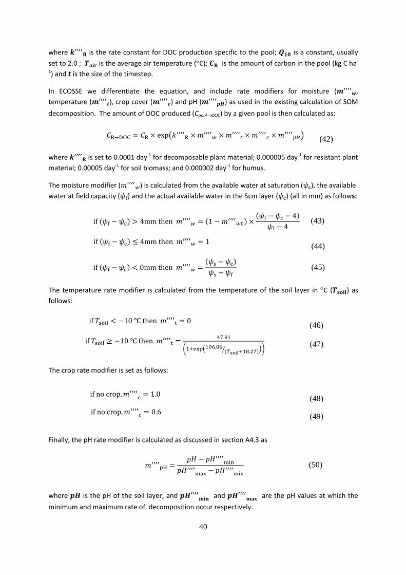
40

where is the rate constant for DOC production specific to the pool; is a constant, usually

set to 2.0 ; is the average air temperature (C); is the amount of carbon in the pool (kg C ha-

1) and is the size of the timestep.

In ECOSSE we differentiate the equation, and include rate modifiers for moisture ( ,

temperature ( ), crop cover (

) and pH ( ) as used in the existing calculation of SOM

decomposition. The amount of DOC produced (CpoolDOC) by a given pool is then calculated as:

where is set to 0.0001 day-1 for decomposable plant material; 0.000005 day-1 for resistant plant

material; 0.00005 day-1 for soil biomass; and 0.000002 day-1 for humus.

The moisture modifier ( ) is calculated from the available water at saturation ( ), the available

water at field capacity ( ) and the actual available water in the 5cm layer ( ) (all in mm) as follows:

The temperature rate modifier is calculated from the temperature of the soil layer in C ( ) as

follows:

The crop rate modifier is set as follows:

Finally, the pH rate modifier is calculated as discussed in section A4.3 as

where is the pH of the soil layer; and and

are the pH values at which the

minimum and maximum rate of decomposition occur respectively.

(42)

(43)

(44)

(45)

(46)

(47)

(48)

(49)

(50)

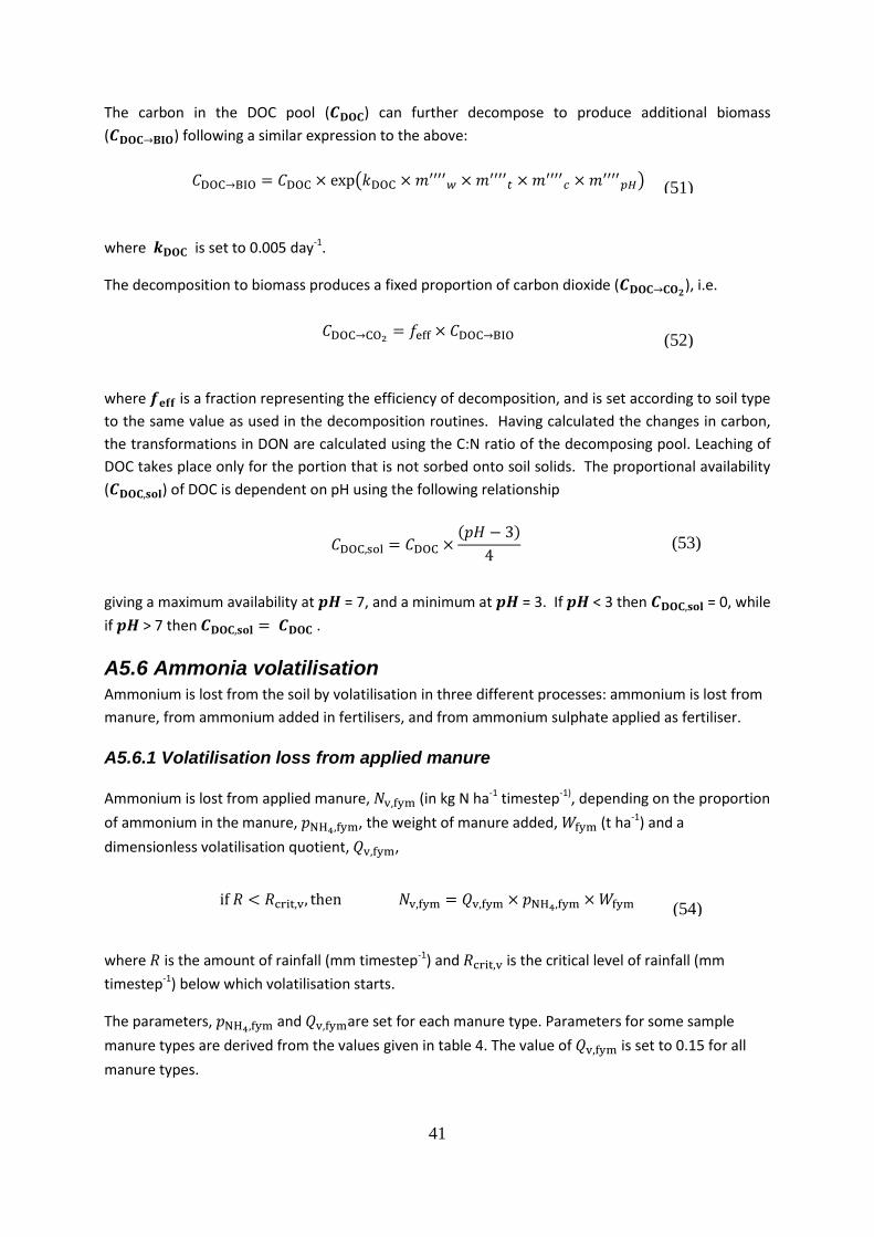
41

The carbon in the DOC pool ( ) can further decompose to produce additional biomass

( ) following a similar expression to the above:

where is set to 0.005 day-1.

The decomposition to biomass produces a fixed proportion of carbon dioxide ( ), i.e.

where is a fraction representing the efficiency of decomposition, and is set according to soil type

to the same value as used in the decomposition routines. Having calculated the changes in carbon,

the transformations in DON are calculated using the C:N ratio of the decomposing pool. Leaching of

DOC takes place only for the portion that is not sorbed onto soil solids. The proportional availability

( ) of DOC is dependent on pH using the following relationship

giving a maximum availability at = 7, and a minimum at = 3. If < 3 then = 0, while

if > 7 then .

A5.6 Ammonia volatilisation

Ammonium is lost from the soil by volatilisation in three different processes: ammonium is lost from

manure, from ammonium added in fertilisers, and from ammonium sulphate applied as fertiliser.

A5.6.1 Volatilisation loss from applied manure

Ammonium is lost from applied manure, (in kg N ha-1 timestep-1), depending on the proportion

of ammonium in the manure, , the weight of manure added, (t ha-1) and a

dimensionless volatilisation quotient, ,

where is the amount of rainfall (mm timestep-1) and is the critical level of rainfall (mm

timestep-1) below which volatilisation starts.

The parameters, and are set for each manure type. Parameters for some sample

manure types are derived from the values given in table 4. The value of is set to 0.15 for all

manure types.

(51)

(52)

(53)

(54)

42

Table 4.Parameters used to describe organic manures in ECOSSE

Manure Type

Dry

matter in fresh

manure

(t dry weight

(t fresh

man.)-1)

N in dry matter in

manure

(kg N (t dry

matter)-1)

C in dry matter in

manure

(kg C (t dry

matter)-1)

N in

manure that is

NH4+

(%)

Percent

of

manure that is

lost as

gas (%)

Critical level

of rainfall below which

volatilisation

occurs

N in manure that is

decomposed

organic matter

(%)

Percent of

manure

added in top 25cm

(%)

Liquid? (0=no;

1=yes)

Cattle FYM 25 2.4 21 20 25 5 10 100 0

Pig FYM 25 2.8 25 20 25 5 10 100 0

Layer Manure 30 5.0 32 50 30 5 25 100 0

Broiler/Turkey

Manure 60 4.8 30 50 30 5 35 100 0

Sewage

Sludge Cake

(Undigested)

25 3.0 25 20 25 5 35 100 0

Sewage Sludge Cake

(Digested)

25 3.0 25 15 25 5 35 100 0

Dairy Slurry 6 5.0 20 57 40 5 20 80 1

Beef Slurry 6 3.8 20 50 40 5 20 80 1

Pig Slurry 6 8.3 25 70 42 5 32 80 1

Strainer Box

Separated

Slurry

1.5 10.0 30 50 20 5 20 80 1

Weeping Wall Separated

Slurry

3 10.0 30 50 20 5 25 80 1

Mechanically

Separated

Slurry

4 10.0 30 50 20 5 20 80 1

Sewage Sludge Liquid

(Undigested)

5 3.6 25 45 40 5 15 80 1

Sewage

Sludge Liquid (Digested)

4 5.0 30 45 40 5 15 80 1

A5.6.2 Volatilisation loss from fertiliser

Ammonium is volatilised from urea and ammonium sulphate added as fertiliser as calculated by the

following equation:

where and are the volatilisation quotients for urea and ammonium sulphate, set to 0.15

for both, is the proportion of urea in the fertiliser, is the proportion of ammonium

sulphate in the fertiliser, and is the amount of fertiliser N applied (kg N ha-1 timestep-1).

(55)

43

A5.7 Crop nitrogen uptake

Nitrogen is taken up by the growing plant and C and N are returned to the soil by the plant following

the approach published by Bradbury et al (1993). The site specific version of the model requires

detailed information about management and is designed to be used with arable crops. ECOSSE has

been further developed to allow simulations when only limited data are available to describe the

growing conditions of the plants.

A5.7.1 Plant Inputs

If provided as an input, the total plant inputs of C ( ) are assumed to be given by the net primary

production. If the net primary production is entered as zero, the plant inputs are either calculated

from the initialisation described in A2.2 or estimated using the MIAMI model (Leith, 1972). The N

inputs from the plant to the soil ( ) are calculated using standard C:N ratios for the different

land uses,

The C:N ratios of simple land use classes, arable, grassland, forestry and semi-natural are initially all

set to 10.

As an alternative, in the site specific version of the model, the plant inputs of C and N can be

calculated from the expected yield as described by Bradbury et al (1993). The plant input of carbon

( is given by

where , , , and are empirical parameters, specific to each crop or plant

type, and is the crop yield (t ha-1) (moisture content used for the crop yield depends on the

crop type).

The plant input of nitrogen ( ) is calculated from the amount of N taken up in above ground plant

A5.7.2 Timing of Management Events

Management events are set using standard values for the different land use types. Arable crops are

assumed to be sown in February and harvested in October: all other land uses are assumed to stay in

the ground throughout the year. Arable and grassland are assumed to have fertiliser applied during

March: no other land uses have fertiliser applications. Initially, farmyard manure is assumed not to

be applied.

A.5.7.3 Fertiliser Applications

In the site specific version of the model, recorded fertiliser applications are entered by the user. In

the limited data or GIS version of the model, the fertiliser applications for arable crops are assumed

to meet the nitrogen requirement of the crop. This is a reasonable assumption, because if they did

not, then the plant would not grow and the calculated C inputs would not have been achieved. If

(56)

(57)

(58)

44

(62)

fertiliser applications had exceeded the requirements of the crop, the losses by leaching and

denitrification would have been greater than simulated. However, without further information on

application rates, this cannot be estimated. If it is assumed that the N returned to the soil is the total

N requirement less the N in the above ground parts of the plant at harvest, the total N requirement

can be derived from equations used in SUNDIAL for total N requirement and N in above ground plant

at harvest (Smith et al, 1996). Here, a typical arable crop has been taken to be a winter wheat crop

with a yield of 8 t ha-1 ( = 8). This is a good assumption for UK conditions, but can be changed if

a land use class is being derived for a differently yielding crop or for a country where winter wheat is

not the dominant arable crop. The total N input to the soil as crop debris ( ) is given in SUNDIAL

by

where is the proportion of N in above ground crop that is incorporated in the soil, is

the N in above ground, is the proportion of N in below ground crop that is incorporated in the

soil and is the N in below ground parts of the plant at harvest. For winter wheat is set

to 0.12 and is set to 1.0

The N in below ground parts of the plant at harvest ( ) are given by

where , and are empirical parameters describing the uptake of N in below ground parts

of the plant. For winter wheat, = 63, = -0.65 and = 1, so .

The N in above ground parts of the plant at harvest ( ) are given by

where , and are empirical parameters describing the uptake of N in below ground parts

of the plant. For winter wheat, = 236, = 0.07 and = 1, so .

This then allows the total N requirement to be calculated from the N in the debris as

Fertiliser requirements for grassland are estimated similarly, and for other land uses are assumed to

be zero.

A.5.7.4 Pattern of Debris Incorporation

For arable crops, debris that is incorporated at harvest ( ) is calculated using the SUNDIAL

parameters for winter wheat (Bradbury et al. 1993) as

(63)

(61)

(60)

(59)

45

It is assumed that for arable crops, all other material (such as straw) is removed from the field. For

other land uses, all debris is returned to the soil during the growing season as it is assumed that the

plants are not harvested.

For all land use types, the pattern of carbon and nitrogen debris return during the growing season

( and ) are assumed to follow a standard exponential relationship, as originally

derived by Bradbury et al (1993) for winter wheat:

where = weeks till harvest, is a rate constant for the incorporation of C in debris before

harvest, and is a rate constant for the incorporation of N in debris before harvest. For winter

wheat, = -0.15 and = -0.01. The land use types differ in the distribution and timing of C to

N returned to the soil as shown in table 5.

The amount of carbon returned to the soil at harvest is given from the amount of C in stubble

( ) and the amount of C in the straw ( ).

where , , , and are empirical parameters describing C in stubble. For winter wheat

= 1446, = 0.94, = -0.175 and = 1.

where is the harvest index, which for winter wheat is 0.45, is the dry matter content

of the straw (t dry matter / t straw), is the C : dry matter ratio of the straw, and (kg C

/ t straw dry matter). Nitrogen in straw ( ) is calculated from C using the N : dry matter ratio

of the straw, (kg N / t straw dry matter)

Table 5. Pattern of carbon and nitrogen inputs to the soil from land use categories, arable, grassland,

forestry and semi-natural

Depth

(cm)

Plant inputs in each month (kg C ha-1 month-1)

1 2 3 4 5 6 7 8 9 10 11 12

Arable

0-30 0 0 0.3 0.3 0.3 0.6 1.87 0 0 0 0 0

30-100 0 0 0.3 0.3 0.3 0.3 1.17 0 0 0 0 0

>100 0 0 0.3 0.3 0.3 0.3 1.17 0 0 0 0 0

(68)

(67)

(66)

(65)

(64)

46

Depth

(cm)

Plant inputs in each month (kg C ha-1 month-1)

1 2 3 4 5 6 7 8 9 10 11 12

Grassland

0-30 0.25 0.25 0.25 0.25 0.25 0.25 0.25 0.89 0.25 0.25 0.25 0.25

30-100 0.2 0.2 0.2 0.2 0.2 0.2 0.2 0.2 0.2 0.2 0.2 0.2

>100 0.2 0.2 0.2 0.2 0.2 0.2 0.2 0.2 0.2 0.2 0.2 0.2

Forestry

0-30 0.2 0.2 0.2 0.2 0.2 0.2 0.2 0.2 0.2 0.2 0.2 0.2

30-100 0.2 0.2 0.2 0.2 0.2 0.2 0.2 0.2 0.2 0.2 0.2 0.2

>100 0.2 0.2 0.2 0.2 0.2 0.2 0.2 0.2 0.2 0.2 0.2 0.2

Semi-Natural

0-30 0.475 0.475 0.475 0.475 0.475 0.475 0.475 0.475 0.475 0.475 0.475 0.475

30-100 0.25 0.25 0.25 0.25 0.25 0.25 0.25 0.25 0.25 0.25 0.25 0

>100 0.25 0.25 0.25 0.25 0.25 0.25 0.25 0.25 0.25 0.25 0.25 0

A.5.7.5 Pattern of Nitrogen Uptake

The pattern of nitrogen uptake ( ) is assumed to follow a standard pattern of nitrogen uptake for

all land use types, dependent on the total N requirement for the given land use. This pattern was

originally estimated using experimental data for winter wheat (Bradbury et al, 1993) as the sigmoid

relationship given below:

where is the total plant N requirement (kg N ha-1 year-1), is the cumulative air

temperature (C days), and and are empirical parameters describing the sigmoid uptake of N,

which for winter wheat are set to 1.5 and -0.003 respectively.

A5.8 Senescence

Nitrogen is lost from the plant by senescence following the approach published by Bradbury et al

(1993).

A5.9 Evaluation of ECOSSE simulations of nitrogen transformations

An evaluation of the ECOSSE simulations of the different nitrogen transformations has been

completed for a range of soil conditions, in a number of different soil environments and under

different land uses. This work is currently being prepared for publication and so cannot be included

here. When published, a summary of the evaluation and a reference to the published paper will be

provided.

(69)

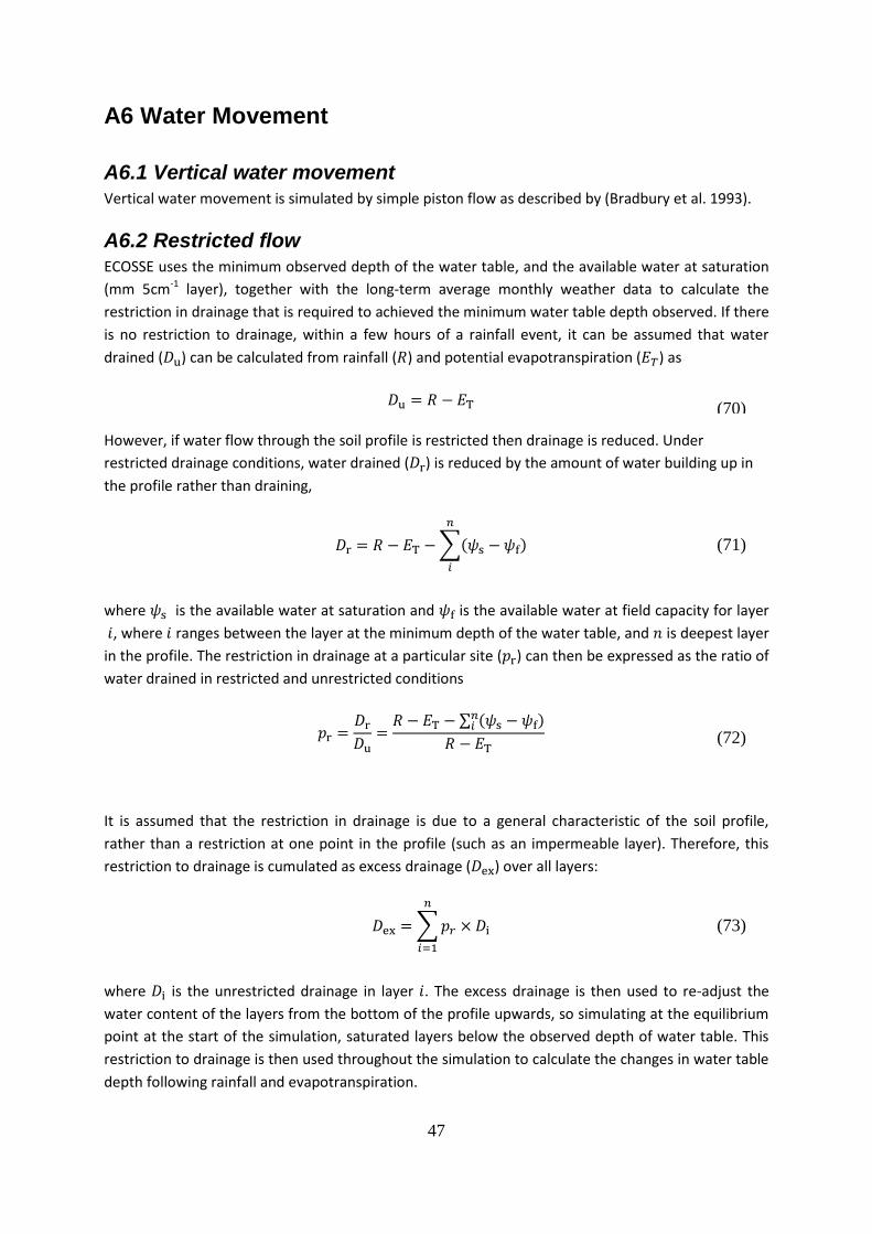
47

A6 Water Movement

A6.1 Vertical water movement

Vertical water movement is simulated by simple piston flow as described by (Bradbury et al. 1993).

A6.2 Restricted flow

ECOSSE uses the minimum observed depth of the water table, and the available water at saturation

(mm 5cm-1 layer), together with the long-term average monthly weather data to calculate the

restriction in drainage that is required to achieved the minimum water table depth observed. If there

is no restriction to drainage, within a few hours of a rainfall event, it can be assumed that water

drained ( ) can be calculated from rainfall ( ) and potential evapotranspiration ( ) as

However, if water flow through the soil profile is restricted then drainage is reduced. Under

restricted drainage conditions, water drained ( ) is reduced by the amount of water building up in

the profile rather than draining,

where is the available water at saturation and is the available water at field capacity for layer

, where ranges between the layer at the minimum depth of the water table, and is deepest layer

in the profile. The restriction in drainage at a particular site ( ) can then be expressed as the ratio of

water drained in restricted and unrestricted conditions

It is assumed that the restriction in drainage is due to a general characteristic of the soil profile,

rather than a restriction at one point in the profile (such as an impermeable layer). Therefore, this

restriction to drainage is cumulated as excess drainage ( ) over all layers:

where is the unrestricted drainage in layer . The excess drainage is then used to re-adjust the

water content of the layers from the bottom of the profile upwards, so simulating at the equilibrium

point at the start of the simulation, saturated layers below the observed depth of water table. This

restriction to drainage is then used throughout the simulation to calculate the changes in water table

depth following rainfall and evapotranspiration.

(73)

(72)

(71)

(70)

48

A6.3 Evaluation of ECOSSE simulations of water movement

An evaluation of the ECOSSE simulations of the water movement has been completed for a range of

soil conditions, in a number of different soil environments and under different land uses. This work is

currently being prepared for publication and so cannot be included here. When published, a


PART B - SITE SPECIFIC SIMULATIONS

B1 Input files

The formats of the input files for the site specific version are complex as they were originally

designed to be accessed via a DOS based graphical user interface, and not directly by the user.

However, with the development of the Windows operating system, the DOS interface is now

obsolete, and so users more often access the files directly using an editor. If you would like a copy of

the DOS-based graphical user interface, please contact the authors.

B1.1 Management Data

B1.1.1 Input through file MANAGEMENT.DAT

If file MANAGEMENT.DAT exists, this file will provide management data.

Format of example file is shown below. Data value is entered in the first 10 spaces of each line. The

2 Soil code number

2 Drainage class (1=low; 2=moderate; 3=high)

1 Depth to impermeable layer (1=50cm; 2=100cm; 3=150cm)

1 Previous crop (code given in CROP_SUN.DAT)

7 Yield of previous crop (t / ha)

35 Atmospheric N deposition (kg N / ha)

1 Date field reaches field capacity (1=01/01; 2=01/06)

1 Timestep (0 = 30 minute; 1 = daily; 2 = weekly; 3 = monthly)

0 Crop model type (0=SUNDIAL; 1=MAGEC)

10 Number of years included in the simulation

243 Timesteps from 01/01/01 to harvest of previous crop

2003 First year of simulation

3650 End of simulation

0 Fixed end of simulation (0=No; 1=Yes)

53 Latitude

' daily.dy ' Met.file year 1










9 Number of crops

6 CROP 1: Crop code (code given in CROP_SUN.DAT)

273 Timesteps to sowing date from 01/01/01

0 Crop N uptake at harvest (0 = calculate internally) kg N / ha

623 Timesteps to harvest date from 01/01/01

5 Expected yield (t/ha)

0 Crop residues incorporated (0=No; 1=Yes)

1 Number of fertiliser application

0 Number of manure applications

200 CROP 1, FERT 1: Amount of fertiliser applied (kg N / ha)

455 Timesteps to application date from 01/01/01

100 % Nitrate

0 % Non-urea N

0 % Urea N

0 Does fertiliser contain ammonium salts other than ammonium sulphate? (0=No; 1=Yes)

0 Is fertiliser labelled?

49

explanatory note on each line is not read by the model.

B1.1.2 Input by setup file

If MANAGEMENT.DAT does not exist, management is read in from SETUP file. The name of the SETUP

file is read in from FNAMES.DAT. Name of file is held within speech marks. The format of

FNAMES.DAT shown below.

The

format of the SETUP file is as given below. The top cells on each line shows the values entered in the

file in free format, space separated. The text in the lower cells indicates the meaning of each item.

Additional crops are added by repeating the lines shown for crop 1. Empty cells are omitted from the

file.

Line 1: 'sbarley.set'

Input variableSoil Type

(SOIL_PARS.DAT)Drainage class

Depth to

impermeable layer

Previous crop code

(PARLIS.OUT)

Previous crop

yield (t/ha)

Period under grass

in the past 10

years (not

changed)

Atmospheric N

deposition (kg

N / ha)

Date field reaches

field capacity

(1=01/01; 2=01/06)

12 2 2 6 5.53 1 0 1

"Waite" Moderate 100cm Spring Barley None Error! Too low! 1-Jan

Input variableNumber of years

included in the simulationDate of first harvest

First year in

simulation

Start of simulation (not

changed)

End of

simulation (not

changed)

Fixed end to

simulation? (0=No,

1=Yes)

Latitude

5 232 1988 1 1830 0 50

22-Aug-88 Error! Too high! No

Input variable Weather File

Line 3 ' eisen88.dy '

Line 4 ' eisen89.dy '

Line 5 ' '

Line 6 ' '

Line 7 ' '

Line 8 ' '

Line 9 ' '

Line 10 ' '

Line 11 ' '

Line 12 ' '

Input variable Number of crops

1

CROP 1

Input variable Crop code

(PARLIS.OUT)

Sowing date

Crop N uptake at

harvest (0 =

calculate internally)

Harvest dateExpected yield

(t/ha)

Crop residues

incorporated

(0=No, 1=Yes)

Number of

fertiliser

applications

Number of organic

manure

applications

Line 14 9 457 0 665 43.91 0 4 0

Maincrop Potatoes 5-Apr-1989 Calculate internally 30-Oct-1989 No

CROP 1

FERTILISERS

Input variable

Amount of fertiliser N

applied (kg N / ha)

Timesteps to

application date from

01/01/01

% Nitrate N % Non-Urea N % Urea N

Does fertiliser

contain ammonium

salts other than

ammonium

sulphate? (0=No;

1=Yes)

Is fertiliser

labelled?

(0=No; 1=Yes)

36 453 0 100 0 1 0

1-Apr-1989 Yes No

63 477 0 100 0 0 0

25-Apr-1989 No No

14 498 25 25 50 1 0

16-May-1989 Yes No

46 501 0 0 100 1 0

19-May-1989 Yes No

CROP 1

MANURES

Input variable

Amount of organic

manure applied (t

manure fresh weight /

ha)

Timesteps to

application date from

01/01/01

Manure typeIs manure labelled?

(0=No; 1=Yes)

Line 1

Line 2

Line 15

Line 13

Line 16

Line 17

Line 18

Line 19

Line 20

Line 21

Line 22

Line 23

Line 24

50

This example file is shown as it appears below.

B1.2. Weather Data Weather data is entered in files specified in management files. Note column titles are not included in

the input files. Data is entered as space separated values.

This example file is shown as it appears below.

B1.3 Crop Parameters

Crop parameters are entered through file CROP_SUN.DAT. The format of the file is as shown below:

Line 1: Crop name

Line 2: Crop code number

Timestep

number

Rainfall (mm

timestep-1)

Potential

Evapotranspiration

over Grass

(mm timestep-1)

Average air

temperature

(°C)

Daily global

radiation

(J m-2 ground d-1)

Daily minimum

temperature (°C)

Daily maximum

temperature (°C)

Vapour

pressure

(kPa)

Daily wind

speed (m s-1)

Line 1 1 10.9 0.2 1.9 2400000 -1.3 5.1 0.55 1.96

Line 2 2 5.5 -0.6 3.05 2000000 -0.8 6.9 0.87 3.08

… 3 0 0.2 2 3000000 0.9 3.1 0.5 2.8

…. 364 5.5 -0.2 9.25 600000 8 10.5 1.17 6.76

Line 365 365 9.3 0.5 7.95 1600000 6.4 9.5 0.91 3.43

MAGEC Crop Model OnlySUNDIAL Crop Model

12 2 2 6 5.53 1 0 1 1 0

5 232 1988 1 1830 0 50

'eisen88.dy' 0

'eisen89.dy' 0

1

9 457 0 665 43.91 0 4 0

36 453 0 100 0 1 0

63 477 0 100 0 0 0

14 498 25 25 50 1 0

46 501 0 0 100 1 0

1 10.9 0.2 1.9 2400000 -1.3 5.1 0.55 1.96

2 5.5 -0.6 3.05 2000000 -0.8 6.9 0.87 3.08

3 0 0.2 2 3000000 0.9 3.1 0.5 2.8

4 6.1 0.2 -0.1 2500000 -4.6 4.4 0.41 1.85

5 0.2 -0.5 -0.85 1000000 -3.8 2.1 0.66 3.34

6 0 0 0.55 2400000 -0.4 1.5 0.59 1.84

7 15.3 0.3 -1.4 1100000 -4 1.2 0.47 4.78

8 3.4 -0.1 0.2 900000 -0.6 1 0.62 1.67

9 4.2 0.6 3.8 2100000 0.1 7.5 0.64 2.5

10 2.3 -0.6 5.8 1300000 0.2 11.4 1.01 4.21

11 0 0.4 5.2 3300000 2.6 7.8 0.71 5.69

12 0 1.2 6.1 3500000 2.9 9.3 0.59 5.2

13 0 0.2 7.15 800000 3.3 11 0.95 7.35

14 0.2 0 6.15 3100000 5.3 7 0.88 7.5

15 0.3 0.5 4.65 1900000 3.6 5.7 0.69 3.74

16 0 0 1.35 3900000 -0.3 3 0.51 1.15

17 2.2 0.8 3.45 2800000 -2.6 9.5 0.57 2.4

18 0.5 -1.1 5.2 2100000 -0.3 10.7 1.13 4.79

19 4.2 0.4 9.9 1100000 9.2 10.6 1.1 5.93

20 3.1 0.6 4.4 3900000 0.9 7.9 0.63 5.12

21 0 -0.3 5.3 3600000 2.2 8.4 0.89 3.48

22 5.5 0.5 4.9 800000 0.6 9.2 0.73 5.08

51

Line 3: Parameters describing total C in crop debris: , , , and , as defined

in section A 5.7.1.

Line 4: Parameters describing uptake of N in below ground parts of the plant, , , ; and

parameters describing uptake of N in above ground parts of the plant, , , , as defined in

section A 5.7.3.

Line 5: Parameters describing the proportions of N in above and below ground crop that are

incorporated in the soil, and respectively as described in section A 5.7.3. Rate constants

for incorporation of C and N in debris before harvest, as described in section A 5.7.4.

Line 6: Fraction of N taken up by the crop that is senesced after anthesis, amount of N in seed (kg N

ha-1), Empirical parameters describing uptake of N by the crop, and , respectively, as described

in section A 5.7.5.

Line 7: Period of senescence (weeks); rate of root growth (cm week-1); depth above current root

depth from which N extraction can occur (cm); maximum rooting depth (cm).

Line 8: Empirical parameters describing C in the stubble (non-cartable crop debris), , , ,

and as described in section A 5.7.4.

Line 9: Parameters describing C and N in straw as described in section A 5.7.4; the harvest

index, the dry matter content of the straw (t dry matter / t straw), the C : dry matter

ratio of the straw, and the N : dry matter ratio of the straw (kg N / t straw dry matter).

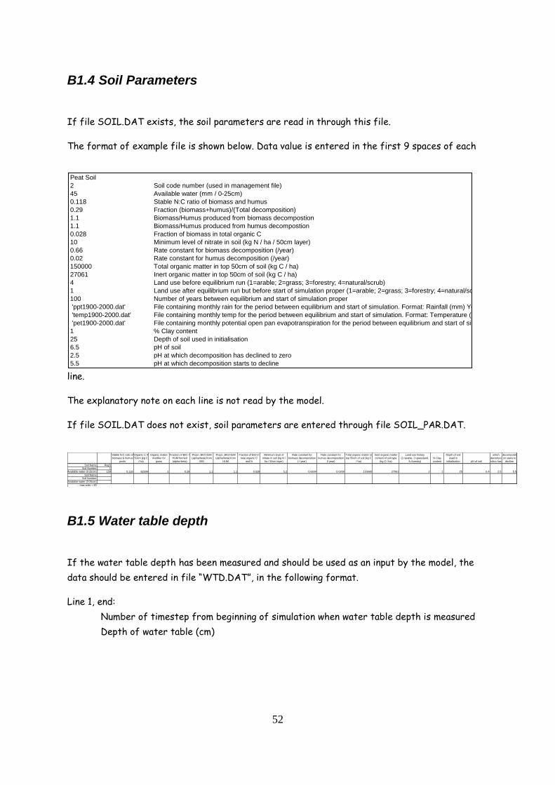
52

B1.4 Soil Parameters

If file SOIL.DAT exists, the soil parameters are read in through this file.

The format of example file is shown below. Data value is entered in the first 9 spaces of each

line.

The explanatory note on each line is not read by the model.

If file SOIL.DAT does not exist, soil parameters are entered through file SOIL_PAR.DAT.

B1.5 Water table depth

If the water table depth has been measured and should be used as an input by the model, the

data should be entered in file “WTD.DAT”, in the following format.

Line 1, end:

Number of timestep from beginning of simulation when water table depth is measured

Depth of water table (cm)

Stable N:C ratio of

biomass & humus

pools

Organic C 0-

50cm (kg C

/ ha)

Organic matter

modifier for

grass

Fraction of BIO +

HUM formed

(alpha+beta)

Propn. BIO:HUM

(alpha/beta) from

BIO

Propn. BIO:HUM

(alpha/beta) from

HUM

Fraction of BIO in

total organic C

and N

Minimum level of

nitrate in soil (kg N /

ha / 50cm layer)

Soil Name RegS

Soil Number 1

Available water (0-25cm) 159 0.118 82939 1 0.29 1.1 1.1 0.028 5.2

Soil Name

Soil Number

Available water (0-25cm)

… max soils = 20

Rate constant for

biomass decomposition

( / year)

Rate constant for

humus decomposition

(/ year)

Total organic matter in

top 50cm of soil (kg C

/ ha)

Inert organic matter

content of soil type

(kg C / ha)

Land use history

(1=arable, 2=grassland,

3=forestry)

% Clay

content

Depth of soil

used in

initialisation pH of soil

pH at

which

decompo

sition has

pH at which

decompositi

on starts to

decline

0.6604 0.0208 110000 27061 2 1 25 6.4 2.5 5.5

Peat Soil

2 Soil code number (used in management file)

45 Available water (mm / 0-25cm)

0.118 Stable N:C ratio of biomass and humus

0.29 Fraction (biomass+humus)/(Total decomposition)

1.1 Biomass/Humus produced from biomass decompostion

1.1 Biomass/Humus produced from humus decompostion

0.028 Fraction of biomass in total organic C

10 Minimum level of nitrate in soil (kg N / ha / 50cm layer)

0.66 Rate constant for biomass decomposition (/year)

0.02 Rate constant for humus decomposition (/year)

150000 Total organic matter in top 50cm of soil (kg C / ha)

27061 Inert organic matter in top 50cm of soil (kg C / ha)

4 Land use before equilibrium run (1=arable; 2=grass; 3=forestry; 4=natural/scrub)

1 Land use after equilibrium run but before start of simulation proper (1=arable; 2=grass; 3=forestry; 4=natural/scrub)

100 Number of years between equilibrium and start of simulation proper

'ppt1900-2000.dat' File containing monthly rain for the period between equilibrium and start of simulation. Format: Rainfall (mm) Year 1, month 1, 2, 3, 4, 5, 6, 7, 8, 9, 10, 11, 12; Year 2... (12(F8.0, 2X)/...)

'temp1900-2000.dat' File containing monthly temp for the period between equilibrium and start of simulation. Format: Temperature (deg.C) Year 1, month 1, 2, 3, 4, 5, 6, 7, 8, 9, 10, 11, 12; Year 2... (12(F8.0, 2X)/...)

'pet1900-2000.dat' File containing monthly potential open pan evapotranspiration for the period between equilibrium and start of simulation. Format: PET (mm) Year 1, month 1, 2, 3, 4, 5, 6, 7, 8, 9, 10, 11, 12; Year 2... (12(F8.0, 2X)/...)

1 % Clay content

25 Depth of soil used in initialisation

6.5 pH of soil

2.5 pH at which decomposition has declined to zero

5.5 pH at which decomposition starts to decline

53

B2 Output files

54

PART C - LIMITED DATA SITE SIMULATIONS

C1 Input files

C1.1 Site and management data New Line: Mode of equilibrium run: calculate C pools... 1=using known PI 2= adjusting PI to give measured TOC 3=adjusting decomp.rate to give meas.PI and TOC

4=using C accumulation 5=using fixed proportions of C pools 6=using TOC and the Hillier solver (analytical soln of RothC =brium run)

to get PI & C pools 7= adjusting PI to give measured TOC, and further adjusting PI during

dynamic phase of the simulation according to current weather

New Line: n = Number of layers (max. 10) New Line: Depth of top of SOM layer 1 (cm) New Line: Depth of top of SOM layer 2 (cm) New Line: ...Depth of top of SOM layer n (cm) For this soil under arable:

In SOM layer 1 New Line: C content (kg C / ha) New Line: Bulk density (g/cm

3)

New Line: Soil pH New Line: % clay by weight New Line: % silt by weight New Line: % sand weight

In SOM layer 2... In SOM layer n...

For this soil under grassland: In SOM layer 1

New Line: C content (kg C / ha) New Line: Bulk density (g/cm

3)



For this soil under forestry: In SOM layer 1


3)



For this soil under natural/seminatural: In SOM layer 1


3)

New Line: Soil pH New Line: % clay by weight

55

New Line: % silt by weight New Line: % sand weight


New Line: Arable long term average plant C input (kg C /ha/yr) (used in modes 1 & 3 only) New Line: Grassland long term average plant C input (kg C /ha/yr) (used in modes 1 & 3 only) New Line: Forestry long term average plant C input (kg C /ha/yr) (used in modes 1 & 3 only) New Line: Natural long term average plant C input (kg C /ha/yr) (used in modes 1 & 3 only) Long term average rainfall (mm/month) New Line: January New Line: February New Line: March New Line: April New Line: May New Line: June New Line: July New Line: August New Line: September New Line: October New Line: November New Line: December Long term average temperature (deg.C/month) New Line: January New Line: February New Line: March New Line: April New Line: May New Line: June New Line: July New Line: August New Line: September New Line: October New Line: November New Line: December New Line: Latitude New Line: Water table depth at start (cm) New Line: Drainage class (Not yet used) New Line: C accum.before change (kgC/ha/yr) (only in mode 4 – if not dummy value) New Line: CH4 emission before change (kgC/ha/yr) (not used yet) New Line: CO2 emission before change (kgC/ha/yr) (not used yet) New Line: DOC loss before change (kgC/ha/yr) (not used yet) New Line: Number of growing seasons, g New Line x g: For each growing season: Land use, plant input (kg C / ha / yr) – (not used in mode 7 - if plant input not given, unused and plant input obtained from RothC instead) 1=arable

2=grassland 3=forestry 4=natural/seminatural

New Line x g: Name of annual weather file (if used). If not given use long term average. (Format: Month,Rain(mm/mon),PET(mm/mon),Temp(deg.C/mon)) Note: need quotes round file name

Example file: 2 Mode of run 3 Number of layers 18 Depth of bottom of SOM layer 1 (cm) 68 Depth of bottom of SOM layer 2 (cm) 80 Depth of bottom of SOM layer 3 (cm) 196946 C content (kg C / ha) - for this soil under arable in SOM layer 1

56

0.34 Bulk density (g/cm3) - for this soil under arable in SOM layer 1 5.95 pH - for this soil under arable in SOM layer 1 7 % clay by weight - for this soil under arable in SOM layer 1 23 % silt by weight - for this soil under arable in SOM layer 1 70 % sand by weight - for this soil under arable in SOM layer 1 16462 C content (kg C / ha) - for this soil under arable in SOM layer 2 1.49 Bulk density (g/cm3) - for this soil under arable in SOM layer 2 5.91 pH - for this soil under arable in SOM layer 2 9 % clay by weight - for this soil under arable in SOM layer 2 21 % silt by weight - for this soil under arable in SOM layer 2 70 % sand by weight - for this soil under arable in SOM layer 2 7280 C content (kg C / ha) - for this soil under arable in SOM layer 3 1.52 Bulk density (g/cm3) - for this soil under arable in SOM layer 3 5.42 pH - for this soil under arable in SOM layer 3 12 % clay by weight - for this soil under arable in SOM layer 3 18 % silt by weight - for this soil under arable in SOM layer 3 70 % sand by weight - for this soil under arable in SOM layer 3 3 pH - for this soil under grassland in SOM layer 1 33 % clay by weight - for this soil under grassland in SOM layer 1 33 % silt by weight - for this soil under grassland in SOM layer 1 34 % sand by weight - for this soil under grassland in SOM layer 1 33 % silt by weight - for this soil under grassland in SOM layer 1 34 % sand by weight - for this soil under grassland in SOM layer 1 0 C content (kg C / ha) - for this soil under grassland in SOM layer 2 1.3 Bulk density (g/cm3) - for this soil under grassland in SOM layer 2 3 pH - for this soil under grassland in SOM layer 2 33 % clay by weight - for this soil under grassland in SOM layer 2 33 % silt by weight - for this soil under grassland in SOM layer 2 34 % sand by weight - for this soil under grassland in SOM layer 2 0 C content (kg C / ha) - for this soil under grassland in SOM layer 3 1.3 Bulk density (g/cm3) - for this soil under grassland in SOM layer 3 3 pH - for this soil under grassland in SOM layer 3 33 % clay by weight - for this soil under grassland in SOM layer 3 33 % silt by weight - for this soil under grassland in SOM layer 3 34 % sand by weight - for this soil under grassland in SOM layer 3 45100 C content (kg C / ha) - for this soil under forestry SOM layer 1 1.3 Bulk density (g/cm3) - for this soil under forestry in SOM layer 1 3 pH - for this soil under forestry in SOM layer 1 33 % clay by weight - for this soil under forestry in SOM layer 1 33 % silt by weight - for this soil under forestry in SOM layer 1 34 % sand by weight - for this soil under forestry in SOM layer 1 0 C content (kg C / ha) - for this soil under forestry SOM layer 2 1.3 Bulk density (g/cm3) - for this soil under forestry in SOM layer 2 3 pH - for this soil under forestry in SOM layer 2 33 % clay by weight - for this soil under forestry in SOM layer 2 33 % silt by weight - for this soil under forestry in SOM layer 2 34 % sand by weight - for this soil under forestry in SOM layer 2 0 C content (kg C / ha) - for this soil under forestry SOM layer 3 1.3 Bulk density (g/cm3) - for this soil under forestry in SOM layer 3 3 pH - for this soil under forestry in SOM layer 3 33 % clay by weight - for this soil under forestry in SOM layer 3 33 % silt by weight - for this soil under forestry in SOM layer 3 34 % sand by weight - for this soil under forestry in SOM layer 3 196946 C content (kg C / ha) - for this soil under semi-natural / natural in SOM layer 1 0.34 Bulk density (g/cm3) - for this soil under semi-natural / natural in SOM layer 1 3.34 pH - for this soil under semi-natural / natural in SOM layer 1 0 % clay by weight - for this soil under semi-natural / natural in SOM layer 1 0 % silt by weight - for this soil under semi-natural / natural in SOM layer 1 0 % sand by weight - for this soil under semi-natural / natural in SOM layer 1 458584 C content (kg C / ha) - for this soil under semi-natural / natural in SOM layer 2

57

0.21 Bulk density (g/cm3) - for this soil under semi-natural / natural in SOM layer 2 4.18 pH - for this soil under semi-natural / natural in SOM layer 2 0 % clay by weight - for this soil under semi-natural / natural in SOM layer 2 0 % silt by weight - for this soil under semi-natural / natural in SOM layer 2 0 % sand by weight - for this soil under semi-natural / natural in SOM layer 2 61330 C content (kg C / ha) - for this soil under semi-natural / natural in SOM layer 3 1.33 Bulk density (g/cm3) - for this soil under semi-natural / natural in SOM layer 3 4.55 pH - for this soil under semi-natural / natural in SOM layer 3 2 % clay by weight - for this soil under semi-natural / natural in SOM layer 3 10 % silt by weight - for this soil under semi-natural / natural in SOM layer 3 88 % sand by weight - for this soil under semi-natural / natural in SOM layer 3 3956 Arable plant C input (kg C /ha/year) only used if mode = 1 or 3 4665 Grassland plant C input (kg C /ha/year) 4665 Forestry plant C input (kg C /ha/year) 5000 Natural plant C input (kg C /ha/year) 177.97 Long term average Monthly Rainfall (mm) 126.78 162.32 88.9 83.05 83.54 85.22 105.49 149.88 178.6 202.18 200.38 1.26 Long term average monthlt temperature (deg.C) 1.16 2.84 4.89 7.89 10.65 11.96 11.86 9.7 7.18 3.32 2.16 58 Latitude 0 Water table depth at start (cm) 1 Drainage class 210 C accum.before change (kgC/ha/yr) – only used if mode = 4 232 CH4 emission before change (kgC/ha/yr) – only used if mode = 4 1880 CO2 emission before change (kgC/ha/yr) – only used if mode = 4 0 DOC loss before change (kgC/ha/yr)' – only used if mode = 4 26 Number of growing seasons 4 Land use 4 4 4 4 4 4 4 4 4 4 4 4

58

4 4 4 4 4 4 4 4 4 4 4 4 4 'NH200600_1980.dat' Weather files to be used in dynamic simulations 'NH200600_1981.dat' 'NH200600_1982.dat' 'NH200600_1983.dat' 'NH200600_1984.dat' 'NH200600_1985.dat' 'NH200600_1986.dat' 'NH200600_1987.dat' 'NH200600_1988.dat' 'NH200600_1989.dat' 'NH200600_1990.dat' 'NH200600_1991.dat' 'NH200600_1992.dat' 'NH200600_1993.dat' 'NH200600_1994.dat' 'NH200600_1995.dat' 'NH200600_1996.dat' 'NH200600_1997.dat' 'NH200600_1998.dat' 'NH200600_1999.dat' 'NH200600_2000.dat' 'NH200600_2001.dat' 'NH200600_2002.dat' 'NH200600_2003.dat' 'NH200600_2004.dat' 'NH200600_2005.dat'

C1.2 Weather data Note: no title line! Line 1-12: In free format with no commas: Month number (1-12), rainfall (mm/month), potential evapotranspiration (mm/month) and air temperature (

oC).

C2 Output files

59

PART D - SPATIAL SIMULATIONS

D1 Input files

The GIS simulations are driven through input files, that are supplied in the control file, GNAMES.DAT, which contains the names of all other files used in the simulation.

D1.1 File GNAMES.DAT Line 1: Name of input file containing NPP and soil information Line 2: Name of input file containing LU information For non-SSKIB run Line 3: Name of file containing soil codes Lines 4-6 = blank For SSKIB run = names of files containing Line 3: 1. soil codes under arable; Line 4: 2. soil codes under grassland; Line 5: 3. soil codes under forestry; Line 6: 4. soil codes under nat/semi-nat; Line 7: 5. soil codes under miscanthis; Line 8: 6. soil codes under SRC. Line 7: Name of output file for results on 1km

2 grid

Line 8: Name of output file for results on 20km2 grid

Line 9: Name of output file for results on 1km2 grid organic soil

Line 10: Name of output file for results on 20km2 grid organic soil

Line 11: Depth of reporting (cm) For Scottish data non-SSKIB and SSKIB climate change runs Line 12: Name of future climate file (if looking at climate change – if not just miss off) For JULES climate change run Line 12a: Name of future rainfall file (if looking at climate change – if not just miss off) Line 12b: Name of future temperature file (if looking at climate change – if not just miss off) Line 12c: Name of future NPP file (if looking at climate change – if not just miss off) For all climate change runs Line 13: Name of climate change results file (if looking at climate change – if not just miss off) Line 14: Name of climate change organic results file (if looking at climate change – if not just miss off)

D1.2 Input File for NPP and Soil Information Line 1: Title line Line 2 to end: Grid ID (20km

2)

Grid ID (1km2)

Eastings coordinate (m) Northings (m) Area of 1km

2 grid occupied by land (m

2)

Dominant soil series 1 Percentage of cell under dominant soil series 1 Soil wetness class series 1 Dominant soil series 2 Percentage of cell under dominant soil series 2 Soil wetness class series 2

60

Dominant soil series 3 Percentage of cell under dominant soil series 3 Soil wetness class series 3 Dominant soil series 4 Percentage of cell under dominant soil series 4 Soil wetness class series 4 Dominant soil series 5 Percentage of cell under dominant soil series 5 Soil wetness class series 5 Remaining percentage of cell under other soil series Net primary production kgC m

-2 x 1000 for this 1km

2 grid cell

Long Term Average Rainfall (mm month-1

) Jan to Dec

Long Term Average Air Temperature (C month-1

) Jan to Dec Longitude Lattitute

D1.3 Format of Input File for LU Information Line 1: Title line Line 2 to end: Grid ID (20km

2)

Grid ID (1km2)

Eastings coordinate (m) Northings (m) Area of 1km

2 grid occupied by land (m

2)

Fraction of cell under arable at start Fraction of cell under gardens at start (not used) Fraction of cell under semi-natural/natural at start Fraction of cell under other at start (not used) Fraction of cell under grassland at start Fraction of cell under sea at start (not used) Fraction of cell under forestry at start Fraction of cell under urban at start Fraction of cell under water at start Fraction of cell under land with non-CORINE definition at start Fraction of cell under miscanthus at start Fraction of cell under SRC at start LU1 changed to LU2 in decade 1 (ha decade

-1 20km

-2)

LU1=Forestry; LU2=Forestry; LU1=Natural/Semi-natural; LU2=Forestry; LU1=Grassland; LU2=Forestry; LU1=Arable; LU2=Forestry; LU1=Miscanthus; LU2=Forestry; LU1=SRC; LU2=Forestry; LU1=Forestry; LU2= Natural/Semi-natural; LU1=Natural/Semi-natural; LU2= Natural/Semi-natural; LU1=Grassland; LU2= Natural/Semi-natural; LU1=Arable; LU2= Natural/Semi-natural; LU1=Miscanthus; LU2= Natural/Semi-natural; LU1=SRC; LU2= Natural/Semi-natural;

LU1=Forestry; LU2=Grassland; LU1=Natural/Semi-natural; LU2=Grassland; LU1=Grassland; LU2=Grassland; LU1=Arable; LU2=Grassland; LU1=Miscanthus; LU2=Grassland; LU1=SRC; LU2=Grassland;

LU1=Forestry; LU2=Arable; LU1=Natural/Semi-natural; LU2=Arable; LU1=Grassland; LU2=Arable;

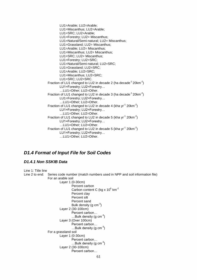
61

LU1=Arable; LU2=Arable; LU1=Miscanthus; LU2=Arable; LU1=SRC; LU2=Arable;

LU1=Forestry; LU2= Miscanthus; LU1=Natural/Semi-natural; LU2= Miscanthus; LU1=Grassland; LU2= Miscanthus; LU1=Arable; LU2= Miscanthus; LU1=Miscanthus; LU2= Miscanthus; LU1=SRC; LU2= Miscanthus;

LU1=Forestry; LU2=SRC; LU1=Natural/Semi-natural; LU2=SRC; LU1=Grassland; LU2=SRC; LU1=Arable; LU2=SRC; LU1=Miscanthus; LU2=SRC; LU1=SRC; LU2=SRC. Fraction of LU1 changed to LU2 in decade 2 (ha decade

-1 20km

-2)

LU1=Forestry; LU2=Forestry… …LU1=Other; LU2=Other. Fraction of LU1 changed to LU2 in decade 3 (ha decade

-1 20km

-2)

LU1=Forestry; LU2=Forestry… …LU1=Other; LU2=Other. Fraction of LU1 changed to LU2 in decade 4 (kha yr

-1 20km

-2)


-1 20km

-2)


-1 20km

-2)

LU1=Forestry; LU2=Forestry… …LU1=Other; LU2=Other.

D1.4 Format of Input File for Soil Codes

D1.4.1 Non SSKIB Data

Line 1: Title line Line 2 to end: Series code number (match numbers used in NPP and soil information file) For an arable soil

Layer 1 (0-30cm) Percent carbon Carbon content C (kg x 10

6 km

-2

Percent clay Percent silt Percent sand Bulk density (g cm

-3)

Layer 2 (30-100cm) Percent carbon…

…Bulk density (g cm-3

) Layer 3 (Over 100cm)

Percent carbon… …Bulk density (g cm

-3)

For a grassland soil Layer 1 (0-30cm)


-3)


62




-3)

For a semi-natural / natural soil Layer 1 (0-30cm)


-3)





-3)

For a forest soil Layer 1 (0-30cm)


-3)





-3)

For a miscanthus soil Layer 1 (0-30cm)


-3)





-3)

For a SRC soil Layer 1 (0-30cm)


-3)





-3)

D1.4.2 SSKIB Data

Note: -9999 = missing data. LU on this soil type is omitted from calculation. This provides a means of omitting unrealistic land uses (eg arable on peatland) Arable Soil Codes File Line 1: Title line Line 2 to end: Series code number (match numbers used in NPP and soil information file)

Flag for impermeable layer (0 = no impermeable/rock layer; 1 = impermeable / rock layer) Depth of impermeable layer (if present) (cm)

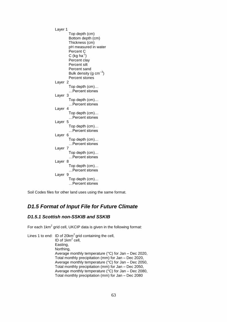
63

Layer 1 Top depth (cm) Bottom depth (cm) Thickness (cm) pH measured in water Percent C C (kg ha

-1)

Percent clay Percent silt Percent sand Bulk density (g cm

--3)

Percent stones Layer 2 Top depth (cm)… …Percent stones Layer 3 Top depth (cm)… …Percent stones Layer 4 Top depth (cm)… …Percent stones Layer 5 Top depth (cm)… …Percent stones Layer 6 Top depth (cm)… …Percent stones Layer 7 Top depth (cm)… …Percent stones Layer 8 Top depth (cm)… …Percent stones Layer 9 Top depth (cm)… …Percent stones Soil Codes files for other land uses using the same format.

D1.5 Format of Input File for Future Climate

D1.5.1 Scottish non-SSKIB and SSKIB

For each 1km2 grid cell, UKCIP data is given in the following format:

Lines 1 to end: ID of 20km

2 grid containing the cell,

ID of 1km2 cell,

Easting, Northing, Average monthly temperature (°C) for Jan – Dec 2020, Total monthly precipitation (mm) for Jan – Dec 2020, Average monthly temperature (°C) for Jan – Dec 2050, Total monthly precipitation (mm) for Jan – Dec 2050, Average monthly temperature (°C) for Jan – Dec 2080, Total monthly precipitation (mm) for Jan – Dec 2080

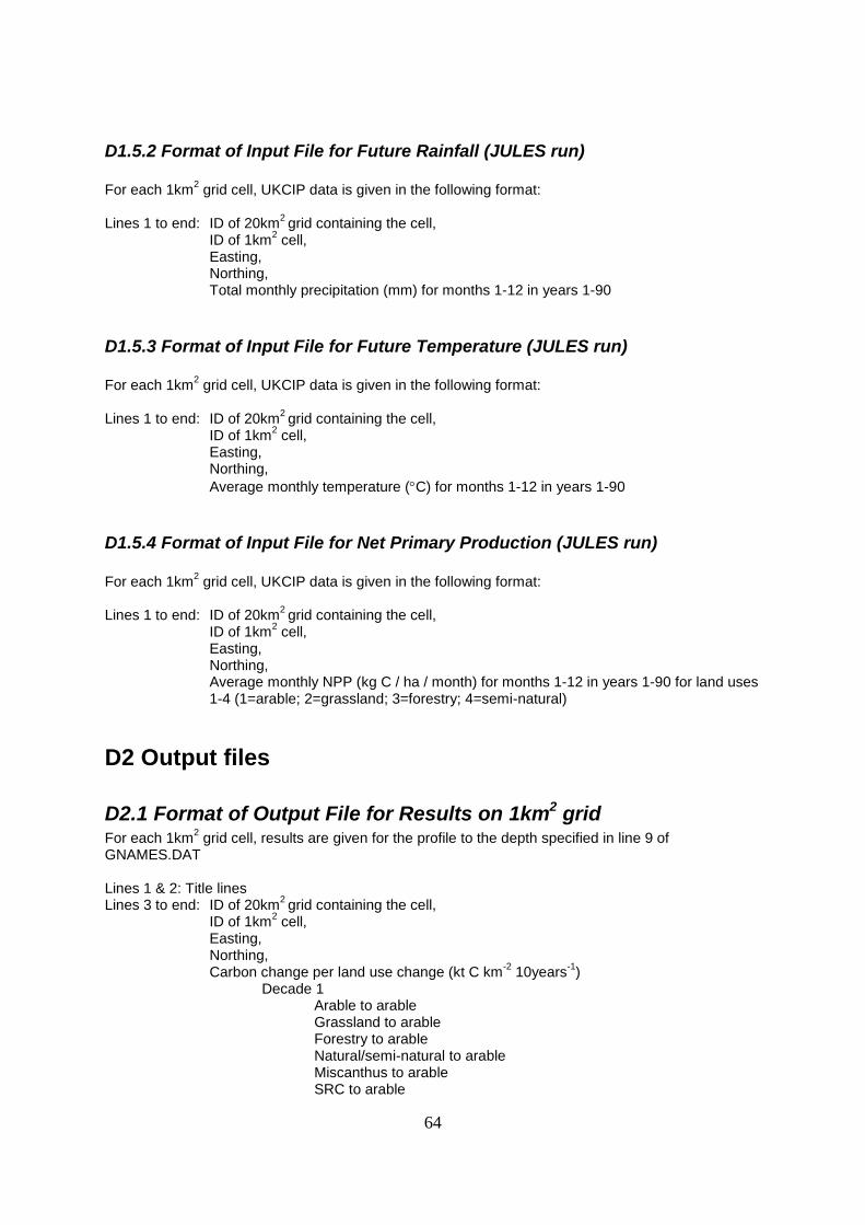
64

D1.5.2 Format of Input File for Future Rainfall (JULES run)




ID of 1km2 cell,

Easting, Northing, Total monthly precipitation (mm) for months 1-12 in years 1-90

D1.5.3 Format of Input File for Future Temperature (JULES run)




ID of 1km2 cell,

Easting, Northing,

Average monthly temperature (C) for months 1-12 in years 1-90

D1.5.4 Format of Input File for Net Primary Production (JULES run)




ID of 1km2 cell,

Easting, Northing, Average monthly NPP (kg C / ha / month) for months 1-12 in years 1-90 for land uses 1-4 (1=arable; 2=grassland; 3=forestry; 4=semi-natural)

D2 Output files

D2.1 Format of Output File for Results on 1km2 grid For each 1km

2 grid cell, results are given for the profile to the depth specified in line 9 of

GNAMES.DAT Lines 1 & 2: Title lines Lines 3 to end: ID of 20km


ID of 1km2 cell,

Easting, Northing, Carbon change per land use change (kt C km

-2 10years

-1)

Decade 1 Arable to arable Grassland to arable Forestry to arable Natural/semi-natural to arable Miscanthus to arable SRC to arable

65

Arable to grassland Grassland to grassland Forestry to grassland Natural/semi-natural to grassland Miscanthus to grassland SRC to grassland Arable to forestry Grassland to forestry Forestry to forestry Natural/semi-natural to forestry Miscanthus to forestry SRC to forestry Arable to natural/semi-natural Grassland to natural/semi-natural Forestry to natural/semi-natural Natural/semi-natural to natural/semi-natural Miscanthus to natural/semi-natural SRC to natural/semi-natural Arable to miscanthus Grassland to miscanthus Forestry to miscanthus Natural/semi-natural to miscanthus Miscanthus to miscanthus SRC to miscanthus Arable to SRC Grassland to SRC Forestry to SRC Natural/semi-natural to SRC Miscanthus to SRC SRC to SRC

Decade 2 Arable to arable ….

Decade 3

Arable to arable ….

Decade 4


Decade 5


Decade 6


Decade 7 (LU change projections using decade 6)


Carbon change for all soils in the cell (kt C km-2

10years-1

)

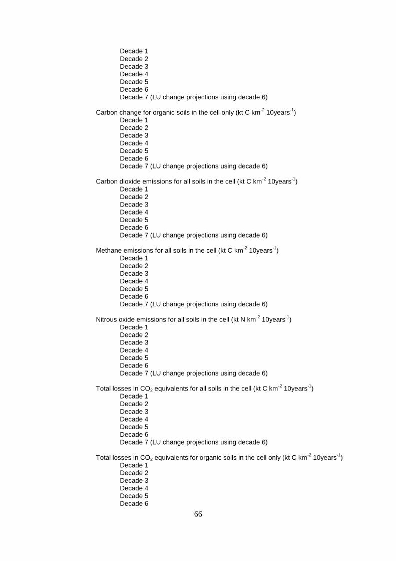
66

Decade 1 Decade 2 Decade 3 Decade 4 Decade 5 Decade 6 Decade 7 (LU change projections using decade 6)

Carbon change for organic soils in the cell only (kt C km

-2 10years

-1)


Carbon dioxide emissions for all soils in the cell (kt C km-2

10years-1

) Decade 1 Decade 2 Decade 3 Decade 4 Decade 5 Decade 6 Decade 7 (LU change projections using decade 6)

Methane emissions for all soils in the cell (kt C km

-2 10years

-1)


Nitrous oxide emissions for all soils in the cell (kt N km

-2 10years

-1)


Total losses in CO2 equivalents for all soils in the cell (kt C km-2

10years-1


Total losses in CO2 equivalents for organic soils in the cell only (kt C km

-2 10years

-1)

Decade 1 Decade 2 Decade 3 Decade 4 Decade 5 Decade 6

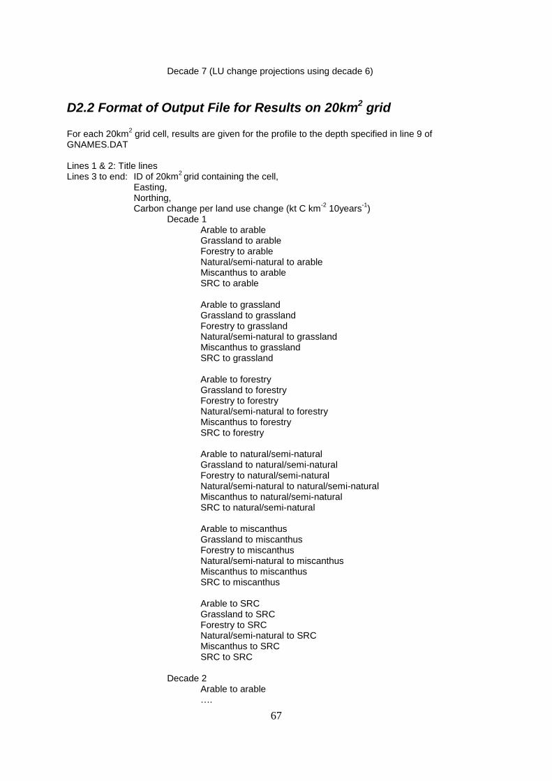
67

Decade 7 (LU change projections using decade 6)

D2.2 Format of Output File for Results on 20km2 grid

For each 20km2 grid cell, results are given for the profile to the depth specified in line 9 of

GNAMES.DAT Lines 1 & 2: Title lines Lines 3 to end: ID of 20km


Easting, Northing, Carbon change per land use change (kt C km

-2 10years

-1)

Decade 1 Arable to arable Grassland to arable Forestry to arable Natural/semi-natural to arable Miscanthus to arable SRC to arable Arable to grassland Grassland to grassland Forestry to grassland Natural/semi-natural to grassland Miscanthus to grassland SRC to grassland Arable to forestry Grassland to forestry Forestry to forestry Natural/semi-natural to forestry Miscanthus to forestry SRC to forestry Arable to natural/semi-natural Grassland to natural/semi-natural Forestry to natural/semi-natural Natural/semi-natural to natural/semi-natural Miscanthus to natural/semi-natural SRC to natural/semi-natural Arable to miscanthus Grassland to miscanthus Forestry to miscanthus Natural/semi-natural to miscanthus Miscanthus to miscanthus SRC to miscanthus Arable to SRC Grassland to SRC Forestry to SRC Natural/semi-natural to SRC Miscanthus to SRC SRC to SRC

Decade 2


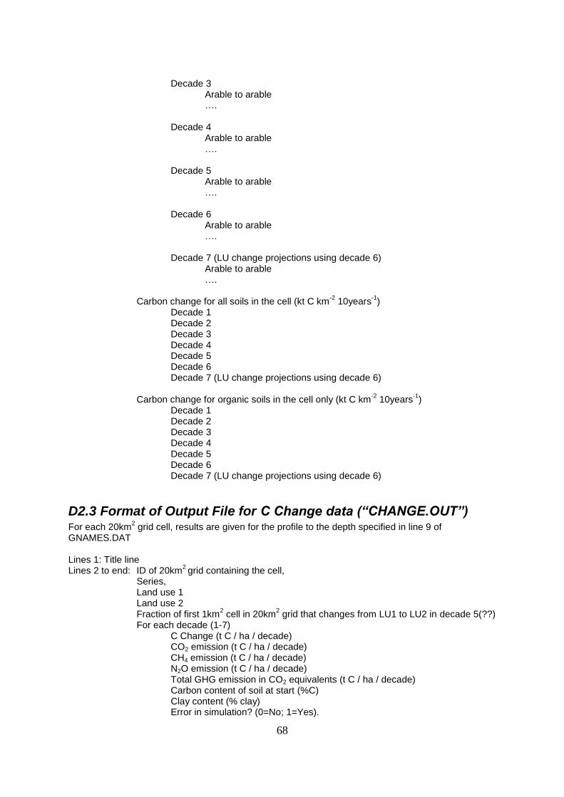
68

Decade 3


Decade 4


Decade 5


Decade 6


Decade 7 (LU change projections using decade 6) Arable to arable ….

Carbon change for all soils in the cell (kt C km-2

10years-1


Carbon change for organic soils in the cell only (kt C km

-2 10years

-1)


D2.3 Format of Output File for C Change data (“CHANGE.OUT”) For each 20km


GNAMES.DAT Lines 1: Title line Lines 2 to end: ID of 20km


Series, Land use 1 Land use 2 Fraction of first 1km

2 cell in 20km

2 grid that changes from LU1 to LU2 in decade 5(??)

For each decade (1-7) C Change (t C / ha / decade) CO2 emission (t C / ha / decade) CH4 emission (t C / ha / decade) N2O emission (t C / ha / decade) Total GHG emission in CO2 equivalents (t C / ha / decade) Carbon content of soil at start (%C) Clay content (% clay) Error in simulation? (0=No; 1=Yes).

69

D2.4 Format of Climate Change Results file For each 1km


GNAMES.DAT Line 1: Title line Lines 2 to end: ID of 20km


Easting, Northing, Carbon change per land use (t C km

-2 10years

-1)

Decade 1 Arable Grassland Forestry Natural/semi-natural Miscanthus SRC

Decade 2-7

Arable…

D2.5 Format of File for Calculation of Effects of Different Mitigation Options (files named MIT_A2P.OUT etc) For each 1km


GNAMES.DAT Lines 1 and 2: Title lines Lines 3 to end: ID of 20km


Easting, Northing,

Dominant soil series 1-5… Wetness class % C in top soil layer % clay in top soil layer Fraction 1km

2 cell that has this land use (km

2/km

2)

Decade 1-7… Carbon change associated with LU change applied in first decade (t C / ha / km

2 / decade)

70

PART E - REFERENCES

Aguilar L, Thibodeaux LJ (2005a) Kinetics of peat soil dissolved organic carbon release from bed sediment to

water. Part 1. Laborarory simulation. Chemosphere 58: 1309-1318

Aguilar L, Thibodeaux LJ (2005b) Kinetics of peat soil dissolved organic carbon release from bed sediment to

water. Part 2. A chemodynamic process model. Chemosphere 60: 1190-1196

Andersson S, Nilsson SI (2001) Influence of pH and temperature on microbial activity, substrate availability of

soil-solution bacteria and leaching of dissolved organic carbon in a mor humus. Soil Biol Biochem 33:1181–

1191

Bader FG (1978) Analysis of double-substrate limited growth. Biotechnol Bioeng 20:183-202

Bergman I, Lundberg P, Nilsson M (1999) Microbial carbon mineralisation in an acid surface peat: effects of

environmental factors in laboratory incubations. Soil Biol Biochem 31:1867-1877

Binkley D, Richter D (1987) Nutrient cycles and H+ budgets of forest ecosystems. Adv Ecol Res 16:1–51

Blagodatsky SA, Richter O (1998) Microbial growth in soil and nitrogen turnover: a theoretical model

considering the activity state of microorganisms. Soil Biology and Biochemistry 30:1743-1755

Blagodatsky SA et al (1998) Microbial growth in soil and nitrogen turnover: model calibration with laboratory

data. Soil Biology and Biochemistry 30:1757-1764

Blodau C, Basiliko N, Moore TR (2004) Carbon turnover in peatland mesocosms exposed to different water

table levels. Biogeochemistry 67: 331-351

Blodau C, Moore TR (2003) Experimental response of peatland carbon dynamics to a water table fluctuation.

Aquatic Sciences 65: 47-62

Bradbury NJ, Whitmore AP, Hart PBS, Jenkinson DS (1993) Modelling the fate of nitrogen in crop and soil in

the years following application of 15

N-labelled fertilizer to winter wheat. J Agr Sci 121: 363-379

Bridgham SD, Richardson CJ (1992) Mechanisms controlling soil respiration (CO2 and CH4) in southern

peatlands. Soil Biol Biochem 24:1089-1099

Christensen TR, Jonasson S, Callaghan TV, Havstrom M (1995) Spatial variation in high-latitude methane flux

along a transect across Siberian and European tundra environments. Journal of Geophysical Research –

Atmospheres 100: 21035-21045

Christensen TR, Prentice IC, Kaplan J, Haxeltine A, Sitch S (1996) Methane flux from northern wetlands and

tundra. Tellus 48:652-661

Christensen TR, Friborg T, Sommerkorn M, Kaplan J, Illeris L, Soegaard H, Nordstroem C, Jonasson S (2000)

Trace gas exchange in a high-arctic valley 1. Variations in CO2 and CH4 flux between tundra vegetation types.

Global Biogeochemical Cycles 14: 701-713

Coleman K, Jenkinson DS (1996) RothC-26.3 - A model the turnover of carbon in soil. In: Powlson DS, Smith

P, Smith JU (ed) Evaluation of soil organic matter models using existing long-term datasets. NATO ASI Series

I, vol. 38. Springer, Berlin, pp 237–246

Daulat WE, Clymo R (1998) Effects of temperature and water table on the efflux of methane from peatland

surface cores. Atmospheric Environment 32: 3207-3218

Devevre OC, Horwarth WR (2000) Decomposition of rice straw and microbial carbon use efficiency under

different soil temperatures and moistures. Soil Biol Biochem 32: 1773-1785

71

Doran JW, Mielke LN, Stamatiadis S (1988) Microbial activity and N cycling as regulated by soil water-filled

pore space. Proceedings of the 11th ISTRO Conference, Edinburgh, UK: 4954. Conference Organizing

Committee, Edinburgh, UK.

Dunfield P, Knowles R, Dumont R, Moore TR (1993) Methane production and consumption in temperate and

sub-arctic peat soils – response to temperature and pH. Soil Biology and Biochemistry 25: 321-326

Evans CD, Monteith DT, Cooper DM (2005). Long-term increases in surface water dissolved organic carbon:

observations, possible causes and environmental impacts. Environ Pollut 137: 55–71

Falloon P, Smith P, Coleman K, Marshall S (1998) Estimating the size of the inert organic matter pool for use in

the Rothamsted carbon model. Soil Biol Biochem 30: 1207-1211

Flynn HC, Smith J, Smith KA, Wright J, Smith P, Massheder J (2005) Climate- and crop-responsive emission

factors significantly alter estimates of current and future nitrous oxide emissions from fertiliser use. Global

Change Biology 11: 1522–1536

Frolking SE, Mosier AR, Ojima DS, Li C, Parton WJ, Potter CS, Priesack E, Stenger R, Haberbosch C, Dorsch

P, Flessa H, Smith KA (1998) Comparison of N2O emissions from soil at three temperate agricultural sites:

simulation of year-round measurements by four models. Nutrient Cycling in Agroecosystems 52:77-105

Garcia JL, Patel BKC, Ollivier B (2000) Taxonomic, phylogenetic, and ecological diversity of methanogenic

Archae. Anaerobe 6:205-226

Gilmore JT (1984) The effects of soil properties on nitrification and denitrification inhibition. Soil science

society of America Journal 48:1262-1266

Gorham E (1991) Northern peatlands: role in the carbon cycle and probable responses to climatic warming. Ecol

Appl 1:182-195. doi: 10.2307/1941811

Grundmann GL, Rolston DE (1987) A water function approximation to degree of anaerobiosis associated with

denitrification. Soil Science 144: 437-441

Hall JM, Paterson E, Killham K (1998) The effect of elevated CO2 concentration and soil pH on the relationship

between plant growth and rhizosphere denitrification potential. Glob Change Biol 4: 209-216

Hargreaves KJ, Fowler D (1998) Quantifying the effects of water table and soil temperature on the emission of

methane from peat wetland at the field scale. Atmospheric Environment 32: 3275-3282

Hargreaves KJ, Milne R, Cannell MGR (2003) Carbon balance of afforested peatland in Scotland. Forestry

76:299-317

Henault C, Germon JC (2000) NEMIS, a predictive model of denitrification on the field scale. European Journal

of soil Science 51: 257-270

Hutsch BW, Webster CP, Powlson DS (1994) Methane oxidation in soil as affected by land use, soil pH and N

fertilization. Soil Biology and Biochemistry 26: 1613-1622

Huttunen JT, Nykanen H, Martikainen PJ, Nieminen M (2003) Fluxes of nitrous oxide and methane from

drained peatlands following forest clear-felling in southern Finland. Plant and Soil 255: 457-462

Inubushi K, Otake S, Furukawa Y, Shibasaki N, Ali M, Itang AM, Tsuruta H (2005) Factors influencing

methane emission from peat soils: comparison of tropical and temperate wetlands. Nutrient cycling in

Agroecosystems 71:93-99

Jenkinson DS (1977) Studies on decomposition of plant material in soil .5. Effects of plant cover and soil type

on loss of carbon from 14

C labelled ryegrass decomposing under field conditions. J Soil Sci 28:424-434

72

Jenkinson DS, Rayner JH (1977) The turnover of organic matter in some of the Rothamsted classical

experiments. Soil Sci 123: 298–305

Jenkinson DS, Hart PBS, Rayner JH, Parry LC (1987) Modelling the turnover of organic matter in long-term

experiments at Rothamsted. INTECOL Bulletin 15:1-8

Joosten H (2009) The IMCG Global Peatland Database. www.imcg.net/gpd/gpd.htm

Jorgensen RG, Richter GM (1992) Composition of carbon fractions and potential denitrification in drained peat

soils. Journal of Soil Science 43: 347-358

Kettunen A (2002) Connecting methane fluxes to vegetation cover and water table fluctuations at microsite

level: a modelling study. Helsinki University of Technology. pp.41

Krug EC, Frink CR (1983). Acid rain on acid soil: a new perspective. Science 221: 520–525

Le Mer J, Roger P (2001) Production, oxidation, emission and consumption of methane by soils: a review.

European J Soil Biol 37:25-50

Leffelaar PA, Wessel WW (1988) Denitrification in a homogeneous closed system: experiment and simulation.

Soil Science 146:335-349

Leith H (1972) Modelling the primary productivity of the world. Nature and Resources, UNESCO, VIII, 2:5-10.

Li CS (2000) Modeling trace gas emissions from agricultural systems. Nutrient Cycling in Agroecosystems

58:259-276

Lloyd D, Thomas KL, Benstead J, Davies KL, Lloyd SH, Arah JRM, Stephens KD (1998) Methanogenesis and

CO2 exchange in an ombrotrophic peat bog. Atmospheric Environment 32: 3229-3238

MacDonald JA, Fowler D, Hargreaves KJ, Skiba U, Leith ID, Murray MB (1998) Methane emission rates from

a northern wetland; response to temperature, water table and transport. Atmospheric Environment 32: 3219-

3227

MacDonald JA, Skiba U, Sheppard LJ, Hargreaves KJ, Smith KA, Fowler D (1996) Soil environmental

variables affecting the flux of methane from a range of forest, moorland and agricultural soils. Earth and

Environment Science 34: 113-132.

Malhi SS, McGill WB (1982) Nitrification in three Alberta soils: effect of temperature, moisture and substrate

concentration. Soil Biology and Biochemistry 14:393-399

Maljanen M, Martikainen PJ, Aaltonen H, Silvola J (2002) Short-term variation in fluxes of carbon dioxide,

nitrous oxide and methane in cultivated and forested organic boreal soils. Soil Biology & Biochemistry 34: 577-

584

Michalzik B, Tipping E, Mulder J, Gallardo Lancho JF, Matzner E, Bryant CL, Clarke N, Lofts S, Vicente

Esteban MA (2003). Modelling the production and transport of dissolved organic carbon in forest soils.

Biogeochemistry 66: 241-264

Moore TR, Dalva M (1993) The influence of temperature and water-table position on carbon-dioxide and

methane emissions from laboratory columns of peatland soils. Journal of Soil Science 44: 651–664

Mosier A, Schimel D, Valentine D, Bronson K, Parton W (1991) Methane and nitrous-oxide fluxes in native,

fertilized and cultivated grasslands. Nature 350: 330-332

Motavalli PP, Palm CA, Parton WJ, Elliott ET, Frey SD (1995) Soil pH and organic carbon dynamics in tropical

forest soils with different mineralogies: Evidence from laboratory and modelling simulation studies. Soil Biol

Biochem 27:1589-1599

73

Parton WJ et al (1996) Generalized model for N2 and N2O production from nitrification and denitrification.

Global Biogeochemical Cycles 10:401-412

Palmer SM, Hope D, Billett MF, Dawson JJC, Bryant CL (2001) Sources of organic and inorganic carbon in a

headwater stream: evidence from carbon isotope studies. Biogeochemistry 52: 321-338

Persson T, Wiren A (1989) Microbial activity in forest soils in relation to acid/base and carbon/nitrogen status.

In: Braekke FN, Bjor K, Halvorsen B (ed) Air Pollution as Stress Factor in Nordic Forests. Norwegian Institute

for Forest Research, Aas, pp 83-95

Rask H, Schoenau J, Anderson D (2002) Factors influencing methane flux from a boreal forest wetland in

Saskatchewan, Canada. Soil Biol & Biochem 34:435-443

Reth S, Riechstein M, Falge E (2005) The effect of soil water content, soil temperature, soil pH-value and the

root mass on soil CO2 efflux – A modified model. Plant Soil 268:21-33.

Sabey BR, Frederick LR, Bartholomew WV (1959) The formation of nitrate from ammonium in soils III.

Influence of temperature and initial population of nitrifying organisms on the maximum rate and delay period.

Proceedings of the soil science society of America 23:462-465

Sitaula BK, Bakken LR, Abrahamsen G (1995) N-fertilization and soil acidification effects on N2O and CO2

emission from temperate pine forest soil. Soil Biol Biochem 27:1401-1408

Smith JU, Bradbury NJ, Addiscott TM (1996) SUNDIAL: A PC-based system for simulating nitrogen dynamics

in arable land. Agron J 88:38-43

Stanford G, Epstein E (1974) Nitrogen mineralization-water relations in soils. Soil Sci Soc Am J 38: 103-107

Wang ZP, Lindau CW, Delaune RD, Patrick WH (1993) Methane emissions and entrapment in flooded rice

soils as affected by soil properties. Biology and Fertility of Soils 16: 163-168

Weier KL et al (1993) Denitrification and the dinitrogen/nitrous oxide ration as affected by soil water, available

carbon, and nitrate. Soil science society of America Journal 57:66-72

Wickland KP, Striegl RG, Mast MA, Clow DW (2001) Carbonn exchange at a southern Rocky Mountain

wetland, 1996-1998. Global Biogeochemical cycles 15:321-335

Wickland KP, Striegl RG, Schmidt SK, Mast MA (1999) Methane flux in subalpine wetland and unsaturated

soils in the southern Rocky Mountains. Global Biogeochemical Cycles 13:101-113

Williams RI, Crawford RL (1984) Methane production in Minnesota peatlands. Applied and Environmental

Microbiology 47: 1266-1271

Williams RI, Crawford RL (1985) Methanogenic bacteria, including an acid-tolerant strain, from peatlands.

Applied and Environmental Microbiology 50:1542-1544

Zhang Y, Li C, Zhou X, Moore B (2002) A simulation model linking crop growth and soil biogeochemistry for

sustainable agriculture. Ecol Mod 151: 75-108

model to estimate carbon in organic soils sequestration ... user man… · model to estimate carbon...

Documents