NBER WORKING PAPER SERIES

LOBBYING COMPETITION OVER TRADE POLICY

Kishore GawandePravin Krishna

Marcelo Olarreaga

Working Paper 11371http://www.nber.org/papers/w11371

NATIONAL BUREAU OF ECONOMIC RESEARCH1050 Massachusetts Avenue

Cambridge, MA 02138May 2005

© 2005 by Kishore Gawande, Pravin Krishna, and Marcelo Olarreaga. All rights reserved. Short sectionsof text, not to exceed two paragraphs, may be quoted without explicit permission provided that fullcredit, including © notice, is given to the source.

Lobbying Competition Over Trade PolicyKishore Gawande, Pravin Krishna, and Marcelo OlarreagaNBER Working Paper No. 11371May 2005, Revised May 2009JEL No. D72,D78,F12,F13

ABSTRACT

Competition between opposing lobbies is an important factor in the endogenous determination of tradepolicy. This paper investigates empirically the consequences of lobbying competition between upstreamand downstream producers for trade policy. The theoretical structure underlying the empirical analysisis the well-known Grossman-Helpman model of trade policy determination, modified suitably to accountfor the cross-sectoral use of inputs in production (itself a quantitatively significant phenomenon witharound 50 percent of manufacturing output being used by other sectors rather than in final consumption).Data from more than 40 countries are used in our analysis. Our empirical results validate the predictionsof the theoretical model with lobbying competition. Importantly, accounting for lobbying competitionalso alters substantially estimates of the“welfare-mindedness” of governments in setting trade policy.

Kishore GawandeBush School of GovernmentTexas A&M UniversityTexas A&M UniversityCollege Station, TX 77840-4220kgawande@tamu.edu

Pravin KrishnaJohns Hopkins University1740 Massachusetts Avenue, NWWashington, DC 20036and NBERPravin_Krishna@jhu.edu

Marcelo OlarreagaDepartment of Political EconomyUniversity of GenevaUni Mail, 102 Bd Carl-Vogt, CH-1211 Geneve 4Marcelo.Olarreaga@ecopo.unige.ch

I. Introduction

Interest-group theories of endogenous trade policy determination describe trade policy out-

comes as resulting from the interaction between governments and special-interest lobbies. As

lobbies representing different economic interests may each seek to move policy in a different

direction, theoretical predictions regarding policy outcomes remain sensitive to the nature

and extent of competition between lobbies. Consider, for instance, policy determination

in the textbook, partial-equilibrium model of the market for final-good importables. Since

trade barriers against imports raise profits of domestic suppliers, these suppliers have an

incentive to lobby the government for such barriers to be imposed in their respective sectors;

the more susceptible government policy is to special interest lobbying, the greater the pre-

dicted departures from free trade.1 Alternately, in a more general context, where producers

are linked across sectors by their use of each others’ outputs as intermediates in their own

production, the pattern of lobbying and equilibrium protection can be expected to be more

complex. In particular, manufacturers would have an incentive to lobby for lower tariffs on

goods they use as inputs − in direct opposition to suppliers of these inputs who would favor

high barriers instead.2 Since these competing lobbies may cancel each other out, free trade

may emerge as an equilibrium even in settings where governments are highly amenable to

lobbying. Thus, the degree of lobbying competition matters crucially and studying its scope

and extent is important for understanding the determinants of the policies we observe.

It is the goal of this paper to examine empirically the political economy of trade policy

determination in the presence of lobbying competition − where the competition over policy

is assumed to arise out of the opposing interests of upstream and downstream producers of

goods. The approach we take here is a structural one. As a theoretical platform for our

1While consumers are hurt by these barriers and may be expected to lobby against them as well, theanalysis usually makes the (empirically compelling) assumption that consumers are not well organized intopro-trade lobbies. See Olson (1965) for potential explanations.

2A recent example is the lobbying for the removal of protection on steel imports by automobile manu-facturers in the United States. As reported by the Wall Street Journal (on December 16, 2006), “The steelantidumping duties in the US were brought down partly by a coalition of otherwise rival firms. The caseagainst the steel duties brought together rival U.S. and Japanese auto makers – General Motors Corp., Ford,and Daimler-Chrysler AG joined forces with Toyota Motor Corp., Honda Motor Co., and Nissan Motor Co.”.

1

empirical analysis, we use the well-known interest-group model of endogenous trade policy

determination provided by Grossman and Helpman (1994) - henceforth GH - who model

governments as trading away economic welfare for political contributions by lobbies. In GH,

protection is thus sold to lobbies and the level of protection provided to any industry is

derived as a function of certain industry characteristics (such as the presence of lobbies, the

import-demand elasticity and the import-penetration ratio) and, importantly, the rate at

which the government trades off welfare for political contributions. Our empirical analysis

is based on a simple modification of this framework that takes into explicit account the

extent of cross-sectoral use of intermediates in production (the input-output matrix),3 itself

a quantitatively significant phenomenon with around 50 percent of a sector’s output being

used by other sectors rather than in final consumption.

In addition to our intrinsic interest in the extent and consequence of lobbying competition,

our study is motivated by a puzzle that has been identified in the empirical literature.

Many empirical examinations of interest-group theory of trade policy determination using

US data (Goldberg and Maggi (1999) and Gawande and Bandyopadhyay (2000)) have found

evidence supporting the idea that trade protection is indeed for sale. However, all of these

studies report very high estimates of the “welfare-mindedness” of governments (measured

as the inverse of the rate at which the government trades off aggregate welfare for lobbying

contributions). That is, the government appears to be close to welfare-maximizing in its

behavior − demanding very high political contributions in exchange for a small amount of

distortionary protection. This finding sits poorly with casual observations on the extent of

lobbying and regulatory capture that appears to be taking place in most countries around

the world and with specific findings in other studies (albeit not related to trade policy) that,

if anything, policy distortions are being sold very cheap. However, our earlier discussion

suggests that lobbying competition modifies the picture in important ways. Specifically,

imagine that competition between lobbies leads to free trade as an equilibrium outcome

3We should note that in GH, owners of capital in a given sector are able to lobby for lower protection onfinal goods that they consume. While this serves as a reasonable theoretical proxy for intermediates use inproduction, from an empirical standpoint this framework suffers from at least the deficiency that consumptionpreferences of producers are assumed identical across sectors while intermediates use in different industriesis clearly considerably heterogeneous in practice.

2

with a government that is willing to sell policy distortions cheap. Observing the free trade

outcome, but ignoring the extent of lobbying competition, may lead an analyst to conclude

− incorrectly − that policy is being set by a welfare-maximizing government. Accounting

for lobbying competition is thus important for the evaluation of the welfare-mindedness of

governments in setting trade policy.

Two previous examinations of the Grossman-Helpman model, Gawande and Bandopadhyay

(2000) and McCalman (2004), have featured intermediates inputs. The primary motivation

for including the use of intermediates in the Gawande-Bandyopodhyay and McCalman papers

is to study the links between final goods tariffs and the tariffs on intermediate goods used in

their production. In particular, these papers show that the higher the tariff on the output of

the intermediate good, the greater is the tariff on its user. This is essentially a demonstration

of the pass-through argument that has been well documented (outside the political-economy

context) in the literatures on tariff escalation and effective protection. Our motivation,

instead, is to advance a theory of lobbying competition by users of intermediates in order

to formally model the natural opposition to tariffs on intermediates (say, steel) by users

of those intermediates (say, automobiles). Furthermore, in contrast to these earlier papers

which feature a single intermediates goods sector, our theoretical structure allows for as

many intermediate-good producing sectors as required. This is important from an empirical

perspective: A brief look at the U.S. input-output tables clearly indicates that any single

manufacturing sector uses intermediates produces in a disparate and wide-ranging group of

other sectors (and from within its own sector) − as is to be expected given the extent of

complexity and specialization manifest in today’s manufacturing technology. Overall, our

framework is different from both these earlier papers in its motivation, its execution and

finally, as will become clear, in its predictions as well.

In our empirical implementation, we use data from more than 40 countries spanning a wide

per capita income range. This is in contrast with most of the recent empirical studies on the

endogenous determination of trade policy, which have focused on the United States. Our

use of data from a wider range of countries enables a more robust evaluation of the role of

3

lobbying competition. We study the determinants of trade policy considering each country

separately and exploit the cross sectional variation across industries within any country to

obtain estimates of the “welfare-mindedness” of governments. Our findings are as follows.

First, lobbying competition between upstream and downstream producers appears to be

a statistically and quantitatively significant determinant of trade policy. This is a robust

finding extending through nearly our entire sample of countries. Second, with lobbying

competition taken into account, our country-specific estimate of the “welfare-mindedness”

of governments is lowered significantly in virtually every country in our sample (just as we

have anticipated in our theoretical discussion in the preceding paragraph). These findings

attest to the importance of lobbying competition in the endogenous determination of trade

policy.

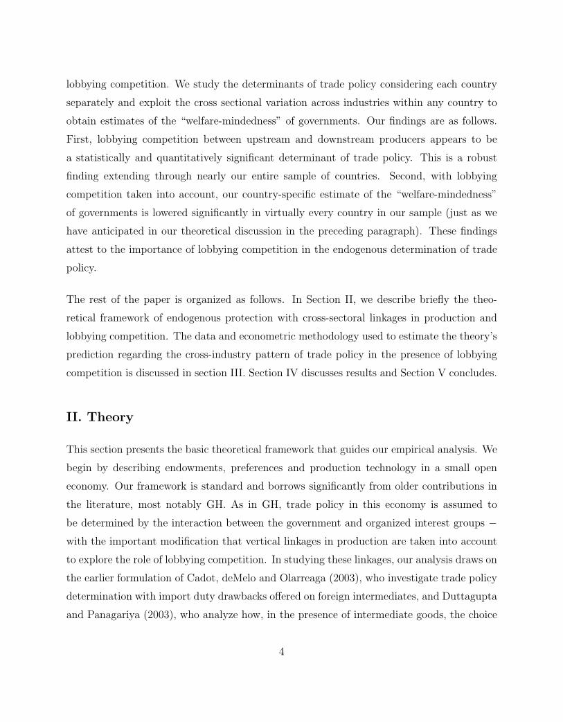
The rest of the paper is organized as follows. In Section II, we describe briefly the theo-

retical framework of endogenous protection with cross-sectoral linkages in production and

lobbying competition. The data and econometric methodology used to estimate the theory’s

prediction regarding the cross-industry pattern of trade policy in the presence of lobbying

competition is discussed in section III. Section IV discusses results and Section V concludes.

II. Theory

This section presents the basic theoretical framework that guides our empirical analysis. We

begin by describing endowments, preferences and production technology in a small open

economy. Our framework is standard and borrows significantly from older contributions in

the literature, most notably GH. As in GH, trade policy in this economy is assumed to

be determined by the interaction between the government and organized interest groups −with the important modification that vertical linkages in production are taken into account

to explore the role of lobbying competition. In studying these linkages, our analysis draws on

the earlier formulation of Cadot, deMelo and Olarreaga (2003), who investigate trade policy

determination with import duty drawbacks offered on foreign intermediates, and Duttagupta

and Panagariya (2003), who analyze how, in the presence of intermediate goods, the choice

4

of rules of origin alters the political feasibility of free trade agreements.4

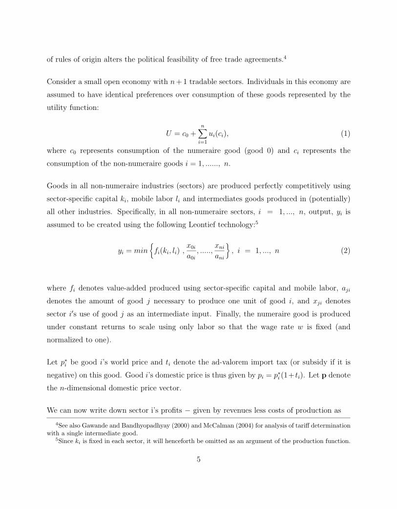
Consider a small open economy with n+1 tradable sectors. Individuals in this economy are

assumed to have identical preferences over consumption of these goods represented by the

utility function:

U = c0 +n∑

i=1

ui(ci), (1)

where c0 represents consumption of the numeraire good (good 0) and ci represents the

consumption of the non-numeraire goods i = 1, ......, n.

Goods in all non-numeraire industries (sectors) are produced perfectly competitively using

sector-specific capital ki, mobile labor li and intermediates goods produced in (potentially)

all other industries. Specifically, in all non-numeraire sectors, i = 1, ..., n, output, yi is

assumed to be created using the following Leontief technology:5

yi = min{fi(ki, li) ,

x0i

a0i

, .....,xni

ani

}, i = 1, ..., n (2)

where fi denotes value-added produced using sector-specific capital and mobile labor, aji

denotes the amount of good j necessary to produce one unit of good i, and xji denotes

sector i′s use of good j as an intermediate input. Finally, the numeraire good is produced

under constant returns to scale using only labor so that the wage rate w is fixed (and

normalized to one).

Let p∗i be good i’s world price and ti denote the ad-valorem import tax (or subsidy if it is

negative) on this good. Good i’s domestic price is thus given by pi = p∗i (1+ ti). Let p denote

the n-dimensional domestic price vector.

We can now write down sector i’s profits − given by revenues less costs of production as

4See also Gawande and Bandhyopadhyay (2000) and McCalman (2004) for analysis of tariff determinationwith a single intermediate good.

5Since ki is fixed in each sector, it will henceforth be omitted as an argument of the production function.

5

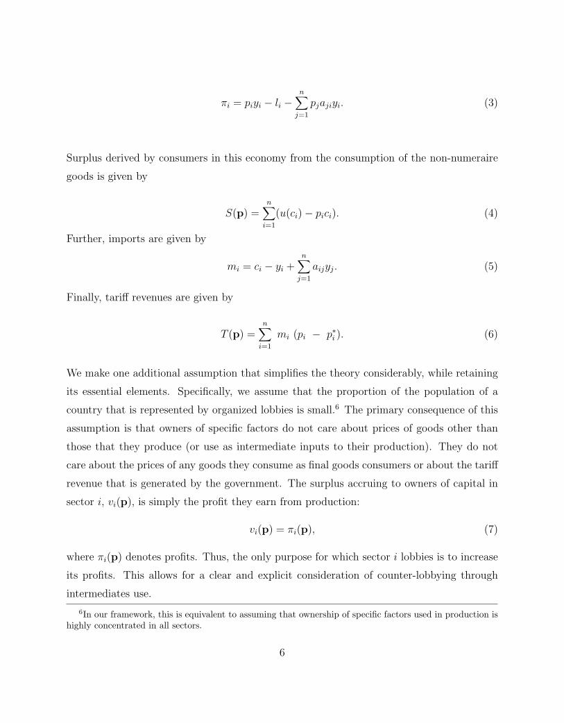
πi = piyi − li −n∑

j=1

pjajiyi. (3)

Surplus derived by consumers in this economy from the consumption of the non-numeraire

goods is given by

S(p) =n∑

i=1

(u(ci) − pici). (4)

Further, imports are given by

mi = ci − yi +n∑

j=1

aijyj. (5)

Finally, tariff revenues are given by

T (p) =n∑

i=1

mi (pi − p∗i ). (6)

We make one additional assumption that simplifies the theory considerably, while retaining

its essential elements. Specifically, we assume that the proportion of the population of a

country that is represented by organized lobbies is small.6 The primary consequence of this

assumption is that owners of specific factors do not care about prices of goods other than

those that they produce (or use as intermediate inputs to their production). They do not

care about the prices of any goods they consume as final goods consumers or about the tariff

revenue that is generated by the government. The surplus accruing to owners of capital in

sector i, vi(p), is simply the profit they earn from production:

vi(p) = πi(p), (7)

where πi(p) denotes profits. Thus, the only purpose for which sector i lobbies is to increase

its profits. This allows for a clear and explicit consideration of counter-lobbying through

intermediates use.

6In our framework, this is equivalent to assuming that ownership of specific factors used in production ishighly concentrated in all sectors.

6

Note that the free trade level of utility derived by owners of capital in the various sectors can

be obtained by evaluating (7) at pi = p∗i ∀i. Furthermore, trade interventions that move the

domestic price vector p away from free trade vector of prices may bring higher utility levels

to owners of capital in these sectors − giving rise to an incentive to lobby the government

to implement such interventions.

Lobbying and Endogenous Policy Determination

As in Grossman and Helpman (1994), the government is assumed to care about both the

political contributions that it receives from organized lobbies and about aggregate welfare;

contributions being valued because of their use in financing campaign spending or in the

direct benefits they provide to office holders and social welfare being of concern to the gov-

ernment due to the higher likelihood of voters re-electing a government that has delivered a

high standard of living. A linear objective function is assumed to represent these preferences:

G(p) =∑

i

Ci(p) + aW(p) (8)

where G(p) is the objective function of the government, Ci(p) is the contribution schedule

of the ith industry, W (p), is gross social welfare and a is the weight the government attaches

to social welfare relative to political contributions. Clearly, the higher is a, the higher its

concern for social welfare relative to its affinity for political contributions.

It is worth noting that in (8), we assume that all industries are politically organized. This

assumption is made here for several practical reasons. First, the level of industry aggregation

we will consider in the empirical section is the 3-digit ISIC level, implying 29 manufacturing

sectors. At this level of aggregation, industry associations and other forms of political

organization are pervasive across all industries and countries. For instance, in U.S. data,

significant contributions to the political process are reported by all 3-digit industries (and

indeed industries at much finer levels of dis-aggregation). Furthermore, the United States is

exceptional, even among the most developed nations, in the explicit reporting requirement of

political contributions by firms and industries. Since political contributions, while pervasive,

7

are simply not publicly disclosed in any of the other countries that we consider in our analysis,

this assumption relieves us of the burden of using ad hoc methods of determining the political

organization of industries (as have sometimes been used in studies involving US trade policy,

where such data on political contributions is indeed available as we have indicated).

Lobby welfare net of contributions is given by vi(p) − Ci(p). Efficiency of interaction be-

tween the government and organized lobbies dictates that the policy outcome is one which

maximizes their joint surplus:

G(p) +∑

i

(vi(p) − Ci(p)) =∑

i

πi(p) + aW(p) (9)

The tariffs that maximize the joint surplus must satisfy the following first order conditions:

n∑i

∂πi

∂pi

+ a∂W

∂pi

= 0 ∀i (10)

Using equations (1) through (10) above, and recognizing that ∂πi

∂pi= yi(1 − aii) ∀ i and

that ∂πi

∂pj= −ajiyi ∀ j 6= i, we have equilibrium ad valorem tariff protection in industry i,

ti = pi/p∗i − 1, with ti given by

ti1 + ti

=1

a

1

mi · |ei|

yi −n∑

j=1

aijyj

, (11)

where |εi| denotes the absolute value of the import-demand elasticity in sector i.

Equation (11) is the final theoretical prediction that emerges regarding trade protection

in the presence of lobbying competition. The interpretation of terms appearing in (11) is

straightforward. Lobbying competition between upstream and downstream users to raise

production profits is captured by the term in square brackets on right-hand side of the

equation. Lobbying by downstream users (∑n

j=1 aijyj 6= 0) lowers the level of protection

8

predicted. Equation (11) indicates that tariffs are lower the greater is a, the relative value

that the government places on aggregate welfare, and the greater is the import-demand

elasticity (for the usual Ramsey-pricing reasons).7

To summarize, we develop our cross-sectional prediction on trade protection (Equation (11))

using theoretical building blocks that are standard in the literature. Equation (11) allows

for estimation of the country specific parameter a, measuring the welfare-mindedness of

governments, taking into suitable account the extent of cross-sectoral lobbying competition

in the economy. The following sections discuss the data we use to conduct this estimation

analysis and also our empirical methodology and results.

III. Data

The econometric analysis that follows is based on the theoretically derived expression (11),

which describes the cross-sectional variation in trade policy with counter-lobbying. For this,

we use data from over 40 different countries (essentially all of the countries for which we

were able to gather the requisite data). The countries in our sample are Argentina, Aus-

tralia, Bangladesh, Chile, China, Cameroon, Colombia, Costa Rica, Denmark, Ecuador,

Finland, France, Germany, Greece, Guatemala, Hungary, Indonesia, Ireland, Italy, Japan,

Kenya, Mauritius, Mexico, Malaysia, Netherlands, Norway, Pakistan, Peru, Philippines, Ro-

mania, Singapore, South Africa, South Korea, Sri Lanka, Spain, Sweden, Thailand, Taiwan,

Uruguay, United Kingdom, United States and Venezuela.

7We should discuss, in closing, the robustness of our theoretical structure, in which final goods producersoppose increases in their input prices. As such, this effect clearly obtains in settings where producers lackmarket power. Even with imperfect competition, when firms’ strategies are strategic substitutes (as is thecase with quantity competition) or when firms hold consistent conjectures, the same result is easily obtained.However, when firms strategies are strategic complements (as would be the case with price competition), itis possible (when some further restrictions on demand are satisfied) to have outcomes in which an increasein input prices results in an increase in firm profits. While we do not consider this explicitly theoretically,our econometric exercises not impose any prior restrictions on this effect. We simply allow the data to guideus on this point.

9

For each of our sample countries, we have tariff data across twenty-eight 3-digit ISIC indus-

tries over the 1988-2000 period. The tariff data are the applied most-favored-nation (MFN)

rates from UNCTAD’s Trains database. The 6-digit Harmonized System level tariff data

available in TRAINS database were mapped into the 3-digit ISIC industries using filters

available from the World Bank site www.worldbank.org/trade. Where necessary and possi-

ble, those data are augmented by WTO applied rates, constructed from the WTO’s IDB and

WTO’s Trade Policy Reviews. The correlation between the two tariff series is greater than

0.93. Further, the direct and reverse regression coefficients are above 0.9, indicating that

the errors in variables problem from mixing the two data sources is not a concern. Across

our sample of countries and industries, tariff data are available for an average of 7.2 years

(minimum 2 and maximum 13). Data are nearly complete for the higher income countries

with lower-middle and low income countries sufficiently broadly covered to permit credible

inferences about the model parameters.

Industry level output and trade data are from the World Bank’s Trade and Production

database. Output data are taken from the UNIDO’s INDSTAT 3-digit ISIC rev. 2 database.

Import demand elasticities are estimated for each country at the 6-digit HS level using a

revenue function approach by Kee, Nicita and Olarreaga (2008). Since the standard errors

of the elasticity estimates are known, they are treated as variables with measurement error

and adjusted using a Fuller-correction (Fuller 1986; see also Gawande and Bandyopadhyay

2000).

The (country-specific) input-output tables are taken from the GTAP database. They are the

basis for measuring the aij’s required to adjust the output-to-import ratios in the models

with counter-lobbying by users. These tables indicate the percentage of the output of a

source sector that is consumed by a “using” sector (including itself). Our measure of down-

stream use is simply the percentage of the source sector’s output that is used by all other

sectors as an intermediates input. Table I presents a summary description of the magnitude

of intermediates use in our sample countries. The numbers are unweighted averages (across

manufacturing sectors) of the proportion of sectoral output that is used as an intermediate

10

input to production in all sectors (including the source sector itself). The using sectors are

not just the manufacturing sectors. Services and agriculture are included as well. As is clear

from the numbers, the extent of intermediates use of manufacturing output is significant,

averaging nearly 50 percent in our sample countries. Section IV discusses results with al-

ternate measures of intermediate use involving, alternately, intermediate use in production

in just manufacturing sectors and intermediate use in production and in investment (in all

sectors) taken together.

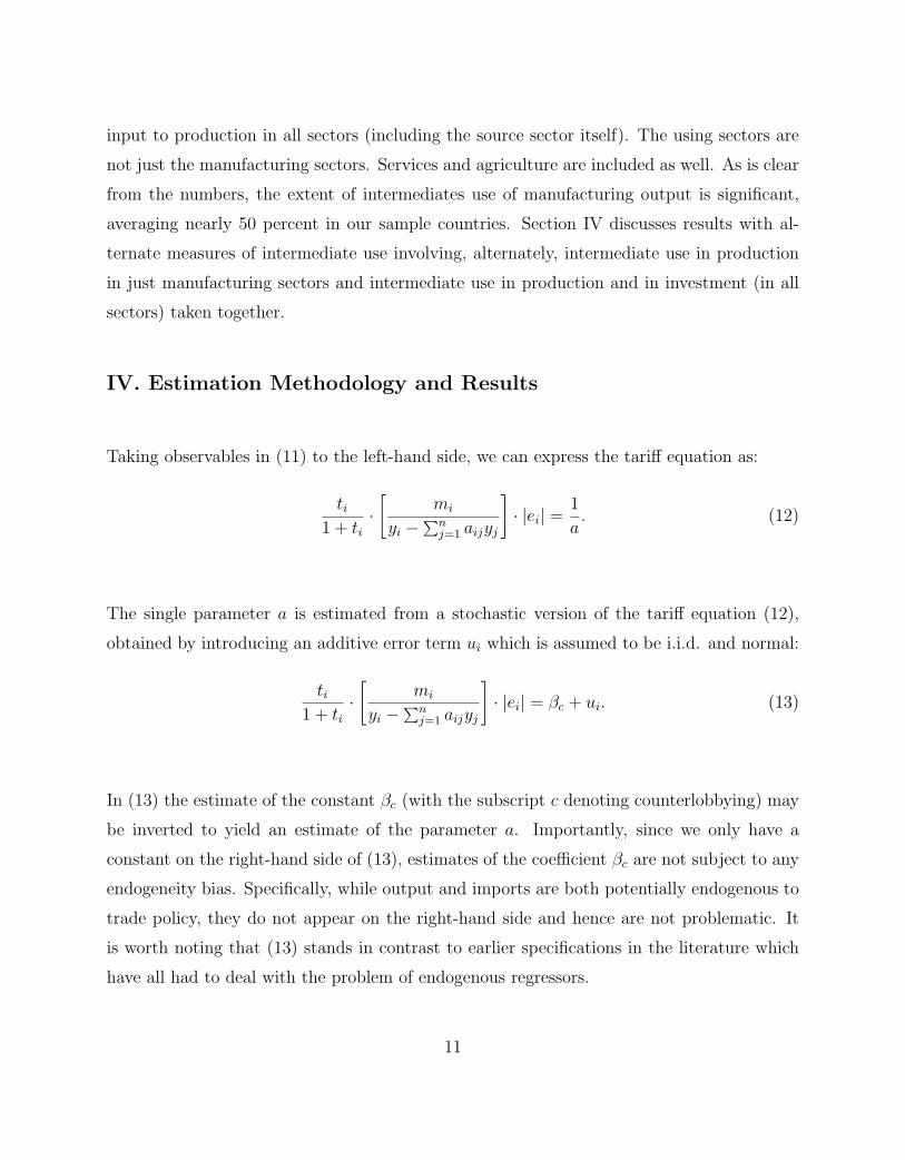
IV. Estimation Methodology and Results

Taking observables in (11) to the left-hand side, we can express the tariff equation as:

ti1 + ti

·[

mi

yi −∑n

j=1 aijyj

]· |ei| =

1

a. (12)

The single parameter a is estimated from a stochastic version of the tariff equation (12),

obtained by introducing an additive error term ui which is assumed to be i.i.d. and normal:

ti1 + ti

·[

mi

yi −∑n

j=1 aijyj

]· |ei| = βc + ui. (13)

In (13) the estimate of the constant βc (with the subscript c denoting counterlobbying) may

be inverted to yield an estimate of the parameter a. Importantly, since we only have a

constant on the right-hand side of (13), estimates of the coefficient βc are not subject to any

endogeneity bias. Specifically, while output and imports are both potentially endogenous to

trade policy, they do not appear on the right-hand side and hence are not problematic. It

is worth noting that (13) stands in contrast to earlier specifications in the literature which

have all had to deal with the problem of endogenous regressors.

11

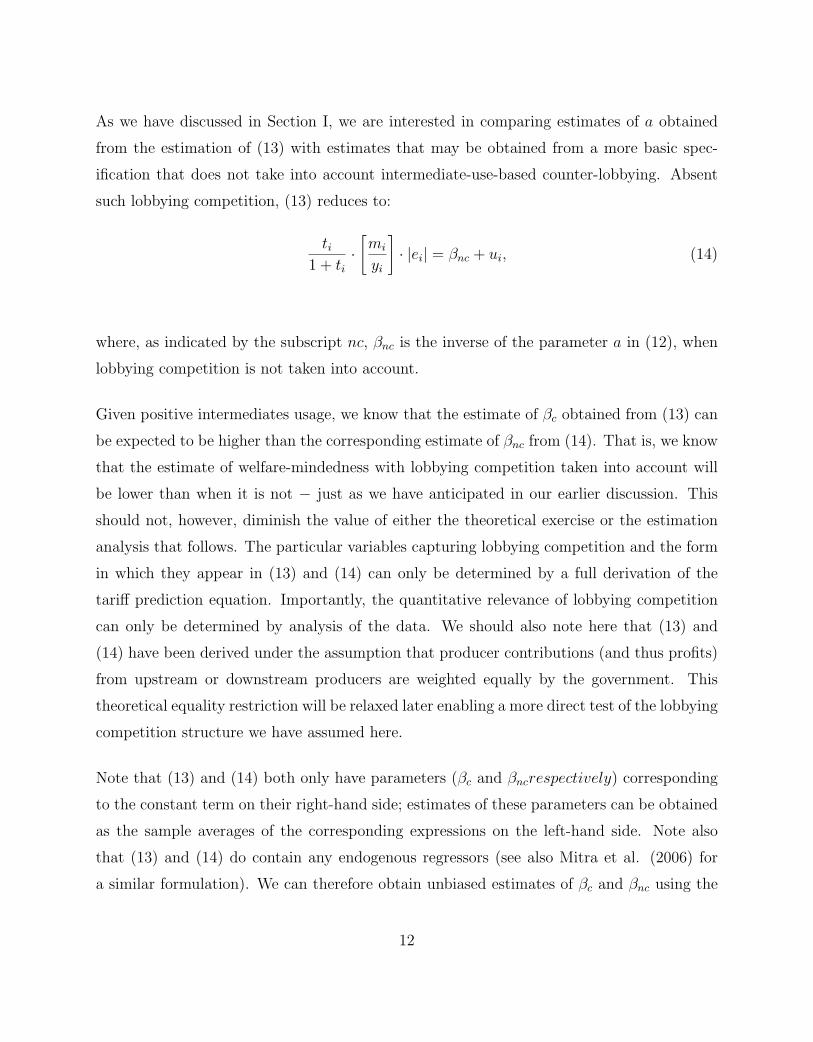
As we have discussed in Section I, we are interested in comparing estimates of a obtained

from the estimation of (13) with estimates that may be obtained from a more basic spec-

ification that does not take into account intermediate-use-based counter-lobbying. Absent

such lobbying competition, (13) reduces to:

ti1 + ti

·[mi

yi

]· |ei| = βnc + ui, (14)

where, as indicated by the subscript nc, βnc is the inverse of the parameter a in (12), when

lobbying competition is not taken into account.

Given positive intermediates usage, we know that the estimate of βc obtained from (13) can

be expected to be higher than the corresponding estimate of βnc from (14). That is, we know

that the estimate of welfare-mindedness with lobbying competition taken into account will

be lower than when it is not − just as we have anticipated in our earlier discussion. This

should not, however, diminish the value of either the theoretical exercise or the estimation

analysis that follows. The particular variables capturing lobbying competition and the form

in which they appear in (13) and (14) can only be determined by a full derivation of the

tariff prediction equation. Importantly, the quantitative relevance of lobbying competition

can only be determined by analysis of the data. We should also note here that (13) and

(14) have been derived under the assumption that producer contributions (and thus profits)

from upstream or downstream producers are weighted equally by the government. This

theoretical equality restriction will be relaxed later enabling a more direct test of the lobbying

competition structure we have assumed here.

Note that (13) and (14) both only have parameters (βc and βncrespectively) corresponding

to the constant term on their right-hand side; estimates of these parameters can be obtained

as the sample averages of the corresponding expressions on the left-hand side. Note also

that (13) and (14) do contain any endogenous regressors (see also Mitra et al. (2006) for

a similar formulation). We can therefore obtain unbiased estimates of βc and βnc using the

12

method of Ordinary Least Squares (OLS), pooling data (separately for each country) across

industries and over time (and allowing for a generalized correlation structure across the error

terms to obtain robust standard errors). Since the theoretical structure assumes a common

parameter “a” across industries, allowing for industry fixed effects in the estimation is not

really consistent with the theory. This said, within estimates (allowing for industry and/or

time fixed effects) as well as the between estimates of βc and βnc should, in principle, yield

exactly the same point estimate as those obtained with pooled OLS. This is true for the

following reason. Intuitively, with panel fixed effects in place, welfare-mindedness should be

measured as the overall average of the industry effects across time. It is easy to see that this

corresponds to the average of the left-hand side variable in (13) (and (14) in the no counter-

lobbying case) and is thus the same as the estimate obtained from pooled OLS.8 Separately,

the between estimates of the coefficient also remain the same in the presence of a balanced

panel, as the between transformation simply implies taking the mean of each industry across

time before estimating (13) or (14). In our case the panel is slightly unbalanced due to

some instances of missing data, but the point estimates are generally very close to the ones

obtained using pooled OLS and are available from us on request.

Table II presents OLS country-specific estimates of the parameters βnc and βc. As noted

above, data from over 40 different countries were used to obtain country specific estimates of

these parameters. As the numbers in Table II suggest, the estimates are highly significant for

all countries. This is true for estimates from the benchmark model (13) as well as estimates

obtained when accounting for intermediates use. The implied values of a are presented as

well.

The cross-country variation in the estimates is worth noting. Parameter estimates for, say,

Singapore, Korea and Japan are relatively low (i.e., the implied estimates of a are relatively

high). On the other hand, for Thailand, Bangladesh, Pakistan and Mexico, we obtain much

higher parameter estimates (low implied values of a). The difference in these estimates across

8Note that this corresponds exactly to the estimation routines in the statistical software STATA in whichthe sum of the fixed effects is set to zero, so that the constant term in the within regression is measured asthe overall or the grand mean (when there are no additional right-hand side variables). See ”Interpretingthe Intercept in the Fixed Effects Model” at http://www.stata.com/support/faqs/stat/xtreg2.html.

13

countries is clearly substantial. Leaving aside Singapore, which is nearly characterized by free

trade, the ratio of implied a’s in Japan and Korea are about 30 to 50 times that of countries

on the lower end such as Bangladesh, Kenya, Mexico, Pakistan, Sri Lanka and Thailand.

The cross-country variations in the implied values of a accords well with our priors regarding

the “welfare-mindedness” of governments in relation to trade policy making, thus increasing

our confidence in the data and methodology used to obtain our estimates.9

Importantly, accounting for lobbying competition changes the implied values of a systemat-

ically. In all of the sample countries, estimates of a are lowered once intermediates use is

taken into account. The magnitude of the reduction in the estimated value of a is notewor-

thy. For over 30 countries in the sample, the estimate of a is lowered to less than half its

original value once intermediates use is taken into account. We have discussed earlier how

ignoring lobbying competition may lead to incorrect estimates of the “welfare-mindedness”

of governments. Specifically, imagine that competition between lobbies leads to free trade

as an equilibrium outcome with a government that is willing to sell policy distortions cheap.

Observing the free trade outcome, but ignoring the extent of lobbying competition, may

lead an analyst to conclude − incorrectly − that policy is being set by a welfare-maximizing

government instead. The estimates presented in Table II show that introducing lobbying

competition into the analysis does indeed lower the estimate of “welfare-mindedness” of

governments and it does so significantly.

The preceding analysis suggests that the role of lobbying competition is important in un-

derstanding trade policy determination. Thus far, this conclusion has been reached by

comparing estimates of the government’s welfare-mindedness in setting trade policy with

and without counter-lobbying taken into account. Now, with some slight modifications,

we examine the role of lobbying competition more directly. Specifically, moving the terms

concerning intermediate use in production to the right-hand side, (11) may be re-written as:

9We may note that the correlation between our estimates of a and the estimates of the degree of corruptionin each country according to the Transparency International index in 2005 is 0.43. Note that not all lobbyingactivities are illegal and therefore should not be classified as “corrupt” activities.

14

ti1 + ti

· mi

yi

· |ei| =1

a

(1 −

∑nj=1 aijyj

yi

). (15)

Separating out the terms corresponding to the upstream and downstream components of

(15), we can write down the following econometric model:

ti1 + ti

· mi

yi

· |ei| = βu + βd

∑nj=1 aijyj

yi

+ ui, (16)

where ui is an i.i.d normal error term, βu > 0 denotes the parameter associated with up-

stream import-competing producers, and βd < 0 denotes the parameter associated with the

intermediate input usage terms. Note that βu 6= −βd corresponds to a theoretical formulation

in which producer contributions (and thus profits) from upstream or downstream producers

are weighted differently by the government. With βu = −βd, upstream and downstream pro-

ducers are equally weighted. Equation (16) allows us to test the validity of this theoretical

restriction.

The variable on the right-hand side of (16),

∑n

j=1aijyj

yi, is the proportion of sector i’s output

that is used as an intermediate input by other sectors. Importantly, unlike sectoral output,

which is arguably directly endogenous to sectoral trade policy, this ratio may be argued to be

determined by the technological structure of the economy and by consumption preferences,

both of which are largely exogenous. In any event, a comparison of the OLS estimates of (16)

with those obtained from (13), where regressor endogeneity is simply not a problem, enables

an evaluation of whether regressor endogeneity is a substantial issue in the estimation of

(16).

To summarize, (13) already gives us estimates of a taking counterlobbying into account and in

principle we could stop there. Equation (16) simply relaxes the equality restriction implicit

in (13) and its estimation allows us to put this restriction to test. Finally, a comparison

15

with estimates from (13) will enable an evaluation of whether regressor endogeneity is a

substantial issue in the estimation of (16).

We estimate the parameters βu and βd in (16) using pooled OLS. As we have indicated

earlier, since the theoretical structure assumes a common parameter “a” across industries,

allowing for industry fixed effects in the estimation is not really consistent with the theory. In

any case, limited variation over time in the counterlobbying variable (measured using input-

output coefficients) on the right-hand side makes the use of industry fixed effects infeasible.

For the same reason, between estimates of the parameters in (16) are quantitatively and

qualitatively very similar to those obtained by pooled OLS (and are available from us on

request).

Estimates of the parameters βu and βd in (16) and the implied values of a are reported in

Table III. βu is estimated to be greater than zero and statistically significant in nearly all

our sample countries. βd, the coefficient on the term capturing intermediates-use in (16), is

negative and significant in the majority of countries, directly affirming the role of lobbying

competition in trade policy determination. In some countries (Bangladesh, Cameroon, Costa

Rica, Hungary, Indonesia, Kenya, Mauritius, Pakistan, Peru, Romania, and Sweden), the

direct evidence on counterlobbying is statistically weaker, but even for these countries the

point estimates are in the theoretically correct direction. Note that values of a may be

inferred from either estimated coefficient. In general, the magnitude of the absolute values

of βu and βd are very close to each other (even though F-tests reject the null of equality in a

significant minority of the cases), so that the implied value of a does not vary substantially

with the coefficient used. We report values of a implied by 1/βu. Table III indicates, once

again, high values of a for Singapore, Japan, Korea, and low values for Bangladesh, Pakistan

and Mexico. As with the results reported in Table II, the estimates sit fairly well with our

priors regarding the “welfare-mindedness” of these respective countries. The implied values

of a in Table III correlate highly with those reported in Table II. As discussed earlier, this

mitigates our concern regarding regressor endogeneity.

Robustness

16

The robustness of our empirical findings was evaluated in a number of ways. First, we

conducted the entire analysis using additional measures of intermediates use: the percentage

of a source sector’s output that is used in the manufacturing sectors of the economy and,

separately, the percentage of a source sector’s output that is used as intermediate input by

all producing sectors in the economy plus what is used in final investment spending. The

former is a less comprehensive and the latter a more comprehensive measure than those

used in obtaining the results presented in Tables II and III, resulting in somewhat larger

and smaller estimates of a respectively. This is as expected since these measures introduce,

in turn, counter-lobbying by less and more users respectively. Otherwise there is little

qualitative change in the results with the use of these alternate measures of intermediates

use. The range of estimates is close to the results we report, as is the ranking of countries

by a. These results are available from us on request.

V. Conclusions

Competition between opposing lobbies is a potentially important factor in the endogenous

determination of trade policy. This paper has investigated the consequences of such lobbying

competition for trade policy. The theoretical framework we have used for our empirical

analysis is the well-known Grossman-Helpman model of trade policy determination suitably

modified to account for the cross-sectoral use of inputs in production (the input-output

matrix). Our empirical results, using trade and protection data from over 40 high- middle-

and low-income countries, validate the predictions of the theoretical model with lobbying

competition. The presence of organized downstream users of an industry’s output is found

to reduce trade protection.10

10Other recent extensions of the theory have also improved the empirical fit of the model. See, forinstance, Matschke and Sherlund (2006), who introduce labor market factors into the analysis, Freund andOzden (2005), who consider the implications for trade policy of “loss aversion” behavior on the part oflobbyists, Bombardini (2005), who considers empirically the implications of endogenous lobby formation asin the important model of Mitra (1999), and Facchini et al. (2006), who introduce imperfect rent-capturing.

17

References

Bombardini, M., 2005, “Firm Heterogeneity and Lobby Participation,” Mimeo, MIT.

Cadot, O., de Melo, J., and Olarreaga, M., 2003, “The Protectionist Bias of Duty Drawbacks:Evidence From Mercosur,” Journal of International Economics, 59, pp 161-182.

Duttagupta, R., and Panagariya, A., 2003, “Free Trade Areas and Rules of Origin: Economics andPolitics,” IMF Working Papers, 03/229, International Monetary Fund.

Eicher, T. and Osang, T., 2002,“Protection for Sale: An Empirical Investigation: Comment,”American Economic Review 92: 1702-1710.

Facchini, G., Van Biesebroeck, J., and Willmann. G., 2006, “Protection for Sale with ImperfectRent Capturing,” Canadian Journal of Economics, 39:845-873.

Freund, C., and Ozden, C., 2005, “Loss Aversion and Trade Policy,” Policy Research WorkingPaper, Number 3385, World Bank.

Gawande, K., and Bandyopadhyay, U., 2000, “Is Protection for Sale? A Test of the Grossman-Helpman Theory of Endogenous Protection”, Review of Economics and Statistics, 89: 139-152.

Goldberg, P., and Maggi, G., 1999, “Protection for Sale: An Empirical Investigation”, AmericanEconomic Review, 89: 1135-1155.

Grossman, G. and Helpman, E., 1994, “Protection for Sale”, American Economic Review, 84:833-850.

Kee, H. L. , Nicita A., and Olarreaga, M., 2008, “Import Demand Elasticities and Trade Distor-tions,”Review of Economics and Statistics. Forthcoming.

McCalman, P, 2004, “Protection for Sale and Trade Liberalization: An Empirical Investigation,”Review of International Economics 12: 8194.

Matschke, Z. and Sherlund, S., 2006, “Do Labor Issues Matter in the Determination of TradePolicy? An Empirical Re-Evaluation,” American Economic Review, 96: 405-421

Mitra, D., 1999, “Endogenous Lobby Formation and Endogenous Protection: A Long-Run Modelof Trade Policy Determination,” American Economic Review, 89: 1116-1134.

Mitra, D., Thomakos, D., and Ulubasoglu, M., 2006, “Can we Obtain Realistic Estimates for the‘Protection For Sale’ Model?”, Canadian Journal of Economics, 39: 187-210

18

Olson, M., 1965, The Logic of Collective Action, Harvard University Press, Cambridge: MA

19

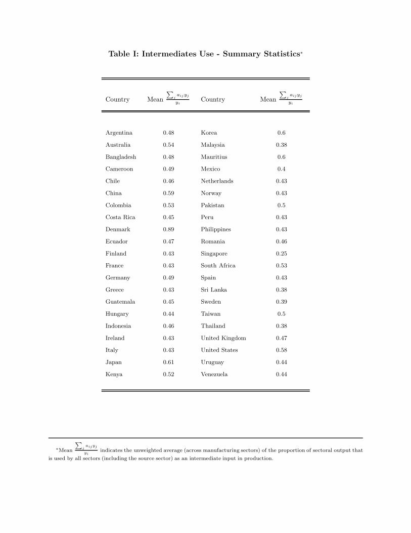
Table I: Intermediates Use - Summary Statistics∗

Country Mean∑

jaijyj

yiCountry Mean

∑j

aijyj

yi

Argentina 0.48 Korea 0.6

Australia 0.54 Malaysia 0.38

Bangladesh 0.48 Mauritius 0.6

Cameroon 0.49 Mexico 0.4

Chile 0.46 Netherlands 0.43

China 0.59 Norway 0.43

Colombia 0.53 Pakistan 0.5

Costa Rica 0.45 Peru 0.43

Denmark 0.89 Philippines 0.43

Ecuador 0.47 Romania 0.46

Finland 0.43 Singapore 0.25

France 0.43 South Africa 0.53

Germany 0.49 Spain 0.43

Greece 0.43 Sri Lanka 0.38

Guatemala 0.45 Sweden 0.39

Hungary 0.44 Taiwan 0.5

Indonesia 0.46 Thailand 0.38

Ireland 0.43 United Kingdom 0.47

Italy 0.43 United States 0.58

Japan 0.61 Uruguay 0.44

Kenya 0.52 Venezuela 0.44

∗Mean

∑j

aijyj

yiindicates the unweighted average (across manufacturing sectors) of the proportion of sectoral output that

is used by all sectors (including the source sector) as an intermediate input in production.

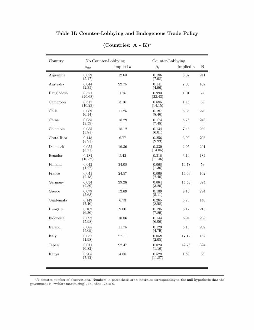
Table II: Counter-Lobbying and Endogenous Trade Policy

(Countries: A - K)∗

Country No Counter-Lobbying Counter-Lobbyingβnc Implied a βc Implied a N

Argentina 0.079 12.63 0.186 5.37 241(5.17) (7.98)

Australia 0.044 22.75 0.141 7.08 162(2.35) (4.96)

Bangladesh 0.571 1.75 0.993 1.01 74(20.68) (22.43)

Cameroon 0.317 3.16 0.685 1.46 59(10.23) (14.15)

Chile 0.089 11.25 0.187 5.36 270(6.14) (8.46)

China 0.055 18.29 0.174 5.76 243(3.59) (7.48)

Colombia 0.055 18.12 0.134 7.46 269(3.81) (6.01)

Costa Rica 0.148 6.77 0.256 3.90 205(8.91) (9.93)

Denmark 0.052 19.36 0.339 2.95 291(3.71) (14.05)

Ecuador 0.184 5.43 0.318 3.14 184(10.52) (11.46)

Finland 0.042 24.08 0.068 14.78 53(1.27) (1.36)

France 0.041 24.57 0.068 14.63 162(2.18) (2.40)

Germany 0.034 29.28 0.064 15.53 324(2.59) (3.20)

Greece 0.079 12.69 0.109 9.16 294(5.68) (5.11)

Guatemala 0.149 6.73 0.265 3.78 140(7.40) (8.58)

Hungary 0.102 9.80 0.195 5.12 215(6.30) (7.89)

Indonesia 0.092 10.86 0.144 6.94 238(5.98) (6.06)

Ireland 0.085 11.75 0.123 8.15 202(5.09) (4.79)

Italy 0.037 27.11 0.058 17.12 162(1.98) (2.05)

Japan 0.011 92.47 0.023 42.76 324(0.82) (1.16)

Kenya 0.205 4.88 0.529 1.89 68(7.12) (11.87)

∗N denotes number of observations. Numbers in parenthesis are t-statistics corresponding to the null hypothesis that thegovernment is “welfare maximizing”, i.e., that 1/a = 0.

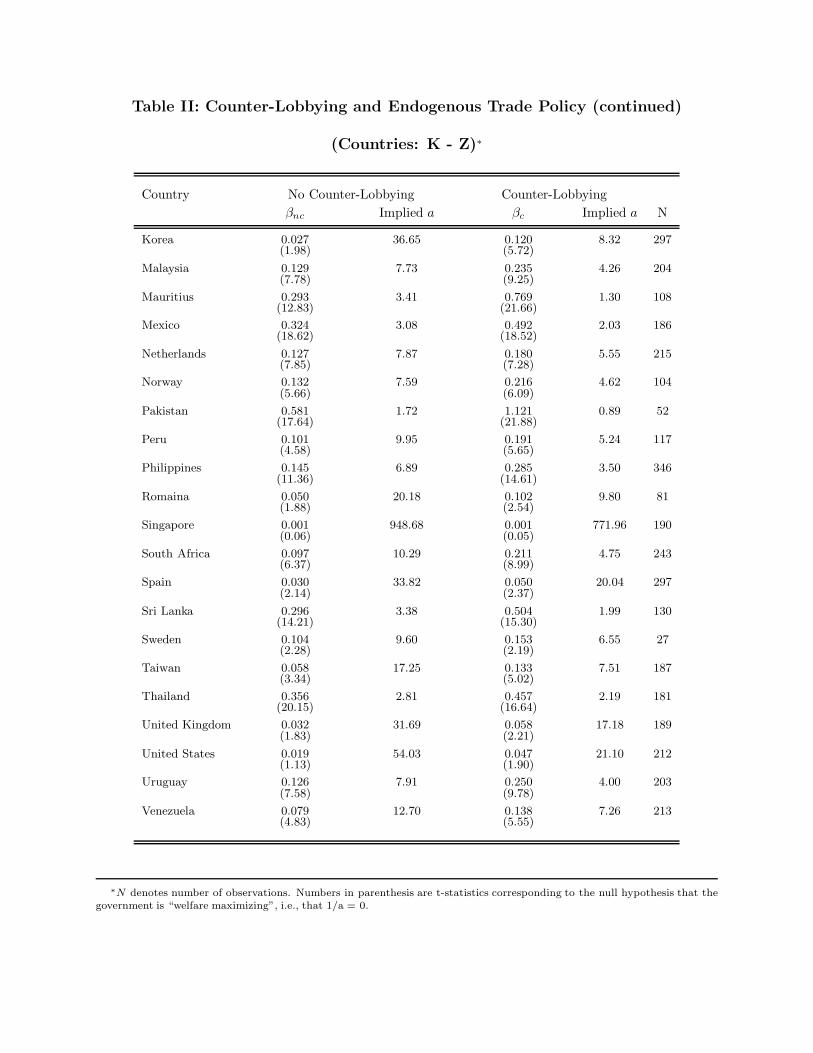
Table II: Counter-Lobbying and Endogenous Trade Policy (continued)

(Countries: K - Z)∗

Country No Counter-Lobbying Counter-Lobbyingβnc Implied a βc Implied a N

Korea 0.027 36.65 0.120 8.32 297(1.98) (5.72)

Malaysia 0.129 7.73 0.235 4.26 204(7.78) (9.25)

Mauritius 0.293 3.41 0.769 1.30 108(12.83) (21.66)

Mexico 0.324 3.08 0.492 2.03 186(18.62) (18.52)

Netherlands 0.127 7.87 0.180 5.55 215(7.85) (7.28)

Norway 0.132 7.59 0.216 4.62 104(5.66) (6.09)

Pakistan 0.581 1.72 1.121 0.89 52(17.64) (21.88)

Peru 0.101 9.95 0.191 5.24 117(4.58) (5.65)

Philippines 0.145 6.89 0.285 3.50 346(11.36) (14.61)

Romaina 0.050 20.18 0.102 9.80 81(1.88) (2.54)

Singapore 0.001 948.68 0.001 771.96 190(0.06) (0.05)

South Africa 0.097 10.29 0.211 4.75 243(6.37) (8.99)

Spain 0.030 33.82 0.050 20.04 297(2.14) (2.37)

Sri Lanka 0.296 3.38 0.504 1.99 130(14.21) (15.30)

Sweden 0.104 9.60 0.153 6.55 27(2.28) (2.19)

Taiwan 0.058 17.25 0.133 7.51 187(3.34) (5.02)

Thailand 0.356 2.81 0.457 2.19 181(20.15) (16.64)

United Kingdom 0.032 31.69 0.058 17.18 189(1.83) (2.21)

United States 0.019 54.03 0.047 21.10 212(1.13) (1.90)

Uruguay 0.126 7.91 0.250 4.00 203(7.58) (9.78)

Venezuela 0.079 12.70 0.138 7.26 213(4.83) (5.55)

∗N denotes number of observations. Numbers in parenthesis are t-statistics corresponding to the null hypothesis that thegovernment is “welfare maximizing”, i.e., that 1/a = 0.

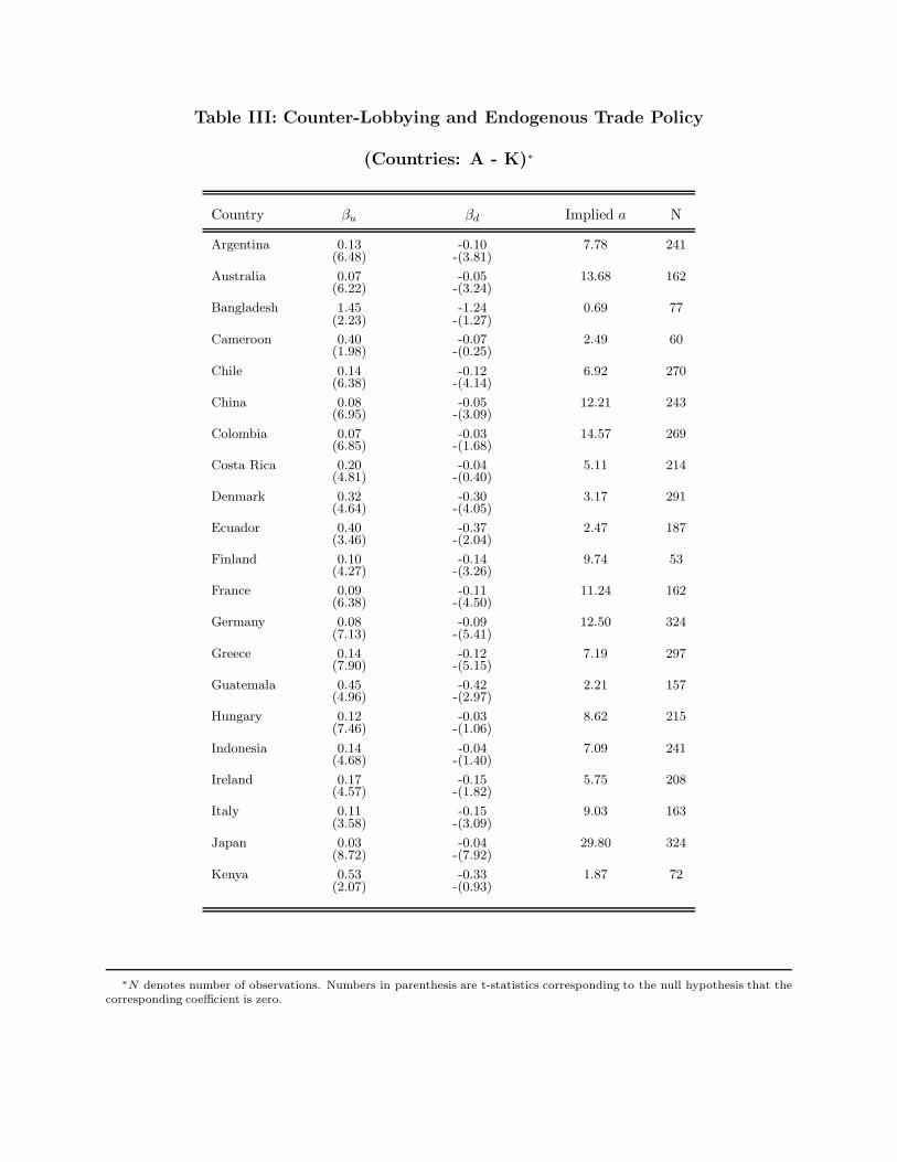
Table III: Counter-Lobbying and Endogenous Trade Policy

(Countries: A - K)∗

Country βu βd Implied a N

Argentina 0.13 -0.10 7.78 241(6.48) -(3.81)

Australia 0.07 -0.05 13.68 162(6.22) -(3.24)

Bangladesh 1.45 -1.24 0.69 77(2.23) -(1.27)

Cameroon 0.40 -0.07 2.49 60(1.98) -(0.25)

Chile 0.14 -0.12 6.92 270(6.38) -(4.14)

China 0.08 -0.05 12.21 243(6.95) -(3.09)

Colombia 0.07 -0.03 14.57 269(6.85) -(1.68)

Costa Rica 0.20 -0.04 5.11 214(4.81) -(0.40)

Denmark 0.32 -0.30 3.17 291(4.64) -(4.05)

Ecuador 0.40 -0.37 2.47 187(3.46) -(2.04)

Finland 0.10 -0.14 9.74 53(4.27) -(3.26)

France 0.09 -0.11 11.24 162(6.38) -(4.50)

Germany 0.08 -0.09 12.50 324(7.13) -(5.41)

Greece 0.14 -0.12 7.19 297(7.90) -(5.15)

Guatemala 0.45 -0.42 2.21 157(4.96) -(2.97)

Hungary 0.12 -0.03 8.62 215(7.46) -(1.06)

Indonesia 0.14 -0.04 7.09 241(4.68) -(1.40)

Ireland 0.17 -0.15 5.75 208(4.57) -(1.82)

Italy 0.11 -0.15 9.03 163(3.58) -(3.09)

Japan 0.03 -0.04 29.80 324(8.72) -(7.92)

Kenya 0.53 -0.33 1.87 72(2.07) -(0.93)

∗N denotes number of observations. Numbers in parenthesis are t-statistics corresponding to the null hypothesis that thecorresponding coefficient is zero.

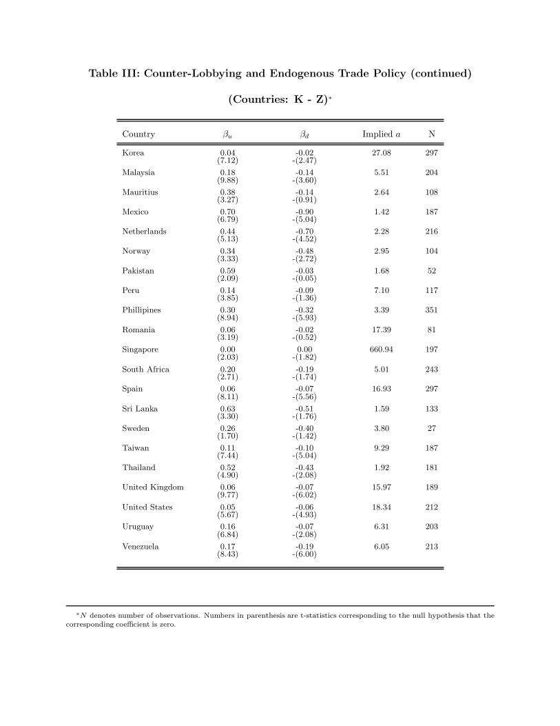
Table III: Counter-Lobbying and Endogenous Trade Policy (continued)

(Countries: K - Z)∗

Country βu βd Implied a N

Korea 0.04 -0.02 27.08 297(7.12) -(2.47)

Malaysia 0.18 -0.14 5.51 204(9.88) -(3.60)

Mauritius 0.38 -0.14 2.64 108(3.27) -(0.91)

Mexico 0.70 -0.90 1.42 187(6.79) -(5.04)

Netherlands 0.44 -0.70 2.28 216(5.13) -(4.52)

Norway 0.34 -0.48 2.95 104(3.33) -(2.72)

Pakistan 0.59 -0.03 1.68 52(2.09) -(0.05)

Peru 0.14 -0.09 7.10 117(3.85) -(1.36)

Phillipines 0.30 -0.32 3.39 351(8.94) -(5.93)

Romania 0.06 -0.02 17.39 81(3.19) -(0.52)

Singapore 0.00 0.00 660.94 197(2.03) -(1.82)

South Africa 0.20 -0.19 5.01 243(2.71) -(1.74)

Spain 0.06 -0.07 16.93 297(8.11) -(5.56)

Sri Lanka 0.63 -0.51 1.59 133(3.30) -(1.76)

Sweden 0.26 -0.40 3.80 27(1.70) -(1.42)

Taiwan 0.11 -0.10 9.29 187(7.44) -(5.04)

Thailand 0.52 -0.43 1.92 181(4.90) -(2.08)

United Kingdom 0.06 -0.07 15.97 189(9.77) -(6.02)

United States 0.05 -0.06 18.34 212(5.67) -(4.93)

Uruguay 0.16 -0.07 6.31 203(6.84) -(2.08)

Venezuela 0.17 -0.19 6.05 213(8.43) -(6.00)

∗N denotes number of observations. Numbers in parenthesis are t-statistics corresponding to the null hypothesis that thecorresponding coefficient is zero.