Lidar monitoring of regions of intense backscatterwith poorly defined boundaries

Vladimir A. Kovalev,* Alexander Petkov, Cyle Wold, and Wei Min HaoUnited States Forest Service, RMRS, Fire Sciences Laboratory, 5775 Highway 10 West, Missoula, Montana, 59808, USA

*Corresponding author: vkovalev@fs.fed.us

Received 31 August 2010; accepted 7 November 2010;posted 19 November 2010 (Doc. ID 134285); published 27 December 2010

The upper height of a region of intense backscatter with a poorly defined boundary between this regionand a region of clear air above it is found as the maximal height where aerosol heterogeneity is detect-able, that is, where it can be discriminated from noise. The theoretical basis behind the retrieval tech-nique and the corresponding lidar-data-processing procedures are discussed. We also show how such atechnique can be applied to one-directional measurements. Examples of typical results obtained with ascanning lidar in smoke-polluted atmospheres and experimental data obtained in an urban atmospherewith a vertically pointing lidar are presented. © 2010 Optical Society of AmericaOCIS codes: 280.3640, 290.1350, 290.2200.

1. Introduction

There is no commonly accepted technique for remotemonitoring of the locations and temporal and spatialchanges of regions of increased backscatter withpoorly defined boundaries, such as those that arefound in dispersed smoke plumes originating in wild-fires, dust clouds, or aerosol clouds created by volca-no eruptions.

To monitor the behavior of intense backscatterregions in the atmosphere, lidar is the most appro-priate tool. In principle, lidar can easily detect theboundary between different atmospheric layersand discriminate the regions with high levels of back-scatter from the regions of clear atmosphere. Well-defined heterogeneous areas, such as the atmo-spheric boundary layer or clouds, can be identifiedthrough the visual inspection of the lidar scan andis a trivial matter [1]. However, the identificationof the exact location of the boundary of a heteroge-neous structure becomes a significant challengewhen the boundary is not well defined. Such a situa-tion is typical, for example, for smoke layers andplumes where the dispersion processes create a

continuous transition zone between the intensebackscatter region and clear air. The smoke plumedensity, its concentrations, the levels of the heteroge-neity, and the smoke dispersion are extremely vari-able and depend heavily on the distance from thesmoke plume source.

The absence of unique criteria for determining theboundary between the increased-backscatter andclear-air areas when it is not well defined is the prin-cipal issue when using any range-resolved remotesensing technique. This challenge is a general pro-blem rather than a problem of remote-sensing meth-odology. No standard definition of such a boundaryexists. When determining the boundaries of the aero-sol formation, generally, some relative rather thanabsolute characteristics are used. For example, whenusing a gradient method, one can select the boundarylocation as the range where the examined parameterof interest (e.g., the derivative of the square-range-corrected lidar signal) is a maximum or decreasesfrom the maximum value down to a fixed, user-defined level [2]. However, there is no way to estab-lish a standard value for this level, which would beacceptable for all cases of atmospheric searching. Si-milarly, the use of the wavelet technique requires theselection of concrete parameters, and this is a signif-icant challenge when a region of intense backscatter

0003-6935/11/010103-07$15.00/0© 2011 Optical Society of America

1 January 2011 / Vol. 50, No. 1 / APPLIED OPTICS 103

with a poorly defined boundary is examined [3]. Inthis study, an alternative approach to this issue isconsidered.

2. Methodology

The lidar signal, PΣðrÞ, recorded at the range r, is thesum of the range-dependent backscatter signal,PðrÞ and the range-independent offset, B, the back-ground component of the lidar signal and the electro-nic offset:

PΣðrÞ ¼ PðrÞ þ B: ð1ÞThis signal is transformed in the auxiliary functionYðxÞ, defined as [4]

YðxÞ ¼ PΣðxÞx ¼ ½PðxÞ þ B�x; ð2Þwhere x ¼ r2 is the new independent variable. In thecurrent study, we apply the simplest form of thetransformation, which does not require the use ofthe molecular profile of the searched atmosphere.The sliding derivative of this function, dY=dx, is cal-culated, and the intercept point of each local slope fitof the function with the vertical axis is found and nor-malized. The intercept function versus x is found as

Y0ðxÞ ¼ YðxÞ − dYdx

x: ð3Þ

By using the intercept function instead of dY=dx, thedetermination of the systematic offset, B, in the lidarsignal [Eq. (1)] can be avoided. The retrieval tech-nique that is used here for processing the signalsof both scanning and one-directional lidar is basedon determining the normalized intercept function[4]. The normalized intercept function is defined as

Y0;normðxÞ ¼Y0ðxÞ

xþ εxmax; ð4Þ

where xmax is the maximum value of the variable xover the selected range and ε is a positive nonzeroconstant, whose value can range from 0.02–0.05.The selection of the numerical value for ε is not cri-tical. The component εxmax in the denominator of theequation is included only to suppress the excessiveincrease of Y0;normðxÞ in the region of small x, which,for our task, is not the region of interest. Note alsothat the numerical differentiation in Eq. (3) is madewith a constant step, Δr ¼ riþ1 − ri ¼ const:, ratherthan a constant Δx. Under such a condition, the stepΔx is variable, that is,

Δx ¼ r2iþ1 − r2i ¼ Δr2�1þ 2ri

Δr

�: ð5Þ

In this paper, we restrict our analysis to the determi-nation of the maximum heights of the regions of theincreased backscatter; the determination of the mini-mum heights, especially in a multilayering atmo-

sphere, is a much more complicated task andrequires separate consideration.

A. Determination of the Maximal Height of the Region ofIncreased Backscatter Using Scanning Lidar

Consider the case where lidar scanning is performedin a fixed azimuthal direction, θ, using Nφ slope di-rections selected within the angular sector from φminto φmax and with the stepped angular resolution ofΔφ; that is, φ1 ¼ φmin, φ2 ¼ φmin þΔφ;…, φi ¼φmin þ ði − 1ÞΔφ;…, and φN ¼ φmax. The recordedsignals, measured within the range from rmin tormax, are transformed into the corresponding set ofthe normalized functions, Y0;normðhÞ, versus height,h; these functions are calculated within the altituderange from hmin to hmax with the selected height re-solution, Δh; that is, h1 ¼ hmin, h2 ¼ hmin þΔh;…,hj ¼ hmin þ ðj − 1ÞΔh;…, and hM ¼ hmax; M is thenumber of heights within the selected interval½hmin;hmax�.

To locate the maximum height of the region of in-creased backscatter, the absolute values of the nor-malized intercept function versus height for eachslope direction φi and each hj within the altituderange from hmin to hmax, are calculated:

f i;j ¼ jY0;normðφi;hjÞj: ð6Þ

Thus, for our calculations we define the matrix Fφ,with matrix elements f i;j ∈ ðNφ;MÞ; that is, Fφ ¼½f i;j�NφHM. The maximum matrix element, fmax ¼max½f i;j�Nφ×M , is determined and the matrix isnormalized:

Rφ ¼ 1fmax

Fφ: ð7Þ

The elements of the matrix, ri;j ¼ Rðφj;hjÞ, which areused for determining the areas of the smoke plume,can vary within the range 0 ≤ ri;j ≤ 1, with areas ap-proaching ri;j ¼ 1 having the greatest heterogeneity.

In our original study [4], the local “heterogeneityevent” defined in two-dimensional space ði; jÞwas im-plemented. The event was considered as being trueat the locations where the elements ri;j of the matrixFφ reach some established, user-defined level, χ < 1.In other words, we supposed that the atmosphericheterogeneity in the cell ði; jÞ, exists if the element,ri;j ≥ χ; in the study [4], the user-defined constant χwas selected within the range from 0.15 to 0.3. Somemodification in selecting χ was considered in [5].

To clarify the modified methodology for the deter-mination of the maximal height of the smoke-polluted area and the principle for the selection ofχ in this study, let us consider typical experimentaldata. The data were obtained by a scanning lidarin the vicinity of the Kootenai Creek Fire near Mis-soula, Montana, USA in 2009. The wildfire occurredin a wild mountainous area from which the smokeplume spread in an easterly direction across thevalley where the lidar was located. The height of

104 APPLIED OPTICS / Vol. 50, No. 1 / 1 January 2011

the lidar site was approximately 900 m below theheight of the wildfire area. The schematic of the scan-ning lidar setup is shown in Fig. 1. Lidar verticalscans were made along 23 azimuthal directions, fromθ ¼ 45° to θ ¼ 155°, with an angular incrementΔθ ¼ 5°. Thus, each scan was used to obtain a verti-cal cross-section of attenuated backscatter in the cor-responding azimuthal direction.

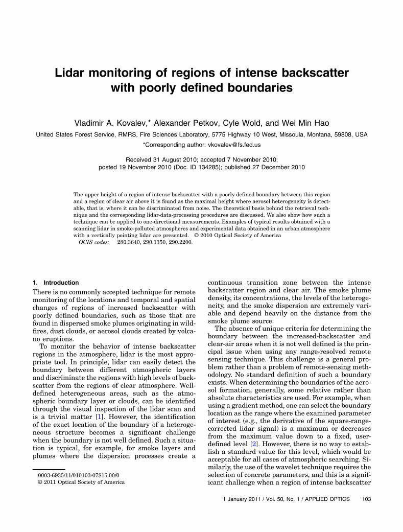
In Figs. 2–5, we clarify the details of our data-processing methodology using the results obtainedon 27 August 2009. The vertical scan analyzed belowwas made at the azimuthal direction, θ ¼ 55°, withinthe vertical angular sector from φmin ¼ 10° to φmax ¼60°; the total number of slope directions is Nφ ¼ 28.In Fig. 2, the corresponding 28 functions, Rðφi;hjÞ,are shown as the gray curves, with the thick blackcurve representing the resulting heterogeneity func-tion, Rθ;maxðhÞ, defined for each altitude as

Rθ;maxðhÞ ¼ max½Rðφ1;hÞ;Rðφ2;hÞ;…;

× Rðφi;hÞ;…;RðφN ;hÞ�: ð8Þ

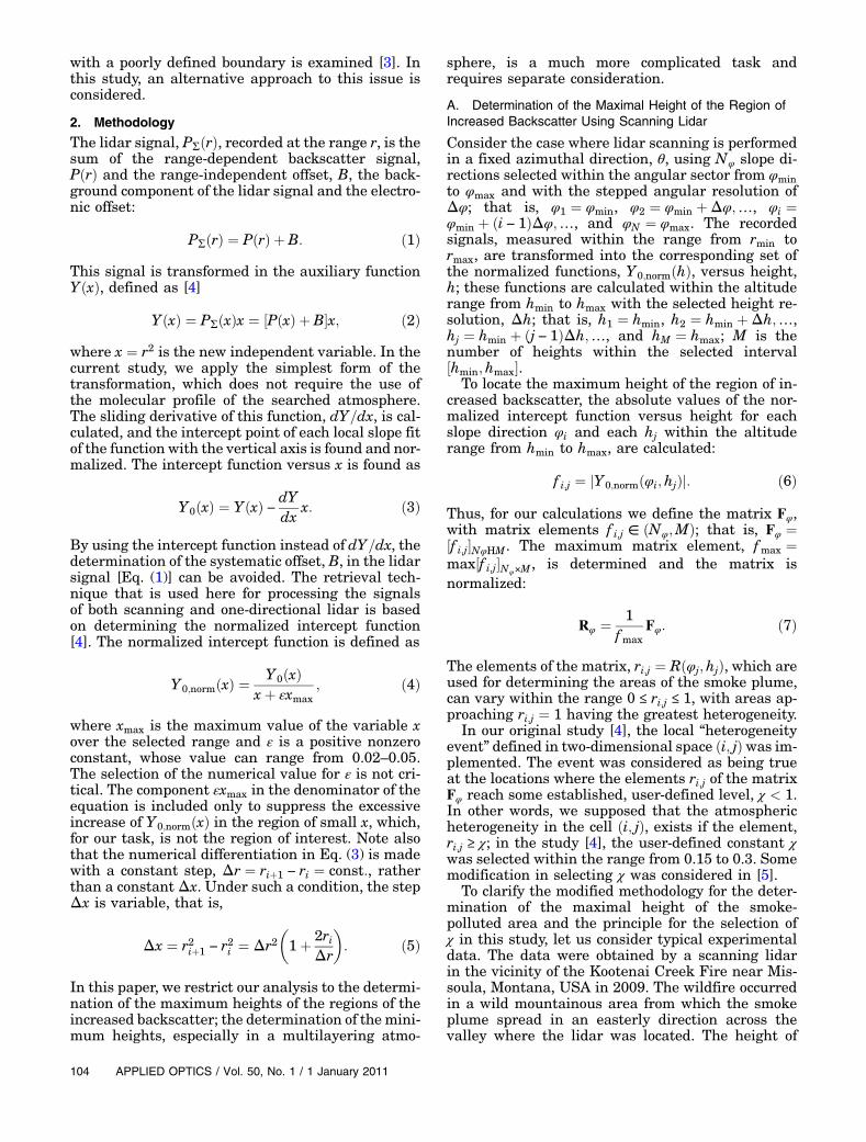
To determine the maximum height of the smoke-polluted region, the parameter, χ, can be selectedand compared to Rθ;maxðhÞ. The maximum smokeplume height, hsm;max, can be found as the maximumheight where Rθ;maxðhÞ ¼ χ. The main issue of suchan approach is the rational selection of χ. In the caseof a poorly defined boundary, the retrieved height ofthe smoke plume strongly depends on the selected χ.This observation is illustrated in Fig. 3, where theRθ;maxðhÞ shown in Fig. 2 is analyzed. One can seethat selecting different χ yields different heights ofinterest, hsm;max. For example, changing χ from 0.1to 0.15 decreases the retrieved height hsm;max from4581 to 3078 m.

Analyzing possible retrieval techniques, we con-cluded that the optimal solution could be achievedby taking advantage of the principles used for deter-mining the cloud base height when the ceiling has nowell-defined lower boundary. In such a case, thecloud base height is considered as the lowest level

of the atmosphere where cloud properties are detect-able [6]. In our study, the analogous definition isused for determining the maximum smoke plumeheight. Particularly, the upper smoke plume bound-ary height, hsm;max, can be defined as the maximumheight where smoke plume aerosols are detectable inthe presence of the noise component in the examinedfunction. This approach requires reliably distin-guishing the ri;j increases caused by the presenceof the actual smoke plume heterogeneity from thatof random noise fluctuations.

To apply the above definition in the smoke plumemeasurements, the following methodology was cho-sen. Using the retrieved functions, Rθ;maxðhÞ (Fig. 2),the atmospheric heterogeneity height indicator(AHHI) for this azimuth θ is determined. The AHHI

Fig. 1. Schematic of data collection with a vertically scanning li-dar during the Kootenai Creek Fire inMontana in July andAugust2009. (The azimuthal sector 45° − 65°, which overlaps the wildfiresite, is not shown in this figure.)

Fig. 2. Example of data obtained by a scanning lidar at the wa-velength of 1064 nm in the smoke-polluted atmosphere inthe vicinity of Missoula, Montana. The gray curves representthe set of 28 functions, Rðφi;hjÞ. The resulting heterogeneity func-tion, Rθ;maxðhÞ, is shown as the thick black curve.

Fig. 3. Black curve is the same heterogeneity function, Rθ;maxðhÞ,as in Fig. 2, and the gray blocks illustrate thedependence of the retrieved smoke plume height, hsm;max, on theselected χ.

1 January 2011 / Vol. 50, No. 1 / APPLIED OPTICS 105

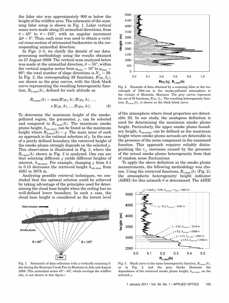
is a histogram that shows the total number of hetero-geneity events, nðhÞ, defined by scanning lidar at theconsecutive height intervals for the selected χ [4].The concept of the AHHI histogram is explained inFig. 4. The thick black curve on the left side of thefigure is the function Rθ;maxðhÞ, the same as inFigs. 2 and 3. The AHHI derived with the levelχ ¼ 0:15, is shown as black–gray squares. The max-imal height, where the minimal number of theheterogeneity events exceeds zero ½nðhÞ ¼ 1�, ishsm;max ¼ 3078 m. Note also that a maximumnumber of heterogeneity events was fixed over thealtitude range 1000 m–1150 m (n ¼ 28) and2350–2550 m (n ¼ 22), so that two separate layersat different heights can be discriminated withthe AHHI.

Using such AHHI histograms, one can determinethe maximal heights of the area with the increasedheterogeneity for different χ. In our calculations, weutilize the consecutive values of χ with the fixed stepΔχ; that is, χ0 ¼ 0, χ1 ¼ Δχ, χ2 ¼ 2Δχ;…, andχk ¼ kΔχ;…. For each discrete χ, we build the AHHIand determine the corresponding maximum height,hsm;maxðχÞ, that is, the maximum height where thenumber of heterogeneity events, nðhÞ, is a nonzerointeger value.

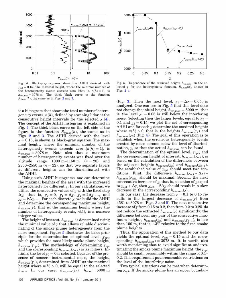
The height of interest, hsm;max, is determined usingthe minimal value of χ that allows reliable discrimi-nating of the smoke plume heterogeneity from thenoise component. Figure 5 illustrates the basic prin-ciple for the determination of optimal level, χopt,which provides the most likely smoke plume height,hsm;maxðχoptÞ. The methodology of determining χoptand the corresponding hsm;maxðχoptÞ is as follows. In-itially, the level χ0 ¼ 0 is selected. Because of the pre-sence of nonzero instrumental noise, the height,hsm;maxðχ0Þ, determined from AHHI as the maximalheight where nðhÞ > 0, will be equal to the selectedhmax. In our case, hsm;maxðχ0Þ ¼ hmax ¼ 5000 m

(Fig. 3). Then the next level, χ1 ¼ Δχ ¼ 0:05, isanalyzed. One can see in Fig. 5 that this level doesnot change the initial height, hsm;max ¼ 5000 m, thatis, the level χ1 ¼ 0:05 is still below the interferingnoise. Selecting then the larger levels, equal to χ2 ¼0:1 and χ3 ¼ 0:15, we plot the set of correspondingAHHI and for each χ determine the maximal heightswhere nðhÞ > 0, that is, the heights hsm;maxðχ2Þ andhsm;maxðχ3Þ (Fig. 5). The goal of this operation is toestablish when the erroneous heterogeneity eventscreated by noise become below the level of discrimi-nation, χ, so that the actual hsm;max can be found.

The determination of the optimal level, χopt, andthe corresponding height of interest, hsm;maxðχoptÞ, isbased on the calculation of the differences betweenthe adjacent heights hsm;maxðχkÞ and hsm;maxðχkþ1Þ.The established value of χopt should meet two con-ditions. First, the difference hsm;maxðχopt −ΔχÞ −hsm;maxðχoptÞ should be maximal. Second, the nextconsecutive increase of χ, that is, selection of χ equalto χopt þΔχ, then χopt þ 2Δχ should result in a slowdecrease in the corresponding hsm;maxðχÞ.

In our case, the decrease from χ ¼ 0:1 to 0.15 re-sults in the largest decrease of hsm;maxðχÞ from4581 to 3078 m (Figs. 3 and 5). The next consecutiveincrease of χ from 0.15 to 0.2, then from 0.2 to 0.25. donot reduce the extracted hsm;maxðχÞ significantly; thedifference between any pair of the consecutive max-imum heights, hsm;maxðχkÞ and hsm;maxðχkþ1Þ, is lessthan 100 m, that is, ∼3% relative to the fixed smokeplume heights.

Thus, the application of this method to our datayields the optimal level, χopt ¼ 0:15 and the corre-sponding hsm;maxðχoptÞ ¼ 3078 m. It is worth alsoworth mentioning that to avoid significant underes-timating the smoke plume maximum height, the χoptshould be small, presumably within the range of 0.1–0.2. This requirement puts reasonable restrictions onthe level of the interfering noise.

Two typical situations can be met when determin-ing χopt. If the smoke plume has an upper boundary

Fig. 4. Black-gray squares show the AHHI derived withχopt ¼ 0:15. The maximal height, where the minimal number ofthe heterogeneity events exceeds zero [that is, nðhÞ ¼ 1], ishsm;max ¼ 3078 m. The thick black curve is the functionRθ;maxðhÞ, the same as in Figs. 2 and 3.

Fig. 5. Dependence of the retrieved height, hsm;max, on the se-lected χ for the heterogeneity function, Rθ;maxðhÞ, shown inFigs. 2–4.

106 APPLIED OPTICS / Vol. 50, No. 1 / 1 January 2011

with no local layering in its vicinity, both require-ments are met: the systematic difference betweenthe heights, determined with the consecutive levels,χopt, χopt þΔχ;…, χopt þ 2Δχ;…, is small, whereasthe difference between the heights, determined withthe level, χopt and the previous level, χopt −Δχ, ismaximum.

The situation may be different when the multiplelayering with different levels of backscattering existsin the area of the upper boundary of the smokeplume. In this case, the second condition may be notmet. That is, the maximum difference betweenheights hsm;maxðχoptÞ and hsm;maxðχopt −ΔχÞ takesplace whereas the difference between hsm;maxðχoptÞand hsm;maxðχopt þΔχÞ is significantly larger thanthe difference between hsm;maxðχopt þΔχÞ andhsm;maxðχopt þ 2ΔχÞ. As shown below, this observationis used to obtain supplementary information aboutthe boundaries of the examined smoke plume.

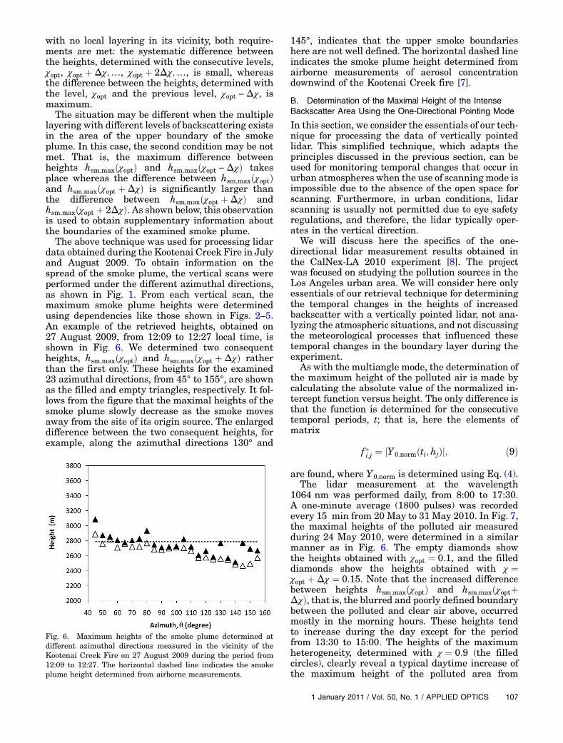
The above technique was used for processing lidardata obtained during the Kootenai Creek Fire in Julyand August 2009. To obtain information on thespread of the smoke plume, the vertical scans wereperformed under the different azimuthal directions,as shown in Fig. 1. From each vertical scan, themaximum smoke plume heights were determinedusing dependencies like those shown in Figs. 2–5.An example of the retrieved heights, obtained on27 August 2009, from 12:09 to 12:27 local time, isshown in Fig. 6. We determined two consequentheights, hsm;maxðχoptÞ and hsm;maxðχopt þΔχÞ ratherthan the first only. These heights for the examined23 azimuthal directions, from 45° to 155°, are shownas the filled and empty triangles, respectively. It fol-lows from the figure that the maximal heights of thesmoke plume slowly decrease as the smoke movesaway from the site of its origin source. The enlargeddifference between the two consequent heights, forexample, along the azimuthal directions 130° and

145°, indicates that the upper smoke boundarieshere are not well defined. The horizontal dashed lineindicates the smoke plume height determined fromairborne measurements of aerosol concentrationdownwind of the Kootenai Creek fire [7].

B. Determination of the Maximal Height of the IntenseBackscatter Area Using the One-Directional Pointing Mode

In this section, we consider the essentials of our tech-nique for processing the data of vertically pointedlidar. This simplified technique, which adapts theprinciples discussed in the previous section, can beused for monitoring temporal changes that occur inurban atmospheres when the use of scanningmode isimpossible due to the absence of the open space forscanning. Furthermore, in urban conditions, lidarscanning is usually not permitted due to eye safetyregulations, and therefore, the lidar typically oper-ates in the vertical direction.

We will discuss here the specifics of the one-directional lidar measurement results obtained inthe CalNex-LA 2010 experiment [8]. The projectwas focused on studying the pollution sources in theLos Angeles urban area. We will consider here onlyessentials of our retrieval technique for determiningthe temporal changes in the heights of increasedbackscatter with a vertically pointed lidar, not ana-lyzing the atmospheric situations, and not discussingthe meteorological processes that influenced thesetemporal changes in the boundary layer during theexperiment.

As with the multiangle mode, the determination ofthe maximum height of the polluted air is made bycalculating the absolute value of the normalized in-tercept function versus height. The only difference isthat the function is determined for the consecutivetemporal periods, t; that is, here the elements ofmatrix

f �i;j ¼ jY0;normðti;hjÞj; ð9Þ

are found, where Y0;norm is determined using Eq. (4).The lidar measurement at the wavelength

1064 nm was performed daily, from 8:00 to 17:30.A one-minute average (1800 pulses) was recordedevery 15 min from 20 May to 31 May 2010. In Fig. 7,the maximal heights of the polluted air measuredduring 24 May 2010, were determined in a similarmanner as in Fig. 6. The empty diamonds showthe heights obtained with χopt ¼ 0:1, and the filleddiamonds show the heights obtained with χ ¼χopt þΔχ ¼ 0:15. Note that the increased differencebetween heights hsm;maxðχoptÞ and hsm;maxðχoptþΔχÞ, that is, the blurred and poorly defined boundarybetween the polluted and clear air above, occurredmostly in the morning hours. These heights tendto increase during the day except for the periodfrom 13:30 to 15:00. The heights of the maximumheterogeneity, determined with χ ¼ 0:9 (the filledcircles), clearly reveal a typical daytime increase ofthe maximum height of the polluted area from

Fig. 6. Maximum heights of the smoke plume determined atdifferent azimuthal directions measured in the vicinity of theKootenai Creek Fire on 27 August 2009 during the period from12:09 to 12:27. The horizontal dashed line indicates the smokeplume height determined from airborne measurements.

1 January 2011 / Vol. 50, No. 1 / APPLIED OPTICS 107

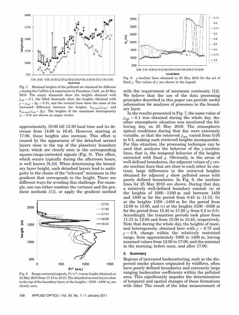
approximately, 10:00 till 13:30 local time and its de-crease from 14:00 to 16:45. However, starting at17:00, these heights also increase. This effect iscaused by the appearance of the detached aerosollayers close to the top of the planetary boundarylayer, which are clearly seen in the correspondingsquare-range-corrected signals (Fig. 8). This effect,which occurs typically during the afternoon hours,is well known [9,10]. When determining the bound-ary layer height, such detached layers lead to ambi-guity in the choice of the “relevant” minimum in thegradient that corresponds to the height. There aredifferent ways for avoiding this challenge. For exam-ple, one can either combine the variance and the gra-dient methods [11], or apply the gradient method

with the requirement of minimum continuity [12].We believe that the use of the data processingprinciples described in this paper can provide usefulinformation for analyses of processes in the bound-ary layer.

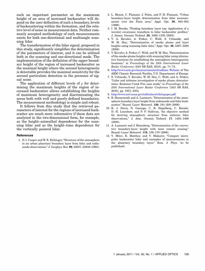
In the results presented in Fig. 7, the same value ofχopt ¼ 0:1 was obtained during the whole day. An-other atmospheric situation was monitored the fol-lowing day, on 25 May 2010. The atmosphericoptical conditions during that day were extremelyvariable, so that the retrieved χopt varied from 0.05to 0.5, making such retrieved heights incomparable.For this situation, the processing technique can beused that analyzes the behavior of the χ-isocliniclines, that is, the temporal behavior of the heightsextracted with fixed χ. Obviously, in the areas ofwell-defined boundaries, the adjacent values of χ cre-ate isoclinic lines that are close to each other. In con-trast, large differences in the retrieved heightsobtained for adjacent χ show polluted areas withpoorly defined boundaries. In Fig. 9, the isocliniclines for 25 May 2010 are shown. During that day,a relatively well-defined boundary existed: (a) atthe heights of 1000 –1100 m and between 1450and 1800 m for the period from 8:45 to 11:15, (b)at the heights 1350 –1450 m for the period from12:00 to 15:00, and (c) at the heights 3100 –3500 mfor the period from 15:45 to 17:30 (χ from 0.2 to 0.5).Accordingly, the transition periods took place from11:15 to 12:00 and from 15:00 to 15:45, respectively.Note that during the whole day, the heights of maxi-mal heterogeneity, obtained here with χ ¼ 0:75 andχ ¼ 0:9, change within the relatively restrictedrange, from approximately 1000 to 1400 m, havingmaximal values from 12:00 to 17:00, and theminimalin the morning, before noon, and after 17:00.

3. Summary

Regions of increased backscattering, such as the dis-persed smoke plumes originated by wildfires, oftenhave poorly defined boundaries and extremely largeranging backscatter coefficients within the pollutedarea. This significantly impedes the determinationof temporal and spatial changes of these formationswith lidar. The result of the lidar measurement of

Fig. 7. Maximal heights of the polluted air obtained for differentχ during the CalNex-LA experiment in Pasadena, Calif., on 24May2010. The empty diamonds show the heights obtained withχopt ¼ 0:1, the filled diamonds show the heights obtained withχ ¼ χopt þΔχ ¼ 0:15, and the vertical lines show the cases of theincreased difference between the heights, hsm;maxðχoptÞ andhsm;maxðχopt þΔχÞ. The heights of the maximum heterogeneity(χ ¼ 0:9) are shown as empty circles.

Fig. 8. Range-corrected signals, PðrÞr2, versus height obtained on24May 2010 from 17:15 to 18:15. The detached aerosol layers closeto the top of the boundary layer, at the heights ∼1550 –1850 m, areclearly seen.

Fig. 9. χ-isoclinic lines obtained on 25 May 2010 for the set offixed χ. The values of χ are shown in the legend.

108 APPLIED OPTICS / Vol. 50, No. 1 / 1 January 2011

such an important parameter as the maximumheight of an area of increased backscatter will de-pend on the user definition of such a boundary, levelsof backscattering within the formation, and the rela-tive level of noise inmeasurement data. Neither com-monly accepted methodology of such measurementsexists for both one-directional and multiangle scan-ning lidar.

The transformation of the lidar signal, proposed inthis study, significantly simplifies the determinationof the parameters of interest, and it can be utilizedboth in the scanning and one-directional mode. Theimplementation of the definition of the upper bound-ary height of the region of increased backscatter asthe maximal height where the aerosol heterogeneityis detectable provides the maximal sensitivity for theaerosol particulate detection in the presence of sig-nal noise.

The application of different levels of χ for deter-mining the maximum heights of the region of in-creased backscatter allows establishing the heightsof maximum heterogeneity and discriminating theareas both with well and poorly defined boundaries.The measurement methodology is simple and robust.

It follows from this study that the retrieved pa-rameters of interest for the regions of increased back-scatter are much more informative if these data areanalyzed in the two-dimensional form, for example,as the height–azimuthal dependence for the scan-ning lidar and as the height–time dependence forthe vertically pointed lidar.

References1. D. I. Cooper andW. E. Eichinger, “Structure of the atmosphere

in an urban planetary boundary layer from lidar and radio-sonde observations,” J. Geophys. Res. 99, 22937–22948 (1994).

2. L. Menut, C. Flamant, J. Pelon, and P. H. Flamant, “Urbanboundary-layer height determination from lidar measure-ments over the Paris area,” Appl. Opt. 38, 945–954(1999).

3. I. M. Brooks, “Finding boundary layer top: Application of awavelet covariance transform to lidar backscatter profiles,”J. Atmos. Oceanic Technol. 20, 1092–1105 (2003).

4. V. A. Kovalev, A. Petkov, C. Wold, S. Urbanski, andW. M. Hao, “Determination of smoke plume and layerheights using scanning lidar data,” Appl. Opt. 48, 5287–5294(2009).

5. V. Kovalev, A. Petkov, C. Wold, andW. M. Hao, “Determinationof the smoke-plume heights with scanning lidar using alterna-tive functions for establishing the atmospheric heterogeneitylocations,” in Proceedings of the 25th International LaserRadar Conference (IAO SB RAS, 2010), pp. 71–74.

6. http://www.arm.gov/measurements/cloudbase Website of TheARM Climate Research Facility, U.S. Department of Energy.

7. S. Urbanski, V. Kovalev, W. M. Hao, C. Wold, and A. Petkov,“Lidar and airborne investigation of smoke plume character-istics: Kootenai Creek Fire case study,” in Proceedings of the25th International Laser Radar Conference (IAO SB RAS,2010), pp. 1051–1054.

8. http://www.esrl.noaa.gov/csd/calnex/whitepaper.pdf.9. B. Hennemuth and A. Lammert, “Determination of the atmo-

spheric boundary layer height from radiosonde and lidar back-scatter,” Bound.-Layer Meteorol. 120, 181–200 (2006).

10. K. J. Davis, N. Gamage, C. R. Hagelberg, C. Kiemle,D. H. Lenschow, and P. P. Sullivan, “An objective methodfor deriving atmospheric structure from airborne lidarobservations,” J. Atm. Oceanic Technol. 17, 1455–1468(2000).

11. A. Lammert and J. Bösenberg, “Determination of the convec-tive boundary-layer height with laser remote sensing,”Bound.-Layer Meteorol. 119, 159–170 (2006).

12. V. Mitev, R. Matthey, and V. Makarov, “Compact micro-pulse backscatter lidar and examples of measurements inthe planetary boundary layer,” Rom. J. Phys. (to bepublished).

1 January 2011 / Vol. 50, No. 1 / APPLIED OPTICS 109