levy copulas: review of recent results´ · levy copulas: review of recent results´ peter tankov...

Levy copulas: review of recent results

Peter Tankov

Abstract We review and extend the now considerable literature on Levy copulas.First, we focus on Monte Carlo methods and present a new robust algorithm forthe simulation of multidimensional Levy processes with dependence given by aLevy copula. Next, we review statistical estimation techniques in a parametric and anon-parametric setting. Finally, we discuss the interplaybetween Levy copulas andmultivariate regular variation and briefly review the applications of Levy copulas inrisk management. In particular, we provide a new easy-to-use sufficient conditionfor multivariate regular variation of Levy measures in terms of their Levy copulas.

Key Words: Levy processes, Levy copulas, Monte Carlo simulation, statistical es-timation, risk management, regular variation

1 Introduction

Introduced in [13, 31, 42], the concept of Levy copula allows to characterize in atime-independent fashion the dependence structure of the pure jump part of a Levyprocess. During the past ten years, several authors have proposed extensions of Levycopulas, developed simulation and estimation techniques for these and related ob-jects, and studied the applications of these tools to financial risk management. In thispaper we review the early developments and the subsequent literature on Levy cop-ulas, present new simulation algorithms for Levy processes with dependence givenby a Levy copula, discuss the link between Levy copulas and multivariate regularvariation and mention some risk management applications. The aim is to provide asummary of available tools and an entry point to the now considerable literature on

Peter TankovLaboratoire de Probabilites et Modeles Aleatoires, Universite Paris Diderot, Paris, France and In-ternational Laboratory of Quantitative Finance, NationalResearch University Higher School ofEconomics, Moscow, Russia., e-mail: [email protected]

1

2 Peter Tankov

Levy copulas and more generally dependence models for multidimensional Levyprocesses. We focus on practical aspects such as statistical estimation and MonteCarlo simulation rather than theoretical properties of Levy copulas.

This chapter is structured as follows. In Section 2 we recallthe main definitionsand results from the theory of Levy copulas and review some alternative construc-tions and dependence models proposed in the literature. Section 3 presents newalgorithms for simulating Levy processes with a given Levy copula, via a series rep-resentation. Section 4 reviews the statistical proceduresproposed in the literature forestimating Levy copulas in the parametric or non-parametric setting. InSection 5we discuss the interplay between these objects and multivariate regular variation. Inparticular, we present a new easy-to-use sufficient condition for multivariate regularvariation of Levy measures in terms of their Levy copulas. In Section 6 we reviewthe applications of Levy copulas in risk management. Section 7 concludes the paperand discusses some directions for further research.

Remarks on notation In this chapter, the components of a vector are denoted bythe same letter with superscripts:X = (X1, . . . ,Xn). The scalar product of two vec-tors is written with angle brackets:〈X,Y〉 = ∑n

i=1XiYi , and the Euclidean norm ofthe vectorX is denoted by|X|. The extended real line is denoted byR := (−∞,∞].

2 A primer on L evy copulas

This section contains a brief review of the theory of Levy copulas as exposed in[13, 31, 42]. We invite the readers to consult these references for additional details.

Recall that a Levy process is a stochastic process with stationary and independentincrements, which is continuous in probability. The law of aLevy process(Xt)t≥0 iscompletely determined by the law ofXt at any given timet > 0. The characteristicfunction of this law is given explicitly by the Levy-Khintchine formula:

E[ei〈u,Xt 〉] = etψ(u), u∈ Rn,

ψ(u) =−〈Au,u〉2

+ i〈γ ,u〉+∫

Rn(ei〈u,x〉−1− i〈u,x〉1|x|≤1)ν(dx),

whereγ ∈ Rn, A is a positive semi-definiten×n matrix andν is a positive measure

onRn with ν({0})= 0 such that∫Rn(|x|2∧1)ν(dx)<∞. The triple(A,ν ,γ) is called

thecharacteristic tripleof the Levy processX.The Levy-Ito decomposition in turn gives a representation of the paths of X in

terms of a Brownian motion and a Poisson random measure:

Xt = γt +Bt +∫ t

0

∫

|x|≤1xJ(ds×dx)+

∫ t

0

∫

|x|>1xJ(ds×dx), (1)

whereB is a Brownian motion (centered Gaussian process with independent incre-ments) with covariance matrixA at timet = 1, J is a Poisson random measure with

Levy copulas: review of recent results 3

intensity measuredt×ν(dx) andJ is the compensated version ofJ. (Bt)t≥0 is thusthe continuous martingale part of the processX, and the remaining terms

γt +∫ t

0

∫

|x|≤1xJ(ds×dx)+

∫ t

0

∫

|x|>1xJ(ds×dx)

may be called the pure jump part ofX. Sinceγ corresponds to a deterministic shiftof every component, the law of the pure jump part of a Levy process is determinedessentially by the Levy measureν .

Levy copulas provide a representation of the Levy measure of a multidimensionalLevy process, which allows to specify separately the Levy measures of the compo-nents and the information about the dependence between the components1. Simi-larly to copulas for probability measures, this gives a flexible approach for buildingmultidimensional dynamic models based on Levy processes.

The main ideas of Levy copulas are simpler to explain in the context of Levymeasures on[0,∞)n, which correspond to Levy processes with only positive jumpsin every component. Formally, the definitions of Levy copula, tail integrals etc. aredifferent for Levy measures on[0,∞)n and on the full space, and we shall speak ofLevy copulas on[0,∞]n and of Levy copulas on(−∞,∞]n, respectively. However,when there is no ambiguity, the explicit mention of the domain will be dropped.Moreover, by comparing the two definitions below it is easy tosee that from a Levycopula on[0,∞]n one can always construct a Levy copula on(−∞,∞]n by setting itto zero outside its original domain.

Levy copulas on[0,∞]n Similarly to probability measures, which can be repre-sented through their distribution functions, Levy measures can be represented bytail integrals.

Definition 1 (Tail integral). Let ν be a Levy measure on[0,∞)n. The tail integralU of ν is a function[0,∞)n → [0,∞] such that

1. U(0, . . . ,0) = ∞.2. For(x1, . . . ,xn) ∈ [0,∞)n\{0},

U(x1, . . . ,xn) = ν([x1,∞)×·· ·× [xn,∞)).

The i-th one-dimensional marginal tail integralUi of aRn-valued Levy process

X = (X1, . . . ,Xn) is the tail integral of the processXi and can be computed as

Ui(z) = (U(x1, . . . ,xn)|xi = z;x j = 0 for j 6= i), z≥ 0.

We recall that a functionF : DomF ⊆ Rn → R is calledn-increasing if for all

a∈ DomF andb∈ DomF with ai ≤ bi for all i we have

VF((a,b]) := ∑c∈DomF :ci=ai or bi ,i=1...n

sgn(c)F(c)≥ 0,

1 By “dependence” we mean the information on the law of a random vector which remains to bedetermined once the marginal laws of its components have been specified.

4 Peter Tankov

sgn(c) =

{1, if ck = ak for an even number of indices,

−1, if ck = ak for an odd number of indices.

Definition 2 (Levy copula). A function F : [0,∞]n → [0,∞] is a Levy copulaon[0,∞]n if

1. F(u1, . . . ,un)< ∞ for (u1, . . . ,un) 6= (∞, . . . ,∞),2. F(u1, . . . ,un) = 0 wheneverui = 0 for at least onei ∈ {1, . . . ,n},3. F is n-increasing,4. Fi(u) = u for any i ∈ {1, . . . ,n}, u∈ [0,∞], where

Fi(u) = (F(v1, . . . ,vn)|vi = u;v j = 0 for j 6= i).

The following theorem gives a representation of the tail integral of a Levy mea-sure (and thus of the Levy measure itself) in terms of its marginal tail integrals anda Levy copula. It may be calledSklar’s theoremfor Levy copulas on[0,∞]n.

Theorem 1.Let ν be a Levy measure on[0,∞)n with tail integral U and marginalLevy measuresν1, . . . ,νn. Then there exists a Levy copula F on[0,∞]n such that

U(x1, . . . ,xn) = F(U1(x1), . . . ,Un(xn)), (x1, . . . ,xn) ∈ [0,∞)n, (2)

where U1, . . . ,Un are tail integrals ofν1, . . . ,νn. This Levy copula is unique on∏n

i=1RanUi .Conversely, if F is a Levy copula on[0,∞]n andν1, . . . ,νn are Levy measures on

[0,∞) with tail integrals U1, . . . ,Un then (2) defines a tail integral of a Levy measureon [0,∞)n with marginal Levy measuresν1, . . . ,νn.

A basic example of a one-parameter family of Levy copulas on[0,∞]n is theClayton family, given by

Fθ (u1, . . . ,un) = (u−θ1 + · · ·+u−θ

n )−1/θ , θ > 0. (3)

This family has as limiting cases the independence Levy copula (whenθ → 0)

F⊥(u1, . . . ,un) =n

∑i=1

ui ∏j 6=i

1{∞}(u j)

and the complete dependence Levy copula (whenθ → ∞)

F‖(u1, . . . ,un) = min(u1, . . . ,un).

Since Levy copulas are closely related to distribution copulas, many of the clas-sical copula constructions can be modified to build Levy copulas. This allows todefineArchimedean Levy copulas(see Propositions 5.6 and 5.7 in [13] for the caseof Levy copulas on[0,∞]n). Another example is the vine construction of Levy cop-ulas [26], where a Levy copula on[0,∞]n is constructed fromn(n−1)/2 bivariatedependence functions (n−1 Levy copulas and(n−2)(n−1)/2 distributional cop-ulas).


Levy copulas on(−∞,∞]n For Levy measures on the full spaceRn, the definitionof a Levy copula is more complex because the singularity of the Levy measure islocated in the interior of the domain and not at the boundary.The tail integral isdefined so as to avoid this singularity.

Definition 3. Let ν be a Levy measure onRn. Thetail integral of ν is the functionU : (R\{0})n → R defined by

U(x1, . . . ,xn) := ν

(n

∏j=1

I (x j)

)d

∏i=1

sgn(xi), (4)

where

I (x) :=

{[x,∞), x≥ 0,

(−∞,x), x< 0.

In the above definition, the signs and the intervals are chosen in such way that thetail integral becomes a left-continuousn-increasing function on each orthant.

Given a set of indicesI ⊂ {1, . . . ,n}, the I -marginal tail integralU I of the LevyprocessX = (X1, . . . ,Xn) is the tail integral of the process(Xi)i∈I containing thecomponents ofX with indices inI . The one-dimensional tail integrals are, as before,denoted byUi ≡U{i}. Given anRn-valued Levy processX, its marginal tail integrals{U I : I ⊂ {1, . . . ,n} nonempty} are, of course, uniquely determined by its Levymeasureν .

The tail integral for a Levy measure onRn, as well as the marginal tail integrals,are only defined for nonzero arguments. This leads to a symmetric definition, whichresults in a simple statement for Sklar’s theorem below. On the other hand, thismeans that when the Levy measure is not absolutely continuous, it is not uniquelydetermined by its tail integral. However, it is always uniquely determined by the set{U I , I ⊆ {1, . . . ,n}, I 6= /0} containing its tail integral as well as all its marginal tailintegrals.

Definition 4. A functionF : (−∞,∞]n → (−∞,∞] is aLevy copulaon (−∞,∞]n if

1. F(u1, . . . ,un)< ∞ for (u1, . . . ,un) 6= (∞, . . . ,∞),2. F(u1, . . . ,un) = 0 if ui = 0 for at least onei ∈ {1, . . . ,n},3. F is n-increasing,4. Fi(u) = u for any i ∈ {1, . . . ,n}, u∈ (−∞,∞], whereFi is defined below.

The margins of a Levy copula on(−∞,∞]n are defined by

F I ((xi)i∈I ) := limc→∞ ∑

(x j ) j∈Ic∈{−c,∞}|Ic|F(x1, . . . ,xn) ∏

j∈Icsgnx j (5)

with the conventionFi = F{i} for one-dimensional margins.The following theorem is the analogue of Sklar’s theorem forLevy copulas on

(−∞,∞]n.

6 Peter Tankov

Theorem 2.Letν be a Levy measure onRn. Then there exists a Levy copula F suchthat the tail integrals ofν satisfy:

U I ((xi)i∈I ) = F I ((Ui(xi))i∈I ) (6)

for any non-empty I⊆ {1, . . . ,n} and any(xi)i∈I ∈ (R\{0})I . The Levy copula F isunique on∏n

i=1RanUi .Conversely, if F is a n-dimensional Levy copula andν1, . . . ,νn are Levy measures

onR with tail integrals Ui , i = 1, . . . ,n then there exists a unique Levy measure onR

n with one-dimensional marginal tail integrals U1, . . . ,Un and whose marginal tailintegrals satisfy (6) for any non-empty I⊆ {1, . . . ,n} and any(xi)i∈I ∈ (R\{0})I .

A basic example of a Levy copula on(−∞,∞]n is the two-parameter Claytonfamily which has the form

F(u1, . . . ,un) = 22−n

(d

∑i=1

|ui |−θ

)−1/θ

(η1u1...un≥0− (1−η)1u1...un<0), (7)

for θ > 0 andη ∈ [0,1]. Here the parameterη determines the dependence of thesign of the jumps: for example, whenn= 2 andη = 1, the two components alwaysjump in the same direction. The parameterθ , as before, determines the dependenceof the amplitude of the jumps. Whenη = 1 andθ → 0, the Clayton Levy copulaconverges to the independence Levy copula

F⊥(u1, . . . ,un) =n

∑i=1

ui ∏j 6=i

1{∞}(u j),

and whenη = 1 andθ → ∞, one recovers the complete dependence Levy copula

F⊥(u1, . . . ,un) = min(|u1|, . . . , |un|)1K(u1, . . . ,un)n

∏i=1

sgnui ,

whereK = {u∈ Rn : sgnu1 = · · ·= sgnun}.

Other families of Levy copulas on(−∞,∞]n may be obtained using the ArchimedeanLevy copula construction (Theorem 5.1 in [31]) or, when a precise description ofdependence in each orthant is needed, from 2n Levy copulas on[0,∞]n (Theorem5.3 in [31]).

Alternative marginal transformations WhenF is a Levy copula on[0,∞]n, themapping

χF((0,b1]×·· ·× (0,bn]) := F(b1, . . . ,bn), 0≤ b1, . . . ,bn ≤ ∞

can be extended to a unique positive measureχF on the Borel sets of[0,∞]n, whosemargins (projections on the coordinate axes) are uniform (standard Lebesgue) mea-sures on[0,∞), and which has no atom at{∞, . . . ,∞}. Similarly, a Levy copulaFon (−∞,∞]n can be associated to a positive measureχF whose margins are uniform


measures on(−∞,∞), and which satisfies

χF((a1,b1]×·· ·× (an,bn]) =VF((a,b]), −∞ < ai ≤ bi ≤ ∞, i = 1, . . . ,n. (8)

The transformation to uniform margins offers a direct analogy with the distributionalcopulas, but other marginal transformations may be more convenient in specificcontexts.

In particular, several authors [2, 18, 33] have considered the transformation to1-stable margins. Following [2], introduce the “inversionmap”

Q : [0,∞]n → [0,∞]n, (x1, . . . ,xn) 7→ (x−11 , . . . ,x−1

n ),

where 1/0 has to be interpreted as∞ and 1/∞ as 0. For a Levy copulaF on [0,∞]n,we define the measureνF as the image of the measureχF defined above under themappingQ, that is,

νF(B) = χF(Q−1(B)) ∀B Borel set in[0,∞]n.

Then,νF is a Levy measure on[0,∞)n with marginal tail integralsUk(x) = x−1,that is,νF has 1-stable margins. It is clear that the dependence structure of a Levymeasure with Levy copulaF can be alternatively characterized in terms of the LevymeasureνF . This construction has been extended to Levy measures onRn [18] (inthis reference, the Levy measureνF has been calledPareto Levy measurein and itstail integral has been calledPareto Levy copula).

A brief review of alternative dependence modelsLevy copulas offer a very flex-ible approach to build multidimensional Levy processes with a precise control overthe dependence of joint jumps and joint extremes. However, this degree of preci-sion is not needed for all applications and comes at the priceof reduced analyticaltractability. For this reason, several authors have proposed alternative approaches togenerate dependency among Levy processes, which may be less flexible, but lead tosimpler models. Among the possible alternative approachesone can mention

• Brownian subordination (time change) with a one-dimensional subordinator [15,35, 38] or a multi-dimensional subordinator [3, 16].

• Factor models based on linear combinations of independent Poisson shocks [34]or more generally independent Levy processes [32, 36, 37].

Levy copulas allow to construct a multidimensional Levy process with givenmarginals and given dependence structure. The same question has been addressedfor other classes of stochastic processes such as Markov processes [7] and semi-martingales [46]. We refer the reader to [6] for a comprehensive review of copula-related concepts for these processes.

8 Peter Tankov

3 Monte Carlo simulation of Levy processes with a specifiedLevy copula

In models based on Levy copulas, explicit computations are rarely possible (forinstance, the characteristic function of the Levy process is usually not known inexplicit form), and to compute quantities such as option prices, one has to resortto numerical methods which can be either deterministic (partial integro-differentialequations) or stochastic (Monte Carlo). Deterministic numerical methods for PIDEsarising in Levy copula models have been developed in [24, 27, 39]. In thissec-tion, we propose a new algorithm for simulating multidimensional Levy processesdefined through a Levy copula, which can be used for Monte Carlo simulation.

Let F be a Levy copula such that for everyI ⊆ {1, . . . ,n} nonempty,

lim(xi)i∈I→∞

F(x1, . . . ,xn) = F(x1, . . . ,xn)|(xi)i∈I=∞. (9)

As mentioned above, this Levy copula is associated to a positive measureχF on Rn

with Lebesgue margins, and condition (9) guarantees that this measure is supportedby R

n.The following technical lemma, whose proof can be found in the preprint [43],

establishes the relation betweenχF and the Levy measures of processes havingF astheir Levy copula. For a one-dimensional tail integralU , the (generalized) inversetail integralU (−1) is defined by

U (−1)(u) :=

{sup{x> 0 :U(x)≥ u}∨0, u≥ 0sup{x< 0 :U(x)≥ u}, u< 0.

(10)

Lemma 1. Let ν be a Levy measure onRn with marginal tail integrals Ui , i =1, . . . ,n, and Levy copula F satisfying the condition(9), let χF be defined by(8)and let

f : (u1, . . . ,un) 7→ (U (−1)1 (u1), . . . ,U

(−1)n (un)).

Thenν is the image measure ofχF by f .

In Theorems 3 and 4 below, to simulate the jumps of a multidimensional Levyprocess (more precisely, of the corresponding Poisson random measure), we willchoose one component of the Levy process, simulate its jumps, and then simulatethe jumps in the other components conditionally on the jumpsin the chosen one. Wetherefore proceed by analyzing the conditional distributions ofχF . To fix the ideas,we suppose that we have chosen the first component of the Levy process, but theconditional distribution with respect to any other component is obtained in the sameway.

By Theorem 2.28 in [1], there exists a family, indexed byξ ∈ R, of positiveRadon measuresK1(ξ ,dx2 · · ·dxn) onR

n−1, such that

ξ 7→ K1(ξ ,dx2 · · ·dxn)


is Borel measurable and

χF(dx1 . . .dxn) = dx1×K1(x1,dx2 · · ·dxn). (11)

In addition,K1(ξ ,Rn−1) = 1 almost everywhere, that is,K1(ξ , ·) is, almost every-where, a probability distribution. In the sequel we will call {K1(ξ , ·)}ξ∈R the familyof conditional probability distributions with respect to the first component associ-ated with the Levy copulaF . Similarly, the conditional distributions with respect toother components will be denoted byK2, . . . ,Kn.

Let Fξ1 be the distribution function of the measureK1(ξ , ·):

Fξ1 (x2, . . . ,xn) := K1(ξ ,(−∞,x2]×·· ·× (−∞,xn]). (12)

The following lemma, whose proof can also be found in [43], shows that it can becomputed in a simple manner from the Levy copulaF . We recall that the law of arandom variable is completely determined by the values of its distribution functionat the continuity points of the latter.

Lemma 2. Let F be a Levy copula satisfying(9), and Fξ1 be the corresponding

conditional distribution function, defined by(12). Then, there exists a set N⊂ R of

zero Lebesgue measure such that for every fixedξ ∈ R \N, Fξ1 (·) is a probability

distribution function, satisfying

Fξ1 (x2, . . . ,xn)

= sgn(ξ )∂

∂ξVF((ξ ∧0,ξ ∨0]× (−∞,x2]×·· ·× (−∞,xn]) (13)

in every point(x2, . . . ,xn), where Fξ1 is continuous.

In the following two theorems we show how Levy copulas may be used to sim-ulate multidimensional Levy processes with a specified dependence structure. Ourresults can be seen as an extension to Levy processes, represented by Levy copulas,of the series representation results, developed by Rosinski and others (see [41] andreferences therein). The first result concerns the simpler case when the Levy processhas finite variation on compacts.

Theorem 3. (Simulation of multidimensional Levy processes, finite variationcase)Let ν be a Levy measure onRn, satisfying

∫(|x| ∧1)ν(dx) < ∞, with marginal tail

integrals Ui , i = 1, . . . ,n and Levy copula F(x1, . . . ,xn), such that(9) is satisfied,and let K1, . . . ,Kn be the corresponding conditional probability distributions.

Fix a truncation levelτ. Let (Vk) and(Wik) for 1≤ i ≤ n and k≥ 1 be indepen-

dent sequences of independent random variables, uniformlydistributed on[0,1].Introduce n2 random sequences(Γ i j

k )1≤i, j≤nk≥1 , independent from(Vi) and (Wi) such

that

10 Peter Tankov

• For i = 1, . . . ,n,∑∞k=1 δ{Γ ii

k } are independent Poisson random measures onR withLebesgue intensity measures.

• Conditionally onΓ iik , the random vector(Γ i1

k , . . . ,Γ i,i−1k ,Γ i,i+1

k , . . . ,Γ ink ) is inde-

pendent fromΓ pql with 1 ≤ p,q ≤ n and l 6= k and fromΓ pq

k with p 6= i and1≤ q≤ n and is distributed onRn−1 with law Ki(Γ ii

k ,dx1 · · ·dxn−1).

For each k≥ 1 and each i= 1, . . . ,n, let nik = #{ j = 1, . . . ,n : |Γ i j

k | ≤ τ}. Then theprocess(Zτ

t )0≤t≤1 with components

Zτ , jt =

∞

∑k=1

n

∑i=1

U (−1)j (Γ i j

k )1nikW

ik≤11|Γ ii

k |≤τ1[0,t](Vk), j = 1, . . . ,n, (14)

is a Levy process on[0,1] with characteristic function

E[ei〈u,Zτ

t 〉]= exp

(t∫

Rn\Sτ(ei〈u,z〉−1)ν(dz)

), (15)

where

Sτ = (U (−1)1 (−τ),U (−1)

1 (τ))×·· ·× (U (−1)n (−τ),U (−1)

n (τ)). (16)

Moreover, there exists a Levy process(Zt)0≤t≤1 with characteristic function

E[ei〈u,Zt 〉

]= exp

(t∫

Rn(ei〈u,z〉−1)ν(dz)

)(17)

such that

E[ sup0≤t≤1

|Zτt −Zt |]≤

n

∑i=1

∫ U(−1)i (τ)

U(−1)i (−τ)

|z|νi(dz), (18)

whereνi is the i-th margin of the Levy measure.

Remark 1.Since the Levy measure satisfies∫(|x|∧1)ν(dx)< ∞, the error (18) con-

verges to 0 asτ → +∞; in addition, the upper bound on the error does not dependon the Levy copulaF .

Remark 2.For the numerical computation of the sum in (14), we need to simulateonly the variablesΓ ii

k for which |Γ iik | ≤ τ. The number of such variables is a.s.

finite and followis the Poisson distribution with intensity2τ. They can therefore besimulated with the following two-step algorithm:

• Simulate a Poisson random variableNi with intensity 2τ.• SimulateNi independent random variablesU1, . . . ,UNi with uniform distribution

on [−τ ,τ ] and letΓ iik =Uk for k= 1, . . . ,Ni .

Remark 3.In [43] we proposed a simpler algorithm for simulating a Levy processwith a given Levy copula, where all the components were simulated conditionally


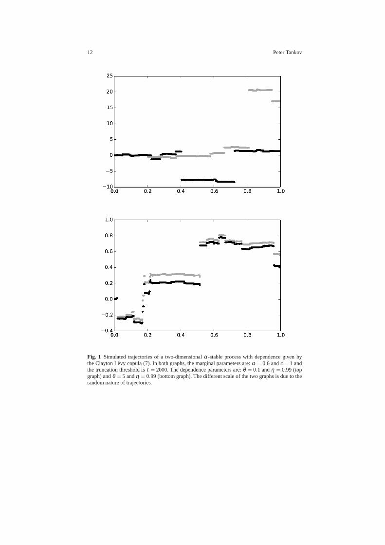
on the first one. As it turns out, this algorithm suffers from convergence problemswhen the components are weakly dependent. By contrast, the above algorithm treatsall components in a symmetric way, which leads to a uniform bound (18) ensuringfast convergence even in the case of weak dependence, at the price of performingadditional simulations and rejections. From Figure 1, one can see that even in thecase of very weak dependence, no single component appears todominate the otherone.

Example 1.Let d = 2 andF be the two-parameter Clayton Levy copula (7). Astraightforward computation yields:

Fξ1 (x) = Fξ

2 (x) := Fξ (x) =

(1−η)+

(1+

∣∣∣∣ξx

∣∣∣∣θ)−1−1/θ

(η −1x<0)

1ξ≥0

+

η +

(1+

∣∣∣∣ξx

∣∣∣∣θ)−1−1/θ

(1x≥0−η)

1ξ<0. (19)

This conditional distribution function can be inverted analytically:

F−1ξ (u) = B(ξ ,u)|ξ |

{C(ξ ,u)−

θθ+1 −1

}−1/θ

with B(ξ ,u) = sgn(u−1+η)1ξ≥0+sgn(u−η)1ξ<0

and C(ξ ,u) ={

u−1+ηη

1u≥1−η +1−η −u

1−η1u<1−η

}1ξ≥0

+

{u−η1−η

1u≥η +η −u

η1u<η

}1ξ<0.

Therefore, the sequences(Γ i, jk )1≤i, j≤2

k≥1 , introduced in Theorem 3, can be con-structed as follows:

• Simulate the variablesN1 andN2 and the sequences(Γ 11k )1≤k≤N1 and(Γ 22

k )1≤k≤N2

as described in Remark 2.• For all 1≤ k≤ N1, letΓ 12

k = F−1Γ 11

k(Y1

k ) and for all 1≤ k≤ N2 let Γ 21k = F−1

Γ 22k(Y2

k ),

where(Y1k )k≥0 and(Y2

k )k≥0 are independent sequences of independent randomvariables with uniform distribution on[0,1].

For the purpose of numerical illustration, we have simulated the trajectories ofa two-dimensionalα-stable process with marginal Levy densityν(x) = αc

|x|1+α for

both components and dependence given by the Clayton Levy copula (7) with weakdependence (Figure 1, left graph) and strong dependence (Figure 1, right graph). Weused the truncation parameterτ = 2000, which corresponds to keeping about 4000jumps in every component. For this value, the upper bound on the error (18) is equal

to 4cα1−α

(cτ) 1−α

α ≈ 0.037.

12 Peter Tankov

Fig. 1 Simulated trajectories of a two-dimensionalα-stable process with dependence given bythe Clayton Levy copula (7). In both graphs, the marginal parameters are:α = 0.6 andc= 1 andthe truncation threshold isτ = 2000. The dependence parameters are:θ = 0.1 andη = 0.99 (topgraph) andθ = 5 andη = 0.99 (bottom graph). The different scale of the two graphs is dueto therandom nature of trajectories.


Proof (of Theorem 3).First note that(Γ i jk ) are well defined since by Lemma 2,

Ki(ξ , ·) is a probability distribution for almost allξ . Let

Zτ ,i jt = ∑

k:|Γ iik |≤τ

U (−1)j (Γ i j

k )1nikW

ik≤11[0,t](Vk)

By Proposition 3.8 in [40],

Zτ ,i jt =

∫

[0,t]×RnU (−1)

j (x j)Mi(ds×dx1 · · ·dxn),

whereMi is a Poisson random measure on[0,1]×Rn with intensity measuredt×

ηi(x1, . . . ,xn)χF(dx1 · · ·dxn), and the functionηi is defined by

ηi(x1, . . . ,xn) =1|xi |≤τ

1+#{ j = 1, . . . ,n : j 6= i, |x j | ≤ τ} .

Therefore,

Zτ , jt =

n

∑i=1

Zτ ,i jt =

∫

[0,t]×RnU (−1)

j (x j)M(ds×dx1 · · ·dxn),

whereMi is a Poisson random measure on[0,1]×Rn with intensity measuredt×

η(x1, . . . ,xn)χF(dx1 · · ·dxn) with

η(x1, . . . ,xn) =n

∑i=1

ηi(x1, . . . ,xn) = 1−1|xi |>τ ,i=1,...,n.

By Lemma 1 and Proposition 3.7 in [40],

Zτ , jt =

∫

[0,t]×Rnx jNτ(ds×dx1 · · ·dxn) (20)

for a Poisson random measureNτ on [0,1]× Rn with intensity measureds×

ντ(dx1 · · ·dxn), where

ντ := (1−1Sτ (x1, . . . ,xn))ν(dx1 · · ·dxn). (21)

The Levy-Ito decomposition (1) then implies thatZτt is a Levy process on[0,1] with

characteristic function

E[ei〈u,Zτ

t 〉]= exp

(t∫

Rn(ei〈u,z〉−1)ντ(dz)

)= exp

(t∫

Rn\Sτ(ei〈u,z〉−1)ν(dz)

).

Now letRτ ∈ Rn be defined by

Rτ , jt =

∫

[0,t]×Rnx j Nτ(ds×dx1 . . .dxn);

14 Peter Tankov

whereNτ is a Poisson random measure on[0,1]×Rn with intensity measureds×

1Sτ (x1, . . . ,xn)ν(dx1 · · ·dxn), independent fromNτ . It is clear thatZ = Zτ +Rτ is aLevy process with characteristic function (17). Finally,

E[ sup0≤t≤1

|Zt −Zτt |]≤ E

[

∑0≤t≤1

|∆Rτt |]≤

n

∑i=1

E

[

∑0≤t≤1

|∆Rτ ,it |]

=n

∑i=1

∫

Rn|x|1Sτ ν(dx)≤

n

∑i=1

∫ U(−1)i (τ)

U(−1)i (−τ)

|z|νi(dz).

which proves the bound (18).

If the Levy process has paths of infinite variation on compact sets, it can no longerbe represented as the sum of its jumps and we have to introducea centering terminto the series (14).

Theorem 4. (Simulation of multidimensional Levy processes, infinite variationcase)Letν be a Levy measure onRn with marginal tail integrals Ui , i = 1, . . . ,n and Levycopula F(x1, . . . ,xn), such that the condition(9) is satisfied. Let(Vk)k≥1, (Wi

k)k≥1

for 1≤ i ≤ n and(Γ i jk )k≥1 for 1≤ i, j ≤ n be as in Theorem 3. Let

Ak(τ) =∫

Rn\Sτ1|x|≤1xkν(dx1 · · ·dxn), k= 1. . .n,

where Sτ is defined in(16). Then the process

(Zτt )0≤t≤1, where Zτ , j

t =∞

∑k=1

n

∑i=1

U (−1)j (Γ i j

k )1nikW

ik≤11|Γ ii

k |≤τ1[0,t](Vk)− tA j(τ),

for 1≤ j ≤ n is a Levy process on[0,1] with characteristic function

E

[ei〈u,Zτ

t 〉]= exp

(t∫

Rn\Sτ(ei〈u,x〉−1− i〈u,x〉)1|x|≤1ν(dx)

). (22)

Moreover, there exists a Levy process(Zt)0≤t≤1 with characteristic function

E

[ei〈u,Zt 〉

]= exp

(t∫

Rn(ei〈u,x〉−1− i〈u,x〉)1|x|≤1ν(dx)

)

such that

E

[sup

0≤t≤1(Zt −Zτ

t )2]≤ 4

n

∑i=1

∫ U−1i (τ)

U−1i (−τ)

z2νi(dz).

Proof. The proof is essentially the same as in Theorem 3. In this theorem, due tothe presence of the compensating termtA(τ), the processZτ is a martingale and theerror bound follows from Doob’s martingale inequality.


4 Statistical estimation techniques

Levy copulas give access to the distribution of sizes of simultaneous jumps of thedifferent components of a Levy process. Therefore, Levy copula-based models areeasy to estimate when jumps are observable. This is the case,for instance, in insur-ance models where jumps represent claims whose dates and amounts are known2.Esmaeli and Kluppelberg [21] use maximum likelihood for the statistical estimationof the parameters of a two-dimensional compound Poisson process with dependencegiven by a Levy copula, assuming that all jumps in both components are perfectlyobservable. The method is then applied to the Danish fire insurance data (see also[19, paragraph 6.5.2] for a discussion of this data in a one-dimensional setting).

In the case of infinite jump intensity it is clearly not realistic to assume thatall jumps are perfectly observable. For this reason, in the case of a bivariate sta-ble subordinator with dependence given by the Clayton Levy copula, Esmaeli andKl uppelberg [22] assume that one observes all simultaneous jumps whose value islarger than a certain small parameterε for both components. Once again, the exactknowledge of jump times and sizes allows to write down the maximum likelihoodestimator, which is shown to be consistent and asymptotically normal asε tends tozero and/or the observation horizon tends to infinity.

In Esmaeli and Kluppelberg [23], the authors consider a slightly different ob-servation scheme, assuming that jumps larger thanε in each single component arerecorded (this sampling scheme is also adopted in [26]). A two-step parameter es-timation scheme is developed, where one first estimates the parameters of the one-dimensional marginal Levy processes, and next those of the Levy copula. This re-duces the computational cost compared to full likelihood (simultaneous estimationof all parameters), at the price of a somewhat lower efficiency. The example of abivariate stable subordinator with Clayton dependence is worked out in detail. Thetwo-step estimator is shown to be consistent and asymptotically normal and the ef-ficiency loss as compared to the full likelihood estimator isshown to be quite small(the root mean square error increases by less than ten percentage points in mostcases).

In financial applications it is not always possible to assumethat all jumps ofsufficient size are perfectly observable: usually one only observes the Levy processat a discrete time grid. If the monitoring frequency is sufficiently high though, thejumps remain “almost” observable and the Levy copula can still be recovered.

Bucher and Vetter [11] develop a fully nonparametric approach for estimating thetail integrals and the Pareto Levy copula (see Section 2) in the context of bivariateLevy processes with only positive jumps. Their estimate for the bivariate tail integralbecomes

Un(x1,x2) =1kn

n

∑j=1

1{∆nj X(1)≥x1,∆n

j X(2)≥x2},

2 The underlying assumption in Levy insurance models is that dependence may only be presentamong simultaneous losses in different business lines. This is of course an over-simplification ofreality since in practice, losses resulting from the same event may become known at different times,introducing dependence between non-simultaneous jumps.

16 Peter Tankov

where∆ nj X

(i) ≥ x1 = X(i)j∆n

−X(i)( j−1)∆n

for i = 1,2, kn = n∆n, ∆n is the observationinterval andn is the sample size. The method of using the increments of the pro-cess larger than a given size as a proxy for its jumps is rathercommon in the highfrequency financial econometrics literature. The one-dimensional tail integrals areapproximated by

Ui,n(x) =1kn

n

∑j=1

1{∆nj X(i)≥x}, i = 1, . . . ,2,

and the estimator of the Pareto Levy copula is given, up to some technical adjust-ments, by

Γn(u1,u2) =Un

(U (−1)

n,1 (1/u1),U(−1)n,2 (1/u2)

).

These estimates for the tail integrals and the Pareto Levy copula are shown to con-verge at the rate1√

knasn→ ∞ provided that∆n → 0 (high frequency observation),

kn → ∞ (infinite time horizon) and in addition√

kn∆n → 0.We refer the reader to [11] for more details on the estimationprocedure as well

as for extensions to irregular and asynchronous sampling schemes. See also [9] foran alternative method of estimating the joint dependence ofjumps using the extremevalue theory. Another relevant reference is [25] where the so called jump tail depen-dence parameter (the analogue of the tail dependence index defined at the level ofthe Levy copula) is estimated from discrete observations of the Levy process.

5 Levy copulas and multivariate regular variation

Multivariate regular variation is a widely accepted framework for risk analysis in amultidimensional setting (see e.g., [20] for examples), which turns out to be wellsuited for Levy copula modeling.

For introduction to multivariate regular variation, see [4, 14, 30, 40]. Following[30], we let M0 denote the class of Borel measures onR

n, whose restriction toR

n \B0,r is finite for eachr > 0, whereB0,r is the ball of radiusr centered at theorigin. Further, letC0 be the class of real-valued bounded and continuous functionson R

n, vanishing in a neighborhood of zero. We say that a sequence of measures(µn)n≥1 ⊂ M0 converges inM0 to a measureµ ∈ M0 whenever

∫f (x)µn(dx)→

∫f (x)µ(dx), n→ ∞,

for eachf ∈ C0. This convergence is known as vague convergence of measuresandit is, of course, similar to weak convergence, the only difference being that the testfunctions must vanish in the neighborhood of zero.

A measureν ∈ M0 is said to be regularly varying if there exists a norming se-quence(cn)n≥1 of positive numbers withcn ↑ ∞ asn → ∞ and a nonzeroµ ∈ M0


such thatnν(cn ·) → µ in M0 asn → ∞. Then necessarily the limit measureµ ishomogeneous of some degreeα and we writeν ∈ RV(α,(cn),µ). A random vec-tor X ∈ R

n is said to be regularly varying if its probability distribution is regularlyvarying.

For infinitely divisible random vectors, multivariate regular variation is charac-terized in terms of the Levy measure: ifX is infinitely divisible with Levy measureνthenX ∈RV(α,(cn),µ) if and only if ν ∈RV(α,(cn),µ) [29]. Under this condition,the Levy process(Xt)0≤t≤1 with Levy measureν is regularly varying on the spaceD([0,1],Rd) of right-continuous functions with left limits [28]. The limiting mea-sure is concentrated on the trajectories of the formZ1t≤V with Z∈R

d andV ∈ [0,1],so that intuitively the extremal behavior of such a process is determined by one largejump.

The link between multivariate regular variation and Levy copulas is explored indetail in [18] using the closely related notion of Pareto Levy copulas (see Section2 above). Loosely speaking, if the Levy measures of the components are regularlyvarying with the same indexα and the Pareto Levy measure is multivariate regularlyvarying with index 1 then the Levy measureν is multivariate regularly varying withindexα (see Theorem 3.1 in [18] for a precise statement). Here, we shall summarizethe main ideas in terms of standard Levy copulas.

Definition 5. Let F be a Levy copula on(−∞,∞]n. We say thatF is regularlyvarying if there exists a Levy copulaG on (−∞,∞]n such that for any nonemptyI ⊆ {1, . . . ,n} and anyx∈ (R\{0})|I |,

nFI (n−1x)→ GI (x), n→ ∞. (23)

It is clear that in this case, the limiting Levy copulaG is homogeneous of order1. Examples of Levy copulas satisfying Assumption (23) include the independenceLevy copula, the complete dependence Levy copula, or the Clayton family.

For regularly varying Levy copulas, tail properties of the infinitely divisible ran-dom vector may be deduced from the corresponding propertiesof the Levy copula.For example, the following result gives a sufficient condition for a Levy measure(and thus for an infinitely divisible distribution) to be regularly varying.

Theorem 5.Letν be a Levy measure onRn with Levy copula F and one-dimensionalmarginal tail integrals U1, . . . ,Un. Assume that

• F is regularly varying with limiting Levy copula G;• There exist a sequence of positive numbers(cn)n≥1, a constantα ∈ (0,2) and

nonnegative numbers p+1 , . . . , p+n , p−1 , . . . , p

−n with p+i + p−i > 0 for at least one

i, such that for all i= 1, . . . ,n and all x> 0,

limn→∞

nUi(cnx) = p+i |x|−α and limn→∞

nUi(−cnx) =−p−i |x|−α .

Then,ν ∈ RV(α,(cn), ν), whereν is a Levy measure with Levy copula G whoseone-dimensional marginal tail integrals are given by

18 Peter Tankov

Ui(x) =

{p+i |x|−α , x> 0,

p−i |x|−α , x< 0.

Remark 4.Since the Levy copulaG is homogeneous of order 1, the limiting measureν is the Levy measure of anα-stable process (see [31, Theorem 4.8]).

Proof. First observe that sets of the form

{(y1, . . . ,yn) ∈ Rn : yi ∈ I (xi), i ∈ I}

for all I ⊆ {1, . . . ,n} nonempty and all(xi)i∈I ∈ (R \ {0})|I |, form a convergence-determining class for theM0-convergence of measures onRn. Second, due to conti-nuity ofGwith respect to each of its arguments and the continuity ofU1, the measureν does not charge the boundaries of such sets. Therefore, it remains to prove that forall I ⊆ {1, . . . ,n} nonempty and all(xi)i∈I ∈ (R\{0})|I |, theI -marginal tail integralof ν , denoted byU I , satisfies

nUI (cn(xi)i∈I )→ U I ((xi)i∈I ),

asn→ ∞, whereU I is theI -marginal tail integral ofν . By Sklar’s theorem, this isequivalent to

nFI ((Ui(cnxi))i∈I )→ GI ((Ui(xi))i∈I ),

which follows from our assumptions and from the continuity of the limiting LevycopulaG.

As an application of Theorem 5, we can compute the tail dependence coefficientsof an infinitely divisible random vector (see also [18] for a related discussion). Re-call that for a two-dimensional random vector(X,Y) with continuous marginal dis-tributionsFX andFY, the upper tail dependence coefficient is defined by

λU = limu→1−

P[Y > F−1Y (u)|X > F−1

X (u)]

and the lower tail dependence coefficient is defined by

λL = limu→0+

P[Y ≤ F−1Y (u)|X ≤ F−1

X (u)].

These coefficients depend only on the copula of(X,Y).

Proposition 1. Let (X1,X2) be an infinitely divisible random vector whose Levymeasureν satisfies the assumptions of Theorem 5, with Levy copula F and limit-ing Levy copula G, and the coefficients p+

1 , p−1 , p+2 and p−2 which are all strictlypositive. Then,

λU = limu→0+

u−1F(u,u) = G(1,1), λL = limu→0+

u−1F(−u,−u) = G(−1,−1).

Proof. Denote the distribution functions ofX1 andX2 by F1 andF2, respectively.By Theorem 5,ν ∈ RV(α,(cn), ν), and so(X1,X2) ∈ RV(α,(cn), ν). Under the as-


sumptions of Theorem 5, it is easy to show that asx→+∞,

F−12 (F1(x))∼ x

(p+1p+2

)−1/α

.

Therefore,

λU = limz→+∞

P[X2 > F−1

2 (F1(z)),X1 > z]

P[X1 > z]= lim

z→+∞

P

[X2 > z

(p+1p+2

)−1/α,X1 > z

]

P[X1 > z]

= limn→+∞

nP

[X2 > cn

(p+1p+2

)−1/α,X1 > cn

]

nP[X1 > cn]=

ν((1,∞)×

((p+1p+2

)−1/α,∞))

ν((1,∞)×R)

=

G

(U1(1),U2

((p+1p+2

)−1/α))

U1(1)= G(1,1)

by the homogeneity ofG. The coefficientλL can be computed along the same lines.

For example, for an infinitely divisible vector with regularly varying margins andClayton Levy copula (7), the tail dependence coefficients are given by

λU = λL = 2−1/θ η

6 Risk management applications

Levy copulas allow for a high degree of precision in modeling joint jump depen-dence, and as such are well suited for risk management problems where joint ex-treme moves in different assets play a major role. One such application is to oper-ational risk, which is defined by the Basel II capital accord as “the risk of lossesresulting from inadequate or failed internal processes, people and systems, or fromexternal events”. According to the Basel II framework, banks should allocate op-erational losses to one of eight business lines and to one of seven different lossevent types. Therefore, a natural approach here is to model the different loss type /business line cells by a multidimensional compound Poissonprocess. Since a singleloss event may affect several cells at the same time, it is essential to model the de-pendence of joint jumps, which is done in [8] through a Levy copula approach. Inthis paper, the authors obtain explicit asymptotic formulas for the quantile of the to-tal loss distribution (known as OpVaR) under various dependence assumptions: onedominating cell, completely dependent cells, independentcells and finally multivari-ate regular variation. Some of these results are extended tothe Expected Shortfallrisk measure in [5].

20 Peter Tankov

Another natural application of Levy copulas is in insurance models. Here again,different business lines of an insurance company may be represented by compoundPoisson or general Levy processes with joint jump dependence due to the fact thatcertain events such as natural catastrophes may affect several business lines at thesame time. We call such a representation a Levy insurance model with Levy cop-ula dependence. Bregman and Kluppelberg [10] derive ruin estimates for a specificexample of this model. Eder and Kluppelberg [17] compute thejoint law of variousquantities associated with the first passage over a fixed barrier of the sum of thecomponents of a multidimensional Levy process with dependence given by a Levycopula. These computations are then used to study the ruin ofan insurance companyextending the results of [10]. Bauerle and Blatter study the optimal investment andreinsurance policies for an insurance company in the Levy insurance model withLevy copula dependence.

Several option pricing applications also require precise modeling of joint jumps.An archetypical example is provided by a niche OTC product known as gap riskswap (sometimes also called gap note or crash note). A multiname version of thisproduct may be structured as follows:

• At inception, the protection seller pays the notional amount N to the protectionbuyer and receives Libor plus spread monthly until maturity. If no gap eventoccurs, the protection seller receives the full notional amount at the maturity ofthe contract.

• A gap event is defined as a downside move of over 20% during one business dayin any underlying from a basket of 10 names.

• If a gap event occurs, the protection seller receives at maturity a reduced notionalamountkN, where the reduction factork is determined from the numberM ofgap events using the following table:

M 0 1 2 3 ≥ 4k 1 1 1 0.5 0

This option is designed to capture large downside moves occurring simultaneously(or almost simultaneously) within a basket containing several stocks. Levy copulastherefore provide a convenient tool for pricing and risk managing this product, as-suming that the parameters can be reliably estimated. We refer the reader to [44] forexplicit formulas for prices and hedge ratios of single-name and multiname gap riskswaps.

Risk analysis via multivariate regular variation Consider a multidimensionalexponential Levy model:

Si = eXi , i = 1, . . . ,n,

whereX =(X1, . . . ,Xn) is infinitely divisible with Levy measureν , letν ∈RV(α,(cn),µ),and assume that one is interested in evaluating the potential loss of a long-only port-folio containing the stocksS1, . . .Sn. In other words, we are interested in the behaviorof

P

[n

∑i=1

eXi ≤ z

]


for small values ofz. This probability admits the following bounds.

P[Xi ≤ logz− logn, i = 1, . . . ,n]≤ P

[n

∑i=1

eXi ≤ z

]≤ P[Xi ≤ logz, i = 1, . . . ,n]

The regular variation assumption implies that both bounds have the same asymptoticbehavior asz→ 0. Indeed, since the measureµ is homogeneous, it does not chargethe setA := (−∞,−1]×·· ·× (−∞,−1] and by Theorem 2.4 in [30],

P[Xi ≤ logz− logn, i = 1, . . . ,n]∼ P[Xi ≤ logz, i = 1, . . . ,n]∼ µ(A)n(z)

asz→ 0, wheren(z) := {n : cn = [log 1z]}, so that

P

[n

∑i=1

eXi ≤ z

]∼ µ(A)

n(z)asz→ 0.

To be more specific, assume now that each asset follows the finite moment logstable model of Carr and Wu [12]. Recall that anα-stable random variable withα 6= 1 has characteristic function

φ(z) = exp(−σα |z|α(1− iβ sgnztan

πα2

)+ iµz),

whereβ ∈ [−1,1] is the asymmetry parameter,σ > 0 is the scale parameter andµ ∈R is the shift parameter. Anα-stable law with these parameters will be denotedbySα(σ ,β ,µ). The finite moment log stable model assumes thatXi ∼Sα(σi ,−1,µi)with α ∈ (1,2). With this choice ofβ , the Levy measure ofXi is supported by(−∞,0) and all moments ofSi = eXi are finite.

To describe the joint behavior of the assets, assume that theLevy copula ofX1, . . . ,Xn is the Clayton Levy copulaF given by (3) with parameterθ (note thatsince the Levy measures of all components are supported on the negativehalf-axis,the dependence may be described by a Levy copula on[0,∞]n).

This model satisfies the assumptions of Theorem 5 with the limiting Levy copula

G= F and parametersp+i = 0 andp−i =σα

iΓ (1−α)cosπα

2for i = 1, . . . ,n andcn = n1/α .

Therefore, asz↓ 0,

P

[n

∑i=1

eXi ≤ z

]∼(

log1z

)−αFθ (p

−1 , . . . , p

−n ).

22 Peter Tankov

7 Conclusion

In this paper we have reviewed the recent literature on Levy copulas, includingthe numerical and statistical methods and some applications in risk management.We have also presented a new simulation algorithm and discussed the role of Levycopulas in the context of multivariate regular variation.

Levy copulas offer a very precise control over the joint jumpsof a multidimen-sional Levy process. For this reason, they are relevant for applications where oneis interested in extremes and especially joint extremes of infinitely divisible ran-dom vectors or multidimensional stochastic processes. In other words, Levy cop-ulas provide a flexible modeling approach in the context of multivariate extremevalue theory, the full potential of which is yet to be exploited. In this context it isimportant to note that multivariate regularly varying Levy processes based on Levycopulas have strong dependence in the tails (meaning that the extremes remain de-pendent), whereas other approaches, for example those based on subordination, maynot lead to strong dependence [45], and are therefore not suitable for modeling jointextremes.

As we have seen in this chapter, multivariate regular variation allows to relate thetail properties of an infinitely divisible random vector to the properties of the Levycopula in a very explicit way. This connection should certainly be developed further,but another relevant question concerns the joint tail behavior of a multidimensionalLevy process outside the framework of multivariate regular variation. For instance,the components may exhibit faster than power law tail decay,or may be stronglyheterogeneous.

From the point of view of applications, several authors havedeveloped Levycopula-based models for insurance, market risk and operational risk. While thesedomains are certainly very relevant, another important potential application appearsto be in renewable energy production and distribution. Renewable energy production(for example, from wind), and electricity consumption are intermittent by nature,and spatially distributed, which naturally leads to modelsbased on stochastic pro-cesses in large dimension. These processes exhibit jumps, spikes and non-Gaussianbehavior, and understanding their joint extremes is crucial for the management ofelectrical distribution networks. Therefore, multidimensional Levy processes basedon Levy copulas are natural building blocks for models in this important domain.

Acknowledgements I would like to thank the editor Robert Stelzer and the anonymous reviewerfor their constructive comments on the first version of the manuscript. This research was partiallysupported by the grant of the Government of Russian Federation 14.12.31.0007.

References

1. L. AMBROSIO, N. FUSCO, AND D. PALLARA , Functions of Bounded Variation and FreeDiscontinuity Problems, Oxford University Press, 2000.


2. O. E. BARNDORFF-NIELSEN AND A. M. L INDNER, Levy copulas: dynamics and transformsof Upsilon type, Scandinavian Journal of Statistics, 34 (2007), pp. 298–316.

3. O. E. BARNDORFF-NIELSEN, J. PEDERSEN, AND K.-I. SATO, Multivariate subordination,self-decomposability and stability, Advances in Applied Probability, 33 (2001), pp. 160–187.

4. B. BASRAK, R. A. DAVIS , AND T. M IKOSCH, A characterization of multivariate regularvariation, Annals of Applied Probability, (2002), pp. 908–920.

5. F. BIAGINI AND S. ULMER, Asymptotics for operational risk quantified with expected short-fall, Astin Bulletin, 39 (2009), pp. 735–752.

6. T. R. BIELECKI , J. JAKUBOWSKI , AND M. N IEWEGŁOWSKI, Dynamic modeling of depen-dence in finance via copulae between stochastic processes, in Copula Theory and Its Applica-tions, Lecture Notes in Statistics, Vol.198, Part 1, Springer,2010, pp. 33–76.

7. T. R. BIELECKI , J. JAKUBOWSKI , A. V IDOZZI , AND L. V IDOZZI, Study of dependence forsome stochastic processes, Stochastic Analysis and Applications, 26 (2008), pp. 903–924.

8. K. BOCKER AND C. KLUPPELBERG, Multivariate models for operational risk, QuantitativeFinance, 10 (2010), pp. 855–869.

9. T. BOLLERSLEV, V. TODOROV, AND S. Z. LI, Jump tails, extreme dependencies, and thedistribution of stock returns, Journal of Econometrics, 172 (2013), pp. 307–324.

10. Y. BREGMAN AND C. KLUPPELBERG, Ruin estimation in multivariate models with Claytondependence structure, Scandinavian Actuarial Journal, 2005 (2005), pp. 462–480.

11. A. BUCHER AND M. V ETTER, Nonparametric inference on Levy measures and copulas, TheAnnals of Statistics, 41 (2013), pp. 1485–1515.

12. P. CARR AND L. WU, The finite moment logstable process and option pricing, Journal ofFinance, 58 (2003), pp. 753–778.

13. R. CONT AND P. TANKOV , Financial Modelling with Jump Processes, Chapman & Hall /CRC Press, 2004.

14. L. DE HAAN AND A. FERREIRA, Extreme value theory: an introduction, Springer, 2007.15. E. EBERLEIN, Applications of generalized hyperbolic Levy motion to Finance, in Levy Pro-

cesses — Theory and Applications, O. Barndorff-Nielsen, T. Mikosch, and S. Resnick, eds.,Birkhauser, Boston, 2001, pp. 319–336.

16. E. EBERLEIN AND D. B. MADAN , On correlating Levy processes, Journal of Risk, 13 (2010),pp. 3–16.

17. I. EDER AND C. KLUPPELBERG, The first passage event for sums of dependent Levy pro-cesses with applications to insurance risk, The Annals of Applied Probability, 19 (2009),pp. 2047–2079.

18. , Pareto Levy measures and multivariate regular variation, Advances in Applied Prob-ability, 44 (2012), pp. 117–138.

19. P. EMBRECHTS, C. KLUPPELBERG, AND T. M IKOSCH, Modelling Extremal Events for In-surance and Finance, vol. 33 of Applications of Mathematics, Springer, Berlin, 1997.

20. P. EMBRECHTS, D. D. LAMBRIGGER, AND M. V. W UTHRICH, Multivariate extremes andthe aggregation of dependent risks: examples and counter-examples, Extremes, 12 (2009),pp. 107–127.

21. H. ESMAEILI AND C. KLUPPELBERG, Parameter estimation of a bivariate compound Pois-son process, Insurance: Mathematics and Economics, 47 (2010), pp. 224–233.

22. , Parametric estimation of a bivariate stable Levy process, Journal of Multivariate Anal-ysis, 102 (2011), pp. 918–930.

23. , Two-step estimation of a multi-variate Levy process, Journal of Time Series Analysis,34 (2013), pp. 668–690.

24. W. FARKAS, N. REICH, AND C. SCHWAB, Anisotropic stable Levy copula processes-analytical and numerical aspects, Mathematical Models and Methods in Applied Sciences,17 (2007), pp. 1405–1443.

25. O. GROTHE, Jump tail dependence in Levy copula models, Extremes, 16 (2013), pp. 303–324.26. O. GROTHE AND S. NICKLAS, Vine constructions of Levy copulas, Journal of Multivariate

Analysis, 119 (2013), pp. 1–15.27. N. HILBER, N. REICH, C. SCHWAB, AND C. WINTER, Numerical methods for Levy pro-

cesses, Finance and Stochastics, 13 (2009), pp. 471–500.

24 Peter Tankov

28. H. HULT AND F. LINDSKOG, Extremal behavior of regularly varying stochastic processes,Stochastic Processes and their applications, 115 (2005), pp. 249–274.

29. , On regular variation for infinitely divisible random vectors and additive processes,Advances in Applied Probability, (2006), pp. 134–148.

30. , Regular variation for measures on metric spaces, Publications de l’InstitutMathematique (Beograd), 80 (2006), pp. 121–140.

31. J. KALLSEN AND P. TANKOV , Characterization of dependence of multidimensional Levyprocesses using Levy copulas, Journal of Multivariate Analysis, 97 (2006), pp. 1551–1572.

32. R. KAWAI , A multivariate Levy process model with linear correlation, Quantitative Finance,9 (2009), pp. 597–606.

33. C. KLUPPELBERG AND S. I. RESNICK, The Pareto copula, aggregation of risks, and theEmperor’s socks, Journal of Applied Probability, 45 (2008), pp. 67–84.

34. F. LINDSKOG AND A. J. MCNEIL, Common Poisson shock models: applications to insuranceand credit risk modelling, Astin Bulletin, 33 (2003), pp. 209–238.

35. E. LUCIANO AND W. SCHOUTENS, A multivariate jump-driven financial asset model, Quan-titative Finance, 6 (2006), pp. 385–402.

36. D. MADAN AND J.-Y. YEN, Asset allocation with multivariate non-Gaussian returns, in Fi-nancial Engineering Handbooks in Operations Research and Management Science, J. Birgeand V. Linetsky, eds., vol. 15, North Holland, Amsterdam, 2007, pp. 949–969.

37. D. B. MADAN , Equilibrium asset pricing: with non-Gaussian factors and exponential utili-ties, Quantitative Finance, 6 (2006), pp. 455–463.

38. K. PRAUSE, The generalized hyperbolic model: Estimation, financial derivatives, and riskmeasures, PhD thesis, University of Freiburg, 1999.

39. N. REICH, C. SCHWAB, AND C. WINTER, On Kolmogorov equations for anisotropic multi-variate Levy processes, Finance and Stochastics, 14 (2010), pp. 527–567.

40. S. RESNICK, Extreme values, regular variation, and point processes, Springer, 1987.41. J. ROSINSKI, Series representations of Levy processes from the perspective of point pro-

cesses, in Levy Processes — Theory and Applications, O. Barndorff-Nielsen,T. Mikosch,and S. Resnick, eds., Birkhauser, Boston, 2001, pp. 401–415.

42. P. TANKOV , Dependence structure of spectrally positive multidimen-sional Levy processes. Unpublished manuscript, download fromhttp://www.proba.jussieu.fr/pageperso/tankov/, 2003.

43. , Simulation and option pricing in Levy copula models. Unpublished manuscript, down-load fromhttp://www.proba.jussieu.fr/pageperso/tankov/, 2004.

44. P. TANKOV , Pricing and hedging gap risk, The Journal of Computational Finance, 13 (2010),pp. 1–27.

45. P. TANKOV , Left tail of the sum of dependent positive random variables. Arxiv preprint1402.4683, 2014.

46. L. VIDOZZI, Two essays on multivariate stochastic processes and applications to credit riskmodeling, PhD thesis, Illinois Institute of Technology, Chicago, IL, 2009.

levy copulas: review of recent results´ · levy copulas: review of recent results´ peter tankov...

Documents