hot mix asphalt surface characteristics - … · permeability measurements, ... hot mix asphalt...
TRANSCRIPT
Hot Mix Asphalt SurfaceCharacteristics
Bernard Igbafen Izevbekhai, Principal InvestigatorO�ce of Materials & Roads Research
Minnesota Department of Transportation
August 2014Research Project
Final Report 2014-28

To request this document in an alternative format call 651-366-4718 or 1-800-657-3774 (Greater Minnesota) or email your request to [email protected]. Please request at least one week in advance.
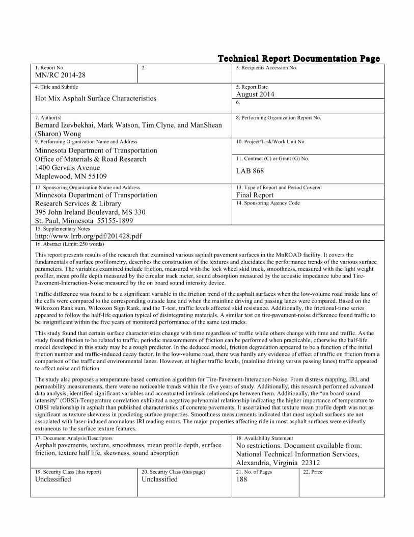
Technical Report Documentation Page 1. Report No. 2. 3. Recipients Accession No. MN/RC 2014-28
4. Title and Subtitle 5. Report Date
Hot Mix Asphalt Surface Characteristics August 2014 6.
7. Author(s) 8. Performing Organization Report No. Bernard Izevbekhai, Mark Watson, Tim Clyne, and ManShean (Sharon) Wong
9. Performing Organization Name and Address 10. Project/Task/Work Unit No. Minnesota Department of Transportation Office of Materials & Road Research 1400 Gervais Avenue Maplewood, MN 55109
11. Contract (C) or Grant (G) No.
LAB 868
12. Sponsoring Organization Name and Address 13. Type of Report and Period Covered Minnesota Department of Transportation Research Services & Library 395 John Ireland Boulevard, MS 330 St. Paul, Minnesota 55155-1899
Final Report 14. Sponsoring Agency Code
15. Supplementary Notes http://www.lrrb.org/pdf/201428.pdf 16. Abstract (Limit: 250 words) This report presents results of the research that examined various asphalt pavement surfaces in the MnROAD facility. It covers the fundamentals of surface profilometry, describes the construction of the textures and elucidates the performance trends of the various surface parameters. The variables examined include friction, measured with the lock wheel skid truck, smoothness, measured with the light weight profiler, mean profile depth measured by the circular track meter, sound absorption measured by the acoustic impedance tube and Tire-Pavement-Interaction-Noise measured by the on board sound intensity device.
Traffic difference was found to be a significant variable in the friction trend of the asphalt surfaces when the low-volume road inside lane of the cells were compared to the corresponding outside lane and when the mainline driving and passing lanes were compared. Based on the Wilcoxon Rank sum, Wilcoxon Sign Rank, and the T-test, traffic levels affected skid resistance. Additionally, the frictional-time series appeared to follow the half-life equation typical of disintegrating materials. A similar test on tire-pavement-noise difference found traffic to be insignificant within the five years of monitored performance of the same test tracks.
This study found that certain surface characteristics change with time regardless of traffic while others change with time and traffic. As the study found friction to be related to traffic, periodic measurements of friction can be performed when practicable, otherwise the half-life model developed in this study may be a rough predictor. In the deduced model, friction degradation appeared to be a function of the initial friction number and traffic-induced decay factor. In the low-volume road, there was hardly any evidence of effect of traffic on friction from a comparison of the traffic and environmental lanes. However, at higher traffic levels, (mainline driving versus passing lanes) traffic appeared to affect noise and friction.
The study also proposes a temperature-based correction algorithm for Tire-Pavement-Interaction-Noise. From distress mapping, IRI, and permeability measurements, there were no noticeable trends within the five years of study. Additionally, this research performed advanced data analysis, identified significant variables and accentuated intrinsic relationships between them. Additionally, the “on board sound intensity” (OBSI)-Temperature correlation exhibited a negative polynomial relationship indicating the higher importance of temperature to OBSI relationship in asphalt than published characteristics of concrete pavements. It ascertained that texture mean profile depth was not as significant as texture skewness in predicting surface properties. Smoothness measurements indicated that most asphalt surfaces are not associated with laser-induced anomalous IRI reading errors. The major properties affecting ride in most asphalt surfaces were evidently extraneous to the surface texture features. 17. Document Analysis/Descriptors 18. Availability Statement Asphalt pavements, texture, smoothness, mean profile depth, surface friction, texture half life, skewness, sound absorption
No restrictions. Document available from: National Technical Information Services, Alexandria, Virginia 22312
19. Security Class (this report) 20. Security Class (this page) 21. No. of Pages 22. Price Unclassified Unclassified 188
Hot Mix Asphalt Surface Characteristics
Final Report
Prepared by:
Bernard Igbafen Izevbekhai Mark Watson
Tim Clyne ManShean (Sharon) Wong
Minnesota Department of Transportation Office of Materials & Road Research
August 2014
Published by:
Minnesota Department of Transportation Research Services & Library
395 John Ireland Boulevard, MS 330 St. Paul, MN 55155
This report represents the results of research conducted by the authors and does not necessarily represent the views or policies of the Minnesota Local Road Research Board and/or the Minnesota Department of Transportation. This report does not contain a standard or specified technique.
The authors, the Minnesota Local Road Research Board and/or the Minnesota Department of Transportation do not endorse products or manufacturers. Trade or manufacturers’ names appear herein solely because they are considered essential to this report.
TABLE OF CONTENTS
ACKNOWLEDGEMENTS .................................................................................................................... XIV
CHAPTER 1 ............................................................................................................................................... 1
INTRODUCTION & DEFINITIONS ...................................................................................................... 1
STUDY OBJECTIVES AND RESEARCH OVERVIEW ........................................................ 2 Study Objectives .................................................................................................................... 2 Research Overview ................................................................................................................ 2
BACKGROUND ........................................................................................................................... 4 Skid Resistance: ..................................................................................................................... 5 Microtexture: ......................................................................................................................... 5 Macrotexture: ........................................................................................................................ 5 Megatexture: .......................................................................................................................... 6 Mean Texture Depth (MTD): ............................................................................................... 6 International Ride Index (IRI): ............................................................................................ 7
MEASURING SURFACE CHARACTERISTICS .................................................................... 7 SURFACE FRICTION ............................................................................................................. 8
British Pendulum Tester (ASTM E 303-93): ...................................................................... 8 Dynamic Friction Tester (DFT), ASTM E 1911: ................................................................ 8 Locked Wheel Skid Trailer Ribbed Tire (ASTM E 501) Smooth Tire (ASTM E 524): . 9 Fixed Slip Devices – Grip Tester (Figure 1.5) (No ASTM Available): ........................... 10
MACROTEXTURE ................................................................................................................ 10
Sand Patch Test ASTM E 965-96:...................................................................................... 10 Circular Track Meter (CTMeter) ASTM E 2157-01: ...................................................... 10 Ultra-Light Inertial Profiler (ULIP) [14]: ......................................................................... 11 Outflow Meter: .................................................................................................................... 11
MEGATEXTURE ................................................................................................................... 11
RUGO Non-Contact Profilometer (developed by the French Laboratory of Roads and Bridges (Figure 1. 7) International Standard – ISO 5725: .............................................. 11
NOISE ...................................................................................................................................... 15

Controlled Pass-by (CPB) and Statistical Pass-by (SPB): ............................................... 15 Close Proximity (CPX) - On Board Sound Intensity (OBSI): ......................................... 16 Impedance Tube (ASTM E-1050 Modified) for In Situ Evaluation Sound Absorption: ............................................................................................................................................... 17 High Speed Laser Systems: ................................................................................................. 18
MODELS AND ANALYSES OF SURFACE CHARACTERISTICS ................................... 20
INTERRELATIONSHIPS AMONG SURFACE CHARACTERISTICS ............................ 24 FRICTION & HMA DESIGN PARAMETERS .................................................................. 24
TEXTURE & NOISE .............................................................................................................. 26
CHAPTER CONCLUDING REMARKS ................................................................................. 28
CHAPTER 2 ............................................................................................................................................. 29
CONSTRUCTION AND INITIAL TESTING OF VARIOUS TEST CELLS ..................................... 29
CHAPTER INTRODUCTION .................................................................................................. 30 CHAPTER OBJECTIVES ..................................................................................................... 31
CELL CONSTRUCTION .......................................................................................................... 31 INTRODUCTION ................................................................................................................... 31
MAINLINE CELLS ................................................................................................................ 34
LOW VOLUME ROAD CELLS ........................................................................................... 36
EXPERIMENTAL TESTING ................................................................................................... 37 TEXTURE ................................................................................................................................ 38
Sand Patch Test: .................................................................................................................. 38 FRICTION ............................................................................................................................... 41
Locked Wheel Skid Trailer (LWST): ................................................................................ 41 Grip Tester: .......................................................................................................................... 46 Dynamic Friction Tester: .................................................................................................... 48
RIDE ......................................................................................................................................... 48
Ames Light Weight Profiler Measurements: .................................................................... 48 SOUND ..................................................................................................................................... 50
Absorption (Impedance Tube): .......................................................................................... 50 Intensity (OBSI):.................................................................................................................. 52
HYDRAULIC CONDUCTIVITY ......................................................................................... 54
Falling Head Permeameter: ................................................................................................ 54 DURABILITY ......................................................................................................................... 56
LTPP Distress Survey Strategy: ......................................................................................... 56
DISCUSSION ON INITIAL TESTING RESULTS OF CONSTRUCTED CELLS ............ 60
CHAPTER 3 ............................................................................................................................................. 62
SEASONAL MEASUREMENTS OF SURFACE: 4TH YEAR CHARACTERISTICS (2012) ........ 62
PERFORMANCE OF SURFACE TREATMENTS ............................................................... 63 Chapter Objectives .............................................................................................................. 63 Chronology of Surface Treatments .................................................................................... 63 ............................................................................................................................................... 66
FRICTION ............................................................................................................................... 74
Locked Wheel Skid Trailer (LWST): ................................................................................ 74 Dynamic Friction Tester: .................................................................................................... 77 Sound Intensity (OBSI): ...................................................................................................... 82
HYDRAULIC CONDUCTIVITY ......................................................................................... 85
DURABILITY ......................................................................................................................... 88
Visual Distress Survey (LTPP):.......................................................................................... 88 Rutting (ALPS): ................................................................................................................... 89
SECTION CONCLUSION ..................................................................................................... 92
CHAPTER 4 ............................................................................................................................................. 95
ADVANCED DATA ANALYSIS ............................................................................................................ 95
BACKGROUND ......................................................................................................................... 96
EVALUATION OF SKEWNESS PROPERTIES SURFACES ............................................. 96
Intensity (OBSI):................................................................................................................ 100 Mean Profile Depth (MPD): ............................................................................................. 101
ANALYTICAL METHOD ................................................................................................... 102
Dependent Variable:.......................................................................................................... 102 Independent Variables ...................................................................................................... 102 Plots of OBSI vs. Mean Profile Depth: ............................................................................ 102 Summary: ........................................................................................................................... 108
STUDY OF PAVEMENT NOISE VERSUS TEMPERATURE .......................................... 109 INTRODUCTION ................................................................................................................. 109
Relationship between Density and Temperature: .......................................................... 110 Definition of Sound Intensity: .......................................................................................... 110 Relationship between Sound Intensity and Temperature: ............................................ 111
APPROACH .......................................................................................................................... 112
Direct Method: ................................................................................................................... 112 Solver Method: ................................................................................................................... 112 Comparison of Data: ......................................................................................................... 112 T-Test: Paired Two Samples for Means: ......................................................................... 113
RESULTS ............................................................................................................................... 113
OBSI vs. Temperature: ..................................................................................................... 113 EFFECT OF TRAFFIC ON OBSI................................................................................... 120
FRICTIONAL PROPERTIES ON ASPHALT PAVEMENT SURFACES ....................... 122 INTRODUCTION ................................................................................................................. 122
Friction Number: ............................................................................................................... 123 Coefficient of Friction: ...................................................................................................... 123 Friction Number vs. Time: ............................................................................................... 124 Comparison of Coefficient of Friction at the Speed of 40km/hr.: ................................. 128 Effect of Traffic on Friction Number: ............................................................................. 129 Effect of Traffic on Skid Resistance: ............................................................................... 130 Friction Number vs. Time: ............................................................................................... 132 Comparison for Coefficient of Friction of Cells at 40km/hr: ........................................ 132 Preliminary Half-life Friction Extrapolations: ............................................................... 133

CHAPTER 5: CONCLUSION & RECOMMENDATIONS .............................................................. 135
CONCLUSION ......................................................................................................................... 136
RECOMMENDATIONS .......................................................................................................... 139
REFERENCES ....................................................................................................................................... 139
LIST OF FIGURES IN TEXT
Figure 1.1 Texture Wavelength Influence on Surface Characteristics [2] ----------------------- 5
Figure 1.2 Microtexture vs. Macrotexture [1] --------------------------------------------------------- 6
Figure 1.3 MnDOT’s Portable Friction Devices [23] ------------------------------------------------- 8
Figure 1.4 Locked Wheel Skid Trailer [23] ------------------------------------------------------------ 9
Figure 1.5 Grip Tester [4] --------------------------------------------------------------------------------- 10
Figure 1.6 Measurement of Texture Depth [23] ------------------------------------------------------ 11
Figure 1.7 RUGO Device and Operating Principle [6] --------------------------------------------- 12
Figure 1.8 Lightweight Inertial Surface Analyzer (LISA) [15] ----------------------------------- 13
Figure 1.9 MnDOT Pavement Management Van [8] ------------------------------------------------ 14
Figure 1.10 DAM, DEK and Dipstick Profile Devices [15] ----------------------------------------- 15
Figure 1.11 MnDOT OBSI Set-Up [20]. ---------------------------------------------------------------- 16
Figure 1.12 Impedance Tube ----------------------------------------------------------------------------- 18
Figure 1.13 FDOT Unit with LMI Technologies, Selcom, High Speed Laser System [21]. - 18
Figure 1.14 RoadSTAR Device [22] --------------------------------------------------------------------- 19
Figure 2.1 MnROAD Facility Map ---------------------------------------------------------------------- 30
Figure 2.2 Location of Test Cells on MnROAD Mainline (ML) ---------------------------------- 31
Figure 2.3 Locations of Test Cells on MnROAD Low Volume Road (LVR) ------------------- 31
Figure 2.4 Typical Sections of Mainline (ML) Test Cells------------------------------------------- 33
Figure 2.5 Typical Sections of Mainline (ML) Test Cells------------------------------------------- 34
Figure 2.6 UTBWC (Left) and X-Section of Porous HMA (Right) ------------------------------ 35
Figure 2.7 Nova Chip Paver --------------------------------------------- Error! Bookmark not defined.
Figure 2.8: Nova Chip Surface (Left) and Warm Mix Surface (Right) ------------------------- 36
Figure 2.9 Sand Patch Field Tests (LEFT) and Test Schematic (RIGHT) --------------------- 39
Figure 2.10 October 2008 Sand Patch Test Results-------------------------------------------------- 40
Figure 2.5 Circular Track Meter Outside Lane (LVR) or Driving Lane Mainline (CTM)
Spring 2009 Results----------------------------------------------------------------------------------- 41
Figure 2.13 October 2008 MnROAD LWST Results for ML-Driving, LVR-Inside Lane -- 43
Figure 2.14 June 2009 MnROAD LWST Results for ML-Driving, LVR-Inside Lane ------- 45
Figure 2.15 June 2009 MnROAD LWST Results for ML-Passing, LVR- Outside Lane ---- 45
Figure 2.16 April 2009 MnROAD Grip Tester Results for ML-Driving, LVR-Inside Lane 47
Figure 2.17 April 2009 MnROAD Grip Tester Results for ML-Passing, LVR-Outside Lane
Figure 2.18 Plot of Average IRI for Driving Lane (in/mi), LISA Results ----------------------- 49
Figure 2.19 Plot of Average IRI for Passing Lane (in/mi), LISA Results ----------------------- 49
Figure 2.20 October 2008 Continuous Ride Results of Cell 3 (Driving Lane, LWP) --------- 50
Original (NCAT) Impedance Tube 2008 -------------------------------------------------------------- 51
Impedance Tube (Base enhanced with Circular Hollow Ring & Hermetic Seal) ------------- 51
Figure 2.21 Sound Impedance Tube -------------------------------------------------------------------- 51
Figure 2.22 Absorption Ratios for Selected HMA Surface Types -------------------------------- 52
Figure 2.23 On Board Sound Intensity Test Setup and Microphone Close Up View -------- 52
Figure 2.24 On Board Sound Intensity Test Results Passing Lane ------------------------------ 53
Figure 2.25 On Board Sound Intensity Test Results Driving Lane ------------------------------ 53
Figure 2.26 A-Weighted Sound Intensity -------------------------------------------------------------- 54
Figure 2.27 Cascaded Field Permeameter ------------------------------------------------------------- 55
Figure 2.28 Hydraulic Conductivity of Non-Porous HMA----------------------------------------- 55
Figure 2.29 Hydraulic Conductivity of Porous HMA ----------------------------------------------- 56
Figure 2.30 Porous HMA (Cell 86 LEFT, Cell 88 RIGHT), August 2009 ---------------------- 57
Figure 2.31 4.75 mm Aggregate Asphalt (Cell 6), August 2009 ----------------------------------- 57
Figure 3.1 Typical Sections of Mainline (ML) Test Cells as at 2011 ----------------------------- 63
Figure 3.3 Ultra-Thin Bonded Wearing Coarse [Left], Warm Mix Asphalt [Right] --------- 66
Figure 3.4 4.75 Taconite [Left] and Cross-Section of Porous HMA [Right] ------------------- 67
Figure 3.6 History of CTM Data (2009-2012) --------------------------------------------------------- 68
Figure 3.7 2012 Cell 2 CTM Data by Station(110900=1109+00) --------------------------------- 69
Figure 3.8 2012 Cell 3 CTM Data by Station(111500=1115+00) ---------------------------------- 69
Figure 3.9 2012 Cell 4 CTM Data by Station (112100=1121+00) --------------------------------- 70
Figure 3.10 2012 Cell 19 CTM Data by Station(121800=1218+00) ------------------------------- 70
Figure 3.11 2012 Cell 22 CTM Data by Station (123600=236+00) ------------------------------- 71
Figure 3.12 2012 Cell 24 CTM Data by Station(15800=158+00) ---------------------------------- 71
Figure 3.13 2012 Cell 27 CTM Data by Station(17600=176+00) ---------------------------------- 72
Figure 3.14 2012 Cell 86 CTM Data by Station(16632=166+32) --------------------------------- 72
Figure 3.15 2012 Cell 87 CTM Data by Station(16860=168+60) ---------------------------------- 73
Figure 3.16 2012 Cell 88 CTM Data by Station (17084=170+84) -------------------------------- 73
Figure 3. 17 History of Skid Trailer Data, Ribbed Tire -------------------------------------------- 75
Figure 3.18 2012 Mainline Skid Trailer Data -------------------------------------------------------- 76
Figure 3.19 2012 Low Volume Road Skid Trailer Data ------------------------------------------- 76
Figure 3.20 History of DFT Data at 20 km/hr -------------------------------------------------------- 78
Figure 3.21 History of DFT Data at 80 km/hr -------------------------------------------------------- 78
Figure 3.22 2012 DFT Data vs. Speed (1 mph=1.6 km/hr ------------------------------------------ 79
Figure 3.23 LVR Cell 24 DFT Data over Fog Seals-------------------------------------------------- 79
Figure 3.24 History of LISA Ride Quality Values (Driving/Inside Lane) ---------------------- 80
Figure 3.25 Mainline 2012 LISA Measurements ----------------------------------------------------- 81
Figure 3.26 Low Volume Road 2012 LISA Measurements ---------------------------------------- 82
Figure 3. 27 History of OBSI Measurements (Driving/Inside Lane) ----------------------------- 83
Figure 3.28 2012 Mainline OBSI Data ----------------------------------------------------------------- 84
Figure 3.29 2012 Low Volume Road OBSI Data ----------------------------------------------------- 84
Figure 3. 30 Field Permeameter ------------------------------------------------------------------------- 85
Figure 3.31 History of Permeability Measurements ------------------------------------------------- 86
Figure 3.32 2012 Hydraulic Conductivity (Inside Lane) ------------------------------------------- 87
Figure 3.33 2012 Hydraulic Conductivity (Outside Lane) ----------------------------------------- 87
Figure 3.34 Automated Laser Profile System (ALPS) ---------------------------------------------- 90
Figure 3.35 History of Average Mainline Rut Depths ---------------------------------------------- 91
Figure 3.36 History of Average Low Volume Road Rut Depths ---------------------------------- 91
Figure 4.1 CTM and PARSER ICONS ---------------------------------------------------------------- 97
Figure 4.2 Layout Graphs and Probability Density Function Graphs [57] -------------------- 99
Figure 4.3 Example of graph plotted for determining the suitable segments ---------------- 101
Figure 4.4 Plot of OBSI vs. MPD for driving lane at mainline ---------------------------------- 103
Figure 4.5 Plot of OBSI vs. MPD for passing lane at mainline ---------------------------------- 103
Figure 4.6 Plot of OBSI vs. MPD for inside lane at LVR ----------------------------------------- 104
Figure 4.7 Plot of OBSI vs. MPD for outside lane at LVR --------------------------------------- 104
Figure 4.8 Plot of OBSI vs. MPD for both lane at mainline ------------------------------------- 105
Figure 4.9 Plot of OBSI vs. Skewness for driving lane at mainline ---------------------------- 106
Figure 4.10 Plot of OBSI vs. Skewness for passing lane at mainline --------------------------- 106
Figure 4.11 Plot of OBSI vs. Skewness for inside lane at LVR ---------------------------------- 107
Figure 4.12 Plot of OBSI vs. Skewness for outside lane at LVR -------------------------------- 107
Figure 4.13 Plot of OBSI vs. MPD for both lane at mainline and LVR ----------------------- 108
Figure 4.14: OBSI versus Temperature plot -------------------------------------------------------- 111
Figure 4.15: Comparison of Linear Trend line and Power Trend line for cell 1 ------------ 114
Figure 4.16 Plot of OBSI Difference versus Temperature for cell 1 --------------------------- 114
Figure 4.17 Plot of OBSI Difference versus Temperature for cell 2 --------------------------- 115
Figure 4.18 Plot of OBSI Difference versus Temperature for cell 3 --------------------------- 115
Figure 4.19 Plot of OBSI Difference versus Temperature for cell 4 --------------------------- 116
Figure 4.20 Plot of OBSI Difference versus Temperature for cell 15 -------------------------- 116
Figure 4.21 Plot of OBSI Difference versus Temperature for cell 19 -------------------------- 117
Figure 4.22 Plot of OBSI Difference versus Temperature for Cell 20 ------------------------- 117
Figure 4.23 Plot of OBSI Difference versus Temperature for cell 22 -------------------------- 118
Figure 4.24 Plot of OBSI Difference versus Temperature for cell 70 -------------------------- 118
Figure 4.25 Data for 9 Test Cells ---------------------------------------------------------------------- 119
Figure 4.26 Schematic of adhesion and hysteresis component of rubber friction [58] ----- 123
Figure 4.27 Forces on a rolling tire ------------------------------------------------------------------- 124
Figure 4.28 Friction Number vs. Time for Cell 1 Driving Lane -------------------------------- 125
Figure 4.29 Friction Number vs. Time for Cell 2 Driving Lane -------------------------------- 126
Figure 4.30 Friction Number vs. Time for Cell 3 Driving Lane -------------------------------- 127
Figure 4.31 Friction Number vs. Time for Cell 4 Driving Lane -------------------------------- 128
Figure 4.32 Comparison of Coefficient of Friction With DFT ---------------------------------- 129
LIST OF TABLES
Table 1.1 Properties and Characteristics measured by RoadSTAR [22] ----------------------- 20
Table 1.2 Classification of Different Pavement Categories using CPB -------------------------- 22
Table 1.3 Pavement Test Sections Used in CalTrans Study --------------------------------------- 26
Table 1.4 Data Collection and Tests -------------------------------------------------------------------- 27
Table 2.1 Location HMA Surface Allocation --------------------------------------------------------- 32
Table 2.2 2008 HMA Paving Dates ---------------------------------------------------------------------- 33
Table 2.3 2008 Average Density and Air Void Results for HMA Cores ------------------------ 37
Table 2.4 Tests Used to Characterize Initial HMA Surface Characteristics ------------------- 38
Table 2.5 October 2008 LWST Results ML-Driving, LVR-Inside Lane ------------------------ 43
Table 2.6 June 2009 LWST Results --------------------------------------------------------------------- 44
Table 2.1 (Cont’d) June 2009 LWST Results --------------------------------------------------------- 45
Table 2.2: Distress Survey of Test Cells Using LTPP Procedure --------------------------------- 58
Table 2.3: LTPP Distress Survey of Test Cells (Cont.) --------------------------------------------- 59
Table 3.1 Chip Seal Surface Treatment Gradation -------------------------------------------------- 66
Table 3.3 Descriptive Statistics for Skid Trailer Data 2009-2012 (Ribbed Tire) -------------- 74
Table 3.4 LTPP Distress Ratings for Asphalt Concrete Surfaces -------------------------------- 88
Table 3.5 Fall 2012 LTPP Distress Surveys ----------------------------------------------------------- 89
Table 4.1 R2 value for mainline and LVR according to the lanes ------------------------------ 108
Table 4.2 Power trend line equation for all cells --------------------------------------------------- 119
Table 4.3: Summary for Effect of Traffic on OBSI (Statistical Hypothesis Tests) --------- 121
Table 4.4: Results for Effects of Traffics on OBSI Difference ---------------------------------- 121
Table 4.5 Data Tabulation of FN Ribbed and Smooth for Cell 1 Driving Lane ------------- 125
Table 4.6 Data Tabulation of FN Ribbed and Smooth for Cell 2 Driving Lane ------------- 126
Table 4.7 Data Tabulation of FN Ribbed and Smooth for Cell 3 Driving Lane ------------- 127
Table 4.8 Data Tabulation for FN Ribbed and Smooth for Cell 4 Driving Lane ----------- 128
Table 4.9 Range of Coefficient of Friction for Cell 3, 4, 19, 22 ---------------------------------- 129
Table 4.10: P-values for Friction Number at 95% Confidence Level ------------------------- 130
Table 4.11: Summary for Effect of Traffics on FN: (Statistical Hypothesis Tests) --------- 131
Table 4.12: Results for Effects of Traffic on Frictional Resistance ---------------------------- 131

Table 4.13 Summary of half-life analysis for test cell 2, 3, 4 and 27 --------------------------- 134
ACKNOWLEDGEMENTS Authors are indebted to the Federal Highway Administration, Local Road Research
Board and MnDOT for facilitating this study. John Pantelis, Eddie Johnson and
Steve Olson performed the surface characteristics measurements.
Bernard Igbafen Izevbekhai, P.E., Ph.D.
Research Operations Engineer
Minnesota Department of Transportation
1400 Gervais Avenue Maplewood MN 55109
E-mail: [email protected]
Phone: 651 3665454 Fax: 6513665461
July 2014

1
CHAPTER 1
INTRODUCTION & DEFINITIONS
2
STUDY OBJECTIVES AND RESEARCH OVERVIEW Study Objectives
Prior to this study, MnDOT needed to know how various asphalt surface types perform over
time. It therefore initiated this study to evaluate frictional properties, texture configurations,
texture durability, ride quality, acoustic impedance and noise characteristics of asphalt surfaces.
Study was aimed at ascertaining optimal and economic textures or surfaces that optimize
durability, quietness, friction and ride quality. While 4 years were not considered sufficient to
accomplish all the objectives particularly in long terms, it aims at accentuating the short-term
properties for extrapolations where tenable. Additionally, this study served at the barest
minimum as a springboard for continuation of research on asphalt surfaces.
Research Overview
The work done in this research is best accentuated through the tasks outlined and performed.
Task 1 performed a literature review detailing state-of-the-practice and state-of-the-art
techniques for measuring, analyzing, and modeling pavement surface characteristics. The
interrelationships between noise, texture, ride, friction, and durability will be reviewed.
Task 2 described test section construction and initial monitoring Construction on several
MnROAD test cells used for this study took place during the summer of 2008. Immediately after
construction texture, friction, noise and ride measurements were performed. This served as
baseline measurements for comparison in subsequent data collection efforts. Several pieces of
equipment and software acquired to assist in data collection and analysis in the study were
discussed.
Deliverable for Task 2: PowerPoint presentation and summary report.
Task 3 involved Subcontracts for Additional Measurements and Analysis
Outside researchers/consultants will be hired to perform additional surface characteristic
measurements that MnDOT is not currently equipped to perform. These measurements included
statistical pass by (noise), sound absorption, Robotex (3-D surface texture), rolling resistance
(fuel efficiency), and others. In addition, consultants may be hired to perform advanced data
3
analysis on certain surface characteristic measurements (e.g., the effect of texture on sound
absorption). Reports were rendered for each task.
Task 4 performed and discussed seasonal measurements of surface characteristics (2009)
The surface characteristics measurements performed twice per year for four years quantified
seasonal variation. Noise was measured with On Board Sound Intensity (OBSI) protocol and the
sound absorption tube. Texture was measured with the sand volumetric technique or a laser
device ASTM E-2157. Ride was measured with the triple and single laser of the lightweight
profiler. Friction was measured with a skid trailer according to ASTM E 274 procedure, the
dynamic friction tester, and other devices as they became available. Durability was assessed in
terms of pavement raveling and cracking according to a MnDOT-modified LTPP distress survey.
Task 5 Performed and discussed Seasonal Measurements of Surface Characteristics (2010)
Task 6 performed and discussed Seasonal Measurements of Surface Characteristics (2011)
Task 7 performed and discussed Seasonal Measurements of Surface Characteristics (2012)
Task 8 was the analytical part of the study where the data from tasks 2-7 were analyzed
mathematically and statistically. Among many other things, this task developed a process for
extracting skewness from the texture data using a software PARSER and analyzed it to ascertain
the importance of the skewness parameter in asphalt surfaces. Other analysis included the
influence of traffic on Ride friction and noise. Additionally, friction degradation was examined
in the light of analysis of experimental data. The field data collected during the project was
analyzed graphically. Relationships between the various pavement surface characteristics will be
identified and characterized. Deliverable for Task 8: PowerPoint presentation and summary
report.
Task 9 performed a technical summary for Deployment and Implementation of the lessons
learned in this study. This technical brief will be written and distributed to interested parties both
locally and nationally. Where applicable, revised protocols and/or specifications will be
4
proposed for asphalt mixtures (MnDOT Bituminous Office) and noise mitigation techniques
(MnDOT Office of Environmental Services).
Task 10 performed a compilation of the draft final report on this study. For the avoidance of
redundancy, this final report included the background and state of the art in one chapter,
construction of various textures in the next chapter followed by the fourth year performance
report in the third chapter. It was not deemed necessary to enunciate the previous years’
performance since these were reflected in the fourth year time series. The data analysis was the
bulk of the final report and was presented in the 4th chapter. The 5th chapter presents the
conclusion and recommendations.
BACKGROUND Pavement surface characteristics are composed of several different interrelated parameters,
which will be defined later. These parameters include texture, ride, friction, noise and durability.
Often times the same measured parameter obtained using one device does not necessarily
correlate with the same parameter measurements obtained using another device – this has led to
recent efforts to harmonize results using international indexes such as the international friction
index (IFI that combines friction value and a speed number) and the international ride index
(IRI). These indexes have helped researchers to quantify and compare results obtained in
different locations, with different equipment and under different conditions. Texture and ride are
commonly evaluated using spectral analysis, which can be described using two parameters: a
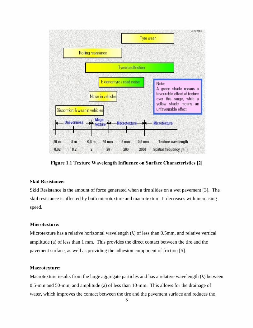
horizontal component, or wavelength (λ) and a vertical component, or amplitude (a). Figure 1.1
below shows typical influence of different texture wavelengths on pavement surface
characteristics. Note that some characteristics such as noise, friction, and splash and spray are
affected by the same wavelength.
5
Figure 1.1 Texture Wavelength Influence on Surface Characteristics [2]
Skid Resistance:
Skid Resistance is the amount of force generated when a tire slides on a wet pavement [3]. The
skid resistance is affected by both microtexture and macrotexture. It decreases with increasing
speed.
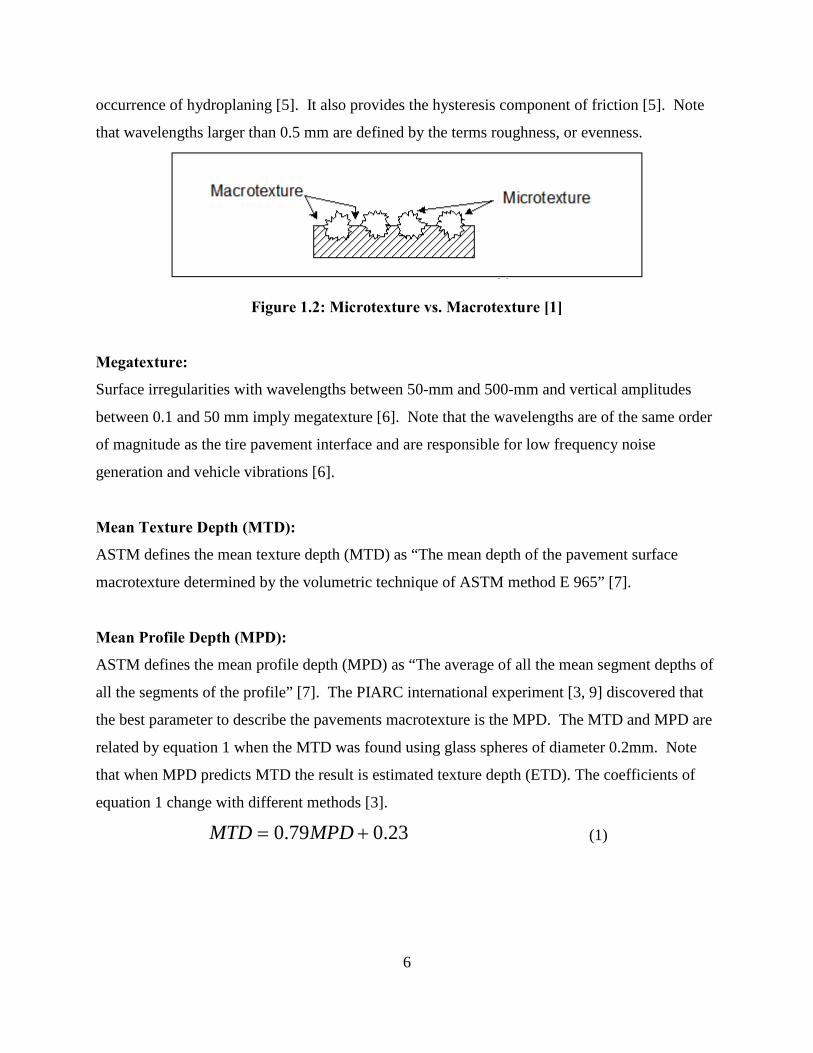
Microtexture:
Microtexture has a relative horizontal wavelength (λ) of less than 0.5mm, and relative vertical
amplitude (a) of less than 1 mm. This provides the direct contact between the tire and the
pavement surface, as well as providing the adhesion component of friction [5].
Macrotexture:
Macrotexture results from the large aggregate particles and has a relative wavelength (λ) between
0.5-mm and 50-mm, and amplitude (a) of less than 10-mm. This allows for the drainage of
water, which improves the contact between the tire and the pavement surface and reduces the
6
occurrence of hydroplaning [5]. It also provides the hysteresis component of friction [5]. Note
that wavelengths larger than 0.5 mm are defined by the terms roughness, or evenness.
Figure 1.2: Microtexture vs. Macrotexture [1]
Megatexture:
Surface irregularities with wavelengths between 50-mm and 500-mm and vertical amplitudes
between 0.1 and 50 mm imply megatexture [6]. Note that the wavelengths are of the same order
of magnitude as the tire pavement interface and are responsible for low frequency noise
generation and vehicle vibrations [6].
Mean Texture Depth (MTD):
ASTM defines the mean texture depth (MTD) as “The mean depth of the pavement surface
macrotexture determined by the volumetric technique of ASTM method E 965” [7].
Mean Profile Depth (MPD):
ASTM defines the mean profile depth (MPD) as “The average of all the mean segment depths of
all the segments of the profile” [7]. The PIARC international experiment [3, 9] discovered that
the best parameter to describe the pavements macrotexture is the MPD. The MTD and MPD are
related by equation 1 when the MTD was found using glass spheres of diameter 0.2mm. Note
that when MPD predicts MTD the result is estimated texture depth (ETD). The coefficients of
equation 1 change with different methods [3].
23.079.0 += MPDMTD (1)
7
International Friction Index:
The International Friction Index (IFI) is composed of a friction number (F60) and a speed
constant (Sp) [3]. Sp relates to the macrotexture [1] while friction value and the speed constant
[2] [3] generate F60.
TXbaS p ∗+= (1) TXCeFRSBAF pSS
∗+∗∗+=−60
60 (2)
Where:
• a and b are constants determined for each specific texture TX
• FRS is the measurement of friction by a specific device at speed S
• A, B and C are device specific constants tabulated in ASTM E-1960 [10]
• C is zero for smooth tires, and non-zero for ribbed, or patterned tires
International Ride Index (IRI):
A MnDOT report [8] defines the international Ride Index (IRI) as “The amount of vertical
movement a vehicle would experience over a given horizontal stretch of road” [8]. A clearer
definition actually reflects the vertical displacement as a function of vertical acceleration of the
quarter car travelling on that profile at 50 miles per hour. An extremely rough spot on a smooth
road would produce little change in IRI for a long analysis section.
MEASURING SURFACE CHARACTERISTICS Often times it is insufficient to measure only one surface characteristic, and it becomes necessary
to employ multiple tests to describe the pavement surface accurately [3]. In addition to
measuring multiple characteristics, testing for surface characteristics must account for the
changes due to temperature and seasons. There are also short-term changes, for example, when
rain events wash off dust and oil accumulations from pavement surfaces, friction numbers
(before and after this event) vary [3]. Special consideration must also be given to the equipment
to ensure proper calibration. Often times it is difficult to compare measurements of the same
characteristic made with two different devices. For instance, the Dynamic Friction Tester (DFT)
generates a DFT number while the Lockwheel skid trailer generates a friction number (FN).
8
Correlation of one to the other for measurement taken on the same spot presents challenges. The
next subsection describes some of the equipment and technologies used in this study.
SURFACE FRICTION
There currently is no system available to measure microtexture profiles at highway speeds [3]
therefore these portable devices are used.
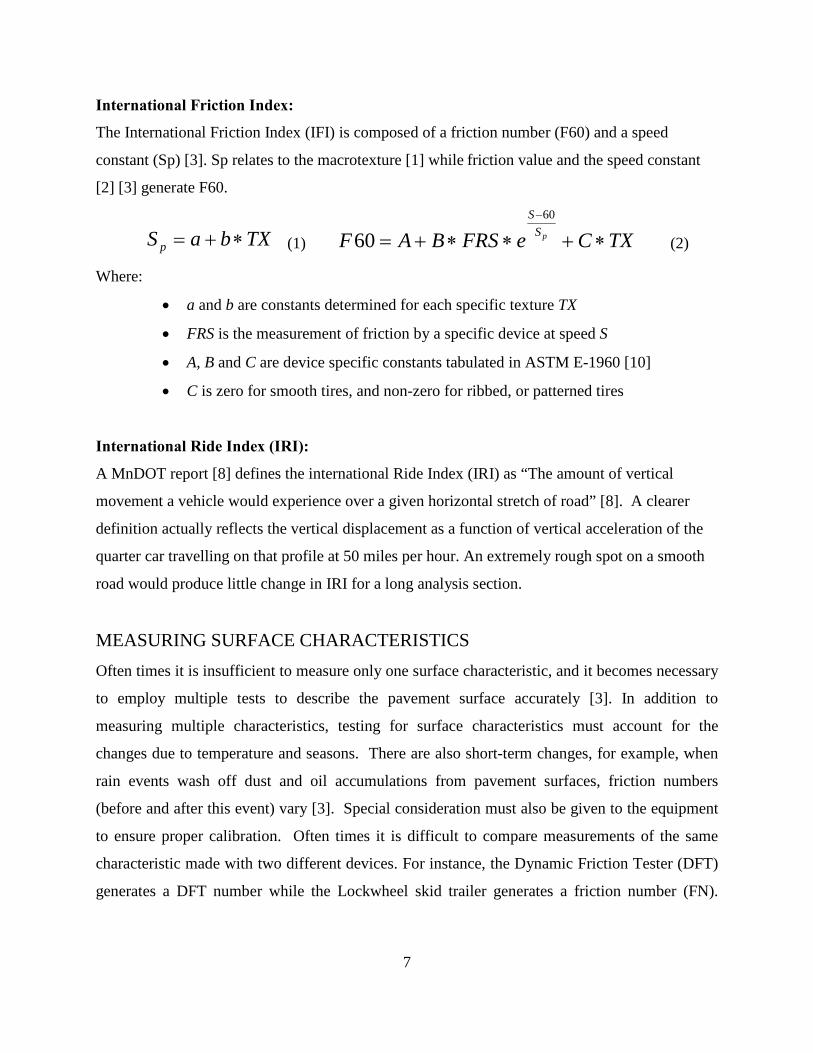
British Pendulum Tester (ASTM E 303-93):
The relatively simple portable device that has field and lab application has been in operation
since 1960 [3]. A slider of known potential energy and low slip speed makes contact with the
pavement over a fixed distance; the loss of energy due to the contact with the surface is due to
friction. The results are reported in terms of a British Pendulum Number that can be used as a
surrogate for microtexture. Preliminary measurements were made with this device but
researchers were not certain of the repeatability of results are those were largely dependent on
the condition of the plastic pads that often needed replacement.
Dynamic Friction Tester (DFT), ASTM E 1911:
The Dynamic Friction Tester (DFT) shown in Figure 1.3 below consists of three rubber sliders,
positioned on a disk of diameter 13.75 in, that are suspended above the pavement surface. When
the tangential velocity of the sliders reaches 90 km/hr water is applied to the surface and the
sliders make contact with the pavement.
Figure 1.3 MnDOT’s Portable Friction Devices [23]
a) British Pendulum b) DFT Contact Base c) DFT Front/side View
9
A computer takes friction measurements across a range of speeds as the sliders slow to a stop. A
DFT value obtained at 20 km/hr, along with texture measurement provides a good indication of
IFI [3].
Locked Wheel Skid Trailer Ribbed Tire (ASTM E 501) Smooth Tire (ASTM E 524):
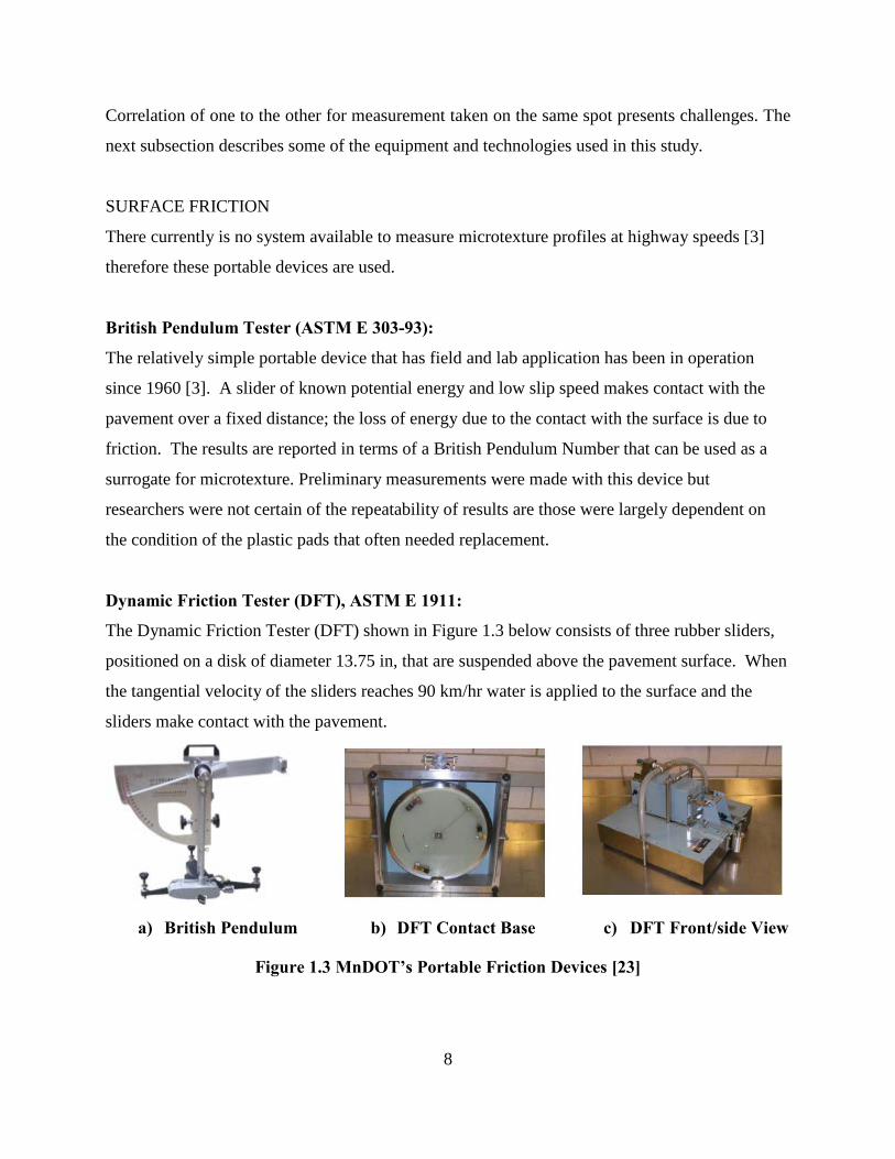
The LWST test method is the most popular in the U.S. [3] (Figure 1.4). Both LWST testing
methods are identical except in the specifications of the test tire; either a ribbed or a smooth tread
tire can be used. The locked wheel system produces a slip speed (speed of the test tire relative to
the speed of the vehicle) equal to that of the test vehicle (see Figure 1. 4), or a 100% slip
condition. The brake is applied to the testing wheel and the resulting constant force is measured
for an average of 1 second after the wheel is locked. Since the test does not give a continuous
measurement, the Standard [11] requires at least five lockups in a uniform test section. The
results are reported as a skid number, which is 100 times the friction value. Although most states
use the ribbed tire, there has been an increased interest in use of the smooth tire. Furthermore,
even though friction testing often times accompanies accident investigations, the friction values
obtained from the tests are intended for comparison with other pavements, or to chart the change
with time, and are insufficient to determine vehicle stopping distances [11]. The ribbed tire is
primarily influenced by microtexture and the smooth tire is primarily influenced by macrotexture
[3].
Figure 1.4-Locked Wheel Skid Trailer [23]
10
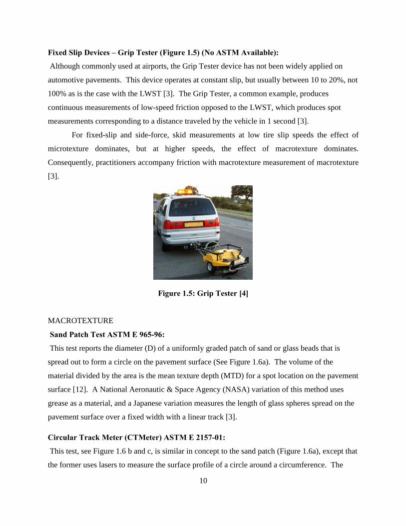
Fixed Slip Devices – Grip Tester (Figure 1.5) (No ASTM Available):
Although commonly used at airports, the Grip Tester device has not been widely applied on
automotive pavements. This device operates at constant slip, but usually between 10 to 20%, not
100% as is the case with the LWST [3]. The Grip Tester, a common example, produces
continuous measurements of low-speed friction opposed to the LWST, which produces spot
measurements corresponding to a distance traveled by the vehicle in 1 second [3].
For fixed-slip and side-force, skid measurements at low tire slip speeds the effect of
microtexture dominates, but at higher speeds, the effect of macrotexture dominates.
Consequently, practitioners accompany friction with macrotexture measurement of macrotexture
[3].
Figure 1.5: Grip Tester [4]
MACROTEXTURE
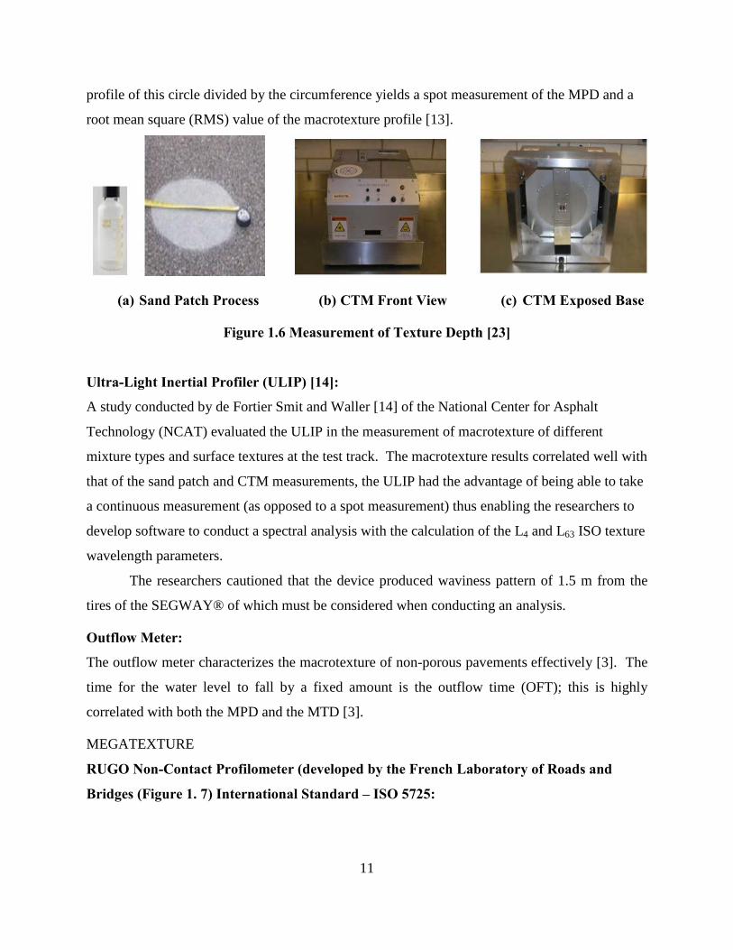
Sand Patch Test ASTM E 965-96:
This test reports the diameter (D) of a uniformly graded patch of sand or glass beads that is
spread out to form a circle on the pavement surface (See Figure 1.6a). The volume of the
material divided by the area is the mean texture depth (MTD) for a spot location on the pavement
surface [12]. A National Aeronautic & Space Agency (NASA) variation of this method uses
grease as a material, and a Japanese variation measures the length of glass spheres spread on the
pavement surface over a fixed width with a linear track [3].
Circular Track Meter (CTMeter) ASTM E 2157-01:
This test, see Figure 1.6 b and c, is similar in concept to the sand patch (Figure 1.6a), except that
the former uses lasers to measure the surface profile of a circle around a circumference. The
11
profile of this circle divided by the circumference yields a spot measurement of the MPD and a
root mean square (RMS) value of the macrotexture profile [13].
Figure 1.6 Measurement of Texture Depth [23]
(a) Sand Patch Process (b) CTM Front View (c) CTM Exposed Base
Ultra-Light Inertial Profiler (ULIP) [14]:
A study conducted by de Fortier Smit and Waller [14] of the National Center for Asphalt
Technology (NCAT) evaluated the ULIP in the measurement of macrotexture of different
mixture types and surface textures at the test track. The macrotexture results correlated well with
that of the sand patch and CTM measurements, the ULIP had the advantage of being able to take
a continuous measurement (as opposed to a spot measurement) thus enabling the researchers to
develop software to conduct a spectral analysis with the calculation of the L4 and L63 ISO texture
wavelength parameters.
The researchers cautioned that the device produced waviness pattern of 1.5 m from the
tires of the SEGWAY® of which must be considered when conducting an analysis.
Outflow Meter:
The outflow meter characterizes the macrotexture of non-porous pavements effectively [3]. The
time for the water level to fall by a fixed amount is the outflow time (OFT); this is highly
correlated with both the MPD and the MTD [3].
MEGATEXTURE
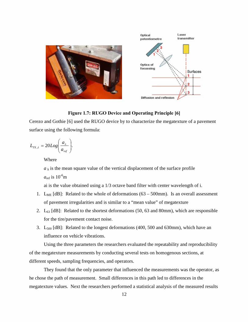
RUGO Non-Contact Profilometer (developed by the French Laboratory of Roads and
Bridges (Figure 1. 7) International Standard – ISO 5725:
12
Figure 1.7: RUGO Device and Operating Principle [6]
Cerezo and Gothie [6] used the RUGO device by to characterize the megatexture of a pavement
surface using the following formula:
=
refTX a
aLogL λ
λ 20, .
Where
a λ is the mean square value of the vertical displacement of the surface profile
aref is 10-6m
ai is the value obtained using a 1/3 octave band filter with center wavelength of i.
1. LME [dB]: Related to the whole of deformations (63 – 500mm). Is an overall assessment
of pavement irregularities and is similar to a “mean value” of megatexture
2. L63 [dB]: Related to the shortest deformations (50, 63 and 80mm), which are responsible
for the tire/pavement contact noise.
3. L500 [dB]: Related to the longest deformations (400, 500 and 630mm), which have an
influence on vehicle vibrations.
Using the three parameters the researchers evaluated the repeatability and reproducibility
of the megatexture measurements by conducting several tests on homogenous sections, at
different speeds, sampling frequencies, and operators.
They found that the only parameter that influenced the measurements was the operator, as
he chose the path of measurement. Small differences in this path led to differences in the
megatexture values. Next the researchers performed a statistical analysis of the measured results
13
following ISO 5725-2 which led them to conclude that the megatexture measurement with the
RUGO device had good accuracy. They noted that the next step in the research process was to
correlate the megatexture measurements with noise measurements [6].
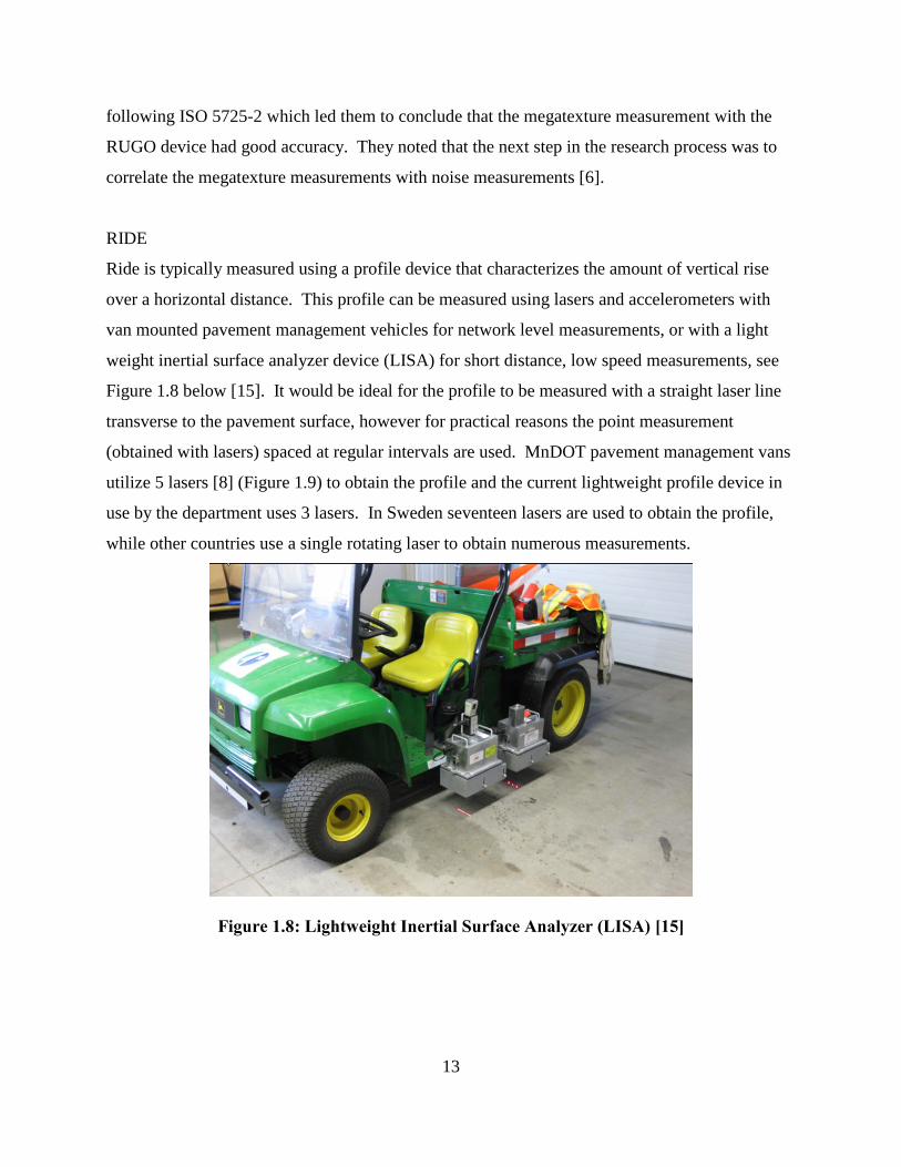
RIDE
Ride is typically measured using a profile device that characterizes the amount of vertical rise
over a horizontal distance. This profile can be measured using lasers and accelerometers with
van mounted pavement management vehicles for network level measurements, or with a light
weight inertial surface analyzer device (LISA) for short distance, low speed measurements, see
Figure 1.8 below [15]. It would be ideal for the profile to be measured with a straight laser line
transverse to the pavement surface, however for practical reasons the point measurement
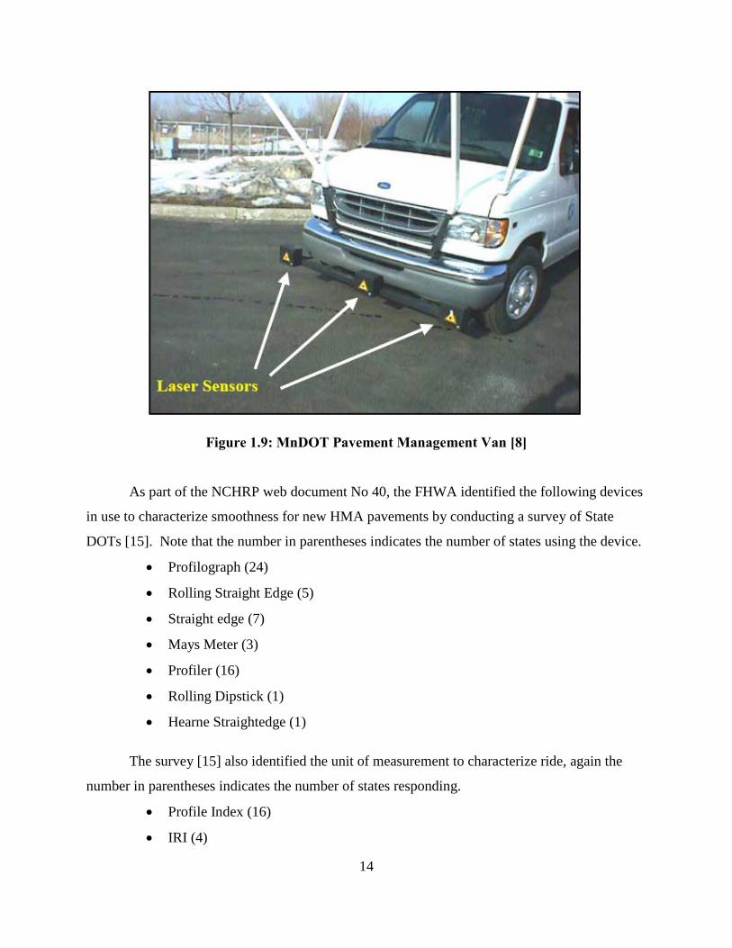
(obtained with lasers) spaced at regular intervals are used. MnDOT pavement management vans
utilize 5 lasers [8] (Figure 1.9) to obtain the profile and the current lightweight profile device in
use by the department uses 3 lasers. In Sweden seventeen lasers are used to obtain the profile,
while other countries use a single rotating laser to obtain numerous measurements.
Figure 1.8: Lightweight Inertial Surface Analyzer (LISA) [15]
14
Figure 1.9: MnDOT Pavement Management Van [8]
As part of the NCHRP web document No 40, the FHWA identified the following devices
in use to characterize smoothness for new HMA pavements by conducting a survey of State
DOTs [15]. Note that the number in parentheses indicates the number of states using the device.
• Profilograph (24)
• Rolling Straight Edge (5)
• Straight edge (7)
• Mays Meter (3)
• Profiler (16)
• Rolling Dipstick (1)
• Hearne Straightedge (1)
The survey [15] also identified the unit of measurement to characterize ride, again the
number in parentheses indicates the number of states responding.
• Profile Index (16)
• IRI (4)
15
• Straight Edge Variability (6)
• Other (6)
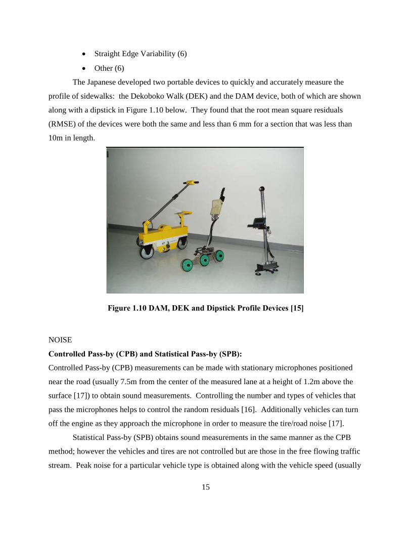
The Japanese developed two portable devices to quickly and accurately measure the
profile of sidewalks: the Dekoboko Walk (DEK) and the DAM device, both of which are shown
along with a dipstick in Figure 1.10 below. They found that the root mean square residuals
(RMSE) of the devices were both the same and less than 6 mm for a section that was less than
10m in length.
Figure 1.10 DAM, DEK and Dipstick Profile Devices [15]
NOISE
Controlled Pass-by (CPB) and Statistical Pass-by (SPB):
Controlled Pass-by (CPB) measurements can be made with stationary microphones positioned
near the road (usually 7.5m from the center of the measured lane at a height of 1.2m above the
surface [17]) to obtain sound measurements. Controlling the number and types of vehicles that
pass the microphones helps to control the random residuals [16]. Additionally vehicles can turn
off the engine as they approach the microphone in order to measure the tire/road noise [17].
Statistical Pass-by (SPB) obtains sound measurements in the same manner as the CPB
method; however the vehicles and tires are not controlled but are those in the free flowing traffic
stream. Peak noise for a particular vehicle type is obtained along with the vehicle speed (usually
16
with a radar device), this information is then used to predict the average noise level of a
particular vehicle group at a given reference speed within a certain confidence interval
(determined by the sample size) [17].
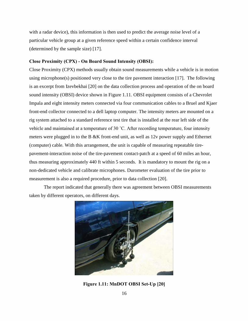
Close Proximity (CPX) - On Board Sound Intensity (OBSI):
Close Proximity (CPX) methods usually obtain sound measurements while a vehicle is in motion
using microphone(s) positioned very close to the tire pavement interaction [17]. The following
is an excerpt from Izevbekhai [20] on the data collection process and operation of the on board
sound intensity (OBSI) device shown in Figure 1.11. OBSI equipment consists of a Chevrolet
Impala and eight intensity meters connected via four communication cables to a Bruel and Kjaer
front-end collector connected to a dell laptop computer. The intensity meters are mounted on a
rig system attached to a standard reference test tire that is installed at the rear left side of the
vehicle and maintained at a temperature of 30 ˚C. After recording temperature, four intensity
meters were plugged in to the B &K front-end unit, as well as 12v power supply and Ethernet
(computer) cable. With this arrangement, the unit is capable of measuring repeatable tire-
pavement-interaction noise of the tire-pavement contact-patch at a speed of 60 miles an hour,
thus measuring approximately 440 ft within 5 seconds. It is mandatory to mount the rig on a
non-dedicated vehicle and calibrate microphones. Durometer evaluation of the tire prior to
measurement is also a required procedure, prior to data collection [20].
The report indicated that generally there was agreement between OBSI measurements
taken by different operators, on different days.
Figure 1.11: MnDOT OBSI Set-Up [20]
17
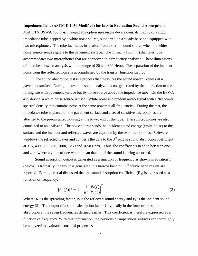
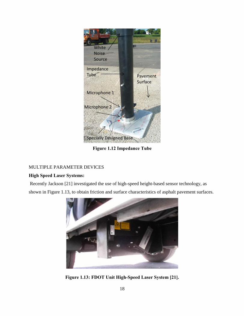
Impedance Tube (ASTM E-1050 Modified) for In Situ Evaluation Sound Absorption:
MnDOT’s BSWA 435 in-situ sound absorption measuring device consists mainly of a rigid
impedance tube, capped by a white noise source, supported on a steady base and equipped with
two microphones. The tube facilitates insulation from exterior sound source when the white
noise source sends signals to the pavement surface. The 11 inch (100 mm) diameter tube
accommodates two microphones that are connected to a frequency analyzer. These dimensions
of the tube allow an analysis within a range of 20 and 800 Hertz. The separation of the incident
noise from the reflected noise is accomplished by the transfer function method.
The sound absorption test is a process that measures the sound absorptiveness of a
pavement surface. During the test, the sound analyzed is not generated by the interaction of the
rolling tire with pavement surface but by noise source above the impedance tube. On the BSWA
425 device, a white noise source is used. White noise is a random audio signal with a flat power
spectral density that contains noise at the same power at all frequencies. During the test, the
impedance tube is placed on the pavement surface and a set of sensitive microphones are
attached to the pre-installed housing at the lower end of the tube. These microphones are also
connected to an analyzer. The noise source sends the incident sound energy (white noise) to the
surface and the incident and reflected waves are captured by the two microphones. Software
windows the reflected waves and converts the data to the 3rd octave sound absorption coefficient
at 315, 400, 500, 750, 1000, 1250 and 1650 Hertz. Thus, the coefficients need to between one
and zero where a value of one would mean that all of the sound is being absorbed.
Sound absorption output is generated as a function of frequency as shown in equation 1
(below). Ordinarily, the result is generated in a narrow band but 3rd octave band results are
reported. Berengier et al discussed that the sound absorption coefficient (Rp) is expressed as a
function of frequency:
|𝑅𝑃(𝑓)|2 = 1 −1𝐾𝑟2
�𝑃𝑟(𝑓)𝑃𝑑(𝑓)
�2
(3)
Where: Kr is the spreading factor, Pr is the reflected sound energy and Pd is the incident sound
energy [3]. The output of a sound absorption factor is typically in the form of the sound
absorption at the seven frequencies defined earlier. This coefficient is therefore expressed as a
function of frequency. With this information, the pervious or impervious surfaces can thoroughly
be analyzed to evaluate acoustical properties.
18
Figure 1.12 Impedance Tube
White Noise Source
Impedance Tube Pavement
Surface
Microphone 2
Microphone 1
Specially Designed Base
MULTIPLE PARAMETER DEVICES
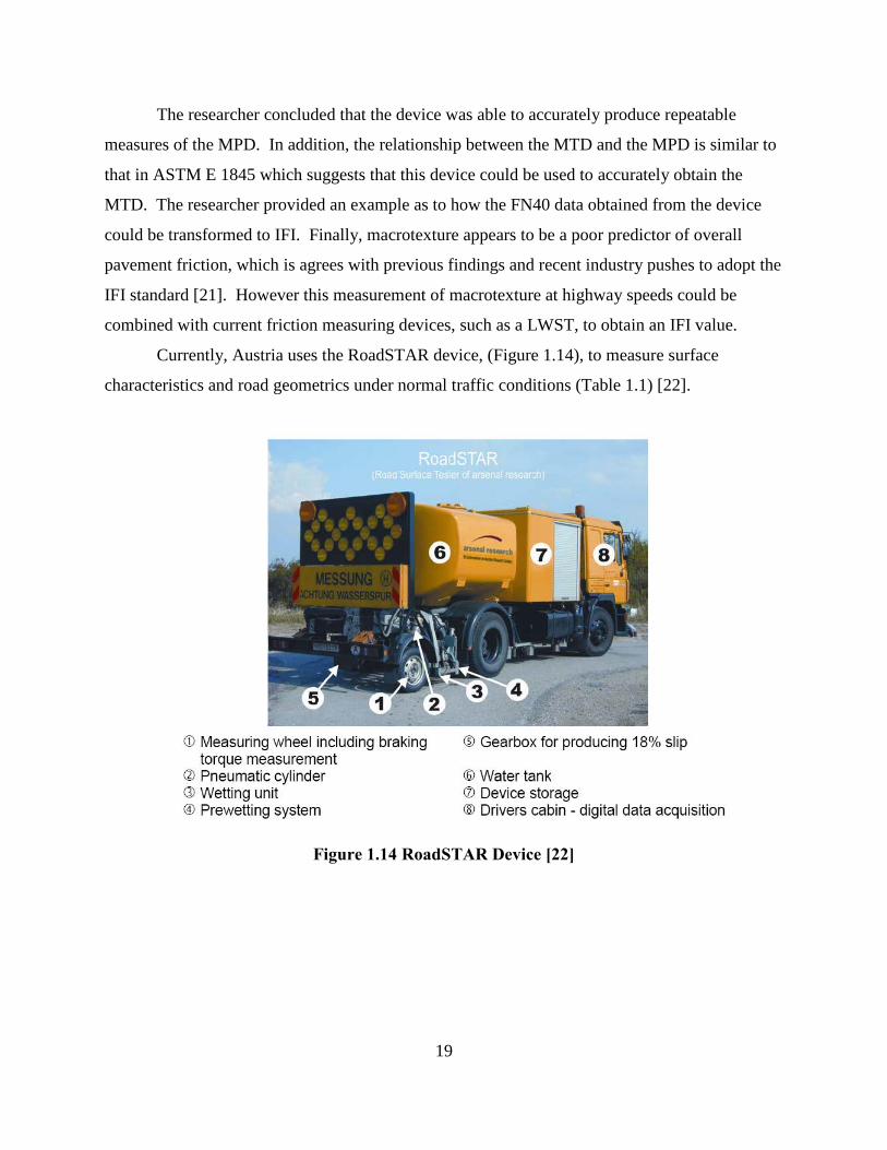
High Speed Laser Systems:
Recently Jackson [21] investigated the use of high-speed height-based sensor technology, as
shown in Figure 1.13, to obtain friction and surface characteristics of asphalt pavement surfaces.
Figure 1.13: FDOT Unit High-Speed Laser System [21].
19
The researcher concluded that the device was able to accurately produce repeatable
measures of the MPD. In addition, the relationship between the MTD and the MPD is similar to
that in ASTM E 1845 which suggests that this device could be used to accurately obtain the
MTD. The researcher provided an example as to how the FN40 data obtained from the device
could be transformed to IFI. Finally, macrotexture appears to be a poor predictor of overall
pavement friction, which is agrees with previous findings and recent industry pushes to adopt the
IFI standard [21]. However this measurement of macrotexture at highway speeds could be
combined with current friction measuring devices, such as a LWST, to obtain an IFI value.
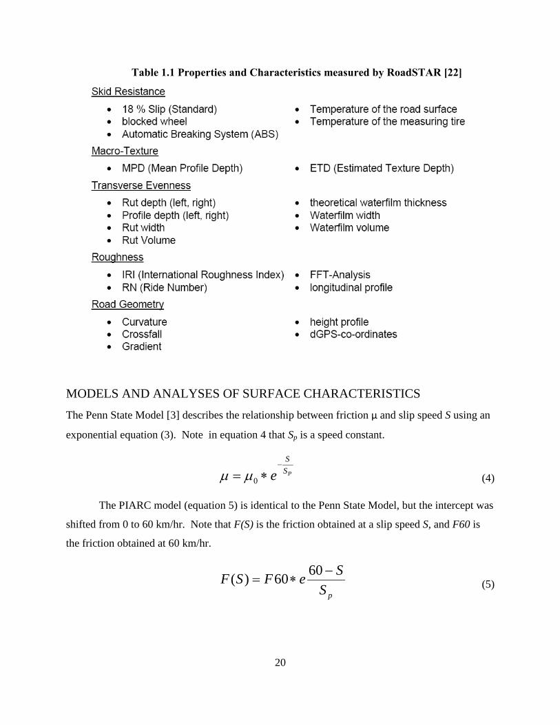
Currently, Austria uses the RoadSTAR device, (Figure 1.14), to measure surface
characteristics and road geometrics under normal traffic conditions (Table 1.1) [22].
Figure 1.14 RoadSTAR Device [22]
20
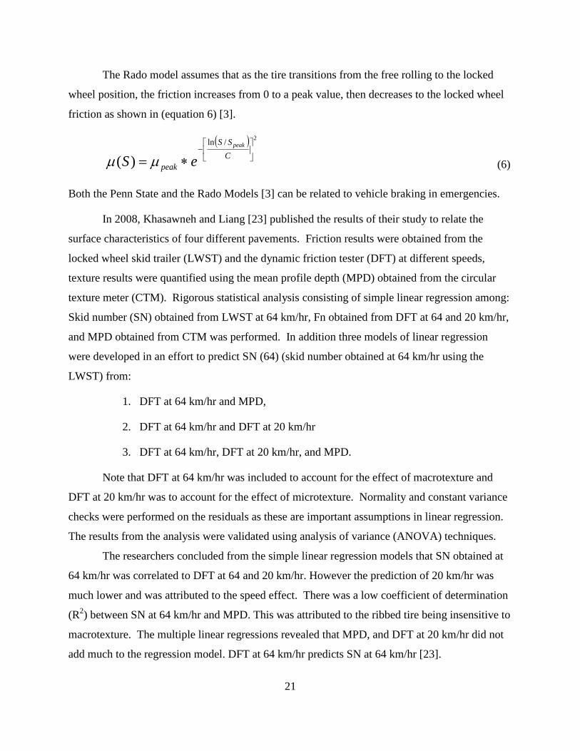
Table 1.1 Properties and Characteristics measured by RoadSTAR [22]
MODELS AND ANALYSES OF SURFACE CHARACTERISTICS The Penn State Model [3] describes the relationship between friction µ and slip speed S using an
exponential equation (3). Note in equation 4 that Sp is a speed constant.
PSS
e−
∗= 0µµ (4)
The PIARC model (equation 5) is identical to the Penn State Model, but the intercept was
shifted from 0 to 60 km/hr. Note that F(S) is the friction obtained at a slip speed S, and F60 is
the friction obtained at 60 km/hr.
pSSeFSF −
∗=6060)( (5)
21
The Rado model assumes that as the tire transitions from the free rolling to the locked
wheel position, the friction increases from 0 to a peak value, then decreases to the locked wheel
friction as shown in (equation 6) [3].
( ) 2/ln
)(
−
∗= CSS
peak
peak
eS µµ (6)
Both the Penn State and the Rado Models [3] can be related to vehicle braking in emergencies.
In 2008, Khasawneh and Liang [23] published the results of their study to relate the
surface characteristics of four different pavements. Friction results were obtained from the
locked wheel skid trailer (LWST) and the dynamic friction tester (DFT) at different speeds,
texture results were quantified using the mean profile depth (MPD) obtained from the circular
texture meter (CTM). Rigorous statistical analysis consisting of simple linear regression among:
Skid number (SN) obtained from LWST at 64 km/hr, Fn obtained from DFT at 64 and 20 km/hr,
and MPD obtained from CTM was performed. In addition three models of linear regression
were developed in an effort to predict SN (64) (skid number obtained at 64 km/hr using the
LWST) from:
1. DFT at 64 km/hr and MPD,
2. DFT at 64 km/hr and DFT at 20 km/hr
3. DFT at 64 km/hr, DFT at 20 km/hr, and MPD.
Note that DFT at 64 km/hr was included to account for the effect of macrotexture and
DFT at 20 km/hr was to account for the effect of microtexture. Normality and constant variance
checks were performed on the residuals as these are important assumptions in linear regression.
The results from the analysis were validated using analysis of variance (ANOVA) techniques.
The researchers concluded from the simple linear regression models that SN obtained at
64 km/hr was correlated to DFT at 64 and 20 km/hr. However the prediction of 20 km/hr was
much lower and was attributed to the speed effect. There was a low coefficient of determination
(R2) between SN at 64 km/hr and MPD. This was attributed to the ribbed tire being insensitive to
macrotexture. The multiple linear regressions revealed that MPD, and DFT at 20 km/hr did not
add much to the regression model. DFT at 64 km/hr predicts SN at 64 km/hr [23].
22
In 2000, Roo and Gerretsen [24] developed a simulation model (RODAS) to predict the
physical characteristics (texture, profile, porosity, specific flow resistance and acoustical
structure factor) from the HMA pavement material specifications of aggregate shape and
gradation, amount and type of binder, as well as the percentage of sand and filler. The RODAS
model was designed to be a module in the larger TRIAS (Tire Road Interaction Acoustical
Simulation) model to use road surface characteristics to aid in the design of quiet pavements.
They found that RODAS can predict the acoustical characteristics of pavement surfaces
with reasonable accuracy, the absorption model delivers a prediction inaccuracy (small enough
to distinguish different pavement types), and the texture prediction model needs to be improved
as it is not very accurate.
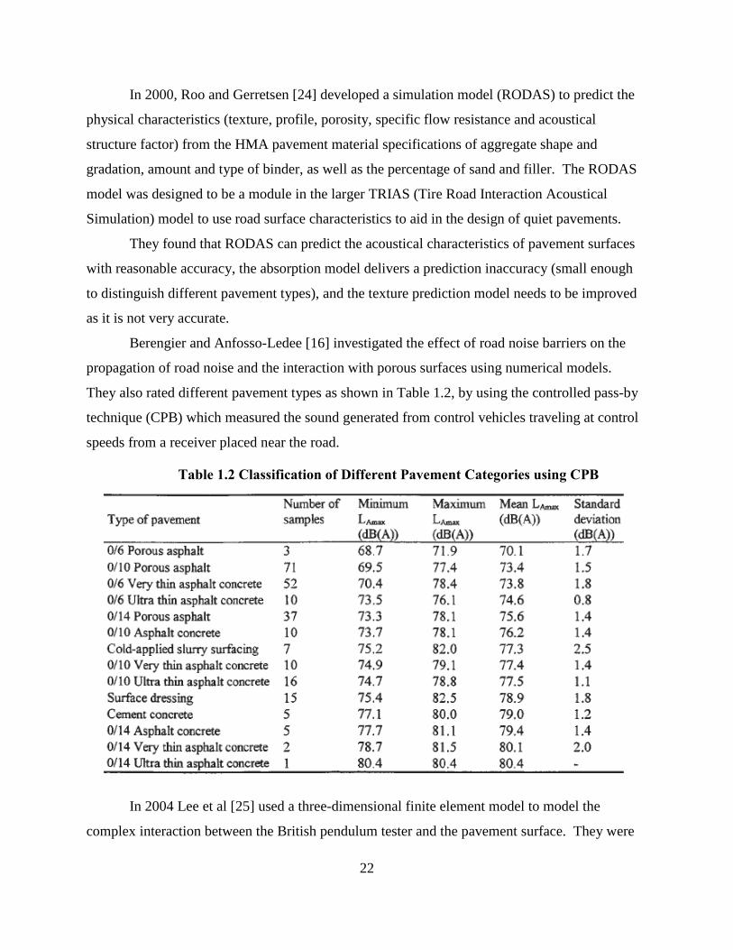
Berengier and Anfosso-Ledee [16] investigated the effect of road noise barriers on the
propagation of road noise and the interaction with porous surfaces using numerical models.
They also rated different pavement types as shown in Table 1.2, by using the controlled pass-by
technique (CPB) which measured the sound generated from control vehicles traveling at control
speeds from a receiver placed near the road.
Table 1.2 Classification of Different Pavement Categories using CPB
In 2004 Lee et al [25] used a three-dimensional finite element model to model the
complex interaction between the British pendulum tester and the pavement surface. They were

23
able to obtain to obtain a skid resistance value and other contact information based on the surface
type without having to perform the physical test.
Trifiro et al [26] analyzed different pavement sections at the Virginia Smart Road by
measuring the friction with different devices, at different speeds and obtaining an international
friction index value, IFI, as defined by PIRAC. The researchers found that the repeatability of
the locked wheel skid trailers (LWST) was good, as were LWST tests of using the same tire at
different speeds. However the ribbed tire did not correlate with the smooth tire, and there were
discrepancies among the IFI values calculated using the different devices.
McGhee et al [27] performed continuous texture measurements using laser-based devices
as a possible tool to aid in detecting segregation and non-uniformity of HMA mixtures. The
researchers concluded that the method “holds great promise”.
NCHRP Web Document No. 42 [15] presented the issues related to pavement
smoothness and highlighted the main concerns related to pavement smoothness including:
• Accuracy and repeatability of equipment
• Reproducibility of equipment
• Use of profile data for corrective action
• Knowledge and understanding of equipment and measures
• Relating smoothness to cost and performance
• Identifying and appropriate index for smoothness
• Lack of standard guide specifications
• Future use of profile data
• Using smoothness index to monitor pavement performance
24
INTERRELATIONSHIPS AMONG SURFACE CHARACTERISTICS National Cooperative Highway Research Program (NCHRP) Synthesis No. 291 [3] reviewed the
current state of the art for measuring and characterizing pavement surface characteristics by
surveying national and international agencies and by conducting a literature review. The report
noted the following relationships between pavement design parameters and surface
characteristics:
• Splash and spray was reduced and skid resistance improved with an increase in
macrotexture, especially porous pavements.
• Exterior noise levels increase with increasing macrotexture, however the range of
macrotexture also influences the skid resistance.
• In vehicle noise was affected by higher wavelengths of macrotexture and megatexture.
• The relationship between tire wear and microtexture was not deemed important by
agencies, and no models could be found in literature
The report also commented on the surface characteristics of the following asphalt surfaces and
maintenance treatments.
• Stone Mastic Asphalt (SMA) pavements tend to have great macrotexture properties and
the ability retain these properties under heavy truck traffic
• Superpave pavements are designed to combat rutting which reduces the tendency to
hydroplane, there is no consideration given to surface texture or skid resistance.
• Microsurfacing Treatments are durable treatments that restore macrotexture treatments
and to some degree, ride quality to asphalt pavements; many proprietary products have
been applied in Europe and the U.S.
• Seal Coats typically provide similar macrotexture benefits as Microsurfacing treatments,
but use more conventional materials.
FRICTION & HMA DESIGN PARAMETERS
Flintsch et al [45] recently investigated the relationship between the International Friction Index
(IFI), HMA design characteristics, and certain testing conditions at the Virginia Smart Road.
The different HMA mixes studied included five different Superpave mixes, a stone mastic
asphalt (SMA) and an open graded friction course (OGFC). The surface characteristics were
25
measured using an LWST, a British Pendulum Tester and laser texture devices while considering
the test tire, the vehicle test speed, and the grade.
The researchers found that the friction measurements were dependent upon texture, age
and temperature. They noted that past studies demonstrated that “aggregate type and structure
significantly influence microtexture and macrotexture, thus influencing the skid resistance of a
paved surface (Henry and Dahir, 1979; Forster, 1989; Kandhal and Frazier, 1998)”. They
investigated the effect of the HMA design parameters of speed constant (Sp) and the normalized
friction value (F60) of IFI using a stepwise regression analysis. The results of the analysis
(shown below) indicate that SP can be predicted from NMS and VMA, and that friction increases
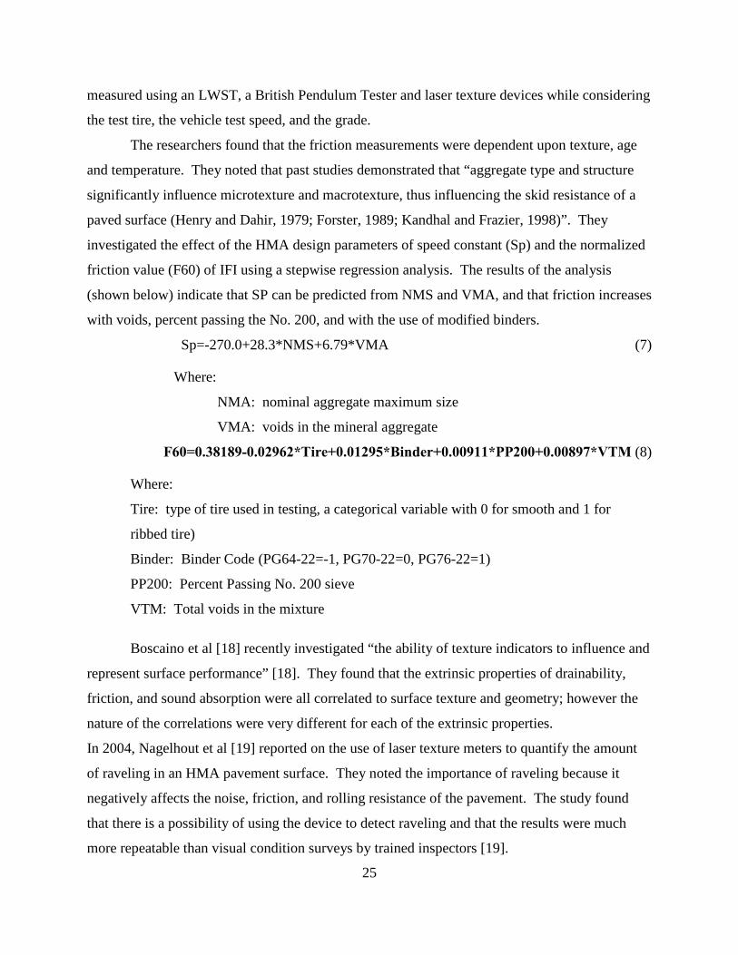
with voids, percent passing the No. 200, and with the use of modified binders.
Sp=-270.0+28.3*NMS+6.79*VMA (7)
Where:
NMA: nominal aggregate maximum size
VMA: voids in the mineral aggregate
F60=0.38189-0.02962*Tire+0.01295*Binder+0.00911*PP200+0.00897*VTM (8)
Where:
Tire: type of tire used in testing, a categorical variable with 0 for smooth and 1 for
ribbed tire)
Binder: Binder Code (PG64-22=-1, PG70-22=0, PG76-22=1)
PP200: Percent Passing No. 200 sieve
VTM: Total voids in the mixture
Boscaino et al [18] recently investigated “the ability of texture indicators to influence and
represent surface performance” [18]. They found that the extrinsic properties of drainability,
friction, and sound absorption were all correlated to surface texture and geometry; however the
nature of the correlations were very different for each of the extrinsic properties.
In 2004, Nagelhout et al [19] reported on the use of laser texture meters to quantify the amount
of raveling in an HMA pavement surface. They noted the importance of raveling because it
negatively affects the noise, friction, and rolling resistance of the pavement. The study found
that there is a possibility of using the device to detect raveling and that the results were much
more repeatable than visual condition surveys by trained inspectors [19].
26
TEXTURE & NOISE
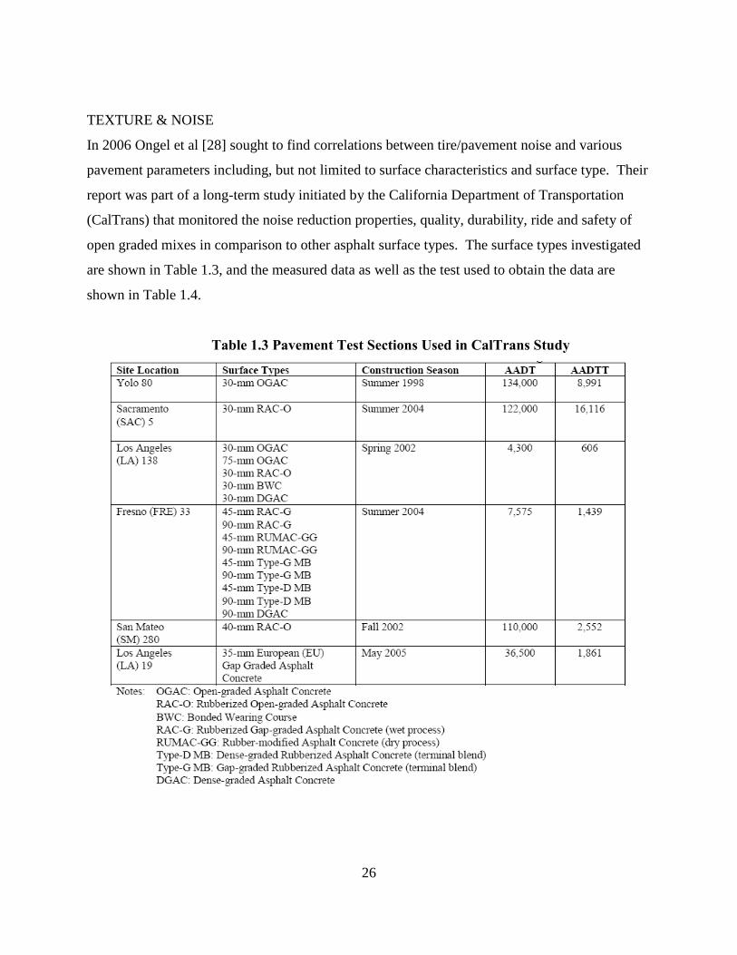
In 2006 Ongel et al [28] sought to find correlations between tire/pavement noise and various
pavement parameters including, but not limited to surface characteristics and surface type. Their
report was part of a long-term study initiated by the California Department of Transportation
(CalTrans) that monitored the noise reduction properties, quality, durability, ride and safety of
open graded mixes in comparison to other asphalt surface types. The surface types investigated
are shown in Table 1.3, and the measured data as well as the test used to obtain the data are
shown in Table 1.4.
Table 1.3 Pavement Test Sections Used in CalTrans Study
27
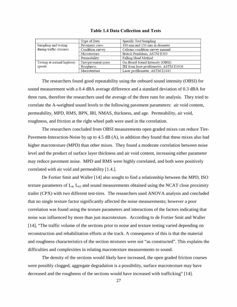
Table 1.4 Data Collection and Tests
The researchers found good repeatability using the onboard sound intensity (OBSI) for
sound measurement with a 0.4 dBA average difference and a standard deviation of 0.3 dBA for
three runs, therefore the researchers used the average of the three runs for analysis. They tried to
correlate the A-weighted sound levels to the following pavement parameters: air void content,
permeability, MPD, RMS, BPN, IRI, NMAS, thickness, and age. Permeability, air void,
roughness, and friction at the right wheel path were used in the correlation.
The researchers concluded from OBSI measurements open graded mixes can reduce Tire-
Pavement-Interaction-Noise by up to 4.5 dB (A), in addition they found that these mixes also had
higher macrotexture (MPD) than other mixes. They found a moderate correlation between noise
level and the product of surface layer thickness and air void content, increasing either parameter
may reduce pavement noise. MPD and RMS were highly correlated, and both were positively
correlated with air void and permeability [1.4.].
De Fortier Smit and Waller [14] also sought to find a relationship between the MPD, ISO
texture parameters of L4, L63 and sound measurements obtained using the NCAT close proximity
trailer (CPX) with two different test-tires. The researchers used ANOVA analysis and concluded
that no single texture factor significantly affected the noise measurements; however a poor
correlation was found using the texture parameters and interactions of the factors indicating that
noise was influenced by more than just macrotexture. According to de Fortier Smit and Waller
[14], “The traffic volume of the sections prior to noise and texture testing varied depending on
reconstruction and rehabilitation efforts at the track. A consequence of this is that the material
and roughness characteristics of the section mixtures were not “as constructed”. This explains the
difficulties and complexities in relating macrotexture measurements to sound.
The density of the sections would likely have increased, the open graded friction courses
were possibly clogged, aggregate degradation is a possibility, surface macrotexture may have
decreased and the roughness of the sections would have increased with trafficking” [14].

28
The researchers also suggested warming the test tires for at least twenty minutes prior to testing
to ensure test repeatability in sound pressure measurements.
CHAPTER CONCLUDING REMARKS Many different methods can be used to characterize the pavement’s several interrelated
surface characteristics. These surface characteristics are affected by not only short term and long
term seasonal and temperature effects, but also are dependent upon the device being used. This
necessitates the frequent testing of sections and calibration of equipment and further complicates
correlation of measured results with other devices. Recent advances in laser technology and
computing are improving the ease, frequency and repeatability with which measurements can be
taken, especially in facilitating the analysis of the spectral content of the surface characteristics.
Many pavement practitioners have expressed interest in IFI which is hoped to harmonize
friction measurements by incorporating both a macrotexture and a normalized friction
measurement into the value. This would make it easier to compare results obtained from
different devices and accurately characterize the pavement’s surface.
There has been limited success in relating different pavement surface characteristics with design
parameters in an attempt to optimize properties and better characterize behavior. Often times
optimizing one characteristic such as friction causes an increase in another characteristic such as
noise; however porous pavements have good macrotexture qualities and absorb sound relatively
well when compared with other HMA pavement types.
Literature shows that there may be predictive models relating asphalt surface properties.
This underscores the need to perform, data analysis to ascertain if some correlation trends may
exist or if some of those postulated are valid. However, they are susceptible to “ drain down” and
raveling.

29
CHAPTER 2
CONSTRUCTION AND INITIAL TESTING OF VARIOUS TEST
CELLS
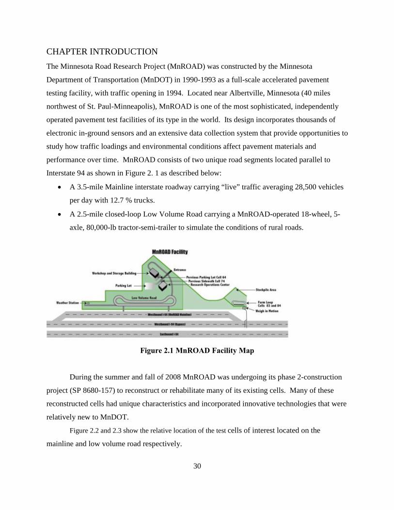
30
CHAPTER INTRODUCTION The Minnesota Road Research Project (MnROAD) was constructed by the Minnesota
Department of Transportation (MnDOT) in 1990-1993 as a full-scale accelerated pavement
testing facility, with traffic opening in 1994. Located near Albertville, Minnesota (40 miles
northwest of St. Paul-Minneapolis), MnROAD is one of the most sophisticated, independently
operated pavement test facilities of its type in the world. Its design incorporates thousands of
electronic in-ground sensors and an extensive data collection system that provide opportunities to
study how traffic loadings and environmental conditions affect pavement materials and
performance over time. MnROAD consists of two unique road segments located parallel to
Interstate 94 as shown in Figure 2. 1 as described below:
• A 3.5-mile Mainline interstate roadway carrying “live” traffic averaging 28,500 vehicles
per day with 12.7 % trucks.
• A 2.5-mile closed-loop Low Volume Road carrying a MnROAD-operated 18-wheel, 5-
axle, 80,000-lb tractor-semi-trailer to simulate the conditions of rural roads.
Figure 2.1 MnROAD Facility Map
During the summer and fall of 2008 MnROAD was undergoing its phase 2-construction
project (SP 8680-157) to reconstruct or rehabilitate many of its existing cells. Many of these
reconstructed cells had unique characteristics and incorporated innovative technologies that were
relatively new to MnDOT.
Figure 2.2 and 2.3 show the relative location of the test cells of interest located on the
mainline and low volume road respectively.
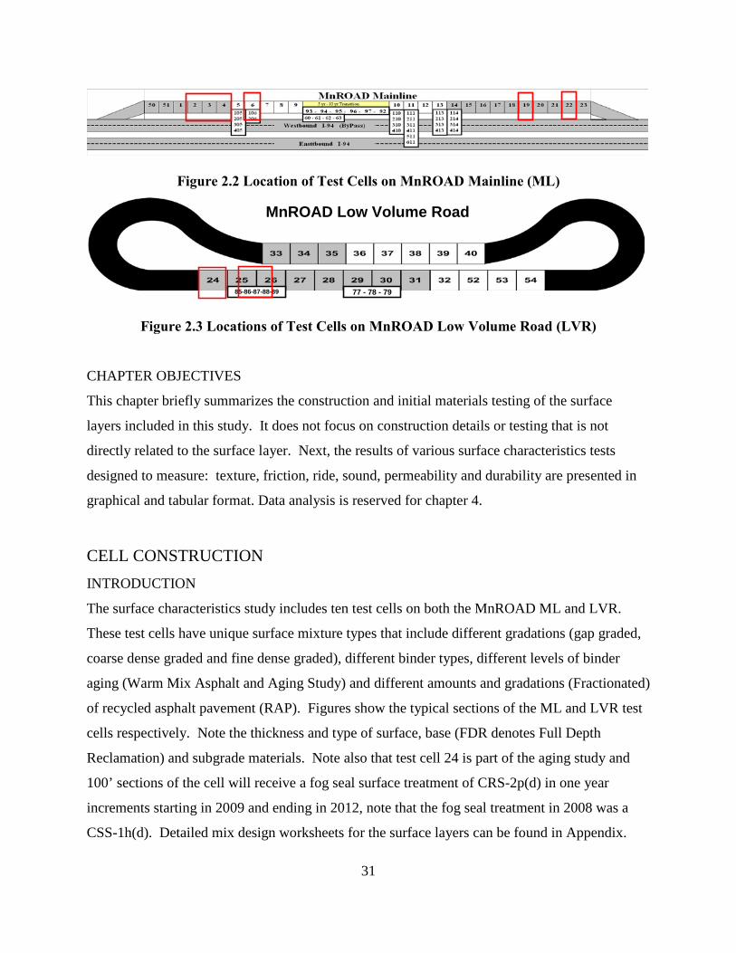
31
Figure 2.2 Location of Test Cells on MnROAD Mainline (ML)
Figure 2.3 Locations of Test Cells on MnROAD Low Volume Road (LVR)
85-86-87-88-89 77 - 78 - 79
MnROAD Low Volume Road
CHAPTER OBJECTIVES
This chapter briefly summarizes the construction and initial materials testing of the surface
layers included in this study. It does not focus on construction details or testing that is not
directly related to the surface layer. Next, the results of various surface characteristics tests
designed to measure: texture, friction, ride, sound, permeability and durability are presented in
graphical and tabular format. Data analysis is reserved for chapter 4.
CELL CONSTRUCTION INTRODUCTION
The surface characteristics study includes ten test cells on both the MnROAD ML and LVR.
These test cells have unique surface mixture types that include different gradations (gap graded,
coarse dense graded and fine dense graded), different binder types, different levels of binder
aging (Warm Mix Asphalt and Aging Study) and different amounts and gradations (Fractionated)
of recycled asphalt pavement (RAP). Figures show the typical sections of the ML and LVR test
cells respectively. Note the thickness and type of surface, base (FDR denotes Full Depth
Reclamation) and subgrade materials. Note also that test cell 24 is part of the aging study and
100’ sections of the cell will receive a fog seal surface treatment of CRS-2p(d) in one year
increments starting in 2009 and ending in 2012, note that the fog seal treatment in 2008 was a
CSS-1h(d). Detailed mix design worksheets for the surface layers can be found in Appendix.
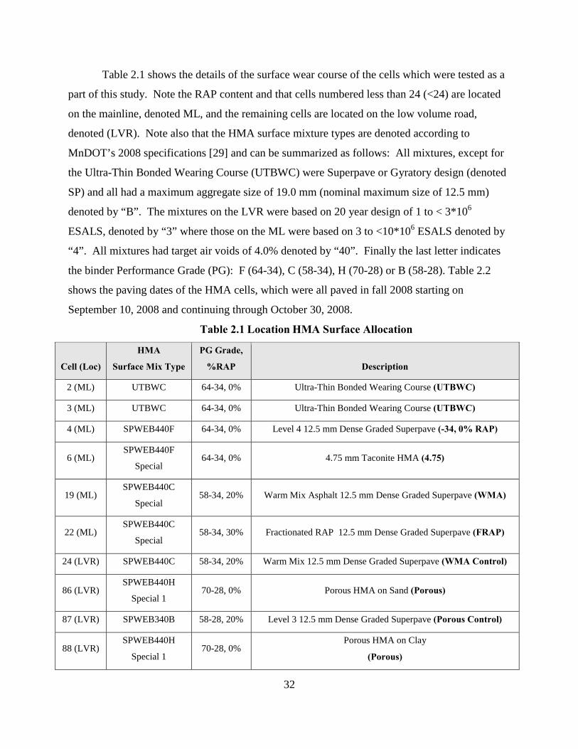
32
Table 2.1 shows the details of the surface wear course of the cells which were tested as a
part of this study. Note the RAP content and that cells numbered less than 24 (<24) are located
on the mainline, denoted ML, and the remaining cells are located on the low volume road,
denoted (LVR). Note also that the HMA surface mixture types are denoted according to
MnDOT’s 2008 specifications [29] and can be summarized as follows: All mixtures, except for
the Ultra-Thin Bonded Wearing Course (UTBWC) were Superpave or Gyratory design (denoted
SP) and all had a maximum aggregate size of 19.0 mm (nominal maximum size of 12.5 mm)
denoted by “B”. The mixtures on the LVR were based on 20 year design of 1 to < 3*106
ESALS, denoted by “3” where those on the ML were based on 3 to <10*106 ESALS denoted by
“4”. All mixtures had target air voids of 4.0% denoted by “40”. Finally the last letter indicates
the binder Performance Grade (PG): F (64-34), C (58-34), H (70-28) or B (58-28). Table 2.2
shows the paving dates of the HMA cells, which were all paved in fall 2008 starting on
September 10, 2008 and continuing through October 30, 2008.
Table 2.1 Location HMA Surface Allocation
Cell (Loc)
HMA
Surface Mix Type
PG Grade,
%RAP Description
2 (ML) UTBWC 64-34, 0% Ultra-Thin Bonded Wearing Course (UTBWC)
3 (ML) UTBWC 64-34, 0% Ultra-Thin Bonded Wearing Course (UTBWC)
4 (ML) SPWEB440F 64-34, 0% Level 4 12.5 mm Dense Graded Superpave (-34, 0% RAP)
6 (ML) SPWEB440F
Special 64-34, 0% 4.75 mm Taconite HMA (4.75)
19 (ML) SPWEB440C
Special 58-34, 20% Warm Mix Asphalt 12.5 mm Dense Graded Superpave (WMA)
22 (ML) SPWEB440C
Special 58-34, 30% Fractionated RAP 12.5 mm Dense Graded Superpave (FRAP)
24 (LVR) SPWEB440C 58-34, 20% Warm Mix 12.5 mm Dense Graded Superpave (WMA Control)
86 (LVR) SPWEB440H
Special 1 70-28, 0% Porous HMA on Sand (Porous)
87 (LVR) SPWEB340B 58-28, 20% Level 3 12.5 mm Dense Graded Superpave (Porous Control)
88 (LVR) SPWEB440H
Special 1 70-28, 0%
Porous HMA on Clay
(Porous)
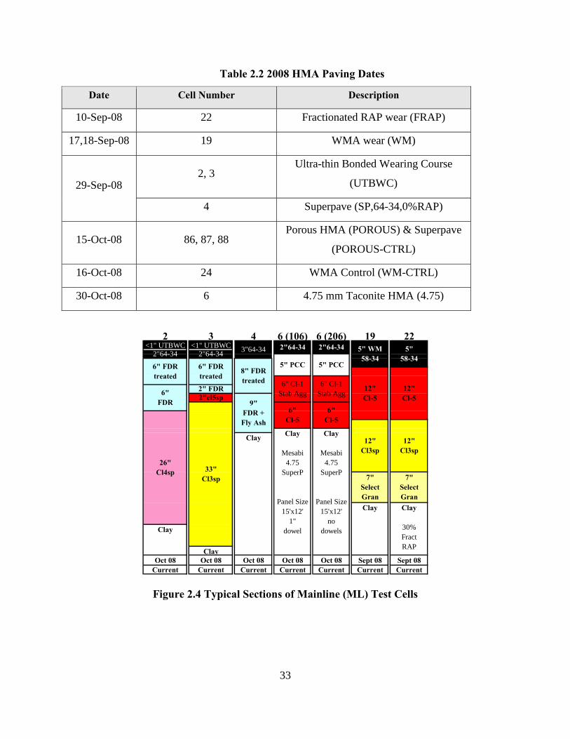
33
Table 2.2 2008 HMA Paving Dates
Date Cell Number Description
10-Sep-08 22 Fractionated RAP wear (FRAP)
17,18-Sep-08 19 WMA wear (WM)
29-Sep-08 2, 3
Ultra-thin Bonded Wearing Course
(UTBWC)
4 Superpave (SP,64-34,0%RAP)
15-Oct-08 86, 87, 88 Porous HMA (POROUS) & Superpave
(POROUS-CTRL)
16-Oct-08 24 WMA Control (WM-CTRL)
30-Oct-08 6 4.75 mm Taconite HMA (4.75)
Figure 2.4 Typical Sections of Mainline (ML) Test Cells
2 3 4 6 (106) 6 (206) 19 22<1" UTBWC <1" UTBWC
Oct 08 Oct 08 Oct 08 Oct 08 Oct 08 Sept 08 Sept 08Current Current Current Current Current Current Current
5"58-34
12"Cl-5
12"Cl3sp
7"SelectGran
Clay
Mesabi4.75
SuperP
Panel Size 15'x12'
1"dowel
Clay
Mesabi4.75
SuperP
Panel Size 15'x12'
nodowels
5" WM58-34
12"Cl-5
12"Cl3sp
7"SelectGranClay Clay
30%FractRAPClay
Clay
26"Cl4sp
2" FDR6"FDR
6" FDRtreated
33"Cl3sp
8" FDRtreated
2"64-34
2"cl5sp
6" FDRtreated
2"64-34
9" FDR +Fly Ash
3"64-34 2"64-34 2"64-34
5" PCC
Clay
5" PCC
6" Cl-1Stab Agg
6" Cl-1Stab Agg
6"Cl-5
6"Cl-5
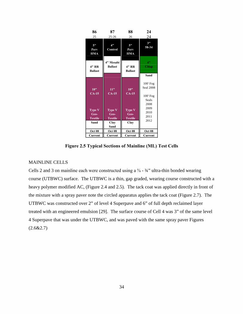
34
Figure 2.5 Typical Sections of Mainline (ML) Test Cells
86 87 88 2425 25-26 26 24
Oct 08 Oct 08 Oct 08 Oct 08Current Current Current Current
3"58-34
4"Cl6sp
Sand
100' Fog Seal 2008
100' Fog Seals 20082009201020112012
4"Control
Clay
4" RRBallast
4" MesabiBallast 4" RR
Ballast
5"PervHMA
5"PervHMA
Sand ClaySand
10"CA-15
Type VGeo-
Textile
11"CA-15
Type VGeo-
Textile
10"CA-15
Type VGeo-
Textile
MAINLINE CELLS
Cells 2 and 3 on mainline each were constructed using a ⅝ - ¾” ultra-thin bonded wearing
course (UTBWC) surface. The UTBWC is a thin, gap graded, wearing course constructed with a
heavy polymer modified AC, (Figure 2.4 and 2.5). The tack coat was applied directly in front of
the mixture with a spray paver note the circled apparatus applies the tack coat (Figure 2.7). The
UTBWC was constructed over 2” of level 4 Superpave and 6” of full depth reclaimed layer
treated with an engineered emulsion [29]. The surface course of Cell 4 was 3” of the same level
4 Superpave that was under the UTBWC, and was paved with the same spray paver Figures
(2.6&2.7)
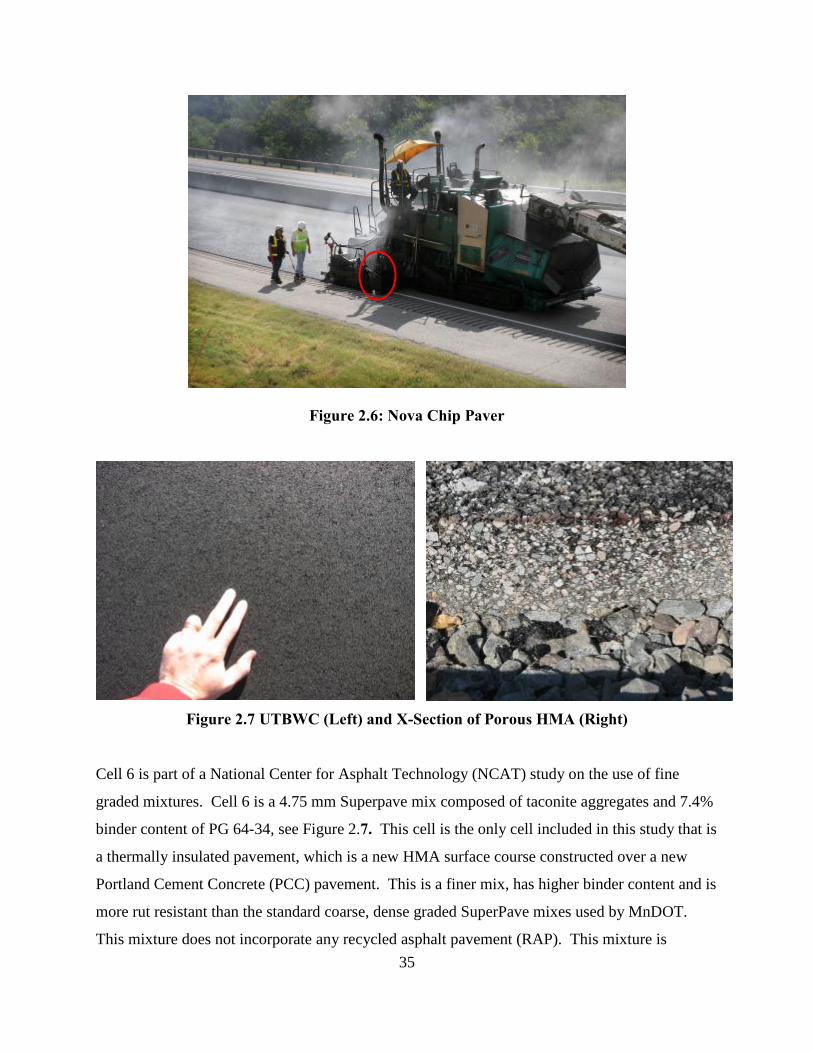
35
Figure 2.6: Nova Chip Paver
Figure 2.7 UTBWC (Left) and X-Section of Porous HMA (Right)
Cell 6 is part of a National Center for Asphalt Technology (NCAT) study on the use of fine
graded mixtures. Cell 6 is a 4.75 mm Superpave mix composed of taconite aggregates and 7.4%
binder content of PG 64-34, see Figure 2.7. This cell is the only cell included in this study that is
a thermally insulated pavement, which is a new HMA surface course constructed over a new
Portland Cement Concrete (PCC) pavement. This is a finer mix, has higher binder content and is
more rut resistant than the standard coarse, dense graded SuperPave mixes used by MnDOT.
This mixture does not incorporate any recycled asphalt pavement (RAP). This mixture is
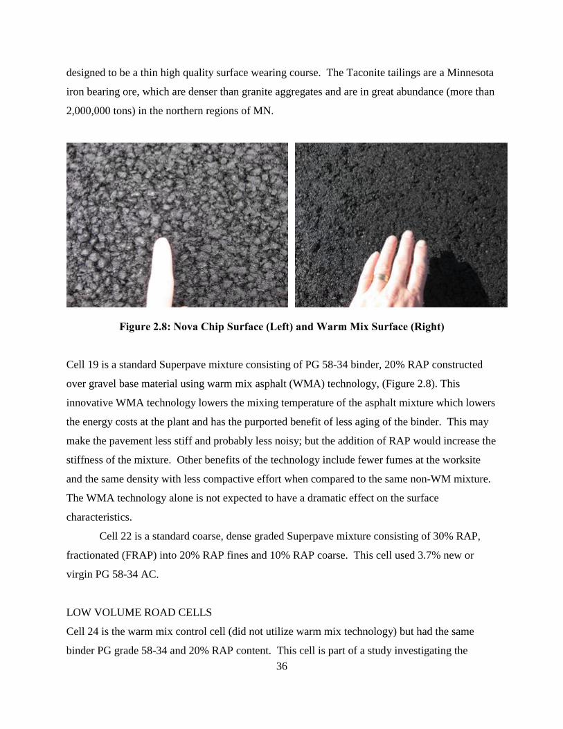
36
designed to be a thin high quality surface wearing course. The Taconite tailings are a Minnesota
iron bearing ore, which are denser than granite aggregates and are in great abundance (more than
2,000,000 tons) in the northern regions of MN.
Figure 2.8: Nova Chip Surface (Left) and Warm Mix Surface (Right)
Cell 19 is a standard Superpave mixture consisting of PG 58-34 binder, 20% RAP constructed
over gravel base material using warm mix asphalt (WMA) technology, (Figure 2.8). This
innovative WMA technology lowers the mixing temperature of the asphalt mixture which lowers
the energy costs at the plant and has the purported benefit of less aging of the binder. This may
make the pavement less stiff and probably less noisy; but the addition of RAP would increase the
stiffness of the mixture. Other benefits of the technology include fewer fumes at the worksite
and the same density with less compactive effort when compared to the same non-WM mixture.
The WMA technology alone is not expected to have a dramatic effect on the surface
characteristics.
Cell 22 is a standard coarse, dense graded Superpave mixture consisting of 30% RAP,
fractionated (FRAP) into 20% RAP fines and 10% RAP coarse. This cell used 3.7% new or
virgin PG 58-34 AC.
LOW VOLUME ROAD CELLS
Cell 24 is the warm mix control cell (did not utilize warm mix technology) but had the same
binder PG grade 58-34 and 20% RAP content. This cell is part of a study investigating the
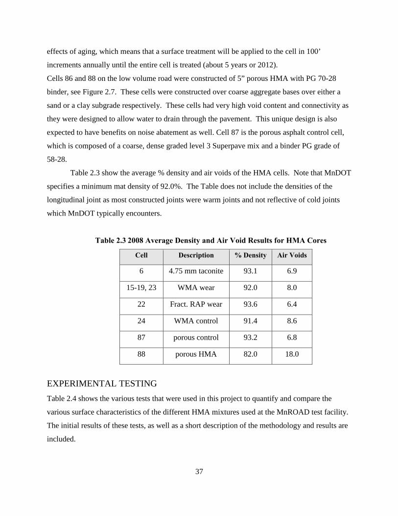
37
effects of aging, which means that a surface treatment will be applied to the cell in 100’
increments annually until the entire cell is treated (about 5 years or 2012).
Cells 86 and 88 on the low volume road were constructed of 5” porous HMA with PG 70-28
binder, see Figure 2.7. These cells were constructed over coarse aggregate bases over either a
sand or a clay subgrade respectively. These cells had very high void content and connectivity as
they were designed to allow water to drain through the pavement. This unique design is also
expected to have benefits on noise abatement as well. Cell 87 is the porous asphalt control cell,
which is composed of a coarse, dense graded level 3 Superpave mix and a binder PG grade of
58-28.
Table 2.3 show the average % density and air voids of the HMA cells. Note that MnDOT
specifies a minimum mat density of 92.0%. The Table does not include the densities of the
longitudinal joint as most constructed joints were warm joints and not reflective of cold joints
which MnDOT typically encounters.
Table 2.3 2008 Average Density and Air Void Results for HMA Cores
Cell Description % Density Air Voids
6 4.75 mm taconite 93.1 6.9
15-19, 23 WMA wear 92.0 8.0
22 Fract. RAP wear 93.6 6.4
24 WMA control 91.4 8.6
87 porous control 93.2 6.8
88 porous HMA 82.0 18.0
EXPERIMENTAL TESTING Table 2.4 shows the various tests that were used in this project to quantify and compare the
various surface characteristics of the different HMA mixtures used at the MnROAD test facility.
The initial results of these tests, as well as a short description of the methodology and results are
included.
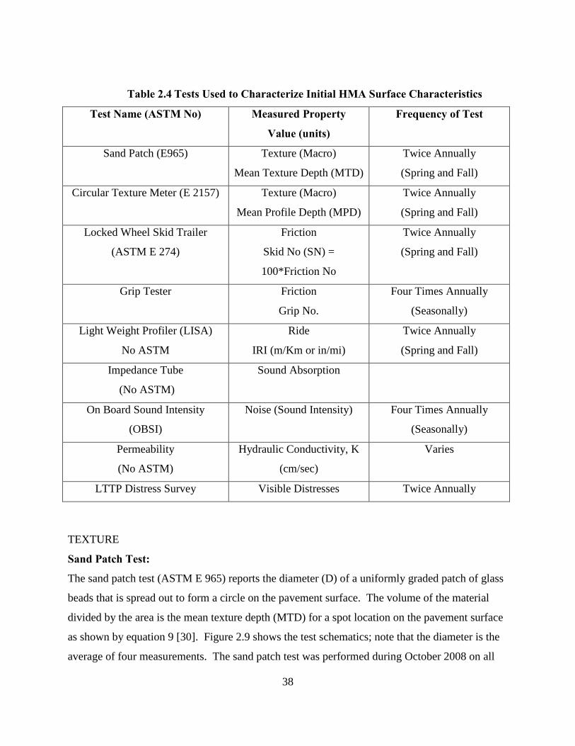
38
Table 2.4 Tests Used to Characterize Initial HMA Surface Characteristics
Test Name (ASTM No) Measured Property
Value (units)
Frequency of Test
Sand Patch (E965) Texture (Macro)
Mean Texture Depth (MTD)
Twice Annually
(Spring and Fall)
Circular Texture Meter (E 2157) Texture (Macro)
Mean Profile Depth (MPD)
Twice Annually
(Spring and Fall)
Locked Wheel Skid Trailer
(ASTM E 274)
Friction
Skid No (SN) =
100*Friction No
Twice Annually
(Spring and Fall)
Grip Tester Friction
Grip No.
Four Times Annually
(Seasonally)
Light Weight Profiler (LISA)
No ASTM
Ride
IRI (m/Km or in/mi)
Twice Annually
(Spring and Fall)
Impedance Tube
(No ASTM)
Sound Absorption
On Board Sound Intensity
(OBSI)
Noise (Sound Intensity) Four Times Annually
(Seasonally)
Permeability
(No ASTM)
Hydraulic Conductivity, K
(cm/sec)
Varies
LTTP Distress Survey Visible Distresses Twice Annually
TEXTURE Sand Patch Test:
The sand patch test (ASTM E 965) reports the diameter (D) of a uniformly graded patch of glass
beads that is spread out to form a circle on the pavement surface. The volume of the material
divided by the area is the mean texture depth (MTD) for a spot location on the pavement surface
as shown by equation 9 [30]. Figure 2.9 shows the test schematics; note that the diameter is the
average of four measurements. The sand patch test was performed during October 2008 on all
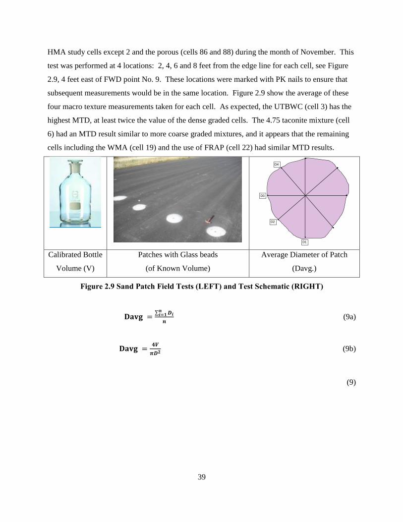
39
HMA study cells except 2 and the porous (cells 86 and 88) during the month of November. This
test was performed at 4 locations: 2, 4, 6 and 8 feet from the edge line for each cell, see Figure
2.9, 4 feet east of FWD point No. 9. These locations were marked with PK nails to ensure that
subsequent measurements would be in the same location. Figure 2.9 show the average of these
four macro texture measurements taken for each cell. As expected, the UTBWC (cell 3) has the
highest MTD, at least twice the value of the dense graded cells. The 4.75 taconite mixture (cell
6) had an MTD result similar to more coarse graded mixtures, and it appears that the remaining
cells including the WMA (cell 19) and the use of FRAP (cell 22) had similar MTD results.
Figure 2.9 Sand Patch Field Tests (LEFT) and Test Schematic (RIGHT)
𝐃𝐚𝐯𝐠 = ∑ 𝑫𝒊𝒏𝒊=𝟏𝒏
Calibrated Bottle
Volume (V)
Patches with Glass beads
(of Known Volume)
Average Diameter of Patch
(Davg.)
D1
D2
D3
D4
(9a)
𝐃𝐚𝐯𝐠 = 𝟒𝑽𝝅𝑫𝟐
(9b)
(9)
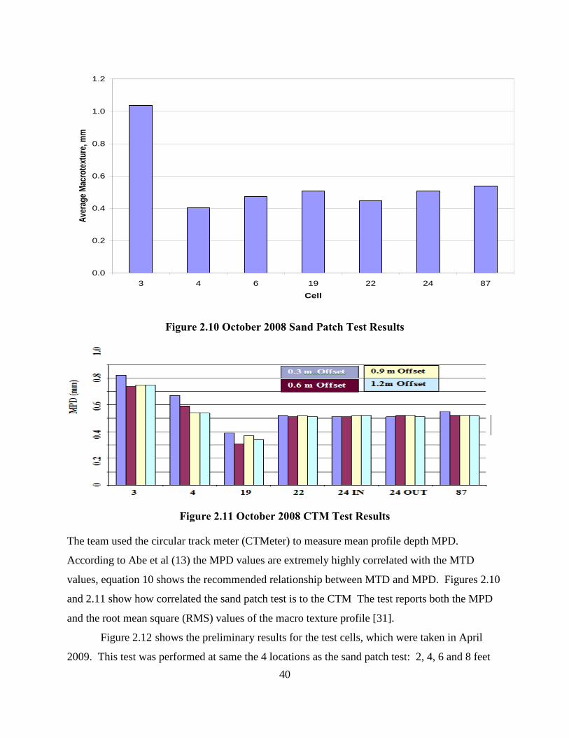
40
Figure 2.10 October 2008 Sand Patch Test Results
0.0
0.2
0.4
0.6
0.8
1.0
1.2
3 4 6 19 22 24 87
Cell
Aver
age M
acro
textu
re, m
m
Figure 2.11 October 2008 CTM Test Results
The team used the circular track meter (CTMeter) to measure mean profile depth MPD.
According to Abe et al (13) the MPD values are extremely highly correlated with the MTD
values, equation 10 shows the recommended relationship between MTD and MPD. Figures 2.10
and 2.11 show how correlated the sand patch test is to the CTM The test reports both the MPD
and the root mean square (RMS) values of the macro texture profile [31].
Figure 2.12 shows the preliminary results for the test cells, which were taken in April
2009. This test was performed at same the 4 locations as the sand patch test: 2, 4, 6 and 8 feet
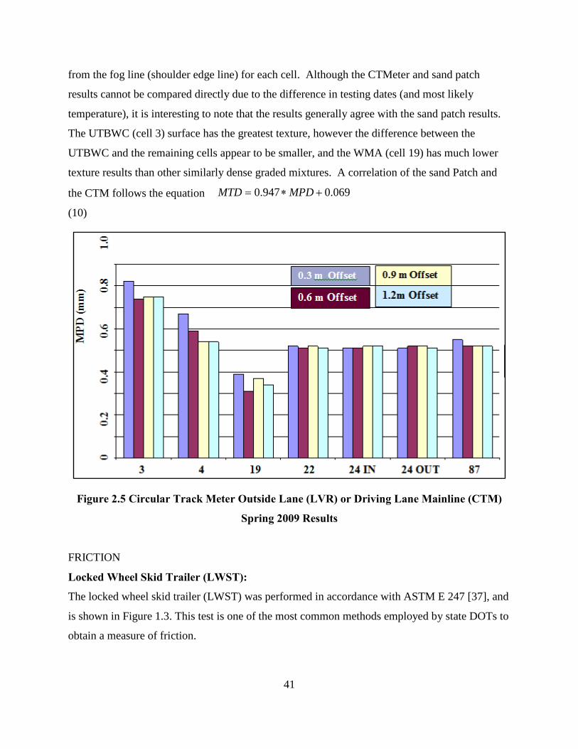
41
from the fog line (shoulder edge line) for each cell. Although the CTMeter and sand patch
results cannot be compared directly due to the difference in testing dates (and most likely
temperature), it is interesting to note that the results generally agree with the sand patch results.
The UTBWC (cell 3) surface has the greatest texture, however the difference between the
UTBWC and the remaining cells appear to be smaller, and the WMA (cell 19) has much lower
texture results than other similarly dense graded mixtures. A correlation of the sand Patch and
the CTM follows the equation
(10)
069.0947.0 +∗= MPDMTD
Figure 2.5 Circular Track Meter Outside Lane (LVR) or Driving Lane Mainline (CTM)
Spring 2009 Results
FRICTION
Locked Wheel Skid Trailer (LWST): The locked wheel skid trailer (LWST) was performed in accordance with ASTM E 247 [37], and
is shown in Figure 1.3. This test is one of the most common methods employed by state DOTs to
obtain a measure of friction.
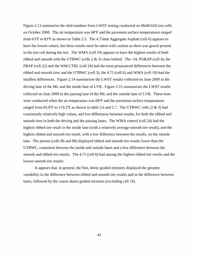
42
Figure 2.13 summarize the skid numbers from LWST testing conducted on MnROAD test cells
on October 2008. The air temperature was 68ºF and the pavement surface temperatures ranged
from 63ºF to 83ºF as shown in Table 2.5. The 4.75mm Aggregate Asphalt (cell 6) appears to
have the lowest values, but these results must be taken with caution as there was gravel present
in the test cell during the test. The WMA (cell 19) appears to have the highest results of both
ribbed and smooth with the UTBWC (cells 2 & 3) close behind. The -34, 0%RAP (cell 4), the
FRAP (cell 22) and the WM-CTRL (cell 24) had the most pronounced differences between the
ribbed and smooth tires and the UTBWC (cell 3), the 4.75 (cell 6) and WMA (cell 19) had the
smallest differences. Figure 2.14 summarizes the LWST results collected on June 2009 in the
driving lane of the ML and the inside lane of LVR. Figure 2.15 summarizes the LWST results
collected on June 2009 in the passing lane of the ML and the outside lane of LVR. These tests
were conducted when the air temperature was 68ºF and the pavement surface temperatures
ranged from 85.8ºF to 119.2ºF as shown in table 2.6 and 2.7. The UTBWC cells (2 & 3) had
consistently relatively high values, and low differences between results, for both the ribbed and
smooth tires in both the driving and the passing lanes. The WMA control (cell 24) had the
highest ribbed tire result in the inside lane (with a relatively average smooth tire result), and the
highest ribbed and smooth tire result, with a low difference between the results, on the outside
lane. The porous (cells 86 and 88) displayed ribbed and smooth tire results lower than the
UTBWC, consistent between the inside and outside lanes and a low difference between the
smooth and ribbed tire results. The 4.75 (cell 6) had among the highest ribbed tire results and the
lowest smooth tire results.
It appears that, in general, the fine, dense graded mixtures displayed the greatest
variability in the difference between ribbed and smooth tire results and in the difference between
lanes, followed by the coarse dense graded mixtures (excluding cell 19).
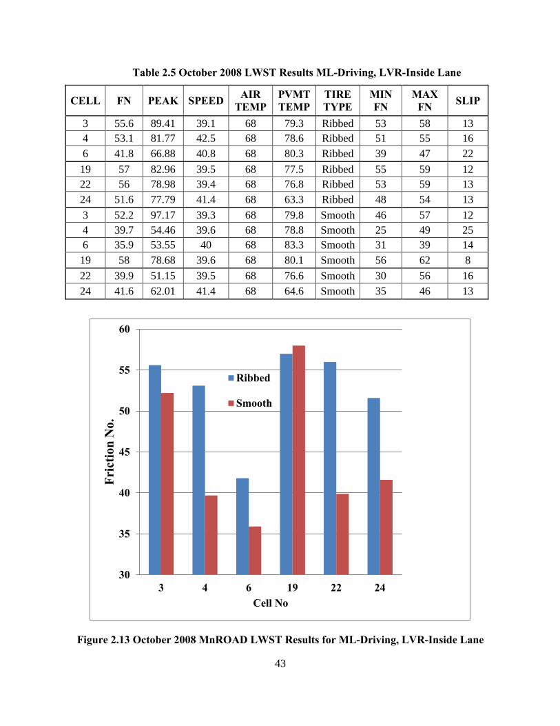
43
Table 2.5 October 2008 LWST Results ML-Driving, LVR-Inside Lane
CELL FN PEAK SPEED AIR TEMP
PVMT TEMP
TIRE TYPE
MIN FN
MAX FN SLIP
3 55.6 89.41 39.1 68 79.3 Ribbed 53 58 13 4 53.1 81.77 42.5 68 78.6 Ribbed 51 55 16 6 41.8 66.88 40.8 68 80.3 Ribbed 39 47 22 19 57 82.96 39.5 68 77.5 Ribbed 55 59 12 22 56 78.98 39.4 68 76.8 Ribbed 53 59 13 24 51.6 77.79 41.4 68 63.3 Ribbed 48 54 13 3 52.2 97.17 39.3 68 79.8 Smooth 46 57 12 4 39.7 54.46 39.6 68 78.8 Smooth 25 49 25 6 35.9 53.55 40 68 83.3 Smooth 31 39 14 19 58 78.68 39.6 68 80.1 Smooth 56 62 8 22 39.9 51.15 39.5 68 76.6 Smooth 30 56 16 24 41.6 62.01 41.4 68 64.6 Smooth 35 46 13
Figure 2.13 October 2008 MnROAD LWST Results for ML-Driving, LVR-Inside Lane
30
35
40
45
50
55
60
3 4 6 19 22 24
Fric
tion
No.
Cell No
Ribbed
Smooth
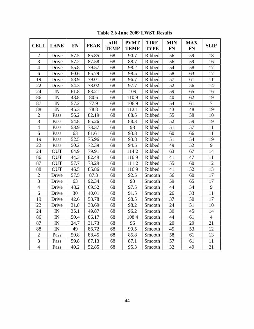
44
Table 2.6 June 2009 LWST Results
CELL LANE FN PEAK AIR TEMP
PVMT TEMP
TIRE TYPE
MIN FN
MAX FN SLIP
2 Drive 57.5 85.85 68 90.7 Ribbed 56 59 18 3 Drive 57.2 87.58 68 88.7 Ribbed 56 59 16 4 Drive 55.8 79.57 68 98.2 Ribbed 54 58 17 6 Drive 60.6 85.79 68 98.5 Ribbed 58 63 17 19 Drive 58.9 79.01 68 96.7 Ribbed 57 61 11 22 Drive 54.3 78.02 68 97.7 Ribbed 52 56 14 24 IN 61.8 83.21 68 109 Ribbed 59 65 16 86 IN 43.8 80.6 68 110.9 Ribbed 40 62 19 87 IN 57.2 77.9 68 106.9 Ribbed 54 61 7 88 IN 45.3 78.3 68 112.1 Ribbed 43 48 19 2 Pass 56.2 82.19 68 88.5 Ribbed 55 58 10 3 Pass 54.8 85.26 68 88.3 Ribbed 52 59 19 4 Pass 53.9 73.37 68 93 Ribbed 51 57 11 6 Pass 63 81.61 68 93.8 Ribbed 60 66 11 19 Pass 52.5 75.96 68 93.8 Ribbed 51 54 19 22 Pass 50.2 72.39 68 94.5 Ribbed 49 52 9 24 OUT 64.9 79.91 68 114.2 Ribbed 63 67 14 86 OUT 44.3 82.49 68 116.9 Ribbed 41 47 11 87 OUT 57.7 73.29 68 111.2 Ribbed 55 60 12 88 OUT 46.5 85.86 68 116.9 Ribbed 41 52 13 2 Drive 57.5 87.3 68 92.5 Smooth 56 60 17 3 Drive 63 92.34 68 93 Smooth 59 65 17 4 Drive 48.2 69.52 68 97.5 Smooth 44 54 9 6 Drive 30 40.01 68 91.5 Smooth 26 33 11 19 Drive 42.6 58.78 68 98.5 Smooth 37 50 17 22 Drive 31.8 38.69 68 98.2 Smooth 24 51 10 24 IN 35.1 49.87 68 96.2 Smooth 30 45 14 86 IN 50.4 86.17 68 108.4 Smooth 44 61 4 87 IN 24.7 31.73 68 96 Smooth 20 29 21 88 IN 49 86.72 68 99.5 Smooth 45 53 12 2 Pass 59.8 88.45 68 85.8 Smooth 58 61 13 3 Pass 59.8 87.13 68 87.1 Smooth 57 61 11 4 Pass 40.2 52.85 68 95.3 Smooth 32 49 21
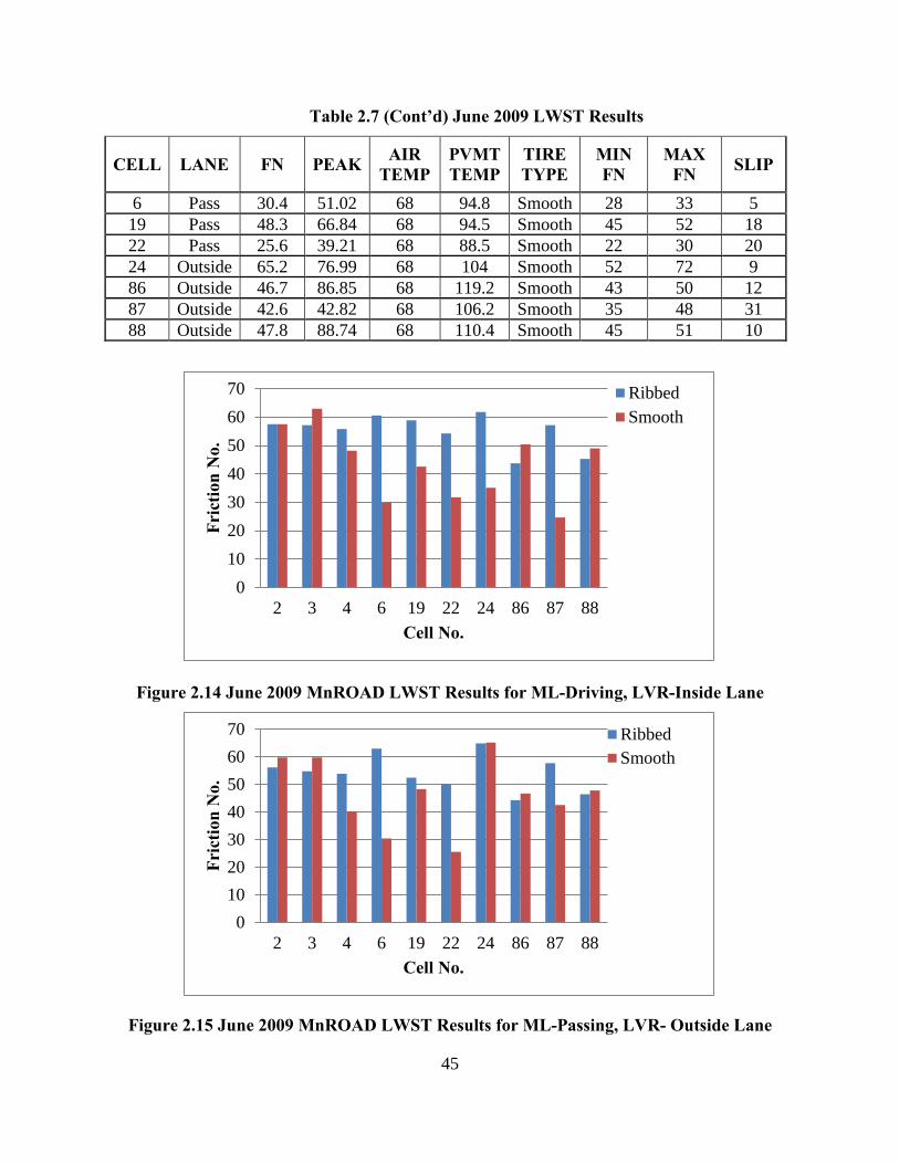
45
Table 2.7 (Cont’d) June 2009 LWST Results
CELL LANE FN PEAK AIR TEMP
PVMT TEMP
TIRE TYPE
MIN FN
MAX FN SLIP
6 Pass 30.4 51.02 68 94.8 Smooth 28 33 5 19 Pass 48.3 66.84 68 94.5 Smooth 45 52 18 22 Pass 25.6 39.21 68 88.5 Smooth 22 30 20 24 Outside 65.2 76.99 68 104 Smooth 52 72 9 86 Outside 46.7 86.85 68 119.2 Smooth 43 50 12 87 Outside 42.6 42.82 68 106.2 Smooth 35 48 31 88 Outside 47.8 88.74 68 110.4 Smooth 45 51 10
Figure 2.14 June 2009 MnROAD LWST Results for ML-Driving, LVR-Inside Lane
010203040506070
2 3 4 6 19 22 24 86 87 88
Fric
tion
No.
Cell No.
RibbedSmooth
Figure 2.15 June 2009 MnROAD LWST Results for ML-Passing, LVR- Outside Lane
010203040506070
2 3 4 6 19 22 24 86 87 88
Fric
tion
No.
Cell No.
RibbedSmooth
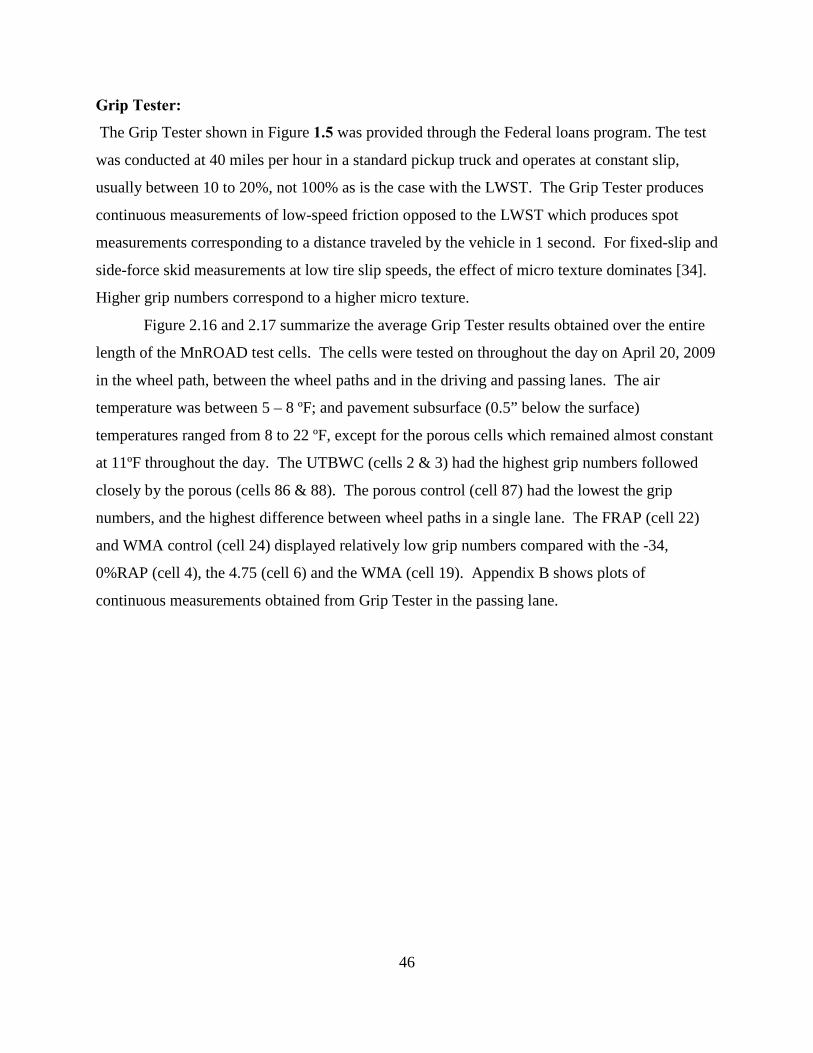
46
Grip Tester:
The Grip Tester shown in Figure 1.5 was provided through the Federal loans program. The test
was conducted at 40 miles per hour in a standard pickup truck and operates at constant slip,
usually between 10 to 20%, not 100% as is the case with the LWST. The Grip Tester produces
continuous measurements of low-speed friction opposed to the LWST which produces spot
measurements corresponding to a distance traveled by the vehicle in 1 second. For fixed-slip and
side-force skid measurements at low tire slip speeds, the effect of micro texture dominates [34].
Higher grip numbers correspond to a higher micro texture.
Figure 2.16 and 2.17 summarize the average Grip Tester results obtained over the entire
length of the MnROAD test cells. The cells were tested on throughout the day on April 20, 2009
in the wheel path, between the wheel paths and in the driving and passing lanes. The air
temperature was between 5 – 8 ºF; and pavement subsurface (0.5” below the surface)
temperatures ranged from 8 to 22 ºF, except for the porous cells which remained almost constant
at 11ºF throughout the day. The UTBWC (cells 2 & 3) had the highest grip numbers followed
closely by the porous (cells 86 & 88). The porous control (cell 87) had the lowest the grip
numbers, and the highest difference between wheel paths in a single lane. The FRAP (cell 22)
and WMA control (cell 24) displayed relatively low grip numbers compared with the -34,
0%RAP (cell 4), the 4.75 (cell 6) and the WMA (cell 19). Appendix B shows plots of
continuous measurements obtained from Grip Tester in the passing lane.
47
Figure 2.16 April 2009 MnROAD Grip Tester Results for ML-Driving, LVR-Inside Lane
Figure 2.17 April 2009 MnROAD Grip Tester Results for ML-Passing, LVR-Outside Lane
48
Dynamic Friction Tester:
The Dynamic Friction Tester (DFT) consists of three rubber sliders, positioned on a disk of
diameter 13.75 in, that are suspended above the pavement surface. When the tangential velocity
of the sliders reaches 90 km/hr water is applied to the surface and the sliders make contact with
the pavement. A computer takes friction measurements across a range of speeds as the sliders
slow to a stop. This test was just recently acquired by MnDOT using project funds, and
consequently measurements will be included in a later report.
RIDE
Ames Light Weight Profiler Measurements: Ride was measured in both the left and right wheel paths of the driving and passing lanes using
an Ames lightweight inertial surface analyzer (LISA) as shown in Figures 2.18 and 2.19. The
testing took place on November 19, 2008 following construction. The results were separated into
cells by cropping the start and end stations of each of the cells. Figure 2.18 and 2.19 show a comparative plot of the average ride for the entire length of
the study cells in terms of IRI (in/mi) for the driving and passing lanes respectively. In the
driving lane, the UTBWC (cells 2 & 3) had the lowest IRI, followed by the FRAP (cell 22) and
in the passing lane the WM (cell 19) and the FRAP (cell 22) had the lowest IRI. In the driving
lane, the 4.75 (cell 6) appears to have the highest IRI, and in the passing lane, the -34, 0%RAP
had the highest IRI followed by the 4.75 (cell 6) and the UTBWC (cells 2 & 3). The -34,
0%RAP (cell 4) and the WMA (cell 19) appear to have large differences between the LWP and
RWP in the driving and passing lanes and large differences between the driving and passing
lanes. Figure 2.20 shows the measured profile of cell 3, in the left wheel path of the driving lane;
plots of the remaining cells: 4, 6, 19 and 22 can be found in Appendix 2.B. At this stage the
lightweight profiler was equipped with a line laser and a triple spot laser which helped with
evaluation of texture influence on IRI.
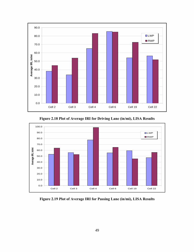
49
Figure 2.18 Plot of Average IRI for Driving Lane (in/mi), LISA Results
0.0
10.0
20.0
30.0
40.0
50.0
60.0
70.0
80.0
90.0
Cell 2 Cell 3 Cell 4 Cell 6 Cell 19 Cell 22
Aver
age
IRI,
in/m
iLWP
RWP
Figure 2.19 Plot of Average IRI for Passing Lane (in/mi), LISA Results
0.0
10.0
20.0
30.0
40.0
50.0
60.0
70.0
80.0
90.0
100.0
Cell 2 Cell 3 Cell 4 Cell 6 Cell 19 Cell 22
Aver
age I
RI, in
/mi
LWP
RWP
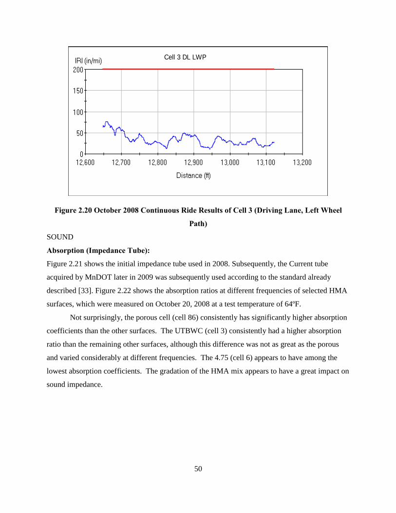
50
Figure 2.20 October 2008 Continuous Ride Results of Cell 3 (Driving Lane, Left Wheel
Path)
Cell 3 DL LWP
SOUND
Absorption (Impedance Tube):
Figure 2.21 shows the initial impedance tube used in 2008. Subsequently, the Current tube
acquired by MnDOT later in 2009 was subsequently used according to the standard already
described [33]. Figure 2.22 shows the absorption ratios at different frequencies of selected HMA
surfaces, which were measured on October 20, 2008 at a test temperature of 64ºF.
Not surprisingly, the porous cell (cell 86) consistently has significantly higher absorption
coefficients than the other surfaces. The UTBWC (cell 3) consistently had a higher absorption
ratio than the remaining other surfaces, although this difference was not as great as the porous
and varied considerably at different frequencies. The 4.75 (cell 6) appears to have among the
lowest absorption coefficients. The gradation of the HMA mix appears to have a great impact on
sound impedance.
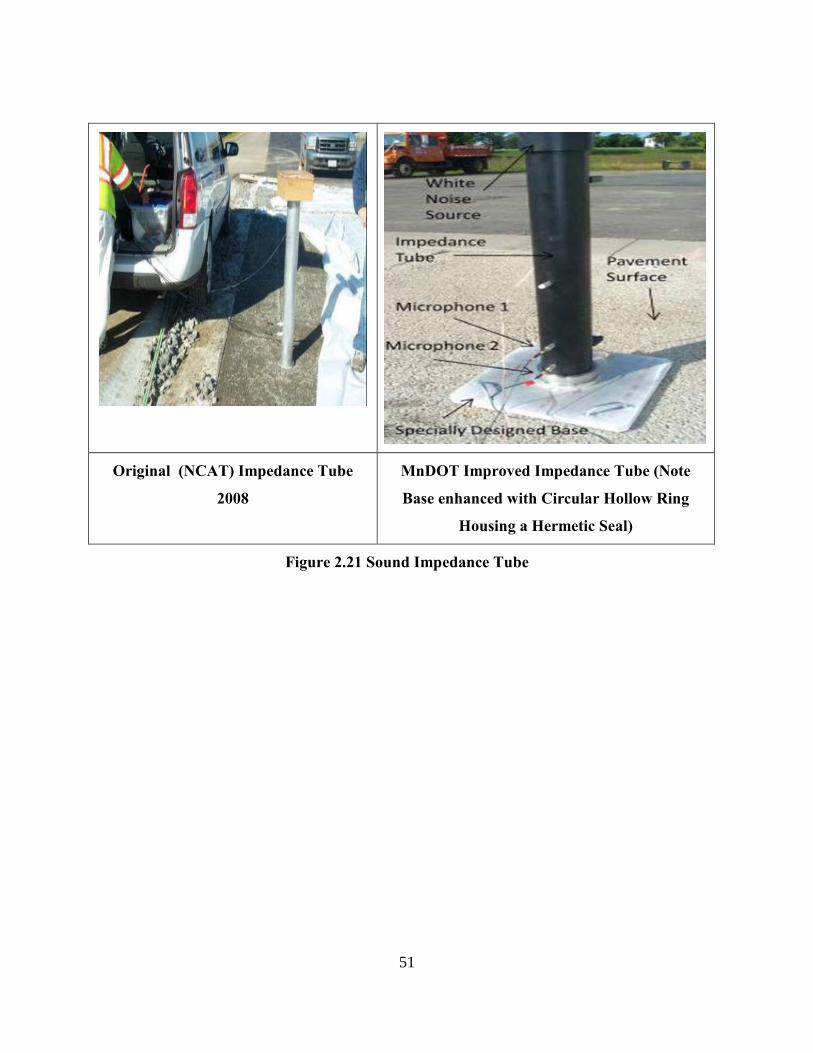
51
Figure 2.21 Sound Impedance Tube
Original (NCAT) Impedance Tube
2008
MnDOT Improved Impedance Tube (Note
Base enhanced with Circular Hollow Ring
Housing a Hermetic Seal)
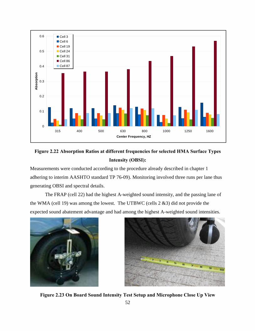
52
Figure 2.22 Absorption Ratios at different frequencies for selected HMA Surface Types
0
0.1
0.2
0.3
0.4
0.5
0.6
315 400 500 630 800 1000 1250 1600
Center Frequency, HZ
Abs
orpt
ion
Cell 3Cell 6Cell 19Cell 24Cell 31Cell 86Cell 87
Intensity (OBSI):
Measurements were conducted according to the procedure already described in chapter 1
adhering to interim AASHTO standard TP 76-09). Monitoring involved three runs per lane thus
generating OBSI and spectral details.
The FRAP (cell 22) had the highest A-weighted sound intensity, and the passing lane of
the WMA (cell 19) was among the lowest. The UTBWC (cells 2 &3) did not provide the
expected sound abatement advantage and had among the highest A-weighted sound intensities.
Figure 2.23 On Board Sound Intensity Test Setup and Microphone Close Up View
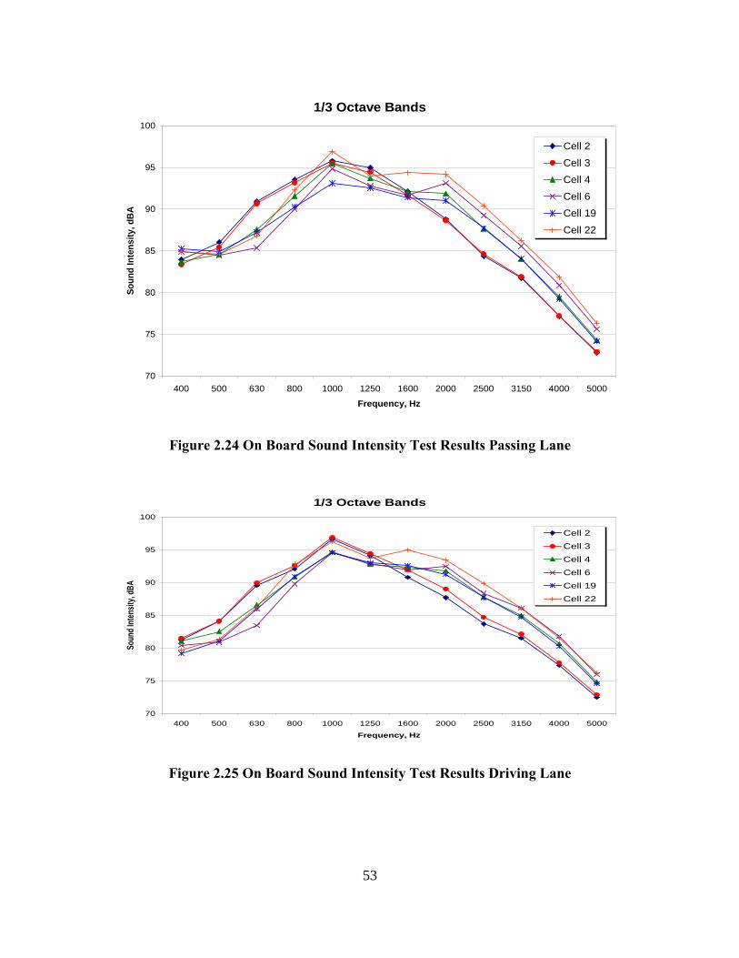
53
Figure 2.24 On Board Sound Intensity Test Results Passing Lane
1/3 Octave Bands
70
75
80
85
90
95
100
400 500 630 800 1000 1250 1600 2000 2500 3150 4000 5000
Frequency, Hz
Soun
d In
tens
ity, d
BA
Cell 2
Cell 3
Cell 4
Cell 6
Cell 19
Cell 22
Figure 2.25 On Board Sound Intensity Test Results Driving Lane
1/3 Octave Bands
70
75
80
85
90
95
100
400 500 630 800 1000 1250 1600 2000 2500 3150 4000 5000
Frequency, Hz
Soun
d Int
ensit
y, dB
A
Cell 2
Cell 3
Cell 4
Cell 6
Cell 19
Cell 22
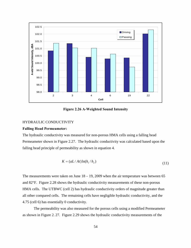
54
Figure 2.26 A-Weighted Sound Intensity
98.0
98.5
99.0
99.5
100.0
100.5
101.0
101.5
102.0
102.5
2 3 4 6 19 22
Cell
A-wt
d So
und
Inte
nsity
, dBA
Driving
Passing
HYDRAULIC CONDUCTIVITY
Falling Head Permeameter:
The hydraulic conductivity was measured for non-porous HMA cells using a falling head
Permeameter shown in Figure 2.27. The hydraulic conductivity was calculated based upon the
falling head principle of permeability as shown in equation 4.
(11) )/ln()/( 21 hhAtaLK =
The measurements were taken on June 18 – 19, 2009 when the air temperature was between 65
and 82°F. Figure 2.28 shows the hydraulic conductivity measurements of these non-porous
HMA cells. The UTBWC (cell 2) has hydraulic conductivity orders of magnitude greater than
all other compared cells. The remaining cells have negligible hydraulic conductivity, and the
4.75 (cell 6) has essentially 0 conductivity.
The permeability was also measured for the porous cells using a modified Permeameter
as shown in Figure 2. 27. Figure 2.29 shows the hydraulic conductivity measurements of the
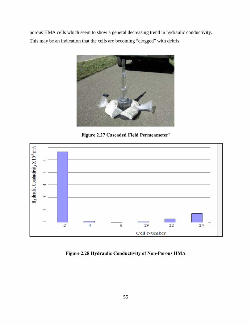
55
porous HMA cells which seem to show a general decreasing trend in hydraulic conductivity.
This may be an indication that the cells are becoming “clogged” with debris.
Figure 2.27 Cascaded Field Permeameter’
Figure 2.28 Hydraulic Conductivity of Non-Porous HMA
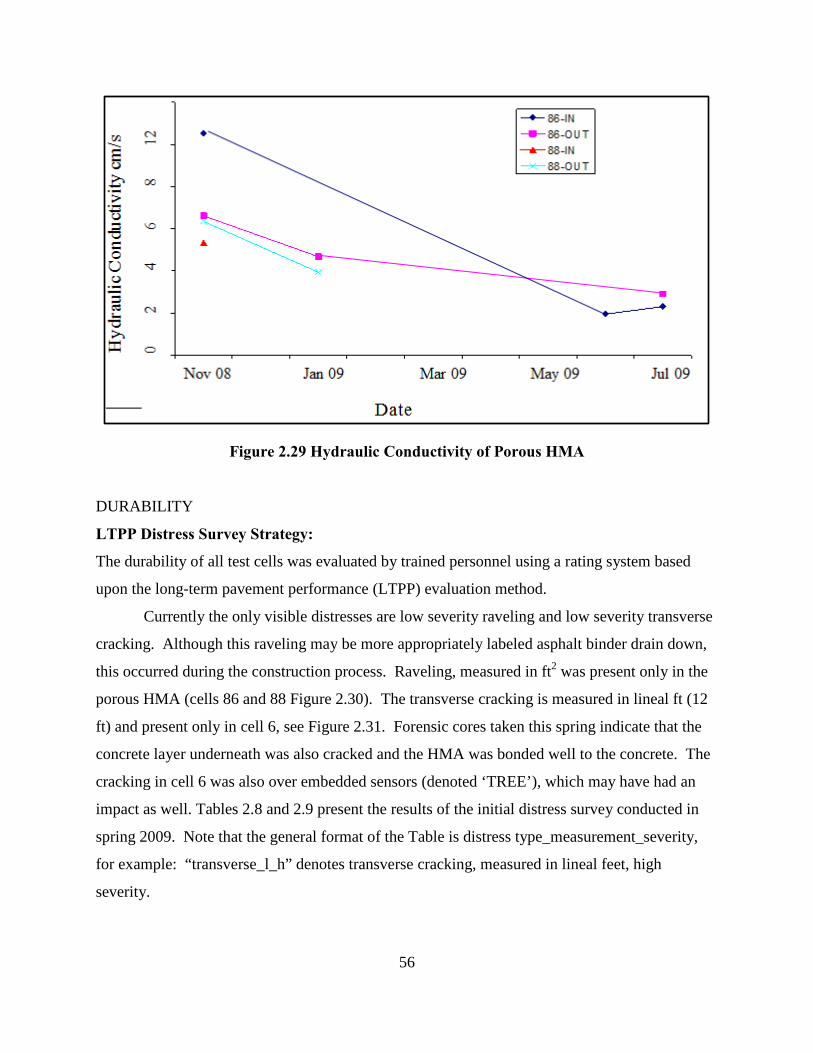
56
Figure 2.29 Hydraulic Conductivity of Porous HMA
DURABILITY LTPP Distress Survey Strategy:
The durability of all test cells was evaluated by trained personnel using a rating system based
upon the long-term pavement performance (LTPP) evaluation method.
Currently the only visible distresses are low severity raveling and low severity transverse
cracking. Although this raveling may be more appropriately labeled asphalt binder drain down,
this occurred during the construction process. Raveling, measured in ft2 was present only in the
porous HMA (cells 86 and 88 Figure 2.30). The transverse cracking is measured in lineal ft (12
ft) and present only in cell 6, see Figure 2.31. Forensic cores taken this spring indicate that the
concrete layer underneath was also cracked and the HMA was bonded well to the concrete. The
cracking in cell 6 was also over embedded sensors (denoted ‘TREE’), which may have had an
impact as well. Tables 2.8 and 2.9 present the results of the initial distress survey conducted in
spring 2009. Note that the general format of the Table is distress type_measurement_severity,
for example: “transverse_l_h” denotes transverse cracking, measured in lineal feet, high
severity.
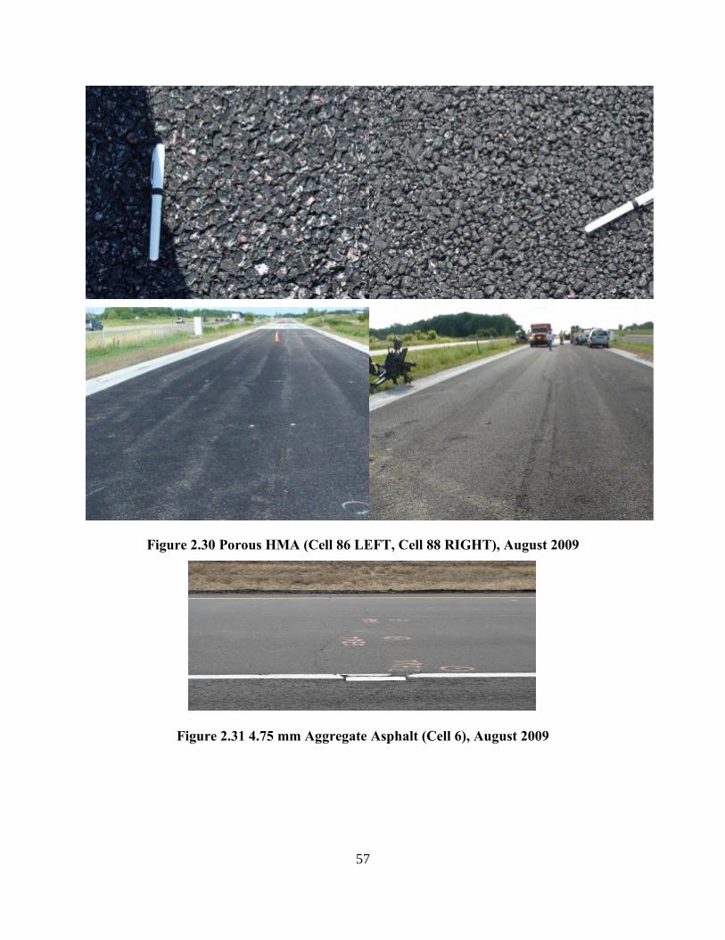
57
Figure 2.30 Porous HMA (Cell 86 LEFT, Cell 88 RIGHT), August 2009
Figure 2.31 4.75 mm Aggregate Asphalt (Cell 6), August 2009
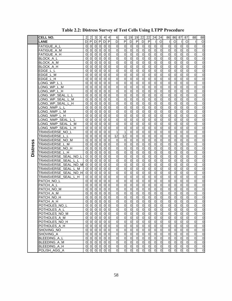
58
Table 2.2: Distress Survey of Test Cells Using LTPP Procedure
CELL NO. 2 2 3 3 4 4 6 6 19 19 22 22 24 24 86 86 87 87 88 88LANE D P D P D P D P D P D P I O I O I O I OFATIGUE_A_L 0 0 0 0 0 0 0 0 0 0 0 0 0 0 0 0 0 0 0 0FATIGUE_A_M 0 0 0 0 0 0 0 0 0 0 0 0 0 0 0 0 0 0 0 0FATIGUE_A_H 0 0 0 0 0 0 0 0 0 0 0 0 0 0 0 0 0 0 0 0BLOCK_A_L 0 0 0 0 0 0 0 0 0 0 0 0 0 0 0 0 0 0 0 0BLOCK_A_M 0 0 0 0 0 0 0 0 0 0 0 0 0 0 0 0 0 0 0 0BLOCK_A_H 0 0 0 0 0 0 0 0 0 0 0 0 0 0 0 0 0 0 0 0EDGE_L_L 0 0 0 0 0 0 0 0 0 0 0 0 0 0 0 0 0 0 0 0EDGE_L_M 0 0 0 0 0 0 0 0 0 0 0 0 0 0 0 0 0 0 0 0EDGE_L_H 0 0 0 0 0 0 0 0 0 0 0 0 0 0 0 0 0 0 0 0LONG_WP_L_L 0 0 0 0 0 0 0 0 0 0 0 0 0 0 0 0 0 0 0 0LONG_WP_L_M 0 0 0 0 0 0 0 0 0 0 0 0 0 0 0 0 0 0 0 0LONG_WP_L_H 0 0 0 0 0 0 0 0 0 0 0 0 0 0 0 0 0 0 0 0LONG_WP_SEAL_L_L 0 0 0 0 0 0 0 0 0 0 0 0 0 0 0 0 0 0 0 0LONG_WP_SEAL_L_M 0 0 0 0 0 0 0 0 0 0 0 0 0 0 0 0 0 0 0 0LONG_WP_SEAL_L_H 0 0 0 0 0 0 0 0 0 0 0 0 0 0 0 0 0 0 0 0LONG_NWP_L_L 0 0 0 0 0 0 0 0 0 0 0 0 0 0 0 0 0 0 0 0LONG_NWP_L_M 0 0 0 0 0 0 0 0 0 0 0 0 0 0 0 0 0 0 0 0LONG_NWP_L_H 0 0 0 0 0 0 0 0 0 0 0 0 0 0 0 0 0 0 0 0LONG_NWP_SEAL_L_L 0 0 0 0 0 0 0 0 0 0 0 0 0 0 0 0 0 0 0 0LONG_NWP_SEAL_L_M 0 0 0 0 0 0 0 0 0 0 0 0 0 0 0 0 0 0 0 0LONG_NWP_SEAL_L_H 0 0 0 0 0 0 0 0 0 0 0 0 0 0 0 0 0 0 0 0TRANSVERSE_NO_L 0 0 0 0 0 0 1 1 0 0 0 0 0 0 0 0 0 0 0 0TRANSVERSE_L_L 0 0 0 0 0 0 12 12 0 0 0 0 0 0 0 0 0 0 0 0TRANSVERSE_NO_M 0 0 0 0 0 0 0 0 0 0 0 0 0 0 0 0 0 0 0 0TRANSVERSE_L_M 0 0 0 0 0 0 0 0 0 0 0 0 0 0 0 0 0 0 0 0TRANSVERSE_NO_H 0 0 0 0 0 0 0 0 0 0 0 0 0 0 0 0 0 0 0 0TRANSVERSE_L_H 0 0 0 0 0 0 0 0 0 0 0 0 0 0 0 0 0 0 0 0TRANSVERSE_SEAL_NO_L 0 0 0 0 0 0 0 0 0 0 0 0 0 0 0 0 0 0 0 0TRANSVERSE_SEAL_L_L 0 0 0 0 0 0 0 0 0 0 0 0 0 0 0 0 0 0 0 0TRANSVERSE_SEAL_NO_M 0 0 0 0 0 0 0 0 0 0 0 0 0 0 0 0 0 0 0 0TRANSVERSE_SEAL_L_M 0 0 0 0 0 0 0 0 0 0 0 0 0 0 0 0 0 0 0 0TRANSVERSE_SEAL_NO_H 0 0 0 0 0 0 0 0 0 0 0 0 0 0 0 0 0 0 0 0TRANSVERSE_SEAL_L_H 0 0 0 0 0 0 0 0 0 0 0 0 0 0 0 0 0 0 0 0PATCH_NO_L 0 0 0 0 0 0 0 0 0 0 0 0 0 0 0 0 0 0 0 0PATCH_A_L 0 0 0 0 0 0 0 0 0 0 0 0 0 0 0 0 0 0 0 0PATCH_NO_M 0 0 0 0 0 0 0 0 0 0 0 0 0 0 0 0 0 0 0 0PATCH_A_M 0 0 0 0 0 0 0 0 0 0 0 0 0 0 0 0 0 0 0 0PATCH_NO_H 0 0 0 0 0 0 0 0 0 0 0 0 0 0 0 0 0 0 0 0PATCH_A_H 0 0 0 0 0 0 0 0 0 0 0 0 0 0 0 0 0 0 0 0POTHOLES_NO_L 0 0 0 0 0 0 0 0 0 0 0 0 0 0 0 0 0 0 0 0POTHOLES_A_L 0 0 0 0 0 0 0 0 0 0 0 0 0 0 0 0 0 0 0 0POTHOLES_NO_M 0 0 0 0 0 0 0 0 0 0 0 0 0 0 0 0 0 0 0 0POTHOLES_A_M 0 0 0 0 0 0 0 0 0 0 0 0 0 0 0 0 0 0 0 0POTHOLES_NO_H 0 0 0 0 0 0 0 0 0 0 0 0 0 0 0 0 0 0 0 0POTHOLES_A_H 0 0 0 0 0 0 0 0 0 0 0 0 0 0 0 0 0 0 0 0SHOVING_NO 0 0 0 0 0 0 0 0 0 0 0 0 0 0 0 0 0 0 0 0SHOVING_A 0 0 0 0 0 0 0 0 0 0 0 0 0 0 0 0 0 0 0 0BLEEDING_A_L 0 0 0 0 0 0 0 0 0 0 0 0 0 0 0 0 0 0 0 0BLEEDING_A_M 0 0 0 0 0 0 0 0 0 0 0 0 0 0 0 0 0 0 0 0BLEEDING_A_H 0 0 0 0 0 0 0 0 0 0 0 0 0 0 0 0 0 0 0 0POLISH_AGG_A 0 0 0 0 0 0 0 0 0 0 0 0 0 0 0 0 0 0 0 0
Dis
tres
s
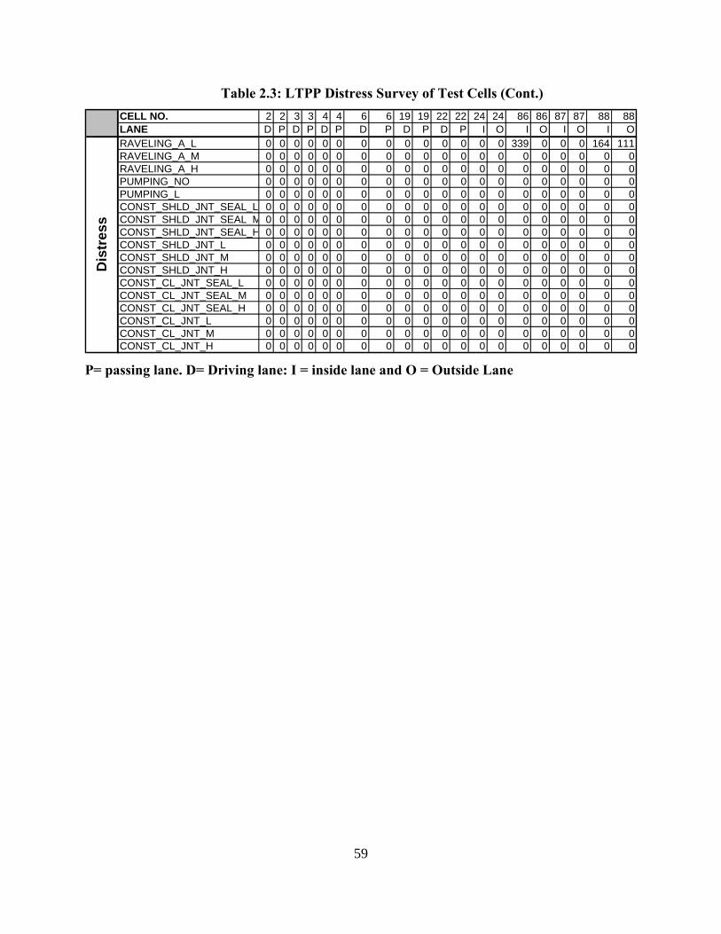
59
Table 2.3: LTPP Distress Survey of Test Cells (Cont.)
CELL NO. 2 2 3 3 4 4 6 6 19 19 22 22 24 24 86 86 87 87 88 88LANE D P D P D P D P D P D P I O I O I O I ORAVELING_A_L 0 0 0 0 0 0 0 0 0 0 0 0 0 0 339 0 0 0 164 111RAVELING_A_M 0 0 0 0 0 0 0 0 0 0 0 0 0 0 0 0 0 0 0 0RAVELING_A_H 0 0 0 0 0 0 0 0 0 0 0 0 0 0 0 0 0 0 0 0PUMPING_NO 0 0 0 0 0 0 0 0 0 0 0 0 0 0 0 0 0 0 0 0PUMPING_L 0 0 0 0 0 0 0 0 0 0 0 0 0 0 0 0 0 0 0 0CONST_SHLD_JNT_SEAL_L 0 0 0 0 0 0 0 0 0 0 0 0 0 0 0 0 0 0 0 0CONST_SHLD_JNT_SEAL_M 0 0 0 0 0 0 0 0 0 0 0 0 0 0 0 0 0 0 0 0CONST_SHLD_JNT_SEAL_H 0 0 0 0 0 0 0 0 0 0 0 0 0 0 0 0 0 0 0 0CONST_SHLD_JNT_L 0 0 0 0 0 0 0 0 0 0 0 0 0 0 0 0 0 0 0 0CONST_SHLD_JNT_M 0 0 0 0 0 0 0 0 0 0 0 0 0 0 0 0 0 0 0 0CONST_SHLD_JNT_H 0 0 0 0 0 0 0 0 0 0 0 0 0 0 0 0 0 0 0 0CONST_CL_JNT_SEAL_L 0 0 0 0 0 0 0 0 0 0 0 0 0 0 0 0 0 0 0 0CONST_CL_JNT_SEAL_M 0 0 0 0 0 0 0 0 0 0 0 0 0 0 0 0 0 0 0 0CONST_CL_JNT_SEAL_H 0 0 0 0 0 0 0 0 0 0 0 0 0 0 0 0 0 0 0 0CONST_CL_JNT_L 0 0 0 0 0 0 0 0 0 0 0 0 0 0 0 0 0 0 0 0CONST_CL_JNT_M 0 0 0 0 0 0 0 0 0 0 0 0 0 0 0 0 0 0 0 0CONST_CL_JNT_H 0 0 0 0 0 0 0 0 0 0 0 0 0 0 0 0 0 0 0 0
Dis
tres
s
P= passing lane. D= Driving lane: I = inside lane and O = Outside Lane
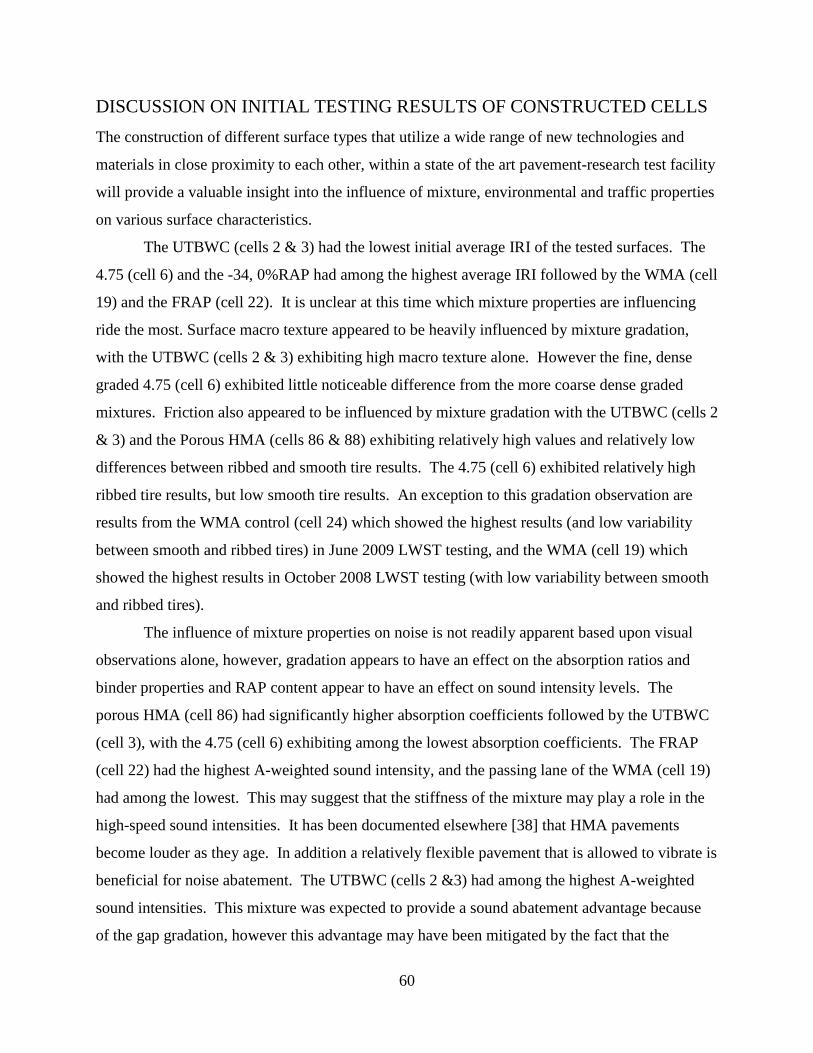
60
DISCUSSION ON INITIAL TESTING RESULTS OF CONSTRUCTED CELLS The construction of different surface types that utilize a wide range of new technologies and
materials in close proximity to each other, within a state of the art pavement-research test facility
will provide a valuable insight into the influence of mixture, environmental and traffic properties
on various surface characteristics.
The UTBWC (cells 2 & 3) had the lowest initial average IRI of the tested surfaces. The
4.75 (cell 6) and the -34, 0%RAP had among the highest average IRI followed by the WMA (cell
19) and the FRAP (cell 22). It is unclear at this time which mixture properties are influencing
ride the most. Surface macro texture appeared to be heavily influenced by mixture gradation,
with the UTBWC (cells 2 & 3) exhibiting high macro texture alone. However the fine, dense
graded 4.75 (cell 6) exhibited little noticeable difference from the more coarse dense graded
mixtures. Friction also appeared to be influenced by mixture gradation with the UTBWC (cells 2
& 3) and the Porous HMA (cells 86 & 88) exhibiting relatively high values and relatively low
differences between ribbed and smooth tire results. The 4.75 (cell 6) exhibited relatively high
ribbed tire results, but low smooth tire results. An exception to this gradation observation are
results from the WMA control (cell 24) which showed the highest results (and low variability
between smooth and ribbed tires) in June 2009 LWST testing, and the WMA (cell 19) which
showed the highest results in October 2008 LWST testing (with low variability between smooth
and ribbed tires).
The influence of mixture properties on noise is not readily apparent based upon visual
observations alone, however, gradation appears to have an effect on the absorption ratios and
binder properties and RAP content appear to have an effect on sound intensity levels. The
porous HMA (cell 86) had significantly higher absorption coefficients followed by the UTBWC
(cell 3), with the 4.75 (cell 6) exhibiting among the lowest absorption coefficients. The FRAP
(cell 22) had the highest A-weighted sound intensity, and the passing lane of the WMA (cell 19)
had among the lowest. This may suggest that the stiffness of the mixture may play a role in the
high-speed sound intensities. It has been documented elsewhere [38] that HMA pavements
become louder as they age. In addition a relatively flexible pavement that is allowed to vibrate is
beneficial for noise abatement. The UTBWC (cells 2 &3) had among the highest A-weighted
sound intensities. This mixture was expected to provide a sound abatement advantage because
of the gap gradation, however this advantage may have been mitigated by the fact that the

61
UTBWC is a relatively stiff mixture and thus not able to vibrate as much as other mixtures.
Durability only appears to be an issue for the porous HMA (cells 86 & 88) as these
sections are already experiencing raveling after their first winter. The 4.75 (cell 6) is the only
cell experiencing cracking, but this crack is near embedded instrumentation and over a crack in
the underlying PCC pavement, which may have influenced the crack development. The UTBWC
(cells 2 & 3) had the lowest average IRI of the tested surfaces. The 4.75 (cell 6) and the -34,
0%RAP had among the highest average IRI followed by the WMA (cell 19) and the FRAP (cell
22). It is unclear at this time which mixture properties are influencing ride the most.

62
CHAPTER 3
SEASONAL MEASUREMENTS OF SURFACE: 4TH YEAR
CHARACTERISTICS (2012)
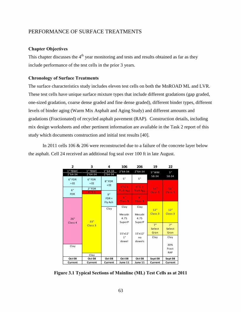
63
PERFORMANCE OF SURFACE TREATMENTS
Chapter Objectives
This chapter discusses the 4th year monitoring and tests and results obtained as far as they
include performance of the test cells in the prior 3 years.
Chronology of Surface Treatments
The surface characteristics study includes eleven test cells on both the MnROAD ML and LVR.
These test cells have unique surface mixture types that include different gradations (gap graded,
one-sized gradation, coarse dense graded and fine dense graded), different binder types, different
levels of binder aging (Warm Mix Asphalt and Aging Study) and different amounts and
gradations (Fractionated) of recycled asphalt pavement (RAP). Construction details, including
mix design worksheets and other pertinent information are available in the Task 2 report of this
study which documents construction and initial test results [40].
In 2011 cells 106 & 206 were reconstructed due to a failure of the concrete layer below
the asphalt. Cell 24 received an additional fog seal over 100 ft in late August.
Figure 3.1 Typical Sections of Mainline (ML) Test Cells as at 2011
2 3 4 106 206 19 221" TBWC 1" TBWC 1" 64-34
Oct 08 Oct 08 Oct 08 Oct 08 Oct 08 Sept 08 Sept 08Current Current Current June 11 June 11 Current Current
5" WM58-34
12"Class 5
12"Class 3
7"SelectGran
Clay
5"58-34
12"Class 5
12"Class 3
7"SelectGran
Clay
30%FractRAP
2"64-34 2"64-34
5" 5"
6" Cl 1Stab Agg
6" Cl 1Stab Agg
6"Class 5
6"Class 5
Clay
Mesabi4.75
SuperP
15'x12'1"
dowel
Clay
Mesabi4.75
SuperP
15'x12'no
dowels
2"64-34
8" FDR+ EE
9" FDR +
Fly Ash
Clay
2"64-34
6" FDR+ EE
6"FDR
26"Class 4
Clay
2"64-34
6" FDR+ EE
2" FDR2"Cl 5
33"Class 3
Clay
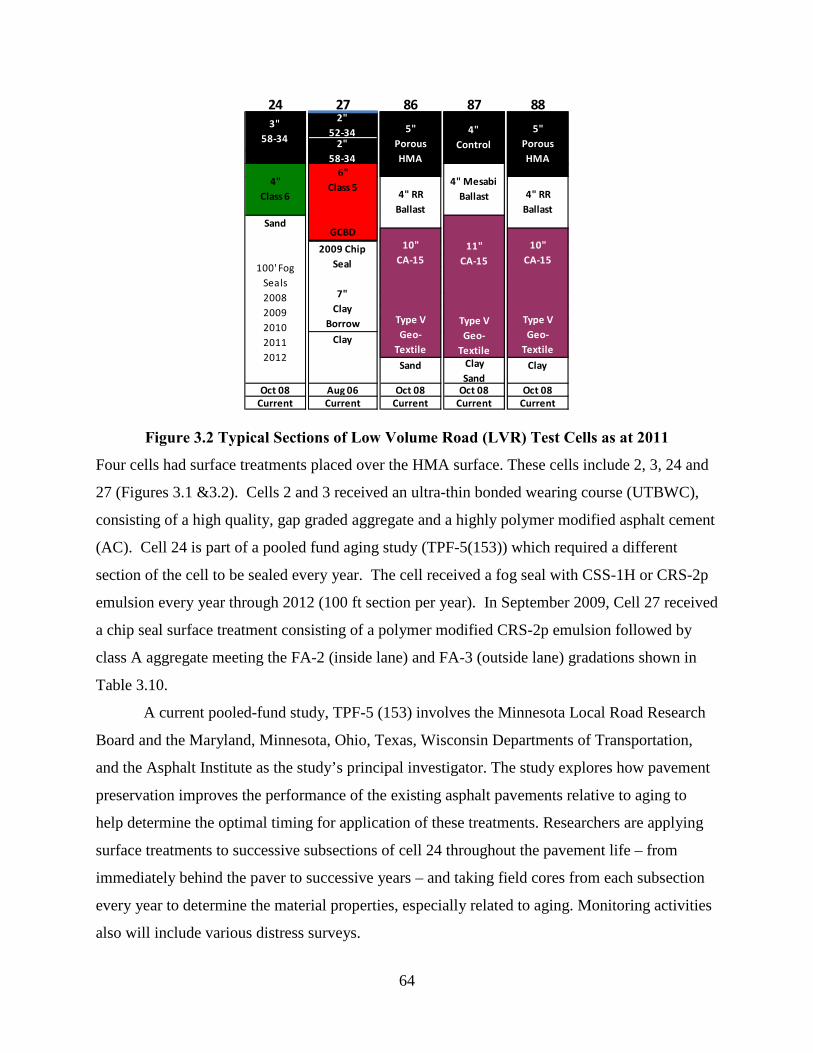
64
Figure 3.2 Typical Sections of Low Volume Road (LVR) Test Cells as at 2011
24 27 86 87 88
Oct 08 Aug 06 Oct 08 Oct 08 Oct 08Current Current Current Current Current
Clay
Sand ClaySand
Clay
11"CA-15
Type VGeo-
Textile
10"CA-15
Type VGeo-
Textile
10"CA-15
Type VGeo-
Textile
2009 Chip Seal
7"Clay
Borrow
2"58-34
4" MesabiBallast
6"Class 5
GCBD
2"52-34 5"
PorousHMA
4"Control
5"PorousHMA
4" RRBallast
4" RRBallast
Sand
100' Fog Seals 20082009201020112012
4"Class 6
3"58-34
Four cells had surface treatments placed over the HMA surface. These cells include 2, 3, 24 and
27 (Figures 3.1 &3.2). Cells 2 and 3 received an ultra-thin bonded wearing course (UTBWC),
consisting of a high quality, gap graded aggregate and a highly polymer modified asphalt cement
(AC). Cell 24 is part of a pooled fund aging study (TPF-5(153)) which required a different
section of the cell to be sealed every year. The cell received a fog seal with CSS-1H or CRS-2p
emulsion every year through 2012 (100 ft section per year). In September 2009, Cell 27 received
a chip seal surface treatment consisting of a polymer modified CRS-2p emulsion followed by
class A aggregate meeting the FA-2 (inside lane) and FA-3 (outside lane) gradations shown in
Table 3.10.
A current pooled-fund study, TPF-5 (153) involves the Minnesota Local Road Research
Board and the Maryland, Minnesota, Ohio, Texas, Wisconsin Departments of Transportation,
and the Asphalt Institute as the study’s principal investigator. The study explores how pavement
preservation improves the performance of the existing asphalt pavements relative to aging to
help determine the optimal timing for application of these treatments. Researchers are applying
surface treatments to successive subsections of cell 24 throughout the pavement life – from
immediately behind the paver to successive years – and taking field cores from each subsection
every year to determine the material properties, especially related to aging. Monitoring activities
also will include various distress surveys.
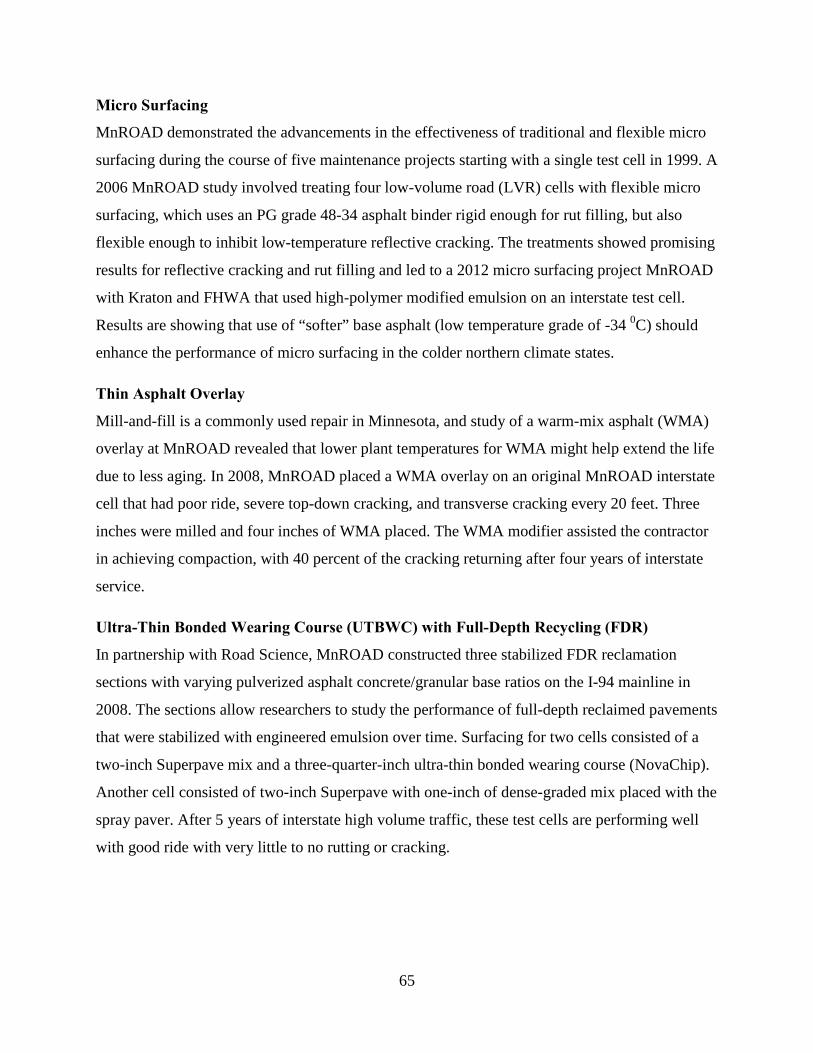
65
Micro Surfacing
MnROAD demonstrated the advancements in the effectiveness of traditional and flexible micro
surfacing during the course of five maintenance projects starting with a single test cell in 1999. A
2006 MnROAD study involved treating four low-volume road (LVR) cells with flexible micro
surfacing, which uses an PG grade 48-34 asphalt binder rigid enough for rut filling, but also
flexible enough to inhibit low-temperature reflective cracking. The treatments showed promising
results for reflective cracking and rut filling and led to a 2012 micro surfacing project MnROAD
with Kraton and FHWA that used high-polymer modified emulsion on an interstate test cell.
Results are showing that use of “softer” base asphalt (low temperature grade of -34 0C) should
enhance the performance of micro surfacing in the colder northern climate states.
Thin Asphalt Overlay
Mill-and-fill is a commonly used repair in Minnesota, and study of a warm-mix asphalt (WMA)
overlay at MnROAD revealed that lower plant temperatures for WMA might help extend the life
due to less aging. In 2008, MnROAD placed a WMA overlay on an original MnROAD interstate
cell that had poor ride, severe top-down cracking, and transverse cracking every 20 feet. Three
inches were milled and four inches of WMA placed. The WMA modifier assisted the contractor
in achieving compaction, with 40 percent of the cracking returning after four years of interstate
service.
Ultra-Thin Bonded Wearing Course (UTBWC) with Full-Depth Recycling (FDR)
In partnership with Road Science, MnROAD constructed three stabilized FDR reclamation
sections with varying pulverized asphalt concrete/granular base ratios on the I-94 mainline in
2008. The sections allow researchers to study the performance of full-depth reclaimed pavements
that were stabilized with engineered emulsion over time. Surfacing for two cells consisted of a
two-inch Superpave mix and a three-quarter-inch ultra-thin bonded wearing course (NovaChip).
Another cell consisted of two-inch Superpave with one-inch of dense-graded mix placed with the
spray paver. After 5 years of interstate high volume traffic, these test cells are performing well
with good ride with very little to no rutting or cracking.
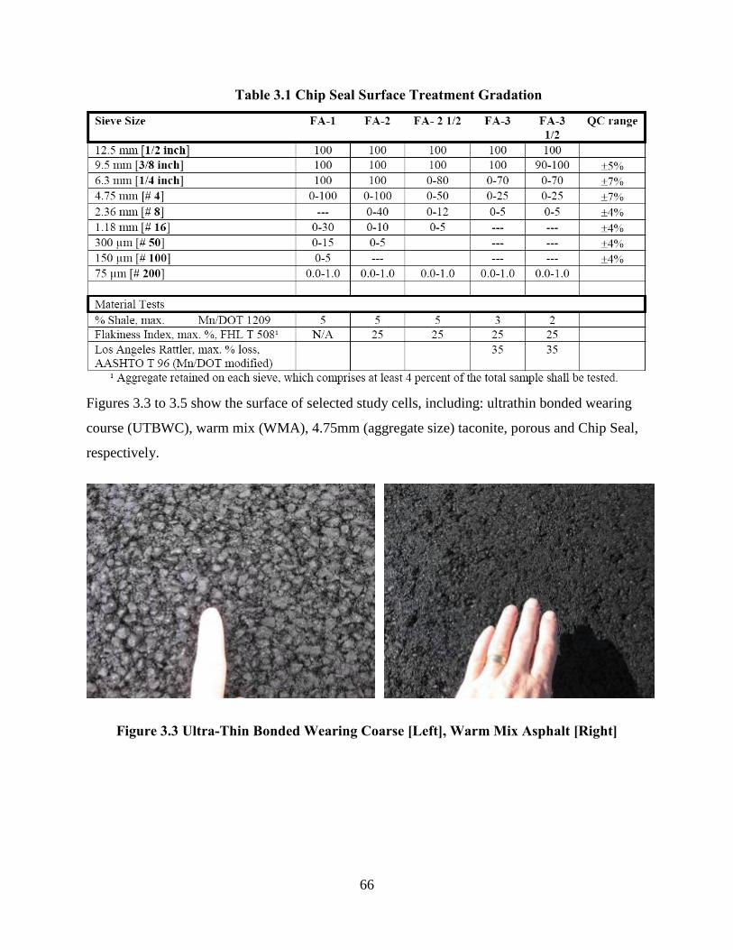
66
Table 3.1 Chip Seal Surface Treatment Gradation
Figures 3.3 to 3.5 show the surface of selected study cells, including: ultrathin bonded wearing
course (UTBWC), warm mix (WMA), 4.75mm (aggregate size) taconite, porous and Chip Seal,
respectively.
Figure 3.3 Ultra-Thin Bonded Wearing Coarse [Left], Warm Mix Asphalt [Right]
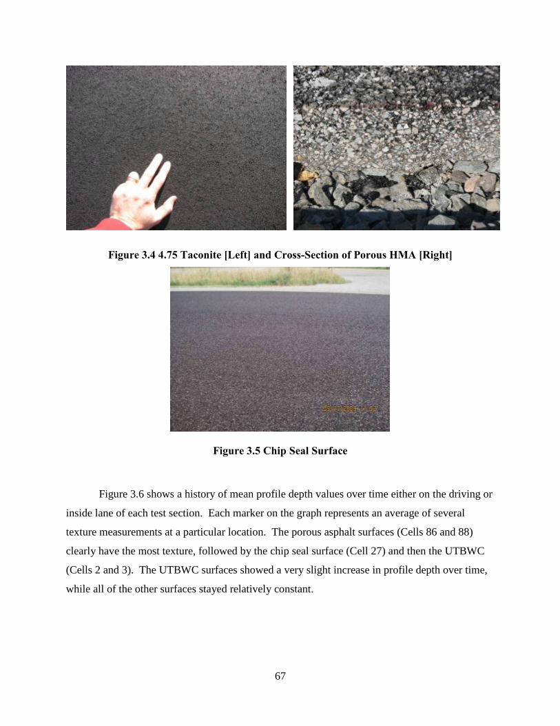
67
Figure 3.4 4.75 Taconite [Left] and Cross-Section of Porous HMA [Right]
Figure 3.5 Chip Seal Surface
Figure 3.6 shows a history of mean profile depth values over time either on the driving or
inside lane of each test section. Each marker on the graph represents an average of several
texture measurements at a particular location. The porous asphalt surfaces (Cells 86 and 88)
clearly have the most texture, followed by the chip seal surface (Cell 27) and then the UTBWC
(Cells 2 and 3). The UTBWC surfaces showed a very slight increase in profile depth over time,
while all of the other surfaces stayed relatively constant.
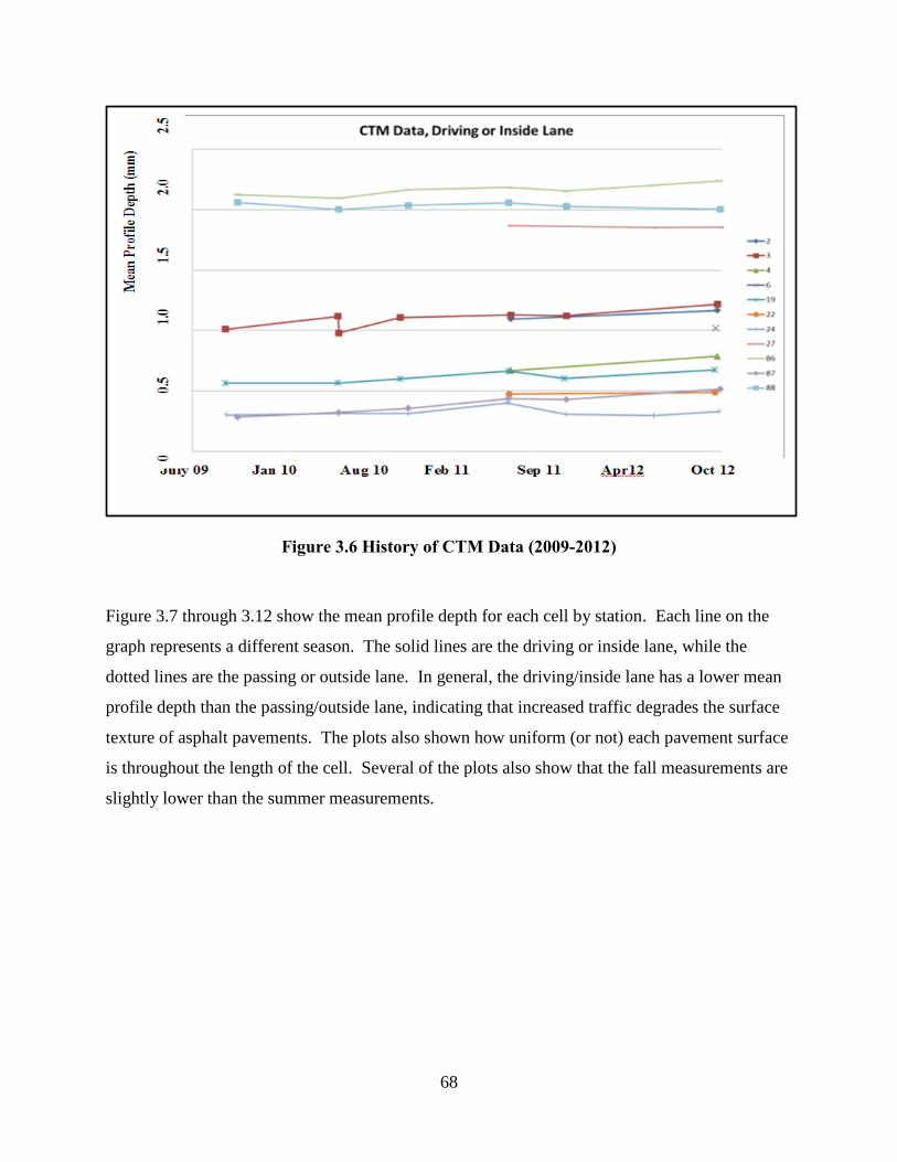
68
Figure 3.6 History of CTM Data (2009-2012)
Figure 3.7 through 3.12 show the mean profile depth for each cell by station. Each line on the
graph represents a different season. The solid lines are the driving or inside lane, while the
dotted lines are the passing or outside lane. In general, the driving/inside lane has a lower mean
profile depth than the passing/outside lane, indicating that increased traffic degrades the surface
texture of asphalt pavements. The plots also shown how uniform (or not) each pavement surface
is throughout the length of the cell. Several of the plots also show that the fall measurements are
slightly lower than the summer measurements.
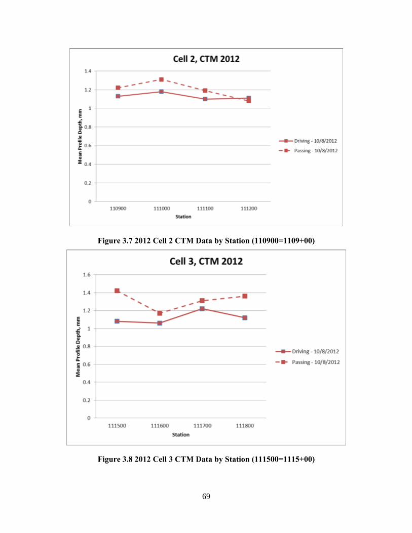
69
Figure 3.7 2012 Cell 2 CTM Data by Station (110900=1109+00)
Figure 3.8 2012 Cell 3 CTM Data by Station (111500=1115+00)
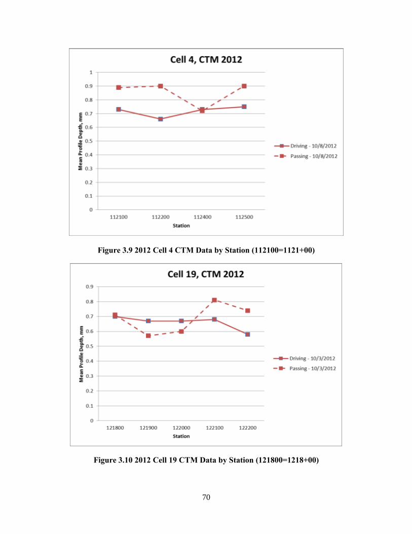
70
Figure 3.9 2012 Cell 4 CTM Data by Station (112100=1121+00)
Figure 3.10 2012 Cell 19 CTM Data by Station (121800=1218+00)
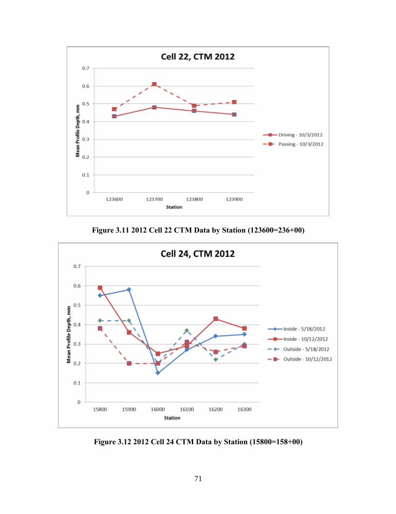
71
Figure 3.11 2012 Cell 22 CTM Data by Station (123600=236+00)
Figure 3.12 2012 Cell 24 CTM Data by Station (15800=158+00)
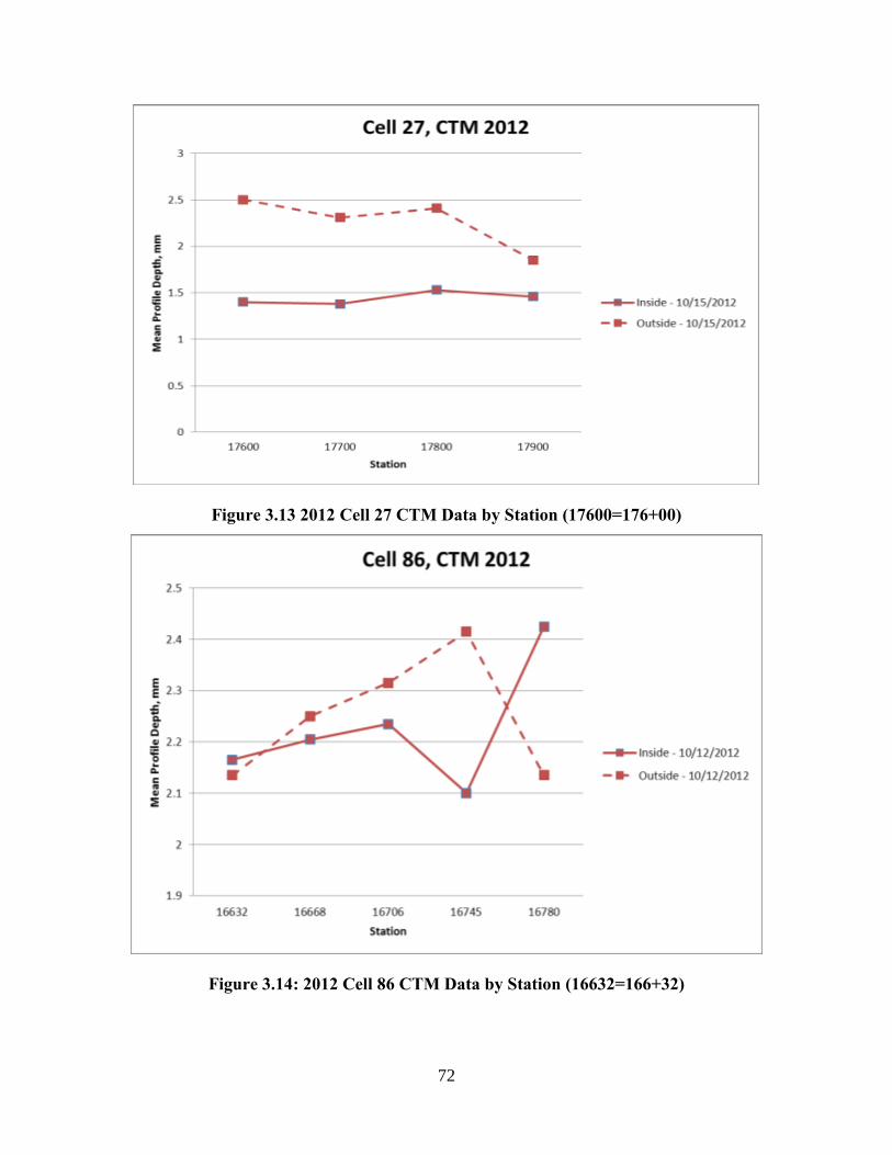
72
Figure 3.13 2012 Cell 27 CTM Data by Station (17600=176+00)
Figure 3.14: 2012 Cell 86 CTM Data by Station (16632=166+32)
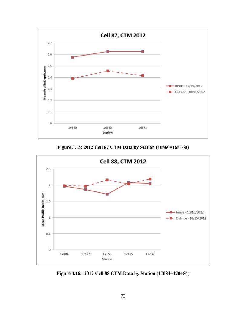
73
Figure 3.15: 2012 Cell 87 CTM Data by Station (16860=168+60)
Figure 3.16: 2012 Cell 88 CTM Data by Station (17084=170+84)
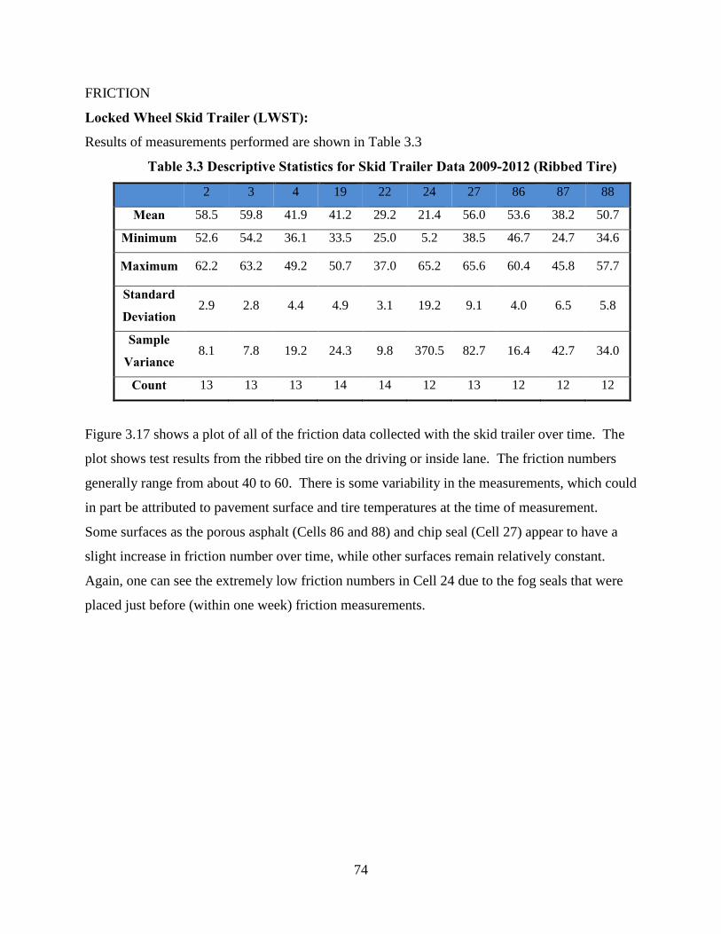
74
FRICTION
Locked Wheel Skid Trailer (LWST): Results of measurements performed are shown in Table 3.3
Table 3.3 Descriptive Statistics for Skid Trailer Data 2009-2012 (Ribbed Tire)
2 3 4 19 22 24 27 86 87 88
Mean 58.5 59.8 41.9 41.2 29.2 21.4 56.0 53.6 38.2 50.7
Minimum 52.6 54.2 36.1 33.5 25.0 5.2 38.5 46.7 24.7 34.6
Maximum 62.2 63.2 49.2 50.7 37.0 65.2 65.6 60.4 45.8 57.7
Standard
Deviation 2.9 2.8 4.4 4.9 3.1 19.2 9.1 4.0 6.5 5.8
Sample
Variance 8.1 7.8 19.2 24.3 9.8 370.5 82.7 16.4 42.7 34.0
Count 13 13 13 14 14 12 13 12 12 12
Figure 3.17 shows a plot of all of the friction data collected with the skid trailer over time. The
plot shows test results from the ribbed tire on the driving or inside lane. The friction numbers
generally range from about 40 to 60. There is some variability in the measurements, which could
in part be attributed to pavement surface and tire temperatures at the time of measurement.
Some surfaces as the porous asphalt (Cells 86 and 88) and chip seal (Cell 27) appear to have a
slight increase in friction number over time, while other surfaces remain relatively constant.
Again, one can see the extremely low friction numbers in Cell 24 due to the fog seals that were
placed just before (within one week) friction measurements.
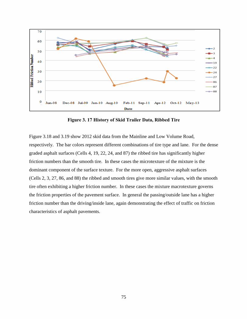
75
Figure 3. 17 History of Skid Trailer Data, Ribbed Tire
Figure 3.18 and 3.19 show 2012 skid data from the Mainline and Low Volume Road,
respectively. The bar colors represent different combinations of tire type and lane. For the dense
graded asphalt surfaces (Cells 4, 19, 22, 24, and 87) the ribbed tire has significantly higher
friction numbers than the smooth tire. In these cases the microtexture of the mixture is the
dominant component of the surface texture. For the more open, aggressive asphalt surfaces
(Cells 2, 3, 27, 86, and 88) the ribbed and smooth tires give more similar values, with the smooth
tire often exhibiting a higher friction number. In these cases the mixture macrotexture governs
the friction properties of the pavement surface. In general the passing/outside lane has a higher
friction number than the driving/inside lane, again demonstrating the effect of traffic on friction
characteristics of asphalt pavements.
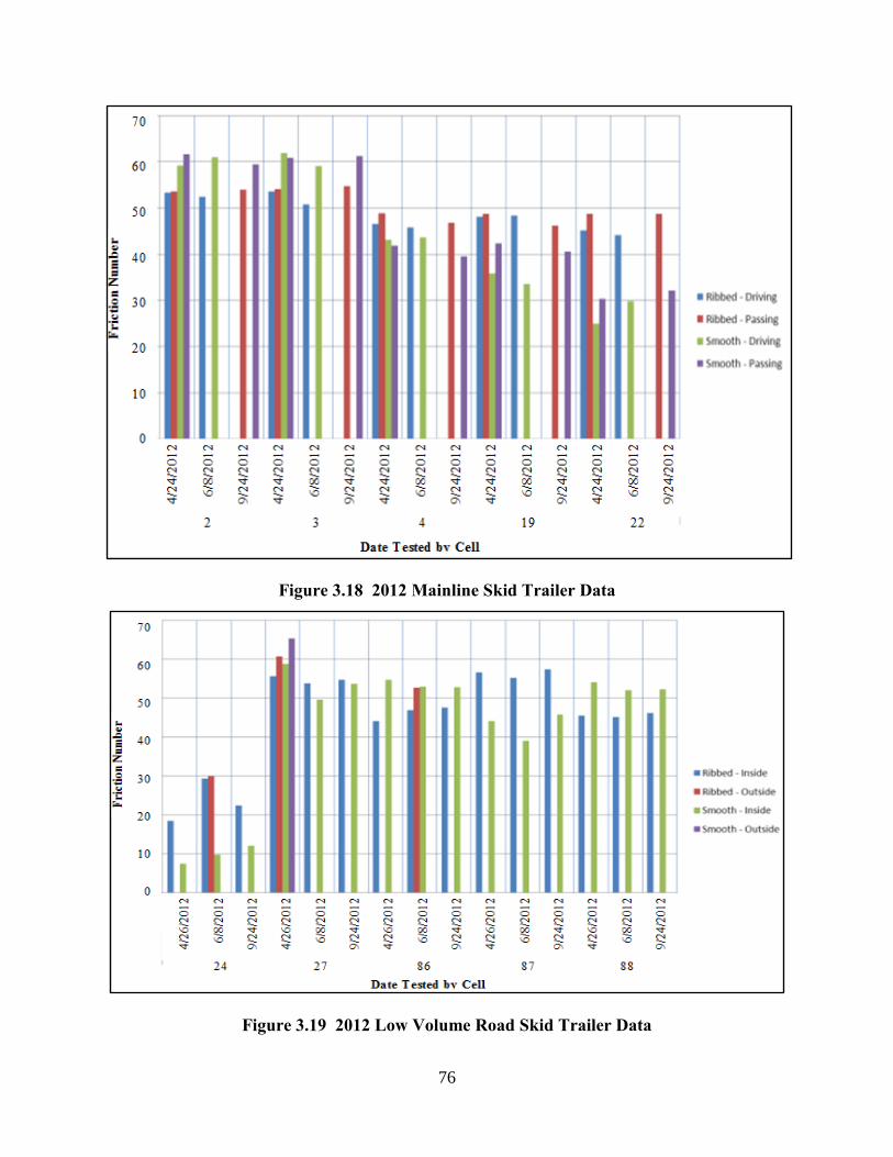
76
Figure 3.18 2012 Mainline Skid Trailer Data
Figure 3.19 2012 Low Volume Road Skid Trailer Data
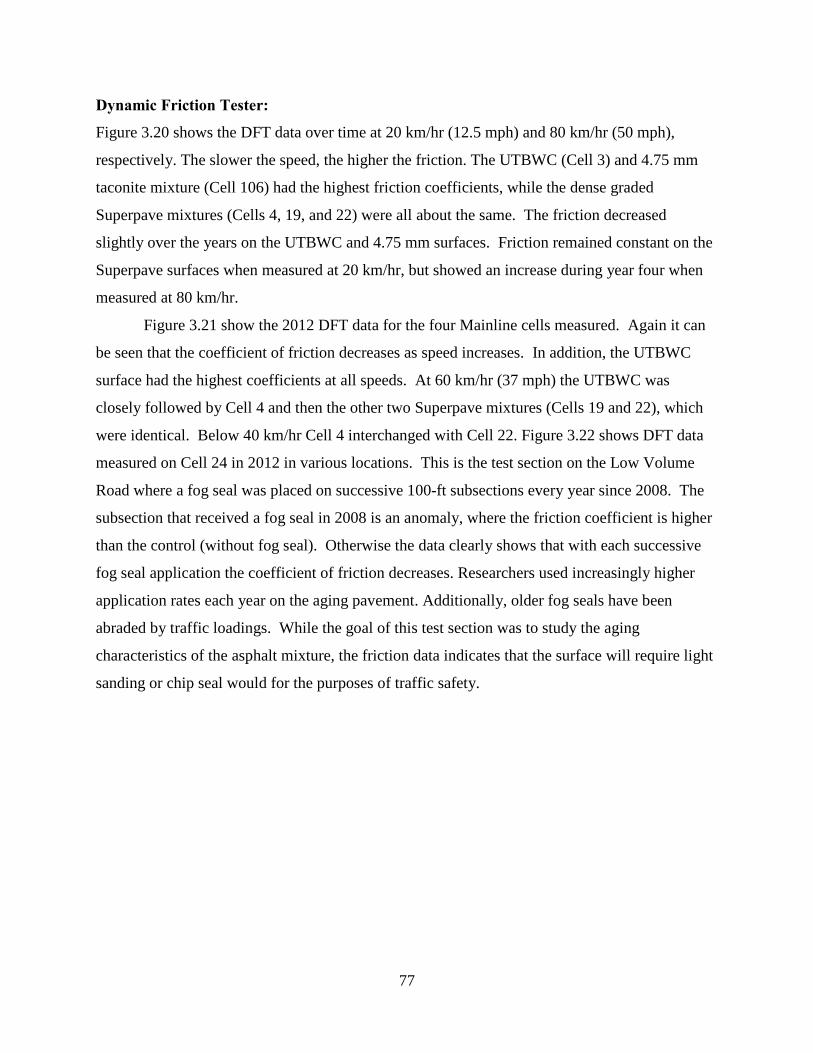
77
Dynamic Friction Tester:
Figure 3.20 shows the DFT data over time at 20 km/hr (12.5 mph) and 80 km/hr (50 mph),
respectively. The slower the speed, the higher the friction. The UTBWC (Cell 3) and 4.75 mm
taconite mixture (Cell 106) had the highest friction coefficients, while the dense graded
Superpave mixtures (Cells 4, 19, and 22) were all about the same. The friction decreased
slightly over the years on the UTBWC and 4.75 mm surfaces. Friction remained constant on the
Superpave surfaces when measured at 20 km/hr, but showed an increase during year four when
measured at 80 km/hr.
Figure 3.21 show the 2012 DFT data for the four Mainline cells measured. Again it can
be seen that the coefficient of friction decreases as speed increases. In addition, the UTBWC
surface had the highest coefficients at all speeds. At 60 km/hr (37 mph) the UTBWC was
closely followed by Cell 4 and then the other two Superpave mixtures (Cells 19 and 22), which
were identical. Below 40 km/hr Cell 4 interchanged with Cell 22. Figure 3.22 shows DFT data
measured on Cell 24 in 2012 in various locations. This is the test section on the Low Volume
Road where a fog seal was placed on successive 100-ft subsections every year since 2008. The
subsection that received a fog seal in 2008 is an anomaly, where the friction coefficient is higher
than the control (without fog seal). Otherwise the data clearly shows that with each successive
fog seal application the coefficient of friction decreases. Researchers used increasingly higher
application rates each year on the aging pavement. Additionally, older fog seals have been
abraded by traffic loadings. While the goal of this test section was to study the aging
characteristics of the asphalt mixture, the friction data indicates that the surface will require light
sanding or chip seal would for the purposes of traffic safety.
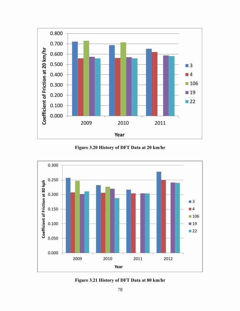
78
Figure 3.20 History of DFT Data at 20 km/hr
0.000
0.100
0.200
0.300
0.400
0.500
0.600
0.700
0.800
2009 2010 2011 2012
Coef
ficie
nt o
f Fric
tion
at 2
0 kp
h
Year
3
4
106
19
22
Figure 3.21 History of DFT Data at 80 km/hr
0.000
0.050
0.100
0.150
0.200
0.250
0.300
2009 2010 2011Coef
ficie
nt o
f Fric
tion
at 8
0 km
/hr
Year
3
4
106
19
22
0.000
0.050
0.100
0.150
0.200
0.250
0.300
2009 2010 2011 2012
Coef
ficie
nt o
f Fric
tion
at 8
0 kp
h
Year
3
4
106
19
22
0.000
0.100
0.200
0.300
0.400
0.500
0.600
0.700
0.800
2009 2010 2011Coef
ficie
nt o
f Fric
tion
at 2
0 km
/hr
Year
3
4
106
19
22
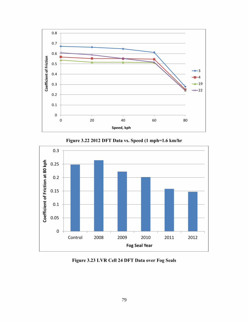
79
Figure 3.22 2012 DFT Data vs. Speed (1 mph=1.6 km/hr
0.000
0.100
0.200
0.300
0.400
0.500
0.600
0.700
0.800
0 20 40 60 80
Coef
ficie
nt o
f Fric
tion
Speed, km/hr
3
4
19
22
Figure 3.23 LVR Cell 24 DFT Data over Fog Seals
0
0.1
0.2
0.3
0.4
0.5
0.6
0.7
0.8
0 20 40 60 80
Coef
ficie
nt o
f Fric
tion
Speed, kph
3
4
19
22
0.000
0.050
0.100
0.150
0.200
0.250
0.300
Control 2008 2009 2010 2011Coef
ficie
nt o
f Fric
tion
at 8
0 km
/hr
Fog Seal Year
0
0.05
0.1
0.15
0.2
0.25
0.3
Control 2008 2009 2010 2011 2012
Coef
ficie
nt o
f Fric
tion
at 8
0 kp
h
Fog Seal Year
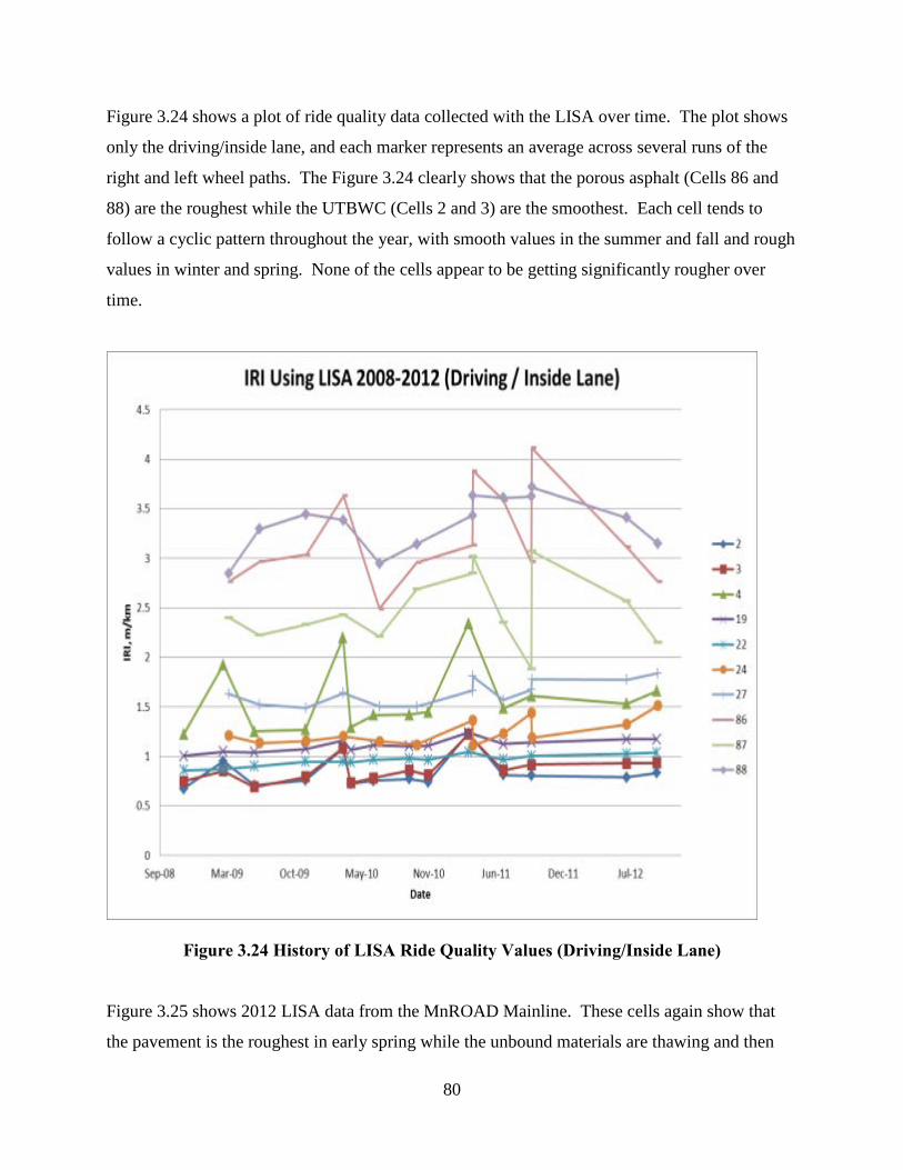
80
Figure 3.24 shows a plot of ride quality data collected with the LISA over time. The plot shows
only the driving/inside lane, and each marker represents an average across several runs of the
right and left wheel paths. The Figure 3.24 clearly shows that the porous asphalt (Cells 86 and
88) are the roughest while the UTBWC (Cells 2 and 3) are the smoothest. Each cell tends to
follow a cyclic pattern throughout the year, with smooth values in the summer and fall and rough
values in winter and spring. None of the cells appear to be getting significantly rougher over
time.
Figure 3.24 History of LISA Ride Quality Values (Driving/Inside Lane)
Figure 3.25 shows 2012 LISA data from the MnROAD Mainline. These cells again show that
the pavement is the roughest in early spring while the unbound materials are thawing and then
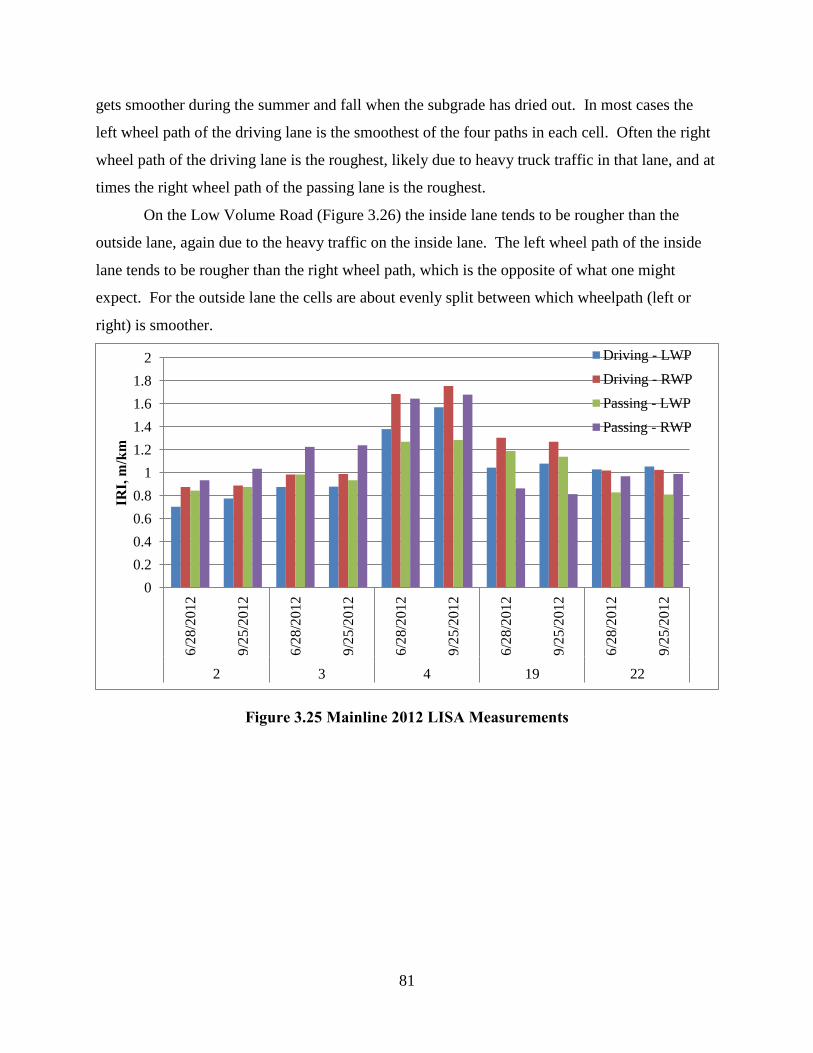
81
gets smoother during the summer and fall when the subgrade has dried out. In most cases the
left wheel path of the driving lane is the smoothest of the four paths in each cell. Often the right
wheel path of the driving lane is the roughest, likely due to heavy truck traffic in that lane, and at
times the right wheel path of the passing lane is the roughest.
On the Low Volume Road (Figure 3.26) the inside lane tends to be rougher than the
outside lane, again due to the heavy traffic on the inside lane. The left wheel path of the inside
lane tends to be rougher than the right wheel path, which is the opposite of what one might
expect. For the outside lane the cells are about evenly split between which wheelpath (left or
right) is smoother.
Figure 3.25 Mainline 2012 LISA Measurements
00.20.40.60.8
11.21.41.61.8
2
6/28
/201
2
9/25
/201
2
6/28
/201
2
9/25
/201
2
6/28
/201
2
9/25
/201
2
6/28
/201
2
9/25
/201
2
6/28
/201
2
9/25
/201
22 3 4 19 22
IRI,
m/k
m
Driving - LWPDriving - RWPPassing - LWPPassing - RWP
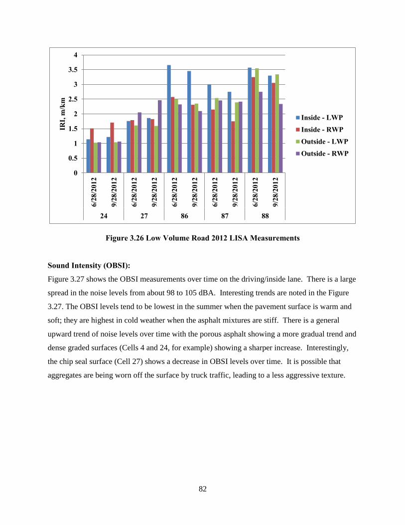
82
Figure 3.26 Low Volume Road 2012 LISA Measurements
0
0.5
1
1.5
2
2.5
3
3.5
4
6/28
/201
2
9/28
/201
2
6/28
/201
2
9/28
/201
2
6/28
/201
2
9/28
/201
2
6/28
/201
2
9/28
/201
2
6/28
/201
2
9/28
/201
2
24 27 86 87 88
IRI,
m/k
m
Inside - LWPInside - RWPOutside - LWPOutside - RWP
Sound Intensity (OBSI):
Figure 3.27 shows the OBSI measurements over time on the driving/inside lane. There is a large
spread in the noise levels from about 98 to 105 dBA. Interesting trends are noted in the Figure
3.27. The OBSI levels tend to be lowest in the summer when the pavement surface is warm and
soft; they are highest in cold weather when the asphalt mixtures are stiff. There is a general
upward trend of noise levels over time with the porous asphalt showing a more gradual trend and
dense graded surfaces (Cells 4 and 24, for example) showing a sharper increase. Interestingly,
the chip seal surface (Cell 27) shows a decrease in OBSI levels over time. It is possible that
aggregates are being worn off the surface by truck traffic, leading to a less aggressive texture.
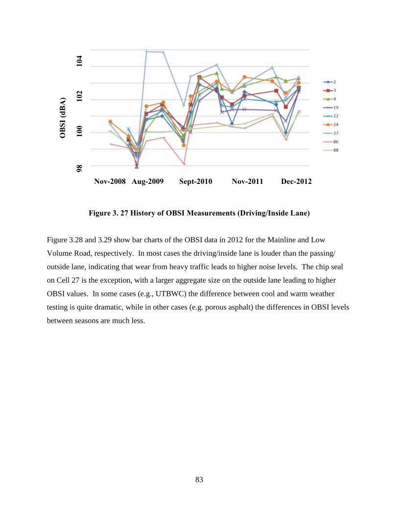
83
Figure 3. 27 History of OBSI Measurements (Driving/Inside Lane)
Nov-2008 Aug-2009 Sept-2010 Nov-2011 Dec-2012
O
BSI (
dBA
)
98
1
00
10
2
104
Figure 3.28 and 3.29 show bar charts of the OBSI data in 2012 for the Mainline and Low
Volume Road, respectively. In most cases the driving/inside lane is louder than the passing/
outside lane, indicating that wear from heavy traffic leads to higher noise levels. The chip seal
on Cell 27 is the exception, with a larger aggregate size on the outside lane leading to higher
OBSI values. In some cases (e.g., UTBWC) the difference between cool and warm weather
testing is quite dramatic, while in other cases (e.g. porous asphalt) the differences in OBSI levels
between seasons are much less.
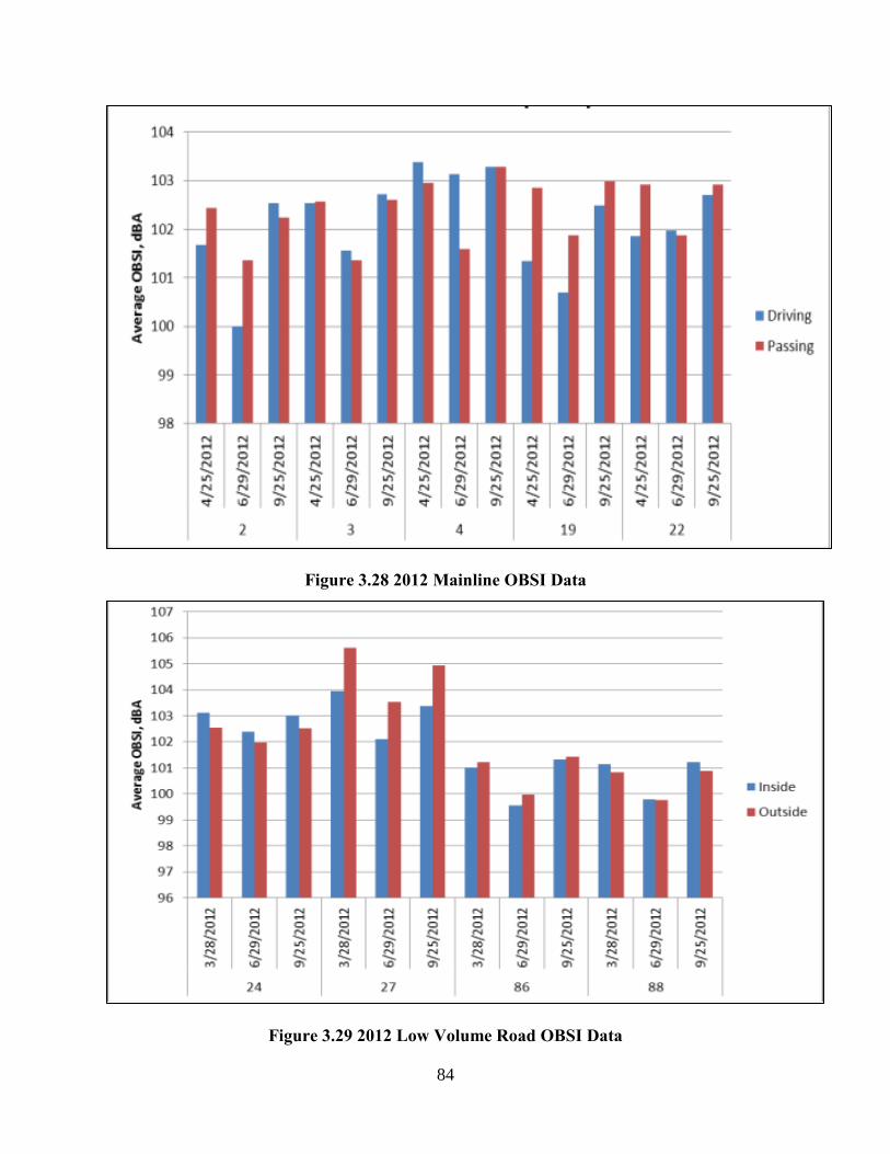
84
Figure 3.28 2012 Mainline OBSI Data
Figure 3.29 2012 Low Volume Road OBSI Data
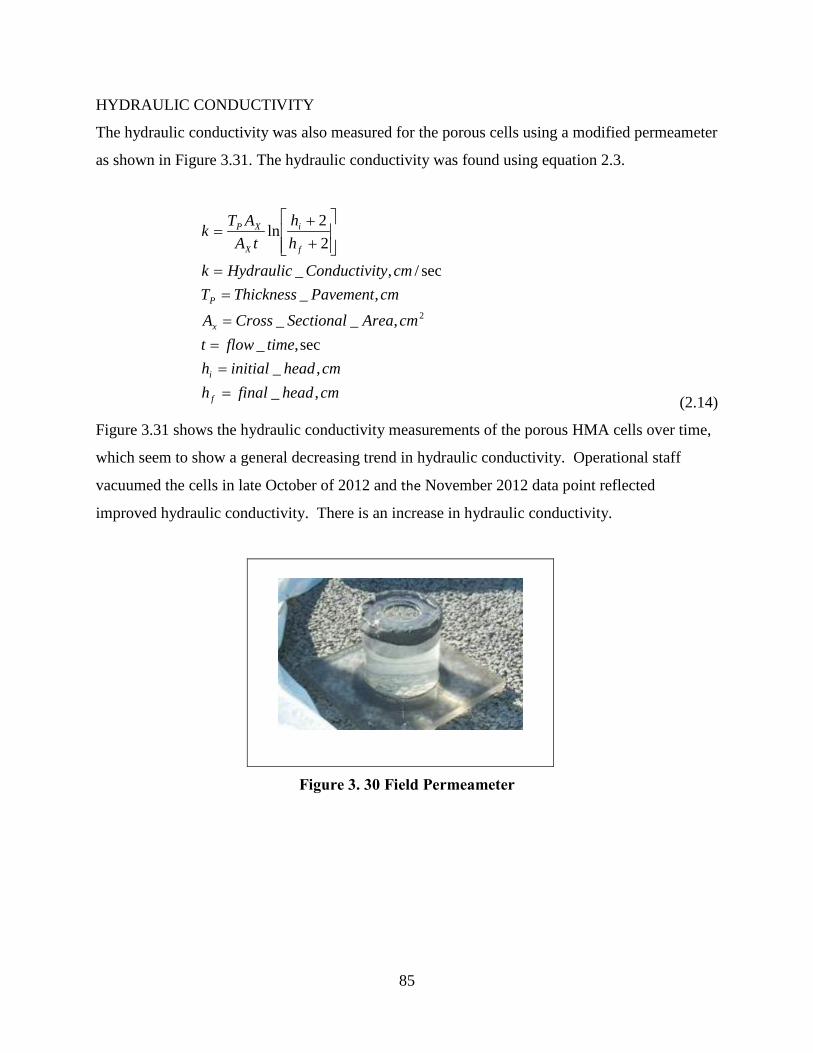
85
HYDRAULIC CONDUCTIVITY
The hydraulic conductivity was also measured for the porous cells using a modified permeameter
as shown in Figure 3.31. The hydraulic conductivity was found using equation 2.3.
cmheadfinalhcmheadinitialh
timeflowtcmAreaSectionalCrossA
cmPavementThicknessTcmtyConductiviHydraulick
hh
tAATk
f
i
x
P
f
i
X
XP
,_,_
sec,_,__
,_sec/,_
22
ln
2
====
==
++
=
(2.14)
Figure 3.31 shows the hydraulic conductivity measurements of the porous HMA cells over time,
which seem to show a general decreasing trend in hydraulic conductivity. Operational staff
vacuumed the cells in late October of 2012 and the November 2012 data point reflected
improved hydraulic conductivity. There is an increase in hydraulic conductivity.
Figure 3. 30 Field Permeameter
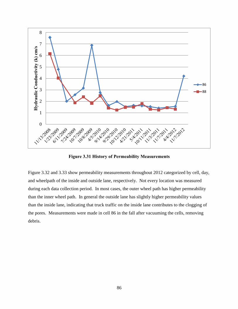
86
Figure 3.31 History of Permeability Measurements
0
1
2
3
4
5
6
7
8H
ydra
ulic
Con
duct
ivity
(k) c
m/s
86
88
Figure 3.32 and 3.33 show permeability measurements throughout 2012 categorized by cell, day,
and wheelpath of the inside and outside lane, respectively. Not every location was measured
during each data collection period. In most cases, the outer wheel path has higher permeability
than the inner wheel path. In general the outside lane has slightly higher permeability values
than the inside lane, indicating that truck traffic on the inside lane contributes to the clogging of
the pores. Measurements were made in cell 86 in the fall after vacuuming the cells, removing
debris.
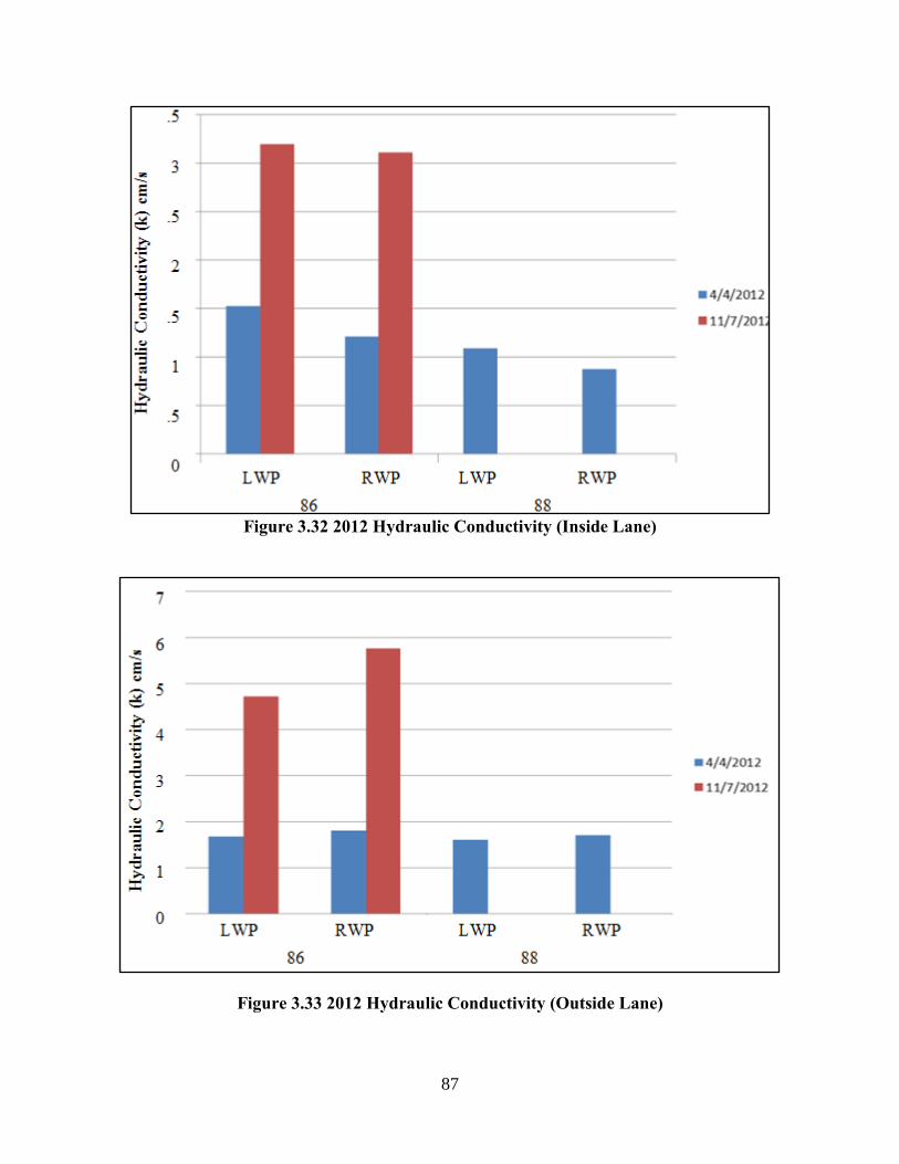
87
Figure 3.32 2012 Hydraulic Conductivity (Inside Lane)
Figure 3.33 2012 Hydraulic Conductivity (Outside Lane)
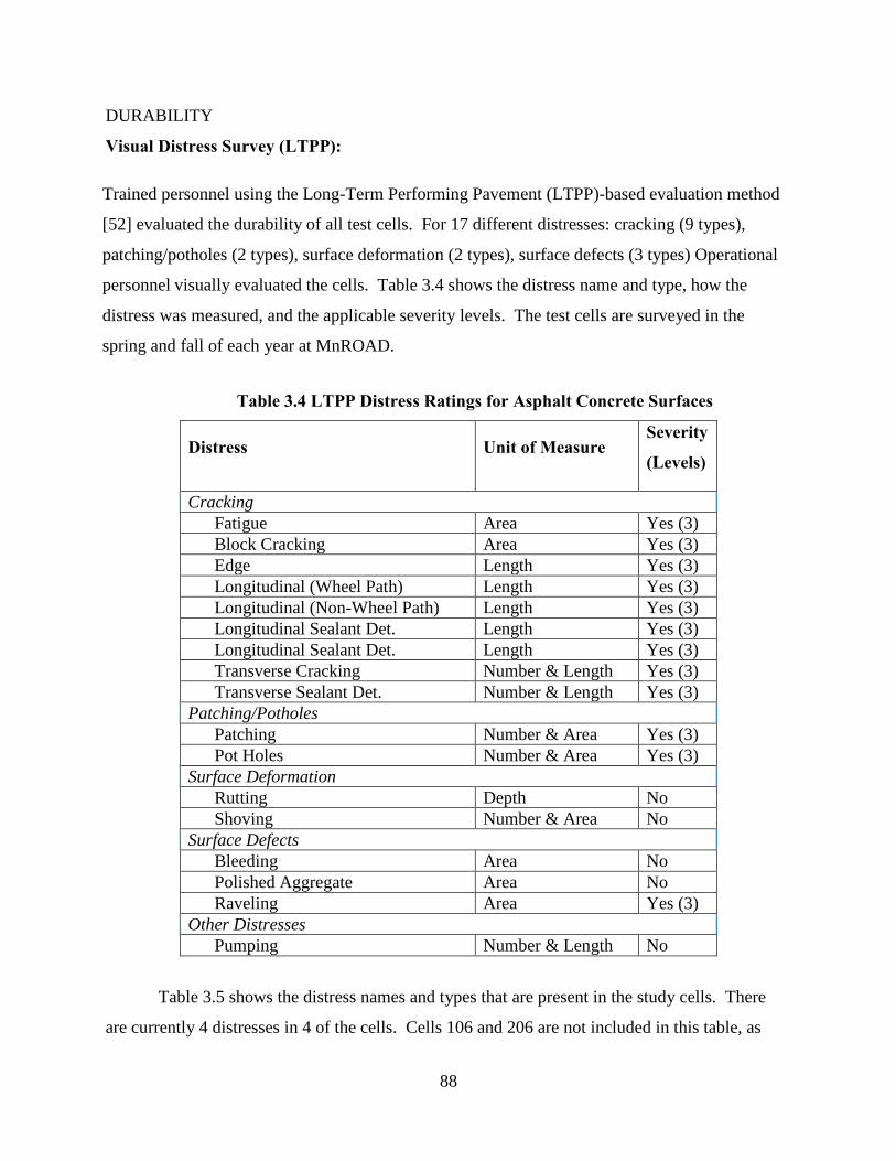
88
DURABILITY
Visual Distress Survey (LTPP):
Trained personnel using the Long-Term Performing Pavement (LTPP)-based evaluation method
[52] evaluated the durability of all test cells. For 17 different distresses: cracking (9 types),
patching/potholes (2 types), surface deformation (2 types), surface defects (3 types) Operational
personnel visually evaluated the cells. Table 3.4 shows the distress name and type, how the
distress was measured, and the applicable severity levels. The test cells are surveyed in the
spring and fall of each year at MnROAD.
Table 3.4 LTPP Distress Ratings for Asphalt Concrete Surfaces
Distress Unit of Measure Severity
(Levels)
Cracking Fatigue Area Yes (3) Block Cracking Area Yes (3) Edge Length Yes (3) Longitudinal (Wheel Path) Length Yes (3) Longitudinal (Non-Wheel Path) Length Yes (3) Longitudinal Sealant Det.
Length Yes (3) Longitudinal Sealant Det.
Length Yes (3) Transverse Cracking Number & Length Yes (3) Transverse Sealant Det. Number & Length Yes (3)
Patching/Potholes Patching Number & Area Yes (3) Pot Holes Number & Area Yes (3)
Surface Deformation Rutting Depth No Shoving Number & Area No
Surface Defects Bleeding Area No Polished Aggregate Area No Raveling Area Yes (3)
Other Distresses Pumping Number & Length No
Table 3.5 shows the distress names and types that are present in the study cells. There
are currently 4 distresses in 4 of the cells. Cells 106 and 206 are not included in this table, as
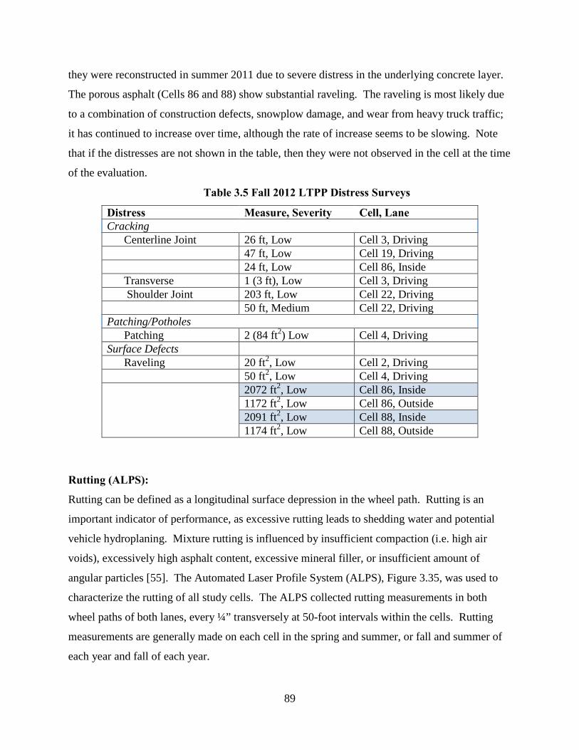
89
they were reconstructed in summer 2011 due to severe distress in the underlying concrete layer.
The porous asphalt (Cells 86 and 88) show substantial raveling. The raveling is most likely due
to a combination of construction defects, snowplow damage, and wear from heavy truck traffic;
it has continued to increase over time, although the rate of increase seems to be slowing. Note
that if the distresses are not shown in the table, then they were not observed in the cell at the time
of the evaluation.
Table 3.5 Fall 2012 LTPP Distress Surveys
Distress Measure, Severity Cell, Lane Cracking
Centerline Joint 26 ft, Low Cell 3, Driving 47 ft, Low Cell 19, Driving 24 ft, Low Cell 86, Inside Transverse 1 (3 ft), Low Cell 3, Driving
Shoulder Joint 203 ft, Low Cell 22, Driving 50 ft, Medium Cell 22, Driving Patching/Potholes
Patching 2 (84 ft2) Low Cell 4, Driving Surface Defects
Raveling 20 ft2, Low Cell 2, Driving 50 ft2, Low Cell 4, Driving 2072 ft2, Low Cell 86, Inside
1172 ft2, Low Cell 86, Outside 2091 ft2, Low Cell 88, Inside 1174 ft2, Low Cell 88, Outside
Rutting (ALPS): Rutting can be defined as a longitudinal surface depression in the wheel path. Rutting is an
important indicator of performance, as excessive rutting leads to shedding water and potential
vehicle hydroplaning. Mixture rutting is influenced by insufficient compaction (i.e. high air
voids), excessively high asphalt content, excessive mineral filler, or insufficient amount of
angular particles [55]. The Automated Laser Profile System (ALPS), Figure 3.35, was used to
characterize the rutting of all study cells. The ALPS collected rutting measurements in both
wheel paths of both lanes, every ¼” transversely at 50-foot intervals within the cells. Rutting
measurements are generally made on each cell in the spring and summer, or fall and summer of
each year and fall of each year.
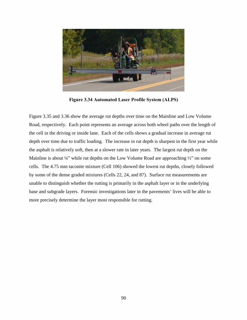
90
Figure 3.34 Automated Laser Profile System (ALPS)
Figure 3.35 and 3.36 show the average rut depths over time on the Mainline and Low Volume
Road, respectively. Each point represents an average across both wheel paths over the length of
the cell in the driving or inside lane. Each of the cells shows a gradual increase in average rut
depth over time due to traffic loading. The increase in rut depth is sharpest in the first year while
the asphalt is relatively soft, then at a slower rate in later years. The largest rut depth on the
Mainline is about ¼” while rut depths on the Low Volume Road are approaching ½” on some
cells. The 4.75 mm taconite mixture (Cell 106) showed the lowest rut depths, closely followed
by some of the dense graded mixtures (Cells 22, 24, and 87). Surface rut measurements are
unable to distinguish whether the rutting is primarily in the asphalt layer or in the underlying
base and subgrade layers. Forensic investigations later in the pavements’ lives will be able to
more precisely determine the layer most responsible for rutting.
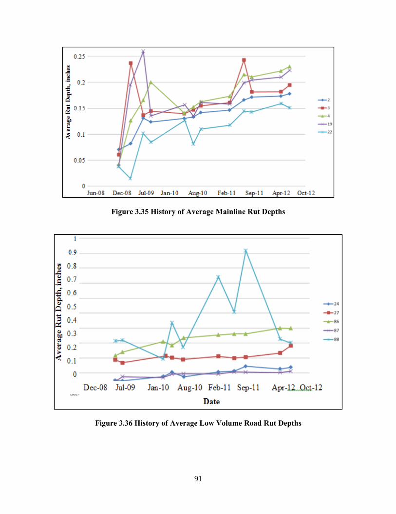
91
Figure 3.35 History of Average Mainline Rut Depths
Figure 3.36 History of Average Low Volume Road Rut Depths
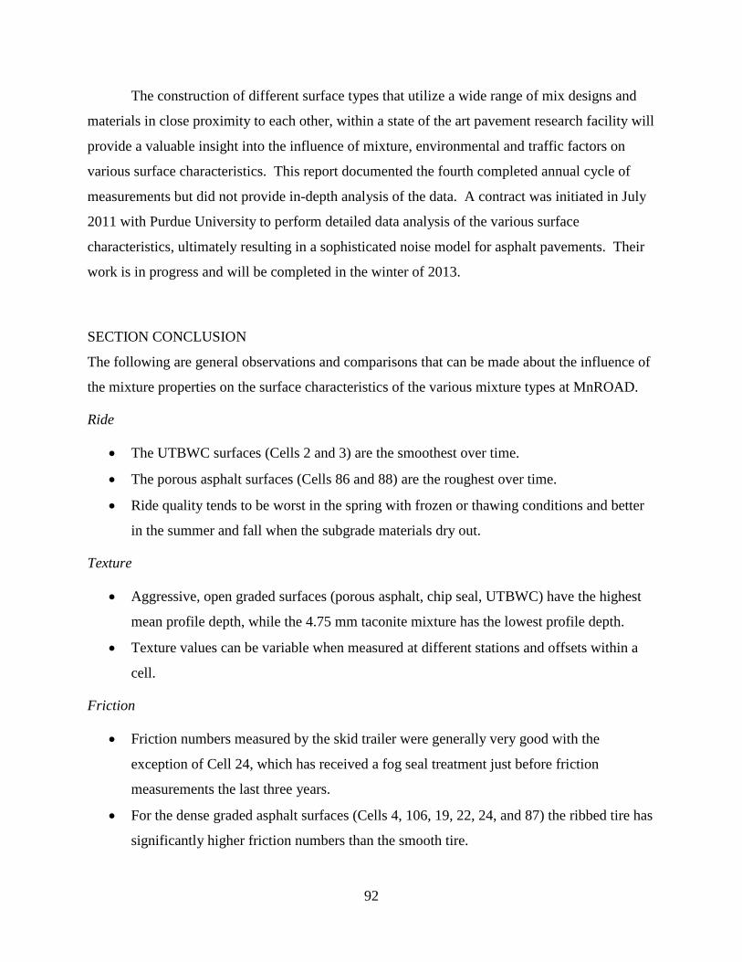
92
The construction of different surface types that utilize a wide range of mix designs and
materials in close proximity to each other, within a state of the art pavement research facility will
provide a valuable insight into the influence of mixture, environmental and traffic factors on
various surface characteristics. This report documented the fourth completed annual cycle of
measurements but did not provide in-depth analysis of the data. A contract was initiated in July
2011 with Purdue University to perform detailed data analysis of the various surface
characteristics, ultimately resulting in a sophisticated noise model for asphalt pavements. Their
work is in progress and will be completed in the winter of 2013.
SECTION CONCLUSION
The following are general observations and comparisons that can be made about the influence of
the mixture properties on the surface characteristics of the various mixture types at MnROAD.
Ride
• The UTBWC surfaces (Cells 2 and 3) are the smoothest over time.
• The porous asphalt surfaces (Cells 86 and 88) are the roughest over time.
• Ride quality tends to be worst in the spring with frozen or thawing conditions and better
in the summer and fall when the subgrade materials dry out.
Texture
• Aggressive, open graded surfaces (porous asphalt, chip seal, UTBWC) have the highest
mean profile depth, while the 4.75 mm taconite mixture has the lowest profile depth.
• Texture values can be variable when measured at different stations and offsets within a
cell.
Friction
• Friction numbers measured by the skid trailer were generally very good with the
exception of Cell 24, which has received a fog seal treatment just before friction
measurements the last three years.
• For the dense graded asphalt surfaces (Cells 4, 106, 19, 22, 24, and 87) the ribbed tire has
significantly higher friction numbers than the smooth tire.

93
• For the more open, aggressive asphalt surfaces (Cells 2, 3, 27, 86, and 88) the ribbed and
smooth tires give more similar values, with the smooth tire often exhibiting a higher
friction number.
• In general the passing/outside lane has a higher friction number than the driving/inside
lane, showing the effect of traffic on friction.
• The UTBWC (Cell 3) and 4.75 mm taconite (Cell 106) surfaces had the highest
coefficient of friction values measured with the dynamic friction tester. The dense
graded Superpave surfaces (Cells 4, 19, and 22) had approximately equal coefficients.
• On Cell 24 the coefficient of friction decreased with each successive application of fog
seal, indicating that a light sanding or chip seal may be considered to maintain a safe
driving surface.
Noise
• The porous asphalt surfaces (Cells 86 and 88) are the quietest, while the chip seal (Cell
27) and some of the dense graded asphalt mixtures (Cells 4 and 24) are the loudest.
• OBSI levels are lowest in the summer when the pavement surface is warm; they are
highest in cold weather.
• There is a general upward trend of noise levels over time with the porous asphalt showing
a more gradual trend and dense graded surfaces showing a sharper increase.
• In some cases (e.g., novachip) the difference between cool and warm weather test results
were significant, while in other cases (e.g. porous asphalt) the differences in OBSI levels
between seasons are much less.
• Porous asphalt surfaces (Cells 86 and 88) have the highest sound absorption coefficients;
UTBWC surfaces (Cells 2 and 3) are a distant second.
• Dense graded asphalt mixtures have extremely low sound absorption coefficients, with
the 4.75 mm taconite mixture (Cell 106) having the lowest.
• The sound absorption coefficients of the open graded surface textures (porous and
UTBWC) decrease significantly over time, while this is not the case for the dense graded
mixtures.
Durability
• The porous asphalt mixtures (Cells 86 and 88) show a substantial amount of raveling,

94
which is most likely due to a combination of construction defects, snowplow damage,
and wear from heavy truck traffic.
• The largest rut depth on the Mainline is about ¼” while rut depths on the Low Volume
Road are approaching ½” on some cells.
• The 4.75 mm taconite mixture (Cell 106) showed the lowest rut depths, closely followed
by some of the dense graded mixtures (Cells 22, 24, and 87).
• The porous asphalt surfaces show the greatest rut depths.

95
CHAPTER 4
ADVANCED DATA ANALYSIS
96
BACKGROUND Major analyses carried out in the study of flexible pavement surfaces include effects of texture
skewness (a measure of the spikiness of the textured surface asperities), temperature and friction.
Section one investigates if skewness compared to mean profile depth is a better indicator or
predictor of Tire-Pavement-Interaction-Noise; section two is to observe the relationship between
temperature and on-board sound intensity; and lastly section three is to observe frictional
properties on asphalt pavements.
Section two discusses the relationship between pavement noise and temperature in
asphalt pavements. In this study, temperature effect was studied with the data obtained from
routine measurements as well as certain decays when OBSI was measured every hour in all the
test cells. Section three discusses frictional properties of tire-pavement interaction in asphalt
pavement surfaces. Friction is essential in pavement infrastructure as a primary indicator of skid
resistance or safety. The data used in the analysis originated from multiple MnROAD asphalt test
cells. This chapter reveals a significant degree of sensitivity of flexible pavements to temperature
and shows the significance of spikiness. It also validated the theorem that friction degradation
follows a pattern of decay, similar to the half-life equation. The rate of friction degradation is
proportional to the value of the friction number.
EVALUATION OF SKEWNESS PROPERTIES SURFACES Many authorities including Izevbekhai [58] discuss the relationship between road texture and
pavement noise. In these articles, they suggest that road texture may have influence on pavement
noise. Most pavement surfaces that have similar mean profile depth do not necessarily have
similar sound intensity. Therefore, researchers are still searching for alternative measures that
can more accurately predict pavement noise. In this project, skewness is investigated under an
assumption that it may be a better approach in predicting the pavement noise than mean profile
depth. Izevbekhai et al [58] showed that texture orientation (spikiness) another term for skewness
was a significant variable in the prediction of Tire-Pavement-Interaction-Noise. The dependent
variable of pavement noise is chosen because it is determined to be the most texture intensive
component of the surface properties. Other measures such as IRI are affected more by the
condition of the pavement structure than the surface textures.
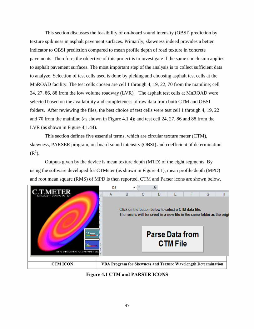
97
This section discusses the feasibility of on-board sound intensity (OBSI) prediction by
texture spikiness in asphalt pavement surfaces. Primarily, skewness indeed provides a better
indicator to OBSI prediction compared to mean profile depth of road texture in concrete
pavements. Therefore, the objective of this project is to investigate if the same conclusion applies
to asphalt pavement surfaces. The most important step of the analysis is to collect sufficient data
to analyze. Selection of test cells used is done by picking and choosing asphalt test cells at the
MnROAD facility. The test cells chosen are cell 1 through 4, 19, 22, 70 from the mainline; cell
24, 27, 86, 88 from the low volume roadway (LVR). The asphalt test cells at MnROAD were
selected based on the availability and completeness of raw data from both CTM and OBSI
folders. After reviewing the files, the best choice of test cells were test cell 1 through 4, 19, 22
and 70 from the mainline (as shown in Figure 4.1.4); and test cell 24, 27, 86 and 88 from the
LVR (as shown in Figure 4.1.44).
This section defines five essential terms, which are circular texture meter (CTM),
skewness, PARSER program, on-board sound intensity (OBSI) and coefficient of determination
(R2).
Outputs given by the device is mean texture depth (MTD) of the eight segments. By
using the software developed for CTMeter (as shown in Figure 4.1), mean profile depth (MPD)
and root mean square (RMS) of MPD is then reported. CTM and Parser icons are shown below.
Figure 4.1 CTM and PARSER ICONS CTM ICON VBA Program for Skewness and Texture Wavelength Determination
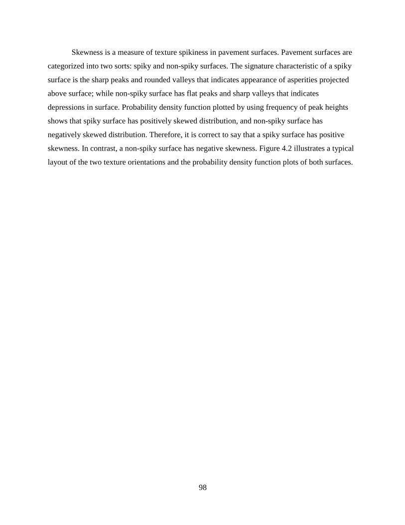
98
Skewness is a measure of texture spikiness in pavement surfaces. Pavement surfaces are
categorized into two sorts: spiky and non-spiky surfaces. The signature characteristic of a spiky
surface is the sharp peaks and rounded valleys that indicates appearance of asperities projected
above surface; while non-spiky surface has flat peaks and sharp valleys that indicates
depressions in surface. Probability density function plotted by using frequency of peak heights
shows that spiky surface has positively skewed distribution, and non-spiky surface has
negatively skewed distribution. Therefore, it is correct to say that a spiky surface has positive
skewness. In contrast, a non-spiky surface has negative skewness. Figure 4.2 illustrates a typical
layout of the two texture orientations and the probability density function plots of both surfaces.
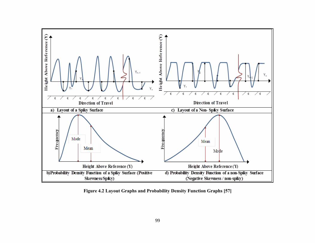
99
Figure 4.2 Layout Graphs and Probability Density Function Graphs [57]
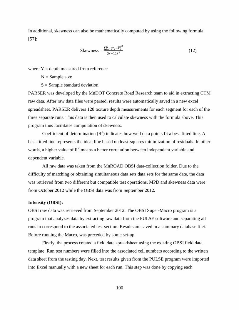
100
In additional, skewness can also be mathematically computed by using the following formula
[57]:
∑ (𝑌 −𝑌)���3
(𝑁−1)𝑆 (12) Skewness =
where Y = depth measured from reference
N = Sample size
S = Sample standard deviation
PARSER was developed by the MnDOT Concrete Road Research team to aid in extracting CTM
raw data. After raw data files were parsed, results were automatically saved in a new excel
spreadsheet. PARSER delivers 128 texture depth measurements for each segment for each of the
three separate runs. This data is then used to calculate skewness with the formula above. This
program thus facilitates computation of skewness.
Coefficient of determination (R2) indicates how well data points fit a best-fitted line. A
best-fitted line represents the ideal line based on least-squares minimization of residuals. In other
words, a higher value of R2 means a better correlation between independent variable and
dependent variable.
All raw data was taken from the MnROAD OBSI data-collection folder. Due to the
difficulty of matching or obtaining simultaneous data sets data sets for the same date, the data
was retrieved from two different but compatible test operations. MPD and skewness data were
from October 2012 while the OBSI data was from September 2012.
𝑖𝑁𝑖=1
3
Intensity (OBSI):
OBSI raw data was retrieved from September 2012. The OBSI Super-Macro program is a
program that analyzes data by extracting raw data from the PULSE software and separating all
runs to correspond to the associated test section. Results are saved in a summary database filet.
Before running the Macro, was preceded by some set-up.
Firstly, the process created a field data spreadsheet using the existing OBSI field data
template. Run test numbers were filled into the associated cell numbers according to the written
data sheet from the testing day. Next, test results given from the PULSE program were imported
into Excel manually with a new sheet for each run. This step was done by copying each
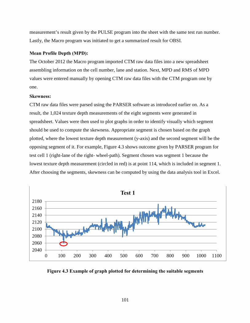
101
measurement’s result given by the PULSE program into the sheet with the same test run number.
Lastly, the Macro program was initiated to get a summarized result for OBSI.
Mean Profile Depth (MPD):
The October 2012 the Macro program imported CTM raw data files into a new spreadsheet
assembling information on the cell number, lane and station. Next, MPD and RMS of MPD
values were entered manually by opening CTM raw data files with the CTM program one by
one.
Skewness:
CTM raw data files were parsed using the PARSER software as introduced earlier on. As a
result, the 1,024 texture depth measurements of the eight segments were generated in
spreadsheet. Values were then used to plot graphs in order to identify visually which segment
should be used to compute the skewness. Appropriate segment is chosen based on the graph
plotted, where the lowest texture depth measurement (y-axis) and the second segment will be the
opposing segment of it. For example, Figure 4.3 shows outcome given by PARSER program for
test cell 1 (right-lane of the right- wheel-path). Segment chosen was segment 1 because the
lowest texture depth measurement (circled in red) is at point 114, which is included in segment 1.
After choosing the segments, skewness can be computed by using the data analysis tool in Excel.
Figure 4.3 Example of graph plotted for determining the suitable segments
20402060208021002120214021602180
0 100 200 300 400 500 600 700 800 900 1000 1100
Test 1
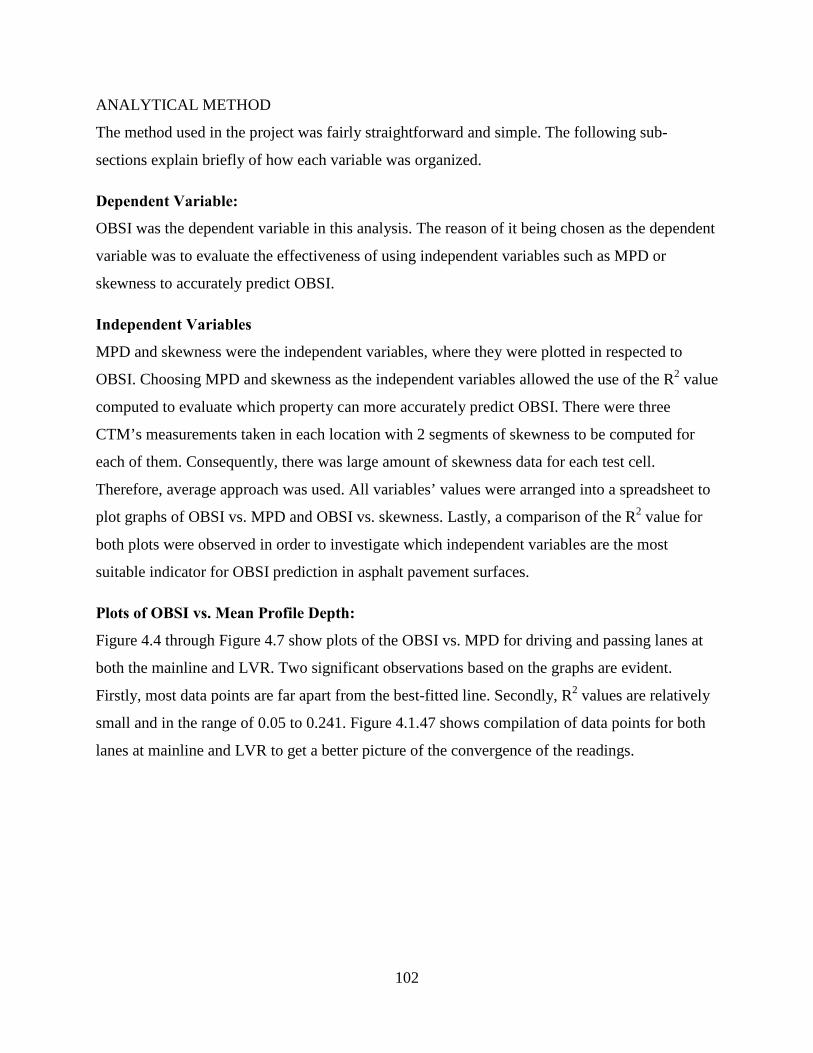
102
ANALYTICAL METHOD
The method used in the project was fairly straightforward and simple. The following sub-
sections explain briefly of how each variable was organized.
Dependent Variable:
OBSI was the dependent variable in this analysis. The reason of it being chosen as the dependent
variable was to evaluate the effectiveness of using independent variables such as MPD or
skewness to accurately predict OBSI.
Independent Variables
MPD and skewness were the independent variables, where they were plotted in respected to
OBSI. Choosing MPD and skewness as the independent variables allowed the use of the R2 value
computed to evaluate which property can more accurately predict OBSI. There were three
CTM’s measurements taken in each location with 2 segments of skewness to be computed for
each of them. Consequently, there was large amount of skewness data for each test cell.
Therefore, average approach was used. All variables’ values were arranged into a spreadsheet to
plot graphs of OBSI vs. MPD and OBSI vs. skewness. Lastly, a comparison of the R2 value for
both plots were observed in order to investigate which independent variables are the most
suitable indicator for OBSI prediction in asphalt pavement surfaces.
Plots of OBSI vs. Mean Profile Depth:
Figure 4.4 through Figure 4.7 show plots of the OBSI vs. MPD for driving and passing lanes at
both the mainline and LVR. Two significant observations based on the graphs are evident.
Firstly, most data points are far apart from the best-fitted line. Secondly, R2 values are relatively
small and in the range of 0.05 to 0.241. Figure 4.1.47 shows compilation of data points for both
lanes at mainline and LVR to get a better picture of the convergence of the readings.
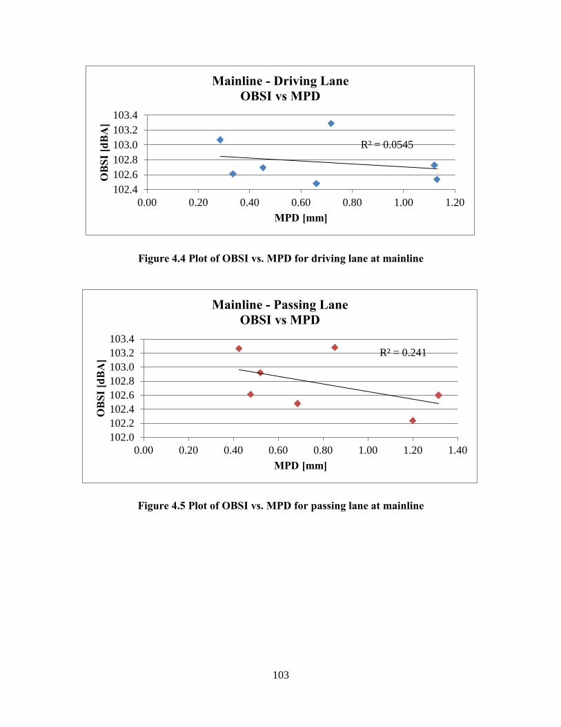
103
Figure 4.4 Plot of OBSI vs. MPD for driving lane at mainline
R² = 0.0545
102.4102.6102.8103.0103.2103.4
0.00 0.20 0.40 0.60 0.80 1.00 1.20
OB
SI [d
BA
]
MPD [mm]
Mainline - Driving Lane OBSI vs MPD
Figure 4.5 Plot of OBSI vs. MPD for passing lane at mainline
R² = 0.241
102.0102.2102.4102.6102.8103.0103.2103.4
0.00 0.20 0.40 0.60 0.80 1.00 1.20 1.40
OB
SI [d
BA
]
MPD [mm]
Mainline - Passing Lane OBSI vs MPD
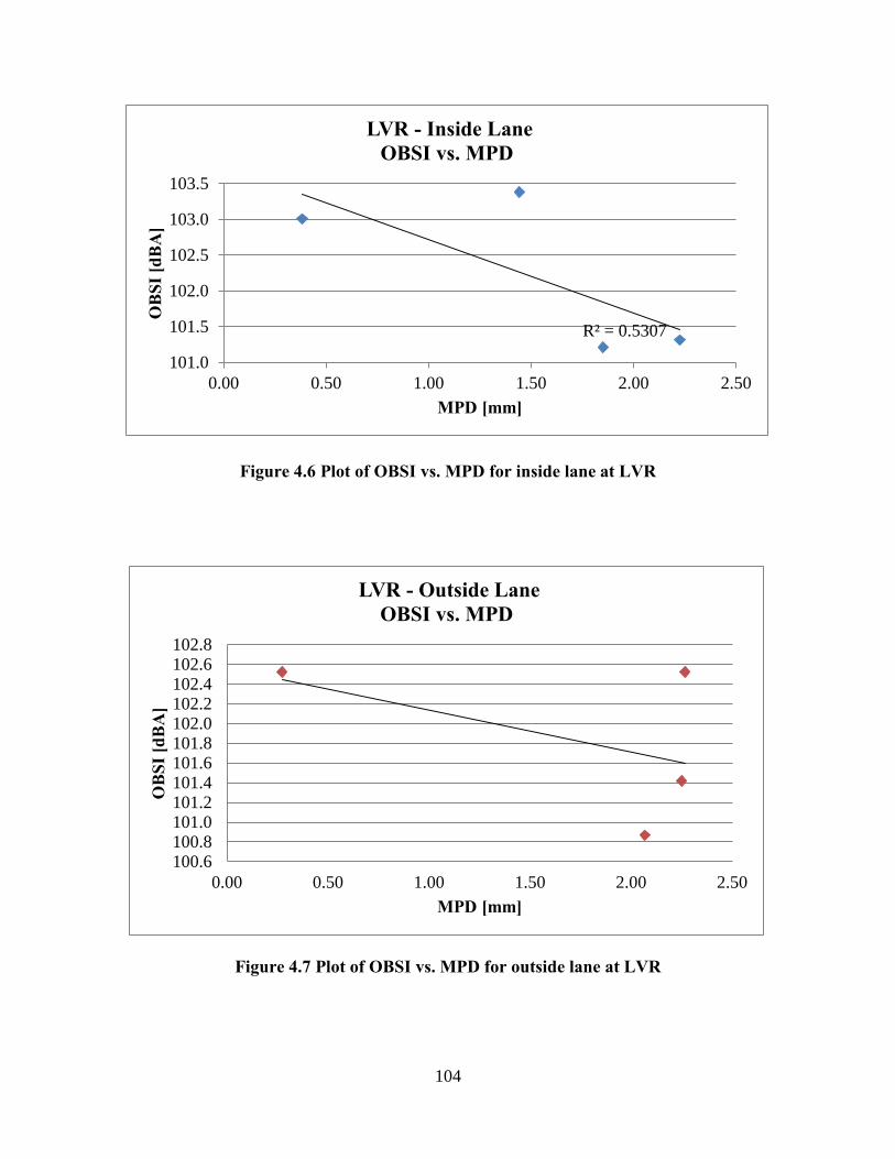
104
Figure 4.6 Plot of OBSI vs. MPD for inside lane at LVR
R² = 0.5307
101.0
101.5
102.0
102.5
103.0
103.5
0.00 0.50 1.00 1.50 2.00 2.50
OB
SI [d
BA
]
MPD [mm]
LVR - Inside Lane OBSI vs. MPD
Figure 4.7 Plot of OBSI vs. MPD for outside lane at LVR
100.6100.8101.0101.2101.4101.6101.8102.0102.2102.4102.6102.8
0.00 0.50 1.00 1.50 2.00 2.50
OB
SI [d
BA
]
MPD [mm]
LVR - Outside Lane OBSI vs. MPD
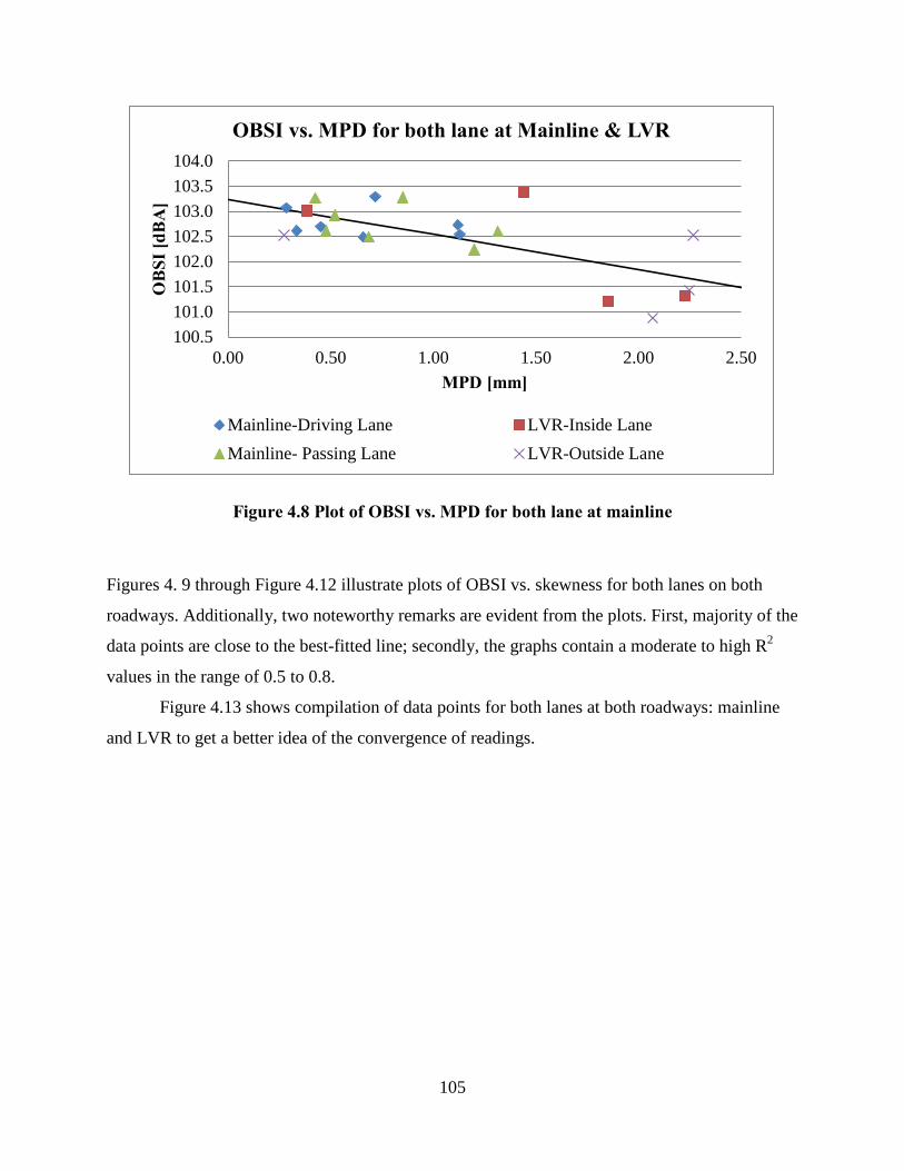
105
Figure 4.8 Plot of OBSI vs. MPD for both lane at mainline
100.5101.0101.5102.0102.5103.0103.5104.0
0.00 0.50 1.00 1.50 2.00 2.50
OB
SI [d
BA
]
MPD [mm]
OBSI vs. MPD for both lane at Mainline & LVR
Mainline-Driving Lane LVR-Inside LaneMainline- Passing Lane LVR-Outside Lane
Figures 4. 9 through Figure 4.12 illustrate plots of OBSI vs. skewness for both lanes on both
roadways. Additionally, two noteworthy remarks are evident from the plots. First, majority of the
data points are close to the best-fitted line; secondly, the graphs contain a moderate to high R2
values in the range of 0.5 to 0.8.
Figure 4.13 shows compilation of data points for both lanes at both roadways: mainline
and LVR to get a better idea of the convergence of readings.
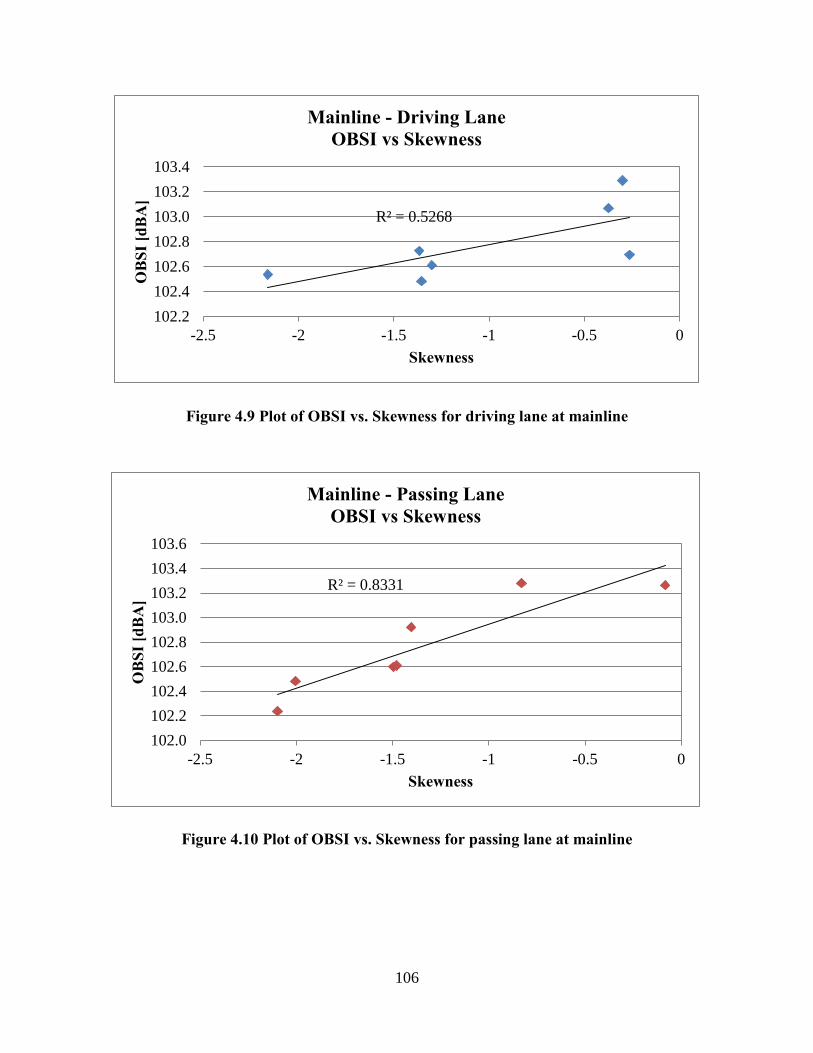
106
Figure 4.9 Plot of OBSI vs. Skewness for driving lane at mainline
R² = 0.5268
102.2102.4102.6102.8103.0103.2103.4
-2.5 -2 -1.5 -1 -0.5 0
OB
SI [d
BA
]
Skewness
Mainline - Driving Lane OBSI vs Skewness
Figure 4.10 Plot of OBSI vs. Skewness for passing lane at mainline
R² = 0.8331
102.0102.2102.4102.6102.8103.0103.2103.4103.6
-2.5 -2 -1.5 -1 -0.5 0
OB
SI [d
BA
]
Skewness
Mainline - Passing Lane OBSI vs Skewness
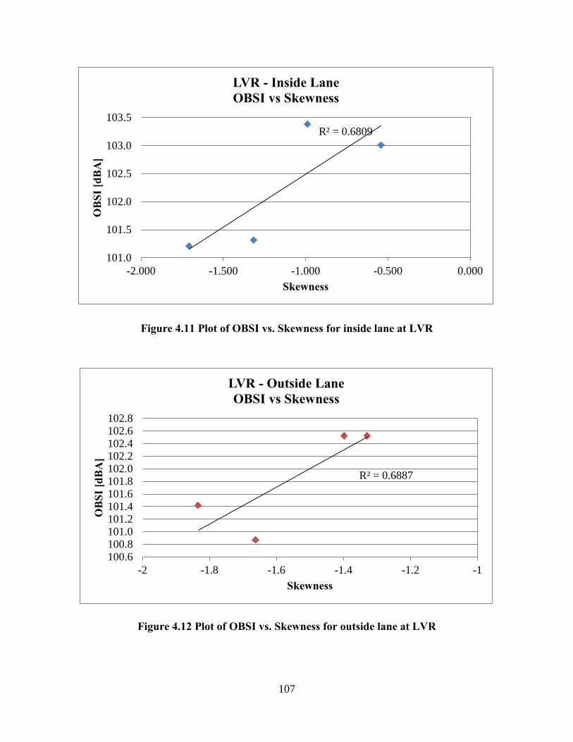
107
Figure 4.11 Plot of OBSI vs. Skewness for inside lane at LVR
R² = 0.6809
101.0
101.5
102.0
102.5
103.0
103.5
-2.000 -1.500 -1.000 -0.500 0.000
OB
SI [d
BA
]
Skewness
LVR - Inside Lane OBSI vs Skewness
Figure 4.12 Plot of OBSI vs. Skewness for outside lane at LVR
R² = 0.6887
100.6100.8101.0101.2101.4101.6101.8102.0102.2102.4102.6102.8
-2 -1.8 -1.6 -1.4 -1.2 -1
OB
SI [d
BA
]
Skewness
LVR - Outside Lane OBSI vs Skewness
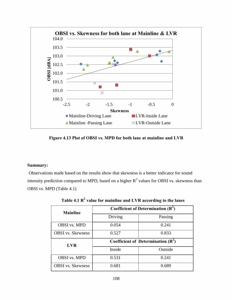
108
Figure 4.13 Plot of OBSI vs. MPD for both lane at mainline and LVR
100.5
101.0
101.5
102.0
102.5
103.0
103.5
104.0
-2.5 -2 -1.5 -1 -0.5 0
OB
SI [d
BA
]
Skewness
OBSI vs. Skewness for both lane at Mainline & LVR
Mainline-Driving Lane LVR-Inside LaneMainline -Passing Lane LVR-Outside Lane
Summary:
Observations made based on the results show that skewness is a better indicator for sound
intensity prediction compared to MPD, based on a higher R2 values for OBSI vs. skewness than
OBSI vs. MPD (Table 4.1)
Table 4.1 R2 value for mainline and LVR according to the lanes
Mainline Coefficient of Determination (R2)
Driving Passing
OBSI vs. MPD 0.054 0.241
OBSI vs. Skewness 0.527 0.833
LVR Coefficient of Determination (R2)
Inside Outside
OBSI vs. MPD 0.531 0.241
OBSI vs. Skewness 0.681 0.689
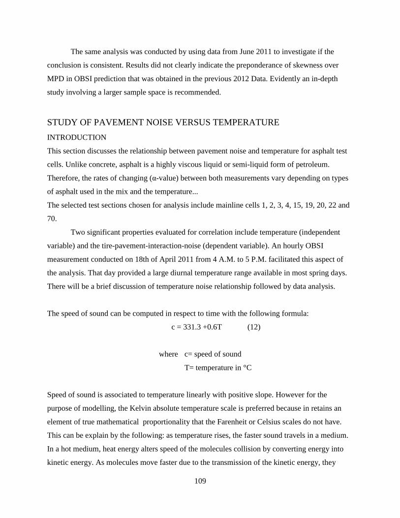
109
The same analysis was conducted by using data from June 2011 to investigate if the
conclusion is consistent. Results did not clearly indicate the preponderance of skewness over
MPD in OBSI prediction that was obtained in the previous 2012 Data. Evidently an in-depth
study involving a larger sample space is recommended.
STUDY OF PAVEMENT NOISE VERSUS TEMPERATURE INTRODUCTION
This section discusses the relationship between pavement noise and temperature for asphalt test
cells. Unlike concrete, asphalt is a highly viscous liquid or semi-liquid form of petroleum.
Therefore, the rates of changing (α-value) between both measurements vary depending on types
of asphalt used in the mix and the temperature...
The selected test sections chosen for analysis include mainline cells 1, 2, 3, 4, 15, 19, 20, 22 and
70.
Two significant properties evaluated for correlation include temperature (independent
variable) and the tire-pavement-interaction-noise (dependent variable). An hourly OBSI
measurement conducted on 18th of April 2011 from 4 A.M. to 5 P.M. facilitated this aspect of
the analysis. That day provided a large diurnal temperature range available in most spring days.
There will be a brief discussion of temperature noise relationship followed by data analysis.
The speed of sound can be computed in respect to time with the following formula:
c = 331.3 +0.6T (12)
where c= speed of sound
T= temperature in °C
Speed of sound is associated to temperature linearly with positive slope. However for the
purpose of modelling, the Kelvin absolute temperature scale is preferred because in retains an
element of true mathematical proportionality that the Farenheit or Celsius scales do not have.
This can be explain by the following: as temperature rises, the faster sound travels in a medium.
In a hot medium, heat energy alters speed of the molecules collision by converting energy into
kinetic energy. As molecules move faster due to the transmission of the kinetic energy, they

110
collide with each other rapidly. Hence, it is safe to say that the hotter the medium, the faster the
sound travels.
Relationship between Density and Temperature:
According to the ideal gas law,
ρ = 𝑃𝑅𝑇
(13)
where ρ = density of medium kg/m3
P = pressure (N/m2)
R = ideal gas constant = 8.314 JK-1mol-1
Temperature is indirectly proportional to density of medium. That is to say, the higher the
temperature is, the denser the medium is. This can be explained by using the kinetic theory as
well. As temperature rises, particles accelerate hence lead to a conversion of kinetic energy to a
mass in a form of new particles. The addition in the mass will leads to denser medium as density
is defined as the mass of the material per unit volume.
Definition of Sound Intensity:
Sound intensity is defined as sound power per unit area. It is a measurement of level differences
in noise.
Sound intensity can be defined mathematically with the formula below:
SI = (14) ρc
where SI = sound int
c =
ρ =
s
d
pe
ens
ed of
ity
s
of
ens
me
ity
dium
ound
As can be observed in the equation, sound intensity can be related in respect to density of
medium. By combining and substituting equation (12) and (13), we get a new relationship of
sound intensity in respect to pressure, gas constant and temperature:
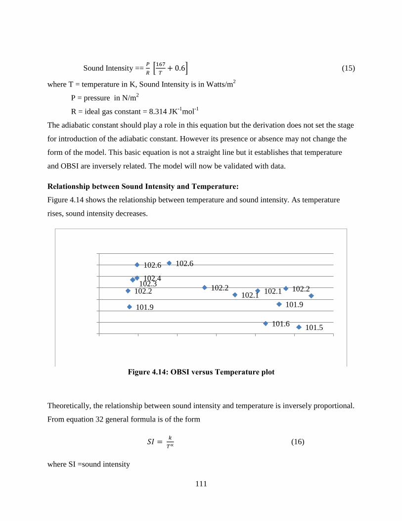
111
Sound Intensity == (15) 𝑃𝑅
�167𝑇
+ 0.6�
where T = temperature in K, Sound Intensity is in Watts/m2
P = pressure in N/m2
R = ideal gas constant = 8.314 JK-1mol-1
The adiabatic constant should play a role in this equation but the derivation does not set the stage
for introduction of the adiabatic constant. However its presence or absence may not change the
form of the model. This basic equation is not a straight line but it establishes that temperature
and OBSI are inversely related. The model will now be validated with data.
Relationship between Sound Intensity and Temperature:
Figure 4.14 shows the relationship between temperature and sound intensity. As temperature
rises, sound intensity decreases.
Figure 4.14: OBSI versus Temperature plot
102.1
101.4101.6101.8
102102.2102.4102.6102.8
272 274 276 278 280 282 284
Soun
d In
tens
ity (d
BA
)
Temperature (Kelvin)
OBSI 12-Hour - Cell 1
Theoretically, the relationship between sound intensity and temperature is inversely proportional.
From equation 32 general formula is of the form
(16) 𝑆𝐼 = 𝑘𝑇∝
where SI =sound intensity
102.2
101.9
102.3 102.4
102.6 102.6
102.2 102.1 102.1
101.6
101.9
102.2
101.5
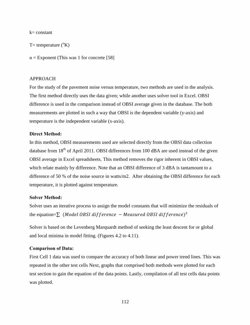
112
k= constant
T= temperature (oK)
α = Exponent (This was 1 for concrete [58]
APPROACH
For the study of the pavement noise versus temperature, two methods are used in the analysis.
The first method directly uses the data given; while another uses solver tool in Excel. OBSI
difference is used in the comparison instead of OBSI average given in the database. The both
measurements are plotted in such a way that OBSI is the dependent variable (y-axis) and
temperature is the independent variable (x-axis).
Direct Method:
In this method, OBSI measurements used are selected directly from the OBSI data collection
database from 18th of April 2011. OBSI differences from 100 dBA are used instead of the given
OBSI average in Excel spreadsheets. This method removes the rigor inherent in OBSI values,
which relate mainly by difference. Note that an OBSI difference of 3 dBA is tantamount to a
difference of 50 % of the noise source in watts/m2. After obtaining the OBSI difference for each
temperature, it is plotted against temperature.
Solver Method:
Solver uses an iterative process to assign the model constants that will minimize the residuals of
the equation=∑ (𝑀𝑜𝑑𝑒𝑙 𝑂𝐵𝑆𝐼 𝑑𝑖𝑓𝑓𝑒𝑟𝑒𝑛𝑐𝑒 −𝑀𝑒𝑎𝑠𝑢𝑟𝑒𝑑 𝑂𝐵𝑆𝐼 𝑑𝑖𝑓𝑓𝑒𝑟𝑒𝑛𝑐𝑒)2
Solver is based on the Levenberg Marquardt method of seeking the least descent for or global
and local minima in model fitting. (Figures 4.2 to 4.11).
Comparison of Data:
First Cell 1 data was used to compare the accuracy of both linear and power trend lines. This was
repeated in the other test cells Next, graphs that comprised both methods were plotted for each
test section to gain the equation of the data points. Lastly, compilation of all test cells data points
was plotted.
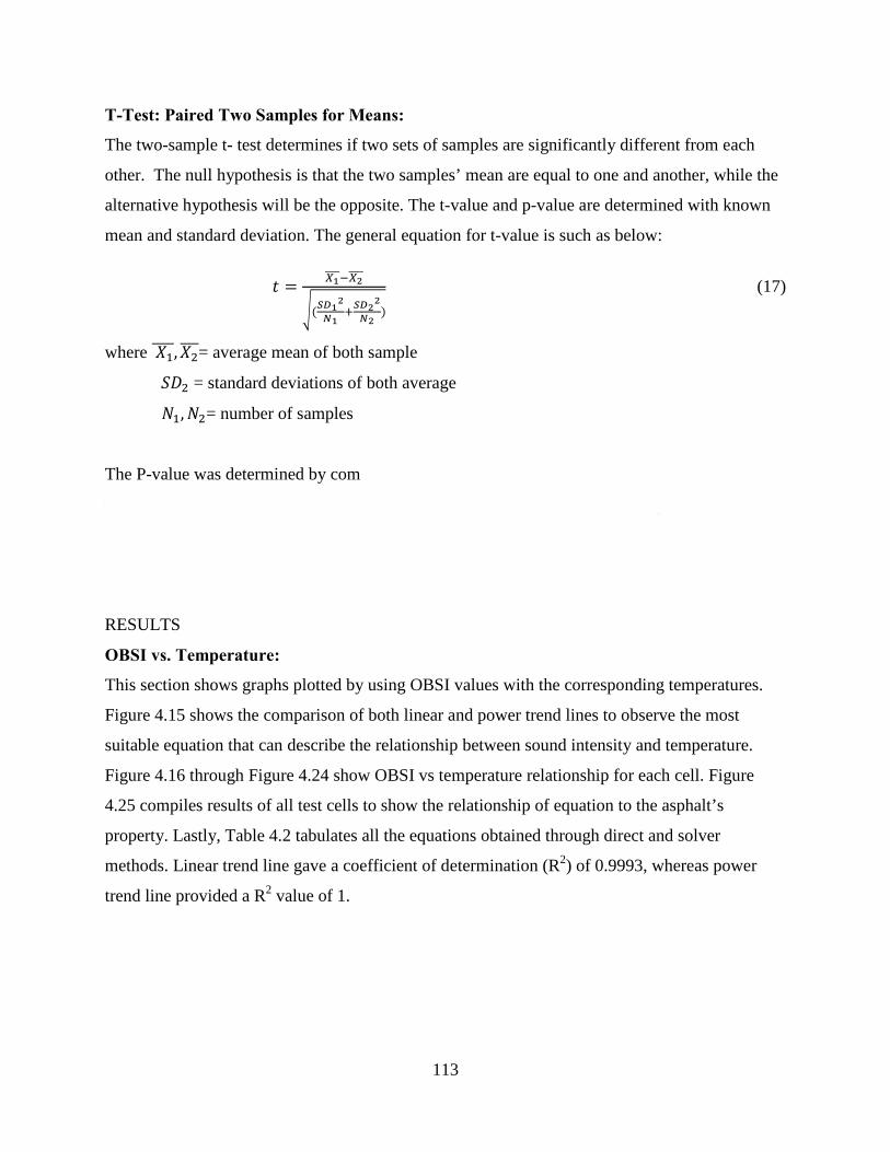
113
T-Test: Paired Two Samples for Means:
The two-sample t- test determines if two sets of samples are significantly different from each
other. The null hypothesis is that the two samples’ mean are equal to one and another, while the
alternative hypothesis will be the opposite. The t-value and p-value are determined with known
mean and standard deviation. The general equation for t-value is such as below:
𝑡 = 𝑋1����−𝑋2����
�(𝑆𝐷12
𝑁1
(17) +𝑆𝐷2
2
𝑁2)
where
𝑆𝐷2
= average mean of both sample
1
The P-va
𝑁
lue
,𝑁
=
2
standard deviations of both average
= number of samples
was determined by comparing the calculated t-value with a standard table of t-
values to determine whether the t-statistic reaches the threshold of statistical significance. The
null hypothesis will be rejected when P-value is lesser than the significant level (i.e. 0.05 for a
95% confidence level) and vice versa.
𝑋1����,𝑋2���
RESULTS
OBSI vs. Temperature:
This section shows graphs plotted by using OBSI values with the corresponding temperatures.
Figure 4.15 shows the comparison of both linear and power trend lines to observe the most
suitable equation that can describe the relationship between sound intensity and temperature.
Figure 4.16 through Figure 4.24 show OBSI vs temperature relationship for each cell. Figure
4.25 compiles results of all test cells to show the relationship of equation to the asphalt’s
property. Lastly, Table 4.2 tabulates all the equations obtained through direct and solver
methods. Linear trend line gave a coefficient of determination (R2) of 0.9993, whereas power
trend line provided a R2 value of 1.
114
1.5
1.7
1.9
2.1
2.3
2.5
272 274 276 278 280 282 284OB
SI D
iffer
ence
[dB
A]
Temperature [Kelvin]
OBSI vs. Temperature- Cell 1 Comparison of trendline
Linear (OBSI vs. Temperature- Cell 1)Power (OBSI vs. Temperature- Cell 1)
Figure 4.15: Comparison of Linear Trend line and Power Trend line for cell 1
Red data points are the data obtained from using solver method, whereas blue data points are the
data gotten from using direct method.
Figure 4.16 Plot of OBSI Difference versus Temperature for cell 1
y = 1E+17x-6.865
y = 2E+15x-6.092
0.00.51.01.52.02.53.0
272 274 276 278 280 282 284
OB
SI D
iffer
ence
[dB
A]
Temperature [Kelvin]
OBSI Difference vs. Temperature -Cell 1
OBSI-12-hour Cell 1 OBSI-Solver Cell 1Power (OBSI-12-hour Cell 1) Power (OBSI-Solver Cell 1)
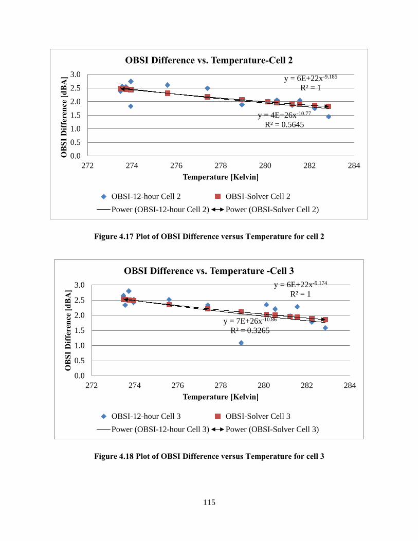
115
Figure 4.17 Plot of OBSI Difference versus Temperature for cell 2
y = 4E+26x-10.77 R² = 0.5645
y = 6E+22x-9.185 R² = 1
0.0
0.5
1.0
1.5
2.0
2.5
3.0
272 274 276 278 280 282 284
OB
SI D
iffer
ence
[dB
A]
Temperature [Kelvin]
OBSI Difference vs. Temperature-Cell 2
OBSI-12-hour Cell 2 OBSI-Solver Cell 2Power (OBSI-12-hour Cell 2) Power (OBSI-Solver Cell 2)
Figure 4.18 Plot of OBSI Difference versus Temperature for cell 3
y = 7E+26x-10.86 R² = 0.3265
y = 6E+22x-9.174 R² = 1
0.0
0.5
1.0
1.5
2.0
2.5
3.0
272 274 276 278 280 282 284
OB
SI D
iffer
ence
[dB
A]
Temperature [Kelvin]
OBSI Difference vs. Temperature -Cell 3
OBSI-12-hour Cell 3 OBSI-Solver Cell 3Power (OBSI-12-hour Cell 3) Power (OBSI-Solver Cell 3)
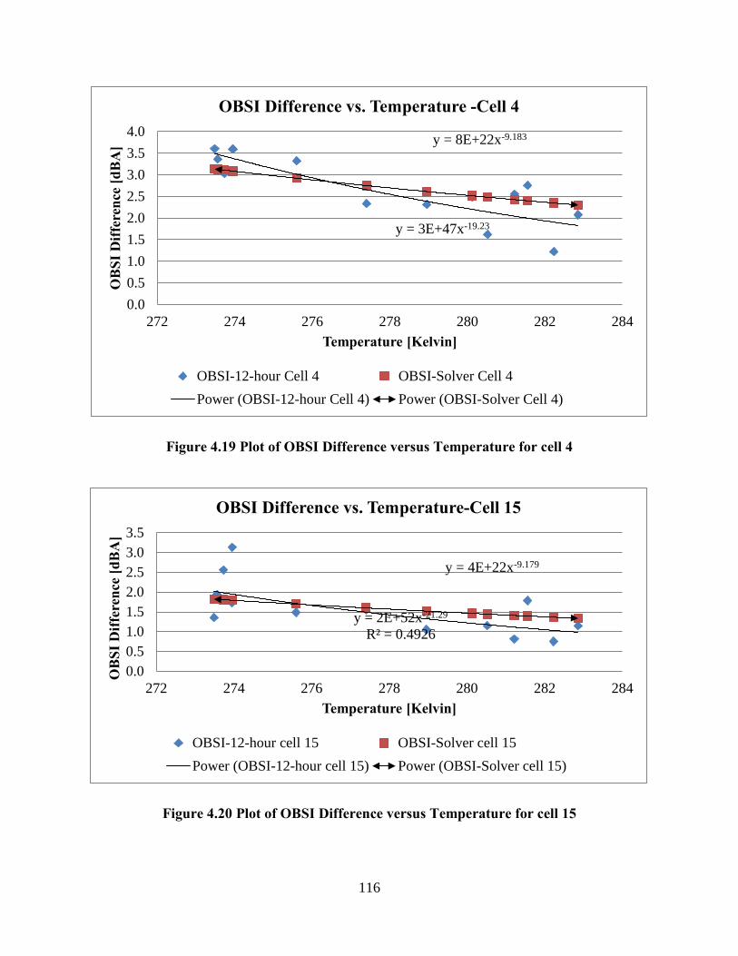
116
Figure 4.19 Plot of OBSI Difference versus Temperature for cell 4
y = 3E+47x-19.23
y = 8E+22x-9.183
0.00.51.01.52.02.53.03.54.0
272 274 276 278 280 282 284
OB
SI D
iffer
ence
[dB
A]
Temperature [Kelvin]
OBSI Difference vs. Temperature -Cell 4
OBSI-12-hour Cell 4 OBSI-Solver Cell 4Power (OBSI-12-hour Cell 4) Power (OBSI-Solver Cell 4)
Figure 4.20 Plot of OBSI Difference versus Temperature for cell 15
y = 2E+52x-21.29 R² = 0.4926
y = 4E+22x-9.179
0.00.51.01.52.02.53.03.5
272 274 276 278 280 282 284
OB
SI D
iffer
ence
[dB
A]
Temperature [Kelvin]
OBSI Difference vs. Temperature-Cell 15
OBSI-12-hour cell 15 OBSI-Solver cell 15Power (OBSI-12-hour cell 15) Power (OBSI-Solver cell 15)
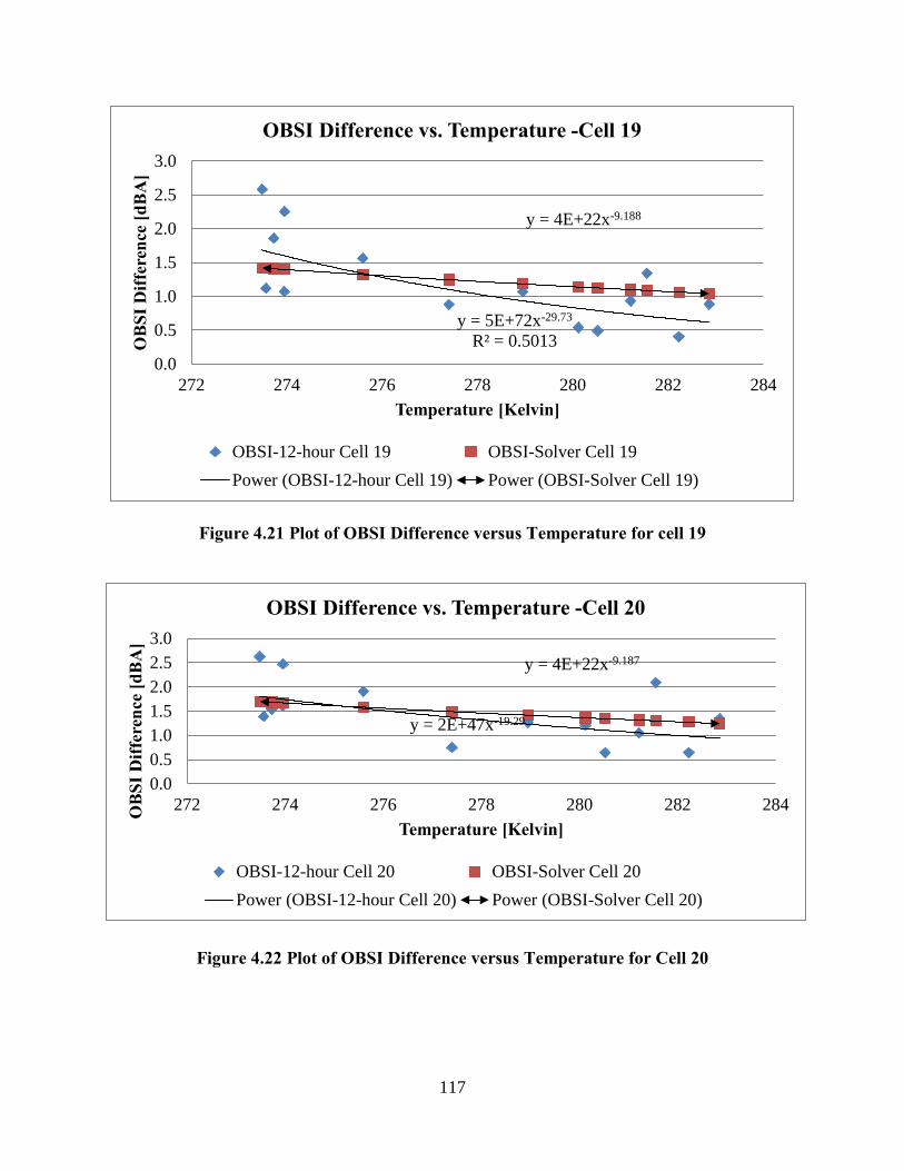
117
Figure 4.21 Plot of OBSI Difference versus Temperature for cell 19
y = 5E+72x-29.73 R² = 0.5013
y = 4E+22x-9.188
0.0
0.5
1.0
1.5
2.0
2.5
3.0
272 274 276 278 280 282 284
OB
SI D
iffer
ence
[dB
A]
Temperature [Kelvin]
OBSI Difference vs. Temperature -Cell 19
OBSI-12-hour Cell 19 OBSI-Solver Cell 19Power (OBSI-12-hour Cell 19) Power (OBSI-Solver Cell 19)
Figure 4.22 Plot of OBSI Difference versus Temperature for Cell 20
y = 2E+47x-19.29
y = 4E+22x-9.187
0.00.51.01.52.02.53.0
272 274 276 278 280 282 284OB
SI D
iffer
ence
[dB
A]
Temperature [Kelvin]
OBSI Difference vs. Temperature -Cell 20
OBSI-12-hour Cell 20 OBSI-Solver Cell 20Power (OBSI-12-hour Cell 20) Power (OBSI-Solver Cell 20)
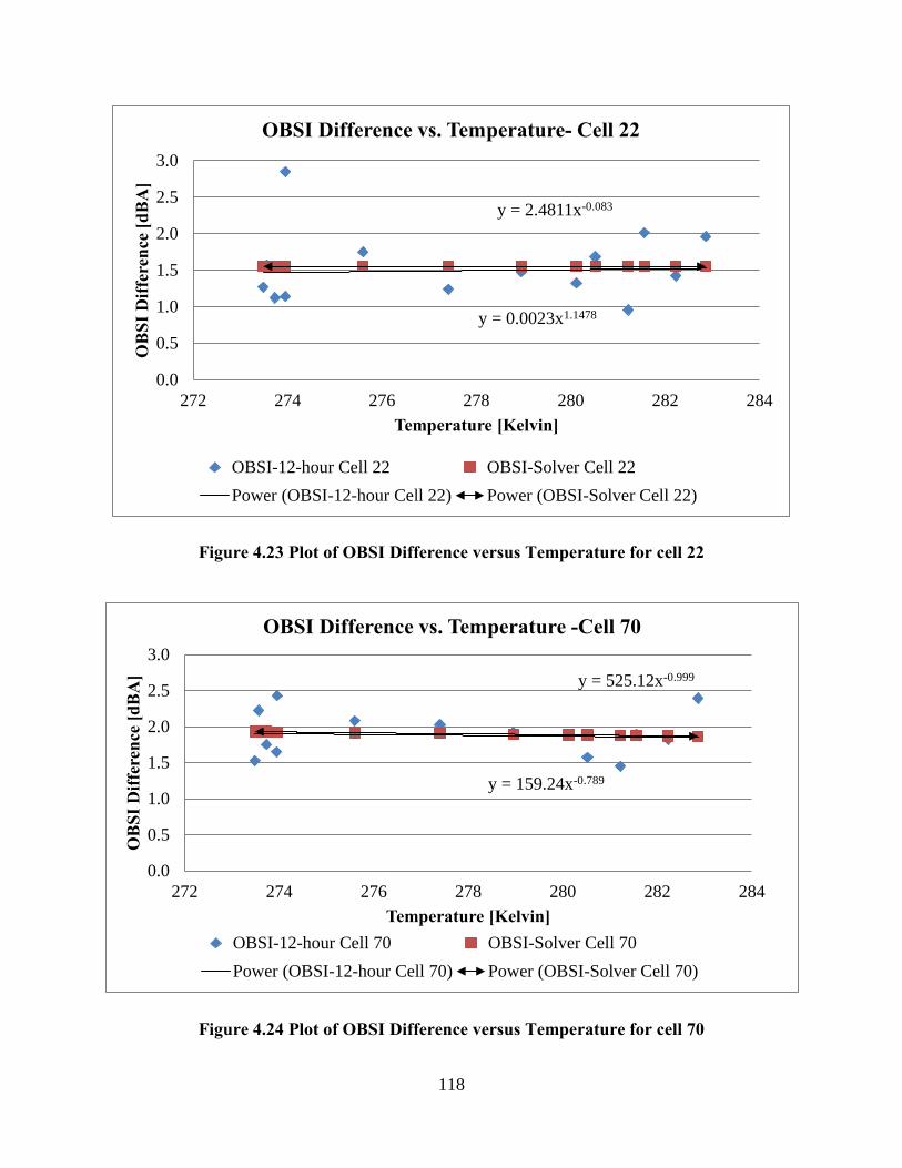
118
Figure 4.23 Plot of OBSI Difference versus Temperature for cell 22
Figure 4.24 Plot of OBSI Difference versus Temperature for cell 70
y = 0.0023x1.1478
y = 2.4811x-0.083
0.0
0.5
1.0
1.5
2.0
2.5
3.0
272 274 276 278 280 282 284
OB
SI D
iffer
ence
[dB
A]
Temperature [Kelvin]
OBSI Difference vs. Temperature- Cell 22
OBSI-12-hour Cell 22 OBSI-Solver Cell 22Power (OBSI-12-hour Cell 22) Power (OBSI-Solver Cell 22)
y = 159.24x-0.789
y = 525.12x-0.999
0.0
0.5
1.0
1.5
2.0
2.5
3.0
272 274 276 278 280 282 284
OB
SI D
iffer
ence
[dB
A]
Temperature [Kelvin]
OBSI Difference vs. Temperature -Cell 70
OBSI-12-hour Cell 70 OBSI-Solver Cell 70Power (OBSI-12-hour Cell 70) Power (OBSI-Solver Cell 70)
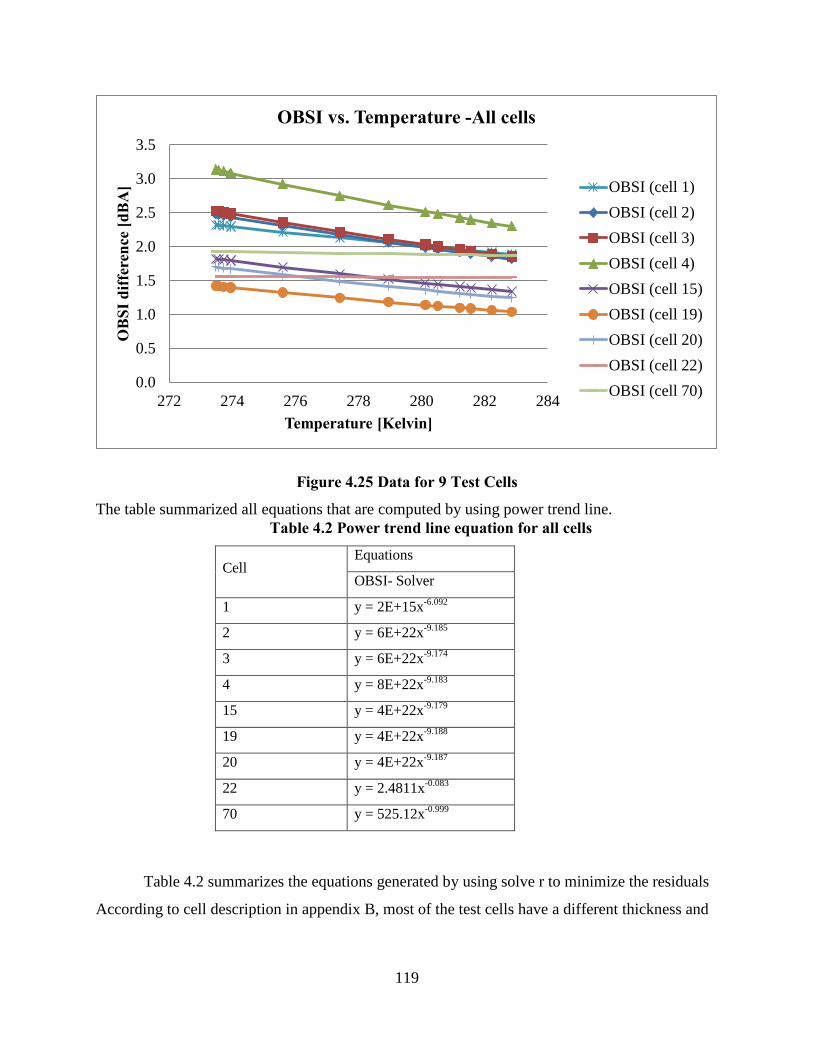
119
Figure 4.25 Data for 9 Test Cells
0.0
0.5
1.0
1.5
2.0
2.5
3.0
3.5
272 274 276 278 280 282 284
OB
SI d
iffer
ence
[dB
A]
Temperature [Kelvin]
OBSI vs. Temperature -All cells
OBSI (cell 1)OBSI (cell 2)OBSI (cell 3)OBSI (cell 4)OBSI (cell 15)OBSI (cell 19)OBSI (cell 20)OBSI (cell 22)OBSI (cell 70)
The table summarized all equations that are computed by using power trend line. Table 4.2 Power trend line equation for all cells
Cell Equations
OBSI- Solver
1 y = 2E+15x-6.092
2 y = 6E+22x-9.185
3 y = 6E+22x-9.174
4 y = 8E+22x-9.183
15 y = 4E+22x-9.179
19 y = 4E+22x-9.188
20 y = 4E+22x-9.187
22 y = 2.4811x-0.083
70 y = 525.12x-0.999
Table 4.2 summarizes the equations generated by using solve r to minimize the residuals
According to cell description in appendix B, most of the test cells have a different thickness and
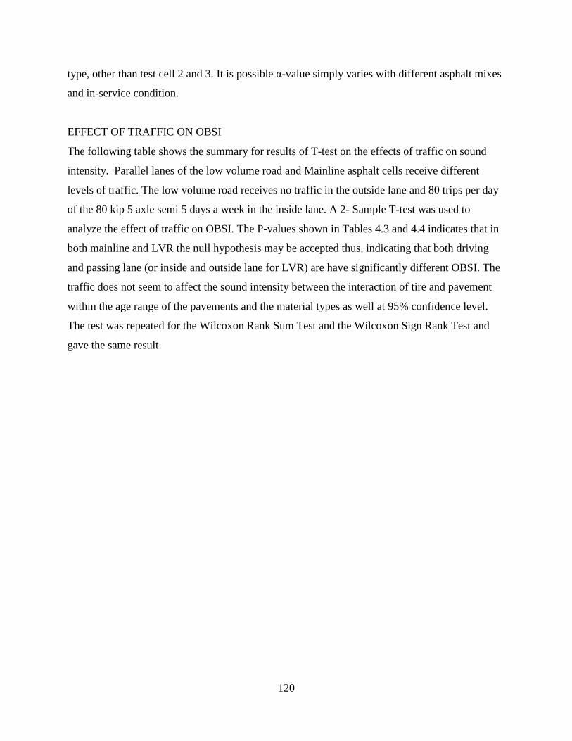
120
type, other than test cell 2 and 3. It is possible α-value simply varies with different asphalt mixes
and in-service condition.
EFFECT OF TRAFFIC ON OBSI
The following table shows the summary for results of T-test on the effects of traffic on sound
intensity. Parallel lanes of the low volume road and Mainline asphalt cells receive different
levels of traffic. The low volume road receives no traffic in the outside lane and 80 trips per day
of the 80 kip 5 axle semi 5 days a week in the inside lane. A 2- Sample T-test was used to
analyze the effect of traffic on OBSI. The P-values shown in Tables 4.3 and 4.4 indicates that in
both mainline and LVR the null hypothesis may be accepted thus, indicating that both driving
and passing lane (or inside and outside lane for LVR) are have significantly different OBSI. The
traffic does not seem to affect the sound intensity between the interaction of tire and pavement
within the age range of the pavements and the material types as well at 95% confidence level.
The test was repeated for the Wilcoxon Rank Sum Test and the Wilcoxon Sign Rank Test and
gave the same result.
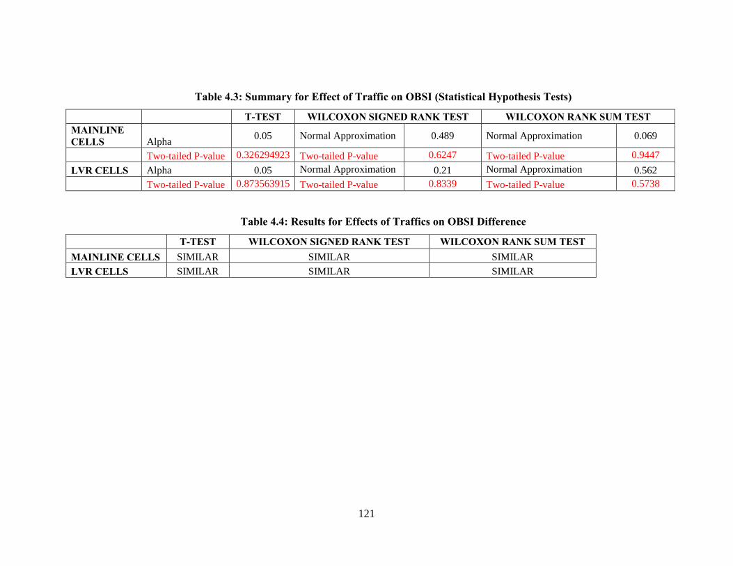
121
Table 4.3: Summary for Effect of Traffic on OBSI (Statistical Hypothesis Tests)
T-TEST WILCOXON SIGNED RANK TEST WILCOXON RANK SUM TEST MAINLINE CELLS Alpha 0.05 Normal Approximation 0.489 Normal Approximation 0.069
Two-tailed P-value 0.326294923 Two-tailed P-value 0.6247 Two-tailed P-value 0.9447 LVR CELLS Alpha 0.05 Normal Approximation 0.21 Normal Approximation 0.562 Two-tailed P-value 0.873563915 Two-tailed P-value 0.8339 Two-tailed P-value 0.5738
Table 4.4: Results for Effects of Traffics on OBSI Difference
T-TEST WILCOXON SIGNED RANK TEST WILCOXON RANK SUM TEST MAINLINE CELLS SIMILAR SIMILAR SIMILAR LVR CELLS SIMILAR SIMILAR SIMILAR
122
FRICTIONAL PROPERTIES ON ASPHALT PAVEMENT SURFACES INTRODUCTION
This section examines the differences between friction number of smooth and ribbed tires to
possibly identify hysteresis phenomenon and to determine how frictional resistance changes in
asphalt pavements. Fragmentation of Friction al forces into hysteresis and adhesion forces is
expected to characterize frictional properties better.
Cells 1 through 4 were used to observe the behavior of frictional properties between
smooth tires and ribbed tires. Cell 3, 4, 19, and 22 were used to compare the coefficient of
friction at the speed of 40km/hr.; and observation is made based on the type of asphalt pavement.
The type of pavements for all these cells are: cell 1 has original hot-mixed asphalt; cell 2, 3 and 4
have stabilized full depth reclamation asphalt; cell 19 has recycled unbound base, warm mix
asphalt; and cell 22 has low temperature cracking, fractionated reclamation asphalt. Data were
retrieved from year 2007 to year 2012.
The purpose of the study for behavior of frictional properties between two types of tires
is to identify the occurrences of hysteresis phenomenon on asphalt pavements; while the
comparison of the coefficient of friction at the speed of 40km/hr. is to observe the differences in
pattern of the frictional properties based on the type of asphalt pavements.
Friction is the force resisting the relative motion of surfaces. It moves in the opposite
direction of the motion. The measurement of friction varies based on the coefficient of friction
depending on the surface, which will be discussed in next Section.
Frictional properties play an important role in the analysis of pavement performance. The
two main component of friction in tire-pavement interaction comprises of adhesion and
hysteresis. Adhesion force, Fa is produced by the actual contact area between tire and pavement
surface. Theoretically, energy that resists breakage of surface-to-surface contact forces in the
direction of motion is friction and plane of contact is the frictional resistance. This energy is the
work done by the adhesion force. On the other hand, hysteresis exists when there is deformation
of rubber tire due to pavement surface asperities [58]. Hysteresis occurs when the rubber is
alternately compressed and relaxed when travelling in an uneven pavement surface [58].
Hysteresis can be explained in such a manner: the “relaxing” process did not happen right after
“compression” process because of a phenomenon called suction. Suction forces the tire to adhere
to the pavement surface due to the differences in external and internal pressures. It depends on
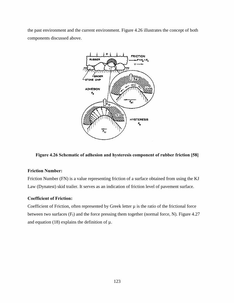
123
the past environment and the current environment. Figure 4.26 illustrates the concept of both
components discussed above.
Figure 4.26 Schematic of adhesion and hysteresis component of rubber friction [58]
Friction Number:
Friction Number (FN) is a value representing friction of a surface obtained from using the KJ
Law (Dynatest) skid trailer. It serves as an indication of friction level of pavement surface.
Coefficient of Friction:
Coefficient of Friction, often represented by Greek letter µ is the ratio of the frictional force
between two surfaces (Ff) and the force pressing them together (normal force, N). Figure 4.27
and equation (18) explains the definition of µ.
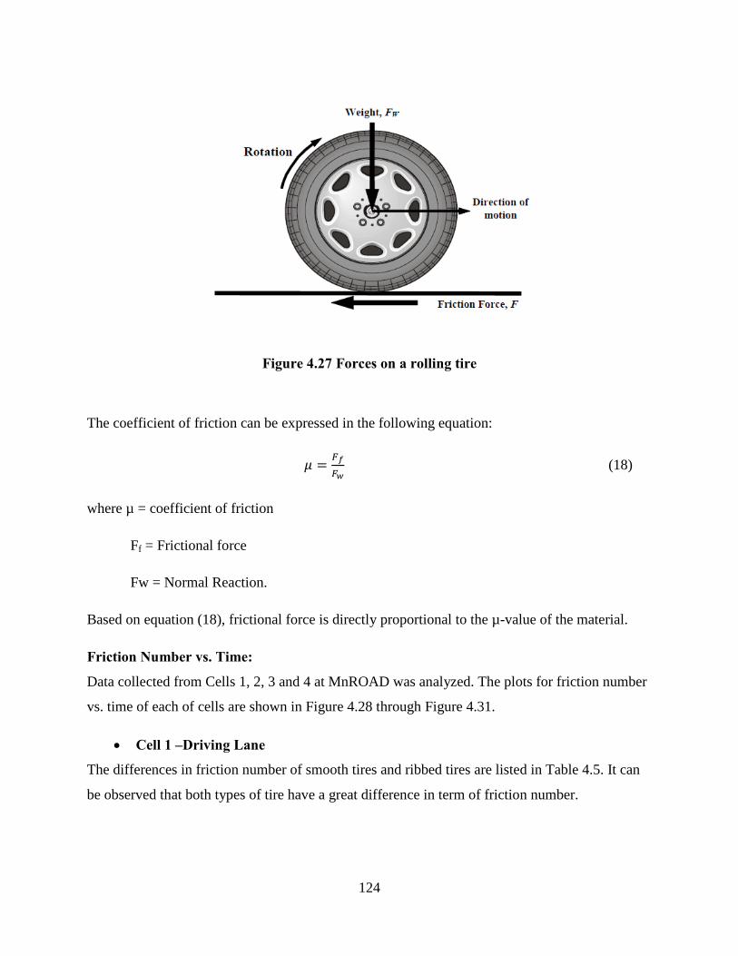
124
Figure 4.27 Forces on a rolling tire
The coefficient of friction can be expressed in the following equation:
𝜇 = 𝐹𝑓𝐹𝑤
(18)
where µ = coefficient of friction
Ff = Frictional force
Fw = Normal Reaction.
Based on equation (18), frictional force is directly proportional to the µ-value of the material.
Friction Number vs. Time:
Data collected from Cells 1, 2, 3 and 4 at MnROAD was analyzed. The plots for friction number
vs. time of each of cells are shown in Figure 4.28 through Figure 4.31.
• Cell 1 –Driving Lane
The differences in friction number of smooth tires and ribbed tires are listed in Table 4.5. It can
be observed that both types of tire have a great difference in term of friction number.
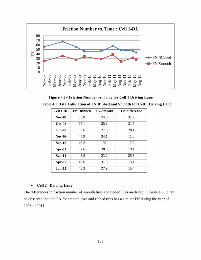
125
Figure 4.28 Friction Number vs. Time for Cell 1 Driving Lane
01020304050607080
Nov
-07
Feb-
08M
ay-0
8A
ug-0
8N
ov-0
8Fe
b-09
May
-09
Aug
-09
Nov
-09
Feb-
10M
ay-1
0A
ug-1
0N
ov-1
0Fe
b-11
May
-11
Aug
-11
Nov
-11
Feb-
12M
ay-1
2A
ug-1
2
FN
Friction Number vs. Time : Cell 1-DL
FN /RibbedFN/Smooth
Table 4.5 Data Tabulation of FN Ribbed and Smooth for Cell 1 Driving Lane
Cell 1 DL FN /Ribbed FN/Smooth FN difference
Nov-07 55.8 24.6 31.2
Oct-08 67.1 35.6 31.5
Jun-09 55.6 27.5 28.1
Nov-09 45.9 34.1 11.8
Sep-10 46.2 29 17.2
Apr-11 57.6 38.5 19.1
Sep-11 48.5 23.2 25.3
Apr-12 46.6 31.5 15.1
Jun-12 43.3 27.9 15.4
• Cell 2 –Driving Lane
The differences in friction number of smooth tires and ribbed tires are listed in Table 4.6. It can
be observed that the FN for smooth tires and ribbed tires has a similar FN during the year of
2008 to 2011.
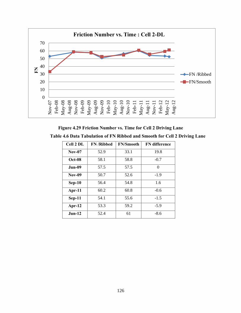
126
Figure 4.29 Friction Number vs. Time for Cell 2 Driving Lane
010203040506070
Nov
-07
Feb-
08M
ay-0
8A
ug-0
8N
ov-0
8Fe
b-09
May
-09
Aug
-09
Nov
-09
Feb-
10M
ay-1
0A
ug-1
0N
ov-1
0Fe
b-11
May
-11
Aug
-11
Nov
-11
Feb-
12M
ay-1
2A
ug-1
2
FN
Friction Number vs. Time : Cell 2-DL
FN /RibbedFN/Smooth
Table 4.6 Data Tabulation of FN Ribbed and Smooth for Cell 2 Driving Lane
Cell 2 DL FN /Ribbed FN/Smooth FN difference
Nov-07 52.9 33.1 19.8
Oct-08 58.1 58.8 -0.7
Jun-09 57.5 57.5 0
Nov-09 50.7 52.6 -1.9
Sep-10 56.4 54.8 1.6
Apr-11 60.2 60.8 -0.6
Sep-11 54.1 55.6 -1.5
Apr-12 53.3 59.2 -5.9
Jun-12 52.4 61 -8.6
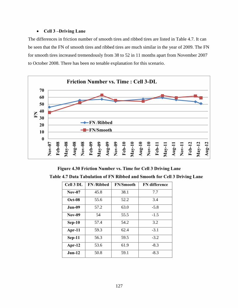
127
• Cell 3 –Driving Lane
The differences in friction number of smooth tires and ribbed tires are listed in Table 4.7. It can
be seen that the FN of smooth tires and ribbed tires are much similar in the year of 2009. The FN
for smooth tires increased tremendously from 38 to 52 in 11 months apart from November 2007
to October 2008. There has been no tenable explanation for this scenario.
Figure 4.30 Friction Number vs. Time for Cell 3 Driving Lane
010203040506070
Nov
-07
Feb-
08
May
-08
Aug
-08
Nov
-08
Feb-
09
May
-09
Aug
-09
Nov
-09
Feb-
10
May
-10
Aug
-10
Nov
-10
Feb-
11
May
-11
Aug
-11
Nov
-11
Feb-
12
May
-12
Aug
-12
FN
Friction Number vs. Time : Cell 3-DL
FN /RibbedFN/Smooth
Table 4.7 Data Tabulation of FN Ribbed and Smooth for Cell 3 Driving Lane
Cell 3 DL FN /Ribbed FN/Smooth FN difference
Nov-07 45.8 38.1 7.7
Oct-08 55.6 52.2 3.4
Jun-09 57.2 63.0 -5.8
Nov-09 54 55.5 -1.5
Sep-10 57.4 54.2 3.2
Apr-11 59.3 62.4 -3.1
Sep-11 56.3 59.5 -3.2
Apr-12 53.6 61.9 -8.3
Jun-12 50.8 59.1 -8.3
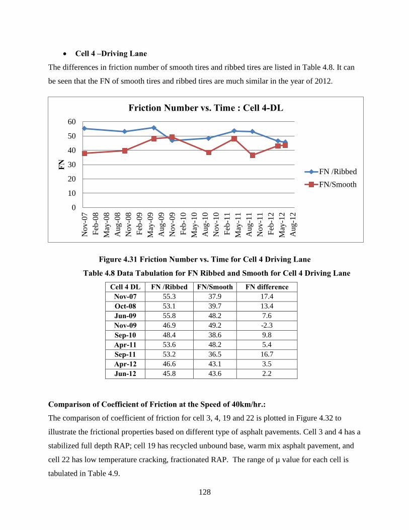
128
• Cell 4 –Driving Lane
The differences in friction number of smooth tires and ribbed tires are listed in Table 4.8. It can
be seen that the FN of smooth tires and ribbed tires are much similar in the year of 2012.
Figure 4.31 Friction Number vs. Time for Cell 4 Driving Lane
0
10
20
30
40
50
60
Nov
-07
Feb-
08M
ay-0
8A
ug-0
8N
ov-0
8Fe
b-09
May
-09
Aug
-09
Nov
-09
Feb-
10M
ay-1
0A
ug-1
0N
ov-1
0Fe
b-11
May
-11
Aug
-11
Nov
-11
Feb-
12M
ay-1
2A
ug-1
2
FN
Friction Number vs. Time : Cell 4-DL
FN /RibbedFN/Smooth
Table 4.8 Data Tabulation for FN Ribbed and Smooth for Cell 4 Driving Lane
Cell 4 DL FN /Ribbed FN/Smooth FN difference Nov-07 55.3 37.9 17.4 Oct-08 53.1 39.7 13.4 Jun-09 55.8 48.2 7.6 Nov-09 46.9 49.2 -2.3 Sep-10 48.4 38.6 9.8 Apr-11 53.6 48.2 5.4 Sep-11 53.2 36.5 16.7 Apr-12 46.6 43.1 3.5 Jun-12 45.8 43.6 2.2
Comparison of Coefficient of Friction at the Speed of 40km/hr.:
The comparison of coefficient of friction for cell 3, 4, 19 and 22 is plotted in Figure 4.32 to
illustrate the frictional properties based on different type of asphalt pavements. Cell 3 and 4 has a
stabilized full depth RAP; cell 19 has recycled unbound base, warm mix asphalt pavement, and
cell 22 has low temperature cracking, fractionated RAP. The range of µ value for each cell is
tabulated in Table 4.9.
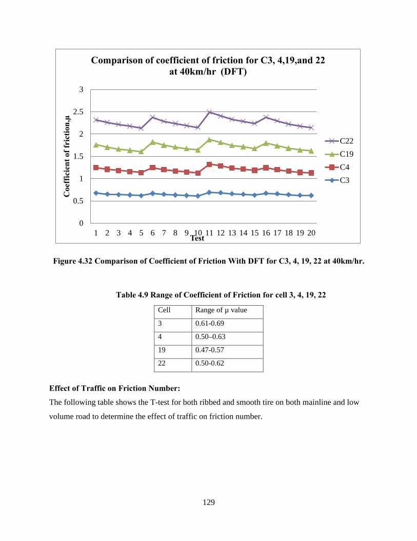
129
Figure 4.32 Comparison of Coefficient of Friction With DFT for C3, 4, 19, 22 at 40km/hr.
0
0.5
1
1.5
2
2.5
3
1 2 3 4 5 6 7 8 9 10 11 12 13 14 15 16 17 18 19 20
Coe
ffic
ient
of f
rict
ion,
µ
Test
Comparison of coefficient of friction for C3, 4,19,and 22 at 40km/hr (DFT)
C22C19C4C3
Table 4.9 Range of Coefficient of Friction for cell 3, 4, 19, 22
Cell Range of µ value
3 0.61-0.69
4 0.50–0.63
19 0.47-0.57
22 0.50-0.62
Effect of Traffic on Friction Number:
The following table shows the T-test for both ribbed and smooth tire on both mainline and low
volume road to determine the effect of traffic on friction number.
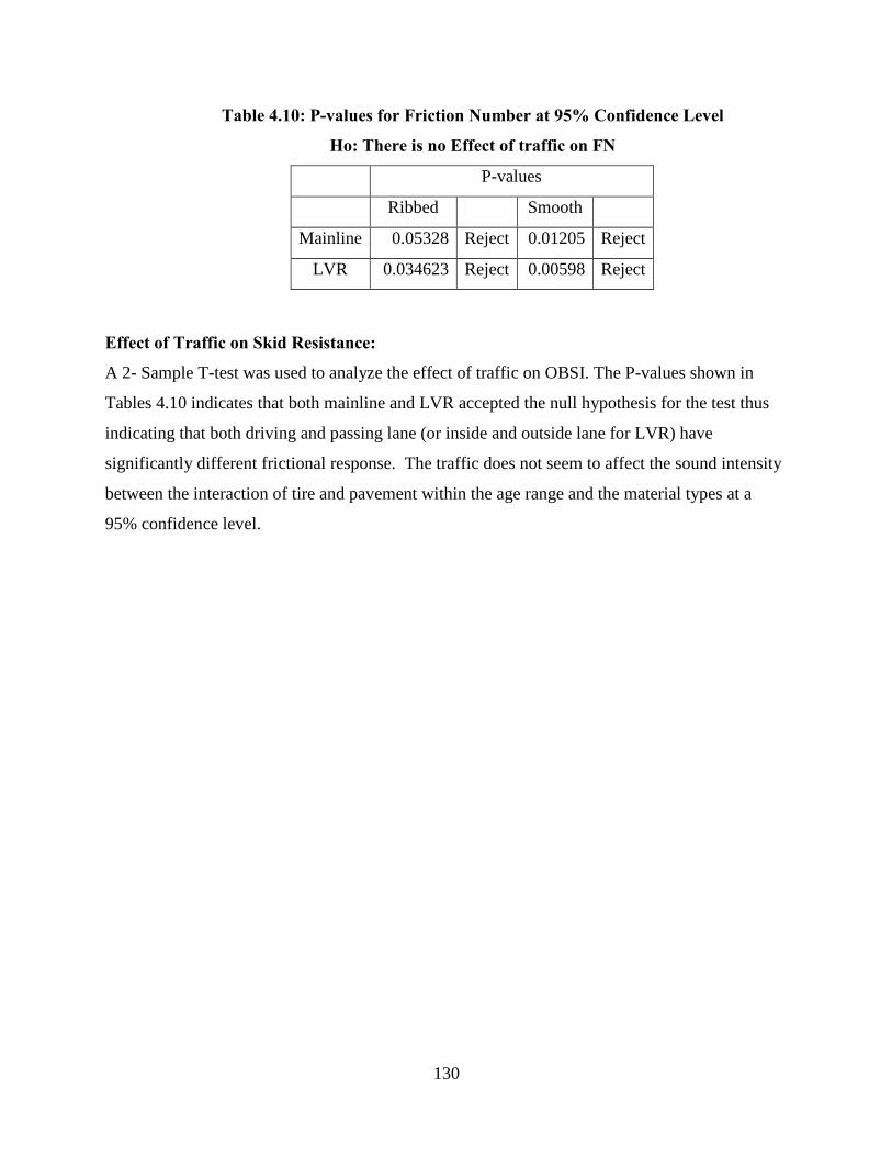
130
Table 4.10: P-values for Friction Number at 95% Confidence Level
Ho: There is no Effect of traffic on FN
P-values
Ribbed Smooth
Mainline 0.05328 Reject 0.01205 Reject
LVR 0.034623 Reject 0.00598 Reject
Effect of Traffic on Skid Resistance:
A 2- Sample T-test was used to analyze the effect of traffic on OBSI. The P-values shown in
Tables 4.10 indicates that both mainline and LVR accepted the null hypothesis for the test thus
indicating that both driving and passing lane (or inside and outside lane for LVR) have
significantly different frictional response. The traffic does not seem to affect the sound intensity
between the interaction of tire and pavement within the age range and the material types at a
95% confidence level.
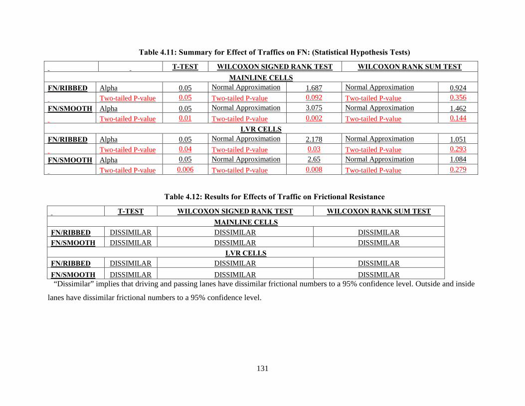
131
Table 4.11: Summary for Effect of Traffics on FN: (Statistical Hypothesis Tests)
T-TEST WILCOXON SIGNED RANK TEST WILCOXON RANK SUM TEST MAINLINE CELLS
FN/RIBBED Alpha 0.05 Normal Approximation 1.687 Normal Approximation 0.924 Two-tailed P-value 0.05 Two-tailed P-value 0.092 Two-tailed P-value 0.356 FN/SMOOTH Alpha 0.05 Normal Approximation 3.075 Normal Approximation 1.462 Two-tailed P-value 0.01 Two-tailed P-value 0.002 Two-tailed P-value 0.144
LVR CELLS FN/RIBBED Alpha 0.05 Normal Approximation 2.178 Normal Approximation 1.051 Two-tailed P-value 0.04 Two-tailed P-value 0.03 Two-tailed P-value 0.293 FN/SMOOTH Alpha 0.05 Normal Approximation 2.65 Normal Approximation 1.084 Two-tailed P-value 0.006 Two-tailed P-value 0.008 Two-tailed P-value 0.279
Table 4.12: Results for Effects of Traffic on Frictional Resistance
T-TEST WILCOXON SIGNED RANK TEST WILCOXON RANK SUM TEST MAINLINE CELLS
FN/RIBBED DISSIMILAR DISSIMILAR DISSIMILAR FN/SMOOTH DISSIMILAR DISSIMILAR DISSIMILAR
LVR CELLS FN/RIBBED DISSIMILAR DISSIMILAR DISSIMILAR FN/SMOOTH DISSIMILAR DISSIMILAR DISSIMILAR
“Dissimilar” implies that driving and passing lanes have dissimilar frictional numbers to a 95% confidence level. Outside and inside
lanes have dissimilar frictional numbers to a 95% confidence level.
132
Friction Number vs. Time:
The difference of FN between both types of tires in cell 1 is significantly large. This indicates
that from 2007 to 2012 hysteresis effect may be infinitesimal. In cell 2, a huge gap of FN
between smooth and ribbed tires occurred only from November 2007 to September 2008. The
main reason behind this occurrence is that cell was reconstructed on October 2008, therefore the
differences of FN for both tires from October 2008 to September 2011 falls in the range of 0 to
1.5. Hysteresis as discussed earlier on the Chapter is a system where it depends on the past and
current environment, so that is the reason why the difference of the newly reconstructed cell on
October 2008 has a low difference in FN. The differences of FN between both tires increases
after August 2011, indicates that hysteresis occurs.
Cell 3 shows a different pattern as compare to cell 2 even though cell 3 was reconstructed
at the same time as cell 2 and has similar type of asphalt pavement. The differences of FN
fluctuate throughout year 2007 to year 2012. The largest difference of FN occurs in year 2012,
which has a difference of 8.3 between ribbed and smooth tire friction.
Cell 4 is observed to have a large difference in friction number from November 2007 to October
2009 and fluctuate into a smaller gap in difference at the end of year 2009. However, the
differences in friction number increases from September 2010 to March 2012. The differences
then decreases gradually from April 2012 to June 2012.
Comparison for Coefficient of Friction of Cells at 40km/hr:
The comparison of coefficient of friction for cell 3, 4, 19 and 22 can be found in Figure 4.32 in
the results section. The trends in all four cells are similar to each other. However, it is obvious
that the range of the µ value for cell three is much higher than the other cells. This is due to the
type of asphalt pavements (Appendix 4.A, Figure 4.A.2). Even though cell 3 and 4 are stabilized
full depth reclamation asphalt, cell 3 has an ultra-thin-bonded wearing course (UTWBC) on the
top layer of the pavement. UTWBC is a material does not seem to experience aggregate rapid
polishing or aggregate loss, therefore it provides excellent adhesion properties and friction on
pavement. It can be proven with the differences in range of µ value between cell 3 and 4. Other
than that, cell 3 has the higher range of coefficient of friction among the four cells, which is in
the range of 0.61- 0.69. Cell 4 as mentioned above has a second highest friction value, which
falls in the range of 0.50 – 0.63.
133
Cell 19 has recycled unbounded base and warm mix asphalt pavement has a µ range of
0.47 to 0.57. Cell 22 has a similar friction factor with cell 4. It may be due to the type of
pavement surface of cell 22. Its range of µ value falls in between 0.50 to 0.62.
Two-Sample T-test was used to analyze the effect of traffic on friction number. The P-values
shown in Table 4.3.6 in the results section indicates that both mainline and LVR rejected the null
hypothesis for both ribbed and smooth tires. This means that both driving and passing lane (or
inside and outside lane for LVR) is significantly different. It can be deduced that the traffic does
affect the friction number based on the preliminary study on effect of traffic on friction number.
The heavy traffic on driving lane may cause an increment in deterioration of friction in
comparison to passing lane.
Preliminary Half-life Friction Extrapolations:
This section depicts the relationship between the rate of friction degradation and friction number.
It is hypothesized that the friction degradation will follow a pattern of decay, similarly to the
half-life equation. A preliminary analysis was conducted on test cell 2, 3, 4 and 27. Test cell 2, 3
and 4 are stabilized full depth reclamation pavement first constructed on September 28, 1992.
Both cell 2 and 3 were reconstructed with added ultra-thin bonded wearing course in October
2008. As for test cell 4, it was covered with dense graded SuperPave during the reconstruction in
October 2008. Test cell 27 was built on August 15, 1992 and the double chip seal was added on
August 15, 1999. The analysis was done based on the decay equation:
𝐹𝑁𝑡 = 𝐹𝑁𝑜𝑒−𝜆𝑡 (19)
Where FNt = friction number at year t
FNo = friction number immediately after construction (at the zeroth year)
λ = decay constant
t= time (Yrs) 𝐹𝑁𝑡 (20) ln𝐹𝑁𝑜
= −𝜆𝑡
The slope of versus time graph is the decay constant, λ-value based on equation 38. The
λ-value is used to find the half-life for each cell using the following equation:
ln 𝐹𝑁𝑡𝐹𝑁𝑜
𝑡1/2 = ln 2𝜆
(21)
The table below shows the results of half-life analysis for the test cells by the described method.
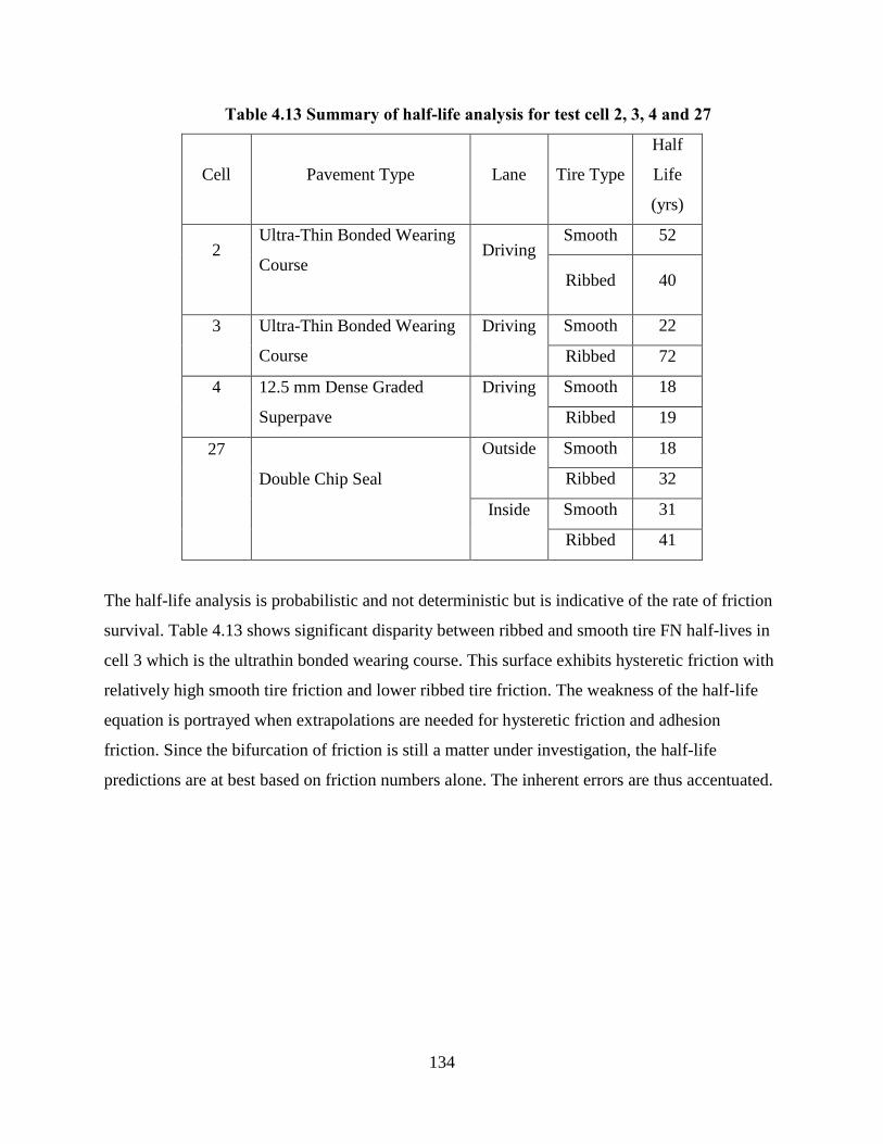
134
Table 4.13 Summary of half-life analysis for test cell 2, 3, 4 and 27
Cell Pavement Type Lane Tire Type
Half
Life
(yrs)
2
Ultra-Thin Bonded Wearing
Course
Driving
Smooth 52
Ribbed 40
3
Ultra-Thin Bonded Wearing
Course
Driving
Smooth 22
Ribbed 72
4
12.5 mm Dense Graded
Superpave
Driving
Smooth 18
Ribbed 19
27
Double Chip Seal
Outside
Smooth 18
Ribbed 32
Inside
Smooth 31
Ribbed 41
The half-life analysis is probabilistic and not deterministic but is indicative of the rate of friction
survival. Table 4.13 shows significant disparity between ribbed and smooth tire FN half-lives in
cell 3 which is the ultrathin bonded wearing course. This surface exhibits hysteretic friction with
relatively high smooth tire friction and lower ribbed tire friction. The weakness of the half-life
equation is portrayed when extrapolations are needed for hysteretic friction and adhesion
friction. Since the bifurcation of friction is still a matter under investigation, the half-life
predictions are at best based on friction numbers alone. The inherent errors are thus accentuated.

135
CHAPTER 5: CONCLUSION & RECOMMENDATIONS
136
CONCLUSION This report presents results of the research that was conducted on various asphalt pavement
surfaces in the MnROAD facility. Construction of Various Test Cells and initial monitoring
provided useful results Seasonal Measurements of surface was conducted and annual reports
were rendered as tasks of this project. However the 4th year performance and advanced data
analysis and results in addition to the construction and initial monitoring are reported in this final
report. It also discussed the fundamentals of surface profilometry, described the construction of
the textures and performance trends of the various surface parameters. The variables examined
include friction, measured with the lock wheel skid truck, smoothness, measured with the light
weight profiler, mean profile depth measured by the circular track meter, sound absorption
measured by the acoustic impedance tube and Tire-Pavement-Interaction-Noise measured by the
on board sound intensity device. All surface textures examined were isotropic in the micro and
macrotexture regimes although paving is in a given direction. This report performed advanced
data analysis and accentuated intrinsic relationships between important variables.
Construction of the test cells and monitoring for 4 years prior to advanced analysis
accentuated some notable trends. The research constructed different surface types with a wide
range of mix designs and materials in close proximity to each other, to provide a valuable insight
into the influence of mixture, environmental and traffic factors on various surface characteristics.
The following are general inferences and comparisons that can be made about the influence of
the mixture properties on the surface characteristics of the various mixture types at MnROAD.
• The porous asphalt mixtures (Cells 86 and 88) show a substantial amount of raveling,
which is most likely due to a combination of construction defects, snowplow damage,
and wear from heavy truck traffic.
• The largest rut depth on the Mainline is about ¼” while rut depths on the Low Volume
Road are approaching ½” on some cells.
• The 4.75 mm taconite mixture (Cell 106) showed the lowest rut depths, closely followed
by some of the dense graded mixtures (Cells 22, 24, and 87).
• The porous asphalt surfaces show the greatest rut depths.
137
• The UTBWC surfaces (Cells 2 and 3) are the smoothest over time. The porous asphalt
surfaces (Cells 86 and 88) are the roughest over time. Ride quality tends to be worst in
the spring with frozen or thawing conditions and better in the summer and fall when the
subgrade materials dry out.
• Aggressive, open graded surfaces (porous asphalt, chip seal, UTBWC) have the highest
mean profile depth, while the 4.75 mm taconite mixture has the lowest profile depth.
• Texture values can be variable when measured at different stations and offsets within a
cell.
• Friction numbers measured by the skid trailer were generally very good with the
exception of Cell 24, which has received a fog seal treatment just before friction
measurements the last three years. For the dense graded asphalt surfaces (Cells 4, 106,
19, 22, 24, and 87) the ribbed tire has significantly higher friction numbers than the
smooth tire. For the more open, aggressive asphalt surfaces (Cells 2, 3, 27, 86, and 88)
the ribbed and smooth tires give more similar values, with the smooth tire often
exhibiting a higher friction number. In general the passing/outside lane has a higher
friction number than the driving/inside lane, showing the effect of traffic on friction. The
UTBWC (Cell 3) and 4.75 mm taconite (Cell 106) surfaces had the highest coefficient
of friction values measured with the dynamic friction tester. The dense graded
Superpave surfaces (Cells 4, 19, and 22) had approximately equal coefficients. On Cell
24 the coefficient of friction decreased with each successive application of fog seal,
indicating that a light sanding or chip seal may be considered to maintain a safe driving
surface.
• The porous asphalt surfaces (Cells 86 and 88) are the quietest, while the chip seal (Cell
27) and some of the dense graded asphalt mixtures (Cells 4 and 24) are the loudest.
OBSI levels are lowest in the summer when the pavement surface is warm; they are
highest in cold weather. There is a general upward trend of noise levels over time with
the porous asphalt showing a more gradual trend and dense graded surfaces showing a
sharper increase. In some cases (e.g., NovaChip) the difference between cool and warm
weather results is remarkable, while in other cases (e.g. porous asphalt) the differences
in OBSI levels between seasons are much less.
138
• Porous asphalt surfaces (Cells 86 and 88) exhibited the highest sound absorption
coefficients; UTBWC surfaces (Cells 2 and 3) are a distant second. Dense graded
asphalt mixtures have extremely low sound absorption coefficients, with the 4.75 mm
taconite mixture (Cell 106) having the lowest. The sound absorption coefficients of the
open graded surface textures (porous and UTBWC) decrease significantly over time,
while this is not the case for the dense graded mixtures.
Advanced analysis accentuated some important findings.
OBSI- temperature correlation was found to be a negative polynomial relationship
indicating high importance of temperature to OBSI relationship in asphalt. It was
ascertained that texture mean profile depth was not as significant as texture skewness in
predicting surface properties. Additionally, the frictional time series appears to follow the
first order differential equation similar to half-life equation. Based on results obtained
from annual monitoring the asphalt surfaces were not associated with laser-induced
anomalous IRI reading errors.
Prior to this study, minimal reference to the skewness of asphalt surfaces was available.
This study examined the importance of skewness from the traffic data in relation to
friction and OBSI. This research showed that skewness or texture orientation is an
important variable in the prediction of asphalt surfaces. It shows that skewness when
compared to mean profile depth was a far better predictor of OBSI and friction than mean
profile depth.
Traffic difference was found to be a significant variable in the friction trend of the asphalt
surfaces when the low volume roads inside lane of the cells were compared to the
corresponding outside lane and the mainline driving and passing lanes of the cells
examined were compared in using the Wilcoxon Rank sum, Wilcoxon Sign Rank and the
T-test. A similar test on (OBSI -100dBA) found traffic to be insignificant within the 5
years of monitored performance of the same test tracks.
139
Prior to this study, minimal reference describing the rate of degradation of friction or skid
resistance of asphalt surfaces in relation to the skid resistance at the time of measurement
was available. This study finds the relationship to be similar to the half-life probabilistic
function. The half-life of the various texture types was therefore computed. This
describes the practical high rate of polishing or skid resistance reduction when the value
of skid is high. In pervious asphalt, degradation of the surface does not reduce frictional
resistance because raveling
RECOMMENDATIONS In the evaluation of asphalt surfaces, consideration should be given to texture orientation.
There is an effect of temperature on Tire-Pavement-Interaction-Noise of asphalt pavements. A correction algorithm based on the temperature correlation obtained in this research is recommended. In our current specification, as traffic levels increase, a more angular and durable aggregate is required. We vary PG grades by traffic conditions but it relates to rutting and cracking characteristics. Current specification may include a simple check for texture orientation to facilitate corrective action towards friction and noise without compromising other required characteristics.
Pervious asphalt shows good acoustic properties. Research should investigate a durability enhancement of porous asphalt for use as acoustic. In our current specification as traffic levels increase a more angular and durable aggregate is required. We vary PG grades by traffic conditions but it relates to rutting and cracking characteristics. Does this research provide any recommendations on how we should specify our materials based on skid resistance and noise. Since most of the observed delamination is associated with down drain, more viscous binders are recommended to minimize this phenomenon in pervious mixes.
Subsequent work on long-term performance should examine time series analysis so that the performance and seasonal trends will be built into the prediction / forecasting algorithm for OBSI, and ride quality.
140
REFERENCES
1. South African National Roads Agency. Pavement Management Site, accessed August 7,
2008. http://www.nra.co.za/live/content.php?Item_ID=185
2. Sandberg, U., Ejsmont, J. Tire Road Noise Reference Manual Informex. Handelsbolag Harg
SE 59040 Kisa, Sweden 2002.
3. Henry, J. Evaluation of Pavement Friction Characteristics. National Cooperative Highway
Research Program (NCHRP) Synthesis No. 291. Transportation Research Board, 2000,
Washington D.C.
4. Summer, C.J. The Idiot’s Guide to Highway Maintenance, accessed August 22, 2008.
<http://www.highwaysmaintenance.com/skidtext.htm>
5. Flintsch, G., Al-Qadi, A., McGhee, K., Davis, R. Effects of HMA Design Properties on
Pavement Surface Friction. Maintenance and Rehabilitation of Pavements and
Technological Control: Proceedings of the 3rd International Symposium. University of
Minho, Guimarães, Portugal, July 2003.
6. Cerezo, V., Gothie, M. Megatexture Measurement with a Non-Contact Profilometer:
Accuracy of the Method and Factors of Influence. Transportation Research Board Annual
Meeting, Washington, D.C., 2008.
7. “Calculating Pavement Macrotexture Profile Depth,” ASTM Standard Practice E-1845, IHS
online ASTM Standards, American Society for Testing and Materials, West Conshohocken,
PA, 2005.
8. The Study of Maintenance Repairs: The Effect of Maintenance on IRI Values. Unpublished
MnDOT Report, 1998.
9. International PIARC Experiment to Compare and Harmonize Texture and Skid Resistance
Measurements, PIARC Report 01.04.T, The World Road Association, Paris, 1995.
10. “Calculating the Friction Index of a Pavement Surface,” ASTM Standard Practice E-1960,
IHS online ASTM Standards, American Society for Testing and Materials, West
Conshohocken, PA, 2007.
11. “Skid Resistance of Paved Surfaces Using a Full Scale Tire,” ASTM Standard Practice E-
274, IHS online ASTM Standards, American Society for Testing and Materials, West
Conshohocken, PA, 2006.
141
12. “Measuring Pavement Macrotexture Depth Using a Volumetric Technique,” ASTM Standard
Practice E-965, IHS online ASTM Standards, American Society for Testing and Materials,
West Conshohocken, PA, 2006.
13. “Measuring Pavement Macrotexture Properties Using the Circular Track Meter,” ASTM
Standard Practice E-2157, IHS online ASTM Standards, American Society for Testing and
Materials, West Conshohocken, PA, 2006.
14. Smit, A., Waller, B. Evaluation of the Ultra-Light Inertial Profiler (ULIP) For Measuring
Surface Texture on Pavements. Federal Highway Administration. National Center for
Asphalt Technology, NCAT Report No. 07-01, June 2007, Auburn, Alabama.
15. Perera, R., Kohn, S., Soils and Materials Engineers, inc., Plymouth, MI. Issues in Pavement
Smoothness: A Summary Report. National Cooperative Highway Research Program,
Transportation Research Board, National Academies, Web Document No. 42 (20-51[1])
Contractor’s Final Report, March 2002.
16. Berengier, M., Anfosso-Ledee, F. State of the Art Prediction and Control of Road Traffic
Noise in France. Transportation Research Board of the National Academies, Transportation
Research Record 1629, pp. 71-77.
17. Descornet, G., Goubert, L. Noise Classification of Road Pavements. European Commission
Directorate General Environment, Task 1: Technical Background Information Draft Report,
June 2006.
18. Boscaino, G., Pratico, F.G., Vaiana, R. Texture Indicators and Surface Performance in
Flexible Pavements. Surf 2004, Fifth Symposium on Pavement Surface Characteristics, June
6-10, 2004, Toronto, Ontario, Canada.
19. Nagelhout, M., Wennink, P.M., Gerristen, W. Detection of Raveling. Surf 2004, Fifth
Symposium on Pavement Surface Characteristics, June 6-10, 2004, Toronto, Ontario,
Canada.
20. Izevbekhai, B. Report on Pavement Surface Characteristics Mini-Rodeo (MnDOT Test Data
and Data Comparison). Minnesota Department of Transportation, Unpublished Report,
2008.
21. Jackson, M. Measuring Pavement Friction Characteristics at Variable Speeds for Added
Safety. University of North Florida, Division of Engineering. Florida Department of
Transportation, FDOT Order # DO-51684, Final Report, July 2005.
142
22. Maurer, P. The Influence of Different Measuring Tires, Measuring Speed and Macrotexture
on Skid Resistance Measurements. Surf 2004, Fifth Symposium on Pavement Surface
Characteristics, June 6-10, 2004, Toronto, Ontario, Canada.
23. Khasawneh, M., Liang, R. Correlation Study Between Locked Wheel Skid Trailer and
Dynamic Friction Tester. Transportation Research Board Annual Meeting, Washington,
D.C., 2008.
24. De Roo, F., Gerretsen, E. Modelling of Acoustical Road Surface Characteristics with
RODAS (Road Design Acoustic Simulation). AIPCR/PIARC, 2000.
25. Lee, Y., Yurong, L., Ying, L., Fwa, T, Choo, Y. Skid Resistance Prediction by Computer
Simulation. Association of Asphalt Paving Technologists (AAPT), 2004.
26. Trifiro, F., Flintsch, G., Giovanni, G., de Leon, E., McGhee, K. Comparison of Friction
Measuring Devices and Preliminary Evaluation of the International Friction Index.
Transportation Research Board Annual Meeting, Washington, D.C., 2008.
27. McGhee, K., Flintsch, G., de Leon Izeppi, E. Using High Speed Texture Measurements to
improve the Uniformity of Hot-Mix Asphalt Pavements. Virginia Transportation Research
Council in cooperation with: U.S. Department of Transportation, FHWA, Final Report No.
VTRC 03-R12, May 2003.
28. Ongel, A., Kohler, E., Lu, Q., Harvey, J. Comparison of Surface Characteristics and
Pavement/Tire Noise of Various Thin Asphalt Overlays. Transportation Research Board
86th Annual Meeting, Washington, D.C., 2007.
29. A. Johnson, Clyne, T. R., Worel, B. J. “2008 MnROAD Phase II Construction Report”.
Minnesota Department of Transportation, June 2009.
30. “Measuring Pavement Macro texture Depth Using a Volumetric Technique,” ASTM
Standard Practice E-965, IHS online ASTM Standards, American Society for Testing and
Materials, West Conshohocken, PA, 2006.
31. “Measuring Pavement Macro texture Depth Using a Volumetric Technique,” ASTM
Standard Practice E-965, IHS online ASTM Standards, American Society for Testing and
Materials, West Conshohocken, PA, 2006.
32. “Measuring Pavement Macro texture Properties Using the Circular Track Meter,” ASTM
Standard Practice E-2157, IHS online ASTM Standards, American Society for Testing and
Materials, West Conshohocken, PA, 2006.
143
33. Abe, H., Henry, J.J., Tamari, A., Wambold, J. C., “Measurement of Pavement Macro texture
using Circular Texture Meter (CTMeter),” Transportation Research Board Annual Meeting,
Washington D.C., 2001.
34. Descornet, G., Goubert, L. Noise Classification of Road Pavements. European Commission
Directorate General Environment, Task 1: Technical Background Information Draft Report,
June 2006.
35. Henry, J. Evaluation of Pavement Friction Characteristics. National Cooperative Highway
Research Program (NCHRP) Synthesis No. 291. Transportation Research Board, 2000,
Washington D.C.
36. Izevbekhai, B. Report on Pavement Surface Characteristics Mini-Rodeo (MnDOT Test Data
and Data Comparison). Minnesota Department of Transportation, Unpublished Report,
2008.
37. Izevbekhai, B. “Report of Pavement Surface Characteristics Mini Rodeo (MnDOT Test Data
and Data Comparison)”. Minnesota Department of Transportation, Project MPR 6-(012) and
TPF 5-(134), July 2008.
38. “Skid Resistance of Paved Surfaces Using a Full Scale Tire,” ASTM Standard Practice E-
274, IHS online ASTM Standards, American Society for Testing and Materials, West
Conshohocken, PA, 2006.
39. Hanson, D, James, R., NeSmith, C. Tire/Pavement Noise Study. Sponsored by Federal
Highway Administration, National Center for Asphalt Technology, NCAT Report No. 04-02,
August 2004.
40. Johnson, A., Clyne, T. R., and B. J. Worel, 2008 MnROAD Phase II Construction Report,
Minnesota Department of Transportation, Final Report MN/RC 2009-22, 2009.
41. Watson, M., Clyne, T. R., Izevbekhai, B., and B. J. Worel, HMA Surface Characteristics
Related to Ride, Texture, Friction, Noise and Durability, Task 2 Report: Construction and
Initial Monitoring, Unpublished Report, Minnesota Department of Transportation, September
2009.
42. Watson, M., Clyne, T. R., Izevbekhai, B., and B. J. Worel, HMA Surface Characteristics
Related to Ride, Texture, Friction, Noise and Durability, Task 4 Report: First Year
144
Monitoring and Performance Report, Unpublished Report, Minnesota Department of
Transportation, June 2010.
43. Watson, M., Clyne, T., and B. Izevbekhai, HMA Surface Characteristics Related to Ride,
Texture, Friction, Noise, and Durability, Task 5 Report: Second Year Monitoring and
Performance Report, Unpublished Report, Minnesota Department of Transportation,
February 2011.
44. “Measuring Pavement Macro texture Properties Using the Circular Track Meter,” ASTM
Standard Practice E-2157, IHS online ASTM Standards, American Society for Testing and
Materials, West Conshohocken, PA, 2006.
45. Abe, H., Henry, J.J., Tamari, A., and J. C. Wambold, “Measurement of Pavement Macro
Texture using Circular Texture Meter (CTMeter),” Transportation Research Board Annual
Meeting, Washington D.C., 2001.
46. Surface Texture for Asphalt and Concrete Pavements, June 17, 2005. Federal Highway
Administration, http://www.fhwa.dot.gov/pavement/t504036.cfm, Accessed 2/29/2012.
47. “Concrete Texture Specifications” Minnesota Department of Transportation,
http://www.dot.state.mn.us/materials/concretedocs/texturespec.pdf, Accessed 2/29/2012.
48. “Standard Test Method for Measuring Skid Resistance of Paved Surfaces Using a Full-Scale
Tire,” ASTM Standard Practice E-274-06, IHS online ASTM Standards, American Society
for Testing and Materials, West Conshohocken, PA, 2006.
49. Technical Advisory: Pavement Friction Management, June 17, 2010. Federal Highway
Administration, http://www.fhwa.dot.gov/pavement/t504038.cfm, Accessed 2/29/2012.
50. D. Janisch, An Overview of MnDOT’s Pavement Condition Rating Procedures and Indices.
Minnesota Department of Transportation, Saint Paul, MN, May 2006.
51. B. I. Izevbekhai, Report of Pavement Surface Characteristics Mini Rodeo (MnDOT Test
Data and Data Comparison), Minnesota Department of Transportation, Project MPR 6-(012)
and TPF 5-(134), July 2008.
52. Descornet, G. and L. Goubert, Noise Classification of Road Pavements, European
Commission Directorate General Environment, Task 1: Technical Background Information
Draft Report, June 2006.
145
53. Miller, J. and W. Bellinger, Distress Identification Manual for the Long-Term Pavement
Performance Program (Fourth Revised Edition), Federal Highway Administration, FHWA-
RD-03-031, June 2003.
54. http://www.dot.state.mn.us/materials/pvmtmgmtdocs/Rating_Overview_State.pdf, Accessed
February 28, 2012.
55. http://www.dot.state.mn.us/materials/manuals/pvmtmgmt/distressmanual.pdf, Accessed
February 28, 2012.
56. Rutting, http://pavementinteractive.org/index.php?title=Rutting, Accessed February 28, 2012
57. Abe, H., Henry, J.J., Tamai, A., and Wambold, J.C., “Measurement of Pavement
Macrotexture Using the Circular Texture Meter (CTMeter),” Transportation Research Board
Annual Meeting, Washington DC, 2001.
58. Izevbekhai B.I. & Voller V.R. (2013): Development and validation of a tenable process for
quantifying texture spikiness for pavement noise prediction, International Journal of
Pavement Engineering, 14:2, 190-205
59. Bazlamit, Subhi M., and Reza, Farhad. “Changes in Asphalt Pavement Friction Components
and Adjustment of Skid Number for Temperature.” Journal of Transportation Engineering
131 (2005): 470-476

146
APPENDIX

APPENDIX A Mix Design Worksheets
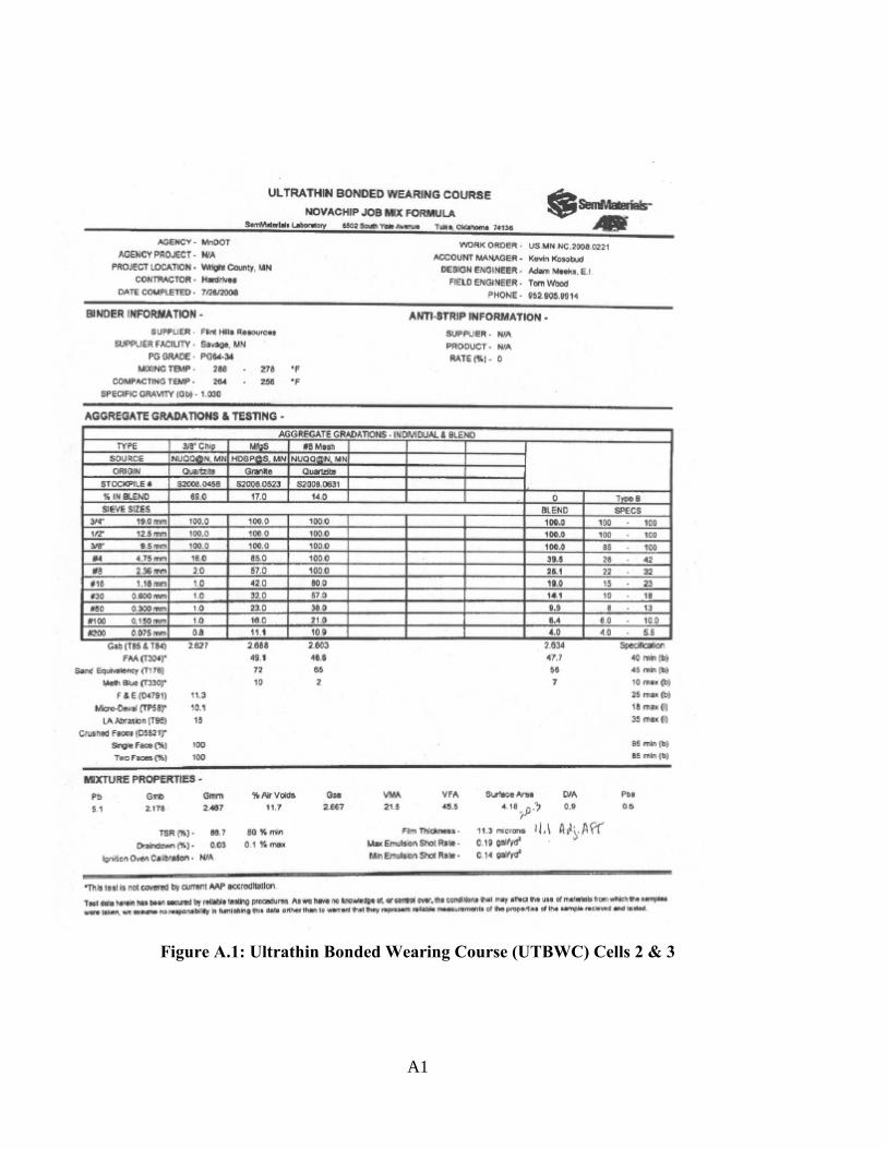
A1
Figure A.1: Ultrathin Bonded Wearing Course (UTBWC) Cells 2 & 3
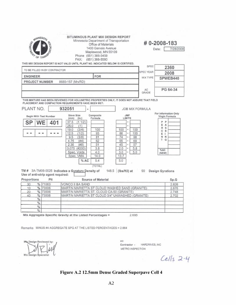
A2
Figure A.2 12.5mm Dense Graded Superpave Cell 4
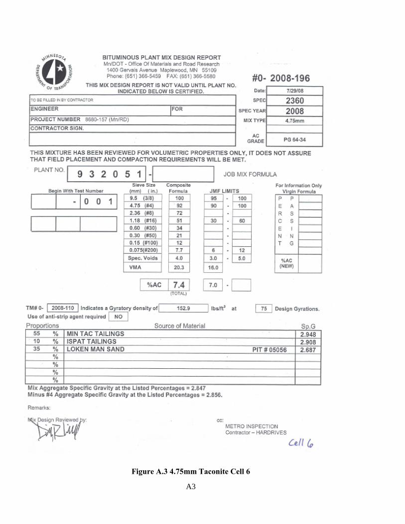
A3
Figure A.3 4.75mm Taconite Cell 6
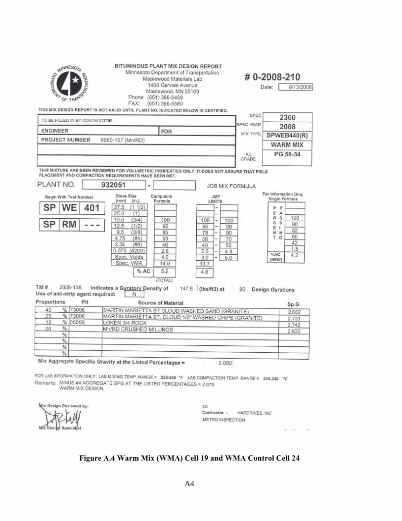
A4
Figure A.4 Warm Mix (WMA) Cell 19 and WMA Control Cell 24
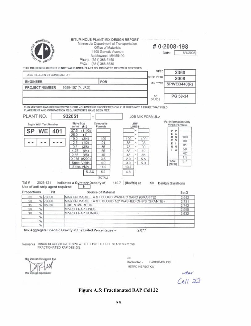
A5
Figure A.5: Fractionated RAP Cell 22
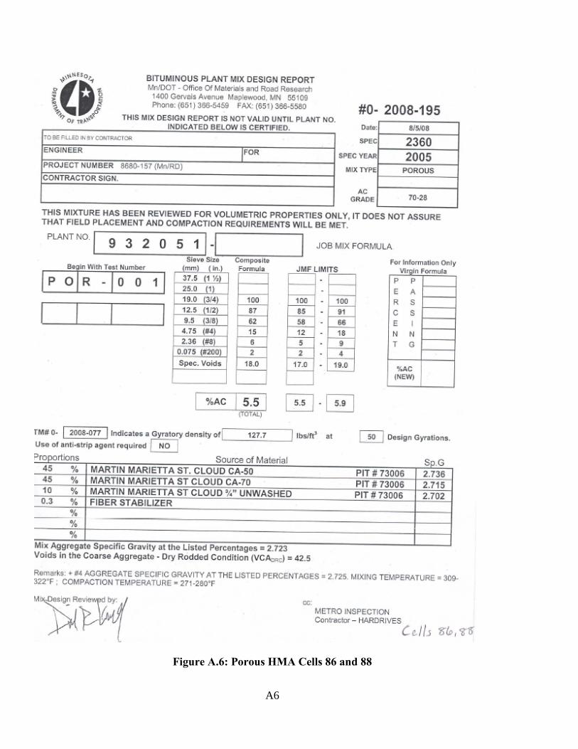
A6
Figure A.6: Porous HMA Cells 86 and 88
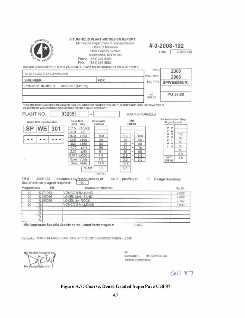
A7
Figure A.7: Coarse, Dense Graded SuperPave Cell 87

APPENDIX B Continuous Ride Plots
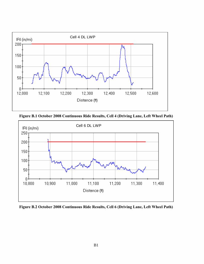
B1
Figure B.1 October 2008 Continuous Ride Results, Cell 4 (Driving Lane, Left Wheel Path)
Cell 4 DL LWP
Figure B.2 October 2008 Continuous Ride Results, Cell 6 (Driving Lane, Left Wheel Path)
Cell 6 DL LWP
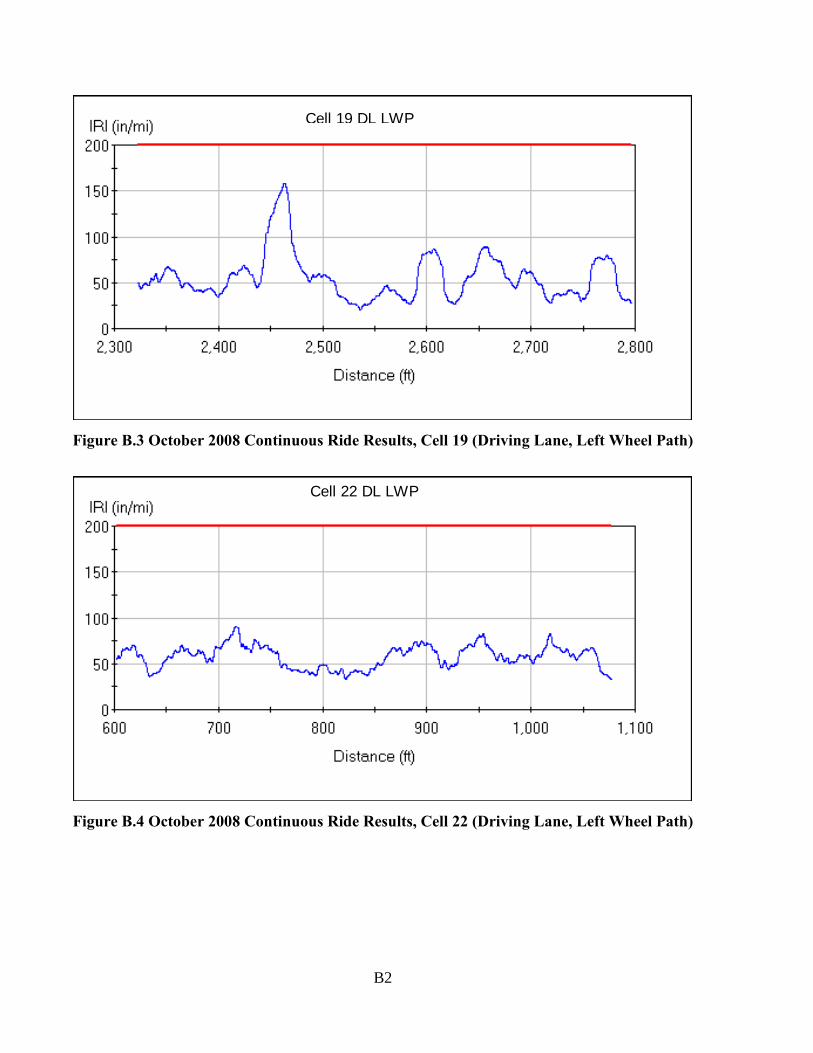
B2
Figure B.3 October 2008 Continuous Ride Results, Cell 19 (Driving Lane, Left Wheel Path)
Cell 19 DL LWP
Figure B.4 October 2008 Continuous Ride Results, Cell 22 (Driving Lane, Left Wheel Path)
Cell 22 DL LWP

APPENDIX C CT Meter Plots
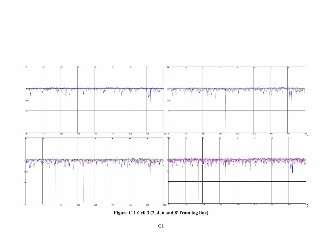
C1
Figure C.1 Cell 3 (2, 4, 6 and 8’ from fog line)
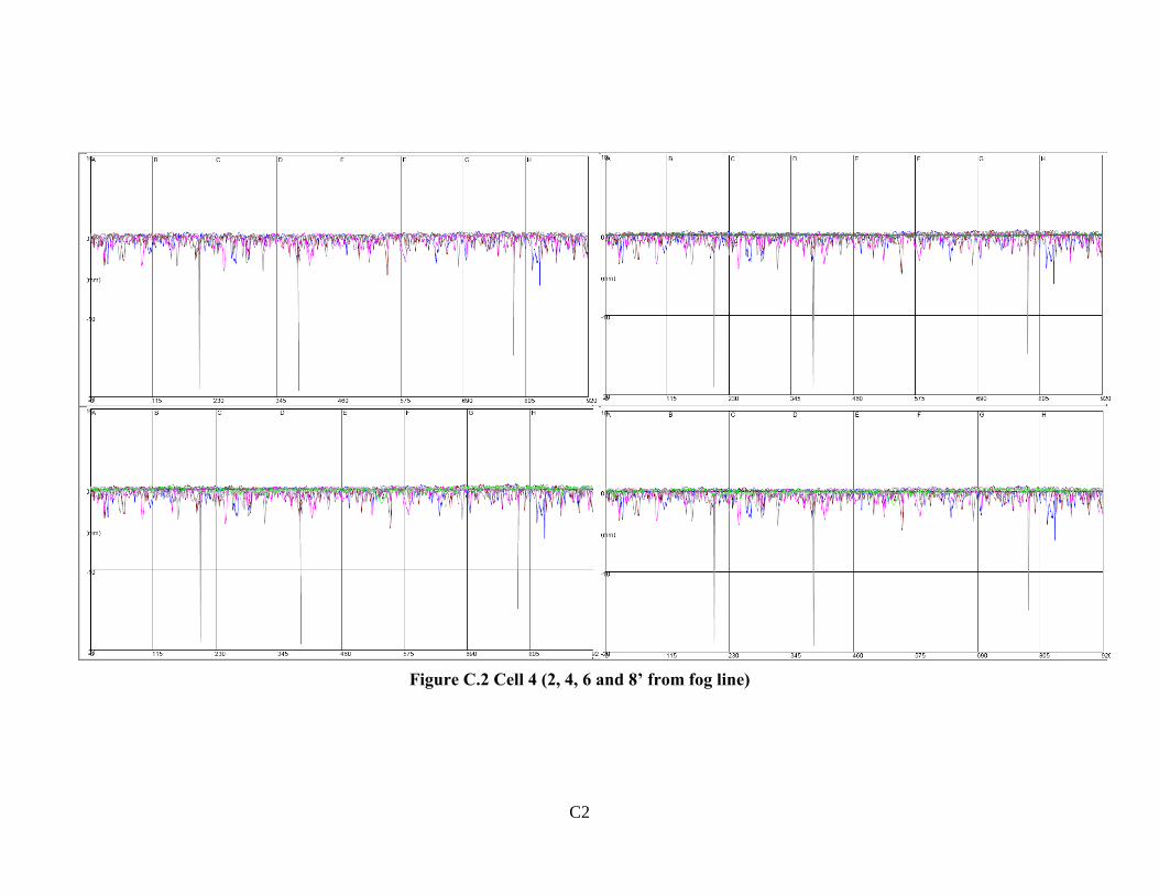
C2
Figure C.2 Cell 4 (2, 4, 6 and 8’ from fog line)
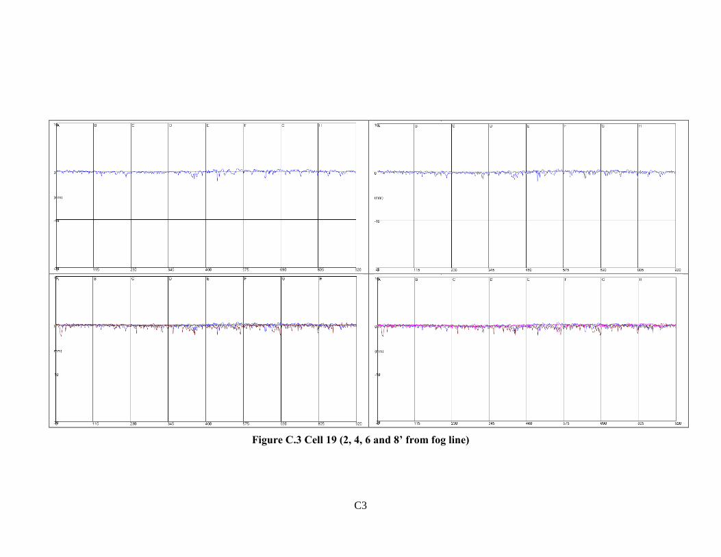
C3
Figure C.3 Cell 19 (2, 4, 6 and 8’ from fog line)
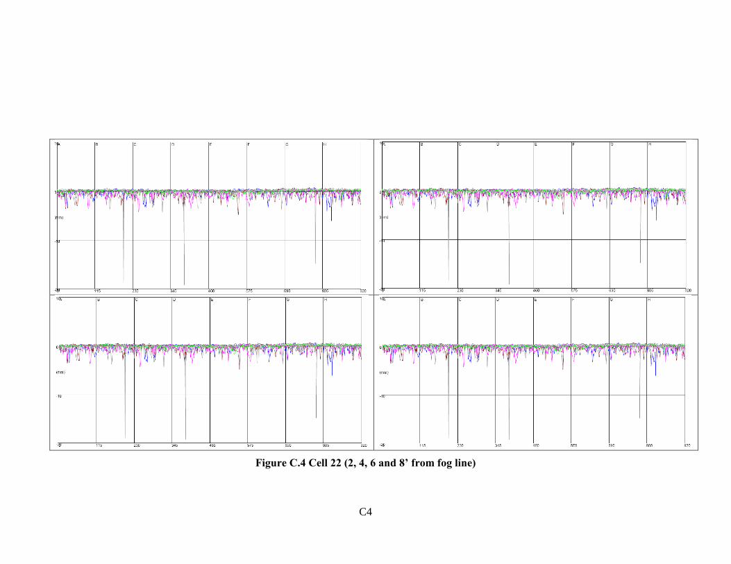
C4
Figure C.4 Cell 22 (2, 4, 6 and 8’ from fog line)
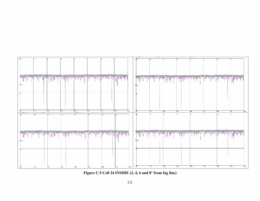
C5
Figure C.5 Cell 24 INSIDE (2, 4, 6 and 8’ from fog line)
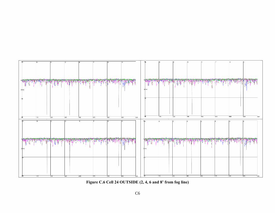
C6
Figure C.6 Cell 24 OUTSIDE (2, 4, 6 and 8’ from fog line)
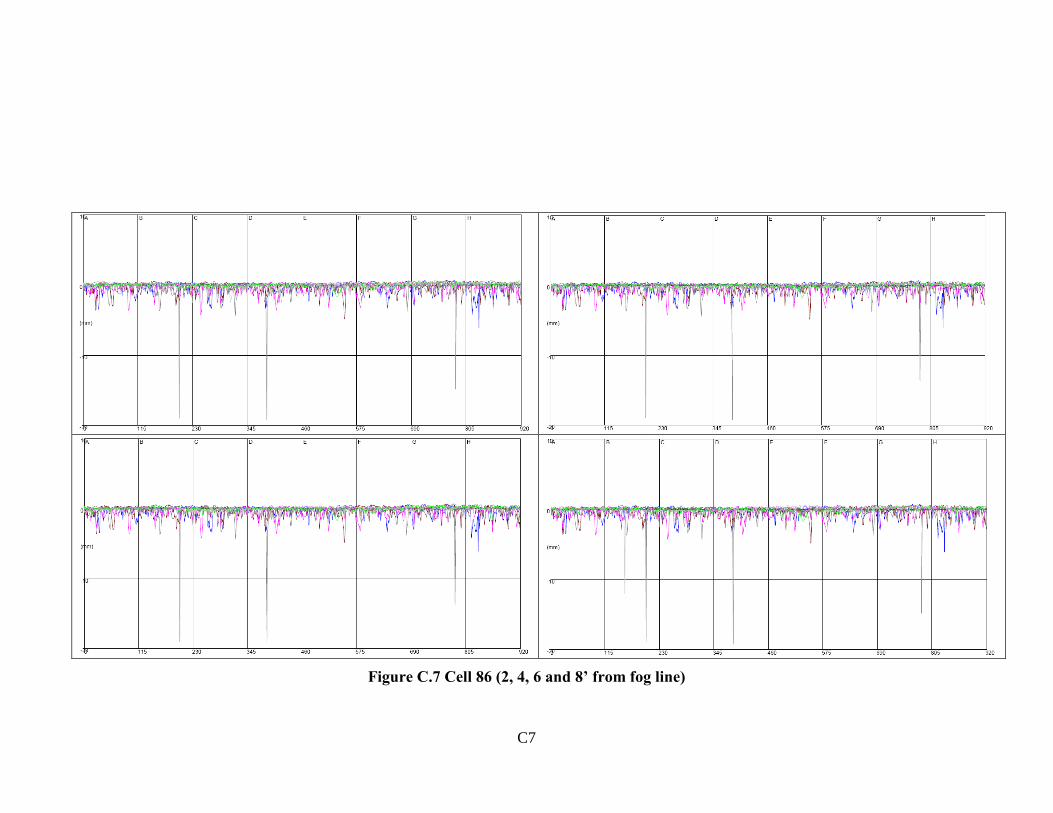
C7
Figure C.7 Cell 86 (2, 4, 6 and 8’ from fog line)

APPENDIX D OBSI Plot
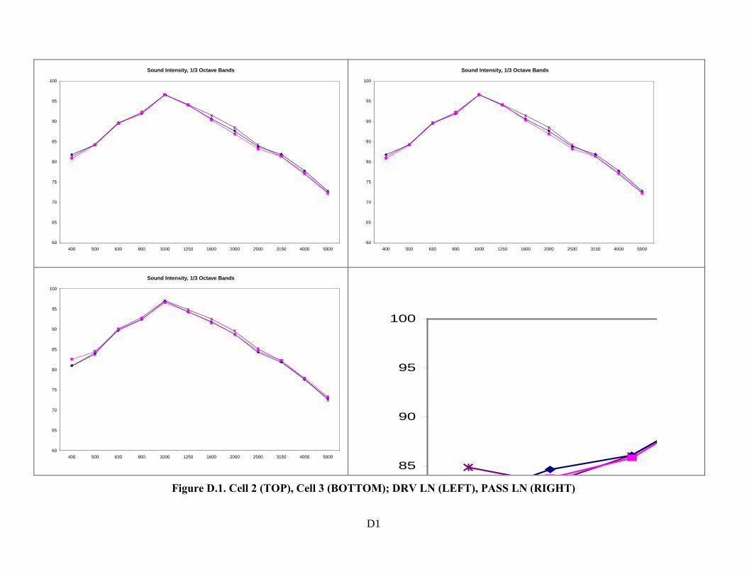
D1
Figure D.1. Cell 2 (TOP), Cell 3 (BOTTOM); DRV LN (LEFT), PASS LN (RIGHT)
Sound Intensity, 1/3 Octave Bands
60
65
70
75
80
85
90
95
100
400 500 630 800 1000 1250 1600 2000 2500 3150 4000 5000
Sound Intensity, 1/3 Octave Bands
60
65
70
75
80
85
90
95
100
400 500 630 800 1000 1250 1600 2000 2500 3150 4000 5000
Sound Intensity, 1/3 Octave Bands
60
65
70
75
80
85
90
95
100
400 500 630 800 1000 1250 1600 2000 2500 3150 4000 5000
85
90
95
100
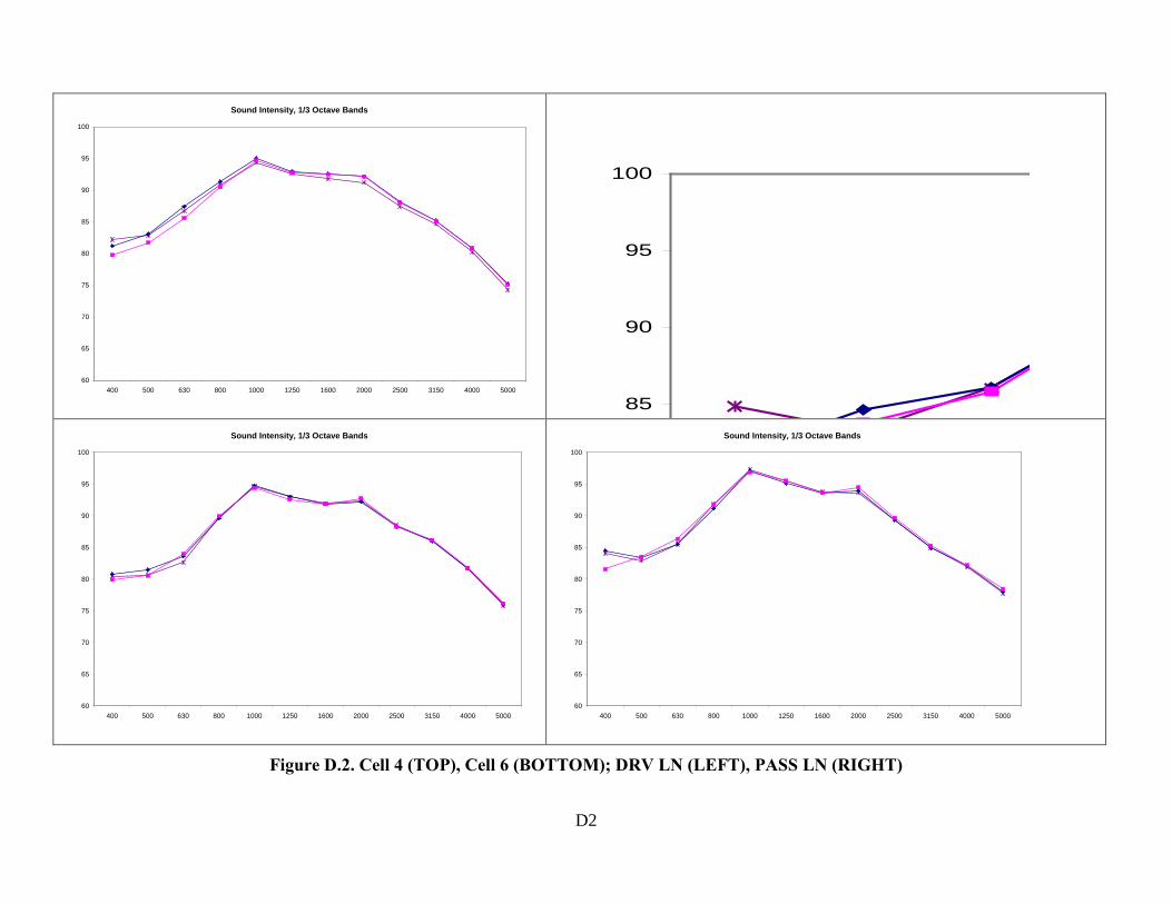
D2
Figure D.2. Cell 4 (TOP), Cell 6 (BOTTOM); DRV LN (LEFT), PASS LN (RIGHT)
Sound Intensity, 1/3 Octave Bands
60
65
70
75
80
85
90
95
100
400 500 630 800 1000 1250 1600 2000 2500 3150 4000 5000
85
90
95
100
Sound Intensity, 1/3 Octave Bands
60
65
70
75
80
85
90
95
100
400 500 630 800 1000 1250 1600 2000 2500 3150 4000 5000
Sound Intensity, 1/3 Octave Bands
60
65
70
75
80
85
90
95
100
400 500 630 800 1000 1250 1600 2000 2500 3150 4000 5000
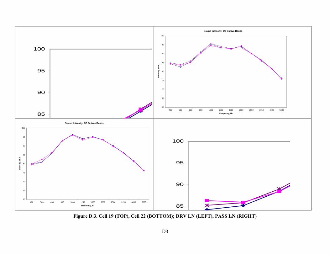
D3
Figure D.3. Cell 19 (TOP), Cell 22 (BOTTOM); DRV LN (LEFT), PASS LN (RIGHT)
85
90
95
100
Sound Intensity, 1/3 Octave Bands
60
65
70
75
80
85
90
95
100
400 500 630 800 1000 1250 1600 2000 2500 3150 4000 5000
Frequency, Hz
Inte
nsity
, dB
A
Sound Intensity, 1/3 Octave Bands
60
65
70
75
80
85
90
95
100
400 500 630 800 1000 1250 1600 2000 2500 3150 4000 5000
Frequency, Hz
Inte
nsity
, dB
A
85
90
95
100

APPENDIX E
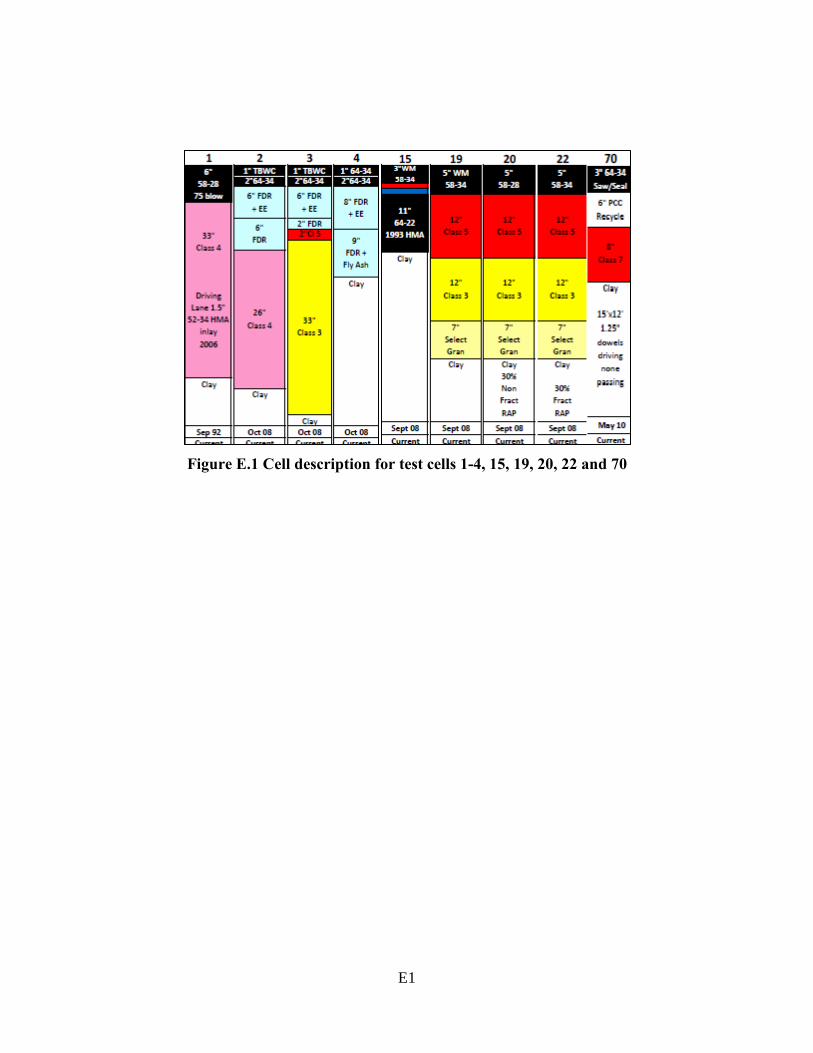
E1
Figure E.1 Cell description for test cells 1-4, 15, 19, 20, 22 and 70
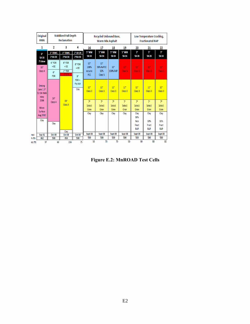
E2
Figure E.2: MnROAD Test Cells