geologic sequestration of carbon dioxide - united … sequestration of carbon dioxide draft...
TRANSCRIPT
Geologic Sequestration of Carbon Dioxide
Draft Underground Injection Control (UIC) Program Class VI Well Area of Review Evaluation and Corrective Action Guidance for Owners and Operators
March 2011

Office of Water (4606M) EPA 816-D-10-007 March 2011 http://water.epa.gov/drink
Draft UIC Program Class VI Well Area of i March 2011 Review Evaluation and Corrective Action Guidance
Disclaimer The Class VI injection well classification was established by the Federal Requirements under the Underground Injection Control Program for Carbon Dioxide Geologic Sequestration Wells (The GS Rule) (75 FR 77230, December 10, 2010). No previous EPA guidance exists for this class of injection wells. The Safe Drinking Water Act (SDWA) provisions and EPA regulations cited in this document contain legally-binding requirements. In several chapters this guidance document makes recommendations and offers alternatives that go beyond the minimum requirements indicated by the rule. This is done to provide information and recommendations that may be helpful for UIC Class VI program implementation efforts. Such recommendations are prefaced by the words “may” or “should” and are to be considered advisory. They are not required elements of the GS Rule. Therefore, this document does not substitute for those provisions or regulations, nor is it a regulation itself, so it does not impose legally-binding requirements on EPA, states, or the regulated community. The recommendations herein may not be applicable to each and every situation. EPA and state decision makers retain the discretion to adopt approaches on a case-by-case basis that differ from this guidance where appropriate. Any decisions regarding a particular facility will be made based on the applicable statutes and regulations. Mention of trade names or commercial products does not constitute endorsement or recommendation for use. EPA is taking an adaptive rulemaking approach to regulating Class VI injection wells, and the Agency will continue to evaluate ongoing research and demonstration projects and gather other relevant information as needed to refine the rule. Consequently, this guidance may change in the future without public notice. While EPA has made every effort to ensure the accuracy of the discussion in this document, the obligations of the regulated community are determined by statutes, regulations or other legally binding requirements. In the event of a conflict between the discussion in this document and any statute or regulation, this document would not be controlling. Note that this document only addresses issues covered by EPA’s authorities under the SDWA. Other EPA authorities, such as Clean Air Act (CAA) requirements to report carbon dioxide injection activities under the Greenhouse Gas Mandatory Reporting Rule (GHG MRR) are not within the scope of this document.
Draft UIC Program Class VI Well Area of ii March 2011 Review Evaluation and Corrective Action Guidance
Executive Summary EPA’s Federal Requirements Under the Underground Injection Control (UIC) Program for Carbon Dioxide Geologic Sequestration Wells has been codified in the US Code of Federal Regulations (40 CFR §146.81 et seq.), and is referred to as the Geologic Sequestration (GS) Rule. This GS Rule establishes a new class of injection well (Class VI) and sets minimum federal technical criteria for Class VI injection wells for the purposes of protecting underground sources of drinking water (USDWs). This document is part of a series of technical guidance documents that EPA is developing to support owners or operators of Class VI wells and the UIC Program permitting authorities.
The GS Rule requires owners or operators of Class VI injection wells to delineate the area of review (AoR) for the proposed Class VI well, which is the region surrounding the proposed well where underground sources of drinking water (USDWs) may be endangered by the injection activity [§146.84]. The GS Rule requires that the AoR be delineated using computational modeling and the AoR must be reevaluated periodically during the lifetime of the GS project [§146.84]. Within the AoR, the owners or operators must identify all potential conduits for fluid movement out of the injection zone, including both geologic features and artificial penetrations. The owner or operators must then evaluate those artificial penetrations that may penetrate the confining layer(s) of the injection project for the quality of casing and cementing, and in the case of abandoned wells, for the quality of plugging and abandonment, and perform corrective action on any identified artificial penetrations that could serve as a conduit for fluid movement. The GS Rule allows, at the discretion of the UIC Program Director, the use of ‘phased’ corrective action, where certain regions of the AoR are addressed prior to injection and other regions of the AoR are addressed during the injection-phase of the project [§146.84(b)(2)(iv)].
This guidance provides information regarding modeling requirements and recommendations for delineating the AoR, describes the circumstances under which the AoR is to be reevaluated, and describes how to perform an AoR reevaluation. In addition, the guidance presents information on how to identify, evaluate, and perform corrective action on artificial penetrations located within the AoR.
The introductory section reviews the definition of the AoR and regulations pertaining to AoR and Corrective Action in the GS Rule.
Section 2 addresses Computational Modeling of Geologic Sequestration.
Section 3 addresses AoR Delineation using Computational Models.
Section 4 addresses Identification, Evaluation, and Performing Corrective Action on Artificial Penetrations.
Section 5 addresses AoR Reevaluation.
Draft UIC Program Class VI Well Area of iii March 2011 Review Evaluation and Corrective Action Guidance
For each section, the Guidance: Explains how to perform activities necessary to comply with AoR and Corrective
Action requirements (e.g., performing computational modeling). Illustrative examples are provided in several cases.
Provides references to comprehensive reference documents and the scientific literature for additional information.
Explains how to report to the UIC Program Director the results of activities related to AoR and Corrective Action.
Draft UIC Program Class VI Well Area of iv March 2011 Review Evaluation and Corrective Action Guidance
Table of Contents Disclaimer ........................................................................................................................................ iExecutive Summary ........................................................................................................................ iiTable of Contents ........................................................................................................................... ivList of Figures ................................................................................................................................ viList of Tables ................................................................................................................................ viiAcronyms and Abbreviations ...................................................................................................... viiiDefinitions ...................................................................................................................................... ix
1. Introduction ............................................................................................................................. 11.1. Overview of the GS Rule AoR and Corrective Action Requirements ............................. 21.2. Organization of this Guidance .......................................................................................... 5
2. Computational Modeling for Geologic Sequestration ............................................................ 62.1. Basics of Computational Modeling .................................................................................. 6
2.1.1. Modeled Processes .................................................................................................... 92.1.2. Model Parameters ................................................................................................... 10
2.1.2.1. Intrinsic Permeability ...................................................................................... 132.1.2.2. Relative Permeability and Capillary Pressure ................................................. 152.1.2.3. Injection Rate ................................................................................................... 162.1.2.4. Mineral Precipitation Kinetic Parameters ........................................................ 172.1.2.5. Fluid Properties and Equations of State .......................................................... 192.1.2.6. Mass-Transfer Coefficients ............................................................................. 192.1.2.7. Model Orientation and Gridding Parameters ................................................... 19
2.1.3. Computational Approaches ..................................................................................... 202.1.3.1. Numerical Approaches .................................................................................... 202.1.3.2. Analytical, Semi-analytical, and Hybrid Approaches ..................................... 21
2.1.4. Model Uncertainty and Sensitivity Analyses .......................................................... 212.2. Existing Codes used for Development of GS Models .................................................... 22
3. AoR Delineation Using Computational Models ................................................................... 243.1. Data Collection and Compilation ................................................................................... 24
3.1.1. Site Hydrogeology .................................................................................................. 243.1.2. Operational Data ..................................................................................................... 25
3.2. Model Development ....................................................................................................... 263.2.1. Conceptual Model of the Proposed Injection Site .................................................. 263.2.2. Determination of Physical Processes to be Included in the Computational Model 263.2.3. Computational Model Design ................................................................................. 30
3.2.3.1. Computational Code Determination ................................................................ 303.2.3.2. Model Spatial Extent, Discretization, and Boundary Conditions .................... 303.2.3.3. Model Timeframe ............................................................................................ 303.2.3.4. Parameterization .............................................................................................. 31
3.2.4. Executing the Computational Model ...................................................................... 313.3. AoR Delineation Based on Model Results ..................................................................... 313.4. Reporting AoR Delineation Results to the UIC Program Director ................................ 38
Draft UIC Program Class VI Well Area of v March 2011 Review Evaluation and Corrective Action Guidance
4. Identifying Artificial Penetrations and Performing Corrective Action ................................. 404.1. Identifying Artificial Penetrations within the AoR ........................................................ 40
4.1.1. Historical Research ................................................................................................. 414.1.2. Site Reconnaissance ................................................................................................ 424.1.3. Aerial and Satellite Imagery Review ...................................................................... 434.1.4. Geophysical Surveys ............................................................................................... 43
4.1.4.1. Magnetic Methods ........................................................................................... 434.1.4.2. Electromagnetic Methods ................................................................................ 444.1.4.3. Ground Penetrating Radar ............................................................................... 47
4.2. Assessing Identified Abandoned Wells .......................................................................... 474.2.1. Abandoned Well Plugging Records Review ........................................................... 474.2.2. Abandoned Well Field Testing ............................................................................... 50
4.3. Performing Corrective Action on Wells Within the AoR .............................................. 524.3.1. Plugging of Wells within the AoR .......................................................................... 534.3.2. Remedial Cementing ............................................................................................... 54
4.4. Reporting Well Identification, Assessment, and Corrective Action to the UIC Program Director ............................................................................................................ 55
4.5. Use of Phased Corrective Action ................................................................................... 56
5. AoR Reevaluation ................................................................................................................. 585.1. Conditions Warranting an AoR Reevaluation ................................................................ 58
5.1.1. Minimum Fixed Frequency ..................................................................................... 585.1.2. Significant Changes in Operations .......................................................................... 585.1.3. Results from Site Monitoring that Differ From Model Predictions ........................ 595.1.4. Ongoing Site Characterization ................................................................................ 60
5.2. Performing an AoR Reevaluation .................................................................................. 605.2.1. Demonstrating Adequate Existing AoR Delineation .............................................. 605.2.2. Modifying the Existing AoR Delineation ............................................................... 67
5.2.2.1. Adjusting Site Conceptual Model .................................................................... 675.2.2.2. Model Calibration ............................................................................................ 675.2.2.3. Reporting a Revision to the AoR Computational Model ................................ 68
References ..................................................................................................................................... 70
Draft UIC Program Class VI Well Area of vi March 2011 Review Evaluation and Corrective Action Guidance
List of Figures
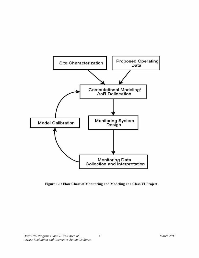
Figure 1-1: Flow Chart of Monitoring and Modeling at a Class VI Project ................................... 4
Figure 2-1: Equations of State for Carbon Dioxide ........................................................................ 8
Figure 2-2: Example Relative Permeability-Saturation and Capillary Pressure-Saturation Relationships for Water and Carbon Dioxide. Reproduced with kind permission of Springer Science + Business Media. ......................................................................... 18
Figure 3-1: Hypothetical Conceptual Site Model for Geologic Sequestration ............................. 28
Figure 3-2: Hypothetical Geologic Sequestration Site: Cross Sectional Schematic and Calculations ............................................................................................................... 34
Figure 3-3: Hypothetical Geologic Sequestration Site: Model Predicted Maximum Pressure Within the Injection Zone ......................................................................................... 35
Figure 3-4: Hypothetical Geologic Sequestration Site: Model Predicted Extent of Supercritical Carbon Dioxide Plume Over Time ............................................................................ 36
Figure 3-5: Hypothetical Geologic Sequestration Site: Initial Area of Review Based on Model Results ....................................................................................................................... 37
Figure 4-1: Total Field Aeromagnetic Map, Cook Creek Oil Field, Arcadia, Oklahoma ............ 46
Figure 4-2: Examples of Carbon Dioxide Leakage Through Improperly Abandoned Wells ....... 49
Figure 5-1: Hypothetical Geologic Sequestration Site: Comparison of Model Predictions and Plume Monitoring Results at 20 Years of Injection .................................................. 61
Figure 5-2: Hypothetical Geologic Sequestration Site: Comparison of Model Predictions and Pressure Monitoring Results at 20 Years of Injection ............................................... 62
Figure 5-3: Geologic Schematic of Frio Brine Pilot Project. The arrow at top indicates the north direction (from Doughty et al., 2007). Reproduced with kind permission of Springer Science + Business Media. ........................................................................................ 64
Figure 5-4: Observed and Modeled Carbon Dioxide Arrival at the Observation Well Based on Change in Fluid Density (from Doughty et al., 2007). Reproduced with kind permission of Springer Science + Business Media. .................................................. 65
Figure 5-5: Observed and Modeled Pressure Increase at (a) the Injection Well and (b) the Monitoring Well (from Doughty et al., 2007). Reproduced with kind permission of Springer Science + Business Media. ......................................................................... 65
Figure 5-6: Comparison of (a) Initial and (b) Post-Calibration Model Predictions of Carbon Dioxide Plume Evolution (from Ajo-Franklin et al., 2008) ...................................... 66
Figure 5-7: Hypothetical Geologic Sequestration Site: Initial AoR Delineation and Delineation after Reevaluation ..................................................................................................... 69

Draft UIC Program Class VI Well Area of vii March 2011 Review Evaluation and Corrective Action Guidance
List of Tables
Table 2-1: Model Parameters for Multiphase Fluid Modeling of Geologic Sequestration .......... 11
Table 4-1: Tools for Assessment of the Integrity of Abandoned Wells ....................................... 53
Draft UIC Program Class VI Well Area of viii March 2011 Review Evaluation and Corrective Action Guidance
Acronyms and Abbreviations 2D Two-Dimensional 3D Three-Dimensional AoR Area of Review API American Petroleum Institute AMSL Above Mean Sea Level ASTM American Society for Testing and Materials CASSM Continuous Active Seismic Source Monitoring CFR Code of Federal Regulations DOE United States Department of Energy EM Electromagnetic EPA United States Environmental Protection Agency GPR Ground Penetrating Radar GPS Global Positioning System GS Geologic Sequestration IR Infrared LBNL Lawrence Berkeley National Laboratory mD Millidarcy MESPOP Maximum Extent of Separate-phase Plume or Pressure Front mg/L Milligram per Liter MIT Mechanical Integrity Test MPa Megapascals NRC National Research Council Pa Pascals pH Potential for Hydrogen Ion Concentration PISC Post-Injection Site Care TDS Total Dissolved Solids UIC Underground Injection Control USDW Underground Source of Drinking Water USGS United States Department of the Interior, United States Geological Survey
Draft UIC Program Class VI Well Area of ix March 2011 Review Evaluation and Corrective Action Guidance
Definitions Area of review (AoR): The region surrounding the geologic sequestration project where USDWs may be endangered by the injection activity. The area of review is delineated using computational modeling that accounts for the physical and chemical properties of all phases of the injected carbon dioxide stream and displaced fluids, and is based on available site characterization, monitoring, and operational data as set forth in §146.84.
Boundary condition parameters: Parameters that describe fluid flow rates and/or pressures at the edges of the model domain and in the location of injection/extraction wells.
Capillary Pressure: The difference of pressures between two phases existing in a system of interconnecting pores or capillaries. The difference in pressure is due to the combination of surface tension and curvature in the capillaries.
Computational code: A series of interrelated mathematical equations solved by computer to represent the behavior of a complex system. For the purposes of GS, computational models represent, at a minimum, the flow and transport of multiple fluids and components in varying phases through porous media. Computational codes offer the ability to predict fluid flow in the subsurface using scientifically accepted mathematical approximations and theory. The use of computational codes is necessary because the mathematical formulations describing fluid flow are complicated and in many cases, non-linear. Several codes have been specifically developed or tailored for injection activities similar to GS, and can be used for this purpose.
Computational model: A mathematical representation of the injection project and relevant features, including injection wells, site geology, and fluids present. For a GS project, site specific geologic information is used as input to a computational code, creating a computational model that provides predictions of subsurface conditions, fluid flow, and carbon dioxide plume and pressure front movement at that site. The computational model comprises all model input and predictions (i.e., output).
Constitutive relationship: Typically empirically based approximations used to simplify the system and estimate unknowns in cases where the parameters of the governing equations are not readily available for use in the equation because necessary information is not typically measurable, and thus not directly input into the model. An example of a constitutive relationship is relative permeability-saturation functions. These functions estimate the relative permeability of a particular fluid in a porous media as a function of its saturation at a given location and time. This permeability is then used in the governing equation to predict flow.
Equation of state: An equation that expresses the equilibrium phase relationship between pressure, volume and temperature for a particular chemical species.
Geologic sequestration (GS): The long-term containment of a gaseous, liquid or supercritical carbon dioxide stream in subsurface geologic formations. This term does not apply to carbon dioxide capture or transport.
Draft UIC Program Class VI Well Area of x March 2011 Review Evaluation and Corrective Action Guidance
Geophysical surveys: The use of geophysical techniques (e.g., seismic, electrical, gravity, or electromagnetic surveys) to characterize subsurface rock formations.
Governing equation: The mathematical formulae that form the basis of the computational code are termed governing equations. For GS modeling, they ‘govern’ the predicted behavior of fluids in the subsurface provided by the code. Governing equations are mathematical approximations for describing flow and transport of fluids and their components in the environment.
Ground Penetrating Radar (GPR): A geophysical method that utilizes microwave technology in order to characterize features found in the subsurface.
Heterogeneity: Spatial variability in the geologic structure and/or physical properties of the site.
Hysteresis: The retardation in an effect after there has been a change in a system. An example of hysteresis is when flow into a system is stopped the pressure in the system does not drop instantly back to static conditions, but decreases slowly towards static conditions.
Immiscible: The property wherein two or more liquids or phases do not readily dissolve in one another.
Initial conditions: Parameter values at the start of the model simulation.
Intrinsic permeability: A parameter that describes properties of the subsurface that impact the rate of fluid flow. Larger intrinsic permeability values correspond to greater fluid flow rates. Intrinsic permeability has units of area (distance squared).
Model calibration: Adjusting model parameters in order to minimize the difference between model predictions and monitoring data at the site.
Multiphase flow: Flow in which two or more distinct phases are present (e.g., liquid, gas, supercritical fluid).
Numerical Artifacts: Model results that are created erroneously based on computational limitations of the model, which may result from improper model development.
Parameter: A mathematical variable used in governing equations, equations of state, and constitutive relationships. Parameters describe properties of the fluids present, porous media, and fluid sources and sinks (e.g., injection well). Examples of model parameters include intrinsic permeability, fluid viscosity, and fluid injection rate.
Relative permeability: A factor, between 0 and 1, that is multiplied by the intrinsic permeability of a formation to compute the effective permeability for a fluid in a particular pore space. When immiscible fluids (e.g., carbon dioxide, water) are present within the pore space of a formation, the ability for flow of those fluids is reduced, due to the blocking effect of the presence of the other fluid. This reduction is represented by relative permeability.
Sensitivity Analyses: The study of how the output of a model varies based in changes to an input variable or model parameter over a specified range of values. The results of a sensitivity

Draft UIC Program Class VI Well Area of xi March 2011 Review Evaluation and Corrective Action Guidance
analysis determine which input variable and model parameter variability have the greatest effect on the model results.
Stochastic Methods: The use of probability statistical methods in development of one or more possible realizations of the spatial patterns of the value(s) of a given set of model parameters.
Underground Injection Control Program: The program EPA, or an approved state, is authorized to implement under the Safe Drinking Water Act (SDWA) responsible for regulating the underground injection of fluids. This includes setting the minimum federal requirements for construction, operation, permitting, and closure of underground injection wells.
Underground source of drinking water (USDW): An aquifer or portion of an aquifer that supplies any public water system or that contains a sufficient quantity of ground water to supply a public water system, and currently supplies drinking water for human consumption, or that contains fewer than 10,000 mg/L total dissolved solids and is not an exempted aquifer.
Draft UIC Program Class VI Well Area of 1 March 2011 Review Evaluation and Corrective Action Guidance
1. Introduction
Area of review (AoR) evaluations and corrective action are long-standing permit requirements of the Underground Injection Control (UIC) Program of the U.S. Environmental Protection Agency (US EPA). The AoR refers to the delineated region surrounding the injection well(s) wherein the potential exists for underground sources of drinking water (USDWs) to be endangered by the leakage of injectate and/or formation fluids. Typically, for injection well classes other than Class VI, the AoR is defined as either a fixed radius around the injection well, or by a relatively simple radial calculation. Owners or operators of injection wells are required to identify any potential conduits for fluid movement, including artificial penetrations (e.g., abandoned wellbores) within the AoR, assess the integrity of any artificial penetrations, and perform corrective action where necessary to prevent fluid movement into a USDW.
The GS Rule introduces enhanced AoR and corrective action requirements for Class VI injection wells that are tailored to the unique circumstances of geologic sequestration of carbon dioxide (GS) projects [§146.84]. The purpose of this guidance is to identify appropriate methods for delineating the AoR and performing corrective action for Class VI injection wells. The intended primary audiences of this guidance document are Class VI injection well owners and operators and their representatives conducting AoR delineation modeling or performing artificial penetration identification, assessment, and corrective action activities. The UIC Program staff who are responsible for reviewing and approving Class VI injection well permit applications and related reports concerning AoR delineation and corrective action are another intended audience of this guidance document.
This document is one of a series of four technical guidance documents intended to provide information and possible approaches for addressing various aspects of permitting and operating a UIC Class VI injection well. There are three companion draft guidance documents that focus on site characterization, well construction, and testing and monitoring:
Geologic Sequestration of Carbon Dioxide: Draft Underground Injection Control (UIC)
Program Class VI Well Site Characterization Guidance for Owners and Operators. Geologic Sequestration of Carbon Dioxide: Draft Underground Injection Control (UIC)
Program Class VI Well Construction Guidance for Owners and Operators. Geologic Sequestration of Carbon Dioxide: Draft Underground Injection Control (UIC).
Program Class VI Well Testing and Monitoring Guidance for Owners and Operators (this guidance is under development and will be available in the near future).
These draft guidance documents are intended to complement each other and to assist owners and operators in preparing permit applications that satisfy the requirements of the GS Rule. Class VI injection well regulations are tailored to the characteristics of individual sites. For example, the required site characterization data collected will inform the model development for AoR delineation, and AoR models will be reevaluated, and perhaps change, based on the results of site testing and monitoring data (See Figure 1-1, of this guidance document, below). Cross-linkages between guidance documents are noted in the text where appropriate. Additional guidance on developing, presenting, and using the required Class VI project plan information as part of a
Draft UIC Program Class VI Well Area of 2 March 2011 Review Evaluation and Corrective Action Guidance
Class VI injection well permit application is provided in the draft project plan development guidance:
Geologic Sequestration of Carbon Dioxide: Draft Underground Injection Control (UIC)
Program Class VI Well Project Plan Development Guidance for Owners and Operators.
1.1. Overview of the GS Rule AoR and Corrective Action Requirements
An overview of the GS Rule requirements for Class VI injection wells is presented in this section. Details for all the requirements briefly described here are presented in later sections of this guidance. The GS Rule defines the AoR as “the region surrounding the GS project where USDWs may be endangered by the injection activity” [§146.84(a)]. USDWs in the vicinity of a proposed Class VI injection well may be endangered by (1) movement of carbon dioxide into the USDW, impairing drinking water quality through changes in pH, contamination by trace impurities in the injectate (e.g., mercury, hydrogen sulfide), and leaching of metals and/or organics; and (2) movement of non-potable water (e.g., brine) out of the injection formation into a USDW as caused by elevated formation pressures induced by injection. Therefore, the AoR encompasses the region overlying the extent of separate-phase (e.g., supercritical, liquid or gaseous) carbon dioxide migration, and the region overlying the extent of fluid pressure increase great enough to force fluids into any USDW.
The GS Rule requires that “the AoR is delineated using computational modeling that accounts for the physical and chemical properties of all phases of the injected carbon dioxide stream and is based on available site characterization, monitoring, and operational data” [§146.84(a)]. As discussed below, GS computational modeling for Class VI injection wells is more complex than methods used to delineate the AoR for other injection well classes in the UIC program. Additionally, the AoR must be reevaluated (a) periodically, at least once every five years, (b) when actual operational data differ significantly from initial estimated operational values that were used for model inputs, or (c) when monitoring data and model results differ significantly [§146.84(e)]. The purpose of Class VI injection well AoR reevaluation is to ensure that site monitoring data is used to update modeling results, and that the AoR delineation reflects any changed in operational conditions. The general relationship between site characterization, modeling, and monitoring activities at a GS project is given in Figure 1-1.
EPA anticipates that, in most cases, multiple injection wells will be operated within a single GS project. An individual UIC Class VI injection well permit must however be obtained separately for each injection well, as area permits are not allowed under the GS Rule [§144.33]. Nevertheless, if approved by the UIC Program Director, AoR delineation and corrective action activities may be performed comprehensively for all wells included within a single project. In all cases, EPA recommends that AoR delineation models account for all wells injecting carbon dioxide into the injection zone, including any injection wells associated with other UIC well class injection projects.
The corrective action requirements are generally similar for Class VI and the other existing injection well classes. However, due to the potentially large AoR at GS sites, EPA has allowed the use of phased corrective action, if approved by the UIC Program Director
Draft UIC Program Class VI Well Area of 3 March 2011 Review Evaluation and Corrective Action Guidance
[§146.84(b)(2)(iv)]. Phased corrective action would allow the owners or operators to perform corrective action only on a subset of artificial penetrations located within the AoR prior to injection that are located in regions nearest the injection well(s). Corrective action would continue during injection in the remaining regions of the AoR prior to carbon dioxide migration or pressure elevation in that area.
As a part of a Class VI injection well permit application, the owner or operator must submit an AoR and Corrective Action Plan that describes the anticipated activities that will be performed to comply with these requirements [§146.84(b)]. The AoR and Corrective Action Plan is approved by the UIC Program Director prior to submittal of the initial AoR delineation, and issuance of a permit [§146.84(b)]. This plan will facilitate dialogue between the owners or operators and the UIC Program Director to ensure that the UIC Program Director understands and agrees with methods that will be used for AoR delineation and corrective action. EPA recommends that the Class VI AoR and Corrective Action Plan include the following information:
1. The method for delineating the AoR, including the model to be used, assumptions that
will be made, and the site characterization data on which the model will be based;
2. The minimum fixed frequency, at least once every five (5) years, that the owner or operator proposes to reevaluate the AoR;
3. The monitoring and operational conditions that would warrant a reevaluation of the AoR prior to the next routinely scheduled reevaluation;
4. How monitoring and operational data (e.g., injection rate and pressure) will be used to inform an AoR reevaluation;
5. How corrective action will be conducted, including what corrective action will be performed prior to injection and what, if any, portions of the area of review will have corrective action addressed on a phased basis and how the phasing will be determined; how corrective action will be adjusted if there are changes in the area of review, and;
6. How site access will be guaranteed for future corrective action.
The requirements related to the AoR and Corrective Action Plan are discussed in depth in the Draft UIC Program Class VI Well Project Plan Development Guidance.
Draft UIC Program Class VI Well Area of 4 March 2011 Review Evaluation and Corrective Action Guidance
Figure 1-1: Flow Chart of Monitoring and Modeling at a Class VI Project
Draft UIC Program Class VI Well Area of 5 March 2011 Review Evaluation and Corrective Action Guidance
1.2. Organization of this Guidance
This guidance document is organized to generally follow the sequence of AoR and corrective action activities that an owner or operator will perform over time at a permitted Class VI injection well site. These activities will generally proceed as follows:
1. Collection of relevant site characterization and operational data [§§146.82(a)(3),
146.82(a)(7), and 146.83);
2. Development of an AoR and Corrective Action Plan [§§146.82(a)(13) and146.84(b)];
3. Performing AoR modeling and delineation [§146.82 (c)(1)];
4. Identification and assessment of artificial penetrations within the AoR [§§146.82 (a)(4) and 146.84(c)(2)];
5. Performing corrective action on those penetrations that may serve as a conduit for fluid movement [§§146.82 (c)(6) and 146.84(d)], and;
6. Reevaluation of the AoR periodically, at least once every five (5) years [§§146.82 (c)(9) and146.84(e)].
Activities (1) through (4) must be performed prior to receiving approval to inject carbon dioxide, and must be submitted to the UIC Program Director with the Class VI injection well permit application. The remaining activities will be performed after a permit application has been approved by the UIC Program Director and the Class VI injection well is actively operating.
This guidance document generally focuses on activities (3) to (6). Site characterization activities (activity 1) are discussed briefly in this guidance (Section 3.1), and are covered in more detail in the Draft UIC Program Class VI Well Site Characterization Guidance. Preparation of the AoR and Corrective Action Plan (activity 2) is also discussed briefly herein, and is discussed in more detail in the Draft UIC Program Class VI Well Project Plan Development Guidance. Section 2 of this guidance provides necessary background in computational modeling of geologic sequestration, and Section 3 discusses performing computational modeling in order to delineate the AoR and comply with permit requirements (activity 3). Section 4 of this guidance focuses on abandoned well identification, assessment, and corrective action within the AoR (activities 4 and 5). Lastly, Section 5 focuses on reevaluation of the AoR (activity 6).
Draft UIC Program Class VI Well Area of 6 March 2011 Review Evaluation and Corrective Action Guidance
2. Computational Modeling for Geologic Sequestration
The AoR for a Class VI injection project must be delineated using a computational model [§146.84(a)]. A computational model is a mathematical representation of the GS project and relevant features, including injection wells, site geology, and fluids present. As described below, a site-specific computational model is designed by incorporating the GS site and operational characteristics into a computational code, which is a computer program that has been designed to simulate multiphase flow and other pertinent processes in geologic media based on scientific principles and accepted mathematical equations.
Computational codes that may be used for modeling of GS are necessarily more technically complex than commonly used ground water flow codes because GS modeling considers multiphase flow of several immiscible fluids (i.e., ground water, carbon dioxide), phase changes of carbon dioxide, heat flow, and significant pressure changes. Furthermore, in some cases models consider reactive transport (e.g., chemical reactions between constituents) and geomechanical processes (e.g., induced fault activation). As discussed below, the GS Rule requires that the AoR be delineated using models that include multiphase flow, but not necessarily reactive transport or geomechanical processes. However, inclusion of these processes in the AoR delineation model may be important in some cases, and may be required by the UIC Program Director.
Several codes are available that are capable for use in development of adequate models for delineation of the AoR at a GS site and for complying with Class VI injection well permit requirements (Section 2.3). Although available codes are sophisticated and based on the best-available scientific understanding, computational models are never a perfect representation of reality, and cannot provide a completely accurate prediction of fluid movement at a GS site. For this reason, EPA recommends that model uncertainty be characterized and computational modeling is required to be complemented with required site monitoring [§146.84(e)]. When necessary (e.g., during AoR reevaluation), models may be calibrated to minimize differences between site monitoring data and model simulations.
This section discusses the fundamentals of computational modeling of GS in order to provide the necessary background for owners and operators, and to assist in understanding and complying with the GS Rule. Available modeling research studies have provided valuable information on the capabilities of available models, what information may be collected in order to properly inform model development, and how the model results may be presented.
2.1. Basics of Computational Modeling
There is a long history of simulating multiphase flow and transport in porous media using computational models. Comprehensive reviews of multiphase modeling are provided elsewhere (e.g., Miller et al., 1998; Gerritsen and Durlofsky, 2005; Finsterle, 2004). These models solve a series of governing equations to predict the composition and volumetric fraction of each phase state (e.g., liquid, gas, supercritical fluid) as a function of space and time for a particular set of circumstances. Governing equations are formulated to describe the flow and transport of several chemical species in several phases, in which interphase mass transfer may be important.
Draft UIC Program Class VI Well Area of 7 March 2011 Review Evaluation and Corrective Action Guidance
Typically, flow equations are derived by substituting a multiphase form of Darcy’s Law into continuum balance expressions.
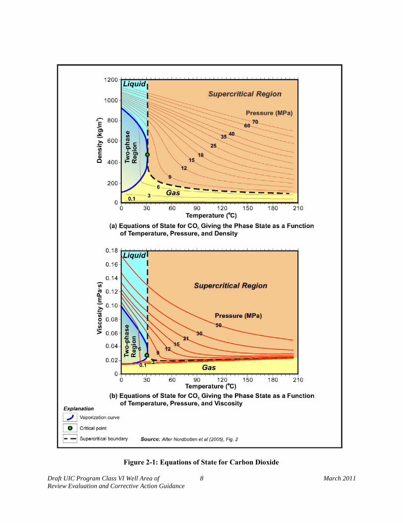
The solution of the continuum balance equations requires that they be supplemented with closure relations that express unknowns in terms of accessible parameters. These include equations of state and constitutive relationships. Equations of state express the equilibrium phase relationship between pressure, volume, and temperature for a particular chemical. Accepted equations of state for carbon dioxide are presented in Figure 2-1, and are discussed in Section 2.1.2.5. Constitutive relationships are typically empirically based approximations used to simplify the system and estimate unknowns. Examples of constitutive relationships are saturation-relative permeability relationships, interphase mass transfer relations, and solution reaction relations.
Draft UIC Program Class VI Well Area of 8 March 2011 Review Evaluation and Corrective Action Guidance
Figure 2-1: Equations of State for Carbon Dioxide
Draft UIC Program Class VI Well Area of 9 March 2011 Review Evaluation and Corrective Action Guidance
2.1.1. Modeled Processes
Computational codes used for GS vary in complexity, and may include routines for multiphase flow, reactive transport, and geomechanical processes. Traditionally, codes have been developed as separate entities to simulate these processes. Present-day simulators typically address and couple a subset of these processes. This is especially true for the coupling of geomechanical processes with multiphase flow or geochemical processes. However, robust simulation of GS may require interactive coupling of all three processes. The GS Rule only requires that multiphase flow be included in computational modeling. However, the owner or operator, or UIC Program Director, may determine that reactive transport and/or geomechanical modeling additionally be included for a particular proposed project. For example, reactive transport could be relevant if permeability and/or porosity are predicted to change as a result of precipitation/dissolution reactions. Geomechanical processes could be relevant if pressure and stress changes hydrogeologic properties.
Codes used to simulate multiphase flow generally incorporate some or all of the following processes: phase transition behavior of carbon dioxide (gas, liquid, supercritical fluid) and associated buoyancy; dissolution of carbon dioxide in brine and oil and associated increased density; dissolution of water in carbon dioxide; variable viscosity and density of brine and carbon dioxide phases; thermal effects such as cooling or freezing due to carbon dioxide expansion from supercritical and liquid phases; and reduced fluid permeability due to the presence of several immiscible fluids within a pore space.
Codes used to simulate reactive transport generally incorporate rate-limited intra-aqueous reactions, mineral dissolution and precipitation, changes in porosity and permeability due to these reactions, and multi-component gas mixtures. Reactive transport models can be used to determine the impact of carbon dioxide and its co-injectates (e.g., hydrogen sulfide, sulfur dioxide) on aquifer acidification, the concomitant mobilization of metals, and any mineral trapping of carbon dioxide (e.g., precipitation of carbonate minerals). Reactive transport models can also be used to assess corrosion of well construction materials as influenced by carbon dioxide.
The length scales associated with interfacial geochemistry are very small (e.g., micrometers to millimeters) compared to multiphase flow simulation (meters to kilometers). Small grid spacing around these regions may imply associated small time steps, so that the overall problem becomes computationally demanding when trying to couple these reactions to multiphase flow. Data related to geochemical rate parameters are generally lacking (e.g., Knauss et al., 2005; Xu et al., 2006), and have to be estimated for a wide range of possible environmental conditions and mineralogical interfaces. Several common codes that may be used for AoR delineation, such as ECLIPSE, normally do not include routines for reactive transport.
Geomechanical codes can be used to evaluate the effect of reservoir pressurization and buoyancy on the integrity of geologic confining units, reactivation of existing fractures and faults, and rock properties such as porosity and permeability. The amount and spatial distribution of pressure buildup in a geologic formation will depend on the rate of injection, the permeability and
Draft UIC Program Class VI Well Area of 10 March 2011 Review Evaluation and Corrective Action Guidance
thickness of the injection formation, mechanistic properties of the rock matrix, the permeability of the confining units, and the presence or absence of permeability barriers, and boundary conditions of the system. Models used to simulate geomechanical processes generally incorporate effective stress/strain relationships, aperture stiffness and associated closing and widening, and variation in porosity and permeability. Geomechanical modeling may require simulation on both a large and small scale (individual fractures), which can be computationally challenging (i.e., require long model processing times on the order of days). When individual fractures are considered, the spatial grid resolution has to be on the order of meters or less. Therefore, smaller-domain models may be necessary to investigate migration through individual fractures.
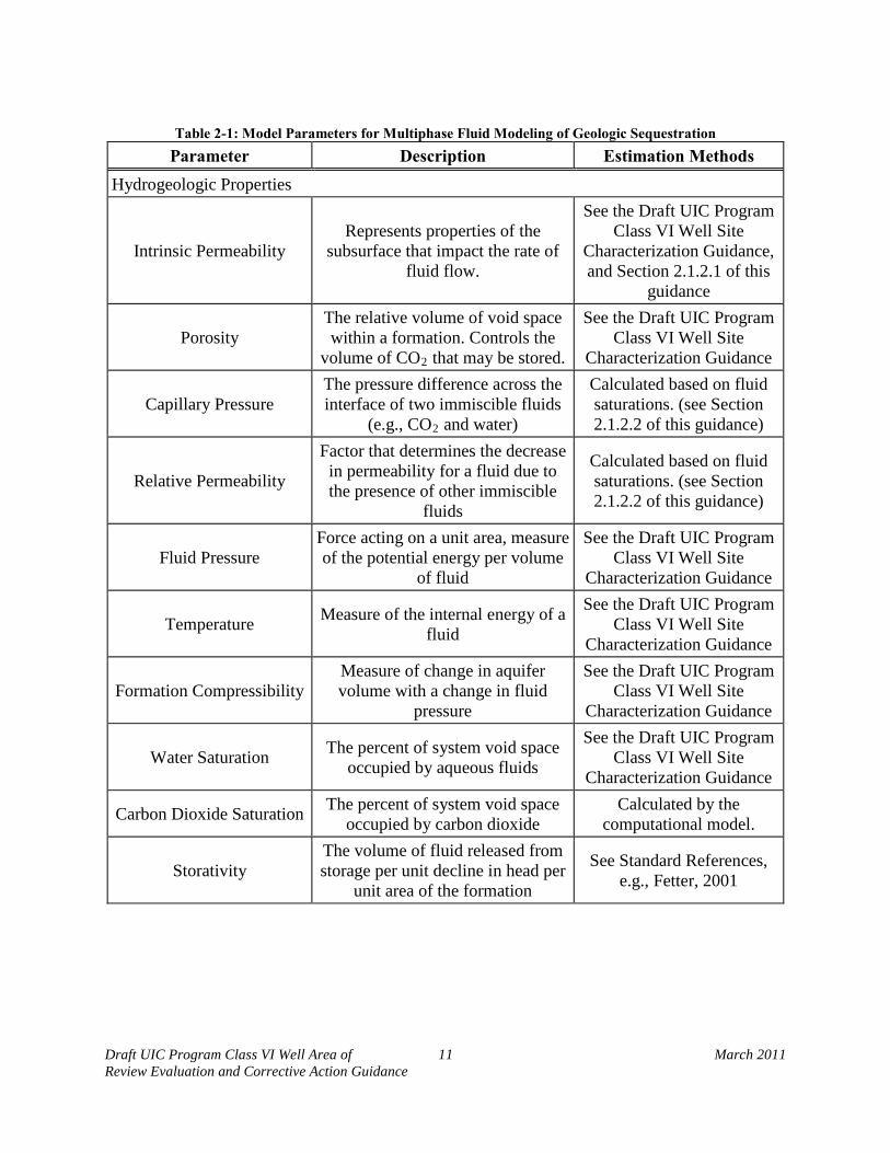
2.1.2. Model Parameters
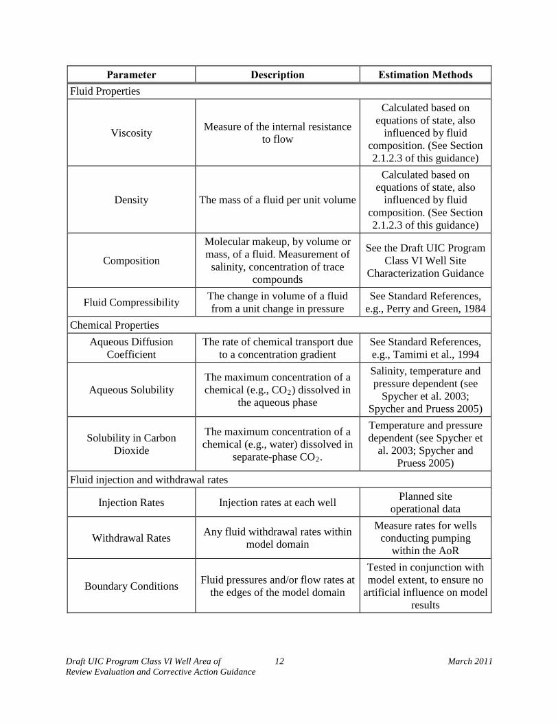
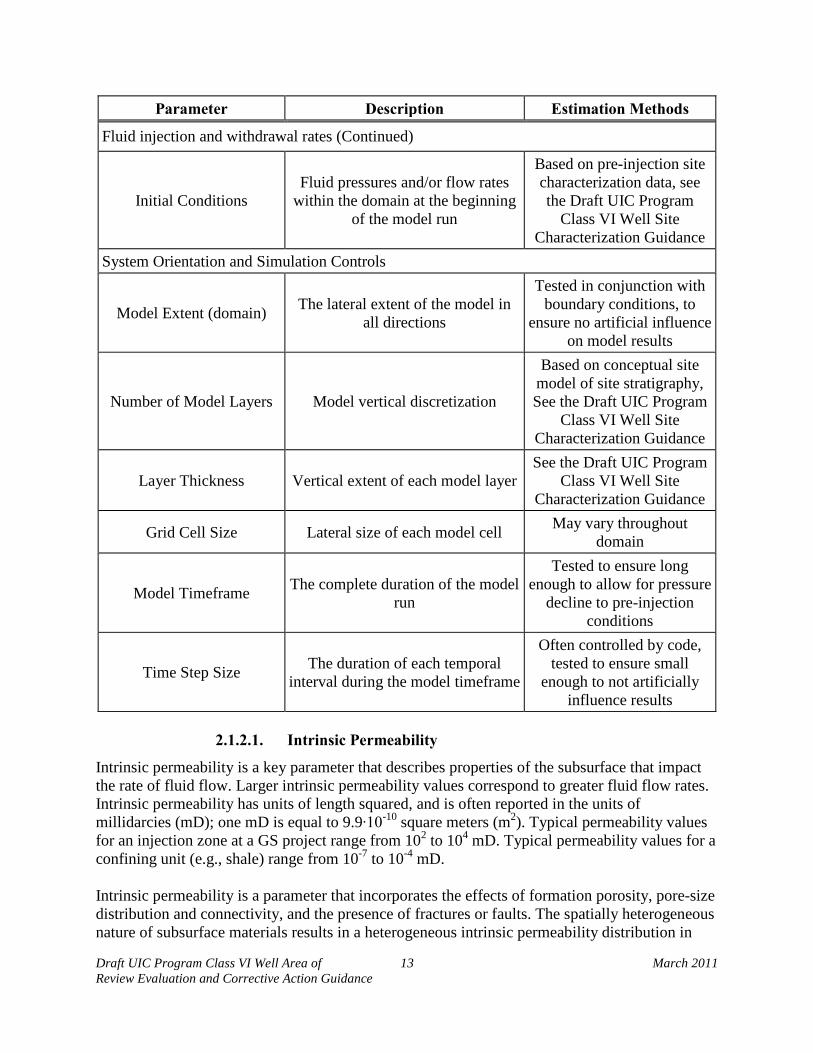
A parameter is a variable in the governing equations of the model that may be of uniform value throughout the domain, or may vary in space and time. While maintaining salient features of the hydrogeologic system, some system aspects are often lumped together in simulation models and described by effective parameters that are estimated or averaged from several data sources. Relevant parameters for multiphase flow modeling of GS are summarized in Table 2-1, and include hydrogeologic characteristics, fluid properties, chemical properties, fluid injection and withdrawal rates, initial and boundary conditions, system orientation (i.e., model domain, grid cell size), and simulation control parameters. Initial conditions describe parameter values at the start of the model run. Boundary condition parameters describe conditions of the system (e.g., fluid flow rates and/or pressures) at the edges of the model domain and at the location of injection and/or extraction wells.
Parameter values are to be based on site data to the extent possible. However, as discussed below, in cases where detailed site geologic characterization data are unavailable, parameter values may be estimated from standard values or relationships in the scientific literature. Model calibration, which may occur during AoR reevaluation, consists of adjusting a subset of the estimated parameter values to minimize the difference between model simulations and observed monitoring data. Model parameters may also be adjusted based on newly acquired site characterization data. For example, data gathered during well logging may inform updates to parameter values [§146.82 (c)(1)]. See the forthcoming Draft UIC Program Class VI Well Testing and Monitoring Guidance, when available, for more information. Particularly important parameters for GS include formation intrinsic permeability, porosity, relative permeability, and compressibility, and fluid viscosity and density.
Draft UIC Program Class VI Well Area of 11 March 2011 Review Evaluation and Corrective Action Guidance
Table 2-1: Model Parameters for Multiphase Fluid Modeling of Geologic Sequestration
Parameter Description Estimation Methods Hydrogeologic Properties
Intrinsic Permeability Represents properties of the
subsurface that impact the rate of fluid flow.
See the Draft UIC Program Class VI Well Site
Characterization Guidance, and Section 2.1.2.1 of this
guidance
Porosity The relative volume of void space within a formation. Controls the
volume of CO2 that may be stored.
See the Draft UIC Program Class VI Well Site
Characterization Guidance
Capillary Pressure The pressure difference across the interface of two immiscible fluids
(e.g., CO2 and water)
Calculated based on fluid saturations. (see Section 2.1.2.2 of this guidance)
Relative Permeability
Factor that determines the decrease in permeability for a fluid due to the presence of other immiscible
fluids
Calculated based on fluid saturations. (see Section 2.1.2.2 of this guidance)
Fluid Pressure Force acting on a unit area, measure of the potential energy per volume
of fluid
See the Draft UIC Program Class VI Well Site
Characterization Guidance
Temperature Measure of the internal energy of a fluid
See the Draft UIC Program Class VI Well Site
Characterization Guidance
Formation Compressibility Measure of change in aquifer volume with a change in fluid
pressure
See the Draft UIC Program Class VI Well Site
Characterization Guidance
Water Saturation The percent of system void space occupied by aqueous fluids
See the Draft UIC Program Class VI Well Site
Characterization Guidance
Carbon Dioxide Saturation The percent of system void space occupied by carbon dioxide
Calculated by the computational model.
Storativity The volume of fluid released from storage per unit decline in head per
unit area of the formation
See Standard References, e.g., Fetter, 2001
Draft UIC Program Class VI Well Area of 12 March 2011 Review Evaluation and Corrective Action Guidance
Parameter Description Estimation Methods Fluid Properties
Viscosity Measure of the internal resistance to flow
Calculated based on equations of state, also
influenced by fluid composition. (See Section 2.1.2.3 of this guidance)
Density The mass of a fluid per unit volume
Calculated based on equations of state, also
influenced by fluid composition. (See Section 2.1.2.3 of this guidance)
Composition
Molecular makeup, by volume or mass, of a fluid. Measurement of
salinity, concentration of trace compounds
See the Draft UIC Program Class VI Well Site
Characterization Guidance
Fluid Compressibility The change in volume of a fluid from a unit change in pressure
See Standard References, e.g., Perry and Green, 1984
Chemical Properties Aqueous Diffusion
Coefficient The rate of chemical transport due
to a concentration gradient See Standard References, e.g., Tamimi et al., 1994
Aqueous Solubility The maximum concentration of a chemical (e.g., CO2) dissolved in
the aqueous phase
Salinity, temperature and pressure dependent (see
Spycher et al. 2003; Spycher and Pruess 2005)
Solubility in Carbon Dioxide
The maximum concentration of a chemical (e.g., water) dissolved in
separate-phase CO2.
Temperature and pressure dependent (see Spycher et
al. 2003; Spycher and Pruess 2005)
Fluid injection and withdrawal rates
Injection Rates Injection rates at each well Planned site operational data
Withdrawal Rates Any fluid withdrawal rates within model domain
Measure rates for wells conducting pumping
within the AoR
Boundary Conditions Fluid pressures and/or flow rates at the edges of the model domain
Tested in conjunction with model extent, to ensure no
artificial influence on model results
Draft UIC Program Class VI Well Area of 13 March 2011 Review Evaluation and Corrective Action Guidance
Parameter Description Estimation Methods
Fluid injection and withdrawal rates (Continued)
Initial Conditions Fluid pressures and/or flow rates
within the domain at the beginning of the model run
Based on pre-injection site characterization data, see the Draft UIC Program
Class VI Well Site Characterization Guidance
System Orientation and Simulation Controls
Model Extent (domain) The lateral extent of the model in all directions
Tested in conjunction with boundary conditions, to
ensure no artificial influence on model results
Number of Model Layers Model vertical discretization
Based on conceptual site model of site stratigraphy, See the Draft UIC Program
Class VI Well Site Characterization Guidance
Layer Thickness Vertical extent of each model layer See the Draft UIC Program
Class VI Well Site Characterization Guidance
Grid Cell Size Lateral size of each model cell May vary throughout domain
Model Timeframe The complete duration of the model run
Tested to ensure long enough to allow for pressure
decline to pre-injection conditions
Time Step Size The duration of each temporal interval during the model timeframe
Often controlled by code, tested to ensure small
enough to not artificially influence results
2.1.2.1. Intrinsic Permeability
Intrinsic permeability is a key parameter that describes properties of the subsurface that impact the rate of fluid flow. Larger intrinsic permeability values correspond to greater fluid flow rates. Intrinsic permeability has units of length squared, and is often reported in the units of millidarcies (mD); one mD is equal to 9.9∙10-10 square meters (m2). Typical permeability values for an injection zone at a GS project range from 102 to 104 mD. Typical permeability values for a confining unit (e.g., shale) range from 10-7 to 10-4
mD.
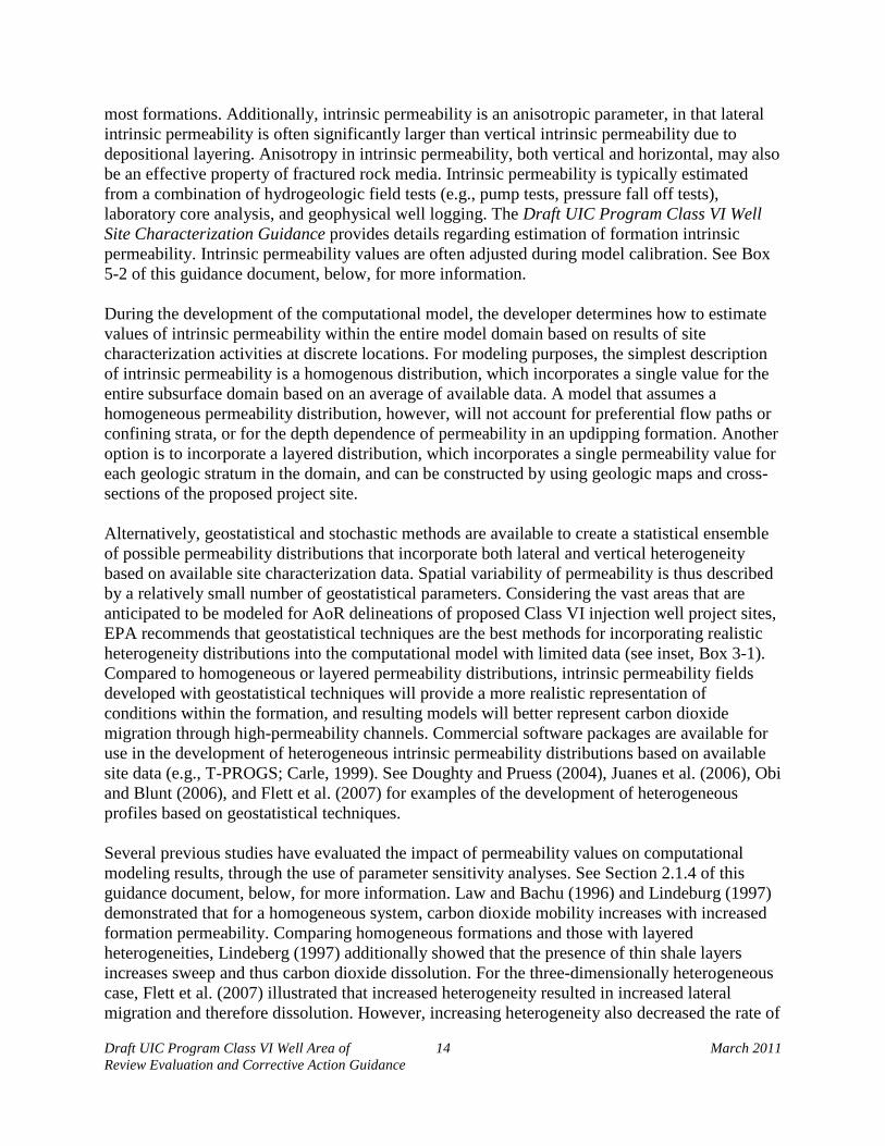
Intrinsic permeability is a parameter that incorporates the effects of formation porosity, pore-size distribution and connectivity, and the presence of fractures or faults. The spatially heterogeneous nature of subsurface materials results in a heterogeneous intrinsic permeability distribution in
Draft UIC Program Class VI Well Area of 14 March 2011 Review Evaluation and Corrective Action Guidance
most formations. Additionally, intrinsic permeability is an anisotropic parameter, in that lateral intrinsic permeability is often significantly larger than vertical intrinsic permeability due to depositional layering. Anisotropy in intrinsic permeability, both vertical and horizontal, may also be an effective property of fractured rock media. Intrinsic permeability is typically estimated from a combination of hydrogeologic field tests (e.g., pump tests, pressure fall off tests), laboratory core analysis, and geophysical well logging. The Draft UIC Program Class VI Well Site Characterization Guidance provides details regarding estimation of formation intrinsic permeability. Intrinsic permeability values are often adjusted during model calibration. See Box 5-2 of this guidance document, below, for more information.
During the development of the computational model, the developer determines how to estimate values of intrinsic permeability within the entire model domain based on results of site characterization activities at discrete locations. For modeling purposes, the simplest description of intrinsic permeability is a homogenous distribution, which incorporates a single value for the entire subsurface domain based on an average of available data. A model that assumes a homogeneous permeability distribution, however, will not account for preferential flow paths or confining strata, or for the depth dependence of permeability in an updipping formation. Another option is to incorporate a layered distribution, which incorporates a single permeability value for each geologic stratum in the domain, and can be constructed by using geologic maps and cross-sections of the proposed project site.
Alternatively, geostatistical and stochastic methods are available to create a statistical ensemble of possible permeability distributions that incorporate both lateral and vertical heterogeneity based on available site characterization data. Spatial variability of permeability is thus described by a relatively small number of geostatistical parameters. Considering the vast areas that are anticipated to be modeled for AoR delineations of proposed Class VI injection well project sites, EPA recommends that geostatistical techniques are the best methods for incorporating realistic heterogeneity distributions into the computational model with limited data (see inset, Box 3-1). Compared to homogeneous or layered permeability distributions, intrinsic permeability fields developed with geostatistical techniques will provide a more realistic representation of conditions within the formation, and resulting models will better represent carbon dioxide migration through high-permeability channels. Commercial software packages are available for use in the development of heterogeneous intrinsic permeability distributions based on available site data (e.g., T-PROGS; Carle, 1999). See Doughty and Pruess (2004), Juanes et al. (2006), Obi and Blunt (2006), and Flett et al. (2007) for examples of the development of heterogeneous profiles based on geostatistical techniques. Several previous studies have evaluated the impact of permeability values on computational modeling results, through the use of parameter sensitivity analyses. See Section 2.1.4 of this guidance document, below, for more information. Law and Bachu (1996) and Lindeburg (1997) demonstrated that for a homogeneous system, carbon dioxide mobility increases with increased formation permeability. Comparing homogeneous formations and those with layered heterogeneities, Lindeberg (1997) additionally showed that the presence of thin shale layers increases sweep and thus carbon dioxide dissolution. For the three-dimensionally heterogeneous case, Flett et al. (2007) illustrated that increased heterogeneity resulted in increased lateral migration and therefore dissolution. However, increasing heterogeneity also decreased the rate of
Draft UIC Program Class VI Well Area of 15 March 2011 Review Evaluation and Corrective Action Guidance
residual phase trapping by delaying water imbibition into previously carbon dioxide-filled pore space. Overall, increased heterogeneity resulted in slower carbon dioxide migration and decreased accumulation at the confining layer compared to a homogeneous case. Pruess (2008) showed that for discharge through a fault, decreased fault permeability resulted in delayed leakage to the surface and an increased maximum leakage rate.
Simulations by Zhou et al. (2008) indicate that patterns of formation pressure increase induced by carbon dioxide injection are sensitive to permeability. Larger formation permeability values resulted in less localized pressure increase surrounding the injection well. In addition, larger confining layer permeability resulted in less pressure buildup throughout the formation due to pressure dissipation and associated brine leakage.
2.1.2.2. Relative Permeability and Capillary Pressure
When immiscible fluids (e.g., carbon dioxide, water) are present within the pore spaces of a geologic formation, the ability for flow of one of those fluids is reduced, due to the blocking effect of the presence of the other fluid. This reduction in the capacity for fluid flow is represented by relative permeability, which is a factor, between 0 and 1, that is multiplied by the intrinsic permeability of a geologic formation in order to compute the effective permeability for a fluid in a particular pore space. The relative permeability of a fluid is based on the properties and amounts of all fluids present within the system. The greater the amount of pore space occupied by a particular fluid (measured as fluid saturation), the greater the relative permeability will be for that fluid. Because fluid saturations change over time and location, relative permeability values typically vary during model simulations.
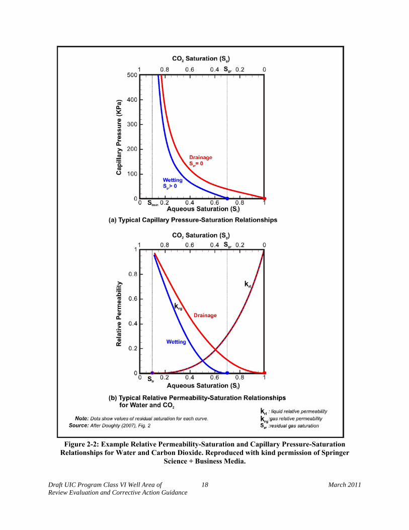
In order to simplify model calculations, the relative permeability for each fluid is calculated as a function of fluid saturations at each location and time within a model. This is achieved via a relative permeability-saturation function. The relative permeability-saturation function shape is based on properties of the porous media and fluids present at a particular site. Residual fluid saturation also impacts the shape of the relative permeability function, and describes the minimum fluid saturation within the porous medium following immiscible fluid displacement. An example relative permeability-saturation function is given in Figure 2-2. Note that this example function has been developed for a specific site (Doughty, 2007), and may not be applicable to other GS sites. Capillary pressure-saturation relationships (also known as characteristic curves) are also of importance because capillary pressure gradients provide the driving force for fluid movement under unsaturated conditions.
Previous research has shown that model predictions are very sensitive to the shape of the relative permeability-saturation functions used. The Draft UIC Program Class VI Well Site Characterization Guidance provides details regarding measurement of relative permeability. Ideally, laboratory core-analysis techniques will be used for experimental measurement of the relative permeability-saturation and capillary pressure-saturation functions for a particular site at reservoir conditions, with carbon dioxide and representative native fluids (e.g., Perrin et al., 2008; Bachu and Bennion, 2008; Plug and Bruining, 2007). If this is not feasible, relative permeability-saturation relationships may be estimated from core analysis using other immiscible fluids (e.g., Doughty et al., 2007). Alternatively, previously reported functions may be used, such
Draft UIC Program Class VI Well Area of 16 March 2011 Review Evaluation and Corrective Action Guidance
as those presented in Figure 2-2, if the experimental system was very similar to the site conditions for which the model will be applied. Relative permeability-saturation relationships are also commonly adjusted during model calibration. Relative permeability-saturation functional relationships and capillary pressure-saturation relationships (i.e., characteristic curves) can have a large impact on the predicted carbon dioxide mobility. Characteristic curves are described by a number of parameters, including residual carbon dioxide saturation. Doughty and Pruess (2004) compared site-specific characteristic curves to “generic” curves at the Frio, TX GS pilot project site and found that the choice of characteristic curves had a significant impact on plume size, shape and mobility. The authors point out that the differences in plume behavior for different sets of characteristic curves had important implications for operation and monitoring of the pilot test. Similarly, Doughty et al. (2007) found that model results were very sensitive to characteristic curve parameters. The authors constrained the value of characteristic curve parameters by calibration to monitoring data.
Pruess (2008) compared the effect of using three-phase characteristic curves developed for organic liquid-water-air systems (Stone, 1970) and simple linear characteristic curves. The choice of characteristic curves was found to have a very significant impact on the observed leakage rate of carbon dioxide through a fault system. The linear characteristic curves resulted in earlier leakage of carbon dioxide to the surface, and lower leakage rates. Use of three-phase relationships resulted in small fluid permeability at intermediate saturations due to phase-interference effects.
The impact of using hysteretic versus non-hysteretic characteristic curves has also been compared. Hysteresis refers to the dependence of the shape of the characteristic curve on the history of fluid flow within the formation. For example, characteristic curves are often observed to have a different shape when non-wetting fluids (e.g., supercritical carbon dioxide) are displacing wetting fluids (e.g., formation water), than when wetting fluids are displacing non-wetting fluids. Juanes et al. (2006) showed that consideration of hysteresis and capillary trapping resulted in a more spread out carbon dioxide distribution with less accumulation at the confining layer. Doughty (2007) found that results from simulations with non-hysteretic curves did a poor job of matching hysteretic curves in homogeneous and heterogeneous media. Relative to non-hysteretic cases, hysteresis caused a more mobile plume leading edge (where there is no water imbibition), and a slower trailing edge with a significant amount of residual trapping (due to water imbibition).
2.1.2.3. Injection Rate
The carbon dioxide injection rate at proposed Class VI injection wells is incorporated into the model by assigning the injection rate parameter at a constant or variable-rate boundary condition. Several researchers have reported that increasing the carbon dioxide injection rate results in increased migration rates (e.g., Law and Bachu, 1996; Saripalli and McGrail, 2002; Juanes et al., 2006). Juanes et al. (2006) considered capillary trapping in highly heterogeneous media, and found that increased injection rate resulted in more residual trapping due to invasion of carbon dioxide into a wider range of pore sizes. Therefore, in the long term, increased injection rates
Draft UIC Program Class VI Well Area of 17 March 2011 Review Evaluation and Corrective Action Guidance
actually decreased the final extent of carbon dioxide migration, as more mass was immobilized through capillary forces. Pruess (2008) modeled leakage to the ground surface through a fault system, and found that larger injection rates resulted in increased enhancement of maximum surface discharge rates relative to injection rates.
2.1.2.4. Mineral Precipitation Kinetic Parameters
Mineral precipitation is a subset of reactive transport problems and represents a trapping mechanism for carbon dioxide as well as a mechanism for permeability modification. As discussed above in Section 2.1.1, the GS rule does not stipulate that reactive transport be considered in AoR delineation modeling. However, the owner or operator, or UIC Program Director, may determine that reactive transport modeling be considered for a particular project.
Studies accounting for mineral precipitation typically include precipitation kinetic (i.e., rate) parameters. Although precipitation rates have a large impact on mineral trapping, there is a great deal of uncertainty related to these parameters (Knauss et al., 2005; Xu et al., 2006). Furthermore, complex interrelationships exist between the rates of separate mineral species in a formation. For example, a sensitivity analysis for trapping through dawsonite [NaAl(CO3)(OH)2] precipitation showed that decreasing dawsonite kinetics resulted in increased formation of other trapping minerals calcite [CaCO3] and magnesite [MgCO3]
(Knauss et al., 2005). Izgec et al. (2008) showed that changes in formation permeability resulting from mineralization reactions were very sensitive to kinetic rate parameters.
Draft UIC Program Class VI Well Area of 18 March 2011 Review Evaluation and Corrective Action Guidance
Figure 2-2: Example Relative Permeability-Saturation and Capillary Pressure-Saturation Relationships for Water and Carbon Dioxide. Reproduced with kind permission of Springer
Science + Business Media.
Draft UIC Program Class VI Well Area of 19 March 2011 Review Evaluation and Corrective Action Guidance
2.1.2.5. Fluid Properties and Equations of State
The density, viscosity, and phase-state of the carbon dioxide injectate, ground water, and any other fluids that may be present (e.g., hydrocarbons), are important model input parameters. However, these properties change significantly across the temperature and pressure range that will be encountered at GS projects. The equations of state describe these fluid properties as a function of pressure and temperature, and are used by the model to calculate properties at conditions encountered in the simulation as they change with location and time. Graphs developed from accepted equations of state for carbon dioxide are depicted in Figure 2-1. Previous studies have shown that model results are sensitive to the equations of state used (Pruess et al., 2004; Han and McPherson, 2008).
The composition of the injectate will be reflected in several chemical and physical parameters assigned to the carbon dioxide fluid in the model simulations. Several studies have evaluated the impact of common carbon dioxide stream contaminants H2S and SO2
on geochemical reactions and mineral trapping. Both Knauss et al. (2005) and Xu et al. (2007) showed that the addition of hydrogen sulfide had little impact, whereas the addition of sulfur dioxide resulted in a lower pH in the injection zone, less carbon-bearing mineral precipitation, and more formation-mineral dissolution.
2.1.2.6. Mass-Transfer Coefficients
Mass transfer coefficients describe the equilibrium concentration of chemical constituents (e.g., water, carbon dioxide) between separate phases. For example, the equilibrium aqueous concentration of carbon dioxide dissolved in ground water in contact with separate-phase (e.g., supercritical) carbon dioxide is described by a partitioning coefficient. Other mass-transfer coefficients describe the distribution of constituents between the gaseous, aqueous, separate-phase carbon dioxide, and solid phases. For the case of reactive transport modeling, mass-transfer coefficients describe equilibrium concentration of constituents between mineral and dissolved phases. Similar to fluid properties, mass-transfer coefficients are in many cases temperature and pressure dependent. Mass-transfer coefficients may also be dependent on properties of the formation and fluids present, such as ground water salinity. Reference documents are available that provide many necessary mass-transfer coefficients (e.g., Green and Perry, 2008), and several commonly used codes include necessary mass-transfer coefficients (e.g., TOUGH2-ECO2N; Pruess and Spycher, 2007).
2.1.2.7. Model Orientation and Gridding Parameters
Numerical modeling requires the developer to define the spatial and temporal domains, grid spacing and gridding routine, and domain boundary conditions. These features of the model are typically designed with an effort to minimize computational demand and therefore processing time. However, there is potential for erroneous results based on numerical features of the model (i.e., numerical artifacts), which can mask or enhance the effects of physical processes. A few studies have focused on evaluating the impacts of numerical artifacts for models of GS.
Draft UIC Program Class VI Well Area of 20 March 2011 Review Evaluation and Corrective Action Guidance
Doughty and Pruess (2004) tested the impact of varying grid block sizes for a model of the Frio formation pilot GS project site in Texas. They found that the overall pattern of plume movement was similar for different grid sizes, but overly coarse grids were not able to simulate buoyancy-driven flow within individual sand channels. The authors also observed that the choice of grid block sizes and gridding routine could result in preferential flow in the grid axis direction and numerical dispersion. Similarly, Juanes et al. (2006) observed that overly coarse grid block sizes that did not capture specific migration pathways overestimated carbon dioxide movement and the amount of capillary trapping. Doughty et al. (2007) note that higher-resolution models are needed for understanding of near well-bore effects. As noted in Section 2.1.3.1 of this guidance document, below, methods have been developed to establish numerical grids with high resolution in areas of interest (e.g., near well-bores), and lower resolution in other areas, such as near the model area boundaries.
2.1.3. Computational Approaches
Computational codes consist of the set of interrelated mathematical equations (i.e., governing equations, constitutive relationships, and equations of state) that are solved simultaneously in order to predict fluid movement, pressure changes, and other changes, as a function of both location and time. These equations include complex partial differential equations that cannot be easily solved, and require complex estimation techniques. For the most part, numerical estimation approaches, discussed below, will be necessary in order to adequately represent the several physical processes necessary to delineate the AoR and successfully comply with GS Rule in preparing a Class VI injection well permit application.
In certain circumstances, simpler analytic and semi-analytic approaches may be used to complement numerical efforts in delineating the AoR. As discussed below, analytic and semi-analytic approaches are not capable of representing several processes and features that are important for predictions of fluid movement, and often assume simple geometry and homogeneity.
2.1.3.1. Numerical Approaches
Computational models used for practical applications typically consist of a numerical formulation of the governing equations applied over a spatially discretized model domain that defines the spatial extent and resolution of the problem (i.e., the model grid). This formulation is solved by a numerical method, such as finite element or finite difference approximation. The model grid is partitioned into grid cells, smaller spatial sub-units within the model grid. Fluid and heat flow is then solved between adjoining grid cells, while maintaining a mass balance within the model. Phase changes, mass transfer, and chemical reactions can also be calculated for phases and constituents within a cell. Each cell can be assigned unique parameter values for physical properties (i.e., intrinsic permeability, porosity), allowing for three-dimensional, detailed representations of physical heterogeneity. Numerical models may be used for steady-state problems (in which injection and withdrawal rates are constant and the solution is obtained only for infinite time) and transient problems (in which injection and withdrawal rates may vary in time, and the solution is obtained at several discrete times during the model timeframe).
Draft UIC Program Class VI Well Area of 21 March 2011 Review Evaluation and Corrective Action Guidance
In addition to detailed geologic heterogeneity, numerical models are typically capable of representing density-driven fluid flow (e.g., the buoyancy of carbon dioxide), and the dissolution of carbon dioxide into ground water. Numerical models can also represent irreducible fluid saturations (i.e., the amount of fluid being ‘trapped’ in geologic formation pore space even after another immiscible fluid has passed through that area), multiphase flow effects, and the concomitant reduced permeability.
The scale of spatial and temporal discretization of the model affects the accuracy of the solutions to these numerical formulations. Finer scales of time and space reduce numerical solution error. However, computational demand increases as the length scale (e.g., grid cell size) and time scale (e.g., time-step size) decrease, and as additional processes are simulated. Methods have been developed to mitigate increases in computational demand, while focusing on regions and times of interest, such as adaptive grid block size (i.e., mesh) refinement. Another possibility is the use of parallel computing, in which a single problem is broken up and distributed among many processors (e.g., Zhang et al., 2007).
2.1.3.2. Analytical, Semi-analytical, and Hybrid Approaches
Analytical and semi-analytical models may be used to complement numerical modeling efforts in AoR delineation for Class VI wells. Compared to numerical models, analytical models have much lower computational requirements and therefore processing times. Analytical and semi-analytical codes may also be particularly useful for assessing the transport of carbon dioxide through abandoned wellbores, which is difficult in numerical models due to the disparity in spatial scales. Analytical and semi-analytical models also may be used as screening tools to quickly assess potential storage sites, or as a relatively simple comparative check on numerical modeling results. Celia and Nordbotten (2009) suggest the use of hybrid numerical-analytical models for cases where a large-scale numerical model could be combined with local analytical models (e.g., describing wells), or the use of semi-analytical solutions where analytical solution is used in the spatial dimension and finite-stepping is used for temporal changes.
However, strictly analytical and semi-analytical models are not able to explicitly simulate capillary trapping, varying injection rates, or account for formation heterogeneity. The applicability of these models is limited to simplified cases where an exact function can be found to satisfy the governing equation, and boundary and initial conditions. For example, these models assume homogenous aquifers (i.e., no variability in physical structure, porosity, or intrinsic permeability). For most formations this is an unrealistic assumption, and neglects preferential fluid movement through heterogeneous channels within geologic formations. Therefore, EPA recommends that analytic and semi-analytic models not be used as the sole basis for AoR delineation.
2.1.4. Model Uncertainty and Sensitivity Analyses
As discussed above, computational models are an approximate representation of reality, and thus predictions exhibit some degree of uncertainty. Model uncertainty is a result of the uncertainties related to the underlying science of the governing equations and the uncertainty in the parameter values input to represent the actual system (US EPA, 2003). Uncertainty in governing equations
Draft UIC Program Class VI Well Area of 22 March 2011 Review Evaluation and Corrective Action Guidance
and model framework may arise from incomplete scientific data or lack of knowledge, and the necessary simplifications that translate scientific concepts into mathematical equations. Parameter uncertainty results from poor data quality (e.g., measurement errors, analytical imprecision, limited sample size), lack of data, and the inherent data variability in natural systems. Model predictions depend largely on the values input for a number of key parameters and thus may be significantly impacted by incomplete knowledge, or they may be process and scale dependant. A model’s predictive accuracy improves with improved data quality and quantity.
Significant uncertainty exists in modeling predictions of GS due to the difficulty in determining the geological formation structure and permeability field throughout the extensive area likely to be impacted by proposed large injection volumes, a relative lack of data on the behavior of supercritical carbon dioxide in the subsurface, the drastic changes in transport behavior of carbon dioxide caused by changes in pressure and/or temperature, and the buoyant nature of carbon dioxide relative to native formation ground water. The predictive accuracy of a model will improve as the model is calibrated over time, minimizing the differences between observed and simulated data.
The impact of parameter uncertainty on modeling results can be characterized through a model sensitivity analysis, which consists of sequentially varying a single parameter in successive model simulations while keeping all other model features constant. Sensitivity analyses provide an indication of those modeling parameters that most impact predictions of carbon dioxide migration, trapping, and pressure changes, and provide guidance for what parameters to focus on during data collection, parameter estimation, and model calibration. EPA recommends that owners or operators include sensitivity analyses in submission of modeling results when communicating predictions, consistent with previous guidance on environmental modeling (e.g., NRC, 2007).
2.2. Existing Codes used for Development of GS Models
A wide variety of modeling exercises have been reported in the peer reviewed literature for GS, and have been reviewed previously (Schnaar and Digiulio, 2009). Several computational codes have been developed for multiphase flow and transport problems, and a number of these codes are publicly or commercially available for the owner(s) or operator(s) of a GS project to use in AoR delineation modeling. Codes reported in the literature used for modeling of GS include petroleum reservoir codes (STARS, Law and Bachu, 1996; ECLIPSE, Zhou et al., 2004; Juanes et al., 2006; CHEARS, Flett et al., 2007) and codes that have been developed at U.S. Department of Energy (DOE) national labs for a range of multiphase flow and transport problems (CRUNCH, Knauss et al., 2005; TOUGH-series, Finsterle, 2004; Xu et al., 2006; Doughty and Pruess, 2004; Doughty, 2007). These codes vary not only in the physical processes considered, but also in numerical techniques such as the spatial discretization method, iteration approach, and gridding routines.
Codes used for modeling GS consider multiphase flow of carbon dioxide in supercritical, liquid, and gaseous phases including miscible and immiscible displacement, dissolution of carbon dioxide in ground water, density-driven flow, and flow of ground water as impacted by injection.
Draft UIC Program Class VI Well Area of 23 March 2011 Review Evaluation and Corrective Action Guidance
Available codes may also be further categorized based on their ability to consider, or be adjusted to consider, complex three-dimensionally heterogeneous formations, residual phase trapping and characteristic-curve hysteresis, mineral precipitation/dissolution reactions and subsequent mineral phase trapping and leaching of heavy metals, carbon dioxide sorption in coal-bed methane problems, and leakage through abandoned wellbores. Models based on the TOUGH-series codes have been widely reported in the literature, and are capable of considering three-dimensional heterogeneous formations, carbon dioxide dissolution, residual phase trapping and characteristic-curve hysteresis, coupled fluid flow and geomechanical processes, and mineral precipitation (e.g., Finsterle, 2004; Doughty, 2007; Xu et al., 2006; Rutqvist et al., 2008).
Several codes were compared for common GS problems in a Lawrence Berkeley National Laboratory (LBNL) study (Pruess et al., 2004). Ten research groups representing six countries participated in the study. The codes evaluated included TOUGH-series codes (LBNL, CSIRO Petroleum, Industrial Research Limited), ECLIPSE 300 (Los Alamos National Laboratory), and STOMP (Pacific Northwest National Laboratory), among others. The problems considered varied in complexity and included mixture of gases in an open system, radial flow from an injection well, discharge along a fault zone, injection with mineral trapping, and injection with enhanced-oil recovery. For the most part, model results for the different codes were found to be in good agreement. Most discrepancies were traced to differences in the calculation of fluid properties (e.g., viscosity). These results emphasize the need for accurate descriptors of carbon dioxide transport properties and equations of state.
The use of proprietary codes (i.e., not available for free to the general public) may prevent full evaluation of model results (e.g., NRC, 2007). There are several aspects of a model that can be proprietary, and some may be more problematic than others for computational model evaluation. For example, use of a proprietary user-interface with a publicly available code may not present a significant problem. Several popular codes in the petroleum-reservoir engineering discipline are proprietary (e.g., ECLIPSE). However, operators of particular GS sites may prefer to use these codes as they have previous experience with them, and they have been used in peer-reviewed studies to model GS. As discussed below, when using a proprietary model for AoR delineation, site operators of GS projects are encouraged to clearly disclose to the UIC Program Director the code assumptions, and if necessary, governing equations and equations of state with the permit application.
Draft UIC Program Class VI Well Area of 24 March 2011 Review Evaluation and Corrective Action Guidance
3. AoR Delineation Using Computational Models
Determination of the AoR for proposed Class VI wells will consist of data collection and compilation, development of the site computational model, delineation of the AoR based on model results, and submitting of the model results and AoR delineation to the UIC Program Director with the Class VI injection well permit application. The AoR and Corrective Action Plan must describe how the owner or operator plans to conduct these activities and is subject to Program Director approval [§146.84 (b)]. See the Draft UIC Program Class VI Well Project Plan Development Guidance for more information on the AoR and Corrective Action Plan. This section below describes each of the remaining steps in AoR delineation, and provides several quantitative examples revolving around a hypothetical GS site. EPA recommends that model development in all cases be conducted by a professional expert with the understanding of multiphase flow processes and experience with application of sophisticated computational models.
3.1. Data Collection and Compilation
Computational modeling organizes the required collected site characterization data for a proposed Class VI injection well site and applies scientifically accepted principles to estimate the carbon dioxide plume and pressure front migration. The extent to which site and operational conditions are realistically represented determines the validity of the resulting model predictions. Site characterization data inform model parameterization, and therefore, adequate data collection, analysis and compilation are integral components of model development. Table 2-1 of this guidance provides a summary of important model parameters, many of which are determined based on site characterization data.
Extensive site characterization data are required to be collected for proposed GS projects [§§146.82 and 146.83]. These data are required to verify that the proposed injection zone at the characterized site has adequate injectivity to accept the injected carbon dioxide at the proposed rate, and adequate volume to store the injectate over the lifetime of the project. Furthermore, site characterization data verify that suitable confining zone(s) are present to restrict the upwards movement of carbon dioxide. Additional features of the site, such as baseline geochemistry and pre-injection fluid pressures, inform the interpretation of future monitoring results. As discussed below, much of the site characterization data collected at the proposed Class VI injection well site are also necessary in order to inform computational model development and AoR delineation. Site characterization requirements and methods are discussed in more detail in the Draft UIC Program Class VI Well Site Characterization Guidance.
3.1.1. Site Hydrogeology
Regional and site-specific geology provide the foundations of the computational model used to delineate the AoR. This includes site stratigraphy, including formation elevation and thickness, as presented in cross sections and/or topographic maps. Any data regarding structural geology, including folding, and fracture and fault systems are recommended to also be identified and used in creating the computational model. Hydrogeologic information, including initial fluid pressure and head, horizontal and vertical gradients, and ground water flow direction and velocity, are
Draft UIC Program Class VI Well Area of 25 March 2011 Review Evaluation and Corrective Action Guidance
important considerations for each geologic formation at the proposed injection site. This information is often presented in the form of maps and cross sections. Other important characteristics include intrinsic permeability and porosity of all formations ranging from the uppermost USDW to beneath the injection zone. EPA recommends that the heterogeneity of these characteristics within each formation also be evaluated. Data regarding the heterogeneity of these parameters are of particular importance in representing the injection and confining zone(s). The GS Rule requires that AoR computational modeling take into account any geologic heterogeneities and other discontinuities [§146.84 (c)(1)(ii)].
Thorough characterization of multiphase flow parameters is also recommended in order to properly inform the computational modeling. These include parameters describing the capillary pressure-saturation and relative permeability-saturation relationships of each formation, with the injection and confining zones being of particular importance. See Figure 2-2 of this guidance for more information. EPA recommends that accepted formulations of these relationships be defined that are as specific to the site and fluids of interest (e.g., brine, carbon dioxide) as possible, as discussed above in Section 2.1.2.2 of this guidance.
The quantity of data used to inform model development may be based on the GS Rule site characterization requirements, as discussed in the Draft UIC Program Class VI Well Site Characterization Guidance. For pertinent data types, as discussed above, all data collected to comply with site characterization requirements may be considered in the AoR delineation. Furthermore, EPA recommends that any additional pertinent data available in the vicinity of the site, for example from U.S. Geological Survey (USGS) or other studies, also be included in model development. Additionally, EPA recommends that the lateral and vertical extents of all formations predicted to exhibit contact with supercritical carbon dioxide or elevated pressure over the lifetime of the proposed GS project be well characterized. This may be an iterative process because initial model estimates of plume and pressure front migration may indicate further migration than previously assumed. In these cases, some additional site characterization in these regions may be requested by the UIC Program Director before a permit is approved.
EPA recommends that adequate data be collected to reasonably estimate site heterogeneity. Collection of sufficient data is always a challenge in geologic studies, and this is compounded by the large areas that may be impacted by GS projects. Use of geophysical site characterization techniques may reduce the burden of site characterization over large areas. See the Draft UIC Program Class VI Well Site Characterization Guidance for more information on using geophysical methods to assist with collecting the required site characterization data for a Class VI injection well permit application.
3.1.2. Operational Data
The GS Rule requires that the AoR computational modeling for a Class VI injection well be based on existing operational data, including injection pressures, rates, and total volumes over the lifetime of the GS project [§146.84(c)(1)(i)]. EPA recommends that operational data also include the location, and number of injection wells, and the injection well construction details
Draft UIC Program Class VI Well Area of 26 March 2011 Review Evaluation and Corrective Action Guidance
(e.g., total depth, perforated interval). In the case of GS projects with multiple Class VI injection wells, it is important to note that each Class VI well is required to be permitted separately, as area permits are not allowed [§144.33(a)(5)]. However, EPA strongly encourages potential Class VI injection well owners and operators to account for all injection wells associated with the proposed project, or any other injection or extraction wells in the area, in the AoR model development. If allowed by the UIC Program Director, a single AoR delineation model can be used for all Class VI injection well wells for a single GS project, as long as the model includes the influences of all relevant wells. EPA also recommends that overlapping pressure perturbations be evaluated for a given basin to determine any combined risk to USDWs. The owner or operator may consult the UIC Program Director regarding any existing or planned projects in the vicinity of the proposed well.
3.2. Model Development
Once adequate data are collected, model development consists of the formation of a conceptual site model, design of the mathematical framework and grid, and parameterization (i.e., determination of input parameter values) (US EPA, 2003). The model is then executed to provide predictions of fluid movement and pressure perturbations during the lifetime of the project.
3.2.1. Conceptual Model of the Proposed Injection Site
A conceptual site model is a schematic representation of the GS project that will be modeled, including any relevant physical processes. The conceptual site model is informed primarily by the collected site characterization data and the proposed operational conditions, such as well-field configuration and injection rates. EPA recommends that descriptions of the conceptual site model present a clear statement and description of each element of the site, any assumptions and hypotheses related to the proposed injection site, as well as the reasoning behind them (e.g., lab experiments, empirical data, or peer-reviewed literature). The conceptual site model also identifies the modeling region in three dimensions. Geologic stratigraphy, any other relevant geologic features, all physical processes that will impact migration of carbon dioxide and ground water, chemical species of interest, location of USDWs and potential conduits, conditions at site boundaries that may inform model boundary conditions, and areas of sparse site characterization data are also identified in the conceptual site model. See Box 3-1 of this guidance document, below, for more information about the conceptual site model.
3.2.2. Determination of Physical Processes to be Included in the Computational
Model
Prior to developing the computational model for a proposed Class VI injection well AoR delineation, the owner(s) or operators(s) will need to determine what physical processes will be considered in the computational model. This determination is based on the most significant processes identified in the conceptual model, as well as those processes that can be realistically included in the computational model. At a minimum, the GS Rule requires that the model include multiphase flow of carbon dioxide and formation fluids [§146.84(c)(1)]. Additional processes may be required for certain projects. For example, reactive transport could be relevant if permeability and/or porosity are predicted to change as a result of precipitation/dissolution
Draft UIC Program Class VI Well Area of 27 March 2011 Review Evaluation and Corrective Action Guidance
reactions. Geomechanical processes could be relevant if pressure and stress may change hydrogeologic properties. If the aqueous carbon dioxide plume is a potential risk factor, the carbon dioxide dissolution into ground water may also be considered in the AoR delineation model.
However, including reactive transport and geomechanical processes may be impractical for some applications of the model due to the large increases in computational demands (i.e., extremely long computer processing times), lack of meaningful data on mineral precipitation/dissolution kinetics, and the inability of the preferred computational code to include these processes. Furthermore, including these processes may be unnecessary in many cases because the impact on plume and pressure front migration may be relatively minor. The GS Rule does not require including reactive transport and geomechanical processes in the AoR delineation modeling. However, the UIC Program Director may request that the owner(s) or operator(s) include these additional processes in AoR delineation modeling information submitted with the proposed the AoR delineation model for a proposed Class VI injection well.
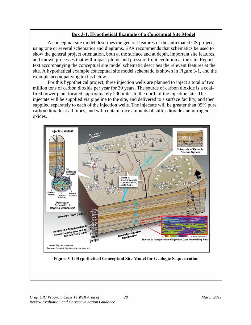
Draft UIC Program Class VI Well Area of 28 March 2011 Review Evaluation and Corrective Action Guidance
Box 3-1. Hypothetical Example of a Conceptual Site Model
A conceptual site model describes the general features of the anticipated GS project, using one or several schematics and diagrams. EPA recommends that schematics be used to show the general project orientation, both at the surface and at depth, important site features, and known processes that will impact plume and pressure front evolution at the site. Report text accompanying the conceptual site model schematic describes the relevant features at the site. A hypothetical example conceptual site model schematic is shown in Figure 3-1, and the example accompanying text is below.
For this hypothetical project, three injection wells are planned to inject a total of two million tons of carbon dioxide per year for 30 years. The source of carbon dioxide is a coal-fired power plant located approximately 200 miles to the north of the injection site. The injectate will be supplied via pipeline to the site, and delivered to a surface facility, and then supplied separately to each of the injection wells. The injectate will be greater than 99% pure carbon dioxide at all times, and will contain trace amounts of sulfur dioxide and nitrogen oxides.
Figure 3-1: Hypothetical Conceptual Site Model for Geologic Sequestration
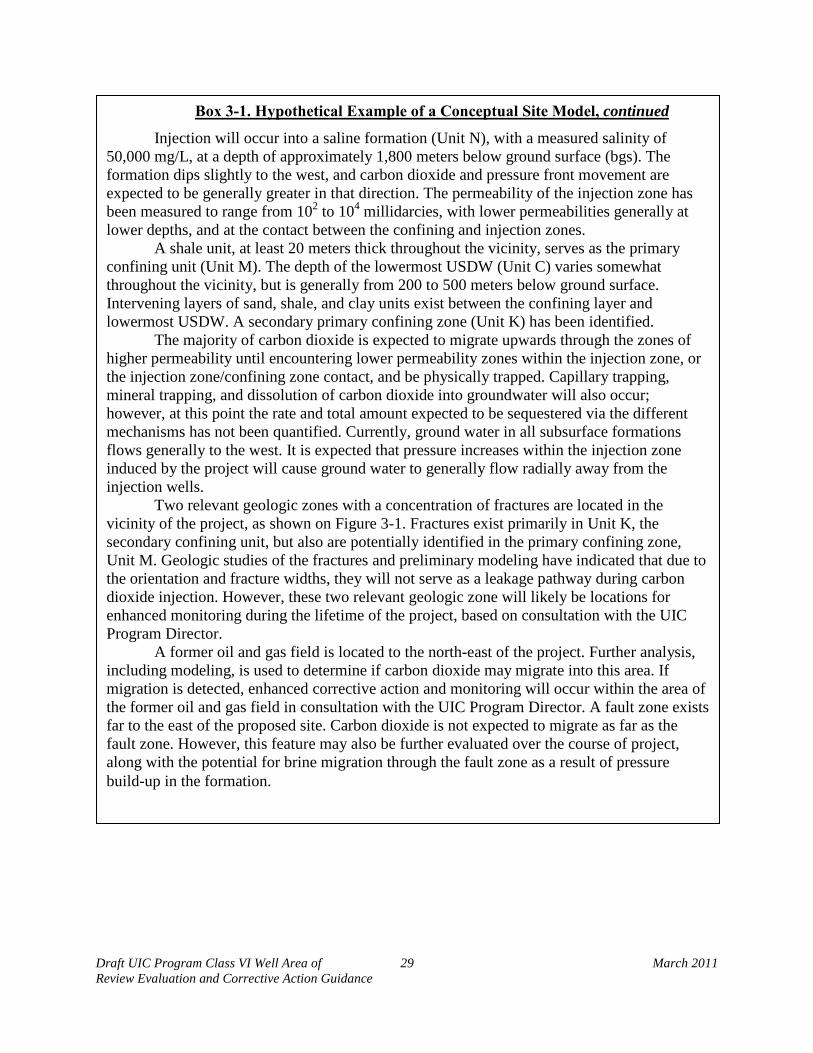
Draft UIC Program Class VI Well Area of 29 March 2011 Review Evaluation and Corrective Action Guidance
Box 3-1. Hypothetical Example of a Conceptual Site Model, continued
Injection will occur into a saline formation (Unit N), with a measured salinity of 50,000 mg/L, at a depth of approximately 1,800 meters below ground surface (bgs). The formation dips slightly to the west, and carbon dioxide and pressure front movement are expected to be generally greater in that direction. The permeability of the injection zone has been measured to range from 102 to 104 millidarcies, with lower permeabilities generally at lower depths, and at the contact between the confining and injection zones.
A shale unit, at least 20 meters thick throughout the vicinity, serves as the primary confining unit (Unit M). The depth of the lowermost USDW (Unit C) varies somewhat throughout the vicinity, but is generally from 200 to 500 meters below ground surface. Intervening layers of sand, shale, and clay units exist between the confining layer and lowermost USDW. A secondary primary confining zone (Unit K) has been identified.
The majority of carbon dioxide is expected to migrate upwards through the zones of higher permeability until encountering lower permeability zones within the injection zone, or the injection zone/confining zone contact, and be physically trapped. Capillary trapping, mineral trapping, and dissolution of carbon dioxide into groundwater will also occur; however, at this point the rate and total amount expected to be sequestered via the different mechanisms has not been quantified. Currently, ground water in all subsurface formations flows generally to the west. It is expected that pressure increases within the injection zone induced by the project will cause ground water to generally flow radially away from the injection wells.
Two relevant geologic zones with a concentration of fractures are located in the vicinity of the project, as shown on Figure 3-1. Fractures exist primarily in Unit K, the secondary confining unit, but also are potentially identified in the primary confining zone, Unit M. Geologic studies of the fractures and preliminary modeling have indicated that due to the orientation and fracture widths, they will not serve as a leakage pathway during carbon dioxide injection. However, these two relevant geologic zone will likely be locations for enhanced monitoring during the lifetime of the project, based on consultation with the UIC Program Director.
A former oil and gas field is located to the north-east of the project. Further analysis, including modeling, is used to determine if carbon dioxide may migrate into this area. If migration is detected, enhanced corrective action and monitoring will occur within the area of the former oil and gas field in consultation with the UIC Program Director. A fault zone exists far to the east of the proposed site. Carbon dioxide is not expected to migrate as far as the fault zone. However, this feature may also be further evaluated over the course of project, along with the potential for brine migration through the fault zone as a result of pressure build-up in the formation.
Draft UIC Program Class VI Well Area of 30 March 2011 Review Evaluation and Corrective Action Guidance
3.2.3. Computational Model Design
After a conceptual site model has been developed, and the processes that will be considered have been determined, the next step is to develop the site computational model. This includes the determination of an appropriate computational code, and parameterization (i.e., populating the code with the selected site-specific parameters) in order to develop the model.
3.2.3.1. Computational Code Determination
In order to create the computational model, EPA recommends that a code be used that includes routines for the relevant physical processes at the site based on peer-reviewed theory and equations, including equations-of-state for carbon dioxide and other chemical species of interest, as discussed above in Section 2.1.2.3 of this guidance document. EPA recommends that the code also include accurate mass-transfer coefficients, including solubility of carbon dioxide, as a function of primary thermodynamic variables (i.e., temperature, pressure, phase saturations). If using an independently developed or untested code, EPA also recommends that the developer model test cases found in the literature in order to verify model accuracy before submitting the Class VI injection well permit application to the UIC Program Director (e.g., see Pruess et al., 2004).
3.2.3.2. Model Spatial Extent, Discretization, and Boundary
Conditions
The computational model will be designed by determining the spatial boundaries of the problem and spatial discretization. It is recommended that lateral grid spacing be fine enough to resolve heterogeneities, as discussed above (e.g., Doughty and Pruess, 2004). Vertically, the model is recommended to include the injection zone, all overlying zones, and any USDWs. Boundary conditions are typically based on hydrogeologic conditions in locations corresponding to the edges of the model domain. Model testing may be conducted to ensure that grid spacing, gridding routine, and boundary conditions do not result in numerical artifacts that impact the model results. If results of such testing indicate artificial impacts, then adjustment of the model may be necessary prior to running the model for a proposed Class VI injection well AoR delineation.
3.2.3.3. Model Timeframe
The GS Rule requires that the model used to delineate the AoR for a proposed Class VI injection well be run from the commencement of injection activities until the plume movement ceases, until pressure differentials sufficient to cause the movement of injected fluids or formation fluids into a USDW are no longer present, or until the end of a fixed time period as determined by the UIC Program Director [§146.84(c)(1)]. EPA recommends that in all cases, the model is run long enough after injection operations cease that the migration of the carbon dioxide plume and pressure front have ceased to migrate, and steady-state conditions are reached in the subsurface. In order to meet this recommended steady-state condition, it may be necessary for the model to simulate conditions at the GS project site for several hundred or thousands of years (e.g., Flett et al., 2007).
Draft UIC Program Class VI Well Area of 31 March 2011 Review Evaluation and Corrective Action Guidance
3.2.3.4. Parameterization
Parameterization is the final step in the initial development of the computational model, and consists of populating the computational code with the selected site-specific parameters (Section 2.1.2 of this guidance). Key parameters include formation intrinsic permeability, porosity, phase-partitioning coefficients, and relative permeability-saturation parameters. Parameter values are based on the site-specific data as much as possible, but may also be based on values and relationships from the scientific literature. Geostatistical techniques can also be used in order to create a representation of realistic, three-dimensionally heterogeneous conditions in the subsurface. See Section 2.1.2. of this guidance for more information on model parameters. In some cases, a reasonable range of parameter values may be identified for the purposes of later sensitivity analyses.
3.2.4. Executing the Computational Model
The computational model is executed after parameterization, and consists of the using the code to calculate phase saturations and composition, as well as fluid pressures among other system aspects, within the model domain for each point in time (i.e., time step). Model results are typically text files that contain modeled data for each grid cell, during each time step. In some cases, the model results will need to be additionally processed in order to, for example, transform the results into site coordinates. Model results of interest for Class VI injection well AoR delineation include estimation of the extent of the separate-phase carbon dioxide plume migration and changes in fluid pressures within the injection zone over time. See Sec 3.3 of this guidance, below, for more information on AoR delineation.
The GS Rule requirement for an a-priori AoR delineation based on computational modeling predictions stresses the need for uncertainty and sensitivity analyses for the initial prediction [§§146.84(a) and §146.84(c)(1)]. Conservative predictions will be needed prior to the commencement of injection and the availability of any site-specific data on carbon dioxide migration paths and rates. EPA recommends conducting sensitivity analyses as the principal evaluation tool for characterizing the most and least important sources of error in computational models (US EPA, 2003), therefore sensitivity analyses may be conducted to determine the most significant parameters that impact model results. Based on these results, maximum-risk scenario simulations can be conducted considering plume extent and pressure perturbation.
3.3. AoR Delineation Based on Model Results
The planned AoR delineation submitted with the permit application for a proposed Class VI injection well is required to be based on a delineation of the area where the GS project may cause endangerment of USDWs, which in turn is required to be based on the results of computational modeling [§§146.84(a) and §146.84(c)(1)]. EPA recommends that the boundaries of the AoR are based on predictions of the extent of the separate-phase (i.e., supercritical, liquid or gaseous) plume and pressure front, using maximum-risk scenario simulations with reasonable input parameter values. As such, EPA recommends that the AoR encompass the maximum extent of the separate-phase plume or pressure front (MESPOP) over the lifetime of the project and entire
Draft UIC Program Class VI Well Area of 32 March 2011 Review Evaluation and Corrective Action Guidance
timeframe of the model simulations. The pressure front, as described below, is the extent of pressure increase of sufficient magnitude to force fluids from the injection zone into the formation matrix of a USDW through a hypothetical open conduit.
Box 3-2 of this guidance document provides an example of an AoR delineation based on computational modeling results, including the calculation of the threshold pressure that defines the ‘pressure front.’ The determination of the pressure front in Box-3-2 (Step 2) is consistent with existing standard practices for other well classes of the UIC program (e.g., Thornhill et al., 1982; US EPA, 2002), and is applicable to any Class VI injection well for which, prior to injection, the injection zone is not over-pressurized compared to the lowermost USDW (i.e., the injection zone has a lower or equal hydraulic head as compared to the lowermost USDW). EPA anticipates that the methodology in Box 3-2 will be applicable to most GS projects, which will likely not occur in over-pressurized formations; however, the example is not applicable to projects with over-pressurized injection zones because the resulting calculated AoR in this case could be infinite in extent. Owner/operators of potential Class VI injection wells planned to be constructed in over-pressurized formations are encouraged to consult the UIC Program Director regarding the appropriate determination of the pressure front and resulting AoR delineation. In all cases, the AoR must encompass the entire area for which the project may cause an endangerment of USDWs [§146.84 (a)].
In the case of GS projects with multiple Class VI injection wells, the owners or operators must apply for and obtain a Class VI injection well permit for each individual well [§144.33(a)(5)].
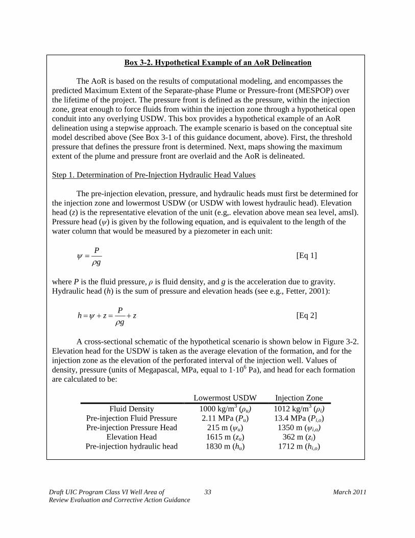
Draft UIC Program Class VI Well Area of 33 March 2011 Review Evaluation and Corrective Action Guidance
Box 3-2. Hypothetical Example of an AoR Delineation
The AoR is based on the results of computational modeling, and encompasses the predicted Maximum Extent of the Separate-phase Plume or Pressure-front (MESPOP) over the lifetime of the project. The pressure front is defined as the pressure, within the injection zone, great enough to force fluids from within the injection zone through a hypothetical open conduit into any overlying USDW. This box provides a hypothetical example of an AoR delineation using a stepwise approach. The example scenario is based on the conceptual site model described above (See Box 3-1 of this guidance document, above). First, the threshold pressure that defines the pressure front is determined. Next, maps showing the maximum extent of the plume and pressure front are overlaid and the AoR is delineated.
Step 1. Determination of Pre-Injection Hydraulic Head Values
The pre-injection elevation, pressure, and hydraulic heads must first be determined for
the injection zone and lowermost USDW (or USDW with lowest hydraulic head). Elevation head (z) is the representative elevation of the unit (e.g,. elevation above mean sea level, amsl). Pressure head (ψ) is given by the following equation, and is equivalent to the length of the water column that would be measured by a piezometer in each unit:
gρψ = P [Eq 1]
where P is the fluid pressure, ρ is fluid density, and g is the acceleration due to gravity. Hydraulic head (h) is the sum of pressure and elevation heads (see e.g., Fetter, 2001):
zg
Pzh +=+=ρ
ψ [Eq 2]
A cross-sectional schematic of the hypothetical scenario is shown below in Figure 3-2.
Elevation head for the USDW is taken as the average elevation of the formation, and for the injection zone as the elevation of the perforated interval of the injection well. Values of density, pressure (units of Megapascal, MPa, equal to 1·106 Pa), and head for each formation are calculated to be:
Lowermost USDW Injection Zone
Fluid Density 1000 kg/m3 (ρu) 1012 kg/m3 (ρi) Pre-injection Fluid Pressure 2.11 MPa (Pu) 13.4 MPa (Pi,o) Pre-injection Pressure Head 215 m (ψu) 1350 m (ψi,o)
Elevation Head 1615 m (zu) 362 m (zi) Pre-injection hydraulic head 1830 m (hu) 1712 m (hi,o)
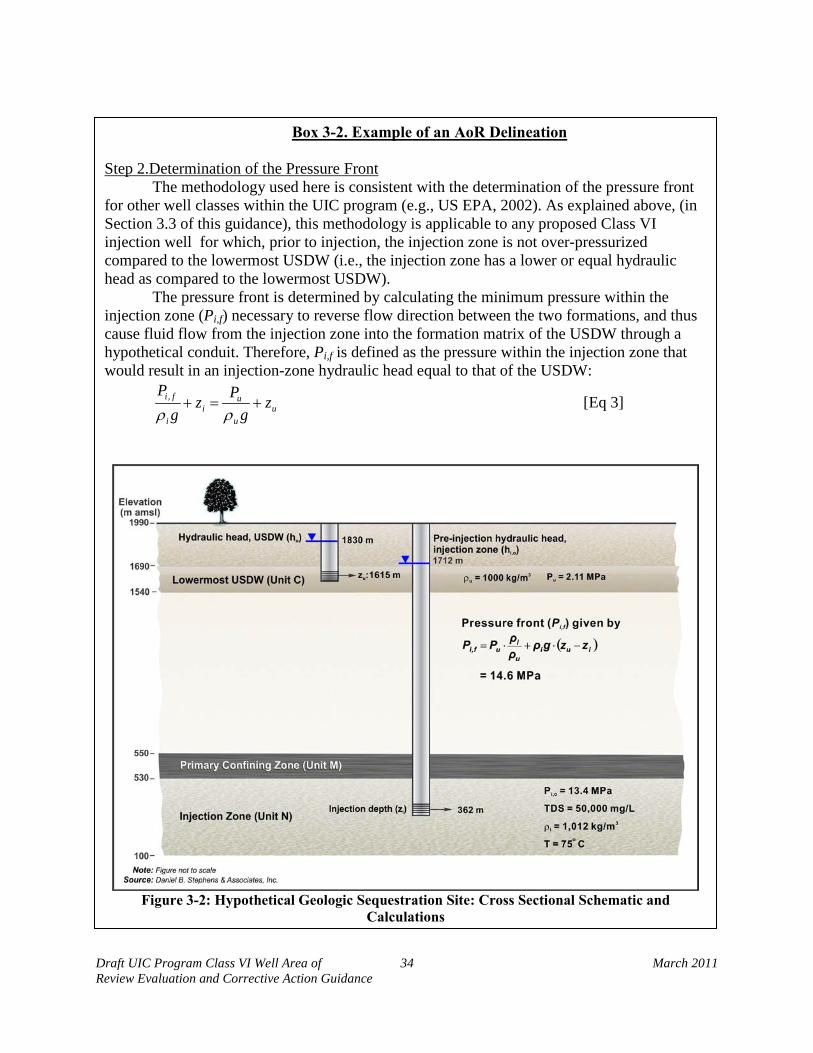
Draft UIC Program Class VI Well Area of 34 March 2011 Review Evaluation and Corrective Action Guidance
Box 3-2. Example of an AoR Delineation Step 2.Determination of the Pressure Front
The methodology used here is consistent with the determination of the pressure front for other well classes within the UIC program (e.g., US EPA, 2002). As explained above, (in Section 3.3 of this guidance), this methodology is applicable to any proposed Class VI injection well for which, prior to injection, the injection zone is not over-pressurized compared to the lowermost USDW (i.e., the injection zone has a lower or equal hydraulic head as compared to the lowermost USDW).
The pressure front is determined by calculating the minimum pressure within the injection zone (Pi,f) necessary to reverse flow direction between the two formations, and thus cause fluid flow from the injection zone into the formation matrix of the USDW through a hypothetical conduit. Therefore, Pi,f is defined as the pressure within the injection zone that would result in an injection-zone hydraulic head equal to that of the USDW:
uu
ui
i
fi zg
Pzg
P+=+
ρρ, [Eq 3]
Figure 3-2: Hypothetical Geologic Sequestration Site: Cross Sectional Schematic and
Calculations
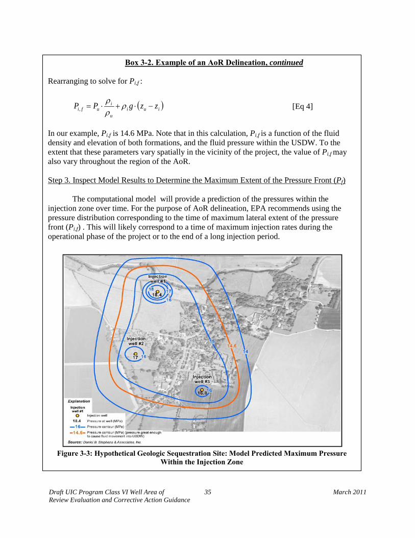
Draft UIC Program Class VI Well Area of 35 March 2011 Review Evaluation and Corrective Action Guidance
Box 3-2. Example of an AoR Delineation, continued
Rearranging to solve for Pi,f :
( )iuiu
iufi zzgPP −⋅+⋅= ρρρ
, [Eq 4]
In our example, Pi,f is 14.6 MPa. Note that in this calculation, Pi,f is a function of the fluid density and elevation of both formations, and the fluid pressure within the USDW. To the extent that these parameters vary spatially in the vicinity of the project, the value of Pi,f may also vary throughout the region of the AoR. Step 3. Inspect Model Results to Determine the Maximum Extent of the Pressure Front (Pf)
The computational model will provide a prediction of the pressures within the
injection zone over time. For the purpose of AoR delineation, EPA recommends using the pressure distribution corresponding to the time of maximum lateral extent of the pressure front (Pi,f) . This will likely correspond to a time of maximum injection rates during the operational phase of the project or to the end of a long injection period.
Figure 3-3: Hypothetical Geologic Sequestration Site: Model Predicted Maximum Pressure
Within the Injection Zone
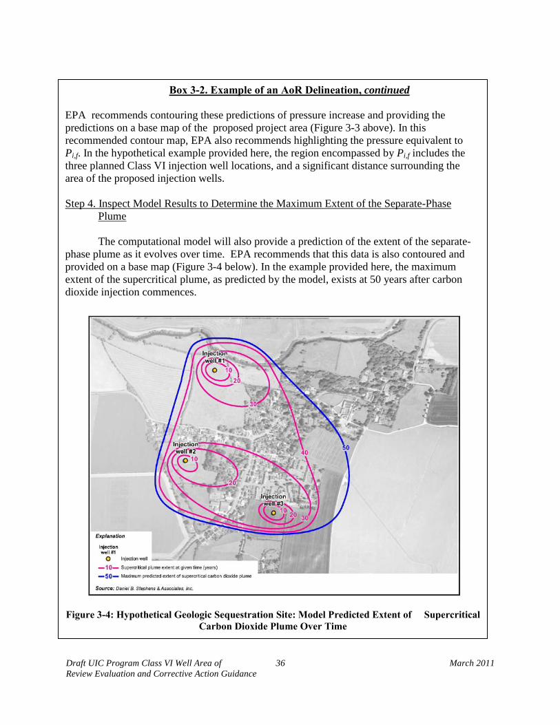
Draft UIC Program Class VI Well Area of 36 March 2011 Review Evaluation and Corrective Action Guidance
Box 3-2. Example of an AoR Delineation, continued
EPA recommends contouring these predictions of pressure increase and providing the predictions on a base map of the proposed project area (Figure 3-3 above). In this recommended contour map, EPA also recommends highlighting the pressure equivalent to Pi,f. In the hypothetical example provided here, the region encompassed by Pi,f includes the three planned Class VI injection well locations, and a significant distance surrounding the area of the proposed injection wells.
Step 4. Inspect Model Results to Determine the Maximum Extent of the Separate-Phase
Plume
The computational model will also provide a prediction of the extent of the separate-phase plume as it evolves over time. EPA recommends that this data is also contoured and provided on a base map (Figure 3-4 below). In the example provided here, the maximum extent of the supercritical plume, as predicted by the model, exists at 50 years after carbon dioxide injection commences.
Figure 3-4: Hypothetical Geologic Sequestration Site: Model Predicted Extent of Supercritical
Carbon Dioxide Plume Over Time
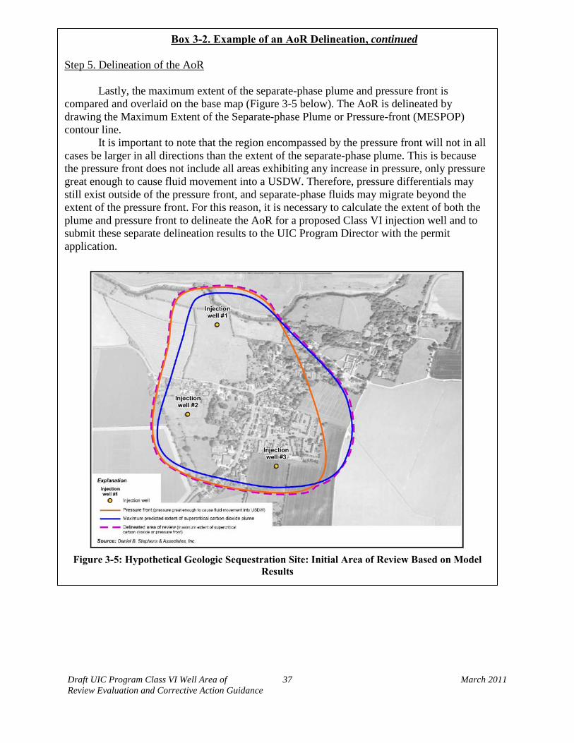
Draft UIC Program Class VI Well Area of 37 March 2011 Review Evaluation and Corrective Action Guidance
Box 3-2. Example of an AoR Delineation, continued
Step 5. Delineation of the AoR Lastly, the maximum extent of the separate-phase plume and pressure front is
compared and overlaid on the base map (Figure 3-5 below). The AoR is delineated by drawing the Maximum Extent of the Separate-phase Plume or Pressure-front (MESPOP) contour line.
It is important to note that the region encompassed by the pressure front will not in all cases be larger in all directions than the extent of the separate-phase plume. This is because the pressure front does not include all areas exhibiting any increase in pressure, only pressure great enough to cause fluid movement into a USDW. Therefore, pressure differentials may still exist outside of the pressure front, and separate-phase fluids may migrate beyond the extent of the pressure front. For this reason, it is necessary to calculate the extent of both the plume and pressure front to delineate the AoR for a proposed Class VI injection well and to submit these separate delineation results to the UIC Program Director with the permit application.
Figure 3-5: Hypothetical Geologic Sequestration Site: Initial Area of Review Based on Model
Results
Draft UIC Program Class VI Well Area of 38 March 2011 Review Evaluation and Corrective Action Guidance
However, as discussed previously, a single AoR modeling exercise may be conducted for all wells within a single project at the discretion of the UIC Program Director. In all cases, EPA recommends that the AoR delineation boundaries for the cumulative GS project be based on modeling that accounts for the anticipated injection rates from all planned Class VI injection wells.
3.4. Reporting AoR Delineation Results to the UIC Program Director
The owner or operator is required to submit the AoR and Corrective Action Plan with the initial stage of the permit application [§146.82 (a)]. Information pertaining to how this plan should be submitted is provided in the Draft UIC Program Class VI Well Project Plan Development Guidance. The final delineated AoR based on computational modeling is submitted to the UIC Program Director prior to authorization to inject [§146.82 (c)(1)]. EPA recommends that this permit application submittal include all necessary information for the UIC Program Director to evaluate the AoR delineation results and replicate the computational model exercise if he/she elects to do so, as well as all model input and output data and files. EPA recommends that the permit application submittal include the following in support of the AoR delineation:
The conceptual site model and all supporting data on which the model is based,
including the description of geologic stratigraphy and any relevant geologic features. See Box 3-1 of this guidance document for more information;
Attributes of the code used to create the computational model, including the code name, name of developing organization, a full accounting or reference to the model governing equations, scientific basis, and any simplifying assumptions;
A description of the model’s lateral and vertical extents, geologic layer thickness, and grid cell sizes, as presented on maps and cross-sections;
An accounting of all equations of state used for all fluids modeled (e.g. ground water, carbon dioxide);
Any constitutive relationships, such as relative-permeability saturation relationships, and how they were determined;
Values of all model parameters, as detailed in Table 2-1 of this guidance document, throughout the entire model domain, at all time steps during the model timeframe, including initial conditions and boundary conditions, and a description of how model parameters were determined based on site characterization data. This information may be submitted in tabular or graphical/map formats;
If required by the UIC Program Director, the owner or operator must also include raw model input and output files. These files may be useful in model verification, or if the UIC Program Director wishes to run alternative simulations/scenarios with the model;
Model results, including predictions of carbon dioxide and pressure-front migration over the lifetime of the project. EPA recommends that the model results be presented
Draft UIC Program Class VI Well Area of 39 March 2011 Review Evaluation and Corrective Action Guidance
in the form of maps, cross-sections, and/or graphs showing plume and pressure front migration as a function of time, and that the permit application submittal include maximum-risk scenario simulations and the outcome of parameter sensitivity analyses; and
If required by the UIC Program Director, the relevant qualifications and professional experience of any individuals and/or consulting firms responsible for model development, AoR delineation, and reevaluation, including examples of previous multiphase modeling studies conducted.
Draft UIC Program Class VI Well Area of 40 March 2011 Review Evaluation and Corrective Action Guidance
4. Identifying Artificial Penetrations and Performing Corrective Action
The purpose of AoR delineation for a proposed GS project is to determine the area where any geologic features or artificial penetrations (e.g., wells) may become conduits for fluid movement out of the injection zone, or additional zones, and potentially cause endangerment to a USDW. Within the delineated AoR for a Class VI injection well, any artificial penetrations that may penetrate the confining zone must be identified [§146.84(c)(2)]. Once identified, all wells must be evaluated for the quality of casing and cementing, and any of those identified wells that have been abandoned must be evaluated for the quality of plugging and abandonment in order to determine if they will remain properly sealed for the life of the sequestration project [§146.84(c)(3)]. Based on this evaluation, the owner or operator must perform corrective action on all artificial penetrations within the AoR that may cause a risk of endangerment to a USDW, including any abandoned wells that have been improperly plugged [§146.84(d)]. This section discusses the identification and evaluation of artificial penetrations, and performing the required corrective action if necessary. Monitoring activities necessary for detection of any fluid leakage into USDWs are discussed in the forthcoming Draft UIC Program Class VI Well Testing and Monitoring Guidance.
4.1. Identifying Artificial Penetrations within the AoR
The GS Rule requires potential Class VI injection well owners or operators to identify all artificial penetrations, including active and abandoned wells and underground mines, located within the delineated AoR that may penetrate the confining zone, and provide a description of each well’s type, construction, date drilled, location, depth, and if applicable, the record of plugging and/or completion, and any additional information the UIC Program Director may require [§146.84(c)(2)]. If the identified abandoned wells have been improperly plugged or not plugged at all, such penetrations can provide unimpeded flow conduits out of the injection zone. As such, they must be properly plugged in order to prevent endangerment of USDWs [§146.84(c)].
A variety of types of abandoned wells may exist within the delineated AoR of a proposed GS project, including wells constructed prior to Federal or state regulation (i.e., late 1800s or early 1900s), and any recently decommissioned wells. Wells constructed during early oil exploration, including cable-tool drilled wells, pose the largest risk because these wells may be relatively deep and often consist of an open (i.e., non-cased) wellbore over much of their length. These older wells may also not have been documented in state or local records.
Historically, wells no longer in use may not have been plugged and abandoned by today’s common standards. Prior to the early 1900s there were no regulations concerning well abandonment and it is unlikely that those wells were abandoned properly. Even in states regulating well abandonment, it is likely that any wells abandoned before 1952 may have inadequate plugs (Ide et al., 2006). In 1952, the American Petroleum Institute (API) published its standards for cements for oil and gas wells. Prior to that, cement often lacked sufficient additives to achieve the proper cement setting in the conditions experienced in oil and gas wells. As a
Draft UIC Program Class VI Well Area of 41 March 2011 Review Evaluation and Corrective Action Guidance
result, the plugs in many of these older wells failed to set properly and may have experienced channeling and/or cement failure because of fluid intrusion into the improperly set cement.
The potential also exists for more recently constructed wells to have been decommissioned improperly. For example, wells may have been plugged with debris and trash rather than with the proper cement. Depending on site conditions and corrosion, ‘properly’ plugged wells may also contain zones (i.e., annular spaces) that may serve as a conduit for fluid movement. In other cases, the well plugs may have degraded over time because of a poor cement job and/or corrosive conditions. Even properly plugged wells may have been plugged with types of cement that could degrade when in contact with a carbon dioxide plume. See the Draft UIC Program Class VI Well Construction Guidance for information on compatibility of different materials with a carbon dioxide stream.
Detecting abandoned wells can be very challenging in certain locations because of the variety of wells that may exist. In addition, steel casings, the primary detectable portion of the well, were often removed from abandoned wells for recycling and use during World War II (Gochioco and Ruev, 2006). These challenges are compounded by the potentially large AoR delineation determined for a proposed Class VI injection project, and therefore the greater surface area that will have to be evaluated for the presence of artificial penetrations. However, as discussed below, several methods and sources of information are available to identify those artificial penetrations in a relatively efficient manner. The primary stages of an abandoned well investigation within the AoR include historical research, site reconnaissance, review of aerial and satellite imagery, and one or more geophysical surveys. The reader is referred to additional standard references regarding identification of artificial penetrations for further information (Jordan and Hare, 2002; Frischknecht et al., 1985, ASTM, 2005).
4.1.1. Historical Research
Most deep wells that may penetrate the primary confining zone of a proposed GS project site are related to oil and gas exploration and production. Deep well drilling for oil and gas exploration dates back to the 1870s. State and local databases of well exploration may include locations of abandoned wells, and EPA recommends conducting a records review as the first step in abandoned well identification within the delineated AoR for a proposed Class VI injection well. In addition, state and local records will provide information on the time period and types of oil exploration that have been conducted in an area, and may also provide information on typical completion and abandonment methods in a given field. This records search will provide a list of known abandoned wells, and may also inform additional stages of abandoned well identification.
State well databases will, in most cases, provide valuable information for assistance with the identification of abandoned wells. Prior to well construction, a government permitting authority requires owners or operators to seek a permit to drill, either with a Natural Resources Agency, Environmental Quality Agency, or Geological Survey. Most states maintain records of drilled wells, including location, construction, operating, and plugging information. Although these records can take many forms, many states now have comprehensive databases of these well records that have been digitized and made available online. However, when conducting this historical records search, owners and operators of proposed Class VI injection wells should be
Draft UIC Program Class VI Well Area of 42 March 2011 Review Evaluation and Corrective Action Guidance
aware that older well records may not have been entered into these databases. In some cases, the records from different time periods may be filed in separate locations or on separate types of media.
For example, the Wyoming Oil and Gas Conservation Commission maintains a digital database accessible online, of wells within the state. See http://wogcc.state.wy.us for more information on this database. Basic information is available to the public regarding each well, as well as the geophysical survey results where available. This database can be searched by location, name, and well number, among other fields. The state also has a “well book” available on line, which contains records of older wells not entered in the database.
In addition, county records, including survey maps, ownership records, chain-of-title and property lease history, maintained by local tax assessors and country clerks, in many cases list abandoned wells. Such records may also indicate land use and indicate areas and time frames where drilling activities likely occurred. Private data compilation services often maintain detailed databases for the purpose of oil and gas exploration, including information regarding well locations, plugging, and abandonment. Often these services will maintain maps of known well locations. While these maps can be out of date, most private services have been known to update their database for a fee.
4.1.2. Site Reconnaissance
Site reconnaissance includes interviewing local residents and property owners, as well as conducting a physical search for features indicative of abandoned wells. Initial site reconnaissance may be informed by the historical database research. For example, the records search may indicate that, with a great deal of confidence, certain regions of the AoR have never been subject to oil and gas exploration, deep well injection, or any other activity that may result in deep well penetration. In this case, the owner(s) or operators(s) may choose to exclude those areas from any additional well identification efforts.
Local residents that may be well-informed regarding abandoned wells include oilfield workers and service company employees, including consultants, and property and drilling-rights ownership brokers. Such informed residents may be able to give information on the areas and time frames where past drilling occurred. They may also be able to give more specific details in response to specific questions and provide information on locations, completion methods, and plugging of wells.
Surface features that may be indicative of abandoned wells include abandoned well derricks, access roads, brine pits, or vegetation stress associated with brine leakage. Detection of these features at a site indicates the possible likelihood of one or more wells in the area. EPA recommends that, because the AoR is likely to cover a large area, a surface review for such features is most effectively supplemented by use of aerial surveys or photos, as discussed below.
Draft UIC Program Class VI Well Area of 43 March 2011 Review Evaluation and Corrective Action Guidance
4.1.3. Aerial and Satellite Imagery Review
EPA recommends that historical aerial photographs and satellite imagery be used in the identification of abandoned wells. Aerial photographic surveys, taken from airplanes, were conducted beginning in the 1930s, and are available from a variety of governmental and private information services. All historical aerial photos within the AoR are recommended to be reviewed for evidence of past drilling activity. Surface features that provide a ‘signature’ of drilling activity include drill derricks, rig platforms, brine pits, power sources, and access roads.
Satellite (i.e., remote sensing) images do not have the resolution to detect individual objects, such as wellheads or derricks, but can be used to detect surface features indicative of abandoned wells. These include spatial patterns indicative of a well site, brine pits, modified topography, and vegetation stress associated with brine leakage. See Jordan and Hare (2002) for more information regarding accessing and interpretation of satellite imagery.
4.1.4. Geophysical Surveys
Geophysical surveys, including magnetic, ground penetrating radar (GPR), and electromagnetic methods, can be used in the detection of abandoned wells. Geophysical surveys are recommended to be conducted throughout regions of the AoR that may have been subject to oil and gas exploration, deep well injection, or any other activity that may result in deep well penetration. Geophysical methods will supplement other identification methods, discussed above. Geophysical methods can help to pinpoint locations of known wells where surface evidence of the well has been removed or can help to identify abandoned wells that are undocumented. The type(s) of geophysical surveys conducted at a proposed Class VI injection well site are based on known site subsurface and surface conditions. In general, at least two different types of geophysical surveys are recommended in order to parse data background noise and to inform the interpretation of survey results. As discussed below, ground or aerial (e.g., aeromagnetic) surveys may be conducted, depending on the size of the area of interest.
4.1.4.1. Magnetic Methods
The magnetic method is one of the oldest and most well developed geophysical techniques, and is the standard method used for abandoned well detection. Magnetic surveys measure a component of the magnetic field near the land surface. Any anomalies in the magnetic field are caused by subsurface features, which could include any abandoned wellbores with iron or steel casings. Anomalies associated with well casings are typically distinguishable from the background magnetic field.
Magnetic surveys are applicable to abandoned wells with iron or steel casings or to wellheads in areas with relatively low background magnetic signatures. Areas with significant cultural development on the surface or in the shallow subsurface may have high interferences. Airborne magnetic surveys can detect most wells constructed with approximately 200 feet or more of at least 8-inch casing, and in some cases, very large cavities (Frischknecht et al., 1985). However, open wellbores, non-steel casings, or severely corroded casings cannot typically be detected with a magnetic survey.
Draft UIC Program Class VI Well Area of 44 March 2011 Review Evaluation and Corrective Action Guidance
Ground or aerial (i.e., aeromagnetic) surveys may be conducted, depending on the size of the area of interest. Aeromagnetic surveys will likely be more practical for most GS projects due to the anticipated size of the delineated AoR, as they can collect large amounts of data in a relatively short amount of time. Both ground and aerial surveys are conducted along straight-line transects. EPA recommends that that ground survey transect spacing be no larger than 20-30 feet, and aerial survey transect spacing be no larger than 50-100 feet (Jordan and Hare, 2002).
Magnetic surveys may be conducted to measure the total magnetic field, or the vertical or horizontal field gradients. For the purpose of locating abandoned wellbores, the total magnetic field measurement type is recommended. During these surveys, EPA recommends that the operator avoid placing magnetic materials or interfering materials near the magnetometer, periodically return to a common point to ensure instrument repeatability, continuously measure diurnal variation in the magnetic field, and avoid high-magnetic gradients. Data processing of magnetic surveys includes incorporation of spatial positioning data, correction for diurnal variation, and data filtering.
Figure 4-1 of this guidance, below, compares aeromagnetic survey results for the Coon Creek oil field in Oklahoma to identified abandoned wells from aerial imagery (USGS, 1995). As shown in the figure, magnetic anomalies associated with well casings are typically apparent. However, this figure also reveals some of the typical challenges that may be faced by owner(s) or operator(s) in abandoned wellbore identification. One challenge is that due to the presence of other buried infrastructure (e.g., pipes) certain regions exhibit larger magnetic field values even if wells are not present. Additionally, some wells may not be identified in the aeromagnetic survey, most likely because of well casing removals. These challenges demonstrate the benefits of using multiple survey techniques in order to properly identify abandoned wells.
4.1.4.2. Electromagnetic Methods
Electromagnetic methods used for abandoned wellbore detection include frequency domain and time domain electromagnetic surveys. These surveys consist of an electromagnetic transmitter that establishes an electromagnetic field measured by a receiver. Similar to magnetic surveys, electromagnetic surveys are non-invasive, as both the transmitter and receiver are positioned above the ground surface. Both surface and aerial electromagnetic surveys are possible. The depth at which these instruments are able to detect objects depends on the size and geometry of the sensor, the size and conductivity of the target, and the potential interference from other sources, such as fences and pipelines. Generally, object detection at depths ranging from a few meters to several hundred meters is possible. Larger and more complex arrays are required at greater depths. Aerial surveys are not likely able to detect small objects, such as well casings, but may detect brine plumes, which may indicate the presence of abandoned wells (Jordan and Hare, 2002).
Abandoned wellbore detection using electromagnetic methods is based on the larger conductivity of steel casings and other well materials compared to surrounding soils and geologic formations. These methods may detect anomalous fluids associated with leakage from an abandoned well. Frequency domain electromagnetic methods can measure current induced in the subsurface by

Draft UIC Program Class VI Well Area of 45 March 2011 Review Evaluation and Corrective Action Guidance
the electromagnetic field established by the transmitter. Induced current establishes a secondary electromagnetic field detected by the receiver. The magnitude of the induced current is a function of subsurface conditions, including conductivity. Time-domain electromagnetic methods measure the decay of the secondary magnetic field created by the induced current, and can be especially useful for detection of brine leakage.
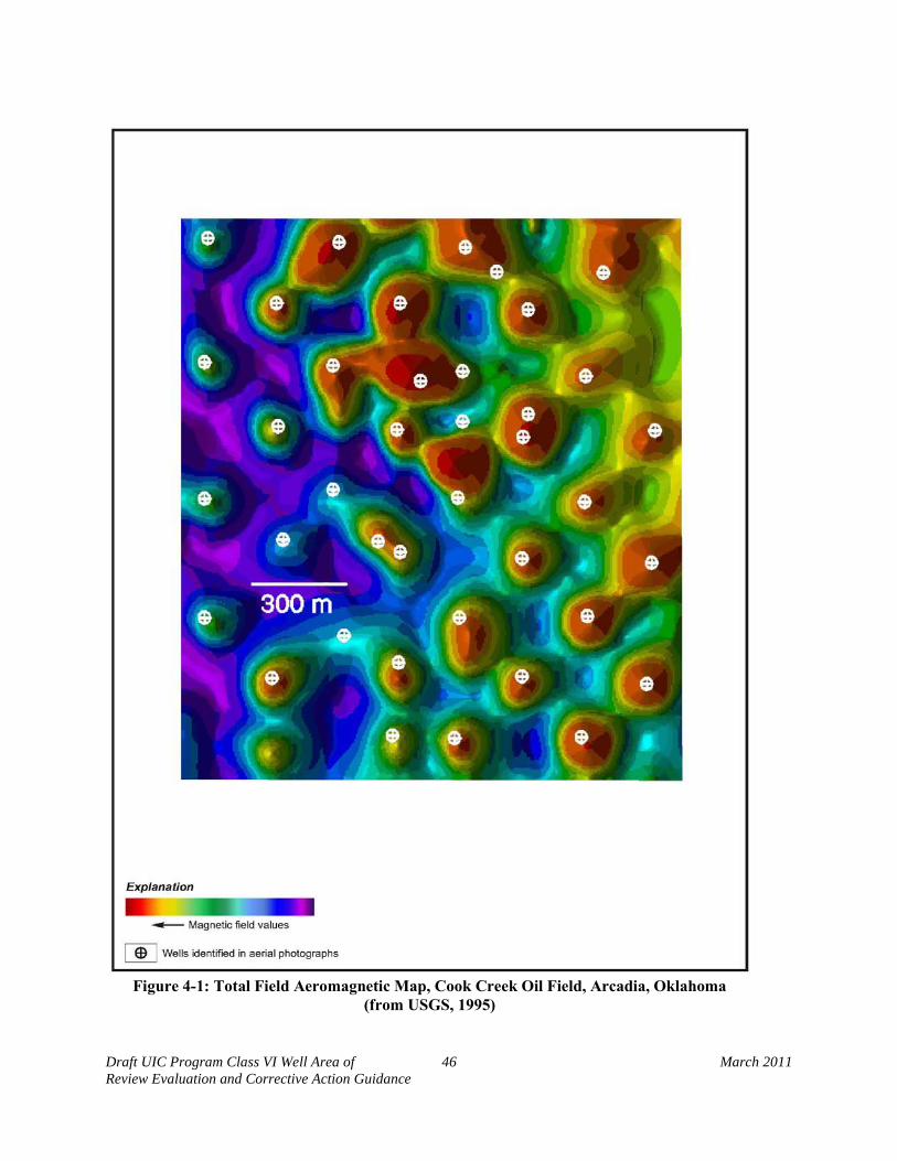
Draft UIC Program Class VI Well Area of 46 March 2011 Review Evaluation and Corrective Action Guidance
Figure 4-1: Total Field Aeromagnetic Map, Cook Creek Oil Field, Arcadia, Oklahoma
(from USGS, 1995)
Draft UIC Program Class VI Well Area of 47 March 2011 Review Evaluation and Corrective Action Guidance
4.1.4.3. Ground Penetrating Radar
Ground penetrating radar (GPR) may be used in abandoned wellbore detection and in finding other artificial penetrations. Unlike other geophysical methods, GPR does not rely on the presence of a steel or iron wellbore, so it may be able to detect open boreholes and non-metallic materials. GPR uses high frequency radio waves to measure the transmission of electromagnetic energy. The investigation depth possible depends on the frequency of the radio waves and the conductivity of the ground. The greater the depth the less resolution the instrument will have. For small objects, such as well casings, depths are limited to a few meters (Jordan and Hare, 2002). GPR is also slower than magnetic or electromagnetic methods.
GPR is likely not as practical to use throughout the delineated AoR as an initial larger scale survey method because the distance between transect lines for sufficient resolution is too small. Instead, EPA recommends using GPR to determine the exact location of abandoned wellbores within a given area that have already been identified by earlier larger scale surveys.
4.2. Assessing Identified Abandoned Wells
After all artificial penetrations within the AoR that may penetrate the confining zone have been identified, the owner(s) or operator(s) of a proposed Class VI injection well must evaluate the potential for each artificial penetration to serve as a conduit for fluid movement [§146.84(c)(2)]. In particular, owners or operators must establish which abandoned wells in the AoR, if any, have not been plugged in a manner that would prevent the movement of carbon dioxide or other fluids that may endanger USDWs [146.84(c)(3)]. To prevent fluid movement, abandoned wells should include a cement plug through the primary confining zone, and/or across the injection zone/confining zone contact, with sufficient integrity to contain separate-phase carbon dioxide and elevated pressures. In the absence of an adequate plug across the confining zone, cross-migration may occur where fluids enter a permeable zone below the lowermost USDW and then migrate upward from that zone. See Figure 4-2 of this guidance document, below, for more information. EPA recommends cement surface plugs (typically required by well abandonment regulations), and the UIC Program Director may require additional plugs based on site-specific circumstances.
Evaluation of the wells in the AoR requires a two step approach. The first step is to review whatever records are available, as outlined in Section 4.2.1, below, for information relevant to proper plugging. The second step is to perform physical tests on wells that are suspect or for which no records are available.
4.2.1. Abandoned Well Plugging Records Review
A records review can aid in reducing the number of identified wells that may need to be evaluated by future field testing. Records of wells that have been recently abandoned, have no mentions of any difficulties experienced during the abandonment procedure, are cased holes, and have plugs and cement situated to isolate the injection zone from other fluid containing zones may be used to justify reduction in the number of follow up field investigations. On the other hand, the records may be incomplete or may indicate that the well has not been plugged or was
Draft UIC Program Class VI Well Area of 48 March 2011 Review Evaluation and Corrective Action Guidance
inadequately plugged, and follow up field investigations may therefore be necessary. Identified undocumented wells will have no records and will require field investigation in order to determine the quality of plugging, as required in the GS Rule [§146.84(c)(3)].
There are many elements in existing reports that can help in determining the adequacy of abandonment procedures for identified wells located within the AoR. Some key elements to review include, but are not limited to:
Well depth and completion, Well abandonment date, Open hole or cased hole, Location of plugs, Casing and cementing records, Records of MITs, or logs performed, and Well deviation.
The well completion depth is important in determining if the identified abandoned well may penetrate the proposed confining zone(s). If the well completion depth is above the confining zone(s), no further action would likely need to be taken. The date of abandonment may also provide information as to the adequacy of the abandonment procedure. Whether the well was abandoned with casing or as an open hole is an important consideration in determining the likelihood that the well might act as a conduit for fluid movement. Open holes are susceptible to cross migration between aquifers. If the hole is open and there is not a proper plug located at a depth corresponding to the primary confining zone, fluids may migrate out of the injection zone and into a USDW. For cased holes, EPA recommends that integrity of the casing be evaluated.
The location and type of plugs are also important factors, especially in open-hole wells. The plug locations must be reviewed in order to determine the quality of plugging, as required in the GS Rule [§146.84(c)(3)]. For example, EPA recommends that the injection zone be isolated from all other formations with plugs. This may be especially important if a well was completed in a formation deeper than the proposed injection zone. EPA recommends that any length of the well in the proposed injection zone be properly isolated by means of plugs and casing. Mechanical plugs and cemented casing are not sufficient for the long term isolation of carbon dioxide, as eventually the metal is likely to corrode and the plug will fail (Randhol et al., 2007). Therefore, cement plugs are considered superior to mechanical plugs for preventing the movement of fluids into or between USDWs. EPA recommends that cement plugs be located across the bottom of any casings, at the base of the lowermost USDW, and that plugging fluid (i.e., composition, specific gravity) characteristics be considered, as drilling fluid of sufficient weight may resist displacement by the injectate or mobilized fluids.
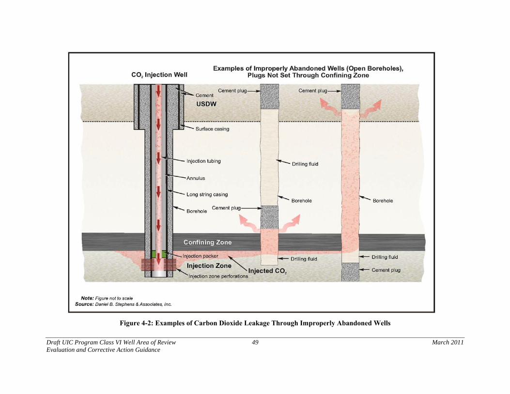
Draft UIC Program Class VI Well Area of Review 49 March 2011 Evaluation and Corrective Action Guidance
Figure 4-2: Examples of Carbon Dioxide Leakage Through Improperly Abandoned Wells
Draft UIC Program Class VI Well Area of 50 March 2011 Review Evaluation and Corrective Action Guidance
The integrity of any existing casing and cement must be determined in order to assess the quality of well construction and plugging, as required in the GS Rule [§§146.84(c)(2) and 146.84(c)(3)]. EPA recommends reviewing the casing and cement quality through the proposed injection zone in order to ensure that they are appropriate for contact with carbon dioxide, and any additional well records that indicate any unusual conditions experienced during casing and cementing. Any recorded events such as a loss of circulation, wellbore stability problems, lack of the use of centralizers, and/or improper removal of drilling mud before cementing can all lead to premature cement or casing failure. If available, reviewing load calculations and comparing them to actual events recorded in the drilling log may give the owner(s) or operator(s) an indication of an under designed casing that may be susceptible to failure. For example, if the casing had a low axial loading stress and stuck pipe was experienced during casing placement, it is possible that the casing may have experienced damage. The materials used for the well casing and cement must also be assessed to see if they are compatible with carbon dioxide, in order to comply with GS Rule requirements [§146.84(c)(3)]. See the Draft UIC Program Class VI Well Construction Guidance for more information on compatibility of different materials with a carbon dioxide stream.
Any tests performed on the well prior to its abandonment can also be useful information. A mechanical integrity test (MIT) such as a pressure test, noise log, temperature log, or cement bond log can provide information on any known or suspected leaks. If leaks were encountered, EPA recommends determining if the source of the leak was found and repaired. If the leaks were not sealed, corrective action would be required to be taken to plug the leaks as discussed below [§146.84 (d)]. Drilling records can yield clues as to areas that might be susceptible to failure. Mud logs and open-hole caliper logs can show areas of weak formations. Weak formations are susceptible to wellbore instability and subsequent cement failure. Cement bond logs and temperature logs taken at the time of completion can also give an idea of the condition of the cement, although degradation is always possible after well completion. Any corrosion logs will help provide information on the condition of the casing. Results from mechanical caliper logs, electromagnetic thickness logs, or down-hole video can show the casing condition when the well was abandoned. For more information regarding these logs and tests, see the forthcoming Draft UIC Program Class VI Well Testing and Monitoring Guidance.
Evaluation of well records for deviation during drilling may also identify wells more likely to be in need of corrective action, as deviated wells are far more likely to fail than wells with no deviation (Watson, 2009). Events, such as wellbore collapse during drilling or conditions that placed unusual loads on the casing, may also indicate a higher chance of failed wellbore integrity. EPA recommends that the design casing load also be checked to ensure adequacy for the actual loads faced by the well.
4.2.2. Abandoned Well Field Testing
After all the available records have been reviewed, any wells located within the AoR that cannot be proven to have adequate plugs must be evaluated by field tests in order to determine the quality of plugging, as required in the GS Rule [§146.84(c)(3)]. If the integrity of the bottom plug or cement is in question, and records cannot prove that the plugging is adequate, EPA recommends that the surface plug and possibly additional plugs down-hole be drilled out and
Draft UIC Program Class VI Well Area of 51 March 2011 Review Evaluation and Corrective Action Guidance
tests conducted to determine the adequacy of abandonment. There are numerous field tests available to evaluate the integrity of abandoned wells. Several of these tests are discussed in detail in the forthcoming Draft UIC Program Class VI Well Testing and Monitoring Guidance. Additionally, the owner or operator must demonstrate guaranteed site access to wells potentially needing corrective action in the future [§146.84(b)(iv)]. The owner or operator is encouraged to consult the UIC Program Director regarding any difficulties in gaining site access in order to evaluate and perform corrective action on any identified improperly plugged abandoned wells.
EPA recommends that both the casing and the cement plugs be evaluated. Casing failure is most common at joints and in weak formations where instability around the wellbore can lead to failed cement and to casing buckling. Weak formations are also common areas for cement failure, as are high pressure formations, due to fluid intrusion. Tools used to evaluate the cement and casing include, but are not limited to:
Multi-finger caliper log, Sonic scanner, Ultrasonic imaging tool, Cement bond log, Radioactive tracer, Cased hole dynamic tester, Modular sidewall coring tool, and a Cased hole fluid test.
Multi-finger caliper logs measure the radius of the borehole in a non-destructive way. They can give a 360-degree picture of the inside of the casing and identify any defects caused by corrosion, erosion, or other events (e.g. dropped tools).
A sonic scanner sends out sound waves and measures the returned waves in receivers. The log provides information on the quality of the casing-cement bond and the cement-formation bond. The sonic scanner averages the results for the entire radius and therefore cannot provide three-dimensional pictures of the cement bond, or determine the reasons for a poor quality cement bond. An ultrasonic imaging tool is another non-destructive tool that uses ultrasonic transmitters and receivers to determine information about the casing and cement. The ultrasonic imaging tool can return 360-degree information on casing thickness, cement thickness, and cement bond. More information on these tools can be found in Duguid and Crow (2007) and Close et al. (2009).
A cement bond log is another tool used and log results include information on both the cement and the bond quality. This log provides results that are averaged over the circumference of the well, and testing is typically conducted in combination with an ultrasonic imaging tool to provide more complete information on the three-dimensional picture of the well. In some cases, the cement hardens while the well casing is under pressure, and when pressure is released, microannuli can form between the casing and cement. If unconnected to other cracks, these microannuli cannot transmit fluid, but will show up in logging results as a potential poor bond. This artifact can be evaluated by performing the cement bond log under pressure (Randhol et al., 2007). Radioactive tracers also can be used to detect leaks in casing and cement and fluid leaking
Draft UIC Program Class VI Well Area of 52 March 2011 Review Evaluation and Corrective Action Guidance
along channels in the wellbore. Radioactive tracers are injected down the well, and gamma detectors are used to detect any fluid flow.
Cased-hole dynamic testers measure mobility or porosity. They can be used to determine the porosity of the cement. They are semi-destructive tests as they do create a small hole in the casing and cement; however, the hole is patched after the test is run. The instrument works well in highly permeable formations or in cement, while performance in lower porosity formations is still under investigation.
Modular sidewall coring tools take small cores of the casing and cement for analysis in the laboratory. Laboratory analyses can include scanning electron microscopy, X-ray diffraction, and measurements of permeability and density. This is a more destructive test that leaves approximately 1-inch diameter holes in the side of the well, which is then patched with a remedial cement squeeze after testing is completed. Cased-hole fluid testers can be run with the cased-hole mobility tool, using optical instruments to determine what fluids are present in the formation outside the wellbore. In general, EPA recommends that these tests be run sequentially from the simplest and least destructive to the more complicated and destructive tests. This way, if a flaw is found with a simpler test that determines that the well should be plugged or otherwise remediated, the more expensive and destructive tests may be avoided. The typical order of running the tests is caliper log, sonic and ultrasonic tools, cased-hole mobility and fluid tests, and then sidewall cores (Duguid and Crow, 2007). This set of tools can be used to determine the quality of the casing and cement, and if flaws such as degraded cement porosity, casing corrosion, microannuli in the cement, channels between the cement and casing or cement and formation, or missing cement are found, the GS Rule requires that corrective action be performed on the well by plugging and/or remedial cementing [§146.84(d)]. A brief summary of the main methods for evaluating cement and casing condition along with major benefits and disadvantages are included in Table 4-1 of this guidance document below.
4.3. Performing Corrective Action on Wells Within the AoR
The GS Rule requires that owners or operators of Class VI injection wells perform corrective action on all artificial penetrations in the AoR that may penetrate the confining zone, and are determined to have been plugged and abandoned in a manner such that they could serve as a conduit for fluid movement and endanger USDWs [§146.84(d)]. In performing corrective action, owners or operators must use methods designed to prevent the movement of fluid into or between USDWs, including use of materials compatible with the carbon dioxide stream, where appropriate [§146.84(d)].
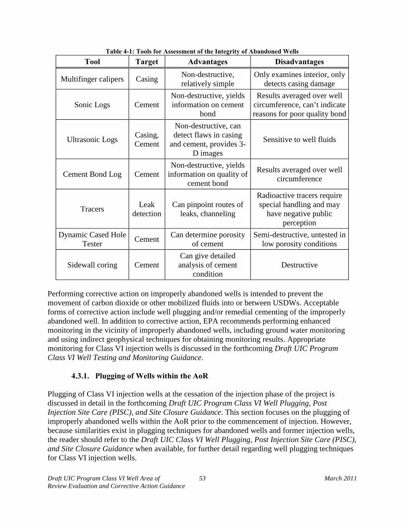
Draft UIC Program Class VI Well Area of 53 March 2011 Review Evaluation and Corrective Action Guidance
Table 4-1: Tools for Assessment of the Integrity of Abandoned Wells Tool Target Advantages Disadvantages
Multifinger calipers Casing Non-destructive, relatively simple
Only examines interior, only detects casing damage
Sonic Logs Cement Non-destructive, yields information on cement
bond
Results averaged over well circumference, can’t indicate reasons for poor quality bond
Ultrasonic Logs Casing, Cement
Non-destructive, can detect flaws in casing
and cement, provides 3-D images
Sensitive to well fluids
Cement Bond Log Cement Non-destructive, yields
information on quality of cement bond
Results averaged over well circumference
Tracers Leak detection
Can pinpoint routes of leaks, channeling
Radioactive tracers require special handling and may
have negative public perception
Dynamic Cased Hole Tester Cement Can determine porosity
of cement Semi-destructive, untested in
low porosity conditions
Sidewall coring Cement Can give detailed analysis of cement
condition Destructive
Performing corrective action on improperly abandoned wells is intended to prevent the movement of carbon dioxide or other mobilized fluids into or between USDWs. Acceptable forms of corrective action include well plugging and/or remedial cementing of the improperly abandoned well. In addition to corrective action, EPA recommends performing enhanced monitoring in the vicinity of improperly abandoned wells, including ground water monitoring and using indirect geophysical techniques for obtaining monitoring results. Appropriate monitoring for Class VI injection wells is discussed in the forthcoming Draft UIC Program Class VI Well Testing and Monitoring Guidance.
4.3.1. Plugging of Wells within the AoR
Plugging of Class VI injection wells at the cessation of the injection phase of the project is discussed in detail in the forthcoming Draft UIC Program Class VI Well Plugging, Post Injection Site Care (PISC), and Site Closure Guidance. This section focuses on the plugging of improperly abandoned wells within the AoR prior to the commencement of injection. However, because similarities exist in plugging techniques for abandoned wells and former injection wells, the reader should refer to the Draft UIC Class VI Well Plugging, Post Injection Site Care (PISC), and Site Closure Guidance when available, for further detail regarding well plugging techniques for Class VI injection wells.
Draft UIC Program Class VI Well Area of 54 March 2011 Review Evaluation and Corrective Action Guidance
Where records indicate that an abandoned well was not plugged, or was plugged and abandoned improperly, the well requires plugging in order to prevent fluid movement [§146.84(d)]. In addition, where records indicate that a well plug does not exist at a depth corresponding to the primary confining layer of the GS project, EPA recommends that the well have an additional plug set at this depth to meet the requirements of the GS Rule. Where records indicate that there are no well plugs below USDWs or other permeable formations that may exhibit cross flow of mobilized fluids, additional plugs may be required by the UIC Program Director for proper corrective action in these zones. Also, in wells that were plugged but the evaluation techniques discussed in Section 4.2 of this guidance document reveal cracks, channels, or annuli in the plug that would allow fluid migration, EPA recommends drilling out and replacing the plug. In addition, if the plug material may corrode in a carbon-dioxide rich environment, EPA recommends replacing it. For wells where casing exists at depths corresponding to the injection and/or confining zone and the annular space may serve as a conduit for fluid movement if not properly cemented, remedial cementing may be necessary or the casing may need to be removed and replaced with a cement plug. See Section 4.3.2 of this guidance document for more information on remedial cementing.
For the plugging of improperly abandoned wells within the AoR, EPA recommends that a plug be set at a depth interval corresponding to the primary confining zone overlying the injection zone of the Class VI injection well. In the absence of an adequate plug across the confining zone, cross-migration may occur wherein fluids enter a permeable zone below the lowermost USDW and then migrate upward from that zone. See Figure 4-2 of this guidance document for more information. However, in order to supplement the confining-zone plug, ideal additional plugging zones include the bottom of any casings, and across any USDWs. A surface plug would also typically be required by local well abandonment regulations to ensure that there is no risk of anyone physically falling into the wellbore.
To provide the best possible barrier to carbon dioxide migration out of the injection zone, EPA recommends that corrective action be conducted in a manner to provide multiple barriers to carbon dioxide migration, and avoid underground cross-flow. Materials that are compatible with the carbon dioxide are required to be used where appropriate [§146.84(d)]. Material compatibility with carbon dioxide is discussed further in the Draft UIC Program Class VI Well Construction Guidance.
4.3.2. Remedial Cementing
Properly cementing improperly abandoned wells located within the delineated AoR between any existing well casing and the geologic formation, especially through the injection zone, provides an important fluid migration barrier. EPA recommends performing remedial cementing in order to meet the corrective action requirements of the GS Rule if a well has been properly plugged but the records, or any testing such as that described in Section 4.2 of this guidance, indicate that the cement surrounding the wellbore has failed or has cracks, channels, or annuli that could allow migration of carbon dioxide [§146.84(2)(d)]. Key areas on which to focus remedial cementing include depths corresponding to the injection zone and through any other permeable zones.
Draft UIC Program Class VI Well Area of 55 March 2011 Review Evaluation and Corrective Action Guidance
Remedial cementing is performed through squeeze cementing, where the cement is emplaced into the affected area. For more information on cement squeezes, refer to Reynolds and Kiker (2003). Increased pressure on the cement forces water out of the cement slurry leaving behind the partially dehydrated cement. Cement squeezes can either be low pressure or high pressure. Low pressure squeezes are used to set a small amount of cement in a given area and operate at a pressure lower than the fracture pressure of the formation. Higher pressure squeezes are used when channels or disconnected microannuli are to be cemented. The higher pressure squeezes may fracture the formation and then allow the cement to flow into disconnected channels.
Cement squeezes can be performed using either a packer or a bradenhead squeeze. The methods differ in how the treated section is isolated from the rest of the well. In the packer squeeze, packers isolate the area to be treated, and a bridge plug isolates the area below the area to be cemented, while a modified packer with a bypass valve isolates the area above the treated area. Cement retainers are used if significant back pressure is expected. A bradenhead squeeze only isolates the area below the area to be cemented. It is typically used only if the casing above the treated area is strong enough to withstand the squeeze pressure. In cement squeezes, either drillable packers or retrievable packers can be used. Drillable packers allow less freedom in placement but better control of the cement. They are preferred if high pressures are maintained on the cement after the squeeze.
Cements used in squeeze cementing can vary depending on the nature of the defect. The GS Rule requires that all materials used for cementing of abandoned wells be compatible with the carbon dioxide stream, where appropriate [§146.84(d)]. Traditional cements may be supplemented with or replaced by materials such as polymer gels and acrylic grouts. Acrylic grouts can be used for small casing leaks or cases where pressure leak off is detected. High concentration low molecular weight polymers can be used for small to moderate leaks. High molecular weight polymers are typically used for channeling and lost circulation applications. Cement or cement/polymer blends are typically used for severe leaks (Randhol et al., 2007).
4.4. Reporting Well Identification, Assessment, and Corrective Action to the UIC
Program Director
As discussed in the Draft UIC Program Class VI Well Project Plan Development Guidance , the AoR and Corrective Action Plan, submitted with the initial stage of the permit application, must indicate what well identification and assessments will be used, and how corrective action will be conducted [§146.84(b)(2)(iv)]. The plan is a condition of the permit, and is subject to UIC Program Director approval [§146.84(b)].
Owners or operators seeking a Class VI injection well permit are required to report, with the full permit application, the following information regarding abandoned wells within the AoR that may penetrate the primary confining zone: the well’s type, construction, date drilled, location, depth, record of plugging and/or completion, and any additional information required by the UIC Program Director [§146.82(a)(4)]. This information can be found in acceptable public and private databases, where available. See Section 4.1.1. of this guidance, above, for more information. In cases where available records do not provide the necessary information, or indicate that the well was plugged improperly, in a questionable manner, or with materials
Draft UIC Program Class VI Well Area of 56 March 2011 Review Evaluation and Corrective Action Guidance
inappropriate for contact with carbon dioxide, then site investigations must be performed to establish the condition of the well, as discussed previously[§146.84(c)(3)].
The UIC Program Director will review the submitted well information to ensure completeness, and may consult with officials at oil and gas or water agencies to ensure that the well search was thorough. The UIC Program Director will also review well completion records to determine those wells that may penetrate the primary confining zone, and will likely compare this list to wells scheduled for corrective action and submitted with the Class VI injection well permit application. For those identified abandoned wells that have been determined by the owner(s) or operator(s) to not require corrective action, the UIC Program Director will likely review the records of plugging and any field testing conducted, to verify that the well does not require corrective action. If information on the depth or condition of the plug(s) is missing, the UIC Program Director may request additional tests or require the well to be re-plugged.
Reports of any tests done on abandoned wells must be submitted to the UIC Program Director with the permit application along with a list of wells for which corrective action will be conducted [§146.84(c)(2)]. On completion of corrective action activities, the reports indicating the number, type, and location of the plugs must be submitted to the UIC Program Director [§146.84(c)(2)]. Records of any remedial cementing are also recommended to be submitted with the Class VI injection well permit application along with cement logs showing the methods used and the results of the remedial cementing.
4.5. Use of Phased Corrective Action
At the Discretion of the UIC Program Director, the owner or operator may perform corrective action for Class VI injection wells in a phased manner [§146.84(b)(2)(iv)]. This means that prior to injection, artificial penetrations are identified throughout the delineated AoR, and submitted with the Class VI injection well permit application information, but the appropriate corrective action is first conducted only in the portions of the delineated AoR closer to the injection well(s). Corrective action activities in more distant portions of the AoR can be conducted in later phases of the GS project. Phased corrective action is allowed for Class VI injection wells because a large AoR is anticipated at a typical GS project site and the carbon dioxide plume and associated area of elevated pressure may not be anticipated to migrate to distant sections of the AoR until many years after injection has begun. Phased corrective action can (1) spread the cost of corrective action out across a longer timeframe, (2) allow the use of improved corrective action techniques later in the project, and (3) prevent unnecessary corrective action in regions of the AoR that may ultimately not come into any contact with carbon dioxide or elevated pressure due to differences in initial model predictions and actual plume/pressure front movement.
Phased corrective action may be performed for the well assessment, and well plugging/remedial cementing stages. EPA recommends that abandoned wells that may penetrate the confining zone(s) be identified throughout the entire AoR prior to injection, and submitted with the Class VI injection well permit application. Phased corrective action must be performed such that carbon dioxide and/or the pressure front never come into contact with artificial penetrations that have not yet been addressed, in order to meet the requirements of the GS Rule (40 CFR §146.84(d)). EPA recommends that the owner or operator of a Class VI injection well perform
Draft UIC Program Class VI Well Area of 57 March 2011 Review Evaluation and Corrective Action Guidance
corrective action on all abandoned wells in the vicinity of the injection well prior to injection. For example, all abandoned wells in a region of a one-mile radius of the injection well, or projected to come into contact with carbon dioxide or the associated pressure front within ten years, whichever is larger, may be addressed prior to injection.
The schedule for performing additional corrective action may also be based on a similar approach. For example, all areas projected to come into contact with the carbon dioxide plume or pressure front within ten years, based on the most recent AoR computational model, may be subject to corrective action. As discussed in the Draft UIC Program Class VI Well Project Plan Development Guidance, the schedule for performance of phased corrective action must be submitted with the AoR and Corrective Action Plan, and is subject to UIC Program Director approval [§146.84(b)(2)(iv)]. If required by the UIC Program Director, more frequent AoR reevaluations may be necessary for projects using phased corrective action, to ensure that that the corrective action schedule accounts for any available site monitoring data.
Draft UIC Program Class VI Well Area of 58 March 2011 Review Evaluation and Corrective Action Guidance
5. AoR Reevaluation
The GS Rule requires owners or operators of permitted Class VI injection wells to reevaluate the AoR delineation on a regular basis, at a frequency of at least once every five (5) years [§146.84(e)]. The purpose of AoR reevaluation is to ensure that the initial model predictions are adequate for predicting the extent of the separate-phase carbon dioxide plume and pressure front. To this end, AoR reevaluation consists of a comparison of modeling predictions and the required site monitoring data [§146.90], and a revision of the model used to delineate the AoR when necessary. Because Class VI injection well permits are granted for the lifetime of the project, AoR reevaluation is the primary opportunity for the owner or operator, and the UIC Program Director, to assess the project operation and take additional appropriate actions, if necessary, to protect USDWs. If a revision of the AoR delineation is necessary, a revision of the AoR and Corrective Action Plan is also required, along with other related project plans [§146.84(e)(4)].
5.1. Conditions Warranting an AoR Reevaluation
AoR reevaluation is required, at a minimum fixed frequency of at least once every five (5) years, or if any of the following conditions occur prior to the next scheduled reevaluation [§146.84(e)]:
There are significant changes in site operations that may alter model predictions and
the AoR delineation,
Monitoring results for the injected carbon dioxide plume and/or the associated pressure front at the site differ significantly from model predictions, or
New site characterization data is obtained that may significantly changed model predictions and the delineated AoR.
Any site-specific criteria that will trigger an AoR reevaluation for a particular project must be included in the AoR and Corrective Action Plan [§146.84(b)(2)(ii)].
5.1.1. Minimum Fixed Frequency
As stated above, the owners or operators of permitted Class VI injection wells must reevaluate the AoR delineation at least once every five (5) years [§146.84(e)]. The planned fixed frequency must be included in the AoR and Corrective Action Plan [§146.84(b)(2)(i)]. The AoR may need to be reevaluated prior to the previously scheduled timeframe based on other factors. In these cases, the schedule for AoR reevaluation may be updated appropriately. At no time may AoR reevaluation occur less than once every five (5) years [§146.84(e)].
5.1.2. Significant Changes in Operations
Significant changes in operation of the GS project and/or individual Class VI injection wells mandate an AoR reevaluation [§146.84(e)]. The UIC Program Director may require an AoR reevaluation prior to any operational changes being approved. In these cases, EPA recommends that the AoR reevaluation be submitted to the UIC Program Director within an agreed-upon timeframe of instituting such changes, as described in the AoR and Corrective Action Plan.

Draft UIC Program Class VI Well Area of 59 March 2011 Review Evaluation and Corrective Action Guidance
EPA recommends that proposed operational changes warranting an AoR reevaluation may include, but are not limited to; a change in the location or number of Class VI injection wells injecting into the same injection zone, and/or a change in carbon dioxide injection rates, volumes, or pressures. Additional operational changes that may warrant an AoR reevaluation, if required by the UIC Program Director, include a change in the composition of the injectate or changes in fluid production rates from the injection or overlying zones. In addition, the owner or operator may choose to perform an AoR reevaluation based on other operational changes, with the approval of the UIC Program Director. Specific operational triggers for an AoR reevaluation for a particular Class VI injection well must be included in the AoR and Corrective Action Plan submitted with the permit application for that particular injection well [§146.84(b)(2)(ii)]. Operational changes that trigger a reevaluation may be associated with the GS project under which the permitted Class VI injection well operates or with separate projects that inject carbon dioxide into the same injection formation.
5.1.3. Results from Site Monitoring that Differ From Model Predictions
Collection of any monitoring data (required under §146.90) that indicate carbon dioxide and/or pressure front migration significantly different than that predicted by the current AoR delineation model warrant an AoR reevaluation [§146.84(e)]. Specific criteria for differences in monitoring data and model predictions that may trigger an AoR reevaluation for a particular project must be included in the AoR and Corrective Action Plan [§146.84(b)(2)(ii)]. In such cases when monitoring data and modeling predictions differ, the owner or operator is encouraged to notify the UIC Program Director and submit an AoR reevaluation within timeframes that have been established in the AoR and Corrective Action Plan. Methods for monitoring the evolution of the carbon dioxide plume and associated pressure front are discussed in more detail in the forthcoming Draft UIC Program Class VI Well Testing and Monitoring Guidance. An example of evaluation of monitoring results during AoR reevaluation is provided in Box 5-1 of this guidance document, below.
The owner or operator must monitor ground water quality above the confining zone (e.g., in the first formation overlying the primary confining zone), as well as monitor ground water quality within the injection zone, and in any additional zones as may be required by the UIC Program Director [§§146.90(d) and 146.90(g)]. EPA recommends performing an AoR reevaluation if the results of the ground water sampling indicate separate-phase (i.e., supercritical, liquid, or gaseous) carbon dioxide migration: (1) outside of the boundaries of the current AoR delineation, or (2) at rates significantly greater than predicted by the computational model. The presence of separate-phase carbon dioxide in the sampled fluids above the confining zone is evidence of carbon dioxide/fluid migration out of the injection zone, and is cause to notify the UIC Program Director, in order to determine compliance with §144.12 [[§§146.90(g) and 146.90(i)] . In addition, elevated carbon dioxide aqueous concentrations may indicate the presence of separate-phase carbon dioxide in the immediate vicinity of the monitoring well. The owner or operator must also monitor for pressure changes within the injection zone [§146.90(g)]. EPA recommends that pressure measurements indicative of pressure-front migration, further than that predicted by the current computational model, would also warrant an AoR reevaluation.
Draft UIC Program Class VI Well Area of 60 March 2011 Review Evaluation and Corrective Action Guidance
Results of carbon dioxide plume and pressure front tracking using indirect methods, such as periodic geophysical surveys, provide a check on AoR predictions. Geophysical survey results provide information over relatively large areas, as opposed to ‘point’ measurements provided by monitoring wells. For this reason, geophysical survey results are comparable to modeling predictions. Geophysical survey results are intended to provide an estimate of the extent of the separate-phase carbon dioxide plume and in some cases, pressure changes. EPA recommends that results of indirect monitoring that indicate carbon dioxide migration (1) outside of the boundaries of the current AoR delineation, or (2) at rates significantly greater than current model estimates would also warrant an AoR reevaluation.
5.1.4. Ongoing Site Characterization
Site characterization is not a one-time exercise at GS project sites. As additional site characterization data is collected via geophysical surveys, the drilling of new injection or monitoring wells, or from other sources, this data must be subsequently incorporated into the existing computational model used for AoR delineation [§§146.84(c)(1) and 146.84(e)(1)]. Types of data that are recommended to be incorporated into a reevaluation include newly identified potential conduits for fluid movement, updated information regarding site injection or confining zone extent and thickness, or further characterization of formation heterogeneity. The UIC Program Director may also require an AoR reevaluation based on any newly available site characterization data that may impact current modeling predictions.
5.2. Performing an AoR Reevaluation
The first step in performing an AoR reevaluation for a Class VI injection well is a comparison of the available monitoring data and the model predictions. If the Class VI owner(s) or operator(s) believe that monitoring and modeling data are consistent and that revision of the model is not necessary, they must demonstrate this to the UIC Program Director in lieu of revising the computational model [§146.84(e)(4)]. However, if monitoring data and modeling predictions differ significantly, then the Class VI owner or operator must submit an amended AoR and Corrective Action Plan and revise both the computational model and the AoR delineation results [§146.84(e)(1) and 146.84(e)(4)].
5.2.1. Demonstrating Adequate Existing AoR Delineation
An AoR reevaluation does not necessarily need to result in revisions or updates to the site computational model. If the owner or operator determines that no changes are necessary, the required reevaluation may consist of demonstrating this to the UIC Program Director [§146.84(e)(4)]. EPA recommends that demonstrating the adequacy of the current AoR delineation include verification that existing operational and site characterization data have been incorporated into the model, and that existing monitoring data agrees with the model predictions.
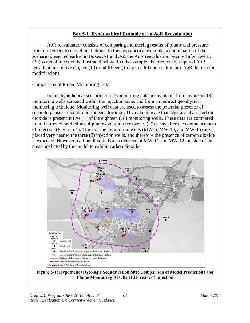
Draft UIC Program Class VI Well Area of 61 March 2011 Review Evaluation and Corrective Action Guidance
Box 5-1. Hypothethical Example of an AoR Reevaluation
AoR reevaluation consists of comparing monitoring results of plume and pressure front movement to model predictions. In this hypothetical example, a continuation of the scenario presented earlier in Boxes 3-1 and 3-2, the AoR reevaluation required after twenty (20) years of injection is illustrated below. In this example, the previously required AoR reevaluations at five (5), ten (10), and fifteen (15) years did not result in any AoR delineation modifications.
Comparison of Plume Monitoring Data
In this hypothetical scenario, direct monitoring data are available from eighteen (18)
monitoring wells screened within the injection zone, and from an indirect geophysical monitoring technique. Monitoring well data are used to assess the potential presence of separate-phase carbon dioxide at each location. The data indicate that separate-phase carbon dioxide is present at five (5) of the eighteen (18) monitoring wells. These data are compared to initial model predictions of plume evolution for twenty (20) years after the commencement of injection (Figure 5-1). Three of the monitoring wells (MW-5, MW-10, and MW-15) are placed very near to the three (3) injection wells, and therefore the presence of carbon dioxide is expected. However, carbon dioxide is also detected at MW-11 and MW-12, outside of the areas predicted by the model to exhibit carbon dioxide.
Figure 5-1: Hypothetical Geologic Sequestration Site: Comparison of Model Predictions and
Plume Monitoring Results at 20 Years of Injection
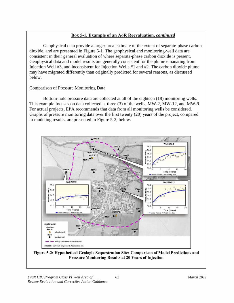
Draft UIC Program Class VI Well Area of 62 March 2011 Review Evaluation and Corrective Action Guidance
Box 5-1. Example of an AoR Reevaluation, continued
Geophysical data provide a larger-area estimate of the extent of separate-phase carbon dioxide, and are presented in Figure 5-1. The geophysical and monitoring-well data are consistent in their general evaluation of where separate-phase carbon dioxide is present. Geophysical data and model results are generally consistent for the plume emanating from Injection Well #3, and inconsistent for Injection Wells #1 and #2. The carbon dioxide plume may have migrated differently than originally predicted for several reasons, as discussed below.
Comparison of Pressure Monitoring Data
Bottom-hole pressure data are collected at all of the eighteen (18) monitoring wells.
This example focuses on data collected at three (3) of the wells, MW-2, MW-12, and MW-9. For actual projects, EPA recommends that data from all monitoring wells be considered. Graphs of pressure monitoring data over the first twenty (20) years of the project, compared to modeling results, are presented in Figure 5-2, below.
Figure 5-2: Hypothetical Geologic Sequestration Site: Comparison of Model Predictions and
Pressure Monitoring Results at 20 Years of Injection
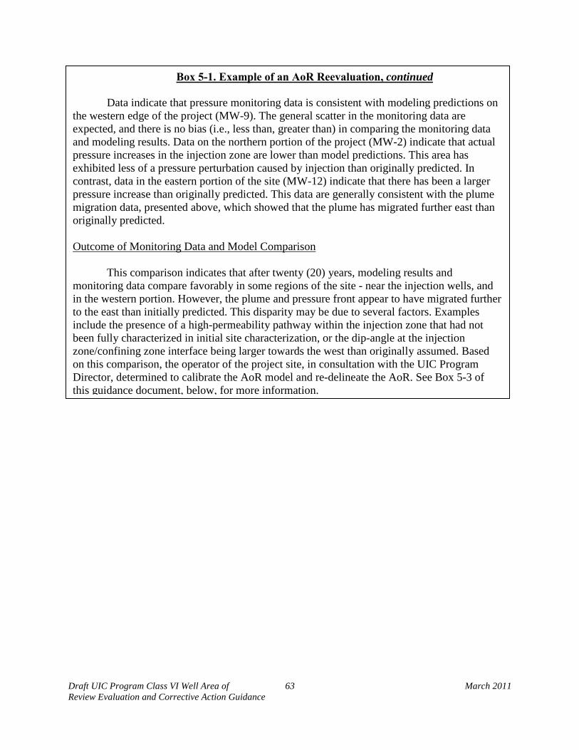
Draft UIC Program Class VI Well Area of 63 March 2011 Review Evaluation and Corrective Action Guidance
Box 5-1. Example of an AoR Reevaluation, continued
Data indicate that pressure monitoring data is consistent with modeling predictions on the western edge of the project (MW-9). The general scatter in the monitoring data are expected, and there is no bias (i.e., less than, greater than) in comparing the monitoring data and modeling results. Data on the northern portion of the project (MW-2) indicate that actual pressure increases in the injection zone are lower than model predictions. This area has exhibited less of a pressure perturbation caused by injection than originally predicted. In contrast, data in the eastern portion of the site (MW-12) indicate that there has been a larger pressure increase than originally predicted. This data are generally consistent with the plume migration data, presented above, which showed that the plume has migrated further east than originally predicted.
Outcome of Monitoring Data and Model Comparison
This comparison indicates that after twenty (20) years, modeling results and
monitoring data compare favorably in some regions of the site - near the injection wells, and in the western portion. However, the plume and pressure front appear to have migrated further to the east than initially predicted. This disparity may be due to several factors. Examples include the presence of a high-permeability pathway within the injection zone that had not been fully characterized in initial site characterization, or the dip-angle at the injection zone/confining zone interface being larger towards the west than originally assumed. Based on this comparison, the operator of the project site, in consultation with the UIC Program Director, determined to calibrate the AoR model and re-delineate the AoR. See Box 5-3 of this guidance document, below, for more information.
Draft UIC Program Class VI Well Area of 64 March 2011 Review Evaluation and Corrective Action Guidance
Box 5-2. Model Calibration Case Study: Frio Brine Pilot Project
Pilot projects of geologic sequestration can provide valuable insight into modeling predictions and monitoring results comparison. The Frio Brine Pilot Project, in Dayton, Texas, is an early experimental project conducted primarily by researchers at the Texas Bureau of Economic Geology and Lawrence Berkeley National Laboratory. Two carbon dioxide injection and monitoring experiments (Frio I and Frio II) have been conducted at Frio, and supplemented by numerical modeling. In this text-box, separate-phase carbon dioxide data from monitoring wells, pressure monitoring data, and geophysical monitoring data are presented. These figures and discussion are taken from Doughty et al. (2007) and Ajo-Franklin et al. (2008).
A geologic schematic of the Frio pilot site is shown in Figure 5-3. For the Frio I pilot, 1,600 metric tons of carbon dioxide were injected over 10 days into a steeply dipping brine-saturated later at a depth of 1,500 m. For the Frio II pilot, approximately 350 metric tons of carbon dioxide was injected at a depth of 1,600 m. A number of pre-injection site characterization, and operational and post-injection monitoring activities were conducted along with both injections.
Figure 5-3: Geologic Schematic of Frio Brine Pilot Project. The arrow at top indicates the north
direction (from Doughty et al., 2007). Reproduced with kind permission of Springer Science + Business Media.
For the Frio-I pilot, a numerical model was calibrated by constraining the value of
several parameters to a variety of monitoring data. Key calibration targets were determined to be multi-phase flow parameters that describe the relative permeability-saturation relationship,
Frio I Injection
Frio II Injection
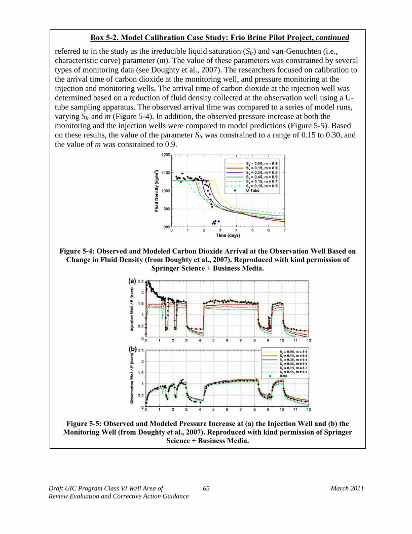
Draft UIC Program Class VI Well Area of 65 March 2011 Review Evaluation and Corrective Action Guidance
Box 5-2. Model Calibration Case Study: Frio Brine Pilot Project, continued
referred to in the study as the irreducible liquid saturation (Slr) and van-Genuchten (i.e., characteristic curve) parameter (m). The value of these parameters was constrained by several types of monitoring data (see Doughty et al., 2007). The researchers focused on calibration to the arrival time of carbon dioxide at the monitoring well, and pressure monitoring at the injection and monitoring wells. The arrival time of carbon dioxide at the injection well was determined based on a reduction of fluid density collected at the observation well using a U-tube sampling apparatus. The observed arrival time was compared to a series of model runs, varying Slr and m (Figure 5-4). In addition, the observed pressure increase at both the monitoring and the injection wells were compared to model predictions (Figure 5-5). Based on these results, the value of the parameter Slr was constrained to a range of 0.15 to 0.30, and the value of m was constrained to 0.9.
Figure 5-4: Observed and Modeled Carbon Dioxide Arrival at the Observation Well Based on
Change in Fluid Density (from Doughty et al., 2007). Reproduced with kind permission of Springer Science + Business Media.
Figure 5-5: Observed and Modeled Pressure Increase at (a) the Injection Well and (b) the
Monitoring Well (from Doughty et al., 2007). Reproduced with kind permission of Springer Science + Business Media.
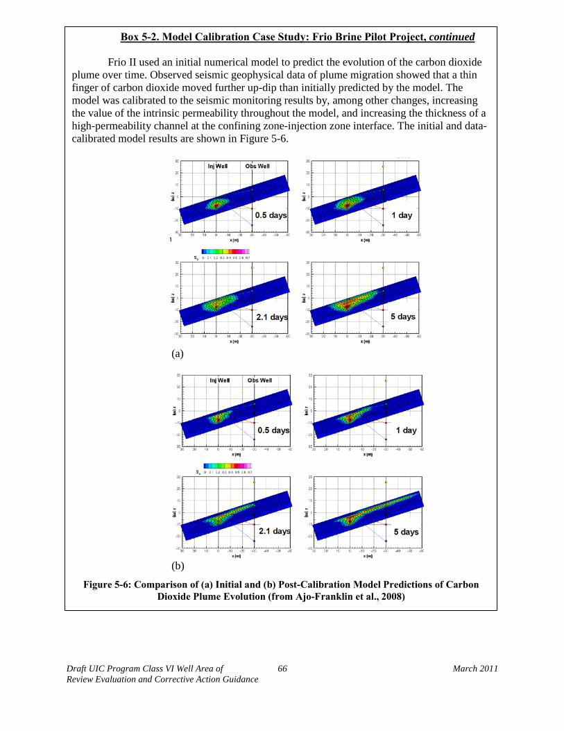
Draft UIC Program Class VI Well Area of 66 March 2011 Review Evaluation and Corrective Action Guidance
Box 5-2. Model Calibration Case Study: Frio Brine Pilot Project, continued Frio II used an initial numerical model to predict the evolution of the carbon dioxide
plume over time. Observed seismic geophysical data of plume migration showed that a thin finger of carbon dioxide moved further up-dip than initially predicted by the model. The model was calibrated to the seismic monitoring results by, among other changes, increasing the value of the intrinsic permeability throughout the model, and increasing the thickness of a high-permeability channel at the confining zone-injection zone interface. The initial and data-calibrated model results are shown in Figure 5-6.
(a)
(b)
Figure 5-6: Comparison of (a) Initial and (b) Post-Calibration Model Predictions of Carbon Dioxide Plume Evolution (from Ajo-Franklin et al., 2008)

Draft UIC Program Class VI Well Area of 67 March 2011 Review Evaluation and Corrective Action Guidance
EPA recommends that the Class VI injection well owner(s) or operator(s) submit any new operational, monitoring, or site characterization data that have been received since the last AoR reevaluation to the UIC Program Director. EPA also recommends that details regarding how this information has been incorporated into the site computational model be presented, as newly received operational or site characterization data may impact model input parameter values.
Integral to demonstrating that the current AoR delineation is adequate is the comparison of monitoring data and model predictions. EPA recommends that this comparison take the form of graphics and informative maps showing general agreement between monitored data and model predictions, and that all available monitoring data be considered, including fluid geochemistry monitoring, pressure monitoring, and geophysical surveys.
5.2.2. Modifying the Existing AoR Delineation
Any significant difference between operational monitoring results and the existing model predictions that are the basis for the AoR delineation, for example as discussed in Section 5.1.3 of this guidance document, above, warrants a modification to the existing AoR delineation [§146.84(e)]. The steps in revision of the AoR delineation include adjusting the site conceptual model, adjusting model parameters (i.e., model calibration), and presentation of adjusted model results and the newly delineated AoR to the UIC Program Director.
5.2.2.1. Adjusting Site Conceptual Model
EPA recommends that the site conceptual model be revised based on new site characterization, operational, and in some cases, new monitoring data. The new conceptual site model schematic may be provided to the UIC Program Director along with the AoR reevaluation information, with any changes highlighted. Examples of changes to the conceptual model include new injection wells, newly elucidated geologic features (i.e., stratigraphic layers), or a revised permeability field.
5.2.2.2. Model Calibration
Model calibration consists of adjusting relevant model parameters to reduce differences between model results and new monitoring data. The term ‘calibration targets’ refers to the monitoring data results used to adjust the computational model. Examples of calibration targets include carbon dioxide saturation values, or fluid pressures. Calibration may include incorporating additional heterogeneities or highly-permeable pathways. In general, EPA recommends that model calibration focuses on a minimum number of the most significant parameters, and avoids optimizing strongly correlated parameters. Intrinsic permeability of the formation and relative permeability-saturation function parameters, are likely of significant influence on modeling results but are subject to significant uncertainty A case study of model calibration to monitoring data at an early GS research site, the Frio Brine Pilot in Texas, is provided in Box 5-2 of this guidance document, above.
Model parameters may be adjusted using an objective function, and/or adjusted ‘manually’ based on best professional judgment. Any model parameters adjusted during calibration are
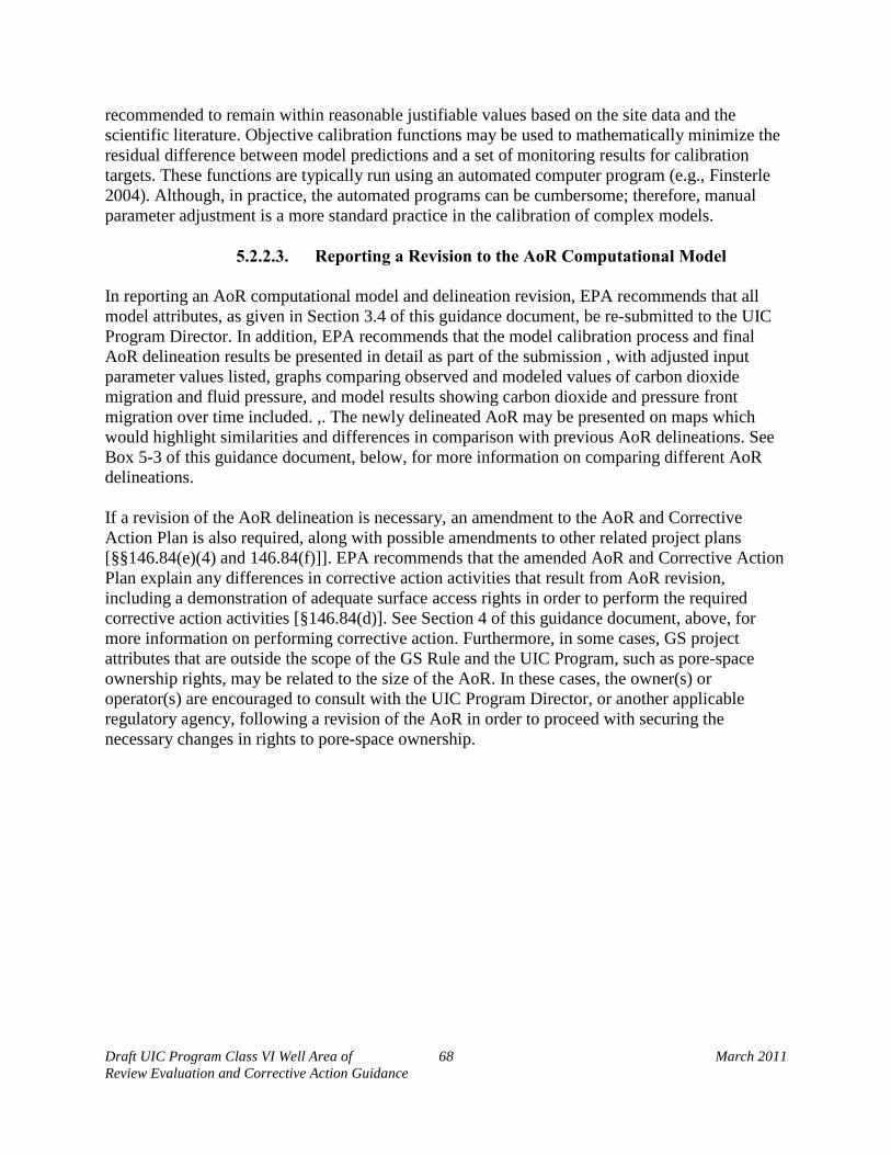
Draft UIC Program Class VI Well Area of 68 March 2011 Review Evaluation and Corrective Action Guidance
recommended to remain within reasonable justifiable values based on the site data and the scientific literature. Objective calibration functions may be used to mathematically minimize the residual difference between model predictions and a set of monitoring results for calibration targets. These functions are typically run using an automated computer program (e.g., Finsterle 2004). Although, in practice, the automated programs can be cumbersome; therefore, manual parameter adjustment is a more standard practice in the calibration of complex models.
5.2.2.3. Reporting a Revision to the AoR Computational Model
In reporting an AoR computational model and delineation revision, EPA recommends that all model attributes, as given in Section 3.4 of this guidance document, be re-submitted to the UIC Program Director. In addition, EPA recommends that the model calibration process and final AoR delineation results be presented in detail as part of the submission , with adjusted input parameter values listed, graphs comparing observed and modeled values of carbon dioxide migration and fluid pressure, and model results showing carbon dioxide and pressure front migration over time included. ,. The newly delineated AoR may be presented on maps which would highlight similarities and differences in comparison with previous AoR delineations. See Box 5-3 of this guidance document, below, for more information on comparing different AoR delineations. If a revision of the AoR delineation is necessary, an amendment to the AoR and Corrective Action Plan is also required, along with possible amendments to other related project plans [§§146.84(e)(4) and 146.84(f)]]. EPA recommends that the amended AoR and Corrective Action Plan explain any differences in corrective action activities that result from AoR revision, including a demonstration of adequate surface access rights in order to perform the required corrective action activities [§146.84(d)]. See Section 4 of this guidance document, above, for more information on performing corrective action. Furthermore, in some cases, GS project attributes that are outside the scope of the GS Rule and the UIC Program, such as pore-space ownership rights, may be related to the size of the AoR. In these cases, the owner(s) or operator(s) are encouraged to consult with the UIC Program Director, or another applicable regulatory agency, following a revision of the AoR in order to proceed with securing the necessary changes in rights to pore-space ownership.
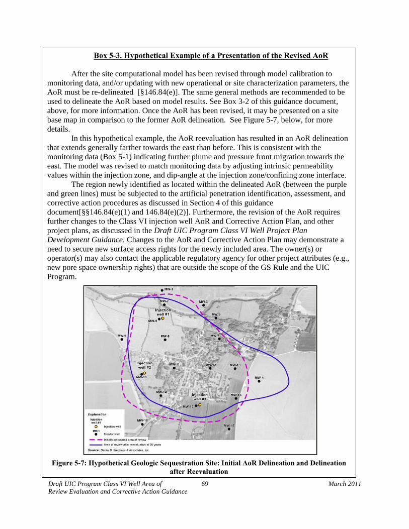
Draft UIC Program Class VI Well Area of 69 March 2011 Review Evaluation and Corrective Action Guidance
Box 5-3. Hypothetical Example of a Presentation of the Revised AoR
After the site computational model has been revised through model calibration to monitoring data, and/or updating with new operational or site characterization parameters, the AoR must be re-delineated [§146.84(e)]. The same general methods are recommended to be used to delineate the AoR based on model results. See Box 3-2 of this guidance document, above, for more information. Once the AoR has been revised, it may be presented on a site base map in comparison to the former AoR delineation. See Figure 5-7, below, for more details.
In this hypothetical example, the AoR reevaluation has resulted in an AoR delineation that extends generally farther towards the east than before. This is consistent with the monitoring data (Box 5-1) indicating further plume and pressure front migration towards the east. The model was revised to match monitoring data by adjusting intrinsic permeability values within the injection zone, and dip-angle at the injection zone/confining zone interface.
The region newly identified as located within the delineated AoR (between the purple and green lines) must be subjected to the artificial penetration identification, assessment, and corrective action procedures as discussed in Section 4 of this guidance document[§§146.84(e)(1) and 146.84(e)(2)]. Furthermore, the revision of the AoR requires further changes to the Class VI injection well AoR and Corrective Action Plan, and other project plans, as discussed in the Draft UIC Program Class VI Well Project Plan Development Guidance. Changes to the AoR and Corrective Action Plan may demonstrate a need to secure new surface access rights for the newly included area. The owner(s) or operator(s) may also contact the applicable regulatory agency for other project attributes (e.g., new pore space ownership rights) that are outside the scope of the GS Rule and the UIC Program.
Figure 5-7: Hypothetical Geologic Sequestration Site: Initial AoR Delineation and Delineation
after Reevaluation
Draft UIC Program Class VI Well Area of 70 March 2011 Review Evaluation and Corrective Action Guidance
References Ajo-Franklin, J., C. Doughty, and T.M. Daley. Combining Analysis of Continuous Active-
Source Seismic Monitoring (CASSM) and Multiphase Flow Modeling for CO2
Sequestration: The Frio II Brine Pilot. Presented at the 7th Annual Conference on Carbon Capture and Sequestration May 5-8: Pittsburg, Pennsylvania.
ASTM, 2005. Standard guide for locating abandoned wells. Designation D 6285-99 (Reapproved 2005).
Bachu, S. and B. Bennion. 2008. Effects of in-situ conditions on relative permeability
characteristics of CO2
-brine systems. Environ Geology, 54:1707-1722.
Carle, S.F. 1999. T-PROGS: Transition Probability Geostatistical Software, Version 2.1. Celia, M. A. and J.M. Nordbotten. 2009. Practical modeling approaches for geologic storage of
carbon dioxide. Ground Water, 47:627-638. Close, D., D. Cho, F. Horn, and H. Edmundson. 2009. The Sound of Sonic: A Historical
Perspective and Introduction to Acoustic Logging. CSEG Recorder pp. 34-43 Doughty, C. and K. Pruess. 2004. Modeling supercritical carbon dioxide injection in
heterogeneous porous media, Vadose Zone Journal, 3(3):837–847. Doughty, C. 2007. Modeling geologic storage of carbon dioxide: Comparison of non-hysteretic
and hysteretic characteristic curves. Energy Conversion and Management 48: 1768–1781. Doughty, C., B.M. Freifeld, and R.C. Trautz, 2007, Site characterization for CO2
geologic storage and vice versa – the Frio brine pilot, Texas, USA as a case study, Environmental Geology, DOI 10.10007/s00254-007-0942-0.
Duguid, A., and W. Crow. 2007. CO2
Well Integrity and Wellbore Monitoring. Presented at the Carbon Sequestration Leadership Forum (CSLF) 2nd Capacity Building in Emerging Economies Workshop, 18-19 October 2007, Porto Alegre, Brazil.
Fetter, C.W. 2001. Applied Hydrogeology, 4th
Edition. Prentice Hall, Upper Saddle River, NJ. 598p.
Finsterle, S. 2004. Mulitphase inverse modeling: Review and iTOUGH2 applications. Vadose Zone Journal, 3:747-762.
Flett M., R. Gurton, and G. Weir. 2007. Heterogeneous saline formations for carbon dioxide
disposal: Impact of varying heterogeneity on containment and trapping. J. Petroleum Science and Engineering, 57:106-118.
Draft UIC Program Class VI Well Area of 71 March 2011 Review Evaluation and Corrective Action Guidance
Friskchknecht, F.C., P.V. Raab, and J.J. van Ee. 1985. Project Summary: Location of abandoned wells with geophysical methods. EPA-600/SR-84-085.
Gerritsen, M.G. and L.J. Durlofsky. 2005. Modeling fluid flow in oil reservoirs. Annual Reviews
in Fluid Mechanics, 37:211-238. Green, D.W. and R.H. Perry. 2008. Perry's Chemical Engineers' Handbook, 8th Edition.
McGraw-Hill. Gochioco, L.M. and F. Ruev Jr. 2006. Detecting and imaging hard-to-find abandoned wells and
pipelines. The Leading Edge, March 2006, 358-361. Han, W.S. and B. McPherson, 2008. Comparison of two equations of state for application of
carbon dioxide sequestration. Advances in Water Resources, 31:877-890. Ide, T., S.J. Friedmann, and H. Herzog. 2006. Carbon Dioxide Leakage through Existing Wells:
Current Technology and Regulations," presented at the 8th International Conference on Greenhouse Gas Control Technologies, Trondheim, Norway, June (2006).
Izgec, O., B. Demiral, H. Bertlin, and S. Arkin. 2008. CO2
injection into saline carbonate aquifer formations II: Comparison of numerical simulations to experiments. Transport in Porous Media, 73: 57-74.
Jordan, P.W. and J.L. Hare. 2002. Locating Abandoned Wells: A Comprehensive Manual of Methods and Resources. Prepared for Solution Mining Research Institute, Research Project Report No. 2002-SMRI.
Juanes, R., E.J. Spiteri, F.M. Orr Jr., and M.J. Blunt. 2006. Impact of relative permeability
hysteresis on geological CO2
storage. Water Resources Research, 42. W12418.
Knauss K.G., J.W. Johnson, and C.I. Steefel. 2005. Evaluation of the impact of CO2, co-contaminant gas, aqueous fluid and reservoir rock interactions on the geologic sequestration of CO2
. Chemical Geology, 217:339-350.
Law, D.H.-S. and S. Bachu. 1996. Hydrogeological and numerical analysis of CO2
disposal in deep aquifers in the Alberta sedimentary basin. Energy Conversion and Management, 37:1167-1174.
Lindeberg, E. 1997. Escape of CO2
from aquifers. Energy Conversion and Management, 38:S235-S240.
Miller, C.T., G. Christakos, P.T. Imhoff, J.F. McBride, J.A. Pedit, and J.A. Trangenstein. 1998. Mulitphase flow and transport modeling in heterogeneous porous media: challenges and approaches. Advances in Water Resources, 21(2): 77-120.
Draft UIC Program Class VI Well Area of 72 March 2011 Review Evaluation and Corrective Action Guidance
Nordbotten, J.M., M.A. Celia, and S. Bachu. 2005. Injection and storage of CO2 in deep saline aquifers: Analytical solution for CO2
plume evolution during injection. Transport in Porous Media 58:339–360.
National Research Council (NRC). 2007. Models in Environmental Regulatory Decision Making. Prepared by Committee on Models in the Regulatory Decision Process.
Obi, E.-O. I., and M.J. Blunt, 2006. Streamline-based simulation of carbon dioxide storage in a
North Sea aquifer. Water Resources Research, 42: W03414. Perrin, J.-C., M. Krause, and S. M. Benson. 2008. Relative permeability properties of the
CO2
/Brine system in saline aquifers: An experimental study. Presented at the Seventh Annual Conference on Carbon Capture and Sequestration, Pittsburgh Pennsylvania.
Perry, R.H. and D. Green. 1984. Perry’s Chemical Engineers’ Handbook, Sixth Edition. McGraw-Hill Book Co., New York NY.
Plug, W.J. and J. Bruining. 2007. Capillary pressure for the sand- CO2-water system under
various pressure conditions. Application to CO2
sequestration. Advances in Water Resources. 30: 2339-2353.
Pruess, K. and N. Spycher. 2007. ECO2N – A fluid property module for the TOUGH2 code for studies of CO2
storage in saline aquifers. Energy Conversion and Management. Vol 48, 1761-1767.
Pruess K, J. Garcia, T. Kovscek, T. C. Oldenburg, J. Rutqvist, C. Steefel and T. Xu. 2004. Code intercomparison builds confidence in numerical simulation models for geologic disposal of CO2
.
Pruess, K. 2008. Leakage of CO2
from geologic storage: Role of secondary accumulation at shallow depth. International Journal of Greenhouse Gas Control, 2: 37-46.
Randhol, P., K. Valencia, A. Taghipour, I. Akervoll and I.M. Carlsen. 2007. Ensuring Well Integrity in Connection with CO2
Injection. SINTEF report 31.6920.00/02/07.
Reynolds, R.R., and R.D. Kiker, 2003, Produced Water and Associated Issues — A Manual for the Independent Operator. Oklahoma Geological Survey Open File Report 6-2003. Prepared for the South Midcontinent Region of the Petroleum Technology Transfer Council.
Rutqvst, J., J.T. Birkholzer, and C. –F Tsang, 2008. Coupled Reservoir-Geomechanical Analysis
of the Potential for Tensile and Shear Failure Associated with CO2
Injection in Multilayered Reservoir Caprock Systems, International Journal of Rock Mechanics and Mining Sciences, 45(2), pp. 132-143.
Draft UIC Program Class VI Well Area of 73 March 2011 Review Evaluation and Corrective Action Guidance
Saripalli, P., and P. McGrail. 2002. Semi-analytical approaches to modeling deep well injection of CO2
for geologic sequestration. Energy Conversion and Management, 43: 185-198.
Schnaar, G., and D. C. Digiulio. 2009. Computational modeling of the geologic sequestration of carbon dioxide. Vadose Zone Journal, 8:389-403.
Spycher, N., K. Pruess, and J. Ennis-King. 2003. Carbon dioxide-water mixtures in geologic
sequestration of carbon dioxide. I. Assessment and calculation of mutual solubilities from 12 to 100 degrees Celsius and up to 600 bar. Geochemical et Cosmochimica Acta, 67:3015-3031.
Spycher, N., and K. Pruess. 2005. Carbon dioxide-water mixtures in geologic sequestration of
carbon dioxide. II. Partitioning in chloride brines at 12-100 degrees Celsius and up to 600 bar. Geochemical et Cosmochimica Acta, 69:3309-3320.
Stone, H.L. 1970. Probability model for estimating three-phase relative permeability. Trans.
AIME 249, 214-218. Tamimi, A. E., B. Rinker, and O. C. Sandall. 1994. Diffusion coefficients for hydrogen sulfide,
carbon dioxide, and nitrous oxide in water over the temperature range 293-368 K. J. Chem. Eng. Data, 39: 330-332.
Thornhill, J.T., T.E. Short, and L. Silka. 1982. Application of the Area of Review Concept.
Ground Water, Vol. 20, 32-38. United States Environmental Protection Agency (US EPA). 2002. Drinking Water Academy,
Underground Injection Control Modules, Lesson 8: Area of Review (http://www.epa.gov/safewater/dwa/pdfs/2%20uic%20modules/dwaUIC-uicpermit2.pdf)
US EPA. 2003. Draft Guidance on the Development, Evaluation, and Application of Regulatory
Environmental Models. Prepared by The Council for Regulatory Environmental Modeling.
United States Geological Survey (USGS). 1995. Fact Sheet 163-95: Magnetic Surveys for
Locating Abandoned Wells. Watson, T.L. 2009. CO2 Storage: Wellbore Integrity Evaluation and Integrity Across the
Caprock. Presented at the 2009 SPE Conference on CO2
Capture, 2-4 November 2009, San Diego, California.
Xu, T., E. Sonnenthal, N. Spycher, and K. Pruess. 2006. TOUGHREACT—A simulation program for non-isothermal multiphase reactive geochemical transport in variably saturation geologic media: Applications to geothermal injectivity and CO2
geological sequestration. Computers & Geosciences, 32:145-165.

Draft UIC Program Class VI Well Area of 74 March 2011 Review Evaluation and Corrective Action Guidance
Xu, T., J.A. Apps, K. Pruess, and H. Yamamoto. 2007. Numerical modeling of injection and mineral trapping of CO2 with H2S and SO2
in a sandstone formation. Chemical Geology, 242:319-346.
Zhang, K., C. Doughty, Y.-S. Wu, and K. Pruess. 2007. Efficient parallel simulation of CO2
geologic sequestration in saline aquifers, SPE 106026, presented at 2007 SPE Reservoir Simulation Symposium, Houston, TX, February 26-28.
Zhou, Q., J.T. Birkholzer, C.-F Tsang, and J. Rutqvist. 2008. A method for quick assessment of CO2
storage capacity in closed and semi-closed saline formations. International Journal of Greenhouse Gas Control (In Press).
Zhou, W., M.J. Stenhouse, R. Arthur, S. Whittaker, D.H.-S. Law, R. Chalaturnyk, and W. Jazrawi. 2004. The IEA Weyburn CO2 monitoring and storage project – modeling of the long-term migration of CO2 from Weyburn. In: Wilson M., J. Gale, E.S. Rubin, D.W. Keith, C.F. Gilboy, T. Morris, and K. Thambimuthu (Eds) Greenhouse gas control technologies: proceedings of the 7th International Conference on Greenhouse Gas Control Technologies, 5-9 Sept. 2004, Vancouver, Canada.