SDT 233

EXPORT DIVERSIFICATION AND GROWTH IN EMERGING ECONOMIES

Autor: Manuel R. Agosin

Santiago, Mar. 2007

Serie Documentos de Trabajo

N 233

EXPORT DIVERSIFICATION AND GROWTH IN EMERGING ECONOMIES 1

Manuel R. Agosin Departamento de Economía

Universidad de Chile

Resumen

This paper develops and tests a model of growth in that emphasizes the introduction of new export as the main source of growth in countries that are far within the world technological frontier and that depend for growth on adapting existing products to their economic environment. It seeks to capture the stylized facts behind growth in countries as different as Korea, Taiwan, Mauritius, Finland, China, and Chile, all of which have depended on export diversification for their growth. Thus the widening of comparative advantage is seen as the main force behind economic growth. The hypothesis of export diversification is tested with an empirical growth model. Controlling for other variables that affect growth, export diversification, alone and interacted with per capital export volume growth, is found to be highly significant in explaining per capita GDP growth over the 1980-2003 period.

Palabras Claves:

Growth, export.

1 I am grateful for the able research assistance of Alfie Ulloa and Alejandro Támola. I acknowledge the useful comments made by Robert Devlin and Roberto Bouzas. Ricardo Ffrench-Davis read the manuscript thoroughly and made suggestions that improved it significantly.

Export Diversification and Growth in Emerging Economies

Manuel R. Agosin* Department of Economics, Universidad de Chile

Address: Diagonal Paraguay 257, Room 1505, Santiago Chile Phone: +56 (2) 978-3428; cell: +56 (9) 8245-1520

Email: managosin@econ.uchile.cl; webpage: www.econ.uchile.cl

Summary:

This paper develops and tests a model of growth in that emphasizes the introduction of new

export as the main source of growth in countries that are far within the world technological

frontier and that depend for growth on adapting existing products to their economic environment.

It seeks to capture the stylized facts behind growth in countries as different as Korea, Taiwan,

Mauritius, Finland, China, and Chile, all of which have depended on export diversification for

their growth. Thus the widening of comparative advantage is seen as the main force behind

economic growth. The hypothesis of export diversification is tested with an empirical growth

model. Controlling for other variables that affect growth, export diversification, alone and

interacted with per capital export volume growth, is found to be highly significant in explaining

per capita GDP growth over the 1980-2003 period.

Key words: Comparative perspectives on economic growth; export diversification; trade; Asia,

Latin America

* I am grateful for the able research assistance of Alfie Ulloa and Alejandro Támola. A first version of this paper was presented at a conference on Growth and Equity held in CEPAL, Santiago, on September 2, 2005. I acknowledge the useful comments made by Robert Devlin and Roberto Bouzas. Ricardo Ffrench-Davis read the manuscript thoroughly and made suggestions that improved it significantly. I am also thankful to my colleagues in the Department of Economics, who made good suggestions for improvement during a presentation to the Department’s weekly seminar series.

2

Introduction

This paper explores the connection between export expansion and GDP growth, with

reference to the diverging growth experience of East Asian and Latin American countries (LAC).

We are interested in the issue of whether export growth is associated with overall economic

growth. In a statistical sense, the relation must hold, since exports are a part of GDP. Here the

focus will be on whether there is a particular kind of export growth which can result in sustained

growth both in exports and GDP. We posit that countries with diversified export structures are

able to record consistently higher export growth than countries where exports are concentrated in

a few products.

Section I presents some analytical considerations of why output and export

diversification (OED) should be positive for growth. In section II, a model is developed

capturing the stylized facts of an economy where growth occurs through adaptation of foreign

goods rather than through genuine innovation. After looking at the export and growth experience

for Latin America and Asia (section III), we show the plausibility of a negative association

between export concentration and growth operating through the effect of concentration on export

and output volatility (section IV). Then, in section V, we show that an export diversification

index and export growth interacted with the diversification index (a sort of diversification-

weighted export growth rate) are strong explanatory variables in a simple empirical growth

model estimated with cross section data for 1980-2003. The coefficients yielded by the empirical

model are used, in section VI, to estimate the average contribution of export diversification,

investment, and the rule of law to growth in LAC and Asian countries. Section VI recapitulates.

3

I. Analytical considerations

Why would export diversification be beneficial for growth? There are potentially two

different types of effects. The first is what we call the portfolio effect, which takes its name from

the finance literature. The greater the degree of diversification the less volatile will be export

earnings. Less volatile exports are associated with lower variance of GDP growth. This is, in

itself, a positive aspect of diversification, since countries with imperfect (or no) access to world

financial markets will not be able to smooth consumption in the face of large fluctuations in

exports and output.

In addition, the variance and the mean of the growth rate may be negatively correlated for

other reasons. This adverse effect of volatility on average growth could result from hysteresis.

Periods of contraction lead to the destruction of installed capacity and to deskilling of the labor

force, both of which cannot be easily undone during the next boom. Also, countries whose

exports are highly dependent on one or a few products tend to have more volatile real exchange

rates than countries with diversified export structures, and real exchange rate volatility

discourages investment in tradable goods or services.

Second, there is the dynamic effect of export diversification. Long run growth is

associated with learning to produce an expanding range of goods. This view sees growth as being

the result of adding new products to the export and production basket. In countries that have few

indigenous sources of productivity growth, most of their productivity advances come from the

investment process itself, as new capital goods embody productivity change and the opening up

of new sectors that have higher factor productivity than existing sectors. These sectors are not

4

new to the world, since they are produced elsewhere. But they are new to the economy where

they are being introduced and represent technical change.

One of the single most important characteristics of countries with low per capita income

is the fact that they have a comparative advantage in a very limited range of goods. In other

words, because of the paucity of skills or lack of complementary inputs (some non-traded), these

countries are unable to apply knowledge about production that exists elsewhere in the world. As

a country develops, it becomes increasingly able to produce an ever wider range of goods and

can begin to compete in international markets in them. Therefore, there is a line of causation that

runs from income per capita to diversification of production and exports. While not the only one,

the ability to export certainly can be judged to be an appropriate indicator of international

competitiveness.

But there may be a causal relationship running from efforts to diversify exports to growth

as well. The acquisition of new comparative advantages may be a powerful encouragement to

more rapid economic growth. In other words, countries whose comparative advantages remain

confined to a narrow range of low-technology goods grow slowly, and countries that are able to

broaden their comparative advantages grow more rapidly. This is the major hypothesis of this

paper.

Production of goods that represent a step up the technological ladder for a country require

trained labor, but the introduction of such goods also speed up the training of workers, as those

employed in the new ventures tend to train others. In addition, the introduction of a new type of

production increases the likelihood that other new sectors will arise, as human capital employed

in the new sector may come up with new production ideas.

5

In a recent literature, it has been argued convincingly that producers do not have

complete knowledge of the comparative advantages of their economies. There are elements of

comparative advantage that are, so to speak, discovered in the process of producing a new good.

According to this view, introducing a new good to the export basket has an externality, because it

reveals to other producers the underlying structure of the economy’s costs. However, in a

developing country context, the introduction of a new good or the application of a new

technology is easily copied, because such technological innovations (for the economy where it is

being introduced) cannot be patented. Therefore, the leader will not reap all the benefits of his

investment (see Hausmann and Rodrik, 2003).

Another similar strand emphasizes the discovery of foreign demand (Vettas, 2000).

Producing a new product for export markets may reveal to domestic producers that there is

demand in international markets for products that can be (or are being) produced domestically.1

In fact, the introduction of a new good may create demand abroad for that good by making

consumers aware of its existence and characteristics. Like cost discoveries, demand discoveries

represent non-patentable innovations, which, as such, can be easily imitated. Again, there is here

an important externality that can lead to a sustained spurt of growth.

A further development in the literature shows that producing a new export can have

additional growth-enhancing effects. Export discoveries are not random, but follow some

sequence. Countries that become good at producing a particular export are likely to develop

comparative advantages in related sectors. It has been observed that new exports cluster together

or follow a pattern in time (TV sets and DVDs or cell phones in China; different varieties of fruit

in Chile; different kinds of apparel in East Asia or Central America). This phenomenon can be

1 A case in point is wine in Chile. While wine had been produced since the 17th century, it was not until the mid 1980s that exports took off, mainly due to the fact that a few entrepreneurs discovered that, with some modifications of production techniques, Chilean wine could be sold very profitably in Europe (Agosin and Bravo-Ortega, 2007).

6

explained by observing that clusters of goods tend to utilize the same or similar public goods

(specific public institutions) and non-tradable inputs (roads, logistic services). Hence an export

discovery may facilitate the emergence of other new exports in the same or in closely related

sectors. This being the case, an export discovery has not only positive intra-industry growth

effects but also inter-industry spillovers (Hausmann and Klinger, 2007; Hausmann and Rodrik,

2006).

These hypotheses suggest that, indeed, export diversification should be associated with

economic growth, with export diversification the cause and economic growth the effect.

II. A model linking OED and growth

The purpose of this model is to attempt to capture these stylized facts. In a sense, it seeks

to put some flesh into the classic view of development as the result of the “advantages of

backwardness” (Gerschenkron, 1962). In other words, technologically backward economies can

grow at fast rates simply by copying what already exists elsewhere and don’t have to grow by

pushing out the technological frontier.2 Some countries, either due to policies or because

institutional arrangements are favorable, are able to reap the advantage of being inside the

technological frontier; others are not. Introducing goods that exist elsewhere constitutes an

innovation, however, that can be easily copied. It is precisely this that provides the impetus to

fast economic growth. The inability to reap the benefits of discovery is also the key market

failure that needs to be dealt with if an economy of these characteristics is to grow.

There is no aggregate production function and no technical change other than the one that

is embodied in the introduction of new, more sophisticated goods. Aggregate output is the sum 2 This is why the calculation of total factor productivity in developing economies makes so little sense.

7

of the value of production of all goods produced in the economy. Let us begin with an economy

that produces one traditional good (say, “sugar”) with land and labor. Sugar is the numeraire of

our economy (its price is unity). The introduction of any new good is the product of an idea, in

the sense of “self-discovery” in Hausmann and Rodrik (2003); in order to be profitable, any new

idea requires the existence of sector-specific public goods (for short, call both of them

“infrastructure”).

This approach is designed to capture the notion that there are two obstacles to self-

discovery: the information externalities involved in investing to introduce a product into a

developing country environment, since pioneers will incur costs in obtaining information which

will then become public knowledge; and the coordination problem that arises because the

profitability of any new endeavor depends on the simultaneous existence of suppliers of non-

traded inputs and sector-specific public goods.3

Following Romer (1993), aggregate production is the sum of all goods produced. Let us

assume that factor endowment consists of land (T), unskilled labor (L), and an initial human

capital (H0). Sugar production uses land and labor but not human capital; all modern goods use

labor and human capital but not land. There is an unlimited supply of unskilled labor, in the

sense of Lewis (1954), so that we don’t have to worry about running up against labor scarcity,

and the wage is fixed at its subsistence level ( w ).

∑∑+=i

jijijijijijj

T BAHLGpLTFY ),;,(),( (1)

3 Some examples of these services and infrastructure requirements, which are the essence of the coordination problem are discussed below.

8

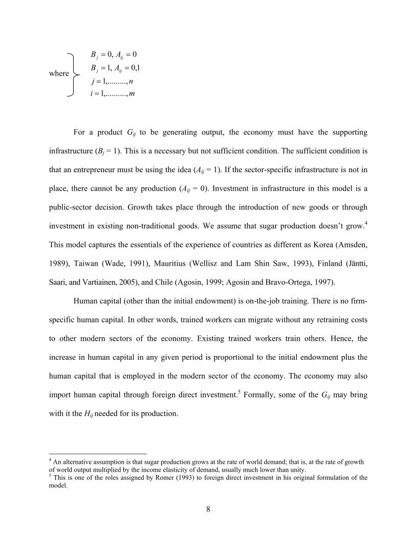
where

minj

AB

AB

ijj

ijj

.,,.........1,,.........1

1,0,1

0,0

==

==

==

For a product Gij to be generating output, the economy must have the supporting

infrastructure (Bj = 1). This is a necessary but not sufficient condition. The sufficient condition is

that an entrepreneur must be using the idea (Aij = 1). If the sector-specific infrastructure is not in

place, there cannot be any production (Aij = 0). Investment in infrastructure in this model is a

public-sector decision. Growth takes place through the introduction of new goods or through

investment in existing non-traditional goods. We assume that sugar production doesn’t grow.4

This model captures the essentials of the experience of countries as different as Korea (Amsden,

1989), Taiwan (Wade, 1991), Mauritius (Wellisz and Lam Shin Saw, 1993), Finland (Jäntti,

Saari, and Vartiainen, 2005), and Chile (Agosin, 1999; Agosin and Bravo-Ortega, 1997).

Human capital (other than the initial endowment) is on-the-job training. There is no firm-

specific human capital. In other words, trained workers can migrate without any retraining costs

to other modern sectors of the economy. Existing trained workers train others. Hence, the

increase in human capital in any given period is proportional to the initial endowment plus the

human capital that is employed in the modern sector of the economy. The economy may also

import human capital through foreign direct investment.5 Formally, some of the Gij may bring

with it the Hij needed for its production.

4 An alternative assumption is that sugar production grows at the rate of world demand; that is, at the rate of growth of world output multiplied by the income elasticity of demand, usually much lower than unity. 5 This is one of the roles assigned by Romer (1993) to foreign direct investment in his original formulation of the model.

9

)( 0 ∑∑+=j i

ijHHH μ& (2)

New ideas are the key to growth in this economy. Because many new ideas are variations

on existing ideas, new ideas (and new production sectors) are a function of the number of ideas

that are being exploited in the economy (Anm) and on the stock of human capital.

⎟⎟⎠

⎞⎜⎜⎝

⎛+= ∑∑

iij

jnm HHAJA 0;& (3)

The public sector builds sector-specific infrastructure that enables the introduction of new

ideas. We make the following assumptions: (1) the public sector balances its budget; (2) all

revenues come from taxing profits generated both in the modern sectors and in sugar production;

(3) government expenditures are either on investments in new infrastructure projects or in

consumption (CG), and (4) the cost of each infrastructure project is the same (and equal to λ).

From the condition of public-sector budget balance, we can obtain the number of new

infrastructure projects undertaken:

λππλτ /)/( Gj i

ijs CB −⎟⎟⎠

⎞⎜⎜⎝

⎛+= ∑∑& (4)

In this model, new infrastructure projects generate growth. However, since they must be

financed by tax revenue and the tax rate decreases the net profits of enterprises in the modern

sector, there is a trade-off between new infrastructure projects and investment by existing firms

10

in the modern sector, since investment is financed from retained earnings.6 We assume that in the

modern sector after-tax profits are fully reinvested in existing ventures. After-tax profits in sugar

are consumed.

When will a new product be introduced into the economy? Assume that a prospective

entrepreneur borrows C0 in period 0 to gather information about introducing a new idea into the

economy. She also knows that she needs a capital of C1 to make the project operational. This she

will borrow in period 1 if and only if the project indeed turns out to be profitable after the

requisite information has been obtained. The project yields a profit of πij in period 2. But, in

period 1, the information that is needed to make sure the project is profitable becomes known to

all potential entrepreneurs.7

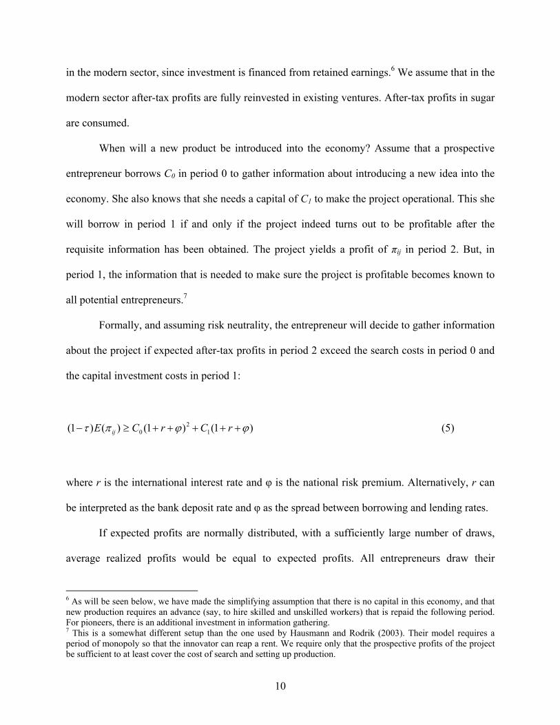
Formally, and assuming risk neutrality, the entrepreneur will decide to gather information

about the project if expected after-tax profits in period 2 exceed the search costs in period 0 and

the capital investment costs in period 1:

)1()1()()1( 12

0 ϕϕπτ +++++≥− rCrCE ij (5)

where r is the international interest rate and φ is the national risk premium. Alternatively, r can

be interpreted as the bank deposit rate and φ as the spread between borrowing and lending rates.

If expected profits are normally distributed, with a sufficiently large number of draws,

average realized profits would be equal to expected profits. All entrepreneurs draw their

6 As will be seen below, we have made the simplifying assumption that there is no capital in this economy, and that new production requires an advance (say, to hire skilled and unskilled workers) that is repaid the following period. For pioneers, there is an additional investment in information gathering. 7 This is a somewhat different setup than the one used by Hausmann and Rodrik (2003). Their model requires a period of monopoly so that the innovator can reap a rent. We require only that the prospective profits of the project be sufficient to at least cover the cost of search and setting up production.

11

information from the same pool. Some will wind up with profits that satisfy (5) and some will

not.

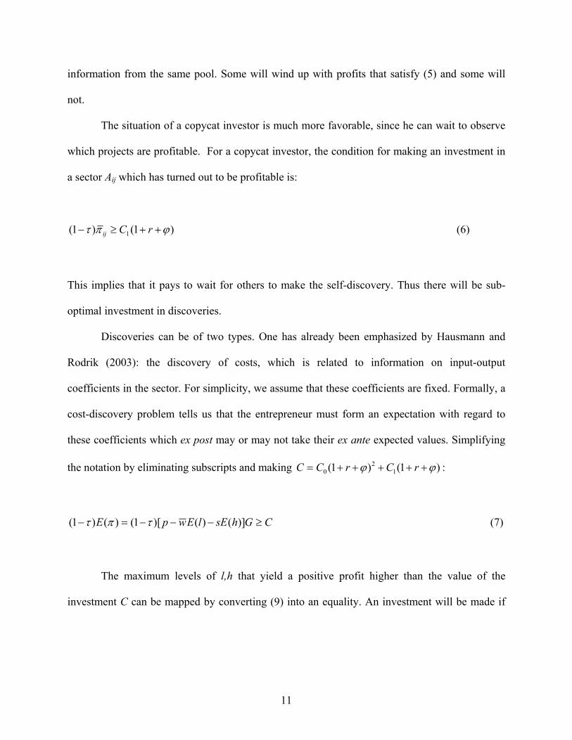
The situation of a copycat investor is much more favorable, since he can wait to observe

which projects are profitable. For a copycat investor, the condition for making an investment in

a sector Aij which has turned out to be profitable is:

)1()1( 1 ϕπτ ++≥− rCij (6)

This implies that it pays to wait for others to make the self-discovery. Thus there will be sub-

optimal investment in discoveries.

Discoveries can be of two types. One has already been emphasized by Hausmann and

Rodrik (2003): the discovery of costs, which is related to information on input-output

coefficients in the sector. For simplicity, we assume that these coefficients are fixed. Formally, a

cost-discovery problem tells us that the entrepreneur must form an expectation with regard to

these coefficients which ex post may or may not take their ex ante expected values. Simplifying

the notation by eliminating subscripts and making :)1()1( 12

0 ϕϕ +++++= rCrCC

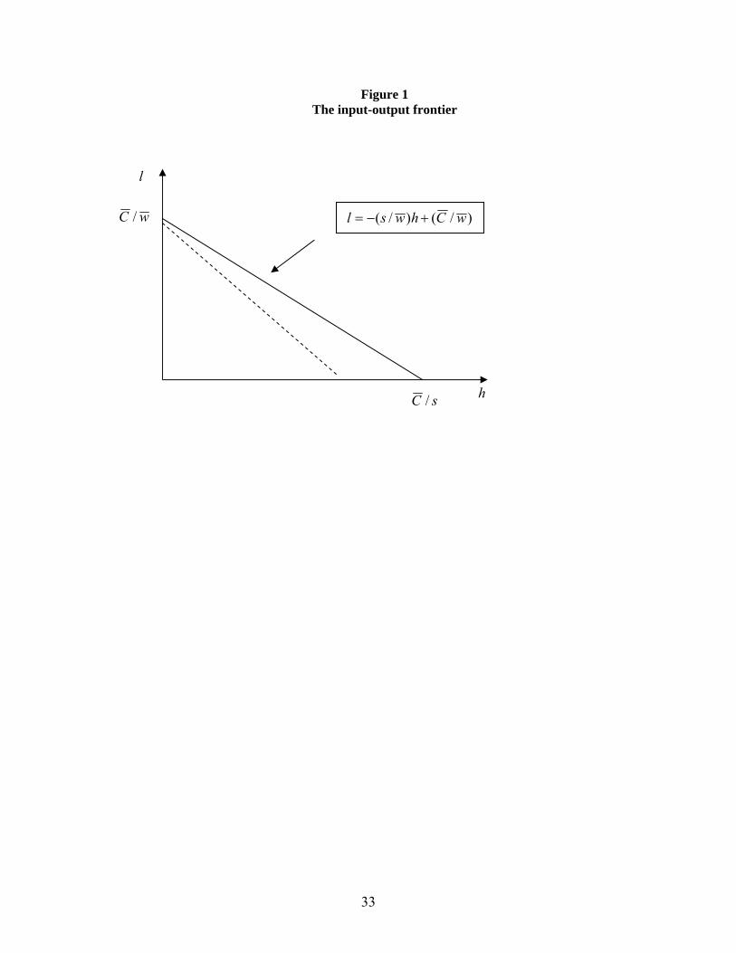
CGhsElEwpE ≥−−−=− )]()()[1()()1( τπτ (7)

The maximum levels of l,h that yield a positive profit higher than the value of the

investment C can be mapped by converting (9) into an equality. An investment will be made if

12

the combined values of l and h are such that they are within the triangle in figure 1, where

)]1(/[ τ−−= GCpC :8

[Insert Figure 1] If the entrepreneur draws input-output coefficients which do not fall within the triangle,

the investment will not be profitable. In addition, since each entrepreneur is small, she doesn’t

take into account the effect of her investment on the skilled-labor wage rate. However, one of the

effects of cost discovery will be that investments by copycats will push up this wage, reducing ex

post the return on capital for the pioneer investor. An increase in the skilled-labor wage will

result in an inward move of the input-output frontier, but only on the h axis, such as is described

by the dotted line in the figure above.

In addition, under certain circumstances, if the country’s producers as a whole face a

downward sloping demand curve, the product price may fall.9 In this case the entire input-output

frontier will move inward toward the origin. If the tax rate increases, the input-output frontier

will also move inward, making investment in discovery less likely.

But, as noted above, there is another kind of discovery: demand discovery. Entrepreneurs

may know the cost structure of a particular good but are uncertain as to whether they can sell it

abroad. Once a market for the product has been created abroad, other producers can take

advantage of the discovery without incurring the costs of opening up the market. In this case, the

investment decision will look like this:

CGshlwpEE ≥−−−=− ])()[1()()1( τπτ (8)

8 For the problem to have a sensible solution, sCwC /,/ must be positive. 9 This is a far from hypothetical case. In Chile, the export discovery of kiwis in the 1970s led in a few years to the collapse of the international price, from which domestic producers did not recover until the late 1980s.

13

In this case, there is a minimum price that makes the venture profitable, and that happens

when the equality in (8) holds. As copycats enter the market for the discovered product, the

skilled-labor wage will be bid up, and the product price may fall, in equilibrium reducing the

profits of the pioneer and copycats alike and discouraging discoveries.

We have thus seen that the profits of the pioneer are eroded by the actions of followers,

either through raising factor rewards or reducing product price. However, the source of the

market failure remains the same: the pioneer takes risks that, if successful, result in easier profits

for others. Therefore, it pays to wait for others to make the discoveries, and the supply of self-

discovery will be suboptimal.

This model has interesting properties. When only sugar production exists, the potential

for opening new sectors is restricted to the resources the government can extract from taxing

sugar profits, which are, at any rate, not reinvested. Therefore, there might be a good argument

for squeezing profits in the traditional sector, since otherwise they will go into the consumption

of the owners of capital. At any rate, the potential for the introduction of new products to the

economy is limited by the narrow tax base. As the tax base widens with the opening up of new

sectors, the government is able to finance new infrastructure projects, thus accelerating growth.

There is, nonetheless, a trade-off between building new infrastructure and opening up new

sectors and investment by the private sector in the existing modern sectors.

Human capital formation is the consequence of new ideas being introduced and existing

skilled workers training unskilled workers. A high rate of investment in human capital (with the

effect of raising μ, in our model) can ease the pressure on the skilled-labor wage that is a

consequence of investment in the modern sector and of the discovery of new products. In

14

addition, the higher the rate of human capital accumulation, the higher will be the rate of new

discoveries.

In this model, government has three roles: investing in sector-specific infrastructure,

which makes discovery possible; subsidizing the cost of discovery, in light of the informational

market failure involved; and raising the rate of skill formation (presumably raising the value of

μ).10 As already noted, it should balance the need for public investment with the drag of taxes on

modern-sector investment, which are financed largely out of retained earning.11

The model can account for several of the constraints to growth discussed in the literature

and illustrates the decision-tree approach to the issue used by Hausmann, Rodrik, and Velasco

(2005). For example, growth can be constrained by a high cost of finance. This would be

reflected in an interest rate spread (φ) that raises the threshold on expected profits required for

self-discovery activities.12 The economy may not be generating enough growth through

discovery because of low appropriability of returns to discovery. Here this takes the form of too

high a tax rate. While taxes finance infrastructure investment, they can also finance consumption.

The rate of new skill formation may be too low to prevent the wages of skilled labor from rising

to levels where they choke off investment. This would be reflected in a low μ in equation (2).

These considerations may explain why successful countries are able to grow faster than

others: they may subsidize discovery activities in various ways; they may keep borrowing costs

low, either by policies that deepen financial markets or by directing credits to winners (see

Amsden, 1989, for the Korean experience); they may use government revenue for investment

rather than consumption; they may keep tax rates reasonable; or they may invest in human

10 The costs of the latter two have not been factored into the model. 11 We are assuming that investment in existing modern sectors are financed from retained earnings, but that funds involved in setting up a new sector are borrowed. 12 If lack of availability of credit to new projects is the problem, then φ is in effect infinite.

15

capital accumulation. Most of the successful countries of Asia have done some or all of these

things. Latin American countries have failed to do a sufficient number of them to ensure an

adequate rate of self-discovery.

III. Trade and Growth in Latin America and Asia, 1980-2003

In this section, we show the plausibility of the hypothesis linking export diversification

and growth by looking at the recent experience of East Asia and LAC. As shown in table 1 and

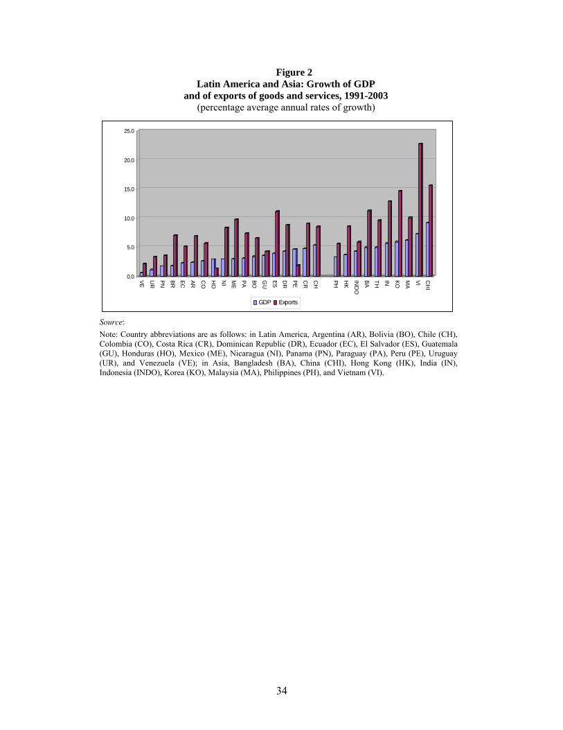
figure 2, the Asian exporters of manufactures grew much faster during 1980-2003 than LAC.

Asian output and exports grew more than twice as fast as Latin America’s. Even if one excludes

the 1980s, the “lost decade” in Latin America, these differences also apply to the period since

1990, although the Asian average rates of growth of output and exports are somewhat lower than

twice the ones recorded by LAC. However, even during the period 1991-2003, the country with

the highest rate of growth of GDP in Latin America (Chile) was surpassed by five of the ten

Asian countries included in the sample.

(Insert Table 1 and Figure 2)

What is interesting about these figures is that the Asian countries consistently grew faster

than LAC, both with regard to GDP and to exports. In fact, the ratio of GDP growth to export

growth is practically identical in the two regions for the two periods shown.

Of course, this does not mean that faster export growth is the key to the success of the

Asian countries relative to their Latin American counterparts, since there are many other

differences between them, but faster export growth, and the factors that underlie it, do appear to

have played a role.

16

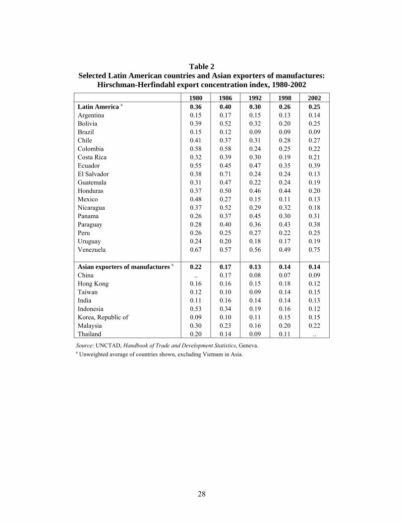
There is evidence that OED has been a trait in the development pattern of Asia. The

proxy for OED that we use here is the HHI13, taken form UNCTAD’s Handbook of Trade and

Development Statistics and measured at the three-digit SITC level. This indicator captures,

however imperfectly, both vertical and horizontal diversification. By vertical diversification is

meant the shift from exporting, say, primary commodities to exporting manufactures. Horizontal

diversification refers to the broadening of the export basket by diversifying into goods within the

same broad category of goods; for example, from grapes with seeds to seedless grapes, or from

coffee for the mass market to gourmet coffee.

As can be seen from table 2, in 1980 Asian countries, on average, had much lower HHI

than LAC; during the period up to 2002 the index declined consistently in all Asian countries,

with the exception) of Taiwan and Korea, where the HHI reach a trough in 1992.14 However, in

2002 these two latter economies exhibited lower HHI than most LAC. Indonesia, a country

whose exports were heavily concentrated on oil in 1980, had a dramatic fall in its HHI over the

1980-2002 period, from 0.53 to 0.12. China, also, while starting with a relatively low HHI in

1986, experienced an important decrease to less than 0.10, a level observed in most developed

countries. Most of the Asian exporters of manufactures are rapidly approaching HHI that are

very similar to those of developed countries.

(Insert Table 2)

Several LAC have been going through a diversification of their exports. Particularly

impressive has been the decline in the HHI of Mexico, Colombia, and, to a lesser extent, Chile. 13 The HHI for country j is defined in the following manner: 2)(∑=

i j

ijj x

xHHI , where xij is the value of exports

of good i by country j and xj represents the value of total exports of country j. 14 These two economies have the highest per capita incomes in the entire sample of middle-income countries, Asian or Latin American. In fact, the International Monetary Fund classifies them as developed economies. Perhaps, the rise in the HHI is evidence of the U-shaped relationship between industrial concentration and income levels found in Imbs and Wacziarg (2003).

17

Argentina exhibits a low HHI for the entire 1980-2002 period. However, their exports remain

more concentrated than those of the Asian exporters of manufactures.

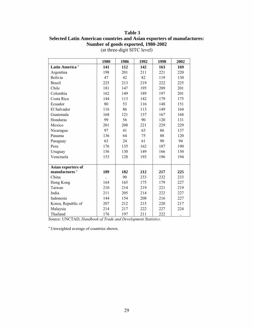
Practically the same picture emerges if one looks at the number of goods exported, also at

the three-digit level (table 3). The maximum number of positions in the SITC classification of

international trade at three digits is 239. Practically all Asian countries are fast approaching that

number. While an increase in the number of goods exported can also be seen in Latin America,

that increase has been more modest, so that the average number of goods exported remains at

about one-half the maximum.

(insert Table 3)

IV. Evidence in Favor of the Portfolio Effect

The portfolio effect of OED on growth claims that export diversification should be

associated with faster growth. If the portfolio effect is indeed at work, the causal relationships

would be those summarized below with the aid of a simple flow chart (figure 3). Export

diversification is related positively to growth through its effects on reducing the variance of

export and GDP growth. As already stated, lessened GDP growth volatility should have a

positive effect on GDP growth.

(Insert Figure 3)

These hypotheses are not falsified by the data available for the period 1980-2003. The

flow chart above would lead one to expect a negative correlation between export diversification

and the variance of export growth, a positive correlation between the variance of export growth

18

and the variance of GDP growth, and a negative correlation between the variance of GDP growth

and the rate of GDP growth.

This is precisely what the data show (see correlation coefficients in figure 2). All

correlation coefficients are of the expected sign and are significantly different from zero at the 1

percent level. Export diversification is measured as DIV = 1 – HHI. Increases in DIV are highly

correlated with declines in the variance of export growth. In turn, a lower variance of export

growth is highly correlated with a lower variance of GDP growth. Finally, a lower variance in

GDP growth is strongly associated with higher GDP growth.

These simple correlations do not amount to a proof of the portfolio effect. But they do

indicate that something like it may indeed be at work.

V. Growth Empirics: Does Export Diversification Add Anything?

In this section, we explore whether export diversification has any explanatory power in a

parsimonious empirical model of growth. Two different variables, proxies for OED, were tested.

One was DIV by itself; a second, diversification-weighted per capita export growth (DIV

interacted with per capita export growth, RX*DIV). As will be noted below, while DIV has the

correct sign and is highly significant, it is the interactive variable that has the most explanatory

power. The intuition behind the inclusion of this interactive variable is that diversification is

more powerful when a country’s exports are growing rapidly than just by itself. Note the

difference between Colombia and Malaysia: both wind up in 2002 with a DIV of 0.78 (HHI of

0.22), but Malaysia’s exports grew at a rate of 10.7 percent in the period 1980-2003, while

Colombia’s grew only at an average rate of 5.7 percent. Diversification-weighted, exports per

19

capita in Malaysia grew at an annual rate of 5.9 percent, while those of Colombia did so at only

2.5 percent. GDP growth in Malaysia averaged 6.4 percent, while it only reached 3.1 percent in

Colombia.

The estimation strategy is to add DIV and RX*DIV to an otherwise standard empirical

model o per capita growth. The variables considered were initial GDP per capita, initial openness

(trade as a percentage of GDP), average fixed capital formation during the period, and the rule of

law index (developed by Kaufmann, Kraay, and Mastruzzi, 2003).15 The model is estimated by

ordinary least squares and by instrumental variables. This latter technique is used in order to

correct possible simultaneity biases stemming from the endogeneity of the growth rate, export

diversification, and the investment rate. The instruments used for the investment rate and for DIV

and RX*DIV were the share of manufactures in exports, population size, and the rule of law

index.

The most suggestive results of the exercise are shown in table 4. In equations (1) and (2),

we control only for initial GDP per capita and openness. DIV and RX*DIV are of the correct sign

and highly significant when they are entered individually into the regression. The inclusion of

both DIV and RX*DIV in an equation (not shown) renders DIV not significantly different from

zero, while the coefficient associated with RX*DIV remains almost unchanged and is still highly

significant. Interestingly, the share of trade in initial GDP plays no role in explaining cross

country variations in growth rates of GDP per capita. Neither is initial income per capita a robust

explanatory variable, as the significance of the coefficient attached to this variable varies quite

sharply between model specifications and estimation techniques. As we shall see, this result is

overturned when we add control variables to the model.

15 A host of different controls were also used, including the average years of schooling in the population aged 15 through 64, but they were not found to add anything to the equation.

20

(Insert Table 4)

Next, we introduce DIV and RX*DIV into a more completely specified model, one that

includes gross fixed investment and the rule of law index. This is done in equations (3) and (4). It

can be seen that this parsimonious model is quite powerful. Initial GDP per capita becomes

highly significant, the openness variable continues to have no role in the explanation of cross

country growth differences, and investment and the rule of law are both of the correct sign and

also highly significant. These results confirm the finding in the literature that growth is positively

related to investment, a hypothesis that goes back to the Harrod-Domar model and is also

compatible with some of the more recent endogenous growth literature.16 The results also lend

credence to the more recent emphasis on institutions as important determinants of growth. The

rule of law is as good as the capacity of governments to enforce it, and such capacity is likely to

depend on a basic social pact. Other things being equal, countries where the government is

perceived as working for the good of society as a whole are better able to enforce the rule of law,

and this may explain the result that higher levels in RL are positively correlated with growth, and

that the coefficient associated to RL is highly significant.

Both variables that attempt to capture OED (DIV and RX*DIV) are highly significant, the

interactive variable more so than DIV. Note that the model explains between 60 percent and two

thirds of the cross country variation in growth rates of per capita GDP. Instrumental variable

estimations raise the value of the coefficients attached to diversification and diversification-

weighted per capita export growth. In equation (3), the coefficient of DIV doubles. In equation

(4), the coefficient of RX*DIV rises just shy of 100 percent. At the same time, the coefficients of 16 Ironically, the profession rediscovered Harrod-Domar in the guise of the AK model. But since economists don’t have much historical memory, nobody has remarked that the AK model is nothing other than the Harrod-Domar model in new clothing. Since much of the growth in productivity in developing countries comes embodied in imported machinery, the importance of investment is likely to be even greater for this group of countries than for developed economies.

21

the other variables remain more or less stable when we go from OLS to IV estimations. This

would seem to support the notion that export diversification, in either of its two formulations, has

been indeed an important contributor to the differences in growth performance in Asia relative to

Latin America.

VI. Growth Differentials: How Much Does OED Explain?

Even if the coefficients attached to our proxies of OED are statistically significant, they

may not add much to the explanation of growth differentials. Through a simple exercise using

the regional average values of DIV, RX*DIV, I/Y, and RL, we can show that our two OED

variables do explain a quantitatively important share of the difference in growth performance

between Asia’s exporters of manufactures and Latin America.

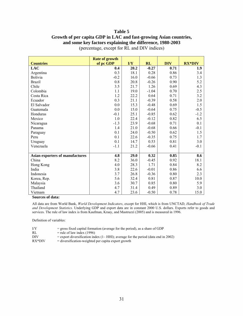
First let us look at what the data for our main variables tell us about these variables that

purportedly explain differences in growth performance. As can be seen in table 5, the rate of

growth of per capita GDP was quite robust in the Asian high performers, while very modest in

LAC. In all explanatory factors, Asia has done better than LAC. Two factors stand out:

investment rates are almost 9 percentage points of GDP higher in Asia, and average

diversification-weighted per capita export growth is 6.7 percentage points higher. This latter

difference arises out of the fact that exports in Asia are both considerably more diversified than

in Latin America and, moreover, have growth faster.

(insert Table 5)

Armed with these data, we undertook a simple calculation of the extent to which each of

the three factors identified above (that is, investment, the rule of law, and export diversification)

22

help to explain growth differentials between Asia’s fast growers and Latin America. The results

are shown in table 6. About 80 percent of the difference in growth rates is explained by

differences in investment rates, the rule of law, and export diversification. Using the coefficients

of equation (3) in table 4 (IV estimation), the main factor explaining growth differences turns out

to be investment, with export diversification adding a not insignificant 0.7 percentage points to

the superior Asian growth performance. When we use the coefficients of equation (4),

diversification-weighted per capita export growth becomes the most important factor explaining

growth differences. This factor, by itself, explains almost 50 percent of the difference in growth

rates between Asian fast-growing exporters of manufactures and LAC. We take this to be

evidence that export growth, in the context of diversification, is the variable pulling GDP growth

and investment.

(insert Table 6)

VII. Conclusions

This paper has developed a theoretical model that attempts to capture the stylized facts of

growth in economies that do not themselves innovate but catch up to the technological frontier

by adding new activities to their production and export structures. The model suggests that

export diversification, insofar as it is symptomatic of broadening comparative advantage, is the

key to economic growth.

The empirical sections of the paper show that export diversification is indeed associated

with higher economic growth. We speculate that there are two channels through which

diversified export growth stimulates output growth. One of them we have called the portfolio

23

effect. Diversification of exports leads to less export volatility, which in turn results in lowered

output volatility. Countries with highly unstable economies grow more slowly than countries that

exhibit more dampened cyclical fluctuations. The data do not contradict this chain of reasoning.

The second effect is associated with the dynamic benefits associated with successful

efforts to diversify comparative advantages. Paramount among are learning and information

externalities. Our results are complementary to the recent findings by Hausmann and Klinger

(2007) that a country’s export pattern is a good predictor of future growth. Countries that export

products associated with the export profile of high-income countries tend to converge rapidly

toward those higher levels of income and, hence, grow more rapidly. We would add that low-

income countries generally have comparative advantages in few (and, not unusually, one) good.

Efforts to diversify away from their traditional comparative advantage are likely to get the

growth process started. It is only through OED that the spillovers of new exports can begin.

These spillovers can be horizontal or horizontal. Any new export produces information that is

useful to other potential entrants into the industry. The emergence of a new sector facilitates the

appearance of other sectors that utilize the same non-tradable inputs or public goods.

The empirical results are congruent with this model. In a cross-country econometric

model of growth, the proxies for OED used (both the degree of export diversification and the

interaction between per capita export growth and export diversification) are highly significant

and make an important contribution to explaining variations in growth rates across countries.

The empirical model shows that variables other than export diversification also play a

role in explaining differences in economic growth between countries. Investment certainly takes

pride of place. It has already been noted that the dynamic Asian economies have rates of

investment that are quite higher than those of the Latin American countries. The strength of

24

investment could well be associated with export growth and export diversification: the more

diversified an economy is, the higher the likelihood that there will be profitable investment

opportunities. In addition, where there is vigorous self-discovery there will also be vigorous

investment. Finally, the more diversified exports are the stronger will be the linkages between

some exporting activities and the rest of the economy.17 In our empirical model, when

diversification-weighted export growth is introduced as an explanatory variable, the quantitative

importance of investment declines sharply. This may very well be an indication that rapid export

growth cum diversification is a powerful incentive to investment.

17 However, investment and export diversification are not so highly correlated that their joint inclusion in the econometric model renders one of them not significant. In fact, the coefficient of the diversification variable is quite robust to the introduction of investment.

25

References

Agosin, M. R. (1999), “Trade and growth in Chile”, CEPAL Review 68, 79-100. Agosin, M. R. and C. Bravo-Ortega (forthcoming, 2007), “The emergence of new successful export activities in Chile”, Latin American Research Network, Inter-American Development Bank, Washington, D.C. Amsden, A. (1989), Asia's Next Giant: South Korea and Late Industrialization, Oxford University Press, New York. Gerschenkron, A. (1962), Economic Backwardness in Historical Perspective, Harvard University Press, Cambridge, MA. Hausmann, R. and D. Rodrik (2003). “Economic Development as Self-Discovery”, Journal of Development Economics 72 (2): 603-633. Hausmann, R., and D. Rodrik (2006). “Doomed to Choose: Industrial Policy as Predicament”. John F. Kennedy School of Government, Harvard University, September. Hausmann, R. D. Rodrik, and A. Velasco (2005), “Growth Diagnostics”, unpublished, John F. Kennedy School of Government, Harvard University. Hausmann, R., and B. Klinger, B. (2007). “The Structure of the Product Space and the Evolution of Comparative Advantage”. CID Working Paper No. 146, Center of International Development, Harvard University, April. Imbs, J., and R. Wacziarg (2003), “Stages of diversification”, American Economic Review 93 (1), 63-86. Jäntti, M., J. Saari, and J. Vartiainen (2005), “Country case study: Finland. Combining growth with equity”. Paper presented at the WIDER Jubilee Conference, June 16-17, 2005, Helsinki. http://www.wider.unu.edu/conference/conference-2005-3/conference-2005-3.htm Kaufmann, D., A. Kraay, and M. Mastruzzi (2005), “Governance matters IV: Governance indicators for 1996-2002”, World Bank Policy Working Paper 3630, Washington, D.C., June. Lewis, W. A. (1954), "Economic Development with Unlimited Supplies of Labour", The Manchester School, May 1954. Romer, P. (1993), “Two Strategies for Economic Development: Using Ideas and Producing Ideas”, Proceedings of the World Bank on Development Economics 1992, Washington, D.C. Vettas, N. (2000), “Investment Dynamics in Markets with Endogenous Demands”, Journal of Industrial Economics, 48(2):189-203.

26

Wade, R. (1990), Governing the Market: Economic Theory and the Role of Government in East Asian Industrialization, Princeton University Press, Princeton, NJ. Wellisz, S., and P. Lam Shin Saw (1993), “Mauritius”, in R. Findlay and S. Wellisz (eds.), The Political Economy of Poverty, Equity, and Growth – Five Small Open Economies, Oxford University Press, Oxford and others.

27

Table 1

GDP and export growth in Latin America and Asia, 1981-2003 (percentage annual change in GDP and real exports of goods and services)

1981-2003 1991-2003 GDP Exports GDP Exports

Growth rates Latin America 2.4 5.3 3.0 6.2 Asia 5.9 11.1 5.5 11.7 GDP-export elasticity Latin America 0.49 0.45 Asia 0.47 0.53

Source: Author’s calculations, based on World Bank. World Development Indicators. Notes: Exports refer to real exports of goods and services (nominal values deflated by the GDP deflator of exports of goods and services). Countries included are, in Latin America, Argentina, Bolivia, Brazil, Chile, Colombia, Costa Rica, Dominican Republic, Ecuador, El Salvador, Guatemala, Honduras, Mexico, Nicaragua, Panama, Paraguay, Peru, Uruguay, Venezuela; in Asia, Bangladesh, China, Hong Kong, India, Indonesia, Korea, Malaysia, Philippines, Thailand, and Vietnam.

28

Table 2 Selected Latin American countries and Asian exporters of manufactures:

Hirschman-Herfindahl export concentration index, 1980-2002

1980 1986 1992 1998 2002 Latin America a 0.36 0.40 0.30 0.26 0.25 Argentina 0.15 0.17 0.15 0.13 0.14 Bolivia 0.39 0.52 0.32 0.20 0.25 Brazil 0.15 0.12 0.09 0.09 0.09 Chile 0.41 0.37 0.31 0.28 0.27 Colombia 0.58 0.58 0.24 0.25 0.22 Costa Rica 0.32 0.39 0.30 0.19 0.21 Ecuador 0.55 0.45 0.47 0.35 0.39 El Salvador 0.38 0.71 0.24 0.24 0.13 Guatemala 0.31 0.47 0.22 0.24 0.19 Honduras 0.37 0.50 0.46 0.44 0.20 Mexico 0.48 0.27 0.15 0.11 0.13 Nicaragua 0.37 0.52 0.29 0.32 0.18 Panama 0.26 0.37 0.45 0.30 0.31 Paraguay 0.28 0.40 0.36 0.43 0.38 Peru 0.26 0.25 0.27 0.22 0.25 Uruguay 0.24 0.20 0.18 0.17 0.19 Venezuela 0.67 0.57 0.56 0.49 0.75 Asian exporters of manufactures a 0.22 0.17 0.13 0.14 0.14 China .. 0.17 0.08 0.07 0.09 Hong Kong 0.16 0.16 0.15 0.18 0.12 Taiwan 0.12 0.10 0.09 0.14 0.15 India 0.11 0.16 0.14 0.14 0.13 Indonesia 0.53 0.34 0.19 0.16 0.12 Korea, Republic of 0.09 0.10 0.11 0.15 0.15 Malaysia 0.30 0.23 0.16 0.20 0.22 Thailand 0.20 0.14 0.09 0.11 ..

Source: UNCTAD, Handbook of Trade and Development Statistics, Geneva. a Unweighted average of countries shown, excluding Vietnam in Asia.

29

Table 3 Selected Latin American countries and Asian exporters of manufactures:

Number of goods exported, 1980-2002 (at three-digit SITC level)

1980 1986 1992 1998 2002 Latin America a 141 112 142 163 169 Argentina 198 201 211 221 220 Bolivia 47 42 82 119 130 Brazil 225 213 219 222 225 Chile 181 147 195 209 201 Colombia 162 149 189 197 201 Costa Rica 144 113 142 179 175 Ecuador 80 53 116 148 151 El Salvador 116 86 113 149 164 Guatemala 168 121 137 167 168 Honduras 99 56 90 120 131 Mexico 201 208 221 229 229 Nicaragua 97 41 63 86 137 Panama 136 64 75 88 120 Paraguay 63 24 61 90 94 Peru 176 135 162 187 190 Uruguay 156 130 149 166 150 Venezuela 153 128 193 196 194 Asian exporters of manufactures a 189 182 212 217 225 China .. 90 233 232 233 Hong Kong 164 165 175 179 227 Taiwan 210 214 219 221 219 India 211 205 214 222 227 Indonesia 144 154 208 216 227 Korea, Republic of 207 212 215 220 217 Malaysia 214 217 222 227 224 Thailand 176 197 211 222 ..

Source: UNCTAD, Handbook of Trade and Development Statistics. a Unweighted average of countries shown.

30

Table 4 An empirical model of growth

Dependent variable: Average annual rate of growth of GDP per capita, 1980-2003

(1) (2) (3) (4) Explanatory variables OLS IV OLS IV OLS IV OLS IV log YPC80 -0.102

(-0.87) -0.366

(-2.57)* -0.014 (-0.16)

-0.080 (-0.72)

-0.800 (-6.99)**

-0.717 (-5.41)**

-0.683 (-5.94)**

-0.581 (-3.92)**

TRADE80 0.006 (1.51)

0.014

0.005 (1.62)

0.006 (1.68)+

-0.001 (-0.44)

0.000 (0.01)

-0.000 (-0.01)

0.003 (0.83)

I/Y 0.192 (9.12)**

0.249 (4.88)**

0.159 (6.49)**

0.119 (3.09)**

RL 1.345 (7.30)**

0.949 (3.48)**

1.198 (6.41)**

0.911 (3.53)**

DIV 4.646 (5.12)**

12.147 (4.71)**

2.309 (3.59)**

5.05 (2.92)**

RX*DIV 0.326 (9.37)**

0.465 (9.26)**

0.176 (5.43)**

0.312 (5.65)**

Adj. R2 0.165 - 0.427 0.365 0.655 0.608 0.677 0.640 No. of obs. 124 118 118 117 113 112 109 108 Sources of data: All data are from World Bank, World Development Indicators, except for HHI, which is from UNCTAD, Handbook of Trade and Development Statistics. Underlying GDP and export data are in constant 2000 U.S. dollars. Exports refer to goods and services. The rule of law index is from Kaufman, Kraay, and Mastruzzi (2005) and is measured in 1996. Constant not shown; t ratios in parenthesis; IV estimations with robust standard errors. * Significantly different from zero at the 10 percent level. ** Significantly different from zero at the 5 percent level. *** Significantly different from zero at the 1 percent level. Definition of variables: YPC80 = GDP per capita in 1980 TRADE80 = exports plus imports divided by GDP in 1980 I/Y = gross fixed capital formation (average for the period), as a share of GDP RL = rule of law index (1996) DIV = export diversification index (1– HHI); average for the period (data end in 2002) RX*DIV = diversification-weighted rate of growth of per capita exports Instrumental variables used for DIV, RX*DIV and I/Y: share of manufactures in GDP, population size, and rule of law.

31

Table 5 Growth of per capita GDP in LAC and fast-growing Asian countries,

and some key factors explaining the difference, 1980-2003 (percentage, except for RL and DIV indices)

Countries Rate of growth

of pc GDP I/Y RL

DIV

RX*DIV LAC 0.4 20.2 -0.27 0.71 1.9 Argentina 0.3 18.1 0.28 0.86 3.4 Bolivia -0.2 16.0 -0.66 0.73 1.3 Brazil 0.8 20.8 -0.26 0.90 5.2 Chile 3.5 21.7 1.26 0.69 4.3 Colombia 1.1 19.0 -1.04 0.70 2.5 Costa Rica 1.2 22.2 0.64 0.71 3.2 Ecuador 0.3 21.1 -0.39 0.58 2.0 El Salvador 0.0 15.3 -0.48 0.69 1.5 Guatemala 0.0 15.0 -0.64 0.75 -0.5 Honduras -0.1 25.1 -0.85 0.62 -1.2 Mexico 1.0 22.4 -0.12 0.82 6.5 Nicaragua -1.3 23.9 -0.68 0.71 0.1 Panama 1.4 21.0 -0.68 0.66 -0.1 Paraguay 0.1 24.0 -0.50 0.62 1.5 Peru 0.1 22.6 -0.35 0.75 1.7 Uruguay 0.1 14.7 0.53 0.81 3.0 Venezuela -1.1 21.2 -0.66 0.41 -0.1 Asian exporters of manufactures 4.8 29.0 0.32 0.85 8.6 China 8.2 36.0 -0.45 0.92 18.1 Hong Kong 4.0 28.3 1.71 0.84 8.2 India 3.8 22.6 -0.01 0.86 6.6 Indonesia 3.7 26.8 -0.36 0.80 2.3 Korea, Rep. 5.6 32.4 0.81 0.87 10.0 Malaysia 3.6 30.7 0.85 0.80 5.9 Thailand 4.7 31.4 0.49 0.89 3.0 Vietnam 4.7 23.6 -0.50 0.78 15.0 Sources of data: All data are from World Bank, World Development Indicators, except for HHI, which is from UNCTAD, Handbook of Trade and Development Statistics. Underlying GDP and export data are in constant 2000 U.S. dollars. Exports refer to goods and services. The rule of law index is from Kaufman, Kraay, and Mastruzzi (2005) and is measured in 1996.

Definition of variables:

I/Y = gross fixed capital formation (average for the period), as a share of GDP RL = rule of law index (1996) DIV = export diversification index (1– HHI); average for the period (data end in 2002) RX*DIV = diversification-weighted per capita export growth

32

Table 6 Explaining the difference in growth rates between LAC

and the Asian exporters of manufactures (percentage)

Calculation I Calculation II Growth differential 4.4 4.4 Contribution of: Investment 2.2 1.0 Rule of law 0.6 0.5 Export diversification 0.7 Diversification-weighted pc export growth 2.1 Total of above factors 3.5 3.6

Source: Results in table 4 and data in table 5. Note: In calculation I, the coefficients of equation (3, IV) were used; calculation II is based on the coefficients of equation (4, IV).

33

Figure 1 The input-output frontier

l

h

)/()/( wChwsl +−=

sC /

wC /

34

Figure 2 Latin America and Asia: Growth of GDP

and of exports of goods and services, 1991-2003 (percentage average annual rates of growth)

0.0

5.0

10.0

15.0

20.0

25.0

VE UR

PN BR EC

AR CO

HO

NI

ME

PA BO GU

ES DR

PE CR

CH

PH HK

IND

O

BA TH IN KO MA

VI CH

I

GDP Exports

Source: Note: Country abbreviations are as follows: in Latin America, Argentina (AR), Bolivia (BO), Chile (CH), Colombia (CO), Costa Rica (CR), Dominican Republic (DR), Ecuador (EC), El Salvador (ES), Guatemala (GU), Honduras (HO), Mexico (ME), Nicaragua (NI), Panama (PN), Paraguay (PA), Peru (PE), Uruguay (UR), and Venezuela (VE); in Asia, Bangladesh (BA), China (CHI), Hong Kong (HK), India (IN), Indonesia (INDO), Korea (KO), Malaysia (MA), Philippines (PH), and Vietnam (VI).

35

Figure 3

The portfolio effect of export diversification on growth in 1980-2003: a simple flow chart

The values of ρ represent the correlation coefficients between the variables in the two adjacent boxes measured without the Δ’s. All of them are significant at the 1 percent level. The data used are for 106 countries over the 1980-2003 period. The data are from World Bank, World Development Indicators; and UNCTAD, Handbook of Trade and Development Statistics. Export growth refers to goods and services in 2000 US dollars. GDP growth data are in 2000 US dollars.

Export diversification

Export growth variance

GDP growth variance

GDP growth

ρ = -0.420**

ρ = 0.377**

ρ = -0.406**