empirical modeling of systematic spectrophotometric errors

Ro S. Berns Kevin Y H. Petersen* Munsell Color Science Laboratory Center for Imaging Science Rochester Institute of Technology Post Office Box 9887 Rochester, New York 14623-0887

Empirical Modeling of Systematic Spectrophotometric Errors

Spectrophotometers, as electro-mechanical-optical devices, perform at a Jinite level of accuracy. This accuracy is limited by such factors as monochromator design, detector linearity, and cost. Generally, both the diagnosis and correction of spectrophotometric errors require a number of calibrated standard reference materials and considerable effort and commitment on the part of the user. A technique using multiple linear regression has been developed, based on the measurement of several suitably chosen standard reference materials, to both diagnose and correct systematic spectrophotometric errors, including photometric zero errors photometric linear and reonlinear scale errors, wavelength linear and nonlinear scale errors, and bandwidth errors. The use of a single chromatic ceramic tile to correct systematic errors improved the colorimetric accuracy of a set of chromatic and neutral tiles by a factor of two for a typical industrial-oriented spectrophotometer . Greater improvement can be achieved by increasing the number of tiles and perj+orming a separate regression at each measured wavelength., These techniques have been extremely useful in improving inter-instrument agreement for instruments with similar geometry.

Introduction

In general, spectrophotometers perform at a finite level of accuracy. As electro-mechanical-optical devices, they exhibit measurement errors relative to a theoretical error-free instrument that users must accept. These errors can be con- veniently divided into systematic and random errors. Sys- tematic errors include errors resulting from wavelength, bandwidth, detector linearity, nonstandard geometry, and

*Present address: The Pentagon, Washington, DC 0 1988 by John Wiley & Sons, Inc.

Volume 13, Number 4, August 1988

polarization. Random errors result from drift, electronic noise, and sample presentation. Qualitatively, systematic errop affect accuracy while random errors affect repeata- bility. The distinction between the two classifications de- pends on the situation. Thermochromism, i.e., a change in color (spectral reflectance factor) caused by a change in temperature,' would be classified as a random error if the temperature of a thermochromic material unexpectedly changed before a measurement. If a thermochromic material was calibrated at one temperature and measured at another, the error in spectral reflectance factor would be systematic. The most prevalent errors in modern instruments are associated with stray light, wavelength scale, bandwidth, reference white calibration, and thermochromism.

Carter and Billmeye? summarized an Inter-Society Color Council technical report that described material standards for calibrating, performance testing, and diagnostic check- ing of color-measuring instruments. This article provided an excellent overview on the proper methodologies to cal- ibrate spectrophotometers and diagnose systematic errors. Unfortunately, many industrial laboratories do not, as a matter of course, test instrument performance. In addition, many current instruments provide spectral data only at such discrete wavelength intervals as 10 or 20 nm. The difficulties in accurately diagnosing wavelength errors, in particular, for these instruments has further hampered diagnostic ef- forts.

Diagnosis, however, is only the first step to improving instrument performance. The second step is to correct an instrument's systematic errors. This involves both mechanical and mathematical adjustments. In many industrial environments only mechanical adjustments tend to be made. Techniques to correct small systematic errors mathematically, performed routinely by standardizing laboratories, are calculation intensive and beyond the scope of most industrial laboratories. Billmeyer and Alessi3 as- sessed the colorimetric accuracy of typical color-measur-

CCC 0361 -231 7/88/040243-14$04.00 243

ing instruments in which only mechanical adjustments were Photometric Zero Error made. These instruments had an average colorimetric error of about one CIELAB color-difference unit compared with results from a standardizing laboratory when rnea- suring the reflectance factor of chromatic and achromatic tiles. Based on informal investigations in our laboratory, current color-measuring instruments designed for the industrial community are capable of better performance when properly maintained. Nonetheless, the lack of agreement between instruments of similar geometry but different manufacturers and the difficulties in maintaining close agreement for groups of “identical” instruments suggest that more sophisticated techniques to reduce systematic errors may be needed.

During the past several years, we have analyzed various mathematical techniques to diagnose and correct systematic errors inherent in our industrial-oriented spectrophotometers in order to improve their colorimetric performance and inter- instrument agree~nent .~ This article describes one method particularly suited to industrial environments.

The method is based on the use of multiple linear regression in which systematic errors, modeled by a series of linear equations, are minimized in a least-squares sense between instrumental measurements and “standardized’ measurements. This method was outlined by Robertson.s He dem- onstrated its utility in diagnosing photometric zero errors, linear photometric scale errors, and linear wavelength errors in a General Electric recording spectrophotometer. We have done further testing of his equations, derived equations to describe nonlinear systematic errors, and extended the statistical method by including stepwise linear regression. This technique has been applied to reflectance-factor measurements but is also suitable to transmittance measurements. Since most industrial-oriented spectrophotometers report percent reflectance factor rather than reflectance factor, the remainder of this article and all calculations are based on units of percent reflectance factor.

Mathematical Description of Systematic Errors

The method is based on the use of multiple linear regression, which requires modeling systematic errors as a series of linear equations. It should be noted that a linear model implies only that the parameters are linear; the model may bc nonlinear. For example, it is well known that the relationship between luminous reflectance factor and Munsell value can be well modeled by a fifth-order polynomial, a nonlinear function. Multiple linear regression can be used to calculate the “weightings” of each order of the model, i.e., to calculate the parameters of the model. The success of the technique is limited by the accuracy of the postulated model. If the relationship between luminous reflectance factor and Munsell value was assumed to follow a straight line (a first-order polynomial), the model fit would be poor. With respect to modeling systematic spectrophotometric errors, greater knowledge of the mechanics of the device will enable a more accurate estimate of the appropriate model.

A photometric zero error is an offset of the entire photometric scale. It is often caused by stray light associated with input optics, the use of a black trap with a finite reflectance factor, or ignoring detector dark current. It is expressed as

RLA) Rrn(h) + BU (1)

where Rr(X) is the true or reference reflectance factor, R,(h) is the measured reflectance factor to be evaluated, and Bo is the photometric zero error.

Photometric Linear Scale Error

A photometric linear scale error is an error that is proportional to the reflectance-factor measurement. It is most often caused by an improperly calibrated white standard (“100%-line error”) or one that has physically changed since initial calibration. It is expressed as

RLh) = R m ( h ) + BlRm(X) ( 2 )

where B1 is the photometric scale error.

Photometric Nonlinear Scale Error

A photometric nonlinear scale error is most often caused by detector nonlinearity. Since spectrophotometers are calibrated such that zero and 100% reflectance factor are set, a nonlinear error can be approximately expressed as

Rr(X) = R m ( h ) + Bzl100 - Rm(A)IRrn(X) (3)

where B2 represents a nonlinear photometric scale error. It is helpful to think of 100 - R,,(h) as a nonlinear weighting function of the photometric scale error. This quadratic function typifies errors that are small at the ends of the photometric scale and larger in the middle.

Wavelength Linear Scale Errors

A wavelength scale error is an error in the measured reflectance factor resulting from a shift in the wavelength scale. The resulting error in reflectance factor is approximately proportional to the first derivative of the measured reflectance factor. It is expressed as

R,(X) = R,(X) + B,dR,/dh (4)

where B3 is the wavelength scale error and dR,ldh is the first derivative of R,(X) with respect to wavelength. The first derivative is equal to

where i is an index of wavelength. In this study the first derivatives of the first and last measured wavelengths were set equal to those of the second and second-to-last measured wavelengths, respectively.

244 COLOR research and application

Wavelength Nonlinear Scale Error

Many instruments, in fact, have wavelength scale errors that are nonlinear with respect to wavelength. Based on evaluating several industrial instruments using didymium filters and calculating inflection points, wavelength scales, in a sense, were weighted by functions approximately expressed as

(6) R,(h) = R,(h) + B,w,(h)dR,/dX

R,(h) = R,(A) + B5w2(X)dRm/dA

w2(X) = sin 2 r (X/200)

(8)

t 9) where B4 and B5 are nonlinear wavelength scale errors. Weighting function wl(X) is identical to the quadratic function described in eq. (4), except scaled to wavelength. Weighting function w2(h) is a one-and-one-half-cycle sine wave. This would represent an instrument with both positive and negative wavelength errors.

Equations (4), (6), and (8) represent three different models of an instrument’s wavelength error. Depending on the dispersing element in the monochromator and the scanning mechanism, different functions may be more nearly appropriate. The dispersing elements in many spectrophotometers are nonlinear by definition. Manufacturers, as a matter of course, characterize the nonlinearity and appropriately ac- count for the nonlinearity mechanically or mathematically. In theory, wavelength errors should reduce to linear errors that are relatively simple to correct mechanically. In practice, the limiting systematic error in most industrial-oriented instruments remains wavelength error, often of a nonlinear nature.

Bandwidth Error

If the spectral bandwidth of a spectrophotometer varies with wavelength or if the bandwidth is excessively large, an error in the measured reflectance factor can occur. As- suming a symmetrical bandwidth function, the resulting error is proportional as a first approximation to the second derivative of the measured reflectance factor with respect to wavelength. It is expressed as

(10)

where B6 is the bandwidth error and d2R,ldh2 is the second derivative of R,(X) with respect to wavelength. It is equal to

R,(X) = R,(h) + B6d2R,/dX2

(d2RldX2); (11) - R(Xi+1, + R(Xi-1) - %(A) -

(hi+l - L l > 2

Regression Model

Seven systematic errors considered in this article have been described by linear equations. They are summarized in Table

TABLE I . Summary of the systematic errors and their modeled equations considered in this article, including their notation and the notation of the parameters.

Svstematic error Parameter Model

Photometric zero Photometric linear

scale Photometric nonlinear

scale Wavelength linear

scale Wavelength nonlinear

scale (quadratic) Wavelength nonlinear

scale (sine wave) Bandwidth

I. For notational ease, the measured reflectance factors and their associated functional forms representing the seven systematic errors can be abbreviated by variables Xo(h) through X6(h). For example, XI@) = R,(X) and X2(h) = R,(h) [lo0 - &,(A)]. Xo(X) is a special case referred to as a “dummy” variable and is equal to unity.

Suppose that a spectrophotometer had all these systematic errors. The difference between the measured reflectance factor and the actual reflectance factor of a material could be expressed as

M A ) - R A M = Bdr,(X) +BIXI(X) + . . . + B&&) + e(h) (12)

where Bo, B1, . . . , B6 are the weighting parameters of each systematic error and e(X) is the sum-of-squares residual error not accounted for by this model. Suppose, also, that the spectrophotometer measures from 400 through 700 nm in 10-nm increments. Thus, eq. (12) actually represents 31 equations. These equations can be written in terms of ma- trices:

Y = X B + e (13)

where Y is a (31 x 1) column vector containing R,(X) - R,(X) as its elements, X is a (31 X 7) matrix containing the measured functions of reflectance factor, B is a (7 x 1) column vector containing the error parameters, and e is a (3 1 X 1) column vector containing the sum-of-squares residual errors. Multiple linear regression estimates the magnitude of the elements in the error matrix B such that the elements in the residual error matrix e are minimized.6 The elements in matrix B are referred to as the regression coefficients. The magnitudes of the regression coefficients Bo- B6 indicate the magnitudes of the corresponding systematic errors for the modeled instrument. The magnitudes of the elements in matrix e indicate the model fit. A variety of statistical significance tests can be performed to evaluate the model fit.6 The most important statistic to evaluate would be the regression analysis of variance.

Once the regression coefficients are estimated, the measured reflectance factor can be corrected by

&(A) = R,(h) + B&o(A) + . . . + B&j(h) (14)

where Rc(h) is the corrected reflectance factor.

Volume 13, Number 4, August 1988 245

The above regression model has been developed to correct systematic errors. Each error described by a linear equation is a function of the measured reflectance factor. This is the inverse of diagnostic spectrophotometry in which the measured data are described as a function of the true data. For example, we describe an instrument as having a wavelength error. Implied in this statement is that the measured data are a corruption of the theoretical error-free true data. In Robertson’s research,’ the errors described by linear equations were functions of the true data. The advantage of Robertson’s method is that the elements in the coefficient matrix B directly describe systematic errors. When the systematic errors are functions of the measured data, eq. (14) must be inverted to yield regression coefficients that are functions of the true data, enabling diagnosis of systematic errors. One advantage in regressing on measured data is the gain in precision in correcting wavelength errors, particularly for highly chromatic samples. Because the first and second derivatives are sample-dependent and asymmetric, it seems intuitive to regress on the measured data. This is increasingly important as the wavelength error increases.

In a strict statistical sense, regression methods typically used to estimate the regression coefficients assume the response variable is subject to error but the predictor variables are not.6 Both Robertson’s equations and our equations do not obey this assumption. The predictor variables in Robertson’s equations are functions of standardizing- laboratory data; in the current work, the predictor variables are functions of measured data. The former case contains small systematic and random errors while the latter case contains random errors and systematic errors to be modeled by the regression. Given that the spectrophotometric systematic errors to be modeled are much greater than random errors and standardizing-laboratory systematic errors, we have assumed that the random errors and standardizing-laboratory systematic errors are negligible. As a consequence, the required assumption that predictor variables are not subject to error is upheld and the usual methods for estimating the regression coefficients can be employed. Therefore, the error matrix e represents error resulting from modeling lack of fit. The assumption that the random error is negligible has the further advantage of eliminating the need to test whether spectrophotometric random errors are normally distributed, another required assumption in order to apply multiple linear regression techniques. Previous research by Billmeyer and Alessi3 indicates that spectrophotometric measurements are not normally distributed.

To diagnose systematic errors using the regression coefficients optimized to correct systematic errors, we assumed that the calculations of the first and second derivatives are invariant to photometric errors. Calculations4 on inflection- point determination with simulated photometric errors support this assumption. The following equations can be used to estimate the most important systematic errors relative to true data enabling error diagnosis:

where subscript c refers to correction parameters generated in the regression and subscript d refers to the diagnostic error parameters. Equations ( 1 5 ) to ( 1 8) represent the in- version of eq. (14) containing error terms X o ( A ) , X,(A), X3( A ) , and &(A).

Optimization to a Single Standard Reference Material

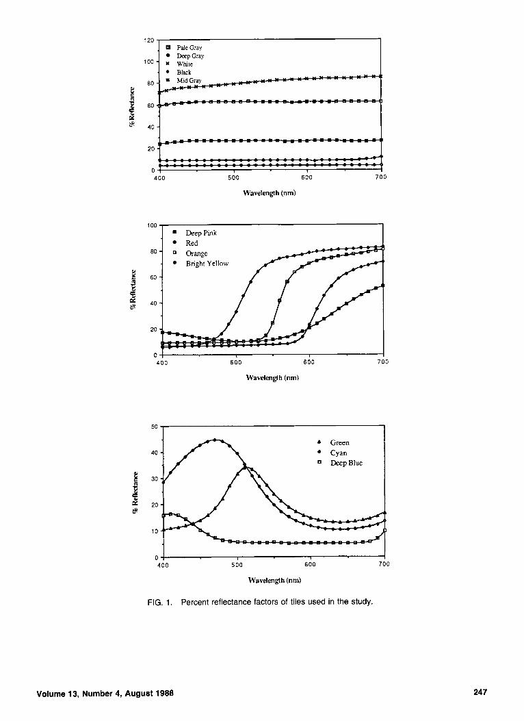
Preliminary calculations4 indicated that this method was quite effective in correcting systematic errors. To have a technique with significant industrial utility, we were interested in identifying one or two SRMs that could be used to accurately diagnose and correct typical systematic errors. The British Ceramic Research Association (BCRA) Series I1 ceramic tiles’ were selected for study, with the omission of the difference gray and green tiles. We also used an Ever- Black glass tile manufactured by Yoneda Glass Bead Company8 and the NBS SRM-2019 white ceramic tile to have samples near the two extremes of the photometric scale. The percent spectral reflectance factors for these 12 tiles are shown in Fig. 1 . Total reflectance factors (specular component included) were used throughout this study.

The actual* reflectance factors of each tile were “cor- rupted” by introducing the following simulated error:

R,i,(A) = R,(A + 5 ) + O.OSR,(A + 5 ) + 5.00 (19)

where R,,(A) is the simulated reflectance factor and R,(A + 5 ) is the actual reflectance factor at an additional 5 nm. If A = 500 nm, the actual reflectance factor at 505 nm was used. R,y,,(A) corresponded to a 5% photometric linear scale error, a +5.00% reflectance factor zero error, and a 5-nm wavelength scale error. For example, if R,(400 nm) = 20.00% and R,(405 nm) = 22.00%, then RSi,(400 nm) = 22.00 + O.OS(22.00) + 5.00 = 28.10%. In practice, an instrument with systematic errors of this magnitude would be in serious need of mechanical adjustments. We have used this order of magnitude to amplify differences in each tile’s effectiveness as a potential diagnostic standard.

The regression technique was applied to each tile using three of the six systematic errors described above: X,, the photometric zero error; X I , the photometric linear scale error; and X 3 , the wavelength linear scale error. If a tile was

*The reference instrument was a Zeiss DMC-26 spectrophotometer. On the basis of the results of a measurement assurance program with the National Bureau of Standards, we found this instrument had an average systematic error in transmittance of 0.00099 (representative of both photometric linearity and photometric zero error) and an average systematic error in wavelength of 0.25 nm. The constant bandwidth was 9.1 nm. The random error of this instrument is unknown. For the purposes of this study, the instrument was assumed to be error-free.


PaleGray DeepGray

. * Black

60 <<

J

20 -

400 500 600

Wavelength (nm)

700

100 . DeepPink Red Orange Bright Yellow

o f I I I 400 500 600 7 0 0

Wavelength (nm)

0 4 I I

400 500 600 I

Wavelength (nm)

FIG. 1. Percent reflectance factors of tiles used in the study.


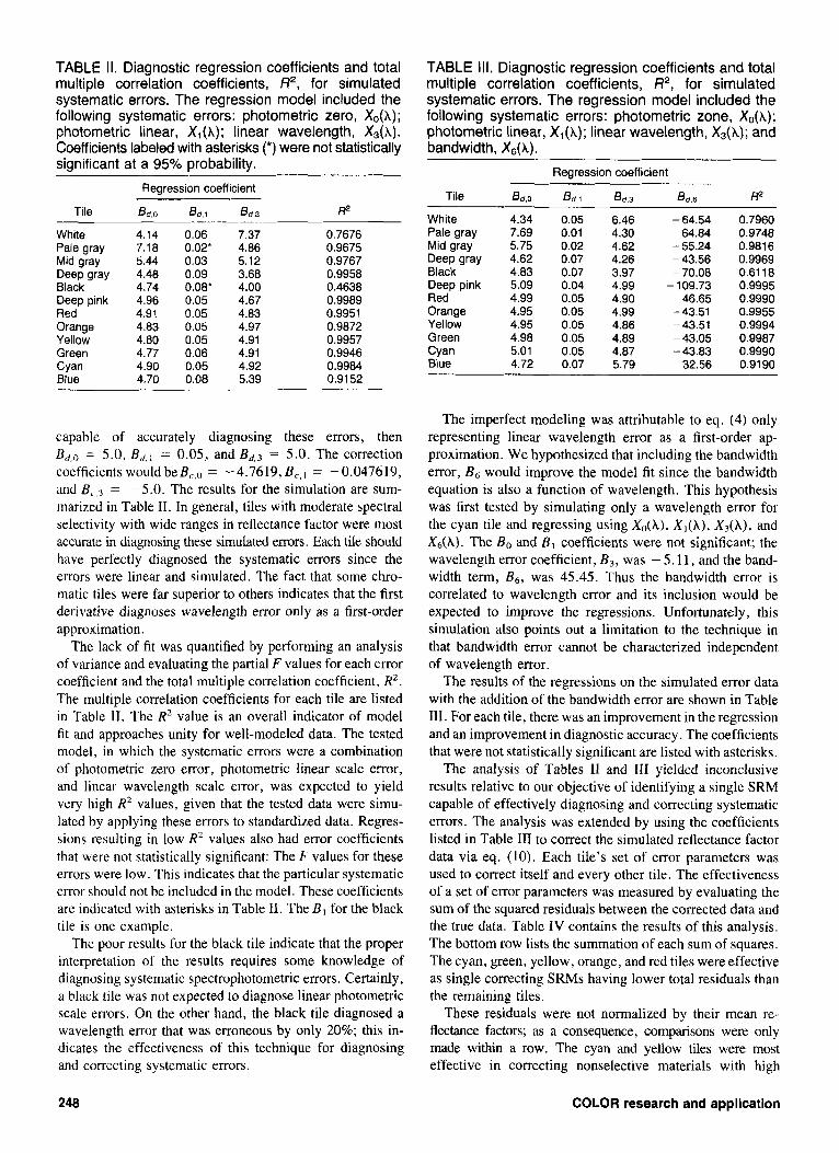
TABLE II. Diagnostic regression coefficients and total multiple correlation coefficients, R2, for simulated systematic errors. The regression model included the following systematic errors: photometric zero, X,(h); photometric linear, X,(X); linear wavelength, X3(h). Coefficients labeled with asterisks (*) were not statistically significant at a 95% probability.

Regression coefficient

Tile 6 d , o 6 d . l 8 6 . 3 R*

White Pale gray Mid gray Deep gray Black Deep pink Red Orange Yellow Green Cyan

4.14 0.06 7.18 0.02' 5.44 0.03 4.48 0.09 4.74 0.08' 4.96 0.05 4.91 0.05 4.83 0.05 4.80 0.05 4.77 0.06 4.90 0.05

7.37 4.86 5.12 3.68 4.00 4.67 4.83 4.97 4.91 4.91 4.92

0.7676 0.9675 0.9767 0.9958 0.4638 0.9989 0.9951 0.9872 0.9957 0.9946 0.9984

TABLE Ill. Diagnostic regression coefficients and total multiple correlation coefficients, R2, for simulated systematic errors. The regression model included the following systematic errors: photometric zone, &(A); photometric linear, X,(h); linear wavelength, X&); and bandwidth, X&).

Regression coefi icient

Tile Bd,o 6 d . i 84.3 Bd.6 R2

White Pale gray Mid gray Deep gray Black Deep pink Red Orange Yellow Green Cyan Blue

4.34 7.69 5.75 4.62 4.83 5.09 4.99 4.95 4.95 4.98 5.01 4.72

0.05 6.46 0.01 4.30 0.02 4.62 0.07 4.26 0.07 3.97 0.04 4.99 0.05 4.90 0.05 4.99 0.05 4.86 0.05 4.89 0.05 4.87 0.07 5.79

- 64.54 - 64.84 - 55.24 - 43.56 - 70.08 - 109.73 -46.65 - 43.51 - 43.51 - 43.05 - 43.83 -32.56

0.7960 0.9748 0.9816 0.9969 0.61 18 0.9995 0.9990 0.9955 0.9994 0.9987 0.9990 0.91 90

Biue 4.70 0.08 5.39 0.91 52

capable of accurately diagnosing these errors, then Bd,O = 5.0, Bfl, = 0.05, and Bd,3 = 5.0. The correction coefficients would beB,,o = -4.7619,BC,, = -0.047619, and B c , , = - 5.0. The results for the simulation are summarized in Table 11. In general, tiles with moderate spectral selectivity with wide ranges in reflectance factor were most accurate in diagnosing these simulated errors. Each tile should have perfectly diagnosed the systematic errors since the errors were linear and simulated. The fact that some chromatic tiles were far superior to others indicates that the first derivative diagnoses wavelength error only as a first-order approximation.

The lack of fit was quantified by performing an analysis of variance and evaluating the partial F values for each error coefficient and the total multiple correlation coefficient, R 2 . The multiple correlation coefficients for each tile are listed in Table 11. The R2 value is an overall indicator of model fit and approaches unity for well-modeled data. The tested model, in which the systematic errors were a combination of photometric zero error, photometric linear scale error, and linear wavelength scale error, was expected to yield very high R2 values, given that the tested data were simulated by applying these errors to standardized data. Regres- sions resulting in low R2 values also had error coefficients that were not statistically significant: The F values for these error5 were low. This indicates that the particular systematic error should not be included in the model. These coefficients are indicated with asterisks in Table 11. The B1 for the black tile is one example.

The poor results for the black tile indicate that the proper interpretation of the results requires some knowledge of diagnosing systematic spectrophotometric errors. Certainly, a black tile was not expected to diagnose linear photometric scale errors. On the other hand, the black tile diagnosed a wavelength error that was erroneous by only 20%; this indicates the effectiveness of this technique for diagnosing and correcting systematic errors.

The imperfect modeling was attributable to eq. (4) only representing linear wavelength error as a first-order approximation. We hypothesized that including the bandwidth error, B6 would improve the model fit since the bandwidth equation is also a function of wavelength. This hypothesis was first tested by simulating only a wavelength error for the cyan tile and regressing using X&), X,(h) , X,(h), and X 6 ( X ) . The Bo and B1 coefficients were not significant; the wavelength error coefficient, B,, was - 5.11, and the bandwidth term, B6, was 45.45. Thus the bandwidth error is correlated to wavelength error and its inclusion would be expected to improve the regressions. Unfortunately, this simulation also points out a limitation to the technique in that bandwidth error cannot be characterized independent of wavelength error.

The results of the regressions on the simulated error data with the addition of the bandwidth error are shown in Table Ill. For each tile, there was an improvement in the regression and an improvement in diagnostic accuracy. The coefficients that were not statistically significant are listed with asterisks.

The analysis of Tables 11 and 111 yielded inconclusive results relative to our objective of identifying a single SRM capable of effectively diagnosing and correcting systematic errors. The analysis was extended by using the coefficients listed in Table I11 to correct the simulated reflectance factor data via eq. (10). Each tile's set of error parameters was used to correct itself and every other tile. The effectiveness of a set of error parameters was measured by evaluating the sum of the squared residuals between the corrected data and the true data. Table 1V contains the results of this analysis. The bottom row lists the summation of each sum of squares. The cyan, green, yellow, orange, and red tiles were effective as single correcting SRMs having lower total residuals than the remaining tiles.

These residuals were not normalized by their mean reflectance factors; as a consequence, comparisons were only made within a row. The cyan and yellow tiles were most effective in correcting nonselective materials with high

COLOR research and application

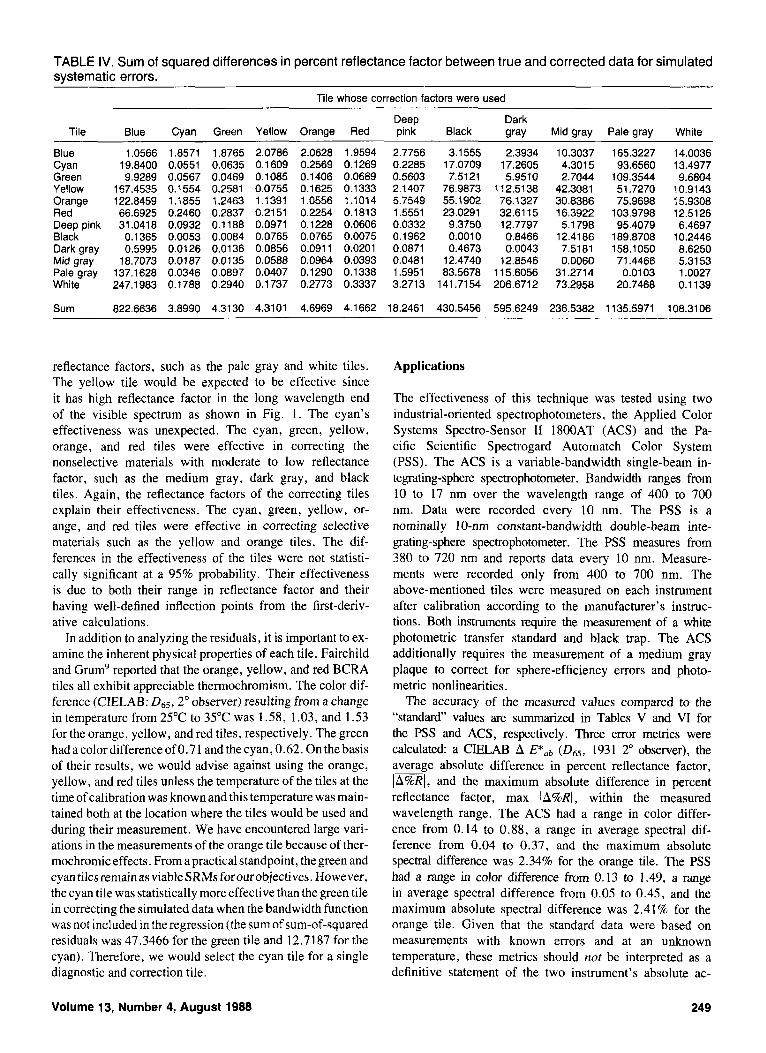
TABLE IV. Sum of squared differences in percent reflectance factor between true and corrected data for simulated systematic errors.

Tile whose correction factors were used

Deep Dark Tile Blue Cyan Green Yellow Orange Red pink Black gray Mid gray Pale gray White

Blue Cyan Green Yellow Orange Red Deep pink Black Dark gray Mid gray Pale gray White

Sum

1.0566 19.8400 9.9289

167.4535 122.8459 66.6925 31.0418 0.1365 0.5995

18.7073 137.1628 247.1983

1 .8571 0.0551 0.0567 0.1554 1.1855 0.2460 0.0932 0.0053 0.01 26 0.0187 0.0346 0.1788

1.8765 0.0635 0.0469 0.2581 1.2463 0.2837 0.1188 0.0084 0.0136 0.0135 0.0897 0.2940

2.0786 0.1 609 0.1085 0.0755 1.1391 0.21 51 0.0971 0.0765 0.0856 0.0588 0.0407 0.1 737

2.0628 1.9594 0.2569 0.1 269 0.1406 0.0689 0.1625 0.1333 1.0556 1.1014 0.2254 0.1813 0.1228 0.0606 0.0765 0.0075 0.091 1 0.0201 0.0964 0.0393 0.1290 0.1338 0.2773 0.3337

822.6636 3.8990 4.31 30 4.31 01 4.6969 4.1 662

2.7756 0.2285 0.5603 2.1407 5.7549 1.5551 0.0332 0.1962 0.0871 0.0481 1.5951 3.2713

18.2461

3.1555 17.0709 7.5121

76.9873 55.1 902 23.0291 9.3750 0.0010 0.4673

12.4740 83.5678

141.71 54

2.3934 17.2605 5.9510

112.5138 76.1327 32.61 15 12.7797 0.8466 0.0043

12.8546 115.6056 206.6712

10.3037 4.301 5 2.7044

42.3081 30.8386 16.3922 5.1 798

12.41 86 7.5181 0.0060

31.2714 73.2958

430.5456 595.6249 236.5382

165.3227 93.6560

109.3544 51.7270 75.9698

103.9798 95.4079

189.8708 1 58.1050 71.4466 0.0103

20.7468

1135.5971

14.0036 13.4977 9.6804

10.9143 15.9308 12.51 26 6.4697

10.2446 8.6250 5.31 53 1.0027 0.1139

108.3106

reflectance factors, such as the pale gray and white tiles. The yellow tile would be expected to be effective since it has high reflectance factor in the long wavelength end of the visible spectrum as shown in Fig. 1. The cyan's effectiveness was unexpected. The cyan, green, yellow, orange, and red tiles were effective in correcting the nonselective materials with moderate to low reflectance factor, such as the medium gray, dark gray, and black tiles. Again, the reflectance factors of the correcting tiles explain their effectiveness. The cyan, green, yellow, orange, and red tiles were effective in correcting selective materials such as the yellow and orange tiles. The differences in the effectiveness of the tiles were not statistically significant at a 95% probability. Their effectiveness is due to both their range in reflectance factor and their having well-defined inflection points from the first-derivative calculations.

In addition to analyzing the residuals, it is important to ex- amine the inherent physical properties of each tile. Fairchild and Grum' reported that the orange, yellow, and red BCRA tiles all exhibit appreciable thermochromism. The color difference (CIELAB: D65, 2" observer) resulting from a change in temperature from 25°C to 35°C was 1.58, 1.03, and 1.53 for the orange, yellow, and red tiles, respectively. The green hadacolordifferenceof0.71 andthecyan, 0.62. Onthebasis of their results, we would advise against using the orange, yellow, and red tiles unless the temperature of the tiles at the time of calibration was known and this temperature was maintained both at the location where the tiles would be used and during their measurement. We have encountered large vari- ations in the measurements of the orange tile because of thermochromic effects. From a practical standpoint, the green and cyan tiles remain as viable SRMs forourobjectives. However, the cyan tile was statistically more effective than the green tile in correcting the simulated data when the bandwidth function was not included in the regression (the sum of sum-of-squared residuals was 47.3466 for the green tile and 12.7187 for the cyan). Therefore, we would select the cyan tile for a single diagnostic and correction tile.

Applications

The effectiveness of this technique was tested using two industrial-oriented spectrophotometers, the Applied Color Systems Spectro-Sensor I1 1800AT (ACS) and the Pa- cific Scientific Spectrogard Automatch Color System (PSS). The ACS is a variable-bandwidth single-beam integrating-sphere spectrophotometer. Bandwidth ranges from 10 to 17 nm over the wavelength range of 400 to 700 nm. Data were recorded every 10 nm. The PSS is a nominally 10-nm constant-bandwidth double-beam integrating-sphere spectrophotometer. The PSS measures from 380 to 720 nm and reports data every 10 nm. Measure- ments were recorded only from 400 to 700 nm. The above-mentioned tiles were measured on each instrument after calibration according to the manufacturer's instruc- tions. Both instruments require the measurement of a white photometric transfer standard and black trap. The ACS additionally requires the measurement of a medium gray plaque to correct for sphere-efficiency errors and photometric nonlinearities.

The accuracy of the measured values compared to the "standard" values are summarized in Tables V and VI for the PSS and ACS, respectively. Three error metrics were calculated: a CIELAB A E*ab (D65, 1931 2" observer), the average absolute difference in percent reflectance factor, ImI, and the maximum absolute difference in percent reflectance factor, max (A%R(, within the measured wavelength range. The ACS had a range in color difference from 0.14 to 0.88, a range in average spectral difference from 0.04 to 0.37, and the maximum absolute spectral difference was 2.34% for the orange tile. The PSS had a range in color difference from 0.13 to 1.49, a range in average spectral difference from 0.05 to 0.45, and the maximum absolute spectral difference was 2.41% for the orange tile. Given that the standard data were based on measurements with known errors and at an unknown temperature, these metrics should not be interpreted as a definitive statement of the two instrument's absolute ac-


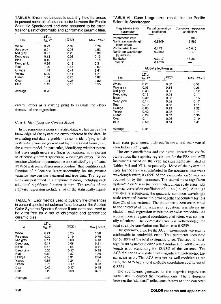
TABLE V. Error metrics used to quantify the differences in percent spectral reflectance factor between the Pacific Scientific Spectrogard and data assumed to be error- free for a set of chromatic and achromatic ceramic tiles.

Tile Max I A%R 1 White Pale gray Mid gray Deep gray Black Deep pink Red Orange Yellow Green Cyan Blue

Average

0.22 0.21 0.27 0.13 0.45 0.66 1.29 1.49 0.99 1.04 1.14 1.19

0.76

0.39 0.38 0.25 0.05 0.13 0.16 0.45 0.41 0.41 0.25 0.25 0.18

0.76 0.53 0.30 0.13 0.18 0.31 2.07 2.41 1.71 0.67 0.82 0.55

curacy, rather as a starting point to evaluate the effectiveness of the regressions.

Case I : Identifiing the Correct Model

In the regressions using simulated data, we had an apriori knowledge of the systematic errors inherent in the data. In evaluating real data, a problem exists in identifying which systematic errors are present and their functional forms, i.e., the correct model. In particular, identifying whether potential wavelength errors are linear or nonlinear is important to effectively correct systematic wavelength errors. To determine which error parameters were statistically significant, we used a stepwise regression procedure6 that identifies each function of reflectance factor accounting for the greatest variance between the measured and true data. The regressions are performed in a stepwise fashion, including each additional significant function in turn. The results of the stepwise regression include a list of the statistically signif-

TABLE VI. Error metrics used to quantify the differences in percent spectral reflectance factor between the Applied Color Systems Spectro-Sensor II and data assumed to be error-free for a set of chromatic and achromatic ceramic tiles.

A F a b Tile DS5, 2” /rnJ Max I A%R 1

White 0.21 0.23 1.28 Pale gray 0.20 0.19 0.79 Mid gray 0.14 0.08 0.16 Deep gray 0.17 0.08 0.21 Black 0.18 0.04 0.1 1 Deep pink 0.30 0.17 0.49 Red 0.80 0.37 1.80 Orange 0.59 0.31 2.34 Yellow 0.88 0.24 1.31 Green 0.75 0.17 0.70 Cyan 0.49 0.17 0.45 Blue 0.22 0.09 0.81

Average 0.41

TABLE VII. Case I regression results for the Pacific Scientific Spectrogard.

Regression error Partial correlation Corrective regression parameter coefficient coefficient

Photometric zero - 0.086 Nonlinear wavelength 0.8309 2.589

Photometric linear 0.143 - 0.01 0 Nonlinear wavelength 0.01 02 -0.179

Bandwidth 0.0017 - 16.360

(sine wave)

(quadratic)

Total R2 0.9859 - Model effectiveness

Tile Max I A%R 1 White Pale gray Mid gray Deep gray Black Deep pink Red Orange Yellow Green Cyan Blue

Average

0.23 0.09 0.08 0.13 0.30 0.14 0.70 0.65 0.42 0.29 0.1 1 0.59

0.31

0.30 0.14 0.08 0.04 0.08 0.05 0.33 0.23 0.35 0.07 0.03 0.14

0.56 0.26 0.12 0.1 1 0.13 0.17 1.15 1.25 0.71 0.30 0.10 0.41

icant error parameters, their coefficients, and their partial correlation coefficients.

The error coefficients and the partial correlation coefficients from the stepwise regressions for the PSS and ACS instruments based on the cyan measurements are listed in Tables VII and VIII, respectively. Most of the systematic error for the PSS was attributed to the nonlinear sine-wave wavelength error; 83.09% of the systematic error was accounted for by this parameter. The second-most-significant systematic error was the photometric linear scale error with a partial correlation coefficient of 0.143 (14.3%). Although statistically significant, the quadratic nonlinear wavelength scale error and bandwidth error together accounted for less than 2% of the variance. The photometric zero error, equal to the intercept of the regression equation, was always included in each regression within the stepwise procedure. As a consequence, a partial correlation coefficient was not usually calculated. The systematic error was well-modeled; the total multiple correlation coefficient was 0.9859.

The systematic error for the ACS measurements was mainly attributable to bandwidth error. This parameter accounted for 57.88% of the total systematic error. The second-most- significant systematic error was a nonlinear quadratic wavelength error accounting for 18.93% of the variance. The ACS did not have a statistically significant photometric linear scale error. The ACS was not as well-modeled as the PSS; the ACS had a total multiple correlation coefficient of 0.8221.

The coefficients generated in the stepwise regressions were used to correct the measurements. The differences between the “standard” reflectance factors and the corrected


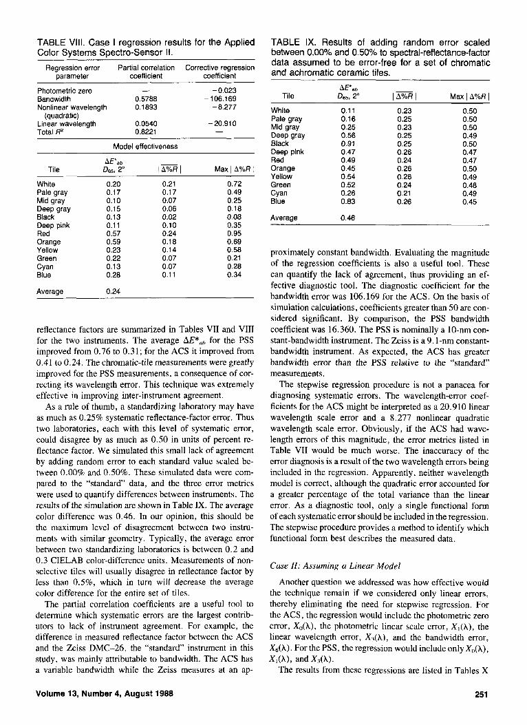
TABLE VIII. Case I regression results for the Applied Color Systems Spectro-Sensor I I .


Photometric zero - -0.023 Bandwidth 0.5788 -106.169 Nonlinear wavelength 0.1893 - 8.277

Linear wavelength 0.0540 - 20.91 0 Total RZ 0.8221 -

(quadratic)

__ ______~

Model effectiveness

Tile I r n I Max I A%R 1


Average

0.20 0.17 0.10 0.15 0.13 0.1 1 0.57 0.59 0.23 0.22 0.13 0.28

0.24

0.21 0.17 0.07 0.06 0.02 0.10 0.24 0.18 0.14 0.07 0.07 0.1 1

0.72 0.49 0.25 0.18 0.08 0.35 0.95 0.69 0.58 0.21 0.28 0.34

reflectance factors are summarized in Tables VII and VIII for the two instruments. The average for the PSS improved from 0.76 to 0.31; for the ACS it improved from 0.41 to 0.24. The chromatic-tile measurements were greatly improved for the PSS measurements, a consequence of correcting its wavelength error. This technique was extremely effective in improving inter-instrument agreement.

As a rule of thumb, a standardizing laboratory may have as much as 0.25% systematic reflectance-factor error. Thus two laboratories, each with this level of systematic error, could disagree by as much as 0.50 in units of percent reflectance factor. We simulated this small lack of agreement by adding random error to each standard value scaled between 0.00% and 0.50%. These simulated data were compared to the “standard” data, and the three error metrics were used to quantify differences between instruments. The results of the simulation are shown in Table IX. The average color difference was 0.46. In our opinion, this should be the maximum level of disagreement between two instruments with similar geometry. Typically, the average error between two standardizing laboratories is between 0.2 and 0.3 CIELAB color-difference units. Measurements of nonselective tiles will usually disagree in reflectance factor by less than 0.5%, which in turn will decrease the average color difference for the entire set of tiles.

The partial correlation coefficients are a useful tool to determine which systematic errors are the largest contrib- utors to lack of instrument agreement. For example, the difference in measured reflectance factor between the ACS and the Zeiss DMC-26, the “standard” instrument in this study, was mainly attributable to bandwidth. The ACS has a variable bandwidth while the Zeiss measures at an ap-

TABLE IX. Results of adding random error scaled between 0.000/0 and 0.50% to spectral-reflectance-factor data assumed to be error-free for a set of chromatic and achromatic ceramic tiles.

Tile Max I A%R I White Pale gray Mid gray Deep gray Black Deep pink Red Orange Yellow Green Cyan Blue

0.1 1 0.16 0.25 0.56 0.91 0.47 0.49 0.45 0.54 0.52 0.26 0.83

0.23 0.25 0.23 0.25 0.25 0.26 0.24 0.26 0.26 0.24 0.21 0.26

0.50 0.50 0.50 0.49 0.50 0.47 0.47 0.50 0.49 0.48 0.49 0.45

Average 0.46

proximately constant bandwidth. Evaluating the magnitude of the regression coefficients is also a useful tool. These can quantify the lack of agreement, thus providing an effective diagnostic tool. The diagnostic coefficient for the bandwidth error was 106.169 for the ACS. On the basis of simulation calculations, coefficients greater than 50 are considered significant. By comparison, the PSS bandwidth coefficient was 16.360. The PSS is nominally a 10-nm constant-bandwidth instrument. The Zeiss is a 9. l-nm constant- bandwidth instrument. As expected, the ACS has greater bandwidth error than the PSS relative to the “standard” measurements.

The stepwise regression procedure is not a panacea for diagnosing systematic errors. The wavelength-error coefficients for the ACS might be interpreted as a 20.910 linear wavelength scale error and a 8.277 nonlinear quadratic wavelength scale error. Obviously, if the ACS had wavelength errors of this magnitude, the error metrics listed in Table VII would be much worse. The inaccuracy of the error diagnosis is a result of the two wavelength errors being included in the regression. Apparently, neither wavelength model is correct, although the quadratic error accounted for a greater percentage of the total variance than the linear error. As a diagnostic tool, only a single functional form of each systematic error should be included in the regression. The stepwise procedure provides a method to identify which functional form best describes the measured data.

Case !I: Assuming a Linear Model

Another question we addressed was how effective would the technique remain if we considered only linear errors, thereby eliminating the need for stepwise regression. For the ACS, the regression would include the photometric zero error, Xo(h), the photometric linear scale error, X,(h) , the linear wavelength error, X3(h), and the bandwidth error, X&). For the PSS, the regression would include only Xo(h), X W , and X d M .

The results from these regressions are listed in Tables X


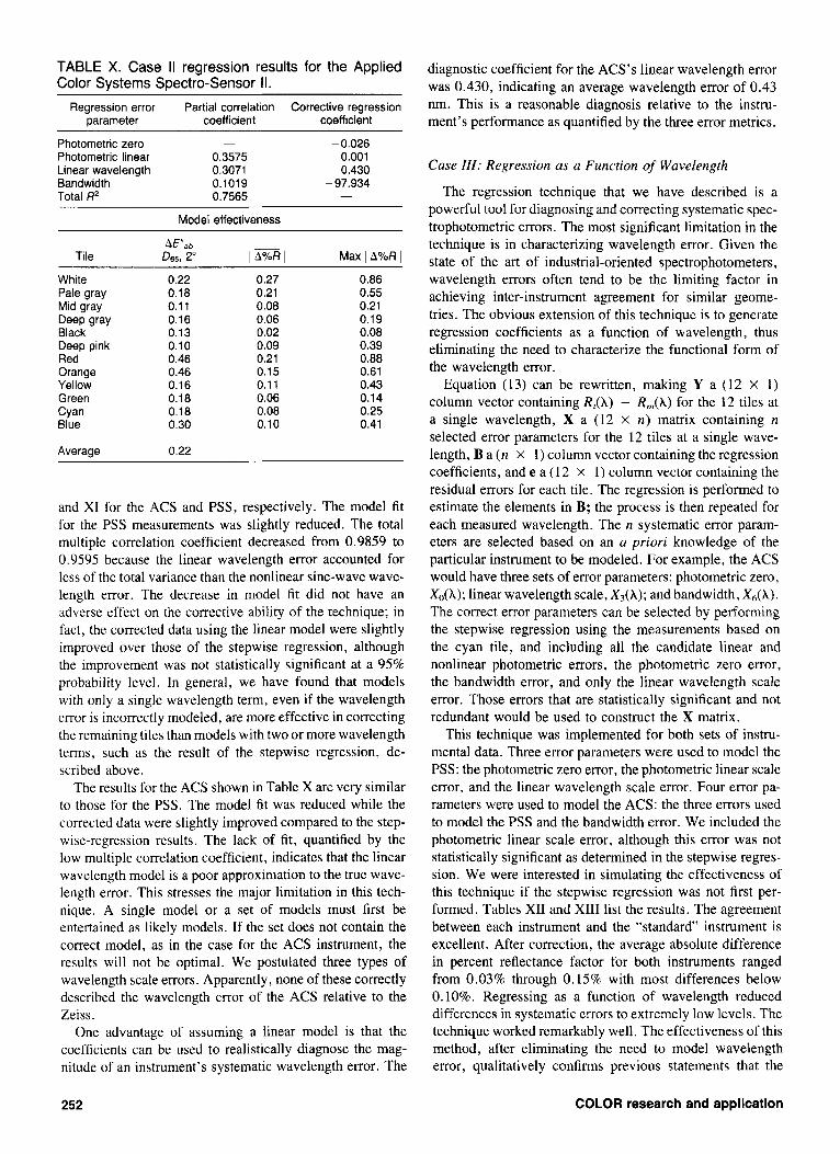
TABLE X. Case II regression results for the Applied Color Systems Spectro-Sensor 11.


- 0.026 Photometric zero -

Photometric linear 0.3575 0.001 Linear wavelength 0.3071 0.430 Bandwidth 0.1019 - 97.934 Total R2 0.7565 -

Model effectiveness

Tile


A F a b

D65, 2"

0.22 0.18 0.1 1 0.16 0.13 0.10 0.46 0.46 0.16 0.18 0.18 0.30

Average 0.22

I & % 0.27 0.21 0.08 0.06 0.02 0.09 0.21 0.15 0.1 1 0.06 0.08 0.10

Max I AYoR I 0.86 0.55 0.21 0.19 0.08 0.39 0.88 0.61 0.43 0.14 0.25 0.41

and XI for the ACS and PSS, respectively. The model fit for the PSS measurements was slightly reduced. The total multiple correlation coefficient decreased from 0.9859 to 0.9595 because the linear wavelength error accounted for less of the total variance than the nonlinear sine-wave wavelength error. The decrease in model fit did not have an adverse effect on the corrective ability of the technique; in fact, the corrected data using the linear model were slightly improved over those of the stepwise regression, although the improvement was not statistically significant at a 95% probability level. In general, we have found that models with only a single wavelength term, even if the wavelength error is incorrectly modeled, are more effective in correcting the remaining tiles than models with two or more wavelength terms, such as the result of the stepwise regression, described above.

The results for the ACS shown in Table X are very similar to those for the PSS. The model fit was reduced while the corrected data were slightly improved compared to the stepwise-regression results. The lack of fit, quantified by the low multiple correlation coefficient, indicates that the linear wavelength model is a poor approximation to the true wavelength error. This stresses the major limitation in this technique. A single model or a set of models must first be entertained as likely models. If the set does not contain the correct model, as in the case for the ACS instrument, the results will not be optimal. We postulated three types of wavelength scale errors. Apparently, none of these correctly described the wavelength error of the ACS relative to the Zeiss.

One advantage of assuming a linear model is that the coefficients can be used to realistically diagnose the magnitude of an instrument's systematic wavelength error. The

diagnostic coefficient for the ACS's linear wavelength error was 0.430, indicating an average wavelength error of 0.43 nm. This is a reasonable diagnosis relative to the instrument's performance as quantified by the three error metrics.

Case III : Regression as a Function of Wavelength

The regression technique that we have described is a powerful tool for diagnosing and correcting systematic spectrophotometric errors. The most significant limitation in the technique is in characterizing wavelength error. Given the state of the art of industrial-oriented spectrophotometers, wavelength errors often tend to be the limiting factor in achieving inter-instrument agreement for similar geome- tries. The obvious extension of this technique is to generate regression coefficients as a function of wavelength, thus eliminating the need to characterize the functional form of the wavelength error.

Equation (13) can be rewritten, making Y a (12 X 1) column vector containing R,(X) - R,(A) for the 12 tiles at a single wavelength, X a (12 x n ) matrix containing n selected error parameters for the 12 tiles at a single wavelength, B a ( n X 1 ) column vector containing the regression coefficients, and e a ( I 2 X I ) column vector containing the residual errors for each tile. The regression is performed to estimate the elements in B; the process is then repeated for each measured wavelength. The n systematic error parameters are selected based on an a priori knowledge of the particular instrument to be modeled. For example, the ACS would have three sets of error parameters: photometric zero, X&); linear wavelength scale, X,(h); and bandwidth, X,(X). The correct error parameters can be selected by performing the stepwise regression using the measurements based on the cyan tile, and including all the candidate linear and nonlinear photometric errors, the photometric zero error, the bandwidth error, and only the linear wavelength scale error. Those errors that are statistically significant and not redundant would be used to construct the X matrix.

This technique was implemented for both sets of instrumental data. Three error parameters were used to model the PSS: the photometric zero error, the photometric linear scale error, and the linear wavelength scale error. Four error parameters were used to model the ACS: the three errors used to model the PSS and the bandwidth error. We included the photometric linear scale error, although this error was not statistically significant as determined in the stepwise regression. We were interested in simulating the effectiveness of this technique if the stepwise regression was not first performed. Tables XI1 and XI11 list the results. The agreement between each instrument and the "standard" instrument is excellent. After correction, the average absolute difference in percent reflectance factor for both instruments ranged from 0.03% through 0.15% with most differences below 0.10%. Regressing as a function of wavelength reduced differences in systematic errors to extremely low levels. The technique worked remarkably well. The effectiveness of this method, after eliminating the need to model wavelength error, qualitatively confirms previous statements that the


TABLE XI. Case II regression results for the Pacific Scientific Spectrogard.


Photometric zero - 0.047 Photometric linear 0.1518 - 0.009 Linear wavelength 0.8077 1.209 Total RZ 0.9595 -

~ ~

Model effectiveness

Tile Max I A%R I White Pale gray Mid gray Deep gray Black Deep pink Red Orange Yellow Green Cyan Blue

Average

0.21 0.07 0.08 0.1 1 0.42 0.09 0.58 0.48 0.42 0.25 0.08 0.68

0.29

0.24 0.1 1 0.07 0.03 0.12 0.04 0.32 0.20 0.30 0.06 0.04 0.16

0.48 0.22 0.16 0.08 0.17 0.10 0.98 0.84 0.69 0.27 0.24 0.36

limiting factor in achieving reasonable inter-instrument agreement is wavelength error.

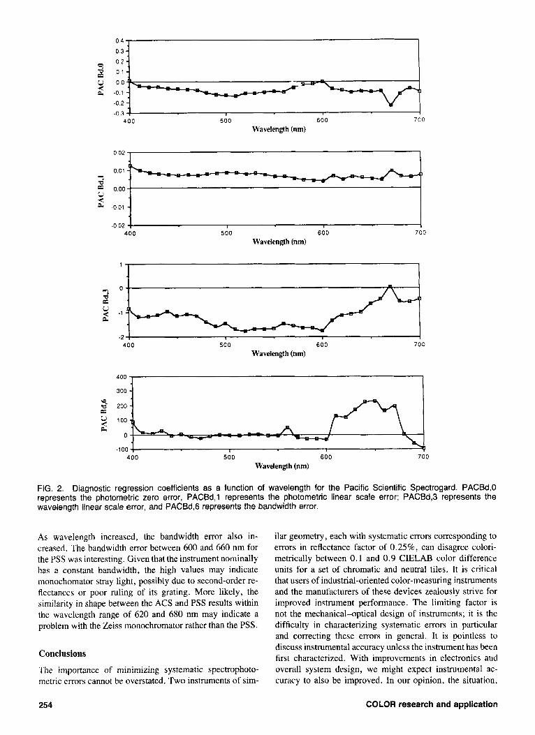
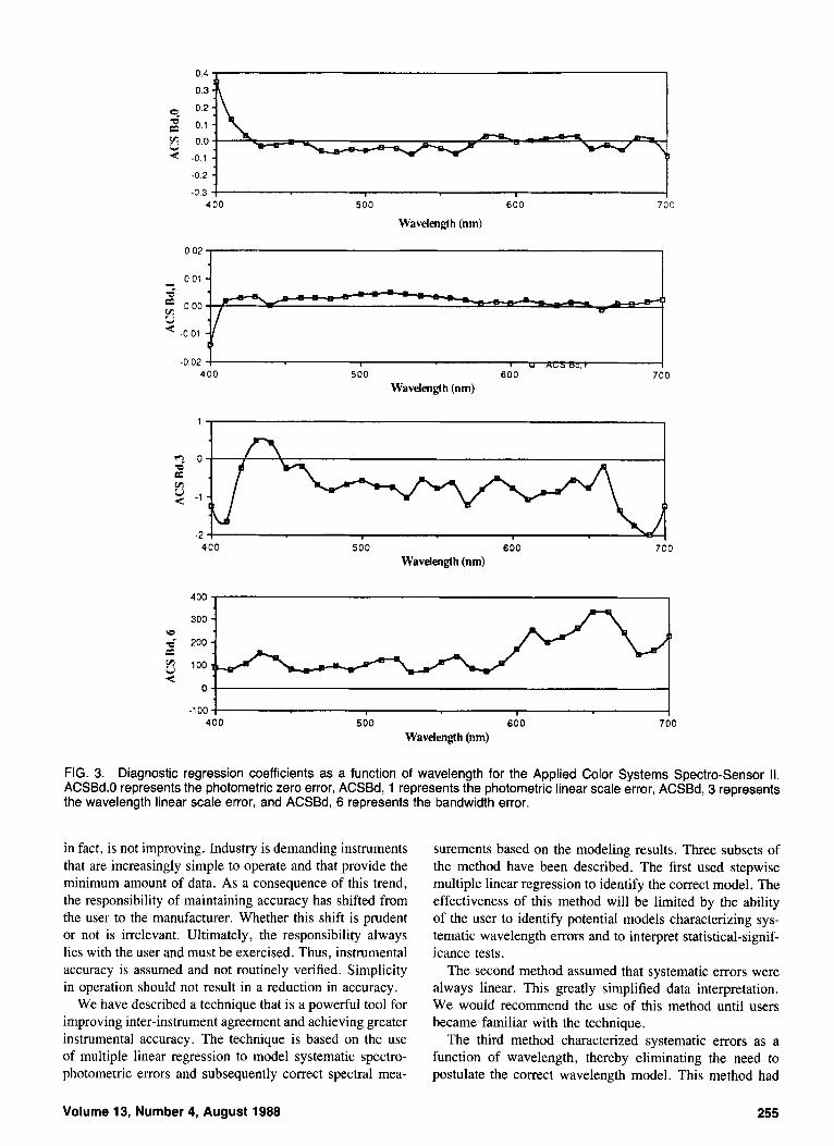
Regressing as a function of wavelength has also yielded an excellent purview of each instrument's systematic errors. The diagnostic regression coefficients for the PSS and the ACS are plotted in Figs. 2 and 3, respectively. Both instruments have small negative photometric zero errors sug- gesting that the reference measurements were based on cal- ibrations with a black trap with a finite reflectance factor or with input-optics stray light. At 400 and 410 nm, the ACS has a positive zero error that is probably due to a reduced signal-to-noise ratio attributable to low detector response at the short-wavelength end of the visible spectrum.

Both instruments had negligible photometric linear scale

TABLE XII. Case Ill regression results for the Pacific Scientific Spectrogard. The regression model included the following systematic errors as a function of wavelength: photometric zero, X&); photometric linear, X,(X); and linear wavelength, X&).

A F a b Tile Dss, 2" IP%RI Max I A%R 1

White 0.09 0.08 0.20 Pale gray 0.13 0.09 0.20 Mid gray 0.19 0.15 0.21 Deep gray 0.24 0.05 0.1 1 Black 0.43 0.07 0.18 Deep pink 0.18 0.09 0.24 Red 0.29 0.08 0.21 Orange 0.06 0.05 0.40 Yellow 0.20 0.06 0.23 Green 0.14 0.05 0.10 Cyan 0.1 1 0.03 0.10 Blue 0.54 0.10 0.19

Average 0.22

TABLE XIII. Case regression results for the Applied Color Systems Spectro-Sensor II. The regression model included the following systematic errors as a function of wavelength: photometric zero, X&); photometric linear, X , (X); linear wavelength, X,(X); and bandwidth, X&.

AE*ab D65, 2" JmI Max I A%R I Tile

White 0.07 0.07 0.15 Pale gray 0.10 0.07 0.17 Mid gray 0.06 0.04 0.25 Deep gray 0.27 0.06 0.1 4 Black 0.36 0.05 0.19 Deep pink 0.13 0.05 0.22 Red 0.04 0.05 0.18 Orange 0.13 0.05 0.22 Yellow 0.12 0.08 0.21 Green 0.05 0.05 0.23 Cyan 0.28 0.09 0.28 Blue 0.26 0.05 0.13

Average 0.16

errors, except at 400 nm for the ACS: The white transfer standard for the ACS is a porcelain enamel tile; near 400 nm, its reflectance factor decreases sharply. As a consequence, reflectance factors greater than that of the transfer standard have slightly greater uncertainty. This, combined with the decrease in detector responsivity, increased the photometric error. The standard measurements were calibrated relative to barium sulfate. It is important to have white standards with reflectance factors near 100% across the spectral region of interest.

The wavelength error for the PSS was, on average, - 1.18, which agrees well with the calculated average linear wavelength error based on the measurement of only the cyan tile. The shape of the wavelength-error curve does not support the results of the stepwise regression, which identified a sine wave as the best wavelength model. This discrepancy is probably a result of using 12 tiles to characterize the wavelength error rather than just the cyan tile. We should recall that the wavelength error is modeled based on the first derivative of the reflectance-factor measurements. The more inflection points a tile has, the greater the accuracy in characterizing the systematic wavelength error. The cyan tile has only a single inflection point between 400 and 700 nm. Excluding the nonselective tiles, there are eight well- defined inflection points for the selective tiles. Certainly, the wavelength error, as characterized by Fig. 2, is a more accurate description of the PSS wavelength error. The wavelength error at 670 nm possibly indicates either a measurement error, a recording error, or an analog-to-digital transfer error. The wavelength error for the ACS was on average -0.75, which also agrees with the result from the linear model based on the cyan-tile measurement. The shape of the wavelength error curve qualitatively seems to be random, which explains why none of the wavelength models accounted for much of the measurement variability in the regressions.

The bandwidth error curve for the ACS was as expected.


0 4

03 0 2

?.

u 0 0

2 0 1

2 - 0 1

-0 2 -0 3

400 500 600 700

Wavelength (nm)

a -001

-0.02 , I I

400 500 600 700

Wavelength (nm)

J I

y -1 a O 2

-c I

400 500 600 700 Wavelength (nm)

400

300

2 200

y 100 cc

a 0

-100 400 500 600 700

Wavelength (nm)

FIG. 2. Diagnostic regression coefficients as a function of wavelength for the Pacific Scientific Spectrogard. PACBd,O represents the photometric zero error, PACBd,l represents the photometric linear scale error; PACBd,3 represents the wavelength linear scale error, and PACBd,G represents the bandwidth error.

As wavelength increased, the bandwidth error also increased. The bandwidth error between 600 and 660 nm for the PSS was interesting. Given that the instrument nominally has a constant bandwidth, the high values may indicate monochomator stray light, possibly due to second-order re- flectances or poor ruling of its grating. More likely, the similarity in shape between the ACS and PSS results within the wavelength range of 620 and 680 nm may indicate a problem with the Zeiss monochromator rather than the PSS.

Conclusions

The importance of minimizing systematic spectrophotometric errors cannot be overstated. Two instruments of sim-

ilar geometry, each with systematic errors corresponding to errors in reflectance factor of 0.25%, can disagree colori- metrically between 0.1 and 0.9 CIELAB color difference units for a set of chromatic and neutral tiles. It is critical that users of industrial-oriented color-measuring instruments and the manufacturers of these devices zealously strive for improved instrument performance. The limiting factor is not the mechanical-optical design of instruments; it is the difficulty in characterizing systematic errors in particular and correcting these errors in general. It is pointless to discuss instrumental accuracy unless the instrument has been first characterized. With improvements in electronics and overall system design, we might expect instrumental accuracy to also be improved. In our opinion, the situation,


0.4

0.3

0.2

0.1

0.0

-0.1

-0 2

-0 3 400 500 600 700

Wavelength (nm)

0 02

0 01 - -6- = 0 0 0 5

-001

-0 02 400 500 600 700

Wavelength (nm)

1

2 0

y -1

cf (I:

-2 400 500 600

Wavelength (nm) 700

400

300

200

100

0

-1 00 400 500 600 700

Wavelength (nm)

FIG. 3. Diagnostic regression coefficients as a function of wavelength for the Applied Color Systems Spectro-Sensor II. ACSBd,O represents the photometric zero error, ACSBd, 1 represents the photometric linear scale error, ACSBd, 3 represents the wavelength linear scale error, and ACSBd, 6 represents the bandwidth error.

in fact, is not improving. Industry is demanding instruments that are increasingly simple to operate and that provide the minimum amount of data. As a consequence of this trend, the responsibility of maintaining accuracy has shifted from the user to the manufacturer. Whether this shift is prudent or not is irrelevant. Ultimately, the responsibility always lies with the user and must be exercised. Thus, instrumental accuracy is assumed and not routinely verified. Simplicity in operation should not result in a reduction in accuracy.

We have described a technique that is a powerful tool for improving inter-instrument agreement and achieving greater instrumental accuracy. The technique is based on the use of multiple linear regression to model systematic spectrophotometric errors and subsequently correct spectral mea-

surements based on the modeling results. Three subsets of the method have been described. The first used stepwise multiple linear regression to identify the correct model. The effectiveness of this method will be limited by the ability of the user to identify potential models characterizing systematic wavelength errors and to interpret statistical-significance tests.

The second method assumed that systematic errors were always linear. This greatly simplified data interpretation. We would recommend the use of this method until users became familiar with the technique.

The third method characterized systematic errors as a function of wavelength, thereby eliminating the need to postulate the correct wavelength model. This method had


the greatest effectiveness as both a diagnostic and a corrective tool. The application of this method brought two instruments with similar geometry into close agreement in spectral reflectance factor, within the total uncertainty of standardizing laboratories.

The following outlines how the first method can be implemented in an industrial environment. The first step is to obtain a set of calibrated chromatic and neutral tiles or filters. The calibration should be for the same geometry as for the measurements. For example, in this article we considered total reflectance-factor measurements. The three instruments all had integrating spheres and were set up to measure total reflectance factor. Calibration data based on integrating-sphere instruments should not be used to diagnose errors in a 4.90 instrument and vice versa. Geometry is particularly important if the standard reference materials are glossy, such as the BCRA Series I1 tiles. Transmittance measurements should be corrected based on filter calibra- tions. Systematic errors characterized using transmittance measurements often are used to correct reflectance-factor measurements. The reverse case usually is not applied since stray-light errors due to entrance optics, such as an integrating sphere, do not apply to transmittance measurements. Certainly, wavelength corrections based on reflectance-factor measurements can be applied to transmittance measurements. The second step is to measure each tile and calculate the various functions of reflectance factor for the cyan tile. Third, these functions are entered into a stepwise multiple linear regression program. There are many general-purpose statistics packages containing stepwise regression that run on personal computers, minicomputers, or main-frame computers. Based on an analysis of variance, the fourth step is to select those errors that are statistically significant and not redundant. Fifth, one corrects all the measured data and evaluates the improvement in reflectance factors and color differences. It is important to have samples with known reflectance factors that are used to evaluate the effectiveness of the technique. By definition, the measurements of the

cyan tile will agree more closely to the calibration values. If the agreement for the other tiles is not universally improved, the model must be considered suspect.

In our laboratory, we are using this technique to improve our instrumental accuracy relative to the United States Na- tional Bureau of Standards for 45/0 measurements and to track instrument performance over time. We plot the regression coefficients for the cyan tile each time an instrument is used, in addition to other pertinent information such as ambient temperature and the operator. Very quickly we can diagnose the performance of our instruments with quanti- tative data that relate directly to systematic errors. We have found this technique much more effective in diagnosing photometric and wavelength errors than evaluating colorimetric data or reflectance-factor data at specific wavelengths. In addition, this has reduced the time required to diagnose instrument performance.

1. Standard Dejnitions of Terms Relating to Appearance of Materials, ASTM Designation: E284, American Society for Testing and Materials, Philadelphia.

2. E. C. Carter and F. W. Billmeyer, Jr., Material standards and their use in color measurement, Color Res. Appl. 4, 96-100 (1979).

3. F. W. Billmeyer, Jr., and P. J. Alessi, Assessment of color-measuring instruments, Color Rer. Appl . 6, 195-203 (1981).

4. K. H. Petersen, An Investigation of New Methods to Improve the Ac- curacy of Some Modern Color Spectrophotometers, Master of Science thesis in progress, Rochester Institute of Technology, 1987.

5. A. R. Robertson, “Diagnostic Performance Evaluation of Spectropho- tometers,” presented at Advances in Standurds and Methodology in Spectrophotometry, Oxford, England, 1986.

6. N. R. Draper and H. Smith, Applied Regression Analysis, 2nd. ed. . John Wiley & Sons, New York, 1981.

7 . Cerumic Colour Standards Manual, Series 11, British Ceramic Research Association, Stoke-on-Trent, England, 1984.

8. Yoneda Glass Bead Co., Ltd., Osaka, Japan. 9. M. D. Fairchild and F. Grum, Thermochromism of ceramic reference

tiles, Appl. Opt. 24, 3432-3433 (1985).

Received July 5 , 1987; accepted September 20, 1987


empirical modeling of systematic spectrophotometric errors

Documents