determinants of economic growth: u.s., japan, china ... · 1 determinants of economic growth: u.s.,...

1

Determinants of Economic Growth:

U.S., Japan, China, Singapore and Indonesia

Effendy Juraimin California State University, Hayward

Empirical findings from 1980 to 1995 show that China, Japan, Singapore, and Indonesia have different economic growth models than that of United States. For example, one experiment indicates that the trade effect on growth is significantly different between China and U.S. The fact that each country has different dominant determinants of growth supports the notion that they have different economic growth models. Higher secondary level enrollment and terms of trade deterioration enhances growth of U.S, with the secondary level enrollment as the biggest factor. Whereas Japan has higher secondary level enrollment and lower inflation rate as key growth factors, predominantly the secondary level enrollment. Growth of China is stimulated by higher saving rate, lower inflation rate, and terms of trade improvement, but the saving rate plays the biggest role. Higher life expectancy and saving rate mostly explain growth of Singapore, especially the life expectancy. At last, higher government consumption ratio and lower life expectancy equally explains the growth of Indonesia.

I. Introduction

At the height of Asian economic crisis in 1997, International Monetary Fund (IMF)

arrived on the scene in Indonesia to approve a $10 billion bailout package that tied to

economic reform measures. The reform required budget cut, tight credit, high interest rates,

and bank closings; in order to lower inflation, end weakening currency, and stop foreign

exchange loss. These solutions were similar to the countries that IMF typically faced, but

the problems were very different. The government of those countries spent beyond its

2

means, and financed the budget deficits by printing money through its central bank. The

results were high inflation, weakening currency, and loss of foreign exchange reserve.

In contrary, Indonesia had budget surplus, inflation was low, and foreign exchange

reserves were stable. Instead of restoring public confidence, the IMF remedies caused bank

panic and economic meltdown. The closure of 16 insolvent banks in November 1997 set

off $2 billion withdrawal from two third of all the country’s bank. The tight monetary and

fiscal policies deprived businesses from bank loans and government funds that were

necessary to avoid mass unemployment and bankruptcies. The whole economy eventually

shrank by 13.7 percent in 1998, from an averaged 7 percent growth in previous 25 years.

This economic blunder1 raises the following key question. Does each country at

different development stage, with different social choices, and different economic

structure, respond similarly to reform policies to promote economic growth? In other

words, does each country with different social and economic characters have a similar

economic growth model? If the answer is yes, policy makers should shape their economic

policies according to their condition, and international agencies, such as IMF and World

Bank, should formulate reform strategies accordingly.

We attempt to answer the above question by comparing economic growth models

of four distinctive countries against the United States (U.S.). If they indeed have different

economic growth models, what are key determinants of their corresponding economic

growths? We select these countries because of their distinctive characteristics.

1 The author does not imply that IMF worsened the crisis, but they could have done better during the early stage of the crisis.

3

United States has the largest real GDP ($9 trillion2) and also one of the highest real

GDP per capita ($ 33,000) in the world. It has total population that ranks fourth globally

(276 million), close to Indonesia’s, and total area of 9.4 million km2 that matches China’s.

Japan’s real GDP ($2.8 trillion) is one third of US’s and half of China’s. But it has real

GDP per capita ($22,000) that is almost six times higher than China’s, and not far behind

from US’s and Singapore’s. Its total population of 127 million people, almost half of US’s,

lives in only 378 thousand km 2 of total area, a twenty five times smaller than US’s. China

is the most populous country in the world (1.3 billion) and occupies a total area (9.6

million km2) that is similar in size to US’s. Its real GDP ($4.9 trillion) is half of US’s, but

the people earn only $3,847 per capita, ten times less than that of US’s. Singapore has a

small economy with $101 million real GDP, but a rich economy with $24,000 per capita. It

also has a small population (4.2 million) and a very small total area (633 km2). Indonesia

is almost a total opposite of Singapore. It is the fifth most populous country with 225

million populations that live in 2 million km2 of total area. It has a bigger economy than

Singapore’s with $598 million of real GDP, but a poorer economy with $2,662 per capita,

almost ten times less than Singapore’s.

The second section of this paper discusses economic growth theories, Neoclassical

and Endogenous, and how does this paper fit into these theories. It also describes how does

it differ from other empirical works in economic growth. The third section explains the

data that is used in the analysis and defines each dependent and independent variables. The

fourth section developed a pooled regression model to test if there is a significant different

between each country’s growth model against the US’. If they are significantly different,

2 All statistics in this paragraph are in year 2000 (source: CountryWatch.com)

4

we will discuss key determinants of their growths that explain the differences. The fifth

section discusses the empirical findings and policy implications, and the sixth section

draws conclusion from this research and suggests potential further research.

II. Economic Growth theories

A. Neoclassical

In the late 1950’s and the 1960’s, economic growth theory is mainly the

neoclassical growth theory developed by Solow (1956), Swan (1956), Cass (1965), and

Koopmans (1965). The theory focuses on capital accumulation and its link to savings

decisions and population growth. It says that increase in the savings rate raises output

growth rate in the short run, but not in the long run. In the long run, economy will reach a

steady state where per capita output is not growing anymore or constant. The key

assumption here is diminishing marginal product of capital. And it applies to population

growth factor as well. Increase in the population growth rate raises an aggregate output

growth rate, but reduces level of output per capita. The theory implies that country with a

lower initial income per capita will eventually catch-up or converge with those of higher

income per capita as long as they have equal savings rate, population growth, and

technology. The paper does not concern with this absolute convergence property of the

theory, but instead it uses the savings rate and population growth variables to explain the

output per capita growth rate of each country.

Neoclassical implies that only technological progress affects per capita output in

the long run. But it does not explain what are determinants of the technological progress.

The technological part is exogenous (i.e. Solow residual), and endogenous growth theory

focuses on the determinants of that part.

5

B. Endogenous

Starting from late 1980s, endogenous becomes a focus of growth theory

development with Romer (1986) and Lucas (1988). The theory looks at how societal

choices affect the technological progress. Specifically, they look at human capital and

more recently social-political institutions. The assumption of the theory, contrarily with

neoclassical, is a constant marginal product of capital. This means that the technology

increases the productivity of capital and labor which allows output per capita to grow

endlessly. Therefore countries with lower income per capita will converge with those of

higher income per capita only if their determinants of technological progress (i.e. human

capital and social-political institutions) are the same. The paper again does not concern

with this conditional convergence property of the theory. Instead it uses the human capital

and the institution variables to explain the output per capita growth rate of each country.

Many empirical studies in endogeneous growth, namely Barro (1991), Barro and

Sala-i-Martin (1992), Barro (1996), perform a cross section analysis across various

countries and mainly concern with conditional convergence issue. Whereas this paper

performs a pooled regression analysis that combines thirty years time series with five cross

sectional countries (as dummy variables), and only concerns with comparison of growth

models. But it uses some of Barro’s endogenous variables for our growth model. Equation

(1) is an example of Barro’s growth equation in a complete form (see Barro 1996).

Per Capita growth rate = log (initial GDP) + initial male secondary and higher schooling + log(initial life

expectancy) + log(initial GDP)*male schooling + log(fertility rate) + government consumption ratio + rule-

of-law index + terms-of-trade change + democracy index + democracy index squared + inflation rate + Sub

Saharan Africa dummy + Latin America dummy + East Asia dummy ............................................... (1)

Next section defines these variables, neoclassicals, and other variables, in more detail.

6

III. The Data Set

The dependent variable for our growth equations is the annual growth rate of real

GDP per capita of each country from 1970 to 2000. The independent variables are based

on neoclassical and endogenous theories, with four country-dummy variables to identify

the country of each time series data.

The neoclassical variables are savings rate and population growth rate, explaining

the capital and labor factor of production function respectively. The endogenous variables

can be classified into government institutions, trade (open-economy), and human capital

related3. Government institution variables are government consumption ratio to GDP for

fiscal policy choice, and inflation rate for monetary policy choice. The trade variable is

annual change of export to import ratio, primarily for countries with smaller domestic

market thus more dependent on international trading. Human capital variables are gross

secondary enrollment ratio for educational measure, and life expectancy at birth for health

measure. The four country-dummy variables will be discussed in next section. See

Appendix A for variables descriptions and data sources.

We compile most data from a single source, that is IMF’s International Financial Statistics

Year Book, for data consistency to allow cross-country comparison. The exception to this

are gross secondary enrollment ratio and life expectancy at birth (see Appendix A for their

sources). Furthermore, China4 dataset are practically not available annually before 1980.

Appendix B lists data that are available for our analysis using method that is discussed in

the next section.

3 We omitted law and political institution variables (see Barro, 1996) from our model due to time and budget constraint. 4 China in this paper refers only to Mainland China, excluding Hong Kong and Macao.

7

IV. The Model

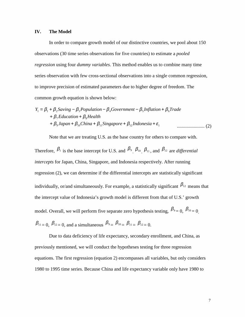
In order to compare growth model of our distinctive countries, we pool about 150

observations (30 time series observations for five countries) to estimate a pooled

regression using four dummy variables. This method enables us to combine many time

series observation with few cross-sectional observations into a single common regression,

to improve precision of estimated parameters due to higher degree of freedom. The

common growth equation is shown below:

TradeInflationGovernmentPopulationSavingY 6543211 ββββββ +−−−+= HealthEducation 87 ββ ++

11211109 εββββ +++++ IndonesiaSingaporeChinaJapan ....................... (2)

Note that we are treating U.S. as the base country for others to compare with.

Therefore, 1β is the base intercept for U.S. and 9β, 10β

, 11β , and 12β are differential

intercepts for Japan, China, Singapore, and Indonesia respectively. After running

regression (2), we can determine if the differential intercepts are statistically significant

individually, or/and simultaneously. For example, a statistically significant 12β means that

the intercept value of Indonesia’s growth model is different from that of U.S.’ growth

model. Overall, we will perform five separate zero hypothesis testing, 9β = 0, 10β = 0,

11β = 0, 12β = 0, and a simultaneous 9β = 10β = 11β = 12β = 0.

Due to data deficiency of life expectancy, secondary enrollment, and China, as

previously mentioned, we will conduct the hypotheses testing for three regression

equations. The first regression (equation 2) encompasses all variables, but only considers

1980 to 1995 time series. Because China and life expectancy variable only have 1980 to

8

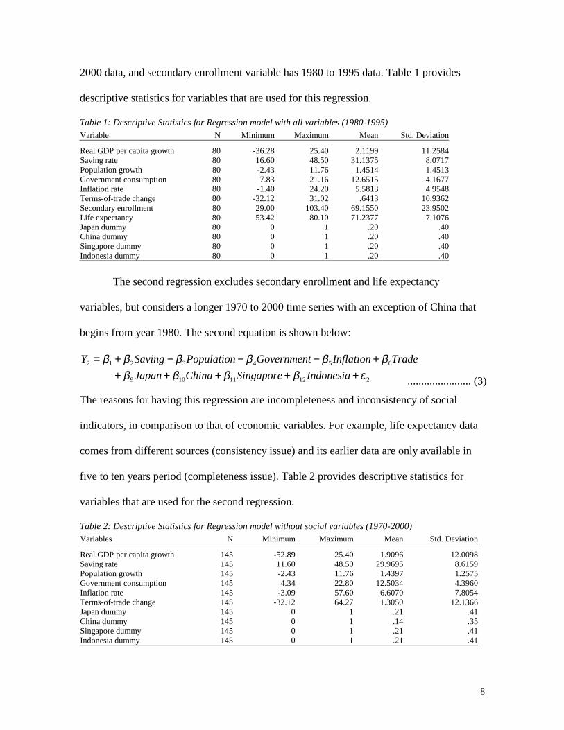
2000 data, and secondary enrollment variable has 1980 to 1995 data. Table 1 provides

descriptive statistics for variables that are used for this regression.

Table 1: Descriptive Statistics for Regression model with all variables (1980-1995) Variable N Minimum Maximum Mean Std. Deviation

Real GDP per capita growth 80 -36.28 25.40 2.1199 11.2584 Saving rate 80 16.60 48.50 31.1375 8.0717 Population growth 80 -2.43 11.76 1.4514 1.4513 Government consumption 80 7.83 21.16 12.6515 4.1677 Inflation rate 80 -1.40 24.20 5.5813 4.9548 Terms-of-trade change 80 -32.12 31.02 .6413 10.9362 Secondary enrollment 80 29.00 103.40 69.1550 23.9502 Life expectancy 80 53.42 80.10 71.2377 7.1076 Japan dummy 80 0 1 .20 .40 China dummy 80 0 1 .20 .40 Singapore dummy 80 0 1 .20 .40 Indonesia dummy 80 0 1 .20 .40

The second regression excludes secondary enrollment and life expectancy

variables, but considers a longer 1970 to 2000 time series with an exception of China that

begins from year 1980. The second equation is shown below:

TradeInflationGovernmentPopulationSavingY 6543212 ββββββ +−−−+= 21211109 εββββ +++++ IndonesiaSingaporeChinaJapan ....................... (3)

The reasons for having this regression are incompleteness and inconsistency of social

indicators, in comparison to that of economic variables. For example, life expectancy data

comes from different sources (consistency issue) and its earlier data are only available in

five to ten years period (completeness issue). Table 2 provides descriptive statistics for

variables that are used for the second regression.

Table 2: Descriptive Statistics for Regression model without social variables (1970-2000) Variables N Minimum Maximum Mean Std. Deviation

Real GDP per capita growth 145 -52.89 25.40 1.9096 12.0098 Saving rate 145 11.60 48.50 29.9695 8.6159 Population growth 145 -2.43 11.76 1.4397 1.2575 Government consumption 145 4.34 22.80 12.5034 4.3960 Inflation rate 145 -3.09 57.60 6.6070 7.8054 Terms-of-trade change 145 -32.12 64.27 1.3050 12.1366 Japan dummy 145 0 1 .21 .41 China dummy 145 0 1 .14 .35 Singapore dummy 145 0 1 .21 .41 Indonesia dummy 145 0 1 .21 .41

9

The third regression is similar to equation (2), in terms of using 1980 to 1995 time

series, except that we perform additional hypothesis testing ( 0β = 0) to compare growth

effects of terms of trade change between U.S. and China. If the differential slope

coefficient ( 0β ) is significant, it means that their terms of trade change effects on growth

are different. The third equation is shown below:

TradeInflationGovernmentPopulationSavingY 6543213 ββββββ +−−−+= HealthEducation 87 ββ ++

IndonesiaSingaporeChinaJapan 1211109 ββββ ++++ 30 . εβ ++ TradeChina ....................... (4)

This equation also enhances the result of equation (2) because it considers both interrupt

and slope differentials, although not all slope differentials from all possible combination of

country-dummy and social-economic variables. We exclude other slope differentials to

avoid lenghty interpretations later. Therefore this regression is experimental by this nature.

We realize that our pooled regression method implicitly makes key assumptions

regarding regression parameters and the stochastic error term. First, we assume that the

parameters do not change over time (temporal stability) and do not differ between various

cross-sectional countries (cross-sectional stability). We believe that having 15 years (1980-

1995) data in equation (2) and (4), and 30 years (1970-2000) data in equation (3) improve

the temporal stability. We certainly solve part of the cross-sectional stability by having

differential intercepts in our equations, but still allowing most differential slopes to be the

same. In other words, we disregard complete interaction effects or interaction dummy

among countries. Considering that having five countries will multiply the number of

interaction dummy thus complicating our model and interpretation afterward. Second, we

assume that error variances of the five countries’ growth equations are homoscedastic, and

10

the error in country A’s equation at time t is uncorrelated with that of country B at time t.

These are the usual Ordinary Least Square properties that we assume to be true in our case.

If we accept these assumptions and later find that differential intercepts are

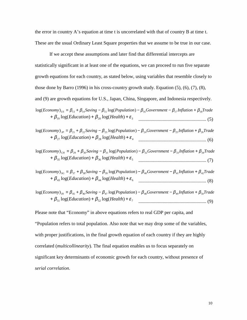
statistically significant in at least one of the equations, we can proceed to run five separate

growth equations for each country, as stated below, using variables that resemble closely to

those done by Barro (1996) in his cross-country growth study. Equation (5), (6), (7), (8),

and (9) are growth equations for U.S., Japan, China, Singapore, and Indonesia respectively.

TradeInflationGovernmentPopulationSavingEconomy US 181716151413 )log()log( ββββββ +−−−+=

32019 )log()log( εββ +++ HealthEducation ........................................................ (5)

TradeInflationGovernmentPopulationSavingEconomy JP 262524232221 )log()log( ββββββ +−−−+=


TradeInflationGovernmentPopulationSavingEconomy CH 343332313029 )log()log( ββββββ +−−−+=


TradeInflationGovernmentPopulationSavingEconomy SG 424140393837 )log()log( ββββββ +−−−+=


TradeInflationGovernmentPopulationSavingEconomy IN 504948474645 )log()log( ββββββ +−−−+=


Please note that “Economy” in above equations refers to real GDP per capita, and

“Population refers to total population. Also note that we may drop some of the variables,

with proper justifications, in the final growth equation of each country if they are highly

correlated (multicollinearity). The final equation enables us to focus separately on

significant key determinants of economic growth for each country, without presence of

serial correlation.

11

For these country regression runs, we use two years period of data since annual

frequency will likely be affected by business-cycle effect. We realize that longer intervals,

such as five or ten years, are probably more effective to smooth out the cyclical effect. But

since we have only 20 years dataset for China, and we need at least 10 cases to assess the

significance of the result, we have to settle on 2-years period.

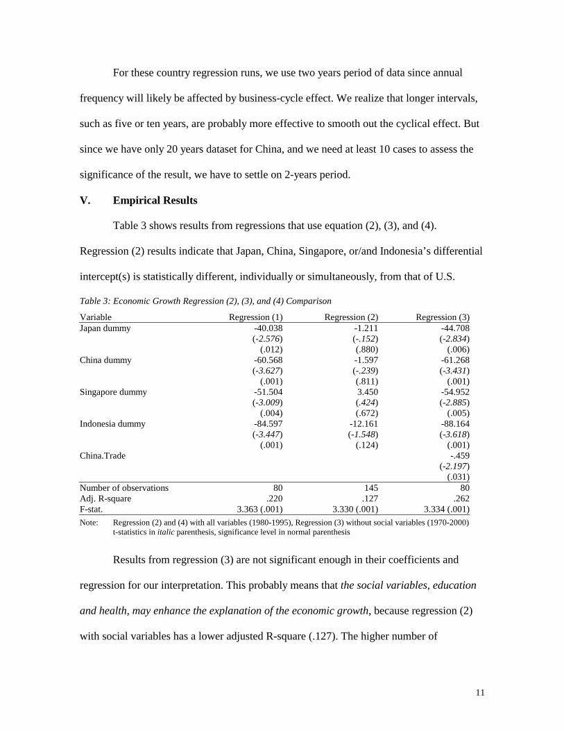
V. Empirical Results

Table 3 shows results from regressions that use equation (2), (3), and (4).

Regression (2) results indicate that Japan, China, Singapore, or/and Indonesia’s differential

intercept(s) is statistically different, individually or simultaneously, from that of U.S.

Table 3: Economic Growth Regression (2), (3), and (4) Comparison

Variable Regression (1) Regression (2) Regression (3) Japan dummy -40.038

(-2.576) (.012)

-1.211 (-.152) (.880)

-44.708 (-2.834)

(.006) China dummy -60.568

(-3.627) (.001)

-1.597 (-.239) (.811)

-61.268 (-3.431)

(.001) Singapore dummy -51.504

(-3.009) (.004)

3.450 (.424) (.672)

-54.952 (-2.885)

(.005) Indonesia dummy -84.597

(-3.447) (.001)

-12.161 (-1.548)

(.124)

-88.164 (-3.618)

(.001) China.Trade -.459

(-2.197) (.031)

Number of observations 80 145 80 Adj. R-square .220 .127 .262 F-stat. 3.363 (.001) 3.330 (.001) 3.334 (.001) Note: Regression (2) and (4) with all variables (1980-1995), Regression (3) without social variables (1970-2000) t-statistics in italic parenthesis, significance level in normal parenthesis

Results from regression (3) are not significant enough in their coefficients and

regression for our interpretation. This probably means that the social variables, education

and health, may enhance the explanation of the economic growth, because regression (2)

with social variables has a lower adjusted R-square (.127). The higher number of

12

observations in regression (3) does not help its significant either. This is probably due to

higher business cycles effect from more frequent observation.

China.Trade coefficient is significant at 3% level, which means that China’s trade

variable is different from that of United States in affecting growth. US’ terms of trade have

not improved since 1991, but it can afford to do so because of its huge domestic economy.

On the other side, China has to depend more on his export to spur growth. This extra

variable in equation (4) slightly improves equation (2) as can bee seen from a higher

adjusted R-square (.262). Based on the results of regression (2) and (4), we can say that

Japan, China, Singapore, and Indonesia seem to have different economic growth models

than that of United States. If this is the case, the next question is what are key determinants

that may explain differences of their growth models.

Table 4: Correlation Matrix among Economic Growth Regressors for United States, Japan, China, Singapore, and Indonesia (only significant high correlations are shown) Population Government Inflation Trade Education Health Saving USA Japan -.876 -.747 .782 -.791 -.866 China .702 .636 .742 Singapore -.650 -.592 Indonesia .651 .710 .690 Population USA -.892 -.600 .889 .974 Japan .607 -.759 .913 .993 China -.796 .907 .865 Singapore -.582 .645 .952 Indonesia -.544 .975 .969 Government USA -.714 -.869 Japan .644 .619 China -.666 -.644 Singapore -.507 Indonesia Inflation USA -.532 -.503 Japan -.660 -.746 China Singapore Indonesia .737 Trade USA Japan China Singapore .704 Indonesia Education USA .923 Japan .939 China .705 Singapore .581 Indonesia .951

13

Before we discuss those determinants, we detect if any of those variables are highly

correlated. For example, Table 4 shows that health and education variables of U.S. are

highly correlated. Therefore we drop one of the variables such that it optimizes the

significant of coefficients and the regression, and the adjusted R-square. For U.S. final

equation, we drop saving, population, government, inflation, and health. It does not mean

that these variables are not determinants of U.S. growth. It merely says that education and

trade seem to play a more significant role in its growth during 1970-2000. The same logic

applies to other countries as well. The Durbin-Watson statistics suggest no strong evidence

of serial correlation. Therefore we are comfortable to present the remaining variables as

significant key determinants of growth for respective countries as shown in Table 5.

Table 5: Economic Growth Regression Results of United States, Japan, China, Singapore, and Indonesia

Log(real GDP per capita) United States Japan China Singapore Indonesia

Saving rate .111 (6.392)

(.000)

1.611E-02 (2.205)

(.046)

Log(population growth)

Government consumption ratio

.241 (4.162)

(.001) Inflation rate -4.877E-02

(-3.821) (.002)

-2.945E-02 (-3.728)

(.007)

Terms-of-trade change -7.850E-03 (-2.342)

(.036)

9.734E-03 (2.324)

(.053)

Log(secondary enrollment ratio)

1.590 (4.953)

(.000)

7.408 (6.528)

(.000)

Log(life expectancy) 9.792 (19.541)

(.000)

-2.635 (-4.778)

(.000) Adj. R-square

.681 .913 .795 .968

.811

Durbin-Watson

1.505 1.131 1.666 2.183 1.579

Number of observations

16 16 11 16 16

F-stat 17.040 (.000)

79.952 (.000)

13.899 (.002)

226.754 (.000)

33.130 (.000)

Note: t-statistics in italic parenthesis, significance level in normal parenthesis

14

1. Saving Rate

In the neoclassical model for a closed economy, the saving rate is equal to the ratio

of investment to output. This should justify our use of gross capital formation ratio to GDP

as a proxy to saving rate. We learn from the previous discussion of neoclassical that saving

rate may not affect long-run growth rate without exogenous technological factor.

Empirically, Blomstrom, Lipsey, Zejan (1993) and Barro (1996) reach the following

conclusion regarding investment and growth. They find that their relations are reverse

causation, meaning that an investment decision in a particular economy relate to its growth

opportunity. Barro (1996) concludes this after finding that the estimated coefficient of the

investment variable is statistically significant only if he use a more recent, compared to the

previous five years, investment ratio. Table 5 shows that saving rates are significant

growth factors for China and Singapore. For a one percent increase in saving rate, the real

GDP per capita grows on average at 11.1 percent for China, and 1.6 percent for

Singapore. Because China has a lower current level of per capita output than that of

Singapore, capital accumulation in China has a higher marginal product. Whereas

Singapore probably experiences diminishing marginal product of capital, as predicted by

neoclassical theory.

2. Population Growth

As population grow, more capitals are required for additional labor, instead of

increasing capital per labor. This is why we should expect that a higher population growth

rate has a negative effect on economic output per capita based on neoclassical theory. We

use log of population growth rate rather than log of fertility rate in Barro (1996) because of

data adequacy issue. Barro attributes a significant negative coefficient of the fertility rate to

15

the increased resources that must be devoted to child rearing, rather than to production of

goods (see Becker and Barro, 1988). None of our countries have population growth rates

as significant growth factors, because they are highly (and positively) correlated to

education and health factors (see Table 4). This means that as population grows,

secondary enrollment ratio and life expectancy increases as well, assuming that total

spending in education and health grow at the same time.

3. Government Consumption

Our use of government consumption ratio to GDP to measure government spending

is intended to approximate the size of government in relative to economy. Big government

means higher non-productive (government) spending, and its associated taxation, because

it “crowds out” higher return (more productive) private spending. Therefore we should

expect a negative effect of higher government consumption ratio on economic growth.

Please note that Barro (1996) excludes education and defense spending in his government

consumption variable. His estimated coefficient is negatively significant. Contrarily, we

have a positive significant coefficient for Indonesia. Specifically, for a one percent

increase in government consumption ratio, real GDP per capita of Indonesia increases on

average by 24%. This probably means that private sector is not functioning well because of

ineffectiveness rule of law and political instability. Inclusion of these factors should

capture these effects separately.

4. Inflation Rate

The general view is that inflation is costly, whether it is the average rate of inflation

or the variability and uncertainty of inflation. The reason is that businesses rely on stable

and predictable inflation to perform properly. But how bad is inflation before it reduces

16

growth? Barro (1996) estimates that an increase in the average inflation rate by 10

percentage points per year will lower the growth rate of real per capita GDP by 0.3-0.4

percentage points per year. This means that the level of real GDP will be lowered after 30

years by 6-9%. Therefore the magnitude of the effect is not that large and takes a longer

term. We have a bigger magnitude effect than the one reported by Barro. Table 5 shows

that for a one percent increase in inflation rate, real GDP per capita decreases on average

by 2.9 percent for China and 4.9 percent for Japan. This bigger magnitude probably

reflects business cycles effects due to shorter interval frequency of our observations.

5. Terms of Trade

Changes in terms of trade – measured as the ratio of export to import – has often

been thought as important effect on developing countries, which has to rely on their

exports in key products. But the improvement in this ratio does not always mean a positive

impact on real GDP. We can see in the case of oil importing country that cuts production

and employment due to increase in oil prices. Barro (1996) shows that change in terms of

trade has a significant positive coefficient. But our results are mixed. This trade variable

has a small positive impact (0.79%) on growth for China, but a small negative impact (-

0.97%) for U.S. We interpret this as China is more dependent on trade for growth than U.S.

6. Secondary Enrollment

This education variable is an important part of human capital, especially in

industrialized countries. In fact, Mankiw, Romer, and Weil (1992) report that the share of

human capital factor is about one third of production function in those countries. Although

this factor is a more difficult element to measure precisely, Barro (1996) manages to use

average years of schooling at the secondary and higher level for males aged 25 and over as

17

a proxy for human capital. Since this data is only available at 5 years period, we have to

use gross enrollment ratio for secondary level regardless of age and sex. This is a better

explanatory variable than a lower level, e.g. primary, education according to Barro. His

result shows a significantly positive effect on growth from the years of schooling that

apply across 100 countries. Specifically, an extra year of male upper-level schooling is

estimated to raise growth rate by a substantial 1.2 percentage points per year. Our results

show that both U.S. and Japan have education variable as key determinants of growth.

Specifically, for a one percent increase in secondary enrollment ratio, real GDP per

capita increases on average by 1.6 percent for U.S., and 7.4% for Japan. As developed

countries, U.S. and Japan have to rely more on human capital and less on physical capital

and raw labor to spur growth.

7. Life Expectancy

Dornbusch, Fischer, and Startz (1998) mention that health factor is probably a

major contributor to human capital in poor countries. We should be able to support this

view from our findings in Table 5. But first the cross-country result by Barro (1996) shows

that the log of life expectancy at birth5 has a significantly positive effect on growth. He

interprets this result by broadly proxying life expectancy to the quality of human capital.

Our results are mixed in this case. Human clearly has a strong positive impact on growth

for Singapore, but a negative impact for Indonesia. For a one percent increase in life

expectancy at birth, real GDP per capita increases by 9.8 percent for Singapore, but

decreases by 2.6 percent for Indonesia. Major improvement in health status of Singapore

has coincided with their substantial increments of economic growth. But a health upgrade

5 Barro reports a similar result for infant mortality rate, instead of life expectancy, as a proxy for health.

18

in Indonesia, without a proportionate upgrade in education, seems to create a social burden

that suppresses its growth.

In addition to these seven variables, we would like readers to consider these

differences as well to explain distinctive growth between U.S. and the other four countries:

initial GDP level, rule-of-law effectiveness, political freedom, and religion. Country with a

lower initial GDP level tends to grow at a higher rate, assuming other explanatory

variables are held constant (Barro and Sala-i-Martin, 1995). One of these omitted

explanatory variables that worths mentioning is infrastructure investment. Country without

proper infrastructure in place (i.e. Afghanistan) will have stalled growth rate irrespective of

its initial GDP level. Discussions of law, political, and religion factors are beyond the

scope of this paper. Instead, we will focus on the findings of our seven variables.

Different key determinants of growth for U.S., Japan, China, Singapore, and

Indonesia provide some explanation of why growth models of the last four countries are

different from that of U.S. This result should alert policy makers that no common growth

policy could be fitted to a particular country. Differences in the seven explanatory

variables have to be considered as well. Particularly for U.S. and Japan, education should

be on the top of their agendas. For China, Singapore, and Indonesia, policy makers should

give priorities to saving, health, and law-political correspondingly.

VI. Conclusion

Empirical findings from 1980 to 1995 suggest that economies of China, Japan,

Singapore, and Indonesia grow differently than that of United States. The social indicators,

education and health, explain some of these differences. One small experiment shows that

19

the trade effect on growth is different between China and U.S. But looking at each

economy separately, we find that each has different key determinants of growth.

Higher secondary level enrollment and terms of trade deterioration enhances

growth of U.S. Whereas Japan has higher secondary level enrollment and lower inflation

rate as key growth factors. Growth of China is stimulated by higher saving rate, lower

inflation rate, and terms of trade improvement. Higher life expectancy and saving rate

mostly explain growth of Singapore. But lower life expectancy and higher government

spending ratio correlates to increased growth of Indonesia. Overall, increased secondary

level enrollment is a key growth determinant of U.S. and Japan. Higher saving rate is an

important growth factor of China. Improved life expectancy highly coincides with the

growth of Singapore. Higher government consumption ratio and lower life expectancy

equally explains the growth of Indonesia.

The challenge of time series growth regression for few countries is to overcome

business cycle effect by having higher interval frequencies observations. But some

developing countries, such as China, have only about 20 years of data. Future research will

enable a more accurate analysis using five or ten years of more observations. Other

possible growth research can be taken by incorporating additional social and political

institution factors, such as rule of law (see Barro, 1996), democracy (see Barro, 1999), and

religion (see Iannaccone, 1998).

20

References

Barro, Robert J. “Economic Growth in a Cross Section of Countries.” The Quarterly

Journal of Economics, Vol. 106, Issue 2 (May, 1991), 407-443.

Barro, Robert J. “Determinants of Economic Growth: A Cross-Country Empirical Study.”

NBER Working Paper 5698, August 1996.

Barro, Robert J. “Determinants of Democracy.” The Journal of Political Economy, Vol.

107, Issue 6, Part 2 (Dec., 1999), S158-S183.

Barro, Robert J. and Xavier Sala-i-Martin. “Convergence.” The Journal of Political

Economy, Vol. 100, Issue 2 (Apr., 1992), 223-251.

Becker, Gary S. and Robert J. Barro. “A Reformulation of the Economic Theory of

Fertility.” Quarterly Journal of Economics, 103, 1 (February, 1988), 1-25.

Blomstrom, Magnus, Robert E. Lipsey, and Mario Zejan. “Is Fixed Investment the Key to

Economic Growth?” National Bureau of Economic Research, working paper no. 4436,

August, 1993.

Cass, David. “Optimum Growth in a Aggregative Model of Capital Accumulation.”

Review of Economic Studies, 32, July, 1965, 233-240.

Dornbusch, Rudiger, Stanley Fischer, and Richard Startz. Macroeconomics, 7th ed. New

York: McGraw-Hill, 1998.

Iannaccone, Laurence R. “Introduction to the Economics of Religion.” Journal of

Economic Literature, Vol. 36, Issue 3 (Sep., 1998), 1465-1495.

Koopmans, Tjalling C. “On the Concept of Optimal Economic Growth.” in The

Econometric Approach to Development Planning, Amsterdam, North Holland, 1965.

21

Lucas, Robert E. “On the Mechanics of Economic Development.” Journal of Monetary

Economics, July 1988.

Mankiw, N. G., D. Romer, and D. Weil. “A Contribution to the Empirics of Economic

Growth.” Quarterly Journal of Economics, May 1992.

Romer, Paul. “ Increasing Returns and Long-Run Growth.” Journal of Political Economy,

October 1986.

Sachs, Jeffrey D. “The Wrong Medicine for Asia.” New York Times, November 3, 1997.

Sanger, David E. “I.M.F. Reports Plan Backfired, Worsening Indonesia Woes.” New York

Times, January 14, 1998.

Solow, Robert M. “A Contribution to the Theory of Economic Growth.” Quarterly Journal

of Economics, 70, February, 1956, 65-94.

Swan, Trevor W. “Economic Growth and Capital Accumulation.” Economic Record, 32,

November, 1956, 334-361.

22

Appendix A: Variables Description and Sources

Economy: Annual growth rate of real GDP per capita. Current GDP in local

currency are deflated at 1995 constant price, and then converted to IMF’s SDR currency6,

before divided by total population. Source: International Financial Statistics Year Book,

1999-2001, IMF.

Saving: Gross capital formation as a percentage of GDP. Sources: International

Financial Statistics Year Book, 1999-2001, IMF, and The World Bank Group, World

Development Indicators database.

Population: Annual population growth rate. Sources: International Financial

Statistics Year Book, 1999-2001, IMF, and The World Bank Group, World Development

Indicators database.

Government: Government consumption as a percentage of GDP. Sources:

International Financial Statistics Year Book, 1999-2001, IMF, and Asian Development

Bank (ADB).

Inflation: Annual change of consumer price index. Sources: International Financial

Statistics Year Book, 1999-2001, IMF; The World Bank Group, World Development

Indicators database; and San Jose State University, Economics Dept., Dr. Watkins (China,

1979-1986).

Trade: Annual change of terms of trade, that is export (fob) to import (cif) ratio.

The trade data are based on custom data. Source: International Financial Statistics Year

Book, 1999-2001, IMF.

6 SDR or Special Drawing Rights is determined using a basket of currencies (US$, Euro, Yen, Pound). Weights are assigned to the currencies to reflect their relative importance in world’s trading and financial systems.

23

Education: Gross secondary enrollment ratio, that is total enrollment in secondary

level, regardless of age, expressed as a percentage of the official school-age population

corresponding to secondary level. Sources: UNESCO online database.

Health: life expectancy at birth in years. Source: U.S. Bureau of the Census,

International Data Base; National Center for Health Statistics, National Vital Statistics

Report, Vol. 47, No. 28, Dec 13, 1999; Berkeley Mortality Database (Ministry of Health

and Welfare, Statistics and Information Department); and The World Bank Group, World

Development Indicators database.

Japan: A Dummy variable that takes a value of 1 if the data belong to Japan, or 0

otherwise.

China: A dummy variable that takes a value of 1 if the data belong to Mainland

China only, excludes Hong Kong and Macao, or 0 otherwise.

Singapore: A Dummy variable that takes a value of 1 if the data belong to

Singapore, or 0 otherwise.

Indonesia: A Dummy variable that takes a value of 1 if the data belong to

Indonesia, or 0 otherwise.

Note: If all dummy variables take zero value, the data belong to United States.

24

Appendix B: Data available for regressions

Year Economy Saving Population Government Inflation Trade Education Health Japan China Singapore Indonesia

Growth rate % rate % Growth % % of GDP rate % Change % Enrollment

ratio % Years Dummy Dummy Dummy Dummy 1970 -4.91 17.40 1.17 22.80 5.90 3.79 83.70 70.80 0 0 0 0 1971 -6.04 18.50 1.27 22.24 4.30 -10.48 71.10 0 0 0 0 1972 4.37 19.50 1.08 21.78 3.30 -7.22 71.20 0 0 0 0 1973 -5.95 20.30 0.96 20.78 6.20 15.76 71.40 0 0 0 0 1974 -2.73 19.50 0.92 21.48 11.00 -7.31 72.00 0 0 0 0 1975 3.14 17.00 0.99 22.08 9.10 14.64 84.40 72.60 0 0 0 0 1976 5.39 18.70 0.96 21.08 5.70 -14.26 72.90 0 0 0 0 1977 -0.97 20.20 1.01 20.44 6.50 -12.88 73.30 0 0 0 0 1978 -2.73 21.40 1.07 19.84 7.60 2.09 73.50 0 0 0 0 1979 0.93 21.60 1.11 19.62 11.30 6.97 73.90 0 0 0 0 1980 1.99 19.70 1.20 20.38 13.50 4.67 91.20 73.70 0 0 0 0 1981 11.05 20.60 0.96 20.16 10.30 -0.51 94.40 74.10 0 0 0 0 1982 2.49 18.20 0.97 21.00 6.20 -2.76 94.60 74.50 0 0 0 0 1983 8.88 18.20 0.92 20.82 3.20 -10.27 96.90 74.60 0 0 0 0 1984 13.59 20.80 0.88 20.36 4.30 -15.13 96.10 74.70 0 0 0 0 1985 -8.15 19.70 0.90 20.85 3.60 -3.99 97.30 74.70 0 0 0 0 1986 -8.03 19.20 0.92 21.16 1.90 -4.29 97.70 74.70 0 0 0 0 1987 -11.64 19.90 0.90 21.04 3.70 0.76 96.65 74.90 0 0 0 0 1988 8.81 19.00 0.91 20.30 4.00 17.19 94.55 74.90 0 0 0 0 1989 5.04 19.10 0.93 20.04 4.80 5.19 93.50 75.10 0 0 0 0 1990 -6.98 18.00 1.06 20.36 5.40 3.15 93.10 75.40 0 0 0 0 1991 -2.05 16.60 1.08 20.64 4.20 8.97 94.50 75.50 0 0 0 0 1992 6.08 16.90 1.08 20.11 3.00 -2.47 97.30 75.80 0 0 0 0 1993 1.62 17.40 1.06 19.47 3.00 -4.80 98.50 75.75 0 0 0 0 1994 -3.06 18.50 0.98 18.82 2.60 -3.43 97.30 75.70 0 0 0 0 1995 -0.07 18.30 0.94 18.54 2.80 1.99 97.40 75.79 0 0 0 0 1996 6.13 18.70 0.92 18.20 2.90 0.24 76.12 0 0 0 0 1997 9.99 19.40 0.96 17.84 2.30 0.74 76.51 0 0 0 0 1998 -0.97 20.20 0.95 17.46 1.60 -5.71 76.70 0 0 0 0 1999 5.87 20.30 0.95 17.61 2.20 -8.25 76.98 0 0 0 0 2000 7.62 21.40 3.04 17.50 3.40 -6.28 77.12 0 0 0 0 1970 8.02 39.00 1.13 7.44 7.70 -3.88 86.60 72.00 1 0 0 0 1971 7.72 35.80 1.30 7.96 6.40 18.98 72.94 1 0 0 0 1972 11.32 35.50 1.41 8.16 4.90 0.14 73.54 1 0 0 0 1973 3.40 38.10 1.42 8.30 11.70 -20.89 73.79 1 0 0 0 1974 -10.69 37.30 1.33 9.12 23.10 -7.14 74.41 1 0 0 0 1975 4.41 32.80 1.28 10.04 11.80 7.74 91.80 75.08 1 0 0 0 1976 8.99 31.80 1.08 9.86 9.40 7.51 75.48 1 0 0 0 1977 21.68 30.80 0.97 9.83 8.20 9.59 75.93 1 0 0 0 1978 19.72 30.90 0.91 9.66 4.10 8.12 76.09 1 0 0 0 1979 -16.30 32.50 0.84 9.70 3.80 -24.20 76.42 1 0 0 0 1980 25.40 32.20 0.81 9.81 7.80 -0.89 93.20 76.20 1 0 0 0 1981 4.09 31.10 0.73 9.92 4.90 14.86 93.50 76.54 1 0 0 0 1982 1.14 29.90 0.70 9.90 2.70 -0.76 93.10 77.06 1 0 0 0 1983 8.71 28.10 0.70 9.94 1.90 10.45 92.40 77.10 1 0 0 0 1984 2.28 28.00 0.65 9.80 2.20 7.21 93.10 77.51 1 0 0 0 1985 16.67 28.20 0.63 9.58 2.00 8.95 95.40 77.80 1 0 0 0 1986 15.50 27.70 0.54 9.65 0.60 21.70 96.20 78.23 1 0 0 0 1987 15.12 28.50 0.49 9.43 0.10 -7.32 96.60 78.65 1 0 0 0 1988 9.44 30.40 0.40 9.14 0.70 -7.70 96.80 78.40 1 0 0 0 1989 -6.35 31.30 0.40 9.07 2.30 -7.59 96.40 78.84 1 0 0 0 1990 2.99 32.30 0.33 9.02 3.10 -6.46 97.10 79.07 1 0 0 0 1991 10.34 32.20 0.39 9.02 3.30 8.71 96.40 79.39 1 0 0 0 1992 5.10 30.80 0.37 9.18 1.70 9.71 95.70 79.47 1 0 0 0 1993 11.63 29.70 0.33 9.42 1.30 2.88 98.90 79.63 1 0 0 0 1994 5.97 28.70 0.28 9.54 0.70 -3.79 99.60 80.10 1 0 0 0 1995 -3.60 28.60 0.23 9.81 -0.10 -8.54 103.40 79.96 1 0 0 0 1996 -3.99 30.00 0.23 9.68 0.10 -10.79 80.21 1 0 0 0 1997 -3.72 28.60 0.25 9.72 1.70 5.59 80.33 1 0 0 0 1998 4.35 26.30 0.27 10.17 0.60 11.30 80.45 1 0 0 0

25



ratio % Years Dummy Dummy Dummy Dummy 1999 12.07 26.11 0.08 10.29 -0.30 -2.58 80.57 1 0 0 0 2000 -2.89 25.90 0.28 16.60 -0.60 -6.27 80.70 1 0 0 0 1970 2.88 -20.11 24.30 61.70 0 1 0 0 1971 2.70 29.13 0 1 0 0 1972 2.29 -0.91 0 1 0 0 1973 2.33 -12.90 63.29 0 1 0 0 1974 1.85 -19.14 63.29 0 1 0 0 1975 1.72 6.33 46.20 63.29 0 1 0 0 1976 1.41 7.46 0 1 0 0 1977 1.33 0.92 0 1 0 0 1978 1.36 13.24 -14.99 67.30 0 1 0 0 1979 36.20 1.33 15.07 2.00 -2.55 0 1 0 0 1980 6.48 34.90 2.12 14.48 6.00 4.14 45.90 67.00 0 1 0 0 1981 -0.79 32.30 1.23 14.38 2.40 10.14 39.40 67.80 0 1 0 0 1982 2.42 32.10 1.21 14.03 1.90 15.78 36.20 68.15 0 1 0 0 1983 10.82 33.00 1.86 13.79 1.50 -10.22 35.70 68.50 0 1 0 0 1984 -14.47 34.50 1.47 14.24 2.80 -8.22 37.40 68.85 0 1 0 0 1985 -10.85 38.50 1.45 13.47 8.80 -32.12 39.70 69.20 0 1 0 0 1986 -17.05 38.00 1.54 13.49 6.00 11.41 42.50 69.33 0 1 0 0 1987 -5.48 36.70 1.61 12.64 7.20 26.53 44.80 69.46 0 1 0 0 1988 15.41 37.40 1.60 11.75 18.70 -5.79 45.60 68.98 0 1 0 0 1989 -17.21 37.00 1.54 12.35 18.30 3.33 46.10 68.50 0 1 0 0 1990 -14.50 35.20 1.41 12.29 3.10 31.02 48.70 68.37 0 1 0 0 1991 3.08 35.30 1.28 13.30 3.50 -3.15 51.80 68.67 0 1 0 0 1992 10.92 37.30 1.15 13.50 6.30 -6.50 55.00 68.97 0 1 0 0 1993 11.55 43.50 1.08 13.04 14.60 -16.28 56.80 69.27 0 1 0 0 1994 -27.98 41.30 1.04 12.82 24.20 18.58 61.00 69.58 0 1 0 0 1995 9.17 40.80 0.97 11.44 16.90 10.14 65.80 69.90 0 1 0 0 1996 12.40 39.30 0.98 11.49 8.30 -5.58 68.90 70.19 0 1 0 0 1997 15.11 38.00 0.95 11.65 2.80 18.19 70.10 70.48 0 1 0 0 1998 2.39 38.10 0.92 11.88 -0.80 1.74 70.78 0 1 0 0 1999 8.89 38.30 0.88 12.95 -1.40 -10.04 71.08 0 1 0 0 2000 14.32 37.93 -0.45 13.09 0.30 2.72 71.38 0 1 0 0 1970 9.85 38.70 1.47 11.94 0.50 -16.88 46.00 65.80 0 0 1 0 1971 7.96 40.20 1.93 12.62 1.80 -1.73 0 0 1 0 1972 14.50 41.10 1.90 12.14 2.10 3.91 0 0 1 0 1973 11.75 39.20 1.86 10.96 19.60 10.50 0 0 1 0 1974 10.58 44.60 1.83 10.35 22.40 -2.69 0 0 1 0 1975 -0.17 37.60 1.35 10.64 2.50 -4.66 51.90 67.55 0 0 1 0 1976 8.38 40.80 1.33 10.52 -1.80 9.82 0 0 1 0 1977 6.26 36.20 1.75 10.70 3.20 8.42 0 0 1 0 1978 8.47 39.00 0.86 11.02 4.90 -1.41 0 0 1 0 1979 7.03 43.40 1.28 9.91 4.10 3.97 0 0 1 0 1980 15.35 46.30 1.26 9.75 8.50 0.04 59.90 71.63 0 0 1 0 1981 21.35 46.30 1.24 9.51 8.20 -5.78 52.60 71.80 0 0 1 0 1982 8.20 47.90 1.23 10.93 3.90 -2.95 54.10 72.22 0 0 1 0 1983 15.71 47.90 -2.43 10.88 1.20 5.06 56.80 72.29 0 0 1 0 1984 11.58 48.50 1.24 10.82 2.60 8.29 59.00 72.85 0 0 1 0 1985 -10.64 42.50 1.64 14.26 0.50 3.36 62.00 73.52 0 0 1 0 1986 -12.43 37.50 1.61 13.42 -1.40 1.60 67.20 74.18 0 0 1 0 1987 -0.40 37.90 1.19 12.37 0.50 -0.08 68.90 74.35 0 0 1 0 1988 8.11 34.20 11.76 10.52 1.50 1.71 69.90 74.46 0 0 1 0 1989 12.18 35.00 2.81 10.33 2.30 0.37 69.90 74.57 0 0 1 0 1990 6.05 36.60 3.07 10.20 3.50 -3.53 68.10 76.04 0 0 1 0 1991 11.48 34.80 2.32 9.94 3.40 2.82 67.40 76.88 0 0 1 0 1992 6.70 36.40 2.91 9.33 2.30 -1.42 67.40 77.09 0 0 1 0 1993 12.62 37.90 2.52 9.37 2.30 -1.27 67.30 77.62 0 0 1 0 1994 11.96 33.50 3.07 8.44 3.10 8.61 72.00 77.86 0 0 1 0 1995 5.99 34.60 3.27 8.57 1.70 0.72 73.40 77.96 0 0 1 0 1996 7.93 37.10 4.03 9.48 1.40 0.21 74.10 78.67 0 0 1 0 1997 -6.86 38.90 3.60 9.54 2.00 -0.85 79.66 0 0 1 0 1998 -6.09 34.20 3.48 10.16 -0.30 11.20 79.79 0 0 1 0 1999 7.12 32.44 0.52 9.70 -3.09 -1.60 79.92 0 0 1 0

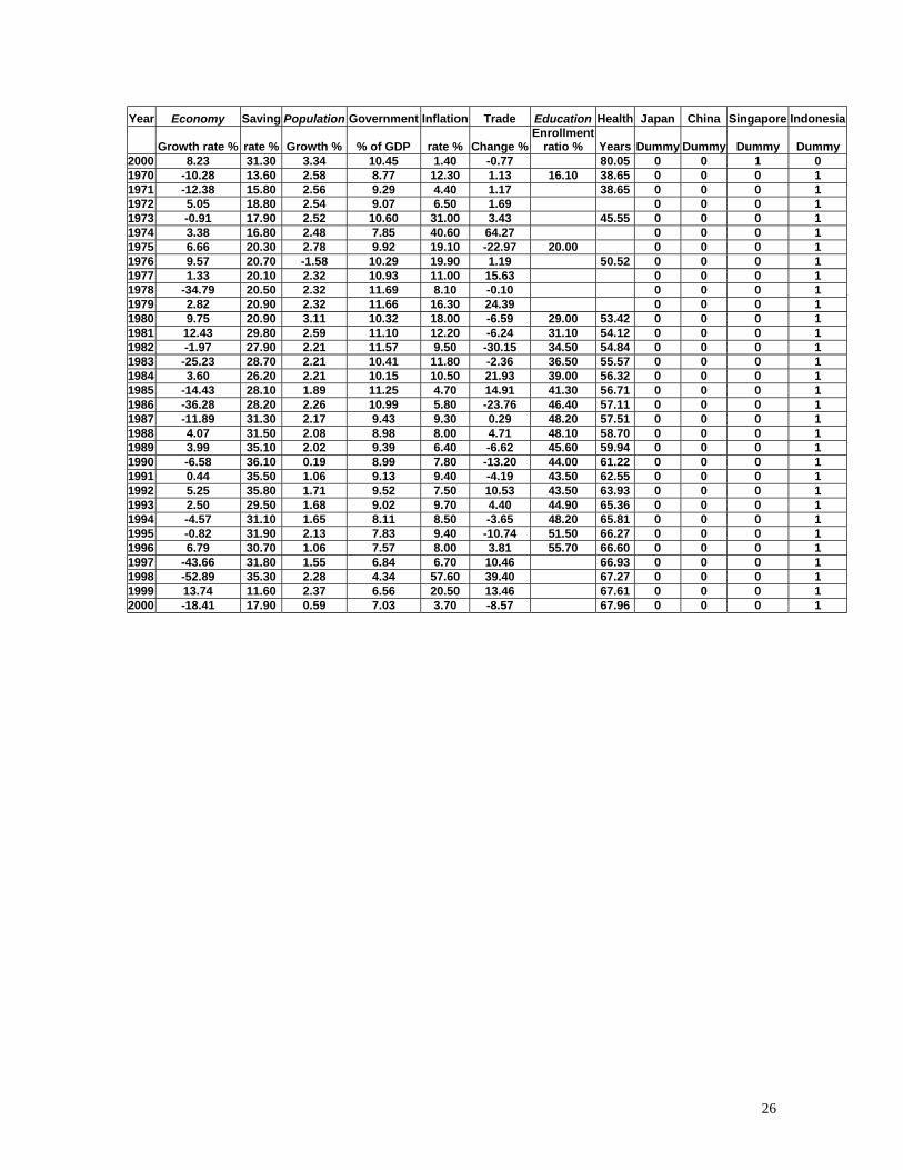
26



ratio % Years Dummy Dummy Dummy Dummy 2000 8.23 31.30 3.34 10.45 1.40 -0.77 80.05 0 0 1 0 1970 -10.28 13.60 2.58 8.77 12.30 1.13 16.10 38.65 0 0 0 1 1971 -12.38 15.80 2.56 9.29 4.40 1.17 38.65 0 0 0 1 1972 5.05 18.80 2.54 9.07 6.50 1.69 0 0 0 1 1973 -0.91 17.90 2.52 10.60 31.00 3.43 45.55 0 0 0 1 1974 3.38 16.80 2.48 7.85 40.60 64.27 0 0 0 1 1975 6.66 20.30 2.78 9.92 19.10 -22.97 20.00 0 0 0 1 1976 9.57 20.70 -1.58 10.29 19.90 1.19 50.52 0 0 0 1 1977 1.33 20.10 2.32 10.93 11.00 15.63 0 0 0 1 1978 -34.79 20.50 2.32 11.69 8.10 -0.10 0 0 0 1 1979 2.82 20.90 2.32 11.66 16.30 24.39 0 0 0 1 1980 9.75 20.90 3.11 10.32 18.00 -6.59 29.00 53.42 0 0 0 1 1981 12.43 29.80 2.59 11.10 12.20 -6.24 31.10 54.12 0 0 0 1 1982 -1.97 27.90 2.21 11.57 9.50 -30.15 34.50 54.84 0 0 0 1 1983 -25.23 28.70 2.21 10.41 11.80 -2.36 36.50 55.57 0 0 0 1 1984 3.60 26.20 2.21 10.15 10.50 21.93 39.00 56.32 0 0 0 1 1985 -14.43 28.10 1.89 11.25 4.70 14.91 41.30 56.71 0 0 0 1 1986 -36.28 28.20 2.26 10.99 5.80 -23.76 46.40 57.11 0 0 0 1 1987 -11.89 31.30 2.17 9.43 9.30 0.29 48.20 57.51 0 0 0 1 1988 4.07 31.50 2.08 8.98 8.00 4.71 48.10 58.70 0 0 0 1 1989 3.99 35.10 2.02 9.39 6.40 -6.62 45.60 59.94 0 0 0 1 1990 -6.58 36.10 0.19 8.99 7.80 -13.20 44.00 61.22 0 0 0 1 1991 0.44 35.50 1.06 9.13 9.40 -4.19 43.50 62.55 0 0 0 1 1992 5.25 35.80 1.71 9.52 7.50 10.53 43.50 63.93 0 0 0 1 1993 2.50 29.50 1.68 9.02 9.70 4.40 44.90 65.36 0 0 0 1 1994 -4.57 31.10 1.65 8.11 8.50 -3.65 48.20 65.81 0 0 0 1 1995 -0.82 31.90 2.13 7.83 9.40 -10.74 51.50 66.27 0 0 0 1 1996 6.79 30.70 1.06 7.57 8.00 3.81 55.70 66.60 0 0 0 1 1997 -43.66 31.80 1.55 6.84 6.70 10.46 66.93 0 0 0 1 1998 -52.89 35.30 2.28 4.34 57.60 39.40 67.27 0 0 0 1 1999 13.74 11.60 2.37 6.56 20.50 13.46 67.61 0 0 0 1 2000 -18.41 17.90 0.59 7.03 3.70 -8.57 67.96 0 0 0 1

determinants of economic growth: u.s., japan, china ... · 1 determinants of economic growth: u.s.,...

Documents