composing schema mappings: second-order dependencies to ... · composing schema mappings:...

Composing Schema Mappings:Second-Order Dependencies to the Rescue

RONALD FAGIN

IBM Almaden Research Center

PHOKION G. KOLAITIS1


LUCIAN POPA


WANG-CHIEW TAN2

University of California, Santa Cruz

A schema mapping is a specification that describes how data structured under one schema (the

source schema) is to be transformed into data structured under a different schema (the targetschema). A fundamental problem is composing schema mappings: given two successive schema

mappings, derive a schema mapping between the source schema of the first and the target schemaof the second that has the same effect as applying successively the two schema mappings.

In this paper, we give a rigorous semantics to the composition of schema mappings and inves-

tigate the definability and computational complexity of the composition of two schema mappings.We first study the important case of schema mappings in which the specification is given by a

finite set of source-to-target tuple-generating dependencies (source-to-target tgds). We show that

the composition of a finite set of full source-to-target tgds with a finite set of tgds is alwaysdefinable by a finite set of source-to-target tgds, but the composition of a finite set of source-to-

target tgds with a finite set of full source-to-target tgds may not be definable by any set (finite

or infinite) of source-to-target tgds; furthermore, it may not be definable by any formula of leastfixed-point logic, and the associated composition query may be NP-complete. After this, we in-

troduce a class of existential second-order formulas with function symbols and equalities, which

we call second-order tgds, and make a case that they are the “right” language for composingschema mappings. Specifically, we show that second-order tgds form the smallest class (up to

logical equivalence) that contains every source-to-target tgd and is closed under conjunction andcomposition. Allowing equalities in second-order tgds turns out to be of the essence, even though

the “obvious” way to define second-order tgds does not require equalities. We show that second-

order tgds without equalities are not sufficiently expressive to define the composition of finite setsof source-to-target tgds. Finally, we show that second-order tgds possess good properties for dataexchange and query answering: the chase procedure can be extended to second-order tgds so that

it produces polynomial-time computable universal solutions in data exchange settings specified bysecond-order tgds.

Categories and Subject Descriptors: H.2.5 [Heterogeneous Databases]: Data translation; H.2.4

1On leave from UC Santa Cruz.2Supported in part by NSF CAREER Award IIS-0347065 and NSF grant IIS-0430994.

A preliminary version of this paper appeared in Proc. 2004 ACM Symposium of Principles ofDatabase Systems, Paris, France, pp. 83–94.

Permission to make digital/hard copy of all or part of this material without fee for personalor classroom use provided that the copies are not made or distributed for profit or commercial

advantage, the ACM copyright/server notice, the title of the publication, and its date appear, andnotice is given that copying is by permission of the ACM, Inc. To copy otherwise, to republish,

to post on servers, or to redistribute to lists requires prior specific permission and/or a fee.c© 20 ACM 0362-5915/20/0300-0001 $5.00

ACM Transactions on Database Systems, Vol. , No. , 20, Pages 1–60.

2 ·

[Systems]: Relational Databases; H.2.4 [Systems]: Query processing

General Terms: Algorithms, Theory

Additional Key Words and Phrases: Data exchange, data integration, composition, schema map-ping, certain answers, conjunctive queries, dependencies, chase, computational complexity, query

answering, second-order logic, universal solution, metadata model management

1. INTRODUCTION & SUMMARY OF RESULTS

The problem of transforming data structured under one schema into data struc-tured under a different schema is an old, but persistent problem, arising in severaldifferent areas of database management systems. In recent years, this problemhas received considerable attention in the context of information integration, wheredata from various heterogeneous sources has to be transformed into data structuredunder a mediated schema. To achieve interoperability, data-sharing architecturesuse schema mappings to describe how data is to be transformed from one represen-tation to another. These schema mappings are typically specified using high-leveldeclarative formalisms that make it possible to describe the correspondence be-tween different schemas at a logical level, without having to specify physical detailsthat may be relevant only for the implementation (run-time) phase. In particular,declarative schema mappings in the form of GAV (global-as-view), LAV (local-as-view), and, more generally, GLAV (global-and-local-as-view) assertions have beenused in data integration systems [Lenzerini 2002]. Similarly, source-to-target tuple-generating dependencies (source-to-target tgds) have been used for specifying dataexchange between a relational source and a relational target [Fagin, Kolaitis, Millerand Popa 2005; Fagin, Kolaitis and Popa 2003]; moreover, nested (XML-style)source-to-target dependencies have been used in the Clio data exchange system[Popa et al. 2002].

The extensive use of schema mappings has motivated the need to develop a frame-work for managing these schema mappings and other related metadata. Bernstein[Bernstein 2003] has introduced such a framework, called model management , inwhich the main abstractions are schemas and mappings between schemas, as well asoperators for manipulating schemas and mappings. One of the most fundamentaloperators in this framework is the composition operator , which combines successiveschema mappings into a single schema mapping. The composition operator can playa useful role each time the target of a schema mapping is also the source of anotherschema mapping. This scenario occurs, for instance, in schema evolution, where aschema may undergo several successive changes. It also occurs in peer-to-peer datamanagement systems, such as the Piazza System [Halevy, Ives, Mork and Tatari-nov 2003], and in extract-transform-load (ETL) processes in which the output ofa transformation may be input to another [Vassiliadis, Simitsis and Skiadopoulos2002]. A model management system should be able to figure out automatically howto compose two or more successive schema mappings into a single schema mappingbetween the first schema and the last schema in a way that captures the interactionof the schema mappings in the entire sequence. The resulting single schema map-ping can then be used during the run-time phase for various purposes, such as queryACM Transactions on Database Systems, Vol. , No. , 20.

· 3

answering and data exchange, potentially with significant performance benefits.

Bernstein’s approach provides a rich conceptual framework for model manage-ment. The next stage in the development of this framework is to provide a rigorousand meaningful semantics of the basic model management operators and to inves-tigate the properties of this semantics. As pointed out by Bernstein [Bernstein2003], while the semantics of the match operator have been worked out to a certainextent, the semantics of other basic operators, including the composition opera-tor, “are less well developed”. The problem of composing schema mappings hasthe following general formulation: given a schema mapping M12 from schema S1

to schema S2, and a schema mapping M23 from schema S2 to schema S3, derivea schema mapping M13 from schema S1 to schema S3 that is “equivalent” to thesuccessive application of M12 and M23. Thus, providing semantics to the composi-tion operator amounts to making precise what “equivalence” means in this context.Madhavan and Halevy [Madhavan and Halevy 2003] were the first to propose a se-mantics of the composition operator. To this effect, they defined the semantics ofthe composition operator relative to a class Q of queries over the schema S3 by stip-ulating that “equivalence” means that, for every query q in Q, the certain answersof q in M13 coincide with the certain answers of q that would be obtained by suc-cessively applying the two schema mappings M12 and M23. They then establisheda number of results for this semantics in the case in which the schema mappingsM12 and M23 are specified by source-to-target tgds (that is, GLAV assertions),and the class Q is the class of all conjunctive queries over S3. The semantics of thecomposition operator proposed by Madhavan and Halevy is a significant first step,but it suffers from certain drawbacks that seem to be caused by the fact that thissemantics is given relative to a class of queries. To begin with, the set of formulasspecifying a composition M13 of M12 and M23 relative to a class Q of queriesneed not be unique up to logical equivalence, even when the class Q of queries isheld fixed. Moreover, this semantics is rather fragile, because as we show, a schemamapping M13 may be a composition of M12 and M23 when Q is the class of con-junctive queries (the class Q that Madhavan and Halevy focused on), but fail tobe a composition of these two schema mappings when Q is the class of conjunctivequeries with inequalities.

In this paper, we first introduce a different semantics for the composition op-erator and then investigate the definability and computational complexity of thecomposition of schema mappings under this new semantics. Unlike the semanticsproposed by Madhavan and Halevy, our semantics does not carry along a class ofqueries as a parameter. Specifically, we focus on the space of instances of schemamappings and define a schema mapping M13 to be a composition of two schemamappings M12 and M23 if the space of instances of M13 is the set-theoretic com-position of the spaces of instances of M12 and M23, where these spaces are viewedas binary relations between source instances and target instances. One advantageof this approach is that the set of formulas defining a composition M13 of M12 andM23 is unique up to logical equivalence; thus, we can refer to such a schema map-ping M13 as the composition of M12 and M23. Moreover, our semantics is robust,since it is defined in terms of the schema mappings alone and without reference toa set of queries. In fact, it is easy to see that the composition (in our sense) of two

ACM Transactions on Database Systems, Vol. , No. , 20.

4 ·

schema mappings is a composition of these two schema mappings in the sense ofMadhavan and Halevy relative to every class of queries.

We explore in depth the properties of the composition of schema mappings spec-ified by a finite set of source-to-target tuple-generating dependencies (source-to-target tgds). A natural question to ask is whether the composition of two suchschema mappings can also be specified by a finite set of source-to-target tgds; ifnot, in what logical formalism can it be actually expressed? On the positive side, weshow that the composition of a finite set of full source-to-target tgds with a finiteset of source-to-target tgds is always definable by a finite set of source-to-targettgds (a source-to-target tgd is full if no existentially quantified variables occur inthe tgd). On the negative side, however, we show that the composition of a finiteset of source-to-target tgds with a finite set of full source-to-target tgds may notbe definable by any set (finite or infinite) of source-to-target tgds. We also showthat the composition of a finite set of source-to-target tgds with a finite set of fullsource-to-target tgds may not even be definable in the finite-variable infinitary logicLω∞ω, which implies that it is not definable in least fixed-point logic LFP; moreover,

the associated composition query can be NP-complete.

To ameliorate these negative results, we introduce a class of existential second-order formulas with function symbols and equalities, called second-order tgds, whichexpress source-to-target constraints and which subsume the class of finite conjunc-tions of (first-order) source-to-target tgds. We make a case that second-order tgdsare the right language both for specifying schema mappings and for composing suchschema mappings. To begin with, we show that the composition of two finite sets ofsource-to-target tgds is always definable by a second-order tgd. Moreover, the com-position of second-order tgds is also definable by a second-order tgd, and we give analgorithm that, given two schema mappings specified by second-order tgds, outputsa second-order tgd that defines the composition. Furthermore, the conjunction ofa finite set of second-order tgds is equivalent to a single second-order tgd. Hence,the composition of a finite number of schema mappings, each defined by a finite setof source-to-target (second-order) tgds, is always definable by a second-order tgd.It should be pointed out that arriving at the right concept of second-order tgds is arather delicate matter. Indeed, at first one may consider the class of second-orderformulas that are obtained from first-order tgds by Skolemizing the existential first-order quantifiers into existentially quantified function symbols. This process givesrise to a class of existential second-order formulas with no equalities. Therefore,the “obvious” way to define second-order tgds is with formulas with no equalities.Interestingly enough, however, we show that second-order tgds without equalitiesare not sufficiently expressive to define the composition of finite sets of (first-order)source-to-target tgds. In fact, our second-order tgds (with equalities) form thesmallest class of formulas (up to logical equivalence) for composing schema map-pings given by finite sets of source-to-target tgds; every second-order tgd definesthe composition of a finite sequence of schema mappings, each defined by a finiteset of source-to-target tgds.

We then show that second-order tgds possess good properties for data exchange.In particular, the chase procedure can be extended to second-order tgds so that itproduces polynomial-time computable “universal solutions” (in the sense of [Fagin,ACM Transactions on Database Systems, Vol. , No. , 20.

· 5

Kolaitis, Miller and Popa 2005]) in data exchange settings specified by second-ordertgds. As a result, in such data exchange settings the certain answers of conjunctivequeries can be computed in polynomial time.

In spite of the richness of second-order tgds, they form a well-behaved fragmentof second-order logic for composing schema mappings. As we noted earlier, if thedata exchange setting is defined by second-order tgds, then the certain answers ofevery conjunctive query can be computed in polynomial time (by doing the chase).By contrast, when the source schema is described in terms of the target schemaby means of arbitrary first-order views, there are conjunctive queries for whichcomputing the certain answers is an undecidable problem [Abiteboul and Duschka1998]. Thus, our second-order tgds form a fragment of second-order logic that insome ways is more well-behaved than first-order logic.

There is a subtle issue about the choice of universe in the semantics of second-order tgds. We take our universe to be a countably infinite set of elements thatincludes the active domain. This is a natural choice for the universe, since second-order tgds have existentially quantified function symbols and for this reason, oneneeds sufficiently many elements in the universe in order to interpret these functionsymbols without making any unnecessary combinatorial assumptions. In fact, weshow that as long as we take the universe to be finite but sufficiently large, thenthe semantics of a second-order tgd remains unchanged from the infinite universesemantics.

We show that determining whether a given instance over the source and targetschema satisfies a second-order tgd is in NP and can be NP-complete. This is incontrast with the first order case, where such “model checking” can be done inpolynomial time.

Finally, we examine Madhavan and Halevy’s notion of composition, which werefer to as “certain-answer adequacy”. Roughly speaking, a formula is certain-answer adequate if it gives the same certain answers as the composition. A formulaσ that defines the composition (in our sense) is always certain-answer adequate forevery class Q of queries; however, other formulas that are not logically equivalentto σ may also be certain-answer adequate for some classes Q of queries. This is whywe use the word “adequate”: logically inequivalent choices may both be adequatefor the job. We show that there are schema mappings where no finite set of source-to-target tgds is certain-answer adequate for conjunctive queries. We also provethe following “hierarchy” of results about certain-answer adequacy:

(A) A formula may be certain-answer adequate for conjunctive queries but not forconjunctive queries with inequalities.

(B) A formula may be certain-answer adequate for conjunctive queries with in-equalities but not for all first-order queries.

(C) A formula is certain-answer adequate for all first-order queries if and only if itdefines the composition (in our sense); furthermore, such a formula is certain-answer adequate for all queries. It follows that if a formula is certain-answeradequate for all first-order queries, then it is certain-answer adequate for allqueries.


6 ·

2. BACKGROUND

In this section, we review the basic concepts from data exchange that we will need.A schema is a finite sequence R = 〈R1, . . . , Rk〉 of distinct relation symbols, each

of a fixed arity. An instance I (over the schema R) is a sequence 〈RI1, . . . , R

Ik〉 such

that each RIi is a finite relation of the same arity as Ri. We call RI

i the Ri-relationof I. We shall often abuse the notation and use Ri to denote both the relationsymbol and the relation RI

i that interprets it.Let S = 〈S1, . . . , Sn〉 and T = 〈T1, . . . , Tm〉 be two schemas with no relation

symbols in common. We write 〈S,T〉 to denote the schema 〈S1, . . ., Sn, T1, . . .,Tm〉. If I is an instance over S and J is an instance over T, then we write 〈I, J〉for the instance K over the schema 〈S,T〉 such that SK

i = SIi and TK

j = T Jj , for

1 ≤ i ≤ n and 1 ≤ j ≤ m.If K is an instance and σ is a formula in some logical formalism, then we write

K |= σ to mean that K satisfies σ. If Σ is a set of formulas, then we write K |= Σto mean that K |= σ for every formula σ ∈ Σ. Recall that a (Boolean) query isa class of instances that is closed under isomorphisms [Chandra and Harel 1982].That is, if a structure is a member of the class, then so is every isomorphic copy ofthe structure. If K is an instance and q is a query, then we write K |= q to meanthat K is a member of the class q of instances.

Definition 2.1. A schema mapping (or, in short, mapping) is a triple M =(S,T, Σ), where S and T are schemas with no relation symbols in common and Σis a set of formulas of some logical formalism over 〈S,T〉.

Definition 2.2. Let M = (S,T,Σ) be a schema mapping.

(1) An instance of M is an instance 〈I, J〉 over 〈S,T〉 that satisfies every formulain the set Σ.

(2) We write Inst(M) to denote the set of all instances 〈I, J〉 of M. Moreover, if〈I, J〉 ∈ Inst(M), then we say that J is a solution for I under M.

Several remarks are in order now. In the sequel, if M = (S,T,Σ) is a schemamapping, we will often refer to S as the source schema and to T as the targetschema. The formulas in the set Σ express constraints that an instance 〈I, J〉 overthe schema 〈S,T〉 must satisfy. We assume that the logical formalisms consideredhave the property that the satisfaction relation between formulas and instances ispreserved under isomorphism, which means that if an instance satisfies a formula,then every isomorphic instance also satisfies that formula. This is a mild conditionthat is true of all standard logical formalisms, such as first-order logic, second-order logic, fixed-point logics, and infinitary logics. Thus, such formulas representqueries in the sense of [Chandra and Harel 1982]. An immediate consequence of thisproperty is that Inst(M) is closed under isomorphism; that is, if 〈I, J〉 ∈ Inst(M)and 〈I ′, J ′〉 is isomorphic to 〈I, J〉, then also 〈I ′, J ′〉 ∈ Inst(M).

At this level of generality, some of the formulas in Σ may be just over the sourceschema S and others may be just over the target schema T; thus, the set Σ may in-clude constraints over the source schema S alone or over the target schema T alone,along with constraints that involve both the source and the target schemas. Wenote that, although the term “schema mapping” or “mapping” has been used ear-lier in the literature (for instance, in [Miller, Haas and Hernandez 2000; MadhavanACM Transactions on Database Systems, Vol. , No. , 20.

· 7

and Halevy 2003]), it is a bit of a misnomer, as a schema mapping is not a map-ping in the traditional mathematical sense, but actually it is a schema (althoughpartitioned in two parts) together with a set of constraints. Nonetheless, a schemamapping M = (S,T,Σ) gives rise to a mapping such that, given an instance I overS, it associates the set of all instances J over T that are solutions for I under M.Note also that the terminology “J is a solution for I” comes from [Fagin, Kolaitis,Miller and Popa 2005; Fagin, Kolaitis and Popa 2003], where J is a solution to thedata exchange problem associated with the mapping M and the source instance I.

Schema mappings are often specified using source-to-target tgds. They have beenused to formalize data exchange [Fagin, Kolaitis, Miller and Popa 2005; Fagin,Kolaitis and Popa 2003]. They have also been used in data integration scenariosunder the name of GLAV assertions [Lenzerini 2002]. A source-to-target tuple-generating dependency (source-to-target tgd) is a first-order formula of the form

∀x(φS(x) → ∃yψT (x,y)),

where φS(x) is a conjunction of atomic formulas over S, and where ψT (x,y) is aconjunction of atomic formulas over T. We assume that every variable in x appearsin φS . A full source-to-target tuple-generating dependency (full source-to-target tgd)is a source-to-target tgd of the form

∀x(φS(x) → ψT (x)),

where φS(x) is a conjunction of atomic formulas over S, and where ψT (x) is aconjunction of atomic formulas over T. We again assume that every variable in xoccurs in φS .

Every full source-to-target tgd is logically equivalent to a finite set of full source-to-target tgds each of which has a single atom in its right-hand side. Specifically, afull source-to-target tgd of the form ∀x(φS(x) → ∧k

i=1Ri(xi)) is equivalent to the setconsisting of the full source-to-target tgds ∀x(φS(x) → Ri(xi)), for i = 1, . . . , k. Incontrast, this property fails for arbitrary source-to-target tgds, since the existentialquantifiers may bind variables used across different atomic formulas.

Example 2.3. Consider the following three schemas S1, S2 and S3. Schema S1

consists of a single binary relation symbol Takes, that associates student nameswith the courses they take. Schema S2 consists of a similar binary relation symbolTakes1, that is intended to provide a copy of Takes, and of an additional binaryrelation symbol Student, that associates each student name with a student id.Schema S3 consists of one binary relation symbol Enrollment, that associates stu-dent ids with the courses the students take. Consider now the schema mappingsM12 = (S1, S2, Σ12) and M23 = (S2, S3, Σ23), where

Σ12 = { ∀n∀c(Takes(n, c) → Takes1(n, c)),∀n∀c(Takes(n, c) → ∃sStudent(n, s)) }

Σ23 = { ∀n∀s∀c(Student(n, s) ∧ Takes1(n, c) → Enrollment(s, c)) }

The three formulas in Σ12 and Σ23 are source-to-target tgds. The second formulain Σ12 is an example of a source-to-target tgd that is not full, while the other twoformulas are full source-to-target tgds. The first mapping, associated with the setΣ12 of formulas, requires that “copies” of the tuples in Takes must exist in Takes1


8 ·

and, moreover, that each student name n must be associated with some student ids in Student. The second mapping, associated with the formula in Σ23, requiresthat pairs of student id and course must exist in the relation Enrollment, providedthat they are associated with the same student name.

Note that for a given set Σ of source-to-target tgds, checking whether an instance〈I, J〉 satisfies Σ can be done in polynomial time. (This is true in general when Σis a set of first-order formulas.) We shall contrast this with the case of second-ordertgds, the more expressive mapping language that we shall introduce later. When Σis a second-order tgd, checking if 〈I, J〉 satisfies Σ is in NP and can be NP-complete(Theorem 5.7).

For the rest of this section, we shall review notions and results from [Fagin,Kolaitis, Miller and Popa 2005] about data exchange. The data exchange problemassociated with M and a source instance I is to find a solution J over the targetschema T. For any schema mapping M, there may be many solutions for a givensource instance I over S. Let R be a schema and J , J ′ two instances over R. Afunction h is a homomorphism from J to J ′ if for every relation symbol R in Rand every tuple (a1, . . . , an) ∈ RJ , we have that (h(a1), . . . , h(an)) ∈ RJ′

. Givena schema mapping M = (S,T,Σ) and a source instance I over S, a universalsolution of I under M is a solution J of I under M such that for every solutionJ ′ of I under M, there exists a homomorphism h : J → J ′ with the propertythat h(v) = v for every value v that occurs in I. Intuitively, universal solutionsare the “best” solutions among the space of all solutions for I. If Σ consists ofsource-to-target tgds, then chasing I with Σ produces a universal solution J of Iunder M. Furthermore, J can be computed in time polynomial in the size of I.(This holds even in a more general setting that also includes target constraints.)We will refer to this result several times during the technical development of thispaper. During the chase, target values may be introduced that do not appear inthe source instance; these are called nulls.

Given a schema mapping M = (S,T, Σ), an instance I over the source schemaS and a k-ary query q posed against the target schema T, the certain answers ofq on I with respect to M, denoted by certainM(q, I), is the set of all k-tuples t ofvalues from I such that, for every solution J of I under M, we have that t ∈ q(J),where q(J) is the result of evaluating q on J . If J is a universal solution for Iunder M, and q is a union of conjunctive queries, then certainM(q, I) equals q(J)↓,which is the result of evaluating q on J and then keeping only those tuples formedentirely of values from I (that is, tuples that do not contain nulls). The equalitycertainM(q, I) = q(J)↓ holds for arbitrarily specified schema mappings M (as longas such a universal solution J exists). Since a universal solution can be computedin time polynomial in the size of I for schema mappings that contain only source-to-target tgds, it follows that the certain answers of q on I with respect to suchschema mappings can also be computed in polynomial time.

3. THE SEMANTICS OF COMPOSITION

In this section, we define what it means for a schema mapping to be the compositionof two schema mappings. In later sections we will investigate under what conditionssuch schema mappings exist and in what language they can be defined.ACM Transactions on Database Systems, Vol. , No. , 20.

· 9

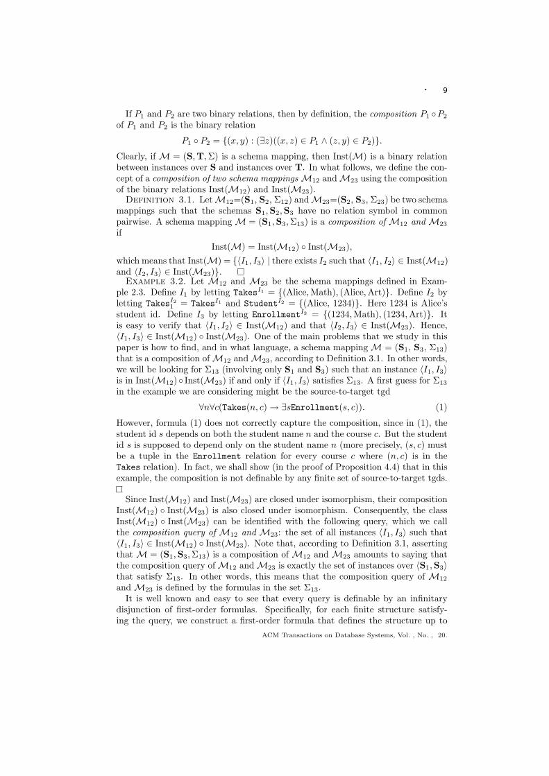
If P1 and P2 are two binary relations, then by definition, the composition P1 ◦P2

of P1 and P2 is the binary relation

P1 ◦ P2 = {(x, y) : (∃z)((x, z) ∈ P1 ∧ (z, y) ∈ P2)}.

Clearly, if M = (S,T,Σ) is a schema mapping, then Inst(M) is a binary relationbetween instances over S and instances over T. In what follows, we define the con-cept of a composition of two schema mappings M12 and M23 using the compositionof the binary relations Inst(M12) and Inst(M23).

Definition 3.1. LetM12=(S1, S2, Σ12) andM23=(S2, S3, Σ23) be two schemamappings such that the schemas S1,S2,S3 have no relation symbol in commonpairwise. A schema mapping M = (S1,S3,Σ13) is a composition of M12 and M23

ifInst(M) = Inst(M12) ◦ Inst(M23),

which means that Inst(M) = {〈I1, I3〉 | there exists I2 such that 〈I1, I2〉 ∈ Inst(M12)and 〈I2, I3〉 ∈ Inst(M23)}.

Example 3.2. Let M12 and M23 be the schema mappings defined in Exam-ple 2.3. Define I1 by letting TakesI1 = {(Alice,Math), (Alice,Art)}. Define I2 byletting TakesI2

1 = TakesI1 and StudentI2 = {(Alice, 1234)}. Here 1234 is Alice’sstudent id. Define I3 by letting EnrollmentI3 = {(1234,Math), (1234,Art)}. Itis easy to verify that 〈I1, I2〉 ∈ Inst(M12) and that 〈I2, I3〉 ∈ Inst(M23). Hence,〈I1, I3〉 ∈ Inst(M12) ◦ Inst(M23). One of the main problems that we study in thispaper is how to find, and in what language, a schema mapping M = (S1, S3, Σ13)that is a composition of M12 and M23, according to Definition 3.1. In other words,we will be looking for Σ13 (involving only S1 and S3) such that an instance 〈I1, I3〉is in Inst(M12)◦ Inst(M23) if and only if 〈I1, I3〉 satisfies Σ13. A first guess for Σ13

in the example we are considering might be the source-to-target tgd

∀n∀c(Takes(n, c) → ∃sEnrollment(s, c)). (1)

However, formula (1) does not correctly capture the composition, since in (1), thestudent id s depends on both the student name n and the course c. But the studentid s is supposed to depend only on the student name n (more precisely, (s, c) mustbe a tuple in the Enrollment relation for every course c where (n, c) is in theTakes relation). In fact, we shall show (in the proof of Proposition 4.4) that in thisexample, the composition is not definable by any finite set of source-to-target tgds.

Since Inst(M12) and Inst(M23) are closed under isomorphism, their compositionInst(M12) ◦ Inst(M23) is also closed under isomorphism. Consequently, the classInst(M12) ◦ Inst(M23) can be identified with the following query, which we callthe composition query of M12 and M23: the set of all instances 〈I1, I3〉 such that〈I1, I3〉 ∈ Inst(M12) ◦ Inst(M23). Note that, according to Definition 3.1, assertingthat M = (S1,S3,Σ13) is a composition of M12 and M23 amounts to saying thatthe composition query of M12 and M23 is exactly the set of instances over 〈S1,S3〉that satisfy Σ13. In other words, this means that the composition query of M12

and M23 is defined by the formulas in the set Σ13.It is well known and easy to see that every query is definable by an infinitary

disjunction of first-order formulas. Specifically, for each finite structure satisfy-ing the query, we construct a first-order formula that defines the structure up to


10 ·

isomorphism and then take the disjunction of all these formulas. This infinitaryformula defines the query. Moreover, every query is definable by a set of first-order formulas. Indeed, for each finite structure that does not satisfy the query, weconstruct the negation of the first-order formula that defines the structure up toisomorphism and then form the set of all such formulas. Note that this is an infi-nite set of first-order formulas, unless the query is satisfied by all but finitely manynon-isomorphic instances. This set is equivalent to its conjunction. Thus, everyquery is definable by an infinitary conjunction of first-order formulas. It followsthat a composition of two schema mappings always exists, since, given two schemamappings M12 and M23, we can obtain a composition M = (S1,S3,Σ13) of M12

and M23 by taking Σ13 to be the singleton consisting of an infinitary formula thatdefines the composition query of M12 and M23. Alternatively, we could take Σ13

to be the (usually infinite) set of first-order formulas that defines the compositionquery of M12 and M23. Since Σ13 defines the composition query, this compositionΣ13 is unique up to logical equivalence in the sense that if M = (S1, S3, Σ13) andM′ = (S1, S3, Σ′13) are both compositions of M12 and M23, then Σ13 and Σ′13 arelogically equivalent. For this reason, from now on we will refer to the compositionof M12 and M23, and will denote it by M12 ◦M23. We may also refer to Σ13 asthe composition of Σ12 and Σ23.

Since the composition query is always definable both by an infinitary formula andby an infinite set of first-order formulas, it is natural to investigate when the com-position of two schema mappings is definable in less expressive, but more tractable,logical formalisms. It is also natural to investigate whether the composition of twoschema mappings is definable in the same logical formalism that is used to definethese two schema mappings. We embark on this investigation in the next section.

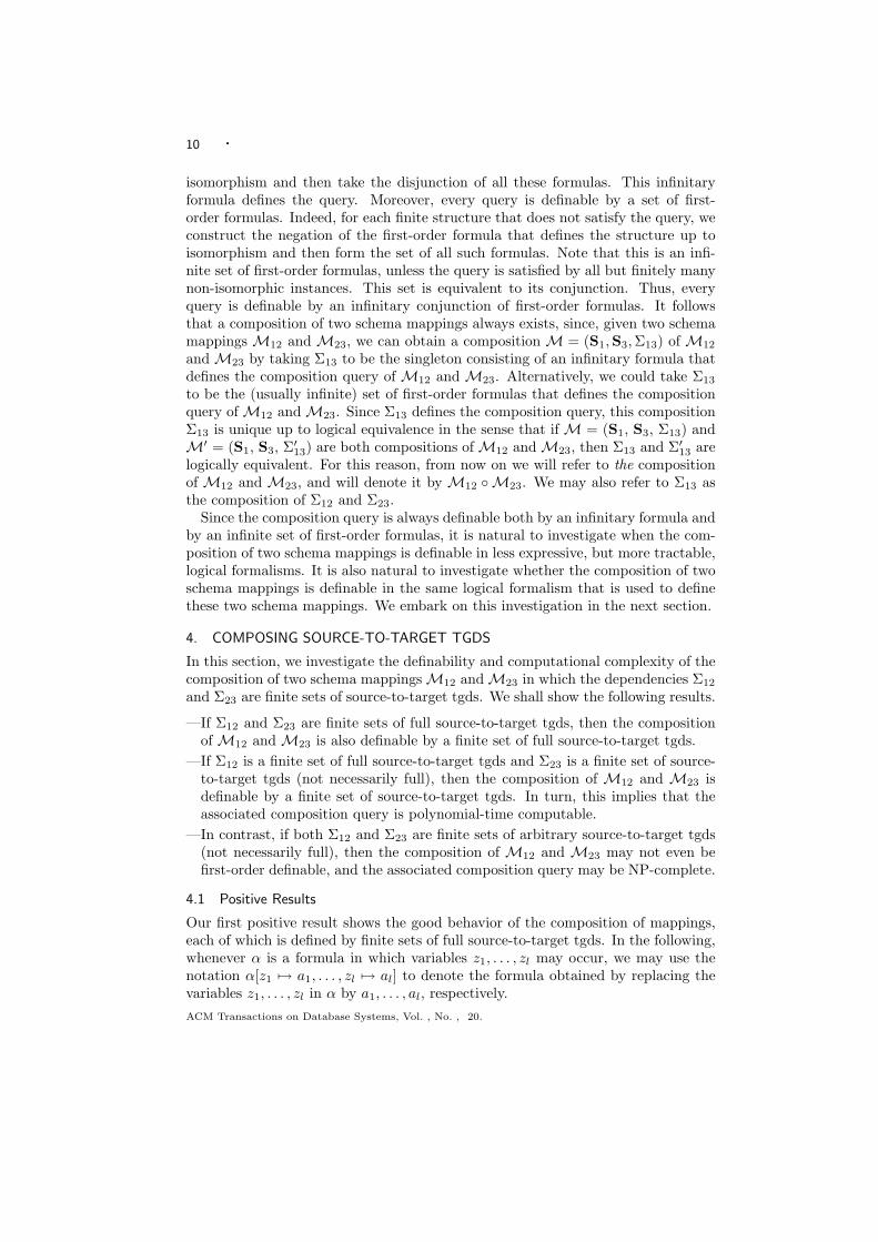
4. COMPOSING SOURCE-TO-TARGET TGDS

In this section, we investigate the definability and computational complexity of thecomposition of two schema mappings M12 and M23 in which the dependencies Σ12

and Σ23 are finite sets of source-to-target tgds. We shall show the following results.

—If Σ12 and Σ23 are finite sets of full source-to-target tgds, then the compositionof M12 and M23 is also definable by a finite set of full source-to-target tgds.

—If Σ12 is a finite set of full source-to-target tgds and Σ23 is a finite set of source-to-target tgds (not necessarily full), then the composition of M12 and M23 isdefinable by a finite set of source-to-target tgds. In turn, this implies that theassociated composition query is polynomial-time computable.

—In contrast, if both Σ12 and Σ23 are finite sets of arbitrary source-to-target tgds(not necessarily full), then the composition of M12 and M23 may not even befirst-order definable, and the associated composition query may be NP-complete.

4.1 Positive Results

Our first positive result shows the good behavior of the composition of mappings,each of which is defined by finite sets of full source-to-target tgds. In the following,whenever α is a formula in which variables z1, . . . , zl may occur, we may use thenotation α[z1 7→ a1, . . . , zl 7→ al] to denote the formula obtained by replacing thevariables z1, . . . , zl in α by a1, . . . , al, respectively.ACM Transactions on Database Systems, Vol. , No. , 20.

· 11

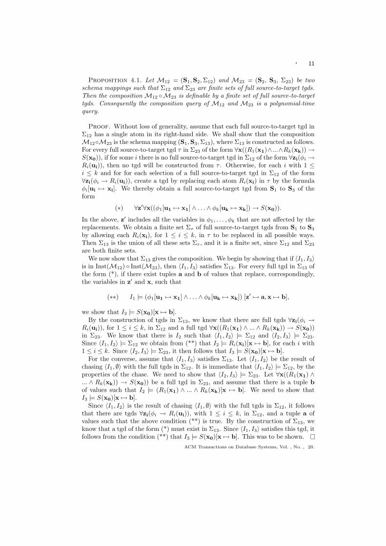
Proposition 4.1. Let M12 = (S1,S2,Σ12) and M23 = (S2, S3, Σ23) be twoschema mappings such that Σ12 and Σ23 are finite sets of full source-to-target tgds.Then the composition M12 ◦M23 is definable by a finite set of full source-to-targettgds. Consequently the composition query of M12 and M23 is a polynomial-timequery.

Proof. Without loss of generality, assume that each full source-to-target tgd inΣ12 has a single atom in its right-hand side. We shall show that the compositionM12◦M23 is the schema mapping (S1,S3,Σ13), where Σ13 is constructed as follows.For every full source-to-target tgd τ in Σ23 of the form ∀x((R1(x1)∧ ...∧Rk(xk)) →S(x0)), if for some i there is no full source-to-target tgd in Σ12 of the form ∀zi(φi →Ri(ui)), then no tgd will be constructed from τ . Otherwise, for each i with 1 ≤i ≤ k and for for each selection of a full source-to-target tgd in Σ12 of the form∀zi(φi → Ri(ui)), create a tgd by replacing each atom Ri(xi) in τ by the formulaφi[ui 7→ xi]. We thereby obtain a full source-to-target tgd from S1 to S3 of theform

(∗) ∀z′∀x((φ1[u1 7→ x1] ∧ . . . ∧ φk[uk 7→ xk]) → S(x0)).

In the above, z′ includes all the variables in φ1, . . . , φk that are not affected by thereplacements. We obtain a finite set Στ of full source-to-target tgds from S1 to S3

by allowing each Ri(xi), for 1 ≤ i ≤ k, in τ to be replaced in all possible ways.Then Σ13 is the union of all these sets Στ , and it is a finite set, since Σ12 and Σ23

are both finite sets.We now show that Σ13 gives the composition. We begin by showing that if 〈I1, I3〉

is in Inst(M12) ◦ Inst(M23), then 〈I1, I3〉 satisfies Σ13. For every full tgd in Σ13 ofthe form (*), if there exist tuples a and b of values that replace, correspondingly,the variables in z′ and x, such that

(∗∗) I1 |= (φ1[u1 7→ x1] ∧ . . . ∧ φk[uk 7→ xk]) [z′ 7→ a,x 7→ b],

we show that I3 |= S(x0)[x 7→ b].By the construction of tgds in Σ13, we know that there are full tgds ∀zi(φi →

Ri(ui)), for 1 ≤ i ≤ k, in Σ12 and a full tgd ∀x((R1(x1) ∧ ... ∧ Rk(xk)) → S(x0))in Σ23. We know that there is I2 such that 〈I1, I2〉 |= Σ12 and 〈I2, I3〉 |= Σ23.Since 〈I1, I2〉 |= Σ12 we obtain from (**) that I2 |= Ri(xi)[x 7→ b], for each i with1 ≤ i ≤ k. Since 〈I2, I3〉 |= Σ23, it then follows that I3 |= S(x0)[x 7→ b].

For the converse, assume that 〈I1, I3〉 satisfies Σ13. Let 〈I1, I2〉 be the result ofchasing 〈I1, ∅〉 with the full tgds in Σ12. It is immediate that 〈I1, I2〉 |= Σ12, by theproperties of the chase. We need to show that 〈I2, I3〉 |= Σ23. Let ∀x((R1(x1) ∧... ∧ Rk(xk)) → S(x0)) be a full tgd in Σ23, and assume that there is a tuple bof values such that I2 |= (R1(x1) ∧ ... ∧ Rk(xk)[x 7→ b]. We need to show thatI3 |= S(x0)[x 7→ b].

Since 〈I1, I2〉 is the result of chasing 〈I1, ∅〉 with the full tgds in Σ12, it followsthat there are tgds ∀zi(φi → Ri(ui)), with 1 ≤ i ≤ k, in Σ12, and a tuple a ofvalues such that the above condition (**) is true. By the construction of Σ13, weknow that a tgd of the form (*) must exist in Σ13. Since 〈I1, I3〉 satisfies this tgd, itfollows from the condition (**) that I3 |= S(x0)[x 7→ b]. This was to be shown.


12 ·

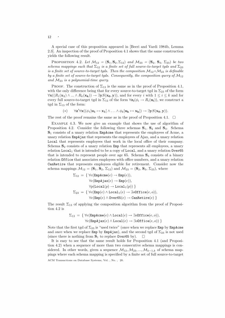
A special case of this proposition appeared in [Beeri and Vardi 1984b, Lemma2.3]. An inspection of the proof of Proposition 4.1 shows that the same constructionyields the following result.

Proposition 4.2. Let M12 = (S1,S2,Σ12) and M23 = (S2, S3, Σ23) be twoschema mappings such that Σ12 is a finite set of full source-to-target tgds and Σ23

is a finite set of source-to-target tgds. Then the composition M12 ◦M23 is definableby a finite set of source-to-target tgds. Consequently, the composition query of M12

and M23 is a polynomial-time query.

Proof. The construction of Σ13 is the same as in the proof of Proposition 4.1,with the only difference being that for every source-to-target tgd in Σ23 of the form∀x((R1(x1) ∧ ... ∧ Rk(xk)) → ∃yS(x0,y)), and for every i with 1 ≤ i ≤ k and forevery full source-to-target tgd in Σ12 of the form ∀zi(φi → Ri(ui)), we construct atgd in Σ13 of the form:

(∗) ∀z′∀x((φ1[u1 7→ x1] ∧ . . . ∧ φk[uk 7→ xk]) → ∃yS(x0,y)).

The rest of the proof remains the same as in the proof of Proposition 4.1.

Example 4.3. We now give an example that shows the use of algorithm ofProposition 4.2. Consider the following three schemas S1, S2 and S3. SchemaS1 consists of a unary relation EmpAcme that represents the employees of Acme, aunary relation EmpAjax that represents the employees of Ajax, and a unary relationLocal that represents employees that work in the local office of their company.Schema S2 consists of a unary relation Emp that represents all employees, a unaryrelation Local1 that is intended to be a copy of Local, and a unary relation Over65that is intended to represent people over age 65. Schema S3 consists of a binaryrelation Office that associates employees with office numbers, and a unary relationCanRetire that represents employees eligible for retirement. Consider now theschema mappings M12 = (S1, S2, Σ12) and M23 = (S2, S3, Σ23), where

Σ12 = { ∀e(EmpAcme(e) → Emp(e)),∀e(EmpAjax(e) → Emp(e)),∀p(Local(p) → Local1(p)) }

Σ23 = { ∀e(Emp(e) ∧ Local1(e) → ∃oOffice(e, o)),∀e(Emp(e) ∧ Over65(e) → CanRetire(e) }

The result Σ13 of applying the composition algorithm from the proof of Proposi-tion 4.2 is

Σ13 = { ∀e(EmpAcme(e) ∧ Local(e) → ∃oOffice(e, o)),∀e(EmpAjax(e) ∧ Local(e) → ∃oOffice(e, o)) }

Note that the first tgd of Σ23 is “used twice” (once when we replace Emp by EmpAcmeand once when we replace Emp by EmpAjax), and the second tgd of Σ23 is not used(since there is nothing from S1 to replace Over65 by).

It is easy to see that the same result holds for Proposition 4.1 (and Proposi-tion 4.2) when a sequence of more than two consecutive schema mappings is con-sidered. In other words, given a sequence M12,M23, ...,Mk−1,k of schema map-pings where each schema mapping is specified by a finite set of full source-to-targetACM Transactions on Database Systems, Vol. , No. , 20.

· 13

tgds, the composition M12 ◦ · · · ◦ Mk−1,k is also definable by a finite set of fullsource-to-target tgds. If the last schema mapping Mk−1,k is specified by a finiteset of source-to-target tgds and all of the others are specified by a finite set of fullsource-to-target tgds, then the composition M12 ◦ ... ◦ Mk−1,k is definable by afinite set of source-to-target tgds.

4.2 Negative Results

We now present a series of negative results associated with the composition ofschema mappings specified by source-to-target tgds.

Proposition 4.4. There exist schema mappings M12 = (S1, S2, Σ12) andM23 = (S2, S3, Σ23) such that Σ12 is a finite set of source-to-target tgds, Σ23

is a finite set of full source-to-target tgds, and the following hold for the composi-tion M12 ◦M23:1. M12 ◦ M23 is not definable by any finite set of source-to-target tgds, but it is

definable by an infinite set of source-to-target tgds.2. M12 ◦M23 is definable by a first-order formula. Consequently, the composition

query of M12 and M23 is a polynomial-time query.

Proof. The two schema mappings that we use to prove the proposition are theschema mappings M12 and M23 of Example 2.3. Assume that according to theinstance I1, a student with name n is taking courses c1, . . . , ck. According to thesecond tgd of Σ12, this student n is assigned (at least one) student id s. Accordingto Σ23, the instance I3 then contains tuples (s, c1), . . . , (s, ck). These requirementsare described by the following source-to-target tgd, which we denote by φk:

∀n∀c1 . . .∀ck(Takes(n, c1) ∧ . . . ∧ Takes(n, ck) →∃s(Enrollment(s, c1) ∧ . . . ∧ Enrollment(s, ck)))

We next show that the composition M12 ◦M23 is given by M = (S1,S3,Σ13),where Σ13 is the infinite set {φ1, . . . , φk, . . .} of source-to-target tgds.

Assume first that 〈I1, I3〉 ∈ Inst(M12) ◦ Inst(M23). This means that there is I2over S2 such that 〈I1, I2〉 |= Σ12 and 〈I2, I3〉 |= Σ23. We need to show that 〈I1, I3〉 |=φk, for each k ≥ 1. Assume that TakesI1 contains tuples (n, c1), . . . , (n, ck), wheren is a concrete student name, and c1, . . . , ck are concrete courses. Since 〈I1, I2〉 |=Σ12, we obtain that TakesI2

1 contains the tuples (n, c1), . . . , (n, ck) and StudentI2

contains the tuple (n, s), for some value s. Since 〈I2, I3〉 |= Σ23, we then obtainthat EnrollmentI3 contains the tuples (s, c1), . . . , (s, ck). Hence, 〈I1, I3〉 |= φk.

Conversely, assume that 〈I1, I3〉 |= φk, for each k ≥ 1. We need to show that thereis I2 such that 〈I1, I2〉 |= Σ12 and 〈I2, I3〉 |= Σ23. We construct I2 as follows. We letStudentI2 be the set of all tuples (n, s) such that: (1) some tuple (n, c) occurs inTakesI1 , (2) the set {c1, . . . , cl} is the set of all courses c such that (n, c) appears inTakesI1 , and (3) s is such that EnrollmentI3 contains the tuples (s, c1), . . . , (s, cl).We note that s as in condition (3) must exist, whenever TakesI1 contains tuples(n, c1), . . . , (n, cl). This is due to the fact that 〈I1, I3〉 satisfies φl. Furthermore, welet TakesI2

1 = TakesI1 . It is immediate that 〈I1, I2〉 |= Σ12.We now show that 〈I2, I3〉 |= Σ23. Indeed, assume that StudentI2 contains a

tuple (n, s), and that TakesI21 contains a tuple (n, c); we must show that the tuple


14 ·

(s, c) is in EnrollmentI3 . By construction of TakesI21 , we know that (n, c) is in

TakesI1 . Let {c1, . . . , cl} be the set of all courses c′ such that (n, c′) is in TakesI1 ;this set certainly contains c. By construction of StudentI2 , we know that s hasthe property that EnrollmentI3 contains the tuples (s, c1), . . . , (s, cl). Since c is amember of {c1, . . . , cl}, it follows that the tuple (s, c) is in EnrollmentI3 , as desired.

It can be verified that Σ13 is not equivalent to any finite subset of it. We nowshow that, in fact, Σ13 is not equivalent to any finite set of source-to-target tgds.The proof of this uses the chase as well as the concept of universal solution. Supposethere is a finite set Σfin

13 of source-to-target tgds that is logically equivalent to Σ13.Let Mfin = (S1,S3,Σfin

13 ) and consider the following source instance I1:

TakesI1 = {(n, c1), . . . , (n, cm)}

where n is some student name and c1, . . . , cm are the courses that this studenttakes. We assume that m is a large enough number, that we shall specify shortly.

We construct an instance I3 over S3, by chasing (as in [Fagin, Kolaitis, Millerand Popa 2005]) the instance 〈I1, ∅〉 with the source-to-target tgds in Σfin

13 , where ∅is an empty instance. The chase applies the source-to-target tgds in Σfin

13 and addsinto I3 all the necessary tuples whenever it finds a source-to-target tgd that is notsatisfied. This is repeated until all the source-to-target tgds are satisfied. Note thatthe chase terminates, since we are chasing with xource-to-target tgds. New values,also called nulls, different from the source values in I1 and different from any othervalues that may have been added earlier, may appear as part of the tuples addedin a chase step with a source-to-target tgd. These nulls are used to replace theexistentially quantified variables. Since I3 is the result of the chase, it follows froma theorem in [Fagin, Kolaitis, Miller and Popa 2005] that I3 is a universal solutionof I1 under Mfin.

In particular, I3 is solution of I1 under Mfin, that is, 〈I1, I3〉 |= Σfin13 . Since

Σfin13 and Σ13 are equivalent, we have that 〈I1, I3〉 |= Σ13, and in particular,

〈I1, I3〉 |= φm. It follows that EnrollmentI3 must contain a set of tuples of the form(s, c1), . . . , (s, cm) for some value s. We now show that s cannot appear among thevalues of I1. In other words, we show that s must be a null. For this, we use thefact that I3 is universal.

Consider the following instance V over S3: EnrollmentV = {(S, c1), . . . , (S, cm)}where S is a null representing a student id. It is easy to see that 〈I1, V 〉 |= Σ13.Since Σfin

13 and Σ13 are equivalent, it follows that 〈I1, V 〉 |= Σfin13 and, hence, V is a

solution for I1 under Mfin. Since I3 is a universal solution for I1 under Mfin, theremust exist a homomorphism h from I3 to V such that h(v) = v for every sourcevalue v. But every homomorphism from I3 to V is forced to map s into the null S.Hence, s cannot be a source value (or, otherwise, h(s) would have to be s). Thus,we showed that EnrollmentI3 contains a set {(s, c1), . . . , (s, cm)} of tuples where sis a null.

Let l be the maximum number of atoms that are under the scope of existentialquantifiers in any source-to-target tgd in Σfin

13 . Since I3 is the result of the chasewith Σfin

13 , it follows that a null in I3 can occur in at most l tuples. However, ifwe take m to be larger than l, then the above obtained set {(s, c1), . . . , (s, cm)} oftuples gives a contradiction. Therefore, Σ13 is not logically equivalent to any finiteACM Transactions on Database Systems, Vol. , No. , 20.

· 15

set of source-to-target tgds.Finally, the composition M12 ◦M23 of the two schema mappings is definable by

the first-order formula ∀n∃s∀c(Takes(n, c) → Enrollment(s, c)). We shall verifythis in Example 5.1, where we show that a logically equivalent formula defines thecomposition.

It is an interesting open problem to consider the complexity of deciding, givenschema mappings M12 and M23, each defined by finite sets of source-to-target tgds,whether the composition M12 ◦M23 is definable by a finite set of source-to-targettgds. In particular, it is not even clear whether this problem is decidable.

We have just given an example in which the composition is definable by an infiniteset of source-to-target tgds, but it is not definable by any finite set of source-to-target tgds. There is also a different example in which the composition is notdefinable even by an infinite set of source-to-target tgds. This is stated in thenext result, which amplifies the limitations of the language of source-to-target tgdswith respect to composition. A proof appears in Section 5.1, after we develop thenecessary machinery.

Proposition 4.5. There exist schema mappings M12 = (S1, S2, Σ12) andM23 = (S2, S3, Σ23) such that Σ12 consists of a single source-to-target tgd, Σ23 isa finite set of full source-to-target tgds, and the composition M12 ◦M23 cannot bedefined by any finite or infinite set of source-to-target tgds.

In the example given in Proposition 4.4, the composition query is polynomial-time computable, since it is first-order. In what follows, we will show that thereare schema mappings M12 and M23 such that Σ12 is a finite set of source-to-targettgds, Σ23 consists of a single full source-to-target tgd, but the composition query forM12◦M23 is NP-complete. Furthermore, this composition query is not definable byany formula of the finite-variable infinitary logic Lω

∞ω, which is a powerful formalismthat subsumes least fixed-point logic LFP (hence, it subsumes first-order logic andDatalog) on finite structures (see [Abiteboul, Hull and Vianu 1995]).

Theorem 4.6. There exist schema mappings M12 = (S1, S2, Σ12) and M23 =(S2, S3, Σ23) such that Σ12 is a finite set of source-to-target tgds, each having atmost one existential quantifier, Σ23 consists of one full source-to-target tgd, andsuch that the following hold for the composition M12 ◦M23:1. The composition query of M12 and M23 is NP-complete.2. The composition M12 ◦M23 is not definable by any formula of Lω

∞ω, and henceof least fixed-point logic LFP.

Proof. Later (Proposition 4.8), we shall show that the composition query ofschema mappings definable by finite sets of source-to-target tgds is always in NP. Aswe now describe, NP-hardness can be obtained by a reduction of 3-Colorabilityto the composition query of two fixed schema mappings. The schema S1 consistsof a single binary relation symbol E, the schema S2 consists of two binary relationsymbols C and F , and the schema S3 consists of one binary relation symbol D.The set Σ12 consists of the following three source-to-target tgds:

∀x∀y(E(x, y) → ∃uC(x, u))ACM Transactions on Database Systems, Vol. , No. , 20.

16 ·

∀x∀y(E(x, y) → ∃uC(y, u))∀x∀y(E(x, y) → F (x, y)).

Intuitively, C(x, u) means that node x has color u. The third tgd of Σ12 intuitivelycopies the edge relation E into the relation F . Finally, Σ23 consists of a single fullsource-to-target tgd:

∀x∀y∀u∀v(C(x, u) ∧ C(y, v) ∧ F (x, y) → D(u, v)).

Intuitively, this tgd says that if u and v are the colors of adjacent nodes, then thetuple (u, v) is in the “distinctness” relation D, which we shall take to consist oftuples of distinct colors. Thus, if u and v are the colors of adjacent nodes, then weare forcing u and v to be distinct colors.

Let I3 be the instance over the schema S3 with

DI3 = {(r, g), (g, r), (b, r), (r, b), (g, b), (b, g)}.

In words, DI3 contains all pairs of different colors among the three colors r, g, and b.Let G = (V,E) be a graph and let I1 be the instance over S1 consisting of the edgerelation E of G. We claim that G is 3-colorable if and only if 〈I1, I3〉 ∈ Inst(M12)◦Inst(M23). This is sufficient to prove the theorem, since 3-Colorability is NP-complete [Garey, Johnson and Stockmeyer 1976].

If G is 3-colorable, then there is a function c from V to the set {r, b, g} such thatfor every edge (x, y) ∈ E, we have that c(x) 6= c(y). Let I2 be the instance overS2 with CI2 = {(x, c(x)) : x ∈ V } and F I2 = E. Clearly, 〈I1, I2〉 ∈ Inst(M12) and〈I2, I3〉 ∈ Inst(M23). Therefore, 〈I1, I3〉 ∈ Inst(M12) ◦ Inst(M23).

Conversely, assume that 〈I1, I3〉 is in Inst(M12) ◦ Inst(M23). This means thereexists an instance I2 over S2 such that 〈I1, I2〉 ∈ Inst(M12) and 〈I2, I3〉 ∈ Inst(M23).The first two source-to-target tgds in Σ12 state that for each node n incident to anedge there exists some u such that C(n, u), while the third source-to-target tgd inΣ12 asserts that the edge relation E is contained in F I2 . We construct a coloringfunction c as follows. For each node n that is incident to an edge we take c(n) = u,where u is picked arbitrarily among those u that satisfy C(n, u). Since DI3 is theinequality relation on {r, g, b}, the full source-to-target tgd in Σ23 enforces that forevery edge of G, and no matter which u we picked for a given n, the two vertices ofthat edge are assigned different colors among the three colors r, g and b. Therefore,G is 3-colorable, as desired.

The above reduction of 3-Colorability to the composition query of M12 andM23 belongs to a class of weak polynomial-time reductions known as quantifier-freereductions, since the instance 〈I1, I3〉 of the composition query can be defined fromthe instance G = (V,E) using quantifier-free formulas (see [Immerman 1999] forthe precise definitions). Dawar [Dawar 1998] showed that 3-Colorability is notexpressible in the finite-variable infinitary logic Lω

∞ω. Since definability in Lω∞ω is

preserved under quantifier-free reductions, it follows that the composition query ofM12 and M23 is not expressible in Lω

∞ω. In turn, this implies that the compositionquery of M12 and M23 is not expressible in least fixed-point logic LFP, sinceLω∞ω subsumes LFP on the class of all finite structures (see [Ebbinghaus and Flum

1999]).ACM Transactions on Database Systems, Vol. , No. , 20.

· 17

Proposition 4.2 and Theorem 4.6 yield a sharp boundary on the definability ofthe composition of schema mappings specified by finite sets of source-to-target tgds.Specifically, the composition of a finite set of full source-to-target tgds with a finiteset of source-to-target tgds is always definable by a first-order formula (and, in fact,definable by a finite conjunction of source-to-target tgds), while the composition ofa finite set of source-to-target tgds, each having at most one existential quantifier,with a set consisting of one full source-to-target tgd may not even be Lω

∞ω-definable.Similarly, the computational complexity of the associated composition query mayjump from solvable in polynomial time to NP-complete.

The Homomorphism Problem over the schema S is the following decisionproblem: given two instances I and J of S, is there a homomorphism from Ito J? (Recall that a homomorphism from I to J is a function h such that forevery relation symbol R in S and every tuple (a1, . . . , an) ∈ RI , we have that(h(a1), . . . , h(an)) ∈ RJ .) This is a fundamental algorithmic problem because,as shown by Feder and Vardi [Feder and Vardi 1998], all constraint satisfactionproblems can be identified with homomorphism problems. In particular, 3-Sat and3-Colorability are special cases of the Homomorphism Problem over suitableschemas. For instance, 3-Colorability amounts to the following problem: givena graph G, is there a homomorphism from G to the complete 3-node graph K3?A slight modification of the proof of the preceding Theorem 4.6 shows that forevery schema S, the Homomorphism Problem over S has a simple quantifier-freereduction to the composition query of two schema mappings specified by finite setsof source-to-target tgds.

Proposition 4.7. For every schema S = 〈R1, . . . , Rm〉, there are schema map-pings M12 = (S1, S2, Σ12) and M23 = (S2, S3, Σ23) such that Σ12 is a finite setof source-to-target tgds and Σ23 is a finite set of full source-to-target tgds, with theproperty that the Homomorphism Problem over S has a quantifier-free reductionto the composition query of M12 and M23.

Proof. The schema S1 is the same as the schema S = 〈R1, . . . , Rm〉. Theschema S2 is 〈H,T1, ..., Tm〉, where H is a binary relation symbol and each Ti hasthe same arity as Ri, for 1 ≤ i ≤ m. The schema S3 is 〈P1, . . . , Pm〉, where eachPi has the same arity as Ri, for 1 ≤ i ≤ m. The dependencies in Σ12 and Σ23 areas follows:

Σ12 = { ∀x1...∀xk1(R1(x1, ..., xk1) → ∃y1...∃yk1 (H(x1, y1) ∧ ... ∧H(xk1 , yk1))),...∀x1...∀xkm

(Rm(x1, ..., xkm) → ∃y1...∃ykm

(H(x1, y1) ∧ ... ∧H(xkm, ykm

))),∀x(R1(x) → T1(x)),...∀x(Rm(x) → Tm(x)) }

Σ23 = { ∀x1∀y1...∀xk1∀yk1

((H(x1, y1) ∧ ... ∧H(xk1 , yk1) ∧T1(x1, ..., xk1)) → P1(y1, ..., yk1)),...∀x1∀y1...∀xkm

∀ykm


18 ·

((H(x1, y1) ∧ ... ∧H(xkm, ykm

) ∧Tm(x1, ..., xkm)) → Pm(y1, ..., ykm

)) }.

Intuitively, the Ri relation is being copied into the Ti relation, for 1 ≤ i ≤ m,and H(x, y) means that a homomorphism is mapping x to y.

Let I = 〈RI1, ..., R

Im〉 and J = 〈RJ

1 , . . . , RJm〉 be two instances of S. Since S1 is

the same as S, we have that I is an instance of S1. Let J ′ be the instance overS3 where P J′

i = RJi , for 1 ≤ i ≤ m. (Thus, J ′ is the same as J except that the

relation names reflect schema S3 rather than S1.) It is easy to verify that there isa homomorphism from I to J if and only if 〈I, J ′〉 is in Inst(M12) ◦ Inst(M23).

The next result establishes an upper bound on the computational complexity ofthe composition query associated with two schema mappings specified by finite setsof source-to-target tgds. It also shows that the composition of two such mappingsis always definable by an existential second-order formula.

Proposition 4.8. If M12 = (S1,S2,Σ12) and M23 = (S2, S3, Σ23) are schemamappings such that Σ12 and Σ23 are finite sets of source-to-target tgds, then thecomposition query of M12 and M23 is in NP. Consequently, the composition M12◦M23 is definable by an existential second-order formula.

Proof. To establish membership in NP, it suffices to show that if 〈I1, I3〉 ∈Inst(M12)◦Inst(M23), then there is an instance I2 over S2 that has size polynomialin the sizes of I1 and I3, and is such that 〈I1, I2〉 |= Σ12 and 〈I2, I3〉 |= Σ23.

Suppose we have I1 and I3 as above. Then there is an instance J such that〈I1, J〉 |= Σ12 and 〈J, I3〉 |= Σ23. Since Σ12 is a set of source-to-target tgds, theschema mapping M12 is a data exchange setting with source S1 and target S2

(and no target dependencies). Moreover, by results of [Fagin, Kolaitis, Miller andPopa 2005], in this data exchange setting there is a universal solution U for I1 ofsize polynomial in the size of I1. By definition, a universal solution U for I1 hasthe property that, for every solution for I1, there is a homomorphism h from U tothat solution such that h is the identity on values from I1. In particular, there isa homomorphism h : U → J such that h(v) = v, for every value v from I1. LetI2 = h(U). Clearly, I2 is an instance over S2, has size at most the size of U , and is asubinstance of J . Since (a) Σ12 is a set of source-to-target tgds, (b) 〈I1, U〉 |= Σ12,and (c) h is a homomorphism from U to I2 that is the identity on values from I1,we have that 〈I1, I2〉 |= Σ12. Furthermore, since (a) Σ23 is a set of source-to-targettgds, (b) 〈J, I3〉 |= Σ23, and (c) I2 is a subinstance of J , we have that 〈I2, I3〉 |= Σ23.

The fact that the composition query of M12 and M23 is in NP implies, by Fagin’sTheorem [Fagin 1974], that the composition M12 ◦M23 is definable on instances〈I1, I3〉 over 〈S1,S3〉 by an existential second-order formula, where the existentialsecond-order variables are interpreted over relations on the union of the set of valuesin I1 with the set of values in I3.

We conclude this section by showing that the results of Proposition 4.8 may faildramatically for schema mappings specified by arbitrary first-order formulas.

Proposition 4.9. There are schema mappings M12 = (S1, S2, Σ12) and M23 =(S2,S3,Σ23) such that Σ12 consists of a single first-order formula, Σ23 is the emptyset, and the composition query of M12 and M23 is undecidable.


· 19

Proof. We define M12 in such a way that 〈I1, I2〉 ∈ Inst(M12) precisely when I1is the encoding of a Turing machine and I2 represents a terminating computation ofthat Turing machine (thus, Σ12 consists of a first-order formula that expresses thisconnection). We let the schema S3 consist of, say, a single unary relation symbol,and let Σ23 be the empty set. So, the composition M12 ◦M23 consists of all 〈I1, I3〉where I1 is the encoding of a halting Turing machine, and I3 is arbitrary. Theresult follows from the fact that it is undecidable to determine if a Turing machineis halting.

5. SECOND-ORDER TGDS

We have seen in the previous section that the composition of two schema map-pings specified by finite sets of source-to-target tgds may not be definable by aset (finite or infinite) of source-to-target tgds. From Proposition 4.8, however, weknow that such a composition is always definable by an existential second-orderformula. We shall show in this section that, in fact, the composition of schemamappings, each specified by a finite set of source-to-target tgds, is always definableby a restricted form of existential second-order formula, which we call a second-ordertuple-generating dependency (SO tgd). Intuitively, an SO tgd is a source-to-targettgd suitably extended with existentially quantified functions and with equalities.Every finite set of source-to-target tgds is equivalent to an SO tgd. Furthermore,an SO tgd is capable of defining the composition of two schema mappings thatare specified by SO tgds. In other words, SO tgds are closed under composition.Moreover, we shall show in Section 6 that SO tgds possess good properties for dataexchange. All these properties justify SO tgds as the right language for representingschema mappings and for composing schema mappings.

Example 5.1. The proof of Proposition 4.4 shows that for the two schemamappings of Example 2.3 there is no finite set of source-to-target tgds that candefine the composition. At the end of the proof of Proposition 4.4, it was notedthat the composition is defined by the first-order formula ∀n∃s∀c(Takes(n, c) →Enrollment(s, c)). If we Skolemize this formula, we obtain the following formula,which is an SO tgd that defines the composition:

∃f( ∀n∀c (Takes(n, c) → Enrollment(f(n), c)) ) (2)

In this formula, f is a function symbol that associates each student name n with astudent id f(n). The SO tgd states that whenever a student name n is associatedwith a course c in Takes, then the corresponding student id f(n) is associated with cin Enrollment. This is independent of how many courses a student takes: if studentname n is associated with courses c1, . . . , ck in Takes, then f(n) is associated withall of c1, . . . , ck in Enrollment.

We now verify that (2) does indeed define the composition. Assume first that〈I1, I3〉 ∈ Inst(M12) ◦ Inst(M23). Then there is I2 over S2 such that 〈I1, I2〉 |= Σ12

and 〈I2, I3〉 |= Σ23. We construct a function f0 as follows. For each n such that(n, c) is in TakesI1 , we set f0(n) = s, where s is such that (n, s) is in StudentI2

(such s is guaranteed to exist according to the second source-to-target tgd in Σ12,and we pick one such s). It is immediate that 〈I1, I3〉 satisfies the SO tgd when theexistentially quantified function symbol f is instantiated with the constructed f0.Conversely, assume that 〈I1, I3〉 satisfies the SO tgd. Then there is a function f0


20 ·

such that for every (n, c) in TakesI1 we have that (f0(n), c) is in EnrollmentI3 . LetI2 be such that StudentI2 = {(n, f0(n) | (n, c) ∈ TakesI1} and TakesI2

1 = TakesI1 .It can be verified that 〈I1, I2〉 |= Σ12 and 〈I2, I3〉 |= Σ23.

Example 5.2. This example illustrates a slightly more complex form of a second-order tgd that contains equalities between terms. Consider the following threeschemas S1, S2 and S3. Schema S1 consists of a single unary relation symbol Empof employees. Schema S2 consists of a single binary relation symbol Mgr1, thatassociates each employee with a manager. Schema S3 consists of a similar binaryrelation symbol Mgr, that is intended to provide a copy of Mgr1. and an addi-tional unary relation symbol SelfMgr, that is intended to store employees who aretheir own manager. Consider now the schema mappings M12 = (S1, S2,Σ12) andM23 = (S2,S3,Σ23), where

Σ12 = { ∀e (Emp(e) → ∃mMgr1(e,m)) } Σ23 = { ∀e∀m (Mgr1(e,m) → Mgr(e,m)),∀e(Mgr1(e, e) → SelfMgr(e)) }.

It is straightforward to verify that the composition of M12 and M23 is M13, whereΣ13 is the following second-order tgd:

∃f( ∀e(Emp(e) → Mgr(e, f(e))) ∧∀e(Emp(e) ∧ (e = f(e)) → SelfMgr(e))).

In fact, we shall derive this later when we give a composition algorithm.We will use this example in Section 5.1 to show that equalities in SO tgds are

strictly necessary for the purposes of composition, and also to give a proof for theearlier Proposition 4.5.

Before we formally define SO tgds, we need to define terms. Given a collectionx of variables and a collection f of function symbols, a term (based on x and f) isdefined recursively as follows:

1. Every variable in x is a term.2. If f is a k-ary function symbol in f and t1, . . . , tk are terms, then f(t1, . . . , tk)

is a term.

We now give the precise definition of an SO tgd.3Definition 5.3. Let S be a source schema and T a target schema. A second-

order tuple-generating dependency (SO tgd) is a formula of the form:

∃f((∀x1(φ1 → ψ1)) ∧ ... ∧ (∀xn(φn → ψn))), (3)

where

1. Each member of f is a function symbol.2. Each φi is a conjunction of• atomic formulas of the form S(y1, ..., yk), where S is a k-ary relation symbol ofschema S and y1, . . . , yk are variables in xi, not necessarily distinct,and• equalities of the form t = t′ where t and t′ are terms based on xi and f .

3This definition is slightly different from that given in our conference version [Fagin, Kolaitis,

Popa and Tan 2004]. Every SO tgd as defined here is an SO tgd as defined in [Fagin, Kolaitis,

Popa and Tan 2004], but not conversely. However, every SO tgd as defined in [Fagin, Kolaitis,Popa and Tan 2004] is logically equivalent to an SO tgd as defined here.


· 21

3. Each ψi is a conjunction of atomic formulas T (t1, ..., tl), where T is an l-aryrelation symbol of schema T and t1, . . . , tl are terms based on xi and f .

4. Each variable in xi appears in some atomic formula of φi.We may refer to each subformula ∀xi(φi → ψi) as a conjunct of the second-order

tgd; we may also use the shorthand notation Ci for this conjunct.The fourth condition is a “safety” condition, analogous to that made for (first-

order) source-to-target tgds. As an example, the following formula is not a validsecond-order tgd:

∃f∃g∀x∀y(S(x) ∧ (g(y) = f(x)) → T (x, y)).

The safety condition is violated, since the variable y does not appear in an atomicformula on the left-hand side.

There is a subtlety in the definition of SO tgds, namely, the semantics of existen-tialized function symbols.4 What should the domain and range of the correspondingfunctions be? Thus, if we are trying to evaluate whether the SO tgd (3) is satisfiedby 〈I, J〉, what should the domain and range be for the concrete functions thatmay replace the existentialized function symbols in f? Perhaps the most obviouschoice is to let the domain and range be the active domain of 〈I, J〉 (the active do-main of 〈I, J〉 consists of those values that appear in I and/or J). In the proof ofProposition 4.8, the existential second-order variables are interpreted over relationson the active domain. But as we shall see in Section 7.3, this choice of the activedomain as the universe may give us the “wrong answer”. Intuitively, if our instance〈I, J〉 is 〈I1, I3〉, we may wish the functions to take on values in the “missing middleinstance” I2, which may be much bigger than I1 and I3.

We define the semantics by converting each instance 〈I, J〉 into a structure〈U ; I, J〉, which is just like 〈I, J〉 except that it has a universe U . The domainand range of the functions is then taken to be U . We take the universe U to bea countably infinite set that includes the active domain. The intuition is that theuniverse contains the active domain along with an infinite set of nulls. Then, if σis an SO tgd, we define 〈I, J〉 |= σ to hold precisely if 〈U ; I, J〉 |= σ under the stan-dard notion of satisfaction in second-order logic (see, for example, [Ebbinghaus andFlum 1999] or [Enderton 2001]). The standard notion of satisfaction says that if σis ∃fσ′, where σ′ is first-order, then 〈U ; I, J〉 |= σ precisely if there is a collectionf0 of functions with domain and range U such that 〈U ; I, J〉 satisfies σ′ when eachfunction symbol in f is replaced by the corresponding function in f0. We may write〈U ; I, J〉 |= σ′[f 7→ f0] to represent this situation, or simply 〈I, J〉 |= σ′[f 7→ f0]when the universe U is fixed and understood from the context. As we shall see inSection 5.2, instead of taking the universe U to be infinite, we can take it to befinite and “sufficiently large”.

Several remarks are in order now. First, SO tgds are closed under conjunction.That is, if σ1 and σ2 are SO tgds, then the conjunction σ1∧σ2 is logically equivalentto an SO tgd. This is because we simply rename the function symbols in σ2 to bedisjoint from those in σ1; then, if σ1 is ∃f1σ′1, and σ2 is ∃f2σ′2, with f1 and f2 disjoint,the conjunction ∃f1σ′1 ∧ ∃f2σ′2 is logically equivalent to ∃f1∃f2(σ′1 ∧ σ′2). Of course,

4This subtlety was pointed out to us by Sergey Melnik, in the context of domain independence(which we shall discuss in Section 5.2).


22 ·

the fact that SO tgds are closed under conjunction implies that every finite set ofSO tgds is logically equivalent to a single SO tgd. For this reason, when we considerschema mappings specified by SO tgds, it is enough to restrict our attention to thecase where the set Σst consists of one SO tgd. We will then identify the singletonset Σst with the SO tgd itself, and refer to Σst as an SO tgd.

Second, it should not come as a surprise that every (first-order) source-to-targettgd is equivalent to an SO tgd. In fact, it is easy to see that every source-to-target tgd is equivalent to an SO tgd without equalities. Specifically, let σ be thesource-to-target tgd

∀x1 . . .∀xm(φS(x1, . . . , xm) → ∃y1 . . .∃ynψT (x1, . . . , xm, y1, . . . , yn)).Then σ is equivalent to the following SO tgd without equalities, which is obtainedby Skolemizing σ:

∃f1 . . .∃fn∀x1 . . .∀xm(φS(x1, . . . , xm) →ψT (x1, . . . , xm, f1(x1, . . . , xm), . . . , fn(x1, . . . , xm))).

Given a finite set Σ of source-to-target tgds, we can find an SO tgd that is equiv-alent to Σ by taking, for each tgd σ in Σ, a conjunct of the SO tgd to capture σas described above (we use disjoint sets of function symbols in each conjunct, asbefore).

Third, we point out that every SO tgd is equivalent to an SO tgd in a “normalform” where the right-hand sides (that is, the formulas ψi in (3)) are atomic for-mulas, rather than conjunctions of atomic formulas. For example, consider the SOtgd

∃f∀x(R(x) → (S(x, f(x)) ∧ T (f(x), x))).

This SO tgd is logically equivalent to the SO tgd

∃f(∀x(R(x) → S(x, f(x))) ∧ ∀x(R(x) → T (f(x), x))).

This is unlike the situation for (first-order) source-to-target dependencies, wherewe would lose expressive power if we required that the right-hand sides consist onlyof atomic formulas and not conjunctions of atomic formulas. In our compositionalgorithm that we shall present in Section 7, we begin by converting SO tgds tothis normal form.

The next three subsections delve into further details on second-order tgds. Wefirst show that equalities are strictly needed in the definition of SO tgds (or else welose expressive power). We then show that the choice of the universe for SO tgdsdoes not really matter, as long as the universe contains the active domain and issufficiently large. The section concludes with a consideration of the model-checkingproblem and how it differs from the first-order case.

5.1 The Necessity of Equalities in Second-Order TGDs

Our definition of SO tgds allows for equalities between terms in the formulas φi,even though we just saw that SO tgds that represent first-order tgds do not requireequalities. The next theorem (or its corollary) tells us that such equalities arenecessary, since it may not be possible to define the composition of two schemamappings otherwise. This theorem is stated in more generality than simply sayingthat equalities are necessary, in order to provide a proof of Proposition 4.5.


· 23

Theorem 5.4. There exist schema mappings M12 = (S1, S2, Σ12) and M23 =(S2, S3, Σ23) where Σ12 consists of a single source-to-target tgd, Σ23 is a finiteset of full source-to-target tgds, and the composition M12 ◦M23 is given by an SOtgd that is not logically equivalent to any finite or infinite set of SO tgds withoutequalities.

Proof. Let S1, S2, S3, Σ12, Σ23, and Σ13 be as in Example 5.2. We need onlyshow that there is no finite or infinite set of SO tgds without equalities that islogically equivalent to Σ13.

Define I1 by letting EmpI1 = {Bob}. Define I3 by letting MgrI3 = {(Bob,Susan)}and SelfMgrI3 = ∅. Define I ′3 by letting MgrI′

3 = {(Bob,Bob)} and SelfMgrI′3 = ∅.

It is easy to see that 〈I1, I3〉 |= Σ13; intuitively, we let f(Bob) = Susan. It is alsoeasy to see that 〈I1, I ′3〉 6|= Σ13, since SelfMgrI′

3 does not contain Bob.We shall show that every SO tgd without equalities that is satisfied by 〈I1, I3〉

is also satisfied by 〈I1, I ′3〉. Since also 〈I1, I3〉 |= Σ13 but 〈I1, I ′3〉 6|= Σ13, it followseasily that Σ13 is not equivalent to any finite or infinite set of SO tgds withoutequalities, which proves the theorem.

Let σ be an SO tgd without equalities that is satisfied by 〈I1, I3〉. The proof iscomplete if we show that σ is satisfied by 〈I1, I ′3〉. Assume that σ is

∃f ((∀x1(φ1 → ψ1)) ∧ ... ∧ (∀xn(φn → ψn))).

We begin by showing that SelfMgr does not appear in σ. Assume that SelfMgrappears in σ; we shall derive a contradiction. By the definition of an SO tgd, weknow that there is i and some term t such that SelfMgr(t) appears in ψi. Sinceby assumption φi does not contain any equalities, it follows that φi contains onlyformulas of the form Emp(x), with x a member of xi. So φi can be satisfied in I1,by letting Bob play the role of all of the variables in xi. Since SelfMgrI3 is empty,it follows that ψi is not satisfied under this (or any) assignment. Therefore, σ isnot satisfied in 〈I1, I3〉, which is the desired contradiction.

We conclude the proof by showing that 〈I1, I ′3〉 satisfies σ. Let the role of everyfunction symbol in f be played by a constant function (of the appropriate arity)that always takes on the value Bob. Consider a conjunct ∀xi(φi → ψi) of σ. Wemust show that if φi holds in I1 for some assignment to the variables in xi, thenψi holds in I ′3 for the same assignment. It follows from the fourth condition (thesafety condition) in the definition of SO tgds that the conjuncts of φi are preciselyall formulas of the form Emp(x) for x in xi. Since φi holds in I1, every variable x inxi is assigned the value Bob. Therefore, every term in ψi is assigned the value Bob.Since by assumption ψi does not contain SelfMgr, it follows that every conjunct inψi is of the form Mgr(t1, t2). Since, as we just showed, t1 and t2 are both assignedthe value Bob, it follows that ψi holds in I ′3. This was to be shown.

Our desired result about the necessity of equalities in SO tgds is an immediatecorollary.

Corollary 5.5. There exist schema mappings M12 = (S1, S2, Σ12) and M23 =(S2, S3, Σ23) where Σ12 and Σ23 are finite sets of source-to-target tgds, and thecomposition M12 ◦M23 is given by an SO tgd that is not equivalent to any SO tgdwithout equalities.


24 ·

We consider it quite interesting that allowing equalities in SO tgds is necessary tomake them sufficiently expressive. This is particularly true because the “obvious”way to define SO tgds does not allow equalities. Indeed, as we saw, when weSkolemize a source-to-target tgd to obtain an SO tgd, no equalities are introduced.

Because of the generality with which we stated Theorem 5.4, we obtain a proofof Proposition 4.5.

Proof of Proposition 4.5: This follows immediately from Theorem 5.4 and thefact, noted earlier, that every source-to-target tgd is equivalent to an SO tgd withoutequalities.

5.2 The Choice of Universe

In our definition of the semantics of SO tgds, we took the universe (which serves asthe domain and range of the existentially quantified functions) to be a countablyinfinite set that includes the active domain. In this section, we show that if insteadof taking the universe to be infinite, we take it to be finite but sufficiently large,then the semantics is unchanged. We also show that the choice of the universe doesnot matter, as long as the universe contains the active domain and is large enough.

Before we state and prove this theorem about the choice of the universe, we needanother definition, that we will make use of several times in this paper. Let x be acollection of variables and f a collection of function symbols. Similarly to our earlierdefinition of terms, a term (based on x and f) of depth d is defined recursively asfollows:

1. Every member of x and every 0-ary function symbol (constant symbol) of f is aterm of depth 0.

2. If f is a k-ary function symbol in f with k ≥ 1, and if t1, . . . , tk are terms, withmaximum depth d− 1, then f(t1, . . . , tk) is a term of depth d.

Theorem 5.6. Let σ be a second-order tgd. Then there is a polynomial p, whichdepends only on σ, with the following property. If 〈I, J〉 is an instance with activedomain of size N , and if U and U ′ are sets (finite or infinite) that each containthe active domain and are of size at least p(N), then 〈U ; I, J〉 |= σ if and only〈U ′; I, J〉 |= σ.

Proof. Let f be the collection of function symbols that appear in σ, and let xbe a collection of variables. It is straightforward to verify that for each d, there isa polynomial pd with nonnegative coefficients, where pd depends only on f , suchthat the number of terms based on x and f , of depth at most d, is at most pd(m),where m is the size of x.

Let 〈I, J〉 be an instance with active domain D of size N . Let DI , of size NI ,be the active domain of I. We refer to the set of terms based on DI and f as theHerbrand universe. For each s, let Hs denote the set of members of the Herbranduniverse of depth at most s.

Let σ be the SO tgd (3). Let U and U ′ be sets (finite or infinite) that eachcontain the active domain and are of size at least pd(NI). We shall show that〈U ; I, J〉 |= σ if and only 〈U ′; I, J〉 |= σ. This is sufficient to prove the theorem,since the facts that NI ≤ N and that pd has nonnegative coefficients immediatelyimply that pd(NI) ≤ pd(N). Intuitively, the key to the proof is that σ refers onlyACM Transactions on Database Systems, Vol. , No. , 20.

· 25

to members of Hd. Assume without loss of generality that the size |U ′| of U ′ is atmost the size |U | of U . By renaming members of U if necessary, we can assumethat U ′ ⊆ U .

Assume first that 〈U ′; I, J〉 |= σ; we shall show that 〈U ; I, J〉 |= σ. Since〈U ′; I, J〉 |= σ, there is a collection f ′0 of functions with domain and range U ′

such that whenever 1 ≤ i ≤ n and xi 7→ ai is an assignment of xi to members ofDI , we have 〈U ′; I, J〉 |= (φi → ψi)[f 7→ f ′0,xi 7→ ai]. Extend every function f ′0 inf ′0 to a function f0 with domain and range U by letting f0(a) = f ′0(a) for a ∈ U ′and letting f0(a) be an arbitrary member of U otherwise. Let f0 be the collectionof these extensions f0. It is easy to see that the interpretation of the members ofthe Herbrand universe (of arbitrary depth), under the assignment f 7→ f0, lies in U ′,since each f0 maps U ′ into U ′. Since every term in φi → ψi refers to members of theHerbrand universe, and since f0 and f ′0 agree on U ′. it follows that for 1 ≤ i ≤ n,we have 〈U ; I, J〉 |= (φi → ψi)[f 7→ f0,xi 7→ ai]. Therefore, 〈U ; I, J〉 |= σ, whichwas to be shown.

Conversely, assume that 〈U ; I, J〉 |= σ; we shall show that 〈U ′; I, J〉 |= σ. Since〈U ; I, J〉 |= σ, there is a collection f0 of functions with domain and range U suchthat whenever 1 ≤ i ≤ n and xi 7→ ai is an assignment of xi to members of DI , wehave 〈U ; I, J〉 |= (φi → ψi)[f 7→ f0,xi 7→ ai]. For each f0 in f0, define the functionf ′0 (with domain and range U ′) so that the interpretation of members of Hd is thesame using either f0 or f ′0 (the size of U ′ is big enough that this is possible). Sinceevery term in φi → ψi refers only to members of Hd, it follows that for 1 ≤ i ≤ n,we have 〈U ′, I, J〉 |= (φi → ψi)[f 7→ f ′0,xi 7→ ai]. Therefore, 〈U ′; I, J〉 |= σ, whichwas to be shown.

5.3 Model-Checking for Second-Order TGDs

We now show that model checking for second-order tgds, that is, verifying whethera pair of source and target instances satisfies a second-order tgd, is in NP and canbe NP-complete. This is in contrast with the case of (first-order) source-to-targettgds, for which model checking is always in polynomial time.

Theorem 5.7. Let M = (S,T, σ) be a schema mapping, where σ is an SO tgd.The problem of deciding, given I and J , whether 〈I, J〉 satisfies σ, is in NP andcan be NP-complete.

Proof. The NP upper bound follows immediately from the “easy direction” ofFagin’s Theorem [Fagin 1974], along with the fact (Theorem 5.6) that the universecan be taken to be of polynomial size. We now prove the lower bound.

Let the source schema S consist of a single binary relation symbol E, and letthe target schema T consist of a single binary relation symbol D. Let σ be the SOtgd ∃f(E(x, y) → D(f(x), (f(y))). We now show that the problem of deciding if〈I, J〉 |= σ is NP-complete.

Let J be the same as the instance I3 in the proof of Theorem 4.6. Thus, J is thetarget instance with

DJ = {(r, g), (g, r), (b, r), (r, b), (g, b), (b, g)}.

In words, DJ contains all pairs of different colors among the three colors r, g, andb. Let G = (V,E) be a graph and let I be the instance over S1 consisting of the


26 ·

edge relation E of G. We claim that G is 3-colorable if and only if 〈I, J〉 |= σ.This is sufficient to prove the theorem, since 3-Colorability is NP-complete.

Assume first that G is 3-colorable. Then there is a coloring function c that mapsmembers of V to the set {r, b, g} such that c(x) 6= c(y) for every edge (x, y) ∈ E. It iseasy to see that 〈I, J〉 |= (E(x, y) → D(f(x), f(y)))[f 7→ c]. Therefore, 〈I, J〉 |= σ.

Conversely, assume that 〈I, J〉 |= σ. Then there is c such that 〈I, J〉 |= (E(x, y) →D(f(x), f(y)))[f 7→ c]. It is easy to see that c is a function that maps members ofV to the set {r, b, g} such that c(x) 6= c(y) for every edge (x, y) ∈ E. Therefore, Gis 3-colorable.

Although model-checking for SO tgds can be NP-complete, there are practicalproblems involving SO tgds other than model-checking. For example, in the twoimportant cases of data exchange and query answering, all that is needed is tomaterialize the result of data exchange given a source instance or to compute theanswers to a target query given a source instance. We shall later show that SOtgds have polynomial-time properties for such scenarios. Furthermore, we shallalso show that SO tgds compose. Thus, SO tgds form a good candidate for theschema mapping language.

6. CHASE AND DATA EXCHANGE WITH SECOND-ORDER TGDS

Our main motivation for studying composition of schema mappings stems from dataexchange [Fagin, Kolaitis, Miller and Popa 2005; Fagin, Kolaitis and Popa 2003]. Aspecific case of data exchange is one in which we are given a source schema, a targetschema, and a schema mapping specified by a finite set of source-to-target tgds.Given an instance over the source schema, we are interested in materializing a targetinstance that satisfies the specification. In the case of two or more successive dataexchange scenarios and when only a final instance over the final target schema is ofinterest, we would like to avoid materializing intermediate instances, and hence usethe schema mapping that is the composition of the sequence of schema mappings.However, as we have argued so far, the language of source-to-target tgds may nolonger be appropriate in this case. We instead use second-order tgds.

In Section 6.1, we modify the classical chase technique [Beeri and Vardi 1984a]to handle SO tgds (rather than the usual first-order tgds). In Section 6.2 we provea technical lemma about chasing with SO tgds. We subsequently use this lemmain Section 6.3 to show that the chase with SO tgds yields a universal solution fordata exchange (as is the case with first-order tgds [Fagin, Kolaitis, Miller and Popa2005]). We also show that chasing with SO tgds is a polynomial-time procedure(polynomial in the size of the source instance). As a consequence, computing thecertain answers of conjunctive queries in data exchange settings specified by SOtgds can be done in polynomial time.

6.1 The Chase with Second-Order TGDs

We first define ground terms and ground instances. Given a set V of values and acollection f of function symbols, a ground term u over V and f is defined recursivelyas either a value of V or a function term of the form f(u1, . . . , uk), where u1, . . . , uk

are ground terms over V and f , and f is a k-ary function symbol in f . A groundinstance, with respect to V and f , is an instance whose values are ground termsACM Transactions on Database Systems, Vol. , No. , 20.

· 27

over V and f . Note that an instance (in the usual sense) with values in V is also aground instance over V and f (for every f). Homomorphisms are defined on groundinstances in the same way they are defined on usual instances. The only differenceis that the domain of such homomorphisms includes now all the ground terms overV and f .

Using an example, we illustrate next, informally, the chase with SO tgds.Example 6.1. Consider the schema mapping M = (S,T, Σst) where Σst is the

following SO tgd:

∃f( ∀x∀y (R(x, y) → U(x, y, f(x)))∧∀x∀x′∀y∀y′ (R(x, y) ∧R(x′, y′) ∧ (f(x) = f(x′)) → T (y, y′)))

Each of the formulas of the form ∀x(φ1 → φ2) that appear under the scope ofthe existentially quantified functions can be thought of as a source-to-target “tgd”.The difference from a normal source-to-target tgd is that now we can have functionterms in the relational atoms of φ2, as well as equality atoms in φ1, and we donot have any existential quantifiers in φ2. Suppose now that we are given a sourceinstance I where R consists of the following three tuples: (a, b), (a, c), and (d, e).The chase starts with an instance of the form 〈I, ∅〉 and constructs an instance ofthe form 〈I, J〉 by applying all the “tgds” until these “tgds” are all satisfied. A“tgd” is applied when the left-hand side φ of the “tgd” can be mapped to I but thecorresponding right-hand side ψ does not yet exist in J , in which case we add itto J . By applying the first “tgd” in Σst, for the first tuple (a, b) of R we generatea tuple (a, b, f(a)) in U . In applying the same “tgd”, this time for the tuple (a, c)of R, we generate (a, c, f(a)) in U (the same ground function term f(a) appearsagain). Finally, for the last tuple (d, e) and the same “tgd” we generate (d, e, f(d))in U . Note that the values that may now appear in tuples of J are ground termsover the set of source values of I and over the singleton set {f} of function symbols.

To apply the second “tgd” in Σst, we see that only the combinations f(a) = f(a)and f(d) = f(d) can satisfy the equality f(x) = f(x′). (Two ground terms aretreated as equal precisely if they are syntactically identical.) Hence the chase willgenerate the tuples (b, b), (b, c), (c, b), (c, c) and (e, e) in T .

At the end of the chase, the resulting instance satisfies all the “tgds”. Thisinstance is formed with source values together with ground function terms that areadded during the chase.

Note that we view each one of the ground function terms as a distinct value. Inpractice, one can substitute the ground function terms with values from a concretedomain such that the term structure is “forgotten”. For example, we could replaceall occurrences of the term f(a) in J with a null X. However, such replacementis more of an implementation issue that is orthogonal to the general concepts andresults that we will give here.

We now give the formal details of the chase with second-order tgds. In thefollowing definitions, whenever we refer to a schema mapping M = (S,T, σ) whereσ is a second-order tgd, we assume that σ has the general form:

∃f ((∀x1(φ1 → ψ1)) ∧ ... ∧ (∀xn(φn → ψn))).

For each i, we may, as before, denote the conjunct ∀xi(φi → ψi) of σ by Ci. Westart by defining the notion of homomorphism from an SO tgd to an instance. We


28 ·

first introduce an auxiliary notion.Definition 6.2. Let M be a schema mapping defined by a second-order tgd.

Let I be a source instance and let h be a function mapping the variables in xi intovalues of I. Let t and t′ be terms over xi and f . We say that the equality t = t′ issatisfied in I under h if: (1) the equality is of the form x = x′, and h(x) and h(x′)are the same value, or (2) the equality is of the form f(t1, . . . , tl) = f(t′1, . . . , t

′l)

where f is in f , and the equalities t1 = t′1, . . ., tl = t′l are satisfied in I under h.(Note that the definition is recursive.)

Definition 6.3. Let M be a schema mapping defined by a second-order tgd.Let I be a source instance and let h be a function mapping the variables in xi

into values of I. We say that h is a homomorphism from the conjunct Ci of σto the instance I if the following conditions hold: (1) for every relational atomS(y1, . . . , yk) in φi, the tuple (h(y1), . . . , h(yk)) is in SI , and (2) every equalityin φi is satisfied in I under h. In the literature, what we call in this context ahomomorphism is sometimes called a valuation, or a variable assignment [Abiteboul,Hull and Vianu 1995].

We extend h on terms in the natural way by defining h(f(t1, . . . , tl)) to bef(h(t1), . . . , h(tl)) for every term f(t1, . . . , tl) that occurs in ψi.

Definition 6.4 (Chase Step). Let M be a schema mapping defined by asecond-order tgd σ. Let V be a set of values and let I be an instance, with valuesin V, over the source schema S. Furthermore, let J1 be a ground instance, withrespect to V and f , over the target schema T.

Assume that there is a homomorphism h from some conjunct Ci = ∀x(φi → ψi)of σ into I with the property there is at least one atomic formula T (t1, . . . , tp) inψi such that (h(t1), . . . , h(tp)) is not a tuple in T J1 . We say that Ci can be appliedto 〈I, J1〉 with homomorphism h.

Furthermore, let J2 be the ground instance with respect to V and f that is definedas follows: for every target relation T , let T J2 be the union of T J1 with the setof all tuples (h(t1), . . . , h(tp)) where T (t1, . . . , tp) is an atomic formula in ψi. We

say that 〈I, J2〉 is the result of applying Ci to 〈I, J1〉 with h and write 〈I, J1〉Ci,h−→

〈I, J2〉. We also call this a chase step.In the following, as before, we will denote by ∅ an empty instance.Definition 6.5 (Chase). Let M be a schema mapping where σ is a second-

order tgd, and let I be a source instance.

(1) A chase sequence of 〈I, ∅〉 with σ is a finite sequence of chase steps 〈I, Jk〉Ck,hk−→

〈I, Jk+1〉, for 0 ≤ k < m, with J0 = ∅ and Ck a conjunct of σ.

(2) A chase of 〈I, ∅〉 with σ is a chase sequence 〈I, Jk〉Ck,hk−→ 〈I, Jk+1〉, for 0 ≤

k < m, such that it is not the case that there is a conjunct Ci of σ and ahomomorphism h where Ci can be applied to 〈I, Jm〉 with h. We say that〈I, Jm〉 is the result of this chase.

It is easy to verify that if 〈I, J〉 is the result of some chase with a second-ordertgd σ then 〈I, J〉 satisfies σ. Indeed, we can take the universe U to be the set ofall the ground terms over V and f . (This universe includes the active domains ofI and J .) Then, 〈U ; I, J〉 satisfies σ. In particular, for each f in f , we take theACM Transactions on Database Systems, Vol. , No. , 20.

· 29

following interpretation: assuming that f is k-ary, we define the value of f appliedto u1, . . . , uk (where u1, . . . , uk are ground terms over V and f) to be precisely theground term f(u1, . . . , uk). It can be seen that under this interpretation for f , wehave that 〈U ; I, J〉 satisfies all the conjuncts of σ (otherwise, additional chase stepswould be applicable). Moreover, Theorem 5.6 says that we can change U to anarbitrary universe U ′ that includes the active domain of I and J and is sufficientlylarge, and we still have that 〈U ′; I, J〉 satisfies σ.

We now make the following observation to compare and contrast chasing withSO tgds and chasing with first-order tgds. Although complicated by the presence offunction symbols and equalities, chasing with SO tgds is at the same time simplerthan chasing with first-order tgds due to the following. There is an explicit parti-tioning of the schema into the source schema S and the target schema T; moreover,the source instance I is never changed during the chase and the homomorphismsfrom conjuncts of σ that can apply during the chase are all homomorphisms into I.Hence, it is possible to enumerate a priori, before the chase, all the homomorphismsthat will ever apply during the chase (since they do not depend on J). In fact, thenumber of homomorphisms can be precisely bounded to be polynomial in the sizeof the given source instance. Consequently, the chase with second-order tgds takestime polynomial in the size of I. We will give a precise analysis in Section 6.3.

The above observation can also be used to give an equivalent, more declarative,formulation of the chase with SO tgds.5 We make this precise by the followingproposition, which is an immediate consequence of the fact that all homomorphismsthat ever apply during the chase can be enumerated before the chase.

Proposition 6.6. Let σ be a second-order tgd and let I be an instance over S.For each conjunct C of σ and each homomorphism h from C into I, let JC,h be theground instance that contains a tuple (h(t1), . . . , h(tp)) in T JC,h whenever there isan atomic formula T (t1, . . . , tp) in the right-hand side of C. Then the following areequivalent:

(1 ) 〈I, Jm〉 is the result of a chase of 〈I, ∅〉.(2 ) Jm consists of the union (relation by relation) of all JC,h over all conjuncts C

of σ and all homomorphisms h from C into I.

The above proposition also shows that for every two chases of 〈I, ∅〉 with a second-order tgd σ, with results 〈I, J〉 and, respectively, 〈I, J ′〉, it is the case that J andJ ′ are identical (since they are both equal to the union of instances stated in (2)).In other words, chasing with second-order tgds is Church-Rosser.

6.2 A Basic Property of the Chase with Second-Order TGDs

We next prove a technical lemma about chasing with second-order tgds. Thislemma, that we shall subsequently use, is a variation of a known result in the caseof chasing with (first-order) tgds [Beeri and Vardi 1984a; Fagin, Kolaitis, Millerand Popa 2005].

5This formulation was suggested by one of the referees of this paper.


30 ·

Lemma 6.7. Let M = (S,T, σ) be a schema mapping where σ is a second-ordertgd of the form:

∃f ((∀x1(φ1 → ψ1)) ∧ ... ∧ (∀xn(φn → ψn))).

Let 〈I ′, J ′〉 be an instance over the schema 〈S,T〉 such that 〈I ′, J ′〉 satisfies σ, thatis, 〈U ′; I ′, J ′〉 satisfies σ, for a countably infinite universe U ′ that includes the activedomain. Moreover, let f0 be a collection of functions over U ′ such that

〈I ′, J ′〉 |=∧i

(∀xi(φi → ψi))[f 7→ f0].

Let I be an instance over S, with values in some domain V, and let J1 and J2 betwo ground instances with respect to V and f such that 〈I, J1〉

Ci,h−→ 〈I, J2〉 is a chasestep with some conjunct Ci of σ and some homomorphism h. Assume that g is ahomomorphism from 〈I, J1〉 to 〈I ′, J ′〉 such that:

(∗) g(f(u1, . . . , uk)) = f0(g(u1), . . . , g(uk)),

for every ground function term f(u1, . . . , uk) over V and f .Then g is a homomorphism from 〈I, J2〉 to 〈I ′, J ′〉.

Proof. We first show that the function g ◦ h from the variables xi of Ci to U ′

satisfies the following two properties:(1) for every atom S(y1, . . . , yk) in φi (where we recall that φi denotes the

left-hand side of the implication in Ci), the tuple (g ◦h(y1), . . . , g ◦h(yk)) is in SI′,

and(2) for every equality t = t′ in φi, we have that:

(∗∗) t[f 7→ f0,xi 7→ g ◦ h(xi)] = t′[f 7→ f0,xi 7→ g ◦ h(xi)]

(i.e., the two members of the equation represent the same value of U ′).We verify (1) first. Since h is a homomorphism from the conjunct Ci into I, it

follows by Definition 6.3 that the tuple (h(y1), . . . , h(yk)) is in SI . Moreover, g isa homomorphism from I to I ′. Hence, the tuple (g(h(y1)), . . . , g(h(yk))) is in SI′

.As for property (2), we prove the following stronger statement: For every equality

t = t′ that is satisfied in I under h, we have that condition (**) holds. Since h isa homomorphism from Ci into I, it must be the case that every equality of φi issatisfied in I under h. Therefore, property (2) is proven under the assumption thatthe stronger statement holds.

The proof of the stronger statement is by induction on the structure of t = t′.Base case: the equality t = t′ is of the form x = x′. Then it must be the case

that h(x) = h(x′) and therefore g ◦ h(x) = g ◦ h(x′). This is the same as sayingthat (**) holds for x = x′.

Inductive case: the equality t = t′ is of the form f(t1, . . . , tl) = f(t′1, . . . , t′l)

where f is in f and the equalities t1 = t′1, . . ., tl = t′l are satisfied in I under h. Bythe inductive hypothesis, we have that:

t1[f 7→ f0,xi 7→ g ◦ h(xi)] = t′1[f 7→ f0,xi 7→ g ◦ h(xi)]. . .

tl[f 7→ f0,xi 7→ g ◦ h(xi)] = t′l[f 7→ f0,xi 7→ g ◦ h(xi)]ACM Transactions on Database Systems, Vol. , No. , 20.

· 31

It then follows that the following equality holds:

f0(t1[f 7→ f0,xi 7→ g ◦ h(xi)], . . . , tl[f 7→ f0,xi 7→ g ◦ h(xi)])=

f0(t′1[f 7→ f0,xi 7→ g ◦ h(xi)], . . . , t′l[f 7→ f0,xi 7→ g ◦ h(xi)])

But this equality is the same as saying that condition (**) holds for f(t1, . . . , tl) =f(t′1, . . . , t

′l). This concludes the proof of the inductive case.

So far, we have shown that g ◦ h is an assignment for the variables in xi withvalues in U ′ such that properties (1) and (2) hold. This is the same as saying thatI ′ |= φi[f 7→ f0,xi 7→ g ◦ h(xi)]. Since 〈I ′, J ′〉 |= (∀xi(φi → ψi))[f 7→ f0] (wherewe recall that ψi denotes the right-hand side of the implication in Ci), it must bethe case that J ′ |= ψi[f 7→ f0,xi 7→ g ◦ h(xi)]. In other words, for every atomT (t1, . . . , tp) of ψi, the tuple u, which is defined as

(t1[f 7→ f0,xi 7→ g ◦ h(xi)], . . . , tp[f 7→ f0,xi 7→ g ◦ h(xi)]),

is in T J′. But as we now show, this tuple u is the same as the tuple (g◦h(t1), . . . , g◦

h(tp)). First, for 1 ≤ l ≤ p, we have that h(tl) = tl[xi 7→ h(xi)], from the way his defined on terms (see Definition 6.3). It follows that g(h(tl)) = g(tl[xi 7→ h(xi)],for 1 ≤ l ≤ p. Since g satisfies condition (*), it is the case that

g(tl[xi 7→ h(xi)]) = tl[f 7→ f0,xi 7→ g ◦ h(xi)],

for 1 ≤ l ≤ p. Hence, g ◦ h(tl) = g(h(tl)) = tl[f 7→ f0,xi 7→ g ◦ h(xi)], for1 ≤ l ≤ p. In other words, the tuple (g ◦ h(t1), . . . , g ◦ h(tp)) is the same as u.Putting this together with the earlier fact that for every atom T (t1, . . . , tp) of ψi,the tuple u is in T J′

, we obtain that for every atom T (t1, . . . , tp) of ψi, the tuple(g ◦ h(t1), . . . , g ◦ h(tp)) is in T J′

.We can show now that g is a homomorphism from 〈I, J2〉 to 〈I ′, J ′〉. It is enough

to show that the image, under g, of each of the “new ” tuples in J2, that are addedduring the chase step with Ci and h, is a tuple in the corresponding relation of J ′.Indeed, let (h(t1), . . . , h(tp)) be a “new” tuple of T J2 , for some atom T (t1, . . . , tp)of ψi. We need to prove that (g(h(t1)), . . . , g(h(tp))) is in T J′

. But we have justshown this, for every atom T (t1, . . . , tp) of ψi. This concludes the proof.

6.3 Data Exchange and Query Answering with Second-Order TGDs

Let M = (S,T,Σst) be a schema mapping where Σst contains only source-to-targettgds, and let I be a source instance over the schema S. It is known [Fagin, Kolaitis,Miller and Popa 2005] that chasing I with Σst produces, in polynomial time inthe size of I, a universal solution of I under M. The next theorem asserts that asimilar result holds when we chase a source instance I with SO tgds.

Theorem 6.8. Let M = (S,T, σ) be a schema mapping where σ is an SO tgd.Then for every source instance I over S, chasing 〈I, ∅〉 with σ terminates in polyno-mial time (in the size of I) with a result 〈I, J〉. Moreover, J is a universal solutionfor I under M.

Proof. We first prove that the chase terminates in time polynomial in the sizeof I. We consider M fixed. Let k be the maximum number of universally quantified


32 ·

variables in a conjunct of σ, let n be the total number of distinct values in I, andlet c be the total number of conjuncts in σ. For a given conjunct C of σ, there canbe at most nk homomorphisms. Since there are c conjuncts, the total number ofhomomorphisms from σ into I is at most c × nk. Each such homomorphism canyield at most one chase step of I with σ. (Once a chase step with a homomorphismh from a conjunct C is applied, then there cannot be another chase step with thesame homomorphism and same conjunct, because all the “required” target tupleshave already been added in the first chase step.) Furthermore, I is not modified bythe chase; hence, no new homomorphisms can arise during the chase. Therefore,we can have at most c× nk chase steps.

We now estimate the time spent during one chase step. Let t be the maximumnumber of atoms in ψ, over all conjuncts ∀x(φ → ψ) in σ. Let m be the totalnumber of tuples that will exist in the target after the chase. This number mis bounded by the number of chase steps, which is c × nk, times the number oftuples that can be added in one chase step, which is at most t. Thus, m is at mostt× c× nk.

At each chase step we may spend c× nk × q(n) time to search for an applicablehomomorphism. Here, c × nk is the maximum number of functions that we mayneed to search through, while q(n) is the time to check whether such a functionis a homomorphism or not, using Definition 6.3. It is easy to verify that q is apolynomial in n. (Note that we could actually reduce the above time c×nk × q(n),if we enumerate the list of all the candidate homomorphisms before the chase, andthen at each chase step we pick the next homomorphism from this list. This is anoptimization that does not affect the overall upper bound.) In addition, if the chasestep involves a conjunct ∀x(φ → ψ), for each of the atoms in ψ we need to checkwhether the corresponding tuple already exists in the target, before adding it intothe target. This takes at most t (the maximum number of atoms in ψ) times m(the maximum number of tuples in the target), or at most t2 × c × nk. Thus, thetime spent at each chase step is at most t2 × c× nk + c× nk × q(n).

Overall, the time to chase is at most c × nk, the number of chase steps, timest2 × c × nk + c × nk × q(n), the time spent at each chase step. This number is apolynomial in the size of I.

We now prove that J is a universal solution for I under M. We will make use ofLemma 6.7. Assume that σ is of the form:

∃f ((∀x1(φ1 → ψ1)) ∧ ... ∧ (∀xn(φn → ψn))).

Let K be an arbitrary solution of I under M. Thus, 〈U ; I,K〉 |= σ, where U is theuniverse. Let f0 be a collection of functions over U such that

〈I,K〉 |=∧i

(∀xi(φi → ψi))[f 7→ f0].

Let us denote with V the set of values in I, and let g be the identity function on V.We extend g to ground terms over V and f , by defining g′(v) = g(v), for every valuev in V, and g′(f(u1, . . . , uk)) = f0(g′(u1), . . . , g′(uk)), for every ground functionterm f(u1, . . . , uk) over V and f . It is immediate that g′ is a homomorphism from〈I, ∅〉 to 〈I,K〉 (since g is a homomorphism from I to I and there are no tuples inthe target side of 〈I, ∅〉).ACM Transactions on Database Systems, Vol. , No. , 20.

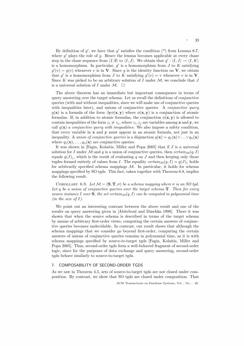
· 33

By definition of g′, we have that g′ satisfies the condition (*) from Lemma 6.7,where g′ plays the role of g. Hence the lemma becomes applicable at every chasestep in the chase sequence from 〈I, ∅〉 to 〈I, J〉. We obtain that g′ : 〈I, J〉 → 〈I,K〉is a homomorphism. In particular, g′ is a homomorphism from J to K satisfyingg′(v) = g(v) whenever v is in V. Since g is the identity function on V, we obtainthat g′ is a homomorphism from J to K satisfying g′(v) = v whenever v is in V.Since K was picked to be an arbitrary solution of I under M, we conclude that Jis a universal solution of I under M.

The above theorem has an immediate but important consequence in terms ofquery answering over the target schema. Let us recall the definitions of conjunctivequeries (with and without inequalities, since we will make use of conjunctive querieswith inequalities later), and unions of conjunctive queries. A conjunctive queryq(x) is a formula of the form ∃yφ(x,y) where φ(x,y) is a conjunction of atomicformulas. If, in addition to atomic formulas, the conjunction φ(x,y) is allowed tocontain inequalities of the form zi 6= zj , where zi, zj are variables among x and y, wecall q(x) a conjunctive query with inequalities. We also impose a safety condition,that every variable in x and y must appear in an atomic formula, not just in aninequality. A union of conjunctive queries is a disjunction q(x) = q1(x)∨ . . .∨qn(x)where q1(x), . . . , qn(x) are conjunctive queries.

It was shown in [Fagin, Kolaitis, Miller and Popa 2005] that if J is a universalsolution for I under M and q is a union of conjunctive queries, then certainM(q, I)equals q(J)↓, which is the result of evaluating q on J and then keeping only thosetuples formed entirely of values from I. The equality certainM(q, I) = q(J)↓ holdsfor arbitrarily specified schema mappings M. In particular, it holds for schemamappings specified by SO tgds. This fact, taken together with Theorem 6.8, impliesthe following result.

Corollary 6.9. Let M = (S,T, σ) be a schema mapping where σ is an SO tgd.Let q be a union of conjunctive queries over the target schema T. Then for everysource instance I over S, the set certainM(q, I) can be computed in polynomial time(in the size of I).

We point out an interesting contrast between the above result and one of theresults on query answering given in [Abiteboul and Duschka 1998]. There it wasshown that when the source schema is described in terms of the target schemaby means of arbitrary first-order views, computing the certain answers of conjunc-tive queries becomes undecidable. In contrast, our result shows that although theschema mappings that we consider go beyond first-order, computing the certainanswers of unions of conjunctive queries remains in polynomial time, as it is withschema mappings specified by source-to-target tgds [Fagin, Kolaitis, Miller andPopa 2005]. Thus, second-order tgds form a well-behaved fragment of second-orderlogic, since for the purposes of data exchange and query answering, second-ordertgds behave similarly to source-to-target tgds.

7. COMPOSABILITY OF SECOND-ORDER TGDS

As we saw in Theorem 4.5, sets of source-to-target tgds are not closed under com-position. By contrast, we show that SO tgds are closed under composition. That


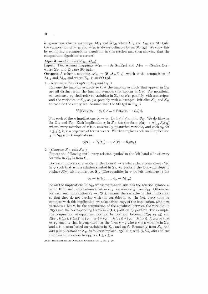
34 ·

is, given two schema mappings M12 and M23 where Σ12 and Σ23 are SO tgds,the composition of M12 and M23 is always definable by an SO tgd. We show thisby exhibiting a composition algorithm in this section and then showing that thecomposition algorithm is correct.

Algorithm Compose(M12, M23)Input: Two schema mappings M12 = (S1,S2,Σ12) and M23 = (S2,S3,Σ23),where Σ12 and Σ23 are SO tgds.Output: A schema mapping M13 = (S1,S3,Σ13), which is the composition ofM12 and M23 and where Σ13 is an SO tgd.1. (Normalize the SO tgds in Σ12 and Σ23.)

Rename the function symbols so that the function symbols that appear in Σ12

are all distinct from the function symbols that appear in Σ23. For notationalconvenience, we shall refer to variables in Σ12 as x’s, possibly with subscripts,and the variables in Σ23 as y’s, possibly with subscripts. Initialize S12 and S23

to each be the empty set. Assume that the SO tgd in Σ12 is

∃f ((∀x1(φ1 → ψ1)) ∧ ... ∧ (∀xn(φn → ψn))).

Put each of the n implications φi → ψi, for 1 ≤ i ≤ n, into S12. We do likewisefor Σ23 and S23. Each implication χ in S12 has the form φ(x) →

∧kj=1Rj(tj)

where every member of x is a universally quantified variable, and each tj, for1 ≤ j ≤ k, is a sequence of terms over x. We then replace each such implicationχ in S12 with k implications:

φ(x) → R1(t1), ..., φ(x) → Rk(tk)

2. (Compose S12 with S23.)Repeat the following until every relation symbol in the left-hand side of everyformula in S23 is from S1.For each implication χ in S23 of the form ψ → γ where there is an atom R(y)in ψ such that R is a relation symbol in S2, we perform the following steps toreplace R(y) with atoms over S1. (The equalities in ψ are left unchanged.) Let

φ1 → R(t1), ..., φp → R(tp)

be all the implications in S12 whose right-hand side has the relation symbol Rin it. If no such implications exist in S12, we remove χ from S23. Otherwise,for each such implication φi → R(ti), rename the variables in this implicationso that they do not overlap with the variables in χ. (In fact, every time wecompose with this implication, we take a fresh copy of the implication, with newvariables.) Let θi be the conjunction of the equalities between the variables inR(y) and the corresponding terms in R(ti), position by position. For example,the conjunction of equalities, position by position, between R(y1, y2, y3) andR(x1, f2(x2), f1(x3)) is (y1 = x1) ∧ (y2 = f2(x2)) ∧ (y3 = f1(x3)). Observe thatevery equality that is generated has the form y = t where y is a variable in Σ23

and t is a term based on variables in Σ12 and on f . Remove χ from S23 andadd p implications to S23 as follows: replace R(y) in χ with φi ∧ θi and add theresulting implication to S23, for 1 ≤ i ≤ p.


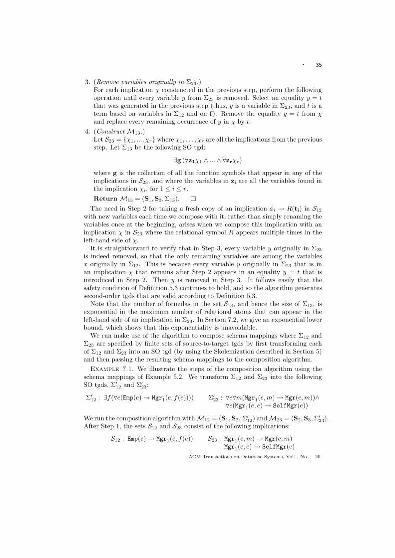
· 35

3. (Remove variables originally in Σ23.)For each implication χ constructed in the previous step, perform the followingoperation until every variable y from Σ23 is removed. Select an equality y = tthat was generated in the previous step (thus, y is a variable in Σ23, and t is aterm based on variables in Σ12 and on f). Remove the equality y = t from χand replace every remaining occurrence of y in χ by t.

4. (Construct M13.)Let S23 = {χ1, ..., χr} where χ1, . . . , χr are all the implications from the previousstep. Let Σ13 be the following SO tgd:

∃g (∀z1χ1 ∧ ... ∧ ∀zrχr)

where g is the collection of all the function symbols that appear in any of theimplications in S23, and where the variables in zi are all the variables found inthe implication χi, for 1 ≤ i ≤ r.Return M13 = (S1,S3,Σ13).

The need in Step 2 for taking a fresh copy of an implication φi → R(ti) in S12

with new variables each time we compose with it, rather than simply renaming thevariables once at the beginning, arises when we compose this implication with animplication χ in S23 where the relational symbol R appears multiple times in theleft-hand side of χ.

It is straightforward to verify that in Step 3, every variable y originally in Σ23

is indeed removed, so that the only remaining variables are among the variablesx originally in Σ12. This is because every variable y originally in Σ23 that is inan implication χ that remains after Step 2 appears in an equality y = t that isintroduced in Step 2. Then y is removed in Step 3. It follows easily that thesafety condition of Definition 5.3 continues to hold, and so the algorithm generatessecond-order tgds that are valid according to Definition 5.3.

Note that the number of formulas in the set S13, and hence the size of Σ13, isexponential in the maximum number of relational atoms that can appear in theleft-hand side of an implication in Σ23. In Section 7.2, we give an exponential lowerbound, which shows that this exponentiality is unavoidable.

We can make use of the algorithm to compose schema mappings where Σ12 andΣ23 are specified by finite sets of source-to-target tgds by first transforming eachof Σ12 and Σ23 into an SO tgd (by using the Skolemization described in Section 5)and then passing the resulting schema mappings to the composition algorithm.

Example 7.1. We illustrate the steps of the composition algorithm using theschema mappings of Example 5.2. We transform Σ12 and Σ23 into the followingSO tgds, Σ′12 and Σ′23:

Σ′12 : ∃f(∀e(Emp(e) → Mgr1(e, f(e)))) Σ′23 : ∀e∀m(Mgr1(e,m) → Mgr(e,m))∧∀e(Mgr1(e, e) → SelfMgr(e))

We run the composition algorithm withM12 = (S1,S2, Σ′12) andM23 = (S2,S3,Σ′23).After Step 1, the sets S12 and S23 consist of the following implications:

S12 : Emp(e) → Mgr1(e, f(e)) S23 : Mgr1(e,m) → Mgr(e,m)Mgr1(e, e) → SelfMgr(e)


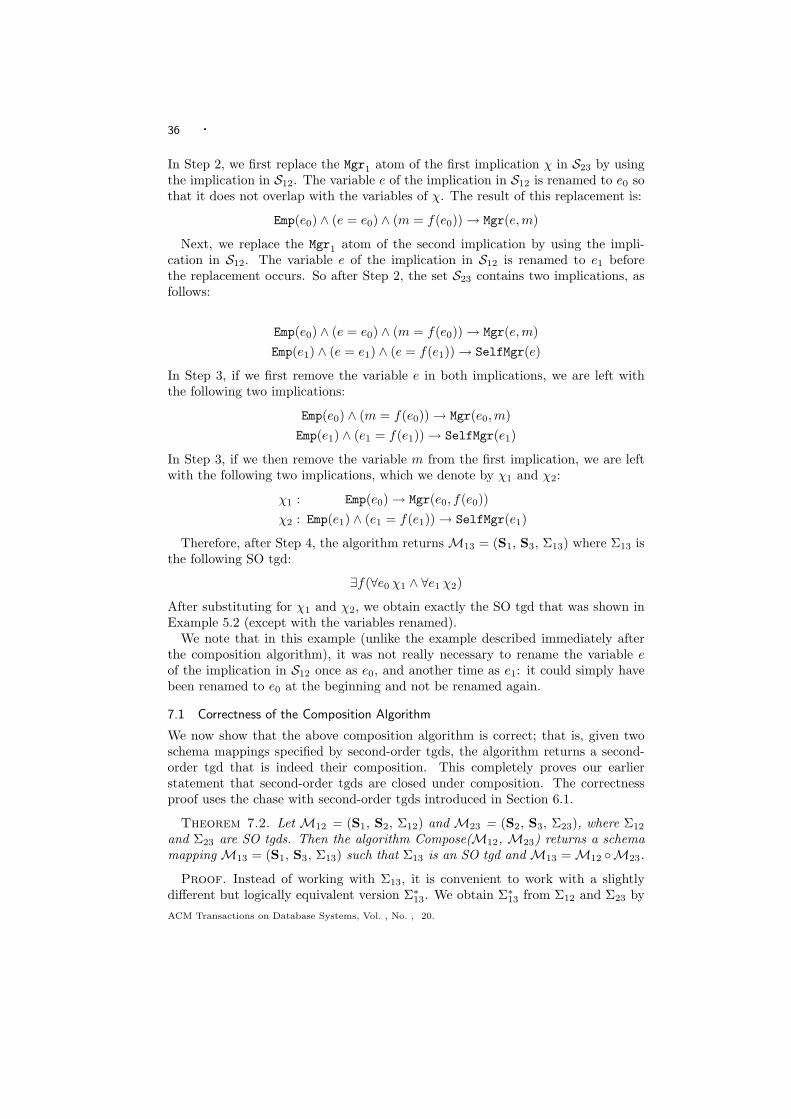
36 ·

In Step 2, we first replace the Mgr1 atom of the first implication χ in S23 by usingthe implication in S12. The variable e of the implication in S12 is renamed to e0 sothat it does not overlap with the variables of χ. The result of this replacement is:

Emp(e0) ∧ (e = e0) ∧ (m = f(e0)) → Mgr(e,m)

Next, we replace the Mgr1 atom of the second implication by using the impli-cation in S12. The variable e of the implication in S12 is renamed to e1 beforethe replacement occurs. So after Step 2, the set S23 contains two implications, asfollows:

Emp(e0) ∧ (e = e0) ∧ (m = f(e0)) → Mgr(e,m)Emp(e1) ∧ (e = e1) ∧ (e = f(e1)) → SelfMgr(e)

In Step 3, if we first remove the variable e in both implications, we are left withthe following two implications:

Emp(e0) ∧ (m = f(e0)) → Mgr(e0,m)Emp(e1) ∧ (e1 = f(e1)) → SelfMgr(e1)

In Step 3, if we then remove the variable m from the first implication, we are leftwith the following two implications, which we denote by χ1 and χ2:

χ1 : Emp(e0) → Mgr(e0, f(e0))χ2 : Emp(e1) ∧ (e1 = f(e1)) → SelfMgr(e1)

Therefore, after Step 4, the algorithm returns M13 = (S1, S3, Σ13) where Σ13 isthe following SO tgd:

∃f(∀e0 χ1 ∧ ∀e1 χ2)

After substituting for χ1 and χ2, we obtain exactly the SO tgd that was shown inExample 5.2 (except with the variables renamed).

We note that in this example (unlike the example described immediately afterthe composition algorithm), it was not really necessary to rename the variable eof the implication in S12 once as e0, and another time as e1: it could simply havebeen renamed to e0 at the beginning and not be renamed again.

7.1 Correctness of the Composition Algorithm

We now show that the above composition algorithm is correct; that is, given twoschema mappings specified by second-order tgds, the algorithm returns a second-order tgd that is indeed their composition. This completely proves our earlierstatement that second-order tgds are closed under composition. The correctnessproof uses the chase with second-order tgds introduced in Section 6.1.

Theorem 7.2. Let M12 = (S1, S2, Σ12) and M23 = (S2, S3, Σ23), where Σ12

and Σ23 are SO tgds. Then the algorithm Compose(M12, M23) returns a schemamapping M13 = (S1, S3, Σ13) such that Σ13 is an SO tgd and M13 = M12 ◦M23.

Proof. Instead of working with Σ13, it is convenient to work with a slightlydifferent but logically equivalent version Σ∗13. We obtain Σ∗13 from Σ12 and Σ23 byACM Transactions on Database Systems, Vol. , No. , 20.

· 37

making two changes to the composition algorithm. The first change is to eliminateStep 3. The second change is to modify Step 4 of the algorithm by letting g bethe collection of all the function symbols that appear in Σ12 or Σ23. Thus, some ofthese existentialized function symbols may not appear in the body (the first-orderpart) of Σ∗13. It is easy to verify that Σ∗13 is logically equivalent to Σ13. Becauseof the elimination of Step 3 of the composition algorithm, Σ∗13 is not necessarily anSO tgd (it may violate the safety condition). However, it is more convenient for usto prove that Σ∗13 defines the composition than to prove directly that Σ13 definesthe composition. Since Σ∗13 is logically equivalent to Σ13, this is sufficient to proveour desired result that Σ13 defines the composition.6

Let T12 be the body of Σ12. So Σ12 is ∃fT12, where f consists of the functionsymbols that appear in Σ12. Similarly, let T23 be the body of Σ23, and let T ∗13 be thebody of Σ∗13. In order to simplify notation, we assume (without loss of generality)that each conjunct in Σ12 is of the form ∀x(φ(x) → R(t)) for a relation symbol R.If Σ12 is not of this form, then as we noted earlier, it can be equivalently rewrittenin this form (and this is essentially what Step 1 in the algorithm does for Σ12).

To show that the schema mapping M13 generated by the algorithm satisfiesM13 = M12 ◦M23, we need to show that for every I1 over schema S1 and for everyI3 over schema S3, we have that 〈I1, I3〉 |= Σ∗13 if and only if there is an I2 overschema S2 such that 〈I1, I2〉 |= Σ12 and 〈I2, I3〉 |= Σ23.

Proof of the “only if” direction. Assume that 〈I1, I3〉 |= Σ∗13, that is,〈U ; I1, I3〉 |= Σ∗13, for a countably infinite universe U that includes the values in I1and I3. We show that there is an I2 such that 〈I1, I2〉 |= Σ12 and 〈I2, I3〉 |= Σ23, forthe same choice U of the universe, that is, 〈U ; I1, I2〉 |= Σ12 and 〈U ; I2, I3〉 |= Σ23.We take Ic

2 such that 〈I1, Ic2〉 is the result of chasing 〈I1, ∅〉 with Σ12. As we re-

marked right after Definition 6.5, we have that 〈I1, Ic2〉 |= Σ12, where the universe

is the set of ground terms over V and f , where V is the set of values in I1.Let g0 be the collection of concrete functions over U such that 〈I1, I3〉 |= T ∗13[g 7→

g0]. By assumption, the function symbols f that appear in Σ12 are all in g. Wedenote by f0 those functions in g0 that replace function symbols in f .

We now take I2 to be the instance that is obtained from Ic2 by instantiating each

ground term u of Ic2 with the concrete value that results when we “evaluate” all

the function terms in u by using the concrete functions f0. It is easy to see thatI2 is an instance whose values are in U . Furthermore, it is easy to verify that〈I1, I2〉 |= T12[f 7→ f0]. In particular, we also have that 〈U ; I1, I2〉 |= Σ12. We willnow show that 〈U ; I2, I3〉 |= Σ23.

Let f ′ be the collection of all the existentially quantified function symbols in Σ23.We can assume without loss of generality that each f ′ in f ′ appears in a conjunct ofΣ23. We show that there are functions f ′0 over U such that 〈I2, I3〉 |= T23[f ′ 7→ f ′0].In particular, this shows that 〈U ; I2, I3〉 |= Σ23. By construction of Σ∗13, each f ′ inf ′ appears among g as some g. We take f ′0 to be g0.

We now show that 〈I2, I3〉 |= T23[f ′ 7→ f ′0]. We need to show that for every

6Although the formula Σ∗13 is not an SO tgd under the definition given in this paper, it is an SO

tgd under the definition given our conference version [Fagin, Kolaitis, Popa and Tan 2004]. This

is the difference, mentioned in Footnote 3, between the definition of SO tgds in this paper and inthe conference version.


38 ·

conjunct ∀y(ψ → γ) in Σ23, we have that 〈I2, I3〉 |= (∀y(ψ → γ))[f ′ 7→ f ′0].Assume that a is a sequence of values of I2 such that I2 |= ψ[f ′ 7→ f ′0,y 7→ a].Moreover, we can assume without loss of generality that ψ is of the form

R1(y1) ∧ . . . ∧Rk(yk) ∧ θ

where the first k literals are the relational atoms of ψ and θ is the conjunction ofthe equalities in ψ. The variables in yp, for each p with 1 ≤ p ≤ k, appear amongthe variables in y. (Also recall that the only terms that appear in such relationalatoms are variables, by the definition of a second-order tgd.)

Since I2 |= ψ[f ′ 7→ f ′0,y 7→ a], it must be the case that I2 contains a tuple ap

in Rp, for each p with 1 ≤ p ≤ k. Here, ap is a sub-tuple of a, consisting of thesequence of values of a that replace the variables in yp. We also have that all theequalities in θ are true when y is replaced by a and f ′ is replaced by f ′0. That is,for each equality t = t′ in θ, we have that t[f ′ 7→ f ′0,y 7→ a] and t′[f ′ 7→ f ′0,y 7→ a]represent the same value.

We know that 〈I1, Ic2〉 is the result of chasing 〈I1, ∅〉 with Σ12, and I2 is the result

of the subsequent “evaluation” of the ground terms in Ic2 by using f0. Thus, it

must be the case that for each tuple ap, with 1 ≤ p ≤ k, there is some conjunct∀xp(φp(xp) → Rp(tp)) in Σ12 such that there is a homomorphism hp from thisconjunct into I1 such that ap is the result of “evaluating” hp(tp) by using f0. Bythe definition of a homomorphism from a conjunct into an instance, it must be thecase that I1 |= φp(hp(xp)), for every p with 1 ≤ p ≤ k. Let h be the union ofh1, . . . , hk. Thus, h acts on the union x of the variables in x1, . . . , xk, and h(x)is defined to be hp(x), whenever x is among xp. (The variables in xi and xj areassumed to be disjoint, for every i and j with 1 ≤ i < j ≤ k.) We obtain that

I1 |= (φ1(x1) ∧ (y1 = t1) ∧ . . . ∧ φk(xk) ∧ (yk = tk)) [x 7→ h(x),y 7→ a, f 7→ f0].

Putting this together with the earlier observation that all the equalities in θ aretrue when y is replaced by a and f ′ is replaced by f ′0, we obtain that

(∗) I1 |= (φ1(x1) ∧ (y1 = t1) ∧ . . . ∧ φk(xk) ∧ (yk = tk) ∧ θ)[x 7→ h(x),y 7→ a, f 7→ f0, f ′ 7→ f ′0].

Since by assumption the function symbols g consist precisely of the function symbolsin f along with those in f ′, condition (*) is equivalent to:

(∗∗) I1 |= (φ1(x1) ∧ (y1 = t1) ∧ . . . ∧ φk(xk) ∧ (yk = tk) ∧ θ)[x 7→ h(x),y 7→ a,g 7→ g0].

By the composition algorithm (Step 2), and by the fact that there is some conjunct∀xp(φp(xp) → Rp(tp)) in Σ12 for each p with 1 ≤ p ≤ k, we are guaranteed thatΣ∗13 contains a conjunct that is obtained from the conjunct ∀y(ψ → γ) in Σ23, byreplacing each of the literals Rp(yp) in ψ with the conjunction φp(xp)∧ (yp = tp).Thus, Σ∗13 contains the following conjunct:

∀x∀y((φ1(x1) ∧ (y1 = t1) ∧ . . . ∧ φk(xk) ∧ (yk = tk) ∧ θ) → γ).

We know by assumption that 〈I1, I3〉 |= T ∗13[g 7→ g0]. Together with condition (**),this last fact implies that I3 |= γ[y 7→ a, f ′ 7→ f ′0]. We used here that the variablesACM Transactions on Database Systems, Vol. , No. , 20.

· 39

in x do not appear in γ; we also used the fact that the function symbols that arein g but not in f ′ do not appear in γ (thus their instantiations do not matter).

Thus, given that I2 |= ψ[f ′ 7→ f ′0,y 7→ a] for some arbitrary tuple a of values, wehave concluded that I3 |= γ[f ′ 7→ f ′0,y 7→ a]. It follows that 〈I2, I3〉 |= (∀y(ψ →γ))[f ′ 7→ f ′0]. This concludes the “only if” direction in the proof.

Proof of the “if” direction. Assume that 〈I1, I2〉 |= Σ12 and 〈I2, I3〉 |= Σ23.By Theorem 5.6, if we take a large enough U that includes the active domains ofI1, I2 and I3, we have that 〈U ; I1, I2〉 |= Σ12 and 〈U ; I2, I3〉 |= Σ23. We will showthat 〈U ; I1, I3〉 |= Σ∗13.

As in the proof of the “only if” direction, let f , f ′ and g denote the collectionsof existentially quantified function symbols in Σ12, Σ23 and Σ∗13, respectively. Weknow that there are concrete functions f and f ′ over U such that 〈I1, I2〉 |= T12[f 7→f0] and 〈I2, I3〉 |= T23[f ′ 7→ f ′0]. By the composition algorithm, each functionsymbol g in g is either (1) a function symbol f that occurs in Σ12 and therefore isin f , or (2) a function symbol f ′ that occurs in Σ23 and therefore is in f ′. In thefirst case, we take g0 to be f0. In the second case, we take g0 to be f ′0. We nowshow that 〈I1, I3〉 |= T13[g 7→ g0].

By the composition algorithm, every conjunct in Σ∗13 has the form C, which wedefine to be

∀x∀y((φ1(x1) ∧ (y1 = t1) ∧ . . . ∧ φk(xk) ∧ (yk = tk) ∧ θ) → γ),

obtained from a conjunct

∀y((R1(y1) ∧ . . . ∧Rk(yk) ∧ θ) → γ)

in Σ23 and k conjuncts

∀x1(φ1(x1) → R1(t1)) . . . ,∀xk(φk(xk) → Rk(tk))

in Σ12. Here, the variables x consist precisely of the variables in x1, . . . ,xk, whilethe variables y consist precisely of the variables in y1, . . . ,yk.

We need to show that 〈I1, I3〉 |= C[g 7→ g0]. Assume that a and b are sequencesof values such that

(i) I1 |= (φ1(x1)∧(y1 = t1)∧. . .∧φk(xk)∧(yk = tk)∧θ) [x 7→ a,y 7→ b,g 7→ g0].

To complete the proof, it suffices to show that I3 |= γ[x 7→ a,y 7→ b,g 7→ g0]. Thisis the same as saying that

(ii) I3 |= γ[y 7→ b, f ′ 7→ f ′0].

Here we made use of the fact that the variables in x do not occur in γ. We alsomade use of the fact that every function symbol g in g that occurs in γ is some f ′

in f ′, and we had earlier picked g0 to be equal to f ′0.We know that 〈I1, I2〉 |= T12[f 7→ f0]. This implies, in particular, that 〈I1, I2〉 |=

∀xp(φp(xp) → Rp(tp))[f 7→ f0], for each p with 1 ≤ p ≤ k. From (i) we derive thatI1 |= φp(xp)[x 7→ a], for each p with 1 ≤ p ≤ k. It follows that I2 |= Rp(tp)[x 7→a, f 7→ f0], for each p with 1 ≤ p ≤ k. At the same time, we can also derive from(i) that yp[y 7→ b] and tp[x 7→ a, f 7→ f0] represent the same tuple of values, foreach p with 1 ≤ p ≤ k. Here we made use of the fact that every function symbol g


40 ·

in g that occurs in tp is some f in f , and we had earlier picked g0 to be equal tof0. We obtain that

I2 |= (R1(y1) ∧ . . . ∧Rk(yk))[y 7→ b].

Furthermore, from (i), we know that for every equality t = t′ in θ, we have thatt[y 7→ b,g 7→ g0] and t′[y 7→ b,g 7→ g0] represent the same value. (Since θ is fromΣ23, the variables in x do not occur in θ and therefore their values do not matter.)We now make use of the fact that every function symbol g in g that occurs in θmust occur in f ′ as some f ′, and that we had earlier picked g0 to be f ′0. We cantherefore infer that all the equalities in θ are satisfied when y is replaced by b andf ′ is replaced by f ′0. We thus obtain the following:

(iii) I2 |= (R1(y1) ∧ . . . ∧Rk(yk) ∧ θ) [y 7→ b, f ′ 7→ f ′0].

We know that 〈I2, I3〉 |= T23[f ′ 7→ f ′0]. This implies, in particular, that 〈I2, I3〉 |=∀y(R1(y1) ∧ . . . ∧ Rk(yk) ∧ θ → γ)[f ′ 7→ f ′0]. Together with (iii), this implies theearlier statement (ii). This concludes the “if” direction in the proof.

7.2 The Size of the Composition Formula

Assume that M13 = M12 ◦M23 where M13 = (S1,S3,Σ13). We may refer to Σ13

as the composition formula. When we defined our composition algorithm, we notedthat the size of the composition formula that we constructed might be exponential.We now prove an exponential lower bound, which shows that this exponentiality isunavoidable.

Proposition 7.3. There are schema mappings M12 = (S1, S2, Σ12) and M23 =(S2,S3,Σ23), where Σ12 and Σ23 are finite sets of full source-to-target tgds, suchthat if M12 ◦M23 = (S1, S3, Σ13), then every set Σ′13 of source-to-target tgds thatis logically equivalent to Σ13, and every SO tgd Σ′13 that is logically equivalent toΣ13, is of size exponential in the size of Σ12 ∪ Σ23.

Proof. Let S1 consist of the unary relation symbols R1, . . . , Rn and R′1, . . . R′n.

Let S2 consist of the unary relation symbols S1, . . . , Sn, and let S3 consist of theunary relation symbol T . Let Σ12 consist of the full source-to-target tgds Ri(x) →Si(x), for 1 ≤ i ≤ n, and the full source-to-target tgds R′i(x) → Si(x), for 1 ≤ i ≤ n.Let Σ23 consist of the single full source-to-target tgd S1(x)∧· · ·∧Sn(x) → T (x). LetΣ13 consist of all of the source-to-target tgds of the form U1(x)∧· · ·∧Un(x) → T (x),where Ui is either Ri or R′i, for 1 ≤ i ≤ n. It is straightforward to verify thatM12 ◦ M23 = (S1, S3, Σ13). Let Σ′13 be a set of source-to-target tgds that islogically equivalent to Σ13. We shall show that Σ′13 contains at least 2n members.A similar proof show that if Σ′13 is an SO tgd, then it contains at least 2n conjuncts.This is sufficient to prove the theorem.

We first show that the left-hand side of every member of Σ′13 must contain atleast one of Ri or R′i, for each i. Assume not; we shall derive a contradiction. Letτ be a member of Σ′13 such that there is i for which τ does not contain Ri and τdoes not contain R′i. Let I be a source instance (an S1 instance) that consists ofthe facts Rj(0) and R′j(0) for each j 6= i, but where the Ri and R′i relations areempty. Let J be a target instance (an S3 instance) where the T relation is empty.It is clear that 〈I, J〉 satisfies Σ13, since every member of Σ13 contains either Ri


· 41

or R′i in its left-hand side. However, 〈I, J〉 does not satisfy τ , since when everyvariable appearing in the left-hand side of τ takes on the value 0, the left-handside of τ is satisfied but the right-hand side of τ is not (since the T relation of Jis empty). Since 〈I, J〉 satisfies Σ13 but does not satisfy Σ′13, this contradicts theassumption that Σ′13 is logically equivalent to Σ13. So indeed, the left-hand side ofevery member of Σ′13 must contain at least one of Ri or R′i, for each i.

We now show that for each of the 2n vectors x = (x1, . . . , xn) where each xi iseither 0 or 1, there is a member σx of Σ′13 such that for each i, the left-hand sideof σx contains Ri precisely if xi = 0, and the left-hand side contains R′i preciselyif xi = 1. Assume not; we shall derive a contradiction. Let y = (y1, . . . , yn) be aspecific 0,1 vector where this condition is violated, that is, where Σ′13 has no suchmember σy. Let I be a source instance that contains exactly n facts, namely, foreach i, the fact Ri(0) when yi = 0 or the fact R′i(0) when yi = 1, Let J be atarget instance where the T relation is empty. We now show that 〈I, J〉 satisfiesevery member of Σ′13. Let τ be an arbitrary member of Σ′13. From what we showedearlier, we know that the left-hand side of τ must contain at least one of Ri orR′i, for each i. Since also τ is not of the form σy, it follows that either there is isuch that yi = 0 and τ contains R′i, or yi = 1 and τ contains Ri. Therefore 〈I, J〉satisfies τ , since the left-hand side of τ is never satisfied in I, no matter what thechoice is of the variables in the left-hand side of τ . Since τ is an arbitrary memberof Σ′13, it follows that 〈I, J〉 satisfies Σ′13. Now Σ13 has a member γ of the form σy.It is easy to see that 〈I, J〉 does not satisfy γ, and so 〈I, J〉 does not satisfy Σ13.Since 〈I, J〉 satisfies Σ′13 but does not satisfy Σ13, this contradicts the assumptionthat Σ′13 is logically equivalent to Σ13.

Since Σ′13 contains a member σx for each of the 2n vectors x = (x1, . . . , xn) whereeach xi is either 0 or 1, and since it is clear that each such member σx is distinct,it follows that Σ′13 contains at least 2n members. This was to be shown.

7.3 Failure of the Active Domain Semantics

In our definition of the semantics of SO tgds, we took the universe (which serves asthe domain and range of the existentially quantified functions) to be a countablyinfinite set that includes the active domain. (We later showed that a finite but largeenough universe that includes the active domain also suffices.) In this section, weshow that if we were to instead take the universe to be simply the active domain,then an SO tgd that results after applying the composition algorithm might havea meaning that is different from that of composition. We also include a discussionon domain independence of SO tgds. Let us refer to our usual semantics as the“infinite universe semantics”, and let us refer to the semantics where the universeis taken to be the active domain as the “active domain semantics”.

Example 7.4. We consider a slight variation of Example 5.2, with the followingschemas S1, S2 and S3. Schema S1 consists of a single unary relation symbol Emp ofemployees. Schema S2 consists of a single binary relation symbol Mgr, associatingeach employee with a manager. Schema S3 consists of a single unary relation symbolSelfMgr, intended to store employees who are their own manager. Consider theschema mappings M12 = (S1, S2,Σ12) and M23 = (S2,S3,Σ23), where

Σ12 = { ∀e (Emp(e) → ∃mMgr(e,m)) } Σ23 = { ∀e(Mgr(e, e) → SelfMgr(e)) }.ACM Transactions on Database Systems, Vol. , No. , 20.

42 ·

It is easy to verify that the composition algorithm tells us that the composition ofM12 and M23 is M13 = (S1, S3,Σ13), where Σ13 is the following second-order tgd:

∃f(∀e(Emp(e) ∧ (e = f(e)) → SelfMgr(e))). (4)

In the infinite universe semantics, this formula (4) is equivalent to “Truth”, thatis, formula (4) is a tautology that holds for every choice of 〈I1, I3〉. This is becausewe can simply select an arbitrary function f such that f(e) 6= e for every e in thedomain. Then the left-hand side Emp(e) ∧ (e = f(e)) is false for every e, and so∀e(Emp(e) ∧ (e = f(e)) → SelfMgr(e)) holds for this f . And indeed, “Truth” isthe right answer for the composition of M12 and M23, as we now show. Let I1 bean arbitrary instance of schema S1 and let I3 be an arbitrary instance of schemaS3. To show that the composition is indeed “Truth”, we must show that 〈I1, I3〉is in the composition. Define the instance I2 of schema S2 by letting Bob be someelement different from every member of EmpI1 , and letting MgrI2 contain all tuples(e,Bob), where e is in EmpI1 . Then 〈I1, I2〉 |= Σ12 and 〈I2, I3〉 |= Σ23, and so 〈I1, I3〉is in the composition, as desired.

We now show that in the active domain semantics, the formula (4) is not equiv-alent to “Truth”. Therefore, the formula (4) given by the composition algorithm,does not have the right meaning, of composition, under the active domain seman-tics. We need only show that there is an instance I1 of schema S1 and an instance I3of schema S3 such that 〈I1, I3〉 does not satisfy (4) in the active domain semantics.

Define I1 by letting EmpI1 contain the single element Alice. Define I3 by lettingSelfMgrI3 be empty. The active domain is {Alice}, and there is only one functionwith domain and range {Alice}, namely the function f0 where f0(Alice) = Alice.Using this function f0 (the only function available) for f , the left-hand side Emp(e)∧(e = f(e)) is satisfied when e is Alice, but the right-hand side SelfMgr(e) is not.So 〈I1, I3〉 does not satisfy the formula (4) in the active domain semantics, whichwas to be shown.

A formula is said to be domain independent if its truth does not depend on thechoice of universe, as long as the universe contains the active domain. Fagin [Fagin1982] was the first to observe that the safety condition for first-order dependencies(that every universally quantified variable must appear in the left-hand side) makesthem domain independent. This comment applies to the (first-order) source-to-target tgds we consider. However, it follows from Example 7.4 that SO tgds arenot domain independent. Thus, in this example, let U ′ = {Alice}, which is theactive domain, and let U = {Alice,Bob}. It follows easily from the discussion inExample 7.4 that 〈U ; I, J〉 |= Σ13 but 〈U ′; I, J〉 6|= Σ13. Therefore, the SO tgd Σ13

is not domain independent.7 On the other hand, our earlier Theorem 5.6 impliesthat SO tgds obey a limited form of domain independence: the choice of universedoes not matter, as long as it contains the active domain and is sufficiently large.

8. SO TGDS ARE EXACTLY THE NEEDED CLASS

We have introduced SO tgds since (1) every finite set of (first-order) source-to-target tgds is logically equivalent to an SO tgd and (2) SO tgds are closed under

7Sergey Melnik pointed out to us that SO tgds are not necessarily domain independent, usingessentially this example.


· 43

composition. We therefore obtain the following theorem.

Theorem 8.1. The composition of a finite number of schema mappings, eachdefined by a finite set of source-to-target tgds, is defined by an SO tgd.

In this section, we prove a converse to Theorem 8.1. Specifically, we prove thefollowing theorem.

Theorem 8.2. Every SO tgd defines the composition of a finite number of schemamappings, each defined by a finite set of source-to-target tgds.

We note that in Theorem 8.2, the “intermediate” schemas depend on the SOtgd. We now show that Theorem 8.2 gives us the next theorem. This next theoremshows the naturalness and “inevitability” of the class of SO tgds.

Theorem 8.3. SO tgds form the smallest class (up to logical equivalence) thatcontains every source-to-target tgd and is closed under conjunction and composition.

Proof. We already noted that every source-to-target tgd is logically equivalentto an SO tgd, and that the conjunction of a pair of SO tgds is logically equivalentto an SO tgd. Also, Theorem 7.2 tells us that the composition of two schemamappings, each defined by an SO tgd, is defined by an SO tgd. These facts tell usthat, up to logical equivalence, the class of SO tgds contains every source-to-targettgd and is closed under conjunction and composition.

We now show that the class of SO tgds is (up to logical equivalence) the smallestsuch class. Let Y be a class that contains every source-to-target tgd and is closedunder conjunction and composition. We must show that for each SO tgd σ there isa member of Y that is logically equivalent to σ. By Theorem 8.2, there are finitesets Σ12, ..., Σn(n+1) of source-to-target tgds such that σ defines the compositionof the mappings given by Σ12, ..., Σn(n+1). For each i, with 1 ≤ i ≤ n, sinceΣi(i+1) is a finite set of source-to-target tgds, and since Y contains each member ofΣi(i+1) and is closed under conjunction, it follows that Y contains the conjunctionof the members of Σi(i+1). Since Y is closed under composition, Y contains thecomposition formula of the schema mappings defined by Σ12, ..., Σn(n+1). But thiscomposition formula is logically equivalent to σ. So there is a member of Y that islogically equivalent to σ. This was to be shown.

It remains to prove Theorem 8.2. We shall prove Theorem 8.2 by proving aslightly stronger theorem. Before we state this stronger theorem, we need a defini-tion. The depth of a term is as defined in Section 5.2. We define the nesting depthof an SO tgd σ to be the largest depth of the terms that appear in σ. For example,let σ be the SO tgd

∃f∃g(S(x, y) → T (x, f(y), g(x, f(y))).

Then σ has nesting depth 2, since the term with the largest depth that appears inσ is g(x, f(y)), which has depth 2.

We shall prove the following theorem, which immediately implies Theorem 8.2.

Theorem 8.4. Every SO tgd of nesting depth r defines the composition of r+1schema mappings, each defined by a finite set of source-to-target tgds.


44 ·

Proof. It is instructive to first prove this theorem for some special cases, to getthe idea of the construction. Let σ′ be the formula ∀x(S(x) → T (f(x), g(x), f(g(x))),and let σ be the SO tgd ∃f∃gσ′. Thus, σ is

∃f∃g∀x(S(x) → T (f(x), g(x), f(g(x))).

Define Σ12 to consist of the following source-to-target tgds:

∀x(S(x) → S1(x))∀x(S(x) → ∃yF1(x, y))∀x(S(x) → ∃yG1(x, y)).

Intuitively, we take S1 to copy S, we take F1(x, y) to encode f(x) = y, and we takeG1(x, y) to encode g(x) = y. The second dependency has the effect of guaranteeingthat f(x) is defined whenever S(x) holds, and the third dependency has the effectof guaranteeing that g(x) is defined whenever S(x) holds.

Define Σ23 to consist of the following source-to-target tgds:

∀x(S1(x) → S2(x))∀x∀y(F1(x, y) → F2(x, y))∀x∀y(G1(x, y) → G2(x, y))∀x∀y(G1(x, y) → ∃zF2(y, z)).

Intuitively, we take S2 to copy S1, F2 to copy F1, and G2 to copy G1. The fourthdependency has the effect of guaranteeing that f(y) is defined for all y in the rangeof g.

Define Σ34 to consist of the following source-to-target tgd:

∀x∀y∀y′∀z((S2(x) ∧ F2(x, y) ∧G2(x, y′) ∧ F2(y′, z)) → T (y, y′, z)). (5)

Intuitively, formula (5) says

∀x∀y∀y′∀z((S(x) ∧ (f(x) = y) ∧ (g(x) = y′) ∧ (f(y′) = z) → T (y, y′, z)). (6)

In turn, formula (6) says

∀x(S(x) → T (f(x), g(x), f(g(x))). (7)

Note that formula (7) is exactly the “body” of σ.We now show that 〈I1, I4〉 |= σ if and only if there are I2, I3 such that 〈I1, I2〉 |=

Σ12, 〈I2, I3〉 |= Σ23, and 〈I3, I4〉 |= Σ34. This is sufficient to prove the theoremin this special case. Assume first that 〈I1, I4〉 |= σ. So there are f0, g0 such that〈I1, I4〉 |= σ′[f 7→ f0, g 7→ g0]. We see from Theorem 5.6 that we can assumewithout loss of generality that the universe is finite. Define I2 by taking S1 toequal S, taking F1(a, b) to hold in I2 precisely if f0(a) = b, and taking G1(a, b)to hold in I2 precisely if g0(a) = b. Define I3 by taking S2 to equal S, taking F2

to equal F1, and taking G2 to equal G1. Note that I2 and I3 are finite, becauseof our assumption that the universe is finite. It is straightforward to verify that〈I1, I2〉 |= Σ12, 〈I2, I3〉 |= Σ23, and 〈I3, I4〉 |= Σ34.

Assume now that 〈I1, I2〉 |= Σ12, 〈I2, I3〉 |= Σ23, and 〈I3, I4〉 |= Σ34. Let U (theuniverse) be a countably infinite set that contains all values that appear in any ofI1, I2, I3, or I4. Define f0(a) for a in U as follows. If there is some b such thatACM Transactions on Database Systems, Vol. , No. , 20.

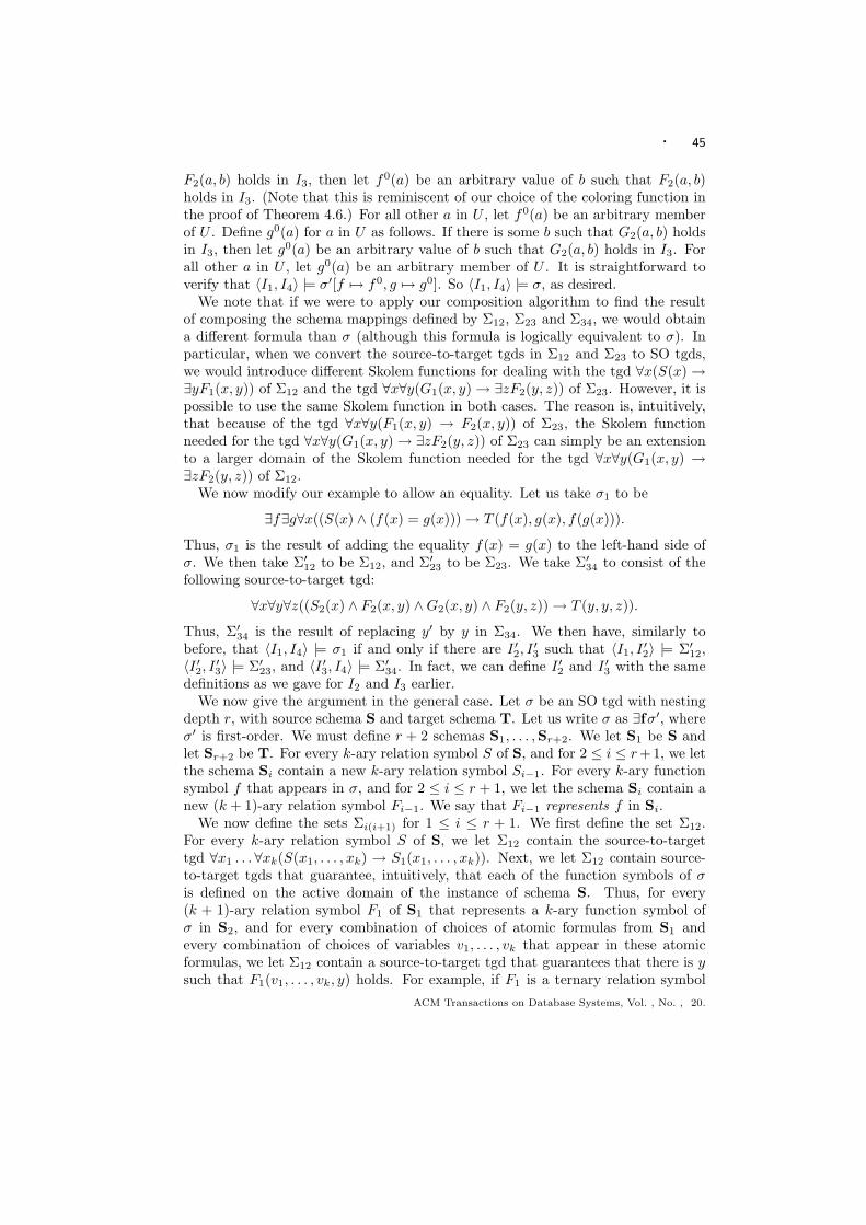
· 45

F2(a, b) holds in I3, then let f0(a) be an arbitrary value of b such that F2(a, b)holds in I3. (Note that this is reminiscent of our choice of the coloring function inthe proof of Theorem 4.6.) For all other a in U , let f0(a) be an arbitrary memberof U . Define g0(a) for a in U as follows. If there is some b such that G2(a, b) holdsin I3, then let g0(a) be an arbitrary value of b such that G2(a, b) holds in I3. Forall other a in U , let g0(a) be an arbitrary member of U . It is straightforward toverify that 〈I1, I4〉 |= σ′[f 7→ f0, g 7→ g0]. So 〈I1, I4〉 |= σ, as desired.

We note that if we were to apply our composition algorithm to find the resultof composing the schema mappings defined by Σ12, Σ23 and Σ34, we would obtaina different formula than σ (although this formula is logically equivalent to σ). Inparticular, when we convert the source-to-target tgds in Σ12 and Σ23 to SO tgds,we would introduce different Skolem functions for dealing with the tgd ∀x(S(x) →∃yF1(x, y)) of Σ12 and the tgd ∀x∀y(G1(x, y) → ∃zF2(y, z)) of Σ23. However, it ispossible to use the same Skolem function in both cases. The reason is, intuitively,that because of the tgd ∀x∀y(F1(x, y) → F2(x, y)) of Σ23, the Skolem functionneeded for the tgd ∀x∀y(G1(x, y) → ∃zF2(y, z)) of Σ23 can simply be an extensionto a larger domain of the Skolem function needed for the tgd ∀x∀y(G1(x, y) →∃zF2(y, z)) of Σ12.

We now modify our example to allow an equality. Let us take σ1 to be

∃f∃g∀x((S(x) ∧ (f(x) = g(x))) → T (f(x), g(x), f(g(x))).

Thus, σ1 is the result of adding the equality f(x) = g(x) to the left-hand side ofσ. We then take Σ′12 to be Σ12, and Σ′23 to be Σ23. We take Σ′34 to consist of thefollowing source-to-target tgd:

∀x∀y∀z((S2(x) ∧ F2(x, y) ∧G2(x, y) ∧ F2(y, z)) → T (y, y, z)).

Thus, Σ′34 is the result of replacing y′ by y in Σ34. We then have, similarly tobefore, that 〈I1, I4〉 |= σ1 if and only if there are I ′2, I

′3 such that 〈I1, I ′2〉 |= Σ′12,

〈I ′2, I ′3〉 |= Σ′23, and 〈I ′3, I4〉 |= Σ′34. In fact, we can define I ′2 and I ′3 with the samedefinitions as we gave for I2 and I3 earlier.

We now give the argument in the general case. Let σ be an SO tgd with nestingdepth r, with source schema S and target schema T. Let us write σ as ∃fσ′, whereσ′ is first-order. We must define r + 2 schemas S1, . . . ,Sr+2. We let S1 be S andlet Sr+2 be T. For every k-ary relation symbol S of S, and for 2 ≤ i ≤ r+1, we letthe schema Si contain a new k-ary relation symbol Si−1. For every k-ary functionsymbol f that appears in σ, and for 2 ≤ i ≤ r + 1, we let the schema Si contain anew (k + 1)-ary relation symbol Fi−1. We say that Fi−1 represents f in Si.

We now define the sets Σi(i+1) for 1 ≤ i ≤ r + 1. We first define the set Σ12.For every k-ary relation symbol S of S, we let Σ12 contain the source-to-targettgd ∀x1 . . .∀xk(S(x1, . . . , xk) → S1(x1, . . . , xk)). Next, we let Σ12 contain source-to-target tgds that guarantee, intuitively, that each of the function symbols of σis defined on the active domain of the instance of schema S. Thus, for every(k + 1)-ary relation symbol F1 of S1 that represents a k-ary function symbol ofσ in S2, and for every combination of choices of atomic formulas from S1 andevery combination of choices of variables v1, . . . , vk that appear in these atomicformulas, we let Σ12 contain a source-to-target tgd that guarantees that there is ysuch that F1(v1, . . . , vk, y) holds. For example, if F1 is a ternary relation symbol


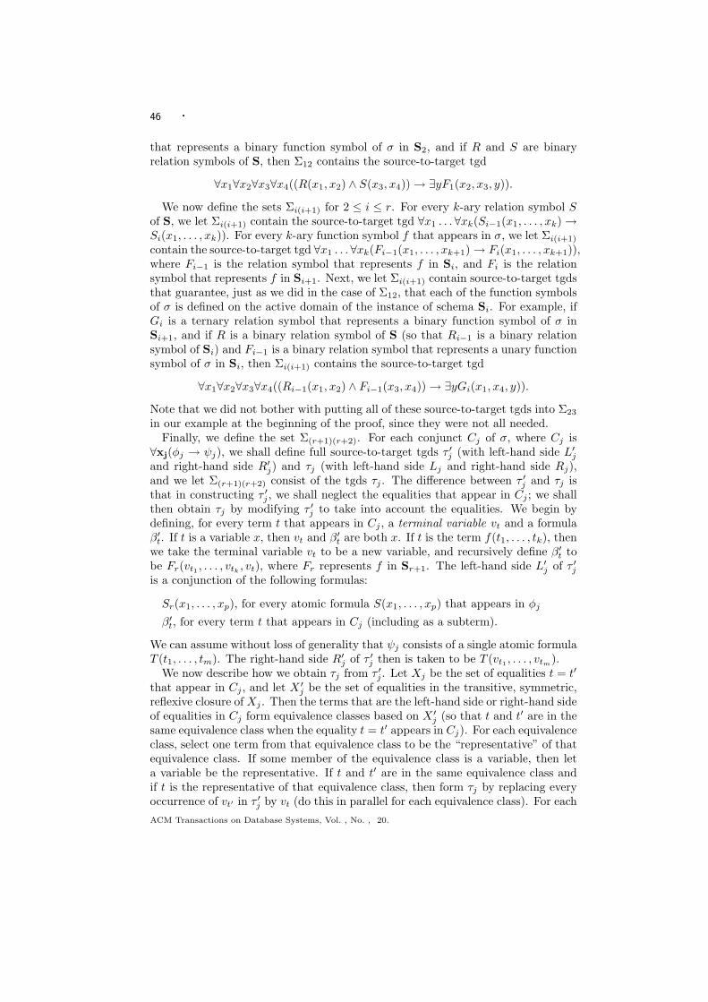
46 ·

that represents a binary function symbol of σ in S2, and if R and S are binaryrelation symbols of S, then Σ12 contains the source-to-target tgd

∀x1∀x2∀x3∀x4((R(x1, x2) ∧ S(x3, x4)) → ∃yF1(x2, x3, y)).

We now define the sets Σi(i+1) for 2 ≤ i ≤ r. For every k-ary relation symbol Sof S, we let Σi(i+1) contain the source-to-target tgd ∀x1 . . .∀xk(Si−1(x1, . . . , xk) →Si(x1, . . . , xk)). For every k-ary function symbol f that appears in σ, we let Σi(i+1)

contain the source-to-target tgd ∀x1 . . .∀xk(Fi−1(x1, . . . , xk+1) → Fi(x1, . . . , xk+1)),where Fi−1 is the relation symbol that represents f in Si, and Fi is the relationsymbol that represents f in Si+1. Next, we let Σi(i+1) contain source-to-target tgdsthat guarantee, just as we did in the case of Σ12, that each of the function symbolsof σ is defined on the active domain of the instance of schema Si. For example, ifGi is a ternary relation symbol that represents a binary function symbol of σ inSi+1, and if R is a binary relation symbol of S (so that Ri−1 is a binary relationsymbol of Si) and Fi−1 is a binary relation symbol that represents a unary functionsymbol of σ in Si, then Σi(i+1) contains the source-to-target tgd

∀x1∀x2∀x3∀x4((Ri−1(x1, x2) ∧ Fi−1(x3, x4)) → ∃yGi(x1, x4, y)).

Note that we did not bother with putting all of these source-to-target tgds into Σ23

in our example at the beginning of the proof, since they were not all needed.Finally, we define the set Σ(r+1)(r+2). For each conjunct Cj of σ, where Cj is

∀xj(φj → ψj), we shall define full source-to-target tgds τ ′j (with left-hand side L′jand right-hand side R′j) and τj (with left-hand side Lj and right-hand side Rj),and we let Σ(r+1)(r+2) consist of the tgds τj . The difference between τ ′j and τj isthat in constructing τ ′j , we shall neglect the equalities that appear in Cj ; we shallthen obtain τj by modifying τ ′j to take into account the equalities. We begin bydefining, for every term t that appears in Cj , a terminal variable vt and a formulaβ′t. If t is a variable x, then vt and β′t are both x. If t is the term f(t1, . . . , tk), thenwe take the terminal variable vt to be a new variable, and recursively define β′t tobe Fr(vt1 , . . . , vtk

, vt), where Fr represents f in Sr+1. The left-hand side L′j of τ ′jis a conjunction of the following formulas:

Sr(x1, . . . , xp), for every atomic formula S(x1, . . . , xp) that appears in φj

β′t, for every term t that appears in Cj (including as a subterm).

We can assume without loss of generality that ψj consists of a single atomic formulaT (t1, . . . , tm). The right-hand side R′j of τ ′j then is taken to be T (vt1 , . . . , vtm

).We now describe how we obtain τj from τ ′j . Let Xj be the set of equalities t = t′

that appear in Cj , and let X ′j be the set of equalities in the transitive, symmetric,

reflexive closure of Xj . Then the terms that are the left-hand side or right-hand sideof equalities in Cj form equivalence classes based on X ′

j (so that t and t′ are in thesame equivalence class when the equality t = t′ appears in Cj). For each equivalenceclass, select one term from that equivalence class to be the “representative” of thatequivalence class. If some member of the equivalence class is a variable, then leta variable be the representative. If t and t′ are in the same equivalence class andif t is the representative of that equivalence class, then form τj by replacing everyoccurrence of vt′ in τ ′j by vt (do this in parallel for each equivalence class). For eachACM Transactions on Database Systems, Vol. , No. , 20.

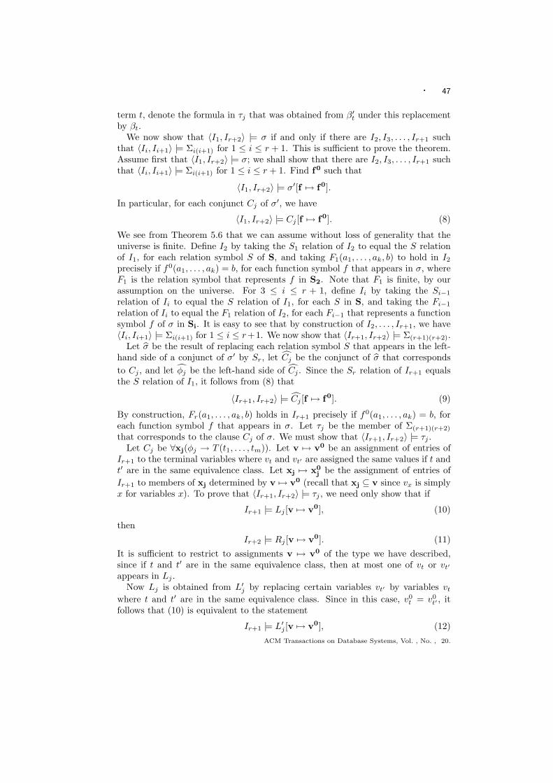
· 47

term t, denote the formula in τj that was obtained from β′t under this replacementby βt.

We now show that 〈I1, Ir+2〉 |= σ if and only if there are I2, I3, . . . , Ir+1 suchthat 〈Ii, Ii+1〉 |= Σi(i+1) for 1 ≤ i ≤ r + 1. This is sufficient to prove the theorem.Assume first that 〈I1, Ir+2〉 |= σ; we shall show that there are I2, I3, . . . , Ir+1 suchthat 〈Ii, Ii+1〉 |= Σi(i+1) for 1 ≤ i ≤ r + 1. Find f0 such that

〈I1, Ir+2〉 |= σ′[f 7→ f0].

In particular, for each conjunct Cj of σ′, we have

〈I1, Ir+2〉 |= Cj [f 7→ f0]. (8)

We see from Theorem 5.6 that we can assume without loss of generality that theuniverse is finite. Define I2 by taking the S1 relation of I2 to equal the S relationof I1, for each relation symbol S of S, and taking F1(a1, . . . , ak, b) to hold in I2precisely if f0(a1, . . . , ak) = b, for each function symbol f that appears in σ, whereF1 is the relation symbol that represents f in S2. Note that F1 is finite, by ourassumption on the universe. For 3 ≤ i ≤ r + 1, define Ii by taking the Si−1

relation of Ii to equal the S relation of I1, for each S in S, and taking the Fi−1

relation of Ii to equal the F1 relation of I2, for each Fi−1 that represents a functionsymbol f of σ in Si. It is easy to see that by construction of I2, . . . , Ir+1, we have〈Ii, Ii+1〉 |= Σi(i+1) for 1 ≤ i ≤ r+1. We now show that 〈Ir+1, Ir+2〉 |= Σ(r+1)(r+2).

Let σ be the result of replacing each relation symbol S that appears in the left-hand side of a conjunct of σ′ by Sr, let Cj be the conjunct of σ that correspondsto Cj , and let φj be the left-hand side of Cj . Since the Sr relation of Ir+1 equalsthe S relation of I1, it follows from (8) that

〈Ir+1, Ir+2〉 |= Cj [f 7→ f0]. (9)

By construction, Fr(a1, . . . , ak, b) holds in Ir+1 precisely if f0(a1, . . . , ak) = b, foreach function symbol f that appears in σ. Let τj be the member of Σ(r+1)(r+2)

that corresponds to the clause Cj of σ. We must show that 〈Ir+1, Ir+2〉 |= τj .Let Cj be ∀xj(φj → T (t1, . . . , tm)). Let v 7→ v0 be an assignment of entries of

Ir+1 to the terminal variables where vt and vt′ are assigned the same values if t andt′ are in the same equivalence class. Let xj 7→ x0

j be the assignment of entries ofIr+1 to members of xj determined by v 7→ v0 (recall that xj ⊆ v since vx is simplyx for variables x). To prove that 〈Ir+1, Ir+2〉 |= τj , we need only show that if

Ir+1 |= Lj [v 7→ v0], (10)

then

Ir+2 |= Rj [v 7→ v0]. (11)

It is sufficient to restrict to assignments v 7→ v0 of the type we have described,since if t and t′ are in the same equivalence class, then at most one of vt or vt′

appears in Lj .Now Lj is obtained from L′j by replacing certain variables vt′ by variables vt

where t and t′ are in the same equivalence class. Since in this case, v0t = v0

t′ , itfollows that (10) is equivalent to the statement

Ir+1 |= L′j [v 7→ v0], (12)ACM Transactions on Database Systems, Vol. , No. , 20.

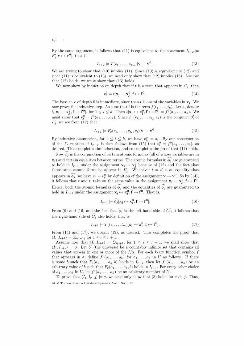
48 ·

By the same argument, it follows that (11) is equivalent to the statement Ir+2 |=R′j [v 7→ v0], that is,

Ir+2 |= T (vt1 , . . . , vtm)[v 7→ v0]. (13)

We are trying to show that (10) implies (11). Since (10) is equivalent to (12) andsince (11) is equivalent to (13), we need only show that (12) implies (13). Assumethat (12) holds; we must show that (13) holds.

We now show by induction on depth that if t is a term that appears in Cj , then

v0t = t[xj 7→ x0

j , f 7→ f0]. (14)

The base case of depth 0 is immediate, since then t is one of the variables in xj. Wenow prove the inductive step. Assume that t is the term f(t1, . . . , tk). Let ai denoteti[xj 7→ x0

j , f 7→ f0], for 1 ≤ i ≤ k. Then t[xj 7→ x0j , f 7→ f0] = f0(a1, . . . , ak). We

must show that v0t = f0(a1, . . . , ak). Since Fr(vt1 , . . . , vtk

, vt) is the conjunct β′t ofL′j , we see from (12) that

Ir+1 |= Fr(vt1 , . . . , vtk, vt)[v 7→ v0]. (15)

By inductive assumption, for 1 ≤ i ≤ k, we have v0ti

= ai. By our constructionof the Fr relation of Ir+1, it then follows from (15) that v0

t = f0(a1, . . . , ak), asdesired. This completes the induction, and so completes the proof that (14) holds.

Now φj is the conjunction of certain atomic formulas (all of whose variables are inxj) and certain equalities between terms. The atomic formulas in φj are guaranteedto hold in Ir+1 under the assignment xj 7→ x0

j because of (12) and the fact thatthese same atomic formulas appear in L′j . Whenever t = t′ is an equality thatappears in φj , we have v0

t = v0t′ by definition of the assignment v 7→ v0. So by (14),

it follows that t and t′ take on the same value in the assignment xj 7→ x0j , f 7→ f0.

Hence, both the atomic formulas of φj and the equalities of φj are guaranteed tohold in Ir+1 under the assignment xj 7→ x0

j , f 7→ f0. That is,

Ir+1 |= φj [xj 7→ x0j , f 7→ f0]. (16)

From (9) and (16) and the fact that φj is the left-hand side of Cj , it follows thatthe right-hand side of Cj also holds, that is,

Ir+2 |= T (t1, . . . , tm)[xj 7→ x0j , f 7→ f0]. (17)

From (14) and (17), we obtain (13), as desired. This completes the proof that〈Ii, Ii+1〉 |= Σi(i+1) for 1 ≤ i ≤ r + 1.

Assume now that 〈Ii, Ii+1〉 |= Σi(i+1) for 1 ≤ i ≤ r + 1; we shall show that〈I1, Ir+2〉 |= σ. Let U (the universe) be a countably infinite set that contains allvalues that appear in one or more of the Ii’s. For each k-ary function symbol fthat appears in σ, define f0(a1, . . . , ak) for a1, . . . , ak in U as follows. If thereis some b such that Fr(a1, . . . , ak, b) holds in Ir+1, then let f0(a1, . . . , ak) be anarbitrary value of b such that Fr(a1, . . . , ak, b) holds in Ir+1. For every other choiceof a1, . . . , ak in U , let f0(a1, . . . , ak) be an arbitrary member of U .

To prove that 〈I1, Ir+2〉 |= σ, we need only show that (8) holds for each j. Thus,ACM Transactions on Database Systems, Vol. , No. , 20.

· 49

assume

I1 |= φj [xj 7→ x0j , f 7→ f0]; (18)

we must show that (17) holds. Since φj is the result of replacing each relationsymbol S of φj by Sr, and since the Sr relation of Ir+1 equals the S relation of I1,it follows from (18) that (16) holds.

For simplicity of notation, let us denote t[xj 7→ x0j , f 7→ f0] by t0. We now show,

by induction on s with 1 ≤ s ≤ r, that Σ12, . . . ,Σs(s+1) assure that if t is a termf(t1, . . . , tk) of depth s, then Fs(t01, . . . , t

0k, t

0) holds in Is+1 (and in particular t0

appears in Is+1).Let us consider first the base case s = 1. In this case, t01, . . . , t

0k are each

members of the active domain of I1, and Σ12 guarantees that there is b suchthat F1(t01, . . . , t

0k, b) holds in I2. By our construction of f0, it then follows that

F1(t01, . . . , t0k, t

0) holds in I2.The inductive step is similar. Let t be the term f(t1, . . . , tk) of depth s + 1,

where s < r. Then t1, . . . , tk each have depth at most s, and so by inductivehypothesis, Σ12, . . . ,Σs(s+1) assure that t01, . . . , t

0k appear in Is+1. Then Σ(s+1)(s+2)

guarantees additionally that there is b such that Fs+1(t01, . . . , t0k, b) holds in Is+2.

By our construction of f0, it then follows that Fs+1(t01, . . . , t0k, t

0) holds in Is+2.This completes the induction. Therefore, Σ12, . . . ,Σr(r+1) assure that if t is a termf(t1, . . . , tk) that appears in Cj , then Fr(t01, . . . , t

0k, t

0) holds in Ir+1. That is,

Ir+1 |= Fr(t1, . . . , tk, t)[xj 7→ x0j , f 7→ f0]. (19)

For each terminal variable vt, define the assignment v 7→ v0 via (14). Note thatthis assignment agrees with the assignment xj 7→ x0

j if t is a variable. From (14)and (19), we obtain (15).

We now show that (12) holds. The formula L′j is the conjunction of certain atomicformulas Sr(x1, . . . , xp) and formulas β′t. The atomic formulas Sr(x1, . . . , xp) in L′jare guaranteed to hold in Ir+1 under the assignment xj 7→ x0

j (and hence under theassignment v 7→ v0) because of (16) and the fact that these same atomic formulasappear in φj . From (15) we see that the formula β′t holds under this assignment.So (12) holds, as desired.

Because of (16), we know that whenever t = t′ is an equality that appears in φj ,necessarily t and t′ take on the same value in the assignment xj 7→ x0

j , f 7→ f0. Soby (14), we know that vt and vt′ take on the same value in the assignment v 7→ v0.Therefore, it follows as before that (10) is equivalent to (12), and (11) is equivalentto (13). Hence, since (12) holds, it follows that (10) holds,

Since 〈Ir+1, Ir+2〉 |= τj , and since (10) tells us that the left-hand side of τj holdsunder the assignment v 7→ v0, it follows that the right-hand side of τj also holds,that is, (11) holds. Hence, since (11) is equivalent to (13), we know that (13) holds.Since (13) and (14) hold, it follows that (17) holds. This was to be shown. Thiscompletes the proof that 〈I1, Ir+2〉 |= σ.

It is interesting to note that every source-to-target tgd in Σi(i+1) in our proof,for 1 ≤ i ≤ r, has a single existential quantifier, and every source-to-target tgd inΣ(r+1)(r+2) in our proof is full. This may seem counterintuitive, especially if westart with a source-to-target tgd with multiple existential quantifiers, and convert it


50 ·

to an equivalent SO tgd, and then apply the algorithm in the proof of Theorem 8.4.How can we get away with such sets Σi(i+1)? Let us consider one more example.

Example 8.5. Let τ be the source-to-target tgd

∀x(S(x) → ∃y∃zT (x, y, z)).

Then an equivalent SO tgd is

∃f∃g∀x(S(x) → T (x, f(x), g(x))).

When we apply the algorithm in the proof of Theorem 8.4, we obtain the followingsets Σ12 and Σ23 of source-to-target tgds. The set Σ12 consists of:

∀x(S(x) → S1(x))∀x(S(x) → ∃yF1(x, y))∀x(S(x) → ∃yG1(x, y)).

The set Σ23 consists of:

∀x∀y∀z((S1(x) ∧ F1(x, y) ∧G1(x, z)) → T (x, y, z)).

Then the schema mapping defined by the source-to-target tgd τ with two exis-tential quantifiers is equivalent to the composition of the schema mapping definedby Σ12 (where each source-to-target tgd has only one existential quantifier) andΣ23 (where the only source-to-target tgd is full).

9. CERTAIN-ANSWER ADEQUACY

In this section, we compare and contrast our notion of composition with a differentnotion of composition that was introduced by Madhavan and Halevy [Madhavanand Halevy 2003], and further explore their notion.

9.1 Certain-Answer Equivalence

Before introducing Madhavan and Halevy’s notion of composition, it is worthwhileto introduce a more general notion, that of certain-answer equivalence of schemamappings. This notion is independent of composition, and is a more “relaxed”notion of equivalence for schema mappings than logical equivalence. We will thenformulate Madhavan and Halevy’s notion of composition in terms of certain-answerequivalence.

Definition 9.1. Let M = (S,T,Σst) and M′ = (S,T,Σ′st) be schema map-pings from S to T, and let q be a query. We say that M and M′ are certain-answerequivalent with respect to q (and that Σst and Σ′st are certain-answer equivalentwith respect to q) if certainM(q, I) = certainM′(q, I) for all instances I over S. LetQ be a class of queries. We say that M and M′ are certain-answer equivalent withrespect to Q (and that Σst and Σ′st are certain-answer equivalent with respect toQ) if M and M′ are certain-answer equivalent with respect to q for each q in Q.

It is clear that if Σst and Σ′st are logically equivalent, then they are certain-answer equivalent for every class Q of queries. What about the converse? If Q issufficiently rich (for example, if Q is the class of conjunctive queries), and if Σst andΣ′st are certain-answer equivalent with respect to Q, are Σst and Σ′st necessarilylogically equivalent? The next proposition says that the answer is “No.”. Thus,certain-answer equivalence is weaker than logical equivalence.ACM Transactions on Database Systems, Vol. , No. , 20.

· 51

Proposition 9.2. There are schema mappings M = (S,T,Σst) and M′ =(S,T,Σ′st), where Σst and Σ′st are second-order tgds that are not logically equiva-lent, such that M and M′ are certain-answer equivalent with respect to conjunctivequeries.

Proof. Let M = (S,T,Σst), where S, T, and Σst are, respectively, S1, S3, andthe composition formula Σ13 from Example 5.2. Thus, Σst is

∃f( ∀e(Emp(e) → Mgr(e, f(e)))∧∀e(Emp(e) ∧ (e = f(e)) → SelfMgr(e))).

Let Σ′st be the second-order tgd that results from dropping the second clause ofΣst. Thus, Σ′st is ∃f(∀e(Emp(e) → Mgr(e, f(e)))). Let I be an arbitrary instance ofschema S, and let 〈I, J0〉 be the result of chasing 〈I, ∅〉 with Σst. It is easy to seethat 〈I, J0〉 is also the result of chasing 〈I, ∅〉 with Σ′st. By Theorem 6.8, J0 is auniversal solution for I under both M and M′. As we noted in Section 2, it wasshown in [Fagin, Kolaitis, Miller and Popa 2005] that if q is a conjunctive query(or even a union of conjunctive queries), then q(J)↓ = certainM(q, I) when J is auniversal solution for I. Therefore, q(J0)↓ = certainM(q, I), and similarly, q(J0)↓ =certainM′(q, I), when q is a conjunctive query. So certainM(q, I) = certainM′(q, I).Therefore, Σst and Σ′st are certain-answer equivalent with respect to conjunctivequeries. So we need only show that Σst and Σ′st are not logically equivalent. Let I1and I3 be as in the proof of Theorem 5.4. As noted there, 〈I1, I3〉 6|= Σst. However,it is easy to see that 〈I1, I3〉 |= Σ′st. So indeed, Σst and Σ′st are not logicallyequivalent.

By way of contrast, the next proposition says that this difference between certain-answer equivalence and logical equivalence does not arise when we consider sets ofsource-to-target tgds instead of SO tgds.

Proposition 9.3. Assume that M = (S,T,Σst) and M′ = (S,T,Σ′st) areschema mappings where Σst and Σ′st are sets of source-to-target tgds. Then Mand M′ are certain-answer equivalent with respect to conjunctive queries if andonly if Σst and Σ′st are logically equivalent.

Proof. One direction is immediate: logical equivalence implies certain-answerequivalence (with respect to every class of queries, in fact). For the converse, as-sume that certainMst

(q, I) = certainM′st

(q, I), for every instance I over S andfor every conjunctive query q over T. Let I be an arbitrary instance over Sand let J and J ′ be universal solutions for I with respect to Mst and M′

st,respectively (such universal solutions can be obtained from I by chasing withMst and M′

st, respectively). As noted in the proof of Proposition 9.2, it wasshown in [Fagin, Kolaitis, Miller and Popa 2005] that if q is a conjunctive query,then q(J)↓ = certainMst

(q, I). Similarly, q(J ′)↓ = certainM′st

(q, I). Since by as-sumption, certainMst

(q, I) = certainM′st

(q, I), it follows that q(J)↓ = q(J ′)↓. Soq(J)↓ = q(J ′)↓, for every conjunctive query q.

From the last equality we will derive next that J and J ′ are homomorphicallyequivalent. That is, we shall show that there is a homomorphism h from J toJ ′ such that h(c) = c for every value c of J that is among the values of I, andthere is a similar homomorphism in the other direction. To prove the existence of


52 ·

the first homomorphism, we construct the following canonical conjunctive query qJassociated with J . Let c1, . . . , cn be the distinct elements of J that appear in I andlet d1, . . . , dm be all the distinct remaining elements of J (the nulls of J). Let ψbe the conjunction of all atomic formulas over x1, . . . , xn, y1, . . . , ym that hold inJ when xi plays the role of ci and yj plays the role of dj , for each i and j. Forexample, R(c2, d4) holds in J if and only if one conjunct in ψ is R(x2, y4). Thenwe define qJ(x1, . . . , xn) to be ∃y1 . . .∃ymψ.

It is easy to see that the tuple (c1, . . . , cn) is in qJ(J)↓. Since qJ(J)↓ = qJ(J ′)↓,it follows that (c1, . . . , cn) is in qJ(J ′)↓. Hence, there must be a valuation from thevariables x1, . . . , xn, y1, . . . , ym of qJ to values of J ′ such that all atoms of ψ aremapped homomorphically (i.e., preserving relations) into tuples of J ′, and moreoverxi is mapped to ci for each i. Given the construction of qJ from J , we obtain ahomomorphism h from J to J ′ such that h(ci) = ci for each i. Since c1, . . . , cnare all the values of J that occur in I, we obtain that h is a homomorphism fromJ to J ′ such that h(c) = c for every value c of J that occurs in I. A symmetricargument shows the existence of a similar homomorphism from J ′ to J .

We now show that Σst and Σ′st are logically equivalent. Let I and K be arbitraryinstances over S and T. Assume that 〈I,K〉 |= Σst. In other words, K is asolution for I with respect to Mst. Let J and J ′ be universal solutions for I, withrespect to Mst and M′

st, respectively. The universality of J implies that there is ahomomorphism g from J to K such that g(c) = c for every value c of J that occursin I. Moreover, we have shown that J and J ′ are homomorphically equivalent. Inparticular, there is a homomorphism h′ from J ′ to J such that h′(c′) = c′ for everyvalue c′ of J ′ that occurs in I. Composing homomorphisms yields homomorphisms.We thus obtain a homomorphism k from J ′ to K that moreover satisfies k(c′) = c′

for every value c′ of J ′ that is in I. Furthermore, we have that 〈I, J ′〉 |= Σ′st, sinceJ ′ is in particular a solution for I with respect to M′

st.Finally, we use the following property of source-to-target tgds, which can be easily

verified: if 〈I, J ′〉 satisfies a source-to-target tgd τ and there is a homomorphismfrom J ′ to K that maps values of I into themselves, then 〈I,K〉 also satisfies τ .Applying this property to the above I, J ′ and K and the set Σ′st of source-to-target tgds, we obtain that 〈I,K〉 |= Σ′st. We have shown that if 〈I,K〉 |= Σst,then 〈I,K〉 |= Σ′st. We thus proved that Σst logically implies Σ′st. A symmetricargument shows the reverse implication.

We now define Madhavan and Halevy’s notion of composition using our termi-nology and notation. Let M12 and M23 be schema mappings, with M12 = (S1,S2, Σ12) and M23 = (S2,S3,Σ23). Assume that M13 = (S1,S3,Σ13) and M′

13 =(S1,S3,Σ′13) are schema mappings, where M13 is the composition M12 ◦M23. Letq be a query. We say that Σ′13 is certain-answer adequate for q (with respect toM12, M23) if Σ13 and Σ′13 are certain-answer equivalent with respect to q. LetQ be a class of queries. We say that Σ′13 is certain-answer adequate for Q (withrespect to M12, M23) if Σ′13 is certain-answer adequate for q (with respect to M12,M23) for each q in Q. Thus, Σ′13 is certain-answer adequate for Q (with respect toM12, M23) precisely if certainM13(q, I) = certainM′

13(q, I) for all instances I over

S1 and all queries q in Q. Intuitively, certain-answer adequacy says that the certainanswers of queries in Q (over S3) with respect to an instance I of S1 are the sameACM Transactions on Database Systems, Vol. , No. , 20.

· 53

whether we use the schema mappings M12 and M23 or the schema mapping M′13

to arrive at the answers. Madhavan and Halevy used certain-answer adequacy astheir notion of composition. They were especially interested in the case where Q isthe class of conjunctive queries.

The next proposition follows immediately from the definition of certain-answeradequacy.

Proposition 9.4. Let M12 and M23 be schema mappings, and let Σ13 be thecomposition formula. Let q be an arbitrary query. Then Σ13 is certain-answeradequate for q with respect to M12,M23.

Note that in Proposition 9.4, we make no assumption on M12 and M23, such asthat Σ12 and Σ13 are sets of source-to-target tgds.

We now show that in some situations, there exists Σ′13 that is certain-answeradequate but not logically equivalent to the composition formula Σ13. This is whywe use the word “adequate”: logically inequivalent choices may both be adequatefor the job.

Theorem 9.5. There are schema mappings M12 = (S1, S2, Σ12) and M23 =(S2,S3,Σ23), where Σ12 and Σ23 are finite sets of source-to-target tgds, and thereare two logically inequivalent formulas that are each certain-answer adequate forconjunctive queries with respect to M12,M23.

Proof. Let M12 and M23 be as in Example 5.2. Let Σ13 and Σ′13 be, respec-tively, Σst and Σ′st from the proof of Proposition 9.2. Let M13 = (S1, S3, Σ13)and M′

13 = (S1, S3, Σ′13). The proof of Proposition 9.2 shows that Σ13 is the com-position formula, that M13 and M′

13 are certain-answer equivalent with respectto conjunctive queries, and Σ13 and Σ′13 are logically inequivalent. So Σ13 andΣ′13 are logically inequivalent formulas that are each certain-answer adequate forconjunctive queries with respect to M12,M23. This proves the theorem.

9.2 Dependence of Certain-Answer Adequacy on the Class of Queries

In this section, we explore the dependence of certain-answer adequacy on the classof queries. We prove the following results:

(A) A formula may be certain-answer adequate for conjunctive queries but not forconjunctive queries with inequalities.

(B) A formula may be certain-answer adequate for conjunctive queries with in-equalities but not for all first-order queries.

(C) A formula is certain-answer adequate for all first-order queries if and only if itis (logically equivalent to) the composition formula. It follows that if a formulais certain-answer adequate for all first-order queries, then it is certain-answeradequate for all queries.

Since the composition formula is certain-answer adequate for all queries, we seefrom (B) that there is a scenario where there are two different formulas (namely,the formula guaranteed by (B) and the composition formula) that are both certain-answer adequate for conjunctive queries with inequalities. This strengthens theresult we already had (Theorem 9.5) that there is a scenario where there are twodifferent formulas that are both certain-answer adequate for conjunctive queries.


54 ·

We now prove these results. We begin by proving (A).

Theorem 9.6. There are schema mappings M12 = (S1, S2, Σ12) and M23 =(S2,S3,Σ23), where Σ12 and Σ23 are finite sets of source-to-target tgds, and wherethere is a formula that is certain-answer adequate for conjunctive queries with re-spect to M12,M23 but not certain-answer adequate for conjunctive queries withinequalities with respect to M12,M23.

Proof. Let M12 and M23 be as in Example 5.2. Let σ be

∃f( ∀e(Emp(e) → Mgr(e, f(e)))∧∀e(Emp(e) ∧ (e = f(e)) → SelfMgr(e))).

As shown in Example 5.2, σ is the composition formula. In the proof of Propo-sition 9.2, we gave a formula (in fact, an SO tgd) that was denoted by Σst thatis certain-answer equivalent to σ with respect to conjunctive queries but is notlogically equivalent to σ. We now give another formula (in this case, not an SOtgd) such that σ and σ′ are certain-answer equivalent with respect to conjunctivequeries, but are not certain-answer equivalent with respect to conjunctive querieswith inequalities. This is sufficient to prove the theorem, since it implies that σ′

is certain-answer adequate for conjunctive queries with respect to M12,M23 butnot certain-answer adequate for conjunctive queries with inequalities with respectto M12,M23.

Let σ′ be the following formula:

∃f( ∀e(Emp(e) → Mgr(e, f(e)))∧∀e(Emp(e) ∧ (e = f(e)) → SelfMgr(e))∧∀e∀e′(Emp(e) ∧ Emp(e′) ∧ (f(e) = f(e′)) → (e = e′))).

Thus, the only difference between σ and σ′ is that σ′ requires that the existentializedfunction f be one-to-one on the domain of the Emp relation.

We now show that σ and σ′ are certain-answer equivalent with respect to conjunc-tive queries. Let M13 = (S1, S3, σ) and M′

13 = (S1, S3, σ′). Let I be an instance

over S1, and let q be a conjunctive query. We must show that certainM13(q, I) =certainM′

13(q, I). Since σ′ logically implies σ, it follows easily that certainM13(q, I) ⊆

certainM′13

(q, I). We now show the reverse inclusion. Let t be a tuple in certainM′13

(q, I).That is,

t ∈⋂{q(J) : 〈I, J〉 ∈ Inst(M′

13)} (20)

It is easy to see that t contains no nulls. Let 〈I, J0〉 be a result of chasing 〈I, ∅〉 withσ. Since the chase process associates a unique null with each syntactically differentterm generated during the chase process, it follows that J0 satisfies not just σ butalso σ′. So from (20), it follows that t ∈ q(J0). Since t contains no nulls, we havet ∈ q(J0)↓. Since J0 is a universal solution for I under M13 (by Proposition 6.8)and q is a conjunctive query, it follows as before that q(J0)↓ = certainM13(q, I).Therefore, t ∈ certainM13(q, I), as desired.

We show next that σ and σ′ are not certain-answer equivalent with respectto conjunctive queries with inequalities. Let q be the query ∃y1∃y2((y1 6= y2) ∧Mgr(x1, y1)∧ Mgr(x2, y2). Then q is a conjunctive query with inequalities. Let I beACM Transactions on Database Systems, Vol. , No. , 20.

· 55

{Emp(Alice), Emp(Bob)}. Since σ′ forces f(Alice) 6= f(Bob), it follows easily that

certainM′13

(q, I) = {(Alice,Bob), (Bob,Alice)}.

However, certainM13(q, I) = ∅, since one solution J (for which 〈I, J〉 |= σ) is

{Mgr(Alice,Alice), Mgr(Bob,Alice), SelfMgr(Alice)},

where there is no tuple that satisfies q. Therefore,

certainM13(q, I) 6= certainM′13

(q, I). (21)

Hence, σ and σ′ are not certain-answer equivalent with respect to q, which is aconjunctive query with inequalities. This was to be shown

Theorem 9.6 says that a formula may be certain-answer adequate for conjunctivequeries but not certain-answer adequate for conjunctive queries with inequalities.This brings up the natural question as to whether a formula that is certain-answeradequate for conjunctive queries with inequalities is necessarily certain-answer ad-equate for all queries, or at least for all first-order queries. The next theorem saysthat this is not the case.

Theorem 9.7. There are schema mappings M12 = (S1, S2, Σ12) and M23 =(S2,S3,Σ23), where Σ12 and Σ23 are finite sets of source-to-target tgds, and wherethere is a formula that is certain-answer adequate for conjunctive queries with in-equalities with respect to M12,M23 but not certain-answer adequate for all first-order queries with respect to M12,M23.

Proof. Let S1 be a schema with three unary relation symbols A1, B1, C1; let S2

be a schema with three unary relation symbols A2, B2, C2; and let S3 be a schemawith three unary relation symbols A3, B3, C3. Consider now the schema mappingsM12 = (S1, S2, Σ12) and M23 = (S2, S3, Σ23), where

Σ12 = { ∀x(A1(x) → A2(x)), Σ23 = { ∀x(A2(x) → A3(x)),∀x(B1(x) → B2(x)), ∀x(B2(x) → B3(x)),∀x(C1(x) → C2(x)) } ∀x(C2(x) → C3(x)) }

Then the composition formula Σ13 is

∀x((A1(x) → A3(x)) ∧ (B1(x) → B3(x)) ∧ (C1(x) → C3(x)).

Let Σ′13 be the conjunction of Σ13 with ∀x(C3(x) → ∃y((A3(y) ∨ B3(y)). We shallshow that Σ′13 is certain-answer adequate for conjunctive queries with inequalitieswith respect to M12,M23 but not certain-answer adequate for all first-order querieswith respect to M12,M23.

We first show that Σ′13 is certain-answer adequate for conjunctive queries withinequalities with respect to M12,M23. Let q be a conjunctive query with inequal-ities. Define M13 = (S1, S3, Σ13) and M′

13 = (S1, S3, Σ′13). We must showthat

certainM13(q, I) = certainM′13

(q, I). (22)

If either the A1 or B1 relation of I is nonempty, then it is easy to see that for everyJ , we have 〈I, J〉 |= Σ13 if and only if 〈I, J〉 |= Σ′13, which implies that (22) holds.


56 ·

So we are done unless the A1 and B1 relations of I are empty. Assume that the A1

and B1 relations of I are empty. If q contains some conjunct of the form A3(x) orsome conjunct of the form B3(x), then it is easy to see that the left-hand side andright-hand side of (22) are both empty, and hence equal. Therefore, assume that qcontains only inequalities and formulas of the form C3(x). By the safety conditionon conjunctive queries with inequalities, for every inequality x 6= y that appears inq, the formulas C3(x) and C3(y) appear in q. Let q∗ be the result of replacing eachoccurrence of C3 by C1. It is easy to see that both the left-hand side and right-handside of (22) contain precisely the tuples t such that q∗(t) holds in I. So once again,the left-hand side and right-hand side of (22) are equal. This concludes the proofthat Σ′13 is certain-answer adequate for conjunctive queries with inequalities withrespect to M12,M23.

Finally, we show that Σ′13 is not certain-answer adequate for all first-order querieswith respect to M12,M23. Let q be the first-order query C3(x) → ∃y((A3(y) ∨B3(y)). We shall show that Σ′13 is not certain-answer adequate for q with respectto M12,M23. Let I = {A3(0)}. Then

certainM′13

(q, I) = {0}, (23)

since for each J where 〈I, J〉 |= Σ′13, we have 0 ∈ q(J). However,

certainM13(q, I) = ∅, (24)

since if we let J = {C3(0)}, then we see that 〈I, J〉 |= Σ13 and q(J) = ∅. It followsfrom (23) and (24) that

certainM13(q, I) 6= certainM′13

(q, I).

Thus, Σ′13 is not certain-answer adequate for q with respect to M12,M23. Thisconcludes the proof.

Theorems 9.6 and 9.7 both demonstrate that there is a formula that is certain-answer adequate for all queries in a class Q1 but not for a richer class Q2. Thenext theorem will be used to prove that once Q1 consists of all first-order queries,there is no such class Q2.

Theorem 9.8. Let M12 and M23 be schema mappings. The only formula (upto logical equivalence) that is certain-answer adequate for all first-order queries withrespect to M12,M23 is the composition formula.

Proof. We shall show that there is at most one formula that is certain-answeradequate for all first-order queries. Since by Proposition 9.4, we know that thecomposition formula is certain-answer adequate for every query with respect toM12,M23, this is sufficient to prove the theorem.

Assume that there are two formulas Σ′13 and Σ′′13 that are each certain-answeradequate for all first-order queries with respect to M12,M23. We must show thatΣ′13 and Σ′′13 are logically equivalent. Assume that 〈I, J〉 |= Σ′13; we shall show that〈I, J〉 |= Σ′′13.

Let Σ13 be the composition formula. Assume that M12 = (S1, S2, Σ12) and M23

= (S2, S3, Σ23). Define M13 = (S1, S3, Σ13), M′13 = (S1, S3, Σ′13), and M′′

13 =(S1, S3, Σ′′13). Let q be an arbitrary first-order query. Since Σ′13 is certain-answerACM Transactions on Database Systems, Vol. , No. , 20.

· 57

adequate for q, we have

certainM13(q, I) = certainM′13

(q, I). (25)

Similarly, since Σ′′13 is certain-answer adequate for q, we have

certainM13(q, I) = certainM′′13

(q, I). (26)

It follows from (25) and (26) that

certainM′13

(q, I) = certainM′′13

(q, I). (27)

Let c1, . . . , cn be the distinct elements of I that appear in J , and let d1, . . . , dm bethe distinct remaining elements of J . Let ψ1 be the formula that is the conjunctionof all atomic formulas and negations of atomic formulas over x1, . . . , xn, y1, . . . , ym

that hold in J when xi plays the role of ci, and yj plays the role of dj , for each i, j.For example, if R(c3, d9) holds in J , then one conjunct is R(x3, y9). If R(c3, d9)does not hold in J , then one conjunct is ¬R(x3, y9). Let ψ2 be the conjunction ofall of the inequalities xi 6= xj for i 6= j, all of the inequalities yi 6= yj for i 6= j, andall of the inequalities xi 6= yj . Let ψ3 be the formula

∀x( (x = x1) ∨ (x = x2) ∨ . . . ∨ (x = xn) ∨ (x = y1) ∨ (x = y2) ∨ . . . ∨ (x = ym)).

Let φ′ be the formula ψ1 ∧ ψ2 ∧ ψ3, let φ be the formula ∃y1 · · · ∃ymφ′, and let

q be the query ¬φ. Then (c1, . . . , cn) is not in certainM′13

(q, I), since J |= φ′[x1 7→c1, . . . , xn 7→ cn] So by (27), we know that (c1, . . . , cn) is not in certainM′′

13(q, I).

This means that there is J ′ where 〈I, J ′〉 |= Σ′′13 such that J ′ |= φ′[x1 7→ c1, . . . , xn 7→cn]. But by the design of φ, we know that J ′ is isomorphic to J under an isomor-phism that maps each member of I onto itself. Hence, 〈I, J ′〉 is isomorphic to〈I, J〉. Since 〈I, J ′〉 |= Σ′′13, and since 〈I, J ′〉 is isomorphic to 〈I, J〉, it follows that〈I, J〉 |= Σ′′13. This was to be shown.

Corollary 9.9. Let M12 and M23 be schema mappings, and let φ be a formulathat is certain-answer adequate for all first-order queries with respect to M12,M23.Then φ is certain-answer adequate for every query with respect to M12,M23.

Proof. Let φ be a formula that is certain-answer adequate for all first-orderqueries with respect to M12,M23. Theorem 9.8 says that φ is the compositionformula. Proposition 9.4 then says that φ is certain-answer adequate for everyquery with respect to M12,M23.

Note that in Theorem 9.8 and Corollary 9.9, as in Proposition 9.4, we make noassumption on M12 and M23, such as that Σ12 and Σ13 are sets of source-to-targettgds.

An examination of the proof of Theorem 9.8 shows that the proof actually showsthe stronger result that the only formula that is certain-answer adequate for all ∀∃first-order queries is the composition formula.

9.3 The Inadequacy of Finite Sets of TGDs

Our earlier Proposition 4.4 tells us that in some cases, the composition is notdefinable by any finite set of source-to-target tgds. A natural question at this pointis whether a finite set of tgds is always sufficient for certain-answer adequacy for


58 ·

conjunctive queries when the schema mappings M12 and M23 are finite sets oftgds. Our next result answers this question negatively.

Theorem 9.10. There are schema mappings M12 = (S1, S2, Σ12) and M23 =(S2,S3,Σ23), where Σ12 and Σ23 are finite sets of source-to-target tgds, where nofinite set of source-to-target tgds is certain-answer adequate for conjunctive querieswith respect to M12,M23.

Proof. The proof is based on the proof of Proposition 4.4. As in that proof,the schema mappings that we use to prove the theorem are M12 and M23 ofExample 2.3. Let Σ13 be the composition formula, and let M13 = (S1, S3, Σ13).Let I1 be as in the proof of Proposition 4.4. Let qm be the conjunctive query

∃y(Enrollment(y, x1) ∧ · · · ∧ Enrollment(y, xm)).

It follows from the proof of Proposition 4.4 that (c1, . . . , cm) ∈ certainM13(qm, I1).Let Σfin

13 be a finite set of source-to-target tgds, and let Mfin13 = (S1, S3, Σfin

13 ). Itfollows from the proof of Proposition 4.4 that (c1, . . . , cm) 6∈ certainMfin

13(qm, I1) ifm

is sufficiently large. So certainM13(qm, I1) 6= certainMfin13

(qm, I1) if m is sufficiently

large. Hence, Σfin13 is not certain-answer adequate for conjunctive queries with

respect to M12,M23.

We note that Madhavan and Halevy gave an example where an infinite set oftgds is certain-answer adequate for conjunctive queries but no finite subset of it is.The above Theorem 9.10 shows a stronger negative example where no finite set oftgds whatsoever suffices for certain-answer adequacy.

9.4 Contrasting Our Approach with Madhavan and Halevy’s Approach

We close this section with some comparisons between our notion of compositionand Madhavan and Halevy’s notion (which we call certain-answer adequacy). Ourapproach has the following advantages over theirs:

(1) Our approach is, we feel, more natural than theirs, in that the intent in bothcases is to capture the notion of composition, and we do that directly.

(2) Our approach is sufficiently powerful to capture theirs, in that the compositionformula is always certain-answer adequate for every query (Proposition 9.4).

(3) Certain-answer adequacy is defined relative to a class Q of queries, whereas thecomposition formula is not. The class Q of queries matters, as demonstrated byTheorem 9.6, which says that there is a formula that is certain-answer adequatefor conjunctive queries but not certain-answer adequate for conjunctive querieswith inequalities.

(4) There may be logically inequivalent formulas that are each certain-answer ade-quate for conjunctive queries (Theorem 9.5), whereas the composition formulais unique (up to logical equivalence).

(5) An infinite set Σ of tgds may be required for certain-answer adequacy for con-junctive queries (Theorem 9.10), whereas an SO tgd, which is finite, suffices todefine the composition. Madhavan and Halevy give a representation for thisinfinite set Σ that is sometimes finite. We note that SO tgds always serve assuch a finite representation.


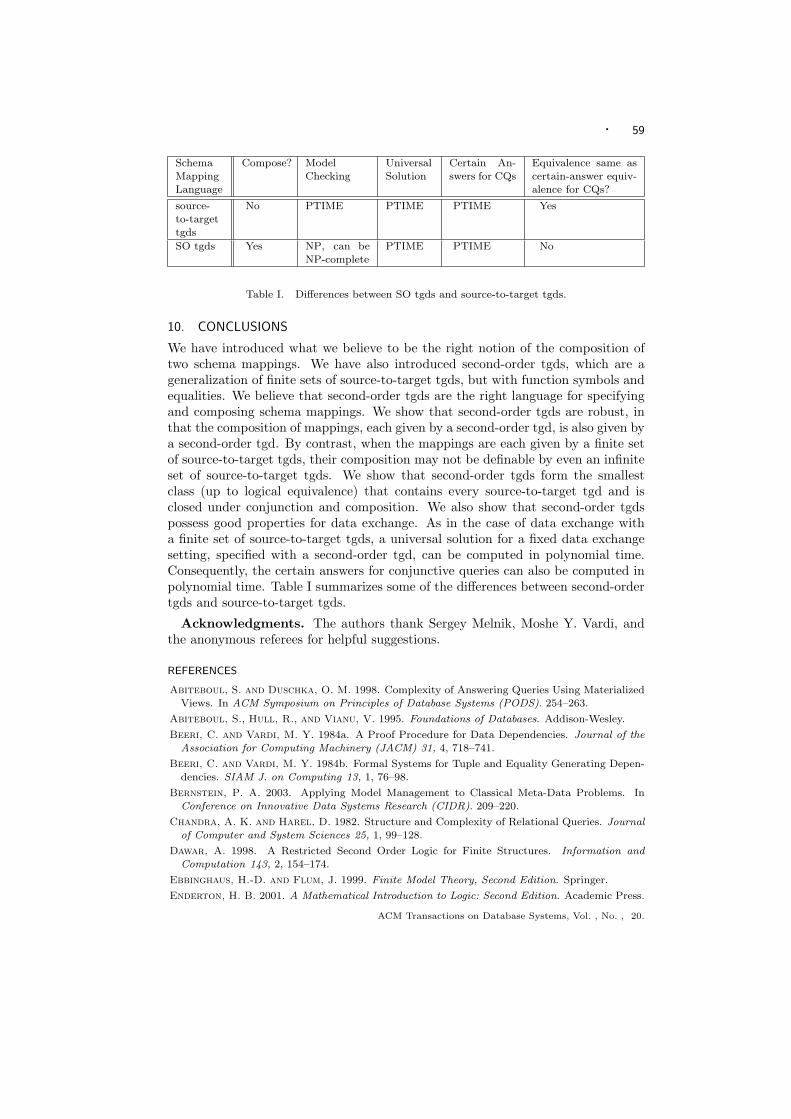
· 59

Schema

MappingLanguage

Compose? Model

Checking

Universal

Solution

Certain An-

swers for CQs

Equivalence same as

certain-answer equiv-alence for CQs?

source-

to-targettgds

No PTIME PTIME PTIME Yes

SO tgds Yes NP, can beNP-complete

PTIME PTIME No

Table I. Differences between SO tgds and source-to-target tgds.

10. CONCLUSIONS

We have introduced what we believe to be the right notion of the composition oftwo schema mappings. We have also introduced second-order tgds, which are ageneralization of finite sets of source-to-target tgds, but with function symbols andequalities. We believe that second-order tgds are the right language for specifyingand composing schema mappings. We show that second-order tgds are robust, inthat the composition of mappings, each given by a second-order tgd, is also given bya second-order tgd. By contrast, when the mappings are each given by a finite setof source-to-target tgds, their composition may not be definable by even an infiniteset of source-to-target tgds. We show that second-order tgds form the smallestclass (up to logical equivalence) that contains every source-to-target tgd and isclosed under conjunction and composition. We also show that second-order tgdspossess good properties for data exchange. As in the case of data exchange witha finite set of source-to-target tgds, a universal solution for a fixed data exchangesetting, specified with a second-order tgd, can be computed in polynomial time.Consequently, the certain answers for conjunctive queries can also be computed inpolynomial time. Table I summarizes some of the differences between second-ordertgds and source-to-target tgds.

Acknowledgments. The authors thank Sergey Melnik, Moshe Y. Vardi, andthe anonymous referees for helpful suggestions.

REFERENCES

Abiteboul, S. and Duschka, O. M. 1998. Complexity of Answering Queries Using Materialized

Views. In ACM Symposium on Principles of Database Systems (PODS). 254–263.

Abiteboul, S., Hull, R., and Vianu, V. 1995. Foundations of Databases. Addison-Wesley.

Beeri, C. and Vardi, M. Y. 1984a. A Proof Procedure for Data Dependencies. Journal of theAssociation for Computing Machinery (JACM) 31, 4, 718–741.

Beeri, C. and Vardi, M. Y. 1984b. Formal Systems for Tuple and Equality Generating Depen-

dencies. SIAM J. on Computing 13, 1, 76–98.

Bernstein, P. A. 2003. Applying Model Management to Classical Meta-Data Problems. InConference on Innovative Data Systems Research (CIDR). 209–220.

Chandra, A. K. and Harel, D. 1982. Structure and Complexity of Relational Queries. Journal

of Computer and System Sciences 25, 1, 99–128.

Dawar, A. 1998. A Restricted Second Order Logic for Finite Structures. Information and

Computation 143, 2, 154–174.

Ebbinghaus, H.-D. and Flum, J. 1999. Finite Model Theory, Second Edition. Springer.

Enderton, H. B. 2001. A Mathematical Introduction to Logic: Second Edition. Academic Press.


60 ·

Fagin, R. 1974. Generalized First-Order Spectra and Polynomial-Time Recognizable Sets. In

Complexity of Computation, SIAM-AMS Proceedings, Vol. 7, R. M. Karp, Ed. 43–73.

Fagin, R. 1982. Horn Clauses and Database Dependencies. Journal of the Association forComputing Machinery (JACM) 29, 4 (Oct.), 952–985.

Fagin, R., Kolaitis, P. G., Miller, R. J., and Popa, L. 2005. Data Exchange: Semantics and

Query Answering. Theoretical Computer Science 336, 89–124. Preliminary version in Proc.

2003 International Conference on Database Theory, pp. 207–224.

Fagin, R., Kolaitis, P. G., and Popa, L. 2003. Data Exchange: Getting to the Core. InACM Symposium on Principles of Database Systems (PODS). 90–101. To appear in ACM

Transactions on Database Systems.

Fagin, R., Kolaitis, P. G., Popa, L., and Tan, W.-C. 2004. Composing Schema Mappings:Second-Order Dependencies to the Rescue. In ACM Symposium on Principles of Database

Systems (PODS). 83–94.

Feder, T. and Vardi, M. 1998. The Computational Structure of Monotone Monadic SNP and

Constraint Satisfaction: A Study through Datalog and Group Theory. SIAM J. on Comput-ing 28, 57–104. Preliminary version in Proc. 25th ACM Symp. on Theory of Computing, May

1993, pp. 612–622.

Garey, M., Johnson, D. S., and Stockmeyer, L. J. 1976. Some simplified NP-complete graphproblems. Theoretical Computer Science 1, 237–267.

Halevy, A. Y., Ives, Z. G., Mork, P., and Tatarinov, I. 2003. Piazza: Data Management

Infrastructure for Semantic Web Applications. In International World Wide Web Conference.

556–567.

Immerman, N. 1999. Descriptive Complexity. Springer.

Lenzerini, M. 2002. Data Integration: A Theoretical Perspective. In ACM Symposium on

Principles of Database Systems (PODS). 233–246.

Madhavan, J. and Halevy, A. Y. 2003. Composing Mappings Among Data Sources. In Inter-

national Conference on Very Large Data Bases (VLDB). 572–583.

Miller, R. J., Haas, L. M., and Hernandez, M. 2000. Schema Mapping as Query Discovery.In International Conference on Very Large Data Bases (VLDB). 77–88.

Popa, L., Velegrakis, Y., Miller, R. J., Hernandez, M. A., and Fagin, R. 2002. Translating

Web Data. In International Conference on Very Large Data Bases (VLDB). 598–609.

Vassiliadis, P., Simitsis, A., and Skiadopoulos, S. 2002. On the Logical Modeling of ETL Pro-cesses. In International Conference on Advanced Information Systems Engineering (CAiSE).

782–786.


composing schema mappings: second-order dependencies to ... · composing schema mappings:...

Documents