class bfs 1209045147137930
TRANSCRIPT
[鍵入文字]
Classical Electrodynamics
Chapter 6
Maxwell Equations ,
Macroscopic Electromagnetism,
Conservation Law
2011 Classical Electrodynamics Prof. Y. F. Chen
[鍵入文字]
Contents
§6.1Maxwell Equations
§6.2Conservation law
2011 Classical Electrodynamics Prof. Y. F. Chen
[鍵入文字]
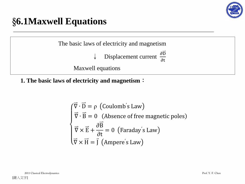
§6.1Maxwell Equations
The basic laws of electricity and magnetism
↓ Displacement current
Maxwell equations
1. The basic laws of electricity and magnetism:
2011 Classical Electrodynamics Prof. Y. F. Chen
[鍵入文字]
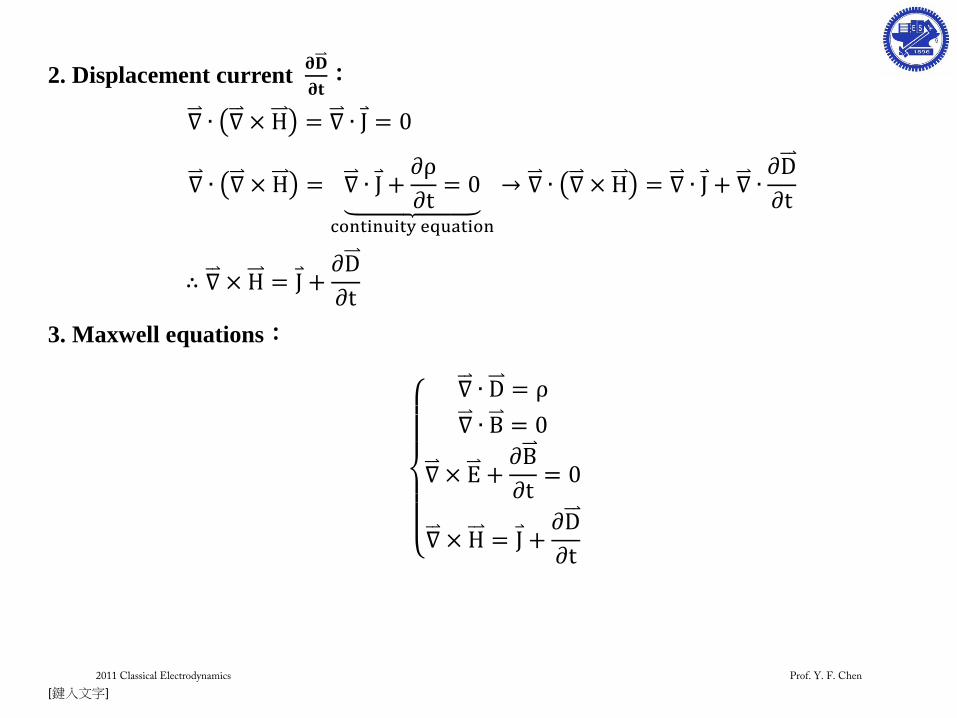
2. Displacement current
:
3. Maxwell equations:
2011 Classical Electrodynamics Prof. Y. F. Chen
[鍵入文字]
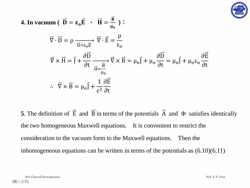
4. In vacuum ( 、
):
5. The definition of and in terms of the potentials and satisfies identically
the two homogeneous Maxwell equations. It is convenient to restrict the
consideration to the vacuum form to the Maxwell equations. Then the
inhomogeneous equations can be written in terms of the potentials as (6.10)(6.11)
2011 Classical Electrodynamics Prof. Y. F. Chen
[鍵入文字]
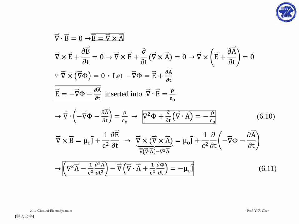
,Let
inserted into
(6.10)
(6.11)
2011 Classical Electrodynamics Prof. Y. F. Chen
[鍵入文字]
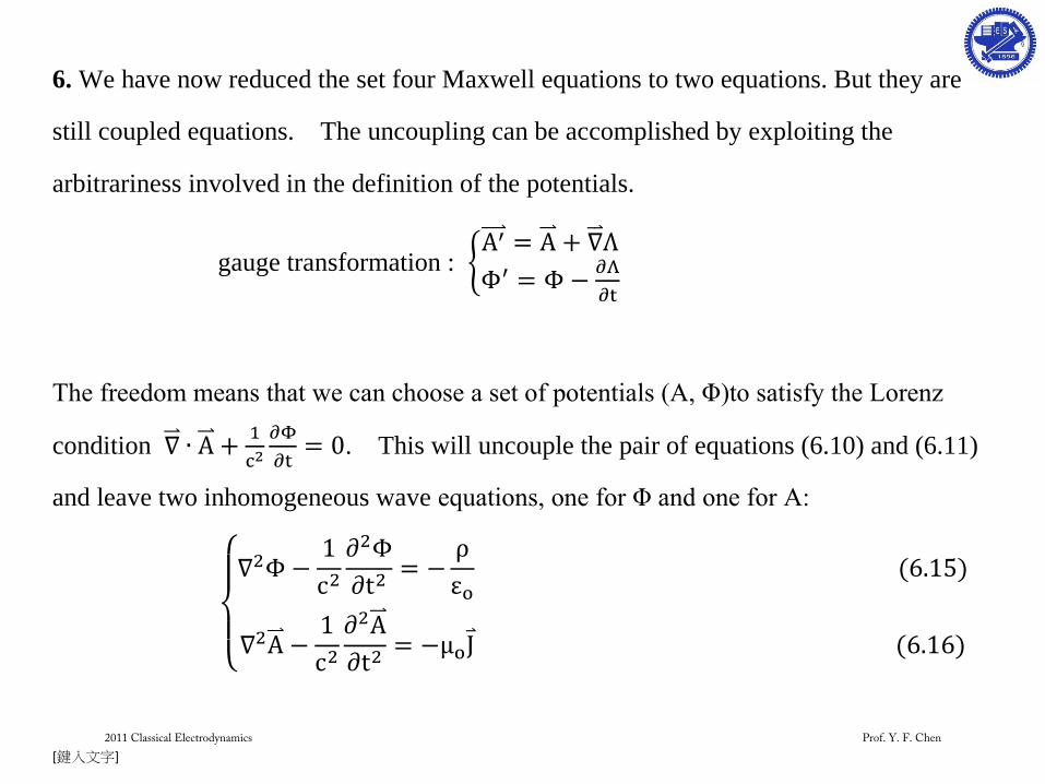
6. We have now reduced the set four Maxwell equations to two equations. But they are
still coupled equations. The uncoupling can be accomplished by exploiting the
arbitrariness involved in the definition of the potentials.
gauge transformation :
The freedom means that we can choose a set of potentials (A, Φ)to satisfy the Lorenz
condition
. This will uncouple the pair of equations (6.10) and (6.11)
and leave two inhomogeneous wave equations, one for Φ and one for A:
2011 Classical Electrodynamics Prof. Y. F. Chen
[鍵入文字]
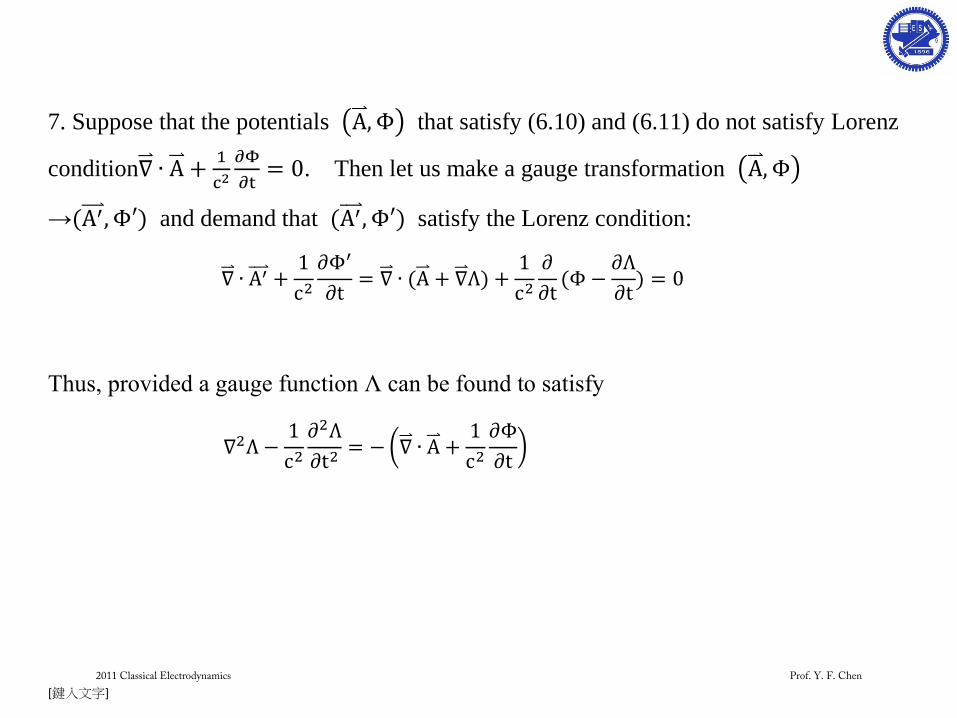
7. Suppose that the potentials that satisfy (6.10) and (6.11) do not satisfy Lorenz
condition
. Then let us make a gauge transformation
→ and demand that satisfy the Lorenz condition:
Thus, provided a gauge function Λ can be found to satisfy
2011 Classical Electrodynamics Prof. Y. F. Chen
[鍵入文字]
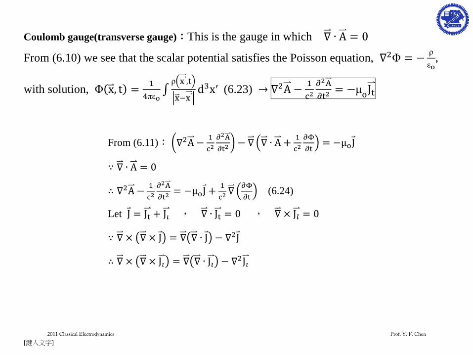
Coulomb gauge(transverse gauge):This is the gauge in which
From (6.10) we see that the scalar potential satisfies the Poisson equation, Φ
,
with solution, Φ
(6.23)
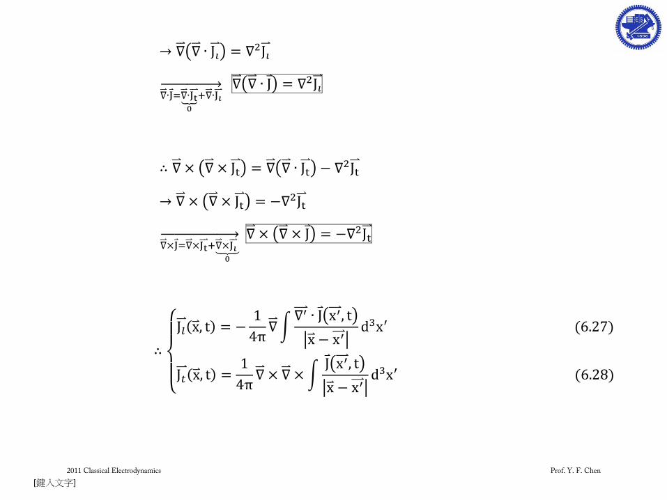
From (6.11):
(6.24)
Let , ,
2011 Classical Electrodynamics Prof. Y. F. Chen
[鍵入文字]
2011 Classical Electrodynamics Prof. Y. F. Chen
[鍵入文字]
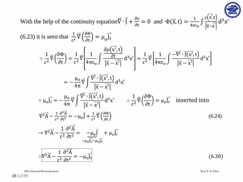
With the help of the continuity equation
and Φ
(6.23) it is seen that
Φ
(6.24)
2011 Classical Electrodynamics Prof. Y. F. Chen

[鍵入文字]
※In passing we note a peculiarity of the Coulomb gauge. It is well known that
electromagnetic disturbances propagate with finite speed. Yet (6.23) indicates that the
scalar potential “propagates” instantaneously everywhere in space. The vector potential,
on the other hand, satisfies the wave equation (6.30), with its implied finite speed of
propagation c. At first glance it is puzzling to see how obviously unphysical behavior is
avoided. A preliminary remark is that it is the fields, not the potentials, that concern us.
A further observation is that the transverse current (6.28) extends over all space, even
if J is localized.
2011 Classical Electrodynamics Prof. Y. F. Chen
[鍵入文字]
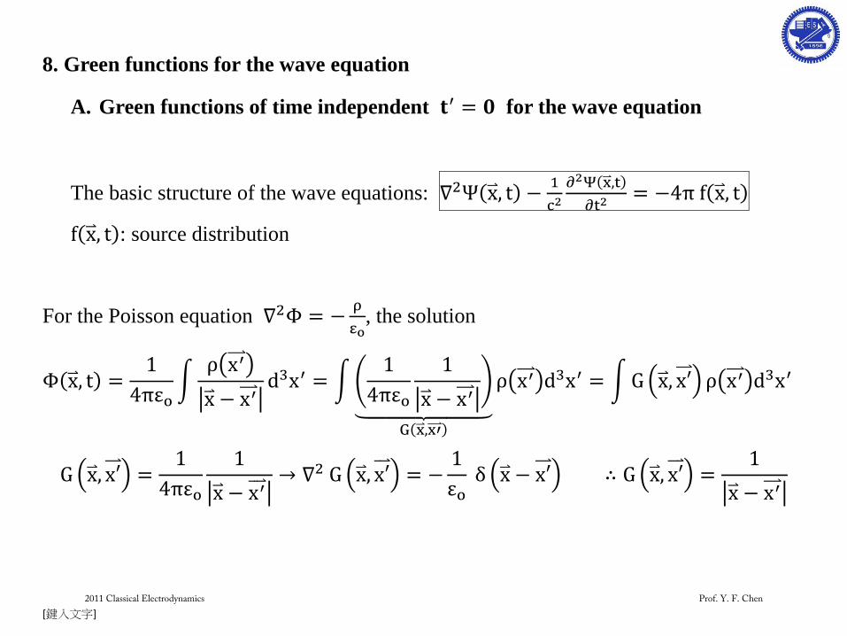
8. Green functions for the wave equation
A. Green functions of time independent for the wave equation
The basic structure of the wave equations:
: source distribution
For the Poisson equation
, the solution
2011 Classical Electrodynamics Prof. Y. F. Chen
[鍵入文字]
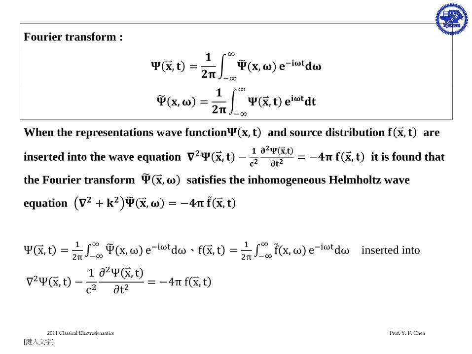
Fourier transform :
When the representations wave function and source distribution are
inserted into the wave equation
it is found that
the Fourier transform satisfies the inhomogeneous Helmholtz wave
equation
、
inserted into
2011 Classical Electrodynamics Prof. Y. F. Chen
[鍵入文字]
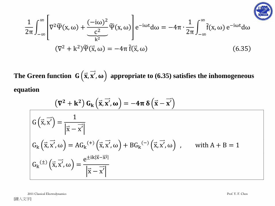
The Green function appropriate to (6.35) satisfies the inhomogeneous
equation
2011 Classical Electrodynamics Prof. Y. F. Chen
[鍵入文字]
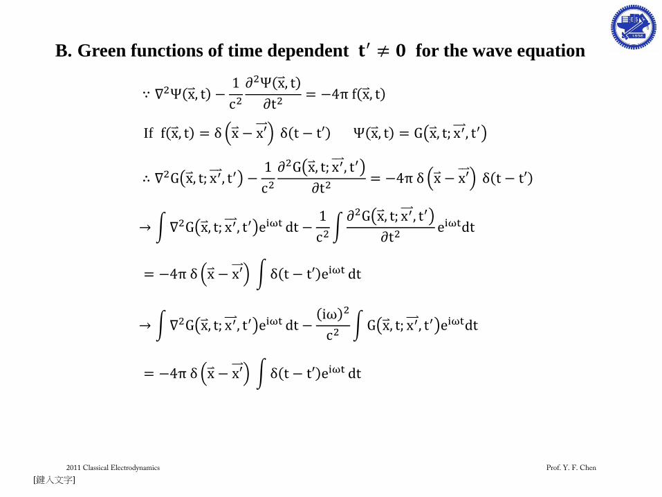
B. Green functions of time dependent for the wave equation
If
2011 Classical Electrodynamics Prof. Y. F. Chen
[鍵入文字]
2011 Classical Electrodynamics Prof. Y. F. Chen
[鍵入文字]
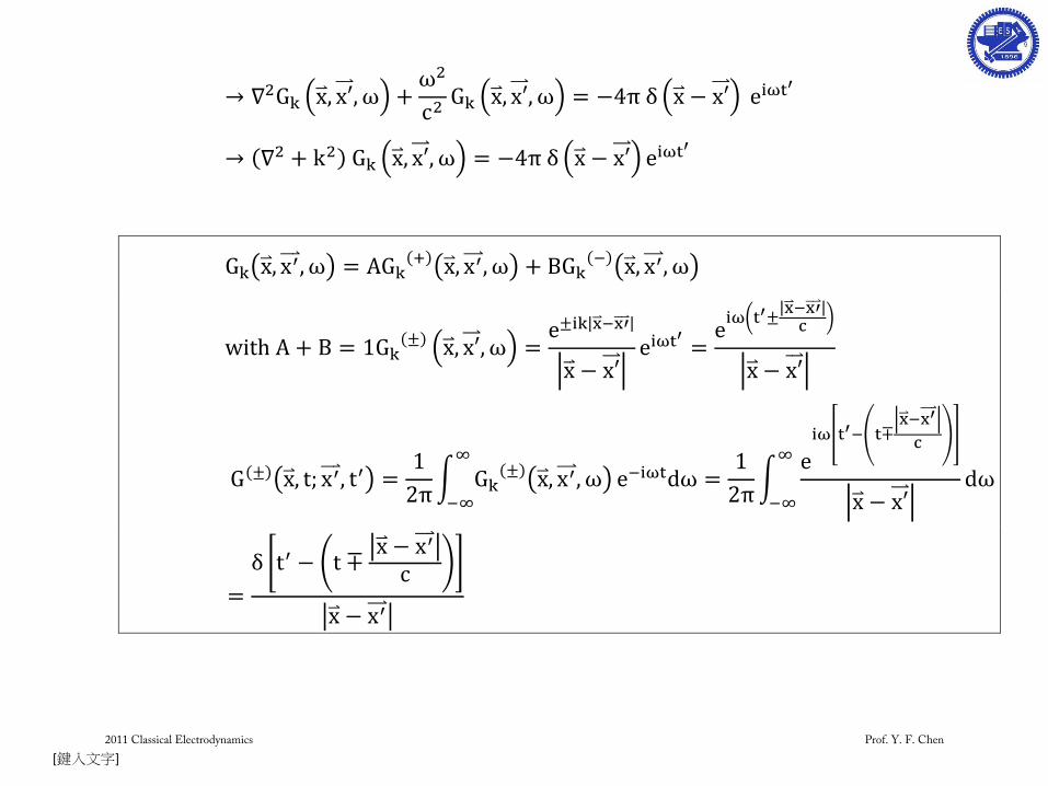
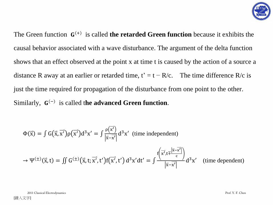
The Green function is called the retarded Green function because it exhibits the
causal behavior associated with a wave disturbance. The argument of the delta function
shows that an effect observed at the point x at time t is caused by the action of a source a
distance R away at an earlier or retarded time, t’ = t − R/c. The time difference R/c is
just the time required for propagation of the disturbance from one point to the other.
Similarly, is called the advanced Green function.
(time independent)
(time dependent)
2011 Classical Electrodynamics Prof. Y. F. Chen
[鍵入文字]
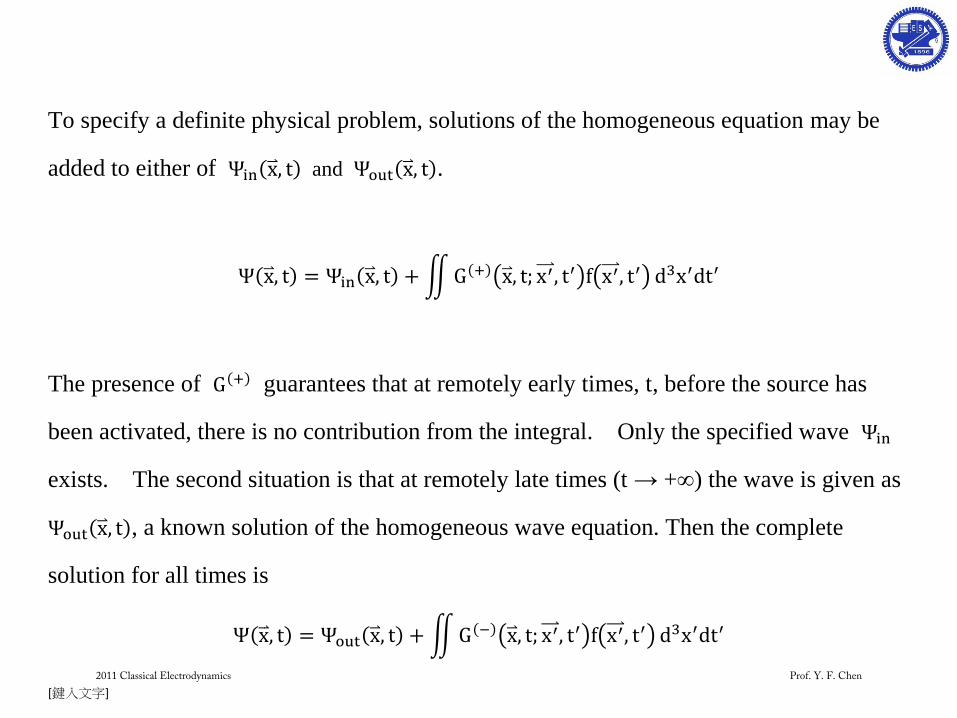
To specify a definite physical problem, solutions of the homogeneous equation may be
added to either of and .
The presence of guarantees that at remotely early times, t, before the source has
been activated, there is no contribution from the integral. Only the specified wave
exists. The second situation is that at remotely late times (t → +∞) the wave is given as
, a known solution of the homogeneous wave equation. Then the complete
solution for all times is
2011 Classical Electrodynamics Prof. Y. F. Chen
[鍵入文字]
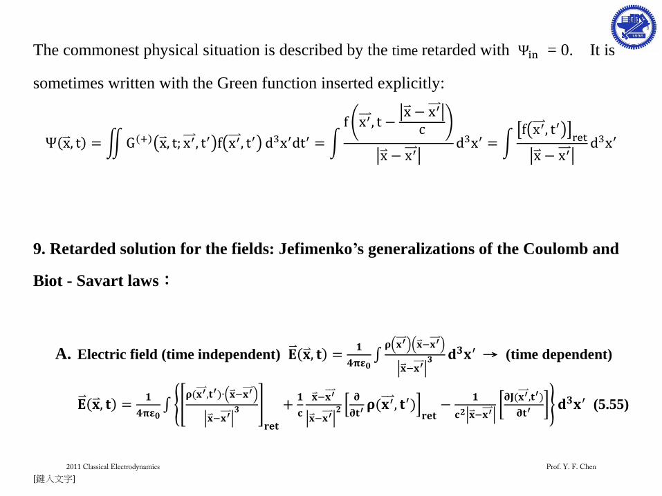
The commonest physical situation is described by the time retarded with = 0. It is
sometimes written with the Green function inserted explicitly:
9. Retarded solution for the fields: Jefimenko’s generalizations of the Coulomb and
Biot - Savart laws:
A. Electric field (time independent)
→ (time dependent)
(5.55)
2011 Classical Electrodynamics Prof. Y. F. Chen
[鍵入文字]
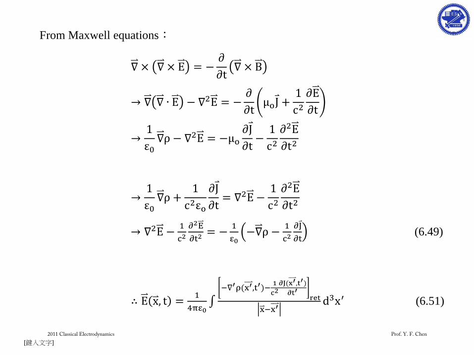
From Maxwell equations:
(6.49)
(6.51)
2011 Classical Electrodynamics Prof. Y. F. Chen
[鍵入文字]
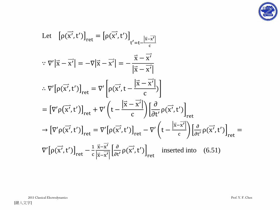
Let
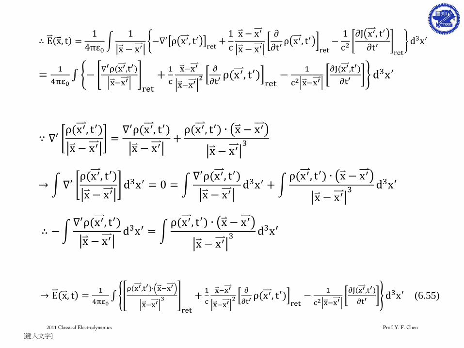
inserted into (6.51)
2011 Classical Electrodynamics Prof. Y. F. Chen
[鍵入文字]
(6.55)
2011 Classical Electrodynamics Prof. Y. F. Chen
[鍵入文字]
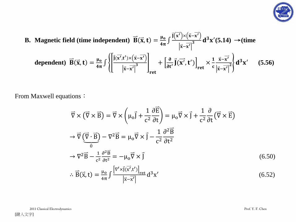
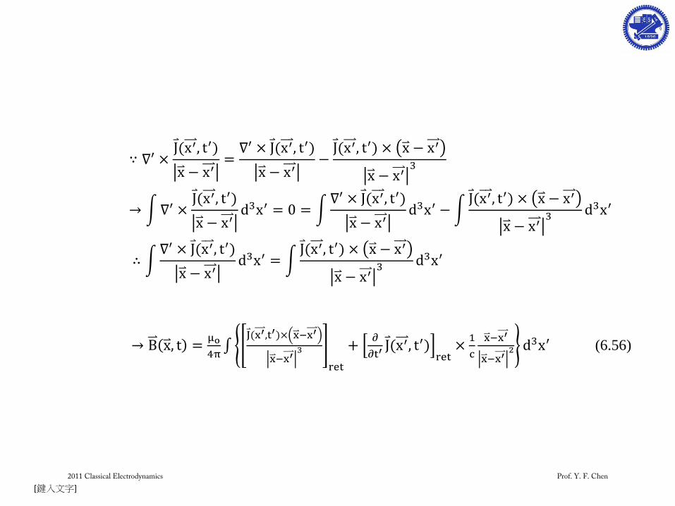
B. Magnetic field (time independent)
(5.14) →(time
dependent)
(5.56)
From Maxwell equations:
(6.50)
(6.52)
2011 Classical Electrodynamics Prof. Y. F. Chen
[鍵入文字]
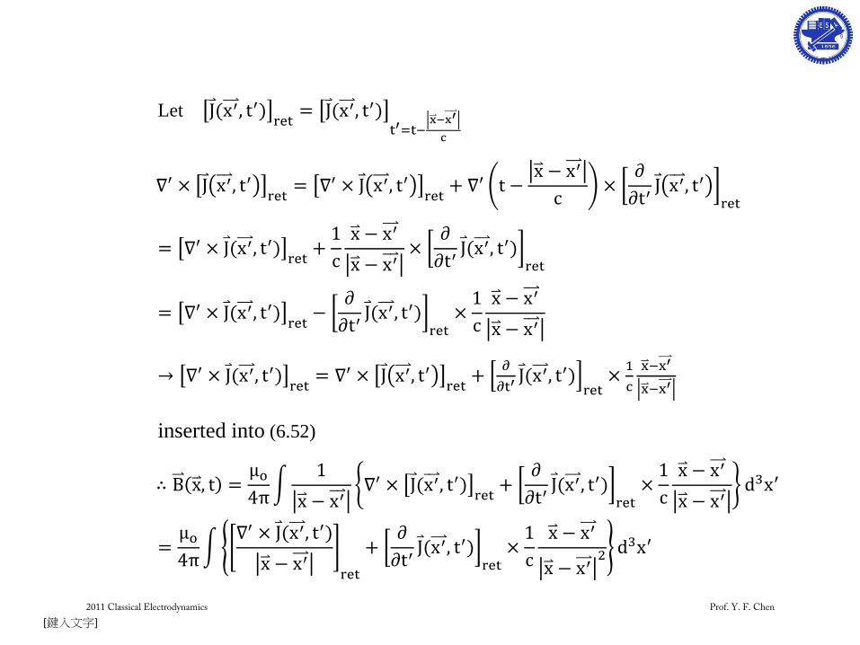
Let
inserted into (6.52)
2011 Classical Electrodynamics Prof. Y. F. Chen
[鍵入文字]
(6.56)
2011 Classical Electrodynamics Prof. Y. F. Chen
[鍵入文字]
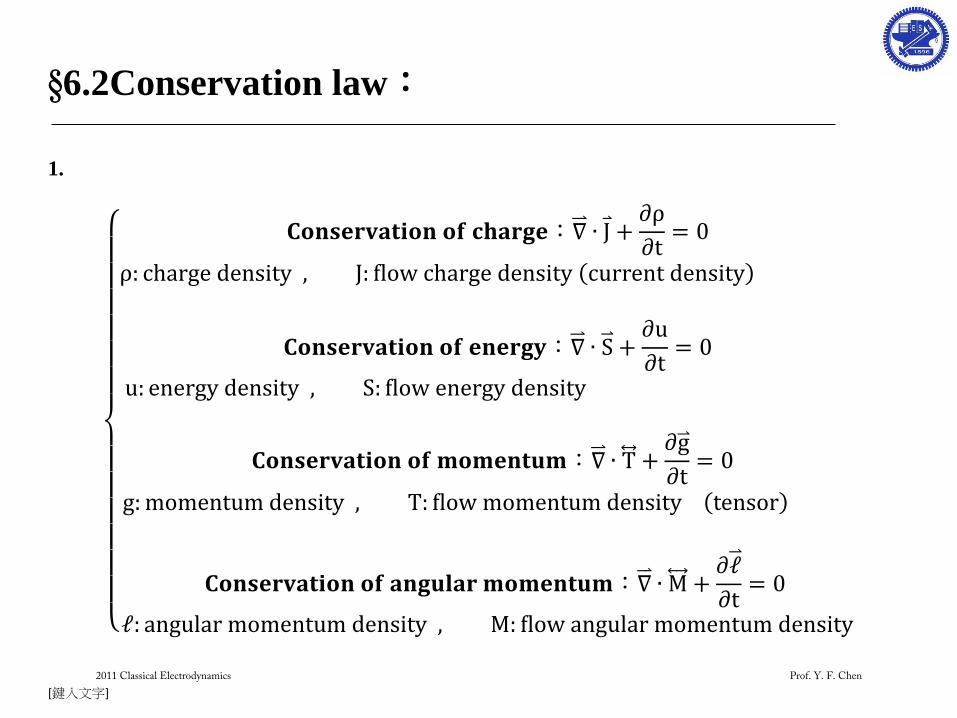
§6.2Conservation law:
1.
:
:
:
:
2011 Classical Electrodynamics Prof. Y. F. Chen
[鍵入文字]
2011 Classical Electrodynamics Prof. Y. F. Chen
[鍵入文字]
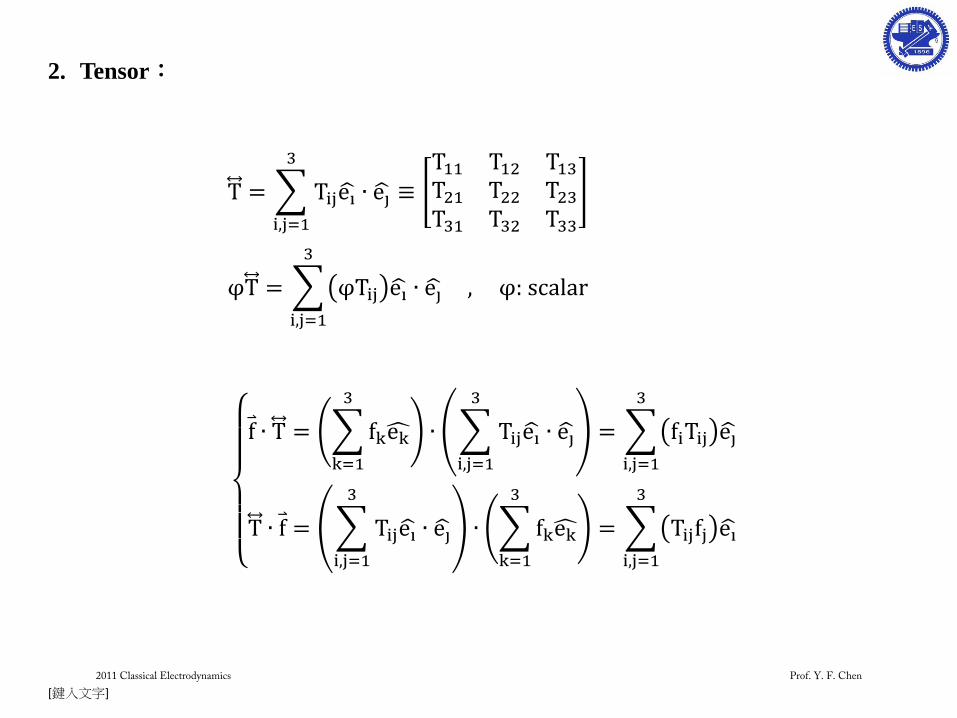
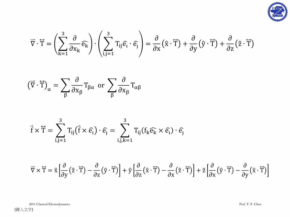
2. Tensor:
2011 Classical Electrodynamics Prof. Y. F. Chen
[鍵入文字]
2011 Classical Electrodynamics Prof. Y. F. Chen
[鍵入文字]
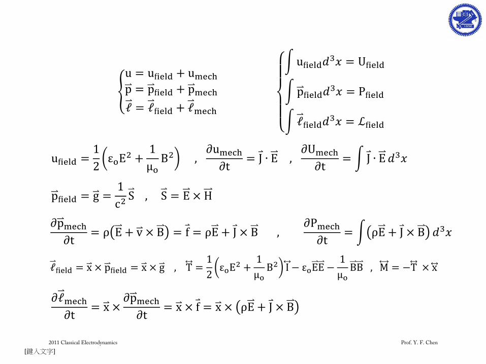
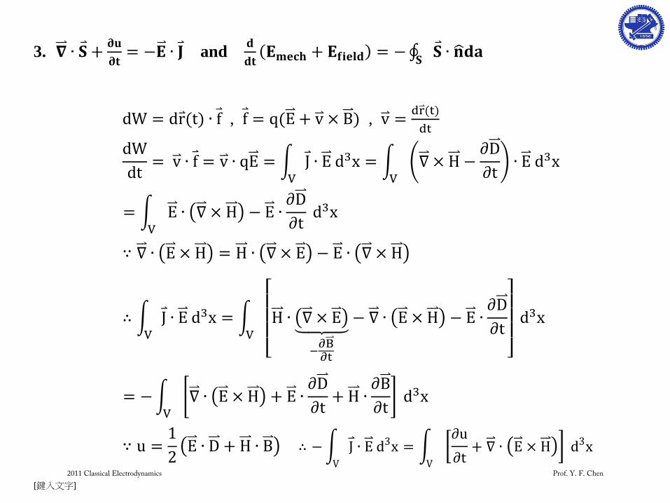
3.
and
, ,
2011 Classical Electrodynamics Prof. Y. F. Chen
[鍵入文字]
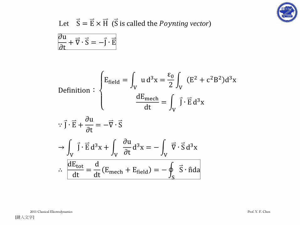
Let ( ting vector)
:
2011 Classical Electrodynamics Prof. Y. F. Chen
[鍵入文字]
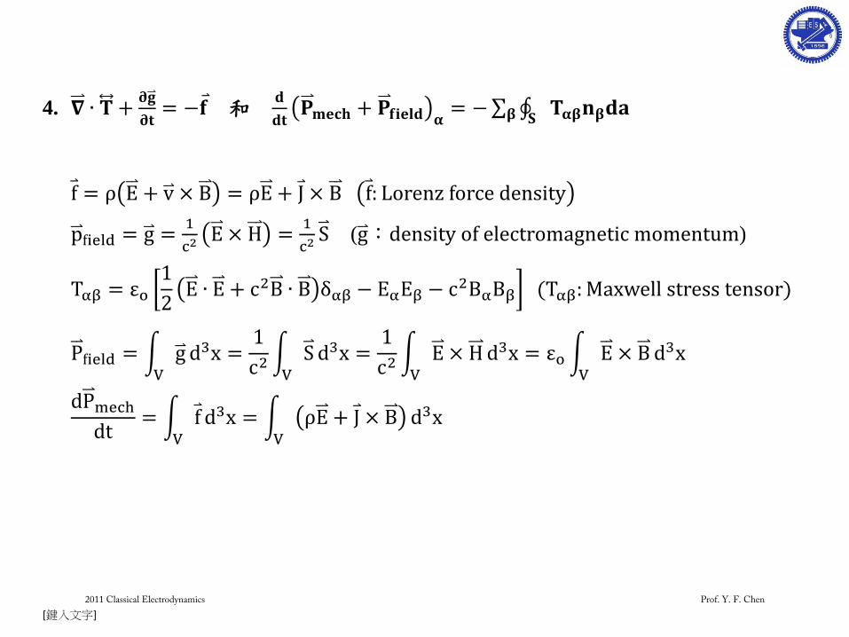
4.
和
( : )
2011 Classical Electrodynamics Prof. Y. F. Chen
[鍵入文字]
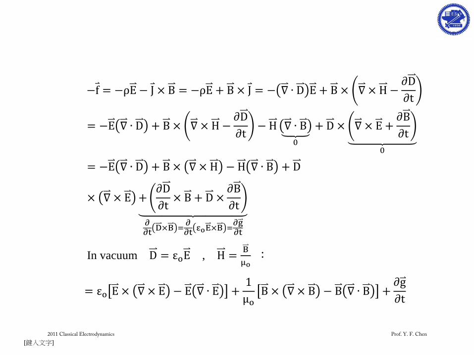
In vacuum ,
:
2011 Classical Electrodynamics Prof. Y. F. Chen
[鍵入文字]
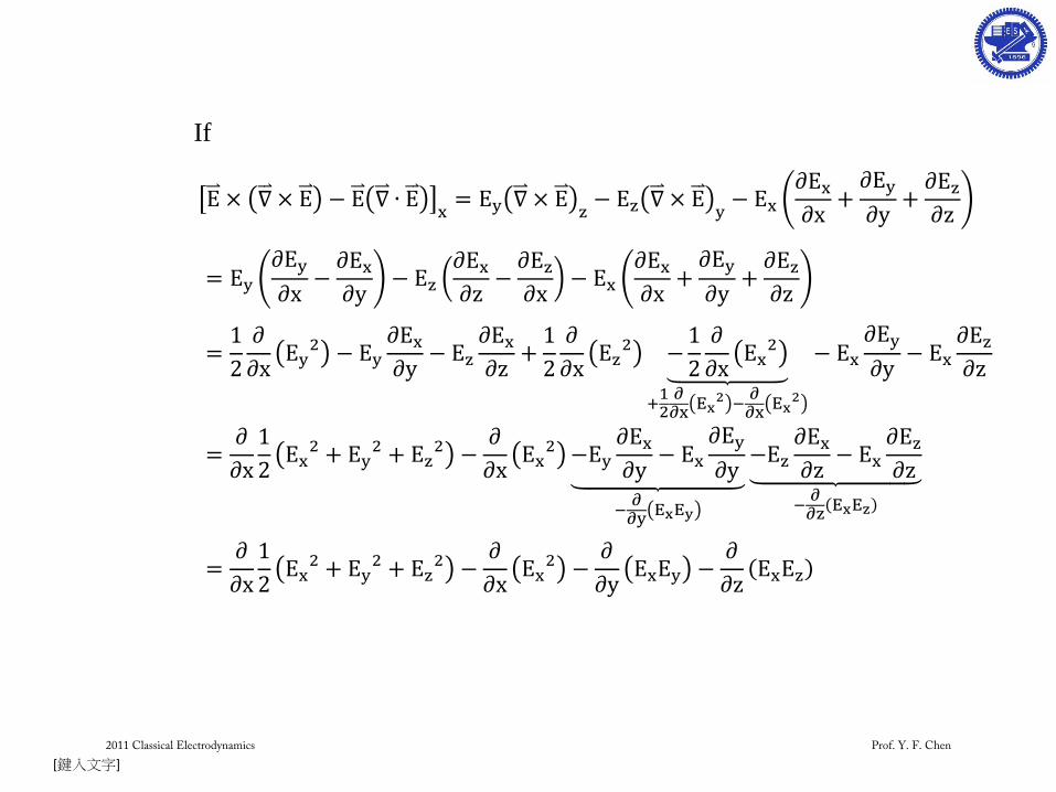
If
2011 Classical Electrodynamics Prof. Y. F. Chen
[鍵入文字]
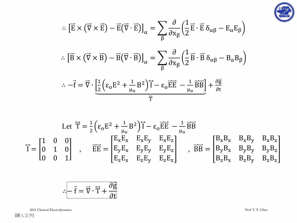
Let
,
,
2011 Classical Electrodynamics Prof. Y. F. Chen
[鍵入文字]
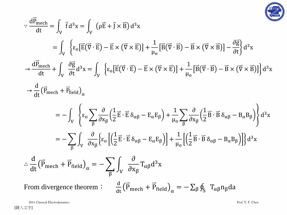
From divergence theorem:
2011 Classical Electrodynamics Prof. Y. F. Chen
[鍵入文字]
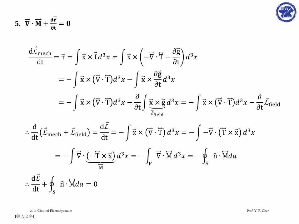
5.
2011 Classical Electrodynamics Prof. Y. F. Chen