bidding for incomplete contracts: an empirical analysis...
TRANSCRIPT
Bidding for Incomplete Contracts: An Empirical Analysis of
Adaptation Costs∗
Patrick Bajari
University of Minnesota and NBER
Stephanie Houghton
Texas A&M University
Steven Tadelis
UC Berkeley
March 19, 2012
Abstract
Procurement contracts are often renegotiated because of changes that are required after their
execution. Using highway paving contracts we show that renegotiation imposes significant
adaptation costs. Reduced form regressions suggest that bidders respond strategically to con-
tractual incompleteness and that adaptation costs are an important determinant of their bids.
A structural empirical model compares adaptation costs to bidder markups and shows that
adaptation costs account for 8-14 percent of the winning bid. Markups from private infor-
mation and market power, the focus of much of the auctions literature, are much smaller by
comparison. Implications for government procurement are discussed. JEL classifications: D23,
D82, H57, L14, L22, L74.
∗We thank Liran Einav, Phil Haile, Igal Hendel, Ali Hortacsu, Tom Hubbard, Jon Levin and especially
Ken Hendricks, Han Hong and Harry Paarsch for helpful discussions. We are grateful for financial support
from the National Science Foundation.
Page 1 of 48
1 Introduction
The benefits of using auctions to procure goods and services are well known and vigorously
advocated. Competitive bidding results in low prices and limits favoritism. Employing
auctions to procure standard goods such as pencils, printers and book-keeping software is
straightforward, yet procuring custom made goods and services to fit a buyer’s unique needs
poses challenges. First, the buyer must spend resources to translate operational needs into
well defined and communicable specifications. Second, needs for adaptations and changes
often result from inadequate designs and specifications, changes in the external environment,
or more generally, the extent to which the initial contract is incomplete.
Incomplete contracts force the buyer and supplier to negotiate adaptations both to the
scope of work and to compensation, which may result in considerable discrepancies between
the winning bid and the final payment. A well known example is the “Big Dig” highway
artery in Boston, for which 12,000 changes to more than 150 contracts led to $1.6 billion in
cost overruns, most of which can be traced back to unsatisfactory design.1 One source of
cost overruns is the additional work that was not anticipated. In addition, adaptation costs
are incurred by disruptions to the normal flow of work that could have been avoided with
adequate planning in advance. Renegotiating the contract also generates adaptation costs
in the form of haggling, dispute resolution and opportunistic behavior.
Despite the prevalence of incomplete contracts, their effect on procurement in general,
and on adaptation costs in particular are ignored almost without exception in both the
theoretical and empirical auction literatures. This paper contributes by offering a first
attempt to measure the economic costs of ex post adaptations that result from incomplete
contracts. We develop a simple framework of bidding for incomplete contracts and apply it
to highway procurement in the state of California. Our analysis suggests that adaptation
costs are large, imposing significant extra costs on public procurement.
Our approach is guided by three important features of highway procurement. First, given
the competitive nature of the highway construction industry (publicly traded firms in our
sample report profit margins of less than 3 percent), bidders must anticipate ex post changes
and try to include any adaptation costs in their bids. Second, highway procurement uses
“unit-price auctions” where contracts are summarized by a list of estimated input quantities
1According to the Boston Globe, “About $1.1 billion of that can be traced back to deficiencies in
the designs, records show: $357 million because contractors found different conditions than appeared
on the designs, and $737 million for labor and materials costs associated with incomplete designs.” See
http://www.boston.com/news/specials/bechtel/part_1/.
2
Page 2 of 48
required to do the job. A bidder submits a list of itemized (unit) prices, which multiplied
by estimated quantities result in the bidder’s total bid. The contractor with the lowest total
bid wins the auction. Third, the winning total bid is seldom equal to the final compensation
because ex ante estimated quantities and ex post actual quantities never perfectly agree.
Furthermore, changes in scope may be necessary when some specifications of the project
need to be altered.
We develop a stylized model where contractors form rational expectations about the
ways in which actual quantities will differ from estimated ones, as well as whether changes
in scope will be required. Hence, expected changes in payments and adaptation costs will be
incorporated into the bids ex ante.2 We then apply the empirical framework of our model to
a panel data set of highway contract bids that we have collected from Caltrans (California’s
Department of Transportation). The data includes bidder identities, bids, detailed cost
estimates, and measures of cost advantages. Unlike most studies of procurement, our data
also contains detailed information on how the initial designs were altered, including both
estimated and actual quantities for all work items in the contract, as well as payments to
the contractor from changes in scope.
Our empirical analysis first presents reduced form estimations where the strategy for
identifying adaptation costs is based on our theoretical model. Suppose that the contractors
all expect additional payments due to ex post changes. Controlling for production costs,
if there were no adaptation costs then competition implies that for every extra dollar of
profits, each contractor should lower its bid by exactly one dollar. If the regression is
correctly specified, the coefficient on ex post additional payments should therefore be −1.We find that some coefficients are closer to +1, implying that ex post changes on net
generate more costs than revenue. Our estimates suggest that adaptation costs, which have
until now been largely ignored, are substantial–on average they are between eight and
fourteen percent of the winning bid.
A concern with our identification strategy is that complex projects, for which ex post
changes are likely, also have higher production costs. This would confound adaptation costs
with production costs and curtail our results. We address this concern using an instrumental
variables strategy and identify an exogenous shifter of ex post payments that is uncorrelated
with project characteristics. As we explain in section 4.3, we use the identity of the Caltrans
2This is in line with Haile (1991) who explores timber auctions where forward looking rational bidders
take into account the future possibility of resale to calculate their optimal bid.
3
Page 3 of 48
engineer assigned to the project as an instrument for changes to compensation. Individual
engineers have discretion over ex post adjustments, making some engineers easier to work
with while others are known to cause problems. Engineers are randomly assigned to manage
several projects and their identities are known to contractors at the time of bidding, allowing
us to identify adaptation costs using engineer assignments.
In order to quantify the magnitude of adaptation costs as a markup over production
costs, we estimate a structural model that builds on our theoretical analysis and decomposes
markups into three components. First, as in any auction model, markups are a function of
private information and local market power. Second, as in Athey and Levin (2001), who
investigate behavior in unit-price timber auctions, we estimate the impact of “unbalanced”
bids. Namely, contractors can increase expected profits by increasing (decreasing) unit
prices on items that are expected to overrun (under-run). Third, we estimate the adaptation
costs from changes to the initial specifications (estimated quantities) to uncover the ex post
costs of misspecified ex ante designs. The structural model estimates are consistent with
the reduced form findings and show that adaptation costs are larger than the other two
mark-up drivers. We conclude our empirical analysis with a conservative bounding strategy
to find upper and lower bounds on the adaptation costs. We continue to find large and
significant estimates of adaptation costs under these two specifications, and conclude that
our estimates suggest that adaptation and changes are a major determinant of bids in this
industry and an important potential source of inefficiency.
While largely ignored in the empirical procurement literature, concerns over the impact
of adaptation costs are prevalent in the construction management literature (See Hinze
(1993), Clough and Sears (1994), and Sweet (1994)). The earliest foundations of transac-
tion costs economics (Williamson (1971)) argue that incomplete contracts imply both needs
for adaptation and potential frictions. This idea has been explored in the procurement liter-
ature, and several studies emphasize the importance of adaptation costs including Crocker
and Reynolds (1993), Bajari and Tadelis (2001) and Chakravarty and MacLeod (2009).
Our paper contributes to this literature because, to the best of our knowledge, there are
no empirical estimates of the dollar value of these costs. We demonstrate that standard
methods for estimating auctions can be modified to yield an estimate of adaptation costs
in procurement auctions.
This paper also contributes to the literature on structural estimation of auctions (See,
e.g., Paarsch (1992), Guerre, Perrigne and Vuong (2000) and Krasnokutskaya (2011).) First,
4
Page 4 of 48

our estimates imply that adaptation costs, which have until now been largely ignored, seem
to impose more distortions and frictions as compared with market power and unbalanced
bidding. Second, our results suggest that profit markups in standard bidding models are
often misspecified because they do not account for the discrepancies between initial bids
and final payments, omitting important parts of a contractor’s revenues and costs. This in
turn implies that policies geared towards reducing the amount of contractual incompleteness
may have large benefits by reducing the costs of public procurement.
2 Competitive Bidding for Highway Contracts
Highway construction, as well as other public sector procurement, is often done using unit-
price contracts. (See, e.g., Hinze (1993).) Government engineers first prepare a list of items
that describe the tasks and materials required for the job. In the contracts we study,
items include laying asphalt, installing new sidewalks and striping the highway. For each
work item, engineers provide an estimate of the quantity needed to complete the job. For
example, they might estimate 25,000 tons of asphalt, 10,000 square yards of sidewalk and
50 rumble strips. The itemized list is publicly advertised along with a detailed set of plans
and specifications that describe how the project is to be completed.
An interested contractor will bid per unit prices for each work item on the engineer’s
list. Figure 1 shows an example of the structure of a completed bid, which must be sealed
and submitted prior to a set date. When the bids are opened, the contract is awarded
to the contractor with the lowest estimated total bid, defined as the sum of the estimated
individual line item bids.3
Item Description Estimated Quantity Per Unit Bid Estimated Item Bid
1. asphalt (tons) 25,000 $25.00 $625,000.00
2. sidewalk (square feet) 10,000 $9.00 $90,000.00
3. rumble strips 50 $5.00 $250.00
Total Bid: $715,250.00
Figure 1: Unit Price Contract—An Example.
Actual quantities will almost always be different from estimated quantities. The dif-
ference may be substantial if there are unexpected conditions or work has to be redone or
3The lowest bid can be rejected if the bidder is not appropriately bonded or does not have a sufficient
amount of work awarded to disadvantaged business enterprises as subcontractors. Also, bids judged to be
highly unbalanced can be rejected, as discussed further below.
5
Page 5 of 48
eliminated. As a result, final payments made to the contractor are almost never equal to
the original bid, and their determination can be complicated. Caltrans’ Standard Specifica-
tions and its Construction Manual discuss the determination of the final payment. To a
first approximation, there are three primary reasons for modifying the payments away from
the simple sum of actual unit costs.
First, if the difference between estimated and actual quantities is large, or if it is thought
to be due to negligence by one party, both sides will renegotiate an adjustment of compen-
sation.4 Using our example, if the asphalt ran over by 10,000 tons, Caltrans would hesitate
to pay an extra $250,000, and the parties may negotiate an adjustment to lower the total
bill. In our data, adjustments are recorded as a lump sum change, but this may also be a
way for parties to adjust the implied unit price on a particular item.
Second, there may be a change in scope. For instance, the original scope might be to
resurface 2 miles of highway. However, the engineers and contractor might discover that
the subsurface is not stable and that certain sections need to be excavated and have gravel
added, an activity that was not originally described. In most cases, the contractor and
Caltrans will negotiate a change order that amends the scope of the contract as well as
the final payment. If negotiations break down, this may lead to arbitration or a lawsuit.
Payments from changes will appear in two ways. One is that changes in the actual ex post
quantities of pre-specified items will be compensated for through the unit prices. Another
is by extra payments may to reflect the use of unanticipated materials or other adjustment
costs, and they are recorded as extra work in our data.
Finally, the payment may be altered because of deductions. If work is not completed on
time or if it fails to meet specifications, Caltrans may deduct liquidated damages. Such de-
ductions are often a source of disputes between Caltrans and the contractor. The contractor
may argue that the source of the delay is poor planning or inadequate specifications pro-
vided by Caltrans, while Caltrans might argue that the contractor’s negligence is the source
of the problem. The final deductions imposed may be the outcome of heated negotiations
or even lawsuits and arbitrations between contractors and Caltrans.
It is widely believed in the industry that some contractors attempt to strategically
manipulate their bids in anticipation of changes to the payment. Contractors read the
plans and specifications to forecast the likelihood and magnitude of changes to the contract.
4 In the particular case of highway construstion procured by Caltrans, this type of adjustment is called
for if the actual quantity of an item varies from the engineer’s estimate by 25 percent or more.
6
Page 6 of 48

For instance, consider the example of Figure 1, in which the total bid is $715,250. Suppose
that after reading the plans and specifications, the contractor expects asphalt to overrun by
5,000 tons and sidewalk to under-run by 3,000 square feet. If he changes his bid on sidewalk
to $5.00 and his bid on asphalt to $26.60 then his total bid will be unchanged. However,
this will increase the contractors’ expected total payment to $833,750.00 (266× 30 000 +5 × 7000 + 5 × 50) compared to $813,750.00 when bids of $25.00 and $9.00 are entered.This increases his total payment without increasing his total bid, fixing his probability of
winning. A bid is referred to as unbalanced if it has unusually high unit prices on some items
(expected to overrun) and unusually low unit prices on others (expected to under-run).
Athey and Levin (2001) note that the optimal strategy for a risk neutral contractor is
to submit a bid that has zero unit prices for some items that are overestimated, and put all
the actual costs on items that are underestimated. In the data, however, while zero unit
price bids have been observed, they are very uncommon. Athey and Levin suggest that
one reason for this is risk aversion. After speaking with industry participants and reading
industry sources we believe that for construction contracts other considerations are more
important. In particular, Caltrans is not required to accept the low bid if it is deemed
to be irregular (see Sweet (1994) for an in depth discussion of irregular bids). A highly
unbalanced bid is a sufficient condition for a bid to be deemed irregular. As a result, a bid
with a zero unit price is very likely, if not certain, to be rejected.5
Also, the Standard Specifications and the Construction Manual indicate that unit prices
on items that overrun by more than 25 percent are open to renegotiation. In these ne-
gotiations, Caltrans engineers will attempt to estimate a fair market value for a particular
unit price based on bids submitted in previous auctions and other data sources. Caltrans
may also insist on renegotiating unit prices even when the overrun is less than 25 percent
if the unit prices differ markedly from estimates. This suggests that there are additional
limitations on the benefits of submitting a highly unbalanced bid.
3 Bidding for Incompletely Specified Contracts
In this section we use the factual descriptions above to develop a simple variant of a standard
private values auction model that will be the basis for our empirical models.
5Using blue book prices and previous bids, Caltrans is able to check whether bids for certain work items
are unusually high or low. In our data, 3 percent of the contracts are not awarded to the low bidder, and
according to industry sources the mostly likely reason is unbalanced bids.
7
Page 7 of 48
3.1 Basic Setup
A project is characterized by tasks, = 1 and a vector of estimated quantities, q =
(1 ) for each task, and is communicated by the buyer to 1 commonly known
bidders. The actual ex post quantities that will be needed to complete the task is given by
q = (1 ) and is independent of the bidder who is selected to perform the work.
Since we focus on ex post adaptation costs and not ex ante private information rents,
we assume an extreme form of asymmetric information between the buyer and the bidders.
We assume that each bidder has perfect foresight about the actual quantities q while the
buyer (Caltrans) is unaware of q and only considers q. Perfect foresight can naively be
interpreted as the contractors knowing the actual q By assuming that contractors are risk
neutral, a more convincingly interpretation is that contractors do not have exact information
about q, but instead have symmetric uncertainty about the actual quantities, resulting in
common rational expectations over actual quantities. This interpretation is useful for the
empirical model because it generates a source of noise that is not specific to the contractor’s
information or the observable project characteristics.
Despite having symmetric information about q bidders differ in their private informa-
tion about their own costs of production. Let denote bidder ’s per unit cost to complete
task and let c = (1 ) ∈ R
+. The total cost to for installing the vector of quantities
q will be c ·q, the vector product of the costs and the actual quantities. The costs (type)of contractor are drawn from a well behaved joint density (c
) with support on a com-
pact subset of R+. The distributions are common knowledge, but only contractor knows
c Also costs are independently distributed conditional on publicly observed information.6
Hence, bidders have symmetric rational expectations about what needs to be done but they
have asymmetric private information about the costs of production.
Bidder submits a unit price vector b = (1 ) where
is his unit bid on item
The score of bidder as his total bid = b · q, and wins the auction if and only if
for all 6= . Hence, bidders participate in a simple linear scoring rule auction where
each bid vector is transformed into a score, the estimated price.
Bidder ’s total cost of producing actual quantities q, which we refer to as his type, is
denoted by ≡ c · q. Let (b) be the gross revenue that bidder expects to receive if6Private values is the common assumption for this industry (e.g., Porter and Zona (1993), Krasnokutskaya
(2011)). Common values with multiple units is intractable and is beyond the scope of this paper.
8
Page 8 of 48
he wins with a bid of b. His expected profit is given by,
(b ) =
¡(b)−
¢ ¡Pr© for all 6=
ª¢
3.2 Revenues and adaptation costs
If the only source of revenue was determined by unit prices and actual quantities then
revenues would equal b · q. As discussed earlier, however, gross revenue is affected byadjustments (), extra work (), and deductions (). As with actual quantities, we
assume that these three components are independent of which bidder wins the contract,
and that bidders have no control over them.
Because contractors are risk neutral and have symmetric rational expectations about
adjustment costs, we introduce each of these three components as expected values, and
include them additively into the bidders’ profit function. In the absence of adaptation
costs, the revenues to the winning bidder are equal to
(b) =
X=1
++ +
Any payments captured by + + are just a transfer of funds from the buyer to the
contractor. However, in the presence of adaptation costs every dollar that is transferred has
less than its full impact on profits.
As discussed earlier, there are two kinds of adaptation costs. The first are direct adap-
tation costs due to disruption of the originally planned work. Changes can disrupt the
efficient rhythm of work, and it is not unusual for changes to cut in half the amount of
asphalt laid by a contractor in a day. The project may take twice as long to complete
and perhaps double the labor and capital costs.7 A second source of adaptation costs are
indirect adaptation costs due to resources devoted to contract renegotiation and dispute
7An example witnessed by one of the authors occurred while overlaying a concrete highway with asphalt
where innumerable cracks had been patched with a dark, black “latex joint sealer”. As paving began, the
latex came in contact with hot asphalt, and the heated joint sealer would often explode through the freshly
laid mat of asphalt. As a result, the latex joint sealer had to be removed from thousands of cracks by
laborers using mostly hand tools before state engineers would allow the contractor to overlay the existing
concrete road. This greatly slowed down the rate at which paving could occur, causing trucks to frequently
stand in line for an hour before they could dump their asphalt into the paver. The contractor and the state
engineers disagreed vehemently about the additional expense caused by the need to remove the crack sealer.
Compensation for this change had to be renegotiated at length.
9
Page 9 of 48
resolution.8 Each side may try to blame the other for any needed changes, and they may
disagree over the best way to change the plans and specifications. Disputes over changes
may generate a breakdown in cooperation on the project site and possibly lawsuits.9
In reality, the contractual incompleteness that leads to adjustments, extra work and
deductions will be positively correlated with the direct costs from disrupting the normal
flow of work and the indirect costs of renegotiation. We assume that these extra costs
are proportional to the size of adjustments, extra work and deductions. For example, the
imposed adaptation cost from extra work is given by .
It is useful to distinguish between positive and negative ex post adjustments to revenues.
By definition, any extra work adds compensation to the contractor while any deduction re-
duces the contractor’s compensation. This implies that 0 and 0. The adjustments
, however, can be positive or negative. We separate these so that positive (negative) ad-
justments are labeled + 0 (− 0). For positive ex post income, adaptation costs
cause surplus to be dissipated while for negative ex post income, adaptation costs cause the
contractor to suffer a loss above and beyond the actual loss imposed by the adjustments
or deductions. The (positive) coefficients will measure these extra losses. Thus, we can
write down the total ex post costs of adaptation as follows,
= ++ − −− + −
and the total revenue as
(b) =
X=1
++ + −
No adaptation costs imply the null hypothesis that = 0. As a first step, this spec-
ification is useful because the lack of adaptation costs will be revealed by the data if the
estimated coefficients are zero. If they are not, however, then this will indicate the presence
of adaptation costs, the exact form of which can then be measured with more scrutiny. (In
our empirical analysis the simple linear specification seems to best fit the data.)
To complete the specification of profits, we add a component that captures the loss from
submitting irregular bids that are highly skewed. Given our risk neutrality assumption, if
8Estimates place the value of change orders at $13 to $26 billion per year, but researchers have noted
that with the additional costs related to filing claims and legal disputes, the total cost of changes could reach
$50 billion annually (see Hanna and Gunduz (2004)).9Another indirect source of adaptation costs are other extra resources spent due to changes. Jobs that
are scheduled to start after the completion of the current job will incur higher costs due to overtime of
employees or the hiring of a larger workforce to make up for the extra work.
10
Page 10 of 48
a bidder observes a difference between q and q then his incentive is to bid zero on items
that are over-estimated and a high price on items that are under-estimated. As discussed
in Section 2, however, contractors who submit bids that are too skewed risk having their
bids rejected. Hence, skewing bids implies an expected cost on the bidders.
We impose a reduced form penalty that is increasing in the skewness of the bid. Clearly,
the degree of skewness will depend on what “reasonable prices” would be. In practice,
Caltrans engineers collect information from past bids and market prices to create an estimate
for the unit cost of contract item . Thus, given a vector of prices b, a natural measure
of skewness would be the distance from the “Blue Book” prices b = (1 ).
Let (b|b) denote the continuously differentiable penalty function of skewing bidssatisfying the following assumptions: First, (b|b) = 0 (no penalty from submitting a
bid that matches Blue Book prices). Second, (b|b)
¯=
= 0 (when the bids match
the engineer’s estimates, the first order costs of skewing are zero). These two assumptions
seem natural given the practices of Caltrans. Third, (b|b) is strictly convex, and finally,lim→0
(b|b)
¯= ∞. These last two assumptions guarantee an interior solution to the
bidders’ optimization problem in the choice of b. For convenience we henceforth drop
b and use (b) This completes the specification of revenues as,
(b) =
X=1
++ + − − (b) (1)
3.3 Equilibrium Bidding Behavior
We use Bayesian Nash Equilibrium of the static first-price sealed-bid auction as our solu-
tion concept. The game is a scoring auction with independent private values in the spirit of
Che (1993) and is a special case of the multidimensional-type model of Asker and Cantil-
lon (2008) where the project is fixed, with the buyer’s objective being trivially fixed given
the fixed scoring rule. Similar to Che’s “productive potential” and Asker and Cantillon’s
“pseudotype,” our equilibrium behavior will be determined as if our bidders have a uni-
dimensional type. The reason is that given the scoring rule, the choice of = b · q isseparable from the optimal choice of the actual bid vector b.10 As a result, the Bayesian
game will have a unique pure strategy monotonic equilibrium.11
10That is, given the score (price) , each bidder has an optimal choice of bids conditional on winning,
(), and given this optimal price policy, there is an optimal score () that is unidimensional.
11This follows from the results of Lebrun (2006).
11
Page 11 of 48
It is therefore useful to decompose bidder ’s problem into two steps. First, given a score
, we solve for the optimal bid conditional on winning the auction. This will result in the
bidding function b() (or () = 1 ) Then, given b() we solve for the optimal
score that the bidder would like to submit.
The first problem of choosing the optimal bid function given a score is given by
maxb()
P=1
− ++ + − − (b)
s.t.P
=1 =
(2)
Solving (2) yields + 1 first order conditions (FOCs), the first being,
− (b)
− = 0 for all = 1 (3)
and the last being the constraint.
After (implicitly) solving for b() we can complete the bidder’s optimization problem
of choosing his optimal score . Let (·) be the cumulative distribution function ofcontractor ’s score, The probability that contractor with a score of bids more than
contractor is (). Thus, the bidder’s expected profit function is,
( ) =
£(b())−
¤×⎡⎣Y 6=
¡1−(
)¢⎤⎦
Substituting revenues with (1) and recalling that =P
=1 the contractor’s FOC is:
X=1
£(
)− ¤=
X=1
()
− (b)
X 6=
()
1− ()
−− − + + (b) (4)
From our assumptions on the densities of types and on the penalty function (·), (·)is differentiable with density (·), and the FOCs of the two stages of optimization arenecessary and sufficient for describing optimal bidder behavior.
A Bayesian Nash Equilibrium is a collection of bid functions, b(·) and scores thatsimultaneously satisfy the system (3) and (4) for all bidders ∈ {1 }. As stated above,there is a unique monotonic equilibrium in pure strategies, and we will therefore use (4) as
the basis for our empirical analysis.
The FOC (4) provides some insight into a firm’s optimal bidding strategy, and relates to
the established literature of bidding without adaptation costs and changes. When q = q
and when there are no ex post changes, the FOC (4) reduces to
12
Page 12 of 48
− c · q =⎛⎝X
6=
()
1−()
⎞⎠−1 (5)
which is the FOC for standard first price, private value asymmetric auction models. Our
model is therefore a variant of the standard models of bidding for procurement contracts.
(See, e.g., Guerre, Perrigne and Vuong (2000) and Athey and Haile (2006)). That is, the
markups reflect the contractors’ cost advantage and information rents as captured in the
right hand side of (5).
The innovation in (4) is the introduction of empirically measurable terms that were
ignored in previous procurement studies, most notably the adaptation costs reflected in .
To see this, suppose that the contractor expects a deduction of $1,000. The first order
condition suggests that the contractor will raise his bid by (1 + ) × 1 000. Hence, thetotal costs of the deductions, as borne by the firm, are indirectly borne by Caltrans.
Clearly, this model abstracts away from what are known to be fundamentally hard prob-
lems such as substituting the perfect foresight assumption on changes and actual quantities
with a common values specification in which each bidder has signals of these variables. De-
spite these limitations, however, our first order conditions at a minimum generalize models
previously imposed in both the theoretical and empirical literature, which implicitly impose
the assumption that = 0 for all ∈ {+ −}. As we demonstrate shortly, this nullhypothesis is strongly rejected by the data.
4 Data
Our unit of observation is a paving contract procured by Caltrans from 1999 through 2005.12
We index the projects by = 1 . Many of the variables in the theoretical section
are directly measured in our data, and we use superscript () to index these variables for
project . For instance, () denotes the unit price for item submitted by bidder on
project . The sample includes = 819 projects with a total awarded value of $2.21
billion. There were a total of 3,661 bids submitted by 349 general contractors.
Table 1 lists the top 20 contractors in our data set and their market share.13 Over
12Contract details from 2001 and the first half of 2003 are no longer accessible from Caltrans, so our
sample does not include contracts from these two periods.13Market size is defined as the value of the winning bids for the projects in our data set (not the final
payments made to the contractors.) We focus on contracts for which asphalt is at least one third of the
project’s monetary value. We exclude contracts that were not awarded to the lowest bidder (which represent
13
Page 13 of 48
half of the participating contractors, 193 firms, never won a government asphalt contract
during the period and only 2 firms participated in more than 10 percent of the auctions.
To account for asymmetry in size and experience, we let be a dummy variable
equal to one if firm is a “fringe” firm, defined as a firm that won less than 1 percent of
the value of contracts awarded. Table 2 compares bidding by the top and fringe firms.
For each project, we collected information from the publicly available bid summaries
and final payment forms that include the project number, the bidding date, the location
of the job, other information about the nature of the job and bidder identities with their
itemized bids. Projects have an average of 33 items, although one project has 326 items.
For each item, we have the unit prices for all bidders, along with the estimated quantity.
We also obtained the engineer’s estimate of the project’s cost. This measure, provided
to potential bidders before proposals are submitted, is intended to represent the “fair and
reasonable price” the government expects to pay for the work to be performed. This
estimate can be thought of as Σ=1[() ], the dot product of Blue Book prices and the es-
timated quantities for project . Caltrans measures using the Blue Book prices published
in the Contract Cost Data Book (CCDB), an item-level data summary prepared annually
by Caltrans’ Division of Office Engineer.14 We have merged this information into our data
set. Thus, a unique feature of our data is that we directly measure all the tasks and we have
a cost estimate for every task. Such detailed cost information is rare in procurement studies
and it allows us to incorporate an appealing set of controls in our regression analysis.
From the final payment forms, we collect data on the actual quantities, () used for
each item. Additionally, the forms record the adjustments, extra work, and deductions
that contribute to the total price of the project. These correspond to the variables ()+ ,
()− , () and () introduced in the previous section.
only 3.1 percent of all projects.) We also exclude 31 contracts for which there was only one recorded bidder
and 65 contracts for which there is no itemized record of the final payment or pages missing from record files.
Lastly, during this time period, there were 22 paving contracts that were structured as “A+B” contracts,
where bidders submit a bid on the number of days to completion as well as unit bids on itemized tasks.
These types of contracts only appear later in the sample and are excluded. Table A1 in the online appendix
shows the bidding activities of the top 20 firms.14See the “Plans, Specifications, and Estimates Guide,” published by the Caltrans’ Division of Office
Engineer for information about the formation of this estimate. Not all items have values in this source. For
items with no CCDB value, we derive an estimate for using the average of the low bidder’s unit price on
an item over all contracts in a given district and year. This averaging method is consistent with the method
professional estimating companies use to create benchmark prices for the CCDB. This had an 2 of 0.66
when regressed on the estimates we received from the CCDB. Furthermore, when we regress a constructed
measure of
() on the engineer’s total estimate from our data, the 2 is 0.985.
14
Page 14 of 48

To account for the advantage of geographic proximity (transportation cost) we measure
the distance of firm from project , denoted as () . Table 4 summarizes these
calculated measures based on the ranking of bids.15 As expected, contractors who submit
the lowest bids also tend to have the shortest travel distances, reflecting their cost advantage.
A firm’s bidding behavior may be influenced by its production capacity and project
backlog. Firms that are working close to capacity face a higher opportunity cost when
considering an additional job. Following Porter and Zona (1993), we construct a measure
of backlog from the record of winning bids, bidding dates, and project working days. We
assume that work proceeds at a constant pace over the length of the project, and define
the variable () to be the remaining dollar value of projects won but not yet
completed at the time a new bid is submitted.16 We then define () as the
maximum backlog experienced for any day during the sample period, and the utilization
rate () as the ratio of backlog to capacity. For those firms that never won a contract,
the backlog, capacity, and utilization rate are all set to 0.17
Firms may take into account their competitors’ positions when devising their own bids.
We therefore include measures of their closest rival’s distance and utilization rate. We define
() as the minimum distance to the job site among ’s rival bidders on project .
Likewise, () is the minimum utilization rate among ’s rival bidders on project .
Summary statistics for the projects and the bids are provided in Tables 3 and 4 (as well
as in Tables A2 and A3 in the online appendix.) There is noticeable heterogeneity in the
size of projects awarded: the mean value of the winning bid is $2.7 million with a standard
deviation of $6.9 million. The difference between the first and second lowest bids averages
$181,340, meaning that bidders leave some “money on the table.” On average, the projects
require 108 working days to complete, and several change orders are processed. The final
15The contract often provides the location of the project as the cross streets at which highway construction
begins and ends. Where the information is less precise we use the city’s centroid or a best estimate based on
the post mile markers and highway names included in the contract. We record distance using the address of
each bidder as calculated by Mapquest. When a bidder has multiple office locations we use the one closest
to the job site. For projects with multiple locations we take the average of the distances to each location.
Using Mapquest’s estimated travel time rather than distance produced quantitatively similar results.16This measure was constructed using the entire set of asphalt concrete contracts, even though a few of
these were excluded from the analysis. Since we lack information from the previous year, the calculated
backlog will underestimate the true activity of firms during the first few months of 1999.17Bajari and Ye (2003) show that the opportunity cost of capacity enters into the FOCs like a deterministic
cost shifter. This assumption is valid if bidders are indifferent about which of their competitors wins a project
so that there is no incentive to strategically manipulate the capacities of competitors. See Pesendorfer and
Jofre-Bonet (2003) for a dynamic analysis of capacity constrained bidders.
15
Page 15 of 48
price paid for the work exceeds the winning bid by an average of $190,376 (5.8 percent
of the estimate). As Table 4 shows, some of this discrepancy can be attributed to over
and under-runs on project items. Large deviations also induce a correction to the item’s
total price, captured by the value of adjustments. In our sample, the mean adjustment is
$142,035. Compensation for extra work negotiated after change orders, as well as deduc-
tions, contribute to the difference, averaging $176 256 and (−$8 615) respectively. Thesesuggest a substantial degree of incompleteness in the original contracts.
As Athey and Levin (2001) show, contractors can raise profits by skewing their bids up-
wards (downwards) on items that are expected to overrun (under-run). Table 5 examines
bid-skewing by reporting a regression of the unit prices on the percent by which that par-
ticular item overran. The left hand side variable is the unit price divided by an estimate of
the CCDB unit costs.18 The coefficient on percent overrun is 00465, which is statistically
significant at the 5% level. That is, if a contractor expected a 10% overrun on some item, he
would shade his bid up on that item by approximately 05%, a modest amount. When we
allow for heteroskedasticity within an item code by using fixed or random item effects, the
coefficient on percent overrun is similar, although with 1 519 types of items, these effects do
not add much explanatory power to the regression. This evidence suggests that incentives
to skew are not a major determinant of the observed bids.
5 Reduced Form Estimates
5.1 Bid Regressions
We begin our analysis by performing some common reduced form regressions to determine
what best explains the total bids. A typical reduced form approximation to equation (5)
implies that b() · q() should be determined by costs and measures of market power.We control for firm ’s costs using four terms. First is the engineer’s cost estimate.
A regression of b() · q() on the engineer’s cost estimate, b() · q() yields an 2 of
0.982 and a coefficient equal to 1.039, making the engineer’s cost estimate an excellent cost
control. Second, a firm’s own distance to the project, () will influence transportation
costs. Third, () will measure firm ’s free capacity. Finally, we allow the bids to differ
by firm size and include an indicator, () for fringe firms as described above.
18The CCDB only contains estimates for the more common variations of the construction items so some
items are not reported. Therefore, this regression only uses 92 percent of all the item-unit bids submitted.
16
Page 16 of 48
A bidder’s markup over costs will also depend on publicly observed information about
its competitors, for which we use three terms as follows. Firm will have more market power
when () the distance of its closest competing rival to the project, () is farther,
() when its rivals capacity utilization, () , is higher, and () when the number of
bidders, (), is greater.
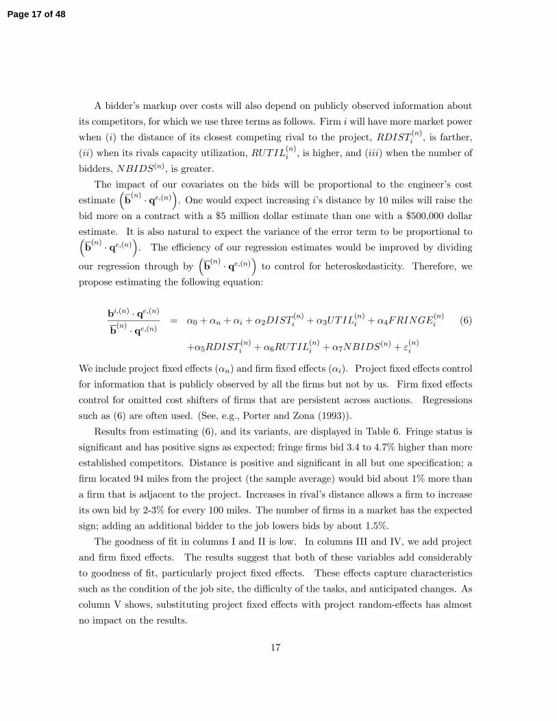
The impact of our covariates on the bids will be proportional to the engineer’s cost
estimate³b() · q()
´. One would expect increasing ’s distance by 10 miles will raise the
bid more on a contract with a $5 million dollar estimate than one with a $500,000 dollar
estimate. It is also natural to expect the variance of the error term to be proportional to³b() · q()
´. The efficiency of our regression estimates would be improved by dividing
our regression through by³b() · q()
´to control for heteroskedasticity. Therefore, we
propose estimating the following equation:
b() · q()b() · q()
= 0 + + + 2() + 3
() + 4
() (6)
+5() + 6
() + 7() +
()
We include project fixed effects () and firm fixed effects (). Project fixed effects control
for information that is publicly observed by all the firms but not by us. Firm fixed effects
control for omitted cost shifters of firms that are persistent across auctions. Regressions
such as (6) are often used. (See, e.g., Porter and Zona (1993)).
Results from estimating (6), and its variants, are displayed in Table 6. Fringe status is
significant and has positive signs as expected; fringe firms bid 3.4 to 4.7% higher than more
established competitors. Distance is positive and significant in all but one specification; a
firm located 94 miles from the project (the sample average) would bid about 1% more than
a firm that is adjacent to the project. Increases in rival’s distance allows a firm to increase
its own bid by 2-3% for every 100 miles. The number of firms in a market has the expected
sign; adding an additional bidder to the job lowers bids by about 1.5%.
The goodness of fit in columns I and II is low. In columns III and IV, we add project
and firm fixed effects. The results suggest that both of these variables add considerably
to goodness of fit, particularly project fixed effects. These effects capture characteristics
such as the condition of the job site, the difficulty of the tasks, and anticipated changes. As
column V shows, substituting project fixed effects with project random-effects has almost
no impact on the results.
17
Page 17 of 48
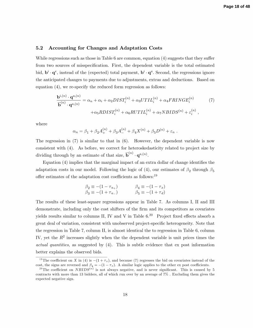
5.2 Accounting for Changes and Adaptation Costs
While regressions such as those in Table 6 are common, equation (4) suggests that they suffer
from two sources of misspecification. First, the dependent variable is the total estimated
bid, b · q instead of the (expected) total payment, b · q Second, the regressions ignorethe anticipated changes to payments due to adjustments, extras and deductions. Based on
equation (4), we re-specify the reduced form regression as follows:
b() · q()b() · q()
= + + 2() + 3
() + 4
() (7)
+5() + 6
() + 7() +
()
where
= 1 + 2()+ + 3
()− + 4
() + 5() +
The regression in (7) is similar to that in (6). However, the dependent variable is now
consistent with (4). As before, we correct for heteroskedasticity related to project size by
dividing through by an estimate of that size, b() · q().
Equation (4) implies that the marginal impact of an extra dollar of change identifies the
adaptation costs in our model. Following the logic of (4), our estimates of 2 through 5
offer estimates of the adaptation cost coefficients as follows:19
2 ≡ −(1− +) 4 ≡ −(1− )
3 ≡ −(1 + −) 5 ≡ −(1 + )
The results of these least-square regressions appear in Table 7. As columns I, II and III
demonstrate, including only the cost shifters of the firm and its competitors as covariates
yields results similar to columns II, IV and V in Table 6.20 Project fixed effects absorb a
great deal of variation, consistent with unobserved project-specific heterogeneity. Note that
the regression in Table 7, column II, is almost identical the to regression in Table 6, column
IV, yet the 2 increases slightly when the the dependent variable is unit prices times the
actual quantities, as suggested by (4). This is subtle evidence that ex post information
better explains the observed bids.
19The coefficient on in (4) is −(1 + ), and because (7) regresses the bid on covariates instead of the
cost, the signs are reversed and 4 = −(1− ). A similar logic applies to the other ex post coefficients.20The coefficient on () is not always negative, and is never significant. This is caused by 5
contracts with more than 13 bidders, all of which run over by an average of 7% . Excluding them gives the
expected negative sign.
18
Page 18 of 48
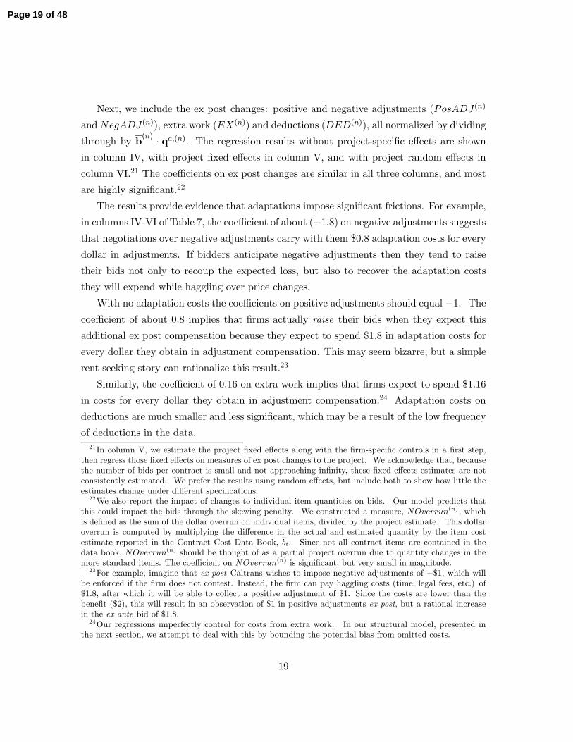
Next, we include the ex post changes: positive and negative adjustments (()
and()), extra work (()) and deductions (()), all normalized by dividing
through by b() · q(). The regression results without project-specific effects are shown
in column IV, with project fixed effects in column V, and with project random effects in
column VI.21 The coefficients on ex post changes are similar in all three columns, and most
are highly significant.22
The results provide evidence that adaptations impose significant frictions. For example,
in columns IV-VI of Table 7, the coefficient of about (−18) on negative adjustments suggeststhat negotiations over negative adjustments carry with them $08 adaptation costs for every
dollar in adjustments. If bidders anticipate negative adjustments then they tend to raise
their bids not only to recoup the expected loss, but also to recover the adaptation costs
they will expend while haggling over price changes.
With no adaptation costs the coefficients on positive adjustments should equal −1. Thecoefficient of about 08 implies that firms actually raise their bids when they expect this
additional ex post compensation because they expect to spend $18 in adaptation costs for
every dollar they obtain in adjustment compensation. This may seem bizarre, but a simple
rent-seeking story can rationalize this result.23
Similarly, the coefficient of 016 on extra work implies that firms expect to spend $116
in costs for every dollar they obtain in adjustment compensation.24 Adaptation costs on
deductions are much smaller and less significant, which may be a result of the low frequency
of deductions in the data.
21 In column V, we estimate the project fixed effects along with the firm-specific controls in a first step,
then regress those fixed effects on measures of ex post changes to the project. We acknowledge that, because
the number of bids per contract is small and not approaching infinity, these fixed effects estimates are not
consistently estimated. We prefer the results using random effects, but include both to show how little the
estimates change under different specifications.22We also report the impact of changes to individual item quantities on bids. Our model predicts that
this could impact the bids through the skewing penalty. We constructed a measure, () which
is defined as the sum of the dollar overrun on individual items, divided by the project estimate. This dollar
overrun is computed by multiplying the difference in the actual and estimated quantity by the item cost
estimate reported in the Contract Cost Data Book, . Since not all contract items are contained in the
data book, () should be thought of as a partial project overrun due to quantity changes in the
more standard items. The coefficient on () is significant, but very small in magnitude.23For example, imagine that ex post Caltrans wishes to impose negative adjustments of −$1, which will
be enforced if the firm does not contest. Instead, the firm can pay haggling costs (time, legal fees, etc.) of
$18, after which it will be able to collect a positive adjustment of $1. Since the costs are lower than the
benefit ($2), this will result in an observation of $1 in positive adjustments ex post, but a rational increase
in the ex ante bid of $1.8.24Our regressions imperfectly control for costs from extra work. In our structural model, presented in
the next section, we attempt to deal with this by bounding the potential bias from omitted costs.
19
Page 19 of 48
5.3 Endogenous Ex Post Changes and Omitted Costs
A concern with the analysis above is that ex post changes may be correlated with the error
term because of omitted costs that are observed by the bidders for which we cannot control.
For instance, a project in a more mountainous area will impose higher production costs and
will be more likely to require changes due to the more challenging terrain. If so, projects
with more changes have higher costs not because of adaptation costs but because of higher
production costs in rough terrains. Another plausible story is that very complex projects
impose serious delays and difficulties that increase the labor costs of production. If these
delays are the source of adjustments and deductions then the increased bids may actually
be a consequence of the increased production costs.
Recall that we observe the actual quantities used for each itemized component of the
contract, and have excellent cost data from the CCDB. If delays are accompanied by higher
costs of production, much of this will be captured by higher actual quantities of specified
contract items because these are controlled for by b() · q(), which in a simple univariate
regression explains 97.4% of the variation in the ex post bid. Hence, it seems safe to
believe that any omitted costs will be negligible. Nonetheless, we proceed to implement an
instrumental variable approach to correct for the possible endogeneity of ex post changes to
compensation by identifying an exogenous variable that affects ex post changes but does not
affect the unobserved project-specific production costs. In particular, we use the identity
of the Caltrans project engineer who supervised the project (i.e., the project manager) to
capture exogenous shocks to ex post changes.
While Caltrans highway contracts have numerous clauses devoted to changes, incomplete
contracts imply that project engineers have considerable discretion over the scope of changes
and deductions, and the process through which these changes are governed. It is well known
in the industry that there is considerable heterogeneity in the propensity of engineers to
make changes to the contract or impose deductions. Like in many fields, some engineers
are naturally adept at dealing with conflict and solving disputes while others are not. Some
engineers are harder to work with because of their propensity to impose deductions and
adjustments, causing disruptions to the efficient flow of work and imposing undesirable
renegotiation costs. Because every project is assigned to an engineer who handles several
projects, the identity of the engineer will shift the distribution of ex post changes to the
contracts he manages, independent of the specific project characteristics.
For the engineer’s identity to be a valid instrument it must be: (i) correlated with the
20
Page 20 of 48
endogenous variables (changes), and (ii) uncorrelated with the error term. Condition (i)
is fairly easy to verify. Our 819 contracts were handled by 334 unique engineers. After
dropping the 154 engineers who handle only one contract we are left with 180 engineers,
each managing at least 2 of the remaining 665 contracts.25 First-stage regressions of the
potentially endogenous ex post changes on dummy variables for these engineers confirm
instrument strength particularly for positive adjustments to compensation and overruns
on itemized contract elements, but suggest that they may be weak with regard to extra
work and deductions. See the online appendix for F-statistics and further details about
instrument quality.
Condition (ii) is not possible to verify directly since it is an identifying assumption, but
it is very plausible because of the way that contracts are assigned to engineers according to
the following sequence of events.26 The Caltrans engineering staff first draws the plans and
specifications for a given project. The project is then publicly advertised and the plans,
specifications and other bidding documents are made available to bidders. The location of
the project allows bidders to determine the district office from which the engineer will be
assigned. There are a handful of engineers at a given district office and they are matched to
projects based upon their expertise and availability. In most cases the engineer is assigned
early and noted on the project plans for bidders to contact prior to bidding with questions
about certain specifications. After bids are submitted and a winner is chosen, work begins
and changes to the project are made based upon work progress and site conditions.
Identification also requires that our instrument be mean-independent of the unobserved
costs () One might worry that project engineers predisposed to change the contract are
assigned in a nonrandom way to more or less complicated projects. We find, instead, that
the best predictor of the assignment of a project engineers to contracts is which of the
12 district offices the engineer works at: 96% of the engineers work in a single district.
However, district dummies alone do not predict ()+
()− () and (). All districts
have, on average, a similar share of projects that experience large changes. The scarce
supply of engineers in any given district, each with a limited capacity to take on projects,
25 In this set, the mean number of contracts per engineer is 3.69 with a standard deviation of 2.04. The
total value of projects managed by each engineer has a mean of $9.94 million and a standard deviation of
$13.6 million (using the engineer’s estimate). Our data consists of only asphalt contracts, while Caltrans
engineers also manage other contracts, hence the small number of contracts per engineer.26Any variable known at the time of bidding is a valid instrument (Hansen and Singleton (1982)) because
anything known at the time of bidding cannot be correlated with the forecast error of payoff relevant
variables.
21
Page 21 of 48
generates exogeneity in how engineers are assigned to projects with many changes.
Another test of random assignment is to regress measures of engineer experience on
ex post changes. We observe how many projects are assigned to a particular engineer,
which we interpret as a proxy for experience or productivity. We regress this variable on
()+
()− () and (). Nonrandom assignment implies that more experienced engineers
are assigned to projects with more changes. However, the 2 in this regression was less
than 0.01 and none of the coefficients on ex-post change variables were significant.
We present the instrumental variable estimates in columns VII, VIII and IX of Table 7.
In column VIII, as in column V, we regress the project level fixed effects on measures of ex
post changes to the project. Notice that the estimated values using our instruments are
similar to those from the OLS estimation in columns IV through VI. The estimated adap-
tation costs for adjustments are very similar in magnitude and significance, while those for
extra work and especially deductions are higher in magnitude. All are statistically signif-
icant in the fixed effects regression, and most are in the other two specifications (columns
VII and IX).
6 Structural Estimation
The reduced form analysis suggests that contractors build sizeable adaptation costs into
their bids in anticipation of ex post changes. However, much of the literature on contracting
has focused on other sources of distortion, primarily rents from private information and
market power, and, more recently, strategically skewed bidding. In order to assess the
relative magnitude of these distortions alongside those coming from adaptation costs, we
require a method for structurally estimating the model discussed in Section 3.
Our estimation approach builds on the two-step nonparametric estimators discussed in
Elyakime, Laffont, Loisel and Vuong (1994) and in Guerre, Perrigne, and Vuong (2000).
In the first step, we estimate the density and CDF of the bid distributions for project ,
denoted by () () and
() () respectively. In the second step, we estimate a particular
form of the penalty from skewed bidding and the adjustment cost coefficients, + −
and , by using the first order conditions in (4) to form a GMM estimator.
This approach also addresses some potential sources of misspecification in the reduced
form analysis.27 First, we note that since bidders will be uncertain about the magni-
27We acknowledge that our structural analysis may bring about other misspecifications, but our primary
goal is to assess the relative magnitude of sources of distortion.
22
Page 22 of 48
tude of ex post changes, the first order conditions should include the expected values of
(), (), () and () instead of their actual values. The stan-
dard econometric analysis of measurement error suggests that this will bias our reduced
form estimates of adaptation costs. Second, our reduced form regressions imperfectly ap-
proximate the first order conditions. For instance, we attempt to capture market power by
including () and
() as regressors. However, we can more precisely assess
market power by directly including the probability of winning, as implied by the first order
conditions (e.g. the right-hand side term in (5)).
Finally, we note that the structural model allows us to better flesh out the interpretation
of the error term, which is important for assessing the plausibility of the instruments used for
estimation. We propose instruments that allow for consistent estimation of the adaptation
costs when there are two sources of endogeneity. The first are the unobserved cost shocks
discussed in Section 4.3. The second are the expectational errors, mentioned above.
While the structural model uses different econometric methods, we shall find a great
deal of consistency with our reduced form results.
6.1 Estimating Bid Distributions
Since we wish to include measures of firm-specific distance and other controls for cross
firm heterogeneity, nonparametric approaches would suffer from a curse of dimensionality.28
Hence, we will estimate () () and
() () semiparametrically. We first run a regression
similar to those in Table 6:
b() · q()
b() · q
= ()0 + () +
()
where, as before, the dependent variable is the normalized estimated bid and () includes
the firm’s distance and whether or not it is a fringe firm.29 We also include an auction-
28Specifically, the sample size required in order to achieve the same level of precision in the estimates
increases dramatically as the number of covariates included in the kernel regression increases. See, for
example, Table 4.2 of Silverman (1986), as well as the Handbook of Econometrics chapter by Athey and
Haile (2007) and the references therein.29As shown later in equation (8) we are assuming that a bidder’s underlying private information about
costs have a multiplicative structure. That is, costs can be written as a product of b() · q and a bidder
specific private information shock. It follows from the linearity of expected utility and the definition of
Bayes-Nash equilibrium that if we divided all costs by b() · q and all bids by the same constant, this
transformed bid function is also an equilibrium. This idea is noted in both Athey and Haile (2007) section
6.1.1 and Haile, Hong and Shum (2003).
23
Page 23 of 48
specific random effect, () to control for project-specific characteristics that are observed
by the bidders but not the econometrician.30
Let b denote the estimated value of and let b() denote the fitted residual. We assume
that the residuals to this regression are iid with distribution (·). The iid assumption wouldbe satisfied if the noise on total costs had a multiplicative structure, which we describe in
detail in the next subsection. Under these assumptions, for project :
() () ≡ Pr
Ãb() · q()
b() · q()
≤
b() · q()
!= Pr
Ã()0 + () +
() ≤
b() · q()
!
≡
Ã
b() · q()
− ()0 − ()
!
That is, the distribution of the residuals, () can be used to derive the distribution of the
observed bids. We estimate using the distribution of the fitted residuals b() , and then
recover an estimate of () () by substituting in this distribution in place of An estimate
of () () can be formed using similar logic. We note that both
() () and
() () will be
estimated quite precisely because there are 3661 bids in our auction. Given the estimates
b() and b() we construct an estimate for
⎛⎝X 6=
() (b·q)1− ()
(b·q)
⎞⎠−1. Note that this term
accounts for varying numbers and identities of bidders across auctions. In particular, for
any given auction, let index the bidders, so that if the number or identity of bidders across
auctions changes, the set of firms indexed by will also change.
6.2 Estimating Adaptation Costs
As demonstrated in Section 5, the engineering cost estimate, b() · q(), is an excellent
predictor of the bids. Therefore, we assume that firm ’s cost is a variant of the engineer’s
cost estimate with the following multiplicative structure:
30As Krasnokutskaya (2011) has emphasized, failure to account for this form of unobserved heterogeneity
may lead to a considerable bias in the structural estimates. However, the strategies proposed in the lit-
erature for dealing with such heterogeneity, including Krasnokutskaya’s deconvolution-style estimator and
the parametric approach of Athey, Levin, and Seira (2011), are not straightforward to apply in our more
complicated framework. Instead, our use of random effects requires that the auction-specific effect () is
mean independent of the bidder’s private information, a restriction that is analogous to the independence
requirements of Krasnokutskaya’s more general deconvolution approach. As a robustness check we also es-
timated a version of the model with fixed effects and found little quantitative change in our results. We do
not rely upon these fixed effects results, however, because with a finite number of bidders per contract, we
have an incidental parameters problem and cannot consistently estimate the distribution of residuals.
24
Page 24 of 48
() = c
() · q() ≡ b() · q()(1 + e() ) (8)
That is, actual total costs for firm are a deviation from the engineer’s cost estimate
represented as a random variable e() times the engineering estimate b() · q(). The
assumption in (8) is similar to the multiplicative structure used in Krasnokutskaya (2011).
A similar assumption is also implicit in Hendricks, Pinkse and Porter (2003) where the
authors normalize lots by tract size. We assume that e() are iid.
By substituting (8) into the bidder’s first order condition (4), dividing by b() · q(),
explicitly writing out the various adaptations costs in , and rearranging terms we canwrite
()
b() · q()
=1
b() · q()
b() · q() − =1
()
()
6=
()
(b() · q())1−
()
(b() · q())
−1 (9)
+1
b() · q()
(1− +)
()+ + (1 + −)
()− + (1− )
()+ (1 + )
()
− 1
b() · q()
(b())− =1
()
(b())
6=
()
(b() · q())1−
()
(b() · q())
−1
To complete our structural model we also include two additional sources of error in
equation (9). The first source of error is that discussed in Section 4.3, the potential endo-
geneity of ex-post changes due to unobserved cost shocks. Recall that these omitted costs
are observed by the firms, but not already accounted for in our cost estimate b() · q().These costs may be correlated with
()+
()− () and () since projects with large ex
post changes are likely to be more complicated and more expensive to complete. We will
denote these additional unobserved costs as ()
The second source of error is an expectational error which results from bidders not
having perfect foresight about ()+
()− () and (). If risk neutral bidders have
rational expectations then the FOC should simply be modified to include ()+
()−
(), and (), the expected value of changes, instead of the actual values. In our
data, we do not directly observe bidders’ expectations. We therefore use well known
strategies akin to those applied in Euler Equation estimation in macroeconomics and finance
(described below) to estimate the model.31 We denote the expectational error as () ≡31This strategy is used in the seminal paper by Hansen and Singleton (1982). We only observe the realized
values of our variables and not a bidder’s expectation of those values. This creates a bias similar to an errors
in variables problem in linear regression. The idea in Hansen and Singleton is that information available
to the agent at the time of bidding can be used to construct a valid instrument since the difference between
25
Page 25 of 48
(1 − +)³()+ −
()+
´+ (1 + −)
³()− −
()−´+ (1 − )
¡() −()
¢+ (1 +
)(() −()).
Given these two additional sources of error, () and (), we can rewrite (9) as:
()
b() · q()
− ()
b() · q()
+()
b() · q()
= (10)
1
b() · q()
b() · q() − =1
()
()
6=
()
(b() · q())1−
()
(b() · q())
−1+
1
b() · q()
(1− +)
()+ + (1 + −)
()− + (1− )
()+ (1 + )
()
− 1
b() · q()
(b())− =1
()
(b())
6=
()
(b() · q())1−
()
(b() · q())
−1Equation (10) is identical to (9) except that we have brought over the two additional
sources of error to the left hand side. Taken together, we can define this composite errore() :
() ( + − ) ≡()
b() · q()
− ()
b() · q()
+()
b() · q()
Letting () denote the value of the instrument for bidder in auction we will use (10)
to form the moment condition below:
( + − ) =1
X
X
e() ( + − )(() −
() )
As in our reduced form analysis, we use engineer identities as our primary instruments
as they are uncorrelated with the unobserved cost shocks, (). They are also uncorrelated
with the expectational errors, by definition, because the engineer is typically known at the
time bidding occurs. We also include the engineer’s cost estimate as an instrument because
it is a natural shifter of the bidding strategies and thus, is correlated with the right hand side
variables in (10). We index the moment condition by to emphasize that the asymptotics
of our problem depend on the number of auctions in our sample growing large.
Let b and b denote a first stage estimate of the bid densities and distributions Let be a positive semi-definite weight matrix. We use the following GMM estimator:+ − = argmin ( + −
)0 ( + − )
the realized value of a random variable and its expected value must be orthogonal to current information.
If this were not the case, an agent could improve her estimate of the expected value by conditioning on this
instrument and hence would not be rational.
26
Page 26 of 48
The optimal weighting matrix can be calculated by using the inverse of the sample vari-
ance of (·) from a first step estimate which uses the identity weighting matrix. Newey
(1994) demonstrates that under suitable regularity conditions this estimator has normal as-
ymptotics despite depending on a nonparametric first stage. Furthermore, the asymptotic
variance surprisingly does not depend on how the nonparametric first stage is conducted,
as long as it is consistent. The first stage estimates of b and b are quite precise given our
regression coefficients (there are over 3600 individual bids). Therefore, it is quite unlikely
that our first stage bid density and distribution estimates introduce significant bias into the
estimates.
Lastly, we need to specify a particular functional form for the skewing penalty function
(b)We use a convenient special case of the conditions we imposed on (b) as follows,32
(b|b) =
X=1
¡ −
¢2 ¯ −
¯ (11)
We chose this specification because the penalty increases for bids that are further away
from the engineering estimate, and these get more weight when the actual quantity is
further away from the estimated one. While we could consider a more flexible penalty
function, the number of observations will limit the number of parameters we can include
in this term. This, together with our objective of keeping the structure of the model as
close to the standard literature as possible, is why we introduce this fairly parsimonious
specification.
6.3 Estimating Markups
Given the estimates¡bd+ d− bc¢, we can recover an estimate of the contractors’
implied markups. Using the functional form in (11) we estimate b, contractor ’s totalcost for installing the actual quantities by evaluating the empirical analogue of (4):
b() − c() · q() =
() − 2 () −
() −()
()
()
6=
()
(b() · q())1−
()
(b() · q())
−1
+
() −
2 () − ()
()
−(1−+)()
+ − (1 +−)()− − (1−)() − (1 +)()
32Strictly speaking, this does not guarantee that (b|b)
=0
is very large, but we still assume that an
interior solution exists. The estimates act as a reasonable reality check.
27
Page 27 of 48
Using our estimates of b, b, b,d+ d− c and b it is possible to evaluate the right handside of this equation.
6.4 Results
We summarize the structural estimates in Tables 8-11. Table 8 reports the parameter
values from our semiparametric GMM estimator. The adaptation cost estimates are similar
to the reduced form estimates discussed in Section 4. For instance, the last column of
Table 8 implies that every dollar of positive adjustment generates an additional $2.24 of
adaptation costs, while a negative adjustment generates an additional $2.69, though this
later estimate is not statistically significant. Recall that our results control for the quantities
that were actually installed by the contractor, b · q. Moreover, as we described in the
previous section, we have instrumented for the endogeneity of adjustments to account for a
possible bias from remaining omitted cost variables. Therefore, we argue that this estimate
reflects adaptation costs instead of omitted production costs (). It is worth noting that
our reduced form estimates from Table 7 Column IX were smaller, at $1.92 and $0.57 for
positive and negative adjustments respectively.
The other parameter estimates are also similar to the reduced form estimates. A dollar
of extra work generates up to $1.23 in adaptation costs, which almost matches the $1.21
estimated in the reduced form specification. Deductions are estimated to generate $1.61
in adaptation costs for every dollar of penalty assessed; however, the coefficient is not
statistically significant at standard levels. The lack of significance is most likely a result of
the small variation in this type of ex-post change. Deductions only affect 209 of the 819
contracts (compared to 752 contracts with extra work and 536 contracts with positive or
negative price adjustments), and much of the variance is driven by a single contract with a
particularly large deduction of almost $2.5 million.33
The estimated value of the skewing parameter, is -1.203E-05. Although the nega-
tive sign is inconsistent with the predictions of our theoretical model, this estimate is not
statistically significant at standard levels. It is also extremely small in monetary terms and
has no appreciable impact on profits or overall costs. The result that there are no large
penalties from skewing is quite robust to alternative specifications for the functional form of
33This contract was assessed $2.38 million in liquidated damages for completing the project 119 days late,
with the other deductions coming from quality and compliance penalties. Dropping this one contract does
not substantially affect the results.
28
Page 28 of 48
the skewing penalty. However, recall from Section 1 that positive and negative adjustments
are essentially due to renegotiating unit prices. As an empirical matter, it may be difficult
to separately identify a quadratic effect of overruns and underruns, as captured in from
the linear effect captured in + and − .
In Tables 9 and 10, we summarize our estimates of bidders’ markups. Our results
suggest that the industry is quite competitive. The median profit margin is 3.8 percent for
all bids and 12.1 percent for winning bids. We note that Granite Construction Inc., the
largest bidder in our data, is a publicly traded company and reported a net profit margin of
3.1 percent in 2005. The construction industry average according to Standard and Poors
is 1.9 percent. Profit margins based on SEC filings and our conception of profits differ in
many respects. However, the available direct evidence on profit margins suggests that the
construction industry is quite competitive and our results are consistent with this evidence.
As Table 9 demonstrates, markups over direct costs¡b − c¢·q are considerably higher
than the profit margin. This is because our analysis distinguished between the direct costs
of completing the project without adaptation costs and the added adaptation costs. The
median markup over direct costs,¡b − c¢ · q is $92,534 for all bids and $238,480 for
winning bids. The ratio of the markup over direct costs to the cost estimate for the median
job is 8.5 percent for all bids and 18 percent for winning bids. Contractors are effectively
extracting high margins on the components of the contract specified at the time of bidding,
in order to cover the costs of adapting to changes in the contract ex post.
In Table 10, we compare the estimates in Table 9 with the estimated markups found using
more standard methods that ignore the ex post changes to quantities and payments. Using
our first stage estimates of (b · q) and (b
· q), we evaluate the empirical analogueof equation (5), which is essentially the estimator discussed in Guerre, Perrigne and Vuong
(2000). Equation (5) is a special case of our model when we assume that q = q and
that that ex post changes can be excluded from the FOCs. Previous empirical structural
models of first price procurement auctions make these assumptions. Using this approach,
the median total markup is $161,277, or 12.2% of the estimate for winning bidders. These
results almost exactly match the median profit margins reported in the last two rows of
Table 9. By comparing the FOCs of the two models, this should not be surprising. The
only difference in the net profit margin under the two approaches comes from the skewing
penalty and the discrepancies between estimated and actual item quantities. Ex post
changes will shift the bid, changing what we refer to as the direct markup, but do not alter
29
Page 29 of 48
the contractors’ net profit margins. This is an important observation to the extent that it is a
consequence of the “pass through” of costs: the profit margins over total costs are practically
the same in both empirical models. However, our approach distinguishes the direct costs
from the adaptation costs that follow from incompletely specified contracts. Our results
therefore suggest that the standard FOC used in previous empirical studies is misspecified
because it does not account for ex post changes. In our application, failing to account for
contract adaptations leads to estimates with a very different economic interpretation, and
as discussed below, with very different policy implications.
Table 11 reports lower and upper bounds for the total adaptation costs estimated on
each project. These bounds are determined based on the possible margins that firms may
collect on extra work through change orders. Unlike adjustments and deductions, payments
made on extra work are not purely monetary transfers but are negotiated to cover costs of
additional work that cannot be fully accounted for in the itemized quantities listed in the
contract.34 Suppose that the contractor was able to earn a profit margin from renegotiating
these changes. As an upper bound, we can consider a case where contractors earn an
extra $1 in profits for every $1 of changes in scope, . Then the entire 123 would be
attributable to adaptation costs. Our upper bound for the total estimate of adaptations
costs would therefore be calculated as 2235++2689|−|+1233+160||. A much moreconservative approach would be to assume firms make zero margin on extra work, i.e. that
every $1 received ex post merely goes towards covering the costs of performance.35 Even in
this case, there remains an additional $0.23 that cannot be attributed to production costs,
and we instead attribute to the costs of adaptation. The lower bound is therefore calculated
as 2235+ + 2689|−|+ 0233 + 160||. The median estimate of adaptation costs is asizable component of costs by any standard. It has a lower bound of 4.0 (−01 85) percentof the engineer’s estimate and an upper bound of 8.8 (44 136) percent of that estimate.
34 Industry sources suggest that a twenty percent profit margin on change orders is most common. It is
helpful to recall that our cost estimate controls for the quantities actually installed and that positive and
negative adjustments are effectively changes to compensation from the unit prices. Hence, these are a pure
transfer and do not involve additional costs that we have not controlled for in our cost estimate.35This makes the reasonable assumption that firms do not negotiate ex post changes that result in them
losing money.
30
Page 30 of 48
7 Implications for Government Procurement
Our analysis offers some lessons for the design of procurement auctions. The first is that
the existing system does a good job of limiting rents and promoting competition. The
markup is modest, with the median bidder in our sample expecting a profit of 3.8% of the
estimate. More interesting, though, is how firms make their markup. Because adaptation
costs erode more than any positive gains from change orders, firms increase their bids ex
ante to extract high rents on prespecified project items. Among winning bidders the median
value of this direct markup, (b − c) · q is 17.7% of the project’s estimated costs.
Second, both the reduced form and structural estimates imply that adaptation costs
are substantial. The implied adaptation costs range from 60 cents to almost three dollars
for every dollar in change. These numbers might be surprising to economists who empha-
size private information and moral hazard as the main sources of inefficiency. However,
the results are consistent with current thinking in Construction and Engineering Project
Management. (See Bartholomew (1998), Clough and Sears (1994), Hinze (1993) and Sweet
(1994). Also see Bajari and Tadelis (2001) for a more complete set of references and dis-
cussion of the literature). One of the central concerns emphasized in this literature are
methods for minimizing the costs of disputes between contractors and buyers. The topic
of controlling contractor margins, by comparison, receives relatively little emphasis in this
literature.
The bounds on adaptation costs that were derived in Section 5.4 suggest that Caltrans
spent on average $318 million to $462 million on adaptation costs during our five and a
half year sample period. The average ratio of adaptation costs to the winning bid is 0.08 to
0.146. Even half of our lower bound would be substantial. An implication of competition
is that Caltrans, and hence the taxpayer, is ultimately responsible for expected adaptation
costs on the project as they are directly passed on from the bidders. Of course, we have no
way of estimating the direct adaptation costs born by Caltrans in the form of legal fees and
other haggling costs, which probably add significant costs. Since the source of these costs is
the incompleteness of project design and specifications, an obvious policy implication is to
consider increasing the ex ante costs and efforts put into estimating and specifying projects
before they are let out for bidding. Our analysis does not allow us to speculate on the costs
and benefits of adding more engineering efforts ex ante, and it would be impossible to avoid
contractual incompleteness and the implied agency problems altogether. However, since the
magnitude of adaptation costs is sizeable, there is room to consider some experimentation
31
Page 31 of 48

with more careful and costly design efforts, and to carefully examine the results of any such
added effort in ex ante engineering.
In related work, Bajari, McMillan and Tadelis (2009) study how private sector, non-
residential construction contracts are awarded in Northern California between 1995 and
2000. Unlike the public sector, private sector buyers can easily use mechanisms other than
competitive bidding to select a contractor. They find that open competitive bidding is
only used in 18 percent of the contracts and that 44 percent of the contracts are negotiated.
Also, negotiated contracts are more commonly used for projects that appear to be the most
complex for which ex post changes in plans and specifications are likely.
A perceived advantage of negotiated contracts is that they allow the architect, buyer
and contractor to discuss the project plans so that the contractor can point out pitfalls and
suggest modifications to the project design before work begins. Furthermore, negotiated
contracts are often based on cost plus compensation. As discussed in Bajari and Tadelis
(2001), the poor incentives to control costs that cost plus contracts provide are compensated
for by the ease in which renegotiating terms is achieved. When changes occur, the contractor
presents his receipts for the additional expenses and is reimbursed, thus avoiding the often
acrimonious process of negotiating change orders and reducing adaptation costs. The results
of this paper complement these previous papers by confirming that adaptation costs are
high in the construction industry, so that economizing on ex post adaptation costs is an
important potential source of cost savings. This may outweigh the benefits of competitive
bidding in selecting the lowest cost contractor, and providing the contractor with strong
incentives to lower production costs.
In the public sector, the use of negotiated contracts is problematic. Allowing for
greater discretion in contractor selection increases the possibility for favoritism, kick backs
and political corruption. The competitive bidding system is less prone to corruption since
it allows for free entry by qualified bidders and there is an objective criteria for selecting
the winning bidder. An important policy issue is whether it is possible to construct a
mechanism that balances ex post adaptation costs with the potential for corruption. To
the best of our knowledge, this question has not been explored in the existing theoretical
literature. Our research suggests that developing such a mechanism could dramatically
improve efficiency in public sector procurement.
32
Page 32 of 48
References
[1] Asker, John, and Estelle Cantillon. 2008 “Properties of Scoring Auctions.” RANDJournal of Economics, 39(1): 69-85.
[2] Athey, Susan, and Philip Haile. 2006. “Empirical Models of Auctions.” In Advances inEconomics and Econometrics, Theory and Applications: Ninth World Congress of theEconometric Society, Volume II, Ed. Richard Blundell, Whitney Newey, and TorstenPersson, 1-45. New York: Cambridge University Press.
[3] Athey, Susan, and Philip Haile. 2007. “Nonparametric Approaches to Auctions.” InHandbook of Econometrics, Vol. 6A, Ed. James Heckman and Edward Leamer. Ams-terdam: Elsevier.
[4] Athey, Susan, and Jonathan Levin. 2001 “Information and Competition in U.S. ForestService Timber Auctions.” Journal of Political Economy, 109(2): 375-417.
[5] Athey, Susan, Jonathan Levin, and Enrique Seira. 2011 “Comparing Open and SealedBid Auctions: Evidence from Timber Auctions.” Quarterly Journal of Economics,126(1): 207-257.
[6] Bajari, Patrick, Robert McMillan and Steven Tadelis. 2009 “Auctions versus Nego-tiations in Procurement: An Empirical Analysis.” Journal of Law, Economics, andOrganization, 25(2): 372-399.
[7] Bajari, Patrick, and Steven Tadelis. 2001 “Incentives Versus Transaction Costs: ATheory of Procurement Contracts.” RAND Journal of Economics, 32(3): 287-307.
[8] Bajari, Patrick, and Lixin Ye. 2003 “Deciding Between Competition and Collusion.”Review of Economics and Statistics, 85(4): 971-89.
[9] Bartholomew, Stuart H. 1998. Construction Contracting: Business and Legal Princi-ples. Upper Saddle River, NJ: Prentice-Hall, Inc.
[10] Chakravarty, Surajeet, and W. Bentley MacLeod. 2009 “Optimal Contracting in theShadow of the Law.” Rand Journal of Economics, 40(3): 533-557.
[11] Che, Yeon-Koo. 1993 “Design Competition through Multi-dimensional Auctions.”RAND Journal of Economics, 24(4): 668-80.
[12] Clough, Richard H., and Glenn A. Sears. 1994. Construction Contracting, 6th ed. NewYork: Wiley.
[13] Crocker, Keith J., and Kenneth J. Reynolds. 1993. “The Efficiency of Incomplete Con-tracts: An Empirical Analysis of Air Force Engine Procurement.” RAND Journal ofEconomics, 24(1): 126-46.
[14] Elyakime, Bernard, Jean-Jacques Laffont, Patrice Loisel, and Quang Vuong. 1994.“First-Price Sealed-Bid Auctions with Secret Reservation Prices.” Annales D’Economieet de Statistique, 34(1): 115—41.
[15] Guerre, Emmanuel, Isabelle Perrigne, and Quang Vuong. 2000. “Optimal Nonparamet-ric Estimation of First—Price Auctions.” Econometrica, 68(3): 525-74.
33
Page 33 of 48
[16] Haile, Philip. 2001. “Auctions with Resale Markets: An Application to U.S. ForestService Timber Sales.” American Economic Review, 92(3): 399-427.
[17] Haile, P., H. Hong and M. Shum (2003), “Nonparametric Tests for Common Values inFirst-Price Sealed-Bid Auctions,” NBER Working Paper 10105.
[18] Hanna, Awad S., and Murat Gunduz. 2004. “Impact of Change Orders on Small Labor-Intensive Projects.” Journal of Construction Engineering and Management, 130(5):726-733.
[19] Hansen, Lars P., and Kenneth J. Singleton. 1982. “Generalized Instrumental VariablesEstimation of Nonlinear Rational Expectations Models.” Econometrica, 50(5): 1269-1286.
[20] Hendricks, Kenneth, Joris Pinkse, and Robert H. Porter. 2003. “Empirical Implicationsof Equilibrium Bidding in First-Price, Symmetric, Common-Value Auctions.” Reviewof Economic Studies, 70: 115-46.
[21] Hinze, Jim. 1993. Construction Contracts, McGraw-Hill Series in Construction Engi-neering and Project Management. Boston: Irwin/McGraw-Hill.
[22] Hubbard, Timothy P., Tong Li, and Harry J. Paarsch. Forthcoming. “SemiparametricEstimation in Models of First-Price, Sealed-Bid Auctions with Affiliation,” Journal ofEconometrics.
[23] Krasnokutskaya, Elena. 2011. “Identification and Estimation in Highway Procure-ment Auctions under Unobserved Auction Heterogeneity.” Review of Economic Studies,78(1): 293-327.
[24] Krasnokutskaya, Elena, and Katja Seim. Forthcoming. “Bid Preference Programs andParticipation in Procurement.” American Economic Review.
[25] Lebrun, Bernard 2006. “Uniqueness of the equilibrium in first-price auctions.” Gamesand Economic Behavior 55(1):131—151
[26] Newey, Whitney K. 1994. “The Asymptotic Variance of Semiparametric Estimators.”Econometrica, 62(6): 1349-82.
[27] Paarsch, Harry J. 1992. “Deciding between the Common and Private Value Paradigmsin Empirical Models of Auctions.” Journal of Econometrics, 51(1): 191-215.
[28] Pesendorfer, Martin, and Mireia Jofre-Bonet. 2003. “Estimation of a Dynamic AuctionGame.” Econometrica, 71(5): 1443-89.
[29] Porter, Robert H., and J. Douglas Zona. 1993. “Detection of Bid Rigging in Procure-ment Auctions.” Journal of Political Economy, 101(3): 518-38.
[30] Silverman, Bernard W. 1986. Density Analysis for Statistics and Data Analysis. Lon-don: Chapman and Hall.
[31] Sweet, Justin. 1994. Legal Aspects of Architecture, Engineering and the ConstructionProcess, 5th ed. Minneapolis-St. Paul, MN: West Publishing Company.
[32] Williamson, Oliver E. 1971. “The Vertical Integration of Production: Market FailureConsiderations.” American Economic Review, 63(2): 316-25.
34
Page 34 of 48
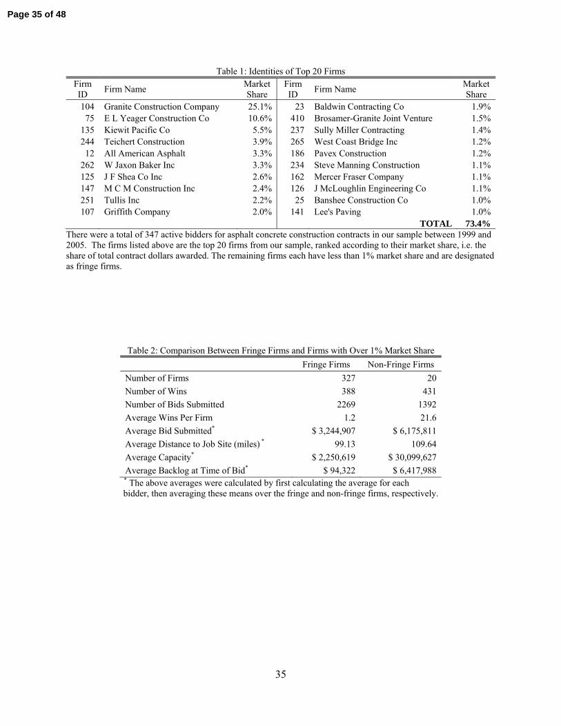
35
Table 1: Identities of Top 20 Firms Firm ID
Firm Name Market Share
Firm ID
Firm Name Market Share
104 Granite Construction Company 25.1% 23 Baldwin Contracting Co 1.9% 75 E L Yeager Construction Co 10.6% 410 Brosamer-Granite Joint Venture 1.5%
135 Kiewit Pacific Co 5.5% 237 Sully Miller Contracting 1.4% 244 Teichert Construction 3.9% 265 West Coast Bridge Inc 1.2% 12 All American Asphalt 3.3% 186 Pavex Construction 1.2%
262 W Jaxon Baker Inc 3.3% 234 Steve Manning Construction 1.1% 125 J F Shea Co Inc 2.6% 162 Mercer Fraser Company 1.1% 147 M C M Construction Inc 2.4% 126 J McLoughlin Engineering Co 1.1% 251 Tullis Inc 2.2% 25 Banshee Construction Co 1.0% 107 Griffith Company 2.0% 141 Lee's Paving 1.0%
TOTAL 73.4% There were a total of 347 active bidders for asphalt concrete construction contracts in our sample between 1999 and 2005. The firms listed above are the top 20 firms from our sample, ranked according to their market share, i.e. the share of total contract dollars awarded. The remaining firms each have less than 1% market share and are designated as fringe firms.
Table 2: Comparison Between Fringe Firms and Firms with Over 1% Market Share
Fringe Firms Non-Fringe Firms
Number of Firms 327 20
Number of Wins 388 431
Number of Bids Submitted 2269 1392
Average Wins Per Firm 1.2 21.6
Average Bid Submitted* $ 3,244,907 $ 6,175,811
Average Distance to Job Site (miles) * 99.13 109.64
Average Capacity* $ 2,250,619 $ 30,099,627
Average Backlog at Time of Bid* $ 94,322 $ 6,417,988 * The above averages were calculated by first calculating the average for each bidder, then averaging these means over the fringe and non-fringe firms, respectively.
Page 35 of 48
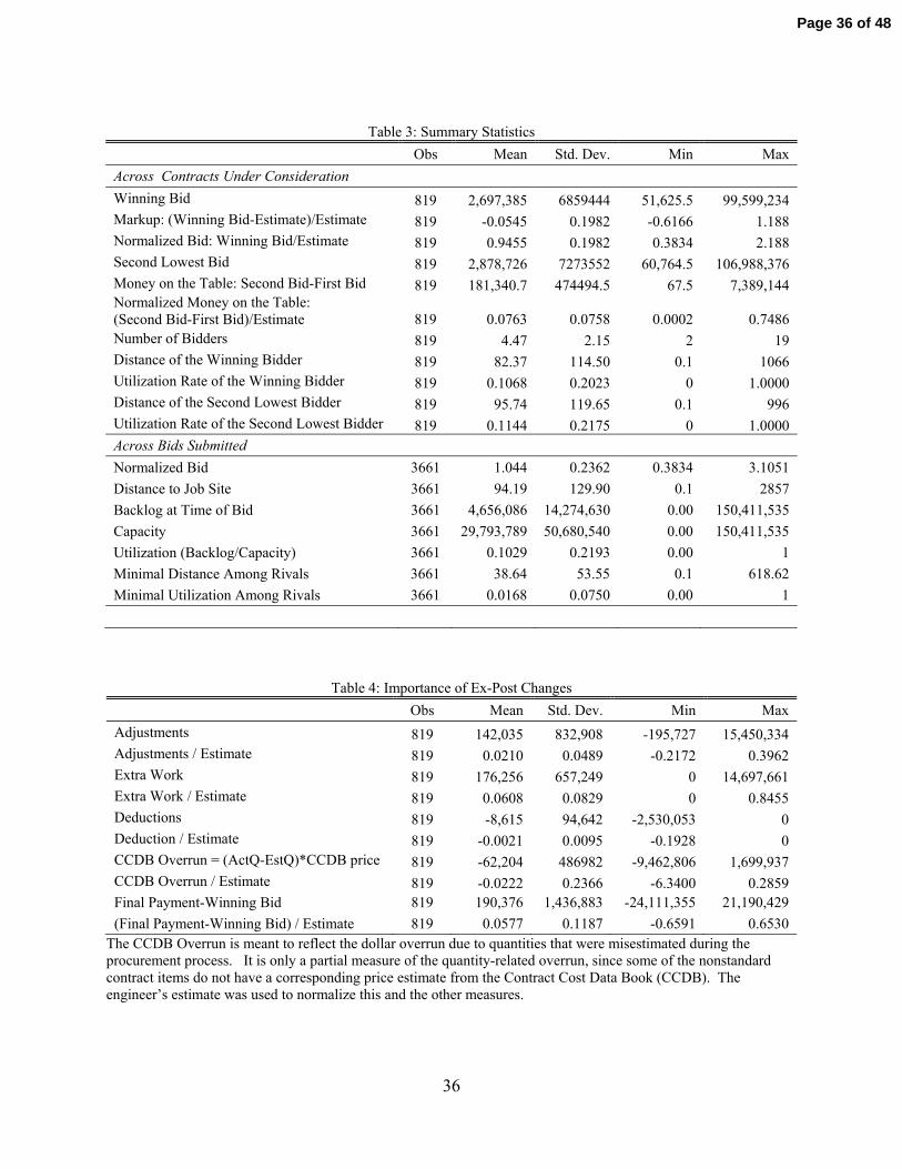
36
Table 3: Summary Statistics
Obs Mean Std. Dev. Min Max
Across Contracts Under Consideration
Winning Bid 819 2,697,385 6859444 51,625.5 99,599,234 Markup: (Winning Bid-Estimate)/Estimate 819 -0.0545 0.1982 -0.6166 1.188 Normalized Bid: Winning Bid/Estimate 819 0.9455 0.1982 0.3834 2.188 Second Lowest Bid 819 2,878,726 7273552 60,764.5 106,988,376 Money on the Table: Second Bid-First Bid 819 181,340.7 474494.5 67.5 7,389,144 Normalized Money on the Table: (Second Bid-First Bid)/Estimate 819 0.0763 0.0758 0.0002 0.7486 Number of Bidders 819 4.47 2.15 2 19 Distance of the Winning Bidder 819 82.37 114.50 0.1 1066 Utilization Rate of the Winning Bidder 819 0.1068 0.2023 0 1.0000 Distance of the Second Lowest Bidder 819 95.74 119.65 0.1 996 Utilization Rate of the Second Lowest Bidder 819 0.1144 0.2175 0 1.0000 Across Bids Submitted
Normalized Bid 3661 1.044 0.2362 0.3834 3.1051
Distance to Job Site 3661 94.19 129.90 0.1 2857
Backlog at Time of Bid 3661 4,656,086 14,274,630 0.00 150,411,535
Capacity 3661 29,793,789 50,680,540 0.00 150,411,535
Utilization (Backlog/Capacity) 3661 0.1029 0.2193 0.00 1
Minimal Distance Among Rivals 3661 38.64 53.55 0.1 618.62
Minimal Utilization Among Rivals 3661 0.0168 0.0750 0.00 1
Table 4: Importance of Ex-Post Changes
Obs Mean Std. Dev. Min Max
Adjustments 819 142,035 832,908 -195,727 15,450,334 Adjustments / Estimate 819 0.0210 0.0489 -0.2172 0.3962 Extra Work 819 176,256 657,249 0 14,697,661 Extra Work / Estimate 819 0.0608 0.0829 0 0.8455 Deductions 819 -8,615 94,642 -2,530,053 0 Deduction / Estimate 819 -0.0021 0.0095 -0.1928 0 CCDB Overrun = (ActQ-EstQ)*CCDB price 819 -62,204 486982 -9,462,806 1,699,937 CCDB Overrun / Estimate 819 -0.0222 0.2366 -6.3400 0.2859 Final Payment-Winning Bid 819 190,376 1,436,883 -24,111,355 21,190,429
(Final Payment-Winning Bid) / Estimate 819 0.0577 0.1187 -0.6591 0.6530 The CCDB Overrun is meant to reflect the dollar overrun due to quantities that were misestimated during the procurement process. It is only a partial measure of the quantity-related overrun, since some of the nonstandard contract items do not have a corresponding price estimate from the Contract Cost Data Book (CCDB). The engineer’s estimate was used to normalize this and the other measures.
Page 36 of 48
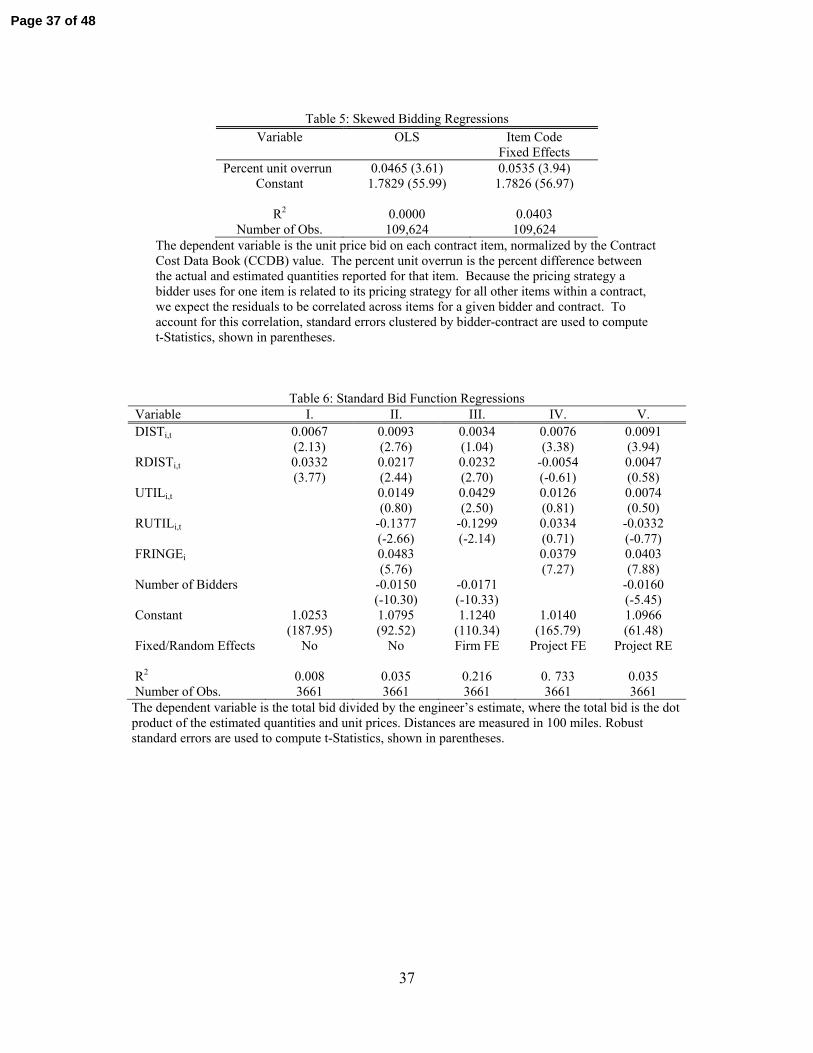
37
Table 5: Skewed Bidding Regressions
Variable OLS Item Code Fixed Effects
Percent unit overrun 0.0465 (3.61) 0.0535 (3.94) Constant 1.7829 (55.99) 1.7826 (56.97)
R2 0.0000 0.0403
Number of Obs. 109,624 109,624 The dependent variable is the unit price bid on each contract item, normalized by the Contract Cost Data Book (CCDB) value. The percent unit overrun is the percent difference between the actual and estimated quantities reported for that item. Because the pricing strategy a bidder uses for one item is related to its pricing strategy for all other items within a contract, we expect the residuals to be correlated across items for a given bidder and contract. To account for this correlation, standard errors clustered by bidder-contract are used to compute t-Statistics, shown in parentheses.
Table 6: Standard Bid Function Regressions Variable I. II. III. IV. V. DISTi,t 0.0067
(2.13) 0.0093 (2.76)
0.0034 (1.04)
0.0076 (3.38)
0.0091 (3.94)
RDISTi,t 0.0332 (3.77)
0.0217 (2.44)
0.0232 (2.70)
-0.0054 (-0.61)
0.0047 (0.58)
UTILi,t
0.0149 (0.80)
0.0429 (2.50)
0.0126 (0.81)
0.0074 (0.50)
RUTILi,t
-0.1377 (-2.66)
-0.1299 (-2.14)
0.0334 (0.71)
-0.0332 (-0.77)
FRINGEi
0.0483 (5.76)
0.0379 (7.27)
0.0403 (7.88)
Number of Bidders
-0.0150 (-10.30)
-0.0171 (-10.33)
-0.0160 (-5.45)
Constant 1.0253 (187.95)
1.0795 (92.52)
1.1240 (110.34)
1.0140 (165.79)
1.0966 (61.48)
Fixed/Random Effects No No Firm FE Project FE Project RE R2 0.008 0.035 0.216 0. 733 0.035 Number of Obs. 3661 3661 3661 3661 3661
The dependent variable is the total bid divided by the engineer’s estimate, where the total bid is the dot product of the estimated quantities and unit prices. Distances are measured in 100 miles. Robust standard errors are used to compute t-Statistics, shown in parentheses.
Page 37 of 48
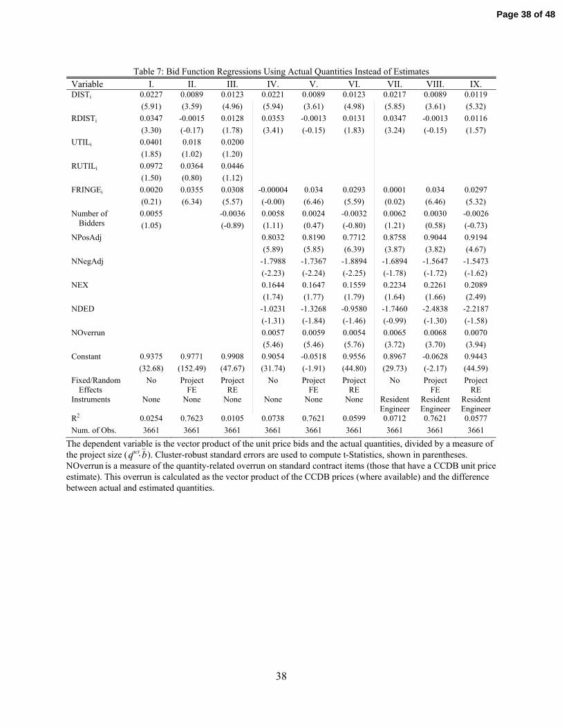
38
Table 7: Bid Function Regressions Using Actual Quantities Instead of Estimates Variable I. II. III. IV. V. VI. VII. VIII. IX. DISTi 0.0227 0.0089 0.0123 0.0221 0.0089 0.0123 0.0217 0.0089 0.0119
(5.91) (3.59) (4.96) (5.94) (3.61) (4.98) (5.85) (3.61) (5.32)
RDISTi 0.0347 -0.0015 0.0128 0.0353 -0.0013 0.0131 0.0347 -0.0013 0.0116
(3.30) (-0.17) (1.78) (3.41) (-0.15) (1.83) (3.24) (-0.15) (1.57)
UTILi 0.0401 0.018 0.0200
(1.85) (1.02) (1.20)
RUTILi 0.0972 0.0364 0.0446
(1.50) (0.80) (1.12)
FRINGEi 0.0020 0.0355 0.0308 -0.00004 0.034 0.0293 0.0001 0.034 0.0297
(0.21) (6.34) (5.57) (-0.00) (6.46) (5.59) (0.02) (6.46) (5.32)
Number of Bidders
0.0055 -0.0036 0.0058 0.0024 -0.0032 0.0062 0.0030 -0.0026
(1.05) (-0.89) (1.11) (0.47) (-0.80) (1.21) (0.58) (-0.73)
NPosAdj 0.8032 0.8190 0.7712 0.8758 0.9044 0.9194
(5.89) (5.85) (6.39) (3.87) (3.82) (4.67)
NNegAdj -1.7988 -1.7367 -1.8894 -1.6894 -1.5647 -1.5473
(-2.23) (-2.24) (-2.25) (-1.78) (-1.72) (-1.62)
NEX 0.1644 0.1647 0.1559 0.2234 0.2261 0.2089
(1.74) (1.77) (1.79) (1.64) (1.66) (2.49)
NDED -1.0231 -1.3268 -0.9580 -1.7460 -2.4838 -2.2187
(-1.31) (-1.84) (-1.46) (-0.99) (-1.30) (-1.58)
NOverrun 0.0057 0.0059 0.0054 0.0065 0.0068 0.0070
(5.46) (5.46) (5.76) (3.72) (3.70) (3.94)
Constant 0.9375 0.9771 0.9908 0.9054 -0.0518 0.9556 0.8967 -0.0628 0.9443
(32.68) (152.49) (47.67) (31.74) (-1.91) (44.80) (29.73) (-2.17) (44.59)
Fixed/Random Effects
No Project FE
Project RE
No Project FE
Project RE
No Project FE
Project RE
Instruments None None None None None None Resident Engineer
Resident Engineer
Resident Engineer
R2 0.0254 0.7623 0.0105 0.0738 0.7621 0.0599 0.0712 0.7621 0.0577
Num. of Obs. 3661 3661 3661 3661 3661 3661 3661 3661 3661
The dependent variable is the vector product of the unit price bids and the actual quantities, divided by a measure of the project size ( bqact ). Cluster-robust standard errors are used to compute t-Statistics, shown in parentheses. NOverrun is a measure of the quantity-related overrun on standard contract items (those that have a CCDB unit price estimate). This overrun is calculated as the vector product of the CCDB prices (where available) and the difference between actual and estimated quantities.
Page 38 of 48
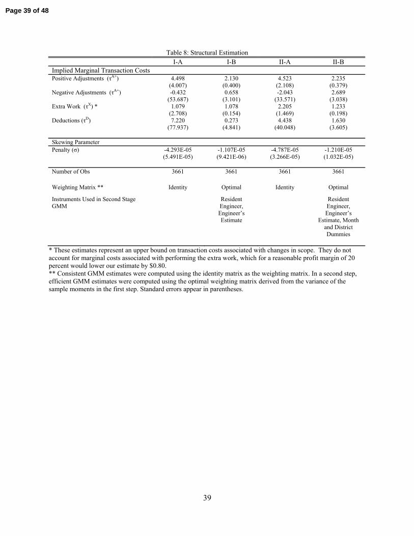
39
Table 8: Structural Estimation I-A I-B II-A II-B Implied Marginal Transaction Costs Positive Adjustments (τA+) 4.498 2.130 4.523 2.235
(4.007) (0.400) (2.108) (0.379) Negative Adjustments (τA+) -0.432 0.658 -2.043 2.689
(53.687) (3.101) (33.571) (3.038) Extra Work (τX) * 1.079 1.078 2.205 1.233
(2.708) (0.154) (1.469) (0.198) Deductions (τD) 7.220 0.273 4.438 1.630
(77.937) (4.841) (40.048) (3.605) Skewing Parameter Penalty (σ) -4.293E-05 -1.107E-05 -4.787E-05 -1.210E-05 (5.491E-05) (9.421E-06) (3.266E-05) (1.032E-05)
Number of Obs 3661 3661 3661 3661
Weighting Matrix ** Identity Optimal Identity Optimal
Instruments Used in Second Stage GMM
Resident Engineer, Engineer’s Estimate
Resident Engineer, Engineer’s
Estimate, Month and District Dummies
* These estimates represent an upper bound on transaction costs associated with changes in scope. They do not account for marginal costs associated with performing the extra work, which for a reasonable profit margin of 20 percent would lower our estimate by $0.80. ** Consistent GMM estimates were computed using the identity matrix as the weighting matrix. In a second step, efficient GMM estimates were computed using the optimal weighting matrix derived from the variance of the sample moments in the first step. Standard errors appear in parentheses.
Page 39 of 48
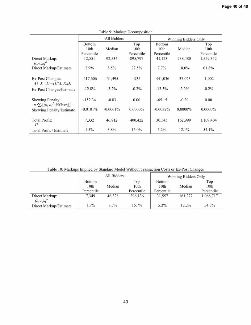
40
Table 9: Markup Decomposition
All Bidders Winning Bidders Only
Bottom
10th Percentile
Median
Top 10th
Percentile
Bottom 10th
Percentile
Median
Top 10th
Percentile Direct Markup: (bi-ci)q
a 12,551 92,534 895,797 41,123 238,480 1,559,352
Direct Markup/Estimate 2.9% 8.5% 27.5% 7.7% 18.0% 61.8%
Ex-Post Changes: A+ X +D –TC(A, X,D)
-417,606 -31,495 -935 -441,036 -37,023 -1,002
Ex-Post Changes/Estimate -12.8% -3.2% -0.2% -13.5% -3.3% -0.2%
Skewing Penalty: σ ·∑t [(bi-b)2 |%Overt|]
-152.34 -0.83 0.00 -65.15 -0.29 0.00
Skewing Penalty/Estimate -0.0101% -0.0001% 0.0000% -0.0032% 0.0000% 0.0000%
Total Profit: Π
7,332 46,812 400,422 30,545 162,999 1,109,404
Total Profit / Estimate 1.5% 3.8% 16.0% 5.2% 12.1% 54.1%
Table 10: Markups Implied by Standard Model Without Transaction Costs or Ex-Post Changes
All Bidders Winning Bidders Only
Bottom
10th Percentile
Median
Top 10th
Percentile
Bottom 10th
Percentile
Median
Top 10th
Percentile Direct Markup: (bi-ci)q
a 7,349 46,328 396,136 31,557 161,277 1,068,717
Direct Markup/Estimate 1.5% 3.7% 15.7% 5.2% 12.2% 54.5%
Page 40 of 48
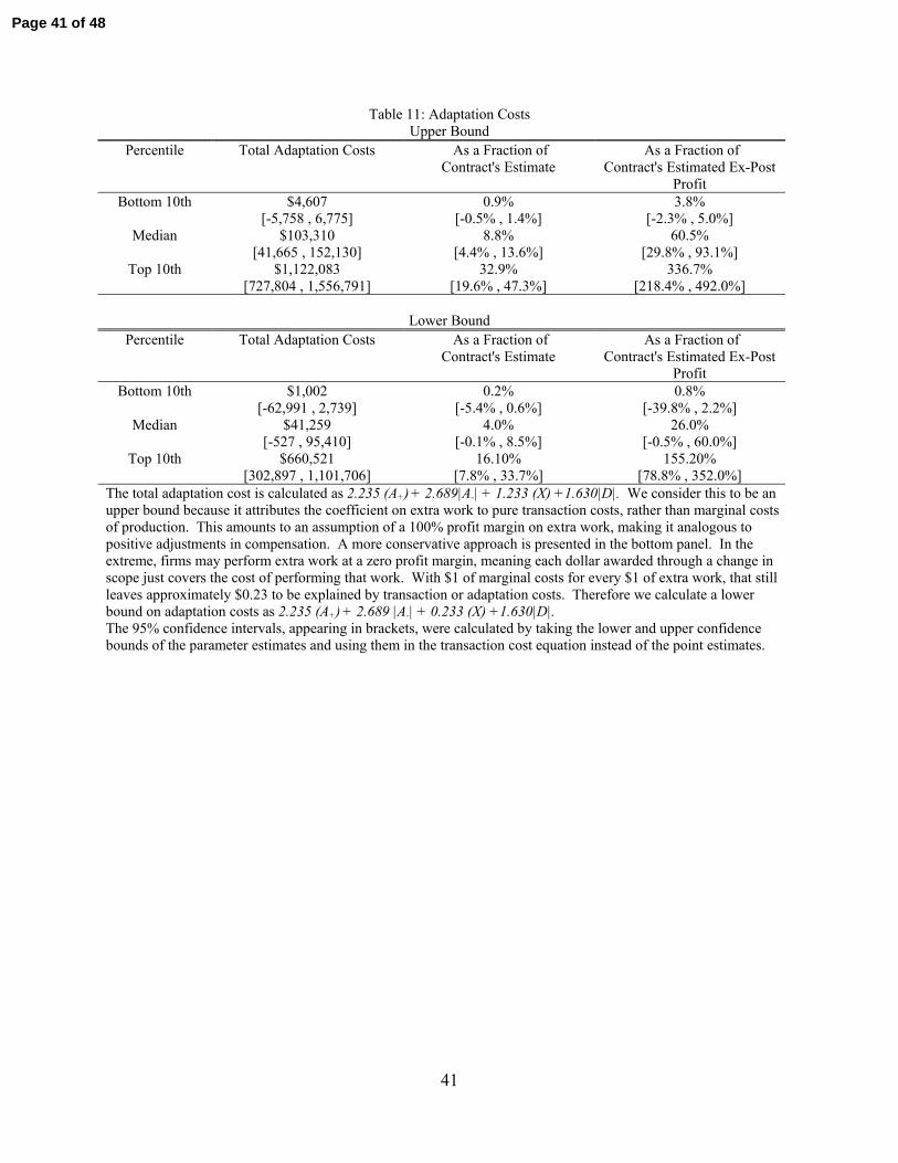
41
Table 11: Adaptation Costs Upper Bound
Percentile Total Adaptation Costs As a Fraction of Contract's Estimate
As a Fraction of Contract's Estimated Ex-Post
Profit Bottom 10th $4,607 0.9% 3.8%
[-5,758 , 6,775] [-0.5% , 1.4%] [-2.3% , 5.0%] Median $103,310 8.8% 60.5%
[41,665 , 152,130] [4.4% , 13.6%] [29.8% , 93.1%] Top 10th $1,122,083 32.9% 336.7%
[727,804 , 1,556,791] [19.6% , 47.3%] [218.4% , 492.0%]
Lower Bound Percentile Total Adaptation Costs As a Fraction of
Contract's Estimate As a Fraction of
Contract's Estimated Ex-Post Profit
Bottom 10th $1,002 0.2% 0.8% [-62,991 , 2,739] [-5.4% , 0.6%] [-39.8% , 2.2%]
Median $41,259 4.0% 26.0% [-527 , 95,410] [-0.1% , 8.5%] [-0.5% , 60.0%]
Top 10th $660,521 16.10% 155.20% [302,897 , 1,101,706] [7.8% , 33.7%] [78.8% , 352.0%]
The total adaptation cost is calculated as 2.235 (A+) + 2.689|A-| + 1.233 (X) +1.630|D|. We consider this to be an upper bound because it attributes the coefficient on extra work to pure transaction costs, rather than marginal costs of production. This amounts to an assumption of a 100% profit margin on extra work, making it analogous to positive adjustments in compensation. A more conservative approach is presented in the bottom panel. In the extreme, firms may perform extra work at a zero profit margin, meaning each dollar awarded through a change in scope just covers the cost of performing that work. With $1 of marginal costs for every $1 of extra work, that still leaves approximately $0.23 to be explained by transaction or adaptation costs. Therefore we calculate a lower bound on adaptation costs as 2.235 (A+) + 2.689 |A-| + 0.233 (X) +1.630|D|. The 95% confidence intervals, appearing in brackets, were calculated by taking the lower and upper confidence bounds of the parameter estimates and using them in the transaction cost equation instead of the point estimates.
Page 41 of 48
Online Appendix for
Bidding for Incomplete Contracts:An Empirical Analysis of Adaptation Costs
Patrick Bajari∗ Stephanie Houghton † Steven Tadelis‡
March 2012
The following Appendix provides additional details about the data and estimation pro-
cedures used in the paper. Tables A1-A3 summarize the bidding behavior of the top 20
firms in our sample, the number of participants in each auction, and the distribution of
these auctions over time. The next two tables present information about our use of in-
struments in the reduced form regressions of bids on contract characteristics and ex post
changes. Specifically, in Table A4, we present F-statistics from first-stage regressions
of the instruments. Table A5 demonstrates the robustness of our results by comparing
model specifications which instrument for different subsets of the potentially endogenous
variables. In Table A6, we present results from the structural model in which we control
for unobserved auction heterogeneity using fixed effects in the first-stage recovery of the
bid distribution. A final section describes in detail the procedure used to obtain these
structural estimates.
∗University of Minnesota and NBER†Texas A&M University‡UC Berkeley
Page 42 of 48
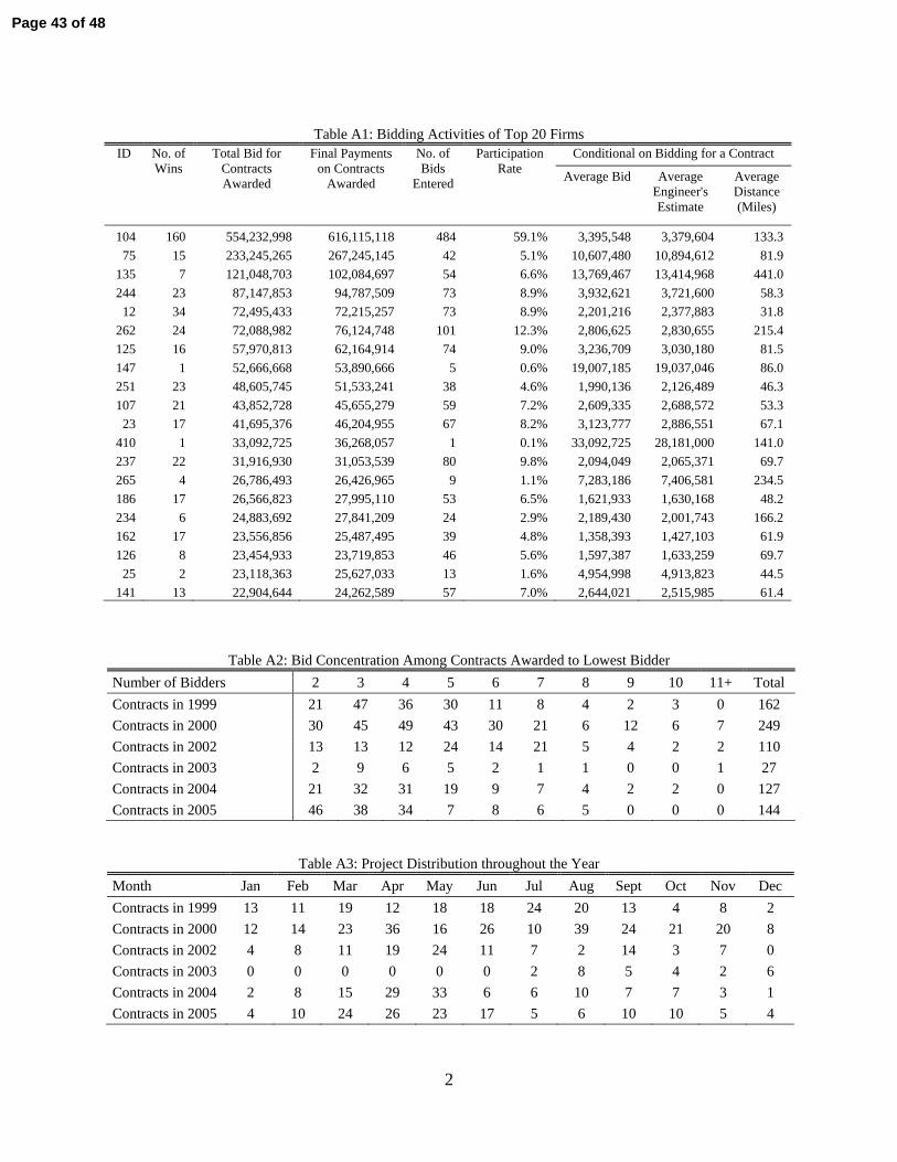
2
Table A1: Bidding Activities of Top 20 Firms
ID No. of Wins
Total Bid for Contracts Awarded
Final Payments on Contracts
Awarded
No. of Bids
Entered
Participation Rate
Conditional on Bidding for a Contract
Average Bid Average Engineer's Estimate
Average Distance (Miles)
104 160 554,232,998 616,115,118 484 59.1% 3,395,548 3,379,604 133.3
75 15 233,245,265 267,245,145 42 5.1% 10,607,480 10,894,612 81.9
135 7 121,048,703 102,084,697 54 6.6% 13,769,467 13,414,968 441.0
244 23 87,147,853 94,787,509 73 8.9% 3,932,621 3,721,600 58.3
12 34 72,495,433 72,215,257 73 8.9% 2,201,216 2,377,883 31.8
262 24 72,088,982 76,124,748 101 12.3% 2,806,625 2,830,655 215.4
125 16 57,970,813 62,164,914 74 9.0% 3,236,709 3,030,180 81.5
147 1 52,666,668 53,890,666 5 0.6% 19,007,185 19,037,046 86.0
251 23 48,605,745 51,533,241 38 4.6% 1,990,136 2,126,489 46.3
107 21 43,852,728 45,655,279 59 7.2% 2,609,335 2,688,572 53.3
23 17 41,695,376 46,204,955 67 8.2% 3,123,777 2,886,551 67.1
410 1 33,092,725 36,268,057 1 0.1% 33,092,725 28,181,000 141.0
237 22 31,916,930 31,053,539 80 9.8% 2,094,049 2,065,371 69.7
265 4 26,786,493 26,426,965 9 1.1% 7,283,186 7,406,581 234.5
186 17 26,566,823 27,995,110 53 6.5% 1,621,933 1,630,168 48.2
234 6 24,883,692 27,841,209 24 2.9% 2,189,430 2,001,743 166.2
162 17 23,556,856 25,487,495 39 4.8% 1,358,393 1,427,103 61.9
126 8 23,454,933 23,719,853 46 5.6% 1,597,387 1,633,259 69.7
25 2 23,118,363 25,627,033 13 1.6% 4,954,998 4,913,823 44.5
141 13 22,904,644 24,262,589 57 7.0% 2,644,021 2,515,985 61.4
Table A2: Bid Concentration Among Contracts Awarded to Lowest Bidder
Number of Bidders 2 3 4 5 6 7 8 9 10 11+ Total
Contracts in 1999 21 47 36 30 11 8 4 2 3 0 162
Contracts in 2000 30 45 49 43 30 21 6 12 6 7 249
Contracts in 2002 13 13 12 24 14 21 5 4 2 2 110
Contracts in 2003 2 9 6 5 2 1 1 0 0 1 27
Contracts in 2004 21 32 31 19 9 7 4 2 2 0 127
Contracts in 2005 46 38 34 7 8 6 5 0 0 0 144
Table A3: Project Distribution throughout the Year
Month Jan Feb Mar Apr May Jun Jul Aug Sept Oct Nov Dec
Contracts in 1999 13 11 19 12 18 18 24 20 13 4 8 2
Contracts in 2000 12 14 23 36 16 26 10 39 24 21 20 8
Contracts in 2002 4 8 11 19 24 11 7 2 14 3 7 0
Contracts in 2003 0 0 0 0 0 0 2 8 5 4 2 6
Contracts in 2004 2 8 15 29 33 6 6 10 7 7 3 1
Contracts in 2005 4 10 24 26 23 17 5 6 10 10 5 4
Page 43 of 48
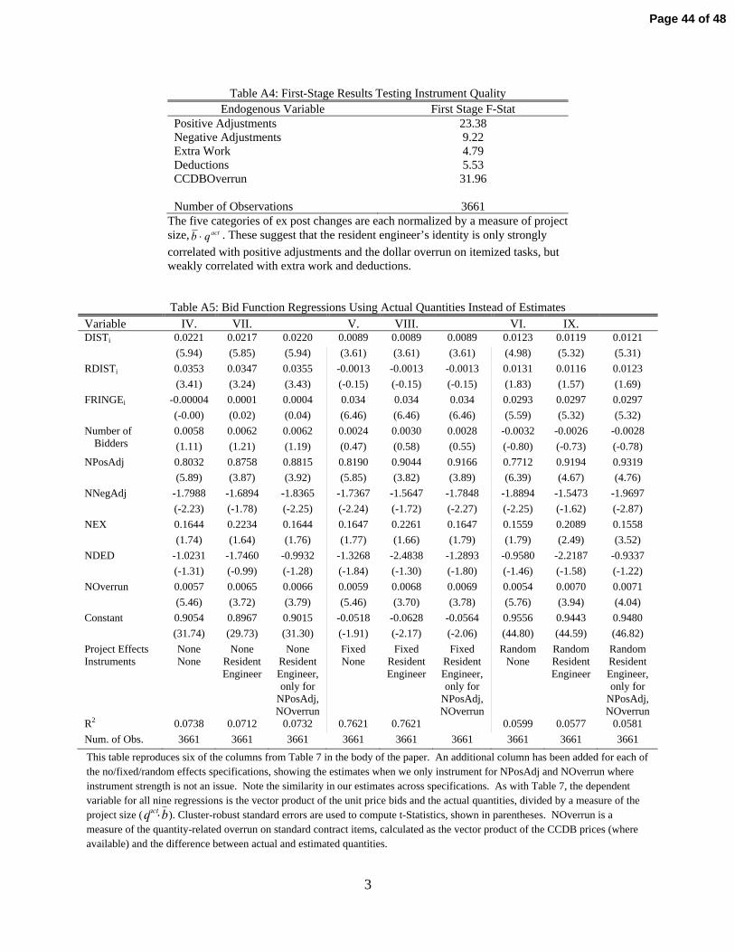
3
Table A4: First-Stage Results Testing Instrument Quality Endogenous Variable First Stage F-Stat
Positive Adjustments 23.38 Negative Adjustments 9.22 Extra Work 4.79 Deductions 5.53 CCDBOverrun 31.96 Number of Observations
3661
The five categories of ex post changes are each normalized by a measure of project size, actqb . These suggest that the resident engineer’s identity is only strongly
correlated with positive adjustments and the dollar overrun on itemized tasks, but weakly correlated with extra work and deductions.
Table A5: Bid Function Regressions Using Actual Quantities Instead of Estimates Variable IV. VII. V. VIII. VI. IX. DISTi 0.0221 0.0217 0.0220 0.0089 0.0089 0.0089 0.0123 0.0119 0.0121
(5.94) (5.85) (5.94) (3.61) (3.61) (3.61) (4.98) (5.32) (5.31)
RDISTi 0.0353 0.0347 0.0355 -0.0013 -0.0013 -0.0013 0.0131 0.0116 0.0123
(3.41) (3.24) (3.43) (-0.15) (-0.15) (-0.15) (1.83) (1.57) (1.69)
FRINGEi -0.00004 0.0001 0.0004 0.034 0.034 0.034 0.0293 0.0297 0.0297
(-0.00) (0.02) (0.04) (6.46) (6.46) (6.46) (5.59) (5.32) (5.32)
Number of Bidders
0.0058 0.0062 0.0062 0.0024 0.0030 0.0028 -0.0032 -0.0026 -0.0028
(1.11) (1.21) (1.19) (0.47) (0.58) (0.55) (-0.80) (-0.73) (-0.78)
NPosAdj 0.8032 0.8758 0.8815 0.8190 0.9044 0.9166 0.7712 0.9194 0.9319
(5.89) (3.87) (3.92) (5.85) (3.82) (3.89) (6.39) (4.67) (4.76)
NNegAdj -1.7988 -1.6894 -1.8365 -1.7367 -1.5647 -1.7848 -1.8894 -1.5473 -1.9697
(-2.23) (-1.78) (-2.25) (-2.24) (-1.72) (-2.27) (-2.25) (-1.62) (-2.87)
NEX 0.1644 0.2234 0.1644 0.1647 0.2261 0.1647 0.1559 0.2089 0.1558
(1.74) (1.64) (1.76) (1.77) (1.66) (1.79) (1.79) (2.49) (3.52)
NDED -1.0231 -1.7460 -0.9932 -1.3268 -2.4838 -1.2893 -0.9580 -2.2187 -0.9337
(-1.31) (-0.99) (-1.28) (-1.84) (-1.30) (-1.80) (-1.46) (-1.58) (-1.22)
NOverrun 0.0057 0.0065 0.0066 0.0059 0.0068 0.0069 0.0054 0.0070 0.0071
(5.46) (3.72) (3.79) (5.46) (3.70) (3.78) (5.76) (3.94) (4.04)
Constant 0.9054 0.8967 0.9015 -0.0518 -0.0628 -0.0564 0.9556 0.9443 0.9480
(31.74) (29.73) (31.30) (-1.91) (-2.17) (-2.06) (44.80) (44.59) (46.82)
Project Effects None None None Fixed Fixed Fixed Random Random Random Instruments None Resident
Engineer Resident Engineer, only for
NPosAdj, NOverrun
None Resident Engineer
Resident Engineer, only for
NPosAdj, NOverrun
None Resident Engineer
Resident Engineer, only for
NPosAdj, NOverrun
R2 0.0738 0.0712 0.0732 0.7621 0.7621 0.0599 0.0577 0.0581
Num. of Obs. 3661 3661 3661 3661 3661 3661 3661 3661 3661
This table reproduces six of the columns from Table 7 in the body of the paper. An additional column has been added for each of the no/fixed/random effects specifications, showing the estimates when we only instrument for NPosAdj and NOverrun where instrument strength is not an issue. Note the similarity in our estimates across specifications. As with Table 7, the dependent variable for all nine regressions is the vector product of the unit price bids and the actual quantities, divided by a measure of the project size ( bqact ). Cluster-robust standard errors are used to compute t-Statistics, shown in parentheses. NOverrun is a measure of the quantity-related overrun on standard contract items, calculated as the vector product of the CCDB prices (where available) and the difference between actual and estimated quantities.
Page 44 of 48
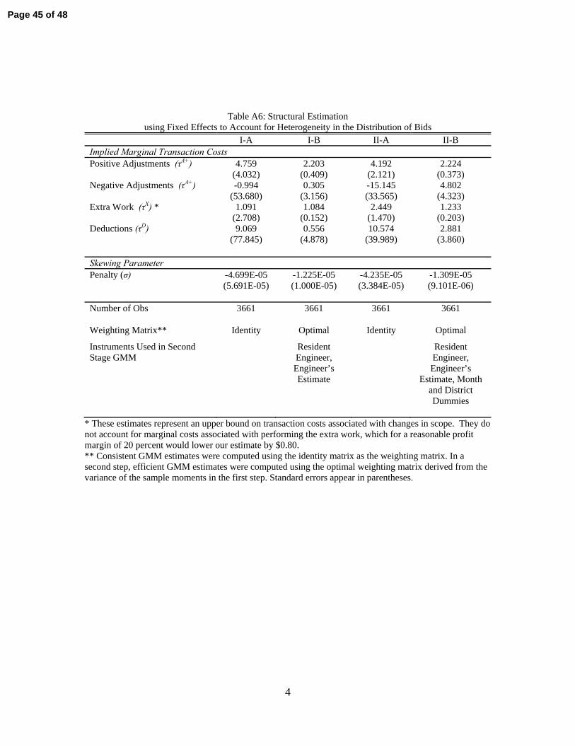
4
Table A6: Structural Estimation using Fixed Effects to Account for Heterogeneity in the Distribution of Bids
I-A I-B II-A II-B Implied Marginal Transaction Costs Positive Adjustments (τA+) 4.759 2.203 4.192 2.224
(4.032) (0.409) (2.121) (0.373) Negative Adjustments (τA+) -0.994 0.305 -15.145 4.802
(53.680) (3.156) (33.565) (4.323) Extra Work (τX) * 1.091 1.084 2.449 1.233
(2.708) (0.152) (1.470) (0.203) Deductions (τD) 9.069 0.556 10.574 2.881
(77.845) (4.878) (39.989) (3.860) Skewing Parameter Penalty (σ) -4.699E-05 -1.225E-05 -4.235E-05 -1.309E-05 (5.691E-05) (1.000E-05) (3.384E-05) (9.101E-06)
Number of Obs 3661 3661 3661 3661
Weighting Matrix** Identity Optimal Identity Optimal
Instruments Used in Second Stage GMM
Resident Engineer, Engineer’s Estimate
Resident Engineer, Engineer’s
Estimate, Month and District Dummies
* These estimates represent an upper bound on transaction costs associated with changes in scope. They do not account for marginal costs associated with performing the extra work, which for a reasonable profit margin of 20 percent would lower our estimate by $0.80. ** Consistent GMM estimates were computed using the identity matrix as the weighting matrix. In a second step, efficient GMM estimates were computed using the optimal weighting matrix derived from the variance of the sample moments in the first step. Standard errors appear in parentheses.
Page 45 of 48
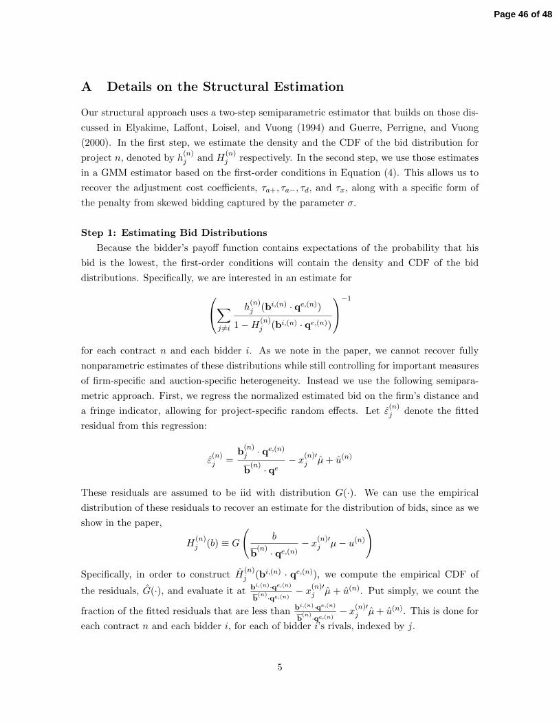
A Details on the Structural Estimation
Our structural approach uses a two-step semiparametric estimator that builds on those dis-
cussed in Elyakime, Laffont, Loisel, and Vuong (1994) and Guerre, Perrigne, and Vuong
(2000). In the first step, we estimate the density and the CDF of the bid distribution for
project n, denoted by h(n)j and H
(n)j respectively. In the second step, we use those estimates
in a GMM estimator based on the first-order conditions in Equation (4). This allows us to
recover the adjustment cost coefficients, τa+, τa−, τd, and τx, along with a specific form of
the penalty from skewed bidding captured by the parameter σ.
Step 1: Estimating Bid Distributions
Because the bidder’s payoff function contains expectations of the probability that his
bid is the lowest, the first-order conditions will contain the density and CDF of the bid
distributions. Specifically, we are interested in an estimate for∑j 6=i
h(n)j (bi,(n) · qe,(n))
1 −H(n)j (bi,(n) · qe,(n))
−1
for each contract n and each bidder i. As we note in the paper, we cannot recover fully
nonparametric estimates of these distributions while still controlling for important measures
of firm-specific and auction-specific heterogeneity. Instead we use the following semipara-
metric approach. First, we regress the normalized estimated bid on the firm’s distance and
a fringe indicator, allowing for project-specific random effects. Let ε(n)j denote the fitted
residual from this regression:
ε(n)j =
b(n)j · qe,(n)
b(n) · qe
− x(n)′j µ+ u(n)
These residuals are assumed to be iid with distribution G(·). We can use the empirical
distribution of these residuals to recover an estimate for the distribution of bids, since as we
show in the paper,
H(n)j (b) ≡ G
(b
b(n) · qe,(n)
− x(n)′j µ− u(n)
)
Specifically, in order to construct H(n)j (bi,(n) · qe,(n)), we compute the empirical CDF of
the residuals, G(·), and evaluate it at bi,(n)·qe,(n)
b(n)·qe,(n)
− x(n)′j µ + u(n). Put simply, we count the
fraction of the fitted residuals that are less than bi,(n)·qe,(n)
b(n)·qe,(n)
− x(n)′j µ+ u(n). This is done for
each contract n and each bidder i, for each of bidder i’s rivals, indexed by j.
5
Page 46 of 48
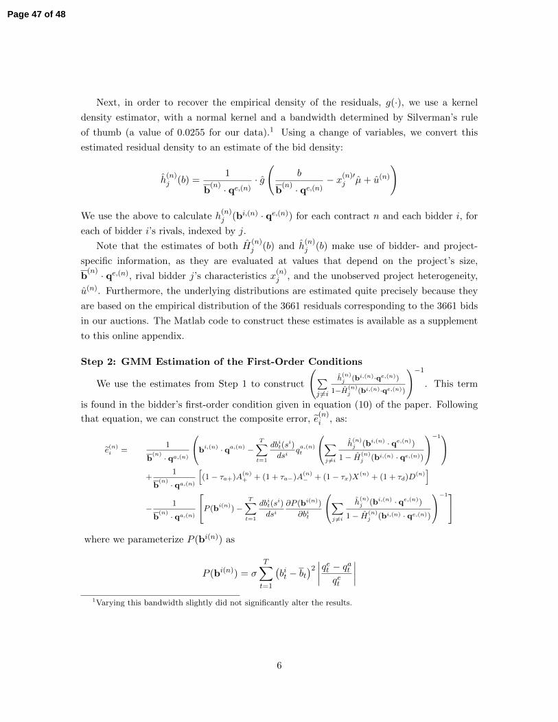
Next, in order to recover the empirical density of the residuals, g(·), we use a kernel
density estimator, with a normal kernel and a bandwidth determined by Silverman’s rule
of thumb (a value of 0.0255 for our data).1 Using a change of variables, we convert this
estimated residual density to an estimate of the bid density:
h(n)j (b) =
1
b(n) · qe,(n)
· g
(b
b(n) · qe,(n)
− x(n)′j µ+ u(n)
)
We use the above to calculate h(n)j (bi,(n) · qe,(n)) for each contract n and each bidder i, for
each of bidder i’s rivals, indexed by j.
Note that the estimates of both H(n)j (b) and h
(n)j (b) make use of bidder- and project-
specific information, as they are evaluated at values that depend on the project’s size,
b(n) · qe,(n), rival bidder j’s characteristics x
(n)j , and the unobserved project heterogeneity,
u(n). Furthermore, the underlying distributions are estimated quite precisely because they
are based on the empirical distribution of the 3661 residuals corresponding to the 3661 bids
in our auctions. The Matlab code to construct these estimates is available as a supplement
to this online appendix.
Step 2: GMM Estimation of the First-Order Conditions
We use the estimates from Step 1 to construct
(∑j 6=i
h(n)j (bi,(n)·qe,(n))
1−H(n)j (bi,(n)·qe,(n))
)−1. This term
is found in the bidder’s first-order condition given in equation (10) of the paper. Following
that equation, we can construct the composite error, e(n)i , as:
e(n)i =
1
b(n) · qa,(n)
bi,(n) · qa,(n) −T∑
t=1
dbit(si)
dsiqa,(n)t
∑j 6=i
h(n)j (bi,(n) · qe,(n))
1 − H(n)j (bi,(n) · qe,(n))
−1+
1
b(n) · qa,(n)
[(1 − τa+)A
(n)+ + (1 + τa−)A
(n)− + (1 − τx)X(n) + (1 + τd)D(n)
]
− 1
b(n) · qa,(n)
P (bi(n)) −T∑
t=1
dbit(si)
dsi∂P (bi(n))
∂bit
∑j 6=i
h(n)j (bi,(n) · qe,(n))
1 − H(n)j (bi,(n) · qe,(n))
−1where we parameterize P (bi(n)) as
P (bi(n)) = σT∑t=1
(bit − bt
)2 ∣∣∣∣qet − qatqet
∣∣∣∣1Varying this bandwidth slightly did not significantly alter the results.
6
Page 47 of 48
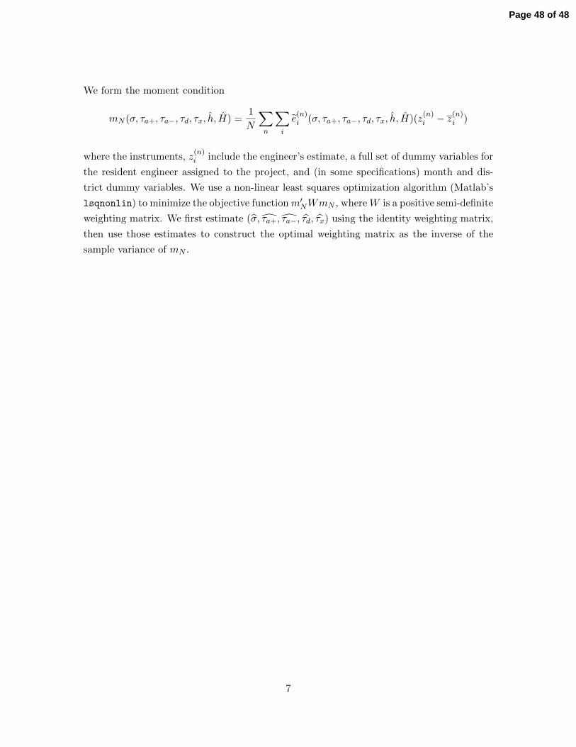
We form the moment condition
mN (σ, τa+, τa−, τd, τx, h, H) =1
N
∑n
∑i
e(n)i (σ, τa+, τa−, τd, τx, h, H)(z
(n)i − z
(n)i )
where the instruments, z(n)i include the engineer’s estimate, a full set of dummy variables for
the resident engineer assigned to the project, and (in some specifications) month and dis-
trict dummy variables. We use a non-linear least squares optimization algorithm (Matlab’s
lsqnonlin) to minimize the objective functionm′NWmN , whereW is a positive semi-definite
weighting matrix. We first estimate (σ, τa+, τa−, τd, τx) using the identity weighting matrix,
then use those estimates to construct the optimal weighting matrix as the inverse of the
sample variance of mN .
7
Page 48 of 48