asset class and portfolio risk and return

ASSET CLASSAND PORTFOLIO RISK

AND RETURNMethodology Overview

TABLE OF CONTENTSOVERVIEW .................................................................... 1

What is This Document? ..................................................1ASSET CLASS RISK ..................................................... 2

Risk Model Overview ........................................................2Factor Model Approach ................................................2Types of Factor Models ................................................3

Model Creation ..................................................................3Factor Selection ..............................................................3Covariance Matrix Construction ............................... 4EWMA Approach ..........................................................5MLE Approach ................................................................5Validating the Matrix ....................................................6Measuring Factor Exposures .......................................6Measuring Idiosyncratic Risk ......................................6Uncertainty in Asset Class Expectations .................7Confidence Intervals ......................................................7Mean Reversion in Asset Class Returns ...................7Statistical Evidence of Mean Reversion ....................8

Portfolio Analytics ........................................................... 16Portfolio Return and Risk ............................................ 16Efficient Frontier ........................................................... 17Simulated Efficient Frontier ....................................... 19Results ............................................................................20

REFERENCES ............................................................................................................ 22

REVISION DATE: 7/1/2015

ASSET CLASS RISK | 1

OVERVIEWWhat is This Document?

This is one in a series of plain-language white papers setting forth Research Affiliates’ building block approach to developing long-term capital market expectations by asset class. (For information about the objectives and

guiding principles of our asset allocation initiative, please refer to “Capital Market Expectations: Methodology Overview,” the first of these white papers.) In working out our risk and return forecasts and making them publicly available, we keep three criteria in mind: transparency, robustness, and timeliness. By describing the conceptual framework and calculations behind the projected asset class risks, returns, and correlations in these papers, we hope to achieve a meaningful level of transparency without excessive details. By constructing simple, economically sound models for major asset classes, we strive to achieve a fitting standard of robustness for forecasting to a 10-year horizon. By initially refreshing our expectations on a quarterly basis, we seek to provide information that is updated with useful frequency. We will continue to refine our methods, extend the scope of our capital market expectations, and improve this documentation over time.The remainder of this document addresses how we think about asset class risk, and provides transparency into the methods employed to develop these risk forecasts.

“We understand that some of our insights will never find their way into products, but we provide them in support of investors and the finance community.”

— ROB ARNOTTCHAIRMAN & CEO

2 | ASSET CLASS RISK

This document outlines the process of estimating risk for asset classes, quantifying uncertainty in capital market expectations over short time horizons, and combining asset class risk-and-return expectations into portfolios

that investors can use.

Asset Class RiskRisk Model Overview

A corollary to expected returns forecasting is forecasting asset class risk. This is most commonly done by measuring volatility and correlations,1, 2 either directly between the asset classes using historical time series

or indirectly through the use of factor models.

The asset class approach entails directly forecasting the volatility and correlations of the asset class pairs and results in a covariance matrix that grows as the number of asset classes in the investment universe grows.

The factor model approach provides a layer of abstraction by modeling characteristics common to asset classes rather than modeling the asset classes themselves. Asset class risk is measured by mapping the asset classes to the factors via a set of exposures. If the factor set is comprehensive, the factor model framework also allows new assets to be easily added to the investment opportunity set by simply measuring exposures to the set of factors.

In this document, we describe the factor model approach.

FACTOR MODEL APPROACH

Factor models grew out of the research of Stephen Ross, who broached the topic in his description of arbitrage pricing theory (APT) in his article “The Arbitrage Theory of Capital Asset Pricing” published in 1976. He left the details of specific factor definition to other research, however.

The basic equation for calculating an asset-class covariance matrix (∑) using a factor model is

(1)

In the equation, beta (β) represents the exposure of each investment to each factor; omega (Ω) represents the factor covariance matrix, which contains the variance of each factor and the covariance of each factor pair; and D represents the idiosyncratic risk component of each asset. This framework can be used to identify the risk of each asset and is used in portfolio construction, as described later.

The resultant asset-class covariance matrix contains, on the diagonal of the matrix, the variance of each asset, and in the off-diagonal terms, the asset’s covariance with the other assets in the matrix.

1As used in this document, correlation refers to Pearson correlation. 2We focus on volatility and correlation as the measures of risk, but investors should also consider higher moments, such as skewness, as alternative measures of risk

D∑ = β Ω β +T


TYPES OF FACTOR MODELS

A large literature on factor models exists. The three types of factor models most commonly used are statistical, explicit, and implicit (Baturin, Cahan, and He, 2014). All three have the same functional form as described in the previous section, but are very different in nature.

A statistical model utilizes principal component analysis to identify the sources of risk in a set of asset classes as a set of purely statistical factors. The benefit of this type of model is that it requires, from a data perspective, nothing more than a time series of asset class returns. The challenge is that, because the factors are statistical in nature, they often lack economic intuitiveness. Therefore, although these models provide a robust mechanism for capturing risk, it may come at the expense of the intuitive understanding necessary to make investment decisions.

An explicit factor model is likewise convenient because it also only requires a time series of asset class returns. These models construct factors based on time series data, often by constructing long/short portfolios of two or more assets. A covariance matrix is then assembled based on the time series volatility of each factor and the correlation between each pair of factors. Exposures of each investment to the factors are then determined.

The third type of factor model, an implicit factor model, uses a cross-section of fundamental information. Unlike the explicit model, which directly measures factor returns and then determines, through regression or other means, exposures to those factors, implicit models use fundamental information to directly measure exposures. For example, price-to-book ratio could be used to measure the exposure of an asset to a value factor. Once the exposures of the asset universe are calculated, cross-sectional regression is used to generate the factor returns. The volatility and covariance of those factor returns over time is then used to generate a covariance matrix. Although implicit factor models have proven to be very useful, they can be very costly from a data and analytics perspective. Using an implicit factor model requires access not only to asset returns, but to fundamental information about each asset.

The remainder of this document focuses on constructing and using an explicit factor model.3

Model Creation

We now turn our attention to the process of factor selection and the mechanical construction of the factor and asset-class covariance matrices.

FACTOR SELECTION

In this model, factor selection involves identifying the set of characteristics that ultimately drive risk and return. Each of the factors is created as a zero investment (long/short) portfolio of asset classes with the goal of creating factors that are able to capture various sources of return premia. Modeling sources of return across a broad set of asset classes requires inclusion of a large list of factors, such as those specified in Table 1.

3Some readers may wonder why we use a factor model at all. If the set of asset classes in question is diverse enough, the set of factors needed to model those assets will map one- to- one to the assets themselves. In this case, generating a factor model is nothing more than reorganizing the assets in a different form. We acknowledge this to be true, but creating a factor model allows us to easily replicate an ever expanding list of assets as well as to explain the process of constructing factor models to readers who are unfamiliar with the methodology.


Risk Factor Long Index Short Index

Real Cash U.S. T-bills U.S. CPI

Market S&P 500 U.S. T-bills

Value Russell 1000 Value Russell 1000 Growth

Size Russell 2000 S&P 500

Country MSCI Country S&P 500

U.S. Short Duration Barclays US Treasury 1-3 Year U.S. T-bills

U.S. Mid Duration Barclays US Treasury 3-7 Year Barclays US Treasury 1-3 Year

U.S. Long Duration Barclays US Treasury 7-10 Year Barclays US Treasury 3-7 Year

U.S. Credit Spread Barclays Intermediate Credit Barclays US Treasury 3-7 Year

U.S. HY Credit Spread Barclays Corporate High Yield Barclays Intermediate Credit

EM Hard Currency Spread JPM EMBI+ Barclays US Treasury 3-7 Year

EM Local Currency Spread JPM GBI-EM Barclays US Treasury 3-7 Year

REITS FTSE NAREIT U.S. T-bills

Commodities Bloomberg Commodity U.S. T-bills

Creating factors as long/short portfolios is beneficial because it isolates return premia and allows us to reduce collinearity between factors, which could otherwise cause spurious correlations to appear when measuring the exposure of securities to the factors.4

COVARIANCE MATRIX CONSTRUCTIONThe covariance matrix is generated by calculating the covariance between each pair of factors. Two important considerations in constructing the covariance matrix are the amount of historical data to include and the method of weighting the data.

The simplest solution is to include all available data. In a perfect world, all factors would have an identical length and span of data history, and this would be a fine approach; in the real world, however, factors have very different time histories. For example, a U.S. market equity factor that uses the S&P 500 Index may have data for 100 years or more, whereas an emerging markets (EM) equity factor may have only 30 years of reliable history. When factors have different lengths of data history, using a full time series for each factor with all data weighted equally results in an unpredictable covariance matrix.

TABLE 1Selected Factors Used to Model Asset Class Risk

Source: Research Affiliates, LLC

4In creating the long/short portfolios, it is vital to make sure risk premia are isolated and are not corrupted by extraneous risks. For example, in creating a credit-spread factor, care should be taken to match the duration of the indices used in isolating a particular credit spread.


In an effort to be consistent, it is possible to restrict the historical data used to construct the covariance matrix to a time interval shared by the factors. The obvious drawback of this approach is that a considerable amount of data could be ignored, such as in the previous example of 100 or more years of U.S. equity returns restricted to 30 years of EM equity returns. Restricting data to a common time window would cause decades of U.S. data to be discarded and along with it the information contained in that data. This is not an ideal approach, which leads us to consider another possible weighting scheme.

EWMA APPROACHInstead of equally weighting data samples, as is done in a simple calculation of covariance, another approach is to create an exponentially weighted moving average (EWMA) as described by Jorion (2006). The EWMA weights the data so as to de-emphasize older time samples.

The EWMA methodology is based on a decay factor, lambda (λ), which dictates the rate at which older data is de-emphasized. The decay factor defines the half-life, the point at which the data are weighted at 50% of original value. The half-life we use is 120 months, which means that 10-year-old data are weighted one-half as much as current data, data that are 20 years old are weighted one-quarter as much, and so on. The EWMA equation, which follows, shows how recursively multiplying older returns by λ reduces their significance:

(2)

By de-emphasizing very old data, the EWMA approach addresses the issue of disparity in time histories across asset classes. Instead of, or even in addition to, weighting samples differently over time, it is also possible to infer historical data in order to extend shorter time series via the maximum likelihood estimator approach, which is discussed in the next section.

MLE APPROACHThe maximum likelihood estimator (MLE) approach, as described by Stambaugh (1997), uses ordinary least squares (OLS) regression to identify the relationship between two time series over the common period in which they both have data. The resultant regression equations are then used to estimate additional history for the shorter time series going back in time. Because this approach simulates data, care should be taken in examining the results of the regressions and the amount of history that is being estimated. Even with these precautions, however, the MLE approach is a strong method of addressing disparity in the histories of data series.

Once the issue of time-series length has been addressed, the covariance matrix can be easily generated using textbook equations for calculating variance and covariance.

( )2 2 21 11 − −σ = − λ × + λ × σt t tr

11where 2

−λ =

half life


VALIDATING THE MATRIXIt is important to test the covariance matrix that has been generated in order to verify that it is positive semi-definite. Because the diagonal of the covariance matrix represents variance values, which are the squares of volatilities, negative values on the diagonal would be nonsensical.

Testing that the matrix is positive semi-definite is done by ensuring that all the eigenvalues, or equivalently, all of the pivots, of the matrix are greater than or equal to zero.

MEASURING FACTOR EXPOSURESOnce the covariance matrix is constructed, the exposure of each asset in the investment universe must be measured versus each factor. This can be done by running an OLS regression of the returns of the asset class, the dependent variable, against the returns of each of the factors, the independent variables, as follows, where the regression coefficients are the exposures of the asset class to each factor:

(3)

Using an OLS regression to identify exposures does have a downside. First, because it can be difficult to construct a set of factors that are completely uncorrelated, the collinearity between factors can lead to noisy exposures that do not measure the true magnitude of the economic drivers of the risk and return of the asset class. Although it is easy to say that factors need to be uncorrelated, in practice this can be hard to achieve.

Second, although OLS will give the best fit of the historical data, the regression results may not be the best predictor of future outcomes. For example, consider an aggregate index, such as the Barclays U.S. Aggregate Bond Index. An OLS regression of this index on a set of bond factors will result in an exposure to sovereign, credit, and structured product factors. These exposures will do a good job of fitting the historical weights of the index to the factors, but they will not be effective in capturing a structural change in the composition of the index. Thus, if the index provider changes the structure of the index to better capture the distribution characteristics of the outstanding debt in an economy, such information would be missed in the OLS results and be unavailable to inform ex ante return forecasts.5

Before addressing these two issues—noisy exposures and unreliable forecasts—it is important to have an opinion regarding the exposure of each asset class to each factor. Establishing an opinion before running the OLS regression provides two sources of data for determining the best exposure set to use in the factor model. In some cases, a prior belief will be validated by the OLS results, and often the OLS results add useful information to the decision-making process.

MEASURING IDIOSYNCRATIC RISKThe idiosyncratic risk describes the volatility of the residual (ε) of the regression equation, or the difference between the actual and estimated returns (“hat” variables):

(4)

5The Barclays U.S. Aggregate is used as a hypothetical example and is not meant to imply that a structural change has recently occurred or is expected to occur in the index in the near future.

,1==α + ∑ β × + εN

t i i t tir F

( )2 2σ = σ −residual t tr r

,1

ˆˆˆ=

=α + β ×∑N

t i i ti

where r F


The D term in Equation (1) is an “n × n” matrix, where “n” represents the number of asset classes. The diagonal of the matrix represents the variance of the residual of each asset, with the off-diagonal terms being equal to zero.

UNCERTAINTY IN ASSET CLASS EXPECTATIONSWith the information provided in this document, along with the information provided in the other documents in the Research Affiliates online library, it is possible to generate point forecasts for expected risk and return across asset classes. We now turn our attention to measuring the uncertainty that accompanies the use of long-term forecasts over shorter time horizons.

The foundation for the expected-return point forecast is the fact that if the time horizon is long enough, realized returns will average out to the expectation, and as the time horizon (in this case measured in years) shortens, the variability of returns around the point forecast increases.

To put this variability into context, take, for example, an equity index with a 10-year average expected return. Now consider that someone with perfect foresight gives you a bag of ping pong balls, one for each future year, and on each ball is written the return that will be earned in that year. If you pull 10 balls from the bag and average them, it is very likely that the result will differ from the 10-year average expected return. If, however, the experiment is repeated a large number of times and the results are plotted on a histogram, a distribution will emerge whose average will be equal to the expected return.6

CONFIDENCE INTERVALSA simple estimation of the confidence interval is calculated as the expected-return point forecast, plus or minus the size of the interval, multiplied by the standard error of the estimate (standard deviation divided by the square root of the number of samples, T, in the investment horizon):7

(5)

From this equation, it is easy to see that as the number of samples, T, goes to infinity, the interval, as expected, collapses to the point forecast. Certain assumptions underlying this equation, which affect the results, are not applicable to asset class returns.

In particular, calculating the standard error in this way assumes that each annual return is both independent and identically distributed (i.i.d.) such that the covariance between annual returns is zero (Diebold et al., 1998).

MEAN REVERSION IN ASSET CLASS RETURNSIn real life, however, asset class returns experience both momentum and mean reversion (MMR), and the standard error should be enhanced to take this into account.

6In this situation, the expected return and volatility are assumed to be unbiased estimators (i.e., the true statistics) for the future return of each asset class (i.e., any model misspecification risk is assumed to be zero).7We have parameterized the number of samples (years in the investment horizon or single-experiment ping pong balls pulled from the bag in the example in the previous section) as T = 10. Alternatively, the standard error could be calculated from an OLS regression of the expected and realized returns. Here we are using the z-distribution, but because of the size of T, others may decide to use the Student’s t-distribution.

[ ] [ ]Confidence Interval σ= ± × = ± ×Annualized Annual AnnualE r Z SE E r Z

T


STATISTICAL EVIDENCE OF MEAN REVERSIONAs Alexander (2008) discusses, MMR can be measured by the autocorrelation of returns within each asset class using an AR(1) model; autocorrelation values greater than zero indicate momentum in returns, whereas values less than zero signify mean reversion.

In the following equation, T is the number of lagged periods, and δ is the AR(1) autocorrelation coefficient:

(6)

The MMR value can then be integrated into the confidence interval equation,

(7)

Figure 1 shows changes in per annum volatility for various autocorrelation values, based on an i.i.d. volatility of 15%. On the left side of the figure, autocorrelation values are below zero, denoting mean reversion and a reduction in volatility, whereas on the right side of the figure, the autocorrelation values are above zero, denoting momentum and a rise in volatility.

[ ] MMR Confidence Interval Annualized AnnualE r Z MMRT

σ= ± × ×

( )( ) ( ) ( )

12

12

1MMR 2 1 1 11

− δ = + − − δ − δ − δ × + δ

T T TT


FIGURE 1Per Annum Volatility for Autocorrelation Values of an Index with 15% Volatility

0.0%

6.5%9.2%

11.9%

15.0%

18.8%

24.2%

32.6%

46.7%

0%

10%

20%

30%

40%

50%

-1 -0.5 0 0.5 1

VO

LATI

LITY

(P.A

.)

AUTOCORRELATION


Figure 2 shows annual, non-overlapping, autocorrelation results for the S&P 500. Unfortunately, the autocorrelation coefficients at a 10-year horizon are not statistically significant.8 The same results are seen in the bond, currency, and commodity asset classes.

8All references in this paper to statistical significance are at the 95% level.


In order to further test the statistical significance of mean reversion, we calculate variance ratios (Lo and MacKinlay, 1988) based on monthly periods out to 120 months.10, 11 The tests show some amount of mean reversion at longer time periods, but the findings are not significant. Here we only include the variance ratio chart for equities, but other asset classes show similar results.

We analyze the variance ratio results because they, as well as other tests, are often included in articles on asset-class mean reversion. The lack of statistical significance of the tests is not unexpected. In fact, it is known that most statistical tests—including unit root, regression based, and maximum likelihood—are not powerful enough tools to identify mean reversion. Unfortunately, this is an example of when more data cannot improve the outcome.

FIGURE 2Autocorrelation of Annual Returns of S&P 500, 1926–2014 (p-value of Box–Pierce9 = 0.86)

-0.4

-0.2

0

0.2

0.4

0.6

0.8

1

0 2 4 6 8 10 12 14 16 18

AU

TOCO

RREL

ATI

ON

LAG

Source: Research Affiliates, LLC, based on data from Bloomberg.

9The Box–Pierce test measures the statistical significance of the autocorrelation residuals.10“Variance ratios are among the most powerful tests for detecting mean reversion,” according to Poterba and Summers (1988). The variance ratio test is based on the idea that if a series is stationary, the variance of the series should not change over time; a series with a unit root, however, should have a changing variance. Comparing the variance of a time series of returns to the variance of lagged returns, VR(q) = σ2 (q) /σ2 (1), will result in a value of one (random walk), values greater than one (momentum), or values less than one (mean reversion).11We use monthly periods to show additional granularity in the figures, but the results using annual periods are consistent with the monthly results.


FIGURE 2Autocorrelation of Annual Returns of S&P 500, 1926–2014 (p-value of Box–Pierce9 = 0.86)

Given the data shown in Figure 3 and the lack of statistical significance in mean reversion, it would be easy to revert to the simple confidence interval as the best estimate of asset class returns, but doing so would ignore the fact that empirical mean reversion is observed in asset class returns. Figures 4–6 show volatility of annualized returns for equity (S&P 500), bond (Barclays Global Aggregate), and commodity (S&P GSCI) indices for investment time horizons of 1–10 years12 and compares the values to an estimated volatility computed by dividing one-year volatility by the square root of T.

FIGURE 3S&P 500 Variance Ratio (1926–2015), Monthly

0

0.5

1

1.5

2

0 20 40 60 80 100 120

VA

RIA

NCE

RA

TIO

HOLDING PERIOD (MONTHS)

Source: Research Affiliates, LLC, based on data from Bloomberg.

12The x axis represents the time horizon. Therefore, plot points with an x coordinate of five show annualized five-year returns. These charts are based on year-end data.


FIGURE 4S&P 500 Volatility of Annualized Returns at 1–10 Year Horizons, 1926–2015

0%

5%

10%

15%

20%

25%

1 2 3 4 5 6 7 8 9 10

VO

LATI

LITY

YEARS

ACTUAL VOL SQRT(T) ESTIMATED VOL



FIGURE 5Barclays Global Aggregate Volatility of Annualized Returns at 1–10 Year Horizons, 1990–2015

0%

1%

2%

3%

4%

5%

6%

7%

1 2 3 4 5 6 7 8 9 10

VO

LATI

LITY

YEARS




Across asset classes, at longer time horizons, the historically realized volatility of returns is lower than an estimate of volatility based on scaling the one-year volatility by 1/√T, which implies mean reversion does exist. Table 2 quantifies the difference at a 10-year investment horizon.

FIGURE 6S&P GSCI Commodity Index Volatility of Annualized Returns at 1–10 Year Time Horizons, 1970–2015

0%

5%

10%

15%

20%

25%

30%

1 2 3 4 5 6 7 8 9 10

VO

LATI

LITY

YEARS




Thus, if we ignore mean reversion, confidence intervals would be 15% larger for equities and commodities, and 85% larger for global bonds, than has been empirically observed. Figure 7 reports the results when the sample is extended to a much larger set of 55 indices across equities, bonds, and commodities.

TABLE 2Comparing the Square-Root-of-T Rule to Historical Returns

Asset Class Scaled 1-Year Volatility 10-Year Volatility Ratio

Equity 6.3% 5.5% 116%

Bond 2.0% 1.1% 185%

Commodity 5.9% 5.2% 115%


FIGURE 7Comparing the Square-Root-of-T Rule to Historical Returns for Indices across Asset Classes

y = 0.447xR² = 0.2316

0%

5%

10%

15%

20%

25%

30%

0% 5% 10% 15% 20% 25% 30%

10-Y

EAR

AN

NU

ALI

ZED

VO

L

1-YEAR ANNUAL VOL/SQRT(T)



If asset returns were i.i.d, in Figure 7 all the diamonds would line up on or near the 45-degree line. Instead, most of the diamonds—except those representing fixed income indices with very low volatility13—fall below the line. The R2, which equals 23%, is being pulled lower by the outlier index (MSCI Turkey) in the lower far-right area of the figure. Without the data point of MSCI Turkey, the R2 roughly doubles. Figure 7 illustrates that if we multiply the last term of Equation (6), 1/√T , by 1/2 , the result is a more appropriate measure of the confidence interval. We, therefore, use this 1/2 scalar in our confidence interval calculations, as follows:

Portfolio Analytics

Now, let’s turn our attention to creating portfolios from individual asset class risk-and-return expectations.

PORTFOLIO RETURN AND RISKIn discussing future returns, the two metrics most often referenced are the geometric expected mean (average growth of compounded wealth) and the arithmetic expected mean (probability weighted average of all possible future states of return). Each is the forward-looking corollary of its respective historical counterpart: the geometric mean and the arithmetic mean. Ibbotson and Chen (2003) observe that the arithmetic average is the measure of returns most often used in portfolio optimization. Kaplan (2012) adds additional context to the interplay between arithmetic and geometric expectations when he observes that in the Markowitz investment model, the relevant measure of reward is the expected (arithmetic) return. He notes that the case is different for long-term investors, who are more concerned with the long-term rate of portfolio growth, or the geometric mean.

Up to now, we have described a methodology for calculating the geometric expected return. The reason the results thus far are geometric in nature goes back to the derivation of the dividend discount model, which is based on a geometric series.

The nice thing about the geometric expected mean is that it provides an apples-to-apples comparison with the commonly used geometric mean of historical returns, also known as the compound annual growth rate of an asset. The downside of the geometric expected mean is that these returns cannot directly be used to create portfolios. As described by McCulloch (2003), the geometric return of a portfolio is not equal to the weighted average of the geometric returns of the portfolio’s constituents, as might be expected.

13During the majority of the sample period, interest rates declined in a near-linear trend. This downward trajectory in rates likely impacted the risk attributes of the fixed income indices. Greater volatility in interest rates over the last 40 years would likely have produced different results.

[ ] [ ]Confidence Interval2

σ= ± × = ± ×Annualized Annual AnnualE r Z SE E r Z

T


In order to find the geometric return of a portfolio, we must first convert each asset’s return to an arithmetic return, aggregate them based on a weighted average, and then convert the arithmetic portfolio return back to a geometric return. The following equation is an approximation, under the commonly held assumption of log normally distributed returns, which is used to convert back and forth between geometric and arithmetic returns:14

Given that the arithmetic mean is almost always larger than the geometric mean, it is no surprise that converting a geometric return to arithmetic involves adding an additional term. In this case that term, σ2/2, is one-half the variance of the asset class. The arithmetic return of each asset class is then aggregated into a single portfolio. This is done by multiplying the arithmetic return by the weight of each asset in the portfolio,

The asset-class covariance matrix can then be used to calculate the risk of the portfolio by multiplying the matrix by the weights of the individual assets in the portfolio, as follows:

Finally the geometric return of the portfolio can be determined by converting the arithmetic return using the calculated portfolio variance. From these portfolio point estimates, confidence intervals should also be calculated to account for the variability of expectations over shorter time horizons.

EFFICIENT FRONTIERThe efficient frontier is the only set of portfolios that a rational investor would choose, because, by definition, all other portfolios could be improved by either increasing return or decreasing risk. All that is required to create an efficient frontier is the set of expected risk-and-return forecasts for the asset class as well as a set of constraints, whose purpose is to prevent undesired outcomes, such as an overconcentration in a particular security or sector.

14A downside of using this approximation is that it assumes returns are independent over time, but that is not the case as previously discussed in the subsection on confidence intervals; that said, the formula is included here as a simple heuristic. McCulloch (2003) expounds on a more detailed relationship, as does Kaplan (2012), who shows that as the investment horizon grows longer.

, , 1

N

p arithmetic i i arithmetici

r w r=

= ×∑

[ ]2

2σ = + arithmetic geometricE r E r

2 ∑σ = Tp w w

[ ]( )[ ]( )

2

2 2

11

1

+ = −

+ + σ

arithmetic geometric

arithmetic

E rE r

E r


Two equally important questions govern the creation of portfolios based on expected risk-and-return metrics:

1. What is the maximum return for a given level of risk?

2. What is the minimum amount of risk that must be taken to ensure a specific level of return?

Answering these questions for all values of the risk or return dimension (for which a feasible solution exists) allows for the development of an efficient frontier of portfolios, as illustrated in Figure 8.

FIGURE 8Mean Variance Efficient Frontier

10%

11%

12%

13%

14%

15%

16%

15% 17% 19% 21% 23% 25% 27%

EXPE

CTED

RET

URN

S

VOLATILITY



Several concerns surround the creation of efficient portfolios. One concern is that by using expectation point forecasts alone, the optimizer15 used to generate the efficient frontier is forced to assume the inputs are exact and make the appropriate trade-offs. But as previously mentioned, the risk-and-return point forecasts are not exact; utilizing the confidence ranges around them would be beneficial in finding the efficient frontier.16

If we ignore the variability represented by the confidence ranges surrounding the point forecasts, we risk being overconfident in our resulting set of efficient portfolios. In addition, the optimizer could generate portfolios highly concentrated in a security, sector, or maturity. Minor, often insignificant, changes in the input parameters can also cause large swings in the constituents of the output portfolio. Investors who blindly follow the commensurate changes could incur large transaction costs, among other problems.

SIMULATED EFFICIENT FRONTIERWe adopt the process outlined by Jorion (1992) to include variability in the process of locating efficient portfolios. In this process, instead of calculating efficient portfolios using only expected risk-and-return point forecasts, we run a Monte Carlo simulation with 1,000 iterations to sample from the expected return distribution of each asset class and create optimal portfolios to meet the desired input condition. The optimal portfolios are calculated by averaging the asset class weights from each of the simulations.

Consider an example with only two runs—not a realistic simulation, but sufficient for illustrative purposes—and two asset classes: stocks and bonds, each with an expected return that is the mean of a distribution, quantified by confidence intervals. During each of the two Monte Carlo runs, an expected return for each asset will be selected from each respective asset class distribution for use in the optimization. Because the expected returns may change from run to run, the optimizer will create different portfolios each time. In this case, let’s say the first run generates a portfolio that is 60% stocks/40% bonds, and the second run generates a portfolio that is 57% stocks/43% bonds. Due to the uncertainty in the initial expectations, it is impossible to know if one portfolio is more efficient than the other. The solution is therefore to average the two portfolios together to get a final efficient portfolio composed of 58.5% stocks and 41.5% bonds.

We follow exactly the same process, but use a much larger number of runs. Figure 9 is an example histogram of a partial list of assets that make up a single efficient portfolio. The x-axis shows the weight of each asset in the portfolio, and the y-axis shows the number of simulations performed for each asset to determine that weight.

The same process is then run repeatedly for different levels of risk (or return) in order to generate a set of efficient portfolios. As the variability in the expected return inputs shrinks, these portfolios will approach the efficient frontier, based on the point forecasts alone, which can be thought of as the upper limit of the portfolios.

15The standard optimization equation we use is max w’ μ- 1/2 λw’ Σw, where w is the set of security weights, μ is the expected return, and Σ is the asset-class covariance matrix. The equation finds the maximum return for a given level of risk, which is scaled by a risk penalty defined by the risk aversion parameter lambda (λ). Investors with a higher risk aversion will have a higher risk penalty and thus will require a higher return per unit of risk taken. 16The same method described earlier is used to generate the confidence intervals, but in this case because we are dealing with portfolios, we multiply 1/(2√T) by the entire covariance matrix.


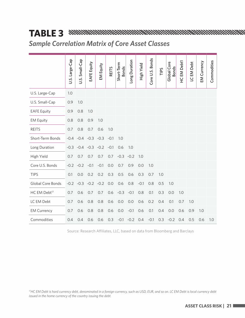
RESULTSPutting all of this together—implementing the EWMA process to generate a factor covariance matrix and then multiplying that matrix by a matrix of exposures of the core asset classes—results in an asset-class covariance matrix, or a corollary correlation matrix. Table 3 shows a sample of the correlation matrix derived from that covariance matrix. adopt the process outlined by Jorion (1992) to include variability in the process of locating efficient portfolios.

We can then generate portfolios, including a set of efficient portfolios by simulation, using the covariance matrix, the expected returns for each asset class, and a set of constraints. One constraint is the long-only weights have upper bounds, as described on the portfolio creation screen of the Asset Allocation site.

FIGURE 9Example of Portfolio Weights from Multiple Iterations

0

100

200

300

400

500

600

700

0 0.1 0.2 0.3 0.4

# O

F SA

MPL

ES

ASSET CLASS WEIGHT

SHORT-TERM BONDS LONG-TERM BONDS BANK LOANS EM EQUITY



U.S

. Lar

ge-C

ap

U.S

. Sm

all-C

ap

EAFE

Equ

ity

EM E

quity

REIT

S

Shor

t-Ter

m

Bond

s

Long

Dur

atio

n

Hig

h Yi

eld

Core

U.S

. Bon

ds

TIPS

Glo

bal C

ore

Bond

s

HC

EM D

ebt1

LC E

M D

ebt

EM C

urre

ncy

Com

mod

ities

U.S. Large-Cap 1.0

U.S. Small-Cap 0.9 1.0

EAFE Equity 0.9 0.8 1.0

EM Equity 0.8 0.8 0.9 1.0

REITS 0.7 0.8 0.7 0.6 1.0

Short-Term Bonds -0.4 -0.4 -0.3 -0.3 -0.1 1.0

Long Duration -0.3 -0.4 -0.3 -0.2 -0.1 0.6 1.0

High Yield 0.7 0.7 0.7 0.7 0.7 -0.3 -0.2 1.0

Core U.S. Bonds -0.2 -0.2 -0.1 -0.1 0.0 0.7 0.9 0.0 1.0

TIPS 0.1 0.0 0.2 0.2 0.3 0.5 0.6 0.3 0.7 1.0

Global Core Bonds -0.2 -0.3 -0.2 -0.2 0.0 0.6 0.8 -0.1 0.8 0.5 1.0

HC EM Debt17 0.7 0.6 0.7 0.7 0.6 -0.3 -0.1 0.8 0.1 0.3 0.0 1.0

LC EM Debt 0.7 0.6 0.8 0.8 0.6 0.0 0.0 0.6 0.2 0.4 0.1 0.7 1.0

EM Currency 0.7 0.6 0.8 0.8 0.6 0.0 -0.1 0.6 0.1 0.4 0.0 0.6 0.9 1.0

Commodities 0.4 0.4 0.6 0.6 0.3 -0.1 -0.2 0.4 -0.1 0.3 -0.2 0.4 0.5 0.6 1.0

Source: Research Affiliates, LLC, based on data from Bloomberg and Barclays

TABLE 3Sample Correlation Matrix of Core Asset Classes

17HC EM Debt is hard currency debt, denominated in a foreign currency, such as USD, EUR, and so on. LC EM Debt is local currency debt issued in the home currency of the country issuing the debt.


REFERENCES

Alexander, Carol. 2008. Practical Financial Econometrics. Hoboken, NJ: John Wiley & Sons, Inc.

Baturin, Nick, Ercument Cahan, and Kevin He. 2014. “US Equity Fundamental Factor Model.” Bloomberg.

Diebold, Francis X., Andrew Hickman, Atsushi Inoue, and Til Schuermann. 1998. “Converting 1-Day Volatility to h-Day Volatility: Scaling by Square Root-h Is Worse Than You Think.” Wharton Financial Institutions Center, Working Paper 97-34.

Ibbotson, Roger, and Peng Chen. 2003. “Long-Run Stock Returns: Participating in the Real Economy.” Financial Analysts Journal, vol. 59, no. 1 (January/February):88–98.

Jorion, Philippe. 1992. “Portfolio Optimization in Practice.” Financial Analysts Journal, vol. 48, no. 1 (January/February):68–74.

———. 2006. Value at Risk: The New Benchmark for Managing Financial Risk, 3rd ed. New York, NY: McGraw-Hill.

Kaplan, Paul D. 2011. Frontiers of Modern Asset Allocation. Hoboken, NJ: John Wiley & Sons, Inc.

Lo, Andrew W., and A. Craig MacKinlay. 1988. “Stock Market Prices Do Not Follow Random Walks: Evidence from a Simple Specification Test.” The Review of Financial Studies, vol. 1, no. 1 (Spring):41–66.

McCulloch, Brian W. 2003. “Geometric Return and Portfolio Analysis.” New Zealand Treasury, Working Paper No. 03/28.

Poterba, James M., and Lawrence H. Summers. 1988. “Mean Reversion in Stock Prices: Evidence and Implications.” Journal of Financial Economics, vol. 22, no. 1 (October):27–59.

Ross, Stephen A. 1976. “The Arbitrage Theory of Capital Asset Pricing.” Journal of Economic Theory, vol. 13, no. 3 (December):341–360.

Stambaugh, Robert F. 1997. “Analyzing Investments Whose Histories Differ in Length.” Journal of Financial Economics, vol. 45, no. 3 (September):285–331.


DISCLAIMER

The information contained herein regarding Asset Allocation and Expected Returns may represent real return forecasts for several asset classes and not for any Research Affiliates (“RA”) fund or strategy. These forecasts are forward-looking statements based upon the reasonable beliefs of RA and are not a guarantee of future performance. Forward-looking statements speak only as of the date they are made, and RA assumes no duty to and does not undertake to update forward-looking statements. Forward-looking statements are subject to numerous assumptions, risks, and uncertainties, which change over time. Actual results may differ materially from those anticipated in forward-looking statements.

All projections provided are estimates and are in U.S. dollar terms, unless otherwise specified. Given the complex risk-reward trade-offs involved, one should always rely on judgment as well as quantitative optimization approaches in setting strategic allocations to any or all of the above asset classes. Please note that all information shown is based on qualitative analysis. Exclusive reliance on the above is not advised. This information is not intended as a recommendation to invest in any particular asset class or strategy or as a promise of future performance. Note that these asset class and strategy assumptions are passive only–they do not consider the impact of active management. References to future returns are not promises or even estimates of actual returns a client portfolio may achieve. Assumptions, opinions and estimates are provided for illustrative purposes only. They should not be relied upon as recommendations to buy or sell any securities, commodities, derivatives or financial instruments of any kind. Forecasts of financial market trends that are based on current market conditions or historical data constitute a judgment and are subject to change without notice. We do not warrant its accuracy or completeness. This material has been prepared for information purposes only and is not intended to provide, and should not be relied on for, accounting, legal, tax, investment or tax advice. There is no assurance that any of the target prices mentioned will be attained. Any market prices are only indications of market values and are subject to change.

Hypothetical or simulated performance results have certain inherent limitations. Unlike an actual performance record, simulated results do not represent actual trading, but are based on the historical returns of the selected investments, indices or investment classes and various assumptions of past and future events. Simulated trading programs in general are also subject to the fact that they are designed with the benefit of hindsight. Also, since the trades have not actually been executed, the results may have under or over compensated for the impact of certain market factors. In addition, hypothetical trading does not involve financial risk. No hypothetical trading record can completely account for the impact of financial risk in actual trading. For example, the ability to withstand losses or to adhere to a particular trading program in spite of the trading losses are material factors which can adversely affect the actual trading results. There are numerous other factors related to the economy or markets in general or to the implementation of any specific trading program which cannot be fully accounted for in the preparation of hypothetical performance results, all of which can adversely affect trading results.

The asset classes are represented by broad-based indices which have been selected because they are well known and are easily recognizable by investors. Indices have limitations because indices have volatility and other material characteristics that may differ from an actual portfolio. For example, investments made for a portfolio may differ significantly in terms of security holdings, industry weightings and asset allocation from those of the index. Accordingly, investment results and volatility of a portfolio may differ from those of the index. Also, the indices noted in this presentation are unmanaged, are not available for direct investment, and are not subject to management fees, transaction costs or other types of expenses that a portfolio may incur. In addition, the performance of the indices reflects reinvestment of dividends and, where applicable, capital gain distributions. Therefore, investors should carefully consider these limitations and differences when evaluating the index performance.

No investment process is risk free and there is no guarantee of profitability; investors may lose all of their investments. No investment strategy or risk management technique can guarantee returns or eliminate risk in any market environment. Diversification does not guarantee a profit or protect against loss. Investing in foreign securities presents certain risks not associated with domestic investments, such as currency fluctuation, political and economic instability, and different accounting standards. This may result in greater share price volatility. The prices of small- and mid-cap company stocks are generally more volatile than large-company stocks. They often involve higher risks because smaller companies may lack the management expertise, financial resources, product diversification and competitive strengths to endure adverse economic conditions.

Bond prices fluctuate inversely to changes in interest rates. Therefore, a general rise in interest rates can result in the decline of the value of your investment. High-yield bonds, also known as junk bonds, are subject to greater risk of loss of principal and interest, including default risk, than higher-rated bonds. Investing in fixed-income securities involves certain risks such as market risk if sold prior to maturity and credit risk especially if investing in high-yield bonds which have lower ratings and are subject to greater volatility. All fixed-income investments may be worth less than original cost upon redemption or maturity. Income from municipal securities is generally free from federal taxes and state taxes for residents of the issuing state. While the interest income is tax-free, capital gains, if any, will be subject to taxes. Income for some investors may be subject to the federal alternative minimum tax (AMT).


There are special risks associated with an investment in real estate, including credit risk, interest-rate fluctuations and the impact of varied economic conditions. Distributions from REIT investments are taxed at the owner’s tax bracket.

Hedge funds or alternative investments are complex, speculative investment vehicles and are not suitable for all investors. They are generally open to qualified investors only and carry high costs and substantial risks and may be highly volatile. There is often limited (or even nonexistent) liquidity and a lack of transparency regarding the underlying assets. They do not represent a complete investment program. The investment returns may fluctuate and are subject to market volatility so that an investor’s shares, when redeemed or sold, may be worth more or less than their original cost. Hedge funds are not required to provide investors with periodic pricing or valuation and are not subject to the same regulatory requirements as mutual funds. Investing in hedge funds may also involve tax consequences. Speak to your tax advisor before investing. Investors in funds of hedge funds will incur asset-based fees and expenses at the fund level and indirect fees, expenses and asset-based compensation of investment funds in which these funds invest. An investment in a hedge fund involves the risks inherent in an investment in securities as well as specific risks associated with limited liquidity, the use of leverage, short sales, options, futures, derivative instruments, investments in non-U.S. securities, junk bonds and illiquid investments. There can be no assurances that a manager’s strategy (hedging or otherwise) will be successful or that a manager will use these strategies with respect to all or any portion of a portfolio. Please carefully review the Private Placement Memorandum or other offering documents for complete information regarding terms, including all applicable fees, as well as other factors you should consider before investing.

Buying commodities allows for a source of diversification for those sophisticated persons who wish to add commodities to their portfolios and who are prepared to assume the risks inherent in the commodities market. Any purchase represents a transaction in a non-income producing commodity and is highly speculative. Therefore, commodities should not represent a significant portion of an individual’s portfolio. Buying gold, silver, platinum and palladium allows for a source of diversification for those sophisticated persons who wish to add precious metals to their portfolios and who are prepared to assume the risks inherent in the bullion market. Any bullion or coin purchase represents a transaction in a non-income-producing commodity and is highly speculative. Therefore, precious metals should not represent a significant portion of an individual’s portfolio.

Trading foreign exchange involves a high degree of risk. Exchange rates between foreign currencies change rapidly do to a wide range of economic, political and other conditions, exposing one to risk of exchange rate losses in addition to the inherent risk of loss from trading the underlying financial product. If one deposits funds in a currency to trade products denominated in a different currency, one’s gains or losses on the underlying investment therefore may be affected by changes in the exchange rate between the currencies. If one is trading on margin, the impact of currency fluctuation on that person’s gains or losses may be even greater.

Investments that are concentrated in a specific sector or industry increase their vulnerability to any single economic, political or regulatory development. This may result in greater price volatility.

This information has been prepared by RA based on data and information provided by internal and external sources. While we believe the information provided by external sources to be reliable, we do not warrant its accuracy or completeness.

Research Affiliates is the owner of the trademarks, service marks, patents and copyrights related to the Fundamental Index methodology. The trade names Fundamental IndexTM, RAFITM, Research Affiliates EquityTM, RAETM, the RAFI logo, and the Research Affiliates corporate name and logo among others are the exclusive intellectual property of Research Affiliates, LLC. Any use of these trade names and logos without the prior written permission of Research Affiliates, LLC is expressly prohibited. Research Affiliates, LLC reserves the right to take any and all necessary action to preserve all of its rights, title and interest in and to these terms and logos.

Various features of the Fundamental IndexTM methodology, including an accounting data-based non-capitalization data processing system and method for creating and weighting an index of securities, are protected by various patents, and patent-pending intellectual property of Research Affiliates, LLC. (See all applicable US Patents, Patent Publications, and Patent Pending intellectual property located at http://www.researchaffiliates.com/Pages/legal.aspx#d, which are fully incorporated herein.)

© Research Affiliates, LLC. All rights reserved. Duplication or dissemination prohibited without prior written permission.

asset class and portfolio risk and return

Documents