agilent chemstation for uv-visible spectroscopy...agilent chemstation for uv-visible spectroscopy...
TRANSCRIPT
Agilent ChemStation for UV-Visible Spectroscopy
Understanding Your UV-Visible Spectroscopy System
Understanding Your UV-Visible Spectroscopy System
Notices© Agilent Technologies, Inc. 2000, 2003-2008, 2011, 2013, 2014, 2016
No part of this manual may be reproduced in any form or by any means (including elec-tronic storage and retrieval or translation into a foreign language) without prior agree-ment and written consent from Agilent Technologies, Inc. as governed by United States and international copyright laws.
Manual Part NumberG1115-90020
Edition09/16
Agilent Technologies Australia [M] Pty Ltd679 Springvale Road Mulgrave, VIC, Australia, 3170
www.agilent.com
Research Use OnlyThis product may be used as a component of an in vitro diagnostic system if the sys-tem is registered with the appropriate authorities and complies with the relevant regulations. Otherwise, it is intended only for general laboratory use.
Warranty
The material contained in this docu-ment is provided “as is,” and is sub-ject to being changed, without notice, in future editions. Further, to the max-imum extent permitted by applicable law, Agilent disclaims all warranties, either express or implied, with regard to this manual and any information contained herein, including but not limited to the implied warranties of merchantability and fitness for a par-ticular purpose. Agilent shall not be liable for errors or for incidental or consequential damages in connec-tion with the furnishing, use, or per-formance of this document or of any information contained herein. Should Agilent and the user have a separate written agreement with warranty terms covering the material in this document that conflict with these terms, the warranty terms in the sep-arate agreement shall control.
Technology Licenses The hardware and/or software described in this document are furnished under a license and may be used or copied only in accor-dance with the terms of such license.
Restricted Rights LegendIf software is for use in the performance of a U.S. Government prime contract or subcon-tract, Software is delivered and licensed as “Commercial computer software” as defined in DFAR 252.227-7014 (June 1995), or as a “commercial item” as defined in FAR 2.101(a) or as “Restricted computer soft-ware” as defined in FAR 52.227-19 (June 1987) or any equivalent agency regulation or contract clause. Use, duplication or disclo-sure of Software is subject to Agilent Tech-nologies’ standard commercial license terms, and non-DOD Departments and Agencies of the U.S. Government will
receive no greater than Restricted Rights as defined in FAR 52.227-19(c)(1-2) (June 1987). U.S. Government users will receive no greater than Limited Rights as defined in FAR 52.227-14 (June 1987) or DFAR 252.227-7015 (b)(2) (November 1995), as applicable in any technical data.
Safety Notices
CAUTION
A CAUTION notice denotes a haz-ard. It calls attention to an operat-ing procedure, practice, or the like that, if not correctly performed or adhered to, could result in damage to the product or loss of important data. Do not proceed beyond a CAUTION notice until the indicated conditions are fully understood and met.
WARNING
A WARNING notice denotes a hazard. It calls attention to an operating procedure, practice, or the like that, if not correctly per-formed or adhered to, could result in personal injury or death. Do not proceed beyond a WARNING notice until the indicated condi-tions are fully understood and met.
Microsoft® is a U.S. registered trademark of Microsoft Corporation.
Software RevisionThis handbook is for B.05.xx revisions of the Agilent ChemStation software, where xx is a number from 00 through 99 and refers to minor revisions of the software that do not affect the technical accuracy of this hand-book.
In This Guide…This manual describes the data processing operations of your UV-Visible spectrophotometer and Agilent ChemStation software for UV-Visible spectroscopy. It describes good laboratory practice (GLP) guidelines and explains the data processing calculations.
1 Overview of Data Processing
This chapter gives an overall summary of how data is acquired and processed in the spectrophotometer and then processed and displayed by the Agilent ChemStation.
2 Agilent ChemStation Registers and Views
This chapter explains the concepts of registers and views, which are the basis of data storage and display in the Agilent ChemStation.
3 Tasks
This chapter describes the parameters and operation of the four Agilent ChemStation tasks: Fixed Wavelengths, Spectrum/Peaks, Ratio/Equation, and Quantification.
4 Spectral Processing and Data Transformation
This chapter explains how math functions are used to process raw spectral data, and how wavelength data are extracted from processed data for evaluation
5 Evaluation
This chapter explains the Agilent ChemStation evaluation procedures.
6 Reports
This chapter describes the format and contents of the reports that are available with the general purpose UV- Visible software for the Agilent ChemStation
7 Interactive Math Functions
This chapter contains full explanations of the math functions, including their operation at limiting conditions
Understanding Your UV-Visible Spectroscopy System 3
8 Configuration and Methods
This chapter explains details of configuration, and describes the software structure and method operation
9 Verification
This chapter describes the process of system verification and describes each of the verification tests in detail. Verification is the process of evaluating your spectrophotometer to ensure that it complies with documented specifications.
4 Understanding Your UV-Visible Spectroscopy System
Contents
1 Overview of Data Processing 9
Data Processing in the UV-Visible Spectrophotometer 10
Agilent Cary 8454 UV-Visible Spectrophotometer 11
Dark Current Correction 11Stray Light Correction 12Variance 12Reference Spectrum 12Absorbance Spectra 12Wavelength Calibration 14Invalid Data 14
Data Flow in the Agilent ChemStation 15
Data Flow for Samples 15Data Flow for Standards 16
2 Agilent ChemStation Registers and Views 19
Registers 20
Structure and Contents of Registers 21Data Structure of Spectra 23
Views 24
Relationship Between Views and Registers 24
3 Tasks 25
Fixed Wavelength Task 26
Spectrum/Peak 27
Ratio/Equation 28
Understanding Your UV-Visible Spectroscopy System 5
Contents
Quantification 30
4 Spectral Processing and Data Transformation 33
Spectral Processing 34
Absorbance 34Transmittance 34Derivative 34
Data Transformation 35
Use Wavelengths 35Background Correction 35
5 Evaluation 39
Evaluation using an Equation 40
Quantification 41
Beer-Lambert Law 41Calibration 42Calibration Results 48Quantification of Unknown Samples 50
6 Reports 51
Method Report 53
Results Report 55
Automation Reports 56
7 Interactive Math Functions 57
Unitary Operations 58
Absorbance 58Transmittance 59Derivative 60Scalar Add 63Scalar Multiply 63
6 Understanding Your UV-Visible Spectroscopy System
Contents
Binary Operations 64
Add 64Subtract 65
8 Configuration and Methods 67
System Configuration 68
Configuring the Hardware 68
The Configuration File 70
Methods 71
The Structure of Methods 71Method Files 72On Using a Method 73
The ChemStation.ini File 75
The Directory Structure 76
File Formats 79
9 Verification 81
Configuration of Verification 82
Verification Tests 83
Wavelength Accuracy 83Photometric Accuracy 86Stray Light 88Resolution 89Noise 89Baseline Flatness 90Stability 91
Spectrophotometer Selftests 92
Flow Test 93
Index 95
Understanding Your UV-Visible Spectroscopy System 7
Contents
8 Understanding Your UV-Visible Spectroscopy System
Agilent ChemStation for UV-Visible SpectroscopyUnderstanding Your UV-Visible Spectroscopy System
1Overview of Data Processing
Data Processing in the UV-Visible Spectrophotometer 10
Data Flow in the Agilent ChemStation 15
9Agilent Technologies
1 Overview of Data ProcessingData Processing in the UV-Visible Spectrophotometer
Data Processing in the UV-Visible Spectrophotometer
The following sections give an outline of how the UV-Visible spectrophotometer evaluates and processes spectra. All of these processes are implemented in firmware within the instrument. Since raw data is generally considered to be the actual values delivered by the measurement device to the controller (that is, the absorbance values), only an overview of the internal data processing is given here. Details of the algorithms are not provided.
10 Understanding Your UV-Visible Spectroscopy System
Overview of Data Processing 1Agilent Cary 8454 UV-Visible Spectrophotometer
Agilent Cary 8454 UV-Visible Spectrophotometer
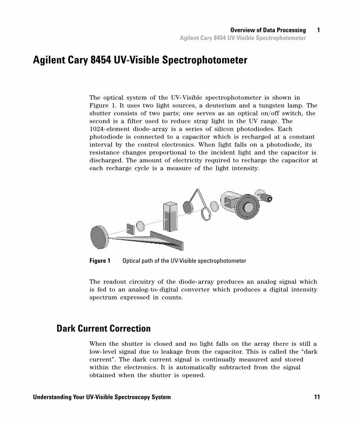
The optical system of the UV-Visible spectrophotometer is shown in Figure 1. It uses two light sources, a deuterium and a tungsten lamp. The shutter consists of two parts; one serves as an optical on/off switch, the second is a filter used to reduce stray light in the UV range. The 1024- element diode- array is a series of silicon photodiodes. Each photodiode is connected to a capacitor which is recharged at a constant interval by the control electronics. When light falls on a photodiode, its resistance changes proportional to the incident light and the capacitor is discharged. The amount of electricity required to recharge the capacitor at each recharge cycle is a measure of the light intensity.
The readout circuitry of the diode- array produces an analog signal which is fed to an analog- to- digital converter which produces a digital intensity spectrum expressed in counts.
Dark Current Correction
When the shutter is closed and no light falls on the array there is still a low- level signal due to leakage from the capacitor. This is called the “dark current”. The dark current signal is continually measured and stored within the electronics. It is automatically subtracted from the signal obtained when the shutter is opened.
Figure 1 Optical path of the UV-Visible spectrophotometer
Understanding Your UV-Visible Spectroscopy System 11
1 Overview of Data ProcessingAgilent Cary 8454 UV-Visible Spectrophotometer
Stray Light Correction
In a standard measurement sequence, reference or sample intensity spectra are measured both with and without the stray light filter in the light beam. Without the filter, the intensity spectrum over the whole wavelength range from 190- 1100 nm is measured. The stray light filter is a blocking filter with 50% blocking at 420 nm. With this filter in place, any light measured below 400 nm is stray light. This stray light intensity is then subtracted from the first spectrum to give a stray light corrected spectrum.
Variance
The read- out rate of the diode array is 100 msec. By means of the integration time, data can be acquired using multiples of the readout time. If an integration time greater than 100 msec is applied, multiple spectra, dependent upon the selected integration time, are acquired. An average spectrum is calculated and, if requested, variance data for each data are calculated in addition.
Reference Spectrum
The UV-Visible spectrophotometer is a single beam spectrophotometer. To generate a sample spectrum, two steps are required. First a “reference” intensity spectrum, I0, is measured. This is usually measured on the cuvette with solvent. This reference intensity spectrum is stored internally by the spectrophotometer.
Absorbance Spectra
For a sample, the intensity spectrum is measured and the absorbance spectrum is calculated (no stray light correction) using:
where
A Is Isd– I0 I0d– log–=
12 Understanding Your UV-Visible Spectroscopy System
Overview of Data Processing 1Agilent Cary 8454 UV-Visible Spectrophotometer
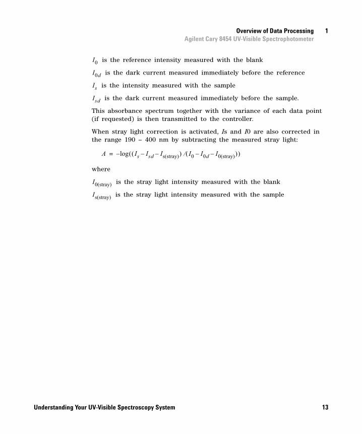
is the reference intensity measured with the blank
is the dark current measured immediately before the reference
is the intensity measured with the sample
is the dark current measured immediately before the sample.
This absorbance spectrum together with the variance of each data point (if requested) is then transmitted to the controller.
When stray light correction is activated, Is and I0 are also corrected in the range 190 – 400 nm by subtracting the measured stray light:
where
is the stray light intensity measured with the blank
is the stray light intensity measured with the sample
I0
I0d
Is
Isd
A Is Isd– Is(stray)– I0 I0d– I0(stray)– log–=
I0(stray)
Is(stray)
Understanding Your UV-Visible Spectroscopy System 13
1 Overview of Data ProcessingAgilent Cary 8454 UV-Visible Spectrophotometer
Wavelength Calibration
The UV-Visible spectrophotometer has a nominal sampling interval of 1 diode every 0.9 nm. Each spectrograph is calibrated in the factory using a series of emission lines from deuterium, zinc, argon and mercury lamps to obtain a calibration curve that relates each diode to a particular wavelength. The calibration parameters of this curve are stored within the ROM memory of each spectrograph. On site, this calibration can be checked by using the two emission lines from the deuterium lamp. With the aid of the calibration parameters, the firmware of the spectrophotometer determines absorbance values at 1 nm intervals and these values are then sent to the controller.
Invalid Data
The spectrophotometer will invalidate a measured spectrum under certain circumstances. This means that the measured spectrum is considered to be so unreliable that it is not usable. In the spectrum sent to the controller, the absorbance values at wavelength which are invalidated are set to a special value which is recognized by the controller software and these values are not displayed. Invalid data are produced when the sample is much more transparent then the reference data of the previously acquired blank. This causes an A/D converter overflow.
14 Understanding Your UV-Visible Spectroscopy System
Overview of Data Processing 1Data Flow in the Agilent ChemStation
Data Flow in the Agilent ChemStation
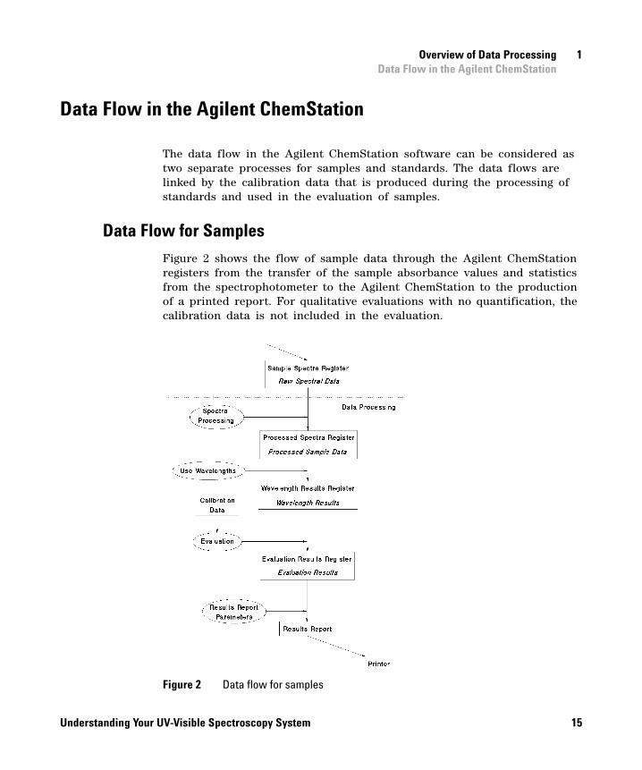
The data flow in the Agilent ChemStation software can be considered as two separate processes for samples and standards. The data flows are linked by the calibration data that is produced during the processing of standards and used in the evaluation of samples.
Data Flow for Samples
Figure 2 shows the flow of sample data through the Agilent ChemStation registers from the transfer of the sample absorbance values and statistics from the spectrophotometer to the Agilent ChemStation to the production of a printed report. For qualitative evaluations with no quantification, the calibration data is not included in the evaluation.
Figure 2 Data flow for samples
Understanding Your UV-Visible Spectroscopy System 15
1 Overview of Data ProcessingData Flow in the Agilent ChemStation
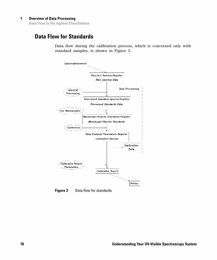
Data Flow for Standards
Data flow during the calibration process, which is concerned only with standard samples, is shown in Figure 3.
Figure 3 Data flow for standards
16 Understanding Your UV-Visible Spectroscopy System
Overview of Data Processing 1Data Flow in the Agilent ChemStation
The calibration coefficients that are calculated during the calibration process are stored with the data analysis parameters in the Data Analysis Parameters register as part of the current method.
Once a calibration has been performed, and the calibration coefficients have been added to the Data Analysis Parameters register, the quantitative evaluation procedure uses the stored calibration data to perform a quantitative analysis on all subsequent samples that are measured using the current method. No data is destroyed during any of the data processing operations.
Understanding Your UV-Visible Spectroscopy System 17
1 Overview of Data ProcessingData Flow in the Agilent ChemStation
18 Understanding Your UV-Visible Spectroscopy System

Agilent ChemStation for UV-Visible SpectroscopyUnderstanding Your UV-visible Spectroscopy System
2Agilent ChemStation Registers and Views
Registers 20
Views 24
19Agilent Technologies
2 Agilent ChemStation Registers and ViewsRegisters
Registers
A register is an area of computer memory where data is stored. The General Scanning software sets up several registers for different types of data; the most important registers are shown in Table 1.
Table 1 Agilent ChemStation Registers and Their Contents
Register Contents
Configuration System configuration data (see Chapter 8, “Configuration and Methods”)
Sample System Parameters
Sampling system parameters to be used for measurements
Spectrophotometer Parameters
Spectrophotometer measurement parameter
Blank Spectrum Last acquired blank spectrum
Raw Data(Sample Spectra)
Unprocessed data from sample measurements (usually absorbance data)
Raw Data(Standard Spectra)
Unprocessed data from standard sample measurements (usually absorbance data)
Math Result Results of interactive math processing
Method Description Definition of the method (see Chapter 8, “Configuration and Methods”)
Data Analysis Parameters Definitions and parameters of all data processing steps
ProcessedSample Spectra
Spectral data from samples after spectral processing
ProcessedStandard Spectra
Spectral data from standards after spectral processing
20 Understanding Your UV-Visible Spectroscopy System
Agilent ChemStation Registers and Views 2Registers
The registers that are specific to the standard samples and calibration data are used in the Quantification task only. During Quantification, the Data Analysis Parameters register includes the calibration coefficients generated during the calibration process.
In addition, registers are set up for instrument parameters, method and automation parameters and analysis results. Temporary registers are also set up during data processing and during the execution of tasks.
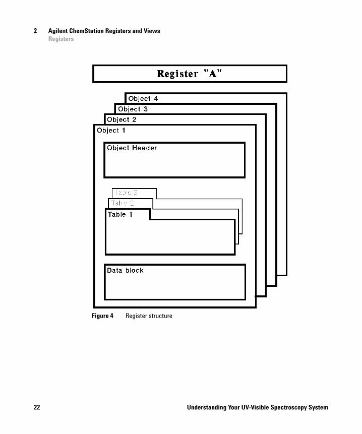
Structure and Contents of Registers
All registers have the same basic structure, which is similar to a database or card- index system. The fundamental unit of the register is the object, which is equivalent to a record in a database or a single card in a card index system. For example, a measured spectrum is an object in the raw data register. Each object has three parts:
• the object header, which contains static information about the object,
• a group of tables, which contain dynamic information about the object,
• the data block, which contains the object’s data.
A graphical representation of the structure of a register is shown in Figure 4 on page 22.
Wavelength Results Function results from the specified wavelengths of the sample spectra
Wavelength Results Standards
Function results from the specified wavelengths of the standard spectra
Evaluation Results Evaluation or analysis results
Evaluation Results Standards
Evaluation results that are used for calibration diagnostics
Table 1 Agilent ChemStation Registers and Their Contents (continued)
Register Contents
Understanding Your UV-Visible Spectroscopy System 21
2 Agilent ChemStation Registers and ViewsRegisters
Figure 4 Register structure
22 Understanding Your UV-Visible Spectroscopy System
Agilent ChemStation Registers and Views 2Registers
Data Structure of Spectra
The data structure of spectra is the same in the Samples register and the Math Result register:
• Header block, containing some or all of the following information:
Information about the sample:
• the sample name,
• solvent information (if available),
• any available comment,
• the operator name,
• the data type (absorbance).
Information about the instrument on which the sample was run:
• the identification of the type and firmware revision number,
• the instrument serial number.
Information about the acquisition:
• the date and time of acquisition,
• the integration time,
• the resolution,
• cell path length and units,
• cell temperature (if available).
• The Analytes Table, containing the information about the analytes. If no analyte information is available, this table is empty.
• The Data Block, containing the spectral information in a matrix of three rows:
• the wavelength in ascending order,
• the absorbance at that wavelength,
• the standard deviation of the measurement, calculated from the variance data transferred from the spectrophotometer.
Understanding Your UV-Visible Spectroscopy System 23
2 Agilent ChemStation Registers and ViewsViews
Views
Views are perspectives on the contents of registers. Each view displays the contents of the relevant registers in one or more windows; each window of the view displays a portion of the registers’ contents.
Relationship Between Views and Registers
The Samples view and Math view display the contents of the Processed Samples register and Math Result register respectively:
• The Sample Spectra window and Math Result window are graphical representations of the Data Blocks from the respective registers.
• The Sample/Result table of the Samples view contains selected information from the Header block, together with the evaluation results The Samples Table, accessible from the Sample/Result table, contains additional information from the Header block.
The Standards view displays the contents of the Processed Standard Spectra register.
24 Understanding Your UV-Visible Spectroscopy System

Agilent ChemStation for UV-Visible SpectroscopyUnderstanding Your UV-Visible Spectroscopy System
3Tasks
Fixed Wavelength Task 26
Spectrum/Peak 27
Ratio/Equation 28
Quantification 30
25Agilent Technologies
3 TasksFixed Wavelength Task
Fixed Wavelength Task
For details of the calculations used in this task, see Chapter 5, “Evaluation”.
The Fixed Wavelength task allows the calculation of results from up to six wavelengths with or without background correction. The Fixed Wavelength parameters are shown in Table 2:
Table 2 Parameters for the Fixed Wavelength Task
Parameter Data Flow Range of Values
Use Wavelength(s) Sets the Used Wavelengths (see “Use Wavelengths” on page 35) to the selected values.
Up to six single wavelengths
Background Correction Sets the Background Correction (see “Background Correction” on page 35) to the selected type.
nonesingle reference wavelengthsubtract average over a rangethree-point drop line
Data Type Sets the Spectral Processing (see “Spectral Processing” on page 34) to the selected type.
TransmittanceAbsorbanceDerivative 1Derivative 2Derivative 3Derivative 4
Display Spectrum Sets the upper and lower wavelength limits for spectral display.
Instrument Settings
26 Understanding Your UV-Visible Spectroscopy System
Tasks 3Spectrum/Peak
Spectrum/Peak
For details of the calculations used in this task, see Chapter 5, “Evaluation”.
The Spectrum/Peaks task determines the maxima and minima of the data points (y- values) in the defined wavelength range of the spectrum The last acquired spectrum is displayed annotated with the specified number of peaks and valleys, and the Sample Result table shows the wavelengths and absorbance values of the peaks and valleys. The All Peaks/Valleys button displays a list if the wavelengths and absorbencies of all peaks and valleys.
The original spectrum is first derivatized (see “Derivative” on page 60) using a filter length of 5 and a polynomial degree of 3. The derivatized y- values are examined for transitions (change of sign); each transitional y- value is compared with its neighboring values, and if the neighboring values are more extreme, the transitional y- value is compared with the previous transitional y- value. If the difference of both values is greater than or equal to the sensitivity threshold, then the previous transitional point is stored as an extremum; if the difference is less than the sensitivity threshold, then neither point is stored.
The Spectrum/Peaks parameters are shown in Table 3:
Table 3 Parameters for the Peak / Valley Find Task
Parameter Data Flow Range of Values
Data Type Sets the Spectral Processing (see “Spectral Processing” on page 34) to the selected type.
TransmittanceAbsorbanceDerivative 1Derivative 2Derivative 3Derivative 4
Display Spectrum Sets the upper and lower wavelength limits for spectral display
Instrument Settings
Number of Peaks Sets the number of peaks reported. 0 to 19
Number of Valleys Sets the number of valleys reported. 0 to 19
Understanding Your UV-Visible Spectroscopy System 27
3 TasksRatio/Equation
Ratio/Equation
For details of the calculations used in this task, see Chapter 5, “Evaluation”.
The Ratio/Equation task calculates a result based upon a specified equation. The equation can contain absorbencies from up to six wavelengths plus sample weight and volume information. The following mathematical operators are available for use in an equation:
The results of the equation are corrected for path length and dilution factor automatically.
The parameters for the Ratio/Equation task are shown in Table 4:
+ adds
- subtracts
/ divides
* multiplies
ABS(exp) returns the absolute value of the expression
Ceil(exp) rounds the expression up to the nearest integer
EXP(exp) returns
FLOOR(exp) rounds the expression down to the nearest integer
LN(exp) returns the natural logarithm (base e) of the expression
LOG(exp) returns the logarithm (base 10) of the expression
SQR(exp) returns the square of the expression
SQRT(exp) returns the square root of the expression
eexp
28 Understanding Your UV-Visible Spectroscopy System
Tasks 3Ratio/Equation
Table 4 Parameters for the Ratio/Equation Task
Parameter Data Flow Range of Values
Use Wavelength(s) Sets the Used Wavelengths (see “Use Wavelengths” on page 35) to the selected values.
Up to six single wavelengths
Data Type Sets the Spectral Processing (see “Spectral Processing” on page 34) to the selected type.
TransmittanceAbsorbanceDerivative 1Derivative 2Derivative 3Derivative 4
Equation Name Sets the equation name. Alphanumeric text
Equation Sets the equation parameters. Alphanumeric text
Unit Sets the units for the result. Alphanumeric text
Use sample weight and volume
Switches on the Weight and Volume entry fields in the Sample Information dialog box.
Checked (yes) or unchecked (no)
Prompt for sample information
Switches on the display of the Sample Information dialog box after sample measurement.
Checked (yes) or unchecked (no)
Display Spectrum Sets the upper and lower wavelength limits for spectral display
Instrument Settings
Understanding Your UV-Visible Spectroscopy System 29
3 TasksQuantification
Quantification
For details of the calculations used in this task, see Chapter 5, “Evaluation”.
The Quantification task calculates calibration coefficients from the measured data of a set of standards, then uses the calibration coefficients to determine the concentration of unknown samples. The equations used in the calculation of the calibration coefficients and the concentrations of unknown samples are given in Chapter 5, “Evaluation”. The parameters for the Quantification task are shown in Table 5:
Table 5 Parameters for the Quantification Task
Parameter Data Flow Range of Values
Use Wavelength Sets the Used Wavelengths (see “Data Transformation” on page 35) to the selected values.
Single wavelength value
Background Correction Sets the Background Correction (see “Background Correction” on page 35) to the selected type.
nonesingle reference wavelengthsubtract average over a rangethree-point drop line
Analyte name Sets the analyte name. Alphanumeric text
Calibration Curve Type Sets the calibration curve type (see “Calibration Curve Types” on page 42.)
linear (Beer’s law)linear with offsetquadraticquadratic with offset
Concentration unit Sets the units of concentration; when the Concentration option is chosen, switches on the Concentration entry field in the Sample Information dialog box.
alphanumeric text
Weight & Volume unit Sets the units of weight and volume; when the Weight & Volume option is chosen, switches on the Weight and Volume entry fields in the Sample Information dialog box.
alphanumeric text
30 Understanding Your UV-Visible Spectroscopy System
Tasks 3Quantification
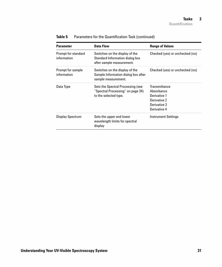
Prompt for standard information
Switches on the display of the Standard Information dialog box after sample measurement.
Checked (yes) or unchecked (no)
Prompt for sample information
Switches on the display of the Sample Information dialog box after sample measurement.
Checked (yes) or unchecked (no)
Data Type Sets the Spectral Processing (see “Spectral Processing” on page 34) to the selected type.
TransmittanceAbsorbanceDerivative 1Derivative 2Derivative 3Derivative 4
Display Spectrum Sets the upper and lower wavelength limits for spectral display
Instrument Settings
Table 5 Parameters for the Quantification Task (continued)
Parameter Data Flow Range of Values
Understanding Your UV-Visible Spectroscopy System 31
3 TasksQuantification
32 Understanding Your UV-Visible Spectroscopy System
Agilent ChemStation for UV-Visible SpectroscopyUnderstanding Your UV-Visible Spectroscopy System
4Spectral Processing and Data Transformation
Spectral Processing 34
Data Transformation 35
33Agilent Technologies
4 Spectral Processing and Data TransformationSpectral Processing
Spectral Processing
Absorbance
Absorbance is the default data type of spectral storage in the UV-Visible ChemStation.
Absorbance spectra are calculated using the Absorbance function; for a complete description of the mathematical processes involved in calculating absorbance spectra, see “Absorbance” on page 58.
Transmittance
Transmittance spectra are calculated using the Transmittance function; for a complete description of the mathematical processes involved in calculating transmittance spectra, see “Transmittance” on page 59.
Derivative
First, second, third and fourth order derivative spectra can be calculated. The Derivative functions calculate the derivative of the data points (y- values) in the spectrum to the specified derivative order using a Savitsky- Golay algorithm with a filter length of 5 and a polynomial degree of 3. For a complete description of the Derivative function, see “Derivative” on page 60.
34 Understanding Your UV-Visible Spectroscopy System
Spectral Processing and Data Transformation 4Data Transformation
Data Transformation
Use Wavelengths
The Use Wavelengths function selects a sub- set of data from the full spectrum. The sub- set may be the processed spectral intensity value at a single wavelength, as in the Quantification task, or the processed spectral intensity values at up to six wavelengths as in the Fixed Wavelengths and Ratio/Equation tasks. The extracted value(s) may then be subjected to further modification by background correction to produce the final result.
Background Correction
Background correction subtracts a calculated “background” value from the extracted spectral intensity value(s). There are three methods of calculating the background values:
• single reference wavelength
• subtract average over a range
• three- point drop line, used when two wavelengths are set
Single Reference Wavelength
The single reference wavelength method subtracts the spectral intensity value at a specified wavelength, as in Figure 5 on page 36. The reference wavelength is usually selected at a point on the baseline beyond the sample absorbance.
Understanding Your UV-Visible Spectroscopy System 35
4 Spectral Processing and Data TransformationData Transformation
Subtraction is carried out using Equation 1:
(1)
where
f is the function result at wavelength
A is the absorbance at wavelength
AR is the absorbance at reference wavelength
The variances (if available) are treated according to Equation 2:
(2)
where
var(f) is the variance of the function result at wavelength
var(A)is the variance of the absorbance at wavelength
var(AR)is the variance of the absorbance at reference wavelength
Figure 5 Background correction to a single reference wavelength
f A AR–=
var f var A var AR +=
36 Understanding Your UV-Visible Spectroscopy System
Spectral Processing and Data Transformation 4Data Transformation
Subtract Average Over Range
The subtract average over range method uses the same calculation as for a single reference wavelength (see “Single Reference Wavelength” on page 35), but replaces the spectral intensity value at the single wavelength with the average intensity value over a specified wavelength range.
where the terms are the same as for a single reference wavelength (see “Background Correction” on page 35).
Three-Point Drop Line
For a three- point drop- line background correction, the spectral intensity and variance values from two reference wavelengths are taken, giving ,
, and . In this case, the reference wavelengths define a
straight line (as in Figure 6 on page 38) which is used to calculate and using Equation 3 and Equation 4.
(3)
(4)
where the terms are the same as for a single reference wavelength (see “Background Correction” on page 35). In Figure 6 on page 38, the upper trace shows the spectrum before background correction, with the three- point drop line superimposed. The lower trace shows the spectrum after background correction.
f A=AR1
A+R2
AR3 ARn
+ + +
n---------------------------------------------------------------------- –
AR1
AR2var AR1
var AR2
ARvar AR
AR
1R2
R1–
---------------------- R2– AR1
R1– AR2
+ =
var AR 1
R2R1
– 2----------------------------- R2
– 2var AR1 R1
– 2var AR2 +
=
Understanding Your UV-Visible Spectroscopy System 37
4 Spectral Processing and Data TransformationData Transformation
Figure 6 Three-point drop line
38 Understanding Your UV-Visible Spectroscopy System
Agilent ChemStation for UV-Visible SpectroscopyUnderstanding Your UV-Visible Spectroscopy System
5Evaluation
Evaluation using an Equation 40
Quantification 41
This chapter describes the use of equations, and introduces quantification and explains the concepts that are used in the Quantification task of the software. It also describes the mathematical and statistical calculations that are used to produce a calibration curve for single component analysis and how the quantitative results are calculated using the calibration data.
39Agilent Technologies
5 EvaluationEvaluation using an Equation
Evaluation using an Equation
When an equation evaluation is specified, the analysis results are the results of the equation specified in the Equation Parameter dialog box. In the definition of the equation, you can use any result generated by the Use Wavelength(s) and stored in the Wavelength Results register and any of the other predefined variables: Dilution factor, Weight and Volume.
By default, the results are normalized to a 1 cm path length by dividing the function result by the value of the Path Length parameter in the Sample Spectra table:
(5)
where
fcorr is the function result after path length correction
f is the uncorrected function result
l is the path length
fcorrfl-=
40 Understanding Your UV-Visible Spectroscopy System
Evaluation 5Quantification
Quantification
The Quantification task of the Agilent ChemStation software includes facilities for:
• measurement of calibration standards,
• calibration of a single analyte using the calibration standards,
• measurement of unknown samples, and
• quantification of the analyte in the unknown samples.
Beer-Lambert Law
The Beer- Lambert law states that the absorbance of a solute is directly proportional to its concentration:
(6)
In Equation 6:
A is absorbance
E is molar absorptivity or molar extinction coefficient (l.mol- 1.cm- 1)
c is analyte concentration (mol.l- 1)
d is cell path length (cm)
To calculate the concentration of an unknown compound, the above equation can be solved for a given function result, f:
(7)
The reciprocal of the product of molar extinction coefficient and cell path length is often called the calibration coefficient, k.
(8)
A Ecd=
cf
Ed-------=
c kf=
Understanding Your UV-Visible Spectroscopy System 41
5 EvaluationQuantification
Calibration
Calibration is the correlation of the function result with known concentrations of sample. The basic assumption is that the variance in the measured data is less than the variance in the standard concentrations. As a result of this correlation a calibration curve can be fitted to the data points and calibration coefficients can be calculated. The concentrations of unknown samples can then be calculated from the calibration coefficients and the function result of the samples.
Calibration Curve Types
Real data may deviate slightly from the ideal linear relationship described in “Beer- Lambert Law” on page 41. The relationship between the function result and concentration may be described more accurately by adding an offset (a non- zero intercept) or a quadratic term (or both) to the equation.
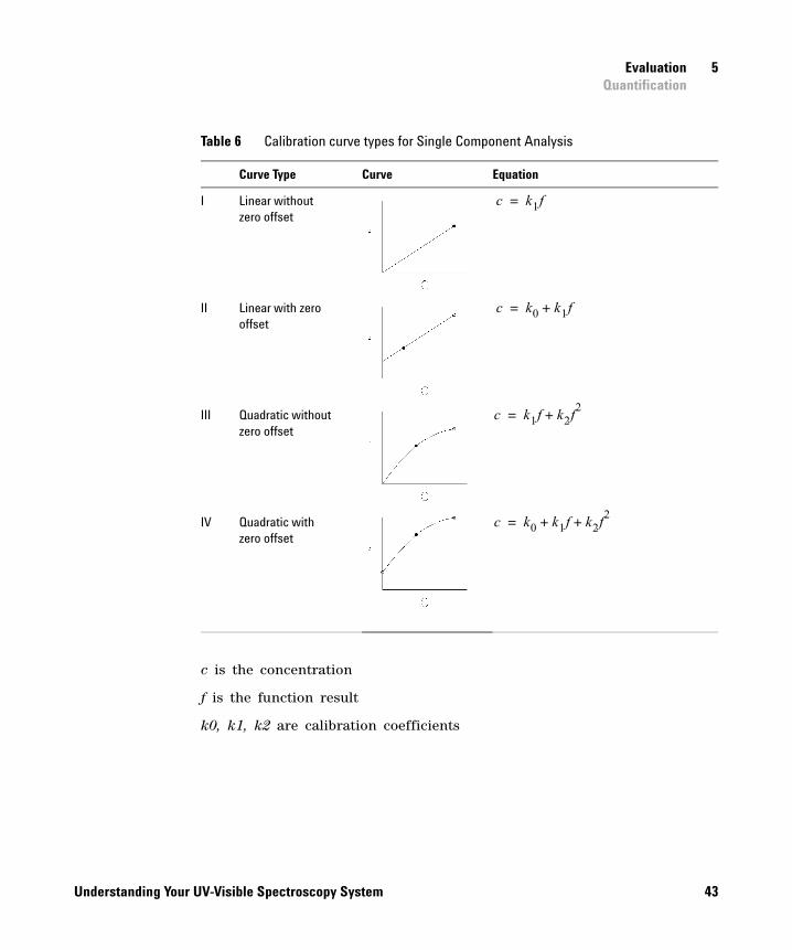
The ChemStation provides four different calibration curve types, shown in Table 6. These calibration curve graphs are shown in the more traditional way with the concentration on the x- axes and the function results on the y- axes.
The Agilent ChemStation provides four different calibration curve types, shown in Table 6.
42 Understanding Your UV-Visible Spectroscopy System
Evaluation 5Quantification
c is the concentration
f is the function result
k0, k1, k2 are calibration coefficients
Table 6 Calibration curve types for Single Component Analysis
Curve Type Curve Equation
I Linear without zero offset
II Linear with zero offset
III Quadratic without zero offset
IV Quadratic with zero offset
c k1f=
c k0 k1f+=
c k1f k2f2
+=
c k0 k1f k2f2
+ +=
Understanding Your UV-Visible Spectroscopy System 43
5 EvaluationQuantification
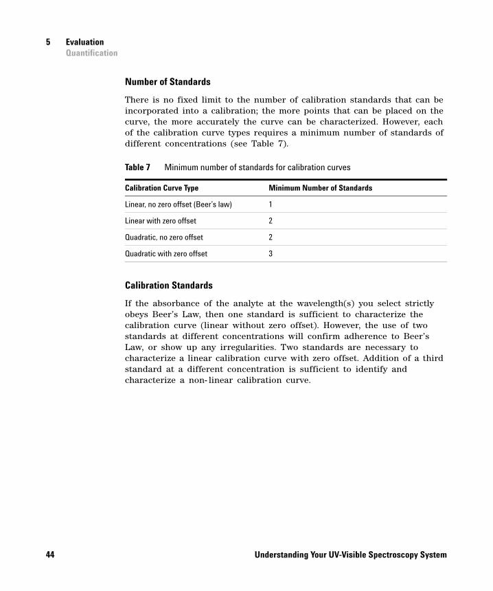
Number of Standards
There is no fixed limit to the number of calibration standards that can be incorporated into a calibration; the more points that can be placed on the curve, the more accurately the curve can be characterized. However, each of the calibration curve types requires a minimum number of standards of different concentrations (see Table 7).
Calibration Standards
If the absorbance of the analyte at the wavelength(s) you select strictly obeys Beer’s Law, then one standard is sufficient to characterize the calibration curve (linear without zero offset). However, the use of two standards at different concentrations will confirm adherence to Beer’s Law, or show up any irregularities. Two standards are necessary to characterize a linear calibration curve with zero offset. Addition of a third standard at a different concentration is sufficient to identify and characterize a non- linear calibration curve.
Table 7 Minimum number of standards for calibration curves
Calibration Curve Type Minimum Number of Standards
Linear, no zero offset (Beer’s law) 1
Linear with zero offset 2
Quadratic, no zero offset 2
Quadratic with zero offset 3
44 Understanding Your UV-Visible Spectroscopy System
Evaluation 5Quantification
Calibration Curve Fits
The mathematical problem is to find the calibration coefficients in a given curve type which will allow the best determination of a future unknown sample.
The least squares method uses the analytical function data from Use Wavelengths of all standards to determine the calibration coefficients of the chosen calibration curve type by a least squares calculation.
If each ith data set of the n standard data sets is expected to obey a function in the p coefficients, kj, although the real (measured) values may cluster around the function because of statistical errors, i, then the general equation is:
(9)
where
i is 1, 2, 3, … n (the total number of standards)
The calibration coefficients, kj, can be estimated using the least squares method, that is minimizing the sum of the squares of the errors, i (the differences between the measured value and the calibration curve).
(10)
In matrix notation:
(11)
where
C is n- concentration column vector
F is n p function result data matrix
k is p- calibration coefficient column vector
is n- error column vector
The elements used in the calibration matrix F and the coefficient vector k are given in Table 8 on page 46 with dimension p of the coefficient vector.
fi ci( , )
ci k0 k1fi k2fi2 i+ + +=
cactualiccalculatedi
– 2
i 1=
n
i2
i 1=
n
minimum= =
C Fk +=
Understanding Your UV-Visible Spectroscopy System 45
5 EvaluationQuantification
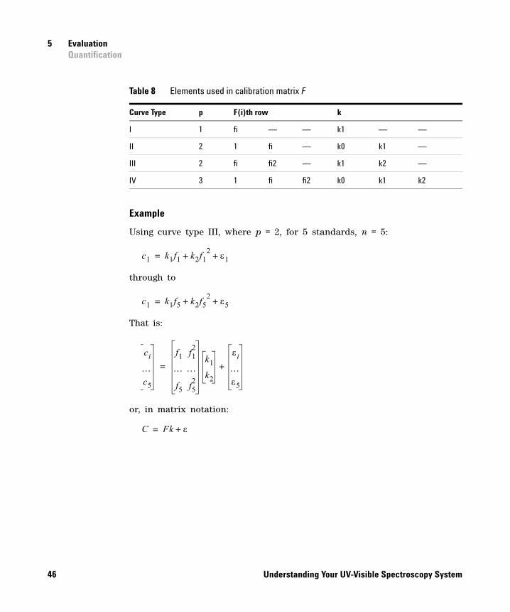
Example
Using curve type III, where p = 2, for 5 standards, n = 5:
through to
That is:
or, in matrix notation:
Table 8 Elements used in calibration matrix F
Curve Type p F(i)th row k
I 1 fi — — k1 — —
II 2 1 fi — k0 k1 —
III 2 fi fi2 — k1 k2 —
IV 3 1 fi fi2 k0 k1 k2
c1 k1f1 k2f12 1+ +=
c1 k1f5 k2f52 5+ +=
ci
c5
f1 f12
f5 f52
k1
k2
i
5
+=
C Fk +=
46 Understanding Your UV-Visible Spectroscopy System
Evaluation 5Quantification
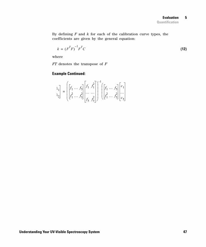
By defining F and k for each of the calibration curve types, the coefficients are given by the general equation:
(12)
where
FT denotes the transpose of F
Example Continued:
k FT
F 1–F
TC=
k1
k2
f1 f5
f12 f5
2
f1 f12
f5 f52
1–
f1 f5
f12 f5
2
c1
c5
=
Understanding Your UV-Visible Spectroscopy System 47
5 EvaluationQuantification
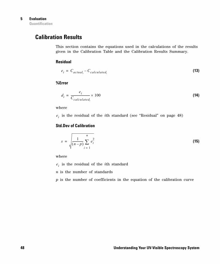
Calibration Results
This section contains the equations used in the calculations of the results given in the Calibration Table and the Calibration Results Summary.
Residual
(13)
%Error
(14)
where
is the residual of the ith standard (see “Residual” on page 48)
Std.Dev of Calibration
(15)
where
is the residual of the ith standard
n is the number of standards
p is the number of coefficients in the equation of the calibration curve
ei CactualiCcalculatedi
–=
di
ei
Ccalculatedi
---------------------------- 100=
ei
s1
n p– ---------------- ei
2
i 1=
n
=
ei
48 Understanding Your UV-Visible Spectroscopy System
Evaluation 5Quantification
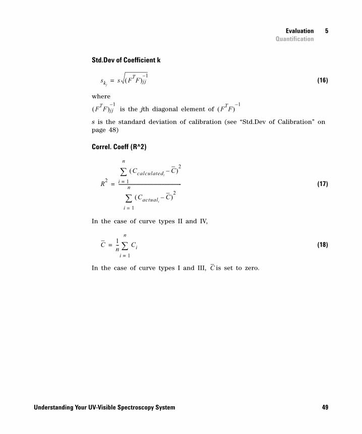
Std.Dev of Coefficient k
(16)
where
is the jth diagonal element of
s is the standard deviation of calibration (see “Std.Dev of Calibration” on page 48)
Correl. Coeff (R^2)
(17)
In the case of curve types II and IV,
(18)
In the case of curve types I and III, is set to zero.
skjs F
TF jj
1–=
FT
F jj1–
FT
F 1–
R2
CcalculatediC–
2
i 1=
n
CactualiC–
2
i 1=
n
--------------------------------------------------------=
C1n--- Ci
i 1=
n
=
C
Understanding Your UV-Visible Spectroscopy System 49
5 EvaluationQuantification
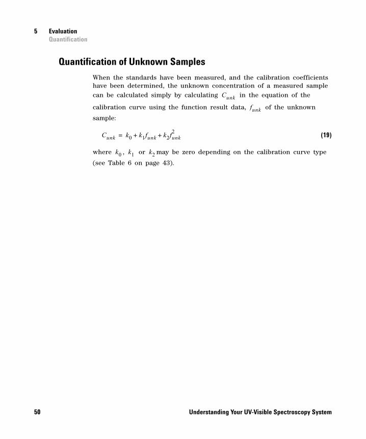
Quantification of Unknown Samples
When the standards have been measured, and the calibration coefficients have been determined, the unknown concentration of a measured sample can be calculated simply by calculating in the equation of the
calibration curve using the function result data, of the unknown
sample:
(19)
where , or may be zero depending on the calibration curve type
(see Table 6 on page 43).
Cunk
funk
Cunk k0 k1funk k2funk2
+ +=
k0 k1 k2
50 Understanding Your UV-Visible Spectroscopy System
Agilent ChemStation for UV-Visible SpectroscopyUnderstanding Your UV-Visible Spectroscopy System
6Reports
Method Report 53
Results Report 55
Automation Reports 56
The general purpose UV-Visible software for the Agilent ChemStation allows four reports to be generated.
• The Method Report is a report of the parameters of the current method.
• The Results Report is a report of the current evaluation results.
• The Automation Method Report is a report of the parameters of the current Automation Table.
• The Automation Results Report is a report of the current automation results.
The reports can be output directly to a printer or printed as a text file to a file with the extension .TXT. Reports that are printed to files are stored in the REPORTS subdirectory of the instrument’s subdirectory.
In addition to the two formal reports, the UV-Visible ChemStation software allows any selected window to be printed, and any view (all windows) to be printed. The windows and views are formatted as reports.
51Agilent Technologies
6 Reports
The appearance of the report is affected by two sets of parameters:
• The report configuration parameters control the margins, and indents for textual data. The annotation limit, which is the maximum number of spectra that are annotated, is also controlled by the report configuration parameters. If a spectrum plot contains less spectra than the annotation limit, all spectra are annotated. If the spectrum plot contains more spectra than the annotation limit, none of the spectra are annotated.
• The printer setup parameters control the target printer and the paper size and orientation.
The title of the report contains the task name together with the date and time of generation.
52 Understanding Your UV-Visible Spectroscopy System
Reports 6Method Report
Method Report
The method report contains the information and parameters of the current method:
The Spectrophotometer parameters are extracted from the Instrument Parameters dialog box:
Method file The method file name.
Information The contents of the Method Information field of the Method Options and Information dialog box.
Operator The Operator Name when the method was set up or modified.
Product The Agilent ChemStation.
Instrument The name of the instrument, from the configuration file.
Acquisition range The instrument acquisition range from the Instrument Parameters dialog box.
Integration Time The instrument integration time from the Instrument Parameters dialog box.
Std Deviation Standard deviation is always Off.
Understanding Your UV-Visible Spectroscopy System 53
6 ReportsMethod Report
The Data Analysis parameters are extracted from the parameters dialog box for the current task; some of the parameters reported depend on the task:
Data Type (All Tasks) The data type from the parameters dialog box for the current task.
Display spectrum (All Tasks) The limits of spectral display from the parameters dialog box for the current task.
Used Wavelength (Fixed Wavelength and Quantification) The contents of the Used Wavelength(s) field(s) of the parameters dialog box for the current task.
Background Correction (Fixed Wavelength and Quantification) The contents of the Background Correction field(s) of the parameters dialog box for the current task.
Find up to (Spectrum/Peaks) Two lines showing the selected number of peaks and valleys taken from the Spectrum/Peaks Parameters dialog box.
Equation (Ratio/Equation) The name and formula of the equation from the Equation Parameters dialog box.
Where (Ratio/Equation) The explanation of the terms of the equation.
54 Understanding Your UV-Visible Spectroscopy System
Reports 6Results Report
Results Report
The results report contains a header section with information about the method and data files, a graphical section and a results table. The graphical section and results table correspond with the Samples view for the selected task.
The header information consists of:
In addition, the Results report for the Quantification task includes a summary of the calibration results:
The last line of the report contains the current operator’s name and a space for the operator’s signature.
Method file The method file name.
Information The contents of the Method Information field of the Method Options and Information dialog box.
Data File The data file name (including the full path name) and the date and time of creation.
Analyte name The analyte name taken from the Quantification Parameters dialog box.
Calibration equation The calibration equation calculated using the selected calibration curve type from the spectral data values extracted from the standard spectra.
Calibrated at The date, time and operator name when the calibration was performed.
Understanding Your UV-Visible Spectroscopy System 55
6 ReportsAutomation Reports
Automation Reports
The automation reports comprise an Automation Method report and an Automation Results Report.
Automation Method Report
The automation method report is a summary of the Automation Table. It contains the following information:
Automation Results Report
The automation results report contains an appropriate Results Report (see “Results Report” on page 55) for each sample in the automated sequence. In addition, statistics of the sample results can be calculated:
• average value,
• minimum value,
• maximum value,
• standard deviation,
• % relative standard deviation.
Operator The name of the automation operator.
Method file The automation method file name.
Measure Blank The blank measurement sequence, taken from the Automation Setup dialog box.
Measure Standard The standards and their concentrations, taken from the Automation Setup dialog box.
Measure Control The control samples, their concentrations and the maximum permitted error, taken from the Automation Setup dialog box.
Measure Samples The seed name of the samples, the number of samples and their dilution factor, taken from the Automation Setup dialog box.
Measurement sequence The measurement sequence table, equivalent to the Automation Measurement Sequence dialog box.
56 Understanding Your UV-Visible Spectroscopy System
Agilent ChemStation for UV-Visible SpectroscopyUnderstanding Your UV-Visible Spectroscopy System
7Interactive Math Functions
Unitary Operations 58
Binary Operations 64
57Agilent Technologies
7 Interactive Math FunctionsUnitary Operations
Unitary Operations
The unitary mathematical functions operate on single spectra. If more than one spectrum is selected, the function operates on all selected spectra individually. If no spectra are selected, the operation is aborted and an error message is displayed.
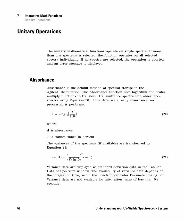
Absorbance
Absorbance is the default method of spectral storage in the Agilent ChemStation. The Absorbance function uses logarithm and scalar multiply functions to transform transmittance spectra into absorbance spectra using Equation 20. If the data are already absorbance, no processing is performed.
(20)
where
A is absorbance
T is transmittance in percent
The variances of the spectrum (if available) are transformed by Equation 21:
(21)
Variance data are displayed as standard deviation data in the Tabular Data of Spectrum window. The availability of variance data depends on the integration time, set in the Spectrophotometer Parameter dialog box. Variance data are not available for integration times of less than 0.2 seconds .
A log10T
100--------- –=
var A 1T 10ln------------------- 2
var T =
58 Understanding Your UV-Visible Spectroscopy System
Interactive Math Functions 7Unitary Operations
Transmittance
The Transmittance function uses exponential, reciprocal and scalar multiply functions to transform absorbance spectra into transmittance spectra using Equation 22. The transmittance spectra are placed in the math result register.
(22)
The variances, if available, are transformed by Equation 23:
(23)
All additional information, such as annotations, are preserved unchanged in the transmittance spectrum.
T 100 10A–=
var T 100 ln10 10A–
2var A =
Understanding Your UV-Visible Spectroscopy System 59
7 Interactive Math FunctionsUnitary Operations
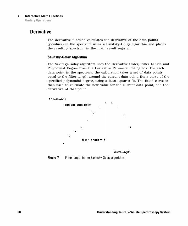
Derivative
The derivative function calculates the derivative of the data points (y- values) in the spectrum using a Savitsky- Golay algorithm and places the resulting spectrum in the math result register.
Savitsky-Golay Algorithm
The Savitsky- Golay algorithm uses the Derivative Order, Filter Length and Polynomial Degree from the Derivative Parameter dialog box. For each data point in the spectrum, the calculation takes a set of data points equal to the filter length around the current data point, fits a curve of the specified polynomial degree, using a least squares fit. The fitted curve is then used to calculate the new value for the current data point, and the derivative of that point:
Figure 7 Filter length in the Savitsky-Golay algorithm
60 Understanding Your UV-Visible Spectroscopy System
Interactive Math Functions 7Unitary Operations
For each y- value, yi,
(24)
where
i is 1 … data points- (filter length- 1)
j is 1 … filter length
k is 1 for smoothing, 2 for derivative
deriv(y1) corresponds to the th value. For example, if
filter length is 5, then deriv(y1) becomes y3. For this reason, the length of the spectrum is reduced by (filter length - 1) values;
values at the beginning of the spectrum and
values at the end of the spectrum are not processed. In
Equation 24, C is the coefficient matrix:
(25)
where
N- 1 is the inverse of N, the product of FT and F
FT is the transpose of F, the matrix of the powers of the polynomials
The matrix of the powers of the polynomials is generated using Equation 26:
(26)
where
i is 1 … filter length
j is 1… degree +1
k is
deriv yi Ckj yi j 1–+=
filter length-1 2
-------------------------------------- 1+
filter length-1 2
--------------------------------------
filter length-1 2
--------------------------------------
C N1–
FT=
Fij kj 1–
=
ifilter length 1–
2------------------------------------- 1––
Understanding Your UV-Visible Spectroscopy System 61
7 Interactive Math FunctionsUnitary Operations
The y- values are multiplied by the reciprocal of the wavelength step at the end of the calculation:
(27)
where
step is the increment of the equidistant x- axis
For each variance value, var(yi),
(28)
where
C is the coefficient matrix
i is 1 … data points - (filter length - 1)
j is 1 … filter length
k is 1 for smoothing, 2 for derivative
The variance values are multiplied by the square of the reciprocal of the step at the end of the calculation:
(29)
If one of the values needed for the calculation is invalid, the resulting y- value or variance value is invalid.
All additional information, such as annotations, are preserved unchanged in the derivative spectrum.
yi
yi
step---------=
deriv var yi Ckj2
var yi j 1–+ =
var yi var yi
step2
-----------------=
62 Understanding Your UV-Visible Spectroscopy System
Interactive Math Functions 7Unitary Operations
Scalar Add
The scalar add function adds a constant value to each of the data points (y- values) in the spectrum and places the resulting spectrum in the math result register.
(30)
The scalar add function can be used to subtract a constant value by using a negative constant.
The variances (if available) and all other additional information, such as annotations, are preserved unchanged in the resulting spectrum.
Scalar Multiply
The scalar multiply function multiplies each of the data points (y- values) in the spectrum by constant value and places the resulting spectrum in the math result register.
(31)
The scalar multiply function can be used to divide by a constant value by
using the reciprocal of the desired divisor, .
The variances (if available) are multiplied by the square of the constant value:
(32)
All other additional information, such as annotations, are preserved unchanged in the resulting spectrum.
ynew y C+=
ynew y C=
1C----
var ynew var y C2=
Understanding Your UV-Visible Spectroscopy System 63
7 Interactive Math FunctionsBinary Operations
Binary Operations
The binary mathematical functions, add and subtract, require two spectra for their operation. If no spectra are selected, or more than two spectra are selected, the operation is aborted and an error message is displayed.
Add
The add function adds two spectra together and places the result in the math result register. The spectrum selected first (spectrum A) is taken as the model and provides the wavelength range and resolution for the resulting spectrum. Spectrum A is first copied into the math result register, then the y- values (for example absorbance) from the second selected spectrum (spectrum B) are added to the y- values of the spectrum in the math result register as follows:
Spectra of Different Wavelength Resolutions
If the x- values of spectrum A do not completely agree with those of spectrum B
• the y- values of spectrum B are interpolated before adding them to the y- values of the resulting spectrum when the interval of the x- value in spectrum A is less than that of spectrum B.
• the y- values at intermediate x- values in spectrum B are ignored when the interval of the x- value of spectrum A is greater than that of spectrum B, and only the y- values from spectrum B at the x- values corresponding to spectrum A are added to the y- values of the resulting spectrum.
64 Understanding Your UV-Visible Spectroscopy System
Interactive Math Functions 7Binary Operations
Spectra of Different Wavelength Ranges
If the x- range (wavelength range) of spectrum A is greater than the x- range of spectrum B, the extra y- values in spectrum A remain unchanged in the result.
If the x- range of spectrum A is less than the x- range of spectrum B, the extra y- values in spectrum B are ignored.
If there is no overlap between the x- ranges of the spectra, spectrum A remains unchanged.
Variances
If variances are available in both spectra, the values from the spectrum B are added to those in spectrum A in the same way as for the y- values.
If only spectrum A contains variances, the values remain unchanged in the result.
If only spectrum B has variances, they are ignored.
Additional information, such as annotations, are taken solely from spectrum A; all such items from spectrum B are ignored.
Subtract
The subtract function subtracts one spectrum from another and places the result in the math result register. The spectrum selected first (spectrum A) is taken as the model and provides the wavelength range and resolution for the resulting spectrum. Spectrum A is first copied into the math result register, then the y- values (for example absorbance) from the second selected spectrum (spectrum B) are subtracted from the y- values of the spectrum in the math result register as follows.
Spectra of Different Wavelength Resolutions
If the x- values of spectrum A do not completely agree with those of spectrum B:
• the y- values of spectrum B are interpolated before subtracting them from the y- values of the resulting spectrum when the interval of the x- value in spectrum A is less than that of spectrum B, and
Understanding Your UV-Visible Spectroscopy System 65
7 Interactive Math FunctionsBinary Operations
• the y- values at intermediate x- values in spectrum B are ignored when the interval of the x- value of spectrum A is greater than that of spectrum B, and only the y- values from spectrum B at the x- values corresponding to spectrum A are subtracted from the y- values of the resulting spectrum.
Spectra of Different Wavelength Ranges
If the x- range (wavelength range) of spectrum A is greater than the x- range of spectrum B, the extra y- values in spectrum A remain unchanged in the result.
If the x- range of spectrum A is less than the x- range of spectrum B, the extra y- values in spectrum B are ignored.
Variances
If variances are available in both spectra, the values from the spectrum B are added to those in spectrum A in the same way as for the Add function (see “Add” on page 64).
If only spectrum A contains variances, the values remain unchanged in the result.
If only spectrum B has variances, they are ignored.
Additional information, such as annotations, are taken solely from spectrum A; all such items from spectrum B are ignored.
66 Understanding Your UV-Visible Spectroscopy System
Agilent ChemStation for UV-Visible SpectroscopyUnderstanding Your UV-Visible Spectroscopy System
8Configuration and Methods
System Configuration 68
The Configuration File 70
Methods 71
The ChemStation.ini File 75
The Directory Structure 76
67Agilent Technologies
8 Configuration and MethodsSystem Configuration
System Configuration
The configuration of the PC hardware and the Agilent ChemStation software to communicate with the UV-Visible spectrophotometer and its accessories requires the following steps:
• Configuration of the communications between the Agilent ChemStation and the other devices (spectrophotometer, temperature controller) that are connected with and controlled by it. This process is carried out using the Configuration Editor.
• Internal configuration of the software using the commands from the Config menu.
• Configuration of the sampling system using the commands from the Instrument menu.
Configuring the Hardware
The Configuration Editor, which is a stand- alone program, is used to configure the Agilent ChemStation for the spectrophotometers and other GPIB accessories that are connected with it. The Configuration Editor sets up the communication pathways that allow the Agilent ChemStation to control the spectrophotometer and other accessories that communicate via GPIB or LAN. The Configuration Editor builds the configuration information into the ChemStation.ini file located in the windows directory of your Microsoft® Windows™ operating system installation.
The Editor is also used to configure the UV- Visible ChemStation software’s color scheme, and can be used to define the default paths for the Agilent ChemStation software’s files; configuration information for both the color scheme and paths are also included in the ChemStation.ini file.
NOTE You can also redefine paths for the data files, method files and automation files (automation table and sample table) from within the Agilent UV-Visible ChemStation software
68 Understanding Your UV-Visible Spectroscopy System
Configuration and Methods 8System Configuration
The UV-Visible spectrophotometer and Agilent ChemStation undergo a dialog during start- up that results in the automatic configuration of the spectrophotometer. The following information is passed from the spectrophotometer to the Agilent ChemStation:
• The instrument type, firmware revision number and serial number
• The sampling interval
• The time for which the instrument has been switched on.
• The lamp condition (on or off)
• The spectrophotometer status
• The availability of a blank spectrum
The Agilent ChemStation downloads the spectrophotometer parameters of the current method to the spectrophotometer when the method is loaded during start- up.
Understanding Your UV-Visible Spectroscopy System 69
8 Configuration and MethodsThe Configuration File
The Configuration File
The configuration file controls the system set- up at start- up. All information relating to the configuration of the Agilent ChemStation software is stored in the configuration file, and the information is transferred into the configuration register when the Agilent ChemStation is started. The file is updated (and the current configuration saved) by overwriting the current contents of the file with the contents of the configuration register when the Save Configuration check box is selected when the Agilent ChemStation software is closed down.
When you save the configuration using the Save Configuration check box, you also save the current size and position of all windows and tables in all views.
The configuration register contains the following information:
User interface parameters Definitions of the sizes and positions of all graphics windows.
Table templates and descriptions
Definitions of the format and contents of all tables.
System variables
The current sample name, whether the method has changed or not, system messages: information and error messages.
Acquisition information Information about sampling systems, and the Configuration of Verification table.
Report information
Information for the formatting of reports.
70 Understanding Your UV-Visible Spectroscopy System
Configuration and Methods 8Methods
Methods
A method is a set of parameters that defines the analysis of a sample. A method can define a simple analysis, such as measuring the sample in the cell and displaying the absorbance spectrum, or a complex one, such as introducing a sample using the specified sampling system, measuring the sample, performing spectral processing steps, calculating a result using a pre- defined equation and printing a report.
The Structure of Methods
The method definition optionally includes any or all of the following parameters:
• a description of the method.
• instrument and acquisition parameters:
• parameters to prepare the configured sampling system to collect the sample.
• the sample temperature and stirrer parameters of the Agilent 89090A temperature controller (if fitted and configured).
• the acquisition parameters of the spectrophotometer.
• the name of the data file in which the measured spectra will be stored automatically.
• the parameters for the user interface display.
• the data analysis parameters:
• the spectral processing parameters that are applied to the measured spectra.
• parameters for the extraction of wavelength data.
• the parameters necessary for the calculation of the final result, for example an equation or quantification parameters, depending on the method.
The contents of the method definition depends on the settings defined by the user and the functionality available in the selected task.
Understanding Your UV-Visible Spectroscopy System 71
8 Configuration and MethodsMethods
Method Files
Method files are stored in a subdirectory METHODS of the instrument directory (1 for example). They have the extension .M.
The Status of Methods
Methods can exist in two states:
• as the current method, which is the method that is loaded into memory,
• as a stored method on disk. The current method can be stored on disk by selecting Save Method As from the File menu. Any stored method can replace the current method in memory by selecting Load Method…from the File menu and specifying the method to be loaded.
The Contents of the Method
The definition of the current method is held in a register (see “Registers” on page 20 for a description of registers), which contains the following information:
• the date and time of the last update of the method.
• the product number and software revision number.
• the contents of the Method Information field of the Method Options and Information dialog box.
• The state of the Autosave Spectra to File check box and the contents of the adjacent field in the Method Options and Information dialog box.
• a table that is the core of the method containing the information that defines the method parameters:
• data analysis parameters,
• spectrophotometer parameters,
• temperature controller parameters,
• sampling system parameters,
• report parameters,
• automation parameters.
72 Understanding Your UV-Visible Spectroscopy System
Configuration and Methods 8Methods
On Using a Method
When a method is loaded, the system is set up using the method parameters. The Measure command causes the method to be executed. On Using a Method shows the processes that occur, and the information that is input at each stage when a complete method is executed.
Sample Measurement
1 The configured sampling system collects the sample with the conditions specified in its parameter dialog box.
2 If the Wait for Temperature Ready check box in the sampling system’s Setup dialog box is selected, the Agilent ChemStation checks the status of the Agilent 89090A Peltier temperature control accessory.
3 When the status of the temperature controller is Ready, the Agilent ChemStation initiates a measurement by the spectrophotometer of the sample in the cell using the parameters specified in the Spectrophotometer Parameters dialog box.
4 If the method is used in an Automation, and the Autosave Spectra to File check box in the Method Options and Information is selected, the spectra are appended to the defined file.
Data Analysis
1 The measured spectra undergo data analysis.
The sample spectra are processed using the parameters defined in the parameters dialog box for the selected task.
The data for the wavelength results are extracted from the processed spectra and the wavelength result is calculated.
If the Ratio/Equation task has been selected, the analysis result is calculated from the wavelength result using the equation parameters.
If the Quantification task has been selected, the analysis result is calculated from the wavelength result using the quantification parameters.
Understanding Your UV-Visible Spectroscopy System 73
8 Configuration and MethodsMethods
Printing the Report
1 The report is formatted according to the parameters in the Configure Report dialog box and printed according to the parameters in the Printer Control dialog box.
74 Understanding Your UV-Visible Spectroscopy System
Configuration and Methods 8The ChemStation.ini File
The ChemStation.ini File
During installation of the software and configuration of the system, three or more sections are added to the ChemStation.ini file:
[PCS] contains the information about the instruments that are connected and the communications parameters.
[PCS,n] contains the details of screen colors, data paths and file names for instrument number n. Each configured spectrophotometer has an entry, for example [PCS,1], [PCS,2] and so on.
[HPCHEM] contains the access level and the encrypted password.
CAUTION You must not change any of the entries in these sections of the ChemStation.ini file. Any changes will give rise to unpredictable behavior, and may prevent the UV-Visible ChemStation software from starting up.
Understanding Your UV-Visible Spectroscopy System 75
8 Configuration and MethodsThe Directory Structure
The Directory Structure
During installation of the Agilent ChemStation software, a directory structure is created that has a root directory with a minimum of four subdirectories. The default name for the main directory is Chem32; this directory and the Chem32\SYS and Chem32\UVEXE directories are appended to the PATH system variable of your operating system’s environment variables.
If you entered different name for the root directory of your installation, the name you specified is used in place of Chem32, Chem32\SYS and Chem32\UVEXE in the PATH variable.
For an analytical system with one spectrophotometer, Chem32 has four subdirectories:
UVEXE contains software for the operation of the Agilent ChemStation software. UVEXE has five subdirectories:
HELPENU contains the on-line Help files. These files are necessary for the context-sensitive Help facilities of the Agilent ChemStation software.
LANGUAGE will contain files for local language support of the Agilent ChemStation software.
PICTURES contains the files for the graphical user interface. These files are also necessary for the operation of the Agilent ChemStation software.
SYSMACRO contains the system macro files. These files are necessary for the operation of the Agilent ChemStation software.
USERMAC contains user-generated macro files.
76 Understanding Your UV-Visible Spectroscopy System
Configuration and Methods 8The Directory Structure
You must not delete any of the files in the UVEXE or SYSMACRO subdirectories. If any of these files are missing or corrupted, the operation of your Agilent ChemStation software will be either unpredictable or impossible.
For each additional instrument configured the above mentioned set of subdirectories is created. The root of the additional instruments is called 2,...4. A maximum of 4 instruments can be configured.
1 contains the parameter files and data files for the analytical system configured as number 1. The files are held in five subdirectories.
AUTOMAT contains the saved automation tables.
DATA contains the sample spectra that have been saved on disk.
DIAGNOSE contains the results of verification tests.
METHODS contains the saved method files.
REPORTS contains the report files that have been saved on disk.
STDS contains the standard spectra that have been saved on disk.
SYS contains software for the operation of the Agilent ChemStation software.
CAUTION You must not delete any of the files in the SYS subdirectory. If any of these files are missing or corrupted, the operation of your Agilent ChemStation software will be either unpredictable or impossible.
LANGUAGE will contain files for local language support of the UV-Visible ChemStation software.
Understanding Your UV-Visible Spectroscopy System 77
8 Configuration and MethodsThe Directory Structure
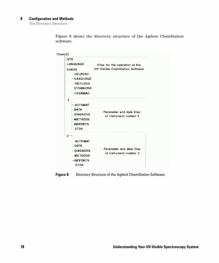
Figure 8 shows the directory structure of the Agilent ChemStation software.
Figure 8 Directory Structure of the Agilent ChemStation Software
78 Understanding Your UV-Visible Spectroscopy System
Configuration and Methods 8The Directory Structure
File Formats
All standard files associated with the Agilent ChemStation, both software and data, are in binary format, and therefore cannot be accessed (neither viewed nor edited) using standard text editing programs. This ensures compatibility with the guidelines of good laboratory practice (GLP).
When report to file is selected, the report is saved in ASCII format with the extension .TXT; report graphics are saved as Windows metafiles (binary format) with the extension .WMF.
Understanding Your UV-Visible Spectroscopy System 79
8 Configuration and MethodsThe Directory Structure
80 Understanding Your UV-Visible Spectroscopy System

Agilent ChemStation for UV-Visible SpectroscopyUnderstanding Your UV-Visible Spectroscopy System
9Verification
Configuration of Verification 82
Verification Tests 83
Spectrophotometer Selftests 92
Flow Test 93
81Agilent Technologies
9 VerificationConfiguration of Verification
Configuration of Verification
The information about the spectrophotometer and the filters used for the verification that you enter into the Instrument Verification Parameter dialog box is transferred into the Configuration of Verification table and can be stored in the configuration file (see “System Configuration” on page 68) by selecting the Save Configuration check box in the Close dialog box when you exit from the Agilent ChemStation software. There is no necessity to edit the configuration parameters thereafter unless you change one of the verification filters.
The other information in the Configuration of Verification table is transferred into the table automatically. The values are dependent on the spectrophotometer that is connected; to conform to the requirements of good laboratory practice (GLP), these values cannot be edited.
82 Understanding Your UV-Visible Spectroscopy System

Verification 9Verification Tests
Verification Tests
Wavelength Accuracy
An absorbance spectrum of an appropriate wavelength calibration standard is measured using 0.5 second integration time. This spectrum is converted into transmittance and the wavelength of specified peak minima are determined with the help of a spline function. The standards, reference wavelengths and specification used for the wavelength accuracy test are shown in Table 9.
NOTE The instrument should be allowed to warm up for a minimum of 45 minutes before running a verification.
Understanding Your UV-Visible Spectroscopy System 83
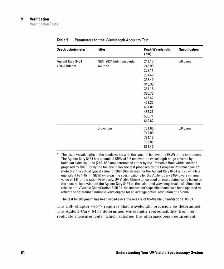
9 VerificationVerification Tests
Table 9 Parameters for the Wavelength Accuracy Test
Spectrophotometer Filter Peak Wavelength (nm)
Specification
Agilent Cary 8454190–1100 nm
NIST 2034 holmium oxide solution
241.13 249.98 278.11 287.40 333.49 345.38 361.18 385.70 416.42 451.33 467.86 485.26 536.71 640.62*
* The exact wavelengths of the bands varies with the spectral bandwidth (SBW) of the instrument. The Agilent Cary 8454 has a nominal SBW of 1.5 nm over the wavelength range covered by holmium oxide solution (240–650 nm) determined either by the “Effective Bandwidth” method proposed by NIST1 or by the toluene in hexane test proposed by the European Pharmacopoeia2 (note that the actual typical value for 269/266 nm ratio for the Agilent Cary 8454 is 1.75 which is equivalent to 1.45 nm SBW, whereas the specifications for the Agilent Cary 8454 give a minimum value of 1.6 for the ratio). Previously, UV-Visible ChemStation used an interpolated value based on the spectral bandwidth of the Agilent Cary 8454 as the calibrated wavelength values3. Since the release of UV-Visible ChemStation B.05.01, the instrument’s specifications have been updated to reflect the determined intrinsic wavelengths for an average optical resolution of 1.5 nm4.
The test for Didymium has been added since the release of UV-Visible ChemStation B.05.03.
The USP chapter <857> requires that wavelength precision be determined. The Agilent Cary 8454 determines wavelength reproducibility from ten replicate measurements, which satisfies the pharmacopeia requirement.
0.5 nm
Didymium 731.60740.00794.10799.00864.40
0.5 nm
84 Understanding Your UV-Visible Spectroscopy System
Verification 9Verification Tests
References:
1 NBS Special Publication 260- 66, Didymium Glass Filters for Calibrating the Wavelength Scale of Spectrophotometers, Venable W.H., Eckerle, K.L., October, 1979, p.70.
2 Pharmeuropa, Guide for the Technical Content of Monographs, Council of Europe, pp. 14- 15, 1993.
3 Agilent Application Note 5988- 9647EN, Wavelength accuracy and wavelength reproducibility of the Agilent Cary 8454 using holmium oxide solution, Klink, Thomas, June, 2003.
4 J Phys. Chem. Ref. Data. 34- 1, Intrinsic Wavelength Standard Absorption Bands in Holmium Oxide Solution for UV/visible Molecular Absorption Spectrophotometry, Travis et al, 2005, Table 1.
The calculation includes an additional acceptance tolerance of 0.1 nm for the NIST reference material and 0.2 nm for a holmium oxide solution because of the uncertainty of determining the true wavelength position of the peak. Upper and lower limits for the position of the measured peak are calculated from the used wavelength, the peak detection uncertainty and the specification:
(33)
and
(34)
The detected peak must lie within these two limits:
(35)
upper used specification uncertainty+ +=
lower used specification uncertainty+ +=
lower measured upper
Understanding Your UV-Visible Spectroscopy System 85
9 VerificationVerification Tests
Photometric Accuracy
By default, the NIST SRM 930 E 10% transmittance, neutral density glass standard is used for the photometric accuracy test.
Since the release of UV- Visible ChemStation B.05.03, the software allows for the measurement of up to three NIST- traceable neutral density glass standards to enable measurement of photometric accuracy at two or more absorbance levels. This is in compliance with the requirements of USP chapter <857> Ultraviolet-Visible Spectroscopy.
A spectrum is measured using the photometric accuracy filter with an integration time of 0.5 seconds at 440.0 nm, 465.0 nm, 546.1 nm, 590.0 nm and 635.0 nm.
(36)
where
Tnom is the nominal transmittance of the photometric accuracy filter
Ncalib is the age of the filter in months
Taging is the aging tolerance of the filter in transmittance
(37)
where
Taging is the aging tolerance of the filter in transmittance
e is the Euler constant
Substituting Equation 37 into Equation 36 gives Equation 38:
(38)
Taging
Ncalib
12------------- Tnom 1% =
Aaging e logTaging
Tnom--------------=
Aaging 0.00036191 Ncalib=
86 Understanding Your UV-Visible Spectroscopy System
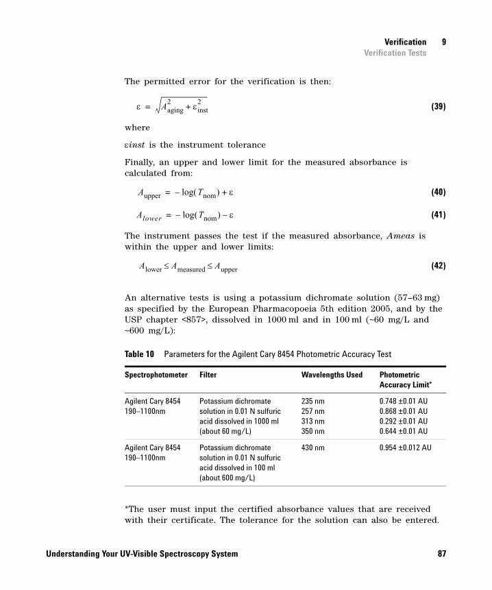
Verification 9Verification Tests
The permitted error for the verification is then:
(39)
where
inst is the instrument tolerance
Finally, an upper and lower limit for the measured absorbance is calculated from:
(40)
(41)
The instrument passes the test if the measured absorbance, Ameas is within the upper and lower limits:
(42)
An alternative tests is using a potassium dichromate solution (57–63 mg) as specified by the European Pharmacopoeia 5th edition 2005, and by the USP chapter <857>, dissolved in 1000 ml and in 100 ml (~60 mg/L and ~600 mg/L):
*The user must input the certified absorbance values that are received with their certificate. The tolerance for the solution can also be entered.
Table 10 Parameters for the Agilent Cary 8454 Photometric Accuracy Test
Spectrophotometer Filter Wavelengths Used Photometric Accuracy Limit*
Agilent Cary 8454190–1100nm
Potassium dichromate solution in 0.01 N sulfuric acid dissolved in 1000 ml(about 60 mg/L)
235 nm257 nm313 nm350 nm
0.748 ±0.01 AU0.868 ±0.01 AU0.292 ±0.01 AU0.644 ±0.01 AU
Agilent Cary 8454190–1100nm
Potassium dichromate solution in 0.01 N sulfuric acid dissolved in 100 ml(about 600 mg/L)
430 nm 0.954 ±0.012 AU
Aaging2 inst
2+=
Aupper log Tnom – +=
Alower log Tnom – –=
Alower Ameasured Aupper
Understanding Your UV-Visible Spectroscopy System 87
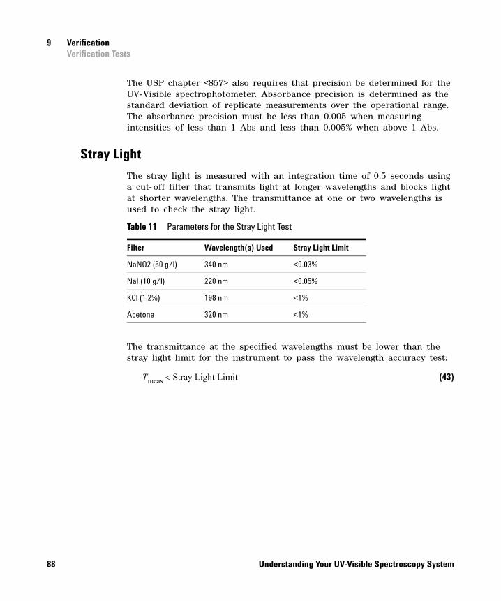
9 VerificationVerification Tests
The USP chapter <857> also requires that precision be determined for the UV-Visible spectrophotometer. Absorbance precision is determined as the standard deviation of replicate measurements over the operational range. The absorbance precision must be less than 0.005 when measuring intensities of less than 1 Abs and less than 0.005% when above 1 Abs.
Stray Light
The stray light is measured with an integration time of 0.5 seconds using a cut- off filter that transmits light at longer wavelengths and blocks light at shorter wavelengths. The transmittance at one or two wavelengths is used to check the stray light.
The transmittance at the specified wavelengths must be lower than the stray light limit for the instrument to pass the wavelength accuracy test:
(43)
Table 11 Parameters for the Stray Light Test
Filter Wavelength(s) Used Stray Light Limit
NaNO2 (50 g/l) 340 nm <0.03%
NaI (10 g/l) 220 nm <0.05%
KCl (1.2%) 198 nm <1%
Acetone 320 nm <1%
Tmeas Stray Light Limit
88 Understanding Your UV-Visible Spectroscopy System
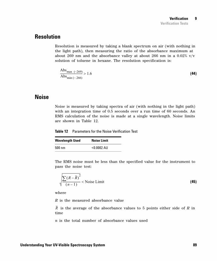
Verification 9Verification Tests
Resolution
Resolution is measured by taking a blank spectrum on air (with nothing in the light path), then measuring the ratio of the absorbance maximum at about 269 nm and the absorbance valley at about 266 nm in a 0.02% v/v solution of toluene in hexane. The resolution specification is:
(44)
Noise
Noise is measured by taking spectra of air (with nothing in the light path) with an integration time of 0.5 seconds over a run time of 60 seconds. An RMS calculation of the noise is made at a single wavelength. Noise limits are shown in Table 12.
The RMS noise must be less than the specified value for the instrument to pass the noise test:
(45)
where
R is the measured absorbance value
is the average of the absorbance values to 5 points either side of R in time
n is the total number of absorbance values used
Absmax (~269)
Absmin (~ 266)--------------------------------- 1.6
Table 12 Parameters for the Noise Verification Test
Wavelength Used Noise Limit
500 nm <0.0002 AU
R R– 2
n 1–
--------------------------- Noise Limit
R
Understanding Your UV-Visible Spectroscopy System 89
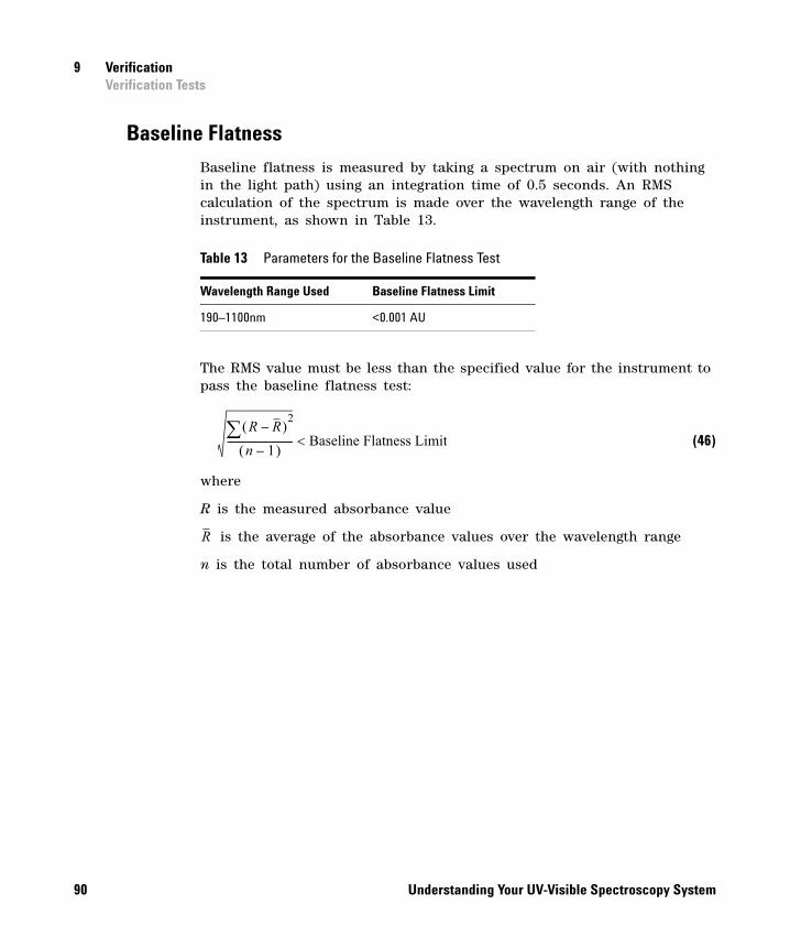
9 VerificationVerification Tests
Baseline Flatness
Baseline flatness is measured by taking a spectrum on air (with nothing in the light path) using an integration time of 0.5 seconds. An RMS calculation of the spectrum is made over the wavelength range of the instrument, as shown in Table 13.
The RMS value must be less than the specified value for the instrument to pass the baseline flatness test:
(46)
where
R is the measured absorbance value
is the average of the absorbance values over the wavelength range
n is the total number of absorbance values used
Table 13 Parameters for the Baseline Flatness Test
Wavelength Range Used Baseline Flatness Limit
190–1100nm <0.001 AU
R R– 2
n 1–
--------------------------- Baseline Flatness Limit
R
90 Understanding Your UV-Visible Spectroscopy System
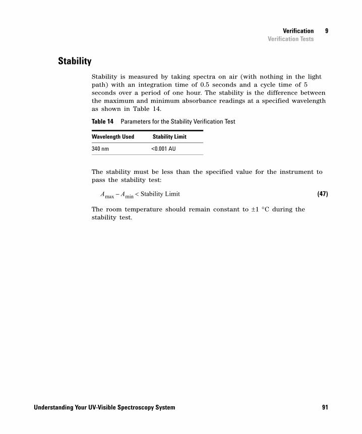
Verification 9Verification Tests
Stability
Stability is measured by taking spectra on air (with nothing in the light path) with an integration time of 0.5 seconds and a cycle time of 5 seconds over a period of one hour. The stability is the difference between the maximum and minimum absorbance readings at a specified wavelength as shown in Table 14.
The stability must be less than the specified value for the instrument to pass the stability test:
(47)
The room temperature should remain constant to 1 C during the stability test.
Table 14 Parameters for the Stability Verification Test
Wavelength Used Stability Limit
340 nm <0.001 AU
Amax Amin Stability Limit–
Understanding Your UV-Visible Spectroscopy System 91
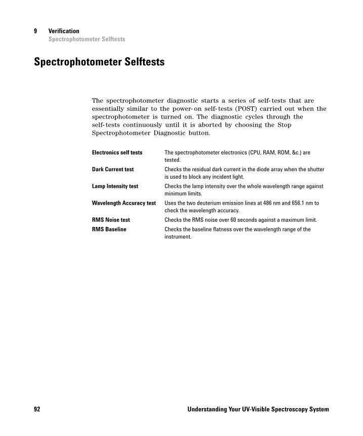
9 VerificationSpectrophotometer Selftests
Spectrophotometer Selftests
The spectrophotometer diagnostic starts a series of self- tests that are essentially similar to the power- on self- tests (POST) carried out when the spectrophotometer is turned on. The diagnostic cycles through the self- tests continuously until it is aborted by choosing the Stop Spectrophotometer Diagnostic button.
Electronics self tests The spectrophotometer electronics (CPU, RAM, ROM, &c.) are tested.
Dark Current test Checks the residual dark current in the diode array when the shutter is used to block any incident light.
Lamp Intensity test Checks the lamp intensity over the whole wavelength range against minimum limits.
Wavelength Accuracy test Uses the two deuterium emission lines at 486 nm and 656.1 nm to check the wavelength accuracy.
RMS Noise test Checks the RMS noise over 60 seconds against a maximum limit.
RMS Baseline Checks the baseline flatness over the wavelength range of the instrument.
92 Understanding Your UV-Visible Spectroscopy System
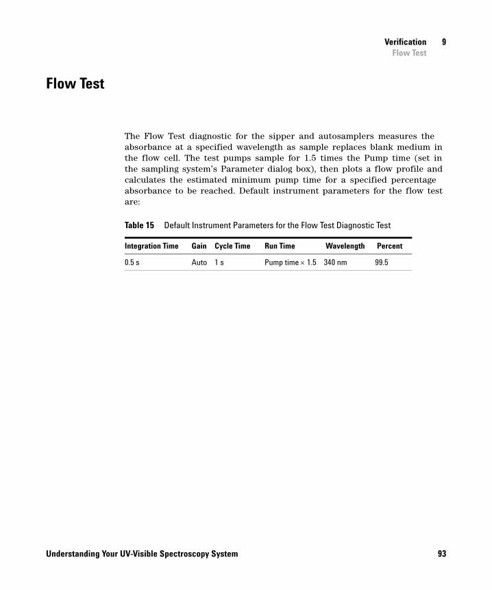
Verification 9Flow Test
Flow Test
The Flow Test diagnostic for the sipper and autosamplers measures the absorbance at a specified wavelength as sample replaces blank medium in the flow cell. The test pumps sample for 1.5 times the Pump time (set in the sampling system’s Parameter dialog box), then plots a flow profile and calculates the estimated minimum pump time for a specified percentage absorbance to be reached. Default instrument parameters for the flow test are:
Table 15 Default Instrument Parameters for the Flow Test Diagnostic Test
Integration Time Gain Cycle Time Run Time Wavelength Percent
0.5 s Auto 1 s Pump time 1.5 340 nm 99.5
Understanding Your UV-Visible Spectroscopy System 93
9 VerificationFlow Test
At the end of the run, the averages of the first two and last two measurements are calculated; the difference between the two averages gives the 100% difference in absorbance:
and
where
A is absorbance
n is the number of data points
The absolute absorbance value for the user- specified Percent objective is calculated by Equation 47:
(48)
where
Percent is the user- specified Percent objective
The flow profile is scanned to find the time, TE , at which the measured absorbance exceeds the absolute absorbance for the user- specified Percent objective, Auser%. This is the Estimated Minimum Pump Time.
A0%
A1 A2+
2------------------=
A100%
An 1– An+
2--------------------------=
Auser%
A100% A0%– Percent100
---------------------------------------------------------- A0%+=
94 Understanding Your UV-Visible Spectroscopy System
Index
Aabsorbance, 23, 34, 58
spectrum, 12accuracy
wavelength, 92acquisition
parameters, 71range, 53
add, 64analog-to-digital converter, 11analyte, 23, 41
name, 55analytes table, 23annotation limit, 52automation
method report, 51, 56parameters, 72results report, 51, 56table, 51, 56, 77
autosampler, 93autosave, 72
Bbackground correction, 35, 54baseline flatness, 90, 92Beer-Lambert law, 41binary functions, 64blank
measurement sequence, 56spectrum, 20, 69
Ccalibration, 16, 41, 42
coefficient, 17, 42coefficient k, 41curve, 42, 55curve fits, 45curve types, 42data, 15diagnostics, 21results, 48, 55standards, 44wavelength, 14
ChemStation.ini, 68ChemStation.ini file, 68, 75coefficient
calibration, 17, 42correlation, 49matrix, 61
color configuration, 68colors, 68comment, 23communication, 68
pathways, 68configuration, 20, 68
color, 68editor, 68file, 70, 82hardware, 68register, 70software, 68spectrophotometer, 69system, 20, 68temperature controller, 68
configuration of verification, 82table, 70
control samples, 56correlation coefficient, 49
current method, 17, 51, 53, 69, 72
Ddark current, 13
correction, 11test, 92
datablock, 21, 23, 24flow, 15raw, 10structure, 23type, 23, 54
data analysis, 73parameters, 20, 54, 72
data file, 77name, 55, 71
date, 23, 55, 72default, 68default path, 68derivative, 27, 34, 60
order, 60parameters, 60
dilution factor, 40, 56directory structure, 76, 78
Eeditor
configuration, 68electronics self tests, 92equation, 54
evaluation, 40name, 54parameters, 71
error%error, 48
error messages, 70
Understanding Your UV-Visible Spectroscopy System 95
Index
evaluation, 15, 17, 21equation, 40results, 51
Ffile
ChemStation.ini, 68configuration, 70, 82format, 79method, 72, 77
filter, 11filter length, 27, 60firmware, 10, 14, 23
revision number, 69firmware revision, 69flow
profile, 93test, 93
formula, 54function result, 21, 42
Ggraphical user interface files, 76graphics windows, 70
Hhardware configuration, 68header block, 23, 24
Iidentification number, 69indents, 52instrument
identification number, 23name, 53parameters, 20, 53, 71, 72type, 69
integration time, 12, 23, 53, 58intensity
lamp, 92spectrum, 11, 12
intercept, 42
invalid data, 14
Llamp
condition, 69intensity, 92
least squares fit, 60least squares method, 45
Mmacro files
system, 76user-generated, 76
margins, 52math result, 20mathematical operators, 28maxima, 27measurement sequence table, 56method, 69, 70, 71
description, 20, 71file, 72, 77file name, 53, 55, 56information, 53, 55, 72parameters, 72report, 51, 53
minima, 27molar extinction coefficient, 41
Nnoise, 89, 92
Oobject, 21
header, 21offset, 42on-line help files, 76operating software, 76, 77operator name, 23, 53, 55, 56optical system
UV-Visible spectrophotometer, 11
Pparameter files, 77parameters
acquisition, 71instrument, 20, 53, 71, 72method, 72printer setup, 52quantification, 71report, 70, 72report configuration, 52sampling system, 20, 71, 72spectral processing, 71spectrophotometer, 20, 53, 72stirrer, 71temperature controller, 72used wavelength, 71
password, 75path, 68
name, 55path length, 23, 40, 41peaks, 27, 54photometric accuracy, 86polynomial degree, 27, 60printer setup parameters, 52printing report, 74product number, 72pump time
estimated minimum, 93in flow test, 93
Qquadratic, 42quantification, 21, 41, 50
parameters, 71quantification task, 41
Rratio/equation task, 28raw data, 10, 20reference spectrum, 12register, 20
configuration, 70
96 Understanding Your UV-Visible Spectroscopy System
Index
reportconfiguration parameters, 52files, 77method, 51, 53orientation, 52parameters, 70, 72results, 51, 55
residual, 48resolution, 23, 89
wavelength, 64, 65results
calibration, 48, 55evaluation, 51report, 51, 55
RMS noise, 89
Ssample
measurement, 73name, 23, 70spectra, 20, 77temperature, 71
sample-related dynamics, 15sampling interval, 69sampling system, 70
parameters, 20, 71, 72Savitsky-Golay, 60scalar add, 63scalar divide, 63scalar multiply, 58, 63scalar subtract, 63self-tests, 92
electronic, 92serial number, 69shutter, 11single reference wavelength, 35sipper, 93software
configuration, 68revision number, 72
solvent, 23spectral data, 20spectral display limits, 54
spectral processing parameters, 71spectrophotometer
configuration, 69parameters, 20, 53, 72status, 69
spectrum/peaks task, 27stability, 91standard deviation, 23, 53, 58
of calibration, 48of coefficient, 49
standard spectra, 20, 77standards, 41, 44
minimum number, 44statistical errors, 45step, 62stirrer parameters, 71stored method, 72stray light, 11, 88
correction, 12subtract, 65subtract average over range, 37subtraction, 36system
configuration, 20, 68macro files, 76messages, 70
Ttable, 21
format, 70temperature, 23, 71temperature controller
configuration, 68parameters, 72
temporary registers, 21text file, 51three-point drop-line, 37time, 23, 55, 69, 72transmittance, 34, 59
Uunitary functions, 58
unknown sample, quantification, 50use wavelengths, 35used wavelength parameters, 71user interface display parameters, 71user-generated macro files, 76UV-Visible spectrophotometer
optical system, 11
Vvalleys, 27, 54variance, 12, 23, 58verification test results, 77view, 24volume, 28, 40
Wwavelength, 23
accuracy, 92calibration, 14range, 27, 64, 65resolution, 64, 65
weight, 28, 40window, 24
Understanding Your UV-Visible Spectroscopy System 97
Index
98 Understanding Your UV-Visible Spectroscopy System


Agilent Technologies 2000, 2003-2008, 2011, 2013, 2014, 2016
09/16
*G1115-90020**G1115-90020*G1115-90020
www.agilent.com
Agilent Technologies
In This Book
This manual describes the data processing operations of the Agilent Cary 8454 UV-Visible spectrophotometer and the Agilent ChemStation for UV-Visible spectroscopy. It describes the processes and transformations that the spectrophotometric data undergo between the time that they are acquired in the spectrophotometer and their output on the Agilent ChemStation display or printer. The manual is designed to enable you to follow good laboratory practice (GLP) guidelines; using the information in the manual, you will be able to understand the data processing calculations from beginning to end and perform the data evaluation manually.