agilent 85270 electromagnetic design...

emdsgs.book Tuesday, September 19, 2006 4:04 PM

Agilent 85270 Electromagnetic Design System

Getting Started

Agilent Technologies

EMDS Getting Started

Notices© Agilent Technologies, Inc. 2006

No part of this manual may be reproduced in any form or by any means (including elec-tronic storage and retrieval or translation into a foreign language) without prior agree-ment and written consent from Agilent Technologies, Inc. as governed by United States and international copyright laws.

Manual Part NumberOnline-only document

EditionOctober 2006

Printed in USA

Agilent Technologies, Inc.3501 Stevens Creek Blvd. Santa Clara, CA 95052 USA

Warranty

The material contained in this docu-ment is provided “as is,” and is sub-ject to being changed, without notice, in future editions. Further, to the max-imum extent permitted by applicable law, Agilent disclaims all warranties, either express or implied, with regard to this manual and any information contained herein, including but not limited to the implied warranties of merchantability and fitness for a par-ticular purpose. Agilent shall not be liable for errors or for incidental or consequential damages in connec-tion with the furnishing, use, or per-formance of this document or of any information contained herein. Should Agilent and the user have a separate written agreement with warranty terms covering the material in this document that conflict with these terms, the warranty terms in the sep-arate agreement shall control.

Technology Licenses The hardware and/or software described in this document are furnished under a license and may be used or copied only in accor-dance with the terms of such license.

Restricted Rights LegendU.S. Government Restricted Rights. Soft-ware and technical data rights granted to the federal government include only those rights customarily provided to end user cus-tomers. Agilent provides this customary commercial license in Software and techni-cal data pursuant to FAR 12.211 (Technical Data) and 12.212 (Computer Software) and, for the Department of Defense, DFARS 252.227-7015 (Technical Data - Commercial Items) and DFARS 227.7202-3 (Rights in Commercial Computer Software or Com-puter Software Documentation).

Safety Notices

CAUTION

A CAUTION notice denotes a haz-ard. It calls attention to an operat-ing procedure, practice, or the like that, if not correctly performed or adhered to, could result in damage to the product or loss of important data. Do not proceed beyond a CAUTION notice until the indicated conditions are fully understood and met.

WARNING

A WARNING notice denotes a hazard. It calls attention to an operating procedure, practice, or the like that, if not correctly per-formed or adhered to, could result in personal injury or death. Do not proceed beyond a WARNING notice until the indicated condi-tions are fully understood and met.

Microsoft ® is a U.S. registered trademark of Microsoft Corporation.

Windows ® and Microsoft Windows ® are U.S. registered trademarks of Microsoft Corporation.

Adobe ® and Acrobat ® are trademarks of Adobe Systems Incorporated.

Autodesk ® and AutoCAD ® are trademaks of Autodesk, Incorporated.

Software RevisionThis guide is valid for A.01.xx revisions of the Agilent 85270 Electromagnetic Design System software, where xx refers to minor revisions of the software that do not affect the technical accuracy of this guide.



Contents

1 System Overview 7

Overview 8

What is Electromagnetic Design System? 9

Quick and Accurate Modeling and Simulation 10No Numerical Electromagnetics Expertise Necessary 11Software Features 11

Modeling and Analysis Steps 13

Modeling the Structure 13Analyzing Electromagnetic Behavior 14

2 Drawing Geometric Models 17

Modeling Considerations 18

Making Efficient Models 19Getting Ready to Draw 20Program Basics 21

Drawing Examples 22

Drawing a Coax Tee-Junction 23

Setting Up the Project 25Drawing the Z-Axis Coax 27Drawing the Y-Axis Coax 33Uniting the Cylinders to Create the Tee-Junction 36Undo Command 38Parent and Child Objects 39Subtracting the Inner Cylinder Tee from the Outer Cylinder

Tee 39Slicing the Coax Tee-Junction 41

EMDS Getting Started 3

Contents


Saving the Coax Tee-Junction 42

Drawing a Microstrip Low-Pass Filter 45

Setting Up the Project 46Drawing the Dielectric 48Drawing the Air Box 50Defining a Reference Plane for the Microstrip 52Drawing the Microstrip 54Saving the Microstrip Low-Pass Filter 57

Drawing a Horn Antenna 58

Setting Up the Project 59Drawing the Base of the Horn 61Pan, Zoom, and Viewing Toolbar 63Drawing the Funnel Bottom 2D Rectangle 63Drawing the Horn Aperture 64Connecting 2D Objects to Create the Funnel 65Uniting the Horn Base with the Funnel 66Drawing the 3D Air Box Around the Horn Antenna 67Slicing the Structure Along Two Planes of Symmetry 68Editing and Deleting Drawing Objects 71

Drawing a Helix 72

3 Assigning Materials 75

Types of Materials 76

Metal 76Dielectric 76Semiconductor 76Resistor 77Solving Structures and Accounting for Lossy Materials 77

Coax Tee-Junction Materials 78

Microstrip Low-Pass Filter Materials 81

Horn Antenna Materials 84

4 EMDS Getting Started

Contents


4 Assigning Boundaries 85

Assigning Boundaries—Coax Tee-Junction 86

Defining Ports 89Defining Boundaries 91Defining Port Calibration and Impedance Lines 94

Assigning Boundaries—Microstrip Low-Pass Filter 99

Defining Boundaries 101Defining Port Calibration and Impedance Lines 102

Assigning Boundaries—Horn Antenna 104

Defining the Port 105Defining the Radiation Boundary 106Defining a Conductor Boundary 107Defining the Symmetry Plane Boundaries 107Defining the Aperture Boundary 108Defining an Impedance and Calibration Line 110

Entering a Voltage Source 113

5 Solving 117

Solve Setup 119

Solve Run 120

Batch Solving of Projects 120

Solve Job Control 121

Convergence Plots 121

Setting Up the Coax Tee-Junction 122

Solving the Coax Tee-Junction 125

Setting Up the Microstrip Low-Pass Filter 127

Solving the Microstrip Low-Pass Filter 131

Setting Up the Horn Antenna 132


Contents


Solving the Horn Antenna 135

6 Post Processing 137

Creating a Shaded Plot: Coax Tee-Junction 138

Rotating, Scaling, and Panning the Plot 141

Creating S-Matrix Plots: Microstrip Low-Pass Filter 143

Graph and Legend Properties 146

Viewing Far-Field Data: Horn Antenna 147

Creating a Far-Field Plot 147Creating a Polar Plot 148Viewing Antenna Parameters 150


Agilent 85270 Electromagnetic Design SystemGetting Started


1System Overview

Overview 8

What is Electromagnetic Design System? 9

Modeling and Analysis Steps 13

This manual is your guide to Electromagnetic Design System (EMDS). Designed for microwave engineers who have some experience with modeling passive structures, but are new to EMDS, it provides an introduction to and overview of the software, along with step- by- step examples for drawing, viewing, solving, and analyzing simple structures.

Examples demonstrate many important software features. Solved example files accompany the software and this manual and provide you with immediate, instructive sample geometries and results. Refer to these example files as you use this manual.

This manual is designed as the primary source of information for the first month or so of use of EMDS. For a complete list of software features, menus, options, and commands, refer to the Electromagnetic Design System User's Guide.

Before using this manual, be sure that EMDS is installed and configured for your hardware. Refer to the Electromagnetic Design System Windows Installation documentation for specific instructions.

7Agilent Technologies

1 System Overview


Overview

This chapter provides an introduction to Electromagnetic Design System. The chapter gives a brief product description and an overview of the basic steps for drawing, defining, solving, and analyzing modeling problems.

Figure 1 shows an example five- port waveguide structure and some resulting field patterns on selected planes that cut through the structure.

Figure 1 A Five-Port Waveguide Structure and its Electromagnetic Field Pattern


System Overview 1


What is Electromagnetic Design System?

EMDS is a software package for electromagnetic modeling of passive, three- dimensional structures. It computes:

• Scattering parameter (S- parameter) response for multiple modes

• Electric field distributions, including far- field antenna radiation patterns.

• Impedance and propagation constants for multiple modes

Use the EMDS drawing interface (based on the industry- standard AutoCAD drawing tool) to draw the geometry of any structure you are interested in modeling, or read in a 3D geometry that was created in Advanced Design System (ADS).

First, identify the ports, materials, and boundaries of the structure. Next, specify the frequencies and the desired accuracy. Then, solve for the electromagnetic fields. From this solution data, the post processor can derive:

• S- , Y- , and Z- parameter matrices, and re- normalized and de- embedded S- matrices

• Impedances and complex propagation constants at each port, for an unlimited number of modes

• Shaded and animated field plots

• Magnitude and phase plots displaying multiple traces for comparison with data from multiple simulations

• Vector and contour plots.

• Far- field plots—2D and 3D polar formats

• Quantity- versus- distance graphs of the field solutions

• Smith Chart plots

• Data tables


1 System Overview


Quick and Accurate Modeling and Simulation

The traditional, manual process for solid modeling and analysis consists of two- dimensional paper drafting, submitting the design to a model shop for prototyping, building the structure, testing it, and measuring its properties. This is typically called the “cut- and- try” process.

With EMDS, you can replace cut- and- try prototyping with computer modeling and analysis. The software makes it possible to draw and revise a model, or to construct a model from a library of commonly used parts. After creating the geometric model, you can view it from any angle and along any axis, in three dimensions.

Next, identify the materials of which the structure is made, and the structure’s ports and other boundary conditions.

Then specify the frequency or sweep of frequencies at which to solve for the electromagnetic behavior of the structure. You can specify such things as:

• The number of modes

• Voltage/Current input sources

• Convergence criteria, either for the entire S- parameter matrix or for specific S- parameters for each port and mode of interest

• The type of solve: single adaptive frequency, frequency sweep, or fast frequency sweep

A number of post- processing capabilities enable you to determine and observe the electromagnetic properties of the structure as field plots on the computer screen.

Saved scattering parameter data can be read by a number of circuit simulators, including other Agilent EEsof EDA circuit and systems design software.


System Overview 1


No Numerical Electromagnetics Expertise Necessary

If your knowledge of electromagnetics is limited, don’t worry. The EMDS modeling process consists of a short and logical set of steps for setting up and solving your problem. You don’t need numerical electromagnetics expertise to get accurate and reliable results, because the system does the calculations for you, to the degree of accuracy you specify.

Software Features

Electromagnetic Design System includes the following features:

• Uses Maxwell's equations to solve for electric and magnetic fields, and includes dispersion

• Runs on Windows platforms

• Uses the AutoCAD industry- standard interface to handle unrestricted geometries that can contain an unlimited number of dielectrics and ports

• Contains a solid model parts library that combines pre- drawn parameterized shapes such as filters, bends, striplines, and capacitors, to enter complex structures quickly and simply; parts are parameterized, so you can edit their dimensions to customize them for your own designs.

• Calculates scattering parameters for multi- port structures, to user- defined accuracy at each port and for each mode, if desired

• Calculates loss values when materials are characterized as lossy

• Contains a fast sweep mode for a fast preview of electromagnetic response


1 System Overview


• Contains a job control interface, enabling you to set up simulations to run after- hours, either locally or with remote simulation, to optimize computer resource usage; job control also makes it easy to check convergence progress

• Provides shaded and animated visual field patterns, field plots, graphs, and tables

• Allows for dynamic rotation of shaded plots to gain the best viewing angle

• Models radiating structures and calculates radiation patterns and related antenna parameters at all angles for detailed antenna performance analysis


System Overview 1


Modeling and Analysis Steps

This section gives the steps for creating a geometric model and analyzing its electromagnetic behavior.

Modeling the Structure

Modeling the structure includes entering its geometry and defining its materials, ports, and surfaces.

Drawing the Geometric Model

First, draw the structure using the industry- standard, AutoCAD- based, drawing interface.

An unlimited number of undo steps enable you to back out of any drawing process, one step at a time.

This final geometric drawing can be shaded and displayed from any angle and in a variety of colors to help you visualize the structure.

If your structure contains commonly used parts, you can draw it quickly by choosing your objects from the standard parts library that comes with the software.

Selecting Materials

You can select the materials the structure is made of as you draw objects, or you can choose objects and define materials after the structure is complete. Choose from the supplied materials database, or enter your own materials, along with the appropriate parameters, such as permeability and permittivity, as well as conductivity if the material is a lossy metal, magnetic loss tangent and electric loss tangent if the material is a lossy dielectric, and resistivity if the material is a resistor.


1 System Overview


Defining Ports and Boundaries

Next, define the boundaries for the structure, and define and calibrate the ports.

Boundary types include perfect magnetic or electric conductor, magnetic or electric symmetry boundary, a conductive boundary, a resistive boundary, a ground plane, or a radiation boundary.

Ports can be waveguides, coaxial connectors, or virtually any type of transmission line. You can draw impedance, calibration, and polarization lines for each port and mode of interest. The system solves and calculates the field solution for each port, and provides useful data such as port impedance.

Analyzing Electromagnetic Behavior

Once the model is complete, run the simulator and the post processor to analyze the structure.

Solving for the S-Parameters

The simulator uses a mathematical technique known as finite element analysis to determine the field quantities and S- parameters. From the EMDS Solve > Setup menu pick, you can choose to solve for the generalized scattering parameters at one adaptive frequency, for a frequency sweep, or for a fast frequency sweep.

S- parameters can be normalized with respect to the port impedances. If you plan to include the S- parameters in a circuit simulation, you can re- normalize them to 50 ohms with a simple menu command.

Perform an adaptive refinement of the finite- element mesh to achieve results that fall within a user- specified accuracy.

For quick, 2D analysis of the ports of the structure, specify a ports- only solution.


System Overview 1


For a quick preview of a structure’s frequency response, use the fast frequency sweep. This fast sweep saves time by solving the problem at a single frequency and then using a rational function approximation for the frequency bandwidth of interest.

Analyzing the Results

After the simulation is complete and the S- parameters are calculated for the model, use the post- processing features to display the numerical results and to display field distributions graphically.

Port shading, surface shading, and plane shading provide a visual representation of wave propagation and electromagnetic characteristics on the computer screen.

Animated shaded field plots shift the phase at which the plot is shown, simulating the fields as they propagate through the structure in real time. You can rotate these shaded plots to gain various perspectives and an optimum viewing angle for the structure.

You can display and print far- field, vector, and contour plots and graphs, and Smith Chart graphs, as well as tables of S- parameter data.


1 System Overview





2Drawing Geometric Models

Modeling Considerations 18

Drawing Examples 22

Drawing a Coax Tee-Junction 23

Drawing a Microstrip Low-Pass Filter 45

Drawing a Horn Antenna 58

Drawing a Helix 72

This chapter gives examples that emphasize the drawing features of Electromagnetic Design System (EMDS). The examples use many of the commands that are available for drawing, editing, and viewing a wide variety of geometries.


2 Drawing Geometric Models


Modeling Considerations

Although the drawing tools in EMDS are flexible and make it possible to draw nearly any geometry, modeling problems must be realistic and within the scope of the software's analytical capabilities.

Note these general rules:

• When modeling enclosed structures, make the enclosure a realistic size.

The enclosure surrounding the geometric model of a structure automatically accounts for packaging effects. When drawing microstrip structures, a good general rule is to allow a distance of at least five substrate thicknesses from the strip to the outside of the enclosure.

• When modeling open- region problems, designate the enclosure as a radiation boundary.

Open- region problems, such as antenna and radiation problems, are solved by drawing an enclosure around the antenna and designating the enclosure as a radiation boundary. The absorbing boundary can be placed close to the structure, and it can be arbitrarily shaped.

• Unless a circuit source is specified, structures must have at least one port.

In the absence of a port, a circuit source can be applied to a structure. If a circuit source is not used, then at least one port is needed to make a measurement.

• Diodes, transistors, or other active devices cannot be simulated.

Static bias fields cannot be applied in the simulator.

Conductivity can be infinite for metals, or metals can have a finite conductivity. The dielectric constant can be real or complex. A complex dielectric constant accounts for the loss tangent.

• Structures should not contain moving parts.


Drawing Geometric Models 2


Moving parts cannot be simulated directly. However, by defining different geometries by moving or rotating parts of the structure, the electromagnetic effects of the moving parts can be inferred.

• Structures should be kept electrically small.

Because the simulator calculates the electromagnetic fields at every point in space as defined by the tetrahedral mesh, keep structures to a reasonable size. Trial and error will help you determine when a structure has become too complicated for a particular computer platform. A good general rule is to simulate structures that are only a few wavelengths long.

To simulate electrically large structures, try to split the geometry into subsections along the axis of wave motion. The individual subsections can then be simulated and the resulting S- matrices can be combined.

Making Efficient Models

Because the algorithms that are used to solve Maxwell's equations are time- and computer- memory- intensive, keep these additional considerations in mind when drawing geometric models:

• Make the drawing of the structure as simple as possible.

Rounded corners, for example, are much more complex and time- consuming to simulate than are square corners. If an area of the structure has rounded corners but the area is not electrically important, draw them as square corners to save time and computer memory. Via holes, for example, often can be drawn and modeled as flat, 2D strips.

• Take advantage of symmetry.

If you know that the structure has electric or magnetic symmetry, take advantage of it by defining the symmetry plane or planes and solving just a symmetrical part of the structure. Using symmetry reduces problem size and




decreases solve time. Be sure, however, that you do understand the symmetry characteristics of a problem before you use symmetry.

Getting Ready to Draw

When getting ready to draw a geometric model of a structure:

• Have a mental picture of the structure. You might want to sketch the structure on paper and include the dimensions as a reference.

• Think of the structure in its component pieces. You may even want to sketch an exploded view.

• If the structure is complex, list the objects that make up the complete structure.

• Remember that you typically model the interior space of structures where the electromagnetic waves travel, and not the walls of the structure.

Also be aware that often you can simplify the physical representation of the structure because some of the complexity of the actual part is not significant to the electromagnetic simulation. For example, highly faceted corners or arcs might not be needed to approximate an actual curved surface—a large segment angle might suffice. As another example, you can model conductors as 2D strips rather than as 3D objects, thus eliminating the need for a 3D mesh for the conductor.

NOTE There is often more than one way to draw, or to enter coordinates for, any geometric model. The steps for drawing the examples in this chapter are simply one set of drawing options. Experiment with the drawing commands to develop efficient methods for creating your own geometric models.




Program Basics

You may want to read through Chapter 1 of the Electromagnetic Design System User’s Guide before beginning the first exercise.




Drawing Examples

Use the step- by- step guidelines in this chapter to draw the following example geometric models:

• Coax tee- junction

• Microstrip low- pass filter

• Horn antenna

• Helix

The commands that are used in this chapter provide you with a foundation from which you can work to draw and create your own geometric models.

For a complete listing and a description of every drawing command, refer to the Electromagnetic Design System User's Guide.




Drawing a Coax Tee-Junction

The coaxial tee- junction is simple to draw, and yet it illustrates a number of useful drawing commands, such as unite, subtract, and slice.

When thinking of the drawing problem, remember that you are modeling air space that represents the dielectric, and not the coaxial conductor itself. In other words, the area of interest is the area between the perimeter of the inner cylinder and the perimeter of the outer cylinder, as in Figure 2.

This is why the inner cylinders are essentially “drilled out” with the subtract command, and the area of interest is specified as air. The inner cylinders that are subtracted become the inner boundary of the area of interest, and are filled with a perfect electric conductor (metal) as a default.




The following general steps outline the coax tee- junction drawing process:

• Draw the inner and outer 3D cylinders for the coax that lies on the Z axis.

• Draw the inner and outer 3D cylinders for the coax that lies on the Y axis.

• Unite the Z- and Y- axis outer cylinders, then unite the Z- and Y- axis inner cylinders.

• Subtract the inner, united object from the outer, united object.

• Slice the coax tee- junction in half along the Y,Z plane.

Detailed instructions for drawing the coax tee- junction follow.

Figure 2 Modeling Area of Interest: Coax Tee-Junction




Setting Up the Project

To get ready to draw the coax tee- junction, create and name the project, and set the project preferences, such as drawing grid, units, and snap options.

Creating and Naming the Project

To name the new project:

1 Start the software. The EMDS Agilent EMDS Startup dialog box appears. Click the Open Project Manager button to open the Project Management dialog box.

2 In the Project Management dialog box, use the Directory Browser to specify the location where your new project will be saved. You can change this if you want, but make sure you have write permissions to the directory you choose.

3 In the Project Management dialog box, click New. The New Project dialog box is displayed.

4 Verify that the correct Directory path is displayed for the New Project and enter the name coaxtee in the Project name field. This is the project folder where the new project, coaxtee, will be saved. All files associated with this project will be stored in the coaxtee directory.

5 Press Return or click OK. The Project Preferences dialog box is displayed.

NOTE Although we recommend that you work through this drawing example yourself, if you do not want to draw the coax tee now, refer to the pre-drawn example in the waveguide examples project folder. The example project name is coaxt.




Setting the Project Preferences

The Project Preferences dialog box is displayed as a default whenever you begin a new project. It is a reminder to set your units and grid settings appropriately for your project.

1 For this example, use the settings that are shown in Figure 3.

2 Click OK. The main screen is displayed.

Note that the name of the new project is displayed in the main screen title bar.

Figure 3 Coax Tee-Junction Project Preferences




Drawing the Z-Axis Coax

To draw the Z- axis coax, draw the inner and outer cylinders in the XY plane. This is the default reference plane, so you should not have to define it first. The grid is always displayed across the current reference plane.

Drawing the Outer Cylinder

To draw the outer cylinder:

1 Choose Model > Draw. The draw screen is displayed and the menu bar changes.

2 Choose 3D Objects > Cylinder. Information is displayed in the text area at the bottom of the window, instructing you to choose the center of the cylinder.

3 Move the pointer near the X,Y origin and click the left mouse button to define the center of the cylinder.

Don’t worry about getting the cursor exactly on the origin. You’ll be able to set all the coordinates after you click an outer point for the cylinder and the resulting template dialog box is displayed.

An alternate way to enter 2D and 3D objects is to type their coordinates in the text box that appears in the lower window of the EMDS screen.

This is how you will enter the low- pass filter in the next drawing example.

4 As you move the pointer away from the center point, a circle appears on the screen. It shrinks and grows as you move the mouse.

5 Click the left mouse button to define an outer edge for the cylinder.

Again, don’t worry about the size of the circle. You’ll be able to adjust it with specific coordinates in the template dialog box.

6 Refer to the dialog box in Figure 4 and use the displayed origin, dimensions, and other data for your cylinder.




Cylinder Template Explanation

Note the fields in the template dialog box:

• Segment Angle—This is used to determine the number of sides the circle has. The bigger the angle, the coarser and less refined the circle. The smaller the angle, the more sides there are to the circle and the more refined and smooth the circle is. Because the coax tee- junction is a simple structure that will not require a lot of computer resources to solve, you can use 15- degree segment angle here.

Figure 4 Cylinder Template for the Outer Z-Axis Cylinder

NOTE For many structures, 30-degree angles or even coarser resolutions are sufficient for accurate S-parameter analysis.




• World or Local Coordinates—The world coordinate system is a fixed Cartesian coordinate system that uses three axes—X, Y, and Z—to specify locations in two- or three- dimensional space. The local coordinate system is determined by the reference plane defined and selected under the Define menu. To use a local coordinate system, specify the location and the orientation of an object in the UV plane.

• Object Name—Although this field is filled with a name as a default, it is useful to type in a more descriptive name. In Figure 4, the object name is xycylout, because the name indicates that this is the outer part of the coax that lies in the XY plane.

• Object Color—You can select any color to change the color of the cylinder as it is displayed.

• Materials—It is easy to define materials for objects as you go, by selecting a material and checking the box for Use in Simulation. Since this object does not yet represent the complete coax, don’t worry about using it in the simulation or defining materials for it.

7 When the dialog box is filled out to your satisfaction, click OK.

The cylinder is created along the Z axis, as in Figure 5.




Editing Parameterized Objects

In EMDS, object parameters (dimensions, location in space, segment angles, and so on) are saved with the objects you draw. You can refer to and edit these object parameters to make changes to a structure. Object parameterization can be very handy for fine- tuning structures to achieve a desired response or for doing “what- if” analyses.

The parameters for most 2D and 3D objects are saved with the project unless you delete the objects. You can keep objects with a structure just for editing purposes. The object can be set to be invisible, or set to be left out of the simulation, or both, with the commands Objects > Visible, and Objects > Simulation.

For the coax tee- junction example, the cylinders that are used to create the complete coax are saved with the structure as parameterized objects.

Figure 5 Z-Axis Outer Cylinder




To modify objects:

1 From the draw screen, choose Objects > Object Parameters. The Parametric Object Information dialog box is displayed.

2 Click the object you want to edit. The template for the object is displayed.

Objects that are created from other objects, such as uniting 3D objects or connecting 2D objects, do not have parameters stored for the resulting objects—only for the objects that were used to make the united or connected object. In addition, arbitrarily- shaped polygons which are created using the polyline command are not parameterized.

3 Edit any of the parameters you want then click OK when you are finished. The drawing on your screen reflects your changes.

Drawing the Inner Cylinder

To draw the inner cylinder, follow the same steps as you did to draw the outer cylinder, using the different dimensions for the cylinder, as shown in Figure 6. Use the name xycylin to describe the inner cylinder that lies in the XY plane.




Your resulting inner and outer cylinders should look like the ones in Figure 7.

Figure 6 Cylinder Template for the Inner, Z-Axis Cylinder




Drawing the Y-Axis Coax

To draw the Y- axis coax, draw the outer and inner cylinders in the ZX plane. Because this is not the default plane, you will need to set the drawing area to display this plane first.

Setting the ZX Plane

1 From the draw screen, choose Define > Plane Set.

The plane list is displayed.

2 Choose ZX plane, and click OK. The grid is displayed in the ZX plane, indicating the plane where you will be drawing.

Drawing the Outer and Inner Cylinders in the ZX Plane

To draw the outer and inner cylinders in the ZX plane, follow the same instructions as for drawing the Z- axis coax.

Choose 3D Objects > Cylinder, and specify a center and an outer edge for the cylinder. Then use the dimensions in Figure 8.

Figure 7 Z-Axis Outer and Inner Cylinders.




For the inner cylinder, choose 3D Objects > Cylinder, and specify a center and an outer edge for the inner cylinder. Then use the dimensions in Figure 9.

Figure 8 Cylinder Template for the Outer Y-Axis Cylinder




To help you view the structure more clearly, choose Window > Shade > Hidden.

The resulting drawing should look like the one in Figure 10.

Figure 9 Cylinder Template for the Inner Y-Axis Cylinder




Uniting the Cylinders to Create the Tee-Junction

To create the junction between the Z- axis and the Y- axis pieces of coax, use the 3D Objects > Unite command.

1 Choose 3D Objects > Unite. The Object Unite dialog box is displayed.

2 From the list of 3D Objects, hold down the Ctrl key, and click xycylout and xzcylout.

3 In the Object Name field, type a more descriptive name, such as coaxout.

4 Click Apply. The united, outer cylinders are displayed in the project window, as in Figure 11.

Figure 10 All of the Cylinders that Make up the Coax Tee-Junction.




5 This time, hold down the Ctrl key and select xycylin and xzcylin, and name the resulting object coaxin.

6 Click OK. The inner cylinders are united to form the inner part of the coax tee.

7 Choose Window > Shade > 3D Wireframe to view the inner cylinder shown in Figure 12.

Figure 11 United Outer Cylinders




Undo Command

If you make a mistake using the unite command, choose Edit > Undo to cancel the last command. You can repeatedly choose undo up to the first command performed after choosing Model > Draw. Once you return to the main screen you cannot use undo to cancel completed drawing commands.

Figure 12 United Inner and Outer Cylinders




Parent and Child Objects

When you view the lists of 2D and 3D objects during an edit command, you may notice that some objects are indented in the list. An indented object is a child object; the parent object is the next object above it that is not indented at the same level. Parent objects are created from the child objects

To see the relationships between the original cylinders, and united objects created from them:

1 Choose Objects > Object Parameters. The Parametric Object Information dialog box is displayed.

2 Look at the list of 3D objects carefully. The parent objects are coaxin and coaxout. Their child objects are listed below each of their names, slightly indented. The child objects of coaxin are xycylin and xzcylin. The child objects of coaxout are xycylout and xzcylout.

Subtracting the Inner Cylinder Tee from the Outer Cylinder Tee

As discussed at the beginning of this chapter, and shown in Figure 2 on page 24, the modeling area of interest—where the electromagnetic fields propagate—is the area between the inner and outer cylinders.

The Subtract command is designed to remove overlap between objects, so there are several extra steps required to subtract the inner cylinders from the outer cylinders. Another way of looking at this is to imagine that you are drilling out the inner cylinder to allow for the inner perfect conducting boundary.

NOTE Not all drawing commands result in parent-child relationships, although there is generally an association formed. For example, when you copy an object neither object is indented under the other, but until you unlink them, any changes made to the original will result in changes to the copy.




To subtract the inner cylinder:

1 Choose 3D Objects > Subtract. The Object Subtract dialog box is displayed.

2 From the Core 3D Objects list, click coaxout.

3 From the Subtracted 3d Objects list, click coaxin.

4 In the Object Name field, type coaxtee.

5 Leave the field Use in Simulation checked, because you will be simulating the resulting object.

If you are in doubt whether to check the box Use in Simulation, don’t worry. You can always edit it with the command Objects > Simulation. Also, you will get another chance to edit this when you save your project.

6 In the Material field, click air.

If you are in doubt about what material to assign to an object, don’t worry. You can assign materials later, from the main screen, when you set ports and boundary conditions for the structure.

7 Click OK.

In the subtraction process, a copy of coaxin is actually subtracted from coaxout, thus removing any overlap that might have occurred between the adjacent objects. So coaxin actually remains part of the model, and must be either deleted or set so that it is not included in the simulation.

8 Choose Edit > Delete. The Object Delete dialog box appears.

9 Select coaxin and enable Delete object and its base objects.

10 Click OK. The system pauses while the inner cylinder tee is subtracted from the outer cylinder tee.

Alternatively, you could have chosen Objects > Simulation, selected coaxin, and clicked Do not use selected objects in simulation. Further, you could make coaxin invisible through Objects > Visible.

Although the objects do not look any different on the screen, the inner tee- junction cylinder has been subtracted from the outer tee- junction cylinder. In other words, the inner metal conductor of the coax tee- junction has been “drilled out.”




Slicing the Coax Tee-Junction

When electric or magnetic symmetry exists for a structure, you can slice the drawing of the structure, define the slice boundary as a electric symmetry or a magnetic symmetry boundary, and then solve for the part of the structure that remains after the slice. Or, you can simply draw one- half, one- quarter, or even a smaller part of a structure and accurately model the complete structure.

Solving just part of a structure saves time, disk space, and memory space. Be aware, however, that just because a structure has geometric symmetry does not mean that it has electric or magnetic symmetry.

Because the coax tee- junction has perfect magnetic symmetry when it is cut in half along the YZ plane, it is convenient to slice the geometric model of the coax tee- junction in half along this plane. Later, when you solve the problem, it will solve faster, and the solution will take up less disk space.

To slice the coax tee- junction:

1 Choose Edit > Slice. The Object Slice dialog box displayed.

2 From the 3D Objects list, click coaxtee.

3 From the Plane list, click YZ plane.

4 Click OK.

The coax tee- junction is sliced in half along the YZ plane, displaying the half that extends into the positive X direction, as in Figure 13.

NOTE Choose Window > Shade > Hidden to see the object more clearly.




Saving the Coax Tee-Junction

Choose File > Save from the draw screen at any time to save your drawing work. It is a good idea to save your work periodically, especially when you are drawing complicated structures.

Choose Objects > Simulation. The Object Simulation dialog box is displayed, as shown in Figure 14.

Figure 13 Sliced Coax Tee-Junction

NOTE You may want change the orientation of the drawing using the Window > Viewing Direction command.




The list of objects shows which objects are visible (a V is displayed to the left of the object name), and which objects are selected to use in the simulation (an S is displayed to the left of the object name).

All of the objects you used to create other objects are saved with the project unless you explicitly delete them, even though they do not show up in this dialog box, and are not visible. If you need them again to create more objects, you can edit their parameters, and the drawing will be updated automatically.

For this example, the sliced coaxtee shows up in the dialog box, because it is the only parent object. You will define materials, ports, and boundaries only for this object, and only it will be used in your simulation.

Figure 14 Object Simulation Dialog Box




Because you can see the coaxtee on the screen, it is marked as being visible (V). Make sure that the coaxtee is also marked as being used in the simulation (S), and click OK to dismiss the dialog box.

Choose File > Return to Main to go back to the main screen. You have finished drawing the coax tee- junction.




Drawing a Microstrip Low-Pass Filter

This section gives step- by- step instructions for drawing a microstrip low- pass filter. Refer to Figure 15 for its dimensions and port locations.

For this example, draw only one- half of this structure, because the microstrip low- pass filter has magnetic symmetry.

Use this general procedure to draw the microstrip low- pass filter:

• Set up the project.

• Draw and position one- half of the 3D rectangle that represents the substrate.

Figure 15 Dimensions of the Complete Microstrip Low-Pass Filter




• Draw and position one- half of the 3D rectangle that represents the air enclosure.

• Draw one- half of the 2D microstrip.

Each of these steps is described in this section.


To get ready to draw the microstrip low- pass filter, create and name the project, and set the project preferences.



1 Use the Directory Browser to change to the directory where you want to store your project.

2 Open the Project Manager by choosing Project > Project. The Project Management dialog box is displayed.


4 Verify that the correct Directory path is displayed for the New Project and enter the name lpfilter in the Project name field. This is the project folder where the new project, lpfilter, will be saved. All files associated with this project will be stored in the lpfilter directory.


NOTE Although we recommend that you work through this drawing example yourself, if you do not want to draw the microstrip low-pass filter now, refer to the pre-drawn example in the planar examples project folder. The example project name for this exercise is ms_lpf.





The Project Preferences dialog box is displayed as a default whenever you begin a new project. It is a reminder to set the units and grid settings appropriately for your project.

1 For this example, use the settings shown in Figure 16.

2 Click OK. The main screen is displayed.

The name of the new project is displayed in the main screen’s title bar.

Figure 16 Project Preferences—Microstrip Low-Pass Filter




Drawing the Dielectric

To draw the dielectric for the microstrip low- pass filter, refer to Figure 15 on page 45 for the dimensions of the dielectric, and follow these steps:

1 From the main screen, choose Model > Draw. The draw screen is displayed.

2 Choose 3D Objects > Box. The prompt displayed in the text area at the bottom of the window is instructing you to choose an initial corner of the box.

3 Move the pointer near the X,Y origin and click the left mouse button to define a corner of the box.

Don’t worry about getting the cursor exactly on the origin. You will be able to set all the coordinates after you click to define the opposite corner of the box, and the resulting Box Template is displayed.

Move the pointer to an opposite corner for the box. Notice that a rectangle is drawn on the screen, and that it shrinks and grows as you move the mouse.

4 Click the left button to define the opposite corner of the box.

Don’t worry about the size of the box. You will be adjusting it with the Box Template that is displayed.

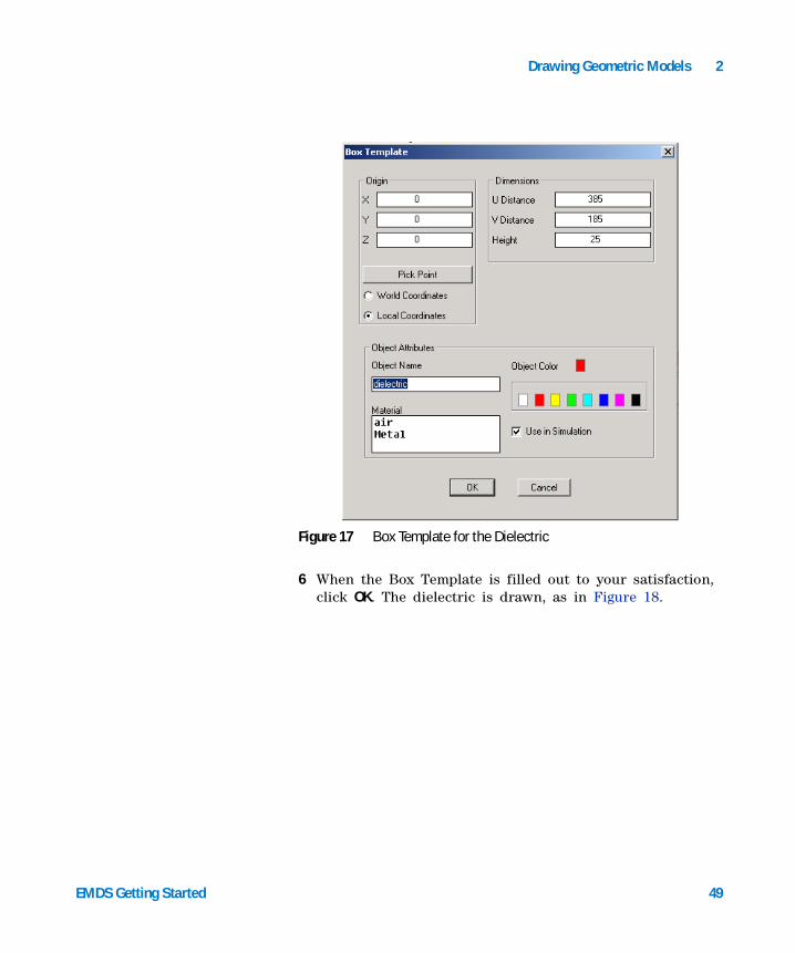
5 Refer to the dialog box in Figure 17, and use the displayed data for your box. This object is named dielectric.




6 When the Box Template is filled out to your satisfaction, click OK. The dielectric is drawn, as in Figure 18.

Figure 17 Box Template for the Dielectric




Drawing the Air Box

To draw the air box that encloses the microstrip low- pass filter, refer to Figure 15 on page 45 for the dimensions of the air box, and follow these steps:

1 From the draw screen, choose 3D Objects > Box. The prompt displayed in the text area at the bottom of the window is instructing you to choose an initial corner of the box.

2 Move the pointer near the X,Y origin and click the left mouse button to define a corner of the box.

Because you left Snap to Object Points checked in the Project Preferences dialog box, when you click near the origin your initial point will snap to the origin of the dielectric. This will be useful for drawing the air box, because the coordinates for the box will be correct in the resulting dialog box.

3 Move the pointer to an opposite corner for the box. A rectangle is drawn on the screen, and it snaps to the opposite corner of the dielectric.

Figure 18 One-Half of the Dielectric




4 Click the left button to define the opposite corner of the box. The Box Template is displayed.

5 Refer to the dialog box in Figure 19, and use the displayed dimensions and other data for your box. This object is named airbox.

6 When the Box Template is filled out to your satisfaction, click OK. The air box is drawn, as in Figure 20.

Figure 19 Box Template for the Air Box




Both the air box and the dielectric are parameterized objects you can edit at any time with the Objects > Object Parameters command.

Defining a Reference Plane for the Microstrip

Before you draw the microstrip, define the plane on which to place it. You want the 2D object to rest on top of the dielectric. Therefore, define a reference plane that is 25 mils up from the XY plane, where the top of the dielectric lies.

1 Choose Define > Plane Define. The Define Plane dialog box is displayed.

2 Click Pick Plane.

The dialog box goes away so you can see the draw screen. In the text area at the bottom of the screen you are prompted for the origin.

3 Place the pointer on the U,V origin of the top of the dielectric and click the left mouse button. Watch the pointer closely to make sure it is snapping to the object

Figure 20 One-Half of the Dielectric and Air Box




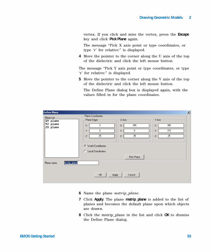
vertex. If you click and miss the vertex, press the Escape key and click Pick Plane again.

The message “Pick X axis point or type coordinates, or type ‘r’ for relative:” is displayed.

4 Move the pointer to the corner along the U axis of the top of the dielectric and click the left mouse button.

The message “Pick Y axis point or type coordinates, or type ‘r’ for relative:” is displayed.

5 Move the pointer to the corner along the V axis of the top of the dielectric and click the left mouse button.

The Define Plane dialog box is displayed again, with the values filled in for the plane coordinates.

6 Name the plane mstrip_plane.

7 Click Apply. The plane mstrip_plane is added to the list of planes and becomes the default plane upon which objects are drawn.

8 Click the mstrip_plane in the list and click OK to dismiss the Define Plane dialog.




Drawing the Microstrip

To draw the microstrip, use the Polyline command and use the text area at the bottom of the screen to enter numbers corresponding to the relative offsets for each point you want to enter.

To draw the microstrip:

1 From the draw screen, choose 2D Objects > Polyline.

To draw the polyline enter consecutive points between which lines are drawn. When you use the keyboard to do this, it is generally easiest to enter an absolute coordinate set for the first point in the U,V coordinate system. Then, use relative offsets so that each subsequent point you enter is referenced to the previous point you entered.

The prompt “Pick first point or type coordinates” is displayed in the text area of the screen.

2 Type the values 0, 185, and press Return.

The first point is placed on the edge of the dielectric, and the text area prompts you to pick or to enter another point, or press r for relative offset.

Note that you can cancel any point that you add by clicking the right mouse button. You can leave the polyline entry mode completely by pressing the Escape key.

3 Type r.

The text are displays the message “Pick next point or type relative offset, or type a for absolute.”

4 Type 0, -12.5, and press Return.

The first line of the microstrip is drawn on the screen.




5 Type the remaining points, pressing Return after each one:

70,0

0,-60

45,0

0,65

65,0

0,-125

25,0

0,125

65,0

0,-65

45,0

0,60

70,0

0,12.5

-385,0

With the entry of the last point the line segments close, forming a 2D object, and the 2D Object Completion dialog box is displayed (see Figure 21).

6 In the Object Name field, type microstrip. Then click OK.

Figure 21 2D Object Completion Dialog Box




The set of line segments should look like the ones in Figure 22.

Figure 22 Completed, One-Half of Microstrip Low-Pass Filter




Saving the Microstrip Low-Pass Filter

You have finished drawing the microstrip low- pass filter. When you return to the main screen, verify that the dielectric, air box, and microstrip are all marked visible and to be used in simulation.

1 Choose File > Save from the draw screen to save your drawing work. It is a good idea to save your work periodically, especially when you are drawing complicated structures.

2 Choose File > Return to Main to go back to the main screen.

3 Choose Objects > Simulation. The Object Simulation dialog box is displayed. The list of objects shows which objects are visible (a V is displayed to the left of the object name), and which objects are selected to use in the simulation (an S is displayed to the left of the object name).

4 For this example, the three sliced objects show up in the dialog box: the dielectric, the air box, and the microstrip.

Because you can see these objects on the screen, they are marked as visible (V). Make sure that they also are marked as being used in the simulation (S).

5 Click OK to return to the main screen.




Drawing a Horn Antenna

The horn is a simple antenna structure. To draw it, use another useful drawing command, the connect command, to create a 3D object from the two 2D objects that make up the top and bottom of the horn.

Refer to Figure 23 for a sketch of the horn antenna with its dimensions.

The following general steps outline the horn antenna drawing process:

• Draw the box that makes the 3D base of the horn.

• Draw a 2D rectangle on top of the base to represent the bottom of the horn funnel.

Figure 23 Dimensions of the Horn Antenna




• Draw a 2D rectangle to represent the aperture of the horn.

• Connect the two, 2D objects to create the 3D horn funnel.

• Unite the horn base with the horn funnel.

• Create a 3D air box around the horn antenna.

• Reduce the problem size by slicing the structure along two planes of symmetry.

Detailed instructions for drawing the horn antenna follow.


To get ready to draw the horn, create and name the project, and set the drawing grid and units.



1 Open the Project Manager by choosing Project > Project. The Project Management dialog box is displayed.

2 Using the Directory Browser in the Project Management dialog box, change to the directory where you want to store your project.


4 Verify that the correct Directory path is displayed for the New Project and enter the name horntutor in the Project name field. This is the project folder where the new

NOTE Although we recommend that you work through this drawing example yourself, if you do not want to draw the horn antenna now, refer to the pre-drawn example in the antenna examples project folder. The example project name for this exercise is horn.




project, horntutor, will be saved. All files associated with this project will be stored in the horntutor directory.



The Project Preferences dialog box is displayed as a default whenever you begin a new project. It is a reminder to set your units and grid settings appropriately for your project.

1 For this example, use the settings shown in Figure 24.

2 Then click OK. The main screen is displayed. The name of the new project is displayed in the main screen’s title bar.

Figure 24 Horn Antenna Project Preferences




Drawing the Base of the Horn

The base of the horn has a uniform cross- section that is rectangular and has the dimensions 0.4 inches wide by 0.9 inches long by 0.315 inches high. To draw it, create a 3D rectangle and set its dimensions with the template that is displayed.

Follow these steps:

1 From the main screen, choose Model > Draw. The draw screen is displayed, and the menu bar changes.

2 Choose 3D Objects > Box. A message is displayed in the text area of the screen, prompting you for an initial corner of the box.

You can either type in a set of comma- separated coordinates (for example, 0,0 for the origin) or click anywhere in the active drawing window.

3 Click anywhere in the active drawing window. Move the pointer, and click again to define the opposite corner of the box. It does not matter where you draw this box, because you will be able to adjust all of its dimensions with the Box Template. The Box Template is displayed.

4 Fill out the template as in Figure 25. Then click OK. The antenna base is drawn on the draw screen.




Figure 25 Box Template for the Horn Antenna




Pan, Zoom, and Viewing Toolbar

To adjust the magnification or change the viewing direction of the box on the screen for better visibility, use the icons that are displayed in the toobar (see Figure 26) to zoom in, zoom out, or zoom to a window size you specify.

Window zoom and viewing direction options are also available from the Window > Zoom and Window > Viewing Direction menus.

To pan the object, you can use the Window > Pan options.

For more information on the options described above, refer to the EMDS User’s Guide.

Drawing the Funnel Bottom 2D Rectangle

To create the “funnel,” or tapering part of the horn antenna, draw two rectangles, and then connect them to create the 3D funnel. Place the first rectangle directly on top of the 3D antenna base you just drew.

Figure 26 Example EMDS Toolbar

All

Window

Dynamic

In

Out

Zoom Commands

SW Isometric

SE Isometric

NE Isometric

NW Isometric

3D Orbit

Viewing Direction Commands




To do this, follow these steps:

1 Choose Window > Project Preferences. The Project Preferences dialog box is displayed.

2 Select Snap to Object Points, and then click OK.

3 Choose 2D Objects > Rectangle.

4 Move the pointer to one corner of the bottom of the antenna base, and click the left mouse button.

Snap to Object Points only finds vertices in the current reference plane.

5 Move the pointer to the opposite corner of the bottom of the antenna base, and click again. The Rectangle Template is displayed.

The length and width of the rectangle match those of the antenna base.

6 Enter .315 in the Z coordinate field so the rectangle is positioned on top of the horn base.

7 Name the rectangle funnel_base, and click OK. A 2D rectangle is drawn on top of the antenna base.

Drawing the Horn Aperture

Next, draw the 2D rectangle that represents the top of the funnel, or the aperture of the horn.

Follow these steps:

1 Choose 2D Objects > Rectangle.

2 Move the pointer somewhere above the box that already is displayed, and click to define a corner of the aperture.

3 Move the pointer to an opposite corner of the aperture, and click again. The Rectangle Template is displayed.

NOTE You may want to change the color of the funnel base in order to see it. Use Objects > Recolor and select the funnel_base in the 2D Objects list in the Object Recolor dialog box to change the color.




4 Fill out the template as in Figure 27. Then click OK. A 2D rectangle is drawn that represents the aperture of the horn.

Connecting 2D Objects to Create the Funnel

Now you can connect the 2D objects that make up the base and the top of the funnel to create the 3D, funnel- shaped object.

Figure 27 Rectangle Template for Horn Aperture




To connect the rectangles:

1 Choose 3D Objects > Connect. A message is displayed in the text area of the screen, prompting you to select a point on a 2D object.

2 Click one corner of the top 2D object to select it. Then click the corresponding corner of the bottom 2D object to select it as well. If you incorrectly select any point, click Edit > Undo and carefully select the point again. The Connect Template is displayed.

3 Name the object funnel, and click OK. The 3D funnel is displayed above the horn base.

Uniting the Horn Base with the Funnel

Although it is not strictly necessary, you will unite the two 3D objects—the horn base and the funnel—to create one 3D horn antenna structure. This makes the problem simpler by keeping the number of objects to a minimum.

To unite the base and the funnel:

1 Choose 3D Objects > Unite. The Object Unite dialog box is displayed.

2 In the list of 3D Objects, hold down the Shift key, and click both objects—base and funnel.

3 Name the new object horn. Then click OK. The completed horn antenna is displayed.

It does not look any different than it did before the union, yet the object named horn is the result of all the steps you have taken up to this point.

All of the 2D and 3D objects that you have used so far to create the horn are saved with the project and can be edited to change the size and shape of the horn if desired.




Drawing the 3D Air Box Around the Horn Antenna

To simulate the horn antenna, you need to enclose it in a bounded “box” of air.

To draw the air box:

1 Choose 3D Objects > Box.

2 Draw a rectangle in the drawing space. The Box Template is displayed.

3 Fill out the template as in Figure 28. Then click OK.

You’ve drawn the complete horn antenna structure, as in Figure 29.

4 Save your project with the File > Save command.

Figure 28 Box Template for the Air Box




Slicing the Structure Along Two Planes of Symmetry

To reduce problem size, it is a good idea to take advantage of symmetry by solving just a symmetrical part of the problem. This saves time and computer resources, solving the problem quicker and with smaller file sizes.

The horn antenna is a symmetrical structure that has planes of symmetry in two directions—along the YZ plane the problem has electric symmetry, and along the ZX plane the problem has magnetic symmetry. Therefore, you can slice this structure to one quarter of its full size and solve just a quarter of the problem.

Figure 29 Complete, Horn Antenna Drawing




To slice the horn antenna in two directions:

1 From the draw screen, choose Edit > Slice. The Object Slice dialog box is displayed.

2 Click all of the 3D objects to select them for slicing.

3 Select the YZ plane from the Plane List. Then click OK. The horn structure is sliced along the YZ plane, as in Figure 30.

2D objects cannot be sliced. That is why you still see the complete 2D objects used to create the funnel.

Because these objects will not be used in the simulation, it does not matter that they are visible. But, if you want to make the drawing look more attractive, you have two choices:

• Turn the visibility of the 2D objects off with the Edit > Visible command.

• Delete the 2D objects (since you will not need them again) with the Edit > Delete command.

Figure 30 Slice of Horn Antenna Along the YZ Plane




4 Choose Edit > Slice again. The Object Slice dialog box is displayed.

5 Select all of the 3D objects.

6 Select the ZX plane from the Plane List. Then click OK. The horn structure is sliced again, this time along the ZX plane, to leave only one- quarter of the structure, as in Figure 31.

Figure 31 One-Quarter of the Horn Antenna




Editing and Deleting Drawing Objects

As mentioned in the coax tee- junction drawing example, EMDS enables you to edit the dimensions of your drawings by editing the objects you used to create the drawing.

1 Click Objects > Object Parameters, and select the 2D or 3D object you wish to edit. If the object is editable, the template with the dimensions and coordinates of the object is displayed.

2 Modify the values in any of the fields that are displayed in the template.

3 Click OK and the results of the modification are displayed on the screen.

Objects that are created as a result of connecting or uniting other objects cannot be edited. When connecting two 2D objects, for example, you can edit the original, 2D objects, but you cannot directly edit the 3D object that is the result of using the Connect command.

It is a good idea to keep all of the 2D and 3D objects you used to create other objects until you are sure you will not need them again to edit your structure’s dimensions. When you are sure you do not need objects that you used to create the structure, explicitly delete them if you want, with the Edit > Delete command. If you do not delete them, they are saved with the project.




Drawing a Helix

The helix is a common structure in antenna design. This example shows how easy it is to draw one. To solve a typical helix antenna problem, you would place a uniform cross- section at the base of the helix for a port, and then enclose the entire structure to create a radiation boundary. For this example, however, you will simply draw the helix itself.

To draw a helix:

1 Return to the Project Manager to create a new project, and name it helix.

2 When the Project Preference dialog box is displayed, set the units to millimeters, and click OK.

Don’t worry about the other settings on the dialog box for this example.

3 Choose Model > Draw.

4 From the draw screen, choose Object Library > Helix.

5 Click somewhere near the origin of the UV plane for the center of the helix.

6 Move the mouse. A circle is drawn on the screen indicating the outer edge of the helix.

7 Click anywhere to define the outer edge of the helix. The Helix Template dialog box is displayed.

8 Give the helix the dimensions shown in Figure 32.




9 Click OK. The system pauses while it computes the helix.

10 Use Window > Zoom > Window to expand the size of the helix so that you can readily see it.

• Move the pointer to a spot near the helix, and click to define a corner of the zoom window.

• Move the pointer to draw a box around the helix, and click again to define the opposite corner of the box.

The resulting, zoomed helix drawing should look like the one in Figure 33.

Figure 32 Helix Template




11 To get an even better look at the resulting helix, try using the command Window > Shade > Hidden.

The resulting helix should look like the one in Figure 34.

Figure 33 Resulting, Finished Helix

Figure 34 Resulting, Finished Helix, with Hidden Lines Removed




3Assigning Materials

Types of Materials 76

Coax Tee-Junction Materials 78

Microstrip Low-Pass Filter Materials 81

Horn Antenna Materials 84

As mentioned in Chapter 2, “Drawing Geometric Models”, you can assign the materials your structures are made of as you draw the structure. The drawing templates, where you define the parameters for 2D or 3D objects, enable you to specify whether the object will be used in the simulation as well as the material of which the object is made. The materials listed in the drawing templates are the ones you have included in the material database. To define a material that is different than the ones in the database, use the main screen menu command Materials > Assignment.


3 Assigning Materials


Types of Materials

Use the Material Assignment dialog box to define the appropriate values for the following types of materials:

• Lossless or lossy metal

• Isotropic or anisotropic dielectric

• Semiconductor

• Resistor

Metal

An object defined as metal can be either a perfect electrical conductor or a lossy material. Lossy metals have a conductivity value associated with them so that the simulator can make an accurate surface impedance approximation.

Dielectric

An object defined as a dielectric can be either isotropic (uniform properties in all directions, such as with alumina) or anisotropic (permittivity, permeability, electric loss tangent, and magnetic loss tangents that vary with direction, such as with sapphire).

Use magnetic loss tangent to specify a lossy magnetic material. Use electric loss tangent to specify a lossy dielectric material.

Semiconductor

A semiconductor material, such as a silicon semiconductor, can be a 2D or a 3D object. You specify the properties of a semiconductor either in resistivity or in conductivity. Since


Assigning Materials 3


one of these values is always the inverse of the other, when you enter one value the other is automatically updated by the system.

You can also specify a permeability and a permittivity value for semiconductors.

Resistor

Resistors, although they are highly process- dependent, are typically modeled as 2D objects and specified in Ohms per square.

If you model a resistor as a 3D object, you will need to enter a resistivity value for it, in ohm- meters.

Solving Structures and Accounting for Lossy Materials

Any structure that can be solved using loss can also be solved without loss.

The advantages of solving problems with loss include:

• More accurate and realistic results are obtained for certain classes of structures; for example, stripline structures that contain a resistor.

• Lossy definitions allow you to simulate a load (a resistor), resistive loads, terminations, and structures containing imperfect conductors such as gold or copper. You cannot accurately simulate such structures without accounting for loss.

In this chapter we’ll define materials for the following examples:



• Horn antenna




Coax Tee-Junction Materials

Because the coax tee- junction is composed only of air, it would have been easy to define the material for it when drawing the structure in Chapter 2, “Drawing Geometric Models.”

To view the material assignment for the coax tee- junction example:

1 From the EMDS Project Management dialog box, open the project coaxtee if you completed the example, “Drawing a Coax Tee- Junction” on page 23, or open the pre- drawn coax tee- junction example by choosing the waveguide examples project folder and opening the project coaxt.

2 From the main screen, choose Materials > Assignment. The Material Definition dialog box is displayed.




3 Select the object coaxtee from the Object List.

4 In the Project Material List, click air.

5 Click Edit Material. The Dielectric Definition dialog box is displayed.




Air is defined as having a permittivity and a permeability value of 1. These are the appropriate values.

6 Click Cancel to exit the dialog box.

7 Click OK to exit the material definition.




Microstrip Low-Pass Filter Materials

The microstrip low- pass filter example consists of an air box, a substrate, and a microstrip filter. Each of these objects is defined as a material, and each has its own set of characteristics.

To assign materials for the microstrip low- pass filter:

1 From the Project Management dialog box, open the project lpfilter if you completed the example, “Drawing a Microstrip Low- Pass Filter” on page 45.

If you did not draw and save the microstrip low- pass filter as an exercise in Chapter 2, you can open and view the pre- drawn microstrip low- pass filter example by choosing the planar examples project folder and opening the project ms_lpf.


3 From the Object List, select the 3D object airbox. Then, in the Project Material List, select air.

4 From the Object List, select dielectric.

5 In the Material Name field, type alumina.

6 In the Material Type section, select Dielectric.

Because alumina has consistent material properties in all directions, it is an isotropic material. Therefore, you do not need to click the anisotropic check box.

7 Click New Material. The Dielectric Definition dialog box is displayed.

8 Use the typical values for alumina shown in Figure 35.




9 Click OK.

10 Select alumina to assign it to the dielectric.

11 From the Object List, select the 2D object microstrip. Then, in the Project Material List, select Metal.

12 Click Edit Material. The Metal Definition dialog box is displayed.

13 Deselect Perfect Conductor.

14 Fill in values for conductivity and permeability as in Figure 36. Then click OK.

Figure 35 Values for Defining Alumina as a Dielectric

Figure 36 Metal Definition Dialog Box with Values for the Metal Mi-crostrip




All of the materials for the microstrip low- pass filter are assigned.

15 Click OK to close the dialog box.

Later on, when you define ports and boundaries for this structure, you will define the two ports of the structure, and the electric symmetry boundary along the slice of the microstrip low- pass filter.




Horn Antenna Materials

In the horn antenna example, both the horn itself and the air box surrounding the horn are composed of air. You could have defined these objects as air as you drew the structure, or you can define them now, with Materials > Assignment.

To define materials for the horn antenna:

1 From the EMDS Project Management dialog box, open the project horntutor if you completed the example, “Drawing a Horn Antenna” on page 58. If you did not draw and save the horn antenna as an exercise in Chapter 2, you can open and view the pre- drawn horn antenna example by choosing the examples project folder and opening the project horn.


3 Fill out the dialog box by selecting each 3D object (horn and airbox), and selecting air as the material for each object.

4 Click OK.

In the next chapter, when you define ports and boundaries for this structure, you will define the radiation boundary for the horn and open the top of the horn to allow the structure to radiate into the air box.




4Assigning Boundaries

Assigning Boundaries—Coax Tee-Junction 86

Assigning Boundaries—Microstrip Low-Pass Filter 99

Assigning Boundaries—Horn Antenna 104

Entering a Voltage Source 113

Define boundaries for the surfaces of your structures, so the simulator can take into account the characteristics of the materials used by the structure. Define ports to let the simulator know where energy can enter and leave the structure. Before assigning boundaries:

• Specify at least one object in the structure for use in the simulation.

• Materials must be assigned to all objects that are to be used in the simulation.

In the exercises in this chapter, you will define boundaries for the following examples:



• Horn antenna

NOTE You can think of boundary assignments like paint; the last one you use is the one that the software “sees” and recognizes. So the order in which you place boundaries can be important. The exception to this rule is with ports. A boundary that is defined as a port always takes precedence over all other boundary conditions.


4 Assigning Boundaries


Assigning Boundaries—Coax Tee-Junction

The coax tee- junction consists of a coaxial transmission line with an inner and an outer metal boundary. Refer to Figure 37 to see the location of the various ports and boundaries for the sliced (one- half of the actual structure), coax tee- junction.

Figure 37 Boundary and Impedance/Calibration Line Locations—Coax Tee-Junction


Assigning Boundaries 4


The coax tee- junction has three ports. Because it has been split in half to take advantage of its magnetic symmetry, the coax tee- junction also has a symmetric magnetic boundary.

To define the boundaries for the coax tee- junction:

1 From the EMDS Project Management dialog box, open the project coaxtee if you completed the example, “Drawing a Coax Tee- Junction” on page 23, or open the pre- drawn coax tee- junction example by choosing the examples project folder and opening the project coaxt.

2 From the main screen for the coax tee- junction example, choose Boundaries > Add. The Define Port or Boundary Condition dialog box is displayed.

NOTE To facilitate applying ports and boundaries, if you are using the structure that you created in “Drawing a Coax Tee-Junction” on page 23, you may want to reorient the view using NE Isometric View under Window > Viewing Direction.




Defining Ports

The coax tee- junction has three ports. To define them:

1 From the Define Port or Boundary Condition dialog box, click Enter Number of Ports and Modes. The Define Number of Ports and Modes dialog box is displayed.

2 The default settings are two ports and one mode per port. Change the entry for Define the Number of Ports to 3.

3 Leave Define the Number of Modes set to 1.

For this example, you will solve for the dominant, or first- order mode only. You could enter any number of modes here to solve the problem for higher- order modes as well.

Even though you can solve for any number of modes per port, you should limit the number of modes to just those you truly need. The more modes you specify, the larger and more complex the resulting S- parameter matrix. Solving for many modes also adds to the overall solve time for your problem.

Figure 38 Number of Ports and Modes




4 To set the impedance multiplier, you must first click one of the ports in the Select a Port and Allocate its Modes list, and then type .5 in the Impedance Multiplier field. Do this for each port in the list.

The impedance multiplier is set to .5 because the coax tee- junction has a Symmetric H plane of symmetry, therefore, the unmodified values are two times those of the full structure. By setting the Impedance Multiplier field to .5, the system will accurately calculate the impedance of the full structure.

The settings are shown in Figure 38 above.


6 Make sure Port is checked as the type. From the list under Port #, click 1.

7 Click Add.

8 Select 3 Point Plane. The dialog box disappears, enabling you to see the structure and to select three points that define the plane where the port lies.

It is easiest to pick a port this way when Snap to Object Points is checked in the Window > Project Preferences dialog box, and when Snap to Grid Points is unchecked. It may also be helpful to zoom in on the port.

9 Place the pointer near a point on port 1 of the coax tee- junction and click it. Refer to Figure 37 on page 86 for the location of the ports. A small x is drawn on the vertex point to indicate it is selected.

10 Place the pointer near two more points on the port and click them. When three points on one plane have been selected, a confirmation dialog box is displayed, and the port is highlighted

.




11 When the port is selected correctly, click OK. The Define Port or Boundary Condition dialog box is re- displayed, and an asterisk (*) is displayed next to port 1, indicating it is defined.

12 Follow steps 6 through 11 to identify ports 2 and 3.

Defining Boundaries

The magnetic boundary along the YZ plane is the boundary you created when you sliced the coax tee- junction in half. Choose this plane and define it as a symmetric H plane that will be taken into account when the problem is solved.

To define the symmetric H boundary:

1 From the list of boundary types in the Define Port or Boundary Condition dialog box, click Symmetric H Plane.

A boundary name of Symmetric_H_Plane_4 is listed in the Boundary Name field. You can change this name if you want, but use the default for now.

2 Click Add at the bottom of the dialog box.

3 Click 3 Point Plane. The dialog box disappears, enabling you to see the structure and to select three points that define the plane where the boundary condition lies.

4 Place the pointer near a point on the symmetry plane of the coax tee- junction and click it. Refer to Figure 37 on page 86 for the location of the magnetic (H) symmetry plane. A small x is drawn on the vertex point to indicate it is selected.

5 Place the pointer near two more points on the plane and click them. When three points on one plane have been selected, a confirmation dialog box is displayed, and the plane is highlighted.

6 When the symmetry plane is selected correctly, click OK.

You have defined all the necessary boundaries for the coax tee- junction.




There are a number of other types of boundaries you can use for various types of structures. For details about each of these boundaries, refer to the Electromagnetic Design System User’s Guide.

7 Click Done to close the dialog box.

Displaying Boundaries

To verify you have defined the ports and boundaries correctly, you can display and view them with the command Boundaries > Display.

To display the boundaries for the coax tee- junction:

1 Choose Boundaries > Display. The Display Boundary Condition dialog box is displayed.

2 Choose a port or boundary, and select a separate color and design for each one.

You can also set the scale for the design to make it easier to see.




An outer boundary is listed, although you did not define an outer boundary in the previous section. The outer boundary is always assigned as a default, and you can display it here.

Click Clear or Clear All to clear the display of selected or of all boundaries.

3 Click Draw to display the boundaries you have chosen. You can draw and display these boundaries one at a time, or you can define all of the boundaries.

You can move the dialog box to the side by grabbing its title bar and dragging it out of the way so you can see your structure.

4 When you are satisfied with boundary display, click Done.

An example of displayed boundaries for each port and boundary of the coax tee- junction is shown in Figure 39.

Figure 39 Displayed Boundaries for the Coax Tee-Junction




Querying Boundaries

After displaying boundaries, you can query each boundary to see its name. To do this:

1 With the boundaries displayed on the screen, click Boundaries > Query. The message, Select the boundary hatch to query is displayed in the text area at the bottom of the screen.

2 Click any hatch line of any displayed boundary. The text area at the bottom of the screen displays the name of the boundary.

Defining Port Calibration and Impedance Lines

Because you can predict where the energy fields will be the greatest at the ports for the coax tee- junction, you can set impedance lines at the ports. These lines make it possible for the system to calculate the impedances at the ports when the problem is solved.

For the coax tee- junction, the energy fields for the first- order mode are greatest radially, from the center edge to the outside edge of each port.

The calibration line for the coax tee- junction sets the direction of the phase at each port. Then, when the problem is solved, the phase will align with the direction of the calibration line.

For this example, the calibration line and the impedance can be the same line, so you need to draw only one line per port. A polarization line is not required for this example.

Polarization lines force degenerate modes to align with the polarization line. Polarization lines typically are used with circular or square waveguide problems, where polarization of degenerate modes is possible.

Setting impedance, calibration, and polarization lines is optional. It is not required as a step before solving problems. It is a good idea, however, to define port calibration lines for




all problems to eliminate a 180- degree phase shift ambiguity in S- parameters. It is also a good idea to define impedance lines for all structures so power- voltage and voltage- current impedances are calculated.

Refer to Figure 37 on page 86 for the location of ports, impedance and calibration lines on the coax tee- junction example.

Solving and Displaying E Fields

To verify the correct location of your impedance lines, you can view the E- field at the ports. To do this:

1 Use the tool bar or the Window > Zoom command to zoom in on port 1.

2 From the main screen, choose Boundaries > Port Calibration. The Port Impedance / Calibration / Polarization Lines dialog box is displayed.

3 If it is not already selected, click Port # 1 and Mode # 1.

4 Set Frequency to 10 GHz, and set Scale to Full.

5 Click Solve and Display E Field. The message box, “computing the port solution” is displayed.

6 When the port solution is complete, move the Impedance/Calibration/Polarization Lines dialog box out of the way to see the display of the E- fields for port 1.

NOTE Impedance, calibration, and polarization lines only operate on individual ports. Be sure to define them for every port in the structure.




Because you set the scale of the arrows to Full, all of the arrows are the same size, and they simply indicate the direction of the E- field. If you set the scale to Linear, the length of the arrows will vary, so you can observe both direction and field strength.

A setting of Log gives a logarithmic scaling of the field strength and direction.

7 When you are through viewing the E- fields, click Done to close the dialog box. This will clear the arrows from the port.

Drawing the Impedance and Calibration Lines for the Ports

To draw the impedance and calibration line for port 1:

1 Make sure Snap to Object Points is selected in Window > Project Preferences.

2 Choose Boundaries > Port Calibration.




3 Make sure Port #1 and Mode #1 are highlighted, and in the Line Types area select Impedance and Calibration.

4 In the area labeled Start, click Pick Point. The dialog box disappears, allowing you to pick a point on port 1.

Refer to Figure 37 on page 86—the impedance and calibration line starts at the outer edge of the port and points inward, in other words, from the reference ground to the signal line.

5 Click a point on the outer edge of the port. The Port Impedance/Calibration/Polarization Lines dialog box is re- displayed.

Values are now filled in for the X, Y, and Z coordinates of the starting point.

6 In the area labeled End, click Pick Point. The dialog box disappears, allowing you to pick a point on port 1.

7 Click a point on the inner edge of the port. The Port Impedance/Calibration/Polarization Lines dialog box is re- displayed.

Values are now filled in for the X, Y, and Z coordinates of the end point, and the impedance/calibration line is drawn on the port, as in Figure 40.




8 Click Apply.

9 Click the next port number, and repeat steps 4 through 8 to draw impedance/calibration lines for ports 2 and 3. Be sure to click Apply after picking points for each one.

10 When lines have been defined for each port, click Done. Ports, port calibration and boundaries are defined for the coax tee- junction, and it is ready to solve.

11 Choose Project > Save to save your port calibration work.

Figure 40 Displayed Impedance/Calibration Line for Port 1

Impedance/Calibration Line




Assigning Boundaries—Microstrip Low-Pass Filter

The microstrip low- pass filter requires two ports: one for the signal to enter the structure and one for the signal to exit the structure. Refer to Figure 41 for the location of the ports and boundaries.

The outer surface of the model is defined by default as a perfect conductor. In addition, because impedance boundaries are specified by a conductivity value, an impedance boundary is defined for the microstrip.

You can also define an impedance line at each of the ports if you know where the tangential electric field lines will be the greatest, and you can calibrate the ports to prevent a

Figure 41 Ports, Boundaries, and Impedance/Calibration Lines for the Microstrip Low-Pass Filter

Symmetric H plane

Port 2

Port 1

Impedance/calibration line




random, 180- degree phase shift. In the microstrip low- pass filter, you know the field will be the greatest for the first- order mode from the center of the full microstrip to the bottom of the dielectric. The system then calculates the Zpv and Zvi impedances at each of the ports for the modes you request. Zpi is always computed unless the outer port boundary contains no conductors.

To define the ports for the microstrip low- pass filter:

1 From the EMDS Project Management dialog box, open the project lpfilter that you completed in “Drawing a Microstrip Low- Pass Filter” on page 45, or open the pre- drawn example by choosing the examples project folder and opening the project ms_lpf.

2 From the main screen, choose Boundaries > Add. The Define Port or Boundary Condition dialog box is displayed.

3 From the Define Port or Boundary Condition dialog box, click Enter Number of Ports and Modes. The Number of Ports and Modes dialog box is displayed.

The default settings are two ports and one mode per port. This is correct.

4 Click PORT 1 MODES 1 IMPEDANCE 1 to select it.

5 Because the microstrip low- pass filter has a magnetic symmetry boundary, enter a value of .5 in the Impedance Multiplier field.

6 Click PORT 2 MODES 1 IMPEDANCE 1 to select it.

7 Again, enter a value of .5 in the Impedance Multiplier field. Then click OK. The Number of Ports and Modes dialog box disappears.

8 Make sure Port is checked as the type. From the Port # list, click 1.

9 Click Add.

10 Select 3 Point Plane. The dialog box disappears, enabling you to see the structure and to select three points that define the plane where the port lies.




It is easiest to pick a port this way when Snap to Object Points is checked and Snap to Grid Points is unchecked in Window > Project Preferences.

11 Place the pointer on a point on port 1 of the microstrip low- pass filter and click it. Refer to Figure 41 on page 99 for the location of the ports. A small x is drawn on the vertex point to indicate that it is selected.

12 Place the pointer on two more points on the port and click them. When three points on one plane have been selected, a confirmation dialog box is displayed, and the port is highlighted.

13 When the port is selected correctly, click OK. The Define Port or Boundary Condition dialog box is re- displayed, and an asterisk (*) is displayed next to port 1, indicating that it is defined.

14 Follow steps 8 through 13 to define port 2. Refer to Figure 41 on page 99 for its location if necessary.

Defining Boundaries

The magnetic symmetry boundary shown in Figure 41 on page 99 is the boundary you created by only drawing one- half of the microstrip low- pass filter. Choose this plane and define it as a symmetric H plane that will be taken into account when the problem is solved.

To define the symmetric H boundary:

1 From the list of boundary types in the Define Port or Boundary Condition dialog box, click Symmetric H Plane. A boundary name of Symmetric_H_Plane_3 is listed in the Boundary Name field. You can change this name if you want, but use the default for now.

2 Click Add.

3 Click 3 Point Plane. The dialog box disappears, enabling you to see the structure and to select three points that define the plane where the symmetry boundary lies.




4 Place the pointer on a point of the symmetry plane of the microstrip low- pass filter, and click it. A small x is drawn on the vertex point to indicate that it is selected.

5 Place the pointer on two more points of the plane and click them. When three points on the plane have been selected, a confirmation dialog box is displayed, and the plane is highlighted.

6 When the symmetry plane is selected correctly, click Done.

You have defined all the necessary boundaries for the microstrip low- pass filter.

Defining Port Calibration and Impedance Lines

Because you can predict where the energy fields will be the greatest at the ports for the microstrip low- pass filter, you can set impedance and calibration lines at the ports. These lines then make it possible for the system to calculate the impedances at the ports when the problem is solved.

For the microstrip low- pass filter, the energy fields for the first- order mode are greatest at the center of each port, cutting through the microstrip and the dielectric. Since the microstrip low- pass filter has been sliced in half to take advantage of symmetry, the impedance and calibration lines are located along the symmetric H plane.

The calibration line for the microstrip low- pass filter sets the direction of the phase at each port. Then, when the problem is solved, the phase aligns with the direction of the calibration line.

For this example, the calibration line and the impedance can be the same line, so you need to draw only one line per port. A polarization line is not required for this example.

NOTE When you use impedance, calibration, or polarization lines, be sure to define them for every port in the structure.




Refer to Figure 41 on page 99 for the location of ports, impedance and calibration lines on the microstrip low- pass filter example.

To draw the impedance and calibration lines:

1 Make sure Snap to Object Points is selected in Window > Project Preferences.

2 From the main screen, choose Boundaries > Port Calibration.

3 Make sure Port #1 and Mode #1 are highlighted, and in the Line Types list select Impedance and Calibration.

4 In the area labeled Start, click Pick Point. The dialog box disappears, enabling you to pick a point on the port.

Refer to Figure 41 on page 99—the impedance and calibration line starts at the bottom edge of the port and points up.

5 Click the bottom, outer corner of port 1. The Port Impedance/Calibration/Polarization Lines dialog box is re- displayed. Values are now filled in for the X, Y, and Z coordinates of the starting point.

6 In the area labeled End, click Pick Point. The dialog box disappears, allowing you to pick a point on the port.

7 Click the top, outer corner of port 1. The Port Impedance/Calibration/Polarization Lines dialog box is re- displayed.

8 Click Apply. Values are now filled in for the X, Y, and Z coordinates of the end point, and the impedance/calibration line is drawn on the port.

9 Click Port # 2, and repeat these steps to draw impedance/calibration lines for port 2.

Be sure to click Apply after picking the points.

10 When lines have been defined for both of the ports, click Done. The calibration and impedance lines should look like the ones in Figure 41 on page 99, and the problem is ready to solve.





Assigning Boundaries—Horn Antenna

The horn antenna example requires only one port for a signal to enter the structure. The signal then radiates out the other end of the horn, creating a distinctive pattern of radiation.

Refer to Figure 42 to see the location of the various ports and boundaries for the sliced (one- quarter of the actual structure) horn antenna.

To define the boundaries for the horn antenna:

1 From the Project Manager dialog box, open the project horntutor if you completed the example in “Drawing a Horn Antenna” on page 58, or open the pre- drawn horn

Figure 42 Boundary Locations for the Horn Antenna Example

Restore boundary

Conductor boundary

Symmetric E plane

Port 1

Symmetric H plane

Impedance/calibration line




antenna example by choosing the examples project folder and opening the project horn.

2 From the main screen, choose Boundaries > Add. The Define Port or Boundary Condition dialog box is displayed.

Defining the Port

The horn antenna has one port. To define it:

1 From the Define Port or Boundary Condition dialog box, click Enter Number of Ports and Modes.

2 Specify one port and one mode.

The horn antenna has both magnetic and its electric symmetry planes, so a value of 1 is the appropriate impedance multiplier for it. This is because the electric symmetry plane indicates an impedance multiplier of 2, and the magnetic symmetry plane indicates an impedance multiplier of .5. When you multiply these two values, the product is 1.


4 Make sure Port is the selected type, and click 1 under the Port # list.

5 Click Add.

6 To define the port, click 3 Point Bounded Plane.

You need the option for picking a bounded plane, rather than just a plane, because one end of the air box and the port both lie on the plane.

The dialog box disappears, allowing you to see the structure and to select three points that define the bounded plane where the port lies.

7 Place the pointer on a vertex point of the port of the horn antenna and click it. Refer to Figure 42 on page 104 for the location of the port. A small x is drawn on the vertex point to indicate it is selected.

8 Place the pointer on two more points of the port and click them.




When three points on the bounded plane have been selected, a message is displayed in the text area requesting that you select a face.

9 Place the pointer on the face of the bottom of the horn and click it. Then press Return. A confirmation message is displayed, and the port you selected is highlighted.

10 When the port is selected correctly, click OK. The Define Port or Boundary Condition dialog box is re- displayed, and an asterisk (*) is displayed next to port 1, indicating that it is defined.

The name PORT_1 is displayed in the list of Ports or Boundaries Currently Defined.

Defining the Radiation Boundary

In the horn antenna example, the air box should be specified as having a radiation boundary. This type of boundary allows the structure to radiate within a reasonable amount of space. This type of boundary is also known as an absorbing boundary condition.

To define the radiation boundary:

1 From the Define Port or Boundary Condition dialog box, select Radiation as the boundary type.

2 Click Add.

3 Click Object Name.

You can use Object Name because the entire air box will receive this boundary condition.

The Named Boundary Selection dialog box is displayed.

4 Click airbox, and click OK. A confirmation dialog box is displayed, and the air box is highlighted.

5 Click OK. The name RADIATION_2 is displayed in the list of Ports or Boundaries Currently Defined.




Defining a Conductor Boundary

In this example, the entire horn section of the structure will be defined as a conductor—that is, as surrounded by metal and internally composed of air.

To define the conductor boundary:

1 From the Define Port or Boundary Condition dialog box, select Conductor as the boundary type.

2 Click Add.

3 Click Object Name. The Named Boundary Selection dialog box is displayed.

4 Click horn, and then click OK. A confirmation dialog box is displayed, and the horn is highlighted.

5 Click OK. The name CONDUCTOR_3 is displayed in the list of Ports or Boundaries Currently Defined.

For this example, use the default conductor boundary values.

Defining the Symmetry Plane Boundaries

Because this example contains symmetry in two directions, you have sliced the full horn antenna problem in two directions, so you will solve for only one fourth of the complete structure.

To define the symmetry planes:

1 From the Define Port or Boundary Condition dialog box, choose Symmetric H Plane as the boundary type.

2 Click Add.

3 Click 3 Point Plane. The dialog box disappears, enabling you to see the structure and to select three points that define the plane where the magnetic symmetry plane lies.

4 Place the pointer on a vertex point of the horn in the ZX plane, and click it. Refer to Figure 42 on page 104 for the location of the magnetic symmetry plane. A small x is drawn on the vertex point to indicate it is selected.




5 Place the pointer near two more points of the symmetry plane and click them. When three points on the magnetic symmetry plane have been selected, a confirmation dialog box is displayed, and the plane is highlighted.

6 When the symmetry plane is selected correctly, click OK. The name SYMMETRIC_H_PLANE_4 is displayed in the list of Ports or Boundaries Currently Defined.

7 From the Define Port or Boundary Condition dialog box, select Symmetric E Plane as the boundary type.

8 Click Add.

9 Click 3 Point Plane. The dialog box disappears, enabling you to see the structure and to select three points that define the plane where the electric symmetry plane lies.

10 Place the pointer near a vertex point of the horn in the YZ plane, and click it. Refer to Figure 42 on page 104 for the location of the electric symmetry plane. A small x is drawn on the vertex point to indicate that it is selected.

11 Place the pointer near two more points of the symmetry plane and click them. When three points on the electric symmetry plane have been selected, a confirmation dialog box is displayed, and the plane is highlighted.

12 When the symmetry plane is selected correctly, click OK. The name SYMMETRIC_E_PLANE_5 is displayed in the list of Ports or Boundaries Currently Defined.

Defining the Aperture Boundary

In the previous steps you effectively “sealed over” the aperture of the horn antenna with a metal boundary. You now need to restore the natural boundary at the aperture so the structure can radiate. Do this by assigning a boundary called restore to the bounded plane on which the aperture lies.




Remember, the order in which you assign boundaries is important. You must define the conductor boundary first, and then remove this boundary at the horn aperture with the restore boundary condition.

To define the restore boundary for the aperture:

1 From the Define Port or Boundary Condition dialog box, select Restore as the boundary type.

2 Click Add.

3 Click 3 Point Plane. The dialog box disappears, enabling you to see the structure and to select three points that define the plane where the aperture lies.

4 Place the pointer near a vertex point of the aperture of the horn antenna and click it. Refer to Figure 42 on page 104 for the location of the aperture. A small x is drawn on the vertex point to indicate it is selected.

5 Place the pointer near two more points of the aperture and click them. When three points on the plane where the aperture lies have been selected, a confirmation dialog box is displayed, and the aperture is highlighted.

6 When the aperture is selected correctly, click OK. The name DEFAULT_6 is displayed in the list of Ports or Boundaries Currently Defined.

The Define Port or Boundary Condition dialog box should now look like the one in Figure 43.




7 Click Done. The Define Port or Boundary Condition dialog box disappears. All of your boundary conditions are now defined.

8 Save your project with the Project > Save command.

Defining an Impedance and Calibration Line

Because you can predict where the energy fields will be the greatest at the port for the horn antenna, you can set an impedance and calibration line at the port. This line then makes it possible for the system to calculate the impedance at the port when the problem is solved.

Figure 43 Completed Dialog Box for Horn Antenna Boundaries




For the horn antenna, the energy fields for the first- order mode are greatest at the center of the port for the full structure, and along the plane of magnetic symmetry.

For this example, the calibration line and the impedance can be the same line, so you need to draw only one line. A polarization line is not required for this example.

Refer to Figure 42 on page 104 for the location of the port, and the impedance and calibration line on the horn antenna example.

To draw the impedance and calibration line:

1 Make sure Snap to Object Points is checked and Snap to Grid Points is unchecked in Window > Project Preferences.

2 From the main screen, choose Boundaries > Port Calibration.

3 Make sure Port #1 and Mode #1 are highlighted, and from the Line Type list select Impedance and Calibration.

4 In the area labeled Start, click Pick Point. The dialog box disappears, enabling you to pick a point on the port.

Refer to Figure 42 on page 104—that the impedance and calibration line should start at the corner of the port along the magnetic symmetry plane, and end at the corner where the magnetic and the electric symmetry planes meet.

5 Click the appropriate corner of port 1. The Port Impedance/Calibration/Polarization Lines dialog box is re- displayed. Values are now filled in for the X, Y, and Z coordinates of the starting point. X equals 0.2, and Y and Z both equal 0.

6 In the area labeled End, click Pick Point. The dialog box disappears, allowing you to pick a point on the port.

7 Click the lowest point where the Symmetric H plane and Symmetric E plane meets. The Port Impedance/Calibration/Polarization Lines dialog box is re- displayed and the X, Y, and Z values are all 0.

8 Click Apply, and then click Done. The calibration and impedance line should look like the one in Figure 42 on page 104, and the problem is ready to solve.




Entering a Voltage Source

Typically, you use voltage sources to characterize an internal port, or to characterize coupled lines, as in the example shown in Figure 44.

This section gives an example for setting up a voltage source for a simple microstrip coupled line structure such as the one in Figure 44.

Figure 44 Voltage Source Assignment for a Microstrip Coupled Line Problem




To set up the structure for a voltage source:

1 Extend the box that surrounds the coupled microstrip lines and the substrate by a short distance (one- quarter wavelength, for example).

In the example in Figure 44, the extensions are exaggerated to make the voltage source lines more visible. Typically, the extensions will be very short.

2 From the main screen, choose Boundaries > Voltage Sources. The V/I Source Line Definition dialog box is displayed.

3 Click Enter Number of Sources.

4 Enter 4, so that you can apply a voltage source to each end of each microstrips, and click OK.

5 In the Source # list, click 1.

6 Give the line a name, or use the default SOURCE_1.

7 Enter the voltage source line at the port either by typing in the start and end X, Y, and Z coordinates, or by picking the edge or the surface where you want to apply the source.

If you pick a surface or an edge, you can then edit the X,Y, and Z values that appear in the dialog box.

Click Apply to add the source to the structure.

8 Follow steps 5 through 7 to define the remaining three voltage sources as they appear in Figure 44 on page 113. Click Apply for each one, then click Done when they all are defined to leave the dialog box.

As an alternative, you could draw the voltage source lines from the middle of the bottom edge of the microstrip vertically down to the bottom of the substrate, as shown in Figure 45.




Figure 45 Alternative Drawing of Voltage Sources for the Coupled Line Problem




5Solving

Solve Setup 119

Solve Run 120

Solve Job Control 121

Setting Up the Coax Tee-Junction 122

Solving the Coax Tee-Junction 125

Setting Up the Microstrip Low-Pass Filter 127

Solving the Microstrip Low-Pass Filter 131

Setting Up the Horn Antenna 132

Solving the Horn Antenna 135

This chapter gives examples that show how to:

• Set up problems for solving

• Run the Solve command

• Use Job Control to monitor the solution process, kill jobs, and solve projects in batch mode—either sequentially, simultaneously, or by stopping and starting jobs whenever you want

In this chapter you will set up and solve the following examples:



• Horn antenna

Before you can set these problems up to solve them, you must have completed the exercises in Chapter 2, Chapter 3, and Chapter 4, for drawing the models, defining materials, and defining boundaries for each project.


5 Solving


If you did not do the exercises for these examples, you can open and refer to the pre- solved examples that are provided with EMDS. They are located in the various examples project folders, and are called coaxt, ms_lpf, and horn.

For a complete description of all Solve command options, refer to the Electromagnetic Design System User’s Guide.


Solving 5


Solve Setup

The Simulation Configuration dialog box is the place to specify solve options, including:

• Frequency choice—solve for a single frequency point or set of frequency points, a swept frequency, or a fast frequency sweep

• Type of starting mesh—initial, previous, or last mesh

• Mesh seeding—only modified in special cases where the problem is very complex, with a large number of unknowns

• Refinement options—stopping criteria in global or matrix delta S- parameters, and the number of refinement passes

• Refinement at a specified frequency (other than the default, which is the highest frequency point)

• Which frequency solutions to save—each pass, or just the last solution that is generated

• What solution data to save—just the dominant mode or for all the modes that are specified


5 Solving


Solve Run

After you set up the problem to solve, use the Solve > Run command to start the solution process. Solve > Run displays a dialog box that lets you set the day and time to begin simulation.

The length of time any problem takes to solve is variable, and depends on the hardware you are using to perform simulation, such as the amount of memory in the computer, and network loading if you are running over a network.

Batch Solving of Projects

To process a number of projects and solve them sequentially, choose Solve > Run for each one in the order in which you want them to run. They are queued automatically in the order in which you launch them, and will be solved sequentially.


Solving 5


Solve Job Control

The Job Control dialog box enables you to view the status of a simulation. From this dialog box you can check the convergence data for your project to see how close you are to a converged solution. You can also release EMDS licenses, and kill or delete solution processes.

Convergence Plots

From the Job Control dialog box, click Plot to see a plot of the current state of the convergence data as the problem is being solved.

From the Convergence Plot dialog box, you can choose to plot either Delta S—which gives a plot of the Delta S value versus iteration (adaptive pass)—or the magnitude or phase of the S- parameter data you choose, versus the iteration. The trend of the resulting plot gives an indication of how close you are to reaching a converged solution.


5 Solving


Setting Up the Coax Tee-Junction

To set up the solve parameters for the coax tee- junction:

1 From the Project Manager dialog box, open the project coaxtee (or the project coaxt from the antenna examples project folder).

2 From the main screen for the coax tee- junction example, choose Solve > Setup. The EMDS Simulation Configuration dialog box is displayed.

3 Use the Simulation Configuration dialog box to set up the coax tee- junction to solve for the initial mesh and dominant mode only.

4 Specify a Global Delta S- Parameter Delta Error of .01 (which is the default) in the Adaptive Mesh Refinement section.

5 Leave the field for Limit on Number of Additional Refinement Passes to: set to 5, which is the default.


Solving 5


6 Click the Set Discrete Frequencies button and enter 2 in the Freq. Point (GHz) field.

7 Click Add to add the frequency to the discrete frequencies list.


5 Solving


You are ready to run the Solve command for the coax tee- junction.

8 Click OK to close the Discrete Frequencies dialog box, then click OK to close the Simulation Configuration dialog box.


Solving 5


Solving the Coax Tee-Junction

To solve the coax tee- junction:

1 From the main screen, choose Solve > Run. The EMDS Run dialog box is displayed, enabling you to set the day and time at which to start simulation.

2 Click OK. The EMDS/Job Control dialog box is displayed.


5 Solving


When the problem is finished solving, the message DONE is displayed, along with the date and time at which the problem solved.

3 Click Close to close the dialog box.


Solving 5


Setting Up the Microstrip Low-Pass Filter

Use the Simulation Configuration dialog box to set solve options for the microstrip low- pass filter.

1 From the Project Manager dialog box, open the project lpfilter (or the project ms_lpf from the planar examples project folder).

2 From the main screen for the microstrip low- pass filter example, choose Solve > Setup. The EMDS Simulation Configuration dialog box is displayed.

3 Select Enable Discrete Sweep if not already selected.

4 Click the Set Discrete Frequencies button in the Frequency Sweep section. The Discrete Frequencies dialog box appears.

5 Set the project up to solve a Start- Stop frequency sweep, and type a start frequency of 2 and a stop frequency of 16, with 14 linear points.

6 Click the Add button to add the frequency sweep to the discrete frequencies list.


5 Solving


7 Click OK to dismiss the Discrete Frequencies dialog box.

8 In the Starting Mesh section, set up the microstrip low- pass filter to solve for the initial mesh.

9 In the Adaptive Mesh Refinement section, enter 5 in the Limit on Number of Additional Refinement Passes and specify a Global Delta S- Parameter Delta Error of .01, which is the default.

10 Click the Advanced button in the Adaptive Mesh Refinement section and select the Refine at Specified Frequency option. Enter 5 in the Mesh Freq. (GHz) field.


Solving 5


11 Click OK to close the Advanced Refinement Criteria dialog box.

12 In the Simulation section, click Advanced. The Advanced Simulation Results dialog box appears.

13 In the Save Field Solutions section, select For Dominant Mode(s) Only.


5 Solving


Click OK to dismiss the Advanced Simulation Results dialog box. You are now ready to solve the microstrip low- pass filter.

14 Click OK to close the Simulation Configuration dialog box.


Solving 5


Solving the Microstrip Low-Pass Filter

To solve the microstrip low- pass filter:

1 From the main screen, choose Solve > Run. The EMDS Run dialog box is displayed, enabling you to set the day and time at which to start.

2 Click OK. The solve process begins, and the EMDS/Job Control dialog box is displayed.


3 Click Close to dismiss the Job Control dialog box.


5 Solving


Setting Up the Horn Antenna

Use the Simulation Configuration dialog box to specify the solve options for the horn antenna example. For this example, use a fast frequency sweep to solve and to generate far- field data for the frequency you specify to expand from. The fast sweep generates a single full- field solution at a single frequency and uses a rational function approximation to interpolate the frequency bandwidth of interest.

To set up the solve parameters for the horn antenna:

1 From the Project Manager dialog box, open the project horntutor (or the project horn from the antenna examples project folder).

2 From the main screen for the horn antenna example, choose Solve > Setup. The EMDS Simulation Configuration dialog box is displayed.

3 In the area for Frequency Sweep, select Enable Fast Sweep.

4 Enter a start frequency of 8 and a stop frequency of 12. Set Max. # Freqs. to 5 and Expand from Freq. (GHz) to 10. Refer to Figure 46 on page 134.

In a fast frequency sweep, the system automatically samples the sweep for 1,001 divisions within the specified bandwidth.

For this example, do not add anything using the Set Discrete Frequencies but, because you are only going to perform a fast frequency sweep.

You would specify additional discrete frequencies if:

• You wanted to see the far- fields at specific frequencies in addition to 10 GHz.

Because the fast frequency sweep only calculates other frequencies in the specified bandwidth by approximation, to get a high degree of accuracy at frequencies other than 10 GHz, you would specify discrete frequency points at which to solve.


Solving 5


Although the there is not an exercise for solving the horn at additional, discrete points, you can perform it on your own if you want.

5 In the Starting Mesh section, set up the horn antenna to solve for the initial mesh.

6 In the Adaptive Mesh Refinement section, set the Limit on Number of Additional Refinement Passes to 4 and specify a Global Delta S- Parameter Delta Error of 0.01.

7 Click the Advanced button in the Adaptive Mesh Refinement section. The Advanced Refinement Criteria dialog box appears.

8 Enable the Refine at Specified Frequency checkbox.

If you do not set the refinement options to Refine at a Specified Frequency, the adaptive refinement process will take place at the highest frequency in the frequency list. In this problem, therefore, the mesh would be adaptively refined at 12 GHz if you did not specify the Mesh Frequency Override.

9 Set the Mesh Freq. (GHz) to 10.


5 Solving


10 Click OK in the Advanced Refinement Criteria dialog box to accept the settings and dismiss the dialog.

11 Click OK to dismiss the Simulation Configuration dialog box.

You are ready to solve the horn antenna example.

Figure 46 Solve Setup for Horn Antenna


Solving 5


Solving the Horn Antenna

To solve the horn antenna:

1 From the main screen, choose Solve > Run. The EMDS Run dialog box is displayed, enabling you to set the day and time at which to start.

2 Click OK. The EMDS Job Control dialog box is displayed, and the solve process begins to run.


3 Click Exit to close the Job Control dialog box.


5 Solving





6Post Processing

Creating a Shaded Plot: Coax Tee-Junction 138

Creating S-Matrix Plots: Microstrip Low-Pass Filter 143

Viewing Far-Field Data: Horn Antenna 147

This chapter gives examples for using some important features of the Electromagnetic Design System (EMDS) post processor to analyze the data you collect when you solve problems.

Post processing features of the simulator include options for viewing and plotting:

• S- parameter data

• Electric fields

• Magnetic fields

• Propagation constant (gamma)

• Characteristic impedance

• Shaded plots along multiple planes that cut through the structure

• Smith chart plots

• Arrow vector plots

• Far- field plots

• 2D line field plots

Refer to the Electromagnetic Design System User's Guide for descriptions of each post processing command and feature.


6 Post Processing


Creating a Shaded Plot: Coax Tee-Junction

Animating a shaded plot for the coax tee- junction lets you visualize the electromagnetic fields as they propagate through the structure. For this example, you will use the shaded plot to visualize the magnitude of the electric field.

To create the shaded plot:

1 From the Project Manager dialog box, open the project coaxtee (or the project coaxt from the antenna examples project folder).

2 From the main screen for the coax tee- junction example, choose Post > Post Processor. The post processor screen is displayed.


Post Processing 6


3 From the menu, choose Field > Plot Fields. The Plot Field Dialog is displayed.

4 In the Plot Field Dialog, select the options as shown below.

5 Click OK to close the dialog box. The shaded plot is displayed on the YZ plane, which is the plane along which the structure was split to take advantage of its symmetry.

Use the scroll bar on the upper left side of the screen to move and freeze the position of the fields in the shaded plot.

6 On the left side of the screen, click Display Properties. The Display Properties dialog box appears.


6 Post Processing


7 Select Animate. The shaded plot becomes animated, showing the electric field moving through the structure along the YZ plane.

8 Click Animate again to stop the animation at any point of interest, as in Figure 47.

Figure 47 Stopped, Animated Plot


Post Processing 6


Click Log Scale to scale the colors of the animated display logarithmically. This provides greater color contrast.

Use the scroll bar under Translucency to vary the translucence of the shading. Moving the scroll bar to the left allows you to see the structure through the shading.

9 Click Done to close the Display Properties dialog box.

Rotating, Scaling, and Panning the Plot

Use the controls at the bottom of the screen to affect the display of the plot.

Using the Mouse

With the mouse you can rotate, scale, or pan the plot.

1 Under Mouse Control, click Rotate.

2 Place the mouse anywhere on the plot, and drag the mouse up or down to rotate the plot vertically, and left or right to rotate it horizontally.

3 Under Mouse Control select Scale or Pan and experiment with these commands.


6 Post Processing


Using the Buttons

When the active view is a 3D plot, the buttons at the bottom of the screen allow you to set rotation values and to change the viewing angle.

1 Click Rotation.

2 Move the scroll bars for X, Y, and Z to adjust the display. Click Done to close the dialog box.

3 Click Views.

4 Try out the viewing options. Click Done to close the dialog box.


Post Processing 6


Creating S-Matrix Plots: Microstrip Low-Pass Filter

Use the example microstrip low- pass filter to perform these post processing functions:

• Plot the S- matrix data.

• Display multiple views of these plots on the same screen.

To create the S- parameter plots:

1 From the Project Manager dialog box, open the project lpfilter (or the project ms_lpf from the planar examples project folder).

2 From the main screen, choose Post > Post Processor. The Post Processor screen is displayed.

3 From the post processor menu, choose Plot > S Mag Plot. The Plot S- parameters dialog box is displayed.


6 Post Processing


4 From the Matrix List, select the solution that contains swept frequency data. In this case, there is only one listed.

5 From the S- parameters list, select S[(P1M1),(P1M1)].

6 From the View list, click View 1.

7 Click Apply. The system pauses to create the plot.


The plot should look similar to the one in Figure 48.

9 Click Plot > S Mag Plot again.

10 From the Plot S- parameters dialog box, select S[(P1M1),(P2M1)], and View_2, then click Apply. A plot of the magnitude of S12 versus frequency is displayed.

Figure 48 Plot of the Magnitude of S11 versus Frequency


Post Processing 6


11 Follow the steps above to set up plots of S21 in View 3 and S22 in View 4.

12 When four plots have been set up, choose Window > Tile to display all four plots on the screen at one time, as in Figure 49.

Figure 49 Tiled View of the Four S-Matrix Plots


6 Post Processing


Graph and Legend Properties

Click any view to make it active. Use the Graph Properties and Legend Properties buttons to affect the display of the plot.

For more information about editing plots, refer to the Electromagnetic Design System User’s Guide.


Post Processing 6


Viewing Far-Field Data: Horn Antenna

Because the horn antenna problem contains a radiation boundary, in addition to all the other types of plots and graphs that are available, you can also plot far- field plots and far- field polar plots, and antenna parameters.

In this manual, you will use the horn antenna example to perform these post processing functions:

• Create a far- field plot

• Create a far- field polar plot

• View antenna parameters

Creating a Far-Field Plot

The far- field plot is a 3D plot of the far- field radiation pattern.

To create the far- field plot:

1 From the Project Manager dialog box, open the project horntutor (or the project horn from the antenna examples project folder).

2 From the main screen, choose Post > Post Processor. The post processor screen is displayed.

3 From the post processing screen, choose Far Field > Far Field Plot. The Far Field Dialog is displayed.

4 Select View_1. Leave Normalize and Log Scale disabled. Click OK. The system pauses, and the far- field plot is displayed, as in Figure 50. You can click Display Options to access the translucency scroll bar.


6 Post Processing


Creating a Polar Plot

From the far- field plot, you can adjust the Constant Theta and Constant Phi values to select a 2D cross- section to plot as a polar plot.

To create a far- field polar plot:

1 Choose Far Field > Cut 3D far field. The Cut 3D Far Field dialog box is displayed.

2 Make sure Theta Cut is selected, and slide the Constant Theta Value slide bar until the value is 0.

3 Click Apply to save this setting.

4 Select Phi Cut.

5 Slide the Constant Phi Value slide bar so the value is 65. These two settings are listed in the Cut Plots list.

6 Click Apply to save this setting.

Figure 50 Horn Antenna Far- Field Plot


Post Processing 6



8 Choose Far Field > Plot Far Field Cut.

9 From the 2D Far Field Plots dialog box, choose a polar plot constant value that you saved, and select a view.

10 Select Polar for the plot type. Then click OK. A polar plot like the one in Figure 51 is displayed.

You can save and plot multiple cross- sections this way.

Figure 51 Polar Plot—Constant Phi Value= 65


6 Post Processing


Viewing Antenna Parameters

Antenna parameters are calculated along with far- field data. When a fast frequency sweep is performed, as with the horn antenna example, these parameters are calculated for the center frequency where the solution is calculated, and from which the software interpolates the swept frequency points.

To view the antenna parameters for the horn antenna example:

1 From the post processing screen, choose Far Field > Antenna Parameters. The Antenna dialog box is displayed.

There are a number of other types of 2D and 3D plots available to you. Experiment with the choices on the post processing menu, and refer to the Electromagnetic Design System User’s Guide for more information about each plot type.

NOTE In the antenna parameters table, Gain is larger than Directivity, which appears incorrect. This is an indication that the radiation boundary is too close to the horn. This will also be noted in the log file.



Index

Aabsorbing boundary, 106active devices, 18Agilent Electro-Magnetic Design System, 7air box, 50, 67, 84, 105, 106air, as project material, 80analysis step, 13antenna parameters, viewing, 150antenna problems, 18aperture boundary, defining, 108

Bbatch solving, 120boundaries

aperture boundary, 108coax tee-junction, location of, 86conductor, 107defining, 14, 91, 101, 107displaying, 92horn antenna, 104magnetic symmetry, 101microstrip low-pass filter, 99order of, assigning, 85, 108port calibration, 111querying, 94radiation, 106rules for defining, 85voltage sources, 113

box template, 48

Ccalibration lines, 94

defining, 94, 102, 110drawing, 96, 103for ports, 96

circles, segment angle, 28

coax tee-junctionsolve setup, 122solving, 125

commandsconnect, 71delete, 69, 71slice, 23, 41solve, 117subtract, 23, 39undo, 38unite, 23visible, 69zoom, 63

conductivity, 18, 76conductor boundary, 107Connect command, 65convergence plots, 121coordinate system, 29corners

rounded, 19square, 19

cylinder template, 28

DDelete command, 69, 71dielectric

anisotropic, 76drawing, 48isotropic, 76modeled by air space, 23

dielectric constant, 18Dielectric Definition dialog box, 79discrete frequencies, adding, 123, 132

drawingcoax tee-junction, 23examples, 22geometric models, 13preparation, 20rules for, 17tips, 22

EE fields, solving and displaying, 95edit

delete, 69object parameters, 30slice, 41, 68undo, 38visible, 69

electric loss tangent, 76electric symmetry planes, defining, 107electrically large structures, 19electromagnetic behavior, analyzing, 14electromagnetics

expertise, 11examples

coax tee-junction, 23drawing, 22funnel bottom 2D rectangle, 63helix, 72horn antenna, 58microstrip low-pass filter, 45Y-axis coax, 33Z-axis coax, 27

examples project folder, 25

Ffar-field data, viewing, 147far-field plots, creating, 147


Index


fast frequency sweep, 15, 132features of Agilent EMDS, 9field plots

animating, 140shaded, 139

finite element analysis, 14frequencies, adding discrete, 123, 132frequency sweep, 127

Ggeometric models, rules for drawing, 18graph properties, 146grid

display, 27settings, 26

HH plane, symmetry, 91, 101helix template, 72hidden lines, removing, 74horn antenna

solve setup, 132solving, 135

horn aperture, 64

Iimpedance lines

defining, 94, 99, 102, 110drawing, 96, 103for ports, 96viewing E-fields, 95

impedance multiplier, setting, 100internal port characterizing, 113

Jjob control, 117, 121

Llegend properties, 146

linecancelling drawing of, 54drawing, 54entering with coordinates, 54

local coordinate system, 29log scale, 141loss tangent

electric, 76magnetic, 76

loss, solving for, 77

Mmagnetic loss tangent, 76magnetic symmetry boundary, defining, 91magnetic symmetry plane, defining, 107materials, 29

coax tee-junction, 78dielectric, 76horn antenna, 84lossy, 77metal, 76microstrip low-pass filter, 81resistor, 77selecting, 13semiconductor, 76types, 76

materials, assigning, 75Maxwell's equations, 19metal

lossy, 76perfect electric, 76

microstrip low-pass filtersolve setup, 127solving, 131

microstripsdrawing, 18, 54low-pass filter, 57reference plane, 52

modelingconsiderations, 18overview, 10steps for, 13structure, 13

models, efficient, 19

modes, number of, 89moving parts, 18

Nnew project, creating, 25

Oobject color, 29object library, helix, 72object name, 29object parameters

editing, 30, 71objects

connecting, 65editing, 30parent and child, 39slicing, 68subtracting, 39uniting, 36, 66used in simulation, 57visible, 57

open-region problems, 18

Ppackaging effects, 18Pan command, 63parameterized objects

editing, 30, 71parent-child objects, 39perfect conductor, 99permeability, 77permittivity, 77phase shift, 94, 102Phi cut, 148planes

3 point bounded, 105defining, 52setting, 33


Index


plotsanimating, 140far-field, 147polar, 148rotating, scaling, and panning, 141shaded, 138S-matrix plots, 143

polar plots, creating, 148polarization lines, 94polyline

canceling, 54drawing, 54

port calibration, defining, 94, 102ports

and modes, entering number of, 89assigning boundaries, 85calibration lines, 96defining, 14, 89, 105horn antenna, 105impedance lines, 96impedance, calibration, and polarization

lines for, 94versus circuit source, 18

post-processinganalyzing simulation results, 15antenna parameters, 150far-field plots, 147features of, 137polar plots, 148

preferences, project, 26product

description, 9features, 11overview, 8

program basics, 21project management, new project, 25projects

creating and naming, 25, 46, 59preferences, 26, 47, 60saving, 42setup, 25, 46, 59

Qquery boundaries, 94

Rradiation boundaries

absorbing boundary condition, 106horn antenna, 106open-region problems, 18

rectangle template, 64reference planes, 27, 52relative offset, 54resistor, 77restore boundary condition, 108results, analyzing, 15rounded corners, 19

SSave command, 42segment angle, 20, 28semiconductor, 76shaded plots

animating, 140creating, 138

simulationmodeling overview, 10objects used in, 57

Slice command, 68S-matrix plots, 143software

description, 9features, 11

solvebatch mode, 120job control, 121run, 120setup, 119Simulation Configuration dialog

box, 122S-parameters, 95, 121

solving, 14square corners, 19static bias fields, 18structure size, 19Subtract command, 39

symmetricE plane, 107H plane, 107

symmetryelectric, 68magnetic, 68optimizing models, 19

symmetry planesdefining, 107magnetic, 91, 107

Ttemplates

box, 48cylinder, 28helix, 72rectangle, 64

tetrahedral mesh, 19Theta cut, 148toolbar, 63translucency, 141

UUndo command, 38Unite command, 36, 66

Vvias, 19viewing angle, 63views, and plotting, 145Visible command, 69visible objects, 57, 69voltage source, defining, 113

Wwhat-if analyses, 30window

removing hidden lines, 74tiling, 145

world coordinate system, 29


Index


ZZoom command, 63


agilent 85270 electromagnetic design...

Documents