random vibration analysis of higher-order nonlinear … · random vibration analysis of higher ......

Random Vibration Analysis of Higher-Order

Nonlinear Beams and Composite Plates

with Applications of ARMA Models

by

Yunkai Lu

Dissertation submitted to the Faculty of the

Virginia Polytechnic Institute and State University

in partial fulfillment of the requirements for the degree of

Doctor of Philosophy

in

Engineering Mechanics

Surot Thangjitham, Chair

Scott Case

Michael Hyer

Guo-Quan Lu

Saad Ragab

October 3rd, 2008

Blacksburg, Virginia

Keywords: nonlinear, higher-order beam, root mean square, ARMA model,

modal interaction, power spectral density

ii

Random Vibration Analysis of Higher-Order Nonlinear Beams and

Composite Plates with Applications of ARMA Models

Yunkai Lu

ABSTRACT

In this work, the random vibration of higher-order nonlinear beams and composite plates

subjected to stochastic loading is studied. The fourth-order nonlinear beam equation is

examined to study the effect of rotary inertia and shear deformation on the root mean

square values of displacement response. A new linearly coupled equivalent linearization

method is proposed and compared with the widely used traditional equivalent

linearization method. The new method is proven to yield closer predictions to the

numerical simulation results of the nonlinear beam vibration. A systematical

investigation of the nonlinear random vibration of composite plates is conducted in which

effects of nonlinearity, choices of different plate theories (the first order shear

deformation plate theory and the classical plate theory), and temperature gradient on the

plate statistical transverse response are addressed. Attention is paid to calculate the

R.M.S. values of stress components since they directly affect the fatigue life of the

structure. A statistical data reconstruction technique named ARMA modeling and its

applications in random vibration data analysis are discussed. The model is applied to the

simulation data of nonlinear beams. It is shown that good estimations of both the

nonlinear frequencies and the power spectral densities are given by the technique.

iii

Acknowledgment

I would like to thank my advisor, Professor Thangjitham, for his guidance and support all

through my work.

I would like to thank all my committee members, Professor Case, Professor Hyer,

Professor Lu, and Professor Ragab, for the time they took to attend my exams and

defense as well as their advice on my dissertation.

My thanks also go to Professor. Kraige, Professor. Hendricks, and the ESM department,

for their financial support during my Ph.D. study.

Last but not least, I want to thank my parents, Lu, Zhicheng and Zhao, Guiying. I would

not have been able to make it through all the difficulties and hard times in my life without

their unconditional love and support all the time.

iv

Table of Contents

Chapter 1. Introduction ....................................................................................................... 1

Chapter 2. Literature Review .............................................................................................. 4

Chapter 3. Random Vibration of Geometrically Nonlinear Beams .................................. 14

3.1 Solutions to the Nonlinear Random Vibration of Isotropic Beams ........................ 14

3.2 Effect of Inertia of Rotation and Shear Deformation ............................................. 23

3.3 Numerical Results ................................................................................................... 31

Chapter 4. Nonlinear Random Vibration of Composite Plates ......................................... 54

4.1 Governing Equations .............................................................................................. 54

4.2 Stochastic Response of Linear System ................................................................... 60

4.3 Stochastic Response of Nonlinear System .............................................................. 63

4.4 Temperature Effects on Random Vibrations of Composite Plate ........................... 68

4.5 Comparison between FSDT and CPT ..................................................................... 72

4.6 R.M.S. Stresses Calculation .................................................................................... 73

Chapter 5. ARMA Model and Its Applications in Random Vibration Data Analysis ...... 79

5.1 Introduction ............................................................................................................. 79

5.2 Theoretical Background .......................................................................................... 80

5.3 Applications of ARMA Model in Identifying, Re-generating, and Extending the

Random Vibration Data ................................................................................................ 83

5.4 Comparison between PSD Curve from ARMA Model and Newland’s Approach 88

Chapter 6. Future Work .................................................................................................... 96

v

6.1 Durability of Structures Subjected to Random Loading ......................................... 96

6.2 Future Work ............................................................................................................ 99

Reference ........................................................................................................................ 101

Appendix A ..................................................................................................................... 116

A.1 Selected eigenfunctions ....................................................................................... 116

2. Solution procedure for a 2µ2 linearly-coupled system ........................................... 117

Appendix B: Derivation of Plate Equations.................................................................... 121

vi

List of Figures

Figure 3.1 A beam under pressure .................................................................................... 15

Figure 3.2 Correlation between displacement and acceleration for a typical linear beam

(data size: 214

) ........................................................................................................... 27

Figure 3.3 Correlation between displacement and acceleration for a typical nonlinear

beam (data size: 214

).................................................................................................. 28

Figure 3.4 Two types of loads used in the simulation ...................................................... 33

Figure 3.5 A typical stationary Gaussian random process (time domain) ........................ 33

Figure 3.6 Histogram of the random process in Figure 3.5 .............................................. 34

Figure 3.7 PSDs of the two types of loads used in the simulation.................................... 34

Figure 3.8 Displacement R.M.S. of a uniformly loaded F-SS beam vs. different ............ 35

Figure 3.9 Mode 1 displacement R.M.S. of a half-uniformly loaded F-SS ...................... 35

Figure 3.10 Mode 2 displacement R.M.S. of a half-uniformly loaded F-SS .................... 36

Figure 3.11 Displacement R.M.S. (summation of first two modes) of a uniformly loaded

SS-SS beam vs. different random loading PSD levels ............................................. 36

Figure 3.12 Coupling effect on mode 1 for a uniformly loaded F-SS beam .................... 38

Figure 3.13 Coupling effect on mode 2 for a uniformly loaded F-SS beam .................... 38

Figure 3. 14 Coupling effect on mode 1 for a half uniformly loaded F-SS beam ............ 39

Figure 3. 15 Coupling effect on mode 2 for a half uniformly loaded F-SS beam ............ 39

Figure 3.16 Typical mode 1 displacement response (corresponding to data in Table 3.1)

................................................................................................................................... 41


................................................................................................................................... 41

Figure 3.18 Typical FFT of mode1 displacement response .............................................. 42

Figure 3.19 Typical FFT of mode 2 displacement response ............................................. 42

Figure 3.20 Histogram of mode 1 displacement response ................................................ 43

Figure 3.21 Histogram of mode 2 displacement response ................................................ 43

Figure 3.22 Comparison among different approaches of mode 1 response ...................... 45


vii


Figure 3. 25 Comparison among different approaches of mode 2 response ..................... 46





Figure 3. 30 Comparison among different approaches of mode 1 and 2 responses ......... 49

Figure 3. 31 Mode 1 R.M.S. response of a SS-SS beam subjected to uniform load ........ 51

Figure 3. 32 Mode 2 R.M.S. response of a SS-SS beam subjected to uniform load ........ 52

Figure 3. 33 Mode 1 R.M.S. response of a F-SS beam subjected to half-uniform load ... 52

Figure 3. 34 Mode 2 R.M.S. response of a F-SS beam subjected to half-uniform load ... 53

Figure 4.1 Free body diagram of a rectangular plate element (without bending moments)

................................................................................................................................... 55

Figure 4.2 Free body diagram of a rectangular plate element (bending moments only) .. 55

Figure 4.3 RMS values vs. square root of power spectral density .................................... 67

Figure 4.4 R.M.S. values vs. T (based on FSDT) ......................................................... 72

Figure 4.5 Variations of the ratios between FSDT and CPT R.M.S. values .................... 73

Figure 4.6 Contour plot of σxx R.M.S. at middle plane of the first layer of a

( 60 / 60 / 60 / 60° − ° − ° ° ) laminate .............................................................................. 75


(30 / 30 / 30 / 30° − ° − ° ° ) laminate .............................................................................. 76

Figure 4.8 Effect of ply angle θ on the maximal R.M.S. values of stress components .... 77

Figure 5.1 PSD of the mode 1 of the beam displacement simulation data ....................... 85

Figure 5.2 Displacement from simulation of mode 2 of a F-SS beam ............................. 86

Figure 5.3 Displacement generated by ARMA(4, 3) model ............................................. 87

Figure 5.4 Displacement generated by ARMA(8, 7) model ............................................. 87

Figure 5.5 Displacement generated by ARMA(11, 10) model ......................................... 87

Figure 5.6 Example spectrum plots of 8 out of the 32 segments ...................................... 91

Figure 5.7 Comparison of PSD curves from ARMA(4,3) model ..................................... 92

viii

Figure 5.8 PSD of the beam simulation displacement data (Newland’s approach) .......... 93

Figure 5.9 PSD from ARMA(4,3) model ......................................................................... 94

Figure 5.10 PSD from ARMA(8,7) model ....................................................................... 94

Figure 5.11 PSD from ARMA(11,10) model ................................................................... 94

ix

List of Tables

Table 3.1 Response of a beam (mm) with F-SS boundary condition and subjected to half

uniform load (load PSD = 100000 Pa2/Hz, 2 , 10 1 mh b L h= = = ) ......................... 44

Table 3.2 Response of a beam with F-SS boundary condition and subjected to half

uniform load (load PSD = 100000 Pa2/Hz, 2 , 20 1 mh b L h= = = )......................... 44

Table 3.3 Response of a beam (mm) with F-SS boundary condition and subjected to

uniform load (load PSD = 10000 Pa2/Hz, 2 , 12.5 1 mh b L h= = = ) ..................... 44

Tabel 3.4 Response of a beam (mm) with F-Fixed boundary condition and subjected to

half uniform load (load PSD = 100000 Pa2/Hz, 2 , 12.5 1 mh b L h= = = ) ............... 44

Table 3.5 Comparison of R.M.S. response of a 2nd

order beam with that of 4th

order beam

(SS-SS boundary condition with uniform load, 2 , 10 1 mh b L h= = = ) .................. 50



order beam

(SS-SS boundary condition with half-uniform load, 2 , 10 1 mh b L h= = = ) .......... 50

Table 3.7 Comparison of R.M.S. response of mode 1 of 2nd


order beam (F-SS boundary condition with half-uniform load,

2 , 10 1 mh b L h= = = ) ............................................................................................. 50



order beam (F-SS boundary condition with half-uniform load,

2 , 10 1 mh b L h= = = ) ............................................................................................. 51

Table 5.1 Estimated ARMA parameters for different order models ............................... 85

Table 5.2 Frequencies predicted by selected ARMA models in Table 5.1....................... 85

Table 5.3 Estimated displacement R.M.S. of selected ARMA models ............................ 87

1

Chapter 1. Introduction

A great deal of work has been done on the response of beams and plates subjected to

deterministic loading conditions. However, in real life the structure may be subjected to a

stochastic type of loading such as earthquakes, wind turbulence, sea wave, acoustic loads,

etc. These loading conditions are commonly observed on dams, nuclear facilities,

offshore structures, aircraft, etc. The main purpose of this dissertation is to present a

systematical study of the stochastic response of geometrically nonlinear beams/plates

under random excitations.

In this work, a literature review of previous research in the area is given first in Chapter

2. Then, in Chapter 3 random vibration of geometrically nonlinear beams is elaborated

where the detailed procedures to solve the random vibration problem and the traditional

uncoupled equivalent linearization technique are discussed. To study the effect of the

rotary inertia and shear deformation on the root mean square (R.M.S.) of the stochastic

beam response, the fourth-order nonlinear beam equation is examined. The results from

the fourth-order beam equation are compared with those from second-order. A new

2

coupled equivalent linearization method is proposed which takes into account the effects

of modal interactions between adjacent modes. Numerical results indicate that the new

method yields closer results to simulation data compared with the uncoupled linearization

approach. In Chapter 4 the focus is moved from one-dimensional beam problem to

rectangular composite plates using both nonlinear classical plate theory (CPT) and first

order shear deformation (FSDT) theory. FSDT takes into account of the transverse shear

strain effect. A nonlinear stress-strain relationship in the von Karman sense is considered

in the formulations of the governing equations. The effects of nonlinearity and

temperature on the R.M.S. values of transverse displacement of the plate and the selected

stress components are examined.

A statistical data characterization and reconstruction technique called ARMA modeling

and its applications in random vibration data analysis are demonstrated in Chapter 5. The

auto-regressive moving averaging (ARMA) model was originally developed as a time-

domain modal analysis method. ARMA model is very efficient in reconstructing the

loading condition directly in the time domain. The model is very concise in its

formulation, requiring very few parameters while preserving the stochastic nature and

spectral information of the original signal history. In an ARMA model, the current value

of the system response is expressed as a linear combination of past values of response

plus a pure white noise. The parameters in the model are determined through a trial and

error procedure in order to minimize the residue variance of the noise. Once the

parameters of the model are known, natural frequencies and damping ratios for all the

modes can be obtained from the autoregressive part. However, the order of an ARMA

3

model to fit a certain data set is not unique. In addition, the correlation between the

nonlinear simulation data usually requires a higher order model than the linear case does

in order to accurately represent the spectral properties of the original input, especially the

power spectral density (PSD) plot. It is shown that even though a model can give good

estimations of the frequency values, it may not represent the PSD closely. At the end of

this work, issues regarding the durability of structure under random excitations are

addressed. Future areas of research work are discussed.

4

Chapter 2. Literature Review

Stochastic loads such as wind turbulence, sea wave, and acoustical loads are commonly

observed on aerospace, mechanical and civil structures. Consequently, random vibration

analysis is necessary to understand the behavior of these structures under stochastic

loading. For a general review on the random vibration theory, one can refer to the

references (Crandall and Mark 1973, Bolotin 1984, Nigam 1983, Roberts and Spanos

1990, Newland 1993, Solnes 1997, Wirsching et al. 1995, Lin 1976, and Elishakoff

1983). The exact solutions to nonlinear random vibration problems are only available for

certain special cases. Therefore, approximation technique and numerical solutions were

developed to find the probability density functions of the response of the nonlinear

system. For limited cases, the moments of the response can be obtained via solving the

Fokker-Planck equation (Stratanovich 1963, Stratanovich 1967, Risken 1996, and

Gardiner 2004). A set of ordinary differential equations for the moment characteristics of

response can be obtained after applying a closure technique such as the Gaussian closure

method (Iyengar and Dash 1978). Perturbation method (Nayfeh 1993, and Nayfeh and

5

Mook 1995) is the most widely used technique dealing with the nonlinear dynamic

response of systems with nonlinearity. It can also be adapted to solve the nonlinear

random vibration of such systems (Crandall 1963). However, by nature the perturbation

method is only applicable when the nonlinearity is small, which greatly limited its usage

in a wide range of problems. Another method called stochastic averaging technique

(Roberts and Spanos 1990, and Socha and Soong 1991) can also be applied to weakly

nonlinear systems. The equivalent linearization (Caughey 1959a, Caughey 1959b,

Caughey, 1963, Spanos 1981, and Roberts et al. 1990) is the most commonly used

approximation method due to its straight-forward formulation and effectiveness. When

the load is white noise, the equivalent linearization yields the same results as Gaussian

closure method (Er 1998).

The random vibrations of beams have been studied since the 1950s (Eringen 1957,

Bogdanoff and Goldberg 1960, Crandall and Yildiz 1962, Elishakoff and Livshits 1984,

and Elishakoff 1987). An exact probability density function of modal displacements was

found by Herbert (1964, 1965). Among all the approaches, the two mostly used are the

perturbation method and the stochastic linearization technique. Eringen (1957),

Elishakoff (1987) and Elishakoff and Livshits (1984) came up with closed-form solutions

for simply supported beams subjected to random loading in the form of infinite modal

summation. Exact solutions by the Fokker-Planck equation method only exist for some

extreme cases. Even if an exact solution exists, a large amount of multiple integrations

are needed to evaluate the root mean square value of the response, which makes it

computationally prohibitive. Fang et al. (1995) and Elishakoff et al. (1995) proposed an

6

improved stochastic linearization method by minimizing the potential energy of the beam

under stationary random excitation. They claimed that the new approach improved the

accuracy of the conventional stochastic linearization method. Different variations of the

improved stochastic linearization technique can be found in the literature (Elishakoff and

Zhang 1991, Elishakoff 1991, Zhang et al. 1990, and Fang and Fang 1991).

Since one part of this dissertation studies the random vibration of composite plates using

classical plate theory (CPT) and first order shear deformation plate theory (FSDT), a

comprehensive introduction of composite material as well as different plate theories can

be found in the work of Reddy (1997, 2004). Before the stochastic response of composite

plate is examined, a brief review of some of the work on dynamic response of plates

using different theories is given as follows. Some of the studies investigated the nonlinear

vibrations of composite plates or functionally graded plate (a special type of composite

plate), in which iteration scheme was used similar to the equivalent linearization in the

random vibration analysis.

Kim and Noda (2002) discussed transient displacement of functionally graded composite

plates due to heat flux by a Green’s function approach based on the classical plate theory.

Praveen and Reddy (1998) investigated the static and dynamic responses of functionally

graded ceramic–metal plates by using a plate finite element that accounts for the

transverse shear strains, rotary inertia and moderately large rotations in the von Karman

sense. Reddy (2000) analyzed the static behavior of functionally graded rectangular

plates based on the third-order shear deformation plate theory via finite element

7

approach. Theoretical formulation along with Navier’s solution and finite element model

for the plate were presented. Woo and Meguid (2001) applied the von Karman theory for

large deformation to obtain the analytical solution for the plates and shell under

transverse mechanical loads and a temperature field. Zenkour (2006) presented a general

formulation for functionally graded composite plates using the generalized shear

deformation theory that did not require a shear correction factor. Cheng and Batra

(2000a) presented results for the buckling and steady state vibrations of a simply

supported functionally graded polygonal plate based on Reddy’s plate theory. Cheng and

Batra (2000b) also related the deflections of a simply supported functionally graded

polygonal plate given by the first-order shear deformation theory and a third-order shear

deformation theory to that of an equivalent homogeneous Kirchhoff plate. Loy et al.

(1999) studied the vibration of functionally graded cylindrical shells using Love’s shell

theory and Rayleigh–Ritz method. Liew et al. (2001, 2002a, 2002b) used classical plate

theory and the first order shear deformation theory to present the finite element

formulation for the shape and vibration control of functionally graded plates with

integrated piezoelectric sensors and actuators. He et al. (2001) presented the vibration

control of functionally graded plate with integrated piezoelectric sensors and actuators by

a finite element formulation based on CPT. Huang and Shen (2004) solved the nonlinear

vibration and dynamic response of simply supported functionally graded plates subjected

to a steady heat conduction process through an improved perturbation technique. Woo et

al. (2006) provided an analytical solution in terms of mixed Fourier series for the

nonlinear free vibration behavior of composite plates. The nonlinear coupling effects on

the fundamental frequencies were examined. Liew et al (2006) presented the nonlinear

8

vibration analysis for layered cylindrical panels subjected to a temperature gradient due

to steady heat conduction along the panel thickness direction. A nonlinear pre-vibration

analysis was conducted to obtain the thermally induced pre-stresses and deformation.

Differential quadrature method with an iteration scheme was employed to find the

nonlinear vibration characteristics of the panel.

Yang and Shen (2001) presented the dynamic response of initially stressed functionally

graded thin plates. Yang and Shen (2002) investigated the free and forced vibration

problems for the shear-deformable functionally graded plate in thermal environment.

Their results indicated that the plates with intermediate material properties did not

necessarily have intermediate dynamic response. Kitipornchai et al. (2004) gave a semi-

analytical solution for the nonlinear vibration of imperfect functionally graded plates

based on higher-order shear deformation theory with temperature dependent material

properties. The sensitivity of the nonlinear vibration characteristics of plates to the initial

geometric imperfection was evaluated. In Yang et al. (2004), a semi-analytical Galerkin-

differential quadrature approach was employed to convert the governing equations into a

linear system of Mathieu–Hill equations. The influences of various parameters such as

material composition and temperature change on the dynamic stability, buckling and

vibration frequencies were demonstrated through parametric studies. The stability of a

functionally graded cylindrical shell subjected to axial harmonic loading was discussed

by Ng et al. (2001). Patel et al. (2005) conducted the finite element analysis for the free

vibration of elliptical composite cylindrical shells based on the high order shear

deformation theory. Sofiyev (2004) and Sofiyev and Schnack (2004) studied the dynamic

9

stability of functionally graded shells under a periodic impulsive loading and a linearly

increasing dynamic torsional loading, respectively. Large amplitude vibration analysis of

pre-stressed functionally graded plates with both the temperature and piezoelectric effects

taken into consideration was studied by Yang et al. (2003). One dimensional differential

quadrature technique and Galerkin technique was adopted to obtain both linear and

nonlinear frequencies of selected plates with two opposite edges clamped.

Studies concerning the random vibration of composite plates (Chonan 1985, Gray et al.

1985, Cederbaum et al. 1988 and 1989, Singh et al. 1989, Abdelnaser and Singh, 1993,

Harichandran and Naja 1997, and Kang and Harichandran 1999) can be found in the

literature. The mean square response of the nonlinear system is the focus of these studies.

Typical numerical schemes involved were Monte Carlo simulation, perturbation method,

and equivalent linearization. A comprehensive review can be found in Ibrahim (1987)

and Manohar and Ibrahim (1999).

Gray et al. (1985) presented an analytical solution for large amplitude vibration and

random response of a symmetrically laminated plate. Cederbaum et al. (1988) studied the

random vibration of symmetric laminated plates using a high-order shear deformation

theory. Two cases of random pressure fields, namely, ideal white noise and turbulent

boundary layer pressure fluctuation, were considered. Numerical results were provided

that could serve as reference for the reliability evaluation of pertinent structures. Worden

and Manson (1998, 1999) used the Volterra series to approximate the frequency response

function (FRF) of a Duffing oscillator system under random excitation. The composite

10

FRF for a two-degree-of-freedom system with cubic non-linearity under a white Gaussian

excitation was computed. Dahlberg (1999) studied the modal coupling effects by

examining the response of a simply supported beam subjected to a stationary random

loading.

Harichandran and Naja (1997) used equivalent linearization in conjunction with the finite

element method to perform non-linear random vibration analysis of laminated composite

plates. A series representation of the non-linear shear stress-strain law was selected in the

finite element formulation. However, transverse shear deformation was neglected in their

analysis. Kang and Harichandran (1999) presented a random vibration analysis technique

for laminated fiber reinforced plastic plates via finite element approach in which the

material nonlinearity was expressed by an approximate fifth-order polynomial.

Kitipornchai et al. (2006) studied the vibration of functionally graded plates exhibiting

randomness in thermo-elastic properties of the constituent materials. A mean-centered

first-order perturbation technique was adopted to obtain the second-order statistics of

vibration frequencies.

So far the discussion has been focused on estimating the system response while the

parameters of the original systems are known. On the other hand, sometimes dynamic

testing is conducted on the structures and response data is gathered from the system’s

dynamical response such as displacement, velocity, or acceleration. One would like to

know the properties pertinent to the structure, i.e., natural frequencies, damping etc.

There are several methods to identify the parameters of the system from the dynamical

11

behavior of nonlinear systems (Rice 1999, Chen and Tomlison 1996, Staszewski 1998,

Boukhrist et al. 1999, and Jaksic and Boltezar 2002). However, when the data consists of

signals from all over the frequency range (white noise or narrow-band white noise),

traditional modeling identification methods have difficulties since extra filtering process

has to be conducted to “remove” the noise from the data so that the harmonic components

can be exposed. To analyze signal like this, the auto-regressive moving average (ARMA)

model is a very powerful tool. It is also called Box-Jenkins models named after the

people who developed it. A detailed introduction can be found in Box et al. (1994) and

Chatfield (1989). In an ARMA model, the current value of the system response is

expressed as a linear combination of past values plus a white noise. Once the parameters

are determined, natural frequencies, damping ratios (if applicable) can be obtained from

the autoregressive part of the model. The typical procedure for fitting an ARMA models

to a time series involves model identification, model fitting, and model validation. It

should also be pointed out that the applications of ARMA model are not restricted to

engineering field. For instance, it has been used in the analysis of financial data such as

stock market changes and other economical issues (Mills, 1990). Tian and Tan (1987)

used ARMA time series model to study the information of heart sounds of normal human

and patients with cardiovascular disorders. A cardiac functional state which was

determined from the ARMA parameters provided valuable information on the initiation

of heart-failure.

Baek et al. (2006) proposed a modeling method of the mass, the damping coefficient and

the stiffness of a cutting system using an autoregressive moving average (ARMA) model

12

and a bisection method. Yoon et al. (2004) compared different algorithms in estimating

the structural dynamic between the endmill and workpiece of a cutting system. Baek et al.

(2006) conducted parameter identification on the experimental data of single-degree-of-

freedom system using ARMA model. Wang et al. (2003) evaluated the nonlinear fluid

force for a freely vibrating cylinder over a wide range of Reynolds numbers, mass and

structural damping ratios. Smail and Thomas (1999) compared the accuracy of three

kinds of ARMA methods (recursive, least-squares output error and corrected covariance

matrix method) in parameter identification of certain simulations and experimental data.

Effects of model orders and sampling frequency were studied. It’s found that a good

sampling frequency ranged from three to ten times the maximal frequency of interest.

This information was used while running the simulations for the beam and plate in this

dissertation. Carden and Brownjohn (2007) applied the ARMA modeling technique on

the experimental data from the IASC–ASCE benchmark four-storey frame structure as

well as two bridge structures. A health-monitoring algorithm was examined that

distinguished a structure in a healthy state from that in an unhealthy state. Mattson and

Pandit (2006) used vector autoregressive (ARV) models to capture the predictable

dynamic properties in the experimental response data. The standard deviation of the

autoregressive residual series provided valuable information on the location of damage in

the structures. Sohn and Farrar (2001) combined auto-regressive and auto-regressive with

exogenous inputs techniques and conducted damage diagnosis of a mass-spring system

with eight degrees of freedom.

13

Gautier et al. (1995) proposed a method of identifying the modal parameters of structures

based on finding the optimal value of the noise variance to correct the covariance matrix.

The method was tested on several dynamic systems and its advantage over time domain

identification methods was demonstrated. Popescu and Demetriu (1990) analyzed the

acceleration record of an earthquake ground motion data with parametric ARMA model.

Mobarakeh et al. (2002) used a time-varying ARMA(2,1) model to simulate several

earthquakes recorded in Iran and Mexico. Power spectral density of internal carotid

arterial doppler signals (Ubeyli and Guler 2004) was estimated by classical (fast Fourier

transform) and model-based (autoregressive, moving average, and ARMA) methods.

Comparison was made among the different approaches and it was found that the

autoregressive and ARMA methods gave the better prediction of power spectral density

functions as well as the shapes sonograms than the fast Fourier transform did. The

comparison between ARMA modeling and some traditional methods can also be found in

work by other researchers (Kaluzynski 1987, Vaitkus et al. 1988, Guler et al. 1995, Guler

et al. 1996, and David et al. 1997).

14

Chapter 3. Random Vibration of Geometrically

Nonlinear Beams

In this chapter the fundamentals of random vibration of geometrically nonlinear beams

are elaborated. Issues such as the solution procedures, linearization technique, and effects

of nonlinearity and modal interaction are addressed. A new equivalent coupled

linearization approach is proposed and compared with the traditional equivalent

uncoupled linearization method. The solution to the random vibration of fourth order

beams is obtained with attention paid to the effects of rotary inertia and shear

deformation.

3.1 Solutions to the Nonlinear Random Vibration of Isotropic

Beams

The geometry of a simply supported beam subjected to uniform pressure is shown in

Figure 3.1. The nonlinear equation of motion for the transverse displacement w(x,t) of a

uniform beam (Foda 1999) can be expressed as

15

4 2 4 2 4

4 2 2 2 4

2 4 4

2 4 2 2

1

x

w w w E w I wEI c A I

x t t kG x t kG t

w EI w I wN p

x AG x KAG x t

ρρ ρ

ρκ

∂ ∂ ∂ ∂ ∂ + + − + + ∂ ∂ ∂ ∂ ∂ ∂

∂ ∂ ∂− − + = ∂ ∂ ∂ ∂

(3.1)

where ρ, A, E, G, and I represent the density, cross section area, modulus of elasticity,

shear modulus, and moment of inertia of the cross section of the beam, respectively, and

c is the damping factor,

2

0

02

L

x

EA wN N dx

L x

∂ = + ∂ ∫ represents the axial force, 0N is the

external axial force and assumed to be zero in the following analysis, and κ is the shear

correction factor.

Figure 3.1 A beam under pressure

The nonlinear equation of motion for the transverse displacement w(x,t) of a isotropic

beam without considering the rotary inertia and shear deformation effects can be

expressed as

4 2 2

4 2 2x

w w w wEI c A N p

x t t xρ

∂ ∂ ∂ ∂+ + − =

∂ ∂ ∂ ∂ (3.2)

16

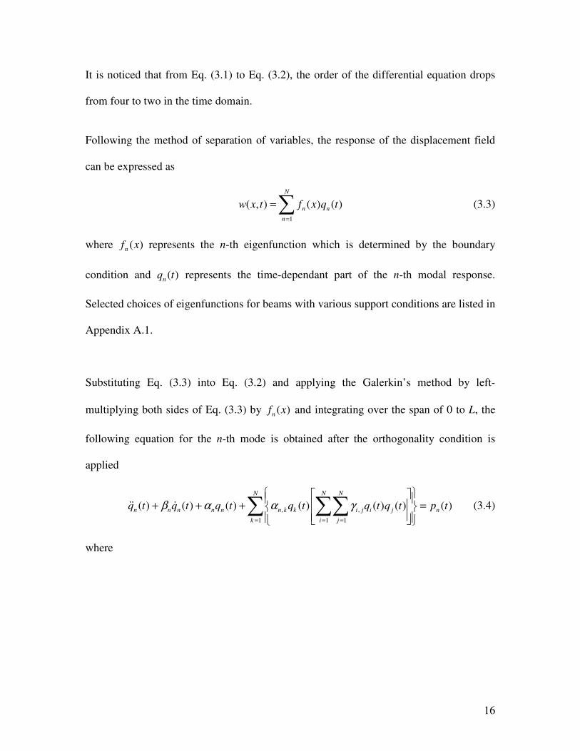
It is noticed that from Eq. (3.1) to Eq. (3.2), the order of the differential equation drops

from four to two in the time domain.

Following the method of separation of variables, the response of the displacement field

can be expressed as

1

( , ) ( ) ( )

N

n n

n

w x t f x q t

=

=∑ (3.3)

where ( )n

f x represents the n-th eigenfunction which is determined by the boundary

condition and ( )n

q t represents the time-dependant part of the n-th modal response.

Selected choices of eigenfunctions for beams with various support conditions are listed in

Appendix A.1.

Substituting Eq. (3.3) into Eq. (3.2) and applying the Galerkin’s method by left-

multiplying both sides of Eq. (3.3) by ( )n

f x and integrating over the span of 0 to L, the

following equation for the n-th mode is obtained after the orthogonality condition is

applied

, ,

1 1 1

( ) ( ) ( ) ( ) ( ) ( ) ( )

N N N

n n n n n n k k i j i j n

k i j

q t q t q t q t q t q t p tβ α α γ= = =

+ + + =

∑ ∑∑ (3.4)

where

17

2

0

''''

02

0

''

0,

2

0

' '

,0

02

0

( )

( ) ( )

( )

( ) ( )

2 ( )

( ) ( )

1( ) ( , ) ( )

( )

n L

n

L

n n nL

n

L

k n

n k L

n

L

i j i j

L

n nL

n

c

A f x dx

EIf x f x dx

A f x dx

EA f x f x dx

AL f x dx

f x f x dx

p t p x t f x dx

A f x dx

βρ

αρ

αρ

γ

ρ

=

=

−=

=

=

∫

∫∫

∫∫

∫

∫∫

(3.5)

Eq. (3.4) can not be solved analytically due to the existence of nonlinear terms. When the

load ( )n

p t is random in nature, the property of interest is the root mean square (R.M.S.)

of the response, which is defined by

[ ]/ 2 22

/ 2

1( )lim

T

x xT

T

x t dtT

σ µ−

→∞

= −∫ (3.6)

where x(t) represents a stationary process that has a constant mean value of x

µ , and T

stands for the period that is under consideration. It can be seen that 2

xσ is also the

variance of the process x(t).

In the equivalent uncoupled linearization method, a linearized equation in the following

form is sought

,( ) ( ) ( ) ( )n n n n n n nq t q t q t p tβ α+ + = (3.7)

where , and n n nβ α represent the damping factor and stiffness of the equivalent system.

18

It can be seen that in Eq. (3.6) different modes of the beam are totally decoupled for each

mode. However, recall that in Eq. (3.4) all the modes are actually coupled through the

nonlinear terms. So it makes more sense if the equivalent equation is written in the linear

coupled format as below

,

1

( ) ( ) ( ) ( )

N

n n n n k n n

k

q t q t q t p tβ α=

+ + =∑ (3.8)

It should be noted that by setting the non-diagonal stiffness terms, , with n k n kα ≠ , to

zero, Eq. (3.8) is the same as the representation of the traditional equivalent linearized

equation as shown in Eq. (3.7).

The difference between Eq.(3.8) and (3.4) is

,

1

, ,

1 1 1

( ) ( ) ( ) ( )

( ) ( ) ( )

N

n k k n n n n n

k

N N N

n k k i j i j

k i j

q t q t q t

q t q t q t

α β β α

α γ

=

= = =

Λ = + − −

−

∑

∑ ∑∑

(3.9)

The goal is to find the optimal values of , and n k nα β of the equivalent linearized system

so that the square of the difference between linear and nonlinear systems is minimalized

in the statistical sense. This requires that

2

2

,

[ ] 0

[ ] 0

n

n k

E

E

β

α

∂Λ =

∂

∂Λ =

∂

(3.10)

where E[•] stands for the mathematical expectation.

19

To demonstrate this procedure in Eq.(3.9) and Eq.(3.10), we look at a simpler case a

beam that is simply supported at both ends, in which Eq.(3.4) is simplified to the

following

2

,1 ,1

1

( ) ( ) ( ( )) ( ) ( )

N

n n n n n k k n n

k

q t q t q t q t p tβ α α +

=

+ + + =∑ (3.11)

where

2 2 4

,1 4

4 4

,1 2 4

0

4

2( ) ( , )sin( )

n

n

n k

L

n

c

A

k n E

L

n EG

L

n xp t p x t

L L

βρ

πα

ρ

π κα

ρ

π

+

=

=

=

= ∫

(3.12)

The equivalent linear system in Eq.(3.8) is used which is listed below again for the sake

of convenience

,

1

( ) ( ) ( ) ( )

N

n n n n k k n

k

q t q t q t p tβ α=

+ + =∑

The difference between Eqs.(3.12) and (3.8) is

2

, ,1 ,1

1 1

( ) ( ( )) ( ) ( ) ( )

N N

n k k n n k k n n n n

k k

q t q t q t q tα α α β β+

= =

Λ = − + + −∑ ∑ (3.13)

Therefore,

20

[ ] [ ] [ ]

2

,

2

, ,1 ,1

1 1

2

, ,1 ,1

1 1

0 [ ]

( ) ( ) ( ( )) ( ) ( )

( ) ( ) ( ) ( ) 3 ( ) ( ) ( )

n k

N N

k n k k n n k k n k

k k

N N

n k n k n n k n k k n k

k k

E

E q t q t E q t q t q t

E q t q t E q t q t E q t E q t q t

α

α α α

α α α

+

= =

+

= =

∂= Λ

∂

= − +

= − +

∑ ∑

∑ ∑

(3.14)

and

2

2

0 [ ]

( ) ( )

n

n n n

E

E q t

β

β β

∂= Λ

∂

= −

(3.15)

which leads to

2

, ,1 ,1

1

3 ( )

N

n k n n k k

k

n n

E q tα α α

β β

+

=

= +

=

∑

(3.16)

In the above derivation, the following relationship and definitions are used under the

assumption that both the load and response follow zero-mean Gaussian distributions

(Soong 2004):

3[ ] [ ] 0

[ ] 0 ( )

n n n n

k n

E q q E q q

E q q k n

= =

= ≠

(3.17)

and

4 2 2

3 2

[ ] 3 [ ]

[ ] 3 [ ] [ ]

n n

k n k n k

E q E q

E q q E q q E q

=

= (3.18)

Another example is given in Appendix A.2 for a beam fixed on one end and simply

supported at the other. In that case, a complete set of quadratic terms maintains and

21

makes the derivation much more tedious. But the idea stays the same. The details are not

discussed here but shown in the Appendix.

Because of the coupling terms in Eq.(3.14), not only the 2[ ]nE q for each mode needs to be

estimated, but also the cross moment terms such as [ ] ( )n kE q q n k≠ . From the frequency

domain analysis, 2[ ]nE q and [ ] ( )n kE q q n k≠ for a linear system are determined by

2 *

*

[ ] ( ) ( ) ( )

[ ] ( ) ( ) ( )

n n n nn

n k n k nk

E q G G S d

E q q G G S d

ω ω ω ω

ω ω ω ω

∞

−∞

∞

−∞

=

=

∫

∫ (3.19)

where )(ωnG is the frequency response function and )(* ωnG is its complex conjugate.

( )nkS ω represents the corresponding power spectral density associated with the n-th and

k-th excitation ( )np t and ( )kp t in the modal equations. For a linear system governed by

Eq. (3.7), )(ωnG takes the form

2

,

1( )

( )n

n n n

Gi

ωα ω β ω

=− +

(3.20)

and ( )nkS ω are defined by

( )0 0

2 2 2

0 0

( ) ( ) ( ) ( )

( ) ( )

( ) ( )

L L

n k

nk PL L

n k

x f x dx x f x dx

S S

A f x dx f x dx

η ηω ω

ρ=∫ ∫

∫ ∫ (3.21)

22

where ( )PS ω represents the power spectral density of the original load ( , )p x t =

( ) ( )x P tη in Eq. (3.1). By definition, the power spectral density is the Fourier transform

of the autocorrelation function ( )R τ of load ( , )p x t :

( ) ( ) i

PS R e dωτω τ τ

∞

−

−∞

= ∫ (3.22)

In the traditional equivalent linearization method, the correlation between different

modes is not considered due to the fact that the final linearized equations are decoupled.

However, numerical simulations indicate that under certain boundary conditions, there

are strong correlations between the responses of different modes in the nonlinear

problem. The value of correlation factor , ( )n k n kρ ≠ is calculated from the following

relationship (under the assumption that both the load and response have zero mean

Gaussian distribution)

, 2 2 2

[ ] ( )

[ ] [ ]

n kn k

n k

E q qn k

E q E qρ = ≠ (3.23)

Finally, the displacement R.M.S. of nonlinear random vibration of the beam can be

obtained after an iteration scheme that is similar to that of the uncoupled linearization

method:

(1) Taking the linear part of Eq.(3.8) only and calculate the first estimate of 2[ ]nE q and

[ ]n k

E q q via Eq.(3.19) to Eq.(3.21) for each of the N modes.

23

(2) The values of 2[ ]nE q and [ ]n k

E q q are then substituted into relationships such as

Eq.(3.16) or Eq.(A.2.12) to find new estimates of parameter , and n k nα β .

(3) The , and n k nα β obtained in step (2) are substituted into Eq.(3.19) to Eq.(3.21) again

to obtain a new estimate of 2[ ]nE q .

(4). Steps (2)-(3) are repeated until a certain converge criterion is achieved after i-th

iterations for all the 2[ ]nE q considered, i.e.,

( ) ( )( )

2 2

1

2

[ ] [ ]

[ ]

n ni i

ni

E q E q

E qε−

−< ( 1, 2, 3 ... n N= )

where ε represent the desired accuracy and usually taken to be 1% or less.

3.2 Effect of Inertia of Rotation and Shear Deformation

In the previous section the nonlinear random vibration of the second order beam is

studied. In that study, the terms associated with the rotary inertia and shear deformation

are neglected. In this section, in order to study how those terms affect the root mean

square response of the beam subjected to random loading, these effects are included in

the governing equation. This results in a fourth-order differential equation in the time

domain. The nonlinear equation of motion for the transverse displacement w(x,t) of an

isotropic beam is expressed in Eq.(3.1)

24

4 2 4 2 4

4 2 2 2 4

2 4 4

2 4 2 2

1

x

w w w E w I wEI c A I

x t t kG x t kG t

w EI w I wN p

x KAG x KAG x t

ρρ ρ

ρ

∂ ∂ ∂ ∂ ∂ + + − + + ∂ ∂ ∂ ∂ ∂ ∂

∂ ∂ ∂− − + = ∂ ∂ ∂ ∂

For a beam simply supported at both ends, (0, ) ( , ) 0w t w L t= = . Assume the solution for

the beam is the summation of the first N modes

sin( ) ( )

N

n

n

n xw q t

L

π=∑ (3.24)

where N represents the total number of modes considered.

Substituting Eq.(3.24) into Eq.(3.1) and applying the Galerkin’s method, the following

equation for the n-th mode is obtained after some lengthy manipulation

2

,1 ,1 ,2

1

2

,3 ,3

1

( ) ( ) ( ) ( )

( ( )) ( ) ( )

N

n n n k k n n N n

k

N

n N n N k k n n

k

q t q q t q t

q t q t p t

α α α

α α

+ +

=

+ + +

=

+ + +

+ + =

∑

∑

(3.25)

where

2 2

,1 2

2 2 4

, 1 4

,2 2

4 4

,3 2 4

2 2 4 2 2 2

,3 2 6

20

( )

4

( )

4

2( ) ( , )sin( )

n

n k

n N

n N

n N k

L

n

AG n E G

I L

k n E

L

c G

I

n EG

L

k n E n EI AGL

I L

G n xp t p x t

L I L

κ π κα

ρ ρ

πα

ρκ

αρ

π κα

ρ

π π κα

ρ

κ πρ

+

+

+

+ +

+= +

=

=

=

+=

= ∫

(3.26)

25

It should be noted that the shear deformation effect and rotary inertia effect are embedded

in terms such as ,1nα and

,2n Nα + in Eq.(3.26).

Notice that in Eq.(3.26) each mode is coupled with the remaining N-1 modes. The

nonlinear coupling makes it impossible to apply the frequency domain analysis to obtain

the root mean square of the displacement response. Now resorting to the equivalent

linearization technique, an equivalent linearized governing equation for each mode in the

following form is sought:

( ) ( ) ( ) ( ) ( )n n n n n n n nq t q t q t q t p tα β γ+ + + = (3.27)

The difference between Eq.(3.25) and (3.27) is

2

,1 ,1 ,2

1

2

,3 ,3

1

( ( )) ( ) ( ) ( )

( ( )) ( )

N

n n n k k n n n N n

k

N

n n N n N k k n

k

q t q t q t

q t q t

α α α β α

γ α α

+ +

=

+ + +

=

Λ = − − + −

+ − −

∑

∑

(3.28)

The goal is to find , , and n n nα β γ so that

2

2

2

[ ] 0

[ ] 0

[ ] 0

n

n

n

E

E

E

α

β

γ

∂Λ =

∂

∂Λ =

∂

∂Λ =

∂

(3.29)

where E[•] stands for the mathematical expectation.

26

Because of the coupling terms in Eq.(3.25), not only the 2[ ]nE q , 2[ ]nE q , and [ ]n n

E q q for

each mode need to be estimated, but also the cross terms such as [ ] ( )n k

E q q n k≠ . They

are obtained from the frequency domain analysis as explained in the following. Recall

that for a linear system, the mean square response is obtained by Eq.(3.19)

2 *( ) ( ) ( )n n n p

G G S dσ ω ω ω ω∞

−∞

= ∫

where ( )nG ω is the frequency response function and )(* ωnG is its complex conjugate.

For a linear system governed by Eq.(3.27), )(ωnG takes the form

4 2

1( )

n e e e

n n n

Gi

ωω α ω γ β ω

=− + +

(3.30)

Furthermore, via random vibration theory, 2[ ]nE q and 2[ ]nE q can be calculated from the

following formulas

( ) ( )

( ) ( )

2

2 24 2

42

2 24 2

1[ ] ( )

[ ] ( )

n ne e e

n n n

n ne e e

n n n

E q S d

E q S d

ω ωω α ω γ β ω

ωω ω

ω α ω γ β ω

∞

−∞

∞

−∞

=− + +

=− + +

∫

∫

(3.31)

where ( )nS ω represents the power spectral density of the excitation ( )np t .

The result for [ ]n nE q q , on the other hand, can be obtained from the autocorrelation

between n

q and n

q :

27

, 2 2 2 2

( ) ( ) ( )

( ) ( ) ( ) ( )n n

n n n nq q

n n n n

E q q E q E q

E q E q E q E qρ

−=

− −

(3.32)

Since the correlation between the displacement and acceleration is unknown, we seek

help from simulation results. After generating 10 series of data with length of 214

,

statistical evaluation of the correlation factor was conducted based on Eq.(3.32).

Numerical simulations were run for different beams with different boundary and loading

conditions. It was found out that the value of n nq qρ

fell into a consistent range of -0.88 to

-0.80. For the purpose of simplicity, the value of -0.88 was used in the analytical analysis.

Eventually, the value of [ ]n nE q q is calculated from the following relationship (under the

assumption that both the response and associated acceleration have zero mean)

2 2 2

,[ ] [ ] [ ]n nn n q q n nE q q E q E qρ=

(3.33)

-0.8 -0.4 0 0.4 0.8Displacement, m

-0.2

-0.1

0

0.1

0.2

Acc

eler

atio

n,

10

6<

m/s

2

Figure 3.2 Correlation between displacement and acceleration for

a typical linear beam (data size: 214

)

28

-0.15 -0.1 -0.05 0 0.05 0.1 0.15Displacement, m

-0.8

-0.4

0

0.4

0.8

Acc

eler

atio

n, 1

06<m

2/s

Figure 3.3 Correlation between displacement and acceleration for

a typical nonlinear beam (data size: 214

)

Solving Eq.(3.29) simultaneously yields the equivalent system parameters nα , nβ and

nγ . During this process, the following statistical properties are applied under the

assumption that both the load and response follow the zero-mean Normal distribution.

3 2

2 2 2 2 2

3

[ ] 3 [ ] [ ]

[ ] [ ] [ ] 2 [ ]

[ ] [ ] 0

[ ] 0

[ ] [ ] [ ] 0 ( )

n n n n n

n n n n n n

n n n n

n n

k n k n k n

E q q E q E q q

E q q E q E q E q q

E q q E q q

E q q

E q q E q q E q q k n

=

= +

= =

=

= = = ≠

(3.34)

29

And, the following definitions are used

2

1

2

2

3

[ ]

[ ]

[ ]

n n

n n

n n n

E E q

E E q

E E q q

=

=

=

(3.35)

Now Eq.(3.29) can be written in the following explicit form:

[ ]

( )

2 2 2

,1 ,1

1

2

,3 ,3

1

,2

2 2

,1 ,1

1

0 [ ] 2 ( ( )) ( )

2 ( )( ( )) ( )

2( ) ( ) ( )

( ) ( )

N

n n n k k n

n k

N

n n n N n N k k n

k

n n N n n

N

n n n n k k n

k

E E q t q t

E q t q t q t

E q t q t

E q t E q t E q

α α αα

γ α α

β α

α α α

+

=

+ + +

=

+

+

=

∂= Λ = − −

∂

+ − −

+ −

= − −

∑

∑

∑

[ ] ( ) [ ]

[ ]

( ) ( )

2

2

, 1 ,3

2 2

,3 ,3

1

2

,1 2 ,1 1 2 , 1 3 ,3

1

( )

2 ( ) ( ) ( ) ( )

( ) ( ) ( ( ) ) 2 ( )

2

n n n n n n N n n

N

n n n N k k n N n n

k

N

n n n n k k n n n n n n N n

k

t

E q t q t E q t q t

E q t q t E q t E q t

E E E E E

α γ α

α α

α α α α γ α

+ +

+ + + +

=

+ + +

=

+ + −

− +

= − − + + −

∑

∑

3

3 ,3 1 ,3 1

1

( ) 2

N

n n N k k n N n n

k

E E Eα α+ + + +

=

− +

∑ (3.36)

2

2

,2

0 [ ]

( ) ( )

n

n n N n

E

E q t

β

β α +

∂= Λ

∂

= −

(3.37)

30

( )

( ) [ ]

[ ] [ ]

2

2 2

,3 ,3

1

2 2

,3 ,1

2 2

,1 , 1

1

,3

0 [ ]

( ) ( ( ) )

2 ( ) ( ) ( ) ( )

( ( ) ) ( ) ( ) 2 ( ) ( ) ( )

n

N

n n N n n N k k

k

n N n n n n n n n

N

n k k n n n n n n n

k

n n

E

E q t E q t

E q t E q t E q t q t

E q t E q t q t E q t E q t q t

γ

γ α α

α α α

α α

γ α

+ + +

=

+ +

+ +

=

∂= Λ

∂

= − −

+ + −

− −

= −

∑

∑

( )

( )

1 ,3 1 ,3 1 1

1

,1 3 ,1 1 3 , 1 1 3

1

( ) 2

( ) 2

N

N n n N k k n N n n n

k

N

n n n n k k n n n n n

k

E E E E

E E E E E

α α

α α α α

+ + + + +

=

+ +

=

− +

+ − − −

∑

∑

(3.38)

From Eq.(3.32)-Eq.(3.34), we have

,1 ,1 1

1

,2

, 1 3 ,3 ,3 1 ,3 1

1

( )

2 2

N

n n n k k

k

n n N

N

n n n n n N n n N n n N k k

k

E

E E E

α α α

β α

γ α α α α

+

=

+

+ + + + + +

=

= +

=

= + + +

∑

∑

(3.39)

It is recalled that based on the analysis in the past, the damping term in the equivalent

system would stay the same because there is no nonlinear term in the damping coefficient

in Eq.(3.25). The results in Eq.(3.39) also verifies that conclusion.

Finally, the root mean square of nonlinear random vibration of the fourth-order beam can

be obtained after an iteration scheme that is described as follows

31

(1) Taking the linear part of Eq.(3.25) only and calculate the first estimate of 2[ ]nE q ,

2[ ]nE q , and [ ]n nE q q via Eqs.(3.30) to (3.33) for each of the N modes.

(2) The values of 2[ ]nE q , 2[ ]nE q , and [ ]n nE q q are then substituted into Eq.(3.39) to find

new estimates of parameter , and n n nα β γ .

(3) The , and n n nα β γ obtained in step (2) are substituted into Eq.(3.31) again to obtain a

new estimate of 2[ ]nE q .

(4). Steps (2)-(3) are repeated until a certain converge criterion is achieved after k-th

iterations for all the 2[ ]nE q considered, i.e.,

( ) ( )

( )2 2

1

2

[ ] [ ]

[ ]

n nk k

nk

E q E q

E qε−

−< ( 1, 2, 3 ... n N= )

where ε represent the desired accuracy and usually taken to be 1% or less.

3.3 Numerical Results

Numerical studies are conducted using the procedures discussed above. The beams used

in the study have the same cross section aspect ratio (height/width = 2) but different

length/thickness ratios. The length of the beam is fixed at L = 1 m for the purpose of

simplicity, and the beam is made from material that has a modulus of elasticity E = 70

GPa, and a density ρ = 3000 kg/m3. A damping factor c = 100 N⋅s/m

2 is used.

32

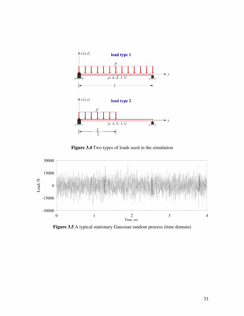
Two types of loads are considered: a uniformly distributed pressure load over the whole

span of the beam and a half-uniformly distributed pressure load over the left half span of

the beam, as shown in Figure 3.4. Both loads have the spectrum of that of a band-limited

white noise. Figure 3.5 shows the load history during a span of four seconds. The power

spectral density of these two loads is plotted in Figure 3.7. One of the key reasons to

choose these two loads is that they represent the symmetric and unsymmetrical type of

loading, respectively. As a result, if the boundary conditions are also symmetric, only the

odd modes will be excited under symmetric loading condition, otherwise all the modes

will be excited.

Results from the numerical study aim at addressing the following issues:

• difference between the linear and nonlinear random vibration analysis

• advantage of the equivalent coupled linearization method over the equivalent

uncoupled linearization method, if there is any

• effects of rotary inertia and shear deformation on the response of the beam under

random excitation

• impact of different boundary or loading conditions on the response of the beam

33

Figure 3.4 Two types of loads used in the simulation

0 1 2 3 4Time, sec

-30000

-15000

0

15000

30000

Load, N

Figure 3.5 A typical stationary Gaussian random process (time domain)

34

-24000 -16000 -8000 0 8000 16000 24000Load, N

0

0.04

0.08

0.12

0.16

Rel

ativ

e fr

equ

ency

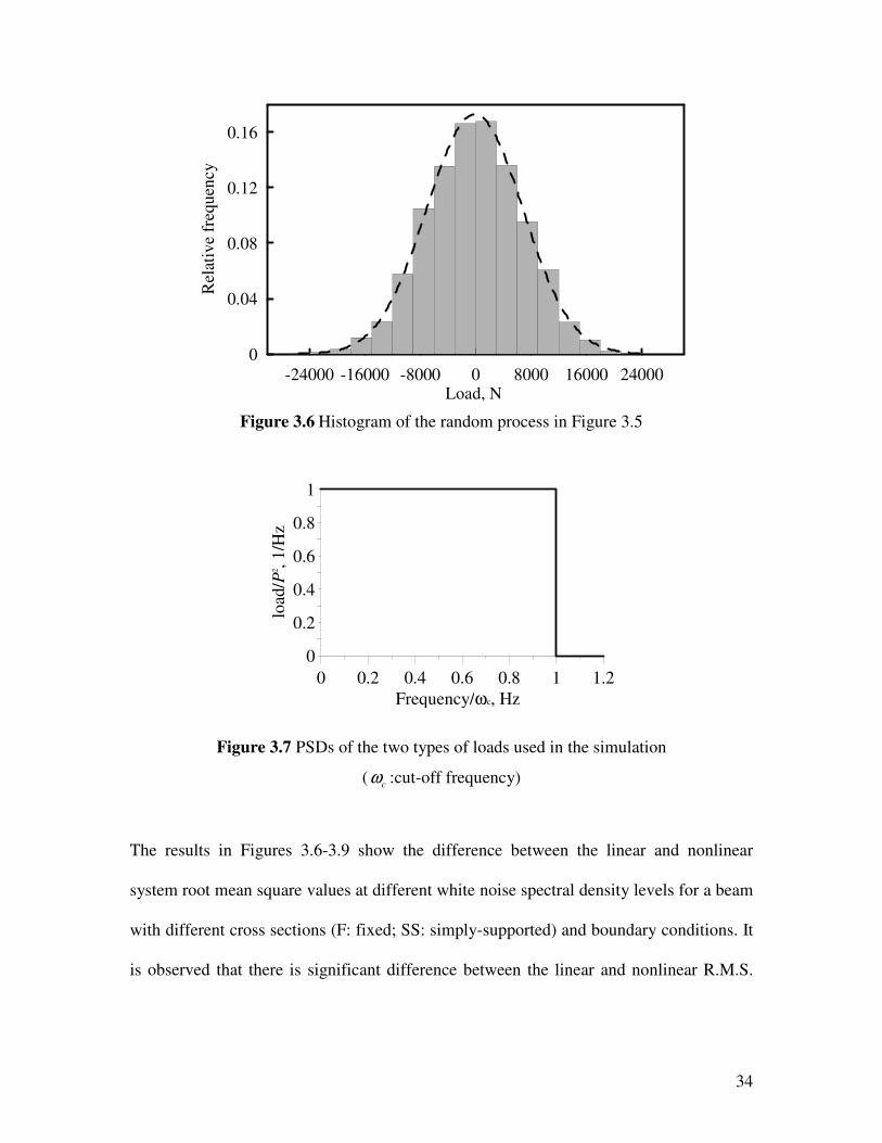
Figure 3.6 Histogram of the random process in Figure 3.5

0 0.2 0.4 0.6 0.8 1 1.2

Frequency/ωc, Hz

0

0.2

0.4

0.6

0.8

1

load

/P2,

1/H

z

Figure 3.7 PSDs of the two types of loads used in the simulation

(c

ω :cut-off frequency)

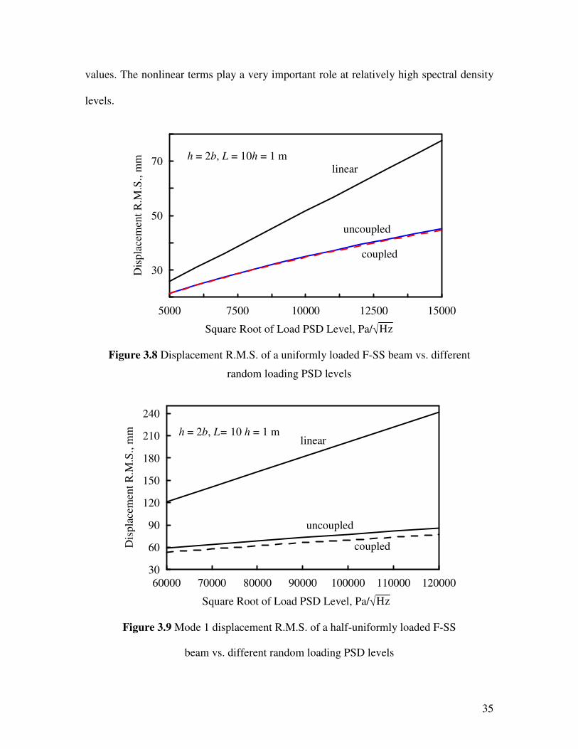
The results in Figures 3.6-3.9 show the difference between the linear and nonlinear

system root mean square values at different white noise spectral density levels for a beam

with different cross sections (F: fixed; SS: simply-supported) and boundary conditions. It

is observed that there is significant difference between the linear and nonlinear R.M.S.

35

values. The nonlinear terms play a very important role at relatively high spectral density

levels.

5000 7500 10000 12500 15000

Square Root of Load PSD Level, Pa/√Hz

30

50

70

Dis

pla

cem

ent

R.M

.S.,

mm

coupled

uncoupled

linear

h = 2b, L = 10h = 1 m

Figure 3.8 Displacement R.M.S. of a uniformly loaded F-SS beam vs. different

random loading PSD levels

60000 70000 80000 90000 100000 110000 120000


30

60

90

120

150

180

210

240

Dis

pla

cem

ent

R.M

.S.,

mm

linear

coupled

h = 2b, L= 10 h = 1 m

uncoupled

Figure 3.9 Mode 1 displacement R.M.S. of a half-uniformly loaded F-SS

beam vs. different random loading PSD levels

36

60000 70000 80000 90000 100000 110000 120000


30

60

90

120

Dis

pla

cem

ent

R.M

.S.,

mm

linear

coupled

uncoupled

h = 2b, L= 10 h = 1 m

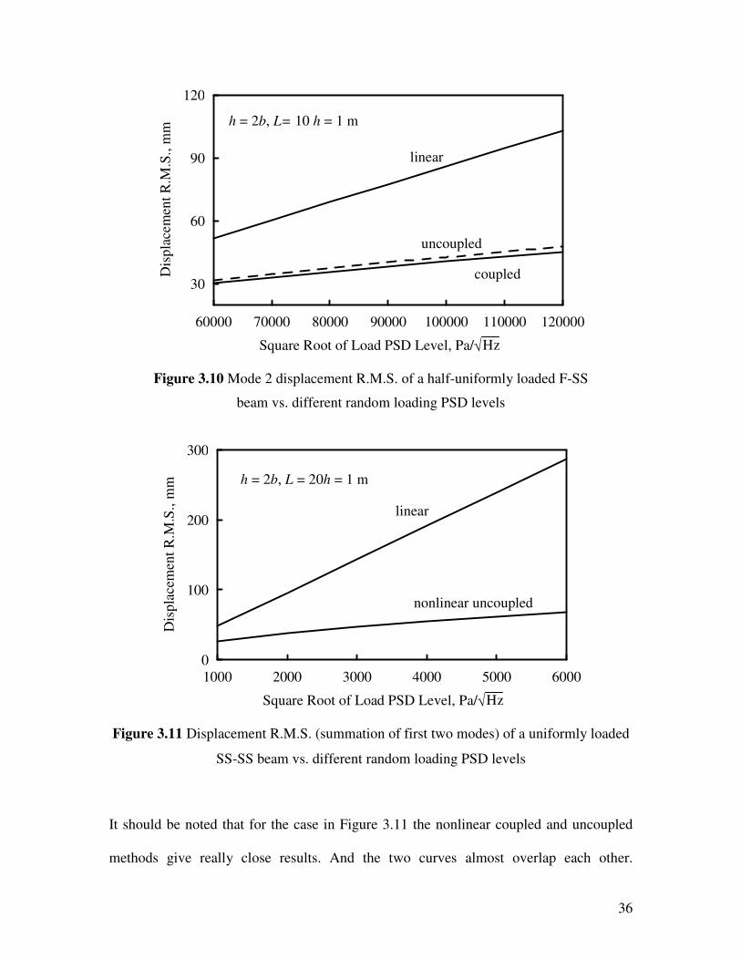
Figure 3.10 Mode 2 displacement R.M.S. of a half-uniformly loaded F-SS

beam vs. different random loading PSD levels

1000 2000 3000 4000 5000 6000


0

100

200

300

Dis

pla

cem

ent

R.M

.S.,

mm

linear

nonlinear uncoupled

h = 2b, L = 20h = 1 m

Figure 3.11 Displacement R.M.S. (summation of first two modes) of a uniformly loaded

SS-SS beam vs. different random loading PSD levels

It should be noted that for the case in Figure 3.11 the nonlinear coupled and uncoupled

methods give really close results. And the two curves almost overlap each other.

37

Therefore, only the nonlinear coupled results are shown and referred to as “nonlinear” for

the purpose of simplicity.

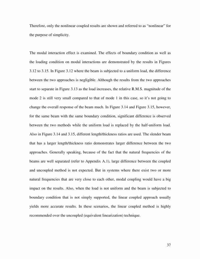
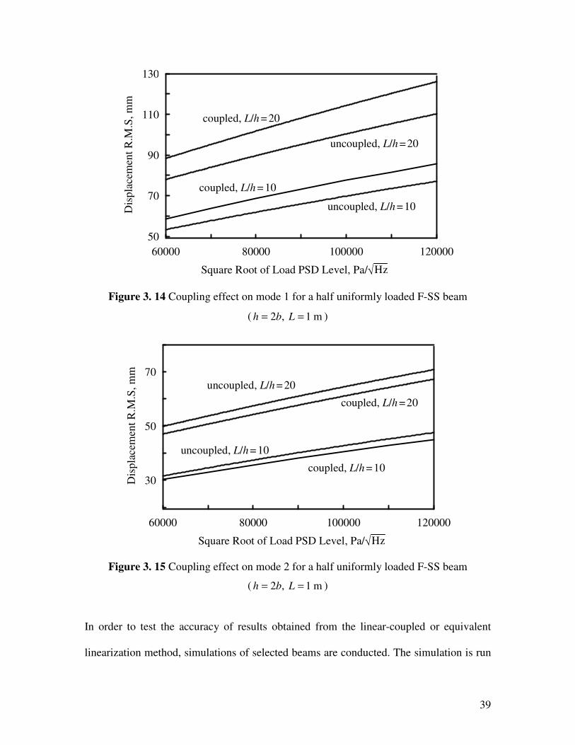
The modal interaction effect is examined. The effects of boundary condition as well as

the loading condition on modal interactions are demonstrated by the results in Figures

3.12 to 3.15. In Figure 3.12 where the beam is subjected to a uniform load, the difference

between the two approaches is negligible. Although the results from the two approaches

start to separate in Figure 3.13 as the load increases, the relative R.M.S. magnitude of the

mode 2 is still very small compared to that of mode 1 in this case, so it’s not going to

change the overall response of the beam much. In Figure 3.14 and Figure 3.15, however,

for the same beam with the same boundary condition, significant difference is observed

between the two methods while the uniform load is replaced by the half-uniform load.

Also in Figure 3.14 and 3.15, different length/thickness ratios are used. The slender beam

that has a larger length/thickness ratio demonstrates larger difference between the two

approaches. Generally speaking, because of the fact that the natural frequencies of the

beams are well separated (refer to Appendix A.1), large difference between the coupled

and uncoupled method is not expected. But in systems where there exist two or more

natural frequencies that are very close to each other, modal coupling would have a big

impact on the results. Also, when the load is not uniform and the beam is subjected to

boundary condition that is not simply supported, the linear coupled approach usually

yields more accurate results. In these scenarios, the linear coupled method is highly

recommended over the uncoupled (equivalent linearization) technique.

38

uncoupled

coupled

8000 12000 16000 20000 24000


20

30

40

50

60

Dis

pla

cem

ent

R.M

.S,

mm h = 2b, L = 10h = 1 m

Figure 3.12 Coupling effect on mode 1 for a uniformly loaded F-SS beam

uncoupled

coupled

8000 12000 16000 20000 24000


0

1

2

3

4

5

Dis

pla

cem

ent

R.M

.S,

mm h = 2b, L = 10h = 1 m

Figure 3.13 Coupling effect on mode 2 for a uniformly loaded F-SS beam

39

60000 80000 100000 120000


50

70

90

110

130

Dis

pla

cem

ent

R.M

.S,

mm

uncoupled, L/h = 10

coupled, L/h = 10

uncoupled, L/h = 20

coupled, L/h = 20

Figure 3. 14 Coupling effect on mode 1 for a half uniformly loaded F-SS beam

( 2 , 1 mh b L= = )

60000 80000 100000 120000


30

50

70

Dis

pla

cem

ent

R.M

.S,

mm

uncoupled, L/h = 10

coupled, L/h = 10

uncoupled, L/h = 20

coupled, L/h = 20

Figure 3. 15 Coupling effect on mode 2 for a half uniformly loaded F-SS beam

( 2 , 1 mh b L= = )

In order to test the accuracy of results obtained from the linear-coupled or equivalent

linearization method, simulations of selected beams are conducted. The simulation is run

40

twenty times with a sample size of 214

and the mean values are listed in Table 3.1 to

Table 3.4 along with the analytical predictions. The time step is chosen to be 1/c

ω (c

ω :

cut-off frequency) second to make sure the second mode frequency is well covered. In

other words, the Nyquist frequency condition is satisfied.

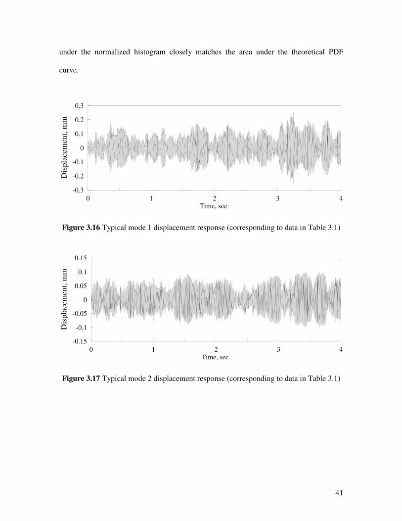
Figure 3.16 and Figure 3.17 show the displacement responses of first two modes of a

fixed-simply supported beam under half-uniform load (refer to Table 3.1 for beam

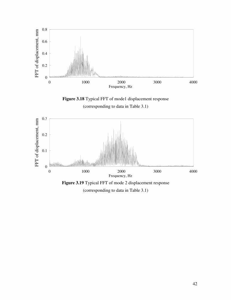
geometry and loading/boundary conditions) during a four-second span. In Figure 3.18 to

Figure 3.19, the FFT (fast Fourier transform) plots of the responses of the two modes are

displayed. The peaks in the figures indicate that there are inherent harmonic components

in the response. The peak positions in these two figures indicate that the mode 1 has

significant influence on the mode 2 response. On the other hand, the influence of mode

two on mode 1 is negligible even though the R.M.S. values of the first two modes are on

the same order (as is shown in Table 3.1).

The normalized histogram of the first two modes of one nonlinear beam response is

shown in Figure 3.20 and 3.21. The corresponding theoretical probability density

functions (PDF) of normal distribution based on zero mean and calculated R.M.S. value

are also presented in dashed lines. Recall that an assumption is made in the very

beginning of this study that the response for a linear system subjected to normally

distributed load also follows normal distribution. Although for nonlinear system the

shape of the histogram may not follow that of a normal distribution perfectly, the area

41

under the normalized histogram closely matches the area under the theoretical PDF

curve.

0 1 2 3 4Time, sec

-0.3

-0.2

-0.1

0

0.1

0.2

0.3

Dis

pla

cem

ent,

mm


0 1 2 3 4Time, sec

-0.15

-0.1

-0.05

0

0.05

0.1

0.15

Dis

pla

cem

ent,

mm


42

0 1000 2000 3000 4000Frequency, Hz

0

0.2

0.4

0.6

0.8

FF

T o

f dis

pla

cem

ent,

mm

Figure 3.18 Typical FFT of mode1 displacement response

(corresponding to data in Table 3.1)

0 1000 2000 3000 4000Frequency, Hz

0

0.1

0.2

0.3

FF

T o

f dis

pla

cem

ent,

mm

Figure 3.19 Typical FFT of mode 2 displacement response

(corresponding to data in Table 3.1)

43

-0.24 -0.16 -0.08 0 0.08 0.16 0.24Displacement, m

0

0.04

0.08

0.12

Rel

ativ

e fr

equ

ency

Figure 3.20 Histogram of mode 1 displacement response

(corresponding to data in Table 3.1, sample size: 214

)

-0.12 -0.08 -0.04 0 0.04 0.08 0.12Displacement, m

0

0.04

0.08

0.12

Rel

ativ

e fr

equ

ency

Figure 3.21 Histogram of mode 2 displacement response

(corresponding to data in Table 3.1, sample size: 214

)

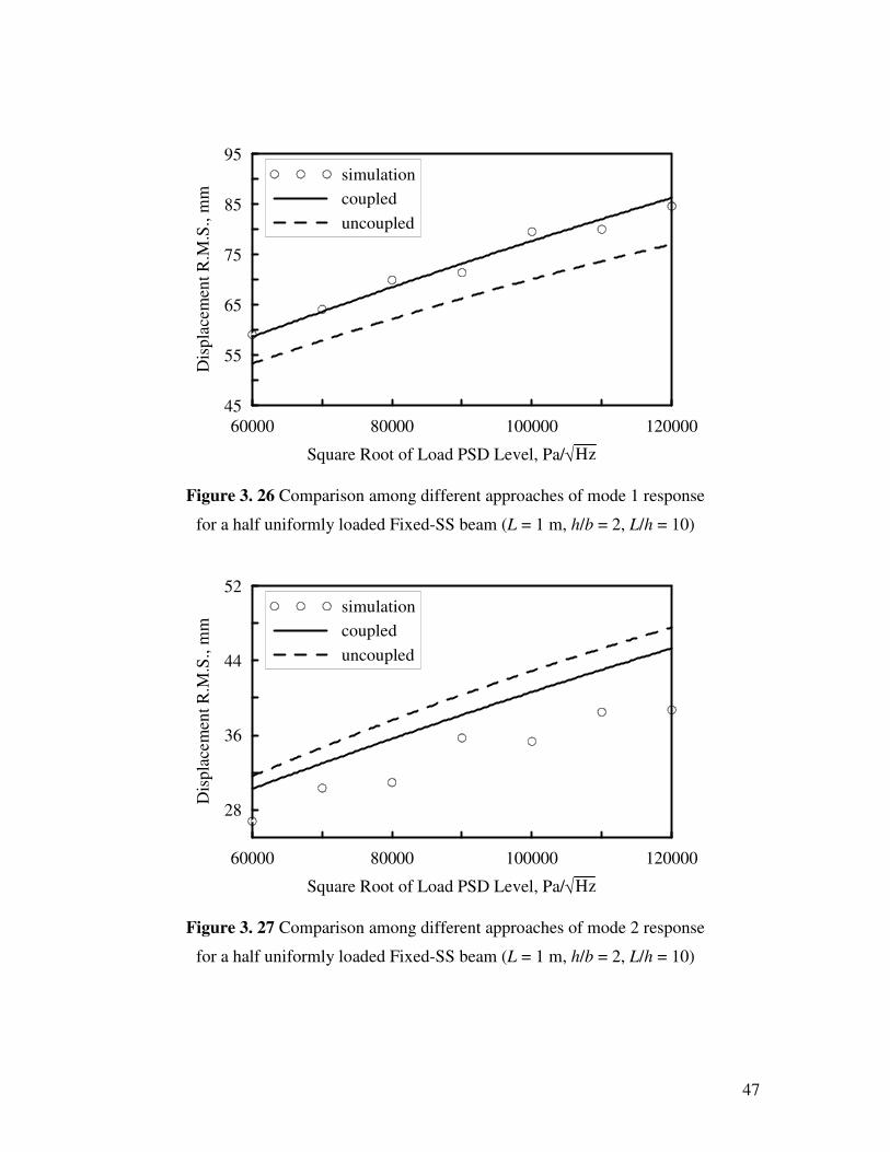
Good agreement between the analytical approach and simulation is found. For the mode 1

results in Table 3.1 and Table 3.2, the analytical predictions from linear-coupled

44

approach are much closer to simulation results than the values from uncoupled approach

are. More results are demonstrated in Figures 3.22 to 3.29 for two Fixed-SS beams

subjected to various load PSD levels. In these figures the beam has a different cross

section from those in Table 3.1 and 3.2. It can be seen that for both mode 1 and mode 2,

the linear coupled method yields closer results to those obtained from simulations. It

should be noted that the beam examined in all these figures is asymmetrically supported

and loaded.

Table 3.1 Response of a beam (mm) with F-SS boundary condition and subjected to half

uniform load (load PSD = 100000 Pa2/Hz, 2 , 10 1 mh b L h= = = )

simulation linear coupled uncoupled & w/ corre. uncoupled & w/o corre.

mode1 77.6 78.1 70.1 69.5

mode2 31.4 40.9 42.9 42.6

Table 3.2 Response of a beam with F-SS boundary condition and subjected to half

uniform load (load PSD = 100000 Pa2/Hz, 2 , 20 1 mh b L h= = = )


mode1 113.1 114.2 100.2 100.2

mode2 54.8 60.9 64.3 64.3

Table 3.3 Response of a beam (mm) with F-SS boundary condition and subjected to

uniform load (load PSD = 10000 Pa2/Hz, 2 , 12.5 1 mh b L h= = = )


mode1 40.3 42.3 41.6 41.6

mode2 4.39 2.63 2.05 2.05

Tabel 3.4 Response of a beam (mm) with F-Fixed boundary condition and subjected to

half uniform load (load PSD = 100000 Pa2/Hz, 2 , 12.5 1 mh b L h= = = )


mode1 85.2 86.7 87.4 86.7

mode2 45.0 44.3 44.6 44.3

45

60000 80000 100000 120000


45

55

65

75D

isp

lace

men

t R

.M.S

., m

m

simulation

coupled

uncoupled

Figure 3.22 Comparison among different approaches of mode 1 response

for a half uniformly loaded Fixed-S (L = 1 m, h/b = 1, L/h = 10)

60000 80000 100000 120000


20

28

36

44

Dis

pla

cem

ent

R.M

.S.,

mm

simulation

coupled

uncoupled


for a half uniformly loaded Fixed-SS beam (L = 1 m, h/b = 1, L/h = 10)

46

60000 80000 100000 120000


70

90

110

Dis

pla

cem

ent

R.M

.S.,

mm

simulation

coupled

uncoupled



60000 80000 100000 120000


35

45

55

65

Dis

pla

cem

ent

R.M

.S.,

mm

simulation

coupled

uncoupled

Figure 3. 25 Comparison among different approaches of mode 2 response


47

60000 80000 100000 120000


45

55

65

75

85

95

Dis

pla

cem

ent

R.M

.S.,

mm

simulation

coupled

uncoupled



60000 80000 100000 120000


28

36

44

52

Dis

pla

cem

ent

R.M

.S.,

mm

simulation

coupled

uncoupled



48

60000 80000 100000 120000


70

90

110

130

Dis

pla

cem

ent

R.M

.S.,

mm

simulation

coupled

uncoupled



60000 80000 100000 120000


45

55

65

75

Dis

pla

cem

ent

R.M

.S.,

mm

simulation

coupled

uncoupled



49

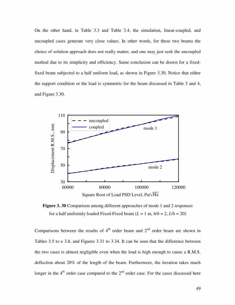
On the other hand, in Table 3.3 and Table 3.4, the simulation, linear-coupled, and

uncoupled cases generate very close values. In other words, for these two beams the

choice of solution approach does not really matter, and one may just seek the uncoupled

method due to its simplicity and efficiency. Same conclusion can be drawn for a fixed-

fixed beam subjected to a half uniform load, as shown in Figure 3.30. Notice that either

the support condition or the load is symmetric for the beam discussed in Table 3 and 4,

and Figure 3.30.

60000 80000 100000 120000


30

50

70

90

110

Dis

pla

cem

ent

R.M

.S.,

mm

uncoupled

coupled mode 1

mode 2

Figure 3. 30 Comparison among different approaches of mode 1 and 2 responses

for a half uniformly loaded Fixed-Fixed beam (L = 1 m, h/b = 2, L/h = 20)

Comparisons between the results of 4th

order beam and 2nd

order beam are shown in

Tables 3.5 to e 3.8, and Figures 3.31 to 3.34. It can be seen that the difference between

the two cases is almost negligible even when the load is high enough to cause a R.M.S.

deflection about 20% of the length of the beam. Furthermore, the iteration takes much

longer in the 4th

order case compared to the 2nd

order case. For the cases discussed here

50

(refer to data presented in Table 3.5 to Table 3.8), the effect of shear deformation and

rotary inertia effects on the random vibration of nonlinear beam is not significant.



order beam

(SS-SS boundary condition with uniform load, 2 , 10 1 mh b L h= = = )

Square root of mode 1 R.M.S., mm mode 2 R.M.S., mm

load PSD, Pa/Hz1/2

2nd order 4th order % diff 2nd order 4th order % diff

60000 150.4 150.7 0.1% 18.4 17.9 -2.6%

70000 162.6 163.1 0.3% 20.5 19.9 -2.7%

80000 174.0 174.8 0.5% 22.4 21.8 -2.7%

90000 186.4 185.7 -0.4% 24.4 23.6 -3.2%

100000 196.6 196.1 -0.2% 26.1 25.3 -3.1%



order beam

(SS-SS boundary condition with half-uniform load, 2 , 10 1 mh b L h= = = )

Square root of mode 1 R.M.S., mm mode 2 R.M.S., mm

load PSD, Pa/Hz1/2

2nd order 4th order % diff 2nd order 4th order % diff

60000 105.5 104.7 -0.7% 10.9 10.7 -1.9%

70000 114.3 113.6 -0.6% 12.3 12.1 -2.1%

80000 122.3 121.9 -0.4% 13.7 13.3 -2.3%

90000 130.0 129.7 -0.2% 14.9 14.6 -2.4%

100000 137.1 137.0 -0.1% 16.2 15.7 -2.5%



order beam (F-SS boundary condition with half-uniform load, 2 , 10 1 mh b L h= = = )

Square root of mode 1 R.M.S., mm

load PSD, Pa/Hz1/2

2nd order w/o C.P. 2nd order w/ C.P. 4th order

60000 53.3 58.7 60.9

70000 57.6 63.7 66.1

80000 61.8 68.6 71.1

90000 66.3 73.2 75.6

100000 69.5 77.6 79.8

110000 73.6 81.7 84.0

120000 77.0 85.6 87.9

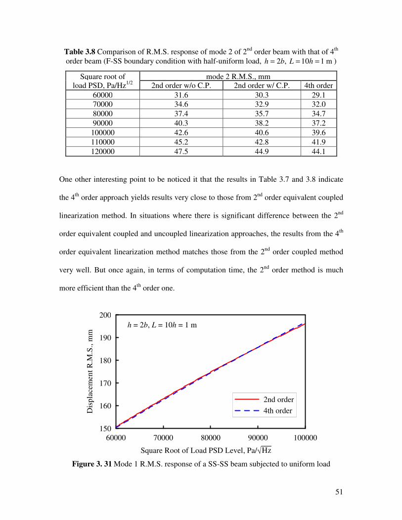
51



order beam (F-SS boundary condition with half-uniform load, 2 , 10 1 mh b L h= = = )

Square root of mode 2 R.M.S., mm load PSD, Pa/Hz

1/2 2nd order w/o C.P. 2nd order w/ C.P. 4th order

60000 31.6 30.3 29.1

70000 34.6 32.9 32.0

80000 37.4 35.7 34.7

90000 40.3 38.2 37.2

100000 42.6 40.6 39.6

110000 45.2 42.8 41.9

120000 47.5 44.9 44.1

One other interesting point to be noticed it that the results in Table 3.7 and 3.8 indicate

the 4th

order approach yields results very close to those from 2nd

order equivalent coupled

linearization method. In situations where there is significant difference between the 2nd

order equivalent coupled and uncoupled linearization approaches, the results from the 4th

order equivalent linearization method matches those from the 2nd

order coupled method

very well. But once again, in terms of computation time, the 2nd

order method is much

more efficient than the 4th

order one.

60000 70000 80000 90000 100000


150

160

170

180

190

200

Dis

pla

cem

ent

R.M

.S.,

mm

2nd order

4th order

h = 2b, L = 10h = 1 m

Figure 3. 31 Mode 1 R.M.S. response of a SS-SS beam subjected to uniform load

52

60000 70000 80000 90000 100000


16

20

24

28

Dis

pla

cem

ent

R.M

.S.,

mm

2nd order

4th order

h = 2b, L = 10h = 1 m

Figure 3. 32 Mode 2 R.M.S. response of a SS-SS beam subjected to uniform load

60000 80000 100000 120000


50

60

70

80

90

Dis

pla

cem

ent

R.M

.S.,

mm

2nd order coupled

4th order

2nd order uncoupled

h = 2b, L = 10h = 1 m

Figure 3. 33 Mode 1 R.M.S. response of a F-SS beam subjected to half-uniform load

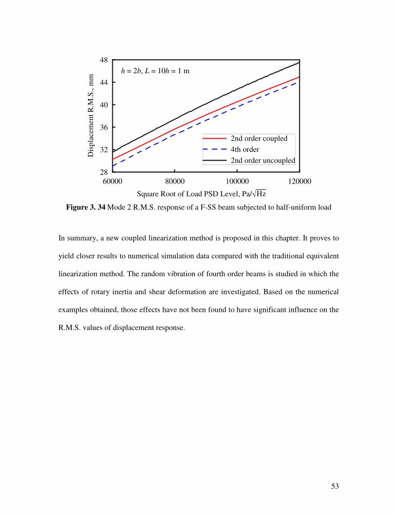
53

60000 80000 100000 120000


28

32

36

40

44

48

Dis

pla

cem

ent

R.M

.S.,

mm

2nd order coupled

4th order

2nd order uncoupled

h = 2b, L = 10h = 1 m

Figure 3. 34 Mode 2 R.M.S. response of a F-SS beam subjected to half-uniform load

In summary, a new coupled linearization method is proposed in this chapter. It proves to

yield closer results to numerical simulation data compared with the traditional equivalent

linearization method. The random vibration of fourth order beams is studied in which the

effects of rotary inertia and shear deformation are investigated. Based on the numerical

examples obtained, those effects have not been found to have significant influence on the

R.M.S. values of displacement response.

54

Chapter 4. Nonlinear Random Vibration of

Composite Plates

In this chapter the techniques discussed in Chapter 3 are extended to solve the nonlinear

random vibration problem of composite plates. Classical plate theory (CPT) and the first

order shear deformation theory (FSDT) in both linear and nonlinear forms are used to

obtain the R.M.S. response of the transverse displacement. The difference between the

two theories is demonstrated through numerical examples. Geometric nonlinear effect is

examined. Temperature effects on the R.M.S. values of both displacement and stress

components are also studied.

4.1 Governing Equations

Figure 4.1 (without bending moments) and Figure 4.2 (bending moments only) show the

free body diagrams of a rectangular plate element in general loading condition.

55

Figure 4.1 Free body diagram of a rectangular plate element (without bending moments)

Figure 4.2 Free body diagram of a rectangular plate element (bending moments only)

56

The equations of equilibrium (without in-plane loading, damping terms not shown for the

purpose of simplicity) can be obtained by the principle of virtual work. The detailed

derivation can be found in Appendix B.

2 2

00 12 2

2 2

00 12 2

0 0 0 0

0 0 0 0

TTxy xyxx xx

T T

xy yy xy yy

y T Txxx xy xx xy

T T

xy yy xy yy

N NN N uI I

x y x y t t

N N N N vI I

x y x y t t

VV w w w wN N N N

x y x x y x y

w w w wN N N N

y x y y y

φ

ψ

∂ ∂∂ ∂ ∂ ∂+ + + = +

∂ ∂ ∂ ∂ ∂ ∂

∂ ∂ ∂ ∂ ∂ ∂+ + + = +

∂ ∂ ∂ ∂ ∂ ∂

∂ ∂ ∂ ∂ ∂ ∂∂+ + + + + ∂ ∂ ∂ ∂ ∂ ∂ ∂

∂ ∂ ∂ ∂∂+ + + +∂ ∂ ∂ ∂ ∂

2

00 2

22

02 12 2

22

02 12 2

TTxy xyxx xx

x

T T

xy yy xy yy

y

wI

t

M MM M uV I I

x y x y t t

M M M M vV I I

x y x y t t

φ

ψ

∂= ∂

∂ ∂∂ ∂ ∂∂+ + + − = +

∂ ∂ ∂ ∂ ∂ ∂

∂ ∂ ∂ ∂ ∂∂+ + + − = +

∂ ∂ ∂ ∂ ∂ ∂

(4.1)

where dzzIi

h

hi ∫−=

2/

2/ρ (i = 1, 2, 3), and the force resultants N’s and moment resultants

M’s can be obtained from the relationship

2

20

11 12 16 11 12 16 20

12 22 26 12 22 26 2

0

16 26 66 16 26 66 2

11

2

xx xx xx

yy yy yy

xy xy xy

xx

yy

xy

w

xN A A A T B B B

wN A A A T B B B

yN A A A T B B B

w

x y

M B

M

M

ε α

ε α

γ α

∂

∂ − ∆ ∂ = − ∆ + ∂ − ∆ ∂

∂ ∂

=

2

20

12 16 11 12 16 20

12 22 26 12 22 26 2

0

16 26 66 16 26 66 2

2

xx xx

yy yy

xy xy

w

xB B T D D D

wB B B T D D D

yB B B T D D D

w

x y

ε α

ε α

γ α

∂

∂ − ∆ ∂ − ∆ + ∂ − ∆ ∂

∂ ∂

(4.2)

and

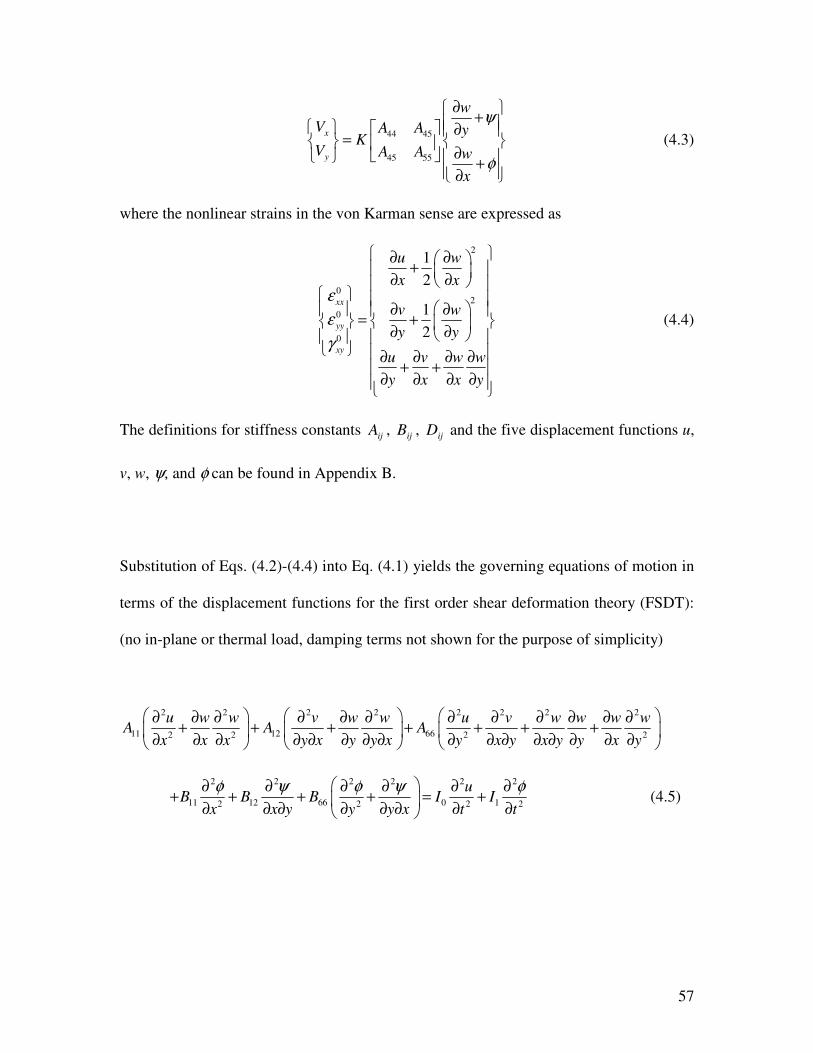
57

44 45

45 55

x

y

w

V A A yK

V A A w

x

ψ

φ

∂ + ∂ =

∂ + ∂

(4.3)

where the nonlinear strains in the von Karman sense are expressed as

2

02

0

0

1

2

1

2

xx

yy

xy

u w

x x

v w

y y

u v w w

y x x y

ε

ε

γ

∂ ∂ + ∂ ∂

∂ ∂ = + ∂ ∂

∂ ∂ ∂ ∂+ +

∂ ∂ ∂ ∂

(4.4)

The definitions for stiffness constants ijA , ijB , ijD and the five displacement functions u,

v, w, ψ, and φ can be found in Appendix B.

Substitution of Eqs. (4.2)-(4.4) into Eq. (4.1) yields the governing equations of motion in

terms of the displacement functions for the first order shear deformation theory (FSDT):

(no in-plane or thermal load, damping terms not shown for the purpose of simplicity)

2 2 2 2 2 2 2 2

11 12 662 2 2 2

u w w v w w u v w w w wA A A

x x x y x y y x y x y x y y x y

∂ ∂ ∂ ∂ ∂ ∂ ∂ ∂ ∂ ∂ ∂ ∂+ + + + + + + ∂ ∂ ∂ ∂ ∂ ∂ ∂ ∂ ∂ ∂ ∂ ∂ ∂ ∂ ∂ ∂

2 2 2 2 2 2

11 12 66 0 12 2 2 2

uB B B I I

x x y y y x t t

φ ψ φ ψ φ ∂ ∂ ∂ ∂ ∂ ∂+ + + + = + ∂ ∂ ∂ ∂ ∂ ∂ ∂ ∂

(4.5)

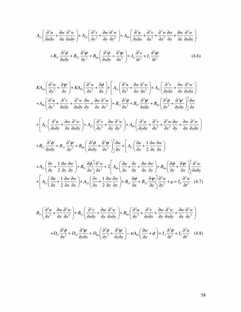
58

2 2 2 2 2 2 2 2

12 22 662 2 2 2


x y x x y y y y y x x x y x y x

∂ ∂ ∂ ∂ ∂ ∂ ∂ ∂ ∂ ∂ ∂ ∂+ + + + + + + ∂ ∂ ∂ ∂ ∂ ∂ ∂ ∂ ∂ ∂ ∂ ∂ ∂ ∂ ∂ ∂

2 2 2 2 2 2

12 22 66 0 12 2 2 2

vB B B I I

x y y x y x t t

φ ψ φ ψ ψ ∂ ∂ ∂ ∂ ∂ ∂+ + + + = + ∂ ∂ ∂ ∂ ∂ ∂ ∂ ∂

(4.6)

2 2 2 2 2 2

44 55 11 122 2 2 2

w w u w w v w wKA KA A A

y y x x x x x y x y y x

ψ φ ∂ ∂ ∂ ∂ ∂ ∂ ∂ ∂ ∂ ∂+ + + + + + + ∂ ∂ ∂ ∂ ∂ ∂ ∂ ∂ ∂ ∂ ∂ ∂

2 2 2 2 2 2 2 2

66 11 12 662 2 2 2

u v w w w w wA B B B

y x y x y y x y x x y y y x x

φ ψ φ ψ ∂ ∂ ∂ ∂ ∂ ∂ ∂ ∂ ∂ ∂ ∂+ + + + + + + + ∂ ∂ ∂ ∂ ∂ ∂ ∂ ∂ ∂ ∂ ∂ ∂ ∂ ∂ ∂

2 2 2 2 2 2 2 2

12 22 662 2 2 2



∂ ∂ ∂ ∂ ∂ ∂ ∂ ∂ ∂ ∂ ∂ ∂+ + + + + + + + ∂ ∂ ∂ ∂ ∂ ∂ ∂ ∂ ∂ ∂ ∂ ∂ ∂ ∂ ∂ ∂

2 2 2 2

12 22 66 112 2

1

2

w u w wB B B A

x y y x y x y x x x

φ ψ φ ψ ∂ ∂ ∂ ∂ ∂ ∂ ∂ ∂ + + + + + + ∂ ∂ ∂ ∂ ∂ ∂ ∂ ∂ ∂ ∂

2 2

12 11 66 662

12

2

v w w w u v w w wA B A B

y y y x x x y x y y x x y

φ φ ψ ∂ ∂ ∂ ∂ ∂ ∂ ∂ ∂ ∂ ∂ ∂ ∂+ + + + + + + + ∂ ∂ ∂ ∂ ∂ ∂ ∂ ∂ ∂ ∂ ∂ ∂ ∂

2 2

12 22 12 22 02 2

1 1

2 2

u w w v w w w wA A B B q I

x x x y y y x y y t

φ ψ ∂ ∂ ∂ ∂ ∂ ∂ ∂ ∂ ∂ ∂ + + + + + + + = ∂ ∂ ∂ ∂ ∂ ∂ ∂ ∂ ∂ ∂ (4.7)

2 2 2 2 2 2 2 2

11 12 662 2 2 2

u w w v w w u v w w w wB B B

x x x x y y x y y y x y x y x y

∂ ∂ ∂ ∂ ∂ ∂ ∂ ∂ ∂ ∂ ∂ ∂+ + + + + + + ∂ ∂ ∂ ∂ ∂ ∂ ∂ ∂ ∂ ∂ ∂ ∂ ∂ ∂ ∂ ∂

2 2 2 2 2 2

11 12 66 55 2 12 2 2 2

w uD D D A I I

x y x y y x x t t

φ ψ φ ψ φκ φ

∂ ∂ ∂ ∂ ∂ ∂ ∂ + + + + − + = + ∂ ∂ ∂ ∂ ∂ ∂ ∂ ∂ ∂ (4.8)

59

2 2 2 2 2 2 2 2

12 22 662 2 2 2


x y x x y y y y x y x y x x x y

∂ ∂ ∂ ∂ ∂ ∂ ∂ ∂ ∂ ∂ ∂ ∂+ + + + + + + ∂ ∂ ∂ ∂ ∂ ∂ ∂ ∂ ∂ ∂ ∂ ∂ ∂ ∂ ∂ ∂

2 2 2 2 2 2

12 22 66 44 2 12 2 2 2

w vD D D A I I

x y y x y x y t t

φ ψ φ ψ ψκ ψ

∂ ∂ ∂ ∂ ∂ ∂ ∂+ + + + − + = + ∂ ∂ ∂ ∂ ∂ ∂ ∂ ∂ ∂

(4.9)

where κ is the shear correction factor and taken to be 5/6 in the following discussion,

and q is the transverse loading. It should be noted that the damping terms are not

displayed in the above equations. In the numerical examples in this chapter, proportional

damping is assumed so that there are no coupled damping terms in the modal coordinates.

The linear counterparts to Eqs. (4.5)-(4.9) take the form

2 2 2 2 2 2 2 2

11 12 662 2 2 2



∂ ∂ ∂ ∂ ∂ ∂ ∂ ∂ ∂ ∂ ∂ ∂+ + + + + + + ∂ ∂ ∂ ∂ ∂ ∂ ∂ ∂ ∂ ∂ ∂ ∂ ∂ ∂ ∂ ∂

2

2

12

2

0t

It

uI

∂∂

+∂∂

=φ

(4.10)

2 2 2 2 2 2 2 2

12 22 662 2 2 2



∂ ∂ ∂ ∂ ∂ ∂ ∂ ∂ ∂ ∂ ∂ ∂+ + + + + + + ∂ ∂ ∂ ∂ ∂ ∂ ∂ ∂ ∂ ∂ ∂ ∂ ∂ ∂ ∂ ∂

2

2

12

2

0t

It

vI

∂∂

+∂∂

=ψ

(4.11)

2 2 2

44 55 02 2 2

w w wKA KA q I

y y x x t

ψ φ ∂ ∂ ∂ ∂ ∂+ + + + = ∂ ∂ ∂ ∂ ∂

(4.12)

2 2 2 2 2 2

11 12 66 55 2 12 2 2 2

w uD D D A I I

x y x y y x x t t

φ ψ φ ψ φκ φ

∂ ∂ ∂ ∂ ∂ ∂ ∂ + + + − + = + ∂ ∂ ∂ ∂ ∂ ∂ ∂ ∂ ∂ (4.13)

2 2 2 2 2 2

12 22 66 44 2 12 2 2 2

w vD D D A I I

x y y x y x y t t

φ ψ φ ψ ψκ ψ

∂ ∂ ∂ ∂ ∂ ∂ ∂+ + + − + = + ∂ ∂ ∂ ∂ ∂ ∂ ∂ ∂ ∂

(4.14)

60

4.2 Stochastic Response of Linear System

Next the linear system of equations (Eqs. (4.10)-(4.14)) is used to demonstrate the

procedures to calculate the root mean square values of the displacement components.

In order to study the response of the plate under random loading, the natural frequencies

of the plate need to be known first. So as a first step, the solution to the governing

equations is assumed to take the following form:

tieyxUtyxu ωµλ )sin()cos(),,( =

tieyxVtyxv ωµλ )cos()sin(),,( =

tieyxWtyxw ωµλ )sin()sin(),,( = (4.15)

tieyxtyx ωµλφ )sin()cos(),,( Φ=

tieyxtyx ωµλψ )cos()sin(),,( Ψ=

where U, V, W, Φ, and Ψ are unknown constants to be determined. For a plate simply

supported on both x and y directions, a

mπλ = ,

b

nπµ = , with a, b representing the length

and width of the plate, respectively, and (m, n) stands for the mode number.

Notice that Eq.(4.15) satisfies the simple-supported boundary conditions

61

0===== xxxx MNwv ψ at x = 0, a and

0===== yyyy MNwu φ at y = 0, b (4.16)

After substituting Eq. (4.15) into Eqs. (4.10)-(4.14) and rearranging terms, one obtains

([L]- 2ω [I] )

Ψ

Φ

W

V

U

= 0 (4.17)

where [L] is function of ijA , ijB , ijD , λ and µ (expression not shown here), and [I] is a

matrix composed of iI defined by dzzIi

h

hi ∫−=

2/

2/ρ (i = 1, 2, 3).

The natural frequencies of the plates are obtained by setting the determinant of ([L]-

2ω [I] ) to zero.

Det( [L]- 2ω [I] ) = 0 (4.18)

Next from the theory of random vibration, the R.M.S. of the transverse displacement of

the composite plate subjected to an excitation with a spectral density of

),,,,( 2211 ωyxyxS F is found to be

2 *

, ,

sin sin sin sin ( ) ( ) ( )w kl mn klmn

k l m n

k x l y m x n yG G S d

a b a b

π π π πσ ω ω ω ω

∞

−∞

=∑∑ ∫ (4.19)

where (k, l) and (m, n) represent the mode numbers, )(* ωklG is the conjugate of the

frequency response function )(ωklG that takes the form of

62

ωωξωω

ωklklkl

kli

G2

1)(

22 +−= (4.20)

and )(ωklmnS is the generalized power spectral density defined by

2 2

2

0

( , ) sin sin ( , ) sin

( ) ( )

sin sin sin sin

A A

klmn F

A A

k x l y m x n yx y dxdy x y dxdy

a b a bS Sk x l y k x l y

I dxdy dxdya b a b

π π π πη η

ω ωπ π π π

•=

•

∫ ∫

∫ ∫ (4.21)

where ( )F

S ω is the power spectral density function of load ( , , ) ( , ) ( )q x y t x y F tη= .

For white noise excitation, we have

02211 ),,,,( SyxyxSF =ω where =0S constant (4.22)

So, once the natural frequencies are solved from Eq. (4.18), Eq. (4.19)-Eq.(4.22) can be

used to obtain the R.M.S. of the plate displacement under random excitation.

It has been found that when the natural frequencies of a plate are well separated, and for

the case of light damping, only autocorrelations terms need to be considered in Eq.

(4.19). As a result, Eq. (4.19) can be simplified to

∑ ∫∞

∞−

=nm

mnmnmnmnw dSGGb

yn

a

xm

,

*222)()()()(sin)(sin ωωωω

ππσ (4.23)

63

4.3 Stochastic Response of Nonlinear System

Using the first order shear deformation theory (FSDT), for a plate simply supported on all

edges we assume

,

,

,

,

,

( , , ) ( ) cos( )sin( )

( , , ) ( ) sin( ) cos( )

( , , ) ( ) sin( )sin( )

( , , ) ( ) cos( )sin( )

( , , ) ( ) sin( ) cos( )

mn

m n

mn

m n

mn

m n

mn

m n

mn

m n

mx nyu x y t U t x y

a b

mx nyv x y t V t x y

a b

mx nyw x y t W t x y

a b

mx nyx y t t x y

a b

mx nyx y t t x y

a b

φ

ψ

=

=

=

= Φ

= Ψ

∑

∑

∑

∑

∑

(4.24)

Substituting Eq.(4.24) into Eq.(4.1) and applying the Galerkin method, the following

coupled nonlinear system of equations in the matrix form are obtained:

[ ][ ] [ ] L NLM X C X K X Q+ + + ∆ = (4.25)

where X is the transpose of the vector 11 11 11 11 11( ) ( ) ( ) ( ) ( ) ... ... ( ) mnU t V t W t t t tΦ Ψ Φ

( )mn tΨ , NL∆ contains both quadratic and third-order terms of the displacement

functions and their cross-products. The previous procedure to obtain the R.M.S. of the

linear system does not apply to Eq. (4.25) due to the existence of nonlinear terms NL∆ .

64

Following the method of equivalent linearization, it is assumed that the nonlinear system

in Eq. (4.25) can be converted into an “equivalent” linear system as shown in Eq. (4.26).

[ ] [ ] [ ] eqM X C X K X Q+ + = (4.26)

The difference between Eq.(4.25) and Eq.(4.26) is

[ ] [ ] eq L NLe K X K X= − − ∆ (4.27)

Under the assumption that both the excitation and response are Gaussian, the error in

Eq.(4.27) is minimize in the statistical sense by requiring

[ ]

0

T

ij

ij

E e e

k

∂=

∂ (4.28)

where the subscript “ij” represents the ij-th element of the corresponding ][ Tee or

eqK ][ matrix. The symbol E [• ] in Eq.(4.28) stands for the mathematical expectation.

It is noted that the solution to each element ijk of matrix eqK ][ is a function of all the

2[ ]mnE W (m, n = 1, 2, …, N , if N modes are taken into account). The number of unknown

constants to be solved in matrix eqK ][ is 2N . Eq. (4.28) provides just enough equations

to solve for those unknowns. However, the first few modes usually dominate in terms of

contribution to the R.M.S. values.

65

In summary, the solution procedure to obtain the R.M.S. of the nonlinear system

transverse displacement response is as follows:

(1) By modal analysis, the linear system (by setting 0NL∆ = in Eq. (4.25)) can be

decoupled into the following 5N × equations through modal transformation

[ ] X u q=

2 ( ,3)2 ( )mnj mnj mnj mnj j

mnj

u jq q q F t

Mξω ω+ + = (4.29)

where [u] is the transformation matrix composed of modal vectors, j = 1, 2, …, 5N (N is

the number of modes considered), ( ,3)u j represents the elements on the third column of

the matrix [ ]u , mnjM represents the j-th modal mass, and Fj(t) represents the modal load

function.

From random vibration theory, the R.M.S. value of modal coordinate mnjq can be

determined from

2

2 *

2

( ,3)[ ] ( ) ( ) ( )mnj j j

mnj

u jE q H H S d

Mω ω ω ω

∞

−∞= −∫ (4.30)

where ( )S ω is spectral density of the load Fj(t) and ( )jH ω is the frequency response

function corresponding to the j-th modal coordinate

2 2

1( )

2j

mnj mnj mnj

Hi

ωω ω ζ ω ω

=− +

(4.31)

where and mnj mnjω ζ represent the j-th frequency within the (m, n) mode and

corresponding damping ratio, respectively.

66

Finally, the mean square value of the original displacement component 2[ ]mnE W can be

calculated from:

5

2 2 2

1

[ ] (3, ) [ ]mn mn mnj

j

E W u j E q

=

= ×∑ (4.32)

(2). This value 2[ ]mnE W is then substituted into Eq.(4.28) to obtain a new equivalent

matrix ][ eqK .

(3). ][ eqK is then substituted into Eq.(4.26) to find a new estimate of 2[ ]mnE W .

(4). Steps (2)-(3) are repeated until a certain converge criterion is achieved after k-th

iteration for all the 2[ ]mnE W considered, i.e.,

( ) ( )

( )2 2

1

2

[ ] [ ]

[ ]

mn mnk k

mnk

E W E W

E Wε−

−<

where ε represents the pre-set error and usually taken to be 1% or less.

The above theory is applied in the following numerical example. Consider a symmetric

cross-ply boron-epoxy laminate ( 0 / 90 / 90 / 0° ° ° ° ) with a total thickness h, length a and

width b, and with the following lamina orthotropic material properties (Reddy, 1997):

3

1 2 3 1 12 12 13206.84 GPa, 0.1 , 0.25, 10.34 GPa, 2070 kg/m , E E E E G Gυ ρ= = = = = = =

6 6

1 22.5 10 / K, and 8 10 / K.α α− −= × ° = × ° The plate is subjected to different levels of

white noise excitations.

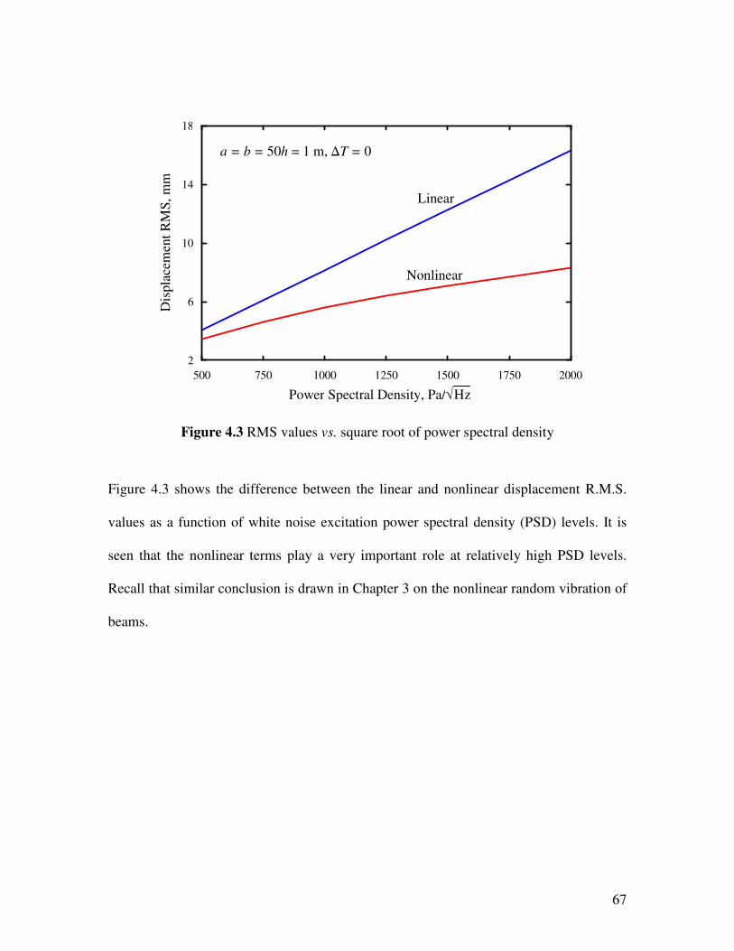
67

500 750 1000 1250 1500 1750 2000

Power Spectral Density, Pa/√Hz

2

6

10

14

18

Dis

pla

cem

ent

RM

S,

mm

Linear

Nonlinear

a = b = 50h = 1 m, DT = 0

Figure 4.3 RMS values vs. square root of power spectral density

Figure 4.3 shows the difference between the linear and nonlinear displacement R.M.S.

values as a function of white noise excitation power spectral density (PSD) levels. It is

seen that the nonlinear terms play a very important role at relatively high PSD levels.

Recall that similar conclusion is drawn in Chapter 3 on the nonlinear random vibration of

beams.

68

4.4 Temperature Effects on Random Vibrations of Composite

Plate

In this section the effect of temperature on the random vibration properties of composite

plate is examined. The existence of the temperature field exerts its influence on the

vibration characteristics of the composite plate by affecting the effective fundamental

frequencies of it.

The first order shear deformation plate theory (FSDT) (Reddy 2004) including the

temperature force resultant terms is expressed by Eqs. (4.33)-(4.37) in which the

superscripts “T” represent the temperature-introduced force or moment resultant terms.

2 2 2 2 2 2 2 2

11 12 662 2 2 2



∂ ∂ ∂ ∂ ∂ ∂ ∂ ∂ ∂ ∂ ∂ ∂+ + + + + + + ∂ ∂ ∂ ∂ ∂ ∂ ∂ ∂ ∂ ∂ ∂ ∂ ∂ ∂ ∂ ∂

2 2 2 2 2 2

11 12 66 0 12 2 2 2

TTxyxx

NN uB B B I I

x x y y y x x y t t

φ ψ φ ψ φ ∂ ∂∂ ∂ ∂ ∂ ∂ ∂+ + + + + + = + ∂ ∂ ∂ ∂ ∂ ∂ ∂ ∂ ∂ ∂

(4.33)

2 2 2 2 2 2 2 2

12 22 662 2 2 2



∂ ∂ ∂ ∂ ∂ ∂ ∂ ∂ ∂ ∂ ∂ ∂+ + + + + + + ∂ ∂ ∂ ∂ ∂ ∂ ∂ ∂ ∂ ∂ ∂ ∂ ∂ ∂ ∂ ∂

2 2 2 2 2 2

12 22 66 0 12 2 2 2

T T

xy yyN N vB B B I I

x y y x y x x y t t

φ ψ φ ψ ψ ∂ ∂ ∂ ∂ ∂ ∂ ∂ ∂+ + + + + + = + ∂ ∂ ∂ ∂ ∂ ∂ ∂ ∂ ∂ ∂

(4.34)

69

2 2 2 2 2 2

44 55 11 122 2 2 2

w w u w w v w wKA KA A A

y y x x x x x y x y y x

ψ φ ∂ ∂ ∂ ∂ ∂ ∂ ∂ ∂ ∂ ∂+ + + + + + + ∂ ∂ ∂ ∂ ∂ ∂ ∂ ∂ ∂ ∂ ∂ ∂

2 2 2 2 2 2 2 2

66 11 12 662 2 2 2

u v w w w w wA B B B

y x y x y y x y x x y y y x x

φ ψ φ ψ ∂ ∂ ∂ ∂ ∂ ∂ ∂ ∂ ∂ ∂ ∂+ + + + + + + + ∂ ∂ ∂ ∂ ∂ ∂ ∂ ∂ ∂ ∂ ∂ ∂ ∂ ∂ ∂

2 2 2 2 2 2 2 2

12 22 662 2 2 2



∂ ∂ ∂ ∂ ∂ ∂ ∂ ∂ ∂ ∂ ∂ ∂+ + + + + + + + ∂ ∂ ∂ ∂ ∂ ∂ ∂ ∂ ∂ ∂ ∂ ∂ ∂ ∂ ∂ ∂

2 2 2 2

12 22 66 112 2

1

2

w u w wB B B A

x y y x y x y x x x

φ ψ φ ψ ∂ ∂ ∂ ∂ ∂ ∂ ∂ ∂ + + + + + + ∂ ∂ ∂ ∂ ∂ ∂ ∂ ∂ ∂ ∂

2 2

12 11 66 662

12

2

v w w w u v w w wA B A B

y y y x x x y x y y x x y

φ φ ψ ∂ ∂ ∂ ∂ ∂ ∂ ∂ ∂ ∂ ∂ ∂ ∂+ + + + + + + + ∂ ∂ ∂ ∂ ∂ ∂ ∂ ∂ ∂ ∂ ∂ ∂ ∂

2

12 22 12 22 2

2

0 2

1 1( ) ( )

2 2

T T T T

xx xy xy yy

u w w v w w wA A B B

x x x y y y x y y

w w w w wN N N N q I

x x y y x y t

φ ψ ∂ ∂ ∂ ∂ ∂ ∂ ∂ ∂ ∂+ + + + + + ∂ ∂ ∂ ∂ ∂ ∂ ∂ ∂ ∂

∂ ∂ ∂ ∂ ∂ ∂ ∂+ + + + + = ∂ ∂ ∂ ∂ ∂ ∂ ∂

(4.35)

2 2 2 2 2 2 2 2

11 12 662 2 2 2


x x x x y y x y y y x y x y x y

∂ ∂ ∂ ∂ ∂ ∂ ∂ ∂ ∂ ∂ ∂ ∂+ + + + + + + ∂ ∂ ∂ ∂ ∂ ∂ ∂ ∂ ∂ ∂ ∂ ∂ ∂ ∂ ∂ ∂

2 2 2 2 2 2

11 12 66 55 2 12 2 2 2

w uD D D A I I

x y x y y x x t t

φ ψ φ ψ φκ φ

∂ ∂ ∂ ∂ ∂ ∂ ∂ + + + + − + = + ∂ ∂ ∂ ∂ ∂ ∂ ∂ ∂ ∂ (4.36)

2 2 2 2 2 2 2 2

12 22 662 2 2 2


x y x x y y y y x y x y x x x y

∂ ∂ ∂ ∂ ∂ ∂ ∂ ∂ ∂ ∂ ∂ ∂+ + + + + + + ∂ ∂ ∂ ∂ ∂ ∂ ∂ ∂ ∂ ∂ ∂ ∂ ∂ ∂ ∂ ∂

2 2 2 2 2 2

12 22 66 44 2 12 2 2 2

w vD D D A I I

x y y x y x y t t

φ ψ φ ψ ψκ ψ

∂ ∂ ∂ ∂ ∂ ∂ ∂+ + + + − + = + ∂ ∂ ∂ ∂ ∂ ∂ ∂ ∂ ∂

(4.37)

As an example, a special case is examined where the plate is subjected to a temperature

gradient varying in the thickness direction only. The composite plate has the same

70

material properties as listed in Section 4.3. The temperatures at the top surfaces is

increased to a certain value and the temperature at the bottom surface increased/decreased

to another value, which creates a steady-state heat transfer problem along the thickness

direction of the plate governed by the following equation within each layer

( )

( ) 0i

d dT zk z

dz dz

− = (4.38)

where ik is the thermal conductivity of the i-th layer of the composite plate.

The boundary conditions considered here are

tT T= at 2

hz =

bT T= at 2

hz −= (4.39)

and ( ) ( )1i iT z T z −= at each interface

where the subscript “b” and “t” refer to the top and bottom surface, respectively.

The thermal force resultants introduced by the varying temperature field can be obtained

from

1

11 12 16

12 22 26

1

16 26 66

( , , )

( , , )

( , , )

k

k

T

xx xxNz

T T

yy yyz

kT

xy xyk

N Q Q Q T x y z

N N Q Q Q T x y z dz

N Q Q Q T x y z

ααα

+

=

− ∆

= = − ∆ − ∆

∑∫ (4.40)

where ijα is the thermal expansion coefficient in the ij-th direction of the composite

plate, and ijQ s are defined in Appendix B.

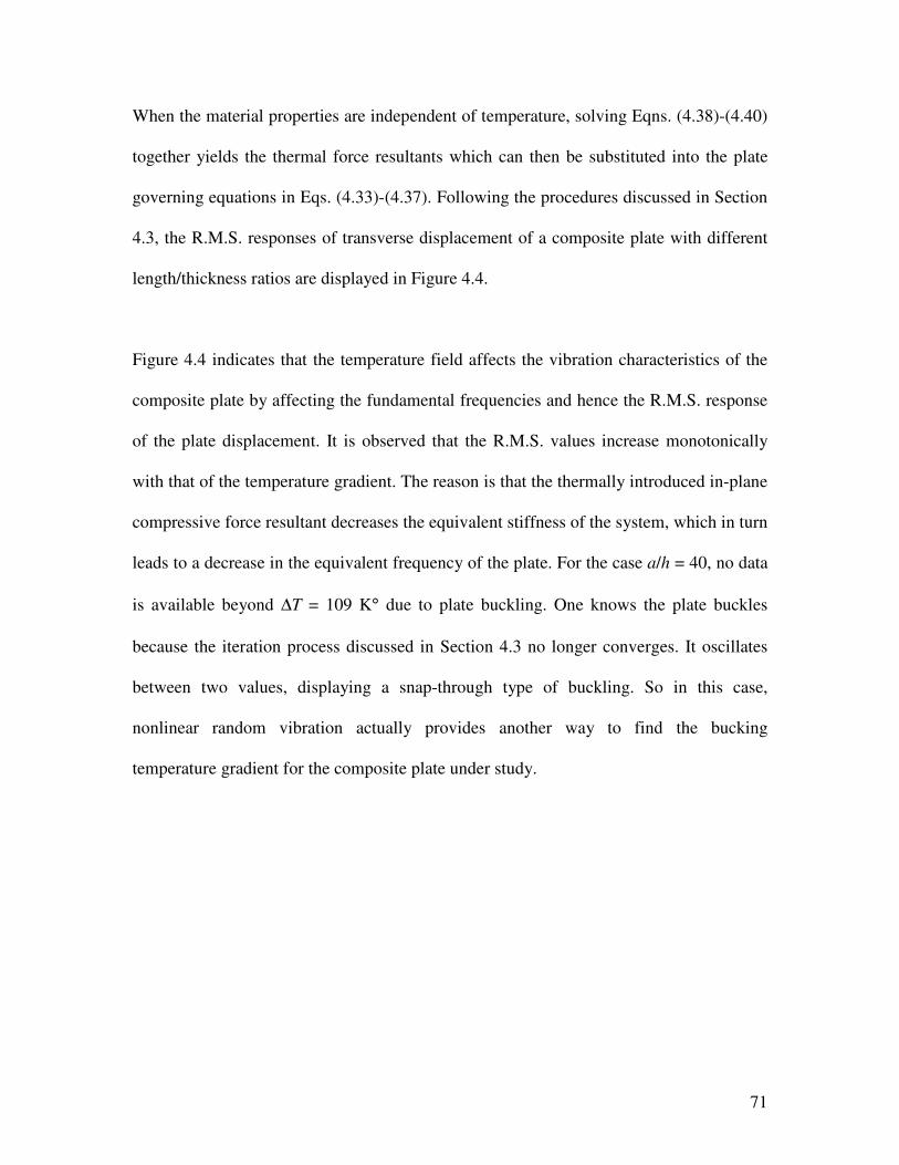
71

When the material properties are independent of temperature, solving Eqns. (4.38)-(4.40)

together yields the thermal force resultants which can then be substituted into the plate

governing equations in Eqs. (4.33)-(4.37). Following the procedures discussed in Section

4.3, the R.M.S. responses of transverse displacement of a composite plate with different

length/thickness ratios are displayed in Figure 4.4.

Figure 4.4 indicates that the temperature field affects the vibration characteristics of the

composite plate by affecting the fundamental frequencies and hence the R.M.S. response

of the plate displacement. It is observed that the R.M.S. values increase monotonically

with that of the temperature gradient. The reason is that the thermally introduced in-plane

compressive force resultant decreases the equivalent stiffness of the system, which in turn

leads to a decrease in the equivalent frequency of the plate. For the case a/h = 40, no data

is available beyond ∆T = 109 K° due to plate buckling. One knows the plate buckles

because the iteration process discussed in Section 4.3 no longer converges. It oscillates

between two values, displaying a snap-through type of buckling. So in this case,

nonlinear random vibration actually provides another way to find the bucking

temperature gradient for the composite plate under study.

72

0 50 100 150 200

Temperature Change DT, ∞K

1

3

5

7

9

Dis

pla

cem

ent

RM

S,

mm

a

h = 20

a

h = 30

a

h = 40

a = b = 1 mPlate Buckles

Figure 4.4 R.M.S. values vs. T (based on FSDT)

4.5 Comparison between FSDT and CPT

So far the first order shear deformation theory (FSDT) has been used throughout the

numerical examples. The key difference between the FSDT and classical plate theory

(CPT) is that the former takes into account the transverse shear strains. In other words,

the transverse normals are no longer perpendicular to the mid-plane of the plate after

deformation. In this section both theories are applied to study the R.M.S. response of the

same composite plate and the results are compared in Figure 4.5

73

In Figure 4.5 the calculated R.M.S. values under different temperature gradient (∆T) and

plate aspect ratios are shown. As the plate becomes thicker, the difference of the R.M.S.

responses based on the two theories becomes more significant. However, for relatively

high a/h ratios (> 40), the two theories yield almost the same results. Again, no data is

available beyond a/h = 32 for the FSDT case (∆T = 200 K°) due to plate buckling.

10 20 30 40 50

a/h

0.95

1.00

1.05

1.10

1.15

1.20

Dis

pla

cem

ent R

MS

Rat

io

a = b, h = 0.02 m

DT = 0 (FSDT)

DT = 200 ∞K (FSDT)

CPT

Plate Buckles

Figure 4.5 Variations of the ratios between FSDT and CPT R.M.S. values

vs. plate length to thickness ratio a/h

4.6 R.M.S. Stresses Calculation

So far in this chapter attention has been paid to the R.M.S. of displacement response.

Since the stress is a function of the displacement, the stochastic nature of the response

dictates that stress within the plate also varies with time. The R.M.S. values of stress

74

components are very useful numbers when it comes to the fatigue analysis of structures.

So in this section, the calculation of R.M.S. values of stress components at a given

location (x, y, z) within the plate is briefly discussed.

First, recall that the definitions of the nonlinear strains and stresses are:

2

2

1

2

1

2

0

0

xx

xxyy

yy

xyxy

yz

xz

u wT

x x

xv wT

y yy

u v w w zTy x x y

y xw

y

w

x

αφ

ε α ψε

γ α φ ψγ

γ ψ

φ

∂ ∂+ − ∆

∂ ∂ ∂

∂∂ ∂+ − ∆ ∂∂ ∂

∂∂ ∂ ∂ ∂= ++ + − ∆ ∂ ∂∂ ∂ ∂ ∂ +

∂ ∂∂

+∂

∂+

∂

(4.41)

11 12 16

21 22 26

16 26 66

xx xx

yy yy

xy xy

Q Q Q

Q Q Q

Q Q Q

σ εσ ετ γ

= (4.42)

Based on the above definitions, the value of E[ 2ijσ ] is not only function of the location

coordinate (x, y, z), but also E[ 2( )

mntU ], E[ 2

( )mn

tV ], E[ 2( )

mntW ], E[ 2

( )mn

tΦ ], and E[ 2( )

mntΨ ]

(note: under the assumption that both the load and response are zero-mean and follow

normal distribution, expectation of cross products of displacement components such as

E[ ( ) ( )mn mn

t tU V ], E[ ( ) ( )mn mn

t tΦ Ψ ], E[ 2( ) ( )

mn mnt tU W ], and E[ 2

( ) ( )mn mn

t tV W ] are zeroes.)

which are calculated from random vibration analysis. This is a straightforward but

tedious process due to the fact that so many terms are involved. But it can be efficiently

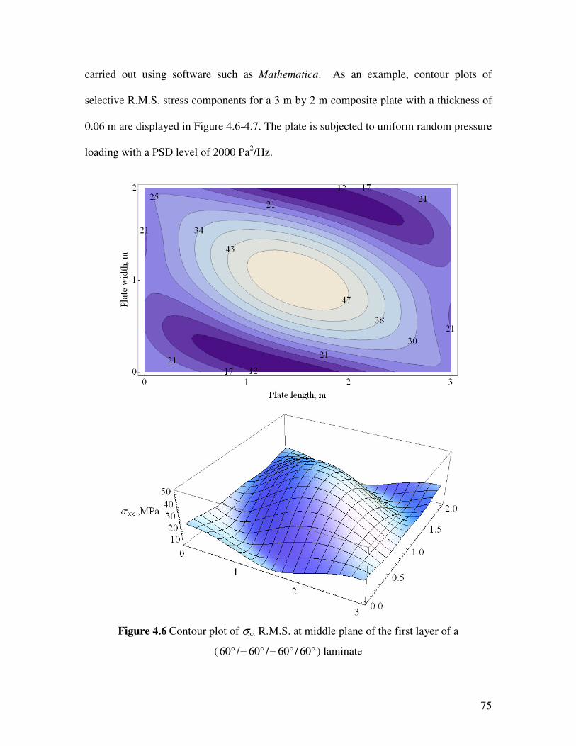
75

carried out using software such as Mathematica. As an example, contour plots of

selective R.M.S. stress components for a 3 m by 2 m composite plate with a thickness of

0.06 m are displayed in Figure 4.6-4.7. The plate is subjected to uniform random pressure

loading with a PSD level of 2000 Pa2/Hz.


( 60 / 60 / 60 / 60° − ° − ° ° ) laminate

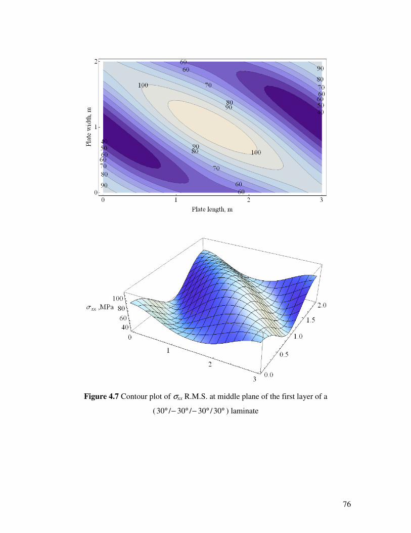
76


(30 / 30 / 30 /30° − ° − ° ° ) laminate

77

15 30 45 60 75

Ply angle θ, degree

σxx , -T = 0

σxx , -T = 200 Ko

σyy , -T = 0

σyy , -T = 200 Ko

τxy , -T = 0

τxy , -T = 200 Ko

0

100

200

300

400

Max

imu

m R

.M.S

. v

alu

e, M

Pa

Figure 4.8 Effect of ply angle θ on the maximal R.M.S. values of stress components

for a four-layer, 3m by 2m symmetric (θ/−θ/−θ/θ) laminate

In Figure 4.8, the effect of ply angle θ on the maximal R.M.S. values of stress

components for a four-layer symmetric (θ/−θ/−θ/θ ) laminate is displayed. The thickness

of the plate is 0.06 m. The plate is subjected to a random uniform pressure loading with a

PSD level of 2000 Pa2/Hz. It should be mentioned that no data is available for a

(15 / 15 / 15 /15° − ° − ° ° ) laminate subjected to a temperature gradient of 200 K° because

the plate would have buckled before that temperature increase is achieved. The results in

Figure 4.8 indicate that for this type of plate geometry, the ply angle has significant

influence on the R.M.S. value of a certain stress component. For this example, yy

σ is the

dominant stress component. On the other hand, the temperature gradient

top bottomT T T∆ = − has similar effect on the maximal R.M.S. of stresses as it does to the

78

transverse displacement response. That is, an increase in T∆ causes an increase in the

maximal value of the R.M.S. of stresses.

To summarize, in this chapter a systematical study of the random vibration of composite

plates is conducted. Classical and first order shear deformation plate theory are used and

compared. Similar to what the beam problem reveals, the nonlinear effect is very

significant as the level of loading spectral density increases. Temperature effects on both

the R.M.S. response of the transverse displacement and the maximum stress components

are studied.

79

Chapter 5. ARMA Model and Its Applications in

Random Vibration Data Analysis

5.1 Introduction

In Chapter 3 and Chapter 4 numerical simulations are performed under random

excitations whose PSDs (power spectral density) are already known or readily available.

However, in real life a certain random excitation’s PSD is usually not known and needs

to be obtained first in order to evaluate the dynamic response such as the R.M.S. of the

system. In other cases data of only limited length is available while data of extended

length is desired such as the strain input for random fatigue test. Such scenarios propel

one to come up with a numerical model based on limited amount of data at hand that can

then be used to represent the original data and extend it to any length in the time domain.

In doing that, the biggest concern is if the spectral features of the original data can still be

preserved during this modeling process. The statistical ARMA (autoregressive moving

average) model turns out to be a great tool in achieving the above goals. As will be

explained in the following chapter, ARMA model allows us the opportunity to generate

80

an analytical expression that simulates an infinite long random process. Also, the PSD

associated with the model can be explicitly expressed as a function of frequency and used

to represent the spectrum of the original data.

Some features make ARMA model very appealing in the applications of random

vibration analysis. First, it is very efficient in reconstructing the random signal. Second,

compared to other random simulation techniques such as Monte Carlo method, ARMA

model is very concise in its formulation, requiring very few parameters while preserving

the stochastic nature and spectral characteristics of the original signal. Third, it produces

simulation in the time domain directly instead of in the frequency domain.

5.2 Theoretical Background

By definition, an autoregressive moving average (ARMA) model of order (p, q) is written

as

1 1 2 2 1 1 2 2... ...t t t p t p t t t q t qx x x x x x xφ φ φ ε θ θ θ− − − − − −= + + + + − − − − (5.1)

where tε is a zero-mean Gaussian or Normal process and 1φ , …, pφ , 1θ ,…, qθ are

parameters associated with the model. The model is actually made of two parts, namely,

the autoregressive (AR) part in Eq.(5.2) and a moving average (MA) part as shown in

Eq.(5.3).

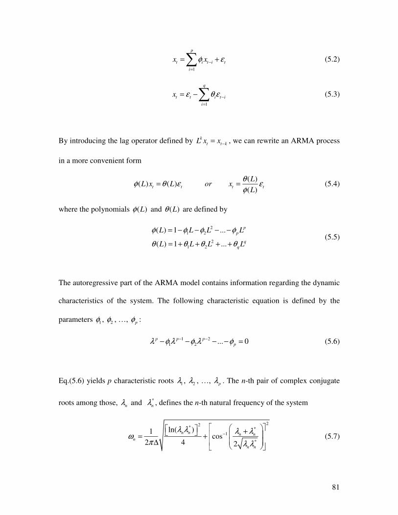
81

1

p

t i t i t

i

x xφ ε−

=

= +∑ (5.2)

1

q

t t i t i

i

x ε θ ε −

=

= −∑ (5.3)

By introducing the lag operator defined by k

t t kL x x −= , we can rewrite an ARMA process

in a more convenient form

( )

( ) ( )( )

t t t t

LL x L or x

L

θφ θ ε ε

φ= = (5.4)

where the polynomials ( )Lφ and ( )Lθ are defined by

2

1 2

2

1 2

( ) 1 ...

( ) 1 ...

p

p

q

q

L L L L

L L L L

φ φ φ φ

θ θ θ θ

= − − − −

= + + + + (5.5)

The autoregressive part of the ARMA model contains information regarding the dynamic

characteristics of the system. The following characteristic equation is defined by the

parameters 1φ , 2φ , …, pφ :

1 2

1 2 ... 0p p p

pλ φ λ φ λ φ− −− − − − = (5.6)

Eq.(5.6) yields p characteristic roots 1λ , 2λ , …, pλ . The n-th pair of complex conjugate

roots among those, nλ and *

nλ , defines the n-th natural frequency of the system

22* *

1

*

ln( )1cos

2 4 2

n n n nn

n n

λ λ λ λω

π λ λ−

+ = + ∆

(5.7)

82

where ∆ is the sampling interval.

After certain manipulations, Eq.(5.3) can be rewritten into the following form

0

t

t p t p

p

x G ε −

=

=∑ (5.8)

where by definition “ pG ”s are Green’s functions. From Eq.(5.8) it can be seen that the tx

can be represented as a linear combination of the disturbance acting on the system. The

value of pG indicates the influence of the previous tε at time interval p on the future

response of tx . For the ARMA(p, p -1) model, the elements of pG are determined as

follows

1 1 2 2 ...k k k

k p pG g g gλ λ λ= + + + (5.9)

where 1λ , 2λ , …, pλ are the roots of Eq.(5.6) and

1 2

1 1

1

1 1

( ... )

( ) ( )

p p

i i p

i pi

i k i k

k k i

gλ θ λ θ

λ λ λ λ

− −−

−

= = +

− − −=

− −∏ ∏ (5.10)

The variance of the model 0γ , 1γ , … pγ can be solved from a system of coupled p

equations:

2

1 1 0 1 1... ( ... ) 1, 2...,k k p k p k k q q k k pεγ φ γ φ γ σ θ ψ θ ψ θ ψ− − + −= + + − + + + = (5.11)

where jψ is defined recursively by the relationship

1 1 2 2 ...j j j p j p jψ ψ ψ ψ ψ ψ ψ θ− − −= + + + − (5.12)

with 0 1ψ = , and 0jθ = for j q> .

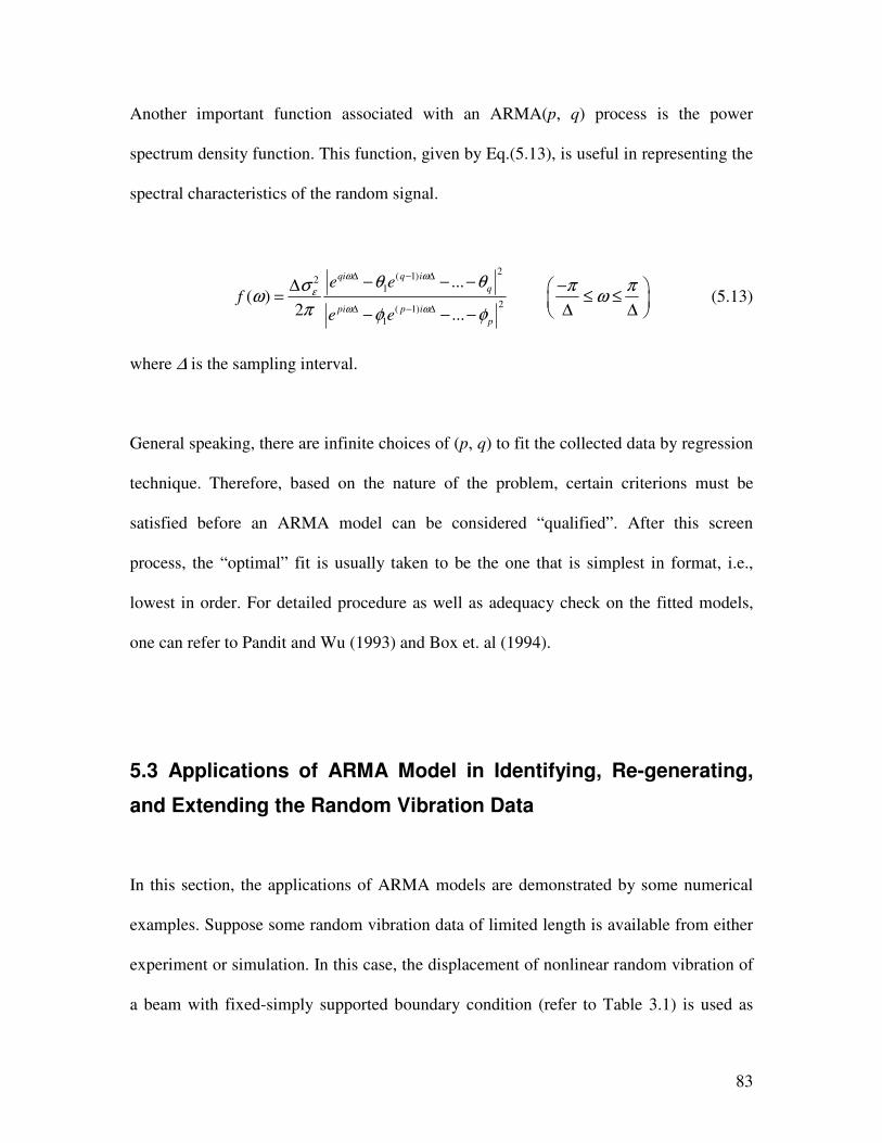
83

Another important function associated with an ARMA(p, q) process is the power

spectrum density function. This function, given by Eq.(5.13), is useful in representing the

spectral characteristics of the random signal.

2( 1)2

1

2( 1)

1

...( )

2 ...

qi q i

q

pi p i

p

e ef

e e

ω ω

ε

ω ω

θ θσ π πω ω

π φ φ

∆ − ∆

∆ − ∆

− − −∆ − = ≤ ≤ ∆ ∆ − − − (5.13)

where ∆ is the sampling interval.

General speaking, there are infinite choices of (p, q) to fit the collected data by regression

technique. Therefore, based on the nature of the problem, certain criterions must be

satisfied before an ARMA model can be considered “qualified”. After this screen

process, the “optimal” fit is usually taken to be the one that is simplest in format, i.e.,

lowest in order. For detailed procedure as well as adequacy check on the fitted models,

one can refer to Pandit and Wu (1993) and Box et. al (1994).

5.3 Applications of ARMA Model in Identifying, Re-generating,

and Extending the Random Vibration Data

In this section, the applications of ARMA models are demonstrated by some numerical

examples. Suppose some random vibration data of limited length is available from either

experiment or simulation. In this case, the displacement of nonlinear random vibration of

a beam with fixed-simply supported boundary condition (refer to Table 3.1) is used as

84

input. The beam is subjected to half uniform load. First, different orders of ARMA

models are fitted to the data and the harmonic components within the data are predicted

using Eq. (5.6) to (5.7). Second, once the ARMA(p, q) parameters 1φ , …, pφ , 1θ ,…, qθ

are obtained, Eq. (5.1) is used to re-generate the displacement response data and this set

of data is compared with the original signal. Third, since tε is the pure noise that follows

normal distribution, it can be generated via random normal number generator once the

variance is found in the previous steps. Substituting thus-obtained tε along with the

parameters 1φ , …, pφ , 1θ ,…, and qθ into Eq. (5.1), an analytical express is found that

can be used to generate time series of any desired length depending on the special needs

of the situation.

Selected ARMA(m, n) models are fitted to represent the simulated displacement response

of mode 1 of the beam. The scheme by Pandit and Wu (1993) is used to estimate the

parameters of selected ARMA(p , q) models. The results are listed in Table 5.1 and 5.2.

Figure 5.1 shows the corresponding PSD of the response of the simulation data. It is

observed in Figure 5.1 that the response has a dominant harmonic component at about

900 Hz.

Theoretically, the response of a second-order system could be fitted with a second order

ARMA(2, 1) or even AR(2) model. However, since the sampling interval is so small, the

correlations between adjacent data points must be taken into consideration, which may

require a higher order ARMA model. Another possibility is that there are additional

modes that are introduced into the system due to the stochastic nature of the excitation.

85

Table 5.1 Estimated ARMA parameters for different order models

ARMA

parameters

ARMA (p, q) model

(2,1) (3,2) (4,3)

φ1 1.608 1.465 1.241

φ2 -1.057 -0.946 -1.160

φ3 -0.0211 0.668

φ4 -0.692

θ1 -0.269 -0.527 -0.591

θ2 -0.254 -0.680

θ3 -0.310

Table 5.2 Frequencies predicted by selected ARMA models in Table 5.1

ARMA (p, q) model Predicted frequency, Hz

(2,1) 857

(3,2) 917

(4,3) 875

0 400 800 1200 1600 2000Frequency, Hz

0

10

20

30

40

mm

2/H

z

Figure 5.1 PSD of the mode 1 of the beam displacement simulation data

The data in Table 5.2 indicates that the selected ARMA models in Table 5.1 all give very

good predictions of the dominant harmonic frequency component embedded in the signal.

86

After the ARMA(p, q) parameters 1φ , …, pφ , 1θ ,…, qθ are obtained as shown in Table

5.1 and the variance of tε is found, Eq. (5.1) is used to re-generate a time series based on

the ARMA model. The re-generated data is compared with the original simulation results.

Although ARMA(2,1) model gives a pretty good prediction of the frequency component

embedded in the signal, a look at the re-generated displacement field by the model

reveals that the simulated displacement quickly blows out of proportion, thus suggesting

an instability in the system. This is part of the problem associated with ARMA

applications. The condition of stability (Box et. al 1994) for a certain ARMA model

requires that the norm of the each of the complex root determined by Eq.(5.6) is less than

one. For the ARMA(2,1) parameters listed in Table 5.1, the norm of the two complex

roots is 1.028 which is just over one. That causes the instability of the re-generated data.

Hence, a higher order model is needed in order to produce a stable time series.

0 1 2 3 4Time, sec

-0.15

0

0.15

Dis

pla

cem

ent,

m

Figure 5.2 Displacement from simulation of mode 2 of a F-SS beam

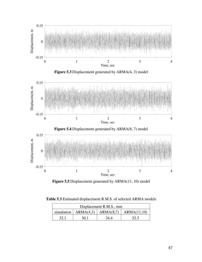
87

0 1 2 3 4Time, sec

-0.15

0

0.15

Dis

pla

cem

ent,

m

Figure 5.3 Displacement generated by ARMA(4, 3) model

0 1 2 3 4Time, sec

-0.15

0

0.15

Dis

pla

cem

ent,

m


0 1 2 3 4Time, sec

-0.15

0

0.15

Dis

pla

cem

ent,

m


Table 5.3 Estimated displacement R.M.S. of selected ARMA models

Displacement R.M.S., mm

simulation ARMA(4,3) ARMA(8,7) ARMA(11,10)

32.1 30.1 34.4 32.3

88

Further numerical examples are shown in Figures 5.2 to 5.5 for the mode 2 displacement

of the same beam. The original simulation result is shown in Figure 5.2. In this case

ARMA(3,2) model turns out to be unstable, so the lowest model used is ARMA(4, 3).

During the process, the estimated variance of the pure white noise part of each model is

used to produce random displacement data. That’s why the generated displacement looks

different each case. It is also seen that the generated displacement looks quite different

from the original data. In the original data, it is obvious that there is a significant

harmonic component. While in Figures 5.2 to 5.5, that harmonic component is shadowed

by the random noise. However, the R.M.S. of all the displacement data are very close, as

is shown in Table 5.3. So from the statistical point of view, they can be considered

“equivalent” signals. This is a very useful application of ARMA model because it can

extend data serial to unlimited length in the time domain while preserving the spectral

information of the original data. It is also observed that as the order of ARMA model

increases, the R.M.S. of the predicted displacement gets closer to that of the original

signal.

5.4 Comparison between PSD Curve from ARMA Model and

Newland’s Approach

There are some long-established methods that estimate the power spectral densities of

digital signals. One of the most widely used techniques was summarized by Newland

(1993). The detailed procedures are not repeated here. Although the guideline is the

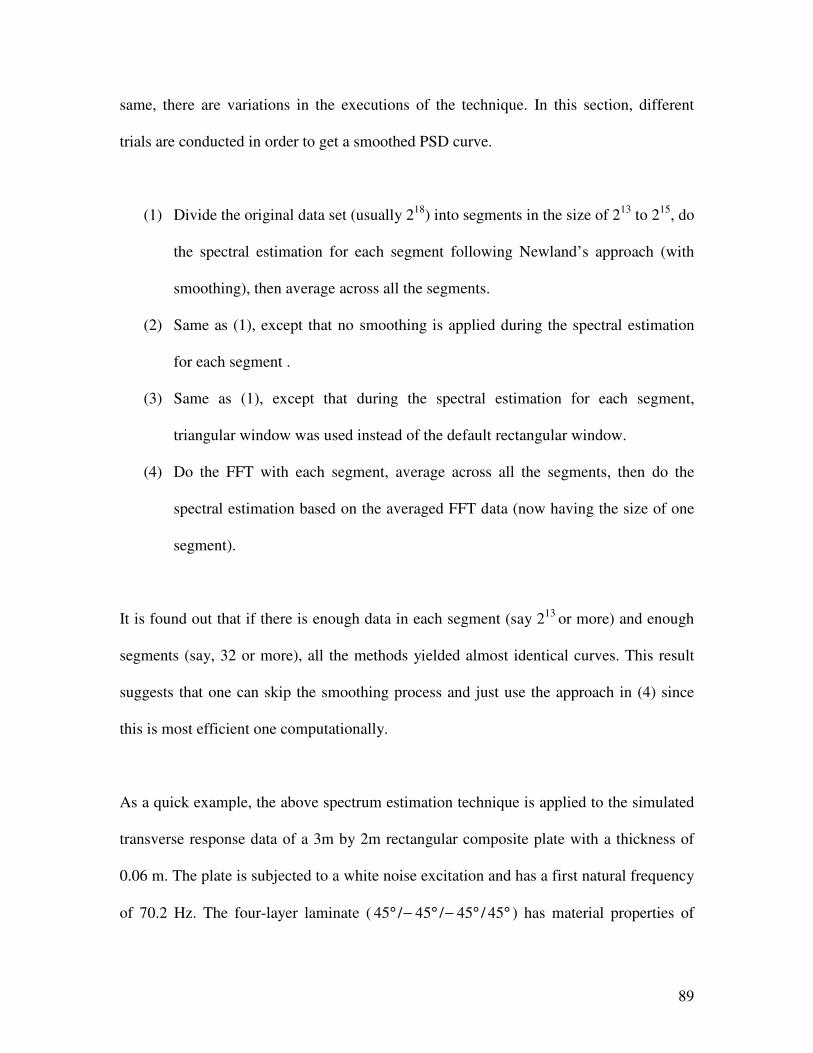
89

same, there are variations in the executions of the technique. In this section, different

trials are conducted in order to get a smoothed PSD curve.

(1) Divide the original data set (usually 218

) into segments in the size of 213

to 215

, do

the spectral estimation for each segment following Newland’s approach (with

smoothing), then average across all the segments.

(2) Same as (1), except that no smoothing is applied during the spectral estimation

for each segment .

(3) Same as (1), except that during the spectral estimation for each segment,

triangular window was used instead of the default rectangular window.

(4) Do the FFT with each segment, average across all the segments, then do the

spectral estimation based on the averaged FFT data (now having the size of one

segment).

It is found out that if there is enough data in each segment (say 213

or more) and enough

segments (say, 32 or more), all the methods yielded almost identical curves. This result

suggests that one can skip the smoothing process and just use the approach in (4) since

this is most efficient one computationally.

As a quick example, the above spectrum estimation technique is applied to the simulated

transverse response data of a 3m by 2m rectangular composite plate with a thickness of

0.06 m. The plate is subjected to a white noise excitation and has a first natural frequency

of 70.2 Hz. The four-layer laminate ( 45 / 45 / 45 / 45° − ° − ° ° ) has material properties of

90

3

1 2 3 1 12 13 12206.84 GPa, 0.1 , 10.34 GPa, 0.25, and 2070 kg/m .E E E E G G υ ρ= = = = = = =

The size of the simulation data is 218

which is divided into 32 sections. In Figure 5.6

selected 8 out of the 32 segments are displayed. The averaged PSD curve via Newland’s

approach is plotted in Figure 5.7.

The PSD plot given by Eq. (5.13) based on an ARMA(4,3) model is plotted in Figure 5.7

along with the estimated PSD curve from simulation data. Although the curves from the

two approaches don’t overlap, especially the height of the peaks, the areas under the

curves that represent the variance of the data are very close to each other, which is what

is expected. Generally Newland’s approach gives a very conservative estimation for the

PSD curve. It tends to underestimate the peak values.

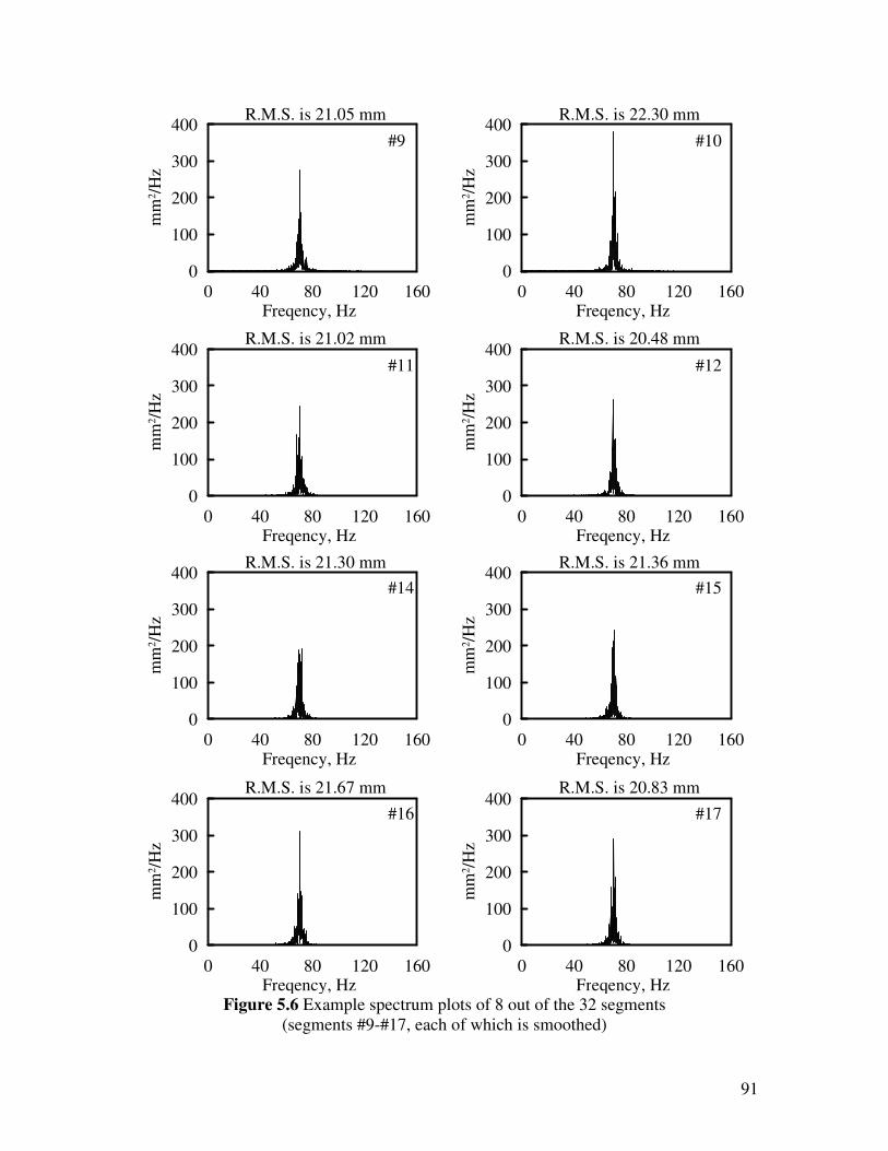
91

0 40 80 120 160Freqency, Hz

0

200

400

100

300m

m2/H

z

0 40 80 120 160Freqency, Hz

0

200

400

100

300

mm

2/H

z

0 40 80 120 160Freqency, Hz

0

200

400

100

300

mm

2/H

z

0 40 80 120 160Freqency, Hz

0

200

400

100

300

mm

2/H

z

0 40 80 120 160Freqency, Hz

0

200

400

100

300

mm

2/H

z

0 40 80 120 160Freqency, Hz

0

200

400

100

300

mm

2/H

z

0 40 80 120 160Freqency, Hz

0

200

400

100

300

mm

2/H

z

0 40 80 120 160Freqency, Hz

0

200

400

100

300

mm

2/H

z

R.M.S. is 22.30 mmR.M.S. is 21.05 mm

R.M.S. is 20.48 mmR.M.S. is 21.02 mm

R.M.S. is 21.36 mmR.M.S. is 21.30 mm

R.M.S. is 20.83 mmR.M.S. is 21.67 mm

#9 #10

#11 #12

#14 #15

#16 #17

Figure 5.6 Example spectrum plots of 8 out of the 32 segments

(segments #9-#17, each of which is smoothed)

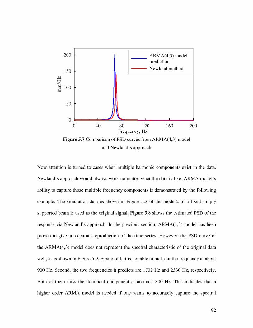
92

0 40 80 120 160 200Frequency, Hz

0

50

100

150

200m

m2/H

zARMA(4,3) model

prediction

Newland method

Figure 5.7 Comparison of PSD curves from ARMA(4,3) model

and Newland’s approach

Now attention is turned to cases when multiple harmonic components exist in the data.

Newland’s approach would always work no matter what the data is like. ARMA model’s

ability to capture those multiple frequency components is demonstrated by the following

example. The simulation data as shown in Figure 5.3 of the mode 2 of a fixed-simply

supported beam is used as the original signal. Figure 5.8 shows the estimated PSD of the

response via Newland’s approach. In the previous section, ARMA(4,3) model has been

proven to give an accurate reproduction of the time series. However, the PSD curve of

the ARMA(4,3) model does not represent the spectral characteristic of the original data

well, as is shown in Figure 5.9. First of all, it is not able to pick out the frequency at about

900 Hz. Second, the two frequencies it predicts are 1732 Hz and 2330 Hz, respectively.

Both of them miss the dominant component at around 1800 Hz. This indicates that a

higher order ARMA model is needed if one wants to accurately capture the spectral

93

properties of the signal. So in the next steps, ARMA(5,4), ARMA(6,5), …,

ARMA(11,10) models are tested. The details for the intermediate models are not shown

here. When ARMA(11,10) model is selected, it successfully picks out five harmonic

components: 918 Hz, 1733 Hz, 2023 Hz, 2626 Hz, and 3482 Hz. The PSD plot associated

with the ARMA(11,10) model is shown in Figure 5.11. By comparing the curves in

Figures 5.9 and 5.11, it can be found that the PSD curve via ARMA(11,10) model is

almost a perfect match to the one by Newland’s approach. Not only does it capture all the

spectral characteristics, but gives a smooth curve with an analytical expression as

compared to the sketchy one estimated from the Newland’s approach. Therefore, it can

be concluded that once the order of the ARMA model is high enough, it will accurately

predict the PSD of the signal.

0 1000 2000 3000 4000Frequency, Hz

0

1

2

3

4

mm

2/H

z

Figure 5.8 PSD of the beam simulation displacement data (Newland’s approach)

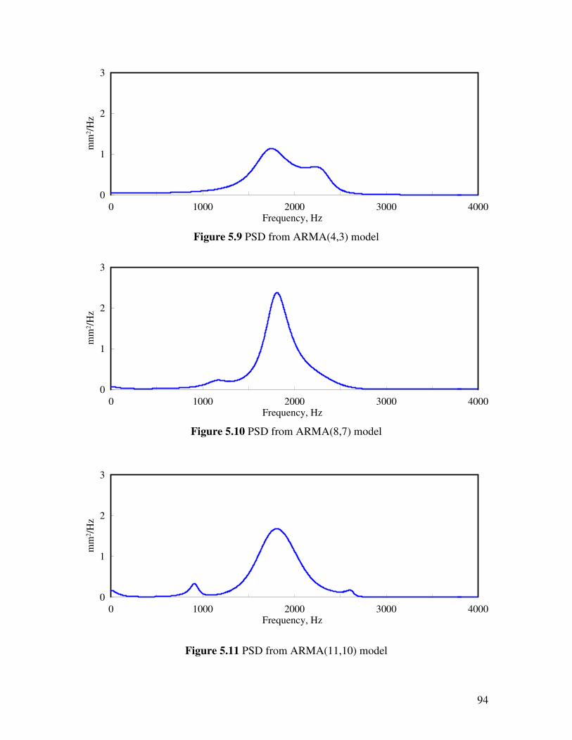
94

0 1000 2000 3000 4000Frequency, Hz

0

1

2

3

mm

2/H

z

Figure 5.9 PSD from ARMA(4,3) model

0 1000 2000 3000 4000Frequency, Hz

0

1

2

3

mm

2/H

z


0 1000 2000 3000 4000Frequency, Hz

0

1

2

3

mm

2/H

z


95

In summary, the ability of ARMA models in identifying, re-generating, and extending the

random vibration data is demonstrated and verified in this chapter. If one is only

interested in regenerating the displacement response and using it as a random input for

situations such as structural fatigue analysis, relatively lower ARMA models are efficient

enough to get the job done. However, higher order models are required to accurately

capture the spectral characteristics of the random signal. Overall, ARMA models have

great potentials in the analysis and application of random vibration data.

96

Chapter 6. Future Work

6.1 Durability of Structures Subjected to Random Loading

So far in this study the dynamic response of beams and plates under stochastic loading

conditions has been examined. One significant type of reliability concern associated with

oscillating loads of random nature is fatigue. As the magnitude and the direction of the

load vary incessantly with time, the material undergoes fluctuating strains that may

eventually cause the structure to fail at a stress well below the yield stress of the

constituent material. The most straightforward way to evaluate fatigue is the S-N curve.

The S-N curve is obtained through experiments in which a material under study is

subjected to a cyclic stress and the number of cycles to failure is counted. Numerous tests

are run at different stress levels and a smooth curve is drawn with the help of some

knowledge of data processing or linear regression technique. Traditional theories in

fatigue include Miner’s Rule and Paris’ equation. Miner (1945) proposed that failure

occurs if the following relationship for a material subjected to k different stress levels is

satisfied

97

1

k

i

ii

nC

N=

=∑ (6.1)

where C is a constant determined experimentally and ranges from 0.7 to 2.2, and in

represents the number of cycles under the i-th stress level and iN is the total number of

cycles before failure.

The expected fatigue damage after duration of time T under random loading is found to

be (Liou et al. 1999)

[ ] 00

( )( )

( )

d

f m

pE D T v T d

N

σ σσ

σ σ

∞+

= ∫ (6.2)

where [ ]E • means the mathematical expectation, d is Morrow’s plastic work interaction

exponent, 0v+ represents the number of stress cycle per unit time for a narrow-band

process, ( )p σ is the PDF (probability density function) of stress amplitudes, mσ is the

maximum stress magnitude, and ( )fN σ is the number of stress peaks to cause failure if a

constant amplitude σ is applied and can be obtained from the Basquin’s equation:

'p

fN Cσ = (6.3)

where p and 'C are material-dependant constants.

In Nigam and Narayanan (1994), the estimated fatigue damage after time T under

stationary narrow-band random vibration is expressed by

(0)

[ ( )] ( 2 ) 12

bb

q

x

N T qE D T

cσ

+ = Γ +

(6.4)

98

where 1

(0)2

x

x

Nσ

π σ+ = , [ ]Γ • represents the Gamma function, and c, q, b are constants

that depend on the material and shape of the specimen.

Furthermore, the PDF ( )p σ in Eq.(6.2) is expressed as

2

2 2( ) exp , 0

2rms rms

Pσ σ

σ σσ σ

= − >

(6.5)

where rmsσ is the R.M.S. or the standard deviation of the random stress process.

The above Eqs. (6.1)-(6.3) can be used to predict the fatigue damage of a component. To

be more specific, the constants p and C come from the material's S-N curve, and 0v+ , rmsσ

are determined by the given random loading. On the other hand, by setting the left side of

Eq.(6.2) to 1 and solving for T, one can obtain the fatigue life of the material.

Another approach to look at the reliability issue is to examine the probability of

displacement W(t) exceeding a specific value η within a specified time interval. Lin

(1967) and Nigam (1983) defined the following reliability function for a stationary

random process

[ ]( , ) exp ( )R t v tη η= − (6.6)

and the function ( )v η is defined by

2 2

2

1( ) exp

2 2

w

w w

vσ η

ηπ σ σ

= −

(6.7)

where wσ is the R.M.S. of the transverse velocity. In similar fashion as what is done in

Chapter 3 to calculate the R.M.S. of W(t), one has (while neglecting the cross-correlation

terms in the case of small damping)

99

2 2 2 2

,

( , ) ( ) ( )mn mnw mn Q Q

m n

W x y S H dσ ω ω ω ω∞

−∞=∑ ∫

(6.8)

where (m, n) represents mode number.

Using Eqs. (6.6)-(6.8), the reliability vs. time curve can be obtained for a beam or plate

subjected to a known random excitation. Due to the fact that this is a straightforward

procedure and no material fatigue data is available, no numerical example is given while

the outline of the solution process is summarized here.

6.2 Future Work

The fatigue life analysis mentioned in section 6.1 is one area future work can be devoted.

So far this study has focused on the stationary random process whose statistical

properties do not vary with time. In reality many random excitations are non-stationary

such as earthquake wave. It would be interesting to examine the dynamic response of

structure as time evolves subjected to this type of loading condition. Different approaches

to model the non-stationary process can be found in work of Cederbaum et. al (1992).

On the other hand, although a new linearly coupled linearization method is proposed in

addition to the traditional equivalent linearization to obtain the numerical results in this

study, the limitation of this type of technique is that the load and system response must be

Gaussian. It has been discussed that technically when governing equations of motion of

100

the system are nonlinear, the responses can be non-Gaussian even if the loading is.

Hence, in order to pursue more accurate results for multi-degree systems, other

linearization techniques need to be explored for the higher-order beams or plates such as

the Gaussian closure technique, statistical linearization, and statistical non-linearization.

These are all potential fields where future can be conducted.

101

Reference

Abdelnaser, A.S. and Singh, M.P. (1993) Random response of antisymmetric angle-ply

composite plates with Levy boundary-conditions, Composite Engineering, 3(9),

817–833

Bao, G. and Wang, L. (1995) Multiple cracking in functionally graded ceramic/metal

coatings, International Journal of Solids and Structures, 32, 2853–2871

Birman, V (1995) Buckling of Functionally Graded Hybrid Composite Plates,

Proceeding of the 10th Conference on Engineering Mechanics, vol. 2, 1199–2202

Bolotin, V.V. (1984) Random vibrations of elastic systems. The Hague, The Netherlands:

Martinus Nijhoff

Boukhrist, A., Mourot, G. and Ragot, J. (1999) Non-linear dynamic system

identification: a multi-model approach, International Journal of Control, 72(7),

591–604

Box, G.E.P., Jenkins, G.M. and Reinsel, G.C. (1994) Time Series Analysis: Forecasting

and Control, 3rd

edition, Prentice-Hall, Inc.

Cai, H. and Bao, G. (1998) Crack bridging in functionally graded coatings. International

Journal of Solids and Structures, 35, 701–717

Carden, E.P. and Brownjohn, J.M.W. (2008) ARMA modelled time-series classification

for structural health monitoring of civil infrastructure, Mechanical Systems and

Signal Processing, 22, 295–314

Caughey, T.K. (1959a) Response of a non-linear string to random loading, Journal of

applied Mechanics, ASME, 26,341-344

Caughey, T.K. (1959b) Response of van der Pol oscillator to random excitation, Journal

of applied Mechanics, ASME, 26,345-348

102

Caughey, T. K., Equivalent Linearization Techniques (1963) Journal of Acoustic Society

of America, 35, 1706-1711

Cederbaum, G., Librescu, L. and Elishakoff, I. (1988) Random vibration of laminated

plates modeled within a high-order shear deformation theory, Journal of the

Acoustical Society of America, 84(2), 660-666

Cederbaum, G., Librescu, L. and Elishakoff, I. (1989) Remarks on a dynamic higher-

order theory of laminated plates and its application in random vibration,

International Journal of Solids and Structures, 25(5), 515–526

Chatfield, C. (1989) The Analysis of Time Series: An Introduction, Fourth Edition,

Chapman & Hall

Chen, C.S. (2005) Nonlinear vibration of a shear deformable functionally graded plate,

Composite Structures, 68, 295-302

Chen, Q. and Tomlison G.R. (1996) Parametric identification of systems with dry friction

and nonlinear stiffness using a time series model, Journal of Vibration and

Acoustics, 118 (2), 252–263

Chen, W.Q. and Ding, H.J. (2002) On free vibration of a functionally graded

piezoelectric rectangular plate, Acta Mechanica, 153 (3–4), 207–216

Cheng, Z.Q. and Batra, R.C. (2000a) Deflection relationships between the homogeneous

Kirchhoff plate theory and different functionally graded plate theories, Acta

Mechanica, 52, 143–158

Cheng, Z.Q. and Batra, R.C. (2000b) Exact correspondence between eigenvalues of

membranes and functionally graded simply supported polygonal plates, Journal of

Sound and Vibration, 229, 879–895

Cheng, Z.Q. and Batra, R.C. (2000c) Three-dimensional thermoelastic deformations of a

functionally graded elliptic plate, Composites: Part B, 31, 97–106

Chi, S.H., Chung, Y.L., 2002. Cracking in sigmoid functionally graded coating, Journal

of Mechanics, 18, 41–53

Chi, S.H., Chung, Y.L., (2003) Cracking in coating-substrate composites of multi-layered

and sigmoid FGM coatings, Engineering Fracture Mechanics, 70, 1227–1243

Chi, S.H., Chung, Y.L., (2006a) Mechanical behavior of functionally graded material

103

plates under transverse load—Part I: Analysis, International Journal of Solids and

Structures, 43(13), Pages 3657-3674

Chi, S.H., Chung, Y.L., (2006b) Mechanical behavior of functionally graded material

plates under transverse load—Part II: Numerical results, International Journal of

Solids and Structures, 43(13), Pages 3675-3691

Cho, J.R. and Oden, J.T. (2000) Functionally graded material: a parametric study on

thermal-stress characteristics using theCrank–Nicolson–Galerkin scheme,

Computer Methods in Applied Mechanics and Engineering, 188, 17–38

Chung, Y.L., Chi, S.H. (2001) The residual stress of functionally graded materials,

Journal of the Chinese Institute of Civil and Hydraulic Engineering, 13, 1–9

Chonan, S. (1995) Random vibration of a prestressed, orthotropic, thick rectangular plate

on a generalized flexible foundation, Journal of the Acoustical Society of America,

78(2), 598–604

Crandall, S.H. (1963) Perturbation techniques for random vibration of nonlinear systems,

Journal of Acoustical Society of America, 35, 1700-1705

Crandall, S.H., and Mark, W.D. (1973) Random vibration in mechanical systems, New

York: Academic Press

David, J.Y., Jones, S.A., and Giddens, D.P. (1991) Modern spectral analysis techniques

for blood flow velocity and spectral measurements with pulsed Doppler ultrasound,

IEEE Transactions on Biomedical Engineering, 38(6), 589–596

Dahlberg, T. (1999) The effect of modal coupling in random vibration analysis, Journal

of Sound and Vibration, 228(1), 157-176

Delale, F., and Erdogan, F. (1983) The crack problem for a nonhomogeneous plane,

ASME Journal of Applied Mechanics, 50, 609–614

Drake, J.T., Williamson, R.L., Rabin, B.H., (1993) Finite element analysis of thermal

residual stresses at graded ceramic–metal interfaces, Part II: interface optimization

for residual stress reduction, Journal of Applied Physics, 74, 1321–1326

Elishakoff, P. (1983) Probabilistic methods in the Theory of Structures, Wiley-

Interscience, New York

104

Elishakoff, I., Fang, J. and Caimi, R. (1995) Random vibration of a nonlinearly deformed

beam by a new stochastic linearization technique, International Journal of Solids

and Structures, 32(11), 1571–1584

Elishakoff, I. (1991). Method of stochastic linearization revised and improved, In

Computational Stochastic Mechanics (Edited by P. D. Spanos and C. A. Brebbia),

pp. 101-I 11. Computational Mechanics Publications and Elsevier Applied Science,

London.

Elishakoff, I. and Livshits, D. (1984). Some closed-form solutions in random vibration of

Bernoulli-Euler beams, International Journal of Engineering Science, 22, 1291-

1302

Elishakoff, I. and Zhang, R. C. (1991) Comparison of the new energy-based versions of

the stochastic linearization technique, In Nonlinear Stochastic Mechanics (Edited

by N. Bellomo and F. Casciati), pp. 201-212. Springer, Berlin.

Elmajid, A., Taya, M. and Hudnut, S. (2001) Analysis of out-of-plane displacement and

stress field in a piezocomposite plate with functionally graded microstructure,

International Journal of Solids and Structures, 38(19), 3377–3391

Er, G.K. (1998) Multi-Gaussian closure method for randomly excited nonlinear systems,

International Journal of Non-Linear Mechanics, 33(2), 201-214

Erdogan, F., Chen, Y.F. (1998) Interfacial cracking of FGM/metal bonds. In: Kokini, K.

(Ed.), Ceramic Coating, pp. 29–37

Erdogan, F., Wu, B.H. (1996) Crack problems in FGM layers under thermal stresses,

Journal of Thermal Stresses, 19, 237–265

Eringen, A. C. (1957). Response of beams and plates to random loads, Journal of Applied

Mechanics, 24, 46-52

Fang, J., Elishakoff, I. and Caimi, R. (1995) Nonlinear response of a beam under

stationary random excitation by improved stochastic linearization method, Applied

Mathematical Modelling, 19(2), 106-111

Feldman, E., Aboudi, J. (1997) Buckling analysis of functionally graded plates subjected

to uniaxial loading, Composite Structures, 38, 29–36

Foda, M.A., 1999. Influence of shear deformation and rotary inertia on nonlinear free

vibration of a beam with pinned ends, Computers and Structures, 71, 663–670

105

Ganapathi, M. and Prakash, T. (2006) Thermal buckling of simply supported functionally

graded skew plates, Composite Structures, 74(2), 247–250

Gardiner, C.W. (2004) Handbook of Stochastic Methods: for Physics, Chemistry and the

Natural Sciences (Springer Series in Synergetics), 3rd

edition, Springer

Gautier, P.E., Gontier, C., and Smail, M. (1995) Robustness of an ARMA identification

method for modal analysis of mechanical systems in the presence of noise, Journal

of Sound and Vibration, 179(2), 227-242

Gray, C.E., Decha-Umphait K. and Mei, C. (1985) Large Deflection, Large Amplitude

Vibrations and Random Response of Symmetrically Laminated Plates, Journal of

Aircraft, 22(11), 929-930

Gu, P., Asaro, R.J., 1997. Crack deflection in functionally graded materials, International


Guler, N.F., Kiymik, M.K., and Guler, I. (1995) Comparison of FFT and AR-based

sonogram outputs of 20 MHz pulsed Doppler data in real time, Computers in

Biology and Medicine, 25(4), 383–391

Guler, I., Kara, S., Guler, N.F., and Kiymik, M.K. (1996) Application of autoregressive

and fast Fourier transform spectral analysis to tricuspid and mitral valve stenosis,

Computer Methods and Programs in Biomedicine, 49, 29–36

Harichandran, R.S. and Naja, M.K. (1997) Random vibration of laminated composite

plates with material non-linearity, International Journal of Non-Linear Mechanics,

32(4), 707–720

He, X.Q., Ng, T.Y., Sivashanker, S., Liew, K.M., 2001. Active control of FGM plates

with integrated piezoelectric sensors and actuators, International Journal of Solids

and Structures, 38, 1641–1655

He, X.Q., Liew, K.M., Ng, T.Y. and Sivashanker, S. (2002) A FEM model for the active

control of curved FGM shells using piezoelectric sensor/actuator layers,

International Journal for Numerical Methods in Engineering, 54(6), 853–870

Herbert, R. E. (1964) Random vibrations of a nonlinear elastic beam, Journal of

Acoustical Society of America, 36, 2090-2094

Herbert, R. E. (1965) On the stresses in a nonlinear beam subject to random excitation,

International Journal of Solids and Structures, 1, 235-242

106

Huang, X.L. and Shen, H.S. (2004) Nonlinear vibration and dynamic response of

functionally graded plates in thermal environments, International Journal of Solids


Ibrahim, R.A. (1987) Structural dynamics with parameter uncertainties, Applied

Mechanics Review, 40(3) (1987) 309–328

Ichikawa, K. (2000) Functional Graded Materials in the 21st Century, Kluwer Academic

Publishers, Norwell, MA

Iyengar, R.N. and Dash, P.K. (1978) Study of the random vibration of non-linear systems

by the Gaussian closure technique, Journal of Applied Mechanics, ASME, 45, 393-

399

Jaksic, N. and Boltezar, M. (2002) An approach to parameter identification for a single-

degree-of-freedom dynamical system based on short free acceleration response,

Journal of Sound and Vibration, 250(3), 465–483

Javaheri, R.and Eslami, M. R. (2002) Buckling of Functionally Graded Plates under In-

plane Compressive Loading, ZAMM, 82(4), 277––283

Javaheri, R. and Eslami, M.R. (2002b) Thermal buckling of functionally graded plates.

AIAA Journal, 40(1), 162–169

Javaheri, R. and Eslami, M.R. (2002c) Thermal buckling of functionally graded plates

based on higher order theory, Journal of Thermal Stresses, 25, 603–625

Jin, Z.H., Batra, R.C., 1996. Stresses intensity relaxation at the tip of an edge crack in a

functionally graded material subjected to a thermal shock, Journal of Thermal

Stresses, 19, 317–339

Jin, Z.H., Noda, N., 1994. Crack tip singular fields in nonhomogeneous materials, ASME

Journal of Applied Mechanics, 61, 738–740

Jin, Z.H., Paulino, G.H., 2001. Transient thermal stress analysis of an edge crack in a

functionally graded material, International Journal of Fracture, 107, 73–98

Kaluzynski, K. (1987) Analysis of application possibilities of autoregressive modeling to

Doppler blood flow signal spectral analysis, Medical and Biological Engineering

and Computing, 25, 373–376

107

Kang, J., and Harichandran, R.S. (1999) Random vibration of laminated FRP plates with

material nonlinerity using high-order shear theory, Journal of Engineering

Mechanics, 9, 1081-1088

Kaysser W.A., and Ilschner, B. (1995) FGM research activities in Europe, MRS Bulletin,

20(1), 22–26

Kim, K.S., Noda, N. (2002) A Green’s function approach to the deflection of a FGM

plate under transient thermal loading, Archive of Applied Mechanics, 72, 127–137

Kitipornchai, S., Yang, J., and Liew, K.M. (2004) Semi-analytical solution for nonlinear

vibration of laminated FGM plates with geometric imperfections, International


Kitipornchai, S., Yang, J. and Liew, K.M. (2006) Random vibration of the functionally

graded laminates in thermal environments, Computer Methods in Applied

Mechanics and Engineering, 195 (2006) 1075–1095

Koizumi, M. (1997) FGM activities in Japan, Composites-Part B, 28(1/2), 1–4

Koizumi M, and Niino, M (1995) Overview of FGM research in Japan, MRS Bulletin,

20(1),19–21

Koizumi M. (1993) The concept of FGM, Ceramic Transactions, Functionally Gradient

Materials, 34, 3–10

Lanhe, W. (2004) Thermal buckling of a simply-supported moderately thick rectangular

FGM plate, Composite Structures, 64, 211–218

Lee, Y.D. and Erdogan, F. (1995) Residual/thermal stress in FGM and laminated thermal

barrier coatings, International Journal of Fracture, 69, 145–165

Liew, K.M., He, X.Q., Ng, T.Y., and Sivashanker, S. (2001) Active control of FGM

plates subjected to a temperature gradient: modeling via finite element method

based on FSDT, International Journal for Numerical Methods in Engineering, 52,

1253–1271

Liew, K.M., He, X.Q., Ng, T.Y. and Kitipornchai, S. (2002) Active control of FGM

shells subjected to a temperature gradient via piezoelectric sensor/actuator patches,

International Journal for Numerical Methods in Engineering, 55(6), 653–668

108

Liew, K.M., Lim, H.K., Tan, M.J. and He, X.Q. (2002) Analysis of laminated composite

beams and plates with piezoelectric patches using the element-free Galerkin

method, Computational Mechanics, 29(6), 486–497

Liew, K.M., He, X.Q. and Kitipornchai, S. (2004) Finite element method for the feedback

control of FGM shells in the frequency domain via piezoelectric sensors and

actuators, Computer Methods in Applied Mechanics and Engineering, 193(3–5),

257–273

Liew, K.M., Yang, J., and Kitipornchari, S. (2003) Postbuckling of piezoelectric FGM

plates subject to thermo-electromechanical loading, International Journal of Solids


Liew, K.M., Yang, J. and Kitipornchai, S. (2004) Thermal post-buckling of laminated

plates comprising functionally graded materials with temperature-dependent

properties, Journal of Applied Mechanics, 71(6), 839–850

Liew, K.M, He, X.Q. and Kitipornchai, S. (2004) Finite element method for the feedback

control of FGM shells in the frequency domain via piezoelectric sensors and

actuators, Computer Methods in Applied Mechanics and Engineering, 193(3–5),

257–273

Liew, K.M.， Yang， J. and Wu, Y.F. (2006) Nonlinear vibration of a coating-FGM-

substrate cylindrical panel subjected to a temperature gradient, Methods in Applied

Mechanics and Engineering, 195(9-12), 1007-1026

Lim, C.W. and He, L.H. (2001) Exact solution of a compositionally graded piezoelectric

layer under uniform stretch, bending and twisting, International Journal of

Mechanical Science, 43(11), 2479–2492

Lin, Y.K. (1973) Probabilistic theory of structural dynamics, New York: McGraw-Hill

Lin, Y.K. (1976) Probabilistic theory of structural dynamics, Malabar, FL: R.E. Krieger;

Loy, C.T., Lam, K.Y. and Reddy, J.N. (1999) Vibration of functionally graded cylindrical

shells, International Journal of Mechanical Science, 41, 309–324

Manohar, C.S. and Ibrahim, R.A. (1999) Progress in structural dynamics with stochastic

parameter variations: 1987–1998, Applied Mechanics Review, 52(5), 177–196

109

Mattson, S.G. and Pandit, S.M. (2006) Statistical moments of autoregressive model

residuals for damage localization, Mechanical Systems and Signal Processing,

20(3), 627–645

Mills, T.C. (1990) Time Series Techniques for Economists, Cambridge University Press

Miner, M.A. (1945) Cumulative damage in fatigue, Journal of Applied Mechanics, 12,

159–164

Mobarakeh, A.A., Rofooei, F.R., and Ahmadi, G. (2002) Simulation of earthquake

records using time-varying ARMA(2,1) model, Probabilistic Engineering

Mecahnics, 17, 15-34

Najafizadeh, M.M. and Eslami, M.R. (2002a) Buckling analysis of circular plates of

functionally graded materials under uniform radial compression, International

Journal of Mechanical Science, 44, 2479–2493

Najafizadeh M.M. and Eslami, M.R. (2002b) First-order-theory-based thermoelastic

stability of functionally graded material circular plates, AIAA Journal, 40(7), 1444–

1450

Najafizadeh, M.M., Eslami, M.R., 2002b. Thermoelastic stability of circular plates

composed of functionally graded materials under uniform radial compression.

International Journal of Mechanical Science, 44, 2479–2493

Na, K., and Kim, J. (2004) Three dimensional thermal buckling analysis of functionally

graded materials, Composites, Part B: Engineering, 35 (5), 429–437

Nayfeh, A. (1993) Introduction to Perturbation Techniques, Wiley-Interscience

Nayfeh, A. and Mook, D. (1995) Nonlinear Oscillations, Wiley-Interscience

Newland, D.E. (1993) An Introduction to random vibration, spectral and wavelet

analysis, London: Longman, third edition.

Ng, T.Y., Lam, Y.K., Liew, K.M., and Reddy, J.N. (2001). Dynamic stability analysis of

functionally graded cylindrical shell under periodic axial loading, International


Ng, T.Y., He, X.Q., and Liew, K.M. (2002) Finite element modeling of active control of

functionally graded shells in frequency domain via piezoelectric sensors and

actuators, Computational Mechanics, 28(1), 1–9

110

Nigam, N.C. (1983) Introduction to Random vibrations, Cambridge, Massachusetts: MIT

Press

Ootao, Y. and Tanigawa, Y. (2000) Three-dimensional transient piezothermoelasticity in

functionally graded rectangular plate bonded to a piezoelectric plate, International

Journal of Solids and Structures, 37(32), 4377–4401

Pandit, S.M. and Wu, S. (1993) Time series and system analysis with applications,

Malabar, Fla.: Krieger Pub. Co.

Park, J.S. and Kim, J.H. (2005) Thermal postbuckling and vibration analyses of

functionally graded plates, Journal of Sound and Vibration, 289(1-2), 77-93

Patel, B.P., Gupta, S.S., Loknath, M.S. and Kadu, C.P. (2005) Free vibration analysis of

functionally graded elliptical cylindrical shells using higher-order theory,

Composite Structures, 69(3), 259–270

Popescu, T.D., and Demetriu, S. (1990) Analysis and Simulation of Strong Earthquake

Ground Motions Using ARMA Models, Automatica, 26(4), 721-737

Pradhan, S.C., Loy, C.T., Lam, K.Y. and Reddy, J.N. (2000) Vibration characteristics of

functionally graded cylindrical shells under various boundary conditions, Applied

Acoustics, 61, 111–129

Praveen, G.N. and Reddy, J.N. (1998) Nonlinear transient thermoelastic analysis of

functionally graded ceramic–metal plates, International Journal of Solids and

Structures, 35, 4457–4476

Reddy, J.N. (1997) Mechanics of laminated composite plates: theory and analysis, Boca

Raton: CRC Press

Reddy, J.N. and Chin, C.D. (1998) Thermomechanical analysis of functionally graded

cylinders and plates, Journal of Thermal Stresses, 21, 593–626

Reddy, J.N. (2000) Analysis of functionally graded plates, International Journal for

Numerical Methods in Engineering, 47, 663–684

Reddy, J.N. and Cheng, Z.Q. (2001) Three-dimensional solutions of smart functionally

graded plates, Journal of Applied Mechanics, 68(2), 234–241

Reddy, J.N. and Cheng, Z.Q. (2002) Frequency correspondence between membranes and

functionally graded spherical shallow shells of polygonal platform, International

Journal of Mechanical Sciences, 44(5), 967–985

111

Reddy, J.N. (2004) Mechanics of laminated composite plates and shells: theory and

analysis, second edition, Boca Raton: CRC Press

Reiter, T. and Dvorak, G.J. and Tvergaard, V. (1997) Micromechanical models for

graded composite materials, Journal of the Mechanics and Physics of Solids, 45,

1281–1302

Rice, H.J. (1995) Identification of weakly non-linear systems using equivalent

linearization, Journal of Sound and Vibration, 185 (3), 473–481

Risken, H. (1996) The Fokker-Planck Equation: Methods of Solution and Applications,

Springer

Roberts, J.B. and Spanos, P.D. (1990) Random Vibration and Statistical Linearization.

Wiley, New York

Salim, S., Iyengar, N.G.R. and Yadav, D. (1998) Natural frequency characteristics of

composite plates with random properties, Structural Engineering & Mechanics,

6(6), 659–671

Shariat, B.A.S., Javaherib, R. and Eslamia, M.R. (2005) Buckling of imperfect

functionally graded plates under in-plane compressive loading, Thin-Walled


Shariat, B.A.S., and Eslami, M.R. (2006) Thermal buckling of imperfect functionally

graded plates, International Journal of Solids and Structures, 43, 4082–4096

Shahsiah, R., Eslami, M.R., (2003a). Thermal buckling of functionally graded cylindrical

shell, Journal of Thermal Stresses, 26(3), 277–294

Shahsiah, R., and Eslami, M.R. (2003b) Functionally graded cylindrical shell thermal

instability based on improved Donnel equations, AIAA Journal, 41(9), 1819–1824

Shen, H. (2004) Thermal postbuckling behavior of functionally graded cylindrical shells

with temperature dependent properties, International Journal of Solids and


Shen, H.S. and Liew, K.M. (2004) Postbuckling of axially loaded functionally graded

cylindrical panels with piezoelectric actuators in thermal environments, Journal of

Engineering Mechanics, 130(8), 982–995

Singh, M.P., Khdeir, A.A., Maldonado, G.O. and Reddy, J.N. (1989) Random response

of symmetric angle-ply laminated plates, Structural Safety, 6(2–4), 115–127

112

Smail, M., Thomas, M. and Lakis, A.A. (1999) Assessment of optimal ARMA model

orders for modal analysis, Mechanical Systems and Signal Processing, 13(5), 803-

819

Smail, M. and Thomas, M. (1999) ARMA models for modal analysis: effect of model

orders and sampling frequency, Mechanical Systems and Signal Processing, 13(6),

925-941

Sofiyev, A.H. and Schnack, E. (2004) The stability of functionally graded cylindrical

shells under linearly increasing dynamic torsional loading, Engineering Structures,

26(10), 1321–1331

Sofiyev, A.H. (2004) The stability of functionally graded truncated conical shells

subjected to a periodic impulsive loading, International Journal of Solids and

Structures, 41(13), 3411–3424

Solnes, J. (1997) Stochastic Processes and Random Vibrations, Theory and Practice,

Chichester: Wiley

Sohn, H. and Farrar, C.R. (2001) Damage diagnosis using time series analysis of

vibration signals, Smart Materials and Structures, 10, 446–451

Staszewski, W.J. (1998) Identification of non-linear system using multi-scale ridges and

skeletons of the wavelet transform, Journal of Sound and Vibration, 214(4), 639–

658

Stratanovich, R.L. (1963) Topics in the Theory of Random Noise, I, New York, Gordon

Breach

Stratanovich, R.L. (1967) Topics in the Theory of Random Noise, II, New York, Gordon

Breach

Suresh, S., Mortensen, A., 1998. Fundamentals of Functionally Graded Materials,

Processing and Thermomechanical Behaviour of Graded Metals and Metal–

Ceramic Composites, IOM Communication Ltd., London, UK, 1998

Tanaka, K., Tanaka, Y., Enomoto, K., Poterasu, V.F., and Sugano, Y. (1993a) Design of

thermoelastic materials using direct sensitivity and optimization methods: reduction

of thermal stresses in functionally gradient materials, Computational Methods in

Applied Mechanical Engineering, 106, 271–284

113

Tanaka, K., Tanaka, Y., Watanabe, H. and Poterasu, V.F., and Sugano, Y. (1993b) An

improved solution to thermoelastic materials designed in functionally gradient

materials: scheme to reduce thermal stresses, Computational Methods in Applied

Mechanical Engineering, 106, 377–389

Tanigawa, Y., Akai, T., Kawamura, R., and Oka, N. (1996) Transient heat conduction

and thermal stress problems of a nonhomogeneous plate with temperature-

dependent material properties, Journal of Thermal Stresses, 19, 77–102

Tian, X., and Tan, Z. (1987) Analysis and decision of heart sounds via ARMA models,

Measurement, 5(3), 102-106

Ubeyli, E.D., and Guler, I. (2004) Spectral analysis of internal carotid arterial Doppler

signals using FFT, AR, MA, and ARMA methods, Computers in Biology and

Medicine, 34, 293–306

Vaitkus, P.J., Cobbold, R.S.C., Johnston, K.W. (1988) A comparative study and

assessment of Doppler ultrasound spectral estimation techniques part II: methods

and results, Ultrasound in Medicine & Biology, 14(8), 673–688

Vel, S.S. and Batra, R.C. (2002) Exact solution for thermoelastic deformations of

functionally graded thick rectangular plates, AIAA Journal, 40(7), 1421–1433

Vel, S.S. and Batra, R.C. (2004) Three-dimensional exact solution for the vibration of

functionally graded rectangular plates, Journal of Sound and Vibration, 272, 703–

730

Wang, X.Q., So, R.M.C. and Chan, K.T. (2003) A non-linear fluid force model for

vortex-induced vibration of an elastic cylinder, Journal of Sound and Vibration,

260, 287-305

Wirsching, P. H., Paez, T. L. and Ortiz, K (1995) Random vibrations, theory and practice,

New York: Wiley

Woo, J., and Meguid, S.A., (2001) Nonlinear analysis of functionally graded plates and

shallow shells, International Journal of Solids and Structures, 38, 7409–7421

Woo, J. and Meguid, S.A. (2003) Thermomechanical postbuckling analysis of

functionally graded plates and shallow cylindrical shells, Acta Mechanica, 165(1),

99–115

114

Woo, J., Meguida, S.A. and Ong, L.S. (2006) Nonlinear free vibration behavior of

functionally graded plates, Journal of Sound and Vibration, 289, 595-611

Worden, K. and Manson, G. (1998) Random vibrations of a Duffing oscillator using the

Volterra series, Journal of Sound and Vibration, 217, 781-789

Worden, K. and Manson, G. (1999) Random Vibrations of a multi-degrees-of-freedom

non-linear system using the Volterra series, Journal of Sound and Vibration,

226(2), 397-405

Wu, X.H., Chen, C., Shen, Y.P. and Tian, X.G. (2002) A higher order theory for

functionally graded piezoelectric shells, International Journal of Solids and

Structures, 39 (20) (2002) 5325–5344

Yung, Y.Y., Munz, D., 1996. Stress analysis in a two materials joint with a functionally

graded material. In: Shiota, T., Miyamoto

Yang, J. and Shen, H.S. (2001) Dynamic response of initially stressed functionally

graded rectangular thin plates, Composite Structures, 54(4), 497–508

Yang, J. and Shen, H.S. (2002) Vibration characteristics and transient response of shear-

deformable functionally graded plates in thermal environments, Journal of Sound

and Vibration, 255, 579–602

Yang, J. and Shen, H.S. (2003) Non-linear bending analysis of shear deformable

functionally graded plates subjected to thermo-mechanical loads under various

boundary conditions, Composites: Part B, 34, 103–115

Yang, J. and Shen, H.S. (2003) Parametric resonance of shear deformable functionally

graded cylindrical panels in thermal environment, Journal of Sound and Vibration,

261 (5) (2003) 871–893

Yang, J., Kitipornchai, S., and Liew, K.M. (2003) Large amplitude vibration of thermo-

electro-mechanically stressed FGM laminated plates, Computer Methods in Applied

Mechanics and Engineering, 192, 3861–3885

Yang, J., Liew, K.M. and Kitipornchari, S. (2004) Dynamic stability of laminated FGM

plates based on higher-order shear deformation theory, Computational Mechanics,

33, 305–315

Yang, J., Kitipornchai, S. and Liew, K.M. (2004) Nonlinear analysis of the thermo-

electro-mechanical behavior of shear deformable FGM plates with piezoelectric

115

actuators, International Journal for Numerical Methods in Engineering, 59(12),

1605–1632

Yamanouchi, M., Koizumi, M., Hirai, T. and Shiota, I. (1990) Proceeding of the First

International Symposium on Functionally Gradient Materials, Sendai, Japan, 1990.

Yoon, M.C., Kim, B.T. and Kim, K.H. (2004) Natural mode estimation of cutting

dynamics with time series modeling, Journal of Materials Processing Technology,

155-156, 1373-1382

Zenkour, A.M. (2006), Generalized Shear Deformation Theory for Bending Analysis of

Functionally Graded Plates, Applied Mathematical Modeling, 30(1), 67–84

Zenkour, A.M. (2005) A comprehensive analysis of functionally graded sandwich plates:

Part 1—Deflection and stresses, International Journal of Solids and Structures,

42(18-19), 5224-5242

Zenkour, A.M. (2005b) A comprehensive analysis of functionally graded sandwich

plates: Part 2—Buckling and free vibration, International Journal of Solids and

Structures, 42(18-19), 5243-5258

116

Appendix A

A.1 Selected eigenfunctions

For a beam simply supported at both ends, (0, ) ( , ) 0w t w L t= = . The solution for the

beam is approximated by the summation of the first N modes

( , ) sin( ) ( )

N

n

n

n xw x t q t

L

π=∑ (A.1.1)

where N represents the total number of modes considered and L is the length of the

beam. And, the natural frequencies of the beam are determined by

2 2

2n

n EI

L A

πω

ρ= (A.1.2)

For a beam fixed at one end and simply supported at the other, the solution for the

transverse displacement can be expressed as

[ ] sinh( ) sin( )( , ) cosh( ) cos( ) cosh( ) cos( ) ( )

sinh( ) sin( )

N

n

n

kx kxw x t kx kx kL kL q t

kL kL

−= − − +

+ ∑ (A.1.3)

where k is determined from the equation

tanh( ) tan( ) 0kL kL− = (A.1.4)

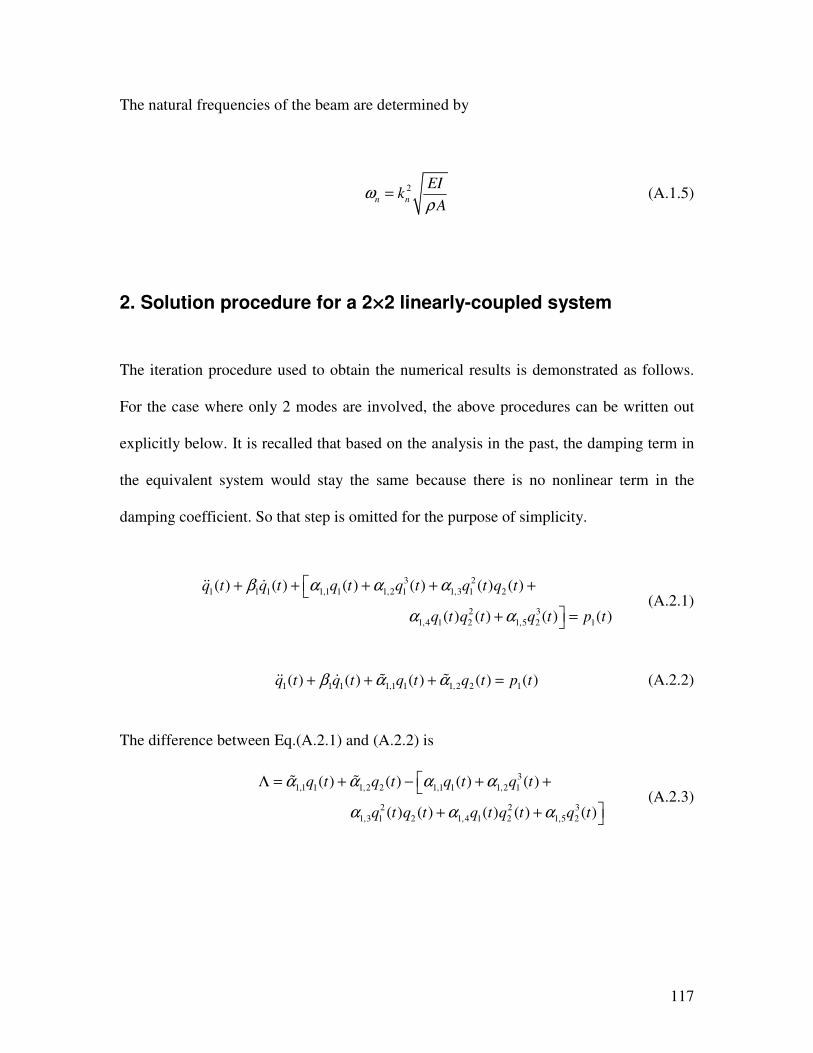
117

The natural frequencies of the beam are determined by

2

n n

EIk

Aω

ρ= (A.1.5)

2. Solution procedure for a 2¥2 linearly-coupled system

The iteration procedure used to obtain the numerical results is demonstrated as follows.

For the case where only 2 modes are involved, the above procedures can be written out

explicitly below. It is recalled that based on the analysis in the past, the damping term in

the equivalent system would stay the same because there is no nonlinear term in the

damping coefficient. So that step is omitted for the purpose of simplicity.

3 2

1 1 1 1,1 1 1,2 1 1,3 1 2

2 3

1,4 1 2 1,5 2 1

( ) ( ) ( ) ( ) ( ) ( )

( ) ( ) ( ) ( )

q t q t q t q t q t q t

q t q t q t p t

β α α α

α α

+ + + + +

+ =

(A.2.1)

1 1 1 1,1 1 1,2 2 1( ) ( ) ( ) ( ) ( )q t q t q t q t p tβ α α+ + + = (A.2.2)

The difference between Eq.(A.2.1) and (A.2.2) is

3

1,1 1 1,2 2 1,1 1 1,2 1

2 2 3

1,3 1 2 1,4 1 2 1,5 2

( ) ( ) ( ) ( )

( ) ( ) ( ) ( ) ( )

q t q t q t q t

q t q t q t q t q t

α α α α

α α α

Λ = + − + +

+ +

(A.2.3)

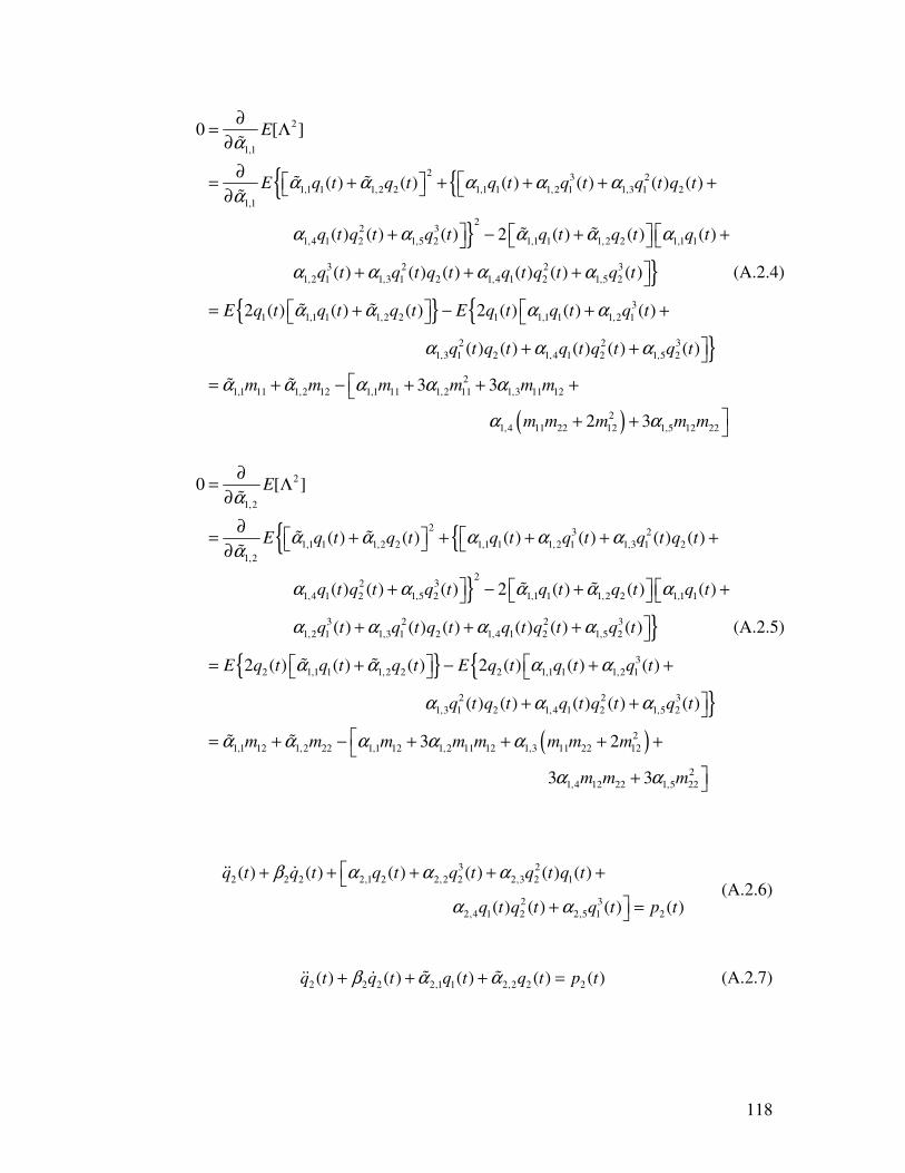
118

2

1,1

2 3 2

1,1 1 1,2 2 1,1 1 1,2 1 1,3 1 2

1,1

22 3

1,4 1 2 1,5 2 1,1 1 1,2 2 1,1 1

3 2 2

1,2 1 1,3 1 2 1,4 1 2

0 [ ]

( ) ( ) ( ) ( ) ( ) ( )

( ) ( ) ( ) 2 ( ) ( ) ( )

( ) ( ) ( ) ( ) ( )

E

E q t q t q t q t q t q t


q t q t q t q t q t

α

α α α α αα

α α α α α

α α α

∂= Λ

∂

∂ = + + + + + ∂

+ − + +

+ + +

( )

3

1,5 2

3

1 1,1 1 1,2 2 1 1,1 1 1,2 1

2 2 3

1,3 1 2 1,4 1 2 1,5 2

2

1,1 11 1,2 12 1,1 11 1,2 11 1,3 11 12

2

1,4 11 22 12 1,5 12 22

( )

2 ( ) ( ) ( ) 2 ( ) ( ) ( )

( ) ( ) ( ) ( ) ( )

3 3

2 3

q t

E q t q t q t E q t q t q t

q t q t q t q t q t

m m m m m m

m m m m m

α

α α α α

α α α

α α α α α

α α

= + − + +

+ +

= + − + + +

+ +

(A.2.4)

2

1,2

2 3 2

1,1 1 1,2 2 1,1 1 1,2 1 1,3 1 2

1,2

22 3

1,4 1 2 1,5 2 1,1 1 1,2 2 1,1 1

3 2 2

1,2 1 1,3 1 2 1,4 1 2

0 [ ]

( ) ( ) ( ) ( ) ( ) ( )

( ) ( ) ( ) 2 ( ) ( ) ( )

( ) ( ) ( ) ( ) ( )

E

E q t q t q t q t q t q t


q t q t q t q t q t

α

α α α α αα

α α α α α

α α α

∂= Λ

∂

∂ = + + + + + ∂

+ − + +

+ + +

( )

3

1,5 2

3

2 1,1 1 1,2 2 2 1,1 1 1,2 1

2 2 3

1,3 1 2 1,4 1 2 1,5 2

2

1,1 12 1,2 22 1,1 12 1,2 11 12 1,3 11 22 12

2

1,4 12 22 1,5 22

( )

2 ( ) ( ) ( ) 2 ( ) ( ) ( )

( ) ( ) ( ) ( ) ( )

3 2

3 3

q t

E q t q t q t E q t q t q t

q t q t q t q t q t

m m m m m m m m

m m m

α

α α α α

α α α

α α α α α

α α

= + − + +

+ +

= + − + + + +

+

(A.2.5)

3 2

2 2 2 2,1 2 2,2 2 2,3 2 1

2 3

2,4 1 2 2,5 1 2

( ) ( ) ( ) ( ) ( ) ( )

( ) ( ) ( ) ( )


q t q t q t p t

β α α α

α α

+ + + + +

+ =

(A.2.6)

2 2 2 2,1 1 2,2 2 2( ) ( ) ( ) ( ) ( )q t q t q t q t p tβ α α+ + + = (A.2.7)

119

The difference between Eq.(A.2.6) and (A.2.7) is

3

2,1 1 2,2 2 2,1 2 2,2 2

2 2 3

2,3 2 1 2,4 1 2 2,5 1

( ) ( ) ( ) ( )

( ) ( ) ( ) ( ) ( )

q t q t q t q t

q t q t q t q t q t

α α α α

α α α

Λ = + − + +

+ +

(A.2.8)

Similarly, we can obtain another two equations to solve for 2,1 2,2 and α α by setting

2 2

2,1 2,2

[ ] 0 and [ ] 0E Eα α∂ ∂

Λ = Λ =∂ ∂

.

To summarize, we have the following four equations to solve for 1,1 1,2 2,1 2,2, , , α α α α

( )( )

2 2

1,1 11 1,2 12 1,1 11 1,2 11 1,3 11 12 1,4 11 22 12 1,5 12 22

2 2

1,1 12 1,2 22 1,1 12 1,2 11 12 1,3 11 22 12 1,4 12 22 1,5 22

2,1 12 2,2 22 2,1 22 2,2 22

0 3 3 2 3

0 3 2 3 3

0 3

m m m m m m m m m m m


m m m m

α α α α α α α


α α α α

= + − + + + + +

= + − + + + + +

= + − +

( )( )

2 2

2,3 12 22 2,4 11 22 12 2,5 12 11

2 2

2,1 11 2,2 12 2,1 12 2,2 12 22 1,3 11 22 12 2,4 12 11 2,5 11

3 2 3

0 3 2 3 3

m m m m m m m


α α α


+ + + + = + − + + + + +

(A.2.9)

where by definition:

2

11 1

12 1 2

21 2 1 12

2

22 2

[ ( )]

[ ( ) ( )]

[ ( ) ( )]

[ ( )]

m E q t

m E q t q t

m E q t q t m

m E q t

=

=

= =

=

(A.2.10)

and they are calculated from the relationship

( ) ( )

( ) ( )

11 12 22

11 1

22 22 22

21 2

1( )

1( )

( )ij ij ii jj

m S d

m S d

m m m i j

ω ωω α β ω

ω ωω α β ω

ρ

∞

−∞

∞

−∞

=− +

=− +

= ≠

∫

∫

(A.2.11)

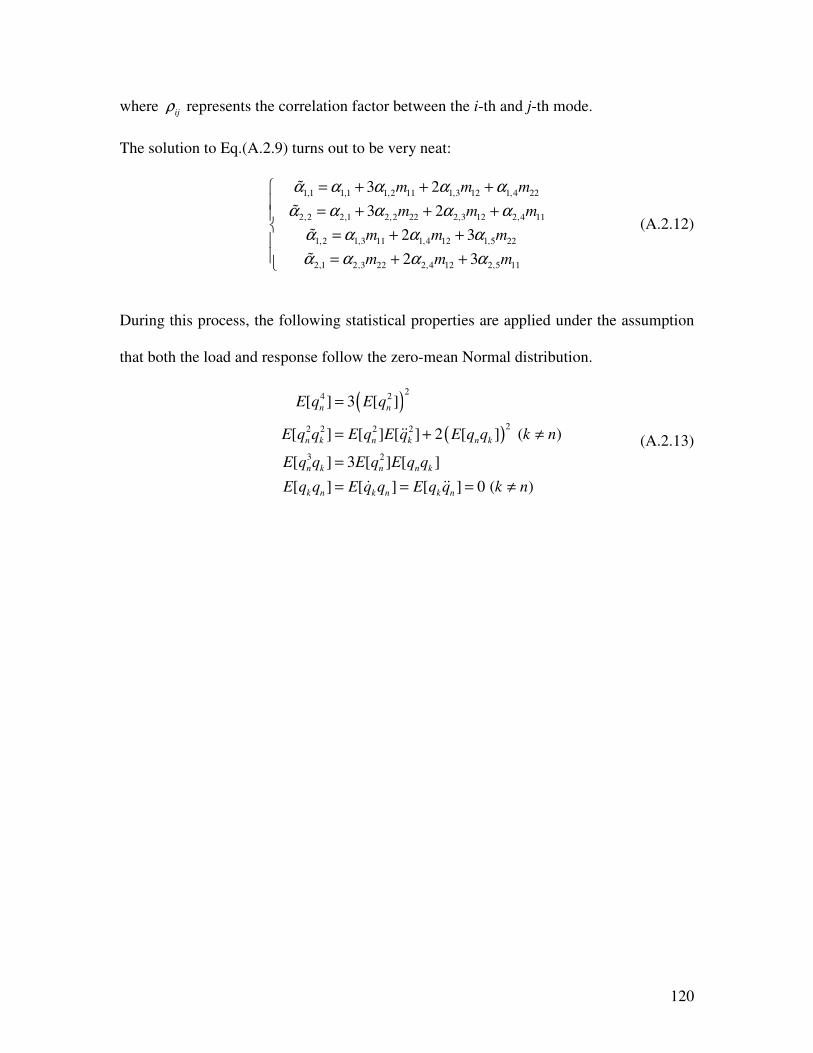
120

where ijρ represents the correlation factor between the i-th and j-th mode.

The solution to Eq.(A.2.9) turns out to be very neat:

1,1 1,1 1,2 11 1,3 12 1,4 22

2,2 2,1 2,2 22 2,3 12 2,4 11

1,2 1,3 11 1,4 12 1,5 22

2,1 2,3 22 2,4 12 2,5 11

3 2

3 2

2 3

2 3

m m m

m m m

m m m

m m m

α α α α α

α α α α αα α α α

α α α α

= + + + = + + + = + + = + +

(A.2.12)

During this process, the following statistical properties are applied under the assumption

that both the load and response follow the zero-mean Normal distribution.

( )( )

24 2

22 2 2 2

3 2

[ ] 3 [ ]

[ ] [ ] [ ] 2 [ ] ( )

[ ] 3 [ ] [ ]

[ ] [ ] [ ] 0 ( )

n n

n k n k n k

n k n n k

k n k n k n

E q E q

E q q E q E q E q q k n

E q q E q E q q

E q q E q q E q q k n

=

= + ≠

=

= = = ≠

(A.2.13)

121

Appendix B: Derivation of Plate Equations

Assume that there are no body force and no external loads.

For FSDT, it is assumed that

0

0

0

( , , , ) ( , , ) ( , , )

( , , , ) ( , , ) ( , , )

( , , , ) ( , , )

u x y z t u x y t z x y t

v x y z t v x y t z x y t

w x y z t w x y t

φ

ψ

= +

= +

=

(B.1)

where the subscript “0” represents the middle plane.

By definition, the strains that contain the von Carman nonlinear terms are

0 1

0 1

0 1

2

0 0

2

0 0

0 0 0 0

1

2

1

2

T

xx xx xx xx

T

yy yy yy yy

T

xy xy xy xy

z

u w

x xx

v wz

y y y

u v w w

y xy x x y

ε ε ε ε

ε ε ε ε

γ γ γ γ

φ

ψ

φ ψ

= + +

∂ ∂ ∂+ ∂ ∂ ∂ ∂ ∂ ∂

= + + ∂ ∂ ∂ ∂ ∂∂ ∂ ∂ ∂ ++ +

∂ ∂∂ ∂ ∂ ∂

0

0

( , , )

( , , )

( , , )

xx

yy

xy

xz

yz

T x y z

T x y z

T x y z

w

x

w

y

α

α

α

φγ

γψ

− ∆

+ − ∆ − ∆

∂ + ∂ = ∂ +

∂ (B.2)

122

The force and moment resultants on a plate element are shown below:

123

The strain energy of the plate element can be written as:

( )

0 0 0

1 1 1

0 0 0 1 1 1

xx xx yy yy xy xy xz xz yz yz

V

xx xx yy yy xy xy

xx xx yy yy xy xy x xz y yz xx xx yy yy xy xy

U

z z z dzdxdy

N N N V V M M M dxdy

σ ε σ ε τ γ τ γ τ γ

σ ε σ ε τ γ

ε ε γ γ γ ε ε εΩ

= + + + +

+ + +

= + + + + + + +

∫

∫

(B.3)

where, the force and moment resultants , ij ijN M can be obtained from the following

expressions for an orthotropic material:

0 1

11 12 16 11 12 16

0 1

12 22 26 12 22 26

0 1

16 26 66 16 26 66

xx xx xx

yy yy yy

xy xy xy

N A A A B B B

N A A A B B B

N A A A B B B

ε ε

ε εγ γ

= +

(B.4)

0 1

11 12 16 11 12 16

0 1

12 22 26 12 22 26

0 1

16 26 66 16 26 66

xx xx xx

yy yy yy

xy xy xy

M B B B D D D

M B B B D D D

M B B B D D D

ε ε

ε εγ γ

= +

(B.5)

44 45

45 55

( : shear correction factor)x

y

w

V A A x

wV A A

y

φκ κ

ψ

∂ + ∂ = ∂ +

∂

(B.6)

where,

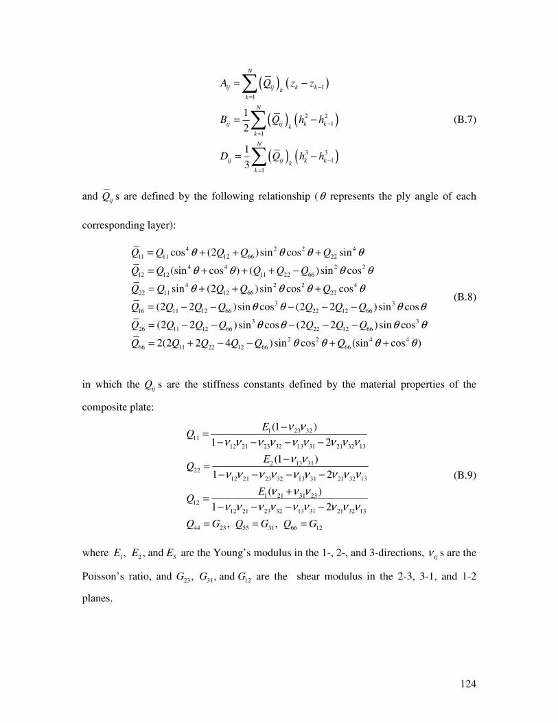
124

( ) ( )

( ) ( )

( ) ( )

1

1

2 2

1

1

3 3

1

1

1

2

1

3

N

ij ij k kkk

N

ij ij k kkk

N

ij ij k kkk

A Q z z

B Q h h

D Q h h

−

=

−

=

−

=

= −

= −

= −

∑

∑

∑

(B.7)

and ijQ s are defined by the following relationship (θ represents the ply angle of each

corresponding layer):

4 2 2 4

11 11 12 66 22

4 4 2 2

12 12 11 22 66

4 2 2 4

22 11 12 66 22

3 3

16 11 12 66 22 12 66

26 11 12 66

cos (2 )sin cos sin

(sin cos ) ( )sin cos

sin (2 )sin cos cos

(2 2 )sin cos (2 2 )sin cos

(2 2 )

Q Q Q Q Q

Q Q Q Q Q

Q Q Q Q Q

Q Q Q Q Q Q Q

Q Q Q Q

θ θ θ θ

θ θ θ θ

θ θ θ θ

θ θ θ θ

= + + +

= + + + −

= + + +

= − − − − −

= − − 3 3

22 12 66

2 2 4 4

66 11 22 12 66 66

sin cos (2 2 )sin cos

2(2 2 4 )sin cos (sin cos )

Q Q Q

Q Q Q Q Q Q

θ θ θ θ

θ θ θ θ

− − −

= + − − + +

(B.8)

in which the ij

Q s are the stiffness constants defined by the material properties of the

composite plate:

1 23 3211

12 21 23 32 13 31 21 32 13

2 13 3122

12 21 23 32 13 31 21 32 13

1 21 31 2312

12 21 23 32 13 31 21 32 13

44 23 55 31 66 12

(1 )

1 2

(1 )

1 2

( )

1 2

, ,

EQ

EQ

EQ

Q G Q G Q G

ν νν ν ν ν ν ν ν ν ν

ν νν ν ν ν ν ν ν ν ν

ν ν νν ν ν ν ν ν ν ν ν

−=

− − − −

−=

− − − −

+=

− − − −

= = =

(B.9)

where 1 2 3, , and E E E are the Young’s modulus in the 1-, 2-, and 3-directions, ij

ν s are the

Poisson’s ratio, and 23 31 12, , and G G G are the shear modulus in the 2-3, 3-1, and 1-2

planes.

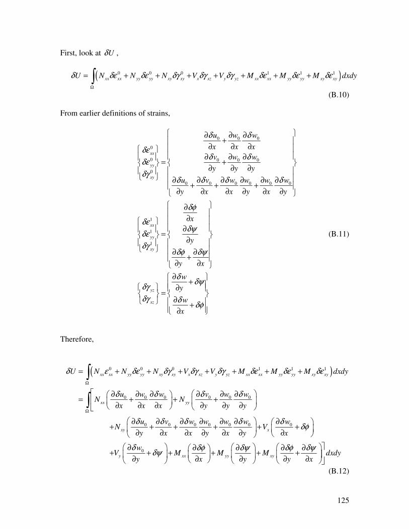
125

First, look at Uδ ,

( )0 0 0 1 1 1

xx xx yy yy xy xy x xz y yz xx xx yy yy xy xyU N N N V V M M M dxdyδ δε δε δγ δγ δγ δε δε δεΩ

= + + + + + + +∫ (B.10)

From earlier definitions of strains,

0 0 0

0

0 0 0 0

0

0 0 0 0 0 0

1

1

1

xx

yy

xy

xx

yy

xy

yz

xz

u w w

x x x

v w w

y y y

u v w w w w

y x x y x y

x

y

y x

w

δ δ

δεδ δ

δε

δγδ δ δ δ

δφ

δεδψ

δεδγ

δφ δψ

δδγ

δγ

∂ ∂ ∂+

∂ ∂ ∂ ∂ ∂ ∂

= + ∂ ∂ ∂

∂ ∂ ∂ ∂ ∂ ∂+ + +

∂ ∂ ∂ ∂ ∂ ∂

∂

∂ ∂

= ∂

∂ ∂+

∂ ∂

∂

=

y

w

x

δψ

δδφ

+ ∂

∂ + ∂

(B.11)

Therefore,

( )0 0 0 1 1 1

0 0 0 0 0 0

0 0 0 0 0 0 0

xx xx yy yy xy xy x xz y yz xx xx yy yy xy xy

xx yy

xy x

U N N N V V M M M dxdy

u w w v w wN N

x x x y y y

u v w w w w wN V

y x x y x y x

δ ε δε δγ δγ δγ δε δε δε

δ δ δ δ

δ δ δ δ δδφ

Ω

Ω

= + + + + + + +

∂ ∂ ∂ ∂ ∂ ∂ = + + + ∂ ∂ ∂ ∂ ∂ ∂

∂ ∂ ∂ ∂ ∂ ∂ ∂ + + + + + + ∂ ∂ ∂ ∂ ∂ ∂ ∂

∫

∫

0y xx yy xy

wV M M M dxdy

y x y y x

δ δφ δψ δφ δψδψ

∂ ∂ ∂ ∂ ∂ + + + + + + ∂ ∂ ∂ ∂ ∂ (B.12)

126

Now integrating by parts, one has

( ) ( ) ( ) ( ) ( )

( ) ( )

( )

0 0 0 00 0 0 0 0 0 0 0

0 0

0 00 0 0 0

0

xx yy xy

S

x y xx yy xy

yyxxxx yy

xy

w w w wU N u w N v w N u v w w

x y y x

V w V w M M M ds

NN w wu N w v N w

x x x y y y

Nv

x

δ δ δ δ δ δ δ δ δ

δ δ δφ δψ δφ δψ

δ δ δ δ

δ

Ω

∂ ∂ ∂ ∂ = + + + + + + + ∂ ∂ ∂ ∂

+ + + + + +

∂ ∂ ∂ ∂∂ ∂ − + + + ∂ ∂ ∂ ∂ ∂ ∂

∂+

∂

∫

∫

( )

( ) ( ) ( )

( ) ( ) ( ) ( )

( ) ( )

0 00 0 0

0 0

0 0 0 00 0 0

xy

xy xy

yxx y

yy xy xyxx

xx xy yy xy xx yy xy x y

Nw wN w u N w

x y y y x

VVw w V V

x y

M M MMdxdy

x y y x

w w w wu N N v N N w N N N V V

x y y x

δ δ δ

δ δ δφ δψ

δφ δψ δφ δψ

δ δ δ

∂ ∂ ∂∂ ∂ + + + ∂ ∂ ∂ ∂ ∂

∂∂+ + − +

∂ ∂

∂ ∂ ∂ ∂+ + + + ∂ ∂ ∂ ∂

∂ ∂ ∂ ∂= + + + + + + + + + ∂ ∂ ∂ ∂

( ) ( )

0 0

0 0 0 00

S

xx xy yy xy

xy xy yyxx

yxxx xy xy yy

xy xy yyxxx y

M M M M ds

N N NNu v

x y x y

VV w w w ww N N N N

x y x x y y y y

M M MMV V

x y x

δφ δψ

δ δ

δ

δφ δψ

Ω

+ + + +

∂ ∂ ∂ ∂− + + + ∂ ∂ ∂ ∂

∂ ∂ ∂ ∂ ∂ ∂∂ ∂+ + + + + + ∂ ∂ ∂ ∂ ∂ ∂ ∂ ∂

∂ ∂ ∂ ∂+ − + + + − + + ∂ ∂ ∂

∫

∫

dxdyy

∂

(B.13)

On the other hand, the strain energy associated with the thermal stresses is:

( )0 0 0 1 1 1T T T T T T T

xx xx yy yy xy xy xx xx yy yy xy xyU N N N M M M dxdyε ε γ ε ε εΩ

= + + + + +∫ (B.14)

where the subscript T represents the force/moment caused by thermal effects, and

, T T

ij ijN M are determined by

127

111 12

12 22

166

11 12

12 22

66

0 ( , , )

0 ( , , )

0 0 ( , , )

0 ( , , )

0 ( , , )

0 0

k

k

T

xx xxN zT

yy yyzT k

xy xyk

T

xx xx

T

yy yy

T

xy xyk

N Q Q T x y z

N Q Q T x y z dz

Q T x y z

M Q Q T x y z

M Q Q T x y z

M Q

α

α

γ α

α

α

α

+

=

− ∆ = − ∆ − ∆

− ∆ = − ∆ − ∆

∑∫

1

1 ( , , )

k

k

N z

zk

zdz

T x y z

+

=

∑∫

(B.15)

For TUδ , following the same procedure as that in the derivation of Uδ , one obtains

( )

( ) ( ) ( )

0 0 0 1 1 1

0 0 0 00 0 0 0 0 0 0 0

0

T T T T T T T

xx xx yy yy xy xy xx xx yy yy xy xy

T T T

xx yy xy

S

T T T

xx yy xy

Txyxx

U N N N M M M dxdy

w w w wN u w N v w N u v w w

x y y x

M M M ds

NNu

x

δ δε δε δγ δε δε δε

δ δ δ δ δ δ δ δ

δφ δψ δφ δψ

δ

Ω

= + + + + +

∂ ∂ ∂ ∂ = + + + + + + + ∂ ∂ ∂ ∂

+ + + +

∂∂− +

∂

∫

∫

0

0 0 0 00

T T T

xy yy

T T T T

xx xy xy yy

T T TTxy xy yyxx

N Nv

y x y

w w w ww N N N N

x x y y y y

M M MMdxdy

x y x y

δ

δ

δφ δψ

Ω

∂ ∂+ + ∂ ∂ ∂

∂ ∂ ∂ ∂∂ ∂+ + + + ∂ ∂ ∂ ∂ ∂ ∂

∂ ∂ ∂∂ + + + + ∂ ∂ ∂ ∂

∫

(B.16)

The kinetic energy of the plate element is

( )

( )

2 2 2

0 0 0 0 0 0

1

2

( ) ( ) ( ) ( )

V

V

V

K u v w dV

K u u v v w w dV

u z u z v z v z w w dV

ρ

δ ρ δ δ δ

ρ φ δ δφ ρ ψ δ δψ ρ δ

= + +

= ⋅ + ⋅ + ⋅

= + ⋅ + + + ⋅ + + ⋅

∫

∫

∫

(B.17)

128

()

0 0 0 0 0 0

2

0 0 0 0 0 0

2

0 0 0

( ) ( ) ( ) ( )

V

u z u z v z v z w w dzdxdy

dz u u zdz u zdz u z dz dz v v

zdz v zdz v z dz dz w w dxdy

ρ φ δ δφ ρ ψ δ δψ ρ δ

ρ δ ρ δφ ρ φδ ρ φδφ ρ δ

ρ δψ ρ ψδ ρ ψδψ ρ δ

Ω

= + ⋅ + + + ⋅ + + ⋅

= ⋅ + ⋅ + ⋅ + ⋅ + ⋅

+ ⋅ + ⋅ + ⋅ + ⋅

∫

∫ ∫ ∫ ∫ ∫ ∫

∫ ∫ ∫ ∫

Define,

2

0 1 2, , I dz I zdz I z dzρ ρ ρ= = =∫ ∫ ∫ (B.18)

Therefore,

()

(

2

0 0 0 0 0 0

2

0 0 0 0

0 0 0 1 0 1 0 2 0 0 0 1 0 1 0

2

K dz u u zdz u zdz u z dz dz v v

zdz v zdz v z dz dz w w dxdy

I u u I u I u I I v v I v I v

I

δ ρ δ ρ δφ ρ φδ ρ φδφ ρ δ

ρ δψ ρ ψδ ρ ψδψ ρ δ

δ δφ φδ φδφ δ δψ ψδ

ψδψ

Ω

Ω

= ⋅ + ⋅ + ⋅ + ⋅ + ⋅

+ ⋅ + ⋅ + ⋅ + ⋅

= + + + + + +

+ +

∫ ∫ ∫ ∫ ∫ ∫

∫ ∫ ∫ ∫∫

)0 0 0I w w dxdyδ

(B.19)

Integration by parts with respect to time t leads to

(

)

( ) ( ) ( )

( )

0 0 0 1 0 1 0 2 0 0 0 1 0 1 0

2 0 0 0

0 0 0 1 0 0 0 1 0 0 0 2 1 0

1 0 2

0 0 0 1 0 1 0 2 0

S

K I u u I u I u I I v v I v I v

I I w w dxdy

u I u I v I v I I w w I I u

I v I ds

I u u I u I u I I

δ δ δφ φδ φδφ δ δψ ψδ

ψδψ δ

δ φ δ ψ δ δφ φ

δψ ψ

δ δφ φδ φδφ

Ω

= + + + + + +

+ +

= + + + + + +

+ +

− + + + +

∫

∫

(

)

(

)

0 0 1 0

1 0 2 0 0 0

0 0 0 1 0 1 0 2 0 0 0 1 0 1 0

2 0 0 0

S

v v I v

I v I I w w dxdy

I u u I u I u I I v v I v I v

I I w w ds

δ δψ

ψδ ψδψ δ

δ δφ φδ φδφ δ δψ ψδ

ψδψ δ

Ω

+

+ + +

= + + + + + +

+ +

∫

∫

129

( ) ( ) ( )

( ) ( )

0 0 0 1 0 0 0 1 0 0 0

1 0 2 1 0 2

u I u I v I v I w I w

I u I I v I dxdy

δ φ δ ψ δ

δφ φ δψ ψ

Ω

− + + + +

+ + + +

∫

(B.20)

Substituting the expressions of Uδ , TUδ and Kδ into the virtual displacement

condition 0TU U Kδ δ δ+ − = and collecting similar terms, one has

( ) ( ) 0 0 0 1 0 0 0 1

0 0 0 0 0 00

0 00

T T T T T

xx xy xx xy yy xy yy xy

S

T T

xx yy xy xx yy

T

xy x y

U U K u N N N N I u I v N N N N I v I

w w w w w ww N N N N N

x y y x x y

w wN V V I w

y x

δ δ δ δ φ δ ψ

δ

+ − = + + + + + + + + + + +

∂ ∂ ∂ ∂ ∂ ∂ + + + + + + ∂ ∂ ∂ ∂ ∂ ∂

∂ ∂+ + + + + ∂ ∂

∫

( ) ( )

0

2 1 0 1 0 2

0 0 0 1

0 0 0 1

0

T T T T


TTxy xyxx xx

T T

xy yy xy yy

yx

M M M M I I u M M M M I v I ds

N NN Nu I u I

x y x y

N N N Nv I v I

x y x y

VVw

x y

δφ φ δψ ψ

δ φ

δ ψ

δ

Ω

+ + + + + + + + + + + +

∂ ∂∂ ∂− + + + − − ∂ ∂ ∂ ∂

∂ ∂ ∂ ∂+ + + + − − ∂ ∂ ∂ ∂

∂∂ ∂+ + +

∂ ∂

∫

0 0 0 0

0 0 0 00 0

1 0 2

T T

xx xy xx xy

T T

xy yy xy yy

TTxy xyxx xx

x

T T

xy yy xy yy

y

w w w wN N N N

x x y x y

w w w wN N N N I w

y y y y y

M MM MV I u I

x y x y

M M M MV I

x y x y

δφ φ

δψ

∂ ∂ ∂ ∂+ + + ∂ ∂ ∂ ∂ ∂

∂ ∂ ∂ ∂∂+ + + + − ∂ ∂ ∂ ∂ ∂

∂ ∂∂ ∂+ − + + + + − − ∂ ∂ ∂ ∂

∂ ∂ ∂ ∂+ − + + + + −

∂ ∂ ∂ ∂

1 0 2v I dxdyψ

−

(B.21)

130

Since the selections of 0 0 0, , , , and u v wδ δ δ δφ δψ are arbitrary, the coefficients of

0 0 0, , , , and u v wδ δ δ δφ δψ in the above expression must be zero, respectively. This

yields the governing equations of the plate

2 2

00 12 2

2 2

00 12 2

0 0 0 0

0 0 0 0

TTxy xyxx xx

T T

xy yy xy yy

y T Txxx xy xx xy

T T

xy yy xy yy

N NN N uI I

x y x y t t

N N N N vI I

x y x y t t

VV w w w wN N N N

x y x x y x y

w w w wN N N N

y x y y y

φ

ψ

∂ ∂∂ ∂ ∂ ∂+ + + = +

∂ ∂ ∂ ∂ ∂ ∂

∂ ∂ ∂ ∂ ∂ ∂+ + + = +

∂ ∂ ∂ ∂ ∂ ∂

∂ ∂ ∂ ∂ ∂ ∂∂+ + + + + ∂ ∂ ∂ ∂ ∂ ∂ ∂

∂ ∂ ∂ ∂∂+ + + +∂ ∂ ∂ ∂ ∂

2

00 2

22

02 12 2

22

02 12 2

TTxy xyxx xx

x

T T

xy yy xy yy

y

wI

t

M MM M uV I I

x y x y t t

M M M M vV I I

x y x y t t

φ

ψ

∂= ∂

∂ ∂∂ ∂ ∂∂+ + + − = +

∂ ∂ ∂ ∂ ∂ ∂

∂ ∂ ∂ ∂ ∂∂+ + + − = +

∂ ∂ ∂ ∂ ∂ ∂

(B.22)

with the boundary conditions coming from line integrals:

( ) ( ) 0 0 0 1 0 0 0 1

0 0 0 0 0 00

0 00 0

0 T T T T


S

T T

xx yy xy xx yy

T

xy x y

u N N N N I u I v N N N N I v I

w w w w w ww N N N N N

x y y x x y

w wN V V I w

y x

M

δ φ δ ψ

δ

δφ

= + + + + + + + + + + +

∂ ∂ ∂ ∂ ∂ ∂ + + + + + + ∂ ∂ ∂ ∂ ∂ ∂

∂ ∂+ + + + + ∂ ∂

+

∫

( ) ( )2 1 0 1 0 2

T T T T

xx xy xx xy yy xy yy xyM M M I I u M M M M I v I dsφ δψ ψ+ + + + + + + + + + +

(B.23)

random vibration analysis of higher-order nonlinear … · random vibration analysis of higher ......

Documents