randal koster gmao, nasa/gsfc …cola.gmu.edu/lsm/koster_s2_lsm.pdfrandal koster gmao, nasa/gsfc...
TRANSCRIPT


Reasoning (and assumptions) behind this talk’s emphasis:
1. We are interested in how soil moisture variations may feed back on the
atmosphere soil moisture as a potential source of predictability.
Reasoning (and assumptions) behind this talk’s emphasis:
1. We are interested in how soil moisture variations may feed back on the
atmosphere soil moisture as a potential source of predictability.
2. Soil moisture affects the overlying atmosphere mainly through its impact on
the surface energy balance.
3. Variations in the surface energy balance can be keyed, to first order, to
variations in evaporation (which, by the way, also lies at the heart of the surface
water balance).water balance).
4. Synoptic-scale variations in evaporation (the type that may influence
feedback) are tied to year-to-year variations in seasonally-averaged evaporation
– where one is high, so is the other. (Particularly assumed to be true for the soil
moisture-controlled component of evaporation – see later slide.)
5. Under these assumptions, we can look at the interannual variance of
seasonally-averaged evaporation to get a first-order handle on feedback
potential.
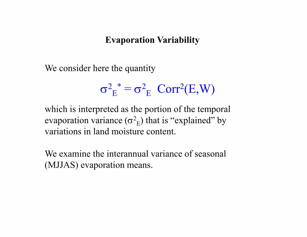
We consider here the quantity
σ2E* = σ2E Corr
2(E,W)
which is interpreted as the portion of the temporal
evaporation variance (σ2 ) that is “explained” by
Evaporation Variability
evaporation variance (σ2E) that is “explained” by
variations in land moisture content.
We examine the interannual variance of seasonal
(MJJAS) evaporation means.
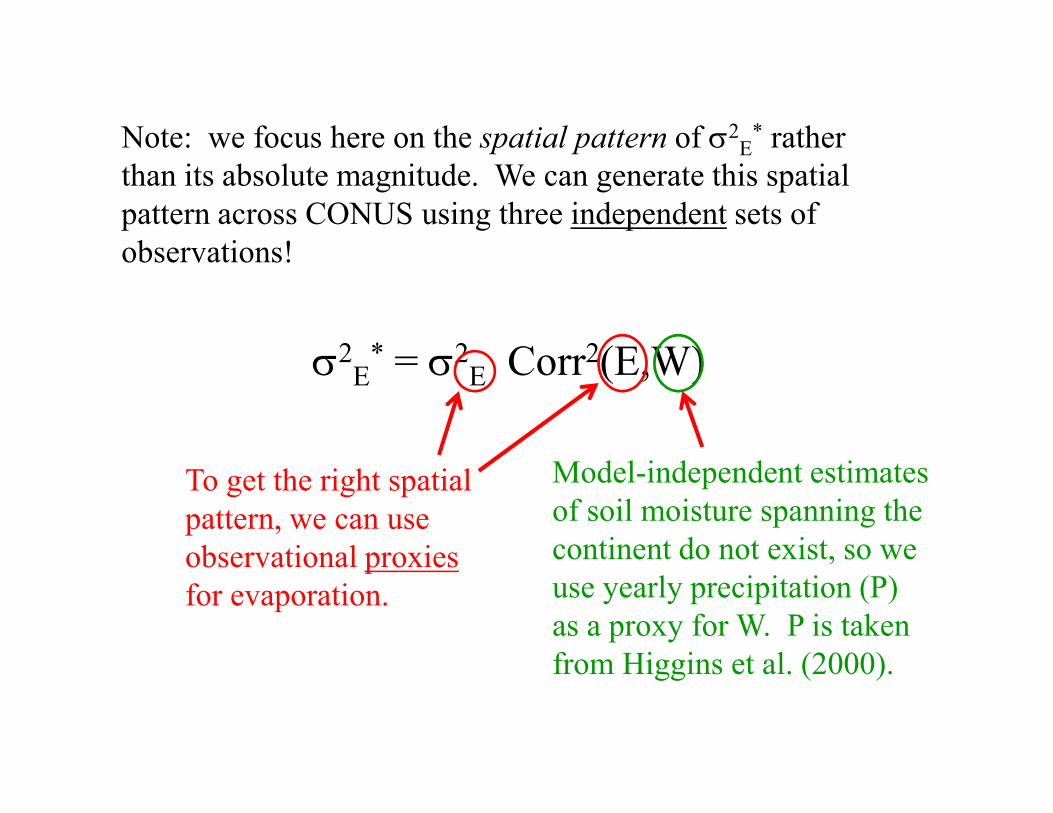
Note: we focus here on the spatial pattern of σ2E* rather
than its absolute magnitude. We can generate this spatial
pattern across CONUS using three independent sets of
observations!
σ2E* = σ2E Corr
2(E,W)
To get the right spatial
pattern, we can use
observational proxies
for evaporation.
Model-independent estimates
of soil moisture spanning the
continent do not exist, so we
use yearly precipitation (P)
as a proxy for W. P is taken
from Higgins et al. (2000).
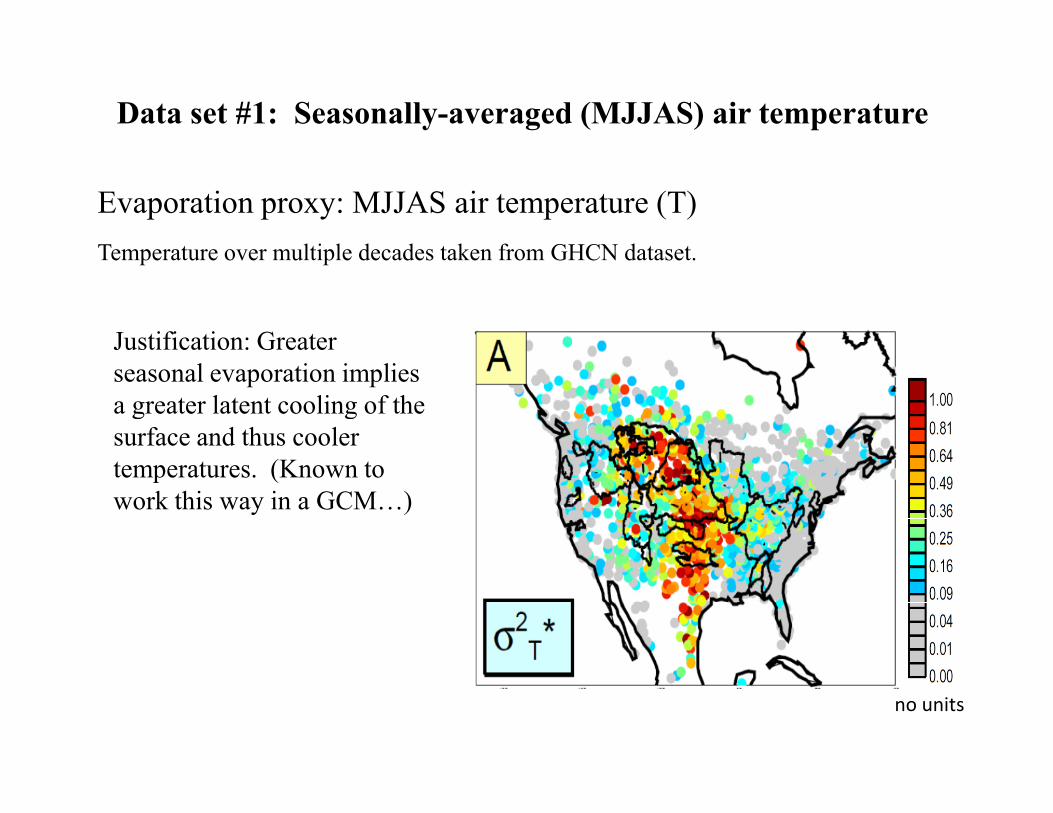
Data set #1: Seasonally-averaged (MJJAS) air temperature
Evaporation proxy: MJJAS air temperature (T)
Temperature over multiple decades taken from GHCN dataset.
Justification: Greater
seasonal evaporation implies
a greater latent cooling of the a greater latent cooling of the
surface and thus cooler
temperatures. (Known to
work this way in a GCM…)
no units
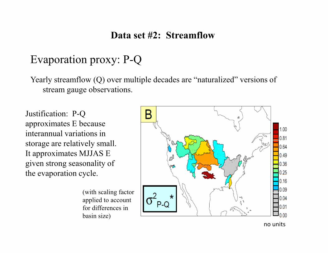
Data set #2: Streamflow
Evaporation proxy: P-Q
Yearly streamflow (Q) over multiple decades are “naturalized” versions of
stream gauge observations.
Justification: P-Q
approximates E because
(with scaling factor
applied to account
for differences in
basin size)
no units
approximates E because
interannual variations in
storage are relatively small.
It approximates MJJAS E
given strong seasonality of
the evaporation cycle.
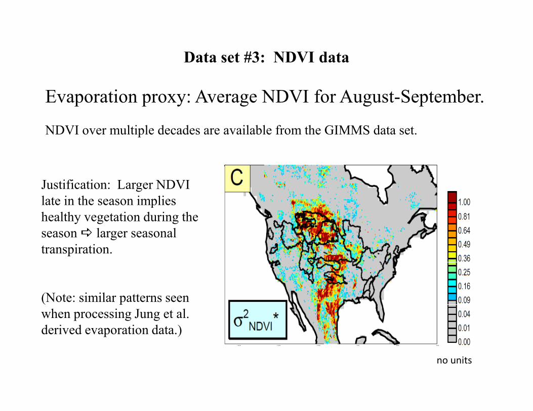
Data set #3: NDVI data
Evaporation proxy: Average NDVI for August-September.
NDVI over multiple decades are available from the GIMMS data set.
Justification: Larger NDVI
late in the season implies
no units
late in the season implies
healthy vegetation during the
season larger seasonal
transpiration.
(Note: similar patterns seen
when processing Jung et al.
derived evaporation data.)
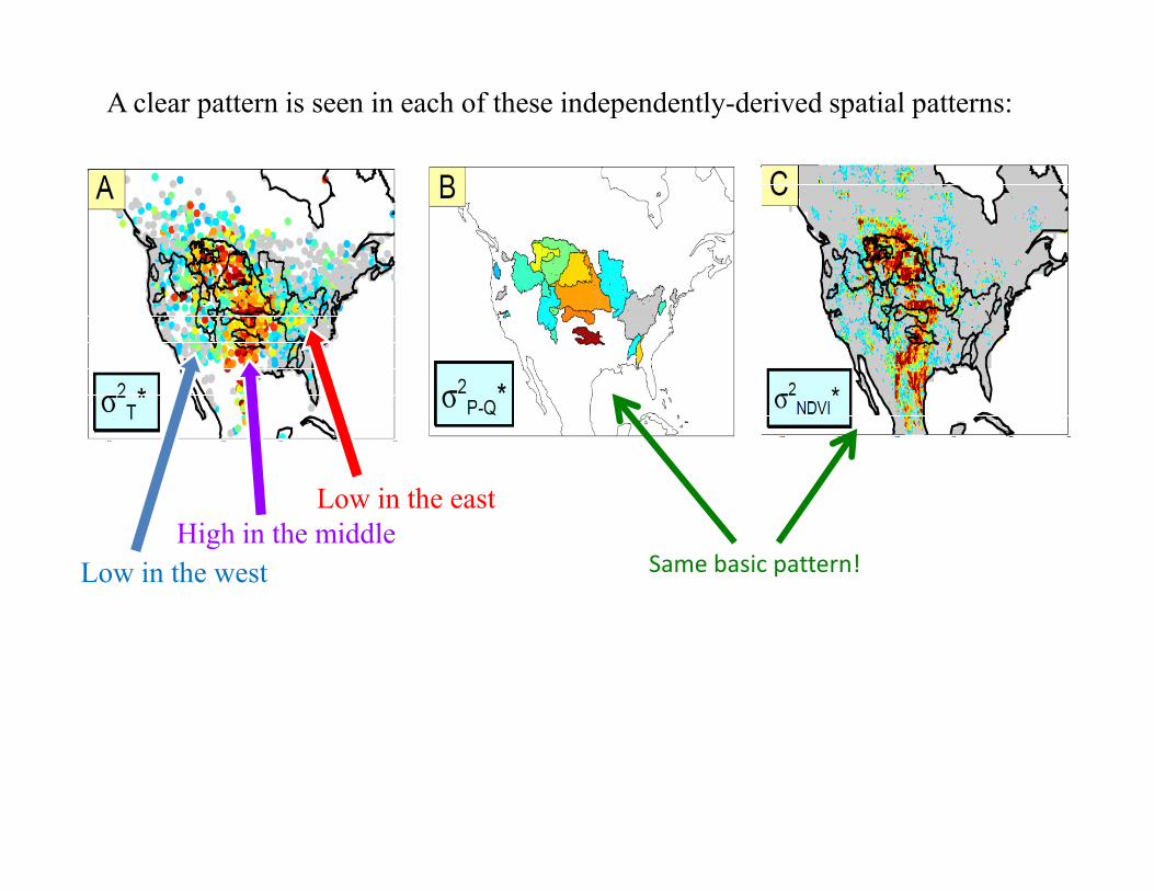
A clear pattern is seen in each of these independently-derived spatial patterns:
Low in the west
High in the middle
Low in the east
Same basic pattern!
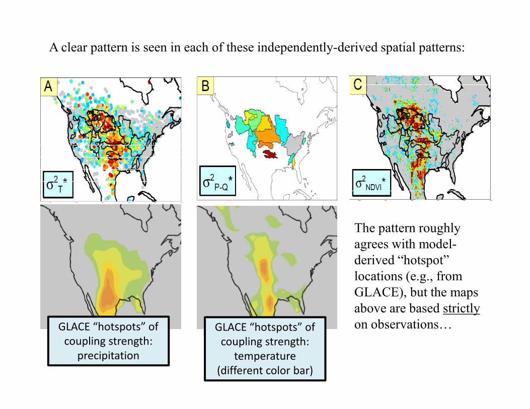
A clear pattern is seen in each of these independently-derived spatial patterns:
The pattern roughly
agrees with model-
derived “hotspot”
locations (e.g., from
GLACE), but the maps
above are based strictly
on observations…GLACE “hotspots” of
coupling strength:
temperature
(different color bar)
GLACE “hotspots” of
coupling strength:
precipitation
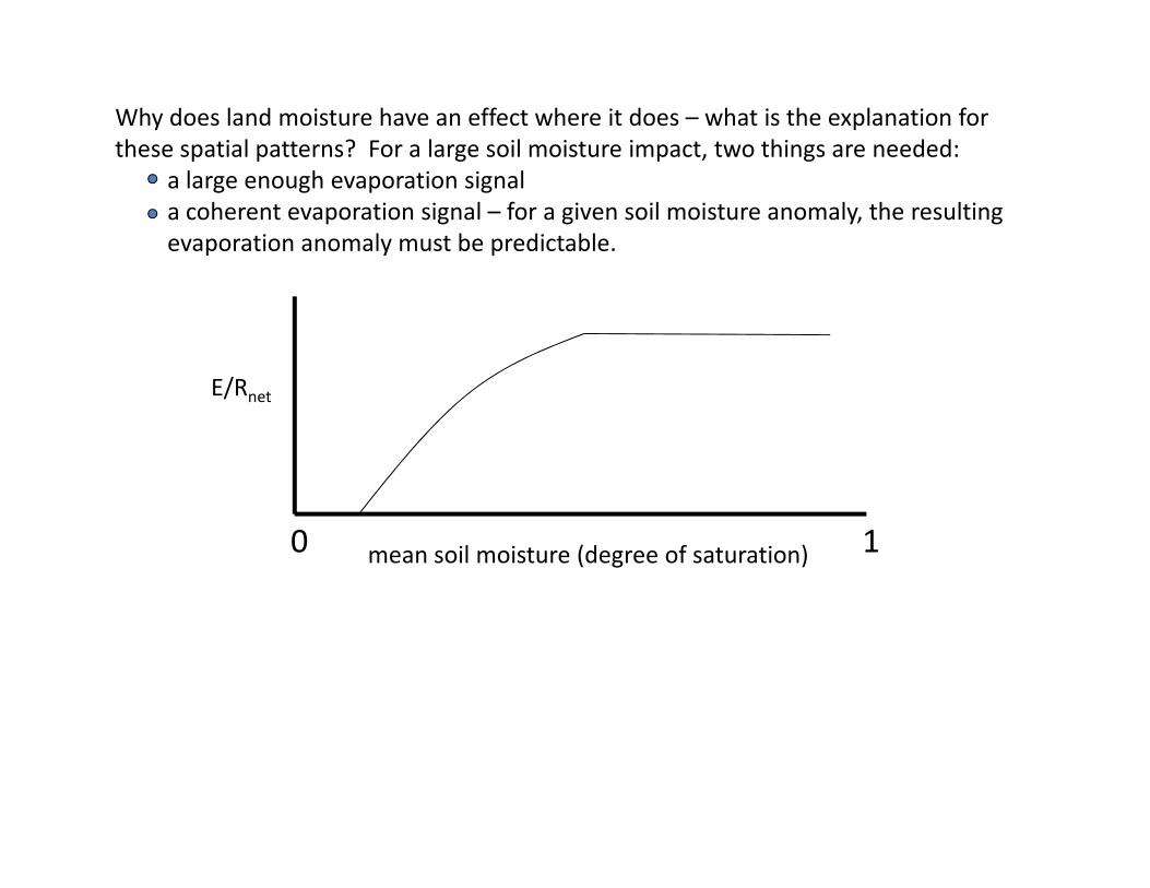
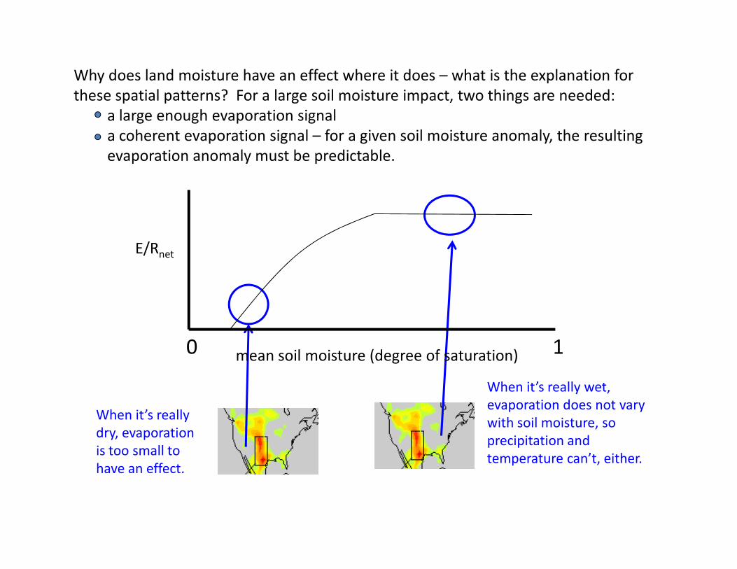
Why does land moisture have an effect where it does – what is the explanation for
these spatial patterns? For a large soil moisture impact, two things are needed:
a large enough evaporation signal
a coherent evaporation signal – for a given soil moisture anomaly, the resulting
evaporation anomaly must be predictable.
E/Rnet
mean soil moisture (degree of saturation)0 1
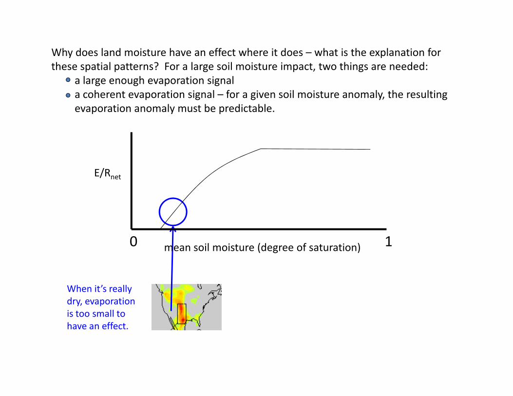
Why does land moisture have an effect where it does – what is the explanation for
these spatial patterns? For a large soil moisture impact, two things are needed:
a large enough evaporation signal
a coherent evaporation signal – for a given soil moisture anomaly, the resulting
evaporation anomaly must be predictable.
E/Rnet
When it’s really
dry, evaporation
is too small to
have an effect.
mean soil moisture (degree of saturation)0 1
Why does land moisture have an effect where it does – what is the explanation for
these spatial patterns? For a large soil moisture impact, two things are needed:
a large enough evaporation signal
a coherent evaporation signal – for a given soil moisture anomaly, the resulting
evaporation anomaly must be predictable.
E/Rnet
When it’s really
dry, evaporation
is too small to
have an effect.
When it’s really wet,
evaporation does not vary
with soil moisture, so
precipitation and
temperature can’t, either.
mean soil moisture (degree of saturation)0 1
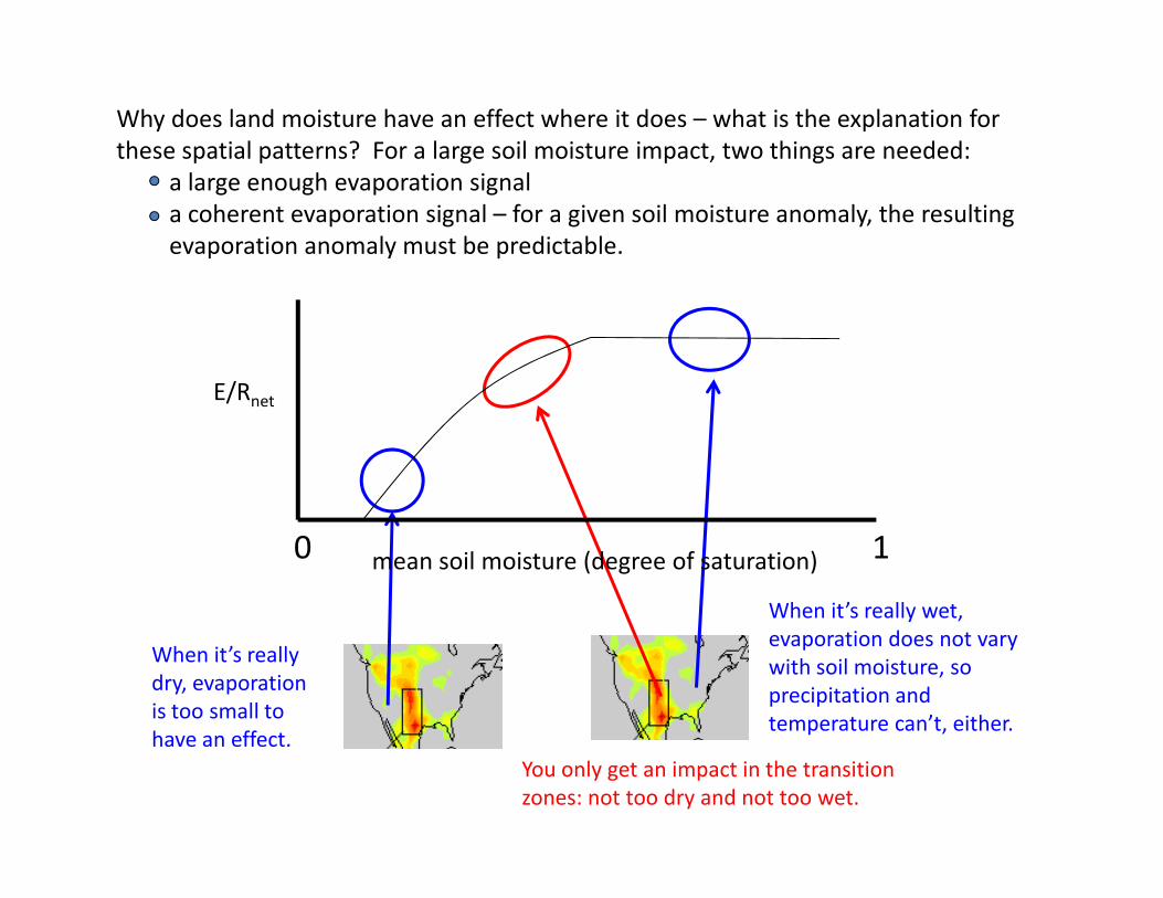
Why does land moisture have an effect where it does – what is the explanation for
these spatial patterns? For a large soil moisture impact, two things are needed:
a large enough evaporation signal
a coherent evaporation signal – for a given soil moisture anomaly, the resulting
evaporation anomaly must be predictable.
E/Rnet
When it’s really
dry, evaporation
is too small to
have an effect.
When it’s really wet,
evaporation does not vary
with soil moisture, so
precipitation and
temperature can’t, either.
You only get an impact in the transition
zones: not too dry and not too wet.
mean soil moisture (degree of saturation)0 1

How well do various LSMs do? Better than you might
think…
We examined simulation output produced by a number of
different state-of-the-art LSMs. Each LSM was driven different state-of-the-art LSMs. Each LSM was driven
offline over CONUS with multiple decades of observations-
based forcing.
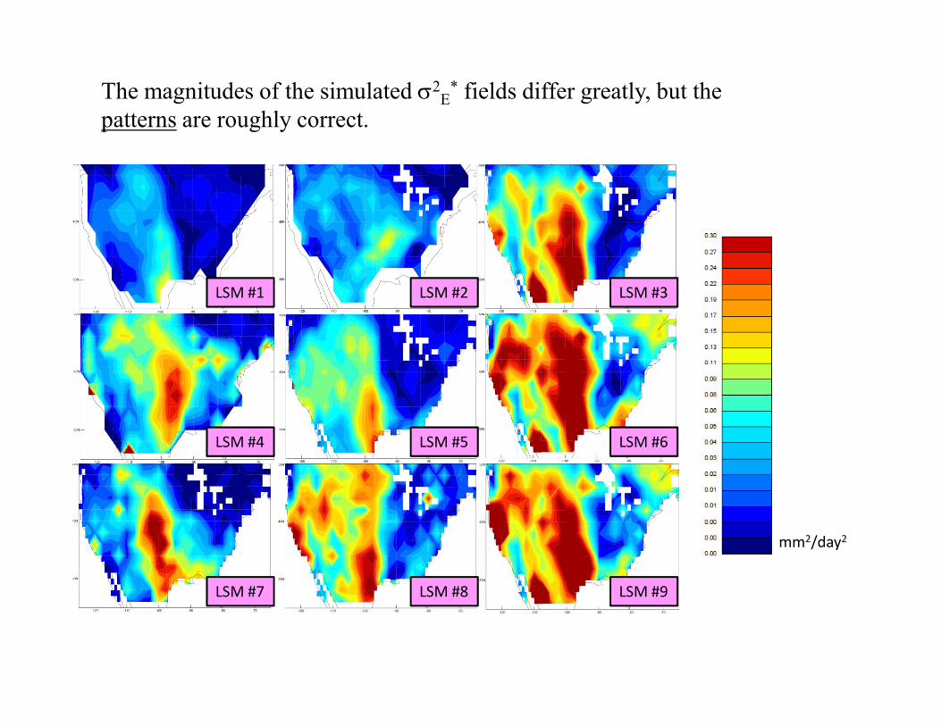
The magnitudes of the simulated σ2E* fields differ greatly, but the
patterns are roughly correct.
LSM #1 LSM #2 LSM #3
mm2/day2
LSM #4
LSM #7
LSM #5
LSM #8
LSM #6
LSM #9
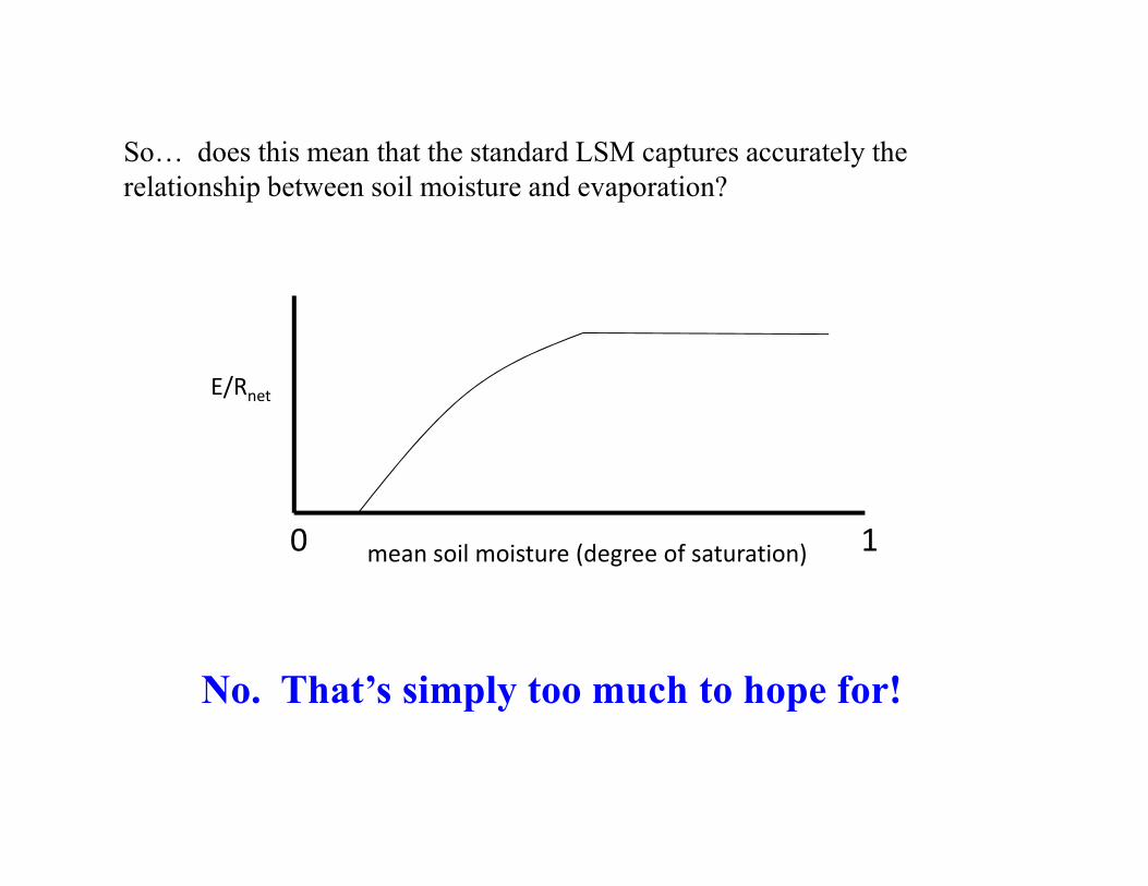
E/Rnet
So… does this mean that the standard LSM captures accurately the
relationship between soil moisture and evaporation?
mean soil moisture (degree of saturation)0 1
No. That’s simply too much to hope for!
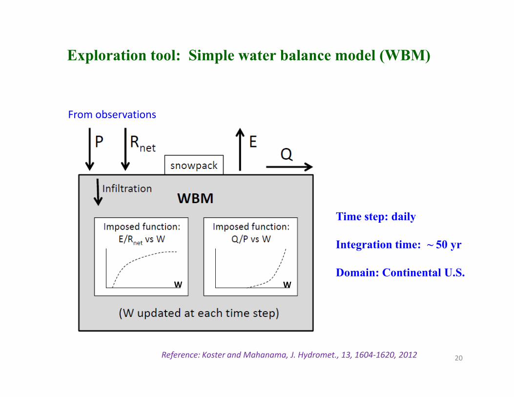
Exploration tool: Simple water balance model (WBM)
From observations
Time step: daily
Integration time: ~ 50 yr
Domain: Continental U.S.
20Reference: Koster and Mahanama, J. Hydromet., 13, 1604-1620, 2012
W W
Yes, this tool is simple:
The same functions are used everywhere within region studied
(e.g., ignoring spatial variability in vegetation and topography)
and at all times (e.g., ignoring seasonality in vegetation).
It lacks treatments of (for example) baseflow and interception
loss.
21
It lacks a treatment of the surface energy balance.
And so on… And so on…
Even so, we have found (Koster and Mahanama 2012) that it
successfully captures, to first order, the important controls on
hydroclimatic variability operating in a complex land surface
model and (presumably) in nature.
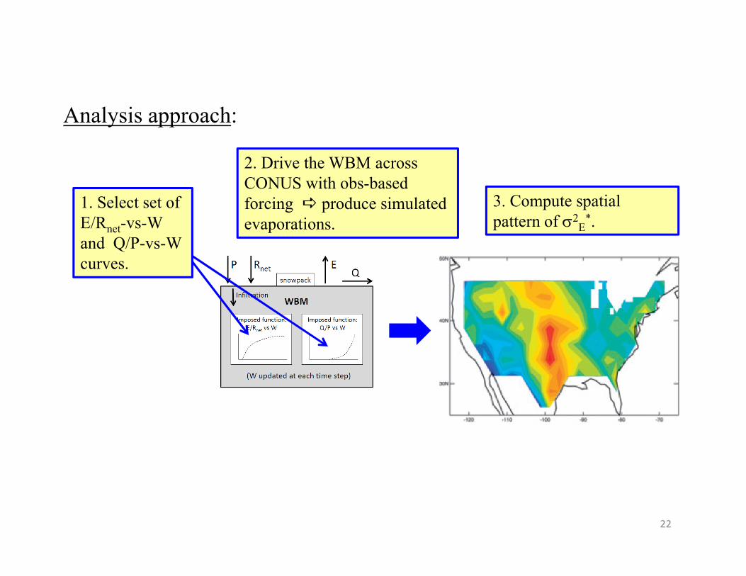
Analysis approach:
1. Select set of
E/Rnet-vs-W
and Q/P-vs-W
curves.
2. Drive the WBM across
CONUS with obs-based
forcing produce simulated
evaporations.
3. Compute spatial
pattern of σ2E*.
22
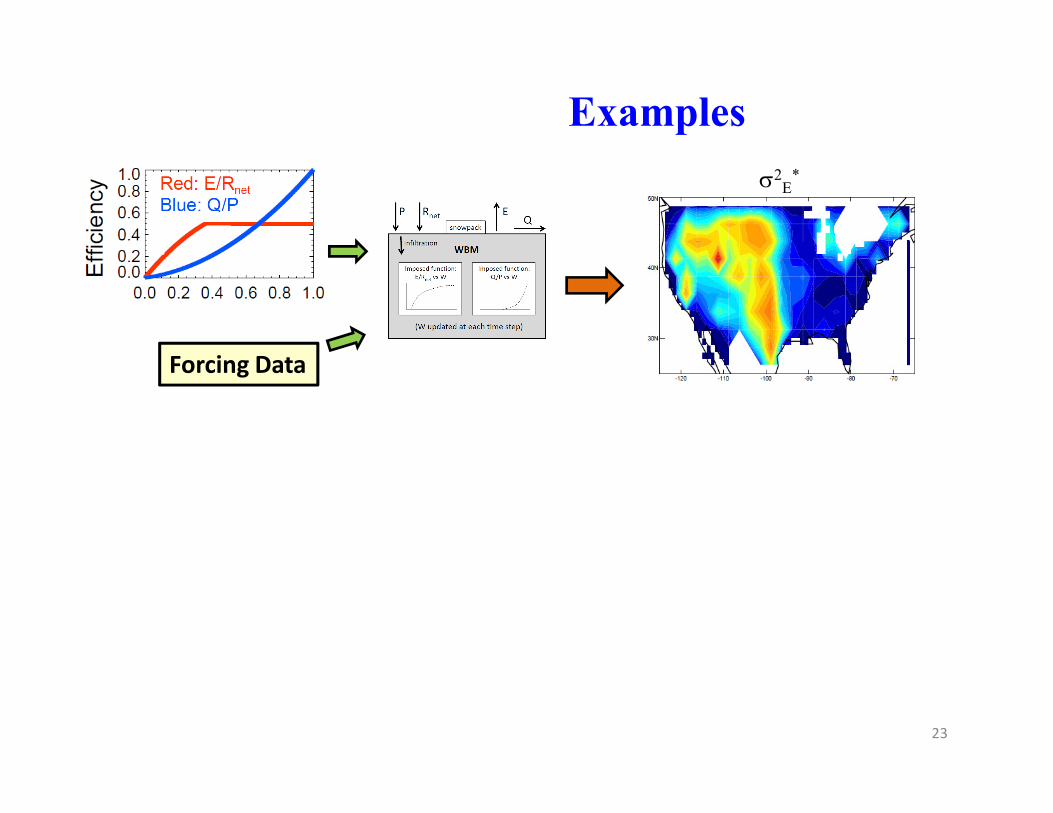
Examples
Forcing Data
σ2E*
23
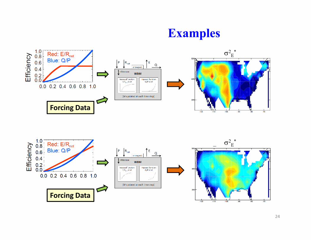
Examples
Forcing Data
σ2E*
24
Forcing Data
σ2E*
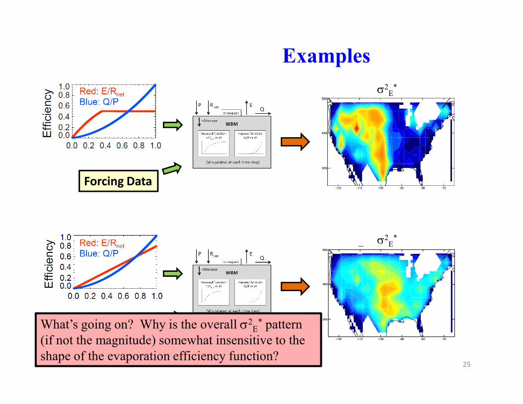
Examples
Forcing Data
σ2E*
25
Forcing DataWhat’s going on? Why is the overall σ2E* pattern
(if not the magnitude) somewhat insensitive to the
shape of the evaporation efficiency function?
σ2E*
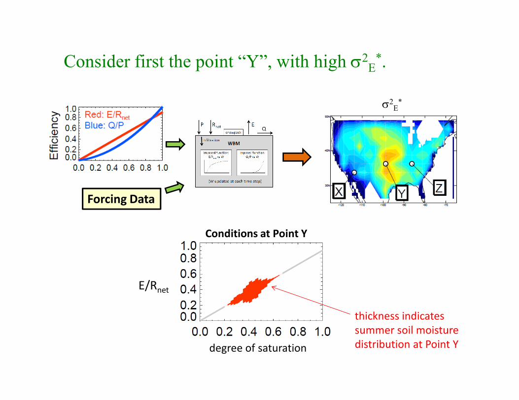
Consider first the point “Y”, with high σ2E*.
Forcing Data
σ2E*
Forcing Data
thickness indicates
summer soil moisture
distribution at Point Y
E/Rnet
degree of saturation
Conditions at Point Y

E/Rnet
degree of saturation
Conditions at Point Y σ2E*
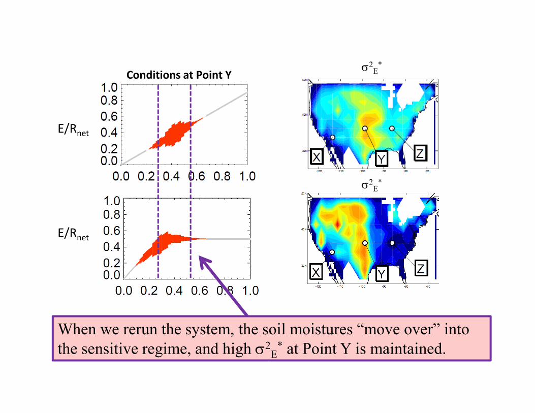
What happens if we rerun the system,
forcing the evaporation efficiency
curve to be flat at the soil moistures
characterizing Point Y?
E/Rnet
Conditions at Point Yσ2E
*
σ2E*
E/Rnet
When we rerun the system, the soil moistures “move over” into
the sensitive regime, and high σ2E* at Point Y is maintained.
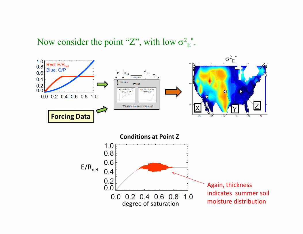
Now consider the point “Z”, with low σ2E*.
Forcing Data
σ2E*
Forcing Data
Again, thickness
indicates summer soil
moisture distribution
E/Rnet
degree of saturation
Conditions at Point Z
E/Rnet
degree of saturation
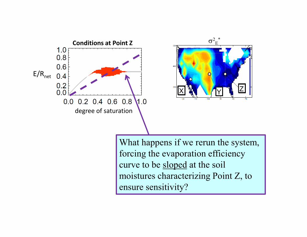
Conditions at Point Z σ2E*
What happens if we rerun the system,
forcing the evaporation efficiency
curve to be sloped at the soil
moistures characterizing Point Z, to
ensure sensitivity?
E/Rnet
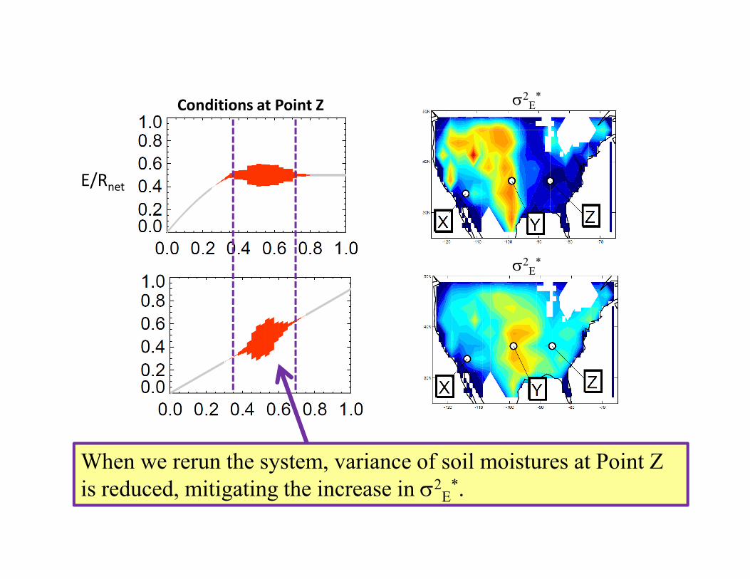
Conditions at Point Z σ2E*
σ2E*
When we rerun the system, variance of soil moistures at Point Z
is reduced, mitigating the increase in σ2E*.
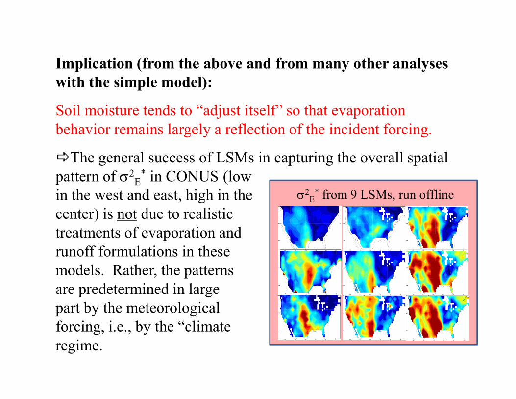
Implication (from the above and from many other analyses
with the simple model):
Soil moisture tends to “adjust itself” so that evaporation
behavior remains largely a reflection of the incident forcing.
The general success of LSMs in capturing the overall spatial
pattern of σ2E* in CONUS (low
in the west and east, high in the σ2E* from 9 LSMs, run offlinein the west and east, high in the
center) is not due to realistic
treatments of evaporation and
runoff formulations in these
models. Rather, the patterns
are predetermined in large
part by the meteorological
forcing, i.e., by the “climate
regime.
σ E from 9 LSMs, run offline
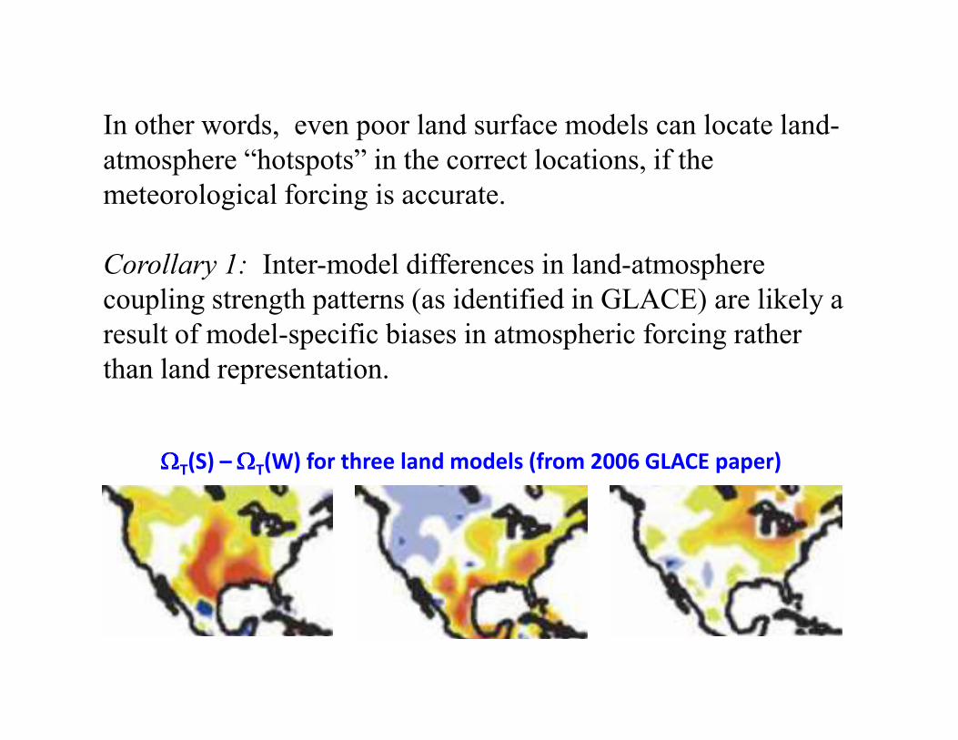
In other words, even poor land surface models can locate land-
atmosphere “hotspots” in the correct locations, if the
meteorological forcing is accurate.
Corollary 1: Inter-model differences in land-atmosphere
coupling strength patterns (as identified in GLACE) are likely a
result of model-specific biases in atmospheric forcing rather
than land representation.than land representation.
ΩΩΩΩT(S) – ΩΩΩΩT(W) for three land models (from 2006 GLACE paper)
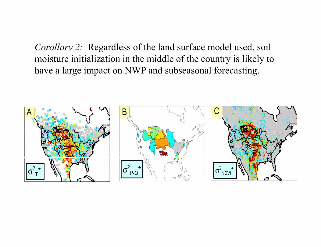
Corollary 2: Regardless of the land surface model used, soil
moisture initialization in the middle of the country is likely to
have a large impact on NWP and subseasonal forecasting.
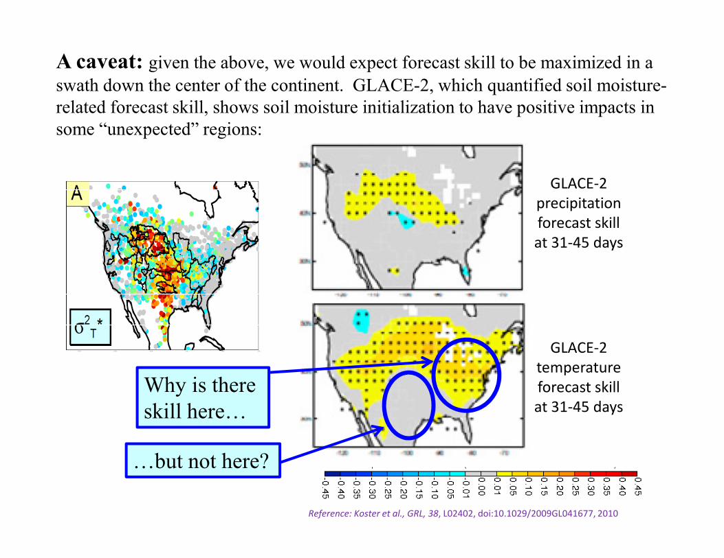
A caveat: given the above, we would expect forecast skill to be maximized in a swath down the center of the continent. GLACE-2, which quantified soil moisture-
related forecast skill, shows soil moisture initialization to have positive impacts in
some “unexpected” regions:
GLACE-2
precipitation
forecast skill
at 31-45 days
GLACE-2
temperature
forecast skill
at 31-45 days
Why is there
skill here…
…but not here?
Reference: Koster et al., GRL, 38, L02402, doi:10.1029/2009GL041677, 2010

The reasons for the apparent discrepancy are still unclear –
it’s an important question and a potentially fruitful topic of
future research.
For now, we can use a less scientific approach to explaining
things…
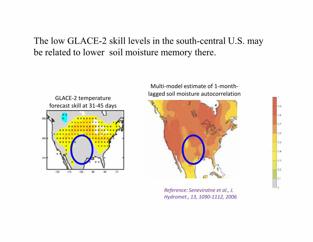
The low GLACE-2 skill levels in the south-central U.S. may
be related to lower soil moisture memory there.
GLACE-2 temperature
forecast skill at 31-45 days
Multi-model estimate of 1-month-
lagged soil moisture autocorrelation
Reference: Seneviratne et al., J.
Hydromet., 13, 1090-1112, 2006
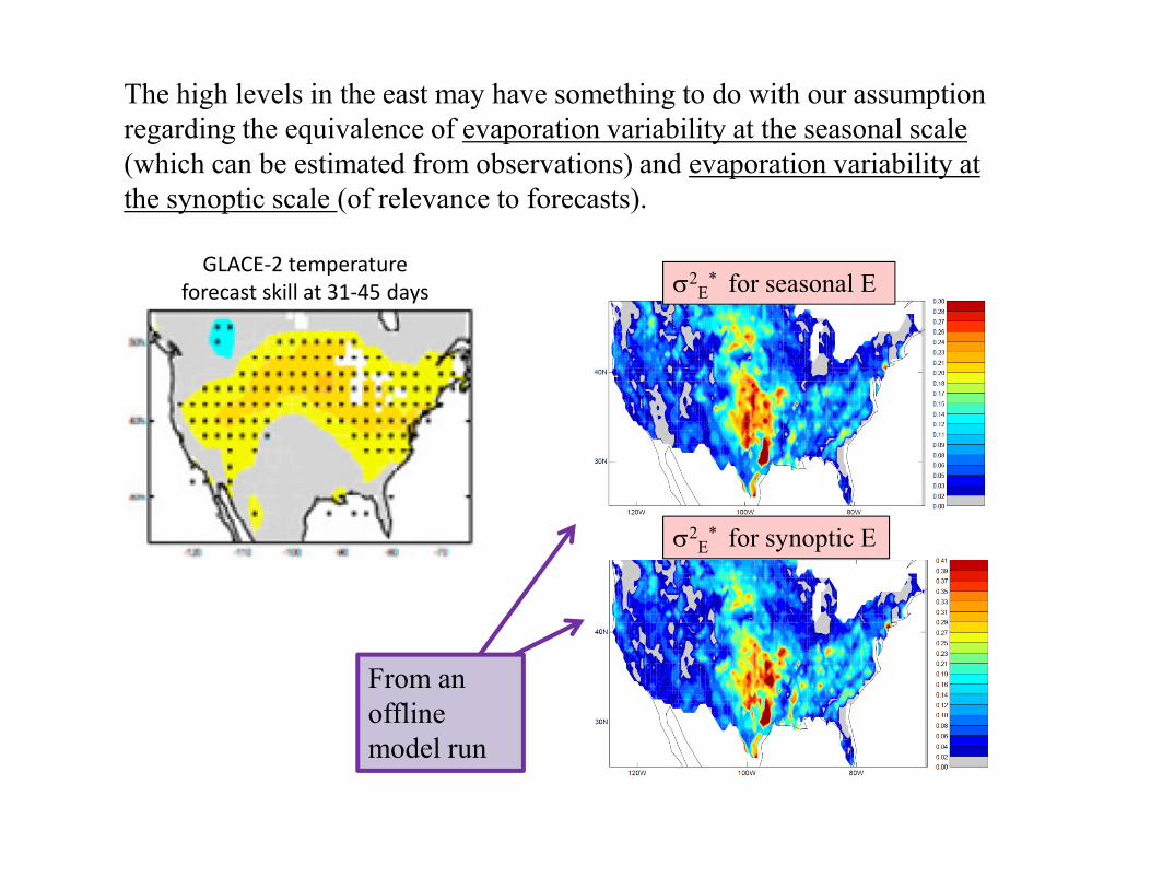
The high levels in the east may have something to do with our assumption
regarding the equivalence of evaporation variability at the seasonal scale
(which can be estimated from observations) and evaporation variability at
the synoptic scale (of relevance to forecasts).
σ2E* for seasonal E
GLACE-2 temperature
forecast skill at 31-45 days
σ2E* for synoptic E
From an
offline
model run
GLACE-2 temperature
forecast skill at 31-45 days σ2E* for seasonal E
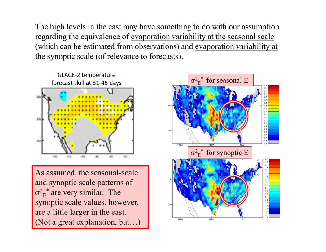
The high levels in the east may have something to do with our assumption
regarding the equivalence of evaporation variability at the seasonal scale
(which can be estimated from observations) and evaporation variability at
the synoptic scale (of relevance to forecasts).
σ2E* for synoptic E
As assumed, the seasonal-scale
and synoptic scale patterns of
σ2E* are very similar. The
synoptic scale values, however,
are a little larger in the east.
(Not a great explanation, but…)
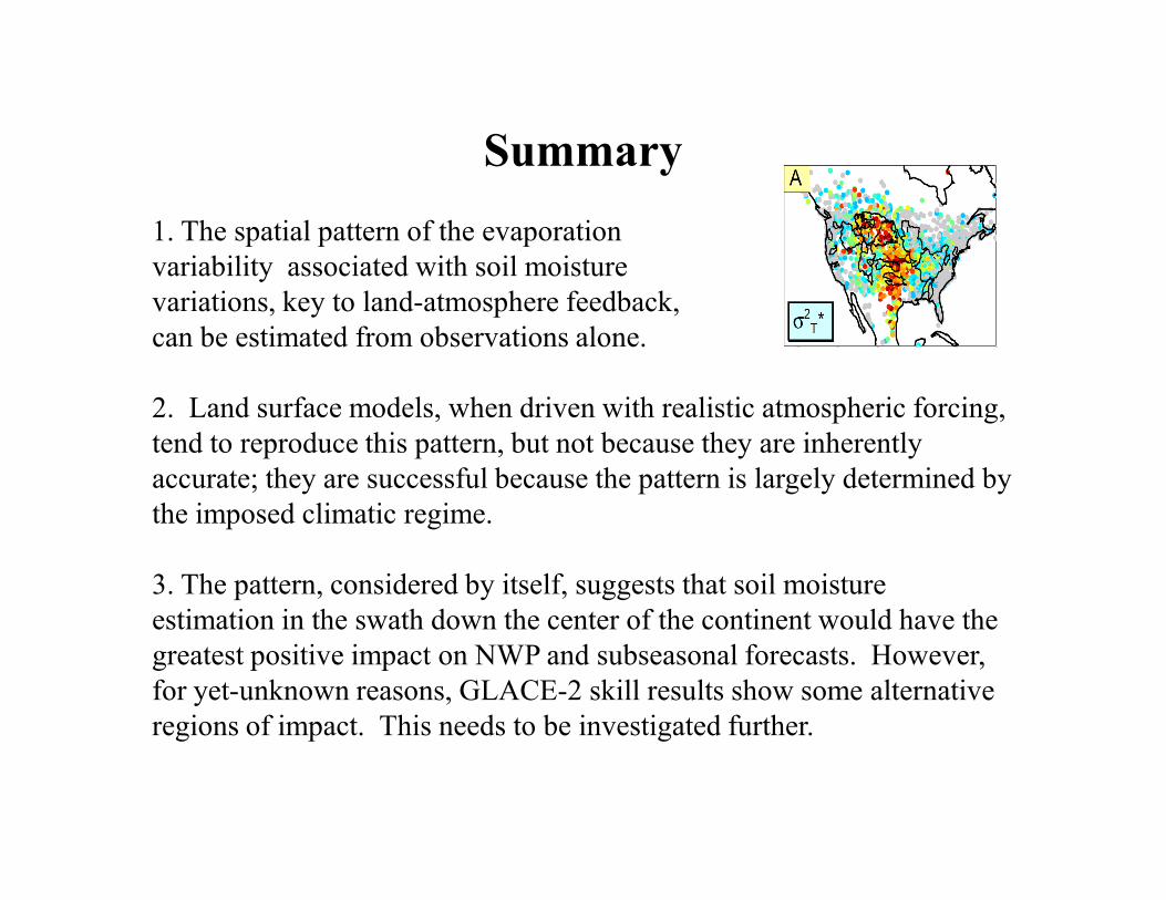
Summary
1. The spatial pattern of the evaporation
variability associated with soil moisture
variations, key to land-atmosphere feedback,
can be estimated from observations alone.
2. Land surface models, when driven with realistic atmospheric forcing,
tend to reproduce this pattern, but not because they are inherently tend to reproduce this pattern, but not because they are inherently
accurate; they are successful because the pattern is largely determined by
the imposed climatic regime.
3. The pattern, considered by itself, suggests that soil moisture
estimation in the swath down the center of the continent would have the
greatest positive impact on NWP and subseasonal forecasts. However,
for yet-unknown reasons, GLACE-2 skill results show some alternative
regions of impact. This needs to be investigated further.