arX

iv:1

201.

2963

v1 [

astr

o-ph

.IM]

13 J

an 2

012

Radio & Optical Interferometry:

Basic Observing Techniques and Data Analysis

To be published by Springer in Volume 2 of

Planets, Stars, & Stellar Systems

J.D. Monnier1 & R.J. Allen2

ABSTRACT

Astronomers usually need the highest angular resolution possible when observing

celestial objects, but the blurring effect of diffraction imposes a fundamental limit on

the image quality from any single telescope. Interferometry allows light collected at

widely-separated telescopes to be combined in order to synthesize an aperture much

larger than an individual telescope thereby improving angular resolution by orders of

magnitude. Because diffraction has the largest effect for long wavelengths, radio and

millimeter wave astronomers depend on interferometry to achieve image quality on

par with conventional large-aperture visible and infrared telescopes. Interferometers

at visible and infrared wavelengths extend angular resolution below the milli-arcsecond

level to open up unique research areas in imaging stellar surfaces and circumstellar

environments.

In this chapter the basic principles of interferometry are reviewed with an empha-

sis on the common features for radio and optical observing. While many techniques

are common to interferometers of all wavelengths, crucial differences are identified that

will help new practitioners to avoid unnecessary confusion and common pitfalls. The

concepts essential for writing observing proposals and for planning observations are de-

scribed, depending on the science wavelength, the angular resolution, and the field of

view required. Atmospheric and ionospheric turbulence degrades the longest-baseline

observations by significantly reducing the stability of interference fringes. Such insta-

bilities represent a persistent challenge, and the basic techniques of phase-referencing

and phase closure have been developed to deal with them. Synthesis imaging with large

observing datasets has become a routine and straightforward process at radio observa-

tories, but remains challenging for optical facilities. In this context the commonly-used

image reconstruction algorithms CLEAN and MEM are presented. Lastly, a concise

overview of current facilities is included as an appendix.

1monnier@umich.edu; Univ. Michigan Astronomy Dept., 941 Dennison Bldg, Ann Arbor, MI 48109-1090, USA.

2rjallen@stsci.edu; Space Telescope Science Institute, 3700 San Martin Drive, Baltimore, MD 21218, USA

– 2 –

1. Interferometry in Astronomy

1.1. Introduction

The technique of interferometry is an indispensable tool for modern astronomy. Typically

the telescope diameter D limits the angular resolution for an imaging system to Θ ≈ λD owing

to diffraction, but interferometry allows the achievement of angular resolutions Θ ≈ λB where the

baseline B is set by the distance between telescopes. Interferometry has permitted the angular

resolution at radio wavelengths to initially reach, and now to significantly surpass, the resolution

available with both ground- and space-based optical telescopes. Indeed, radio astronomers routinely

create high-quality images with high sensitivity, high angular resolution, and a large field-of-view

using arrays of telescopes such as the Very Large Array (VLA), the Combined Array for Research

in Millimeter-wave Astronomy (CARMA), and now the Atacama Large Millimeter Array (ALMA).

Interferometer arrays are now the instruments of choice for imaging the wide range of spatial

structures found both for Galactic and for extragalactic targets at radio wavelengths.

At optical wavelengths, interferometry can improve the angular resolution down to the milli-

arcsecond level, an order-of-magnitude better than even the Hubble Space Telescope. While at-

mospheric turbulence limits the sensitivity much more dramatically than for the radio, optical

interferometers can nevertheless measure the angular sizes of tens of thousands of nearby Galac-

tic objects and even a growing sample of distant Active Galactic Nuclei (AGN). Recently, optical

synthesis imaging of complex objects has been demonstrated with modern arrays of 4–6 telescopes,

producing exciting results and opening new avenues for research.

Both radio and optical interferometers also excel at precision astrometry, with the potential for

micro-arcsecond-level precision for some applications. Currently, it is ground-based radio interfer-

ometry (e.g. the VLBA) that provides the highest astrometric performance, although ground-based

near-IR interferometers are improving and measure different astronomical phenomena.

This chapter will provide an overview of interferometry theory and present some practical

guidelines for planning observations and for carrying out data analysis at the premier ground-

based radio and optical interferometer facilities currently available for research in astronomy. In

this chapter, the term “radio” will be used as a shorthand for the whole class of systems from sub-

mm to decametric wavelengths which usually employ coherent high-frequency signal amplification,

superheterodyne signal conversion, and digital signal processing, although detailed instrumentation

can vary substantially. Likewise, the term “optical” generally describes systems employing direct

detection, i.e. the direct combination of the signals from each collector without amplification or

mixing with locally-generated signals1.

1It should be emphasized, however, that this distinction is somewhat artificial; the first meter-wave radio interfer-

ometers ≈ 65 years ago were simple Michelson adding interferometers employing direct detection without coherent

high-frequency signal amplification. At the other extreme, superheterodyne systems are currently routinely used at

wavelengths as short as 10µm, such as the UC Berkeley ISI facility.

– 3 –

Historically, radio and optical interferometry have usually been discussed and reviewed in-

dependently from each other, leaving the student with the impression that there is something

fundamentally different between the two regimes of wavelength. Here a different approach is taken,

presenting a unified and more wavelength-independent view of interferometry, nonetheless noting

important practical differences along the way. This perspective will demystify some of the differing

terminology and techniques in a more natural way, and hopefully will be more approachable for a

broad readership seeking general knowledge. For a more much detailed treatment of radio interfer-

ometry specifically, refer to the classic text by Thompson et al. (2001) and the series of lectures in

the NRAO Summer School on Synthesis Imaging (e.g. Taylor et al. 1999). Optical interferometry

basics have been covered in individual reviews by Quirrenbach (2001) and by Monnier (2003), and a

useful collection of course notes can be found in the NASA-Michelson Course Notes (Lawson 2000)

and ESO-VLTI summer school proceedings (Malbet & Perrin 2007). Recently, a few textbooks have

been published on the topic of optical interferometry specifically, including Labeyrie et al. (2006),

Glindemann (2010), and Saha (2011). Further technical details can also be found in Chapters 7

and 13 of the first volume in this series.

This chapter begins with a brief history of interferometry and its scientific impact on as-

tronomy, a basic scientific context for newcomers that illustrates why the need for better angular

resolution has been and continues to be one of the most important drivers for technical innovation

in astronomy.

1.2. Scientific impact

Using interferometers in a synthesis imaging array allows designers to decouple the diffraction-

limited angular resolution of a telescope (which improves linearly with the telescope size) from its

collecting area (which, for a filled aperture, grows quadratically with the size). In the middle of the

20th century, radio astronomers faced a challenge in their new science; the newly-discovered “radio

stars” were bright enough to be observed with radio telescopes of modest collecting area, but the

resolution of conventional “filled aperture” reflecting telescopes was woefully inadequate (by one

or more orders of magnitude) to measure the positions and angular sizes of these enigmatic new

cosmological objects with a precision sufficient to permit an identification with an optical object.

Thus separated-element interferometry, although first applied in astronomy at optical wavelengths

(Michelson & Pease 1921), began to be applied in the radio with revolutionary results.

At radio wavelengths, the epoch of rapid technological development began more than 50 years

ago, and now interferometry is the “workhorse” technique of choice for most radio astronomers in

the world. A steady stream of exciting new results has flowed from these instruments even until

today, and a complete census of the major discoveries to date would be very lengthy indeed. Here,

our attention is focussed on the earliest historical discoveries that required radio interferometers,

and we have listed our nominations in Table 1. In Figure 1a, the spectacular image of radio jets

in quasar 3C175 by the VLA is shown to illustrate the high-fidelity imaging that is possible using

– 4 –

today’s radio facilities.

Modern long-baseline optical interferometry started approximately 30 years after radio inter-

ferometry, following the pioneering experiments and important scientific results with the Narrabri

intensity interferometry (e.g., Hanbury Brown et al. 1974) and the heterodyne work of the Townes’

group at Berkeley (Johnson et al. 1974). The first successful direct interference of stellar light

beams from separated telescopes was achieved in 1974 (Labeyrie 1975) and this was followed by

about twenty years of two-telescope (i.e., single baseline) experiments which measured the angu-

lar diameters of a variety of objects for the first time. The first imaging arrays with more than

two telescopes were constructed in the 1990s, and the COAST interferometer was first to make a

true optical synthesis image using techniques familiar to radio astronomers (Baldwin et al. 1996).

Keck and VLT interferometers both include 8-m class telescopes, making them the most sensitive

facilities in the world. Recently, the CHARA array has produced a large number of new images in

the infrared using combinations of 4 telescopes simultaneously. Table 1 lists a few major scientific

accomplishments in the history of optical interferometry showing the diversity of contributions in

many areas of stellar astronomy and even recent extragalactic observations of active galactic nuclei.

With technical and algorithm advances, model-independent imaging has become more powerful and

a state-of-the-art image from the CHARA array is presented in Figure 1b, showing the surface of

the rapidly rotating star Alderamin.

2. Interferometry in theory and practice

2.1. Introduction

The most basic interferometer used in observational astronomy consists of two telescopes con-

figured to observe the same object and connected together as a Michelson interferometer. Photons

collected at each telescope are brought together to a central location and combined coherently

at the “correlator” (radio term) or the “combiner” (optical term). For wavelengths longer than

∼0.2 millimeters, the free-space electric field is usually converted into cabled electrical signals and

coherently amplified at the focus of each telescope. The celestial signal is then mixed with a lo-

cal oscillator signal sent to both telescopes from a central location, and the difference frequency

transmitted in cables back to the centrally-located correlator. For shorter wavelengths, cable losses

increase, and signal transmission moves eventually into free space in a more ”optical” mode, using

mirrors and long-distance transmission of light beams in (sometimes evacuated) pipes.

Depending on the geometry, the light from an astronomical object will in general be received

at one telescope before it arrives at the other. If the fractional signal bandwidth ∆ν is very narrow

(either because of the intrinsic emission properties of the source, e.g. a spectral line, or because

of imposed bandwidth limitations in amplifiers and/or filters), then the signal has a high degree

of “temporal coherence”, which is to say that the wave packet describing all the photons in the

signal is extended in time by τ ≈ 1/∆ν seconds. Expressing the bandwidth in terms of wavelength,

– 5 –

Table 1. Some historically-important astronomical results made possible by interferometry

Astronomical Result Date Facility Referencesa

Radio Interferometryb

Solar radio emission from sunspots 1945-46 Australia, Sea cliff interferometer R1

First Radio Galaxies NGC 4486 & NGC 5128 1948 New Zealand, Sea cliff interferometer R2

Identification of Cygnus A 1951-53 Cambridge, Wurzburg antennas R3

Cygnus A double structure 1953 Jodrell Bank, Intensity interferometer R4

AGN superluminal motions 1971 Haystack-Goldstone VLBI R5

Dark matter in spiral galaxies 1972-78 Caltech interferometer, Westerbork SRT R6

Spiral arm structure & kinematics 1973-80 Westerbork SRT R7

Compact source in Galactic center 1974 NRAO Interferometer R8

Gravitational lenses 1979 Jodrell Bank Mk1 + Mk2 VLBI R9

NGC 4258 black hole 1995 NRAO VLBA R10

Optical Interferometry

Physical diameters of hot stars 1974 Narrabri Intensity Interferometer O1

Empirical effective temperature scale for giants 1987 I2T/CERGA O2

Survey of IR Dust Shells 1994 ISI O3

Geometry of Be star disks 1997 Mark III O4

Near-IR Sizes of YSO disks 2001 IOTA O5

Pulsating Cepheid ζ Gem 2001 PTI O6

Crystalline silicates in inner YSO disks 2004 VLTI O7

Vega is a rapid rotator 2006 NPOI O8

Imaging gravity-darkening on Altair 2007 CHARA O9

Near-IR sizes of AGN 2009 Keck-I O10

aReferences: R1: Pawsey et al. (1946); McCready et al. (1947). R2: Bolton et al. (1949). R3: Smith (1951);

Baade & Minkowski (1954). R4: Jennison & Das Gupta (1953). R5: Whitney et al. (1971); Cohen et al. (1971).

R6: Rogstad & Shostak (1972); Bosma (1981a,b). R7: Allen et al. (1973); Rots & Shane (1975); Rots (1975); Visser

(1980b,a). R8: Goss et al. (2003). R9: Porcas et al. (1979); Walsh et al. (1979). R10: Miyoshi et al. (1995).

O1: Hanbury Brown et al. (1974). O2: di Benedetto & Rabbia (1987). O3: Danchi et al. (1994). O4: Quirrenbach et al.

(1997). O5: Millan-Gabet et al. (2001). O6: Lane et al. (2000). O7: van Boekel et al. (2004). O8: Peterson et al.

(2006). O9: Monnier et al. (2007). O10: Kishimoto et al. (2009).

bRadio list in part from Wilkinson et al. (2004) and R.D. Ekers (2010, priv. comm.), with additions by one of the

authors (RJA). Historical material prior to 1954 is also from W.M. Goss (2011, private communication) and Sullivan

(2009).

– 6 –

∆ν = (c/λ20) · ∆λ where λ0 is the band center and c is the speed of light. The coherence time is

then τ = (1/c) · (λ20/∆λ), and c · τ is a scale size of the wave packet called the coherence length,

Lc = c·τ = λ20/∆λ, (e.g. Hecht 2002, Ch. 7). If the path difference between the two collectors in an

interferometer is a significant fraction of Lc, an additional time delay must be introduced, otherwise

the fringe amplitude will decrease or even disappear. For ground-based systems, the geometry is

continually changing for all directions in the sky (except in the directions to the equatorial poles),

requiring a continually-changing additional delay to maintain the temporal coherence. The special

location on the sky where the adjusted time delay is matched perfectly is often called the “phase

center” or point of zero optical path delay (OPD), although such a condition actually defines the

locus of a plane passing through the mid-point between the collectors and perpendicular to the

baseline, and cutting the celestial sphere in a great circle. Since the telescope optics usually limits

the field of view to only a tiny portion of this great circle, adjusting the phase center is the equivalent

of “pointing” the interferometer at a given object within that field of view.

The final step is to interfere the two beams to measure the spatial coherence (often called the

mutual coherence) of the electric field as sampled by the two telescopes. If the object observed is

much smaller than the angular resolution of the interferometer, then interference is complete and

one observes 100% coherence at the correlator/combiner. However, objects that are resolved (i.e.,

much larger than the angular resolution of the interferometer) will show less coherence due to the

fact that different patches of emission on the object do not interfere at the same time through our

system. Figure 2 shows two simple cases of an interferometer as a Young’s two-slit experiment to

illustrate basic principles. At the left, the interferometer is made up of two slits and the response for

a monochromatic point source (i.e., incoming plane waves) is shown. The result should be familiar:

an interference fringe modulating the intensity from 100% to 0% with a periodicity that corresponds

to a fringe spacing of λB on the sky. Next to this panel is shown an example of two equal-brightness

point sources separated by 12λB , half the fringe spacing. The location of constructive interference

for one point coincides with the location of destructive interference for the other source. Since the

two sources are mutually incoherent, the superposition of the two fringe results in an even light

distribution, i.e. no fringe at all! In optical interferometry language, the first example fringe has a

fringe contrast (or visibility) of 1 while the second example fringe has a visibility of 0.

Figure 3 contains a schematic of a basic interferometer as typically realized for both radio

and optical configurations. While instrumental details vary immensely in how one transmits and

interferes the signals for radio, millimeter, infrared, and visible-light interferometers, the basic

principles are the same. The foundational theory common to all interferometers will be introduced

next.

2.2. Interferometry in theory

The fundamental equation of interferometry is typically derived by introducing the van-Cittert

Zernike Theorem and a complete treatment can be found in Chapter 3 of the book by Thompson et al.

– 7 –

(2001). Here the main result will be presented without proof, beginning by defining an interfero-

metric observable called the complex visibility, V. The visibility can be derived from the intensity

distribution on the sky I(~σ) using a given interferometer baseline ~B (which is the separation vector

between two telescopes) and the observing wavelength λ:

V = |V|eiφV =

∫

skyAN (~σ)I(~σ)e−

2πiλ

~B·~σdΩ (1)

Here, the ~σ represents the vector pointing from the center of the field-of-view (called the “phase

center”) to a given location on the celestial sphere using local (East, North) equatorial coordinates

and the telescope separation vector ~B also using east and north coordinates. The modulus of the

complex visibility |V| is referred to as the fringe amplitude or visibility while the argument φV is

the fringe phase. AN (~σ) represents the normalized pattern that quantifies how off-axis signals are

attenuated as they are received by a given antenna or telescope. In this treatment the astronomical

object is assumed to be small in angular size in order to ignore the curvature of the celestial sphere.

The physical baseline ~B can be decomposed into components ~u = (u, v) in units of observing

wavelength along the east and north directions (respectively) as projected in the direction of our

target. The vector ~σ = (l,m) also can be represented in rectilinear coordinates on the celestial

sphere, where l points along local east and m points north2. Here, l and m both have units of

radians. Equation 1 now becomes:

V(u, v) = |V|eiφV =

∫

l,mAN (l,m)I(l,m)e−2πi(ul+vm)dldm (2)

The fundamental insight from Equation 2 is that an interferometer is a Fourier Transform machine

– it converts an intensity distribution I(l,m) into measurements of Fourier components V(u, v) forall the baselines in the array represented by the (u, v) coverage. Since an intensity distribution

can be described fully in either image space or Fourier space, the collection of sufficient Fourier

components using interferometry allows for an image reconstruction through an inverse Fourier

Transform process, although practical limitations lead to compromises in the quality of such images.

2.3. Interferometry in practice

In this section, the similarities and differences between radio and optical interferometers are

summarized along with the reasons for the main differences. Interested readers can find more

detailed on specific hardware implementations in Volume I of this series.

Modern radio and optical interferometers typically use conventional steerable telescopes to

collect photons from the target. In the radio, a telescope is often called an antenna; it is typically

2There are several different coordinate systems in use to describe the geometry of ground-based interferometers

used in observing the celestial sphere; (see e.g. Thompson et al. 2001, Chapter 4 and Appendix 4.1).

– 8 –

a parabolic reflector with a very short focal length (f/D ≈ 0.35 is common), with signal collection

and initial amplification electronics located at the prime focus. Owing to the large value of ∆Θ ∼λ

Diameter , the diffraction pattern of the antenna aperture is physically a relatively large region at

the prime focus. This fact, coupled with the cost and complexity of duplicating and operating

many low-noise receivers in close proximity to each other, has meant that antennas used in radio

astronomy typically have only a “single-pixel” signal collection system (a dipole or a “feed horn”)

at the prime focus3. Light arriving from various directions on the sky are attenuated depending

on the shape of the diffraction pattern, written as AN in Equation 2 and often called the “antenna

pattern” or the “primary beam”. The signal collection system may be further limited to a single

polarization mode, although systems are common that simultaneously accept both linear (or both

circular) polarization states. After initial amplification, the signal is usually mixed with a local

oscillator to “down-convert” the high frequencies to lower frequencies that can more easily be

amplified and processed further. These lower-frequency signals from the separate telescopes can

also be more easily transported over large distances to a common location using e.g. coaxial cable, or

by modulating an optical laser and using fiber optics. This common location houses the “back end”

of the receiver, where the final steps in signal analysis are carried out including band definition,

correlation, digitizing, and spectral analysis. In some cases, the telescope signals are recorded

onto magnetic media and correlated at a later time and in a distant location (e.g. the “Very Long

Baseline Array” or global VLBI).

In the optical, the light from the object is generally focused by the telescope, re-collimated into

a compressed beam for free-space transport, and then sent to a central location in a pipe which is

typically evacuated to avoid introducing extra air dispersion and ground-level turbulence. In rare

cases, the light at the telescope is focused directly into a single-mode fiber, which is the dielectric

equivalent to the metallic waveguides used in radio and millimeter receivers. Note that atmospheric

seeing is very problematic for even small visible and infrared telescopes while it is usually negligible

compared to the diffraction limit for even the largest radio and mm-wave telescopes.

Both radio and optical interferometers must delay the signals from some telescopes to match

the optical paths. After mixing to a lower frequency, radio interferometers can use switchable

lengths of coaxial cable in order to introduce delays. More recently, the electric fields can be

directly digitized with bandwidths of > 5 GHz, and these “bits” can be saved in physical memory

and then recalled at a later time. For visible and infrared systems, switchable fiber optics are not

practical due to losses and glass dispersion; the only solution is to use an optical “free-space” delay

line consisting of a retroreflector moving on a long track and stabilized through laser metrology to

compensate for air path disturbances and vibrations in the building.

In a radio interferometer, once all the appropriate delays have been introduced the signals

from each telescope can be combined. Early radio signal correlators operated in an “optical” mode

3Very recently, several radio observatories have begun to equip their antennas (and at least one entire synthesis

telescope) with arrays of such feeds.

– 9 –

as simple adding interferometers, running the sum of the signals from the two arms through a

square-law detector. The output of such a detector contains the product of the two signals. Unfor-

tunately, the desired correlation product also comes with a large total power component caused by

temporally-uncorrelated noise photons contributed (primarily) by the front-end amplifiers in each

arm of the interferometer plus atmosphere and ground noise. This large signal demanded excellent

DC stability in the subsequent electronics, and it was not long in the history of radio interferome-

try before engineers found clever switching and signal-combination techniques to suppress the DC

component. These days signal combiners deliver only the product of the signals from each arm, and

are usually called “correlators”4. Most modern radio/millimeter arrays use digital correlators that

introduce time lags between all pairs of telescopes in order to do a full temporal cross-correlation.

This allows a detailed wavelength-dependent visibility to be measured, i.e., an interferometric spec-

trum with R = λ∆λ > 100000 if necessary. By most metrics, radio correlators have reached their

fundamental limit in terms of extracting full spectral and spatial information and can be fairly

sophisticated and complex to configure when correlating multiple bandpasses simultaneously with

high spectral resolution5.

In the visible and infrared, the electric fields can not be further amplified without strongly

degrading the signal-to-noise ratio, and so parsimonious beam combining strategies are common

that split the signal using e.g. partly-reflecting mirrors into a small number of pairs or triplets.

Furthermore, most optical systems have only modest spectral resolutions of typically R ∼ 40

in order to maintain high signal-to-noise ratio, although a few specialized instruments exist that

reach R > 1000 or even R > 30000. Signal combination finally takes place simply by mixing the

light beams together and modulating the relative optical path difference, either using spatial or

temporal encoding. The total power measurement in a visible-light or infrared detector will reveal

the interference fringe and a Fourier analysis can be used to extract the complex visibility V.

Because the ways of measuring visibilities are quite different, radio and optical interferometrists

typically report results in different units. Radio/mm interferometers measure correlated flux density

in units of Jansky (10−26 W m−2 Hz−1), just as suggested by Equation 26. In the optical however,

interferometers tend to always measure a normalized visibility that varies from 0 to 1 – this is

simply the correlated signal normalized by the total power. One can convert the latter to correlated

4This is not all advantageous; if the data is intended to be used in an imaging synthesis, the absence of the total

power component means that the value of the map made from the data will integrate to zero. In other words, without

further processing the image will be sitting on a slightly-negative “floor”. If more interferometer spacings around

zero are also missing, the floor becomes a “bowl”. All this is colloquially called “the short-spacing problem”, and

it adversely affects the photometric accuracy of the image. A significant part of the computer processing “bag of

tricks” used to “restore” such images is intended to address this problem, although the only proper way to do that

is to obtain the missing data and incorporate it into the synthesis.

5At millimeter and sub-millimeter wavelengths, correlators still do not attain the maximum useful bandwidths for

continuum observations

6Recall that an integration of specific intensity over solid angle results in a flux density, often expressed in Jansky.

– 10 –

flux density by simply multiplying by the known total flux density of the target at the observed

wavelengths, or otherwise by carrying out a calibration of the system by a target of known flux

density.

2.3.1. Quantum limits of amplifiers

The primary reason why radio and optical interferometers differ so much in their detection

scheme is because coherent amplifiers would introduce too much extraneous noise at the high

frequencies encountered in the optical and infrared. This difference is fundamental and is explored

in more detail in this section.

At radio frequencies there are huge numbers of photons in a typical sample of the electromag-

netic field, so the net phase of a packet of radio photons (either from the source or from a noisy

receiver) is well-defined and amplifiers can operate coherently. The ultimate limits which apply to

such amplifiers are dictated by the uncertainty principle as stated by Heisenberg. Beginning with

the basic “position - uncertainty” relation ∆x ∆px ≥ h/4π, it is easy to derive the “energy - time”

relation ∆E ∆t ≥ h/4π. Since the uncertainty in the energy of the n photons in a wave packet can

be written as ∆E = hν ∆n and the uncertainty in the phase of the aggregate as ∆φ = 2πν ∆t,

this leads to the equivalent uncertainty relation ∆φ ∆n ≥ 1/2.

An ideal amplifier which adds no noise to the input photon stream leads to a contradiction of

the uncertainty principle. The following argument shows how this happens (adapted from Heffner

1962): Consider an ideal coherent amplifier of gain G which creates new photons in phase coherence

with the input photons, and assume it adds no incoherent photons of its own to the output photon

stream. With n1 photons going into such an amplifier, there will be n2 = Gn1 photons at the

output, all with the same phase uncertainty ∆φ2 = ∆φ1 with which they went in. In addition, in

this model it is expected that ∆n2 = G∆n1 (no additional “noise” photons unrelated to the signal).

But according to the same uncertainty relation, the photon stream coming out of the amplifier must

also satisfy ∆φ2 ∆n2 ≥ 1/2. This would imply that ∆φ1 ∆n1 ≥ 12G , which for large G says that

the input photon number and wave packet phase could be measured with essentially no noise.

But this contradicts the same uncertainty relation for the input photon stream, which requires that

∆φ1 ∆n1 ≥ 1/2. This contradiction shows that one or more of our assumptions must be wrong. The

argument can be saved if the amplifier itself is required to add noise of its own to the photon stream;

the following heuristic construction shows how. Using the identity ∆n2 = (G−N) ·∆n1 +N∆n1at the output (where N is an integer N ≥ 1), and referring this noise power back to the input by

dividing it with the amplifier gain G, this leads to (1−N/G) ·∆n1 + (N/G) ·∆n1 at the input to

the amplifier, which for large G is ∆n1. The smallest possible value of N is 1. This preserves the

uncertainty relation at the expense of an added minimum noise power of hν at the input. Oliver

(1965) has elaborated and generalized this argument to include all wavelength regimes, and has

shown that the minimum total noise power spectral density ψν of an ideal amplifier (relative to the

– 11 –

input) is

ψν =hν

e(hν/kT ) − 1+ hν Watts/Hz , (3)

where T is the kinetic temperature that the amplifier input faces in the propagation mode to

which the amplifier is sensitive. For hν < kT this reduces to ψν ≈ kT Watts/Hz, which can be

called the ”thermal” regime of radio astronomy. For hν > kT this becomes ψν ≈ hν Watts/Hz

in the ”quantum” regime of optical astronomy. The crossover point where the two contributions

are equal is where hν/kT = ln 2, or at λc · Tc = 20.75 (mm K). As an illustration of the use of

this equation, consider this example: The sensitivity of high-gain radio-frequency amplifiers can

usually be improved by reducing their thermodynamic temperatures. However, for instance at a

wavelength of 1 mm, it might be unnecessary (depending on details of the signal chain) to aim for

a high-gain amplifier design to lower the thermodynamic temperature below about 20K, since at

that point the sensitivity is in any case limited by quantum noise. At even shorter wavelengths,

the rationale for cooled amplifiers disappears, and at optical wavelengths amplifiers are clearly not

useful since the noise is totally dominated by spontaneous emission7 and is equivalent to thermal

emission temperatures of thousands of degrees. The extremely faint signals common in modern

optical observational astronomy translate into very low photon rates, and the addition of such

irrelevant photons into the data stream by an amplifier would not be helpful.

2.4. Atmospheric Turbulence

So far, the analysis of interferometer performance has assumed a perfect atmosphere. However,

the electromagnetic signals from cosmic sources are distorted as they pass through the intervening

media on the way to the telescopes. These distortions occur first in the interstellar medium,

followed by the interplanetary medium in the solar system, then the Earth’s ionosphere, and finally

the Earth’s lower atmosphere (the troposphere) extending from an altitude of ≈ 11 km down to

ground level. The media involved in the first three sources of distortion contain ionized gas and

magnetic fields, and their effects on signal propagation depend strongly on wavelength (generally

as ∝ λ2) and polarization. At wavelengths shorter than about 10 cm the troposphere begins to

dominate. Molecules in the troposphere (especially water vapor) become increasingly troublesome

at frequencies above 30 GHz (1 cm wavelength), and the atmosphere is essentially opaque beyond

300 GHz except for two rather narrow (and not very clear) “windows” from 650-700 and 800-900

GHz which are usable only at the highest-altitude sites. The next atmospheric windows appear in

the IR at wavelengths less than about 15 microns. The optical window opens around one micron,

and closes again for wavelengths shorter than about 350 nm.

The behavior of the troposphere is thus of prime importance to ground-based astronomy at

7Although amplifiers are currently used in the long-distance transmission of near-IR (digital) communication

signals in optical fibers, the signal levels are relatively large and low noise is not an important requirement.

– 12 –

wavelengths from the decimeter-radio to the optical. Interferometers are used in the study of

structure in the troposphere, and a summary of approaches and results with many additional

references is given in Thompson et al. (2001); Carilli & Holdaway (1999); Sutton & Hueckstaedt

(1996, Ch. 13). A discussion oriented towards optical wavelengths can be found in Quirrenbach

(2000). Since the main focus here is on using interferometers to measure the properties of the

cosmic sources themselves, our discussion is limited to some “rules of thumb” for choosing the

interferometer baseline length and the time interval between measurements of the source and of a

calibrator in order to minimize the deleterious effects of propagation on the fringe amplitudes and

(especially) fringe phases.

2.4.1. Phase fluctuations – length scale

Owing to random changes in the refractive index of the atmosphere and the size distribution

of these inhomogeneities, the path length for photons will be different along different parallel lines

of sight. This fluctuating path length difference grows almost linearly with the separation d of the

two lines of sight for separations up to some maximum, called the outer scale length (typically tens

to hundreds of meters, with some weak wavelength dependence), and is roughly constant beyond

that. Surprisingly, in spite of the differences in the underlying physical processes causing refraction,

variations in the index of refraction are quite smooth across the visible and all the way through to

the radio. At short radio wavelengths, the fluctuations are dominated by turbulence in the water

vapor content; at optical/IR wavelengths, it is temperature and density fluctuations in dry air that

dominate.

Using a model of fully-developed isotropic Kolmogorov turbulence for the Earth’s atmo-

sphere, the rms path length difference grows according to σd ∝ d5/6 for a path separation d (see

Thompson et al. 2001, Ch. 13, for references). High altitude sites show smaller path length dif-

ferences as the remaining vertical thickness of the water vapor layer decreases. Relatively large

seasonal and diurnal variations also exist at high mountain sites as the atmospheric temperature

inversion layer generally rises during the summer and further peaks during mid-day. Variations in

σd by factors of ∼ 10 are not unusual (see Thompson et al. 2001, Fig. 13.13), but a rough average

value for a good observing site is σd ≈ 1 mm for baselines d ≈ 1 km at millimeter wavelengths, and

σd ≈ 1 micron for baselines d ≈ 50 cm at infrared wavelengths.

The length scale fluctuations translate into fringe phase fluctuations of σφ = 2πσd/λ in radians.

The maximum coherent baseline d0 is defined as that baseline length for which the rms phase

fluctuations reach 1 radian. Using the expressions in the previous paragraph and coefficients suitable

for the radio and optical ranges at the better observing sites, two useful approximations are d0 ≈140 · λ6/5 meters for λ in millimeters (useful at millimeter radio wavelengths), and d0 ≈ 10 ·λ6/5 centimeters for λ in microns (useful at IR wavelengths). These two expressions are in fact

quite similar; using the “millimeter expression” to calculate d0 in the IR underestimates the value

obtained from the “IR expression” by a factor of 2.8, which is at the level of precision to be expected.

– 13 –

At shorter wavelengths (visible and near-infrared), atmospheric turbulence limits even the

image quality of small telescopes. This has led to a slightly different perspective for the length scale

that characterizes atmospheric turbulence, although it is closely related to the previous description.

The Fried length r0 (Fried 1965) is the equivalent-sized telescope diameter whose diffraction limit

matches the image quality through the atmosphere due to seeing. It turns out that this quantity

is proportional to the length scale where the rms phase error over the telescope aperture is ≈ 1

radian. In other words, apertures with diameters small compared to r0 are approximately diffraction

limited, while larger apertures have resolution limited by turbulence to ≈ λ/r0. It can be shown

that, for an atmosphere with fully-developed Kolmogorov turbulence, r0 ≈ 3.2d0 (Thompson et al.

2001, Ch. 13).

2.4.2. Phase fluctuations – time scale

Although fluctuations of order one radian may be no more than a nuisance at centimeter

wavelengths, requiring occasional phase calibration (see §3.1.3), they will be devastating at IR

and visible wavelengths owing to their rapid variations in time. In order to relate the temporal

behavior of the turbulence to its spatial structure, a model of the latter is required along with

some assumption for how that structure moves over the surface of the Earth. One specific set

of assumptions is described in Thompson et al. (2001, Ch. 13); however, for the purposes here

it is sufficient to use Taylor’s “frozen atmosphere” model with a nominally-static phase screen

that moves across the Earth’s surface with the wind at speed vs. This phase screen traverses the

interferometer baseline d in a time τd = d/vs, at the conclusion of which the total path length

variation is σd. Taking the critical time scale τc to be when the rms phase error reaches 1 radian,

then τc ≈ d0/vs with d0 given in the previous paragraph. As an example consider a wind speed

of 10 m/s; this leads to τc ≈ 14 seconds at λ = 1 mm, and ≈ 10 milliseconds at λ = 1 micron.

Clearly the techniques required to manage these variations will be very different at the two different

wavelength regimes, even though the magnitude of the path length fluctuations (in radians of phase)

are similar. Representative values of these quantities are collected in Table 2.

2.4.3. Calibration – Isoplanatic Angle

The routine calibration of interferometer phase and amplitude is usually done by observing

a source with known position and intensity inter-leaved in time with the target of interest. At

centimeter wavelengths and longer, the discussion in the previous section indicates that such mea-

surements can be done on time scales of minutes to hours, providing ample time to re-position

telescopes elsewhere on the sky in order to observe a calibrator. But how close to the target of

interest does such a calibrator have to be? Ideally, the calibrator ought to be sufficiently nearby on

the celestial sphere that the line of sight traverses a part of the atmosphere with substantially the

same phase delay as the line of sight to the target. This angle is called the isoplanatic angle Θiso;

– 14 –

it characterizes the angular scale size over which different parts of the incoming wavefront from the

target encounter closely similar phase shifts, thereby minimizing the image distortion. The isopla-

natic angle can be roughly estimated by calculating the angle subtended by an r0-sized patch at a

height h that is characteristic for the main source of turbulence; hence, roughly Θiso ≈ r0h . Within a

patch on the sky with this angle, the telescope/interferometer PSF remains substantially constant,

retaining the convolution relation between the source brightness distribution and the image. Some

approximate values are given in Table 2 as a guide.

At visible and near-IR wavelengths, Table 2 shows that the isoplanatic angle is very small,

smaller than an arcminute. Unfortunately, the chance of having a suitably bright and point-like

object within this small patch of the sky is very low. Even if an object did exist, it would be nearly

impossible to repetitively re-position the telescope and delay line at the milli-second level timescale

needed to “freeze” the turbulence between target and calibrator measurements. Special techniques

to deal with this problem will be discussed further in section 3.1.3.

3. Planning Interferometer Observations

The issues to consider when writing an interferometer observing proposal or planning the

observations themselves include: the desired sensitivity (i.e., the unit telescope collecting area, the

number of telescopes to combine at once, the amount of observing time), the required field-of-view

and angular resolution (i.e.,the shortest and longest baselines), calibration strategy and expected

systematic errors (i.e., choosing phase and amplitude calibrators), the expected complexity in the

image (i.e., the completeness of u,v coverage, do science goals demand model-fitting or model-

independent imaging), and the spectral resolution (i.e., correlator settings, choice of combiner

instrument). Many of these issues are intertwined, and the burden on the aspiring observer to

reach a compatible set of parameters can be considerable. Prospective observers planning to use

the VLA are fortunate to have a wide variety of software planning tools and user’s guides already

at their disposal, but those hoping to use more experimental facilities or equipment which is still

in the early phases of commissioning will find their task more challenging.

Here, the most common issues encountered during interferometer observations will be intro-

duced. In many ways this is more of a list of things to worry about rather than a compendium

of solutions. The basic equations and considerations have been collected in Table 3. In order to

obtain the latest advice on optimizing a request for observing time, or to plan an observing run,

observers ought to consult the web sites, software tools, and human assistants available for them

at each installation (see Appendix for a list of current facilities).

– 15 –

Table 2. Approximate baseline length, Fried length, and time scales for a 1-radian rms phase

fluctuation in the Earth’s troposphere and a wind speed of 10 m/s.a

Max. Coherent Fried length Time scale Isoplanatic angle at zenith

Wavelength Baseline d0 r0 τc Θiso

0.5 µm (visible) 4.4 cm 14 cm 4.4 ms 5.5′′

2.2 µm (near-IR) 26 cm 83 cm 26 ms 33′′

1 mm (millimeter) 140 m 450 m 14 sec 3.5

10 cm (radio) 35 km 112 km 58 min largeb

a From parameters for Kolmogorov turbulence given in Thompson et al. (2001, Ch. 13), and in Woolf

(1982, Table 2). The inner and outer scale lengths are presumed to remain constant in these rough

approximations. Values are appropriate for a good observing site and improve at higher altitudes. See

§2.4 for more discussion.

b Limited in practice by observing constraints such as telescope slew rates and elevation limits, and

source availability.

Table 3. Planning Interferometer Observations

Consideration Equation

Angular Resolution Θ = 1

2

λBmax

Spectral Resolution R = λ∆λ

= c∆v

Field-of-View

primary beam ∆Θ ∼ λDTelescope

bandwidth-smearing ∆Θ ∼ R · λBmax

time-smearing ∆Θ ∼ 230

∆tminutes

λBmax

Phase Referencing

Coherence Time see Table 2

Isoplanatic Angle see Table 2

– 16 –

3.1. Sensitivity

Fortunately modern astronomers can find detailed documentation on the expected sensitivities

for most radio and optical interferometers currently available. Indeed, the flexibility of modern

instrumentation sometimes defies a back-of-the-envelope estimation for the true signal-to-noise

ratio (SNR) expected for a given observation. In order to better understand what limits sensitivity

for real systems, the dominant noise sources and the key parameters affecting signal strength are

introduced. Most of the focus will be for observations of point sources since resolved sources do

not contribute signal to all baselines in an array and this case must be treated with some care.

Here, the discussions of the radio and optical cases are separate because of the large differences

in the nature of the noise processes (e.g., see §2.3.1) and the associated nomenclature. Radio and

optical observations lie at the two limits of Bose-Einstein quantum statistics that govern photon

arrival rates (e.g., Pathria 1972, see §6.3). At long wavelengths, the occupation numbers are so high

that the statistics evolve into the Gaussian limit and where the root-mean-square (rms) fluctuation

in the detected power ∆P is proportional to the total power P itself (e.g., ∆Power ∝ Power). On

the other hand, in the optical limit, the sparse occupation of photon states results in the familiar

Poisson statistics where the level of photon fluctuations ∆N is proportional to√N . Most of the

SNR considerations for interferometers are in common with single-dish radio and standard optical

photometry, and so interested readers are referred to the relevant chapters in Volumes 1 and 2 of

this series.

3.1.1. Radio Sensitivity

The signal power spectral density Pν received by a radio telescope of effective area Ae (m2)

from a celestial point source of flux density Sν (Jansky =Watts/m2/Hz) is Pν = Ae ·Sν (Watts/Hz).

It is common to express this as the power which would be delivered to a radio circuit (wire, coaxial

cable, or waveguide) by a matched termination at a physical temperature TA, called the “antenna

temperature”, so that TA = AeSν/2k (Kelvin) where k = Boltzmann’s constant and the factor

1/2 accounts for the fact that, although the telescope’s reflecting surface concentrates both states

of polarization at a focus, the “feed” collects the polarization states separately. As described in

section 2.3.1, the amplifier which follows must add noise; this additional noise power (along with

small contributions from other extraneous sources in the telescope field of view) P sν can likewise

be expressed as P sν = kTs/2, where Ts is the “system temperature.” The rms fluctuations in

this noise power will limit the faintest signals that can be distinguished. As mentioned in the

previous paragraph, these fluctuations are directly proportional to the receiver noise power itself,

so ∆Ts ∝ Ts. They will also be inversely proportional to the square root of the number of samples

of this noise present in the receiver passband. The coherence time of a signal in a bandwidth ∆ν

is proportional to 1/∆ν, so in an integration time τ there are of order τ∆ν independent samples

of the noise, and the statistical uncertainty will improve as 1/√τ∆ν. The ratio of the rms receiver

– 17 –

noise power fluctuations to the signal power is therefore:

∆Ts/TA ∝ 2kTs

AeS√τ∆ν

. (4)

The minimum detectable signal ∆S is defined as the value of S for which this ratio is unity. For

this “minimum” value of S the equation becomes:

∆S =fc · kTsAe

√τ∆ν

, (5)

The coefficient of proportionality fc for this equation is of order unity, but the precise value depends

on a number of details of how the receiver operates. These details include whether the receiver

output contains both polarization states, whether both the in-phase and the quadrature channels of

the complex fringe visibility are included, whether the receiver operates in single- or double-sideband

mode, and how precisely the noise is quantized if a digital correlator is used. Further discussion of

the various possibilities is given in Thompson et al. (2001, Chapter 6). For the present purpose, it

suffices to notice that the sensitivity for a specific radio interferometer system improves only slowly

with integration time and with further smoothing of the frequency (radial velocity) resolution. The

most effective improvements are made by lowering the system temperature and by increasing the

collecting area.

The point-source sensitivity continues to improve as telescopes are added to an array. An

array of n identical telescopes contains Nb = n(n− 1)/2 distinct baselines. If the signals from each

telescope are split into multiple copies, Nb interference pairs can be made. The rms noise in the

flux density on a point source including all the data is then

∆S =fc · kTs

Ae

√Nbτ∆ν

. (6)

So far the discussion has been made for isolated point sources. Extended sources are physically

characterized by their surface brightness power spectral density Bsurf(α, δ, ν) (Jansky/steradian)

and by the angular resolution of the observation as expressed by the solid angle Ωb of the synthesized

beam in steradians (see §5). By analogy with the discussion of rms noise power from thermal sources

given earlier, it is usual to express the surface brightness power spectral density for an extended

sources in terms of a temperature. This conversion of units to Kelvins is done using the Rayleigh-

Jeans approximation to the Planck black-body radiation law, although the radiation observed in

the image is only rarely thermally-generated. The conversion from Bsurf(α, δ, ν) (Jansky/steradian)

to Tb in Kelvins is

Tb =λ2Bsurf

2kΩb, (7)

which requires (hν/kT << 1) if the radiation is thermal; otherwise, this conversion can be viewed

merely as a convenient change of units. The rms brightness temperature sensitivity in a radio

synthesis image from receiver noise alone is then

∆Tb =fcλ

2Ts

2AeΩb

√Nbτ∆ν

. (8)

– 18 –

The final equations above for the sensitivity on synthesis imaging maps shows that the more

elements one has, the better the flux density sensitivity will be. For example if one compares an

array of Nb = 20 baselines with an array containing Nb = 10 baselines, the flux density SNR is

improved by a factor√2 no matter where the additional 10 baselines are located in the u, v plane.

However, the brightness temperature sensitivity does depend critically on the actual distribution

of baselines used in the synthesis. For instance, if the same number of telescopes is “stretched

out” to double the maximum extent on the ground, the equations above show that the flux density

sensitivity ∆S remains the same, but the brightness temperature sensitivity ∆Tb is worse by a

factor of 4 since the synthesized beam is now 4 times smaller in solid angle. This is a serious

limitation for spectral line observations where the source of interest is (at least partially) resolved

and where the maximum surface brightness is modest. For instance, clouds of atomic hydrogen in

the Galactic ISM never seem to exceed surface brightness temperatures of ≈ 80 K, so the maximum

achievable angular resolution (and hence the maximum useable baseline in the array) is limited by

the receiver sensitivity. This can only be improved by lowering the system temperature on each

telescope or by increasing the number of interferometer measurements with more telescopes and/or

more observing time.

A cautionary note is appropriate here. In the case of an optical image of an extended object

taken e.g. with charge-coupled device (CCD) camera on a filled aperture telescope, a simple way

of improving the SNR is to average neighboring pixels together thereby creating a smoothed image

of higher brightness sensitivity. At first sight, the equation for ∆Tb above suggests that this should

also happen with synthesis images, but here the improvement is not as dramatic as it may seem

at first sight. The reason is that the action of smoothing is equivalent to discarding the longer

baselines in the u, v plane; for instance, reducing the longest baseline used in the synthesis by a

factor of 2 would indeed lead to an image with brightness temperature sensitivity which is better

by a factor of 22, but the effective reduction of the number of interferometers from N to N/2

means that the net improvement is only 21.5. A better plan would have been to retain all the

interferometers but to shrink the array diameter with the factor 2 by moving the telescopes into a

more compact configuration. This is one reason why interferometer arrays are usually constructed

to be reconfigurable.

3.1.2. Visible and Infrared Sensitivity

As mentioned earlier, the visible and infrared cases deviate substantially from the radio case.

While the sensitivity is still dependent on the collecting area of the telescopes (Ae), the dominant

noise processes behave quite differently. In the visible and infrared (V/IR), noise is generated

by the random arrival times of the photons governed by Poisson statistics ∆N =√N , where N

is the mean number of photons expected in a time interval τ and ∆N is the rms variation in

the actual measured number of photons. Depending on the observing setup (e.g., the observing

wavelength, spectral resolution, high visibility case or low visibility case), the dominant noise term

– 19 –

can be Poisson noise from the source itself, Poisson noise from possible background radiation, or

even detector noise. Because of the centrality of Poisson statistic, it is common to work in units of

total detected photo-electrons N within a time interval τ , rather than power spectral density Pν

or system temperature TS . This conversion is straightforward:

N = ηPν∆ν

hντ (9)

= ηSνAe∆ν

hντ (10)

where η represents the total system detection efficiency which is the combination of optical trans-

mission of system and the quantum efficiency of the detector and the other variables are the same

as for the radio case introduced in the last section.

For the optical interferometer, atmospheric turbulence limits the size of the aperture that can

be used without adaptive optics (the atmosphere does not limit the useful size of the current gen-

eration of single-dish mm-wave and radio telescopes). The Fried parameter r0 sets the coherence

length and thus the max(Ae)∼ r20. Likewise without corrective measures, the longest useful inte-

gration time is limited to the atmospheric coherence time τ ∼ τc. There exists a coherent volume

of photons that can be used for interferometry, scaling like r0 · r0 · cτc. As an example, consider the

coherent volume of photons for decent seeing conditions in the visible (r0 ∼ 10 cm, τc ∼ 3.3ms).

From this, the limiting magnitude can be estimated by requiring at least 10 photons to be in this

coherent volume. Assuming a bandwidth of 100 nm, 10 photons (λ ∼ 550 nm) in the above coherent

volume corresponds to a V magnitude of 11.3, which is the best limit one could hope to achieve8.

This is more than 14 magnitudes worse than faint sources observed by today’s 8-m class telescopes

that can benefit from integration times measured in hours instead of milli-seconds. Because the

atmospheric coherence lengths and timescales behave approximately like λ6

5 for Kolmogorov tur-

bulence, the coherent volume ∝ λ18

5 . Until the deleterious atmospheric effects can be neutralized,

ground-based optical interferometers will never compete with even small single-dish telescopes in

raw point-source sensitivity.

Under the best case the only source of noise is Poisson noise from the object itself. Indeed, this

limit is nearly achieved with the best visible-light detectors today that have read-noise of only a

few electrons. More commonly, especially in the infrared, detectors introduce the noise that limits

sensitivity, typically 10-15 electrons of read-noise in the near-IR for the short exposures required

to effectively freeze the atmospheric turbulence. For wavelengths longer than about 2.0µm (i.e., K,

L, M, N bands), Poisson noise from the thermal background begins to dominate over other sources

of noise. Highly-sensitive infrared interferometry will require a space platform that will allow long

coherence times and low thermal background. Please consult the observer manual for each specific

8Real interferometers will have a realistic limit about 1-2 orders of magnitude below the theoretical limit due to

throughput losses and non-ideal effects such as loss of system visibility.

– 20 –

interferometer instrumentation to determine point-source sensitivity.

Another important issue to consider is that a low visibility fringe (V << 1) is harder to

detect than a strong one. Usually fringe detection sets the limiting magnitude of an interfer-

ometer/instrument, and this limit often scales like NV, the number of “coherent” photons. For

readnoise or background noise dominant situations (common in NIR), this means that if the point-

source (V = 1) limiting magnitude is 7.5 then a source with V = 0.1 would need to be as bright

as magnitude 5.0 to be detected. The magnitude limit worsens even more quickly for low visibility

fringes when noise from the source itself dominates, since brighter targets bring along greater noise.

Another common expression found in the literature is that the SNR for a visible-light interferome-

ter scales like NV2. This latter result can be derived by assuming that the “signal” is the average

power spectrum (NV)2 and the dominant noise process is photon noise which has a power spectrum

that scales like N here.

3.1.3. Overcoming the Effects of the Atmosphere: Phase Referencing, Adaptive Optics, and

Fringe Tracking

As discussed above, the limiting magnitude will strongly depend on the maximum coherent

integration time that is set by the atmosphere. Indeed, this limitation is very dramatic, restricting

visible-light integrations to mere milli-seconds and millimeter radio observations to a few dozen

minutes. For mm-wave and radio observations, the large isoplanatic angle and long atmospheric

coherence times allow for real-time correction of atmospheric turbulence by using phase referencing.

In a phase-referencing observing sequence, the telescopes in the array will alternate between

the (faint) science target and a (bright) phase calibrator nearby in the sky. If close enough in

angle (within the isoplanatic patch), then the turbulence will be the same between the target and

bright calibrator; thus, the high SNR measurement of fringe phase on the calibrator can be used to

account for the atmospheric phase changes. Another key aspect is that the switching has to be fast

enough that the atmospheric turbulence does not change between the two pointings. With today’s

highly-sensitive radio and mm-wave receivers, enough bright targets exist to allow nearly full sky

coverage so that most faint radio source will have a suitable phase calibrator nearby.9 In essence,

phase referencing means that a fringe does not need to be detected within a single coherence time

τc but rather one can coherently integrate for as long as necessary with sensitivity improving as

1/√t. In §4 a simple example is presented that demonstrates how phase-referencing works with

simulated data.

In the visible and infrared, phase referencing by alternate target/calibrator sequences is prac-

tically impossible since τc << 1 second and Θiso << 1 arcminute isoplanatic patch size. In V/IR

9At the shortest sub-mm wavelengths, phase-referencing is quite difficult due to strong water vapor turbulence,

but can be partially corrected using “water-vapor monitoring” techniques (e.g., Wiedner et al. 2001).

– 21 –

interferometry, observations still alternate between a target and calibrator in order to calibrate the

statistics of the atmospheric turbulence but not for phase referencing. A special case exists for

dual-star narrow-angle astrometry (Shao & Colavita 1992) where a “Dual Star” module located at

each telescope can send light from two nearby stars down two different beam trains to be interfered

simultaneously. At K band, the stars can be as far as ∼30′′ apart for true phase referencing. This

approach is being attempted at the VLT (PRIMA, Delplancke et al. 2006) and Keck Interferome-

ters (ASTRA, Woillez et al. 2010). This technique can be applied to only a small fraction of objects

owing to the low sky density of bright phase reference calibrators.

Adaptive optics (AO) can be used on large visible and infrared telescopes to effectively increase

the collecting area Ae term in our signal equation, allowing the full telescope aperture to be used for

interferometry. AO on a 10-m class telescope potentially boosts infrared sensitivity by ×100 over

the seeing limit; however, this method still requires a bright enough AO natural or laser guide star

to operate. Currently, only the VLT and Keck Interferometers have adaptive optics implemented

for regular use with interferometry. A related technique of fringe tracking is in more widespread use,

whereby the interferometer light is split into two channels so that light from one channel is used

exclusively for measuring the changing atmospheric turbulence and driving active realtime path

length compensation. In the meantime, the other channel is used for longer science integrations

(at VLTI, Keck, CHARA). This method improves the limiting magnitude of the system at some

wavelengths if the object is substantially brighter at the fringe tracking wavelength, such as for

dusty reddened stars. Fringe tracking sometimes can be used for very high spectral observations of

stars ordinarily too faint to observe at high dispersion.

It is important to mention these other optical interferometer subsystems (e.g., AO, fringe

tracker) here because they are crucial for improving sensitivity, but the additional complexities

do pose a challenge for observers. Each subsystem has its own sensitivity limit and now multiple

wavelengths bands are needed to drive the crucial subsystems. As an extreme example, consider

the Keck Interferometer Nuller (Colavita et al. 2009). The R-band light is used for tip-tilt and

adaptive optics, the H band is used to correct for turbulence in air-filled Coude path, the K band is

used to fringe track and finally the 10µm light is used for the nulling work. If the object of interest

fails to meet the sensitivity limit of any of these subsystems then observations are not possible –

most strongly affecting highly reddened sources like young stellar objects and evolved stars.

3.2. (u,v) Coverage

One central difference between interferometer and conventional single-telescope observations

is the concept of (u,v) coverage. Instead of making a direct “image” of the sky at the focal plane of

a camera, the individual fringe visibilities for each pair of telescopes are obtained. As discussed in

§2.2, each measured complex visibility is a single Fourier component of a portion of the sky. The

goal of this subsection is to understand how to estimate (u,v) coverage from the array geometry

and which characteristics of Fourier coverage affect the final reconstructed image.

– 22 –

For a given layout of telescopes in an interferometer array, the Fourier coefficients can be

measured are determined by drawing baselines between each telescope pair. To do this, an (x,y)

coordinate system is first constructed to describe the positions of each element of the array; for

ground-based arrays in the northern hemisphere, the convention is to orient the +x axis towards

the east and the +y axis towards north. The process of determining the complete ensemble of (u,v)

points provided by any given array can be laborious for arrays with a large number of elements. A

simple method of automating the procedure is as follows. First, construct a distribution in the (x,y)

plane of delta functions of unit strength at the positions of all elements. The (u,v) plane coverage

can be obtained from the two-dimensional autocorrelation of this distribution, as illustrated in

Figure 4 for four simple layouts of array elements. The delta functions for each array element are

shown as dots in the upper row of sketches in this figure, and the corresponding dots in the u,v

distributions are shown in the lower row of autocorrelations. Note that each point in the (u,v) plane

is repeated on the other side of the origin owing to symmetry; of course the values of amplitude

and phase measured on a source at one baseline will be the same whether one thinks of the baseline

as extending from telescope 1 to telescope 2, or the converse. For an array of N telescopes, one

can measure(

N2

)

= (N)(N−1)2 independent Fourier components.

Sometimes the array geometry may result in the (near-)duplication of baselines in the (u,v)

plane. This is the case for array #2 in the Figure 4, where the shortest spacing is duplicated 4 times,

the next spacing is duplicated 3 times, the following spacing is duplicated twice, and only the longest

spacing of this array is unique. While each of these interferometers does contribute statistically

independent data as far as the noise is concerned, it is an inefficient use of hardware since the

astrophysical information obtained from such redundant baselines is essentially the same. In order

to optimize the Fourier coverage for a limited number of telescopes, a layout geometry should

be non-redundant, with no baseline appearing more than once, so that the maximum number of

Fourier components can be measured for a given array of telescopes. A number of papers have been

written on how to optimize the range and uniformity of (u,v) coverage under different assumptions

(Golay 1971; Keto 1997; Holdaway & Helfer 1999). Note that in the sketches of Figure 4, array #4

provides superior coverage in the u,v plane compared to arrays #3 and #2 with the same number

of array elements.

Finally note that the actual (u,v) coverage depends not on the physical baseline separations of

the telescopes but on the projected baseline separations in the direction of the target. For ground-

based observing, a celestial object moves across the sky along a line of constant declination, so

the (u,v)-coverage is actually constantly changing with time. This is largely a benefit since earth

rotation dramatically increases the (u,v)-coverage without requiring additional telescopes. This

type of synthesis imaging is often called Earth rotation aperture synthesis. The details depend

on the observatory latitude and the target declination, and a few simple cases are presented in

Figure 5. In general, sources with declinations very different from the local latitude will never

reach a high elevation in the sky, such that the north-south (u,v) coverage will be foreshortened

and the angular resolution in that direction correspondingly reduced.

– 23 –

Figure 6 shows the actual Fourier coverage for the 27-telescope Very Large Array (VLA) and

for the 6-telescope CHARA Array. For N = 27, the VLA can measure 351 Fourier components

while CHARA (N = 6) can measure only 15 simultaneously. Notice also in this figure that the

ratio between the maximum baseline and the minimum baseline is much larger for the VLA (factor

of 50, A array) compared to CHARA (factor of 10).

The properties of the (u,v)-coverage can be translated into some rough characteristics of the

final reconstructed image. The final image will have an angular resolution of ∼ λBmax

, and note

that the angular resolution may not be the same in all directions. It is crucial to match the desired

angular resolution with the maximum baseline of the array because longer baselines will over-resolve

your target and have very poor (or non-existent) signal-to-noise ratio (see discussion §3.1.1). Thisfunctionally reduces the array to a much smaller number of telescopes which dramatically lowers

both overall signal-to-noise ratio and the ability to image complex structures. For optical arrays

that combine only 3 or 4 telescopes, relatively few (u,v) components are measured concurrently and

this limits how much complicated structure can be reconstructed10. From basic information theory

under best case conditions, one needs at least as many independent visibility measurements as the

number of independent pixels in the final image. For instance, it will take hundreds of components

to image a star covered with dozens of spots of various sizes, while only a few data points can be

used to measure a binary system with unresolved components.

3.3. Field-of-view

While the (u,v) coverage determines the angular resolution and quality of image fidelity, the

overall imaging field-of-view is constrained by a number of other factors.

A common limitation for field-of-view is the primary beam pattern of each individual telescope

in the array and this was already discussed in §2.3: ∆Θ ∼ λDiameter . This limit can be addressed

by mosaicing, which entails repeated observations over a wide sky area by coordinating multiple

telescope pointings within the array and stitching the overlapping regions together into a single

wide-field image. This practice is most common in the mm-wave where the shorter wavelengths

result in a relatively small primary beam. A useful rule of thumb is that your field-of-view (in units

of the fringe spacing) is limited to the ratio of the baseline to the telescope diameter. Most radio

and mm-wave imaging is limited by their primary beam, however there is a major push to begin

using “array feeds” to allow imaging in multiple primary beams simultaneously.

Another limitation to field-of-view is the spectral resolution of the correlator/combiner. The

spectral resolution of each channel can be defined as R = λ∆λ . A combiner or correlator can

not detect a fringe that is outside the system coherence envelope, which is simply related to the

10Fortunately, targets of optical interferometers are generally spatially compact and so sparser (u,v) coverage can

often be acceptable.

– 24 –

spectral resolution R. The maximum observable field of view is R times the finest fringe spacing,

or ∆Θ ∼ R · λBmax

, often referred to as the bandwidth-smearing limit. Most optical interferometers

and also Very Long Baseline Interferometry (VLBI) are limited by bandwidth smearing.

A last limitation to field-of-view arises from temporal smearing of data by integrating for too

long during an observation. Because the (u,v) coverage is constantly changing due to Earth rotation,

time averaging removes information in the (u,v)-plane resulting in reduced field-of-view. A crude

field-of-view limit based on this effect is ∆Θ ∼ 230∆tminutes

λBmax

. Both radio and V/IR interferometric

data can be limited by temporal-smearing if care is not taken in setting up the data collection,

although this limitation is generally avoidable.

3.4. Spectroscopic Capabilities

As for regular radio and optical astronomy, one tries to observe at the crudest spectral res-

olution that is suitable for the science goal in order to achieve maximum signal-to-noise ratio.

However as just discussed, spectral resolution does impact the imaging field-of-view, bringing in

another dimension to preparations. While each instrument has unique capabilities that can not be

easily generalized, most techniques will require dedicated spectral calibrations as part of observing

procedures.

“Spectro-interferometry” is an exciting tool in radio and (increasingly) optical interferometry.

In this application, the complex visibilities are measured in many spectral channels simultaneously,

often across a spectrally-resolved spectral line. This allows the different velocity components to be

imaged or modelled independently. For example, this technique can be used for observing emitting

molecules in a young stellar object to probe and quantify Keplerian motion around the central mass

or for mapping differential rotation on the surface of a rotating star using photospheric absorption

lines (e.g., Kraus et al. 2008). Spectro-interferometry is analogous to “integral field spectroscopy”

on single aperture telescopes, where each pixel in the image has a corresponding measured spectrum.

Another clever example of spectro-interferometry pertains to maser sources in the radio: a single

strong maser in one spectral channel can be used as a phase calibrator for the rest of the spectral

channels (e.g., Greenhill et al. 1998).

4. Data Analysis Methods

After observations have been completed, the data must be analyzed. Every instrument will

have a customized software pipeline to take the recorded electrical signals and transform into useful

astronomical quantities. That said, the data reduction process is the similar for most systems and

here the basic steps are outlined.

– 25 –

4.1. Data reduction and calibration overview

The goal of the data reduction is to produce calibrated complex visibilities and related observ-

ables such as closure phases (see §5.2.1). As discussed in §3, the basic paradigm for interferometric

observing is to switch between data of well-known system calibrators and the target of interest.

This allows for calibration of changing atmospheric conditions by monitoring the actual phase delay

through the atmosphere (in radio) or by statistically correcting for decoherence from turbulence

(in optical).

One begins by plotting the observed fringe amplitude versus time. Figure 7 shows a schematic

example of how data reduction might proceed for the case of high quality radio interferometry

observations, such as taken with the EVLA. Here the observed fringe amplitude and phase for a

calibrator-target-calibrator sequence is presented. Notice that in this example the fringe amplitude

of the calibrator is drifting up with time, as is the observed phase. As long as the switching

time between target and calibrator is faster than instrumental gain drifts and atmospheric piston

shifts, a simple function can be fitted to the raw calibrator measurements and then interpolated

to produce the calibration curves to for the target. Here a 2nd order polynomial has been used to

approximate the changing amplitude and phase response. This figure contains an example for only

a single baseline, polarization, and spectral channel; there will be hundreds or thousands of panels

like this in a dataset taken with an instrument as the EVLA or ALMA.

The justification for this fitting procedure can be expressed mathematically. As the wave

traverses the atmosphere, telescope, and interferometer beamtrain/waveguides, the electric field

can have its phase and amplitude modified.11 These effects can be grouped together into a net

complex gain of the system for each beam, Gi – the amplitude of Gi encodes the net amplification

or attenuation of the field strength and the phase term corresponds to combination of time delays

in the system and effects from amplifiers in the signal chain. Thus, the measured electric field E′

can be written as a product of the original field E times this complex gain:

E′ = GE (11)

Since the observed complex visibility V12 for a baseline between telescope 1 to telescope 2 is

related to the product E1E∗2 , then

V ′12 ∝ E′

1E′∗2 (12)

∝ G1E1 · G∗2E

∗2 (13)

∝ G1G∗2 V12 (14)

Thus the measured complex visibility V ′12 is closely related to the true V12, differing only by complex

factor G1G∗2 . By observing a calibrator with known structure, this gain factor can be measured,

11In general, also the polarization states and wavefront coherence can also be modified.

– 26 –

even if the calibrator is not a point source for the interferometer. For a radio array, the gain factors

are mainly associated with the individual telescope collectors and not the baseline, and so the same

gain factors appear in many baselines. This redundancy has led to the development of additional

off-line procedures to ”self-calibrate” radio imaging data using “closure amplitude” techniques (see

§5.2.1).

Once the system drifts have been estimated by measurements of the calibrator, this correction

can be applied to the whole dataset. Figure 8 shows the calibrated result, where the calibrator

flux was assumed to be 30 Jy. In practice, radio phase calibrators are time-variable in flux and so

each dataset typically includes an “amplitude calibrator,” a well-studied object with known flux

as a reference. These calibrated data can now be averaged and used for further model fitting or

synthesis imaging. In the example shown here, both the target and calibrator have reasonable signal-

to-noise-ratio. In a more realistic case, the signal-to-noise of the target will be orders of magnitude

worse – indeed, in one observing block there may be no discernable signal at all! The calibrator

measurements are used to phase up the array and allow for very long phase-coherent integrations

(averaging in the complex (u,v) plane). Unfortunately, this “blind” phase referencing can not

generally be used in optical interferometry (see §3.1.3) where the short atmospheric coherence time

and the worse turbulence requires active fringe tracking for both target and calibrator at all times.

Note that actual data will not look quite like this simplified schematic. First, raw data might

have random data glitches or bad values that need to be flagged. Also, one tends to only observe

the calibrator for a short time, just enough to measure the phase. In fact, the time to slew between

targets can be similar to the length of time spent integrating on each calibrator. The time spent on

the target during each visit is generally as long as possible given the atmospheric coherence time

which can vary greatly with baseline length, observing conditions, and wavelength (see §2.4).

A common complication is that the calibrator may not be an unresolved object nor constant

in flux. NRAO maintains a calibrator database that is used to determine the suitability of each

calibrator for different situations. As long as the calibrator morphology is known, the observer can

apply a visibility amplitude and phase correction to account for the known structure. After this

correction, the calibration procedure is the same.

For visible and infrared interferometry, the procedure is very similar. In general, optical

interferometers measure a time-averaged squared-visibility and not visibility amplitude since the V2

can be bias-corrected more easily for low signal-to-noise ratio data when observing with no phase

referencing (Colavita 1999). As discussed earlier, optical interferometers cannot employ phase

referencing between two targets 12 due to the tiny isoplanatic patch and short temporal coherence

times. Instead of averaging fringe phases, closure phases (see §5.2.1) are formed and averaged over

longer time frames following a similar interpolation of calibration data. Lastly, calibrators tend to

12Phase referencing is possible using “Dual Star Feeds” which allows truly simultaneous observing of a pair of

objects in the same narrow isoplanatic patch on the sky. This capability has been demonstrated on PTI, Keck, and

VLTI.

– 27 –

be stars with known or well-estimated diameters. For a given baseline, the observed raw calibrator

V2 are boosted to account for partially resolving them during the observation before the system

visibility is estimated.

When carrying out spectral line and/or polarization measurements, additional calibrations are

required. As for single telescope observations, one must observe a source with known spectrum

and/or polarization signature in order to correct for system gains. These procedures add steps to

the data reduction but are straightforward.

A diversity of packages and data analysis environments are in use for data reduction of inter-

ferometer observations. In the radio and mm-wave regime, the most popular packages are AIPS

and Miriad. In addition, the CASA package will be used for ALMA and supports many EVLA

operations now too. In the visible and infrared, the data reduction packages are usually closely

linked to the instrument and are provided by the instrument builders. In most cases there are data

analysis “cookbooks” that provide step-by-step examples of how to carry out all steps in the data

reduction. Few instruments have complete pipelines that require no user input, although improved

scripting is a high priority for future development. A number of summer schools are offered that

train new users of interferometer facilities in the details of observation planning and data reduction.

The data products from this stage are calibrated complex visibilities and/or closure phases.

No astronomical interpretation has occurred yet. The de facto standard data format for radio

data is UVFITS. Unfortunately this format is not strictly defined but rather represents the data

supported by the NRAO AIPS package and importable into CASA (which uses a new format

called the Measurement Set). Recently the VLBA community fully documented and registered the

FITS Interferometry Data Interchange (FITS-IDI) format (see “FITS-IDI definition document”

AIPS Memo 114). The optical interferometry community saw the problems of radio in having a

poorly defined standard and, through IAU-sanctioned activites, crafted a common FITS-based data

standard called OIFITS whose specifications were published by Pauls et al. (2005). This standard

is in wide use by most optical interferometers in the world today.

4.2. Model-fitting for poor (u,v) coverage

The ultimate goal of most interferometric observations is to have sufficient data quality and

(u,v) coverage to make a synthesis image. With high image fidelity, an astronomer can interact

with the image just as one would had it come from a standard telescope imager.

Still, cases are plentiful where this ideal situation is not achievable and one will fit a model

to the visibility data directly. There are two classes of models: geometric models and physical

models. Geometric models are simple shapes that describe the emission but without any physics

involved. Common examples include Gaussians, uniform disks, binary system of 2 uniform disks,

etc. Physical models start with a physical picture including densities, opacities, and sources of

energy. Typically a radiative transfer calculation is used to create a synthetic image which can

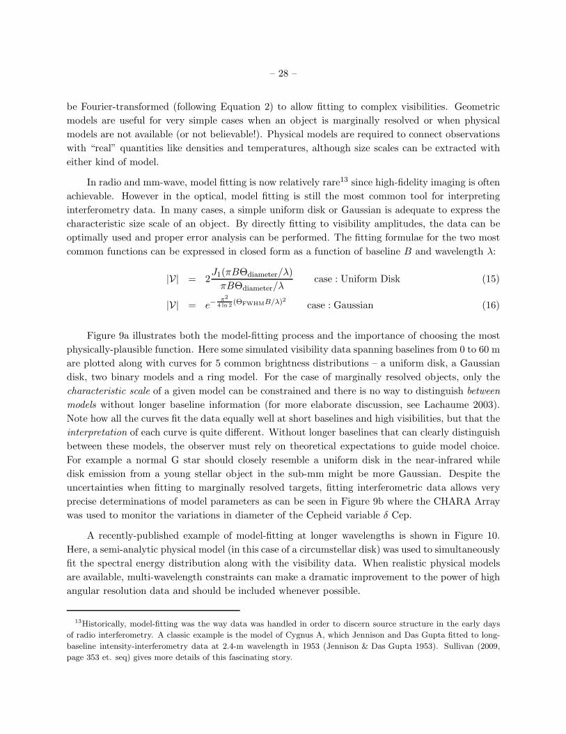
– 28 –

be Fourier-transformed (following Equation 2) to allow fitting to complex visibilities. Geometric

models are useful for very simple cases when an object is marginally resolved or when physical

models are not available (or not believable!). Physical models are required to connect observations

with “real” quantities like densities and temperatures, although size scales can be extracted with

either kind of model.

In radio and mm-wave, model fitting is now relatively rare13 since high-fidelity imaging is often

achievable. However in the optical, model fitting is still the most common tool for interpreting

interferometry data. In many cases, a simple uniform disk or Gaussian is adequate to express the

characteristic size scale of an object. By directly fitting to visibility amplitudes, the data can be

optimally used and proper error analysis can be performed. The fitting formulae for the two most

common functions can be expressed in closed form as a function of baseline B and wavelength λ:

|V| = 2J1(πBΘdiameter/λ)

πBΘdiameter/λcase : Uniform Disk (15)

|V| = e−π2

4 ln 2(ΘFWHMB/λ)2 case : Gaussian (16)

Figure 9a illustrates both the model-fitting process and the importance of choosing the most

physically-plausible function. Here some simulated visibility data spanning baselines from 0 to 60 m

are plotted along with curves for 5 common brightness distributions – a uniform disk, a Gaussian

disk, two binary models and a ring model. For the case of marginally resolved objects, only the

characteristic scale of a given model can be constrained and there is no way to distinguish between

models without longer baseline information (for more elaborate discussion, see Lachaume 2003).

Note how all the curves fit the data equally well at short baselines and high visibilities, but that the

interpretation of each curve is quite different. Without longer baselines that can clearly distinguish

between these models, the observer must rely on theoretical expectations to guide model choice.

For example a normal G star should closely resemble a uniform disk in the near-infrared while

disk emission from a young stellar object in the sub-mm might be more Gaussian. Despite the

uncertainties when fitting to marginally resolved targets, fitting interferometric data allows very

precise determinations of model parameters as can be seen in Figure 9b where the CHARA Array

was used to monitor the variations in diameter of the Cepheid variable δ Cep.

A recently-published example of model-fitting at longer wavelengths is shown in Figure 10.

Here, a semi-analytic physical model (in this case of a circumstellar disk) was used to simultaneously

fit the spectral energy distribution along with the visibility data. When realistic physical models

are available, multi-wavelength constraints can make a dramatic improvement to the power of high

angular resolution data and should be included whenever possible.

13Historically, model-fitting was the way data was handled in order to discern source structure in the early days

of radio interferometry. A classic example is the model of Cygnus A, which Jennison and Das Gupta fitted to long-

baseline intensity-interferometry data at 2.4-m wavelength in 1953 (Jennison & Das Gupta 1953). Sullivan (2009,

page 353 et. seq) gives more details of this fascinating story.

– 29 –

5. Synthesis imaging

Interferometer data in their raw form are not easy to visualize. Fortunately, as discussed in

§2.2, the measured complex visibilities can be transformed into an equivalent brightness distribution

on the sky – an image. This procedure is called “aperture synthesis imaging” or more generally

“synthesis imaging.” In this section, the critical data analysis steps are described for creating an

image in both the ideal case as well as more challenging scenarios when faced with poor (u,v)

coverage and phase instability.

5.1. Ideal case

Under ideal conditions the astronomer will have collected interferometer data with a large

number of telescopes including some Earth rotation to fill-in gaps in (u,v) coverage (see §3.2). In

addition, each datum will consist of a fully calibrated complex visibility – both amplitude and

phase information. Modern radio arrays such as the VLA and ALMA produce data of this quality

when proper phase-referencing procedures (see §3.1.3) are employed.

Figure 11 depicts the Fourier coverage for a 6 telescope interferometer along with the resulting

image from a direct Fourier transform of this coverage for a perfect point source (by construction,

the image will be purely real). In this procedure, the values in the (u,v) grid are set to unity where

data exists and to zero where no data exists. This resulting image shows artifacts because of the

missing (u,v) data that were zeroed out. These artifacts are often called “sidelobes” and show

both positive and negative excursions – note that negative flux density is usually a strong sign of a

sidelobe since negative values in an image are typically unphysical (except for special applications

like absorption line studies or polarization stokes mapping). Note that the central core of the

image represents the diffraction-limited angular resolution of this observation. Often in a practical

situation, the central core will be elongated because (u,v) coverage is not perfectly symmetric, with

longer baselines in some directions than others. The last panel in this figure shows the resulting

image for a binary star with 2:1 flux ratio. Notice that the image contains two sources, however

both sources show the same pattern of artifacts as the simple point source. Indeed, this supports

the previous assertion that missing (u,v) coverage is the main origin of this pattern and suggests

that the image quality can be improved by correcting for the sidelobe effect.

To proceed, the well-known Convolution Theorem must be introduced: Multiplication in the

“(u,v) space” is equivalent to a convolution in “image space.” Mathematically, this as can be

expressed:

FT(V(u, v) ·M(u, v)) = (FT V)⊗ (FT M) (17)

V(u, v) ·M(u, v) ⇔ I(x, y)⊗B(x, y) (18)

– 30 –

where V is the full underlying complex visibility that could in principle be measured by the inter-

ferometer, M is the (u,v) mask that encodes whether data exists (1) or is missing (0)14, FT and

⇔ denote a Fourier Transform, I = FT V is the true image distribution , and B = FT M is called

the “Convolving Beam.”

Application of the convolution theorem permits an elegant reformulation of the imaging prob-

lem into a “deconvolution” problem, where the convolving beam is a complicated function but

derived directly from M , the observed (u,v) coverage. Since M is exactly known, the convolving

beam B is known as well. Note that this deconvolution problem contrasts sharply with the decon-

volution problem in adaptive optics imaging where the point source function (PSF) varies in time

and is never precisely known.

5.1.1. CLEAN Algorithm

One of the earliest methods developed for deconvolution was the CLEAN algorithm (Hogbom

1974), which is still widely used in radio interferometry. In CLEAN, the Fourier transform of the

gridded complex visibility data is called the “dirty image” (or sometimes “dirty map”) and the

Fourier transform of the (u,v) plane mask is called the “dirty beam.” One first needs to deconvolve

the dirty image with the dirty beam. To do this, the true image I is interatively constructed by

locating the peak in the dirty image and subtracting from this a scaled version of the dirty beam

centered at this location. Here, the scaling of the dirty beam is typically tuned to removed a

certain fraction of intensity from the peak, often 5%. One keeps track of how much one removes

by collecting the “CLEAN” components in a list.

Consider this example. The dirty image has peak of 1.0 Jy at pixel location (3,10). One creates

a scaled dirty beam with a peak of 0.05 Jy, shifts the peak to the position (3,10), and subtracts

this scaled dirty beam from the dirty image. This CLEAN component is collected and labeled by

location (3,10) and flux contribution (0.05 Jy). Continue this procedure, flux is removed from dirty

image and CLEAN components are collected. This procedure is halted when the residual dirty

image contains only noise. Since the intensity in the true image is expected to be positive-definite,

one common criterion for halting the CLEAN cycles is when the largest negative value in the image

is comparable to the largest positive value in the image, thereby avoiding any CLEAN components

having negative flux.

In principle, this collection of delta function point sources (all the CLEAN components) is

the best estimate of the image distribution. However, an image of point sources is not visually

appealing and a common procedure is to convolve the point source distribution with a “CLEAN”

beam, a perfect 2-D Gaussian with a core that matches the FWHM of the dirty beam. Commonly,

14In general, one can consider a full “Spatial Transfer Function” which can have weights between 0 and 1. Here,

consider just a simple binary mask in the (u,v) plane for simplicity.

– 31 –

a filled ellipse will be included in the corner of a CLEANed image showing the 2D FWHM of the

restoring beam. Lastly, one adds back the residual image from the dirty map (which should contain

only noise) so that the noise level is apparent in the final image and remnant uncorrected sidelobe

artifacts, if present, can be readily identified. These steps are illustrated in Figure 12 where the

CLEAN procedure has been applied to the examples shown in Figure 11.

The steps of the CLEAN algorithm are summarized below.

1. Create dirty map and beam.

2. Find peak of dirty map.

3. Subtract scaled version of dirty beam from dirty map, removing a small percentage (e.g.,

∼5%) of peak intensity. Collect CLEAN components.

4. Repeat last step until negative residuals are comparable to positive residuals.

5. Convolve CLEAN components with CLEAN beam.

6. Add back the residuals.

While it is beyond the scope to address the weaknesses of the CLEAN algorithm in detail,

a few issues are worth mentioning in passing. Typical CLEAN algorithms do not naturally deal

with errors unless all the visibility data are of similar quality. The case when each visibility point

is weighted equally is called natural weighting (which gives best SNR for detecting faint objects)

and the case when each portion of the (u,v) plane is equally weighted, so called uniform weighting

(which gives somewhat higher angular resolution but at some loss of sensitivity). Briggs (1995)

introduced a “ROBUST” parameter than can naturally span these two extremes. Other problems

with CLEAN include difficulty reconstructing low surface brightness regions, large scale emission

and the fact that the final reconstructed image is of a degraded resolution because the convolving

PSF actually suppresses the longest baseline visibilities from the final image. Finally, if the imaging

step makes use of the Fast Fourier Transform, several additional artifacts can appear in the image

as a consequence of the necessity to grid the input u, v data.

5.1.2. Maximum Entropy Method (MEM)

Another common method for reconstructing images from interferometric data is called the

Maximum Entropy Method (Gull & Skilling 1983; Skilling & Bryan 1984). This approach asks the

question: “How to choose which reconstructed image is best, considering that there are an infinite

number of images that can fit the interferometer dataset within the statistical uncertainties?” The

simple answer here is that the “best” image is the one that both fits the data acceptably and also

maximizes the Entropy S defined as:

– 32 –

S = −∑

i

fi lnfimi

(19)

where fi is the (positive-definite) fraction of flux in pixel i, and mi is called the image prior which

can encapsulate prior knowledge of the flux distribution (e.g., known from physical considerations

or lower resolution observations). Narayan & Nityananda (1986) describe general properties of this

algorithm in a lucid review article and motivates the above methodology using Bayes’ Theorem,

the cornerstone of so-called Bayesian Statistics.

Entropy is an interesting statistic since it quantifies the amount of complexity in a distribution.

It is often stated that MEM tries to find the “smoothest image” consistent with the data. This

indeed is a highly desirable feature since any structures in the reconstructed image should be based

on the data itself and not artifacts from the reconstruction process. However, MEM does not

actually select the smoothest image but rather one with “most equal” uniform set of values – MEM

does not explicitly take into account spatial structure but only depends on the distribution of pixel

values. Indeed with more study, the Maximum Entropy functional has been found not to be that

special, except for its privileged appearance in physics. From a broader perspective, maximum

entropy can be considered one member of a class of regularizers that allow the inverse problem to

be well-defined, and MEM is not necessarily the best nor even suitable for some imaging problems

(e.g., other regularizers include total variation or maximum likelihood).

MEM performs better for reconstructing smooth large scale emission than CLEAN, although

MEM is much more computationally demanding. MEM can naturally deal with heterogeneous data

with varying errors since the data is essentially fitted using a χ2-like statistic. This involves only a

“forward” transform from image space to (u,v) space, thus avoiding all the issues of zeros in the (u,v)

grid and the need for deconvolution. In addition, MEM images possess super-resolution beyond

the traditional ∼ λD diffraction limit since smoothness is introduced in the process only indirectly

through the Entropy statistic. For instance, if the object is a point-like object, then the FWHM

of the reconstructed MEM image depends on the signal-to-noise of the data, not just the length

of the longest baseline. Super-resolution is viewed with some skepticism by practioners of CLEAN

because structures beyond the formal diffraction limit may be artifacts of the Entropy functional.

MEM has been implemented in many radio interferometry data processing environments, such as

AIPS for VLA/VLBA, Caltech VLBI package (Sivia 1987), and for optical interferometry (e.g.,

BSMEM, Buscher 1994).

5.2. Non-ideal cases for imaging

Most modern interferometric arrays in the radio (VLA) and millimeter (ALMA, CARMA) have

a sufficient number of elements for good (u,v) coverage and also employ rapid phase referencing

for absolute phase calibration. This allows either CLEAN and MEM methods to make imaging

possible, although mosaicing large fields can still pose a computational challenge.

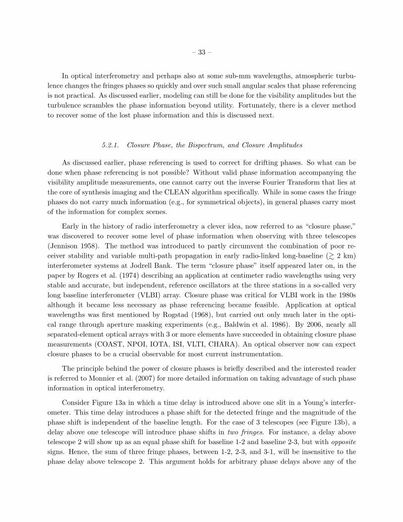
– 33 –

In optical interferometry and perhaps also at some sub-mm wavelengths, atmospheric turbu-

lence changes the fringes phases so quickly and over such small angular scales that phase referencing

is not practical. As discussed earlier, modeling can still be done for the visibility amplitudes but the

turbulence scrambles the phase information beyond utility. Fortunately, there is a clever method

to recover some of the lost phase information and this is discussed next.

5.2.1. Closure Phase, the Bispectrum, and Closure Amplitudes

As discussed earlier, phase referencing is used to correct for drifting phases. So what can be

done when phase referencing is not possible? Without valid phase information accompanying the

visibility amplitude measurements, one cannot carry out the inverse Fourier Transform that lies at

the core of synthesis imaging and the CLEAN algorithm specifically. While in some cases the fringe

phases do not carry much information (e.g., for symmetrical objects), in general phases carry most

of the information for complex scenes.

Early in the history of radio interferometry a clever idea, now referred to as “closure phase,”

was discovered to recover some level of phase information when observing with three telescopes

(Jennison 1958). The method was introduced to partly circumvent the combination of poor re-

ceiver stability and variable multi-path propagation in early radio-linked long-baseline (& 2 km)

interferometer systems at Jodrell Bank. The term “closure phase” itself appeared later on, in the

paper by Rogers et al. (1974) describing an application at centimeter radio wavelengths using very

stable and accurate, but independent, reference oscillators at the three stations in a so-called very

long baseline interferometer (VLBI) array. Closure phase was critical for VLBI work in the 1980s

although it became less necessary as phase referencing became feasible. Application at optical

wavelengths was first mentioned by Rogstad (1968), but carried out only much later in the opti-

cal range through aperture masking experiments (e.g., Baldwin et al. 1986). By 2006, nearly all

separated-element optical arrays with 3 or more elements have succeeded in obtaining closure phase

measurements (COAST, NPOI, IOTA, ISI, VLTI, CHARA). An optical observer now can expect

closure phases to be a crucial observable for most current instrumentation.

The principle behind the power of closure phases is briefly described and the interested reader

is referred to Monnier et al. (2007) for more detailed information on taking advantage of such phase

information in optical interferometry.

Consider Figure 13a in which a time delay is introduced above one slit in a Young’s interfer-

ometer. This time delay introduces a phase shift for the detected fringe and the magnitude of the

phase shift is independent of the baseline length. For the case of 3 telescopes (see Figure 13b), a

delay above one telescope will introduce phase shifts in two fringes. For instance, a delay above

telescope 2 will show up as an equal phase shift for baseline 1-2 and baseline 2-3, but with opposite

signs. Hence, the sum of three fringe phases, between 1-2, 2-3, and 3-1, will be insensitive to the

phase delay above telescope 2. This argument holds for arbitrary phase delays above any of the

– 34 –

three telescopes. In general, the sum of three phases around a closed triangle of baselines, the

closure phase, is a good interferometric observable; that is, it is independent of telescope-specific

phase shifts induced by the atmosphere or optics.

The closure phase Φijk can thus be written in terms of the three telescopes i,j,k in the triangle:

Φijk = φij + φjk + φki (20)

where φij represents the measured Fourier phase for the baseline connecting telescopes i,j. Alter-

natively, the closure phase can be written in terms of the (u0,v0,u1,v1) in the Fourier (hyper-)plane

where (u0,v0) represents the (u,v) coverage for baseline i, j in the triangle, (u1,v1) represents the

(u,v) coverage for baseline j, k in the triangle, and the last leg of the triangle can be calculated

from the others since the sum of the 3 baselines must equal zero to be a “closure triangle.” See

definition and explanation put forward in documentation of the OI-FITS data format (Pauls et al.

2005).

Another method to derive the invariance of the closure phase to telescope-specific phase shifts

is through the bispectrum. The bispectrum Bijk = Vij VjkVki is formed through triple products of

the complex visibilities around a closed triangle, where ijk specifies the three telescopes. Using Eq.

14 and using the concept of telescope-specific complex gains Gi, it can be seen how the telescope-

specific errors affect the measured bispectrum:

Bijk = Vmeasured

ij Vmeasured

jk Vmeasured

ki (21)

= |Gi||Gj |ei(ΦGi −ΦG

j )V true

ij · |Gj ||Gk|ei(ΦGj −ΦG

k)V true

jk · |Gk||Gi|ei(ΦGk−ΦG

i )V true

ki (22)

= |Gi|2|Gj |2|Gk|2V true

ij · V true

jk · V true

ki (23)

From the above derivation, the bispectrum is a complex quantity whose phase is identical to the

closure phase, while the individual telescope gains affect only the bispectrum amplitude. The use

of the bispectrum for reconstructing diffraction-limited images from speckle data was developed

independently (Weigelt 1977) of the closure phase techniques, and the connection between the

approaches elucidated only later (Roddier 1986; Cornwell 1987).

A 3-telescope array with its one triangle can provide a single closure phase measurement,

a paltry substitute for the 3 Fourier phases available using phase referencing. However, as one

increases the number of elements in the array from 3 telescopes to 7 telescopes, the number of

independent closure phases increases dramatically to 15, about 70% of the total 21 Fourier phases

available. An array the size of the VLA with 27 antennae is capturing 93% of the phase information.

Indeed, imaging of bright objects does not require phase referencing and the VLA can make high

quality imaging through closure phases alone. Note that imaging using closure phases alone retains

no absolute astrometry information; astrometry requires phase-referencing.

A related quantity useful in radio is the closure amplitude (which requires sets of 4 telescopes)

and this can be used to compensate for unstable amplifier gains and varying antenna efficiencies

– 35 –

(e.g., Readhead et al. 1980). Closure amplitudes are not practical for current optical interferometers

partially because most fringe amplitude variations are not caused by telescope-specific gain changes

but rather by changing coherence (e.g., due to changing atmosphere).

Closure phases (and closure amplitudes) can be introduced into the imaging process in a variety

of ways. For the CLEAN algorithm, the closure phases can not be directly used because CLEAN

requires estimates of the actual Fourier phases in order to carry out a Fourier transform. A clever

iterative scheme known as self-calibration was described by Readhead & Wilkinson (1978) and

Cornwell & Wilkinson (1981) which alternates between a CLEANing stage and a self-calibration

stage that estimates Fourier phases from the closure phases and most recent CLEANed image. As

for standard CLEAN itself, self-calibration can not naturally deal with errors in the closure phases

and closure amplitudes, and thus is recognized as not optimal. That said, self-calibration is still

widely used along with CLEAN even in the case of phase referencing to dramatically improve the

imaging dynamic range for imaging of and around bright objects.

Closure phases, the bispectrum, and closure amplitudes can be quite naturally incorporated

into “forward-transform” image reconstruction schemes such as the Maximum Entropy Method.

Recall that MEM basically performs a minimization of a regularizer constrained by some goodness-

of-fit to the observed data. Thus, the bispectral quantities can be fitted just like all other ob-

servables. That said, the mathematics can be difficult and the program BSMEM (Buscher 1994)

was one of the first useful software suitable for optical interferometers that successfully solved

this problem in practice. Currently, the optical interferometer community have produced sev-

eral algorithms to solve this problem, including the Building Block Method (Hofmann & Weigelt

1993), MACIM (Ireland et al. 2006), MIRA (Thiebaut 2008), WISARD (Meimon et al. 2008), and

SQUEEZE (Baron et al. 2010). See Malbet et al. (2010) for a description of a recent blind imaging

competition between some of these algorithms.

5.3. Astrometry

Astrometry is still a specialized technique within interferometry and a detailed description is

beyond the scope of this chapter. Typically, the precise separation between two objects on the sky,

the relative astrometry, is needed to be known for some purpose, such as a parallax measurement. If

both objects are known point-like objects with no asymmetric structure, then the precise knowledge

of the baseline geometry can be used, along with detailed measurements of interferometric fringe

phase, to estimate their angular separation. In general, the astrometric precision ∆Φ on the sky is

related to the measured fringe phase SNR as follows:

∆Φ ∼ λ

Baseline· 1

SNR(24)

Hence, if one measures a fringe with a signal-to-noise of 100 (which is quite feasible) then one

can determine the relative separation of two sources with a precision 100× smaller than the fringe

– 36 –

spacing. Since VLBI and optical interferometers have fringe spacings of ∼1 milliarcseconds, this

allows for astrometric precision at the 10 microarcsecond level allowing parallax measurements at

many kiloparsecs and also allows us to take a close look around the black hole at the center of the

Galaxy. Unfortunately, at this precision level many systematic effects become critical and knowl-

edge of the absolute baseline vector between telescopes is crucial and demanding. The interested

reader should consult specific instruments and recent results for more information (Reid et al. 2009;

Muterspaugh et al. 2010, for radio and optical respectively).

6. Concluding remarks

In barely more than 50 years, separated-element interferometry has come to dominate radio

telescope design as the science has demanded ever-increasing angular resolution. The addition of

more elements to an array has provided improvements both in mapping speed and in sensitivity.

The early problems with instability in the electronics were solved years ago by improvements in

radio and digital electronics, and it is presently not unusual to routinely achieve interferometer

phase stability of order λ/1000 over time spans of many tens of minutes. Sensitivity improve-

ments by further reductions in receiver temperature are reaching a point of diminishing returns as

the remaining contributions from local spillover, the Galactic background, and atmospheric losses

come to dominate the equation. Advances in the speed and density of digital solid-state devices

are presently driving the development of increased sensitivity, with flexible digital signal proces-

sors providing wider bands for continuum observations and high frequency resolution for precision

spectroscopy. With the commissioning of the billion-dollar international facility ALMA underway

and long-term plans for ambitious arrays at longer wavelengths (SKA, LOFAR), the future of “ra-

dio” interferometry is bright and astronomers are eager to take advantage of the new capabilities,

especially vast improvements to sensitivity.

The younger field of optical interferometry is still rapidly developing with innovative beam

combination, fringe tracking methods and extensions of adaptive optics promising significant im-

provements in sensitivity for years to come. In the long-run however, the atmosphere poses a

fundamental limit to the ultimate astrometric precision and absolute sensitivity for visible and

infrared interferometry that can only be properly overcome by placing the telescopes into space or

through exploring exotic sites such as Dome A, Antarctica. Currently however, the emphasis of

the majority of the scientific community favors ever-larger collecting area in the near- and mid-IR

(e.g. JWST) as astronomers reach to ever greater distances and earlier times, rather than higher

angular resolution.

Eventually, the limits of diffraction are likely to limit the science return of space telescopes,

and the traditional response of building a larger aperture will no longer be affordable. Filled aper-

tures increase in weight and in cost as a power > 1 of the diameter (Bely 2003). For ground-based

telescopes, cost ∼ D2.6. In space, the growth is slower, ∼ D1.6, although the coefficient of pro-

– 37 –

portionality is much larger15. Over the last two decades the prospects have become increasingly

bleak for building ever larger filled-aperture telescopes within the anticipated space science bud-

gets. Interferometry permits the connection of individual collectors of modest size and cost into

truly gigantic space-based constellations with virtually unlimited angular resolution (Allen 2007).

Ultimately, the pressure of discovery is likely to make interferometry in space at optical, UV, and

IR wavelengths a necessity, just as it did at radio wavelengths more than half a century earlier.

A. Appendix: Current Facilities

Table 4 provides a comprehensive list of existing and planned interferometer facilities. These

facilities span the range from “private” instruments, currently available only to their developers,

to general purpose instruments. An example of the latter is the Square Kilometer Array; this is a

major next-generation facility for radio astronomy being planned by an international consortium,

with a Project Office at the Jodrell Bank Observatory in the UK (http://www.skatelescope.org/).

The location for the SKA has not yet been finalized, but (as of 2011) sites in Australia and South

Africa are currently being discussed. Plans for the SKA have spawned several ”proof-of-concept” or

”pathfinder” instruments which are being designed and built including LOFAR (Europe), MeerKAT

(South Africa), ASKAP, MWA, and SKAMP (Australia), and LWA (USA).

Table 5 summarizes the wavelength and angular resolution of currently operating arrays open

to the general astronomer. A few of the facilities in this list are still under construction. Figure 14

summarizes the vast wavelength range and angular resolution available using the radio and optical

interferometers of the world.

15It’s interesting to note that at some large-enough diameter, ground-based telescopes are likely to become similar

in cost to those in space, especially if one considers life-cycle costs.

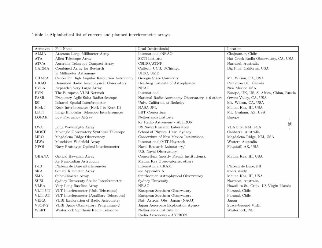
–38

–Table 4: Alphabetical list of current and planned interferometer arrays.

Acronym Full Name Lead Institution(s) Location

ALMA Atacama Large Millimeter Array International/NRAO Chajnantor, Chile

ATA Allen Telescope Array SETI Institute Hat Creek Radio Observatory, CA, USA

ATCA Australia Telescope Compact Array CSIRO/ATNF Narrabri, Australia

CARMA Combined Array for Research Caltech, UCB, UChicago, Big Pine, California USA

in Millimeter Astronomy UIUC, UMD

CHARA Center for High Angular Resolution Astronomy Georgia State University Mt. Wilson, CA, USA

DRAO Dominion Radio Astrophysical Observatory Herzberg Institute of Astrophysics Penticton BC, Canada

EVLA Expanded Very Large Array NRAO New Mexico USA

EVN The European VLBI Network International Europe, UK, US, S. Africa, China, Russia

FASR Frequency Agile Solar Radiotelescope National Radio Astronomy Observatory + 6 others Owens Valley, CA, USA

ISI Infrared Spatial Interferometer Univ. California at Berkeley Mt. Wilson, CA, USA

Keck-I Keck Interferometer (Keck-I to Keck-II) NASA-JPL Mauna Kea, HI, USA

LBTI Large Binocular Telescope Interferometer LBT Consortium Mt. Graham, AZ, USA

LOFAR Low Frequency ARray Netherlands Institute Europe

for Radio Astronomy - ASTRON

LWA Long Wavelength Array US Naval Research Laboratory VLA Site, NM, USA

MOST Molonglo Observatory Synthesis Telescope School of Physics, Univ. Sydney Canberra, Australia

MRO Magdalena Ridge Observatory Consortium of New Mexico Institutions, Magdalena Ridge, NM, USA

MWA Murchison Widefield Array International/MIT-Haystack Western Australia

NPOI Navy Prototype Optical Interferometer Naval Research Laboratory/ Flagstaff, AZ, USA

U.S. Naval Observatory

OHANA Optical Hawaiian Array Consortium (mostly French Institutions), Mauna Kea, HI, USA

for Nanoradian Astronomy Mauna Kea Observatories, others

PdB Plateau de Bure interferometer International/IRAM Plateau de Bure, FR

SKA Square Kilometer Array see Appendix A under study

SMA Submillimeter Array Smithsonian Astrophysical Observatory Mauna Kea, HI, USA

SUSI Sydney University Stellar Interferometer Sydney University Narrabri, Australia

VLBA Very Long Baseline Array NRAO Hawaii to St. Croix, US Virgin Islands

VLTI-UT VLT Interferometer (Unit Telescopes) European Southern Observatory Paranal, Chile

VLTI-AT VLT Interferometer (Auxiliary Telescopes) European Southern Observatory Paranal, Chile

VERA VLBI Exploration of Radio Astrometry Nat. Astron. Obs. Japan (NAOJ) Japan

VSOP-2 VLBI Space Observatory Programme-2 Japan Aerospace Exploration Agency Space-Ground VLBI

WSRT Westerbork Synthesis Radio Telescope Netherlands Institute for Westerbork, NL

Radio Astronomy - ASTRON

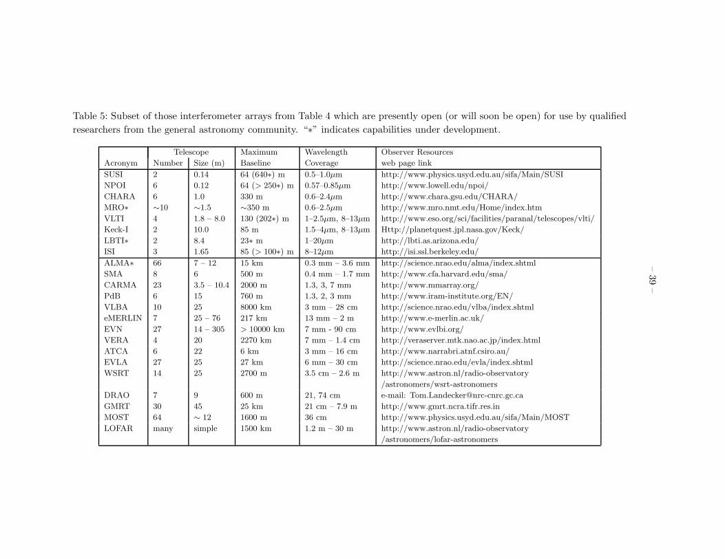
–39

–

Table 5: Subset of those interferometer arrays from Table 4 which are presently open (or will soon be open) for use by qualified

researchers from the general astronomy community. “∗” indicates capabilities under development.

Telescope Maximum Wavelength Observer Resources

Acronym Number Size (m) Baseline Coverage web page link

SUSI 2 0.14 64 (640∗) m 0.5–1.0µm http://www.physics.usyd.edu.au/sifa/Main/SUSI

NPOI 6 0.12 64 (> 250∗) m 0.57–0.85µm http://www.lowell.edu/npoi/

CHARA 6 1.0 330 m 0.6–2.4µm http://www.chara.gsu.edu/CHARA/

MRO∗ ∼10 ∼1.5 ∼350 m 0.6–2.5µm http://www.mro.nmt.edu/Home/index.htm

VLTI 4 1.8 – 8.0 130 (202∗) m 1–2.5µm, 8–13µm http://www.eso.org/sci/facilities/paranal/telescopes/vlti/

Keck-I 2 10.0 85 m 1.5–4µm, 8–13µm Http://planetquest.jpl.nasa.gov/Keck/

LBTI∗ 2 8.4 23∗ m 1–20µm http://lbti.as.arizona.edu/

ISI 3 1.65 85 (> 100∗) m 8–12µm http://isi.ssl.berkeley.edu/

ALMA∗ 66 7 – 12 15 km 0.3 mm – 3.6 mm http://science.nrao.edu/alma/index.shtml

SMA 8 6 500 m 0.4 mm – 1.7 mm http://www.cfa.harvard.edu/sma/

CARMA 23 3.5 – 10.4 2000 m 1.3, 3, 7 mm http://www.mmarray.org/

PdB 6 15 760 m 1.3, 2, 3 mm http://www.iram-institute.org/EN/

VLBA 10 25 8000 km 3 mm – 28 cm http://science.nrao.edu/vlba/index.shtml

eMERLIN 7 25 – 76 217 km 13 mm – 2 m http://www.e-merlin.ac.uk/

EVN 27 14 – 305 > 10000 km 7 mm - 90 cm http://www.evlbi.org/

VERA 4 20 2270 km 7 mm – 1.4 cm http://veraserver.mtk.nao.ac.jp/index.html

ATCA 6 22 6 km 3 mm – 16 cm http://www.narrabri.atnf.csiro.au/

EVLA 27 25 27 km 6 mm – 30 cm http://science.nrao.edu/evla/index.shtml

WSRT 14 25 2700 m 3.5 cm – 2.6 m http://www.astron.nl/radio-observatory

/astronomers/wsrt-astronomers

DRAO 7 9 600 m 21, 74 cm e-mail: Tom.Landecker@nrc-cnrc.gc.ca

GMRT 30 45 25 km 21 cm – 7.9 m http://www.gmrt.ncra.tifr.res.in

MOST 64 ∼ 12 1600 m 36 cm http://www.physics.usyd.edu.au/sifa/Main/MOST

LOFAR many simple 1500 km 1.2 m – 30 m http://www.astron.nl/radio-observatory

/astronomers/lofar-astronomers

– 40 –

We are grateful to the following colleagues for their comments and contributions: W.M. Goss,

R.D. Ekers, T.L. Wilson, S. Kraus, M. Zhao, T. ten Brummelaar, A. King, and P. Teuben.

REFERENCES

Allen, R. J. 2007, PASP, 119, 914

Allen, R. J., Goss, W. M., & van Woerden, H. 1973, A&A, 29, 447

Andrews, S. M., Wilner, D. J., Hughes, A. M., Qi, C., & Dullemond, C. P. 2009, ApJ, 700, 1502

Baade, W. & Minkowski, R. 1954, ApJ, 119, 206

Baldwin, J. E., Beckett, M. G., Boysen, R. C., Burns, D., Buscher, D. F., Cox, G. C., Haniff, C. A.,

Mackay, C. D., Nightingale, N. S., Rogers, J., Scheuer, P. A. G., Scott, T. R., Tuthill, P. G.,

Warner, P. J., Wilson, D. M. A., & Wilson, R. W. 1996, A&A, 306, L13

Baldwin, J. E., Haniff, C. A., Mackay, C. D., & Warner, P. J. 1986, Nature, 320, 595

Baron, F., Monnier, J. D., & Kloppenborg, B. 2010, in Society of Photo-Optical Instrumentation

Engineers (SPIE) Conference, Vol. 7734, Society of Photo-Optical Instrumentation Engineers

(SPIE) Conference Series

Bely, P. Y. 2003, The Design and Construction of Large Optical Telescopes (Springer)

Bolton, J. G., Stanley, G. J., & Slee, O. B. 1949, Nature, 164, 101

Bosma, A. 1981a, AJ, 86, 1791

—. 1981b, AJ, 86, 1825

Bridle, A. H., Hough, D. H., Lonsdale, C. J., Burns, J. O., & Laing, R. A. 1994, AJ, 108, 766

Briggs, D. S. 1995, in Bulletin of the American Astronomical Society, Vol. 27, American Astronom-

ical Society Meeting Abstracts, # 112.02

Buscher, D. F. 1994, in IAU Symposium, Vol. 158, Very High Angular Resolution Imaging, ed.

J. G. Robertson & W. J. Tango, 91

Carilli, C. L. & Holdaway, M. A. 1999, Radio Science, 34, 817

Cohen, M. H., Cannon, W., Purcell, G. H., Shaffer, D. B., Broderick, J. J., Kellermann, K. I., &

Jauncey, D. L. 1971, ApJ, 170, 207

Colavita, M. M. 1999, PASP, 111, 111

– 41 –

Colavita, M. M., Serabyn, E., Millan-Gabet, R., Koresko, C. D., Akeson, R. L., Booth, A. J.,

Mennesson, B. P., Ragland, S. D., Appleby, E. C., Berkey, B. C., Cooper, A., Crawford,

S. L., Creech-Eakman, M. J., Dahl, W., Felizardo, C., Garcia-Gathright, J. I., Gathright,

J. T., Herstein, J. S., Hovland, E. E., Hrynevych, M. A., Ligon, E. R., Medeiros, D. W.,

Moore, J. D., Morrison, D., Paine, C. G., Palmer, D. L., Panteleeva, T., Smith, B., Swain,

M. R., Smythe, R. F., Summers, K. R., Tsubota, K., Tyau, C., Vasisht, G., Wetherell, E.,

Wizinowich, P. L., & Woillez, J. M. 2009, PASP, 121, 1120

Cornwell, T. J. 1987, A&A, 180, 269

Cornwell, T. J. & Wilkinson, P. N. 1981, MNRAS, 196, 1067

Danchi, W. C., Bester, M., Degiacomi, C. G., Greenhill, L. J., & Townes, C. H. 1994, AJ, 107,

1469

Delplancke, F., Derie, F., Lev”que, S., Menardi, S., Abuter, R., Andolfato, L., Ballester, P., de

Jong, J., Di Lieto, N., Duhoux, P., Frahm, R., Gitton, P., Glindemann, A., Palsa, R.,

Puech, F., Sahlmann, J., Schuhler, N., Duc, T. P., Valat, B., & Wallander, A. 2006, in

Society of Photo-Optical Instrumentation Engineers (SPIE) Conference, Vol. 6268, Society

of Photo-Optical Instrumentation Engineers (SPIE) Conference Series

di Benedetto, G. P. & Rabbia, Y. 1987, A&A, 188, 114

Fried, D. L. 1965, J. Opt. Soc. Am., 55, 1427

Glindemann, A. 2010, Principles of Stellar Interferometry (Springer-Verlag)

Golay, M. 1971, J. Opt. Soc. Am., 61, 272

Goss, W. M., Brown, R. L., & Lo, K. Y. 2003, Astronomische Nachrichten Supplement, 324, 497

Greenhill, L. J., Gwinn, C. R., Schwartz, C., Moran, J. M., & Diamond, P. J. 1998, Nature, 396,

650

Gull, S. F. & Skilling, J. 1983, in Indirect Imaging. Measurement and Processing for Indirect

Imaging. Proceedings of an International Symposium held in Sydney, Australia, August

30-September 2, 1983. Editor, J.A. Roberts; Publisher, Cambridge University Press, 267

Hanbury Brown, R., Davis, J., & Allen, L. R. 1974, MNRAS, 167, 121

Hecht, E. 2002, Optics (Boston: Addison-Wesley)

Heffner, H. 1962, Proc. IRE, 50, 1604

Hofmann, K. & Weigelt, G. 1993, A&A, 278, 328

Hogbom, J. A. 1974, A&AS, 15, 417

– 42 –

Holdaway, M. A. & Helfer, T. T. 1999, in Astronomical Society of the Pacific Conference Series, Vol.

180, Synthesis Imaging in Radio Astronomy II, ed. G. B. Taylor, C. L. Carilli, & R. A. Perley,

537

Ireland, M. J., Monnier, J. D., & Thureau, N. 2006, in Society of Photo-Optical Instrumentation

Engineers (SPIE) Conference, Vol. 6268, Advances in Stellar Interferometry. Edited by Mon-

nier, John D.; Scholler, Markus; Danchi, William C.. Proceedings of the SPIE, Volume 6268,

pp. 62681T (2006).

Jennison, R. C. 1958, MNRAS, 118, 276

Jennison, R. C. & Das Gupta, M. K. 1953, Nature, 172, 996

Johnson, M. A., Betz, A. L., & Townes, C. H. 1974, Physical Review Letters, 33, 1617

Keto, E. 1997, ApJ, 475, 843

Kishimoto, M., Honig, S. F., Antonucci, R., Kotani, T., Barvainis, R., Tristram, K. R. W., &

Weigelt, G. 2009, A&A, 507, L57

Kraus, S., Hofmann, K., Benisty, M., Berger, J., Chesneau, O., Isella, A., Malbet, F., Meilland, A.,

Nardetto, N., Natta, A., Preibisch, T., Schertl, D., Smith, M., Stee, P., Tatulli, E., Testi,

L., & Weigelt, G. 2008, A&A, 489, 1157

Labeyrie, A. 1975, ApJ, 196, L71

Labeyrie, A., Lipson, S. G., & Nisenson, P. 2006, An Introduction to Optical Stellar Interferometry

(Cambridge University Press)

Lachaume, R. 2003, A&A, 400, 795

Lane, B. F., Kuchner, M. J., Boden, A. F., Creech-Eakman, M., & Kulkarni, S. R. 2000, Nature,

407, 485

Lawson, P. R., ed. 2000, Principles of Long Baseline Stellar Interferometry

Malbet, F., Cotton, W., Duvert, G., Lawson, P., Chiavassa, A., Young, J., Baron, F., Buscher, D.,

Rengaswamy, S., Kloppenborg, B., Vannier, M., & Mugnier, L. 2010, in Society of Photo-

Optical Instrumentation Engineers (SPIE) Conference, Vol. 7734, Society of Photo-Optical

Instrumentation Engineers (SPIE) Conference Series

Malbet, F. & Perrin, G., eds. 2007, Proceedings of the Euro Summer School ”Observation and Data

Reduction with with the VLT Interferometer” (New Astronomy Reviews), Vol. 51, 563–564

McCready, L. L., Pawsey, J. L., & Payne-Scott, R. 1947, Royal Society of London Proceedings

Series A, 190, 357

– 43 –

Meimon, S., Mugnier, L. M., & Le Besnerais, G. 2008, Journal of the Optical Society of America

A, 26, 108

Merand, A., Kervella, P., Coude du Foresto, V., Ridgway, S. T., Aufdenberg, J. P., ten Brummelaar,

T. A., Berger, D. H., Sturmann, J., Sturmann, L., Turner, N. H., & McAlister, H. A. 2005,

A&A, 438, L9

Michelson, A. A. & Pease, F. G. 1921, ApJ, 53, 249

Millan-Gabet, R., Schloerb, F. P., & Traub, W. A. 2001, ApJ, 546, 358

Miyoshi, M., Moran, J., Herrnstein, J., Greenhill, L., Nakai, N., Diamond, P., & Inoue, M. 1995,

Nature, 373, 127

Monnier, J. D. 2003, Reports on Progress in Physics, 66, 789

Monnier, J. D., Berger, J.-P., Millan-Gabet, R., Traub, W. A., Schloerb, F. P., Pedretti, E.,

Benisty, M., Carleton, N. P., Haguenauer, P., Kern, P., Labeye, P., Lacasse, M. G., Malbet,

F., Perraut, K., Pearlman, M., & Zhao, M. 2006, ApJ, 647, 444

Monnier, J. D., Zhao, M., Pedretti, E., Thureau, N., , M., Muirhead, P., Berger, J., Millan-Gabet,

R., Van Belle, G., ten Brummelaar, T., McAlister, H., Ridgway, S., Turner, N., Sturmann,

L., Sturmann, J., & Berger, D. 2007, Science, 317, 342

Muterspaugh, M. W., Lane, B. F., Kulkarni, S. R., Konacki, M., Burke, B. F., Colavita, M. M.,

Shao, M., Wiktorowicz, S. J., & O’Connell, J. 2010, AJ, 140, 1579

Narayan, R. & Nityananda, R. 1986, ARA&A, 24, 127

Oliver, B. M. 1965, Proc. IEEE, 53, 436

Pathria, R. K. 1972, Statistical Mechanics (Pergamon Press)

Pauls, T. A., Young, J. S., Cotton, W. D., & Monnier, J. D. 2005, PASP, 117, 1255

Pawsey, J. L., Payne-Scott, R., & McCready, L. L. 1946, Nature, 157, 158

Peterson, D. M., Hummel, C. A., Pauls, T. A., Armstrong, J. T., Benson, J. A., Gilbreath, G. C.,

Hindsley, R. B., Hutter, D. J., Johnston, K. J., Mozurkewich, D., & Schmitt, H. R. 2006,

Nature, 440, 896

Porcas, R. W., Booth, R. S., Browne, I. W. A., Walsh, D., & Wilkinson, P. N. 1979, Nature, 282,

385

Quirrenbach, A. 2000, in Principles of Long Baseline Stellar Interferometry, 71

Quirrenbach, A. 2001, ARA&A, 39, 353

– 44 –

Quirrenbach, A., Bjorkman, K. S., Bjorkman, J. E., Hummel, C. A., Buscher, D. F., Armstrong,

J. T., Mozurkewich, D., Elias, II, N. M., & Babler, B. L. 1997, ApJ, 479, 477

Readhead, A., Nakajima, T., Pearson, T., Neugebauer, G., Oke, J., & Sargent, W. 1988, AJ, 95,

1278

Readhead, A. C. S., Walker, R. C., Pearson, T. J., & Cohen, M. H. 1980, Nature, 285, 137

Readhead, A. C. S. & Wilkinson, P. N. 1978, ApJ, 223, 25

Reid, M. J., Menten, K. M., Brunthaler, A., Zheng, X. W., Moscadelli, L., & Xu, Y. 2009, ApJ,

693, 397

Roddier, F. 1986, Optics Communications, 60, 145

Rogers, A. E. E., Hinteregger, H. F., Whitney, A. R., Counselman, C. C., Shapiro, I. I., Wittels,

J. J., Klemperer, W. K., Warnock, W. W., Clark, T. A., & Hutton, L. K. 1974, ApJ, 193,

293

Rogstad, D. H. 1968, Applied Optics, 7, 585+

Rogstad, D. H. & Shostak, G. S. 1972, ApJ, 176, 315

Rots, A. H. 1975, A&A, 45, 43

Rots, A. H. & Shane, W. W. 1975, A&A, 45, 25

Saha, S. K. 2011, Aperture Synthesis (Springer)

Shao, M. & Colavita, M. M. 1992, A&A, 262, 353

Sivia, D. 1987, PhD thesis, Cambridge University

Skilling, J. & Bryan, R. K. 1984, MNRAS, 211, 111

Smith, F. G. 1951, Nature, 168, 555

Sullivan, W. T. 2009, Cosmic Noise (Cambridge: Cambridge University Press)

Sutton, E. C. & Hueckstaedt, R. M. 1996, A&AS, 119, 559

Taylor, G. B., Carilli, C. L., & Perley, R. A., eds. 1999, Astronomical Society of the Pacific

Conference Series, Vol. 180, Synthesis Imaging in Radio Astronomy II

ten Brummelaar, T. A., McAlister, H. A., Ridgway, S. T., Bagnuolo, Jr., W. G., Turner, N. H.,

Sturmann, L., Sturmann, J., Berger, D. H., Ogden, C. E., Cadman, R., Hartkopf, W. I.,

Hopper, C. H., & Shure, M. A. 2005, ApJ, 628, 453

– 45 –

Thiebaut, E. 2008, in Society of Photo-Optical Instrumentation Engineers (SPIE) Conference, Vol.

7013, Society of Photo-Optical Instrumentation Engineers (SPIE) Conference Series

Thompson, A. R., Clark, B. G., Wade, C. M., & Napier, P. J. 1980, ApJS, 44, 151

Thompson, A. R., Moran, J. M., & Swenson, Jr., G. W. 2001, Interferometry and Synthesis in

Radio Astronomy, 2nd Edition (Wiley-Interscience)

van Boekel, R., Min, M., Leinert, C., Waters, L. B. F. M., Richichi, A., Chesneau, O., Dominik, C.,

Jaffe, W., Dutrey, A., Graser, U., Henning, T., de Jong, J., Kohler, R., de Koter, A., Lopez,

B., Malbet, F., Morel, S., Paresce, F., Perrin, G., Preibisch, T., Przygodda, F., Scholler, M.,

& Wittkowski, M. 2004, Nature, 432, 479

Visser, H. C. D. 1980a, A&A, 88, 159

—. 1980b, A&A, 88, 149

Walsh, D., Carswell, R. F., & Weymann, R. J. 1979, Nature, 279, 381

Weigelt, G. P. 1977, Optics Communications, 21, 55

Whitney, A. R., Shapiro, I. I., Rogers, A. E. E., Robertson, D. S., Knight, C. A., Clark, T. A.,

Goldstein, R. M., Marandino, G. E., & Vandenberg, N. R. 1971, Science, 173, 225

Wiedner, M. C., Hills, R. E., Carlstrom, J. E., & Lay, O. P. 2001, ApJ, 553, 1036

Wilkinson, P. N., Kellermann, K. I., Ekers, R. D., Cordes, J. M., & Lazio, T. J. W. 2004, New A

Rev., 48, 1551

Woillez, J., Akeson, R., Colavita, M., Eisner, J., Ghez, A., Graham, J., Hillenbrand, L., Millan-

Gabet, R., Monnier, J., Pott, J., Ragland, S., Wizinowich, P., Appleby, E., Berkey, B.,

Cooper, A., Felizardo, C., Herstein, J., Hrynevych, M., Martin, O., Medeiros, D., Morrison,

D., Panteleeva, T., Smith, B., Summers, K., Tsubota, K., Tyau, C., & Wetherell, E. 2010, in

Society of Photo-Optical Instrumentation Engineers (SPIE) Conference, Vol. 7734, Society

of Photo-Optical Instrumentation Engineers (SPIE) Conference Series

Woolf, N. J. 1982, ARA&A, 20, 367

Zhao, M., Monnier, J. D., Pedretti, E., Thureau, N., Merand, A., ten Brummelaar, T., McAlister,

H., Ridgway, S. T., Turner, N., Sturmann, J., Sturmann, L., Goldfinger, P. J., & Farrington,

C. 2009, ApJ, 701, 209

This preprint was prepared with the AAS LATEX macros v5.2.

– 46 –

!"# #"$ #"# %#"$ %!"#&'((')*+,-+./0,

%!"#

%#"$

#"#

#"$

!"#

&'((')*+,-+./0,

1)2'0%1.3)3.*45(0-*)6'/

Fig. 1.— Examples of imaging with interferometric arrays. (left) Radio image of jets in quasar 3C175 produced by

the Very Large Array with field of view ∼1 arcminute∼200 kpc and angular resolution of 0.35 arcseconds (reprinted

with permission Bridle et al. 1994). (right) Near-infrared image of the rapidly-rotating star Alderamin produced

by the CHARA Array with field of view of 7R⊙∼2.5 milli-arcseconds and angular resolution of 0.6 milliarcseconds

(reprinted with permission Zhao et al. 2009). The hot polar region and the cool equator is caused by the effect of

“gravity darkening.”

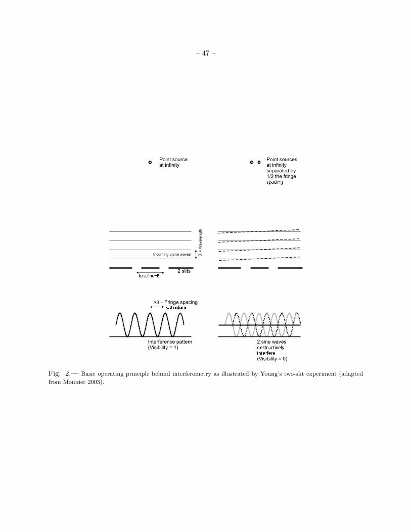
– 47 –

Fig. 2.— Basic operating principle behind interferometry as illustrated by Young’s two-slit experiment (adapted

from Monnier 2003).

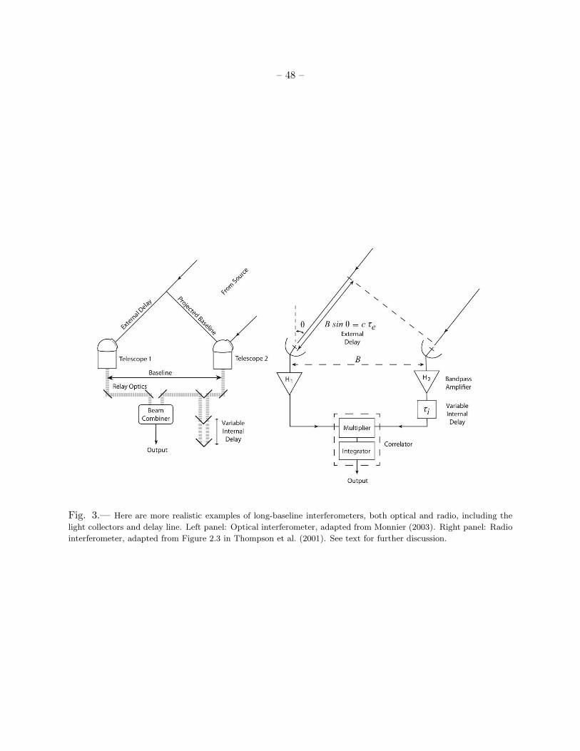
– 48 –

Fig. 3.— Here are more realistic examples of long-baseline interferometers, both optical and radio, including the

light collectors and delay line. Left panel: Optical interferometer, adapted from Monnier (2003). Right panel: Radio

interferometer, adapted from Figure 2.3 in Thompson et al. (2001). See text for further discussion.

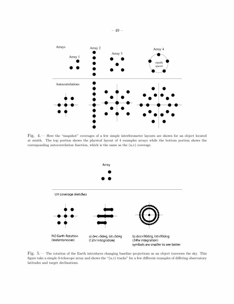
– 49 –

Array 3

Array 4

equally

spaced

Array 2

Array 1

Arrays

Autocorrelations

Fig. 4.— Here the “snapshot” coverages of a few simple interferometer layouts are shown for an object located

at zenith. The top portion shows the physical layout of 4 examples arrays while the bottom portion shows the

corresponding autocorrelation function, which is the same as the (u,v) coverage.

Fig. 5.— The rotation of the Earth introduces changing baseline projections as an object traverses the sky. This

figure take a simple 3-telescope array and shows the “(u,v) tracks” for a few different examples of differing observatory

latitudes and target declinations.

– 50 –

!"#$%&'#("%)##'$%

*+%,"-"./01".!

"2345%

67)8)%)##'$%

9%,"-"./01".!

"2345%

Fig. 6.— This figure shows the dramatic advantage in Fourier coverage that the Very Large Array (VLA) possesses

(left panel) compared to the CHARA array (right panel). The radio interferometer VLA, located in Socorro, NM, has

27 (movable) elements and the coverage shown here corresponds to observations ± 4.5 hours around source transit

(adapted from Thompson et al. 1980). The optical interferometer CHARA, located on Mt. Wilson, CA, has 6 (fixed)

elements and the coverage shown here corresponds to ±3 hours from transit (adapted from ten Brummelaar et al.

2005). The large gaps in Fourier coverage for CHARA limit its ability to reconstruct highly complex images.

– 51 –

Example Data Calibration

8.0 8.5 9.0 9.5 10.0Time (Hours)

0.0

0.2

0.4

0.6

0.8

1.0

1.2

Am

plitu

de (

arbi

trar

y)

Calibrator Target Calibrator Target Calibrator

8.0 8.5 9.0 9.5 10.0Time (Hours)

-3

-2

-1

0

1

2

3

Raw

Pha

se (

radi

ans)

Calibrator Target Calibrator Target Calibrator

Fig. 7.— First Step of Data Reduction

– 52 –

Calibrated Visibility

8.0 8.5 9.0 9.5 10.0Time (Hours)

0

10

20

30

40

Cor

rela

ted

Flu

x (m

illi-J

ansk

y)

Calibrator Target Calibrator Target Calibrator

8.0 8.5 9.0 9.5 10.0Time (Hours)

-3

-2

-1

0

1

2

3

Pha

se (

radi

ans)

Calibrator Target Calibrator Target Calibrator

Fig. 8.— Calibrator data following estimate of time-varying system visibilites.

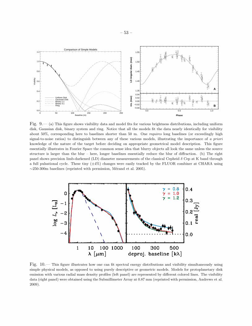
– 53 –

Comparison of Simple Models

0 50 100 150 200 250Baseline (m)

0.0

0.2

0.4

0.6

0.8

1.0

1.2

Vis

ibili

ty

Uniform DiskGaussian DiskBinary 1:1Binary 3:1Ring

A

0.0 0.5 1.0

1.35

1.40

1.45

1.50

1.55

B

0.0 0.5 1.0−0.04

−0.02

0.00

0.02

0.04

LD

An

gu

lar

dia

m. (

mas

)

Phase

res.

(m

as)

Fig. 9.— (a) This figure shows visibility data and model fits for various brightness distributions, including uniform

disk, Gaussian disk, binary system and ring. Notice that all the models fit the data nearly identically for visibility

about 50%, corresponding here to baselines shorter than 50 m. One requires long baselines (or exceedingly high

signal-to-noise ratios) to distinguish between any of these various models, illustrating the importance of a priori

knowledge of the nature of the target before deciding on appropriate geometrical model description. This figure

essentially illustrates in Fourier Space the common sense idea that blurry objects all look the same unless the source

structure is larger than the blur – here, longer baselines essentially reduce the blur of diffraction. (b) The right

panel shows precision limb-darkened (LD) diameter measurements of the classical Cepheid δ Cep at K band through

a full pulsational cycle. These tiny (±4%) changes were easily tracked by the FLUOR combiner at CHARA using

∼250-300m baselines (reprinted with permission, Merand et al. 2005).

Fig. 10.— This figure illustrates how one can fit spectral energy distributions and visibility simultaneously using

simple physical models, as opposed to using purely descriptive or geometric models. Models for protoplanetary disk

emission with various radial mass density profiles (left panel) are represented by different colored lines. The visibility

data (right panel) were obtained using the Submillimeter Array at 0.87 mm (reprinted with permission, Andrews et al.

2009).

– 54 –

1000 500 0 -500 -1000U coordinate (meters)

-1000

-500

0

500

1000

V c

oord

inat

e (m

eter

s)

Example uv coverage (6 antennas)

20 10 0 -10 -20Arcseconds (east)

0

50

100

150

Arc

seco

nds

(Nor

th)

Dirty Beam

20 10 0 -10 -20Arcseconds (east)

0

50

100

150

Arc

seco

nds

(Nor

th)

Dirty Map (for Binary)

Fig. 11.— The basic elements of the CLEAN algorithm consists of (a) the (u,v) coverage of the observations, (b)

the Dirty beam made from the Fourier Transform of the gridded (u,v) support, and (c) the Dirty Map made from

Fourier Transform of the observed (u,v) plane.

20 10 0 -10 -20Arcseconds (east)

-20

-10

0

10

20

Arc

seco

nds

(Nor

th)

Gridded Locationsof Clean Components

20 10 0 -10 -20Arcseconds (east)

-20

-10

0

10

20

Arc

seco

nds

(Nor

th)

Clean Beamfor Convolving

20 10 0 -10 -20Arcseconds (east)

-20

-10

0

10

20

Arc

seco

nds

(Nor

th)

Cleaned Map(without residuals)

Fig. 12.— The basic “restoration” steps of the CLEAN algorithm consist of (a) collecting the locations of the

CLEAN components, (b) creating a CLEAN beam which is a Gaussian beam with same angular resolution of the

central portion of the Dirty Beam, and (c) convolving the CLEAN components with the CLEAN beam. Here, the

final step of adding back the residuals of the dirty map has been left off. The arrows in panel (a) mark the location

of the two clusters of clean components near the locations of the two components of the binary.

– 55 –

Incoming plane waves

Point sourceat infinity

∆φ

∆φ

!

"#$#%&'(#!)

"#$#%&'(#!*

+',-&#

from

sourc

e

from

sourc

e

from

sourc

e

"#$#%&'(#!.

/'&0#1%!'2

34-5!46-!&4,%#

'(16&4$!(74%#

8#$49%

:$'%,-#

/74%#

"-64;<$#

Fig. 13.— (left) Atmospheric turbulence introduces extra path length fluctuations that induce

fringe phase shifts. At optical wavelengths, these phase shifts vary by many radians over short

time scales (<<1 sec) effectively scrambling the Fourier phase information. (right) Phase errors

introduced at any telescope causes equal but opposite phase shifts in ajoining baselines, canceling

out in the closure phase (see also Readhead et al. 1988; Monnier et al. 2006). (figures reprinted

from Monnier 2003)

– 56 –

Interferometer Facility Overview

10-2 100 102 104

Wavelength (mm)

0.0001

0.0010

0.0100

0.1000

1.0000

10.0000

100.0000

Max

imum

Ang

ular

Res

olut

ion

(arc

seco

nds)

NPOI

SUSI

CHARAVLT

I

VLTI

Keck-I

Keck-I

LBTI IS

I

ALMA

SMACARMAPdB

VLBA

eMERLIN

EVN

VERA

ATCA

EVLA

WSRT

DRAO

GMRT

MOST

LOFAR

1 m

icro

n

1 m

illim

eter

1 m

icro

n

1 m

eter

1 milli-arcsecond

1 arcsecond

1 arc-minute

Fig. 14.— Graphical representation of the wavelength coverage and maximum angular resolution

available using the radio and optical interferometers of the world. See Table 5 for more information.