radiation transfer model intercomparison (rami) exercise · radiation transfer model...

Radiation transfer model intercomparison (RAMI) exercise

Bernard Pinty,1 Nadine Gobron,1 Jean-Luc Widlowski,1 Sigfried A. W. Gerstl,1Michel M. Verstraete,1 Mauro Antunes,2 Cedric Bacour,3 Ferran Gascon,4 Jean-Philippe Gastellu,4 Narendra Goel,5 Stephane Jacquemoud,3 Peter North,6Wenhan Qin,7 and Richard Thompson8

Abstract. The community involved in modeling radiation transfer over terrestrial surfacesdesigned and implemented the first phase of a radiation transfer model intercomparison(RAMI) exercise. This paper discusses the rationale and motivation for this endeavor,presents the intercomparison protocol as well as the evaluation procedures, and describesthe principal results. Participants were asked to simulate the transfer of radiation for avariety of precisely defined terrestrial environments and illumination conditions. Thesewere abstractions of typical terrestrial systems and included both homogeneous andheterogeneous scenes. The differences between the results generated by eight differentmodels, including both one-dimensional and three-dimensional approaches, were thendocumented and analyzed. RAMI proposed a protocol to quantitatively assess theconsequences of the model discrepancies with respect to application, such as thosemotivating the development of physically based inversion procedures. This first phase ofmodel intercomparison has already proved useful in assessing the ability of the modelingcommunity to generate similar radiation fields despite the large panoply of models thatwere tested. A detailed analysis of the results also permitted to identify apparent“outliers” and their main deficiencies. Future undertakings in this intercomparisonframework must be oriented toward an expansion of RAMI into other and more complexgeophysical systems as well as the focusing on actual inverse problems.

1. Introduction

The primary goal of remote sensing research is to establishthe existence and nature of the formal relations between theradiative data collected on board of space platforms and thevariables of interest for the given applications. These radiativedata are controlled by the state variables of the radiation trans-fer problem, i.e., the smallest set of fundamental quantitiesrequired to fully describe the radiation transfer regime in thegeophysical media and not exclusively by the variables of in-terest [e.g., Verstraete et al., 1996]. The physical representationof the radiation transfer regime into geophysical media and atits geophysical boundaries is expressed in radiation transfer(RT) models. Any interpretation of satellite data relies onperforming the inversion of a model against a data string;models can be conceptual, empirical, or based on the mathe-

matical representation of the physics underpinning radiationtransfer as implemented into RT models. RT models thereforeconstitute an essential component for the quantitative inter-pretation of remote sensing data and the accuracy and reliabil-ity of the solutions to the inverse problems are determined bythe performance of both RT models and remote sensing in-struments.

In response to scientific questions and recent technologicaldevelopments, all major Space Agencies have invested sizableresources to design and implement a new generation of EarthObservation platforms and sensors to monitor adequately theland surface properties [e.g., Diner et al., 1999]. The upcomingavailability of such advanced instruments has, in turn, moti-vated significant algorithmic development and sophisticationwhich capitalizes on the improvements, made during the lastdecades by the RT community, in understanding the interac-tion between the solar radiation and the land surfaces (see, forexample, the review papers by Goel [1988] and Pinty and Ver-straete [1997]). Technological advances in aerospace and com-puter technologies allow the acquisition of data under muchbetter defined observation protocols, and recent theoreticaland simulation achievements should permit to take better ad-vantage of these new measurements [see Verstraete et al., 2000].By the same token, the full and proper interpretation of thesenew data sets will be better assessed to the extent that intrinsicuncertainties of the RT models are evaluated and further de-creased. The achievement of this goal requires an assessmentof, at least, (1) their relative performances via an intercom-parison exercise and (2) their accuracy and reliability in simu-lating well-documented in situ measurements of RT fields.

This paper describes the purpose and methodology of theradiation transfer model intercomparison (RAMI) exercise

1Global Vegetation Monitoring Unit, SAI-EC Joint Research Cen-tre, Ispra, Italy.

2Instituto Nacional de Pesquisas Espaciais, Sao Jose dos Campos,Sao Paulo, Brazil.

3Laboratoire Environnement et Developpement, Universite Paris 7,Paris, France.

4Centre d’Etudes Spatiales de la Biosphere, Toulouse, France.5Department of Computer Science, Wayne State University, De-

troit, Michigan.6NERC Centre for Ecology and Hydrology, Monks Wood, United

Kingdom.7NASA Goddard Space Flight Center, Atmospheric Chemistry and

Dynamics, Greenbelt, Maryland.8Alachua Research Institute, Alachua, Florida.

Copyright 2001 by the American Geophysical Union.

Paper number 2000JD900493.0148-0227/01/2000JD900493$09.00

JOURNAL OF GEOPHYSICAL RESEARCH, VOL. 106, NO. D11, PAGES 11,937–11,956, JUNE 16, 2001

11,937

Plate 1. Artist views of the RAMI scenes for discrete (a) homogeneous and (b) heterogeneous scenes.

PINTY ET AL.: RADIATION TRANSFER MODEL INTERCOMPARISON11,938

Plate 2. Illustration of the intercomparison strategy concept adopted in the RAMI exercise. The left panelsshow differences in BRF fields that can be produced by various idealized models, the middle panels give thehistograms of the local deviations (in percent) for every model, and the right panels indicate the correspondingvalues of the global deviation (in percent).

11,939PINTY ET AL.: RADIATION TRANSFER MODEL INTERCOMPARISON

(Historically, the remote sensing community had already per-formed a “model cook-off” in the mid-1980s when the firstcomputer models were tested for their usefulness in the inter-pretation of remote sensing data (N. Goel and F. Hall, privatecommunication, 1999.)) and outlines the results achieved sofar. This initiative constituted a key part of the preparation forthe “Second International Workshop on Multiangular Mea-surements and Models (IWMMM-2)” held at the Joint Re-search Centre (JRC) (Ispra, Italy) on September 15–17, 1999,where the results were first presented publicly. This intercom-parison has been set up by mid-June 1999 as a self-organizedactivity of the RT modeling community to which any partici-pants can contribute freely and can also derive its benefits. Theaim of RAMI is to focus on the performance of the RT modelsas an ensemble and to document the current uncertainties/errors among existing models in order to establish a consensusamong the surface RT modeling community. Such a modelintercomparison exercise also provides, in direct mode, bench-mark cases and solutions useful in the development and testingof RT models. In the longer term, it establishes a baselineprotocol against which further model improvements and de-velopments can be made. The extended results of this firstRAMI phase are available on the World Wide Web at thefollowing address: http://www.enamors.org/. Further exercisesand new results will continue to use this site for the foreseeablefuture.

2. Presentation of the RAMI ExerciseA wide variety of radiation transfer models have been de-

signed and published in the literature over the past decades.These operate at different levels of sophistication and arecapable of representing one-dimensional or three-dimensionaleffects, at quite different computational costs. Not all of thesemodels can easily be implemented in practical applications. Atthe same time, a sizable majority of users of remote sensingdata still use rather empirical tools, such as vegetation indices,in a wide variety of applications. In addition, multiangularmeasurements are becoming available from space platforms.The full exploitation of these data requires physically basedalgorithms based on RT models, which are the only tools

providing the necessary links between the observed fields andthe state variables of the target of interest.

A variety of questions could be envisaged in this context. Isthe objective solely to “fit” the observed reflectance field, withthe understanding that the physics of RT may or may not beproperly represented, or do we also require that the relation-ship between the state variables of the target of interest andthe observed reflectance fields are correctly and accuratelydescribed? In this latter case, what source of information couldserve as the reference or “truth” against which to evaluate therelative performance of the ensemble of models developed bythe community?

To advance along those lines, it was proposed to conduct aformal intercomparison exercise where a representative set ofmodels would be run in strictly defined configurations, to allowthe comparison of their results. Specifically, we have suggesteda two-pronged approach. First, we have proposed a series ofexperiments in direct mode, where each model is required tosimulate the transfer of radiation in precisely defined geophysi-cal scenes. The second and complementary experiment con-sists in providing a set of spectral and directional reflectancesand to require the models to provide their best estimates as tothe nature, structure, and properties of the scenes that couldhave generated such fields.

The overall objectives of this exercise are thus as follows: (1)to help developers improve their models, (2) to provide arationale for the acquisition of more or better data, (3) toprogressively develop a community consensus on the best waysto simulate the transfer of radiation at and near the Earth’ssurface, or on the optimal ways to exploit remote sensing data,and (4) to inform the user community on the performance ofthe various models available.

The following sections describe the experimental protocol indirect mode. Precisely defined scenes containing idealized soilsand vegetation canopies are described in such a way that themodels available can represent the spectral and directionalreflectance fields of these targets, and a well-defined method-ology is set up to compare the results as an ensemble. A similarexercise in inverse mode has also been proposed, but very fewresults have been submitted at the time of writing.

Table 1. List of RAMI Models, References, and Participants

Model Type Model Name Reference Participant

1-D ProSAIL Verhoef [1984] andJacquemoud and Baret [1990]

C. Bacoura andS. Jacquemouda

homogeneous ProKuusk Kuusk [1995] andJacquemoud and Baret [1990]

C. Bacour andS. Jacquemoud

scenes 1/2 Discrete Gobron et al. [1997] N. Gobronb

3-D Flight North [1996] P. Northc

heterogeneous DART Gastellu-Etchegorry et al. [1996] F. Gascond andJ.-P. Gastellud

scenes Sprint Thompson and Goel [1998] R. Thompsone

and N. GoelfRAYTRAN Govaerts and Verstraete [1998] J.-L. WidlowskibRGM Qin and Gerstl [1999] W. Qing

aLaboratoire Environnement et Developpement.bJoint Research Centre.cNatural Environment Research Council.dCentre d’Etudes Spatiales de la Biosphere.eAlachua Research Institute.fWayne State University.gGoddard Space Flight Center.


2.1. RAMI ProtocolThe RAMI protocol was designed around a limited set of

modeling exercises for both homogeneous and heterogeneousgeophysical conditions or scenes. These have been selected torepresent a broad set of well-defined remote sensing problemsfor which the solutions can be easily compared. They obviouslydo not pretend to cover the full range of experiments thatwould be required to fully document all aspects of modelperformances. Rather, we focused on a limited but still com-putationally demanding set of basic cases appropriate to fulfillthe initial objectives of RAMI.

For all proposed experiments the participants were encour-aged to produce, in addition to the total spectral BRF values,the corresponding contributions due to the uncollided radia-tion by the leaves, the singly collided by the leaves, the radia-tion multiply collided by the leaves, and the soil, in both theprincipal and the cross planes. Additional quantities, includingthe spectral albedo of the canopy, i.e., the directional hemi-spheral reflectance, and the absorption of radiation in thevegetation layer were also asked for. In the case of the heter-ogenous scenes, a set of additional diagnostic parameters werealso established to help in understanding the origins of anypotential discrepancies between the model results. The fulldocumentation on the experimental protocol for all the pro-posed simulations can be found at the following World WideWeb address: http://www.enamors.org/. RAMI was conceivedas a free exercise to which anybody could contribute and, as anexample, any user of a published model could run its ownand/or other versions of the same code provided elsewhere.Table 1 lists the RAMI models and the corresponding publi-cation in the peer-reviewed literature documenting these mod-els and, finally, the participant names and affiliations.

2.1.1. Homogeneous scenes. As illustrated in Plate 1a,homogeneous scenes are made up of (1) randomly distributedscatterers with anisotropic scattering functions to be treated asa turbid medium (e.g., oriented point-like scatterers) and (2)randomly distributed finite-size scatterers (e.g., equivalent toleaves) with anisotropic scattering properties. The RT problemto be faced for these homogeneous scenes can be solved eitherusing one-dimensional or three-dimensional models. These se-ries of experiments thus permit us to intercompare the perfor-mances of models delivering one-dimensional solutions be-

tween themselves and also against those given by the morecomplex models that solve explicitly the RT equation in thethree spatial dimensions.

Tables 2, 3 and 4 summarize the input values for the illumi-nation and viewing geometries, the architectural variable val-ues, and the spectrally dependent values, respectively, to beused for the proposed simulations.

A variety of combinations of these state variable values havebeen used to simulate the bidirectional reflectance factor(BRF) fields at red and near-infrared wavelengths which aretwo spectral regions of importance for land surface remotesensing due to the typical signature of green leaves.

Additional sets of exercises have been proposed to verifymodel compliance with energy conservation and to benchmarkthe more complex models against those providing quasi-analytical solutions under particular circumstances. These setsare designed to simulate the radiation transfer regime forhomogeneous scenes with conservative scattering conditions.In these cases the scatterer reflectance and transmittance val-ues are both equal to 0.5, and the soil reflectance is equal to1.0. The additional variables are at fixed values equal to 0.1 mfor the leaf diameter, 1.0 m2/m2 for the leaf area index, and1.0 m for the height of the canopy, respectively. Two leaf angledistribution functions, namely erectophile and planophile, aresuggested for performing the simulations at three differentillumination zenith angles, i.e., 0!, 30!, and 60!.

2.1.2. Heterogeneous scenes. Plate 1b exhibits a repre-sentation of the heterogenous scenes made up of randomlydistributed spherical envelopes of finite size that contain eitherfinite-size randomly distributed elements or quasi-turbid me-dium. The experiments were designed for models able to pro-vide solutions to the full three-dimensional radiative transferproblem using a variety of approaches relying on ray-tracingtechniques, computer graphics, and three-dimensional spacesolutions of the RT equation. Each individual scene is com-posed of a horizontal plane featuring the background soil and

Table 2. Variables Defining the Illumination and ViewingGeometries

Symbol Variable Values

!0 source zenith angle 20! and 50!!v view zenith angle from 0! to 70!

in step of 2!" relative azimuth angle 0! and 180!

Table 3. Variables Defining the Structure of HomogeneousScenes

Variable Identification Values

Leaf area index (LAI) 3 m2/m2

Height of the canopy 2.0 mEquivalent leaf diameter infinitely small, 0.1

and 0.2 mLeaf angle distribution erectophile and planophile

Table 4. Variables Defining the Spectral Leaf and SoilProperties

Variable IdentificationRed

ValuesNear-Infrared

Values

Leaf reflectancea 0.0546 0.4957Leaf transmittancea 0.0149 0.4409Soil albedob 0.1270 0.1590

aUsing a bi-Lambertian scattering law.bUsing a Lambertian scattering law.

Table 5. Variables Defining the Structure ofHeterogeneous Scenes

Variable Identification Values

Leaf shape Circular disk ofnegligible thickness

Leaf diameter infinitely smalland 0.2 m

Leaf area index of a sphere 5 m2/m2

Leaf angle distribution uniformNumber of spheres 15Sphere radius 10 mRange of sphere center height from 11 to 19 mFractional sphere area coverage 0.471


a number of nonoverlapping disk-shaped scatterers whose nor-mals follow a uniform distribution. The scatterers are confinedwithin large spherical bodies distributed randomly across thescene at various heights. The spectral properties of the indi-vidual elements composing the scenes as well as the illumina-tion and viewing conditions are identical to those specified inTables 4 and 2, respectively. Table 5 provides the values of thekey architectural variables specifically used for the scenes.

2.2. Evaluation StrategyThe intercomparison of model results raises a number of

fundamental issues and outstanding problems related to thenotion of absolute truth and model verification/validation.Such issues have long been debated in all generality by thebroad scientific community; an overview of the problems to beaddressed in the context of Earth sciences is presented byOreskes et al. [1994]. This contribution provides elements tosupport the conclusion that the model results cannot be com-pared against an absolute reference per se which would be theactual “truth” simply because the latter cannot be established.As such, this statement implies that an absolute “model veri-fication” is impossible. Therefore rather than looking for the“truth,” the analysis of the ensemble of model results is

achieved such that it yields the establishment of the “mostcredible solutions” as a surrogate for the “truth.” Although itis tempting to derive this surrogate from the estimation of thevarious moments of the distributions of model results, it mustbe recognized that for instance, model deviations with respectto an ensemble arithmetic average are difficult to interpret inthe presence of potential “outliers” that could bias this esti-mation. Given an ensemble of model results, it is, however,feasible to compare the model results against each other inorder to document their relative differences: this is the primaryintent of RAMI.

The primary criterion to quantify intermodel variabilitywithin the context of RAMI is a measure of distance betweenBRF fields generated under identical geophysical and geomet-rical conditions. Specifically, the following metric is computedto estimate how a given model behaves with respect to anensemble of models:#m"!v#

$1! !

i$1

N!0 !s$1

Nscenes !%$1

N% !k$1,k%m

Nmodels "&m"!v, i , s , %# & &k"!v, i , s , %# "&m"!v, i , s , %# ' &k"!v, i , s , %#

(1)

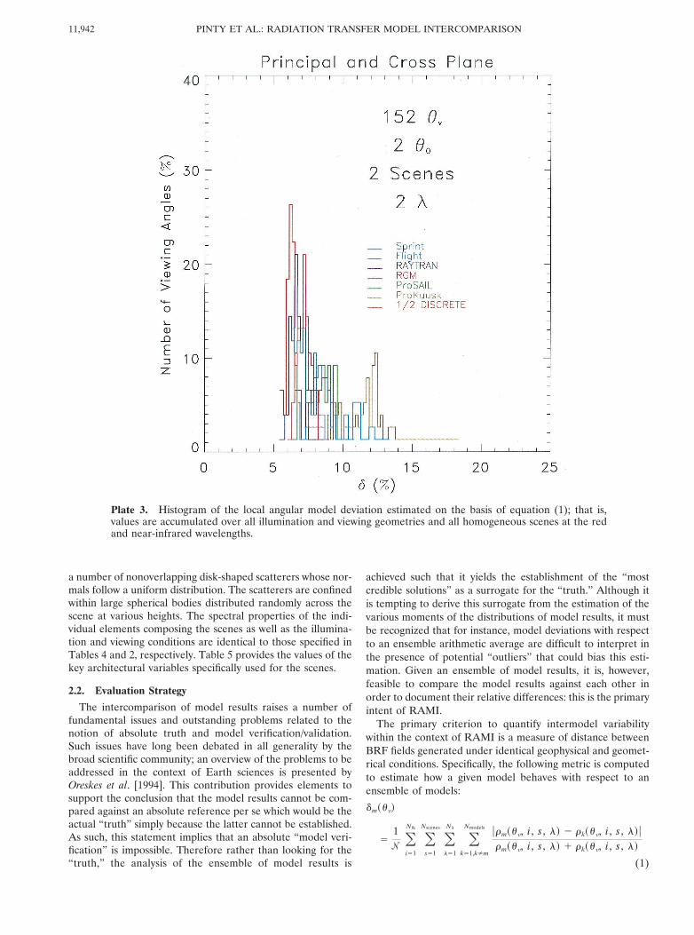
Plate 3. Histogram of the local angular model deviation estimated on the basis of equation (1); that is,values are accumulated over all illumination and viewing geometries and all homogeneous scenes at the redand near-infrared wavelengths.


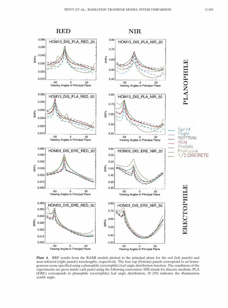
Plate 4. BRF results from the RAMI models plotted in the principal plane for the red (left panels) andnear-infrared (right panels) wavelengths, respectively. The four top (bottom) panels correspond to an homo-geneous scene specified using a planophile (erectophile) leaf angle distribution function. The conditions of theexperiments are given inside each panel using the following convention: DIS stands for discrete medium, PLA(ERE) corresponds to planophile (erectophile) leaf angle distribution, 20 (50) indicates the illuminationzenith angle.


where #m(!v) expresses local angular deviation of model m atthe specific exiting angle !v with respect to the ensemble ofNmodels models. This deviation, normalized by the number ofcases considered (!) is estimated for all simulations of theBRF fields, emerging from Nscenes at N% wavelengths, illumi-nated with N!0

incident source angles; &m(!v, i , s , %) and&k(!v, i , s , %) correspond to the BRF values generated bymodel m and any other RAMI model k participating in theexperiment, respectively.

Similar metrics can be designed to examine the model dis-crepancies for each geometrical condition of illuminationand/or observation, scene, and wavelength. They can all bederived following the generic form of (1). For instance, theappropriate metric for analyzing the model discrepancies sep-arately for each wavelength would be

#m"!v, %#

$1! !

i$1

N!0 !s$1

Nscenes !k$1,k%m

Nmodels "&m"!v, i , s , %# ' &k"!v, i , s , %# "&m"!v, i , s , %# ( &k"!v, i , s , %#

.

(2)

Alternatively, (1) can also be ultimately integrated over allavailable viewing conditions to estimate a global angular modeldeviation:

#m $1

N!v

!l$1

N!v

#m"!v# , (3)

where #m denotes a global deviation of the model that resultsfrom an estimation of the sum of the local deviations estimatedat each and every exiting angle on the basis of the metricexpressed by (1).

For the sake of explanation, Plate 2 illustrates the behaviorof the measures of the local and global angular deviations inidealized cases. These are based on very simple model resultssuch as those corresponding to a Lambertian medium andperfectly bowl-shaped reflectance fields. This conceptual exer-cise illustrates that (1) the values of the metrics defined by (1)and (3) depend on the number of RT models entering theintercomparison exercise and (2) the larger the number ofmodels that produce similar BRF fields, the smaller the valuesestimated by the two metrics. Indeed, the intercomparison ofresults from two RT models only (top panels) produces ratherflat histograms of the local deviation and, obviously, identicalglobal deviation values. The addition of one more model (mid-dle panels), generating BRF fields different from the twoformer models, draws local deviation values closer to zero butthe presence of “outliers” is difficult to assess. In this case, theglobal deviation metric would slightly favor the Lambertianmodel (red color) in the sense that it deviates less from theother two. However, when a fourth RT model, generating BRFfields very close to at least one of the former models, is intro-duced for evaluation (bottom panels), the histograms of thelocal deviations are significantly narrowed and these similarRT models are more easily identified within the full set on thebasis of the global deviation metric by producing lower #m

values than the others.In summary, it is worthy to note that as desired in the context

of the community effort to assess the state of the art of itsmodels, (1) the larger the number of participating models, theeasier the identification of “outliers” if any, (2) the agreement

between the BRF fields produced by many models permitidentifying them as being able to generate the “most crediblesolutions.”

From the perspective of analyzing the model intercompari-son results, it appears that (1) the global deviation metricprovides an overall estimation of the model discrepancies, (2)the envelope of the histograms of the local deviation metricvalues permits to assess the various modes of the distributionof these model discrepancies, and (3) the joint analysis of theindividual histograms of the local deviations for every modelpermits to quantify its behavior against the others. As statedabove, any simple statistical analysis tends to favor the subsetof models generating the most analogous results. However, inthe absence of the absolute “truth,” there are no definite rea-sons to exclude “outliers” on the sole basis of the statisticalanalyses. An inspection of the physics underlying the RT mod-els and/or the implementation of these models is definitelymandatory to get a rationale regarding model deviations. Inpractice, the SAI/JRC research group has led the RAMI ex-ercise and has ensured contacts with the participants specifi-cally in case of doubtful results that could have revealed somemodel implementation errors. This first phase of RAMI wasperformed blindly by the participants in the sense that they didnot know a priori who else was participating, which modelswere used, and which experiments were made.

3. Overview of RAMI ResultsThe participants in RAMI performed a large number of

radiation transfer computations. These were analyzed and arather exhaustive set of results is available at the followingWorld Wide Web address: http://www.enamors.org/. This sec-tion highlights the most prominent results (The figures anddiagrams shown here are built on all results available by end ofAugust 1999.) for the RT modeling and general scientific com-munity.

3.1. Homogeneous ScenesFigure 1 shows a series of histograms of local angular model

deviation values estimated for viewing conditions in the prin-cipal plane (left panels), cross plane (middle panels), and theprincipal and cross planes together (right panels). The top,middle, and bottom panels display the results obtained at thered, the near-infrared, and at the red and near-infrared wave-lengths together, respectively. As such, this figure demon-strates the large spread of results delivered by a set of sevenBRF models (all models listed in Table 1, but DART, per-formed the experiments suggested for the homogeneousscenes) representative of the community modeling capacity.Almost all graphs reveal the presence of a first well-markedpeak extending from about 8 to 12% and 3 to 6% at the redand near-infrared wavelengths, respectively, and a secondpeak, less intense close to 15% at the red wavelength. Therelative increase in model discrepancies at the red wavelengthrepresents, presumably, the diversity of approaches to addressthe fundamental plant canopy specific issue of leaf size effects.The values obtained when estimating the local model deviationat the near-infrared wavelength reflects mainly the differencein the methods used to estimate the multiple-scattering com-ponents in the plant-soil system.

The panel located at the bottom right of Figure 1 summa-rizes the values of the local angular deviations when summedup over the two wavelengths and viewing planes. The bimodal


nature of this histogram indicates the presence of one or more“outliers” in the sense discussed in section 2.1; that is, theyproduce BRF values that are distinctly different from thosedelivered by the other RAMI models. A detailed inspection ofthese results reveal that for all cases examined in Figure 1, twoRAMI models are producing the secondary peak. Plate 3 iden-tifies the individual behavior of all RAMI models and revealsthat in a statistical sense, both ProKuusk and Flight modelsdeviate the most from the other models.

Plates 4 and 5 exhibit the BRF results delivered by theRAMI models in the principal and cross planes, respectively.Overall, it can be seen that the models show relatively moredisagreement between themselves in simulating the planophilecanopy conditions. Indeed, in the erectophile case (four bot-tom panels), only ProKuusk and ProSAIL produce a relativelylarge backward regime and simulate an angularly larger hotspot than is the case for the other models. The Flight modeldiffers slightly from the other models in generating globallylower BRF values. This difference has been traced to an errorin computing the single-scattering phase function, which hassince been corrected. Less systematic but still large deviationsare produced by ProKuusk in mostly all cases, and additionalpeaks can be detected both in the principal and in the crossplanes outside the hot spot region. The latter are due to theleaf specular reflectance as implemented in the original

Kuusk’s model. Plates 4 and 5 show clearly that major modeldiscrepancies are occurring in backward conditions and espe-cially within a relatively large solid angle embedding the hotspot effect. It should also be noted, however, that the variousimplementation of the erectophile and planophile leaf angledistribution functions could have lead to some differences inthe model results.

The model discrepancies naturally translate into major an-gularly integrated quantities such as the absorption and thealbedo for direct illumination, i.e., the directional hemispher-ical reflectance. The results shown in Figures 2 and 3 demon-strate that quite significant variability can be obtained in thecase of a planophile leaf angle distribution function. It must berecalled here that the three-dimensional models estimate theintegrated quantities in different manners, depending, for in-stance, on whether they use a direct or inverse Monte Carlotracing technique.

3.2. Heterogeneous Scenes

Plate 6 shows the histogram of the local angular modeldeviations estimated by (1), i.e., summed up over the twowavelengths and viewing planes, on the basis of four concep-tually different three-dimensional models. It can be seen thatthe values range from 3 to 6% and that only one model(DART) contributes to the secondary peak at the largest ob-

Figure 1. Histograms of local angular model deviations estimated for viewing conditions in the principalplane (left panels), cross plane (middle panels), and the principal and cross planes together (right panels). Thetop, middle, and bottom panels display the results obtained at red, near-infrared, and red and near-infraredwavelengths together, respectively. All results are obtained using the conditions given in Tables 1, 2, and 3 forthe homogeneous scenes.


Plate 5. Same as Plate 4 except in the cross plane.


served deviation values. This specific behavior is particularlysignificant at the near-infrared wavelength and additional re-sults from RAMI show that this is due to a 10% underestimateby DART of the multiple-scattering estimates of the otherthree models.

Plates 7 and 8 show that indeed for both viewing planes, agood agreement between the three-dimensional models is ob-tained despite the large dynamic range in the simulated BRFfields. The top four panels of these figures correspond to re-sults obtained in the case of a heterogeneous scene where thespheres are filled up with leaves of 0.2 m diameter producinga well-marked peak in the backscattering region. The bottompanels exhibit BRF fields produced by the same large-scalearchitecture but for turbid media spheres, i.e., made up of avery large number of point-like oriented (infinitely small) scat-terers. In these latter cases the excellent agreement between allthree participating models is quite noticeable, in particular, forthe representation of the backscattering enhancement con-trolled by the large-scale voids between the spheres. This isremarkable since the turbid spheres may still be represented bysmall, yet finite-size scatterers; that is, in the case ofRAYTRAN the leaf diameter is equal to 0.002 m.

These slight differences between the three-dimensional

model results do not translate into large variations in fluxquantities such as the spectral albedo and absorption factors,however, and an overestimate (underestimate) of albedo ismainly compensated by an underestimate (overestimate) of theabsorption factor.

3.3. Model Discernability

A well-designed BRF model intercomparison exerciseshould ideally yield practical indications on the ability of themodeling community to effectively simulate the reflectancefields of a variety of geophysical scenes. This can be done withdifferent tools, provided they represent the same “reality” innumerically acceptable ways. A common issue arising withinverse problems is the occurrence of multiple solutions, i.e., inthe present case, the possibility of defining multiple geophysi-cal scenarios that would be able to explain the observations.This situation arises because either there are not enough mea-surements, or the observations are not accurate enough toconstrain the numerical inversion process, or because the mod-els themselves are incorrect or incomplete. In any case thisissue becomes one of distinguishing between models that gen-

Plate 6. Histogram of the local angular model deviation estimated on the basis of equation (1); that is,values are accumulated over all illumination and viewing geometries and at the red and near-infraredwavelengths for the heterogeneous scenes.


erate different results on the basis of limited samples of im-perfect data.

To address this issue, it is necessary to develop an approachwhere the errors of measurements are somehow compared tothe variability exhibited by the different models in their rep-resentation of reality. A statistical measure of the joint behav-ior of these models in terms of their capability of representinga sample of data is thus proposed, and it will be seen that at agiven level of accuracy, some models cannot be distinguished,while others can be declared to behave differently. One con-sequence of this approach is that as measurements improve inaccuracy, the differences between models become more no-

ticeable. In a pragmatic sense, differences between RT modelsmatter only to the extent that they exceed the level of uncer-tainty associated with the measured BRF fields.

The absence of any absolute “truth” in the sense discussed insection 2.2 renders the exercise more tricky, but nevertheless,the model discernability issue can be addressed by assessingthe “most credible solutions.” As a matter of fact, it can rea-sonably be admitted that the latter correspond to the actualvalues that could be measured from an instrument with itsintrinsic limited accuracy. We attempted to examine the issueof model discernability taking advantage of the fact that atleast in the case of homogeneous scenes, both one-dimensional

Figure 2. Model results in estimating the spectral albedo, i.e., directional hemispherical reflectance, for thehomogeneous scenes at the red (left panels) and near-infrared (right panels) wavelengths. The informationprovided into each individual panel follows the convention given in Plate 4.


and three-dimensional models could be applied. Accordingly,we established for all scenarios what could be considered as the“most credible solutions” by estimating the arithmetic mean ofevery BRF value calculated within a subset of the three-dimensional model results. The model discernability can thenbe analyzed by comparing the values computed with the fol-lowing normalized )2 metric:

)2 $1! !

i$1

N!0 !j$1

N!v !s$1

Nscenes !%$1

N% (&"i , j , s , %# ' &Credible"i , j , s , %#)2

*2"%#,

(4)

with

&Credible"i , j , s , %# $ *&3D"i , j , s , %#+ , (5)

*3D2 "%# $

1NB ' 1 !

m$1

N3D !i$1

N!0 !j$1

N!v !s$1

Nscenes

(&3D"i , j , s , %#

' &Credible"i , j , s , %#)2. (6)

Equations (5) and (6) provide an estimate of the average ofthe NB BRF values taken over of a subset of N3D three-

Figure 3. Model results in estimating the spectral absorption factor for the homogeneous scenes at the red(left panels) and near-infrared (right panels) wavelengths. The information provided into each individualpanel follows the convention given in Plate 4.


Plate 7. BRF results from the RAMI models plotted in the principal plane for the red (left panels) andnear-infrared (right panels) wavelengths, respectively. The four top (bottom) panels correspond to a heter-ogenous scene specified using a large (extremely small) leaf diameter. The conditions of the experiments aregiven inside each panel using the following convention: DIS (TUR) stands for discrete (turbid) medium, UNIcorresponds to uniform leaf angle distribution, 20 (50) indicates the illumination zenith angle.


Plate 8. Same as Plate 7 except in the cross plane.


dimensional RAMI models and the associated value of thevariance of the BRF distribution of these latter models. ! is anorm equal to the number of available cases. In the presentanalysis of model discernability we excluded two of the fivethree-dimensional models that participated in RAMI: theDART and Flight models, which were shown to deviate themost for some of the proposed simulation scenarios. Finally,on the basis of the BRF values generated by the RGM, RAY-TRAN, and Sprint models we obtained *3D

2 (%) values of 1.6 ,10&3 and 1.0 , 10&2 at the red and near-infrared wavelengths,respectively. These values correspond approximately to 5%and 2% of the typical BRF values that can be measured overa plant canopy system at the red and near-infrared wave-lengths, respectively. Such values are within the expected rangeof those to be estimated from the upcoming multiangular datato be soon gathered in space.

The denominator of (4), *2(%) corresponds to the sum of thevariance associated to each individual model and the actualmeasurements [Kahn et al., 1997]. As a first attempt, we ap-proximate the value of *2(%) by simply considering that theuncertainties linked to the models are identical to those asso-ciated to the measurements:

*2"%# $ 2*3D2 "%# . (7)

The results of the application of the )2 metric defined by (4)are graphically shown in Figure 4. The vertical line at )2 $ 1.0defines two subspaces in the diagram. All models falling to theleft of this line (0 - )2 - 1.0) are indistinguishable on the basisof the available sample of measurements, while those thatstand on the right ()2 . 1.0) generate BRF fields statisticallydifferent at the prescribed level of error. In other words themodels located on the left of this line (RAYTRAN, RGM, 1/2Discrete and Sprint) are simulating BRF fields which are notsignificantly different, in the sense that the statistical differ-ences between their results cannot be considered meaningful.By contrast, the models Flight, ProSAIL, and ProKuusk do notrepresent correctly enough the BRF fields from an ensemble ofhomogeneous scenes. It can readily be foreseen that increasing(decreasing) the data and model accuracies, through the valueof the denominator in (4), would move the )2 $ 1.0 verticalline to the left-hand (right) side of the diagram, so the subset

of undiscernable models would become smaller (larger).Hence more accurate data will better help distinguish betweenmodels, and their effective interpretation may, in turn, requireimproved models.

Although this approach remains incomplete, we surmise thatthis type of RT model intercomparison analysis leads to con-crete pragmatic conclusions as far as models are concerned. Italso provides sound justification to acquire data with specificaccuracy and precision requirements. During this first phase ofRAMI, we limited the model discernability analysis to the caseof the homogenous scenes because here it is acceptable todefine the “most credible solutions” to the radiation transferproblem on the basis of the simulations done by three-dimensional models. The latter showed, however, a good levelof agreement in the case of heterogeneous scenes, admittingthat some accuracy can easily be gained in the simulation of themultiple-scattering regime by sacrificing more on the compu-tational performances of the code. It is a very encouragingoutcome of RAMI that these three-dimensional models arealmost equivalent, at least as far as the geophysical scenes westudied are concerned, and this despite the fact that they sharevery little in terms of approach, numerical methodology andimplementation techniques. In the future, better and addi-tional data, or a different set of scenes, may help to assess theirlimits of applicability, or confirm their correct representationof these measurements.

3.4. MiscellaneousA number of aspects related to RT modeling have been

touched by the RAMI exercise, including information aboutthe computational expenses of the codes, the capacity of ad-dressing a straightforward inverse problem and the verificationof model compliance with respect to energy conservation.

The information related to the computational requirementsare not reported here since they strongly depend on the codingskills of the programmer and the amount of effort spent incode optimization. In any case, software prototypes can alwaysbe tuned to a given platform. Ideally, the intercomparison ofmodel exploitation costs should be conducted under the samecomputational environment. However, even with these condi-tions, it will remain difficult to draw definite conclusions onthat matter since, as an example, some models may fully profitfrom specific hardware and software features such as vector-ization and parallelization. A dedicated protocol has to beestablished in order to address the issue of model computa-tional efficiency, as already suggested in the context of theIntercomparison of 3-D Radiation Codes (I3RC) initiative (in-formation about I3RC is available at the following World WideWeb address: http://www.i3rc.gsfc.nasa.gov).

The RAMI initiative also included inverse problems as partof its first phase. We specified two inverse problems where onlyBRF fields at the top of the canopy were given with the ob-jective of deriving as many biogeophysical parameters of thecanopy as possible from an inverse calculation. As in all real-world inverse problems, the solution is not unique because theproblem is ill-conditioned. Giving a full or even a partial BRFis equivalent to measuring radiances in different directionsabove a given scene. Clearly, such data from actual measure-ments have always uncertainties associated with them whichare characteristic of the instrument capabilities and often alsocontain the effects of atmospheric perturbations that cannot bewell defined or corrected for. Consequently, as a first step, weproposed only calculated BRFs without atmospheric effects. In

Figure 4. Plots of the )2 values estimated using equation (4)for each of the RAMI models in the case of the homogeneousscenes. The cross and diamond signs identify the one-dimensional and three-dimensional models, respectively.


this case, a specific forward model calculation has been used toproduce these BRFs with a particular set of model parameters,so the solution of the inverse problem is known by the researchteam leading the exercise. This set of model parameter valuesconstitutes the “true solution” of the problem. The inverseproblem therefore consists in finding one or more sets of vari-able values yielding BRF fields not statistically different fromthe “true” one with respect to the specified uncertainty. The“true solution” can thus be used as a standard for comparingthe results from the inverse calculations performed by theintercomparison participants. An additional exercise was de-fined with the provision of only nine BRF values along a slicethrough the full BRF distribution at red and near-infraredwavelengths; this more realistic case is taken to be some-what analogous to the situation that arises for measure-ments from the MISR instrument on the EOS-Terra plat-form. Although the specification of these inverse problemsoffered quite a range of possibilities for many participants(that is, classical vegetation indices can be applied as usuallydone with actual imperfect data from space), the inversemode received very little attention and only one participant(F. Gao (Boston University) applied its knowledge-baseduncertainty inversion technique.) outside the leading teamat JRC did propose some answers. Accordingly, these exercisesin inverse mode are still ongoing and should deserve moreattention in the future.

The verification of model compliance with respect to energyconservation was addressed on the basis of a set of conserva-tive scattering experiments, as explained in section 2.1. Thelarge computing time requested by some three-dimensionalmodels has been an issue to ensure the performance of thesesimulations using advanced tools. As a matter of fact, onlythree models, namely Flight, RAYTRAN, and 1/2 Discrete,have been tested against these academic conditions referringto finite-size scatterers. (Similar experiments were carried outfor turbid conditions in which Sprint also participated.) Plates9 and 10 illustrate the BRF fields simulated by these models inthe principal plane for erectophile and planophile leaf angledistribution functions, respectively. The overall agreement be-tween the three model results, especially when considering anerectophile leaf angle distribution function and the lowest leafarea index values, is quite impressive under such drastic scat-tering conditions. The differences in the simulated BRF resultsincrease almost systematically in the forward scattering direc-tion.

Having set up a pure conservative scattering experiment forhomogeneous media made up of finite-size-oriented scatterers,the theoretical albedo and absorption factor values are equalto 1.0 and 0.0, respectively. In all experiments, except in thecase of planophile canopy illuminated at 60! for which thesimulation results are not available, the RAYTRAN modelrecovers the theoretical values with a numerical accuracy ofabout 10-4. The 1/2 Discrete model delivers albedo and absorp-tion factor values which are off by 0.02 (0.045) absolute in theworst case using an erectophile (planophile) leaf angle distri-bution. These estimates are not available for other models, andstatistics can therefore not be established at this time, however,under standard scattering canopy conditions when measured atthe red and near-infrared wavelengths, the compliance withrespect to energy conservation should be satisfied to a muchhigher degree of accuracy than with respect to other processesat work.

4. Conclusions and PerspectivesThe modeling groups participating in the first phase of the

RAMI exercise constitute a significant fraction of the interna-tional community, and their models are representative of therange of existing radiation transfer models currently applied indirect and inverse mode. The RAMI initiative is set up as aself-organized and ongoing activity to which any researcher isfree to participate. This approach yields a documentation ofthe variability produced by the models currently in use in theRT modeling community. The first phase has already proveduseful in (1) quantifying the variability of BRFs simulated by alarge set of RT models under various geophysical scenarios, (2)pointing out some model discrepancies at large angles and inthe angular region where backscattering is enhanced by theleaf size effects, (3) benchmarking three-dimensional modelsimulations and verifying their numerical implementation, and(4) evaluating model discrepancies on the basis of a discern-ability concept in line with the use of these RT models in aninverse mode.

The overall impression left by inspecting the various resultsis that the modeling community has reached a high level ofmaturity because of its willingness to participate in such anexercise. Discrepancies are documented and linked to specificrequirements that can be translated into measurement require-ments. There are obviously a few specific areas where modelimprovements can be envisaged and certainly performed with-out facing significant difficulties. As a matter of fact, somemodel improvements have already been made by the partici-pants following the evaluation of the results obtained duringthe first phase of RAMI; an update of the improved modelresults will be presented during the second phase of the RAMIexercise where it is expected that the model variability in theangular domain will be reduced, at least for these specificcases. The full potential of this intercomparison exercise re-mains, however, to be exploited through a continuation of thisfirst RAMI phase. It is, for instance, important to have allparticipating models to perform all experiments in order tomake a more complete assessment of their relative capabilities.

With the benefit of the model intercomparison results ob-tained over simple geophysical scenarios, it can now be envis-aged to pursue this strategy by reinforcing the number andvariety of canopy conditions to be simulated. For instance, themonitoring and characterization of the boreal and, more spe-cifically, coniferous forests are of major importance for globaland regional climate modeling. However, none of the RAMIexperiments proposed in this first phase could actually copewith these biome types although some advanced and dedicatedmodels have long been developed [e.g., Li and Strahler, 1986;Li and Strahler, 1992; Peltoniemi, 1993; Li et al., 1995;Knyazikhin et al., 1997; Chen and Leblanc, 1997; Ni et al., 1998].

The RAMI results constitute a unique set of simulated BRFfields and a platform against which the improvements fromnew models, further model developments, and innovationcould be objectively assessed. We believe that this platform willstimulate scientific interactions and inform the community onthe state of the art at regular time interval. At the same time,we expect that these developments will both justify a posteriorithe investments already made to acquire more and better datawith laboratory, field, airborne and spaceborne instruments,and motivate the community to pursue further improvementsin this direction.


Plate 9. Plots of the BRFs simulated by the Flight (light blue curve), RAYTRAN (deep blue curve), and 1/2Discrete (red curve) models, in the principal plane for a homogeneous scene with an erectophile leaf angledistribution function. Other variable values are given in section 2.1.


Acknowledgments. The technical assistance of Gianni Napoli isgratefully acknowledged by the participants. The RAMI exercise wasconceived and implemented as part of the preparation for theIWMMM-2 conference jointly sponsored by (1) the European Net-work for the development of Advanced Models to interpret OpticalRemote Sensing (ENAMORS) data over terrestrial environments sup-ported by the DGXII under the Fourth Framework Programme, (2)the Space Applications Institute (SAI) of the JRC, (3) the NationalAeronautics and Space Administration (NASA), and (4) the Common-wealth Scientific and Industrial Research Organization (CSIRO). Thispaper benefited indirectly from progress achieved by other research

groups in geophysics which organized analogous intercomparison ex-ercises in the field of clouds and, more generally, atmospheric models.Mauro Antunes is supported by FAPESP. Many thanks to A. Kuuskwho sent C. Bacour and S. Jacquemoud the software code of hisMarkov chain model of canopy reflectance.

ReferencesChen, J. M., and S. G. Leblanc, A four-scale bidirectional reflectance

model based on canopy architecture, IEEE Trans. Geosci. RemoteSens., 35, 1316–1337, 1997.

Plate 10. Same as Plate 9 except for a planophile leaf angle distribution function.


Diner, D. J., G. P. Asner, R. Davies, Y. Knyazikhin, J.-P. Muller, A. W.Nolin, B. Pinty, C. B. Schaaf, and J. Stroeve, New directions in earthobserving: Scientific applications of multiangle remote sensing, Bull.Am. Meteorol. Soc., 80, 2209–2228, 1999.

Gastellu-Etchegorry, J.-P., V. Demarez, V. Pinel, and F. Zagolski,Modeling radiative transfer in heterogeneous 3-d vegetation cano-pies, Remote Sens. Environ., 58, 131–156, 1996.

Gobron, N., B. Pinty, M. M. Verstraete, and Y. Govaerts, A semidis-crete model for the scattering of light by vegetation, J. Geophys. Res.,102, 9431–9446, 1997.

Goel, N., Models of vegetation canopy reflectance and their use inestimation of biophysical parameters from reflectance data, RemoteSens. Rev., 4, 1–212, 1988.

Govaerts, Y., and M. M. Verstraete, Raytran: A Monte Carlo raytracing model to compute light scattering in three-dimensional het-erogeneous media, IEEE Trans. Geosci. Remote Sens., 36, 493–505,1998.

Jacquemoud, S., and F. Baret, PROSPECT: A model of leaf opticalproperties spectra, Remote Sens. Environ., 34, 75–91, 1990.

Kahn, R., R. West, D. McDonald, and B. Rheingans, Sensitivity ofmultiangle remote sensing observations to aerosol sphericity, J. Geo-phys. Res., 102, 16,861–16,870, 1997.

Knyazikhin, Y. V., G. Miessen, O. Panfyorov, and G. Gravenhorst,Small-scale study of three-dimensional distribution of photosynthet-ically active radiation in a forest, Agric. For. Meteorol., 88, 215–239,1997.

Kuusk, A., A Markov chain model of canopy reflectance, Agric. For.Meteorol., 76, 221–236, 1995.

Li, X., and A. H. Strahler, Geometric-optical bidirectional reflectancemodeling of a conifer forest canopy, IEEE Trans. Geosci. RemoteSens., 24, 906–919, 1986.

Li, X., and A. H. Strahler, Geometric-optical bidirectional reflectancemodeling of the discrete crown vegetation canopy: Effect of crownshape and mutual shadowing, IEEE Trans. Geosci. Remote Sens., 30,276–292, 1992.

Li, X., A. H. Strahler, and C. E. Woodcock, A hybrid geometric opticalradiative transfer approach for modeling albedo and directionalreflectance of discontinuous canopies, IEEE Trans. Geosci. RemoteSens., 33, 466–480, 1995.

Ni, W., X. Li, C. E. Woodcock, M. R. Caetano, and A. Strahler, Ananalytical hybrid gort bidirectional reflectance model for discontin-uous plant canopies, IEEE Trans. Geosci. Remote Sens., 37, 987–999,1998.

North, P. R. J., Three-dimensional forest light interaction model usinga Monte Carlo method, IEEE Trans. Geosci. Remote Sens., 34, 946–956, 1996.

Oreskes, N., K. Shrader-Frechette, and K. Belitz, Verification, valida-tion, and confirmation of numerical models in the earth sciences,Science, 263, 641–646, 1994.

Peltoniemi, J., Radiative transfer in stochastically inhomogeneous me-dia, J. Quant. Spectrosc. Radiat. Transfer, 50, 655–671, 1993.

Pinty, B., and M. M. Verstraete, Modeling the scattering of light byvegetation in optical remote sensing, J. Atmos. Sci., 55, 137–150,1997.

Qin, W., and S. A. W. Gerstl, 3-D scene modeling of semidesertvegetation cover and its radiation regime, Remote Sens. Environ., 74,145–162, 2000.

Thompson, R. L., and N. S. Goel, Two models for rapidly calculatingbidirectional reflectance: Photon spread (ps) model and statisticalphoton spread (sps) model, Remote Sens. Rev., 16, 157–207, 1998.

Verhoef, W., Light scattering by leaf layers with application to canopyreflectance modeling: The SAIL model, Remote Sens. Environ., 16,125–141, 1984.

Verstraete, M. M., B. Pinty, and R. B. Myneni, Potential and limita-tions of information extraction on the terrestrial biosphere fromsatellite remote sensing, Remote Sens. Environ., 58, 201–214, 1996.

Verstraete, M. M., M. Menenti, and J. Peltoniemi, Observing LandFrom Space: Science, Customers and Technology, Kluwer Acad., Nor-well, Mass., 2000.

M. Antunes, Instituto Nacional de Pesquisas Espaciais, Avenida dosAstronaustas 1758, Sao Jose dos Campos, SP, Brazil.

C. Bacour and S. Jacquemoud, Laboratoire Environnement et De-veloppement, Universite Paris 7, Denis Diderot, Case Postale 7071, 2,Place Jussieu 75251 Paris, France.

F. Gascon and J.-P. Gastellu, Centre d’Etudes Spatiales de la Bio-sphere, 18, Avenue Edouard Belin, 31055 Toulouse, France.

S. A. W. Gerstl, N. Gobron, B. Pinty, M. M. Verstraete, and J.-L.Widlowski, Global Vegetation Monitoring Unit, SAI-EC Joint Re-search Centre, TP 440, via E. Fermi, 21020 Ispra (VA), Italy.([email protected])

N. Goel, Wayne State University, 431 State Hall, Detroit, MI 48202.P. North, NERC Centre for Ecology and Hydrology ITE Monks

Wood, Cambs PE28 2LS, UK.W. Qin, NASA Goddard Space Flight Center, Atmospheric Chem-

istry and Dynamics, Code 916, Greenbelt, MD 20771.R. Thompson, Alachua Research Institute, 8202 NW 156 Avenue,

P.O. Box 1920, Alachua, FL 32616.

(Received March 29, 2000; revised August 3, 2000;accepted August 7, 2000.)


radiation transfer model intercomparison (rami) exercise · radiation transfer model...

Documents