radiation dosimetry and medical physics calculations...
TRANSCRIPT
RADIATION DOSIMETRY AND MEDICAL PHYSICS CALCULATIONS
USING MCNP 5
A Thesis
by
RANDALL ALEX REDD
Submitted to the Office of Graduate Studies of Texas A&M University
in partial fulfillment of the requirements for the degree of
MASTER OF SCIENCE
May 2003
Major Subject: Health Physics
RADIATION DOSIMETRY AND MEDICAL PHYSICS CALCULATIONS
USING MCNP 5
A Thesis
By
RANDALL ALEX REDD
Submitted to the Office of Graduate Studies of Texas A&M University
in partial fulfillment of the requirements for the degree of
MASTER OF SCIENCE
Approved as to style and content by:
_____________________________ _____________________________ Ian S. Hamilton John W. Poston Sr. (Chair of Committee) (Member)
_____________________________ _____________________________ John R. Ford Edward D. Harris (Member) (Member)
_____________________________ William E. Burchill (Head of Department)
May 2003
Major Subject: Health Physics
iii
ABSTRACT
Radiation Dosimetry and Medical Physics Calculations Using MCNP 5. (March 2003)
Randall Alex Redd, B.S., Texas A&M University
Chair of Advisory Committee: Dr. Ian S. Hamilton
Six radiation dosimetry and medical physics problems were analyzed using a beta version of
MCNP 5 as part of an international intercomparison of radiation dosimetry computer codes, sponsored by
the European Commission committee on the quality assurance of computational tools in radiation
dosimetry. Results have been submitted to the committee, which will perform the inter-code comparison
and publish the results independently. A comparison of the beta version of MCNP 5 with MCNP 4C2 is
made, as well as a comparison of the new Doppler broadening feature. Comparisons are also made
between the *F8 and F6 tallies, neutron tally results with and without the use of the S(α,β) cross sections,
and analytically derived peak positions with pulse height distributions of a Ge detector obtained using the
beta version of MCNP 5.
The following problems from the study were examined:
Problem 1 was modeled to determine the near-field angular anisotropy and dose distribution from
a high dose rate 192Ir brachytherapy source in a surrounding spherical water phantom.
Problem 2 was modeled to find radial and axial dose in an artery wall from an intravascular
brachytherapy 32P source.
Problem 4 was modeled to investigate the response of a four-element TLD-albedo personal
dosimeter from neutrons and/or photons. Significant differences in neutron response with S(α,β) cross
sections compared to results without these cross sections were found.
Problem 5 was modeled to obtain air kerma backscatter profiles for 150 and 200 kVp X-rays
upon a water phantom. Air kerma backscatter profiles were determined along the apothem and diagonal
of the front face of the phantom. A comparison of experimental results is also made.
Problem 6 was modeled to determine indirect spectral and energy fluences upon two neutron
detectors within a calibration bunker. The largest indirect contribution was found to come from low
energy neutrons with an average angle of 47o where 0o is a plane parallel to the floor.
Problem 7 was modeled to obtain pulse height distributions for a germanium detector.
Comparison of analytically derived peaks with peak positions in the spectra are made. An examination of
the Doppler broadening feature is also included.

iv
ACKNOWLEDGMENTS
I would like to thank Dr. Tim Goorley for his patience through all my questions and for his
willingness to continue working on this project after my summer work was complete. It was not easy to
send this work back and forth through email or to get the computer time to run all of these problems. I
would also like to thank Dr. Elizabeth Selcow-Stein and Dr. Ian Hamilton for their wonderful mentoring
during this project. I also greatly appreciate the support of Dr. John Poston, Dr. John Ford, Dr. Edward
Harris, Dr. Wendy Keeney-Kennicutt, the faculty and staff of the Department of Nuclear Engineering, and
the First Year Chemistry Program.
I greatly appreciate the help, support and understanding of my family and friends. May everyone
be safe and well.
v
TABLE OF CONTENTS
Page
ABSTRACT............................................................................................................................................ iii
ACKNOWLEDGMENTS....................................................................................................................... iv
TABLE OF CONTENTS........................................................................................................................ v
LIST OF FIGURES................................................................................................................................. vii
LIST OF TABLES .................................................................................................................................. viii
INTRODUCTION................................................................................................................................... 1
BACKGROUND..................................................................................................................................... 2
QUADOS.................................................................................................................................. 2 MCNP vs. Deterministic Method.............................................................................................. 3 Doppler Broadening.................................................................................................................. 3
PROBLEM ONE: 192Ir BRACHYTHERAPY SOURCE........................................................................ 4
Description of Problem............................................................................................................. 4 Geometry Specifications........................................................................................................... 5 Source Specifications................................................................................................................ 6 Tally Specifications .................................................................................................................. 6 Results....................................................................................................................................... 7 Discussion................................................................................................................................. 11
PROBLEM TWO: 32P BRACHYTHERAPY SOURCE ........................................................................ 13
Description of Problem............................................................................................................. 13 Geometry Specifications........................................................................................................... 13 Source Specifications................................................................................................................ 14 Tally Specifications .................................................................................................................. 15 Variance Reduction................................................................................................................... 16 Results....................................................................................................................................... 16 Discussion................................................................................................................................. 18
PROBLEM FOUR: NEUTRON AND PHOTON RESPONSE OF A TLD-ALBEDO PERSONAL DOSIMETER ON AN ISO SLAB PHANTOM................................................................ 20
Problem Description ................................................................................................................. 20 Geometry Specifications........................................................................................................... 20 Source Specifications................................................................................................................ 22 Tally Specifications .................................................................................................................. 23 Variance Reduction................................................................................................................... 23 Results....................................................................................................................................... 23 Discussion................................................................................................................................. 29
vi
Page PROBLEM FIVE: AIR KERMA BACKSCATTER PROFILES FOR TWO ISO PHOTON EXPANDED AND ALIGNED FIELDS IMPINGING ON AN ISO SLAB PHANTOM...................... 33
Description of Problem............................................................................................................. 33 Geometry Specifications........................................................................................................... 33 Source Specifications................................................................................................................ 34 Tally Specifications .................................................................................................................. 34 Results....................................................................................................................................... 35 Discussion................................................................................................................................. 36
PROBLEM SIX: CALIBRATION OF NEUTRON DETECTORS IN A BUNKER ............................. 38
Description of Problem............................................................................................................. 38 Geometry Specifications........................................................................................................... 39 Source Specifications................................................................................................................ 39 Tally Specifications .................................................................................................................. 39 Results....................................................................................................................................... 39 Discussion................................................................................................................................. 45
PROBLEM SEVEN: PULSE HEIGHT DISTRIBUTIONS OF A GERMANIUM SPECTROMETER IN THE ENERGY RANGE BELOW 1 MeV......................................................... 46
Description of Problem............................................................................................................. 46 Geometry Specifications........................................................................................................... 47 Source Specifications................................................................................................................ 47 Tally Specifications .................................................................................................................. 47 Results....................................................................................................................................... 47 Discussion................................................................................................................................. 54
CONCLUSION....................................................................................................................................... 55
REFERENCES........................................................................................................................................ 57
APPENDIX A ......................................................................................................................................... 58
APPENDIX B ......................................................................................................................................... 92
APPENDIX C ......................................................................................................................................... 150
VITA ....................................................................................................................................................... 161
vii
LIST OF FIGURES
FIGURE Page
1 Side view of anisotropic brachytherapy model ............................................................................... 4
2 Side view of radial brachytherapy model ........................................................................................ 5
3 Geometry of 192Ir brachytherapy device .......................................................................................... 6
4 Radial dose profile from center of source for 192Ir brachytherapy device ....................................... 8
5 Angular anisotropic dose profile for 192Ir brachytherapy device ..................................................... 10
6 Close-up of angular anisotropic dose profile for 192Ir brachytherapy device................................... 11
7 Color modified Visual Editor geometry plot of the side view of 32P brachytherapy device............ 14
8 Color modified MCNP geometry plot of axial view of 32P brachytherapy device .......................... 15
9 Dose rate at 1 mm within artery wall for 7 GBq 32P Source............................................................ 18
10 Side view of MCNP geometry plot for problem 4........................................................................... 21
11 MCNP geometry plot of front view of TLD followed by planar views within the TLD ................. 22
12 Photon response in TLD determined as energy absorbed ................................................................ 25
13 6Li(n,t)4He capture reactions per source neutron for 6Li elements................................................... 28
14 6Li(n,t)4He capture reactions per source neutron for 7Li elements................................................... 29
15 Comparison of tally results with and without S(a,b) cross sections................................................. 32
16 Hand drawn example of segment regions ........................................................................................ 34
17 Air kerma backscatter profiles along the apothem and diagonal on the front face of the ISO slab phantom for a narrow and wide spectrum of photons ............................................. 37
18 Top view of MCNP geometry plot of neutron detector calibration bunker ..................................... 38
19 Indirect neutron contribution to detector 1 at 170,0,0 and detector 2 at 300,0,0 for a source cylinder parallel to the y-axis...................................................... 42
20 Percent difference between energy fluence of the two detectors, calculated as the difference in tally results divided by the results for detector 1 times 100 ......................................................... 43
21 Indirect spectral neutron contribution to detector 1 at 170,0,0 and detector 2 at 300,0,0 for a source cylinder parallel to the y-axis...................................................... 44
22 MCNP geometry plot of the side view of the germanium detector.................................................. 46
23 Pulse height distribution spectrum for a 15 keV photon incident upon a Ge detector, with and without the Doppler broadening feature............................................................................ 48
24 Pulse height distribution spectrum for a 30 keV photon incident upon a Ge detector with and without the Doppler broadening feature............................................................................ 49
25 Pulse height distribution spectrum for a 60 keV photon incident upon a Ge detector with and without the Doppler broadening feature............................................................................ 50
26 Pulse height distribution spectrum for a 750 keV photon incident upon a Ge detector with and without the Doppler broadening feature............................................................................ 51
viii
LIST OF TABLES
TABLE Page
1 Radial dose distribution for 192Ir brachytherapy device................................................................... 7
2 Angular dose distribution for 192Ir brachytherapy device ................................................................ 9
3 Radial dose rate distribution for 32P brachytherapy device.............................................................. 17
4 Dose rate distribution 1 mm depth in artery wall along the source axis. ......................................... 17
5 Photon response in TLD determined as energy absorbed, MeV ..................................................... 24
6 Neutron response in TLD determined as number of 6Li(n,t)4He capture reactions ......................... 26
7 Comparison of tally results with S(α,β) and without S(α,β) for each of the source neutrons ........................................................................................................ 30
8 Air kerma backscatter profile along the apothem............................................................................ 35
9 Air kerma backscatter profile along the diagonal............................................................................ 36
10 Energy fluence for source parallel to y-axis .................................................................................... 40
11 Spectral fluence for source parallel to y-axis................................................................................... 44
12 Comparison of the analytically derived backscatter peak to results using a beta version of MCNP 5........................................................................................... 52
13 Comparison of the analytically derived Ge X-ray escape peak to results using a beta version of MCNP 5........................................................................................... 52
14 Comparison of the analytically derived Compton edge to results using a beta version of MCNP 5........................................................................................... 53
15 Comparison of uncertainty in dead layer thickness of Ge in the detector........................................ 54
1
INTRODUCTION
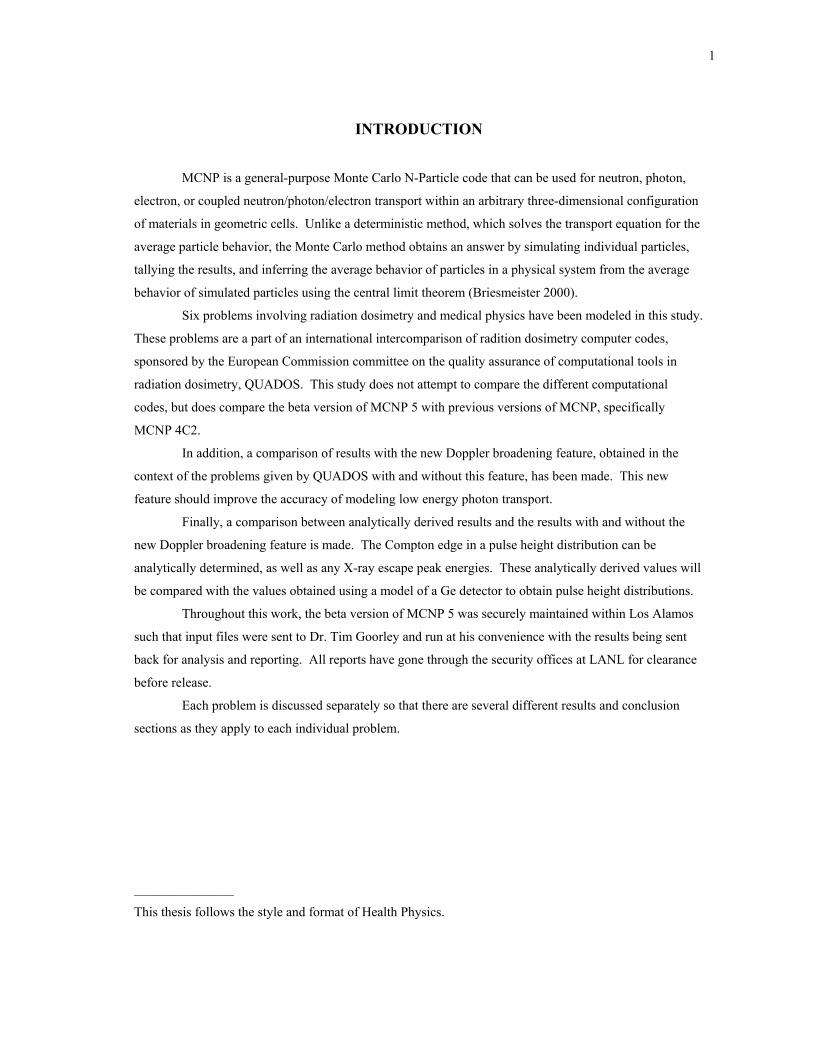
MCNP is a general-purpose Monte Carlo N-Particle code that can be used for neutron, photon,
electron, or coupled neutron/photon/electron transport within an arbitrary three-dimensional configuration
of materials in geometric cells. Unlike a deterministic method, which solves the transport equation for the
average particle behavior, the Monte Carlo method obtains an answer by simulating individual particles,
tallying the results, and inferring the average behavior of particles in a physical system from the average
behavior of simulated particles using the central limit theorem (Briesmeister 2000).
Six problems involving radiation dosimetry and medical physics have been modeled in this study.
These problems are a part of an international intercomparison of radition dosimetry computer codes,
sponsored by the European Commission committee on the quality assurance of computational tools in
radiation dosimetry, QUADOS. This study does not attempt to compare the different computational
codes, but does compare the beta version of MCNP 5 with previous versions of MCNP, specifically
MCNP 4C2.
In addition, a comparison of results with the new Doppler broadening feature, obtained in the
context of the problems given by QUADOS with and without this feature, has been made. This new
feature should improve the accuracy of modeling low energy photon transport.
Finally, a comparison between analytically derived results and the results with and without the
new Doppler broadening feature is made. The Compton edge in a pulse height distribution can be
analytically determined, as well as any X-ray escape peak energies. These analytically derived values will
be compared with the values obtained using a model of a Ge detector to obtain pulse height distributions.
Throughout this work, the beta version of MCNP 5 was securely maintained within Los Alamos
such that input files were sent to Dr. Tim Goorley and run at his convenience with the results being sent
back for analysis and reporting. All reports have gone through the security offices at LANL for clearance
before release.
Each problem is discussed separately so that there are several different results and conclusion
sections as they apply to each individual problem.
_______________
This thesis follows the style and format of Health Physics.
2
BACKGROUND
QUADOS
The international intercomparison consists of eight benchmark problems. The results were
originally due 15 October 2002, but were extended to 20 January 2003, for participants who worked on
multiple problems. These benchmark problems are intended to:
provide a snapshot of the methods and codes currently in use,
furnish information on the methods used to assess the reliability of computational results,
disseminate “good practice” throughout the radiation dosimetry community,
provide the users of computational codes with an opportunity to quality assure their own
procedures,
inform the radiation safety and medical physics communities about the benefits to be
obtained from sensitivity and uncertainty analysis, and
inform the above communities about the more sophisticated computational dosimetry
approaches that may be available to them (Siebert 2003).
The eight problems suggested in the QUADOS study are:
1. 192Ir brachytherapy source problem
2. Endovascular radiotherapy problem
3. Dose distribution of a proton beam in a water phantom
4. Neutron and/or photon response of a TLD-albedo personal dosimeter on an ISO slab
phantom
5. Air kerma backscatter profiles for two ISO photon expanded and aligned fields
impinging on the ISO water phantom
6. Calibration of neutron detectors in a bunker
7. Peak efficiencies and pulse height distributions of a photon germanium spectrometer in
the energy range below 1 MeV
8. Constancy check source.
Seven of these problems were attempted. Problems three and eight could not be accomplished
because the first involves proton dose to a spherical water phantom, which cannot be modeled in MCNP
version 5 because it lacks the capability to transport either protons or alpha particles. There was also not
enough information provided in problem eight to complete it.
Results of the intercomparison will hopefully point out which methods and codes are more
reliable, accurate, and perhaps easier to use in the context of these problems. It may also point out some
of the weaknesses of various codes. For example, MCNP is not very good at transporting low energy
photons. The germanium spectrometer problem has shown that a 15 keV photon incident upon the
3
detector will produce only the most significant of interactions. Other interactions result in either no tally
within the given bin or a result with significant error. While the new Doppler broadening feature attempts
to address this lack of accuracy for low energy photons, additional computational methods are needed, like
perhaps the S(α,β) cross sections employed with the physics of low energy neutrons. Other codes may
already take this into account and may produce more accurate results for the same problem. By knowing
which programs will work best in which areas we will be able to further increase the accuracy of our
modeling.
MCNP vs. Deterministic Method
Deterministic transport methods solve a transport equation for the average particle behavior
throughout the phase space of the problem. For example, the discrete ordinates method will divide phase
space into many small boxes for particles to travel within. As the volumes of the boxes are decreased,
these particles will take a differential amount of time to move a differential distance in space. In the limit
this approaches the integro-differential transport equation, which has derivatives in space and time. The
Monte Carlo method obtains an answer by simulating individual particles and tallying certain aspects of
their behavior such as the number of 6Li neutron capture reactions, 6Li(n,t)4He. The average behavior of
particles in a physical system is then inferred from the average behavior of the simulated particles using
the central limit theorem. The tallied aspects of the simulated particles’ behavior are then the obtained
answer. This method transports particles in space and time so it is sometimes said this solves the integral
transport equation, which does not have time or space derivatives (Briesmeister 2000).
Doppler Broadening
When incoherent scattering of an incident photon occurs, producing a Compton electron and a
scattered photon, the effect of the electron binding energy on the energy of the scattered photon has been
ignored in previous MCNP versions. The electron binding energy will also affect the angle of the
scattered photon, but this has already been taken into account by modifying the Klein-Nishina differential
cross section with a form factor. The effect of binding energy on the energy of the scattered photon is to
broaden the energy spectrum due to the precollision momentum of the electron. A new feature takes this
into account by using the Hartree-Fock Compton profile to sample the projected momentum and to
directly calculate the final energy of the scattered photon (Sood 2002).
4
PROBLEM ONE: 192Ir BRACHYTHERAPY SOURCE
Description of Problem
The first two problems are high-dose brachytherapy devices. Brachytherapy is a medical
procedure in which a radioactive source is placed within a body cavity or tumor (interstitial), or in close
proximity to a tumor (intercavitary) (Bast et al. 2000). These two problems specifically focus on
endovascular or vascular brachytherapy use following balloon angioplasty to prevent restenosis caused by
intimal hyperplasia, or the re-closing of the plaque, which would again block the artery.
The different brachytherapy devices are designed to provide a high dose, typically 12 Gy, to the
plaque and surface of the artery with very little dose to surrounding tissue, making it a more attractive
choice than for example, an external beam. This is possible due to the physical configuration of the
catheters. An algorithm has been developed to calculate near-field dose with these devices, but has been
reported to contain errors in the radial dose and anisotropy functions. Problem one repeats work that has
been previously published pointing out these errors with MCNP 4A (Wong et al. 1999).
This brachytherapy device uses a gamma source, 192Ir, to deliver a high dose-rate in the near-field
(defined to be < 5 cm by the author of the problem, Dr. Robert Price) to surrounding water. The dose is
determined for both radial and anisotropic distributions using a beta version of MCNP 5. This version did
not include the Doppler broadening feature. The anisotropic distribution is in ten-degree increments from
0o to 180o with 0o defined to be the axis through the center of the device along the woven steel cable. The
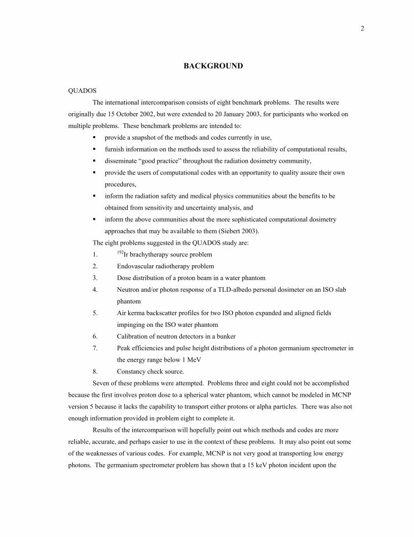
anistropic dose distribution was determined by cutting the surrounding sphere into wedges with 10o width
and tallying within these cells as shown in Fig. 1, below.
Fig. 1. Side view of anisotropic brachytherapy model. The angular tally cells are wedges of a sphere
cut at 10o increments. Radius of 192Ir core is 0.065 cm.
5
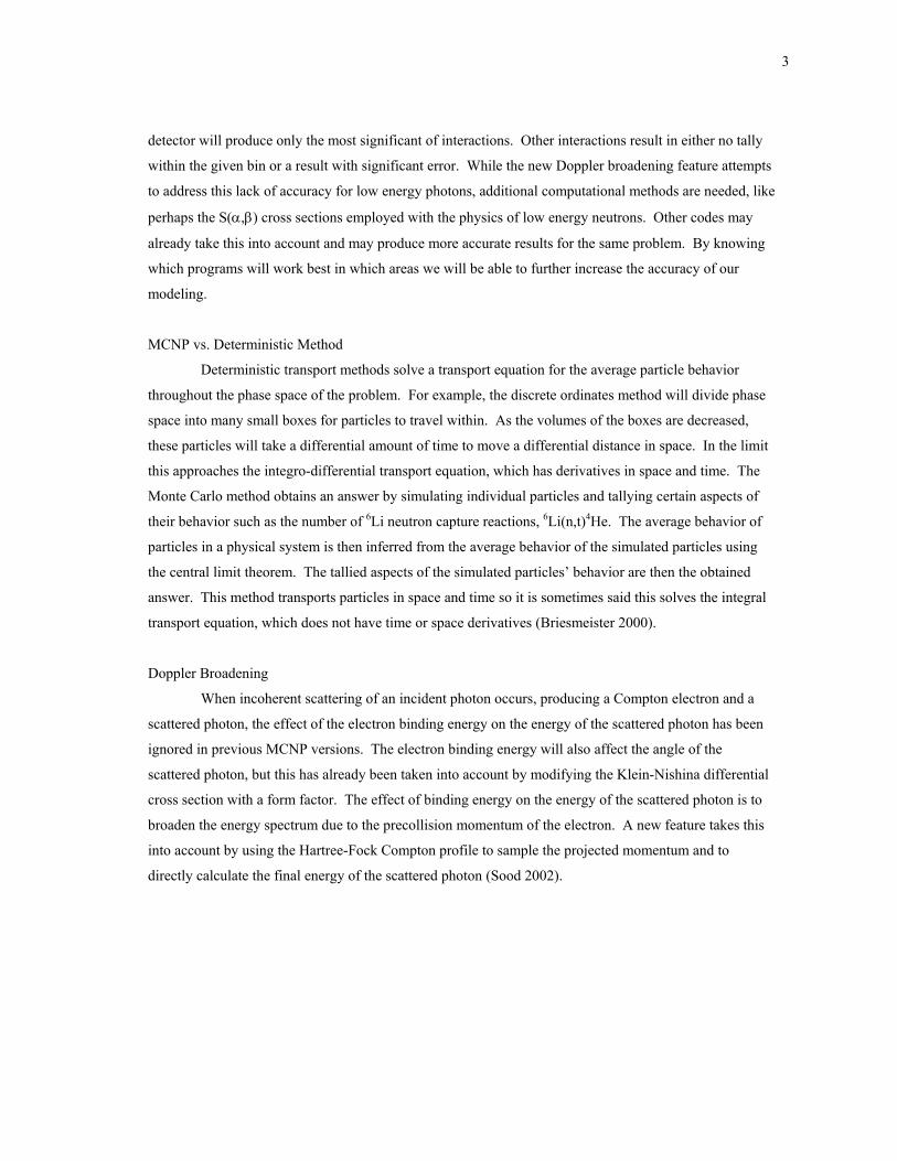
The radial distribution was determined with concentric cylinders about the source cylinder as
shown in Fig. 2, below. APPENDIX A contains example input files for all of the problems.
Fig. 2. Side view of radial brachytherapy model. The radial tally cells are cylinders with increasing
radii of 0.5 cm.
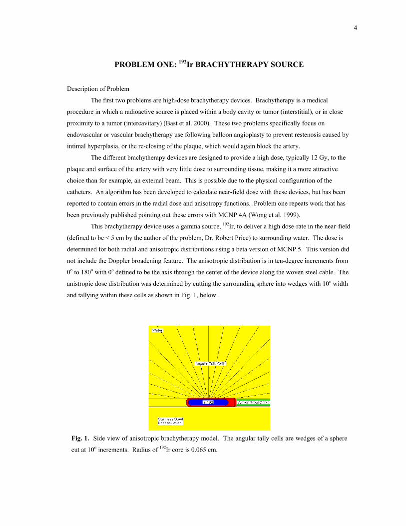
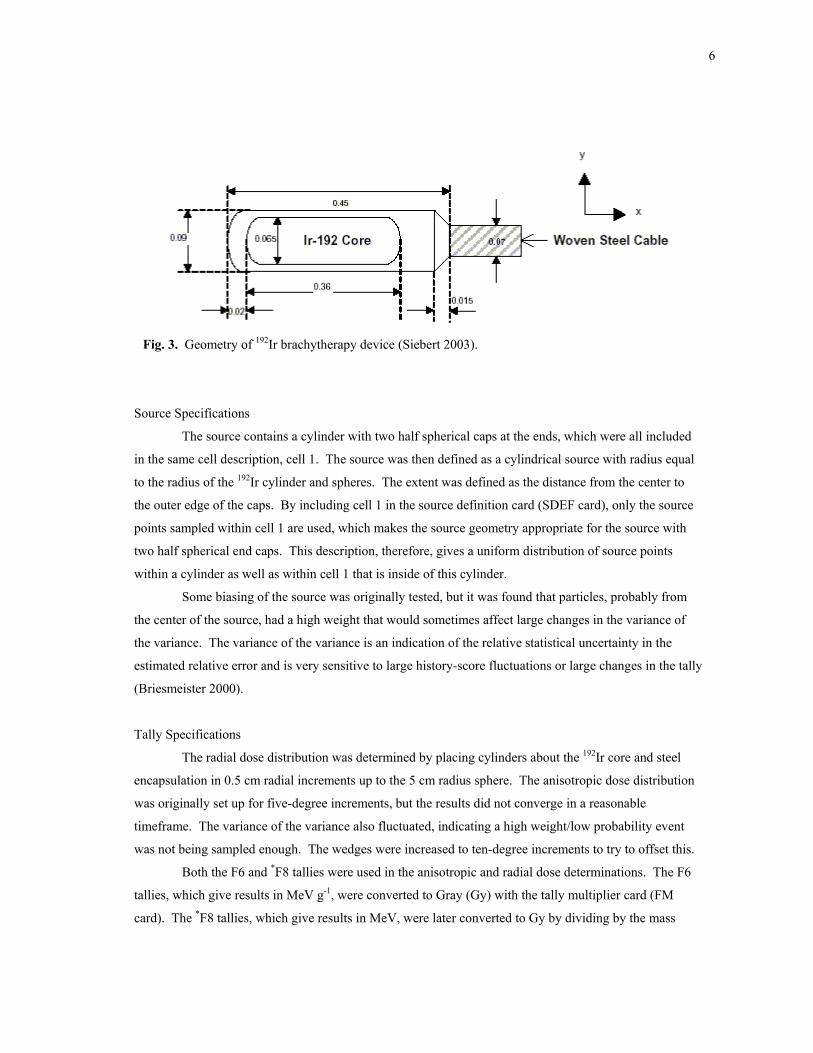
Geometry Specifications
The 192Ir brachytherapy device, which is shown in Fig. 3 on the next page, is an 192Ir core cylinder
with radius 0.0325 cm geometrically centered at the origin. It is capped at both ends by half spheres with
the same radii to give a total length of 0.36 cm. This 192Ir core is encased in a stainless steel cylinder,
radius 0.045 cm, with a half sphere cap, radius 0.061 cm, at one end and a cone that connects to the woven
steel cable to give a maximum length of 0.45 cm to the steel encapsulation. The material of the capsule
and cable is the same steel but with different densities. It has been assumed that the demarcation between
the two different densities is at the smaller end of the cone. A 5 cm radius sphere filled with water
surrounds the device, which also serves as the boundary of the problem (Siebert 2003).
6
Fig. 3. Geometry of 192Ir brachytherapy device (Siebert 2003).
Source Specifications
The source contains a cylinder with two half spherical caps at the ends, which were all included
in the same cell description, cell 1. The source was then defined as a cylindrical source with radius equal
to the radius of the 192Ir cylinder and spheres. The extent was defined as the distance from the center to
the outer edge of the caps. By including cell 1 in the source definition card (SDEF card), only the source
points sampled within cell 1 are used, which makes the source geometry appropriate for the source with
two half spherical end caps. This description, therefore, gives a uniform distribution of source points
within a cylinder as well as within cell 1 that is inside of this cylinder.
Some biasing of the source was originally tested, but it was found that particles, probably from
the center of the source, had a high weight that would sometimes affect large changes in the variance of
the variance. The variance of the variance is an indication of the relative statistical uncertainty in the
estimated relative error and is very sensitive to large history-score fluctuations or large changes in the tally
(Briesmeister 2000).
Tally Specifications
The radial dose distribution was determined by placing cylinders about the 192Ir core and steel
encapsulation in 0.5 cm radial increments up to the 5 cm radius sphere. The anisotropic dose distribution
was originally set up for five-degree increments, but the results did not converge in a reasonable
timeframe. The variance of the variance also fluctuated, indicating a high weight/low probability event
was not being sampled enough. The wedges were increased to ten-degree increments to try to offset this.
Both the F6 and *F8 tallies were used in the anisotropic and radial dose determinations. The F6
tallies, which give results in MeV g-1, were converted to Gray (Gy) with the tally multiplier card (FM
card). The *F8 tallies, which give results in MeV, were later converted to Gy by dividing by the mass
7
within the cell and multiplying by 6.02E-10 to convert the units from MeV g-1 to J kg-1 (Gy). The mass
within the cell was determined by multiplying the density of material in the cell by the volume of the cell.
Results
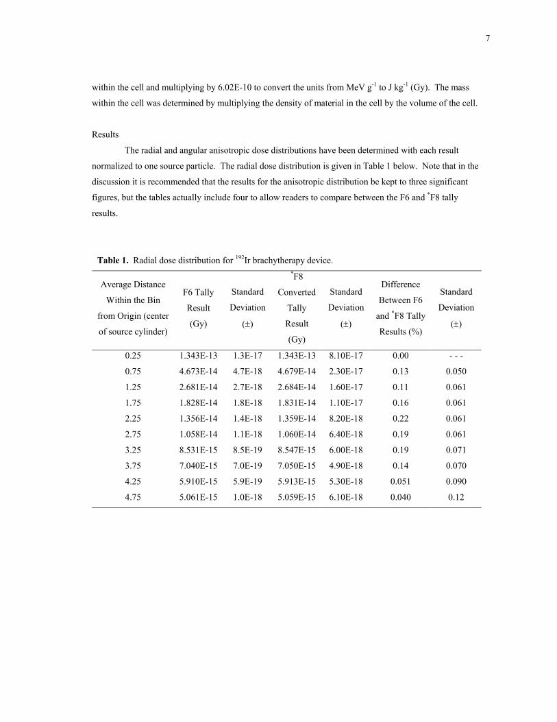
The radial and angular anisotropic dose distributions have been determined with each result
normalized to one source particle. The radial dose distribution is given in Table 1 below. Note that in the
discussion it is recommended that the results for the anisotropic distribution be kept to three significant
figures, but the tables actually include four to allow readers to compare between the F6 and *F8 tally
results.
Table 1. Radial dose distribution for 192Ir brachytherapy device.
Average Distance
Within the Bin
from Origin (center
of source cylinder)
F6 Tally
Result
(Gy)
Standard
Deviation
(±)
*F8
Converted
Tally
Result
(Gy)
Standard
Deviation
(±)
Difference
Between F6
and *F8 Tally
Results (%)
Standard
Deviation
(±)
0.25 1.343E-13 1.3E-17 1.343E-13 8.10E-17 0.00 - - -
0.75 4.673E-14 4.7E-18 4.679E-14 2.30E-17 0.13 0.050
1.25 2.681E-14 2.7E-18 2.684E-14 1.60E-17 0.11 0.061
1.75 1.828E-14 1.8E-18 1.831E-14 1.10E-17 0.16 0.061
2.25 1.356E-14 1.4E-18 1.359E-14 8.20E-18 0.22 0.061
2.75 1.058E-14 1.1E-18 1.060E-14 6.40E-18 0.19 0.061
3.25 8.531E-15 8.5E-19 8.547E-15 6.00E-18 0.19 0.071
3.75 7.040E-15 7.0E-19 7.050E-15 4.90E-18 0.14 0.070
4.25 5.910E-15 5.9E-19 5.913E-15 5.30E-18 0.051 0.090
4.75 5.061E-15 1.0E-18 5.059E-15 6.10E-18 0.040 0.12
8
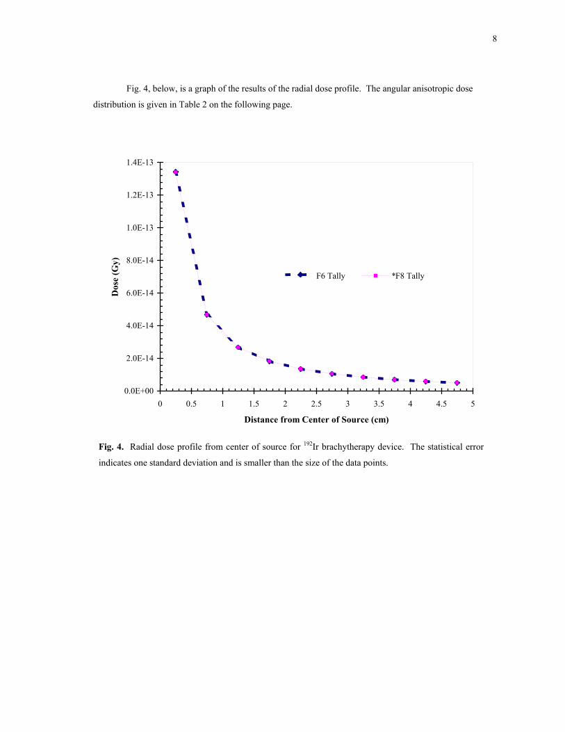
Fig. 4, below, is a graph of the results of the radial dose profile. The angular anisotropic dose
distribution is given in Table 2 on the following page.
0.0E+00
2.0E-14
4.0E-14
6.0E-14
8.0E-14
1.0E-13
1.2E-13
1.4E-13
0 0.5 1 1.5 2 2.5 3 3.5 4 4.5 5
Distance from Center of Source (cm)
Dos
e (G
y)
F6 Tally *F8 Tally
Fig. 4. Radial dose profile from center of source for 192Ir brachytherapy device. The statistical error
indicates one standard deviation and is smaller than the size of the data points.
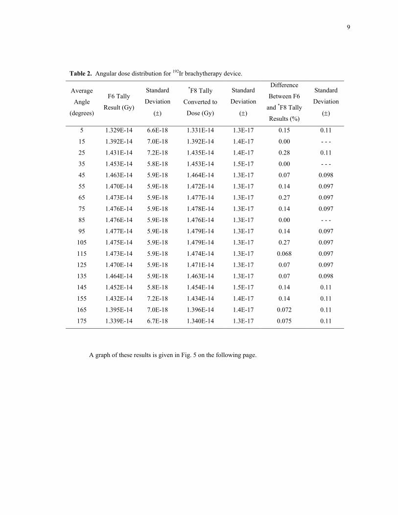
9
Table 2. Angular dose distribution for 192Ir brachytherapy device.
Average
Angle
(degrees)
F6 Tally
Result (Gy)
Standard
Deviation
(±)
*F8 Tally
Converted to
Dose (Gy)
Standard
Deviation
(±)
Difference
Between F6
and *F8 Tally
Results (%)
Standard
Deviation
(±)
5 1.329E-14 6.6E-18 1.331E-14 1.3E-17 0.15 0.11
15 1.392E-14 7.0E-18 1.392E-14 1.4E-17 0.00 - - -
25 1.431E-14 7.2E-18 1.435E-14 1.4E-17 0.28 0.11
35 1.453E-14 5.8E-18 1.453E-14 1.5E-17 0.00 - - -
45 1.463E-14 5.9E-18 1.464E-14 1.3E-17 0.07 0.098
55 1.470E-14 5.9E-18 1.472E-14 1.3E-17 0.14 0.097
65 1.473E-14 5.9E-18 1.477E-14 1.3E-17 0.27 0.097
75 1.476E-14 5.9E-18 1.478E-14 1.3E-17 0.14 0.097
85 1.476E-14 5.9E-18 1.476E-14 1.3E-17 0.00 - - -
95 1.477E-14 5.9E-18 1.479E-14 1.3E-17 0.14 0.097
105 1.475E-14 5.9E-18 1.479E-14 1.3E-17 0.27 0.097
115 1.473E-14 5.9E-18 1.474E-14 1.3E-17 0.068 0.097
125 1.470E-14 5.9E-18 1.471E-14 1.3E-17 0.07 0.097
135 1.464E-14 5.9E-18 1.463E-14 1.3E-17 0.07 0.098
145 1.452E-14 5.8E-18 1.454E-14 1.5E-17 0.14 0.11
155 1.432E-14 7.2E-18 1.434E-14 1.4E-17 0.14 0.11
165 1.395E-14 7.0E-18 1.396E-14 1.4E-17 0.072 0.11
175 1.339E-14 6.7E-18 1.340E-14 1.3E-17 0.075 0.11
A graph of these results is given in Fig. 5 on the following page.
10
1.32E-14
1.34E-14
1.36E-14
1.38E-14
1.40E-14
1.42E-14
1.44E-14
1.46E-14
1.48E-14
1.50E-14
0 20 40 60 80 100 120 140 160 180
Polar Angle (degrees) Relative to Cable Axis
Dos
e (G
y)
Results From F6 Tally
Results From *F8 Tally
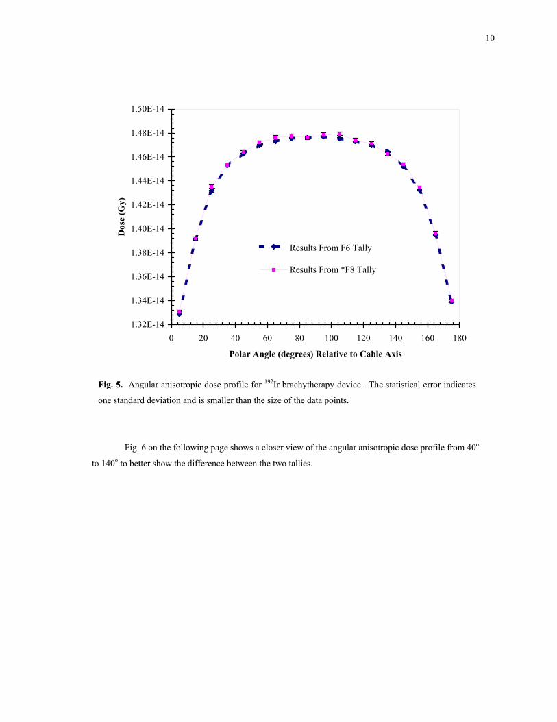
Fig. 5. Angular anisotropic dose profile for 192Ir brachytherapy device. The statistical error indicates
one standard deviation and is smaller than the size of the data points.
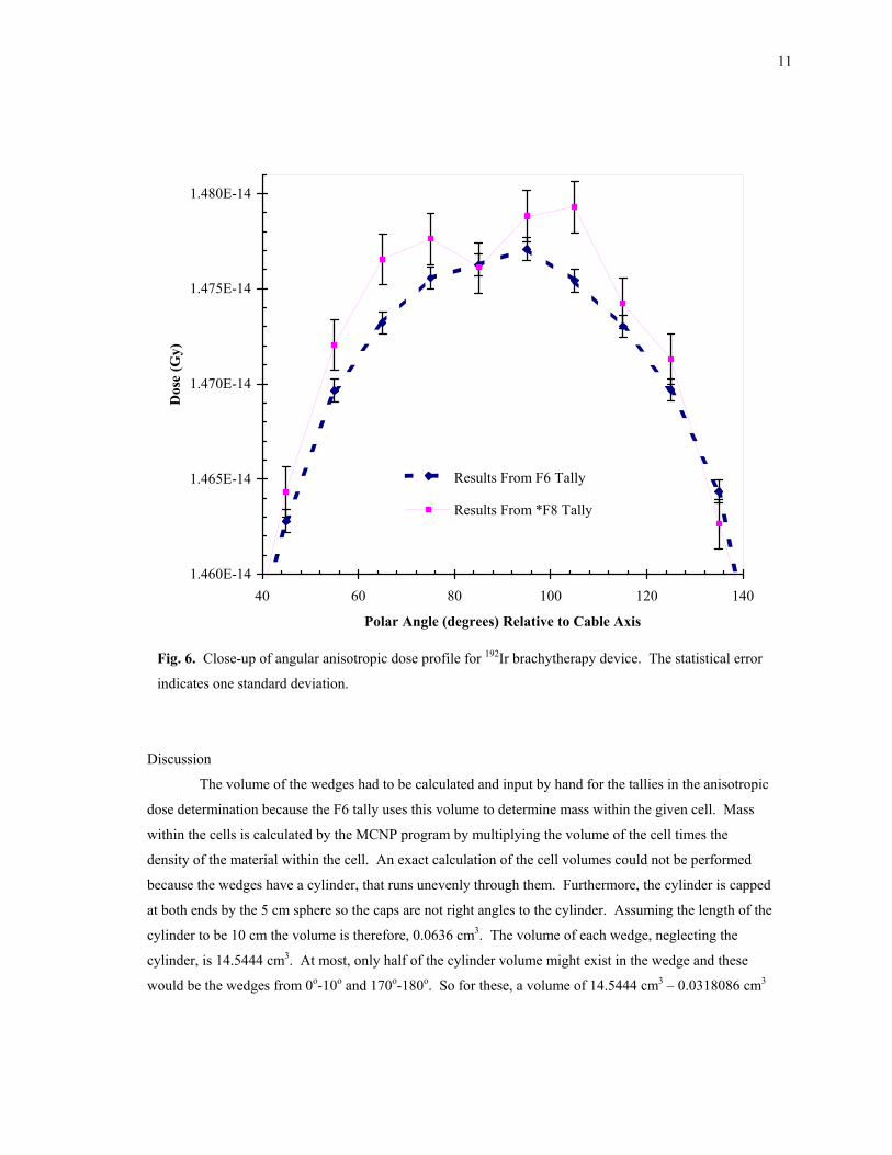
Fig. 6 on the following page shows a closer view of the angular anisotropic dose profile from 40o
to 140o to better show the difference between the two tallies.
11
1.460E-14
1.465E-14
1.470E-14
1.475E-14
1.480E-14
40 60 80 100 120 140
Polar Angle (degrees) Relative to Cable Axis
Dos
e (G
y)
Results From F6 Tally
Results From *F8 Tally
Fig. 6. Close-up of angular anisotropic dose profile for 192Ir brachytherapy device. The statistical error
indicates one standard deviation.
Discussion
The volume of the wedges had to be calculated and input by hand for the tallies in the anisotropic
dose determination because the F6 tally uses this volume to determine mass within the given cell. Mass
within the cells is calculated by the MCNP program by multiplying the volume of the cell times the
density of the material within the cell. An exact calculation of the cell volumes could not be performed
because the wedges have a cylinder, that runs unevenly through them. Furthermore, the cylinder is capped
at both ends by the 5 cm sphere so the caps are not right angles to the cylinder. Assuming the length of the
cylinder to be 10 cm the volume is therefore, 0.0636 cm3. The volume of each wedge, neglecting the
cylinder, is 14.5444 cm3. At most, only half of the cylinder volume might exist in the wedge and these
would be the wedges from 0o-10o and 170o-180o. So for these, a volume of 14.5444 cm3 – 0.0318086 cm3
12
= 14.5126 cm3 was used while for the rest the 14.5444 cm3 volume was used. This introduces some error,
but if the results are limited to three significant figures it should not make any difference.
The graph in Fig. 3 uses the same volumes in the calculations of the F6 and *F8 tallies allowing
the two to be compared. In this problem, the two tallies compared well with differences in tally results
after the third significant figure. The percent-difference in the radial dose distribution ranged from 0.0 –
0.22%, while the range for the angular anisotropic distribution went from 0.0 – 0.28%. However, both had
significant error associated with the percent-difference as shown in Tables 1 and 2. It is interesting to note
that the standard deviation for the F6 tally results were often outside the standard deviation for the *F8
tally results. The precision of the F6 tally was found to be smaller by about a half an order of magnitude
than the *F8 tally.
13
PROBLEM TWO: 32P BRACHYTHERAPY SOURCE
Description of Problem
The second problem uses a 32P source to provide beta dose to the arterial wall. The following
was determined:
• the dose rate was measured at a depth of 1 mm into the artery wall from the
inside surface along the source longitudinal axis;
• the radial dose rate profile; and
• the dose rate at 1 mm depth inside the artery wall at the center of the
source longitudinal axis.
To obtain a good profile of the dose rate along the source longitudinal axis, the blood and artery
wall were divided into rings so the weight window generator could be applied. Originally, the source was
biased so that more particles were sampled at the ends of the source cylinder. This was found to give
erroneous results near the center of the source cylinder because of a low sampling frequency. This was
corrected by rerunning without any source biasing.
Geometry Specifications
For this problem the balloon apparatus, which would center the catheter, was not modeled, as
directed by the author of the problem, Dr. Robert Price. The 32P source is a cylinder geometrically
centered on the origin along the y-axis with radius 0.012 cm and length 2.7 cm. It is surrounded by a NiTi
tube of inner radius 0.0154 cm and outer radius 0.023 cm (wall thickness of 0.0076 cm). A symmetric air
space exists between the 32P source cylinder and the NiTi cylinder wall. At the closed end of the 32P
source is a tungsten marker of length 0.1 cm followed by a NiTi plug also of length 0.1 cm. Both the
marker and plug are the same radius as the 32P source. Beyond the NiTi plug is a NiTi hemispherical
weld. The radius is assumed to be the same radius as the outside wall of the NiTi tube, 0.023 cm. At the
other end of the source cylinder is the NiTi guide wire. It has a radius equal to the inner radius of the NiTi
tube, 0.0154 cm. The wire contacts the 32P source with another half sphere that is assumed to be of the
same radius as the wire, 0.0154 cm. The wire and tube both continue to the end of the phantom. Outside
of the NiTi tube is the blood which ends at the inner wall of the artery, also a cylinder with radius 0.15 cm
and outer wall radius 0.35 cm. Beyond the artery wall is the water phantom that extends to a radius of 15
cm and length of 30 cm. Outside of the water phantom is defined as outside of the problem, or void
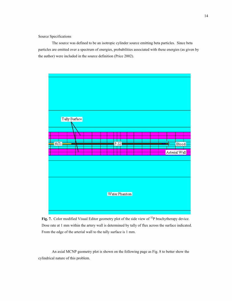
(Siebert 2003). A geometry plot, Fig. 7, using the Visual Editor of the side view is on the following page.
14
Source Specifications
The source was defined to be an isotropic cylinder source emitting beta particles. Since beta
particles are emitted over a spectrum of energies, probabilities associated with these energies (as given by
the author) were included in the source definition (Price 2002).
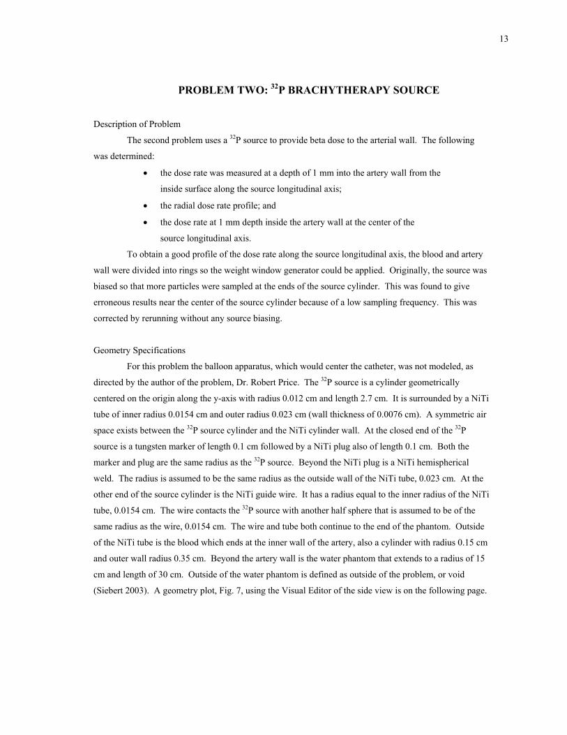
Fig. 7. Color modified Visual Editor geometry plot of the side view of 32P brachytherapy device.
Dose rate at 1 mm within the artery wall is determined by tally of flux across the surface indicated.
From the edge of the arterial wall to the tally surface is 1 mm.
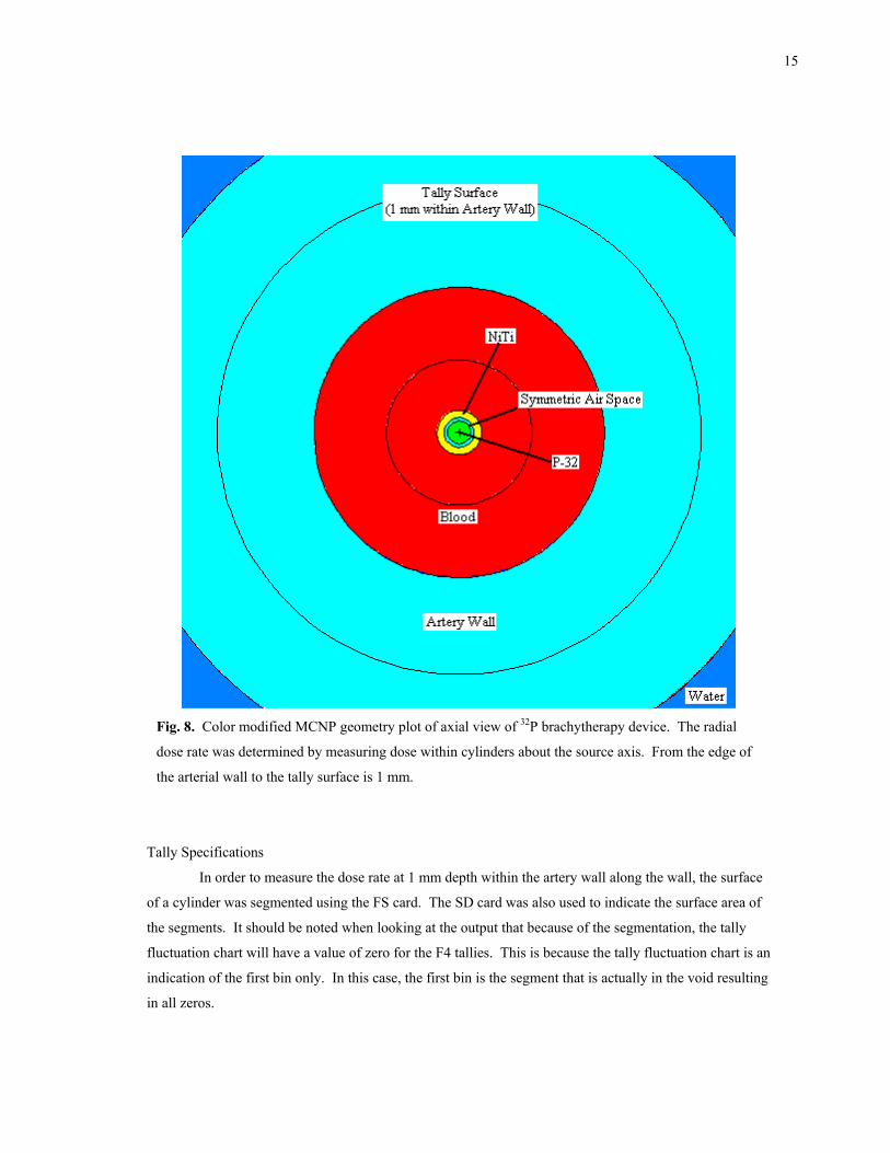
An axial MCNP geometry plot is shown on the following page as Fig. 8 to better show the
cylindrical nature of this problem.
15
Fig. 8. Color modified MCNP geometry plot of axial view of 32P brachytherapy device. The radial
dose rate was determined by measuring dose within cylinders about the source axis. From the edge of
the arterial wall to the tally surface is 1 mm.
Tally Specifications
In order to measure the dose rate at 1 mm depth within the artery wall along the wall, the surface
of a cylinder was segmented using the FS card. The SD card was also used to indicate the surface area of
the segments. It should be noted when looking at the output that because of the segmentation, the tally
fluctuation chart will have a value of zero for the F4 tallies. This is because the tally fluctuation chart is an
indication of the first bin only. In this case, the first bin is the segment that is actually in the void resulting
in all zeros.

16
DE and DF cards were also used to convert MeV cm-2 to Gy. Values used in the DE and DF
cards are the electron energy and mass collison stopping powers for adipose tissue (ICRP), respectively.
Adipose tissue was the closest material in atomic composition with available mass collision stopping
powers (Attix 1986).
Variance Reduction
To better sample the far ends of the cylinder of the artery wall, the cells were divided into rings.
The weight window generator was then used to optimize electron flux on surface 24, which is the cylinder
1 mm into the artery wall from the inside. To further assist in getting a good weight window, the densities
of all of the materials were lowered and the energy of the source electron changed to 10 MeV so that the
electrons would travel further. The material densities and particle energy were changed back after
generating the weight window mesh file.
Results
The input file was run twice. The first run included the biasing of the source with greater
frequency of source particles occurring at the ends of the cylinder. The radial dose distribution from the
center of the source cylinder was obtained from this result along with a better idea of the axial dose
profile. The second run was used to obtain the dose profile along the axis of the artery wall. Results for
the radial dose profile are given in Table 3, on the next page. The slope of the radial dose rate profile did
not meet the statistical criteria of >3 with a value of 2.55. The slope is one of the statistical checks
indicating whether enough particles have been simulated to satisfy the central limit theorem. Other
statistical checks did pass. Results for the second run are given in Table 4, on the following page, with a
graph of the results from both runs in Fig. 9. In all cases, the dose was normalized to a single particle, but
later multiplied by 7E09 to convert to a 7 GBq source.
17
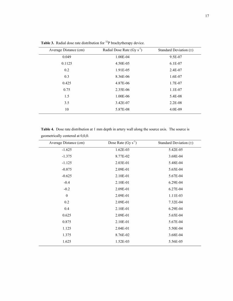
Table 3. Radial dose rate distribution for 32P brachytherapy device.
Average Distance (cm) Radial Dose Rate (Gy s-1) Standard Deviation (±)
0.049 1.00E-04 9.5E-07
0.1125 4.50E-05 6.1E-07
0.2 1.91E-05 2.4E-07
0.3 8.36E-06 1.6E-07
0.425 4.87E-06 1.7E-07
0.75 2.35E-06 1.1E-07
1.5 1.00E-06 5.4E-08
3.5 3.42E-07 2.2E-08
10 5.87E-08 4.0E-09
Table 4. Dose rate distribution at 1 mm depth in artery wall along the source axis. The source is
geometrically centered at 0,0,0.
Average Distance (cm) Dose Rate (Gy s-1) Standard Deviation (±)
-1.625 1.62E-03 5.42E-05
-1.375 8.77E-02 3.68E-04
-1.125 2.03E-01 5.48E-04
-0.875 2.09E-01 5.65E-04
-0.625 2.10E-01 5.67E-04
-0.4 2.10E-01 6.29E-04
-0.2 2.09E-01 6.27E-04
0 2.09E-01 1.11E-03
0.2 2.09E-01 7.32E-04
0.4 2.10E-01 6.29E-04
0.625 2.09E-01 5.65E-04
0.875 2.10E-01 5.67E-04
1.125 2.04E-01 5.50E-04
1.375 8.76E-02 3.68E-04
1.625 1.52E-03 5.56E-05
18
Dose rate at 1 mm within the artery wall along the midway point of the source cylinder is 2.09E-
01 ± 1.11E-03 Gy s-1. This was the average dose to the surface of a 0.2 cm width ring about the center of
the source cylinder 1 mm within the artery wall.
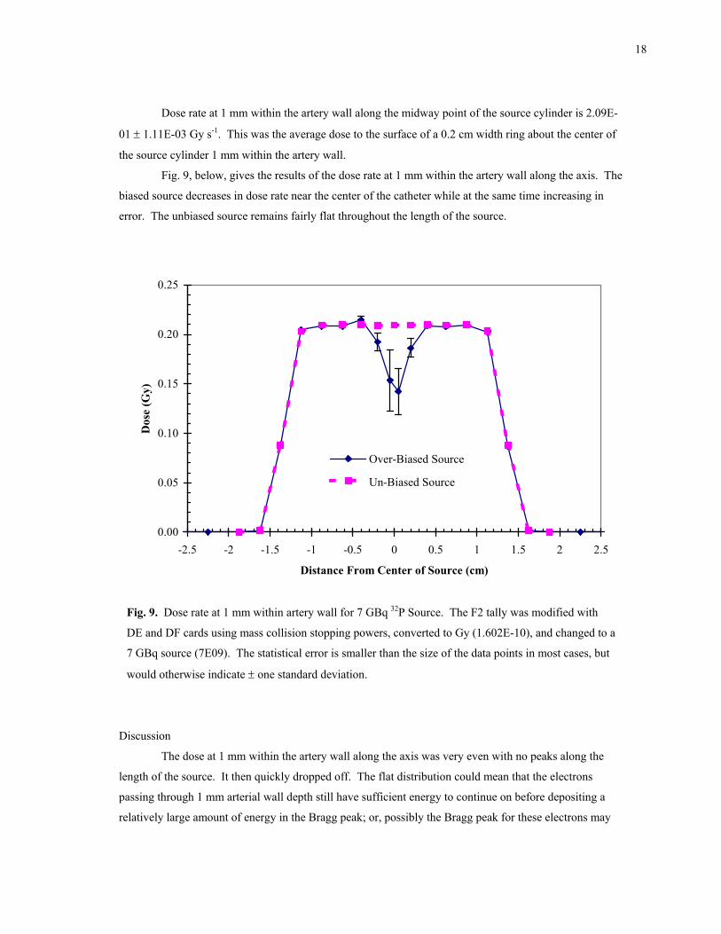
Fig. 9, below, gives the results of the dose rate at 1 mm within the artery wall along the axis. The
biased source decreases in dose rate near the center of the catheter while at the same time increasing in
error. The unbiased source remains fairly flat throughout the length of the source.
0.00
0.05
0.10
0.15
0.20
0.25
-2.5 -2 -1.5 -1 -0.5 0 0.5 1 1.5 2 2.5
Distance From Center of Source (cm)
Dos
e (G
y)
Over-Biased Source
Un-Biased Source
Fig. 9. Dose rate at 1 mm within artery wall for 7 GBq 32P Source. The F2 tally was modified with
DE and DF cards using mass collision stopping powers, converted to Gy (1.602E-10), and changed to a
7 GBq source (7E09). The statistical error is smaller than the size of the data points in most cases, but
would otherwise indicate ± one standard deviation.
Discussion
The dose at 1 mm within the artery wall along the axis was very even with no peaks along the
length of the source. It then quickly dropped off. The flat distribution could mean that the electrons
passing through 1 mm arterial wall depth still have sufficient energy to continue on before depositing a
relatively large amount of energy in the Bragg peak; or, possibly the Bragg peak for these electrons may

19
be insufficient to affect the distribution significantly. If the axial dose were studied further away from the
source this might start to change the even profile to include a positive peak at the center.
The biased source dropped at the center of the source but the increasing relative error indicated
erroneous results. In this case, the standard deviation of the biased source was outside of the standard
deviation of the unbiased results.
20
PROBLEM FOUR: NEUTRON AND PHOTON RESPONSE OF A TLD-
ALBEDO PERSONAL DOSIMETER ON AN ISO SLAB PHANTOM
Problem Description
Photon and neutron responses in a four-element TLD-albedo personal dosimeter located on the
center of the front face of an ISO water filled slab phantom were determined using a beta version of
MCNP 5. This version did not include the Doppler broadening feature. Photon response for photons of
energy 33 keV, 48 keV, 100 keV, 248 keV, 662 keV, and 1.25 MeV were determined as energy absorbed
in the TLD, which was assumed to be proportional to light output. Neutron response for neutrons with
energies of 0.0253 eV, 1 eV, 10 eV, 100 eV, 1 keV, 10 keV, 100 keV, 1 MeV, 10 MeV, and 20 MeV were
determined as the number of 6Li(n,t)4He capture reactions, which was again assumed to be proportional to
the light output.
Comparisons of photons at energies of 33 kev, 48 keV, 100 keV, 248 keV and 1.25 MeV between
versions 4C2 and 5beta3.23 were made with each run ending at 50 million histories. These comparisons
began at the same random number and tracked. In addition, the 33 kev photon source was also run in
versions 4C3 and 5beta4.9 to compare computer time, ctm, only.
Neutron results using the S(α,β) cross sections were compared with results obtained without
these cross sections. The S(α,β) cross sections replace the free gas treatment of the particle physics at low
neutron energies with some consideration of bond energies and their effect upon elastically scattered
neutrons. In this problem, the bond energies of oxygen and hydrogen in water were taken into account in
the water of the slab phantom.
TLDs are often used in personal dosimetry throughout the radiation industry. The elements offer
a small and light device for measuring dose and when used with certain shielding materials, can
approximate different types of doses such as surface dose and neutron dose. For example, this problem
contains both 6Li and 7Li chips which would normally be compared to determine neutron dose. LiF
elements also offer a close match in effective atomic number, which when compared to that of soft tissue,
give a strong correlation to dose equivalent and exposure over a wide range of photon energies (Knoll
2000).
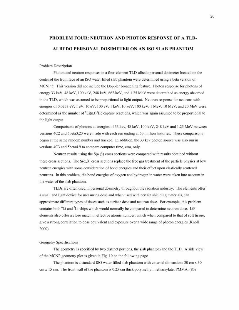
Geometry Specifications
The geometry is specified by two distinct portions, the slab phantom and the TLD. A side view
of the MCNP geometry plot is given in Fig. 10 on the following page.
The phantom is a standard ISO water filled slab phantom with external dimensions 30 cm x 30
cm x 15 cm. The front wall of the phantom is 0.25 cm thick polymethyl methacrylate, PMMA, (8%
21
hydrogen, 32% oxygen, and 60% carbon) while the remaining walls are all 1 cm thick PMMA. The
phantom is filled with water.
Fig. 10. Side view of MCNP geometry plot for problem 4.
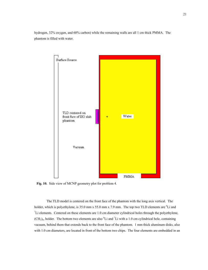
The TLD model is centered on the front face of the phantom with the long axis vertical. The
holder, which is polyethylene, is 35.0 mm x 55.0 mm x 7.9 mm. The top two TLD elements are 6Li and 7Li elements. Centered on these elements are 1.0 cm diameter cylindrical holes through the polyethylene,
(CH2)n, holder. The bottom two elements are also 6Li and 7Li with a 1.0 cm cylindrical hole, containing
vacuum, behind them that extends back to the front face of the phantom. 1 mm thick aluminum disks, also
with 1.0 cm diameters, are located in front of the bottom two chips. The four elements are embedded in an
22
aluminum plate that is 25.0 mm x 45.0 mm x 0.9 mm. The elements are each 3.2 mm x 3.2 mm x 0.9 mm
(Siebert 2003).
A front view of the TLD and depth view from the front surface are given to show shielding in
Fig. 11, below.
Front face of TLD 0.49 cm into TLD from front face
0.5 cm into the TLD from front face 0.59 cm into the TLD from front face
Fig. 11. MCNP geometry plot of front view of TLD followed by planar views within the TLD.
Source Specifications
The source is a surface source with the same dimension as the front face of the phantom, which
emits particles normal to the front face of the slab phantom and TLD. To better sample the photons and
23
neutrons about the TLD, the source was biased so that more particles started out directed towards the
TLD.
Photons of energies 33 keV, 48 keV, 100 keV, 248 keV, 662 keV, and 1.25 MeV were
individually examined and neutrons of energies 0.0253 eV, 1 eV, 10 eV, 100 eV, 1 keV, 100 keV, 1 MeV,
10 MeV, and 20 MeV were also individually examined.
Tally Specifications
F6 tallies for the cells corresponding to the TLD elements were used to determine photon energy
deposition while neutron response was measured as the number of 6Li(n,t)4He capture reactions. To count
the number of capture reactions the tally multiplier card, FM, was used in conjunction with the F4 tally to
specify which reaction to count. The result was then multiplied by the volume within the cell and a factor
to convert the density from atoms cc-1 to atoms (barns-cm)-1. The FM card requires an input of density
which was not in the correct units for all of the neutron results.
Variance Reduction
Since the TLD badge was small compared to the size of the slab phantom, very few particles
made it to the smaller LiF elements. Changing the importances of the cells was found to be insufficient to
increase the number of particles passing through the elements. A mesh was therefore created and used to
generate weight windows. This greatly improved the method with photon results usually converging
within 50 million source particles. The neutrons, however, often took up to 300 million source particles to
converge.
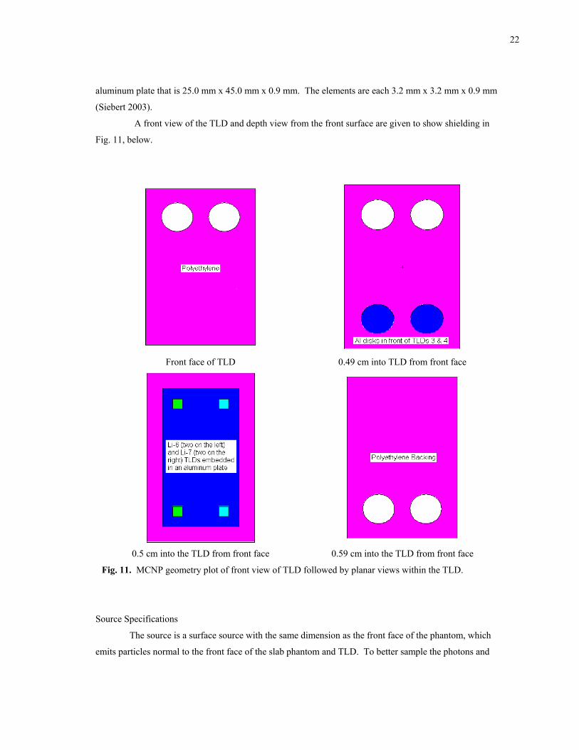
Results
Photon response was measured by determination of the amount of energy absorbed using the F6
tally. The results were multiplied by the mass within the cell to provide an answer in MeV. The results
for each of the photon energies are given in Table 5 on the following page. Each result is normalized to
one source particle.
24
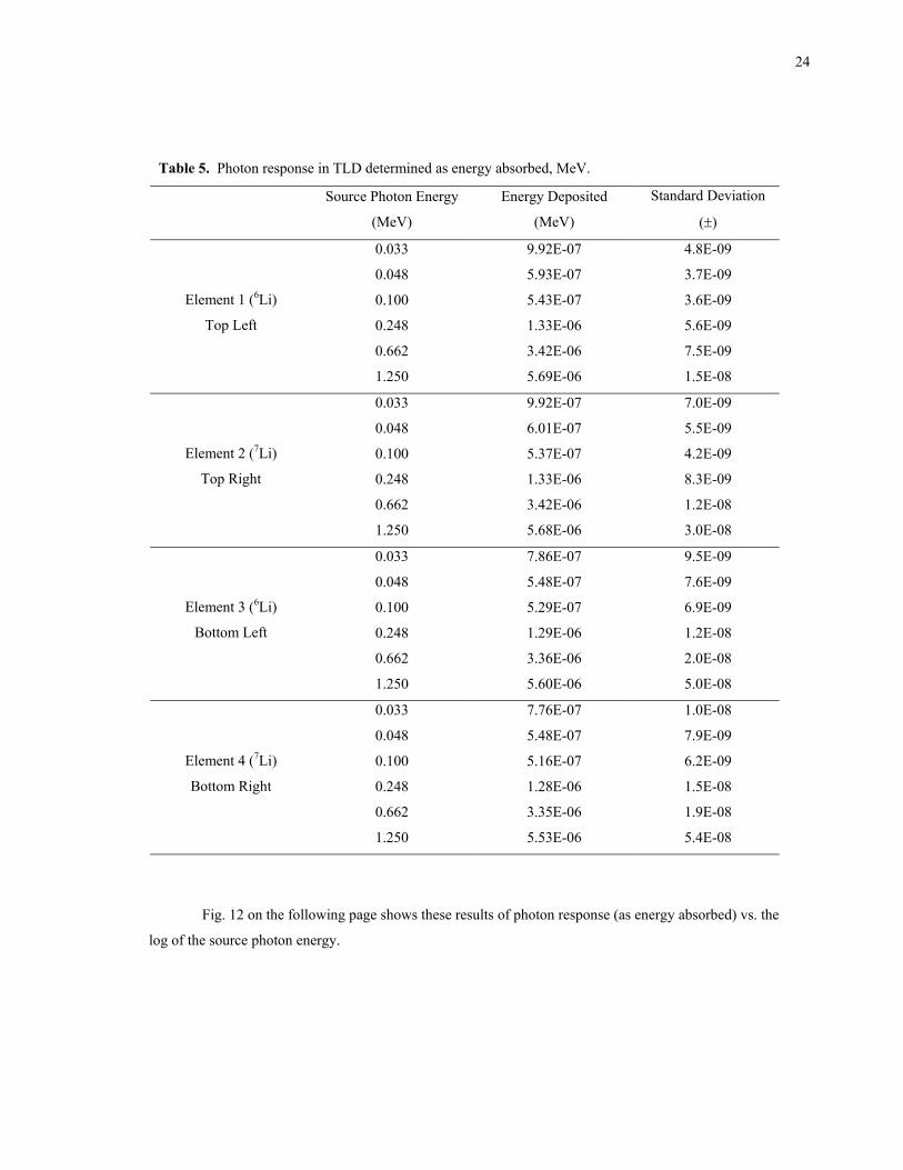
Table 5. Photon response in TLD determined as energy absorbed, MeV.
Source Photon Energy
(MeV)
Energy Deposited
(MeV)
Standard Deviation
(±)
0.033 9.92E-07 4.8E-09
0.048 5.93E-07 3.7E-09
0.100 5.43E-07 3.6E-09
0.248 1.33E-06 5.6E-09
0.662 3.42E-06 7.5E-09
Element 1 (6Li)
Top Left
1.250 5.69E-06 1.5E-08
0.033 9.92E-07 7.0E-09
0.048 6.01E-07 5.5E-09
0.100 5.37E-07 4.2E-09
0.248 1.33E-06 8.3E-09
0.662 3.42E-06 1.2E-08
Element 2 (7Li)
Top Right
1.250 5.68E-06 3.0E-08
0.033 7.86E-07 9.5E-09
0.048 5.48E-07 7.6E-09
0.100 5.29E-07 6.9E-09
0.248 1.29E-06 1.2E-08
0.662 3.36E-06 2.0E-08
Element 3 (6Li)
Bottom Left
1.250 5.60E-06 5.0E-08
0.033 7.76E-07 1.0E-08
0.048 5.48E-07 7.9E-09
0.100 5.16E-07 6.2E-09
0.248 1.28E-06 1.5E-08
0.662 3.35E-06 1.9E-08
Element 4 (7Li)
Bottom Right
1.250 5.53E-06 5.4E-08
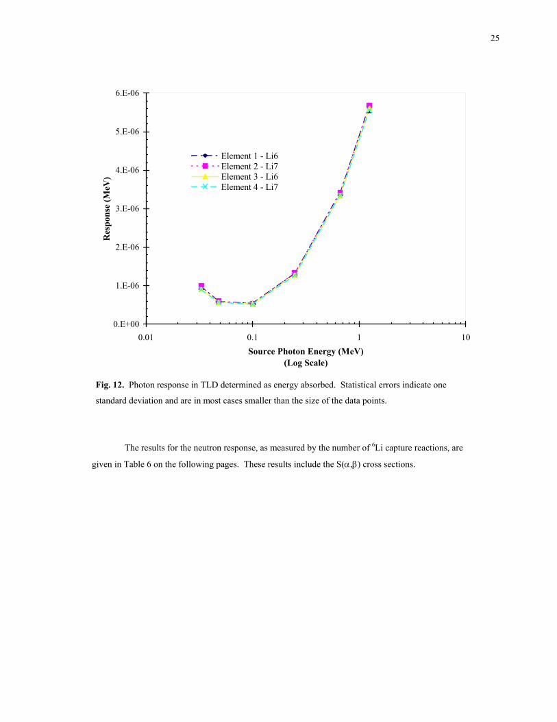
Fig. 12 on the following page shows these results of photon response (as energy absorbed) vs. the
log of the source photon energy.
25
0.E+00
1.E-06
2.E-06
3.E-06
4.E-06
5.E-06
6.E-06
0.01 0.1 1 10Source Photon Energy (MeV)
(Log Scale)
Res
pons
e (M
eV)
Element 1 - Li6Element 2 - Li7Element 3 - Li6Element 4 - Li7
Fig. 12. Photon response in TLD determined as energy absorbed. Statistical errors indicate one
standard deviation and are in most cases smaller than the size of the data points.
The results for the neutron response, as measured by the number of 6Li capture reactions, are
given in Table 6 on the following pages. These results include the S(α,β) cross sections.
26
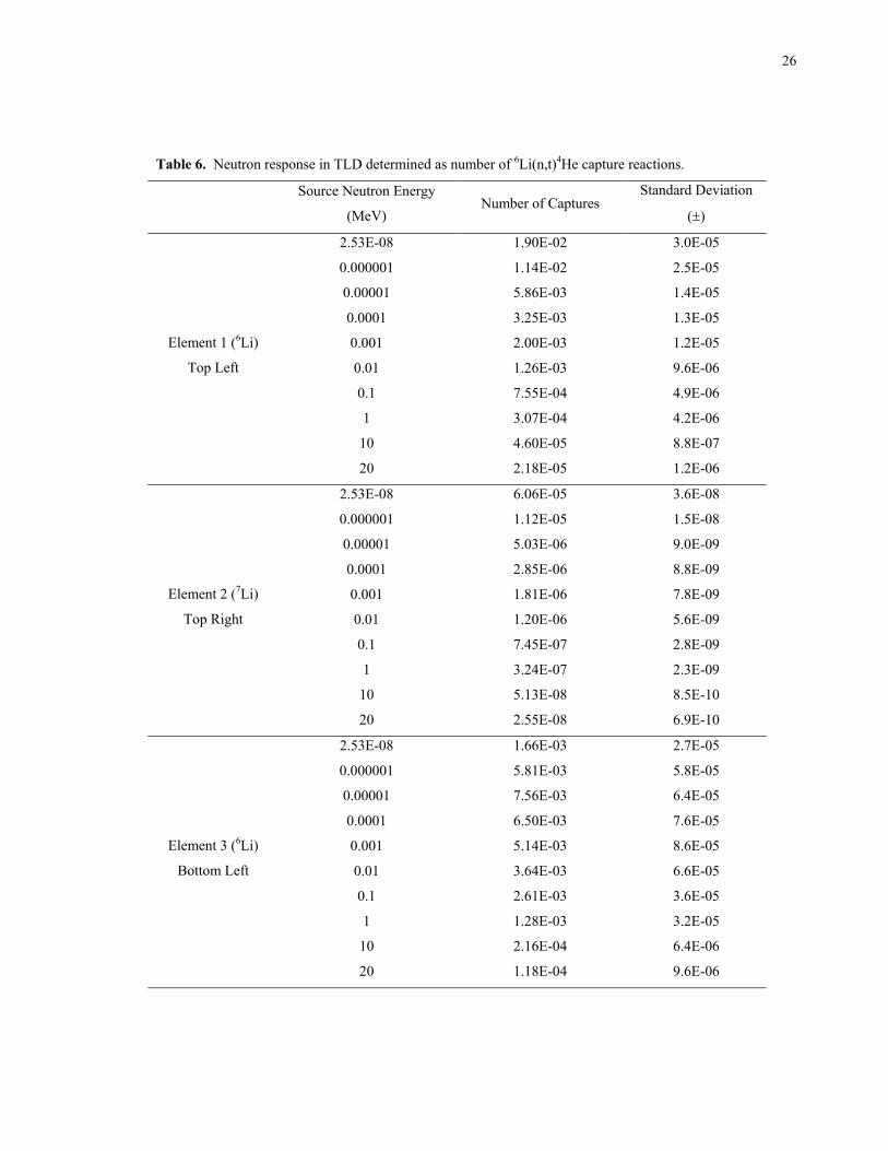
Table 6. Neutron response in TLD determined as number of 6Li(n,t)4He capture reactions.
Source Neutron Energy
(MeV) Number of Captures
Standard Deviation
(±)
2.53E-08 1.90E-02 3.0E-05
0.000001 1.14E-02 2.5E-05
0.00001 5.86E-03 1.4E-05
0.0001 3.25E-03 1.3E-05
0.001 2.00E-03 1.2E-05
0.01 1.26E-03 9.6E-06
0.1 7.55E-04 4.9E-06
1 3.07E-04 4.2E-06
10 4.60E-05 8.8E-07
Element 1 (6Li)
Top Left
20 2.18E-05 1.2E-06
2.53E-08 6.06E-05 3.6E-08
0.000001 1.12E-05 1.5E-08
0.00001 5.03E-06 9.0E-09
0.0001 2.85E-06 8.8E-09
0.001 1.81E-06 7.8E-09
0.01 1.20E-06 5.6E-09
0.1 7.45E-07 2.8E-09
1 3.24E-07 2.3E-09
10 5.13E-08 8.5E-10
Element 2 (7Li)
Top Right
20 2.55E-08 6.9E-10
2.53E-08 1.66E-03 2.7E-05
0.000001 5.81E-03 5.8E-05
0.00001 7.56E-03 6.4E-05
0.0001 6.50E-03 7.6E-05
0.001 5.14E-03 8.6E-05
0.01 3.64E-03 6.6E-05
0.1 2.61E-03 3.6E-05
1 1.28E-03 3.2E-05
10 2.16E-04 6.4E-06
Element 3 (6Li)
Bottom Left
20 1.18E-04 9.6E-06
27
Table 6. Continued.
Source Neutron Energy
(MeV) Number of Captures
Standard Deviation
(±)
2.53E-08 5.33E-06 5.5E-08
0.000001 1.09E-05 9.7E-08
0.00001 1.33E-05 1.1E-07
0.0001 1.19E-05 1.2E-07
0.001 9.43E-06 1.1E-07
0.01 7.47E-06 1.1E-07
0.1 5.41E-06 5.5E-08
1 2.89E-06 4.9E-08
10 5.84E-07 1.4E-08
Element 4 (7Li)
Bottom Right
20 2.56E-07 1.4E-08
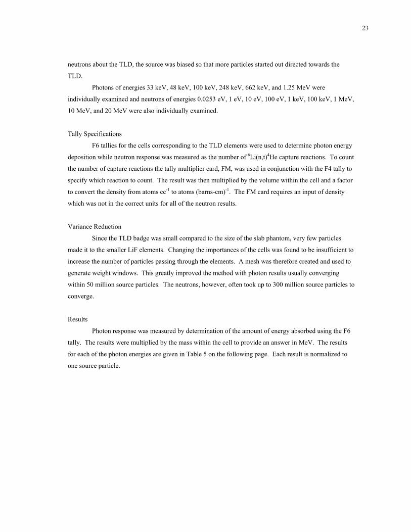
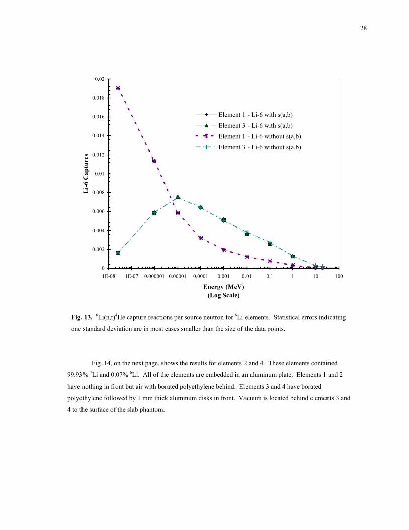
Fig. 13, on the next page, shows the results for elements 1 and 3. These elements contained
95.6% 6Li and 4.4% 7Li. All of the elements are embedded in an aluminum plate. Elements 1 and 2 have
nothing in front but air with borated polyethylene behind. Elements 3 and 4 have borated polyethylene
followed by 1 mm thick aluminum disks in front. These elements have a vacuum behind them.
28
0
0.002
0.004
0.006
0.008
0.01
0.012
0.014
0.016
0.018
0.02
1E-08 1E-07 0.000001 0.00001 0.0001 0.001 0.01 0.1 1 10 100
Energy (MeV)(Log Scale)
Li-6
Cap
ture
s
Element 1 - Li-6 with s(a,b)Element 3 - Li-6 with s(a,b)Element 1 - Li-6 without s(a,b)Element 3 - Li-6 without s(a,b)
Fig. 13. 6Li(n,t)4He capture reactions per source neutron for 6Li elements. Statistical errors indicating
one standard deviation are in most cases smaller than the size of the data points.
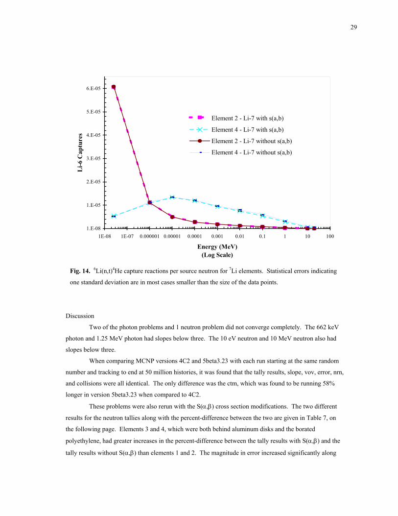
Fig. 14, on the next page, shows the results for elements 2 and 4. These elements contained
99.93% 7Li and 0.07% 6Li. All of the elements are embedded in an aluminum plate. Elements 1 and 2
have nothing in front but air with borated polyethylene behind. Elements 3 and 4 have borated
polyethylene followed by 1 mm thick aluminum disks in front. Vacuum is located behind elements 3 and
4 to the surface of the slab phantom.
29
1.E-08
1.E-05
2.E-05
3.E-05
4.E-05
5.E-05
6.E-05
1E-08 1E-07 0.000001 0.00001 0.0001 0.001 0.01 0.1 1 10 100
Energy (MeV)(Log Scale)
Li-6
Cap
ture
s
Element 2 - Li-7 with s(a,b)
Element 4 - Li-7 with s(a,b)
Element 2 - Li-7 without s(a,b)
Element 4 - Li-7 without s(a,b)
Fig. 14. 6Li(n,t)4He capture reactions per source neutron for 7Li elements. Statistical errors indicating
one standard deviation are in most cases smaller than the size of the data points.
Discussion
Two of the photon problems and 1 neutron problem did not converge completely. The 662 keV
photon and 1.25 MeV photon had slopes below three. The 10 eV neutron and 10 MeV neutron also had
slopes below three.
When comparing MCNP versions 4C2 and 5beta3.23 with each run starting at the same random
number and tracking to end at 50 million histories, it was found that the tally results, slope, vov, error, nrn,
and collisions were all identical. The only difference was the ctm, which was found to be running 58%
longer in version 5beta3.23 when compared to 4C2.
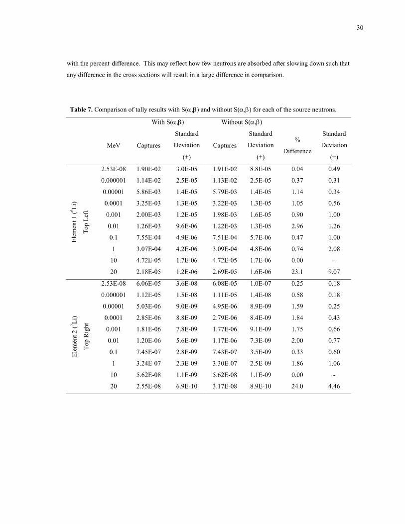
These problems were also rerun with the S(α,β) cross section modifications. The two different
results for the neutron tallies along with the percent-difference between the two are given in Table 7, on
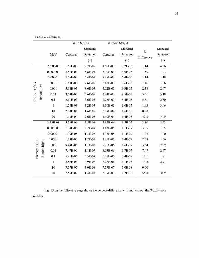
the following page. Elements 3 and 4, which were both behind aluminum disks and the borated
polyethylene, had greater increases in the percent-difference between the tally results with S(α,β) and the
tally results without S(α,β) than elements 1 and 2. The magnitude in error increased significantly along
30
with the percent-difference. This may reflect how few neutrons are absorbed after slowing down such that
any difference in the cross sections will result in a large difference in comparison.
Table 7. Comparison of tally results with S(α,β) and without S(α,β) for each of the source neutrons.
With S(α,β) Without S(α,β)
MeV Captures
Standard
Deviation
(±)
Captures
Standard
Deviation
(±)
%
Difference
Standard
Deviation
(±)
2.53E-08 1.90E-02 3.0E-05 1.91E-02 8.8E-05 0.04 0.49
0.000001 1.14E-02 2.5E-05 1.13E-02 2.5E-05 0.37 0.31
0.00001 5.86E-03 1.4E-05 5.79E-03 1.4E-05 1.14 0.34
0.0001 3.25E-03 1.3E-05 3.22E-03 1.3E-05 1.05 0.56
0.001 2.00E-03 1.2E-05 1.98E-03 1.6E-05 0.90 1.00
0.01 1.26E-03 9.6E-06 1.22E-03 1.3E-05 2.96 1.26
0.1 7.55E-04 4.9E-06 7.51E-04 5.7E-06 0.47 1.00
1 3.07E-04 4.2E-06 3.09E-04 4.8E-06 0.74 2.08
10 4.72E-05 1.7E-06 4.72E-05 1.7E-06 0.00 -
Elem
ent 1
(6 Li)
Top
Left
20 2.18E-05 1.2E-06 2.69E-05 1.6E-06 23.1 9.07
2.53E-08 6.06E-05 3.6E-08 6.08E-05 1.0E-07 0.25 0.18
0.000001 1.12E-05 1.5E-08 1.11E-05 1.4E-08 0.58 0.18
0.00001 5.03E-06 9.0E-09 4.95E-06 8.9E-09 1.59 0.25
0.0001 2.85E-06 8.8E-09 2.79E-06 8.4E-09 1.84 0.43
0.001 1.81E-06 7.8E-09 1.77E-06 9.1E-09 1.75 0.66
0.01 1.20E-06 5.6E-09 1.17E-06 7.3E-09 2.00 0.77
0.1 7.45E-07 2.8E-09 7.43E-07 3.5E-09 0.33 0.60
1 3.24E-07 2.3E-09 3.30E-07 2.5E-09 1.86 1.06
10 5.62E-08 1.1E-09 5.62E-08 1.1E-09 0.00 -
Elem
ent 2
(7 Li)
Top
Rig
ht
20 2.55E-08 6.9E-10 3.17E-08 8.9E-10 24.0 4.46
31
Table 7. Continued. With S(α,β) Without S(α,β)
MeV Captures
Standard
Deviation
(±)
Captures
Standard
Deviation
(±)
%
Difference
Standard
Deviation
(±)
2.53E-08 1.66E-03 2.7E-05 1.68E-03 7.2E-05 1.14 4.66
0.000001 5.81E-03 5.8E-05 5.90E-03 6.0E-05 1.53 1.43
0.00001 7.56E-03 6.4E-05 7.48E-03 6.4E-05 1.14 1.19
0.0001 6.50E-03 7.6E-05 6.41E-03 7.6E-05 1.46 1.66
0.001 5.14E-03 8.6E-05 5.02E-03 9.3E-05 2.38 2.47
0.01 3.64E-03 6.6E-05 3.84E-03 9.5E-05 5.51 3.18
0.1 2.61E-03 3.6E-05 2.76E-03 5.4E-05 5.81 2.50
1 1.28E-03 3.2E-05 1.30E-03 3.0E-05 1.93 3.46
10 2.79E-04 1.6E-05 2.79E-04 1.6E-05 0.00 -
Elem
ent 3
(6 Li)
Bot
tom
Lef
t
20 1.18E-04 9.6E-06 1.69E-04 1.4E-05 42.3 14.55
2.53E-08 5.33E-06 5.5E-08 5.12E-06 1.5E-07 3.89 2.93
0.000001 1.09E-05 9.7E-08 1.13E-05 1.1E-07 3.65 1.35
0.00001 1.33E-05 1.1E-07 1.35E-05 1.1E-07 1.08 1.20
0.0001 1.19E-05 1.2E-07 1.21E-05 1.4E-07 2.08 1.56
0.001 9.43E-06 1.1E-07 9.75E-06 1.6E-07 3.34 2.09
0.01 7.47E-06 1.1E-07 8.03E-06 1.7E-07 7.47 2.67
0.1 5.41E-06 5.5E-08 6.01E-06 7.4E-08 11.1 1.71
1 2.89E-06 4.9E-08 3.28E-06 6.1E-08 13.5 2.71
10 7.27E-07 3.0E-08 7.27E-07 3.0E-08 0.00 -
Elem
ent 4
(7 Li)
Bot
tom
Rig
ht
20 2.56E-07 1.4E-08 3.99E-07 2.2E-08 55.8 10.78
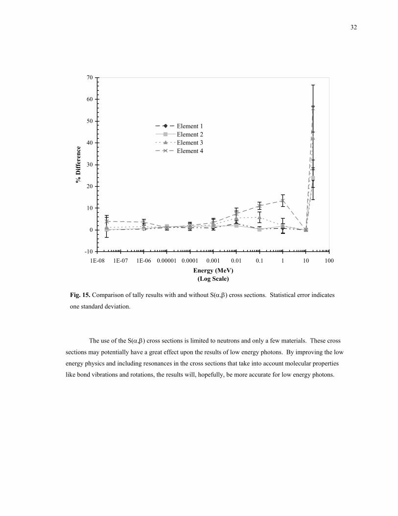
Fig. 15 on the following page shows the percent-difference with and without the S(α,β) cross
sections.
32
-10
0
10
20
30
40
50
60
70
1E-08 1E-07 1E-06 0.00001 0.0001 0.001 0.01 0.1 1 10 100
Energy (MeV)(Log Scale)
% D
iffer
ence
Element 1Element 2Element 3Element 4
Fig. 15. Comparison of tally results with and without S(α,β) cross sections. Statistical error indicates
one standard deviation.
The use of the S(α,β) cross sections is limited to neutrons and only a few materials. These cross
sections may potentially have a great effect upon the results of low energy photons. By improving the low
energy physics and including resonances in the cross sections that take into account molecular properties
like bond vibrations and rotations, the results will, hopefully, be more accurate for low energy photons.
33
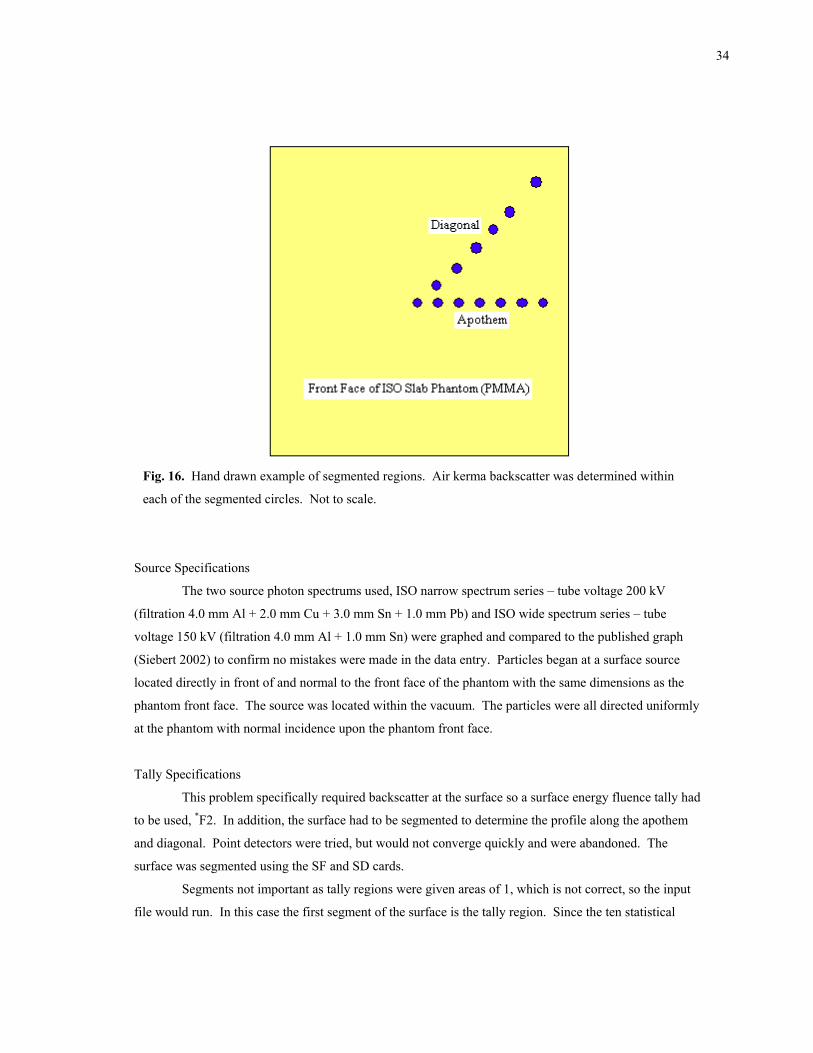
PROBLEM FIVE: AIR KERMA BACKSCATTER PROFILES FOR TWO ISO
PHOTON EXPANDED AND ALIGNED FIELDS IMPINGING ON AN ISO SLAB
PHANTOM
Description of Problem
Air kerma backscatter profiles along the apothem and diagonal of an ISO slab phantom were
determined on the front face of the phantom using a beta version of MCNP 5. This version did not include
the Doppler broadening feature. Two source photon spectra were used. The first was an ISO narrow
spectrum series – tube voltage 200 kV (filtration 4.0 mm Al + 2.0 mm Cu + 3.0 mm Sn + 1.0 mm Pb).
The second was an ISO wide spectrum series – tube voltage 150 kV (filtration 4.0 mm Al + 1.0 mm Sn).
The air kerma backscatter profiles were determined along the diagonal and apothem on the front face.
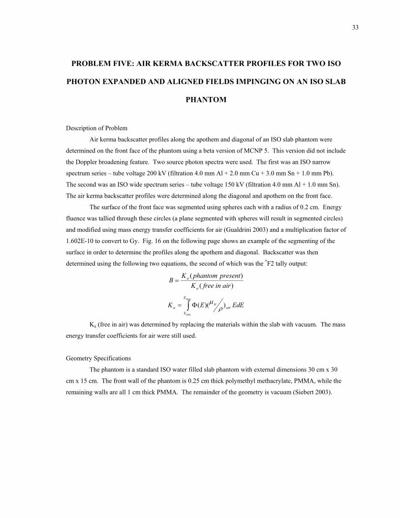
The surface of the front face was segmented using spheres each with a radius of 0.2 cm. Energy
fluence was tallied through these circles (a plane segmented with spheres will result in segmented circles)
and modified using mass energy transfer coefficients for air (Gualdrini 2003) and a multiplication factor of
1.602E-10 to convert to Gy. Fig. 16 on the following page shows an example of the segmenting of the
surface in order to determine the profiles along the apothem and diagonal. Backscatter was then
determined using the following two equations, the second of which was the *F2 tally output:
)()(
airinfreeKpresentphantomKB
a
a=
∫ Φ=max
min
))((E
Eair
tra EdEEK ρ
µ
Ka (free in air) was determined by replacing the materials within the slab with vacuum. The mass
energy transfer coefficients for air were still used.
Geometry Specifications
The phantom is a standard ISO water filled slab phantom with external dimensions 30 cm x 30
cm x 15 cm. The front wall of the phantom is 0.25 cm thick polymethyl methacrylate, PMMA, while the
remaining walls are all 1 cm thick PMMA. The remainder of the geometry is vacuum (Siebert 2003).
34
Fig. 16. Hand drawn example of segmented regions. Air kerma backscatter was determined within
each of the segmented circles. Not to scale.
Source Specifications
The two source photon spectrums used, ISO narrow spectrum series – tube voltage 200 kV
(filtration 4.0 mm Al + 2.0 mm Cu + 3.0 mm Sn + 1.0 mm Pb) and ISO wide spectrum series – tube
voltage 150 kV (filtration 4.0 mm Al + 1.0 mm Sn) were graphed and compared to the published graph
(Siebert 2002) to confirm no mistakes were made in the data entry. Particles began at a surface source
located directly in front of and normal to the front face of the phantom with the same dimensions as the
phantom front face. The source was located within the vacuum. The particles were all directed uniformly
at the phantom with normal incidence upon the phantom front face.
Tally Specifications
This problem specifically required backscatter at the surface so a surface energy fluence tally had
to be used, *F2. In addition, the surface had to be segmented to determine the profile along the apothem
and diagonal. Point detectors were tried, but would not converge quickly and were abandoned. The
surface was segmented using the SF and SD cards.
Segments not important as tally regions were given areas of 1, which is not correct, so the input
file would run. In this case the first segment of the surface is the tally region. Since the ten statistical
35
checks performed by MCNP are only performed on the first bin, or segment in this case, this proved to be
a good way to perform the segmentation.
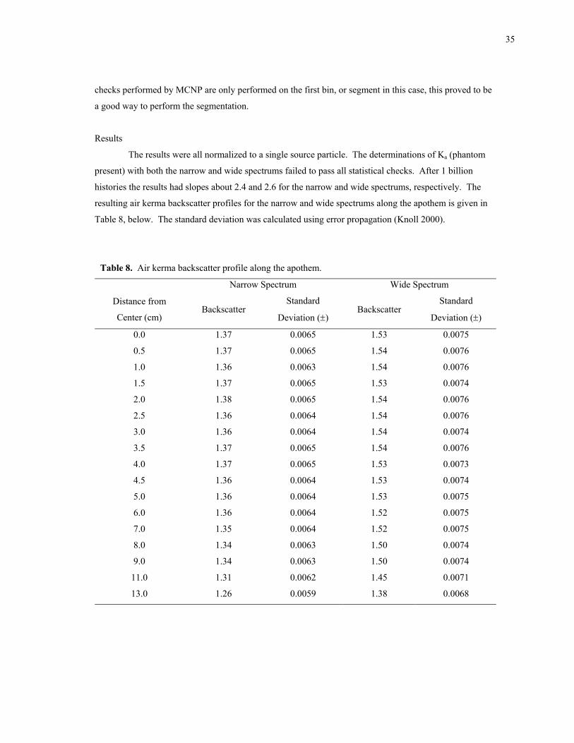
Results
The results were all normalized to a single source particle. The determinations of Ka (phantom
present) with both the narrow and wide spectrums failed to pass all statistical checks. After 1 billion
histories the results had slopes about 2.4 and 2.6 for the narrow and wide spectrums, respectively. The
resulting air kerma backscatter profiles for the narrow and wide spectrums along the apothem is given in
Table 8, below. The standard deviation was calculated using error propagation (Knoll 2000).
Table 8. Air kerma backscatter profile along the apothem.
Narrow Spectrum Wide Spectrum
Distance from
Center (cm) Backscatter
Standard
Deviation (±) Backscatter
Standard
Deviation (±)
0.0 1.37 0.0065 1.53 0.0075
0.5 1.37 0.0065 1.54 0.0076
1.0 1.36 0.0063 1.54 0.0076
1.5 1.37 0.0065 1.53 0.0074
2.0 1.38 0.0065 1.54 0.0076
2.5 1.36 0.0064 1.54 0.0076
3.0 1.36 0.0064 1.54 0.0074
3.5 1.37 0.0065 1.54 0.0076
4.0 1.37 0.0065 1.53 0.0073
4.5 1.36 0.0064 1.53 0.0074
5.0 1.36 0.0064 1.53 0.0075
6.0 1.36 0.0064 1.52 0.0075
7.0 1.35 0.0064 1.52 0.0075
8.0 1.34 0.0063 1.50 0.0074
9.0 1.34 0.0063 1.50 0.0074
11.0 1.31 0.0062 1.45 0.0071
13.0 1.26 0.0059 1.38 0.0068
36
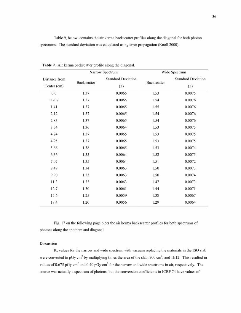
Table 9, below, contains the air kerma backscatter profiles along the diagonal for both photon
spectrums. The standard deviation was calculated using error propagation (Knoll 2000).
Table 9. Air kerma backscatter profile along the diagonal.
Narrow Spectrum Wide Spectrum
Distance from
Center (cm) Backscatter
Standard Deviation
(±) Backscatter
Standard Deviation
(±)
0.0 1.37 0.0065 1.53 0.0075
0.707 1.37 0.0065 1.54 0.0076
1.41 1.37 0.0065 1.55 0.0076
2.12 1.37 0.0065 1.54 0.0076
2.83 1.37 0.0065 1.54 0.0076
3.54 1.36 0.0064 1.53 0.0075
4.24 1.37 0.0065 1.53 0.0075
4.95 1.37 0.0065 1.53 0.0075
5.66 1.38 0.0065 1.53 0.0074
6.36 1.35 0.0064 1.52 0.0075
7.07 1.35 0.0064 1.51 0.0072
8.49 1.34 0.0063 1.50 0.0073
9.90 1.33 0.0063 1.50 0.0074
11.3 1.33 0.0063 1.47 0.0073
12.7 1.30 0.0061 1.44 0.0071
15.6 1.25 0.0059 1.38 0.0067
18.4 1.20 0.0056 1.29 0.0064
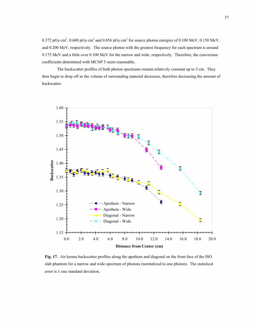
Fig. 17 on the following page plots the air kerma backscatter profiles for both spectrums of
photons along the apothem and diagonal.
Discussion
Ka values for the narrow and wide spectrum with vacuum replacing the materials in the ISO slab
were converted to pGy⋅cm2 by multiplying times the area of the slab, 900 cm2, and 1E12. This resulted in
values of 0.675 pGy⋅cm2 and 0.40 pGy⋅cm2 for the narrow and wide spectrums in air, respectively. The
source was actually a spectrum of photons, but the conversion coefficients in ICRP 74 have values of
37
0.372 pGy⋅cm2, 0.600 pGy⋅cm2 and 0.856 pGy⋅cm2 for source photon energies of 0.100 MeV, 0.150 MeV,
and 0.200 MeV, respectively. The source photon with the greatest frequency for each spectrum is around
0.175 MeV and a little over 0.100 MeV for the narrow and wide, respectively. Therefore, the conversion
coefficients determined with MCNP 5 seem reasonable.
The backscatter profiles of both photon spectrums remain relatively constant up to 5 cm. They
then begin to drop off as the volume of surrounding material decreases, therefore decreasing the amount of
backscatter.
1.15
1.20
1.25
1.30
1.35
1.40
1.45
1.50
1.55
1.60
0.0 2.0 4.0 6.0 8.0 10.0 12.0 14.0 16.0 18.0 20.0
Distance from Center (cm)
Bac
ksca
tter
Apothem - NarrowApothem - WideDiagonal - NarrowDiagonal - Wide
Fig. 17. Air kerma backscatter profiles along the apothem and diagonal on the front face of the ISO
slab phantom for a narrow and wide spectrum of photons (normalized to one photon). The statistical
error is ± one standard deviation.
38
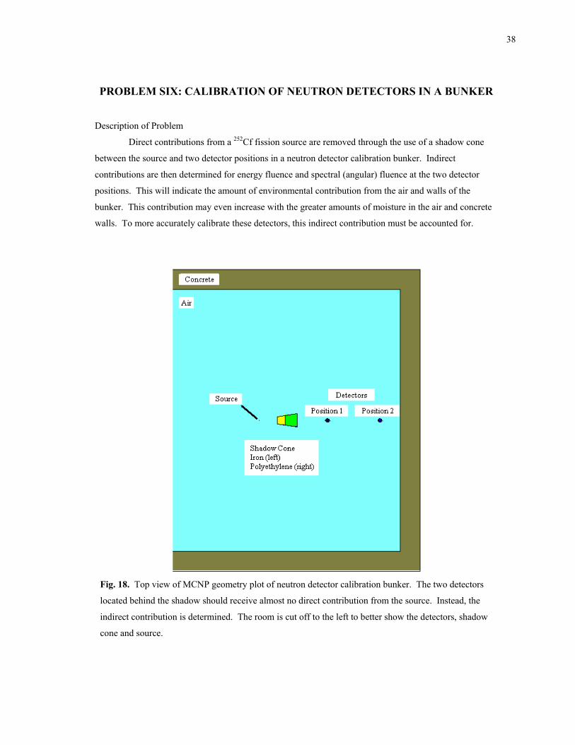
PROBLEM SIX: CALIBRATION OF NEUTRON DETECTORS IN A BUNKER
Description of Problem
Direct contributions from a 252Cf fission source are removed through the use of a shadow cone
between the source and two detector positions in a neutron detector calibration bunker. Indirect
contributions are then determined for energy fluence and spectral (angular) fluence at the two detector
positions. This will indicate the amount of environmental contribution from the air and walls of the
bunker. This contribution may even increase with the greater amounts of moisture in the air and concrete
walls. To more accurately calibrate these detectors, this indirect contribution must be accounted for.
Fig. 18. Top view of MCNP geometry plot of neutron detector calibration bunker. The two detectors
located behind the shadow should receive almost no direct contribution from the source. Instead, the
indirect contribution is determined. The room is cut off to the left to better show the detectors, shadow
cone and source.
39
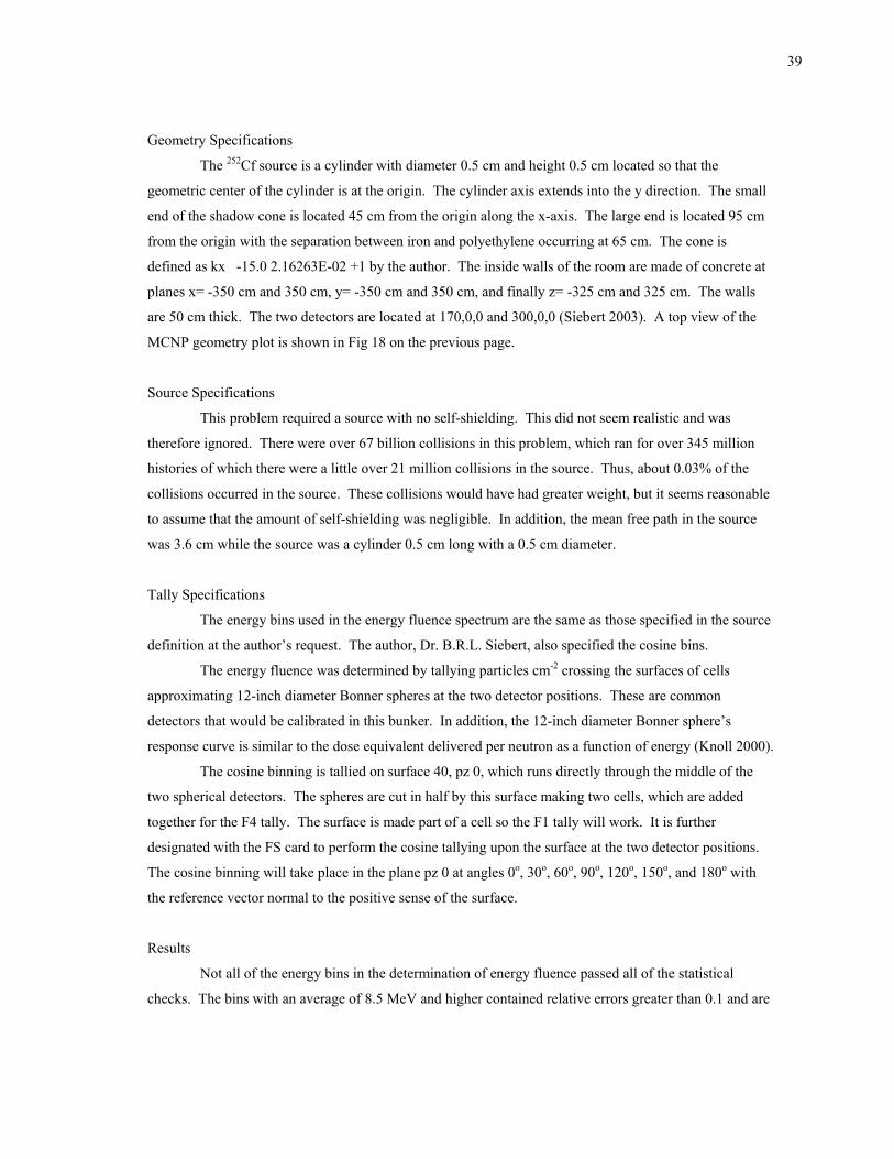
Geometry Specifications
The 252Cf source is a cylinder with diameter 0.5 cm and height 0.5 cm located so that the
geometric center of the cylinder is at the origin. The cylinder axis extends into the y direction. The small
end of the shadow cone is located 45 cm from the origin along the x-axis. The large end is located 95 cm
from the origin with the separation between iron and polyethylene occurring at 65 cm. The cone is
defined as kx -15.0 2.16263E-02 +1 by the author. The inside walls of the room are made of concrete at
planes x= -350 cm and 350 cm, y= -350 cm and 350 cm, and finally z= -325 cm and 325 cm. The walls
are 50 cm thick. The two detectors are located at 170,0,0 and 300,0,0 (Siebert 2003). A top view of the
MCNP geometry plot is shown in Fig 18 on the previous page.
Source Specifications
This problem required a source with no self-shielding. This did not seem realistic and was
therefore ignored. There were over 67 billion collisions in this problem, which ran for over 345 million
histories of which there were a little over 21 million collisions in the source. Thus, about 0.03% of the
collisions occurred in the source. These collisions would have had greater weight, but it seems reasonable
to assume that the amount of self-shielding was negligible. In addition, the mean free path in the source
was 3.6 cm while the source was a cylinder 0.5 cm long with a 0.5 cm diameter.
Tally Specifications
The energy bins used in the energy fluence spectrum are the same as those specified in the source
definition at the author’s request. The author, Dr. B.R.L. Siebert, also specified the cosine bins.
The energy fluence was determined by tallying particles cm-2 crossing the surfaces of cells
approximating 12-inch diameter Bonner spheres at the two detector positions. These are common
detectors that would be calibrated in this bunker. In addition, the 12-inch diameter Bonner sphere’s
response curve is similar to the dose equivalent delivered per neutron as a function of energy (Knoll 2000).
The cosine binning is tallied on surface 40, pz 0, which runs directly through the middle of the
two spherical detectors. The spheres are cut in half by this surface making two cells, which are added
together for the F4 tally. The surface is made part of a cell so the F1 tally will work. It is further
designated with the FS card to perform the cosine tallying upon the surface at the two detector positions.
The cosine binning will take place in the plane pz 0 at angles 0o, 30o, 60o, 90o, 120o, 150o, and 180o with
the reference vector normal to the positive sense of the surface.
Results
Not all of the energy bins in the determination of energy fluence passed all of the statistical
checks. The bins with an average of 8.5 MeV and higher contained relative errors greater than 0.1 and are
40
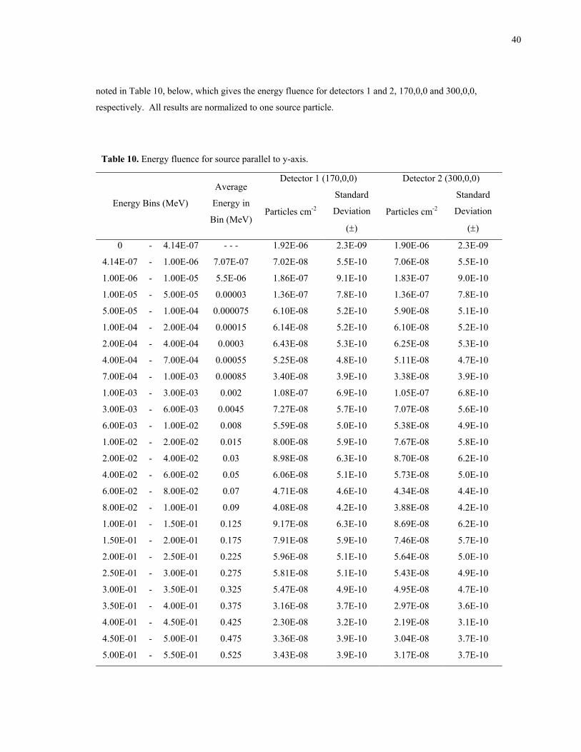
noted in Table 10, below, which gives the energy fluence for detectors 1 and 2, 170,0,0 and 300,0,0,
respectively. All results are normalized to one source particle.
Table 10. Energy fluence for source parallel to y-axis.
Detector 1 (170,0,0) Detector 2 (300,0,0)
Energy Bins (MeV)
Average
Energy in
Bin (MeV) Particles cm-2
Standard
Deviation
(±)
Particles cm-2
Standard
Deviation
(±)
0 - 4.14E-07 - - - 1.92E-06 2.3E-09 1.90E-06 2.3E-09
4.14E-07 - 1.00E-06 7.07E-07 7.02E-08 5.5E-10 7.06E-08 5.5E-10
1.00E-06 - 1.00E-05 5.5E-06 1.86E-07 9.1E-10 1.83E-07 9.0E-10
1.00E-05 - 5.00E-05 0.00003 1.36E-07 7.8E-10 1.36E-07 7.8E-10
5.00E-05 - 1.00E-04 0.000075 6.10E-08 5.2E-10 5.90E-08 5.1E-10
1.00E-04 - 2.00E-04 0.00015 6.14E-08 5.2E-10 6.10E-08 5.2E-10
2.00E-04 - 4.00E-04 0.0003 6.43E-08 5.3E-10 6.25E-08 5.3E-10
4.00E-04 - 7.00E-04 0.00055 5.25E-08 4.8E-10 5.11E-08 4.7E-10
7.00E-04 - 1.00E-03 0.00085 3.40E-08 3.9E-10 3.38E-08 3.9E-10
1.00E-03 - 3.00E-03 0.002 1.08E-07 6.9E-10 1.05E-07 6.8E-10
3.00E-03 - 6.00E-03 0.0045 7.27E-08 5.7E-10 7.07E-08 5.6E-10
6.00E-03 - 1.00E-02 0.008 5.59E-08 5.0E-10 5.38E-08 4.9E-10
1.00E-02 - 2.00E-02 0.015 8.00E-08 5.9E-10 7.67E-08 5.8E-10
2.00E-02 - 4.00E-02 0.03 8.98E-08 6.3E-10 8.70E-08 6.2E-10
4.00E-02 - 6.00E-02 0.05 6.06E-08 5.1E-10 5.73E-08 5.0E-10
6.00E-02 - 8.00E-02 0.07 4.71E-08 4.6E-10 4.34E-08 4.4E-10
8.00E-02 - 1.00E-01 0.09 4.08E-08 4.2E-10 3.88E-08 4.2E-10
1.00E-01 - 1.50E-01 0.125 9.17E-08 6.3E-10 8.69E-08 6.2E-10
1.50E-01 - 2.00E-01 0.175 7.91E-08 5.9E-10 7.46E-08 5.7E-10
2.00E-01 - 2.50E-01 0.225 5.96E-08 5.1E-10 5.64E-08 5.0E-10
2.50E-01 - 3.00E-01 0.275 5.81E-08 5.1E-10 5.43E-08 4.9E-10
3.00E-01 - 3.50E-01 0.325 5.47E-08 4.9E-10 4.95E-08 4.7E-10
3.50E-01 - 4.00E-01 0.375 3.16E-08 3.7E-10 2.97E-08 3.6E-10
4.00E-01 - 4.50E-01 0.425 2.30E-08 3.2E-10 2.19E-08 3.1E-10
4.50E-01 - 5.00E-01 0.475 3.36E-08 3.9E-10 3.04E-08 3.7E-10
5.00E-01 - 5.50E-01 0.525 3.43E-08 3.9E-10 3.17E-08 3.7E-10
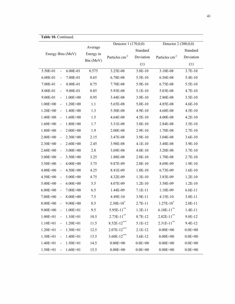
41
Table 10. Continued.
Detector 1 (170,0,0) Detector 2 (300,0,0)
Energy Bins (MeV)
Average
Energy in
Bin (MeV) Particles cm-2
Standard
Deviation
(±)
Particles cm-2
Standard
Deviation
(±)
5.50E-01 - 6.00E-01 0.575 3.25E-08 3.8E-10 3.10E-08 3.7E-10
6.00E-01 - 7.00E-01 0.65 6.78E-08 5.5E-10 6.56E-08 5.4E-10
7.00E-01 - 8.00E-01 0.75 7.70E-08 5.9E-10 6.75E-08 5.5E-10
8.00E-01 - 9.00E-01 0.85 5.93E-08 5.1E-10 5.03E-08 4.7E-10
9.00E-01 - 1.00E+00 0.95 3.44E-08 3.9E-10 2.80E-08 3.5E-10
1.00E+00 - 1.20E+00 1.1 5.65E-08 5.0E-10 4.85E-08 4.6E-10
1.20E+00 - 1.40E+00 1.3 5.50E-08 4.9E-10 4.68E-08 4.5E-10
1.40E+00 - 1.60E+00 1.5 4.64E-08 4.5E-10 4.00E-08 4.2E-10
1.60E+00 - 1.80E+00 1.7 3.31E-08 3.8E-10 2.84E-08 3.5E-10
1.80E+00 - 2.00E+00 1.9 2.00E-08 2.9E-10 1.70E-08 2.7E-10
2.00E+00 - 2.30E+00 2.15 3.47E-08 3.9E-10 3.04E-08 3.6E-10
2.30E+00 - 2.60E+00 2.45 3.98E-08 4.1E-10 3.48E-08 3.9E-10
2.60E+00 - 3.00E+00 2.8 3.69E-08 4.0E-10 3.20E-08 3.7E-10
3.00E+00 - 3.50E+00 3.25 1.88E-08 2.8E-10 1.78E-08 2.7E-10
3.50E+00 - 4.00E+00 3.75 9.87E-09 2.0E-10 8.69E-09 1.9E-10
4.00E+00 - 4.50E+00 4.25 8.41E-09 1.8E-10 6.73E-09 1.6E-10
4.50E+00 - 5.00E+00 4.75 4.32E-09 1.3E-10 3.83E-09 1.2E-10
5.00E+00 - 6.00E+00 5.5 4.07E-09 1.2E-10 3.58E-09 1.2E-10
6.00E+00 - 7.00E+00 6.5 1.44E-09 7.1E-11 1.18E-09 6.6E-11
7.00E+00 - 8.00E+00 7.5 4.49E-10 3.9E-11 4.15E-10 3.8E-11
8.00E+00 - 9.00E+00 8.5 2.30E-10* 2.7E-11 1.27E-10* 2.0E-11
9.00E+00 - 1.00E+01 9.5 5.95E-11** 1.3E-11 6.10E-11** 1.4E-11
1.00E+01 - 1.10E+01 10.5 2.73E-11** 8.7E-12 2.82E-11** 9.8E-12
1.10E+01 - 1.20E+01 11.5 8.52E-12*** 5.1E-12 2.31E-11** 9.4E-12
1.20E+01 - 1.30E+01 12.5 2.07E-12*** 2.1E-12 0.00E+00 0.0E+00
1.30E+01 - 1.40E+01 13.5 3.60E-12*** 3.6E-12 0.00E+00 0.0E+00
1.40E+01 - 1.50E+01 14.5 0.00E+00 0.0E+00 0.00E+00 0.0E+00
1.50E+01 - 1.60E+01 15.5 0.00E+00 0.0E+00 0.00E+00 0.0E+00
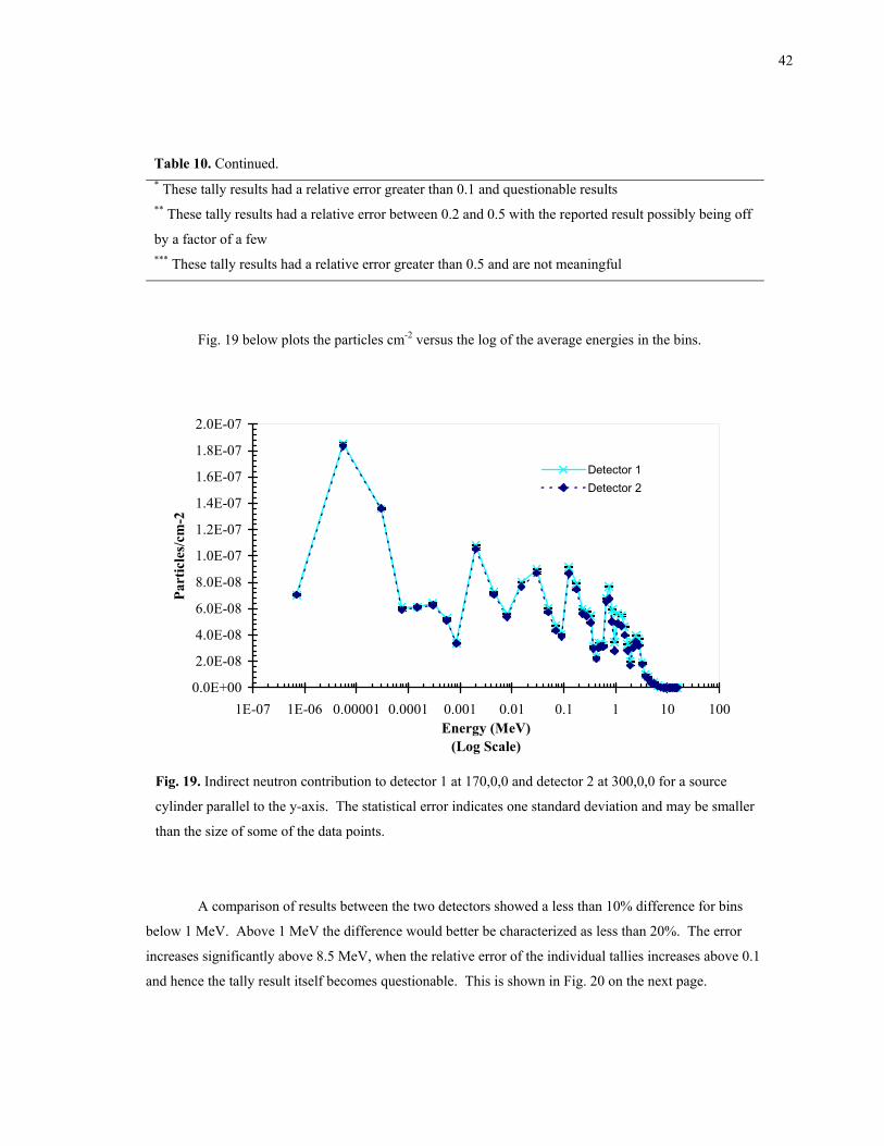
42
Table 10. Continued. * These tally results had a relative error greater than 0.1 and questionable results ** These tally results had a relative error between 0.2 and 0.5 with the reported result possibly being off
by a factor of a few *** These tally results had a relative error greater than 0.5 and are not meaningful
Fig. 19 below plots the particles cm-2 versus the log of the average energies in the bins.
0.0E+00
2.0E-08
4.0E-08
6.0E-08
8.0E-08
1.0E-07
1.2E-07
1.4E-07
1.6E-07
1.8E-07
2.0E-07
1E-07 1E-06 0.00001 0.0001 0.001 0.01 0.1 1 10 100Energy (MeV)
(Log Scale)
Part
icle
s/cm
-2
Detector 1Detector 2
Fig. 19. Indirect neutron contribution to detector 1 at 170,0,0 and detector 2 at 300,0,0 for a source
cylinder parallel to the y-axis. The statistical error indicates one standard deviation and may be smaller
than the size of some of the data points.
A comparison of results between the two detectors showed a less than 10% difference for bins
below 1 MeV. Above 1 MeV the difference would better be characterized as less than 20%. The error
increases significantly above 8.5 MeV, when the relative error of the individual tallies increases above 0.1
and hence the tally result itself becomes questionable. This is shown in Fig. 20 on the next page.
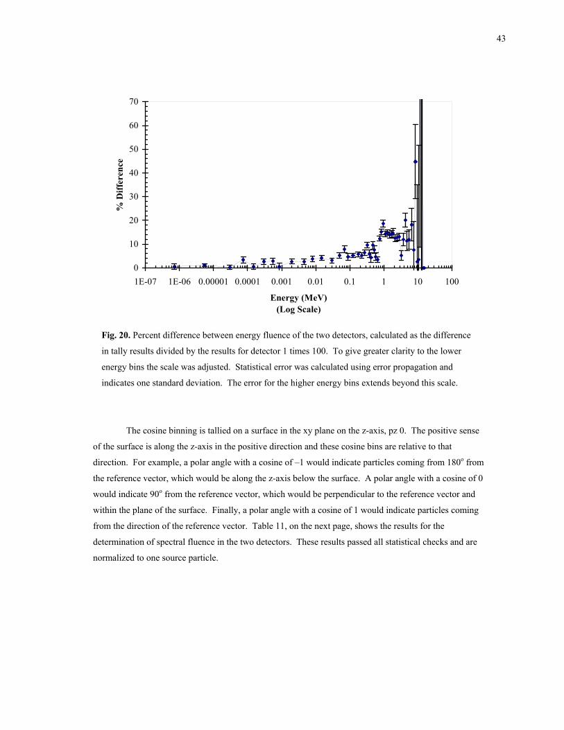
43
0
10
20
30
40
50
60
70
1E-07 1E-06 0.00001 0.0001 0.001 0.01 0.1 1 10 100
Energy (MeV)(Log Scale)
% D
iffer
ence
Fig. 20. Percent difference between energy fluence of the two detectors, calculated as the difference
in tally results divided by the results for detector 1 times 100. To give greater clarity to the lower
energy bins the scale was adjusted. Statistical error was calculated using error propagation and
indicates one standard deviation. The error for the higher energy bins extends beyond this scale.
The cosine binning is tallied on a surface in the xy plane on the z-axis, pz 0. The positive sense
of the surface is along the z-axis in the positive direction and these cosine bins are relative to that
direction. For example, a polar angle with a cosine of –1 would indicate particles coming from 180o from
the reference vector, which would be along the z-axis below the surface. A polar angle with a cosine of 0
would indicate 90o from the reference vector, which would be perpendicular to the reference vector and
within the plane of the surface. Finally, a polar angle with a cosine of 1 would indicate particles coming
from the direction of the reference vector. Table 11, on the next page, shows the results for the
determination of spectral fluence in the two detectors. These results passed all statistical checks and are
normalized to one source particle.
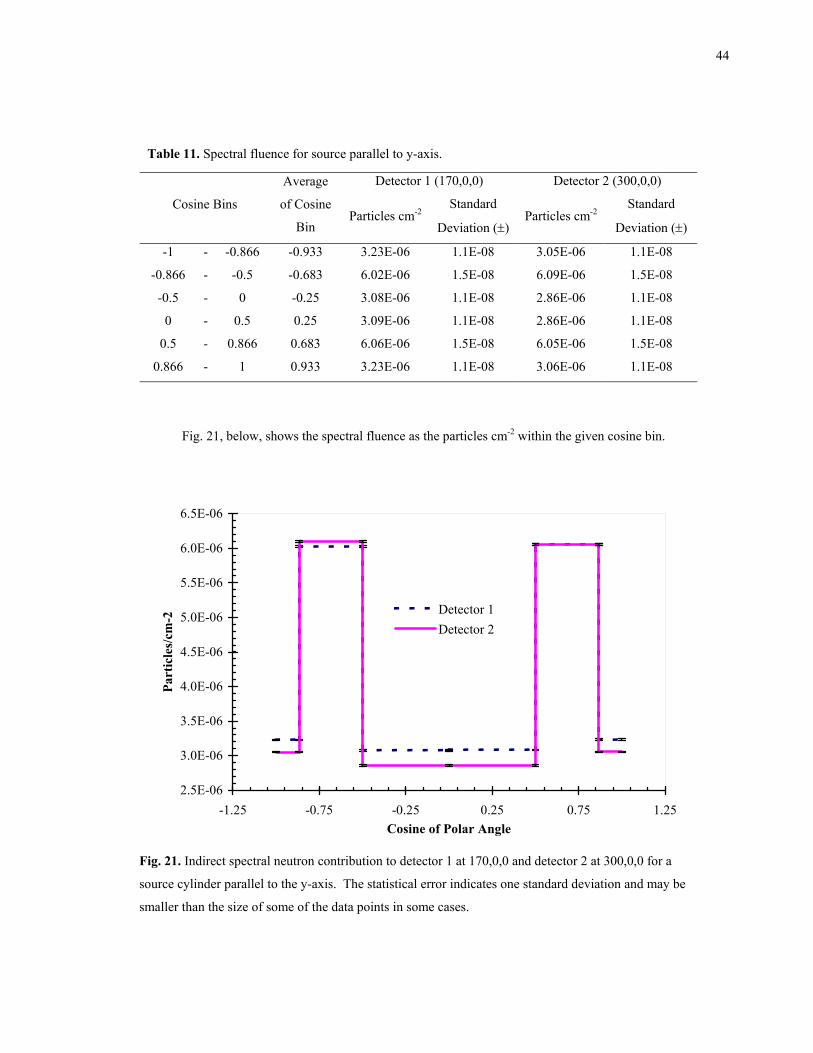
44
Table 11. Spectral fluence for source parallel to y-axis.
Detector 1 (170,0,0) Detector 2 (300,0,0)
Cosine Bins
Average
of Cosine
Bin Particles cm-2
Standard
Deviation (±) Particles cm-2
Standard
Deviation (±)
-1 - -0.866 -0.933 3.23E-06 1.1E-08 3.05E-06 1.1E-08
-0.866 - -0.5 -0.683 6.02E-06 1.5E-08 6.09E-06 1.5E-08
-0.5 - 0 -0.25 3.08E-06 1.1E-08 2.86E-06 1.1E-08
0 - 0.5 0.25 3.09E-06 1.1E-08 2.86E-06 1.1E-08
0.5 - 0.866 0.683 6.06E-06 1.5E-08 6.05E-06 1.5E-08
0.866 - 1 0.933 3.23E-06 1.1E-08 3.06E-06 1.1E-08
Fig. 21, below, shows the spectral fluence as the particles cm-2 within the given cosine bin.
2.5E-06
3.0E-06
3.5E-06
4.0E-06
4.5E-06
5.0E-06
5.5E-06
6.0E-06
6.5E-06
-1.25 -0.75 -0.25 0.25 0.75 1.25Cosine of Polar Angle
Part
icle
s/cm
-2
Detector 1Detector 2
Fig. 21. Indirect spectral neutron contribution to detector 1 at 170,0,0 and detector 2 at 300,0,0 for a
source cylinder parallel to the y-axis. The statistical error indicates one standard deviation and may be
smaller than the size of some of the data points in some cases.

45
Discussion
Indirect contribution seems to be very small with the largest contribution coming from the low
energy neutrons with an average polar angle of 47o relative to particles crossing the surface, pz 0, along
the z-axis from the positive side of the surface.
Source neutrons >0.8 MeV seem to produce a significant difference in indirect neutron
contributions to the two detectors. However, this is also where the tally results began to have a large
relative error, so this may not be true. There is little difference between the two detectors with low energy
source neutrons.
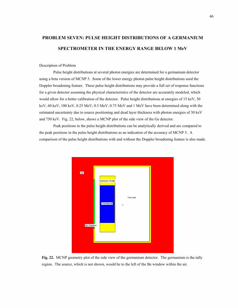
46
PROBLEM SEVEN: PULSE HEIGHT DISTRIBUTIONS OF A GERMANIUM
SPECTROMETER IN THE ENERGY RANGE BELOW 1 MeV
Description of Problem
Pulse height distributions at several photon energies are determined for a germanium detector
using a beta version of MCNP 5. Some of the lower energy photon pulse height distributions used the
Doppler broadening feature. These pulse height distributions may provide a full set of response functions
for a given detector assuming the physical characteristics of the detector are accurately modeled, which
would allow for a better calibration of the detector. Pulse height distributions at energies of 15 keV, 30
keV, 60 keV, 100 keV, 0.25 MeV, 0.5 MeV, 0.75 MeV and 1 MeV have been determined along with the
estimated uncertainty due to source positioning and dead layer thickness with photon energies of 30 keV
and 750 keV. Fig. 22, below, shows a MCNP plot of the side view of the Ge detector.
Peak positions in the pulse height distributions can be analytically derived and are compared to
the peak positions in the pulse height distributions as an indication of the accuracy of MCNP 5. A
comparison of the pulse height distributions with and without the Doppler broadening feature is also made.
Fig. 22. MCNP geometry plot of the side view of the germanium detector. The germanium is the tally
region. The source, which is not shown, would be to the left of the Be window within the air.
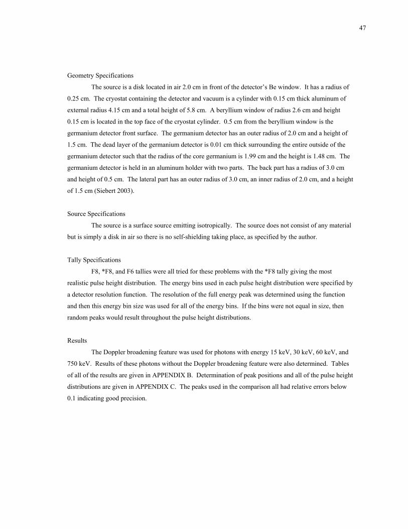
47
Geometry Specifications
The source is a disk located in air 2.0 cm in front of the detector’s Be window. It has a radius of
0.25 cm. The cryostat containing the detector and vacuum is a cylinder with 0.15 cm thick aluminum of
external radius 4.15 cm and a total height of 5.8 cm. A beryllium window of radius 2.6 cm and height
0.15 cm is located in the top face of the cryostat cylinder. 0.5 cm from the beryllium window is the
germanium detector front surface. The germanium detector has an outer radius of 2.0 cm and a height of
1.5 cm. The dead layer of the germanium detector is 0.01 cm thick surrounding the entire outside of the
germanium detector such that the radius of the core germanium is 1.99 cm and the height is 1.48 cm. The
germanium detector is held in an aluminum holder with two parts. The back part has a radius of 3.0 cm
and height of 0.5 cm. The lateral part has an outer radius of 3.0 cm, an inner radius of 2.0 cm, and a height
of 1.5 cm (Siebert 2003).
Source Specifications
The source is a surface source emitting isotropically. The source does not consist of any material
but is simply a disk in air so there is no self-shielding taking place, as specified by the author.
Tally Specifications
F8, *F8, and F6 tallies were all tried for these problems with the *F8 tally giving the most
realistic pulse height distribution. The energy bins used in each pulse height distribution were specified by
a detector resolution function. The resolution of the full energy peak was determined using the function
and then this energy bin size was used for all of the energy bins. If the bins were not equal in size, then
random peaks would result throughout the pulse height distributions.
Results
The Doppler broadening feature was used for photons with energy 15 keV, 30 keV, 60 keV, and
750 keV. Results of these photons without the Doppler broadening feature were also determined. Tables
of all of the results are given in APPENDIX B. Determination of peak positions and all of the pulse height
distributions are given in APPENDIX C. The peaks used in the comparison all had relative errors below
0.1 indicating good precision.
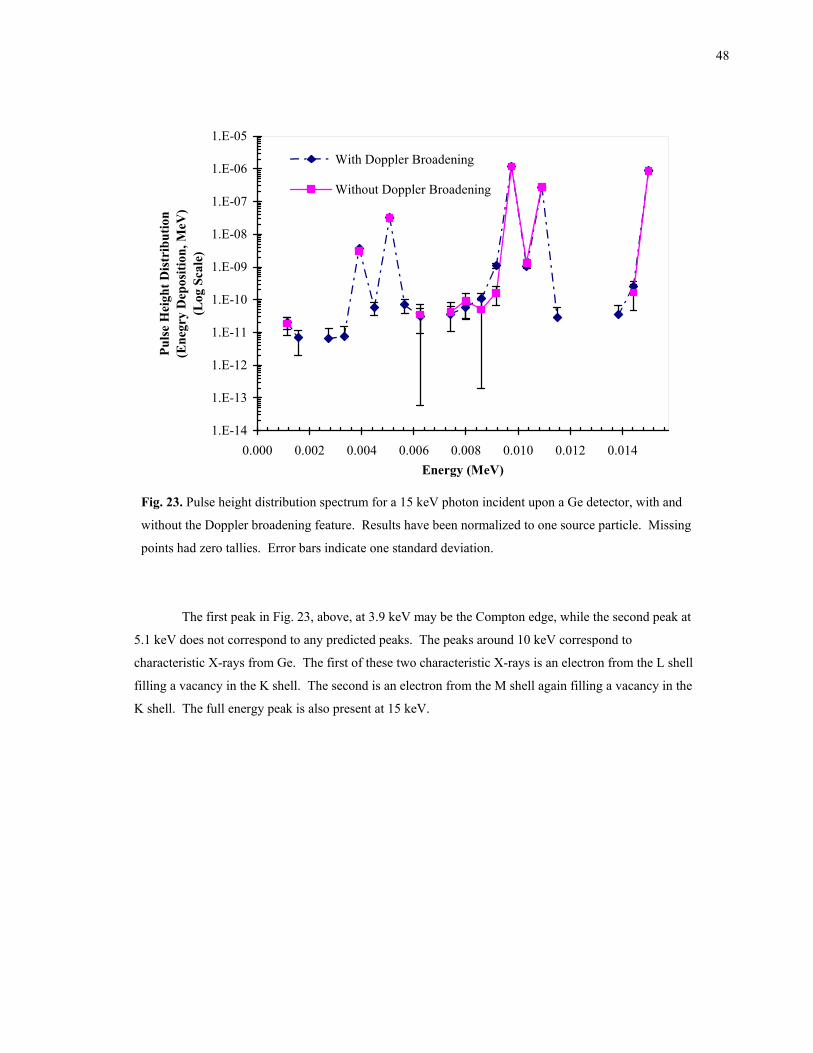
48
1.E-14
1.E-13
1.E-12
1.E-11
1.E-10
1.E-09
1.E-08
1.E-07
1.E-06
1.E-05
0.000 0.002 0.004 0.006 0.008 0.010 0.012 0.014Energy (MeV)
Puls
e H
eigh
t Dis
trib
utio
n(E
negr
y D
epos
ition
, MeV
)(L
og S
cale
)
With Doppler Broadening
Without Doppler Broadening
Fig. 23. Pulse height distribution spectrum for a 15 keV photon incident upon a Ge detector, with and
without the Doppler broadening feature. Results have been normalized to one source particle. Missing
points had zero tallies. Error bars indicate one standard deviation.
The first peak in Fig. 23, above, at 3.9 keV may be the Compton edge, while the second peak at
5.1 keV does not correspond to any predicted peaks. The peaks around 10 keV correspond to
characteristic X-rays from Ge. The first of these two characteristic X-rays is an electron from the L shell
filling a vacancy in the K shell. The second is an electron from the M shell again filling a vacancy in the
K shell. The full energy peak is also present at 15 keV.
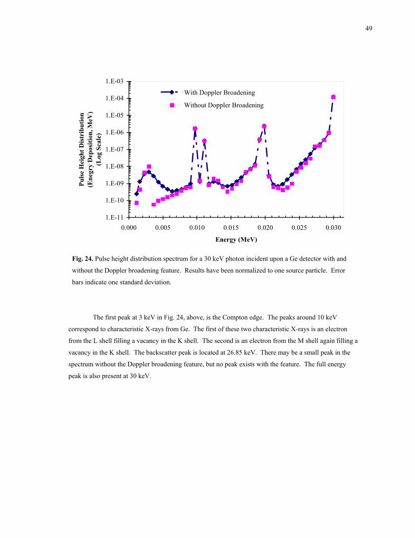
49
1.E-11
1.E-10
1.E-09
1.E-08
1.E-07
1.E-06
1.E-05
1.E-04
1.E-03
0.000 0.005 0.010 0.015 0.020 0.025 0.030
Energy (MeV)
Puls
e H
eigh
t Dis
trib
utio
n(E
negr
y D
epos
ition
, MeV
)(L
og S
cale
)With Doppler Broadening
Without Doppler Broadening
Fig. 24. Pulse height distribution spectrum for a 30 keV photon incident upon a Ge detector with and
without the Doppler broadening feature. Results have been normalized to one source particle. Error
bars indicate one standard deviation.
The first peak at 3 keV in Fig. 24, above, is the Compton edge. The peaks around 10 keV
correspond to characteristic X-rays from Ge. The first of these two characteristic X-rays is an electron
from the L shell filling a vacancy in the K shell. The second is an electron from the M shell again filling a
vacancy in the K shell. The backscatter peak is located at 26.85 keV. There may be a small peak in the
spectrum without the Doppler broadening feature, but no peak exists with the feature. The full energy
peak is also present at 30 keV.
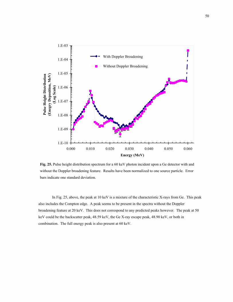
50
1.E-10
1.E-09
1.E-08
1.E-07
1.E-06
1.E-05
1.E-04
1.E-03
0.000 0.010 0.020 0.030 0.040 0.050 0.060
Energy (MeV)
Puls
e H
eigh
t Dis
trib
utio
n(E
negr
y D
epos
ition
, MeV
)(L
og S
cale
)With Doppler Broadening
Without Doppler Broadening
Fig. 25. Pulse height distribution spectrum for a 60 keV photon incident upon a Ge detector with and
without the Doppler broadening feature. Results have been normalized to one source particle. Error
bars indicate one standard deviation.
In Fig. 25, above, the peak at 10 keV is a mixture of the characteristic X-rays from Ge. This peak
also includes the Compton edge. A peak seems to be present in the spectra without the Doppler
broadening feature at 20 keV. This does not correspond to any predicted peaks however. The peak at 50
keV could be the backscatter peak, 48.59 keV, the Ge X-ray escape peak, 48.90 keV, or both in
combination. The full energy peak is also present at 60 keV.
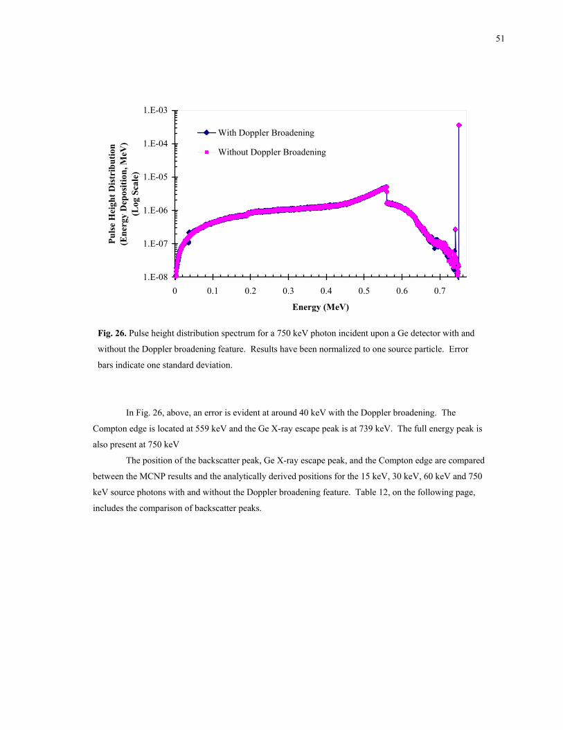
51
1.E-08
1.E-07
1.E-06
1.E-05
1.E-04
1.E-03
0 0.1 0.2 0.3 0.4 0.5 0.6 0.7
Energy (MeV)
Puls
e H
eigh
t Dis
trib
utio
n(E
nerg
y D
epos
ition
, MeV
)(L
og S
cale
)With Doppler Broadening
Without Doppler Broadening
Fig. 26. Pulse height distribution spectrum for a 750 keV photon incident upon a Ge detector with and
without the Doppler broadening feature. Results have been normalized to one source particle. Error
bars indicate one standard deviation.
In Fig. 26, above, an error is evident at around 40 keV with the Doppler broadening. The
Compton edge is located at 559 keV and the Ge X-ray escape peak is at 739 keV. The full energy peak is
also present at 750 keV
The position of the backscatter peak, Ge X-ray escape peak, and the Compton edge are compared
between the MCNP results and the analytically derived positions for the 15 keV, 30 keV, 60 keV and 750
keV source photons with and without the Doppler broadening feature. Table 12, on the following page,
includes the comparison of backscatter peaks.
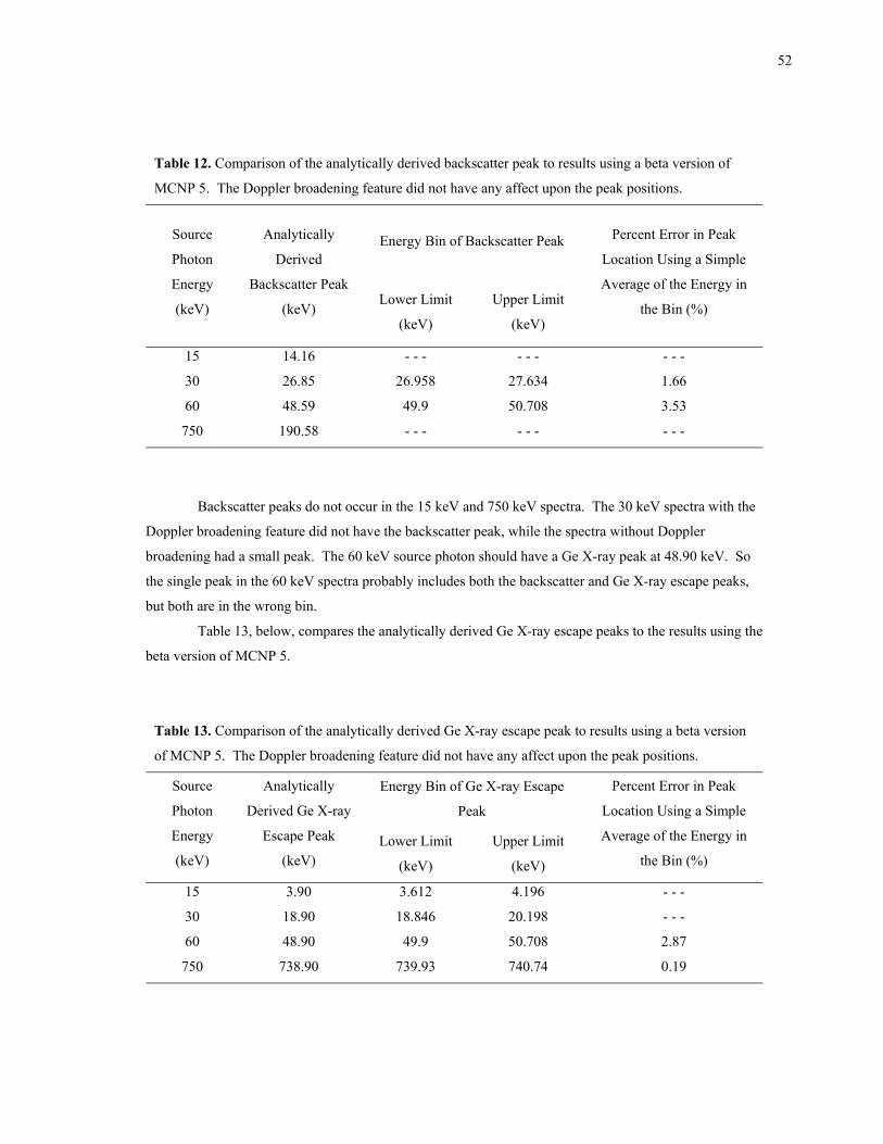
52
Table 12. Comparison of the analytically derived backscatter peak to results using a beta version of
MCNP 5. The Doppler broadening feature did not have any affect upon the peak positions.
Energy Bin of Backscatter Peak Source
Photon
Energy
(keV)
Analytically
Derived
Backscatter Peak
(keV) Lower Limit
(keV)
Upper Limit
(keV)
Percent Error in Peak
Location Using a Simple
Average of the Energy in
the Bin (%)
15 14.16 - - - - - - - - -
30 26.85 26.958 27.634 1.66
60 48.59 49.9 50.708 3.53
750 190.58 - - - - - - - - -
Backscatter peaks do not occur in the 15 keV and 750 keV spectra. The 30 keV spectra with the
Doppler broadening feature did not have the backscatter peak, while the spectra without Doppler
broadening had a small peak. The 60 keV source photon should have a Ge X-ray peak at 48.90 keV. So
the single peak in the 60 keV spectra probably includes both the backscatter and Ge X-ray escape peaks,
but both are in the wrong bin.
Table 13, below, compares the analytically derived Ge X-ray escape peaks to the results using the
beta version of MCNP 5.
Table 13. Comparison of the analytically derived Ge X-ray escape peak to results using a beta version
of MCNP 5. The Doppler broadening feature did not have any affect upon the peak positions.
Energy Bin of Ge X-ray Escape
Peak
Source
Photon
Energy
(keV)
Analytically
Derived Ge X-ray
Escape Peak
(keV) Lower Limit
(keV)
Upper Limit
(keV)
Percent Error in Peak
Location Using a Simple
Average of the Energy in
the Bin (%)
15 3.90 3.612 4.196 - - -
30 18.90 18.846 20.198 - - -
60 48.90 49.9 50.708 2.87
750 738.90 739.93 740.74 0.19
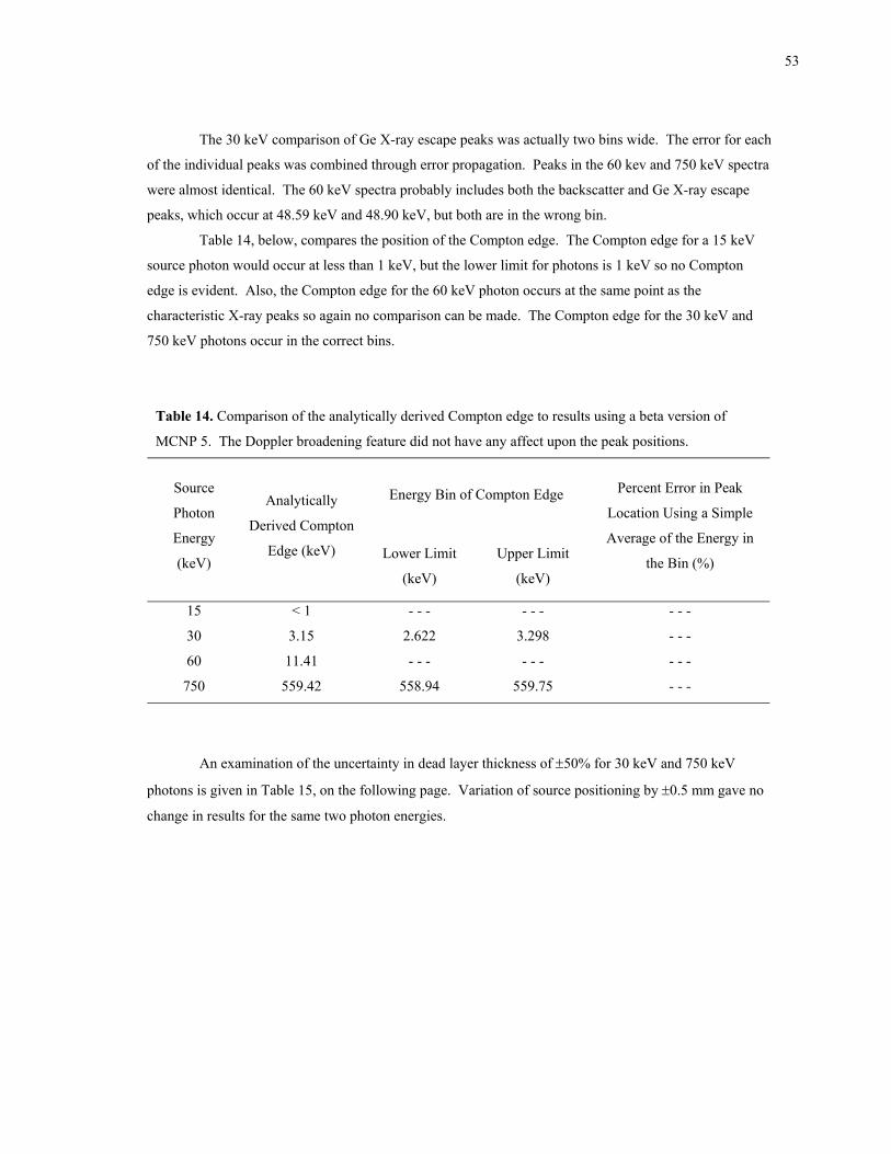
53
The 30 keV comparison of Ge X-ray escape peaks was actually two bins wide. The error for each
of the individual peaks was combined through error propagation. Peaks in the 60 kev and 750 keV spectra
were almost identical. The 60 keV spectra probably includes both the backscatter and Ge X-ray escape
peaks, which occur at 48.59 keV and 48.90 keV, but both are in the wrong bin.
Table 14, below, compares the position of the Compton edge. The Compton edge for a 15 keV
source photon would occur at less than 1 keV, but the lower limit for photons is 1 keV so no Compton
edge is evident. Also, the Compton edge for the 60 keV photon occurs at the same point as the
characteristic X-ray peaks so again no comparison can be made. The Compton edge for the 30 keV and
750 keV photons occur in the correct bins.
Table 14. Comparison of the analytically derived Compton edge to results using a beta version of
MCNP 5. The Doppler broadening feature did not have any affect upon the peak positions.
Energy Bin of Compton Edge Source
Photon
Energy
(keV)
Analytically
Derived Compton
Edge (keV) Lower Limit
(keV)
Upper Limit
(keV)
Percent Error in Peak
Location Using a Simple
Average of the Energy in
the Bin (%)
15 < 1 - - - - - - - - -
30 3.15 2.622 3.298 - - -
60 11.41 - - - - - - - - -
750 559.42 558.94 559.75 - - -
An examination of the uncertainty in dead layer thickness of ±50% for 30 keV and 750 keV
photons is given in Table 15, on the following page. Variation of source positioning by ±0.5 mm gave no
change in results for the same two photon energies.
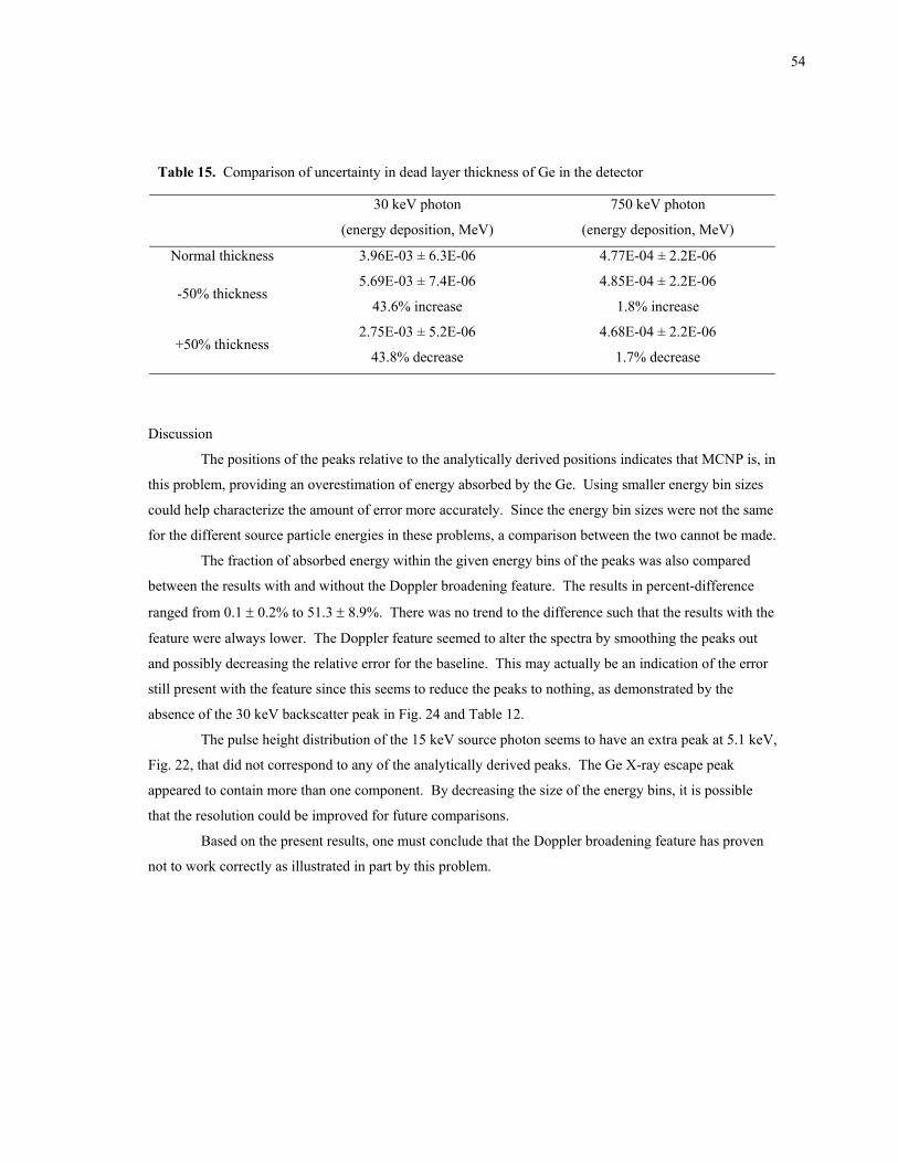
54
Table 15. Comparison of uncertainty in dead layer thickness of Ge in the detector
30 keV photon
(energy deposition, MeV)
750 keV photon
(energy deposition, MeV)
Normal thickness 3.96E-03 ± 6.3E-06 4.77E-04 ± 2.2E-06
5.69E-03 ± 7.4E-06 4.85E-04 ± 2.2E-06 -50% thickness
43.6% increase 1.8% increase
2.75E-03 ± 5.2E-06 4.68E-04 ± 2.2E-06 +50% thickness
43.8% decrease 1.7% decrease
Discussion
The positions of the peaks relative to the analytically derived positions indicates that MCNP is, in
this problem, providing an overestimation of energy absorbed by the Ge. Using smaller energy bin sizes
could help characterize the amount of error more accurately. Since the energy bin sizes were not the same
for the different source particle energies in these problems, a comparison between the two cannot be made.
The fraction of absorbed energy within the given energy bins of the peaks was also compared
between the results with and without the Doppler broadening feature. The results in percent-difference
ranged from 0.1 ± 0.2% to 51.3 ± 8.9%. There was no trend to the difference such that the results with the
feature were always lower. The Doppler feature seemed to alter the spectra by smoothing the peaks out
and possibly decreasing the relative error for the baseline. This may actually be an indication of the error
still present with the feature since this seems to reduce the peaks to nothing, as demonstrated by the
absence of the 30 keV backscatter peak in Fig. 24 and Table 12.
The pulse height distribution of the 15 keV source photon seems to have an extra peak at 5.1 keV,
Fig. 22, that did not correspond to any of the analytically derived peaks. The Ge X-ray escape peak
appeared to contain more than one component. By decreasing the size of the energy bins, it is possible
that the resolution could be improved for future comparisons.
Based on the present results, one must conclude that the Doppler broadening feature has proven
not to work correctly as illustrated in part by this problem.
55
CONCLUSION
Anisotropic and radial dose profiles were determined for a 192Ir brachytherapy device. The
anisotropic profile showed the greatest dose to be on the transverse axis, 90o relative to the axis of the
source and cable, with the smallest dose on the axis of the source and cable. A comparison was made
between the *F8 tally and the F6 tally. Results showed that for this problem, the results and standard
deviation for the *F8 tally were outside of the results and standard deviation of the F6 tally. Also, the
precision for the F6 tally was often smaller by half an order of magnitude than the *F8 tally.
A 32P source was used in the second brachytherapy device. The radial dose profile was
determined along with the dose rate 1 mm within the artery wall along the source longitudinal axis. This
problem was an excellent demonstration of what can happen when the source is biased, resulting in
erroneous results. With the source (over) biased, a drop in dose rate is present 1 mm within the artery wall
along the center of the source cylinder longitudinal axis. The magnitude of error also increased
significantly for the dose rate indicating the results were questionable. With no biasing, the dose rate
profile 1 mm within the artery wall along the source longitudinal axis proved to be an even distribution of
about 0.21 Gy s-1 for almost the entire length of the source cylinder.
Problem 4 was modeled to determine photon and neutron response for several different source
energies to a TLD upon an ISO slab phantom. This problem included a comparison of results of the
neutron physics with and without the S(α,β) cross sections. There was a significant difference between
the results. The largest percent-difference occurred with the highest energy neutrons, but this difference
had such a significant error that the results were not reliable. The use of the S(α,β) cross sections is
limited to neutrons and only a few materials. These cross sections may potentially have a great effect
upon the results of low energy photons. Hopefully, they will increase the accuracy of these results by
improving the low energy physics to include resonances in the cross sections that will take into account
molecular properties like bond vibrations and rotations.
When comparing MCNP versions 4C2 and 5beta3.23, with each run starting at the same random
number and tracking to end at 50 million histories, it was found that the tally results, slope, vov, error, nrn,
and collisions were identical. The only difference was the ctm, which ran 58% longer in version 5beta3.23
when compared to 4C2.
Air kerma backscatter profiles on the front face of an ISO slab phantom were determined along
the apothem and diagonal of the front face. The results determined with MCNP were compared to
experimental results found in ICRP 74 and give an indication of reasonable agreement between the two.
Since the Ka (free in air) obtained in this problem used a spectrum of source photons, a direct comparison
between ICRP 74, which used monoenergetic photons, was not considered practical.
56
Both the indirect spectral (angular distribution) and indirect energy fluence were determined for
two 12-inch diameter Bonner spheres located in a neutron detector calibration room in problem 6. The
indirect contribution was very small with the largest contribution coming from low energy photons at an
average polar angle of 47o relative to particles crossing a plane parallel to the floor.
The final problem looked at pulse height distribution spectra for a Ge detector. A comparison
was made of spectra with the new Doppler broadening feature to spectra without the feature. The peaks
within these spectra were also compared with analytically derived peaks for an indication of accuracy.
Spectra with the Doppler broadening feature compared very well with spectra without the feature
in terms of peak positions. The positions of the peaks relative to the analytically derived positions
indicates that MCNP, in this problem, provided an overestimation of energy absorbed by the Ge. Using
smaller energy bin sizes could help to better characterize an associated amount of error. The magnitude of
the tally results (peak sizes) with and without the Doppler broadening feature varied between 0.1 ± 0.2%
to 51.3 ± 8.9%. This will probably change when the feature, which is not working properly as shown in
part by this problem, is corrected.
57
REFERENCES
Amols HI. Intravascular brachytherapy physics: introduction. Proceeding of the 22nd Annual EMBS International Conference. Chicago: EMBS; 2000: 1573-1576.
Attix FH. Introduction to radiological physics and radiation dosimetry. New York: John Wiley & Sons; 1986.
Bast RC, Kufe DW, Pollock RE, Weichselbaum RR, Holland JF, Frei E, Gansler TS. Cancer Medicine. Available at: http://www.ncbi.nlm.nih.gov/books/bv.fcgi?call=bv.View..ShowTOC&rid=cmed.TOC&depth=2: BC Decker Inc.; 2000. Accessed 22 January 2003.
Briesmeister JF. MCNP – a general monte carlo n-particle transport code, version 4C. Los Alamos: LA-13709-M; 2000.
Brown FB. MCNP version 5. ANS Winter Meeting. Washington D.C. 2002.
Gualdrini G. personal communication, QUADOS a concerted action of the European Commission. 30 January 2003.
Knoll GF. Radiation detection and measurement. New York: John Wiley & Sons; 2000.
Price R. 32P Beta Spectrum. Available at: http://members.aol.com/rprice1495/data/P32. Accessed 1 June 2002.
Selcow EC, Goorley JT. Medical physics application of MCNP. Radiation Protection & Shielding Division of the American Nuclear Society, 12th Biennial RPSD Topical Meeting; Los Alamos: LA-UR-02-2043; 2002.
Siebert B. Intercomparison on the Usage of Computational Code in Radiation Dosimetry. Available at: http://www.nea.fr/download/quados/quados.html. Accessed 22 January 2003.
Sood A. Doppler energy broadening for incoherent scattering in MCNP, Part I. Los Alamos: X5:AS-02-16; 2002.
WebElements.com [online]. Available at: http://www.webelements.com/. Accessed 22 January 2003.
Wong T, Wallace S, Fernando W, Schumer W, Quong G. Dose errors in the near field of an HDR brachytherapy stepping source. Phys. Med. Biol. 44:357-363; 1999.
58
APPENDIX A
Problem 1, 192Ir Brachytherapy Source Message: outp=p1o.o runtpe=p1r.r mctal=p1m.m Ir-192 Brachytherapy source c Beginning of Cell Cards c c source 1 2 -22.42 (-11 21 -23): (-20 -21): (-22 23) imp:p,e 1 c steel capsule 4 1 -8.02 -10 11 -1 25 imp:p,e 1 $ radius of capsule; 0.0325 to 0.045 5 1 -8.02 -24 -25 -10 imp:p,e 1 $ cap of capsule 6 1 -8.02 20 -21 25 -11 imp:p,e 1 $ space outside source cap on left 7 1 -8.02 -1 23 22 -11 imp:p,e 1 $ space outside source cap on right 8 1 -8.02 1 -2 -300 imp:p,e 1 $ inside of the cone; other cap c c woven steel cable 9 4 -4.81 2 -150 -12 imp:p,e 1 $ woven steel cable c with radius 0.035 c c axial fill material c 10 3 -1.0 -10 12 -150 1 235 c 11 3 -1.0 1 300 -150 12 -10 235 c c Dose Depth Cells c radial depth by cylinders c 15 3 -1.0 10 -100 -150 $ outside of the steel capsule c to 1 cm radius cylinder c 16 3 -1.0 100 -101 -150 $ 1 - 2 cm radius depth c 17 3 -1.0 101 -102 -150 $ 2 - 3 cm radius depth c 18 3 -1.0 102 -103 -150 $ 3 - 4 cm radius depth c 19 3 -1.0 103 -104 -150 $ 4 - 5 cm radius depth c c wedges of a sphere centered at the origin with a radius of 5 cm 20 3 -1.0 -150 235 201 10 imp:p,e 1 $ 0 to 10 22 3 -1.0 -150 235 -201 203 10 imp:p,e 1 $ 10 to 20 24 3 -1.0 -150 -203 205 235 10 imp:p,e 1 $ 20 to 30 26 3 -1.0 -150 -205 207 235 10 imp:p,e 1 $ 30 to 40 28 3 -1.0 -150 -207 209 235 10 imp:p,e 1 $ 40 to 50 30 3 -1.0 -150 -209 211 235 10 imp:p,e 1 $ 50 to 60 32 3 -1.0 -150 -211 213 235 10 imp:p,e 1 $ 60 to 70 34 3 -1.0 -150 -213 215 235 10 imp:p,e 1 $ 70 to 80 36 3 -1.0 -150 -215 217 235 10 imp:p,e 1 $ 80 to 90 38 3 -1.0 -150 -217 -219 235 10 imp:p,e 1 $ 90 to 100 40 3 -1.0 -150 219 -221 235 10 imp:p,e 1 $ 100 to 110 42 3 -1.0 -150 221 -223 235 10 imp:p,e 1 $ 110 to 120 44 3 -1.0 -150 223 -225 235 10 imp:p,e 1 $ 120 to 130 46 3 -1.0 -150 225 -227 235 10 imp:p,e 1 $ 130 to 140
59
48 3 -1.0 -150 227 -229 235 10 imp:p,e 1 $ 140 to 150 50 3 -1.0 -150 229 -231 235 10 imp:p,e 1 $ 150 to 160 52 3 -1.0 -150 231 -233 235 10 imp:p,e 1 $ 160 to 170 54 3 -1.0 -150 233 235 10 imp:p,e 1 $ 170 to 180 c c fill cells 70 3 -1.0 (24 -10 -25 -150):(1 300 -2 -10 -150):(2 12 -10 -150) imp:p,e 1 71 3 -1.0 -150 -235 10 imp:p,e 1 c c outside the known universe 99 0 150 imp:p,e 0 $ outside of the problem c c End of Cell Cards c Beginning of Surface Cards c 1 px 0.235 $ larger end of cone 2 px 0.25 $ smaller end of cone c 3 px -0.2 $ end of catheter c 10 cx 0.045 $ outside radius of steel capsule 11 cx 0.0325 $ inside radius of steel capsule; max radius of Ir-192 12 cx 0.035 $ radius of woven steel cable c 20 sx -0.1475 0.0325 $ sphere approximating Ir-192 core cap 21 px -0.1475 $ plane cuting sphere to approximate Ir-192 core cap 22 sx 0.1475 0.0325 $ sphere approximating Ir-192 core cap 23 px 0.1475 $ plane cuting sphere to approximate Ir-192 core cap c 24 sx -0.139 0.061 $ sphere approximating end of steel encapsulation 25 px -0.18 $ plane cutting the sphere in half c c 100 cx 1 c 101 cx 2 c 102 cx 3 c 103 cx 4 c 104 cx 5 c c 125 so 0.201 $ outside of device except cable 150 so 5 $ boundary of problem c c 200 p 0.08748866 -1 0 0 $ 5 degrees 201 p 0.176327 -1 0 0 $ 10 degrees c 202 p 0.267949 -1 0 0 $ 15 degrees 203 p 0.36397 -1 0 0 $ 20 degrees c 204 p 0.4663 -1 0 0 $ 25 degrees 205 p 0.57735 -1 0 0 $ 30 degrees c 206 p 0.7002 -1 0 0 $ 35 degrees 207 p 0.8391 -1 0 0 $ 40 degrees c 208 p 1 -1 0 0 $ 45 degrees 209 p 1.19175 -1 0 0 $ 50 degrees c 210 p 1.428148 -1 0 0 $ 55 degrees
60
211 p 1.732 -1 0 0 $ 60 degrees c 212 p 2.1445 -1 0 0 $ 65 degrees 213 p 2.7475 -1 0 0 $ 70 degrees c 214 p 3.73205 -1 0 0 $ 75 degrees 215 p 5.67128 -1 0 0 $ 80 degrees c 216 p 11.43 -1 0 0 $ 85 degrees 217 px 0 $ 90 degrees c 218 p -11.43 -1 0 0 $ 95 degrees 219 p -5.67128 -1 0 0 $ 100 degrees c 220 p -3.73205 -1 0 0 $ 105 degrees 221 p -2.7475 -1 0 0 $ 110 degrees c 222 p -2.1445 -1 0 0 $ 115 degrees 223 p -1.732 -1 0 0 $ 120 degrees c 224 p -1.428148 -1 0 0 $ 125 degrees 225 p -1.19175 -1 0 0 $ 130 degrees c 226 p -1 -1 0 0 $ 135 degrees 227 p -0.8391 -1 0 0 $ 140 degrees c 228 p -0.7002 -1 0 0 $ 145 degrees 229 p -0.57735 -1 0 0 $ 150 degrees c 230 p -0.4663 -1 0 0 $ 155 degrees 231 p -0.36397 -1 0 0 $ 160 degrees c 232 p -0.267949 -1 0 0 $ 165 degrees 233 p -0.176327 -1 0 0 $ 170 degrees c 234 p -0.08748866 -1 0 0 $ 175 degrees 235 py 0 $ 0 or 180 degrees c c Cone joining the steel encapsulation with the woven steel cable 300 kx 0.3025 0.444444 -1 $ -1 indicates cone opens in - dir c c End of Surface Cards c Beginning of Data Cards c mode P c print c prdmp 2j 1 c nps 110000000 c c input volume for tallying wedges vol 7j 14.512589 14.544398 15r 14.512589 3j c c Source Definition c Isotropic cylindrical volume source sdef pos=0 0 0 cel 1 axs=1 0 0 rad=d1 ext=d2 erg=d3 par 2 si1 0.0325 sp1 -21 1 c sb1 -21 4 si2 0.18 c sp2 -21 0 c sb2 -21 1 c These energies (MeV) and probabilities (normalized) are for the
61
c photons after electron emission c http://members.aol.com/rprice1495/data/Ir192.pdf si3 0 0.06149 0.06300 0.07130 0.07340 0.11009 0.13634 0.17698 0.20131 0.20580 0.28004 0.28327 0.29596 0.30847 0.31651 0.32931 0.37449 0.41647 0.42053 0.46807 0.48458 0.48530 0.48904 0.58859 0.59337 0.59940 0.60442 0.61247 0.70398 0.76600 0.88454 1.06148 1.08970 1.37830 c sp3 0 0.00713192 0.00904863 0.00295484 0.000772031 0.0000565651 0.000818388 0.0000191136 0.00210347 0.0147230 0.000103680 0.00117097 0.0127795 0.0145714 0.369344 0.0000827303 0.00321293 0.00296153 0.000327088 0.213200 0.0142059 0.00000980639 0.00197599 0.0201254 0.000189531 0.0000172860 0.0366937 0.0236646 0.0000238206 0.00000665052 0.00130113 0.000235353 0.00000478285 0.00000553616 c c Cell Importances c c imp:e 1 46r 1 0 c imp:p 1 46r 1 0 c c Tallies c c Point detectors will give MeV/cm^2 c de and df card info from Attix, mass energy-absorption coefficient c c f5:p 1 0 0 0 $ 1 cm from 0,0,0 - 0 degrees c c f15:p 0.984808 0.173648 0 0 $ 1 cm from 0,0,0 - 10 degrees c c f25:p 0.939693 0.342020 0 0 $ 1 cm from 0,0,0 - 20 degrees c c f35:p 0.866025 0.5 0 0 $ 1 cm from 0,0,0 - 30 degrees c c f45:p 0.766044 0.642788 0 0 $ 1 cm from 0,0,0 - 40 degrees c c f55:p 0.642788 0.766044 0 0 $ 1 cm from 0,0,0 - 50 degrees c c f65:p 0.5 0.866025 0 0 $ 1 cm from 0,0,0 - 60 degrees c de65 0.0100 0.015 0.02 0.03 0.04 0.05 0.06 0.08 0.1 c 0.15 0.2 0.3 0.4 0.5 0.6 0.8 1.0 1.5 2.0000 c df65 4.79 1.28 0.512 0.149 0.0677 0.0418 0.0320 c 0.0262 0.0256 0.0277 0.0297 0.0319 0.0328 c 0.0330 0.0329 0.0321 0.0309 0.0282 0.0260 c f75:p 0.342020 0.939693 0 0 $ 1 cm from 0,0,0 - 70 degrees c f85:p 0.173648 0.984808 0 0 $ 1 cm from 0,0,0 - 80 degrees c f95:p 0 1 0 0 $ 1 cm from 0,0,0 - 90 degrees c de95 0.0100 0.015 0.02 0.03 0.04 0.05 0.06 0.08 0.1 c 0.15 0.2 0.3 0.4 0.5 0.6 0.8 1.0 1.5 2.0000 c df95 4.79 1.28 0.512 0.149 0.0677 0.0418 0.0320 c 0.0262 0.0256 0.0277 0.0297 0.0319 0.0328 c 0.0330 0.0329 0.0321 0.0309 0.0282 0.0260 c f105:p -0.173648 0.984808 0 0 $ 1 cm from 0,0,0 - 100 degrees
62
c f115:p -0.342020 0.939693 0 0 $ 1 cm from 0,0,0 - 110 degrees c f125:p -0.5 0.866025 0 0 $ 1 cm from 0,0,0 - 120 degrees c f135:p -0.642788 0.766044 0 0 $ 1 cm from 0,0,0 - 130 degrees c de135 0.0100 0.015 0.02 0.03 0.04 0.05 0.06 0.08 0.1 c 0.15 0.2 0.3 0.4 0.5 0.6 0.8 1.0 1.5 2.0000 c df135 4.79 1.28 0.512 0.149 0.0677 0.0418 0.0320 c 0.0262 0.0256 0.0277 0.0297 0.0319 0.0328 c 0.0330 0.0329 0.0321 0.0309 0.0282 0.0260 c f145:p -0.766044 0.642788 0 0 $ 1 cm from 0,0,0 - 140 degrees c f155:p -0.866025 0.5 0 0 $ 1 cm from 0,0,0 - 150 degrees c f165:p -0.939693 0.342020 0 0 $ 1 cm from 0,0,0 - 160 degrees c f175:p -0.984808 0.173648 0 0 $ 1 cm from 0,0,0 - 170 degrees c f185:p -1 0 0 0 $ 1 cm from 0,0,0 - 180 degrees c fc6 Energy deposition (MeV/g) per source photon) f6 tallies are the anisotropic dose determination f6:p 20 22 fm6 1.602e-10 $ convert MeV/g to Gy f16:p 24 26 28 30 32 34 36 38 40 42 44 46 48 50 fm16 1.602e-10 f26:p 52 54 fm26 1.602e-10 c fc8 Total energy deposition (MeV) in each of the f8 tallies are the anisotropic dose determination *f8:p 20 22 *f18:p 24 26 28 30 32 34 36 38 40 42 44 46 48 50 *f28:p 52 54 c c Beginning of Material Data Cards c c AISI Type 316L -- Stainless Steel c rho = 8.02 g/cc m1 025000 -0.02 014000 -0.01 024000 -0.17 028000 -0.12 026000 -0.68 c c Ir-192 pure cylindrical source c rho = 22.42 g/cc m2 077192 1 c c Homogenous Liquid Water c rho = 1.0 g/cc m3 001000 1 008000 2 c c Woven Steel Cable (assumed to be same steel as capsule) c rho = 4.81 g/cc m4 025000 -0.02 014000 -0.01 024000 -0.17
028000 -0.12 026000 -0.68
63
Problem 2, 32P Brachytherapy Source Message: outp=p1o.o runtpe=p1r.r mctal=p1m.m Ir-192 Brachytherapy source c Beginning of Cell Cards c c source 1 2 -22.42 (-11 21 -23): (-20 -21): (-22 23) imp:p,e 1 c steel capsule 4 1 -8.02 -10 11 -1 25 imp:p,e 1 $ radius of capsule; 0.0325 to 0.045 5 1 -8.02 -24 -25 -10 imp:p,e 1 $ cap of capsule 6 1 -8.02 20 -21 25 -11 imp:p,e 1 $ space outside source cap on left 7 1 -8.02 -1 23 22 -11 imp:p,e 1 $ space outside source cap on right 8 1 -8.02 1 -2 -300 imp:p,e 1 $ inside of the cone; other cap c c woven steel cable 9 4 -4.81 2 -150 -12 imp:p,e 1 $ woven steel cable c with radius 0.035 c c axial fill material c 10 3 -1.0 -10 12 -150 1 235 c 11 3 -1.0 1 300 -150 12 -10 235 c c Dose Depth Cells c radial depth by cylinders c 15 3 -1.0 10 -100 -150 $ outside of the steel capsule c to 1 cm radius cylinder c 16 3 -1.0 100 -101 -150 $ 1 - 2 cm radius depth c 17 3 -1.0 101 -102 -150 $ 2 - 3 cm radius depth c 18 3 -1.0 102 -103 -150 $ 3 - 4 cm radius depth c 19 3 -1.0 103 -104 -150 $ 4 - 5 cm radius depth c c wedges of a sphere centered at the origin with a radius of 5 cm 20 3 -1.0 -150 235 201 10 imp:p,e 1 $ 0 to 10 22 3 -1.0 -150 235 -201 203 10 imp:p,e 1 $ 10 to 20 24 3 -1.0 -150 -203 205 235 10 imp:p,e 1 $ 20 to 30 26 3 -1.0 -150 -205 207 235 10 imp:p,e 1 $ 30 to 40 28 3 -1.0 -150 -207 209 235 10 imp:p,e 1 $ 40 to 50 30 3 -1.0 -150 -209 211 235 10 imp:p,e 1 $ 50 to 60 32 3 -1.0 -150 -211 213 235 10 imp:p,e 1 $ 60 to 70 34 3 -1.0 -150 -213 215 235 10 imp:p,e 1 $ 70 to 80 36 3 -1.0 -150 -215 217 235 10 imp:p,e 1 $ 80 to 90 38 3 -1.0 -150 -217 -219 235 10 imp:p,e 1 $ 90 to 100 40 3 -1.0 -150 219 -221 235 10 imp:p,e 1 $ 100 to 110 42 3 -1.0 -150 221 -223 235 10 imp:p,e 1 $ 110 to 120 44 3 -1.0 -150 223 -225 235 10 imp:p,e 1 $ 120 to 130 46 3 -1.0 -150 225 -227 235 10 imp:p,e 1 $ 130 to 140 48 3 -1.0 -150 227 -229 235 10 imp:p,e 1 $ 140 to 150 50 3 -1.0 -150 229 -231 235 10 imp:p,e 1 $ 150 to 160 52 3 -1.0 -150 231 -233 235 10 imp:p,e 1 $ 160 to 170
64
54 3 -1.0 -150 233 235 10 imp:p,e 1 $ 170 to 180 c c fill cells 70 3 -1.0 (24 -10 -25 -150):(1 300 -2 -10 -150):(2 12 -10 -150) imp:p,e 1 71 3 -1.0 -150 -235 10 imp:p,e 1 c c outside the known universe 99 0 150 imp:p,e 0 $ outside of the problem c c End of Cell Cards c Beginning of Surface Cards c 1 px 0.235 $ larger end of cone 2 px 0.25 $ smaller end of cone c 3 px -0.2 $ end of catheter c 10 cx 0.045 $ outside radius of steel capsule 11 cx 0.0325 $ inside radius of steel capsule; max radius of Ir-192 12 cx 0.035 $ radius of woven steel cable c 20 sx -0.1475 0.0325 $ sphere approximating Ir-192 core cap 21 px -0.1475 $ plane cuting sphere to approximate Ir-192 core cap 22 sx 0.1475 0.0325 $ sphere approximating Ir-192 core cap 23 px 0.1475 $ plane cuting sphere to approximate Ir-192 core cap c 24 sx -0.139 0.061 $ sphere approximating end of steel encapsulation 25 px -0.18 $ plane cutting the sphere in half c c 100 cx 1 c 101 cx 2 c 102 cx 3 c 103 cx 4 c 104 cx 5 c c 125 so 0.201 $ outside of device except cable 150 so 5 $ boundary of problem c c 200 p 0.08748866 -1 0 0 $ 5 degrees 201 p 0.176327 -1 0 0 $ 10 degrees c 202 p 0.267949 -1 0 0 $ 15 degrees 203 p 0.36397 -1 0 0 $ 20 degrees c 204 p 0.4663 -1 0 0 $ 25 degrees 205 p 0.57735 -1 0 0 $ 30 degrees c 206 p 0.7002 -1 0 0 $ 35 degrees 207 p 0.8391 -1 0 0 $ 40 degrees c 208 p 1 -1 0 0 $ 45 degrees 209 p 1.19175 -1 0 0 $ 50 degrees c 210 p 1.428148 -1 0 0 $ 55 degrees 211 p 1.732 -1 0 0 $ 60 degrees c 212 p 2.1445 -1 0 0 $ 65 degrees 213 p 2.7475 -1 0 0 $ 70 degrees
65
c 214 p 3.73205 -1 0 0 $ 75 degrees 215 p 5.67128 -1 0 0 $ 80 degrees c 216 p 11.43 -1 0 0 $ 85 degrees 217 px 0 $ 90 degrees c 218 p -11.43 -1 0 0 $ 95 degrees 219 p -5.67128 -1 0 0 $ 100 degrees c 220 p -3.73205 -1 0 0 $ 105 degrees 221 p -2.7475 -1 0 0 $ 110 degrees c 222 p -2.1445 -1 0 0 $ 115 degrees 223 p -1.732 -1 0 0 $ 120 degrees c 224 p -1.428148 -1 0 0 $ 125 degrees 225 p -1.19175 -1 0 0 $ 130 degrees c 226 p -1 -1 0 0 $ 135 degrees 227 p -0.8391 -1 0 0 $ 140 degrees c 228 p -0.7002 -1 0 0 $ 145 degrees 229 p -0.57735 -1 0 0 $ 150 degrees c 230 p -0.4663 -1 0 0 $ 155 degrees 231 p -0.36397 -1 0 0 $ 160 degrees c 232 p -0.267949 -1 0 0 $ 165 degrees 233 p -0.176327 -1 0 0 $ 170 degrees c 234 p -0.08748866 -1 0 0 $ 175 degrees 235 py 0 $ 0 or 180 degrees c c Cone joining the steel encapsulation with the woven steel cable 300 kx 0.3025 0.444444 -1 $ -1 indicates cone opens in - dir c c End of Surface Cards c Beginning of Data Cards c mode P c print c prdmp 2j 1 c nps 110000000 c c input volume for tallying wedges vol 7j 14.512589 14.544398 15r 14.512589 3j c c Source Definition c Isotropic cylindrical volume source sdef pos=0 0 0 cel 1 axs=1 0 0 rad=d1 ext=d2 erg=d3 par 2 si1 0.0325 sp1 -21 1 c sb1 -21 4 si2 0.18 c sp2 -21 0 c sb2 -21 1 c These energies (MeV) and probabilities (normalized) are for the c photons after electron emission c http://members.aol.com/rprice1495/data/Ir192.pdf si3 0 0.06149 0.06300 0.07130 0.07340 0.11009 0.13634 0.17698
66
0.20131 0.20580 0.28004 0.28327 0.29596 0.30847 0.31651 0.32931 0.37449 0.41647 0.42053 0.46807 0.48458 0.48530 0.48904 0.58859 0.59337 0.59940 0.60442 0.61247 0.70398 0.76600 0.88454 1.06148 1.08970 1.37830 c sp3 0 0.00713192 0.00904863 0.00295484 0.000772031 0.0000565651 0.000818388 0.0000191136 0.00210347 0.0147230 0.000103680 0.00117097 0.0127795 0.0145714 0.369344 0.0000827303 0.00321293 0.00296153 0.000327088 0.213200 0.0142059 0.00000980639 0.00197599 0.0201254 0.000189531 0.0000172860 0.0366937 0.0236646 0.0000238206 0.00000665052 0.00130113 0.000235353 0.00000478285 0.00000553616 c c Cell Importances c c imp:e 1 46r 1 0 c imp:p 1 46r 1 0 c c Tallies c c Point detectors will give MeV/cm^2 c de and df card info from Attix, mass energy-absorption coefficient c c f5:p 1 0 0 0 $ 1 cm from 0,0,0 - 0 degrees c c f15:p 0.984808 0.173648 0 0 $ 1 cm from 0,0,0 - 10 degrees c c f25:p 0.939693 0.342020 0 0 $ 1 cm from 0,0,0 - 20 degrees c c f35:p 0.866025 0.5 0 0 $ 1 cm from 0,0,0 - 30 degrees c c f45:p 0.766044 0.642788 0 0 $ 1 cm from 0,0,0 - 40 degrees c c f55:p 0.642788 0.766044 0 0 $ 1 cm from 0,0,0 - 50 degrees c c f65:p 0.5 0.866025 0 0 $ 1 cm from 0,0,0 - 60 degrees c de65 0.0100 0.015 0.02 0.03 0.04 0.05 0.06 0.08 0.1 c 0.15 0.2 0.3 0.4 0.5 0.6 0.8 1.0 1.5 2.0000 c df65 4.79 1.28 0.512 0.149 0.0677 0.0418 0.0320 c 0.0262 0.0256 0.0277 0.0297 0.0319 0.0328 c 0.0330 0.0329 0.0321 0.0309 0.0282 0.0260 c f75:p 0.342020 0.939693 0 0 $ 1 cm from 0,0,0 - 70 degrees c f85:p 0.173648 0.984808 0 0 $ 1 cm from 0,0,0 - 80 degrees c f95:p 0 1 0 0 $ 1 cm from 0,0,0 - 90 degrees c de95 0.0100 0.015 0.02 0.03 0.04 0.05 0.06 0.08 0.1 c 0.15 0.2 0.3 0.4 0.5 0.6 0.8 1.0 1.5 2.0000 c df95 4.79 1.28 0.512 0.149 0.0677 0.0418 0.0320 c 0.0262 0.0256 0.0277 0.0297 0.0319 0.0328 c 0.0330 0.0329 0.0321 0.0309 0.0282 0.0260 c f105:p -0.173648 0.984808 0 0 $ 1 cm from 0,0,0 - 100 degrees c f115:p -0.342020 0.939693 0 0 $ 1 cm from 0,0,0 - 110 degrees c f125:p -0.5 0.866025 0 0 $ 1 cm from 0,0,0 - 120 degrees c f135:p -0.642788 0.766044 0 0 $ 1 cm from 0,0,0 - 130 degrees
67
c de135 0.0100 0.015 0.02 0.03 0.04 0.05 0.06 0.08 0.1 c 0.15 0.2 0.3 0.4 0.5 0.6 0.8 1.0 1.5 2.0000 c df135 4.79 1.28 0.512 0.149 0.0677 0.0418 0.0320 c 0.0262 0.0256 0.0277 0.0297 0.0319 0.0328 c 0.0330 0.0329 0.0321 0.0309 0.0282 0.0260 c f145:p -0.766044 0.642788 0 0 $ 1 cm from 0,0,0 - 140 degrees c f155:p -0.866025 0.5 0 0 $ 1 cm from 0,0,0 - 150 degrees c f165:p -0.939693 0.342020 0 0 $ 1 cm from 0,0,0 - 160 degrees c f175:p -0.984808 0.173648 0 0 $ 1 cm from 0,0,0 - 170 degrees c f185:p -1 0 0 0 $ 1 cm from 0,0,0 - 180 degrees c fc6 Energy deposition (MeV/g) per source photon) f6 tallies are the anisotropic dose determination f6:p 20 22 fm6 1.602e-10 $ convert MeV/g to Gy f16:p 24 26 28 30 32 34 36 38 40 42 44 46 48 50 fm16 1.602e-10 f26:p 52 54 fm26 1.602e-10 c fc8 Total energy deposition (MeV) in each of the f8 tallies are the anisotropic dose determination *f8:p 20 22 *f18:p 24 26 28 30 32 34 36 38 40 42 44 46 48 50 *f28:p 52 54 c c Beginning of Material Data Cards c c AISI Type 316L -- Stainless Steel c rho = 8.02 g/cc m1 025000 -0.02 014000 -0.01 024000 -0.17 028000 -0.12 026000 -0.68 c c Ir-192 pure cylindrical source c rho = 22.42 g/cc m2 077192 1 c c Homogenous Liquid Water c rho = 1.0 g/cc m3 001000 1 008000 2 c c Woven Steel Cable (assumed to be same steel as capsule) c rho = 4.81 g/cc m4 025000 -0.02 014000 -0.01 024000 -0.17 028000 -0.12 026000 -0.68
68
Problem 4, Neutron and Photon Response of a TLD-Albedo Personal Dosemeter on an ISO Slab Phantom Message: outp=p4nt.o runtpe=p4nt.r mctal=p4nt.m wwout=wwout Neutron and Photon TLD Response on an ISO slab phantom c Beginning of Cell Cards c c TLDs 1 4 -2.54 5 -6 23 -24 37 -38 imp:n 7 $ Li-6F; chip 1; top left 2 5 -2.64 7 -8 23 -24 37 -38 imp:n 7 $ Li-7F; chip 2; top right 3 4 -2.54 5 -6 19 -20 37 -38 imp:n 7 $ Li-6F; chip 3; bottom left 4 5 -2.64 7 -8 19 -20 37 -38 imp:n 7 $ Li-7F; chip 4; bottom right c c water phantom c Cell 10 is the PMMA cube 10 1 -1.19 (1 -2 15 -28 40 -42):(11 -12 15 -28 40 -42) :(15 -16 1 -12 40 -42):(27 -28 1 -12 40 -42) :(39 -40 1 -12 15 -28):(41 -42 1 -12 15 -28) imp:n 1 11 3 -1.00 2 -11 16 -27 40 -41 imp:n 1 $ water inside ISO phantom c c Al plate 20 2 -2.70 (4 -9 18 -19 37 -38):(4 -9 24 -25 37 -38) :(4 -5 18 -25 37 -38):(8 -9 18 -25 37 -38) :(6 -7 18 -25 37 -38):(20 -23 4 -9 37 -38) imp:n 5 c c Al disks 25 2 -2.70 -52 36 -37 imp:n 30 $ in front of chip 3 26 2 -2.70 -53 36 -37 imp:n 30 $ in front of chip 4 c c vacuum disks 30 0 -52 38 -39 imp:n 7 $ behind chip 3 31 0 -53 38 -39 imp:n 7 $ behind chip 4 c c holder 35 6 -1.19 3 -10 38 -39 52 53 17 -26 imp:n 9 $ back with holes 36 6 -1.19 (3 -4 17 -26 37 -38):(9 -10 17 -26 37 -38) :(3 -10 25 -26 37 -38):(3 -10 17 -18 37 -38) imp:n 10 37 6 -1.19 3 -10 17 -26 36 -37 50 51 52 53 imp:n 9 38 6 -1.19 3 -10 17 -26 35 -36 50 51 imp:n 7 c c source 50 0 1 -12 15 -28 100 -101 imp:n 1 c c outside of problem 99 0 (-50 -37 101 -200):(-51 -37 101 -200):(-35 3 -10 17 -26 101 -200): (-3 -39 101 -200):(10 -39 101 -200):(-17 -39 101 -200): (26 -39 101 -200):((42:-1:12:-15:28:-100) -200) imp:n 2 999 0 200 imp:n 0 c c End of Cell Cards c Beginning of Surface Cards c
69
1 px -15 $ edge of water phantom; edge of PMMA 2 px -14 $ edge of PMMA; edge of water 3 px -1.75 $ edge of TLD; edge of polyethylene 4 px -1.25 $ edge of polyethylene; edge of Al 5 px -0.91 $ left edge of chips 1 and 3 6 px -0.59 $ right edge of chips 1 and 3 7 px 0.59 $ left edge of chips 2 and 4 8 px 0.91 $ right edge of chips 2 and 4 9 px 1.25 $ edge of Al; edge of polyethylene 10 px 1.75 $ edge of polyethylene; edge of TLD 11 px 14 $ edge of water; edge of PMMA 12 px 15 $ edge of PMMA; edge of water phantom c 15 py -15 $ edge of water phantom; edge of PMMA 16 py -14 $ edge of PMMA; edge of water 17 py -2.75 $ edge of TLD; edge of polyethylene 18 py -2.25 $ edge of polyethylene; edge of Al 19 py -1.91 $ edge of Al; bottom edge of chips 3 and 4 20 py -1.59 $ top edge of chips 3 and 4; edge of Al c 21 py -1.25 $ edge of Al c 22 py 1.25 $ edge of Al 23 py 1.59 $ edge of Al; bottom edge of chips 1 and 2 24 py 1.91 $ top edge of chips 1 and 2; edge of Al 25 py 2.25 $ edge of Al; edge of polyethylene 26 py 2.75 $ edge of polyethylene; edge of TLD 27 py 14 $ edge of water; edge of PMMA 28 py 15 $ edge of PMMA; edge of water phantom c 35 pz -0.79 $ front edge of TLD; edge of polyethylene 36 pz -0.39 $ edge of polyethylene; edge of Al disk 37 pz -0.29 $ edge of Al disk; front edge LiF 38 pz -0.20 $ edge of LiF; edge of vacuum or polyethylene 39 pz 0 $ back edge of TLD; edge of water phantom 40 pz 0.25 $ edge of PMMA; edge of water 41 pz 14 $ edge of water; edge of PMMA 42 pz 15 $ edge of PMMA; back edge of water phantom c 50 c/z -0.75 1.75 0.5 $ 1cm diameter hole centered on chip 1 51 c/z 0.75 1.75 0.5 $ 1cm diameter hole centered on chip 2 52 c/z -0.75 -1.75 0.5 $ 1cm diameter hole centered on chip 3 53 c/z 0.75 -1.75 0.5 $ 1cm diameter hole centered on chip 4 c c source providing neutrons and photons at normal incidence 100 pz -11 101 pz -10 c c surfaces to define the outside universe 200 so 30 c c End of Surface Cards c Beginning of Data Cards c
70
mode n c print c prdmp 2j 1 c c ctme 180 nps 200000000 c phys:p 100 0 0 c phys:e 50 0 0 0 0 0 c c Source Definition c Plane source with direction normal to surface sdef x=d1 y=d2 z=-10 sur=101 nrm=1 vec=0 0 -1 dir=-1 erg=0.0000000253 par 1 si1 -15 -2 2 15 sp1 0 1 1 1 sb1 0 1 20 1 si2 -15 -2.75 -0.5 0.5 2.75 15 sp2 0 1 1 1 1 1 sb2 0 1 20 1 20 1 c c Cell importances c c imp:e 1 15r 1 0 c imp:p 1 15r 1 0 c c Weight Window Generator wwp:n 10 1.1 5 0 -1 c wwg 14 0 0 mesh geom=xyz ref=0 0 0 origin= -30 -30 -30 imesh -2.0 2 30 iints 4 10 4 jmesh -7 -3 3 7 30 jints 4 10 15 10 4 kmesh -2 4 13 30 kints 4 10 7 4 c Tallies c c fc6 Energy deposition (MeV/g) per source photon) c f6 tallies are the cylindrical/radial dose depth c f6:p 1 2 3 4 T c fc4 n,t reactions in Li f4:n 1 3 $ Li-6 TLDs fm4 (1.4534e24 7 105) (1.4534e24 7 105) f14:n 2 4 $ Li-7 TLDs fm14 (9.0589e20 8 105) (9.0589e20 8 105) c c Beginning of Material Data Cards c c PMMA c rho = 1.19 g/cc m1 001001 -0.0805259 001002 -0.0000120807 $ naturally occurring H 008016 -0.319490706637 008017 -0.00012169590664 $nat. O 006012 -0.593190 006013 -0.00665831 $ naturally occurring C c c Aluminum
71
c rho = 2.70 g/cc m2 013027 1 c c Water c rho = 1.00 g/cc m3 001001 -0.111877 001002 -0.0000167841 $ naturally occurring H 008016 -0.88776398262 008017 -0.0003381549598 $ nat. O c c Li-6F c rho = 2.54 g/cc m4 003006 -0.229 003007 -0.012 009019 -0.758 c c Li-7F c rho = 2.64 g/cc m5 003006 -0.00016 003007 -0.270 009019 -0.730 c c Holder c rho = 1.19 g/cc m6 001001 -0.079988 001002 -0.000012 $ naturally occurring H 006012 -0.6279515 006013 -0.0070485 $ naturally occurring C 005010 -0.056914 005011 -0.229086 $ naturally occurring B c c Li-6 TLD m7 003006 1.4534e24 $ 003007 7.6163e22 c c Li-7 TLD m8 003006 9.0589e20 $ 003007 1.5287e24
72
Problem 5, Air Kerma Backscatter Profiles for two ISO Photon Expanded and Aligned Fields Impinging on an ISO Water Phantom Message: outp=p5wnm.o runtpe=p5wnm.r mctal=p5wnm.m Air Kerma Backscatter Profiles c this is the tally segmented version that will determine c backscatter profiles along the diagonal and apothem for c the narrow spectrum with normal phantom materials c using mass energy transfer coefficients for air c c using the *F2 Tally c c kerma is determined on the surface of the c polyethylene using mass energy transfer coefficients for c air. c c Beginning of Cell Cards c c water phantom c Cell 1 is the PMMA cube 1 1 -1.19 (1 -2 10 -13 20 -23):(3 -4 10 -13 20 -23) :(1 -4 10 -11 20 -23):(1 -4 12 -13 20 -23) :(1 -4 10 -13 20 -21):(1 -4 10 -13 22 -23) 2 2 -1 2 -3 11 -12 21 -22 $ water inside ISO phantom c c source 50 0 1 -4 10 -13 100 -101 c c vacuum 100 0 (-200 -1):(-200 4):(-200 -10):(-200 13): (-100 -200):(-200 23): (-200 -20 101) c c outside of problem 999 0 200 c c End of Cell Cards c Beginning of Surface Cards c 1 px -15 $ edge of water phantom; edge of PMMA 2 px -14 $ edge of PMMA; edge of water 3 px 14 $ edge of water; edge of PMMA 4 px 15 $ edge of PMMA; edge of water phantom c 10 py -15 $ edge of water phantom; edge of PMMA 11 py -14 $ edge of PMMA; edge of water 12 py 14 $ edge of water; edge of PMMA 13 py 15 $ edge of PMMA; edge of water phantom c 20 pz 0 $ edge of water phantom 21 pz 0.25 $ edge of PMMA; edge of water
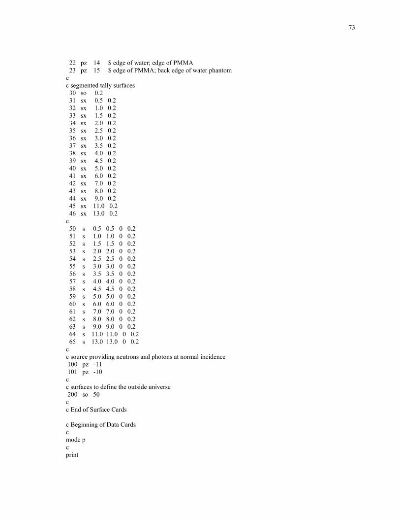
73
22 pz 14 $ edge of water; edge of PMMA 23 pz 15 $ edge of PMMA; back edge of water phantom c c segmented tally surfaces 30 so 0.2 31 sx 0.5 0.2 32 sx 1.0 0.2 33 sx 1.5 0.2 34 sx 2.0 0.2 35 sx 2.5 0.2 36 sx 3.0 0.2 37 sx 3.5 0.2 38 sx 4.0 0.2 39 sx 4.5 0.2 40 sx 5.0 0.2 41 sx 6.0 0.2 42 sx 7.0 0.2 43 sx 8.0 0.2 44 sx 9.0 0.2 45 sx 11.0 0.2 46 sx 13.0 0.2 c 50 s 0.5 0.5 0 0.2 51 s 1.0 1.0 0 0.2 52 s 1.5 1.5 0 0.2 53 s 2.0 2.0 0 0.2 54 s 2.5 2.5 0 0.2 55 s 3.0 3.0 0 0.2 56 s 3.5 3.5 0 0.2 57 s 4.0 4.0 0 0.2 58 s 4.5 4.5 0 0.2 59 s 5.0 5.0 0 0.2 60 s 6.0 6.0 0 0.2 61 s 7.0 7.0 0 0.2 62 s 8.0 8.0 0 0.2 63 s 9.0 9.0 0 0.2 64 s 11.0 11.0 0 0.2 65 s 13.0 13.0 0 0.2 c c source providing neutrons and photons at normal incidence 100 pz -11 101 pz -10 c c surfaces to define the outside universe 200 so 50 c c End of Surface Cards c Beginning of Data Cards c mode p c print
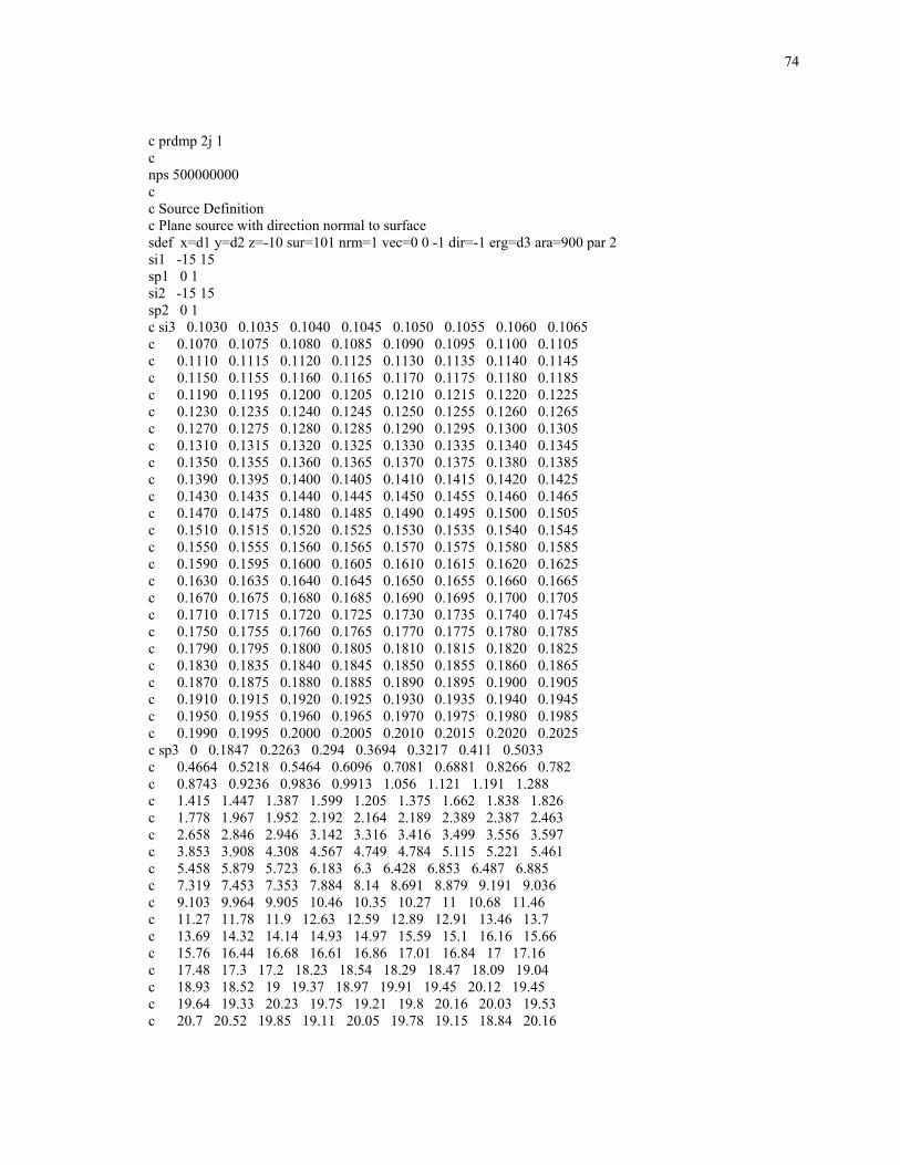
74
c prdmp 2j 1 c nps 500000000 c c Source Definition c Plane source with direction normal to surface sdef x=d1 y=d2 z=-10 sur=101 nrm=1 vec=0 0 -1 dir=-1 erg=d3 ara=900 par 2 si1 -15 15 sp1 0 1 si2 -15 15 sp2 0 1 c si3 0.1030 0.1035 0.1040 0.1045 0.1050 0.1055 0.1060 0.1065 c 0.1070 0.1075 0.1080 0.1085 0.1090 0.1095 0.1100 0.1105 c 0.1110 0.1115 0.1120 0.1125 0.1130 0.1135 0.1140 0.1145 c 0.1150 0.1155 0.1160 0.1165 0.1170 0.1175 0.1180 0.1185 c 0.1190 0.1195 0.1200 0.1205 0.1210 0.1215 0.1220 0.1225 c 0.1230 0.1235 0.1240 0.1245 0.1250 0.1255 0.1260 0.1265 c 0.1270 0.1275 0.1280 0.1285 0.1290 0.1295 0.1300 0.1305 c 0.1310 0.1315 0.1320 0.1325 0.1330 0.1335 0.1340 0.1345 c 0.1350 0.1355 0.1360 0.1365 0.1370 0.1375 0.1380 0.1385 c 0.1390 0.1395 0.1400 0.1405 0.1410 0.1415 0.1420 0.1425 c 0.1430 0.1435 0.1440 0.1445 0.1450 0.1455 0.1460 0.1465 c 0.1470 0.1475 0.1480 0.1485 0.1490 0.1495 0.1500 0.1505 c 0.1510 0.1515 0.1520 0.1525 0.1530 0.1535 0.1540 0.1545 c 0.1550 0.1555 0.1560 0.1565 0.1570 0.1575 0.1580 0.1585 c 0.1590 0.1595 0.1600 0.1605 0.1610 0.1615 0.1620 0.1625 c 0.1630 0.1635 0.1640 0.1645 0.1650 0.1655 0.1660 0.1665 c 0.1670 0.1675 0.1680 0.1685 0.1690 0.1695 0.1700 0.1705 c 0.1710 0.1715 0.1720 0.1725 0.1730 0.1735 0.1740 0.1745 c 0.1750 0.1755 0.1760 0.1765 0.1770 0.1775 0.1780 0.1785 c 0.1790 0.1795 0.1800 0.1805 0.1810 0.1815 0.1820 0.1825 c 0.1830 0.1835 0.1840 0.1845 0.1850 0.1855 0.1860 0.1865 c 0.1870 0.1875 0.1880 0.1885 0.1890 0.1895 0.1900 0.1905 c 0.1910 0.1915 0.1920 0.1925 0.1930 0.1935 0.1940 0.1945 c 0.1950 0.1955 0.1960 0.1965 0.1970 0.1975 0.1980 0.1985 c 0.1990 0.1995 0.2000 0.2005 0.2010 0.2015 0.2020 0.2025 c sp3 0 0.1847 0.2263 0.294 0.3694 0.3217 0.411 0.5033 c 0.4664 0.5218 0.5464 0.6096 0.7081 0.6881 0.8266 0.782 c 0.8743 0.9236 0.9836 0.9913 1.056 1.121 1.191 1.288 c 1.415 1.447 1.387 1.599 1.205 1.375 1.662 1.838 1.826 c 1.778 1.967 1.952 2.192 2.164 2.189 2.389 2.387 2.463 c 2.658 2.846 2.946 3.142 3.316 3.416 3.499 3.556 3.597 c 3.853 3.908 4.308 4.567 4.749 4.784 5.115 5.221 5.461 c 5.458 5.879 5.723 6.183 6.3 6.428 6.853 6.487 6.885 c 7.319 7.453 7.353 7.884 8.14 8.691 8.879 9.191 9.036 c 9.103 9.964 9.905 10.46 10.35 10.27 11 10.68 11.46 c 11.27 11.78 11.9 12.63 12.59 12.89 12.91 13.46 13.7 c 13.69 14.32 14.14 14.93 14.97 15.59 15.1 16.16 15.66 c 15.76 16.44 16.68 16.61 16.86 17.01 16.84 17 17.16 c 17.48 17.3 17.2 18.23 18.54 18.29 18.47 18.09 19.04 c 18.93 18.52 19 19.37 18.97 19.91 19.45 20.12 19.45 c 19.64 19.33 20.23 19.75 19.21 19.8 20.16 20.03 19.53 c 20.7 20.52 19.85 19.11 20.05 19.78 19.15 18.84 20.16
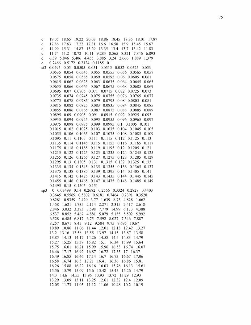
75
c 19.05 18.65 19.22 20.03 18.86 18.45 18.36 18.01 17.87 c 17.86 17.63 17.22 17.31 16.6 16.58 15.9 15.45 15.67 c 14.99 15.31 14.87 15.29 13.35 13.4 13.7 13.42 11.83 c 11.74 11.2 10.72 10.11 9.283 8.565 8.321 7.846 6.893 c 6.39 5.846 5.406 4.455 3.885 3.24 2.666 1.889 1.379 c 0.7466 0.5172 0.2124 0.1185 0 si3 0.0495 0.05 0.0505 0.051 0.0515 0.052 0.0525 0.053 0.0535 0.054 0.0545 0.055 0.0555 0.056 0.0565 0.057 0.0575 0.058 0.0585 0.059 0.0595 0.06 0.0605 0.061 0.0615 0.062 0.0625 0.063 0.0635 0.064 0.0645 0.065 0.0655 0.066 0.0665 0.067 0.0675 0.068 0.0685 0.069 0.0695 0.07 0.0705 0.071 0.0715 0.072 0.0725 0.073 0.0735 0.074 0.0745 0.075 0.0755 0.076 0.0765 0.077 0.0775 0.078 0.0785 0.079 0.0795 0.08 0.0805 0.081 0.0815 0.082 0.0825 0.083 0.0835 0.084 0.0845 0.085 0.0855 0.086 0.0865 0.087 0.0875 0.088 0.0885 0.089 0.0895 0.09 0.0905 0.091 0.0915 0.092 0.0925 0.093 0.0935 0.094 0.0945 0.095 0.0955 0.096 0.0965 0.097 0.0975 0.098 0.0985 0.099 0.0995 0.1 0.1005 0.101 0.1015 0.102 0.1025 0.103 0.1035 0.104 0.1045 0.105 0.1055 0.106 0.1065 0.107 0.1075 0.108 0.1085 0.109 0.1095 0.11 0.1105 0.111 0.1115 0.112 0.1125 0.113 0.1135 0.114 0.1145 0.115 0.1155 0.116 0.1165 0.117 0.1175 0.118 0.1185 0.119 0.1195 0.12 0.1205 0.121 0.1215 0.122 0.1225 0.123 0.1235 0.124 0.1245 0.125 0.1255 0.126 0.1265 0.127 0.1275 0.128 0.1285 0.129 0.1295 0.13 0.1305 0.131 0.1315 0.132 0.1325 0.133 0.1335 0.134 0.1345 0.135 0.1355 0.136 0.1365 0.137 0.1375 0.138 0.1385 0.139 0.1395 0.14 0.1405 0.141 0.1415 0.142 0.1425 0.143 0.1435 0.144 0.1445 0.145 0.1455 0.146 0.1465 0.147 0.1475 0.148 0.1485 0.149 0.1495 0.15 0.1505 0.151 sp3 0 0.03499 0.14 0.2682 0.2566 0.3324 0.2828 0.4403 0.3645 0.5569 0.5802 0.6181 0.7464 0.2391 0.3528 0.8281 0.9359 2.429 3.77 1.639 8.73 4.828 1.662 1.458 1.621 1.735 2.114 2.271 2.315 2.417 2.618 2.846 3.032 3.373 3.598 7.779 14.99 6.173 4.388 6.537 8.852 5.467 4.881 5.079 5.155 5.502 5.992 6.528 6.485 6.817 6.75 7.592 8.027 7.546 7.887 8.257 8.671 8.47 9.12 9.584 9.75 9.695 10.67 10.89 10.86 11.06 11.44 12.01 12.13 12.42 13.27 13.2 13.16 13.58 13.55 13.97 14.15 13.87 13.58 13.85 14.13 14.17 14.26 14.58 14.5 14.83 14.79 15.27 15.25 15.38 15.82 15.1 16.34 15.99 15.64 15.75 16.01 16.21 15.99 15.96 16.53 16.74 16.07 16.46 17.17 16.92 16.87 16.72 17.35 17 16.37 16.49 16.85 16.46 17.14 16.7 16.73 16.67 17.06 16.58 16.74 16.5 17.21 16.41 16.36 16.86 15.81 16.26 15.88 16.22 16.16 16.03 15.78 16.13 15.61 15.56 15.79 15.09 15.6 15.48 15.45 15.26 14.79 14.3 14.6 14.55 13.96 13.93 13.72 13.29 12.93 13.29 13.09 13.11 13.25 12.61 12.32 12.4 12.09 12.05 11.73 11.05 11.12 11.06 10.48 10.2 10.19
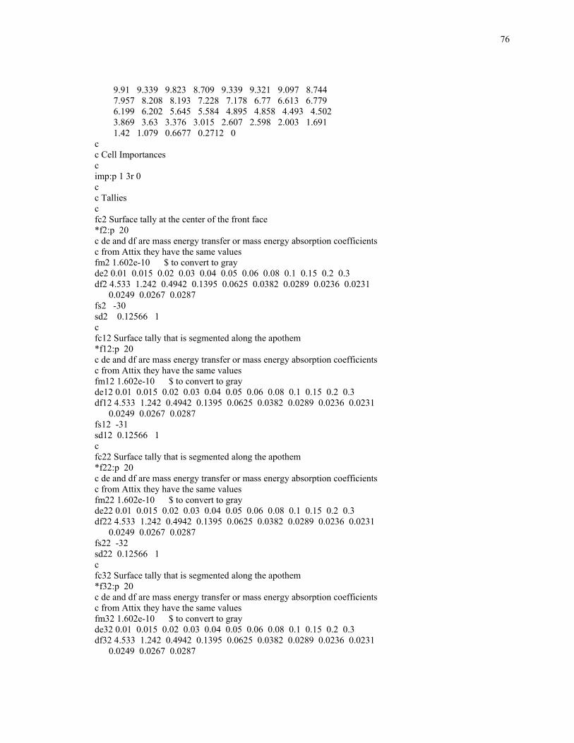
76
9.91 9.339 9.823 8.709 9.339 9.321 9.097 8.744 7.957 8.208 8.193 7.228 7.178 6.77 6.613 6.779 6.199 6.202 5.645 5.584 4.895 4.858 4.493 4.502 3.869 3.63 3.376 3.015 2.607 2.598 2.003 1.691 1.42 1.079 0.6677 0.2712 0 c c Cell Importances c imp:p 1 3r 0 c c Tallies c fc2 Surface tally at the center of the front face *f2:p 20 c de and df are mass energy transfer or mass energy absorption coefficients c from Attix they have the same values fm2 1.602e-10 $ to convert to gray de2 0.01 0.015 0.02 0.03 0.04 0.05 0.06 0.08 0.1 0.15 0.2 0.3 df2 4.533 1.242 0.4942 0.1395 0.0625 0.0382 0.0289 0.0236 0.0231 0.0249 0.0267 0.0287 fs2 -30 sd2 0.12566 1 c fc12 Surface tally that is segmented along the apothem *f12:p 20 c de and df are mass energy transfer or mass energy absorption coefficients c from Attix they have the same values fm12 1.602e-10 $ to convert to gray de12 0.01 0.015 0.02 0.03 0.04 0.05 0.06 0.08 0.1 0.15 0.2 0.3 df12 4.533 1.242 0.4942 0.1395 0.0625 0.0382 0.0289 0.0236 0.0231 0.0249 0.0267 0.0287 fs12 -31 sd12 0.12566 1 c fc22 Surface tally that is segmented along the apothem *f22:p 20 c de and df are mass energy transfer or mass energy absorption coefficients c from Attix they have the same values fm22 1.602e-10 $ to convert to gray de22 0.01 0.015 0.02 0.03 0.04 0.05 0.06 0.08 0.1 0.15 0.2 0.3 df22 4.533 1.242 0.4942 0.1395 0.0625 0.0382 0.0289 0.0236 0.0231 0.0249 0.0267 0.0287 fs22 -32 sd22 0.12566 1 c fc32 Surface tally that is segmented along the apothem *f32:p 20 c de and df are mass energy transfer or mass energy absorption coefficients c from Attix they have the same values fm32 1.602e-10 $ to convert to gray de32 0.01 0.015 0.02 0.03 0.04 0.05 0.06 0.08 0.1 0.15 0.2 0.3 df32 4.533 1.242 0.4942 0.1395 0.0625 0.0382 0.0289 0.0236 0.0231 0.0249 0.0267 0.0287
77
fs32 -33 sd32 0.12566 1 c fc42 Surface tally that is segmented along the apothem *f42:p 20 c de and df are mass energy transfer or mass energy absorption coefficients c from Attix they have the same values fm42 1.602e-10 $ to convert to gray de42 0.01 0.015 0.02 0.03 0.04 0.05 0.06 0.08 0.1 0.15 0.2 0.3 df42 4.533 1.242 0.4942 0.1395 0.0625 0.0382 0.0289 0.0236 0.0231 0.0249 0.0267 0.0287 fs42 -34 sd42 0.12566 1 c fc52 Surface tally that is segmented along the apothem *f52:p 20 c de and df are mass energy transfer or mass energy absorption coefficients c from Attix they have the same values fm52 1.602e-10 $ to convert to gray de52 0.01 0.015 0.02 0.03 0.04 0.05 0.06 0.08 0.1 0.15 0.2 0.3 df52 4.533 1.242 0.4942 0.1395 0.0625 0.0382 0.0289 0.0236 0.0231 0.0249 0.0267 0.0287 fs52 -35 sd52 0.12566 1 c fc62 Surface tally that is segmented along the apothem *f62:p 20 c de and df are mass energy transfer or mass energy absorption coefficients c from Attix they have the same values fm62 1.602e-10 $ to convert to gray de62 0.01 0.015 0.02 0.03 0.04 0.05 0.06 0.08 0.1 0.15 0.2 0.3 df62 4.533 1.242 0.4942 0.1395 0.0625 0.0382 0.0289 0.0236 0.0231 0.0249 0.0267 0.0287 fs62 -36 sd62 0.12566 1 c fc72 Surface tally that is segmented along the apothem *f72:p 20 c de and df are mass energy transfer or mass energy absorption coefficients c from Attix they have the same values fm72 1.602e-10 $ to convert to gray de72 0.01 0.015 0.02 0.03 0.04 0.05 0.06 0.08 0.1 0.15 0.2 0.3 df72 4.533 1.242 0.4942 0.1395 0.0625 0.0382 0.0289 0.0236 0.0231 0.0249 0.0267 0.0287 fs72 -37 sd72 0.12566 1 c fc82 Surface tally that is segmented along the apothem *f82:p 20 c de and df are mass energy transfer or mass energy absorption coefficients c from Attix they have the same values fm82 1.602e-10 $ to convert to gray de82 0.01 0.015 0.02 0.03 0.04 0.05 0.06 0.08 0.1 0.15 0.2 0.3
78
df82 4.533 1.242 0.4942 0.1395 0.0625 0.0382 0.0289 0.0236 0.0231 0.0249 0.0267 0.0287 fs82 -38 sd82 0.12566 1 c fc92 Surface tally that is segmented along the apothem *f92:p 20 c de and df are mass energy transfer or mass energy absorption coefficients c from Attix they have the same values fm92 1.602e-10 $ to convert to gray de92 0.01 0.015 0.02 0.03 0.04 0.05 0.06 0.08 0.1 0.15 0.2 0.3 df92 4.533 1.242 0.4942 0.1395 0.0625 0.0382 0.0289 0.0236 0.0231 0.0249 0.0267 0.0287 fs92 -39 sd92 0.12566 1 c fc102 Surface tally that is segmented along the apothem *f102:p 20 c de and df are mass energy transfer or mass energy absorption coefficients c from Attix they have the same values fm102 1.602e-10 $ to convert to gray de102 0.01 0.015 0.02 0.03 0.04 0.05 0.06 0.08 0.1 0.15 0.2 0.3 df102 4.533 1.242 0.4942 0.1395 0.0625 0.0382 0.0289 0.0236 0.0231 0.0249 0.0267 0.0287 fs102 -40 sd102 0.12566 1 c fc112 Surface tally that is segmented along the apothem *f112:p 20 c de and df are mass energy transfer or mass energy absorption coefficients c from Attix they have the same values fm112 1.602e-10 $ to convert to gray de112 0.01 0.015 0.02 0.03 0.04 0.05 0.06 0.08 0.1 0.15 0.2 0.3 df112 4.533 1.242 0.4942 0.1395 0.0625 0.0382 0.0289 0.0236 0.0231 0.0249 0.0267 0.0287 fs112 -41 sd112 0.12566 1 c fc122 Surface tally that is segmented along the apothem *f122:p 20 c de and df are mass energy transfer or mass energy absorption coefficients c from Attix they have the same values fm122 1.602e-10 $ to convert to gray de122 0.01 0.015 0.02 0.03 0.04 0.05 0.06 0.08 0.1 0.15 0.2 0.3 df122 4.533 1.242 0.4942 0.1395 0.0625 0.0382 0.0289 0.0236 0.0231 0.0249 0.0267 0.0287 fs122 -42 sd122 0.12566 1 c fc132 Surface tally that is segmented along the apothem *f132:p 20 c de and df are mass energy transfer or mass energy absorption coefficients c from Attix they have the same values
79
fm132 1.602e-10 $ to convert to gray de132 0.01 0.015 0.02 0.03 0.04 0.05 0.06 0.08 0.1 0.15 0.2 0.3 df132 4.533 1.242 0.4942 0.1395 0.0625 0.0382 0.0289 0.0236 0.0231 0.0249 0.0267 0.0287 fs132 -43 sd132 0.12566 1 c fc142 Surface tally that is segmented along the apothem *f142:p 20 c de and df are mass energy transfer or mass energy absorption coefficients c from Attix they have the same values fm142 1.602e-10 $ to convert to gray de142 0.01 0.015 0.02 0.03 0.04 0.05 0.06 0.08 0.1 0.15 0.2 0.3 df142 4.533 1.242 0.4942 0.1395 0.0625 0.0382 0.0289 0.0236 0.0231 0.0249 0.0267 0.0287 fs142 -44 sd142 0.12566 1 c fc152 Surface tally that is segmented along the apothem *f152:p 20 c de and df are mass energy transfer or mass energy absorption coefficients c from Attix they have the same values fm152 1.602e-10 $ to convert to gray de152 0.01 0.015 0.02 0.03 0.04 0.05 0.06 0.08 0.1 0.15 0.2 0.3 df152 4.533 1.242 0.4942 0.1395 0.0625 0.0382 0.0289 0.0236 0.0231 0.0249 0.0267 0.0287 fs152 -45 sd152 0.12566 1 c fc162 Surface tally that is segmented along the apothem *f162:p 20 c de and df are mass energy transfer or mass energy absorption coefficients c from Attix they have the same values fm162 1.602e-10 $ to convert to gray de162 0.01 0.015 0.02 0.03 0.04 0.05 0.06 0.08 0.1 0.15 0.2 0.3 df162 4.533 1.242 0.4942 0.1395 0.0625 0.0382 0.0289 0.0236 0.0231 0.0249 0.0267 0.0287 fs162 -46 sd162 0.12566 1 c fc172 Surface tally that is segmented along the diagonal *f172:p 20 c de and df are mass energy transfer or mass energy absorption coefficients c from Attix they have the same values fm172 1.602e-10 $ to convert to gray de172 0.01 0.015 0.02 0.03 0.04 0.05 0.06 0.08 0.1 0.15 0.2 0.3 df172 4.533 1.242 0.4942 0.1395 0.0625 0.0382 0.0289 0.0236 0.0231 0.0249 0.0267 0.0287 fs172 -50 sd172 0.12566 1 c fc182 Surface tally that is segmented along the diagonal *f182:p 20
80
c de and df are mass energy transfer or mass energy absorption coefficients c from Attix they have the same values fm182 1.602e-10 $ to convert to gray de182 0.01 0.015 0.02 0.03 0.04 0.05 0.06 0.08 0.1 0.15 0.2 0.3 df182 4.533 1.242 0.4942 0.1395 0.0625 0.0382 0.0289 0.0236 0.0231 0.0249 0.0267 0.0287 fs182 -51 sd182 0.12566 1 c fc192 Surface tally that is segmented along the diagonal *f192:p 20 c de and df are mass energy transfer or mass energy absorption coefficients c from Attix they have the same values fm192 1.602e-10 $ to convert to gray de192 0.01 0.015 0.02 0.03 0.04 0.05 0.06 0.08 0.1 0.15 0.2 0.3 df192 4.533 1.242 0.4942 0.1395 0.0625 0.0382 0.0289 0.0236 0.0231 0.0249 0.0267 0.0287 fs192 -52 sd192 0.12566 1 c fc202 Surface tally that is segmented along the diagonal *f202:p 20 c de and df are mass energy transfer or mass energy absorption coefficients c from Attix they have the same values fm202 1.602e-10 $ to convert to gray de202 0.01 0.015 0.02 0.03 0.04 0.05 0.06 0.08 0.1 0.15 0.2 0.3 df202 4.533 1.242 0.4942 0.1395 0.0625 0.0382 0.0289 0.0236 0.0231 0.0249 0.0267 0.0287 fs202 -53 sd202 0.12566 1 c fc212 Surface tally that is segmented along the diagonal *f212:p 20 c de and df are mass energy transfer or mass energy absorption coefficients c from Attix they have the same values fm212 1.602e-10 $ to convert to gray de212 0.01 0.015 0.02 0.03 0.04 0.05 0.06 0.08 0.1 0.15 0.2 0.3 df212 4.533 1.242 0.4942 0.1395 0.0625 0.0382 0.0289 0.0236 0.0231 0.0249 0.0267 0.0287 fs212 -54 sd212 0.12566 1 c fc222 Surface tally that is segmented along the diagonal *f222:p 20 c de and df are mass energy transfer or mass energy absorption coefficients c from Attix they have the same values fm222 1.602e-10 $ to convert to gray de222 0.01 0.015 0.02 0.03 0.04 0.05 0.06 0.08 0.1 0.15 0.2 0.3 df222 4.533 1.242 0.4942 0.1395 0.0625 0.0382 0.0289 0.0236 0.0231 0.0249 0.0267 0.0287 fs222 -55 sd222 0.12566 1 c
81
fc232 Surface tally that is segmented along the diagonal *f232:p 20 c de and df are mass energy transfer or mass energy absorption coefficients c from Attix they have the same values fm232 1.602e-10 $ to convert to gray de232 0.01 0.015 0.02 0.03 0.04 0.05 0.06 0.08 0.1 0.15 0.2 0.3 df232 4.533 1.242 0.4942 0.1395 0.0625 0.0382 0.0289 0.0236 0.0231 0.0249 0.0267 0.0287 fs232 -56 sd232 0.12566 1 c fc242 Surface tally that is segmented along the diagonal *f242:p 20 c de and df are mass energy transfer or mass energy absorption coefficients c from Attix they have the same values fm242 1.602e-10 $ to convert to gray de242 0.01 0.015 0.02 0.03 0.04 0.05 0.06 0.08 0.1 0.15 0.2 0.3 df242 4.533 1.242 0.4942 0.1395 0.0625 0.0382 0.0289 0.0236 0.0231 0.0249 0.0267 0.0287 fs242 -57 sd242 0.12566 1 c fc252 Surface tally that is segmented along the diagonal *f252:p 20 c mass energy transfer or mass energy absorption coefficients from Attix c they have the same values fm252 1.602e-10 $ to convert to gray de252 0.01 0.015 0.02 0.03 0.04 0.05 0.06 0.08 0.1 0.15 0.2 0.3 df252 4.533 1.242 0.4942 0.1395 0.0625 0.0382 0.0289 0.0236 0.0231 0.0249 0.0267 0.0287 fs252 -58 sd252 0.12566 1 c fc262 Surface tally that is segmented along the diagonal *f262:p 20 c de and df are mass energy transfer or mass energy absorption coefficients c from Attix they have the same values fm262 1.602e-10 $ to convert to gray de262 0.01 0.015 0.02 0.03 0.04 0.05 0.06 0.08 0.1 0.15 0.2 0.3 df262 4.533 1.242 0.4942 0.1395 0.0625 0.0382 0.0289 0.0236 0.0231 0.0249 0.0267 0.0287 fs262 -59 sd262 0.12566 1 c fc272 Surface tally that is segmented along the diagonal *f272:p 20 c de and df are mass energy transfer or mass energy absorption coefficients c from Attix they have the same values fm272 1.602e-10 $ to convert to gray de272 0.01 0.015 0.02 0.03 0.04 0.05 0.06 0.08 0.1 0.15 0.2 0.3 df272 4.533 1.242 0.4942 0.1395 0.0625 0.0382 0.0289 0.0236 0.0231 0.0249 0.0267 0.0287 fs272 -60
82
sd272 0.12566 1 c fc282 Surface tally that is segmented along the diagonal *f282:p 20 c de and df are mass energy transfer or mass energy absorption coefficients c from Attix they have the same values fm282 1.602e-10 $ to convert to gray de282 0.01 0.015 0.02 0.03 0.04 0.05 0.06 0.08 0.1 0.15 0.2 0.3 df282 4.533 1.242 0.4942 0.1395 0.0625 0.0382 0.0289 0.0236 0.0231 0.0249 0.0267 0.0287 fs282 -61 sd282 0.12566 1 c fc292 Surface tally that is segmented along the diagonal *f292:p 20 c de and df are mass energy transfer or mass energy absorption coefficients c from Attix they have the same values fm292 1.602e-10 $ to convert to gray de292 0.01 0.015 0.02 0.03 0.04 0.05 0.06 0.08 0.1 0.15 0.2 0.3 df292 4.533 1.242 0.4942 0.1395 0.0625 0.0382 0.0289 0.0236 0.0231 0.0249 0.0267 0.0287 fs292 -62 sd292 0.12566 1 c fc302 Surface tally that is segmented along the diagonal *f302:p 20 c de and df are mass energy transfer or mass energy absorption coefficients c from Attix they have the same values fm302 1.602e-10 $ to convert to gray de302 0.01 0.015 0.02 0.03 0.04 0.05 0.06 0.08 0.1 0.15 0.2 0.3 df302 4.533 1.242 0.4942 0.1395 0.0625 0.0382 0.0289 0.0236 0.0231 0.0249 0.0267 0.0287 fs302 -63 sd302 0.12566 1 c fc312 Surface tally that is segmented along the diagonal *f312:p 20 c de and df are mass energy transfer or mass energy absorption coefficients c from Attix they have the same values fm312 1.602e-10 $ to convert to gray de312 0.01 0.015 0.02 0.03 0.04 0.05 0.06 0.08 0.1 0.15 0.2 0.3 df312 4.533 1.242 0.4942 0.1395 0.0625 0.0382 0.0289 0.0236 0.0231 0.0249 0.0267 0.0287 fs312 -64 sd312 0.12566 1 c fc322 Surface tally that is segmented along the diagonal *f322:p 20 c de and df are mass energy transfer or mass energy absorption coefficients c from Attix they have the same values fm322 1.602e-10 $ to convert to gray de322 0.01 0.015 0.02 0.03 0.04 0.05 0.06 0.08 0.1 0.15 0.2 0.3 df322 4.533 1.242 0.4942 0.1395 0.0625 0.0382 0.0289 0.0236 0.0231
83
0.0249 0.0267 0.0287 fs322 -65 sd322 0.12566 1 c c Beginning of Material Data Cards c c PMMA c rho = 1.19 g/cc m1 001001 -0.0805259 001002 -0.0000120807 $ naturally occurring H 008016 -0.318853 008017 -0.000121453 008018 -0.000639228 $nat.O 006012 -0.593190 006013 -0.00665831 $ naturally occurring C c c Water c rho = 1.00 g/cc m2 001001 -0.1118772159 001002 -0.0000167841 $ naturally occurring H 008016 -0.88599230772 008017 -0.00033748028 008018 -0.001776212 $nat.O c c Air c density = 0.00120484 m3 007000 -0.790 008000 -0.210
84
Problem 6, Calibration of Neutron Detectors in a Bunker
Message: outp=p6o.o runtpe=p6r.r mctal=p6m.m Calibration of Neutron Detectors in a Bunker c 15.24 cm radius sphere to tally flux in approximating c 12" rem ball c c Beginning of Cell Cards c c Source 1 5 -15.100 -50 22 -23 c c Shadow Cone c iron section 5 3 -7.87 -60 3 -4 c polyethylene section 6 4 -0.94 -60 4 -5 c c Air inside room 10 2 -0.00120484 (60 3 -5 21 -24 31 -32): (5 -6 21 -24 31 -32 75 76 ): (2 -3 21 -22 31 -32): (2 -3 23 -24 31 -32): (2 -3 50 22 -23 31 -32) c c Bunker Wall 20 1 -2.3 (1 -2 20 -25 30 -33):(6 -7 20 -25 30 -33): (1 -7 20 -21 30 -33):(1 -7 24 -25 30 -33): (1 -7 20 -25 30 -31):(1 -7 20 -25 32 -33) c c Tally Cells c 50 2 -0.00120484 -75 c 51 2 -0.00120484 -76 c c Outside world 99 0 -1:7:-20:25:-30:33 c c Phoney cells to do surface tallies with 100 2 -0.00120484 -75 -40 101 2 -0.00120484 -75 40 102 2 -0.00120484 -76 -40 103 2 -0.00120484 -76 40 c c End of Cell Cards c Beginning of Surface Cards c 1 px -400 $ outside of bunker wall 2 px -350 $ inside of bunker wall 3 px 45 $ front edge of iron 4 px 65 $ back edge of iron; front edge of polyethylene 5 px 95 $ back edge of polyethylene
85
6 px 350 $ inside of bunker wall 7 px 400 $ outside of bunker wall c 20 py -400 $ outside of bunker wall 21 py -350 $ inside of bunker wall 22 py -0.25 $ bottom of source cylinder 23 py 0.25 $ top of source cylinder 24 py 350 $ inside of bunker wall 25 py 400 $ outside of bunker wall c 30 pz -375 $ outside of bunker wall 31 pz -325 $ inside of bunker wall 32 pz 325 $ inside of bunker wall 33 pz 375 $ outside of bunker wall c 40 pz 0 $ surface to cosine bin 41 px 165 $ segment of 40 for position 1 42 px 175 $ segment of 40 for position 1 43 px 295 $ segment of 40 for position 2 44 px 305 $ segment of 40 for position 2 45 py -5 $ segment of 40 46 py 5 $ segment of 40 c c source geometrically centered at 0,0,0 50 cy 0.25 c c tally spheres 75 sx 170 15.24 $ sphere 170 cm from source 76 sx 300 15.24 $ sphere 300 cm from source c c Shadow Cone 60 kx -15.0 2.16263e-2 +1 c c End of Surface Cards c Beginning of Data Cards c mode n c print c prdmp 2j 1 c nps 1000000000 c c Source Definition c Cylinder source with radius 0.25 cm and height 0.5 cm sdef pos=0 0 0 axs=0 1 0 rad=d1 ext=d2 erg=d3 par 1 si1 0.25 sp1 -21 1 si2 0.25 sp2 -21 0 si3 0.000000414 0.0000010 0.000010 0.000050 0.00010 0.00020 0.00040 0.00070 0.0010 0.0030 0.0060 0.010 0.020 0.040
86
0.060 0.080 0.10 0.15 0.20 0.25 0.30 0.35 0.40 0.45 0.50 0.55 0.60 0.70 0.80 0.90 1 1.2 1.4 1.6 1.8 2.0 2.3 2.6 3.0 3.5 4.0 4.5 5.0 6.0 7.0 8.0 9.0 10.0 11.0 12.0 13.0 14.0 15.0 16.0 sp3 0 0.31e-9 1.11e-8 1.27e-7 2.76e-7 7.82e-7 2.21e-6 4.53e-6 5.68e-6 5.51e-6 1.28e-4 2.30e-4 7.74e-4 2.17e-3 2.80e-3 3.29e-3 3.68e-3 1.05e-2 1.21e-2 1.33e-2 1.42e-2 1.49e-2 1.55e-2 1.60e-2 1.63e-2 1.66e-2 1.68e-2 3.38e-2 3.39e-2 3.37e-2 3.33e-2 6.46e-2 6.12e-2 5.73e-2 5.31e-2 4.88e-2 6.55e-2 5.67e-2 6.33e-2 6.21e-2 4.68e-2 3.49e-2 2.58e-2 3.30e-2 1.74e-2 9.01e-3 4.61e-3 2.33e-3 1.17e-3 5.83e-4 2.88e-4 1.42e-4 6.94e-5 0 c c Cell Importances c imp:n 1 3r 1 0 1 1 1 1 c imp:p 1 5r 1 0 1 c c Tallies c c Spherical detectors to compare c cosine bins will not work with this either c fc4 Spherical detector at position 1: 170,0,0 f4:n (100 101) e4 0.000000414 0.0000010 0.000010 0.000050 0.00010 0.00020 0.00040 0.00070 0.0010 0.0030 0.0060 0.010 0.020 0.040 0.060 0.080 0.10 0.15 0.20 0.25 0.30 0.35 0.40 0.45 0.50 0.55 0.60 0.70 0.80 0.90 1 1.2 1.4 1.6 1.8 2.0 2.3 2.6 3.0 3.5 4.0 4.5 5.0 6.0 7.0 8.0 9.0 10.0 11.0 12.0 13.0 14.0 15.0 16.0 c fc14 Spherical detector at position2: 300,0,0 f14:n (102 103) e14 0.000000414 0.0000010 0.000010 0.000050 0.00010 0.00020 0.00040 0.00070 0.0010 0.0030 0.0060 0.010 0.020 0.040 0.060 0.080 0.10 0.15 0.20 0.25 0.30 0.35 0.40 0.45 0.50 0.55 0.60 0.70 0.80 0.90 1 1.2 1.4 1.6 1.8 2.0 2.3 2.6 3.0 3.5 4.0 4.5 5.0 6.0 7.0 8.0 9.0 10.0 11.0 12.0 13.0 14.0 15.0 16.0 c fc1 Planar surfaces for cosine binning position 1: 170,0,0 position 2: 300,0,0 f1:n 40 fs1 -75 sd1 62.8318 1 e1 0.000000414 0.0000010 0.000010 0.000050 0.00010 0.00020 0.00040 0.00070 0.0010 0.0030 0.0060 0.010 0.020 0.040 0.060 0.080 0.10 0.15 0.20 0.25 0.30 0.35 0.40 0.45 0.50 0.55 0.60 0.70 0.80 0.90 1 1.2 1.4 1.6 1.8 2.0 2.3 2.6 3.0 3.5 4.0 4.5 5.0 6.0 7.0 8.0 9.0 10.0 11.0 12.0 13.0 14.0 15.0 16.0
87
c1 -0.866 -0.5 0 0.5 0.866 1 c f11:n 40 fs11 -76 sd11 62.8318 1 e11 0.000000414 0.0000010 0.000010 0.000050 0.00010 0.00020 0.00040 0.00070 0.0010 0.0030 0.0060 0.010 0.020 0.040 0.060 0.080 0.10 0.15 0.20 0.25 0.30 0.35 0.40 0.45 0.50 0.55 0.60 0.70 0.80 0.90 1 1.2 1.4 1.6 1.8 2.0 2.3 2.6 3.0 3.5 4.0 4.5 5.0 6.0 7.0 8.0 9.0 10.0 11.0 12.0 13.0 14.0 15.0 16.0 c11 -0.866 -0.5 0 0.5 0.866 1 c c Beginning of Material Data Cards c c Concrete c rho = 2.3 g/cc m1 001001 0.11698245 001002 0.00001755 008016 0.60796842 008017 0.000231579 014028 0.25344804 014029 0.01283316 014030 0.0085188 c c Air c rho = 0.00120484 g/cc m2 006012 -0.00012521867138 006013 -0.00000140552862 007014 -0.762280494675 007015 -0.0028001953254 008016 -0.23470328576 008017 -0.000089400020638 c c Iron c rho = 7.87 g/cc m3 026054 0.05845 026056 0.91754 026057 0.02119 026058 0.00282 c c Polyethylene c rho = 0.94 g/cc m4 006012 0.9889 006013 0.0111 001001 1.9997 001002 0.0003 c c Californium 252 c rho = 15.100 m5 098252 1
88
Problem 7, Pulse Height Distributions of a Germanium Spectrometer in the Energy Range Below 1 MeV
Message: outp=p7.o runtpe=p7.r mctal=p7.m Germanium Detector - 15 keV c Beginning of Cell Cards c c Source - cylinder filled with air c use surface 2 on cell 1 with a circular plane source in sdef 1 1 -0.00120484 -50 1 -2 c c Be window 5 4 -1.848 -56 3 -4 c c Cryostat 10 3 -2.70 (-51 52 3 -11):(-51 56 3 -4):(-51 10 -11) c c Al Holder 15 3 -2.70 (53 -55 5 -8):(8 -9 -55) c c Ge Crystal c dead layer 20 2 -5.323 (-53 54 5 -8):(-53 5 -6):(-53 7 -8) c core 21 2 -5.323 -54 6 -7 c c Vacuum inside cryostat 25 0 (-52 9 -10):(-52 55 5 -9):(-52 4 -5) c c Air outside cryostat 30 1 -0.00120484 (11 -100):(-100 51 3 -11):(-100 2 -3): (-100 50 1 -2):(-1 -100) c c Outside world 99 0 100 c c End of Cell Cards c Beginning of Surface Cards c 1 px -21 $ arbitrary farthest edge of source disk 2 px -20 $ closest edge of source disk c Assume this will be a disk surface source c 3 px 0 $ top of cryostat; front edge of Be window 4 px 0.15 $ back edge of Be window; thickness of cryostat 5 px 0.65 $ front edge of Germanium detector 6 px 0.66 $ top of dead layer 7 px 2.14 $ bottom dead layer 8 px 2.15 $ back edge of Germanium detector 9 px 2.2 $ bottom of Al holder 10 px 5.65 $ thickness of cryostat 11 px 5.8 $ bottom of cryotstat
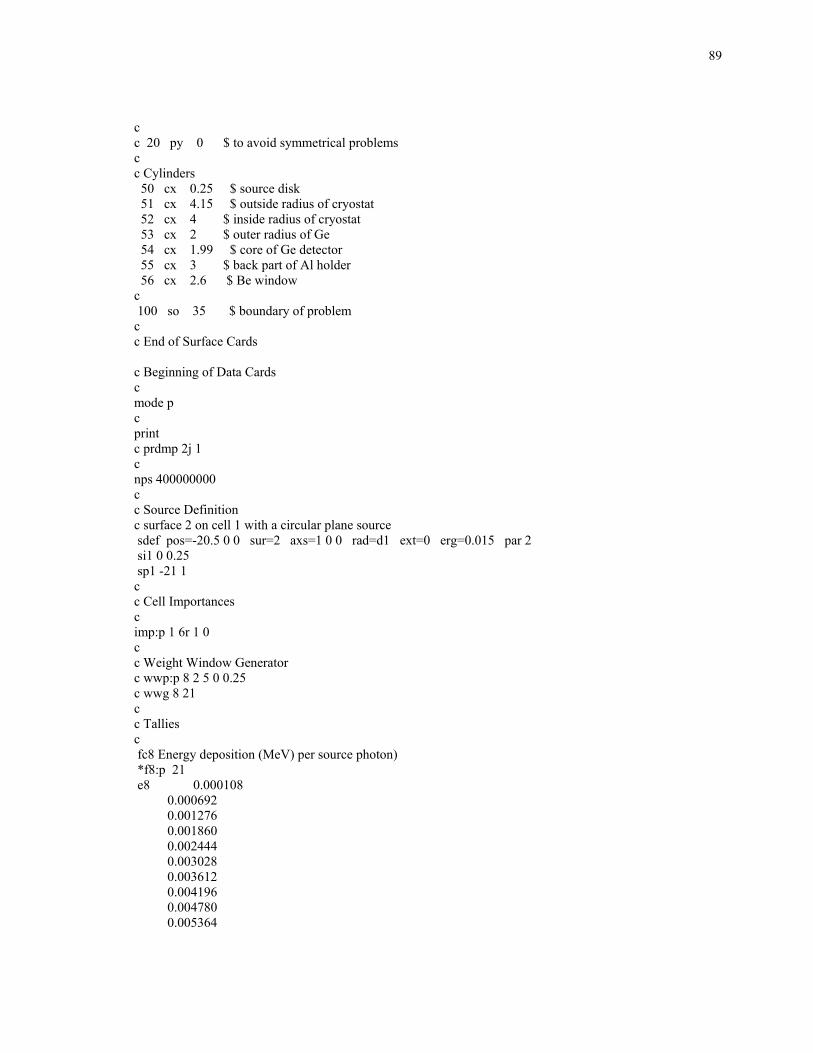
89
c c 20 py 0 $ to avoid symmetrical problems c c Cylinders 50 cx 0.25 $ source disk 51 cx 4.15 $ outside radius of cryostat 52 cx 4 $ inside radius of cryostat 53 cx 2 $ outer radius of Ge 54 cx 1.99 $ core of Ge detector 55 cx 3 $ back part of Al holder 56 cx 2.6 $ Be window c 100 so 35 $ boundary of problem c c End of Surface Cards c Beginning of Data Cards c mode p c print c prdmp 2j 1 c nps 400000000 c c Source Definition c surface 2 on cell 1 with a circular plane source sdef pos=-20.5 0 0 sur=2 axs=1 0 0 rad=d1 ext=0 erg=0.015 par 2 si1 0 0.25 sp1 -21 1 c c Cell Importances c imp:p 1 6r 1 0 c c Weight Window Generator c wwp:p 8 2 5 0 0.25 c wwg 8 21 c c Tallies c fc8 Energy deposition (MeV) per source photon) *f8:p 21 e8 0.000108 0.000692 0.001276 0.001860 0.002444 0.003028 0.003612 0.004196 0.004780 0.005364
90
0.005948 0.006532 0.007116 0.007700 0.008284 0.008868 0.009452 0.010036 0.010620 0.011204 0.011788 0.012372 0.012956 0.013540 0.014124 0.014708 0.015292 0.015876 c fc18 Pulses f18:p 21 e18 0.000108 0.000692 0.001276 0.001860 0.002444 0.003028 0.003612 0.004196 0.004780 0.005364 0.005948 0.006532 0.007116 0.007700 0.008284 0.008868 0.009452 0.010036 0.010620 0.011204 0.011788 0.012372 0.012956 0.013540 0.014124 0.014708 0.015292 0.015876 c c Beginning of Material Data Cards c c Air
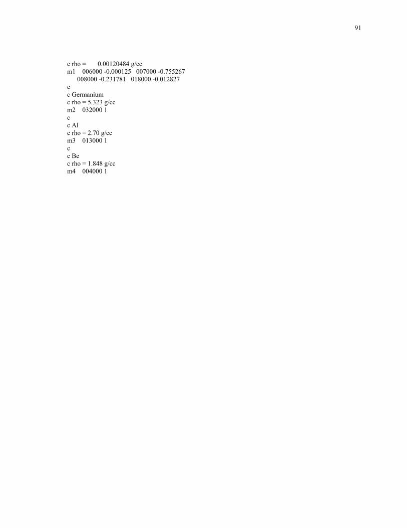
91
c rho = 0.00120484 g/cc m1 006000 -0.000125 007000 -0.755267 008000 -0.231781 018000 -0.012827 c c Germanium c rho = 5.323 g/cc m2 032000 1 c c Al c rho = 2.70 g/cc m3 013000 1 c c Be c rho = 1.848 g/cc m4 004000 1
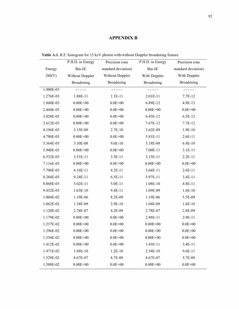
92
APPENDIX B
Table A.1. R.F. histogram for 15 keV photon with/without Doppler broadening feature.
Energy
(MeV)
P.H.D. in Energy
Bin δE
Without Doppler
Broadening
Precision (one
standard deviation)
Without Doppler
Broadening
P.H.D. in Energy
Bin δE
With Doppler
Broadening
Precision (one
standard deviation)
With Doppler
Broadening
1.000E-03 - - - - - - - - - - - - - - - - - - - -
1.276E-03 1.88E-11 1.1E-11 2.01E-11 7.7E-12
1.860E-03 0.00E+00 0.0E+00 6.89E-12 4.9E-12
2.444E-03 0.00E+00 0.0E+00 0.00E+00 0.0E+00
3.028E-03 0.00E+00 0.0E+00 6.45E-12 6.5E-12
3.612E-03 0.00E+00 0.0E+00 7.67E-12 7.7E-12
4.196E-03 3.15E-09 2.7E-10 3.62E-09 1.9E-10
4.780E-03 0.00E+00 0.0E+00 5.81E-11 2.6E-11
5.364E-03 3.10E-08 9.6E-10 3.18E-08 6.4E-10
5.948E-03 0.00E+00 0.0E+00 7.00E-11 3.1E-11
6.532E-03 3.51E-11 3.5E-11 3.15E-11 2.2E-11
7.116E-03 0.00E+00 0.0E+00 0.00E+00 0.0E+00
7.700E-03 4.16E-11 4.2E-11 3.64E-11 2.6E-11
8.284E-03 9.24E-11 6.5E-11 5.97E-11 3.4E-11
8.868E-03 5.02E-11 5.0E-11 1.08E-10 4.8E-11
9.452E-03 1.63E-10 9.4E-11 1.09E-09 1.6E-10
1.004E-02 1.19E-06 8.2E-09 1.19E-06 5.5E-09
1.062E-02 1.34E-09 2.9E-10 1.04E-09 1.6E-10
1.120E-02 2.76E-07 4.2E-09 2.78E-07 2.8E-09
1.179E-02 0.00E+00 0.0E+00 2.88E-11 2.9E-11
1.237E-02 0.00E+00 0.0E+00 0.00E+00 0.0E+00
1.296E-02 0.00E+00 0.0E+00 0.00E+00 0.0E+00
1.354E-02 0.00E+00 0.0E+00 0.00E+00 0.0E+00
1.412E-02 0.00E+00 0.0E+00 3.43E-11 3.4E-11
1.471E-02 1.68E-10 1.2E-10 2.54E-10 9.6E-11
1.529E-02 8.67E-07 8.7E-09 8.67E-07 5.7E-09
1.588E-02 0.00E+00 0.0E+00 0.00E+00 0.0E+00
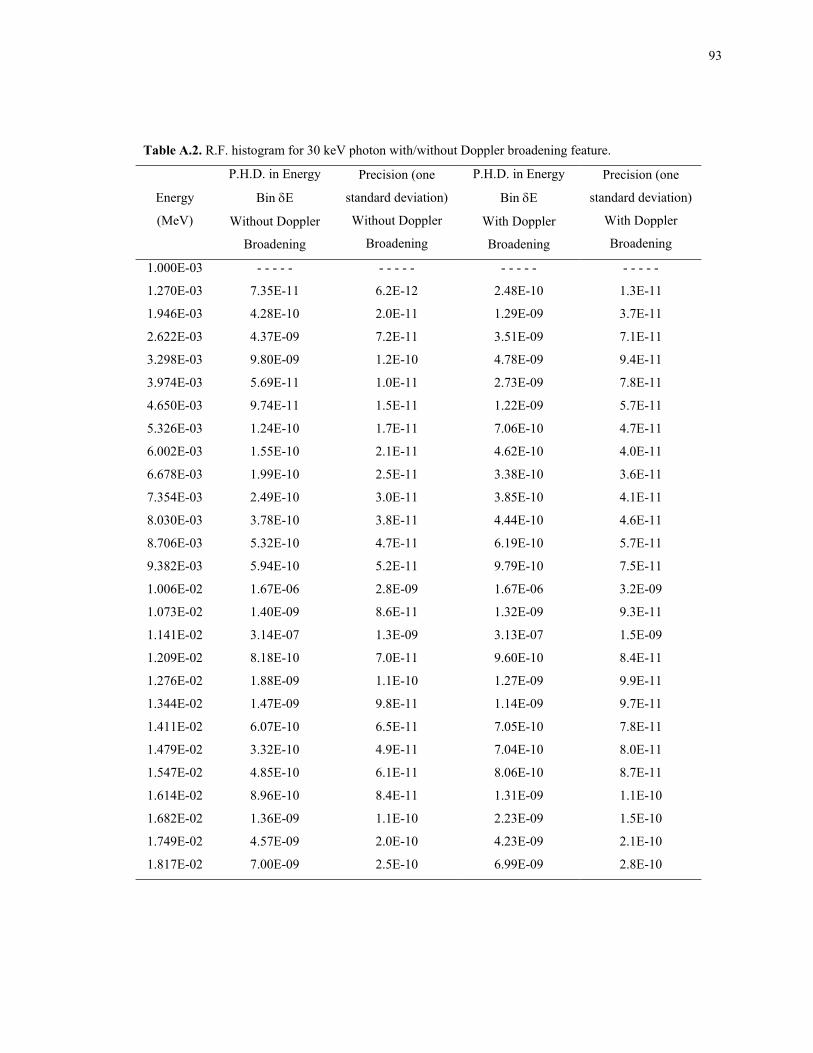
93
Table A.2. R.F. histogram for 30 keV photon with/without Doppler broadening feature.
Energy
(MeV)
P.H.D. in Energy
Bin δE
Without Doppler
Broadening
Precision (one
standard deviation)
Without Doppler
Broadening
P.H.D. in Energy
Bin δE
With Doppler
Broadening
Precision (one
standard deviation)
With Doppler
Broadening
1.000E-03 - - - - - - - - - - - - - - - - - - - -
1.270E-03 7.35E-11 6.2E-12 2.48E-10 1.3E-11
1.946E-03 4.28E-10 2.0E-11 1.29E-09 3.7E-11
2.622E-03 4.37E-09 7.2E-11 3.51E-09 7.1E-11
3.298E-03 9.80E-09 1.2E-10 4.78E-09 9.4E-11
3.974E-03 5.69E-11 1.0E-11 2.73E-09 7.8E-11
4.650E-03 9.74E-11 1.5E-11 1.22E-09 5.7E-11
5.326E-03 1.24E-10 1.7E-11 7.06E-10 4.7E-11
6.002E-03 1.55E-10 2.1E-11 4.62E-10 4.0E-11
6.678E-03 1.99E-10 2.5E-11 3.38E-10 3.6E-11
7.354E-03 2.49E-10 3.0E-11 3.85E-10 4.1E-11
8.030E-03 3.78E-10 3.8E-11 4.44E-10 4.6E-11
8.706E-03 5.32E-10 4.7E-11 6.19E-10 5.7E-11
9.382E-03 5.94E-10 5.2E-11 9.79E-10 7.5E-11
1.006E-02 1.67E-06 2.8E-09 1.67E-06 3.2E-09
1.073E-02 1.40E-09 8.6E-11 1.32E-09 9.3E-11
1.141E-02 3.14E-07 1.3E-09 3.13E-07 1.5E-09
1.209E-02 8.18E-10 7.0E-11 9.60E-10 8.4E-11
1.276E-02 1.88E-09 1.1E-10 1.27E-09 9.9E-11
1.344E-02 1.47E-09 9.8E-11 1.14E-09 9.7E-11
1.411E-02 6.07E-10 6.5E-11 7.05E-10 7.8E-11
1.479E-02 3.32E-10 4.9E-11 7.04E-10 8.0E-11
1.547E-02 4.85E-10 6.1E-11 8.06E-10 8.7E-11
1.614E-02 8.96E-10 8.4E-11 1.31E-09 1.1E-10
1.682E-02 1.36E-09 1.1E-10 2.23E-09 1.5E-10
1.749E-02 4.57E-09 2.0E-10 4.23E-09 2.1E-10
1.817E-02 7.00E-09 2.5E-10 6.99E-09 2.8E-10
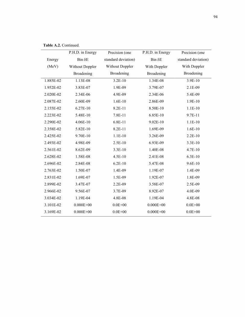
94
Table A.2. Continued.
Energy
(MeV)
P.H.D. in Energy
Bin δE
Without Doppler
Broadening
Precision (one
standard deviation)
Without Doppler
Broadening
P.H.D. in Energy
Bin δE
With Doppler
Broadening
Precision (one
standard deviation)
With Doppler
Broadening
1.885E-02 1.13E-08 3.2E-10 1.34E-08 3.9E-10
1.952E-02 3.83E-07 1.9E-09 3.79E-07 2.1E-09
2.020E-02 2.34E-06 4.9E-09 2.34E-06 5.4E-09
2.087E-02 2.60E-09 1.6E-10 2.86E-09 1.9E-10
2.155E-02 6.27E-10 8.2E-11 8.50E-10 1.1E-10
2.223E-02 5.48E-10 7.8E-11 6.85E-10 9.7E-11
2.290E-02 4.06E-10 6.8E-11 9.02E-10 1.1E-10
2.358E-02 5.82E-10 8.2E-11 1.69E-09 1.6E-10
2.425E-02 9.70E-10 1.1E-10 3.26E-09 2.2E-10
2.493E-02 4.98E-09 2.5E-10 6.93E-09 3.3E-10
2.561E-02 8.62E-09 3.3E-10 1.40E-08 4.7E-10
2.628E-02 1.58E-08 4.5E-10 2.41E-08 6.3E-10
2.696E-02 2.84E-08 6.2E-10 5.47E-08 9.6E-10
2.763E-02 1.50E-07 1.4E-09 1.19E-07 1.4E-09
2.831E-02 1.69E-07 1.5E-09 1.92E-07 1.8E-09
2.899E-02 3.47E-07 2.2E-09 3.58E-07 2.5E-09
2.966E-02 9.56E-07 3.7E-09 8.92E-07 4.0E-09
3.034E-02 1.19E-04 4.8E-08 1.19E-04 4.8E-08
3.101E-02 0.000E+00 0.0E+00 0.000E+00 0.0E+00
3.169E-02 0.000E+00 0.0E+00 0.000E+00 0.0E+00
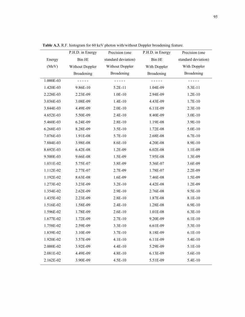
95
Table A.3. R.F. histogram for 60 keV photon with/without Doppler broadening feature.
Energy
(MeV)
P.H.D. in Energy
Bin δE
Without Doppler
Broadening
Precision (one
standard deviation)
Without Doppler
Broadening
P.H.D. in Energy
Bin δE
With Doppler
Broadening
Precision (one
standard deviation)
With Doppler
Broadening
1.000E-03 - - - - - - - - - - - - - - - - - - - -
1.420E-03 9.86E-10 5.2E-11 1.04E-09 5.3E-11
2.228E-03 2.23E-09 1.0E-10 2.94E-09 1.2E-10
3.036E-03 3.08E-09 1.4E-10 4.43E-09 1.7E-10
3.844E-03 4.49E-09 2.0E-10 6.11E-09 2.3E-10
4.652E-03 5.50E-09 2.4E-10 8.40E-09 3.0E-10
5.460E-03 6.24E-09 2.8E-10 1.19E-08 3.9E-10
6.268E-03 8.28E-09 3.5E-10 1.72E-08 5.0E-10
7.076E-03 1.91E-08 5.7E-10 2.68E-08 6.7E-10
7.884E-03 3.98E-08 8.6E-10 4.20E-08 8.9E-10
8.692E-03 6.42E-08 1.2E-09 6.02E-08 1.1E-09
9.500E-03 9.66E-08 1.5E-09 7.95E-08 1.3E-09
1.031E-02 5.75E-07 3.8E-09 5.36E-07 3.6E-09
1.112E-02 2.77E-07 2.7E-09 1.78E-07 2.2E-09
1.192E-02 8.63E-08 1.6E-09 7.46E-08 1.5E-09
1.273E-02 3.23E-09 3.2E-10 4.42E-08 1.2E-09
1.354E-02 2.62E-09 2.9E-10 2.76E-08 9.5E-10
1.435E-02 2.23E-09 2.8E-10 1.87E-08 8.1E-10
1.516E-02 1.58E-09 2.4E-10 1.28E-08 6.9E-10
1.596E-02 1.78E-09 2.6E-10 1.01E-08 6.3E-10
1.677E-02 1.72E-09 2.7E-10 9.20E-09 6.1E-10
1.758E-02 2.59E-09 3.3E-10 6.61E-09 5.3E-10
1.839E-02 3.10E-09 3.7E-10 8.18E-09 6.1E-10
1.920E-02 3.57E-09 4.1E-10 6.11E-09 5.4E-10
2.000E-02 3.92E-09 4.4E-10 5.29E-09 5.1E-10
2.081E-02 4.49E-09 4.8E-10 6.13E-09 5.6E-10
2.162E-02 3.90E-09 4.5E-10 5.51E-09 5.4E-10
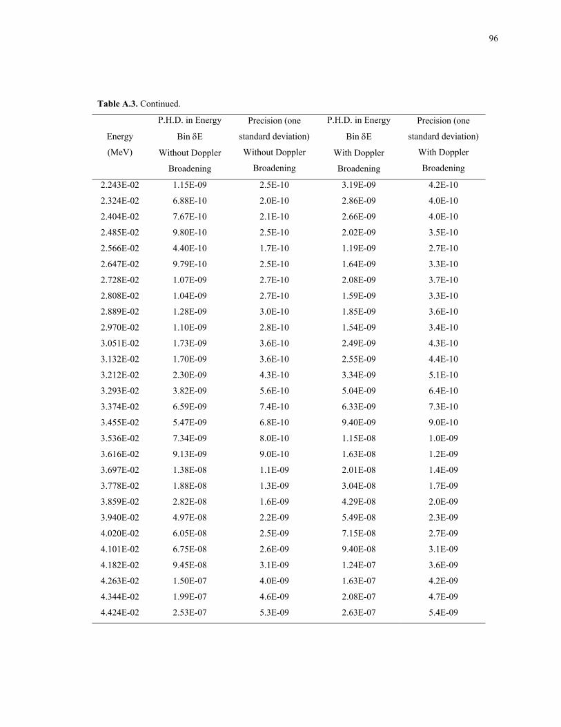
96
Table A.3. Continued.
Energy
(MeV)
P.H.D. in Energy
Bin δE
Without Doppler
Broadening
Precision (one
standard deviation)
Without Doppler
Broadening
P.H.D. in Energy
Bin δE
With Doppler
Broadening
Precision (one
standard deviation)
With Doppler
Broadening
2.243E-02 1.15E-09 2.5E-10 3.19E-09 4.2E-10
2.324E-02 6.88E-10 2.0E-10 2.86E-09 4.0E-10
2.404E-02 7.67E-10 2.1E-10 2.66E-09 4.0E-10
2.485E-02 9.80E-10 2.5E-10 2.02E-09 3.5E-10
2.566E-02 4.40E-10 1.7E-10 1.19E-09 2.7E-10
2.647E-02 9.79E-10 2.5E-10 1.64E-09 3.3E-10
2.728E-02 1.07E-09 2.7E-10 2.08E-09 3.7E-10
2.808E-02 1.04E-09 2.7E-10 1.59E-09 3.3E-10
2.889E-02 1.28E-09 3.0E-10 1.85E-09 3.6E-10
2.970E-02 1.10E-09 2.8E-10 1.54E-09 3.4E-10
3.051E-02 1.73E-09 3.6E-10 2.49E-09 4.3E-10
3.132E-02 1.70E-09 3.6E-10 2.55E-09 4.4E-10
3.212E-02 2.30E-09 4.3E-10 3.34E-09 5.1E-10
3.293E-02 3.82E-09 5.6E-10 5.04E-09 6.4E-10
3.374E-02 6.59E-09 7.4E-10 6.33E-09 7.3E-10
3.455E-02 5.47E-09 6.8E-10 9.40E-09 9.0E-10
3.536E-02 7.34E-09 8.0E-10 1.15E-08 1.0E-09
3.616E-02 9.13E-09 9.0E-10 1.63E-08 1.2E-09
3.697E-02 1.38E-08 1.1E-09 2.01E-08 1.4E-09
3.778E-02 1.88E-08 1.3E-09 3.04E-08 1.7E-09
3.859E-02 2.82E-08 1.6E-09 4.29E-08 2.0E-09
3.940E-02 4.97E-08 2.2E-09 5.49E-08 2.3E-09
4.020E-02 6.05E-08 2.5E-09 7.15E-08 2.7E-09
4.101E-02 6.75E-08 2.6E-09 9.40E-08 3.1E-09
4.182E-02 9.45E-08 3.1E-09 1.24E-07 3.6E-09
4.263E-02 1.50E-07 4.0E-09 1.63E-07 4.2E-09
4.344E-02 1.99E-07 4.6E-09 2.08E-07 4.7E-09
4.424E-02 2.53E-07 5.3E-09 2.63E-07 5.4E-09
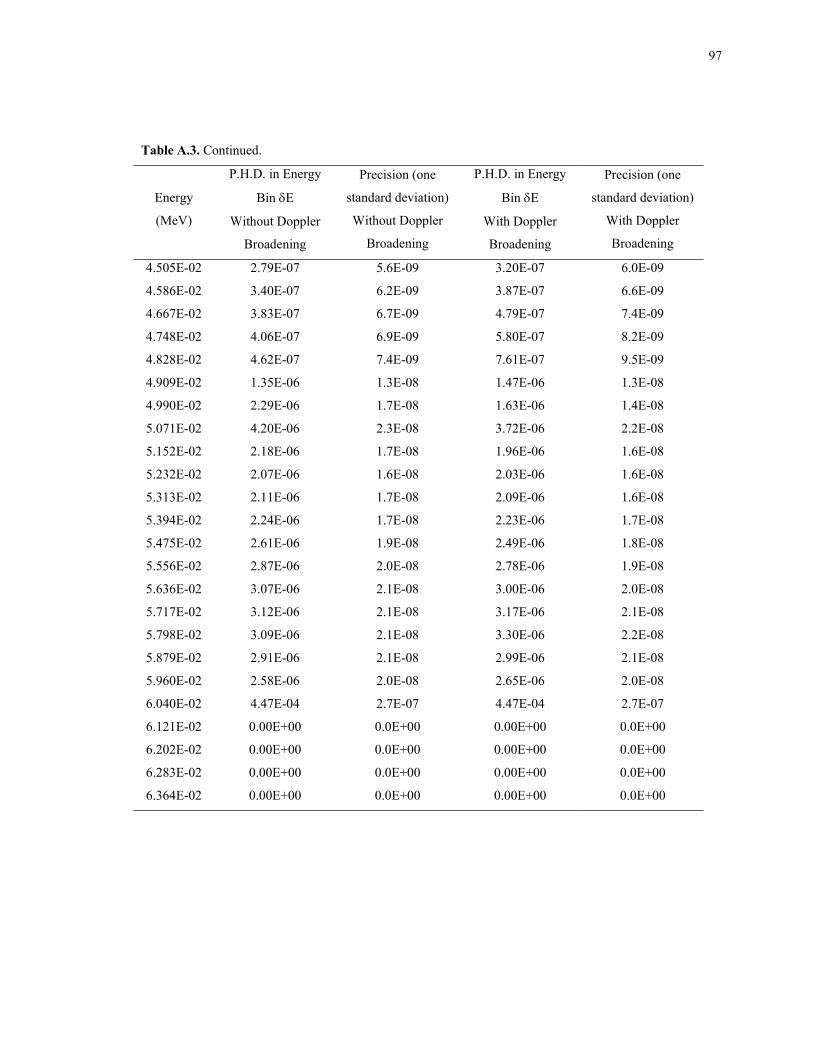
97
Table A.3. Continued.
Energy
(MeV)
P.H.D. in Energy
Bin δE
Without Doppler
Broadening
Precision (one
standard deviation)
Without Doppler
Broadening
P.H.D. in Energy
Bin δE
With Doppler
Broadening
Precision (one
standard deviation)
With Doppler
Broadening
4.505E-02 2.79E-07 5.6E-09 3.20E-07 6.0E-09
4.586E-02 3.40E-07 6.2E-09 3.87E-07 6.6E-09
4.667E-02 3.83E-07 6.7E-09 4.79E-07 7.4E-09
4.748E-02 4.06E-07 6.9E-09 5.80E-07 8.2E-09
4.828E-02 4.62E-07 7.4E-09 7.61E-07 9.5E-09
4.909E-02 1.35E-06 1.3E-08 1.47E-06 1.3E-08
4.990E-02 2.29E-06 1.7E-08 1.63E-06 1.4E-08
5.071E-02 4.20E-06 2.3E-08 3.72E-06 2.2E-08
5.152E-02 2.18E-06 1.7E-08 1.96E-06 1.6E-08
5.232E-02 2.07E-06 1.6E-08 2.03E-06 1.6E-08
5.313E-02 2.11E-06 1.7E-08 2.09E-06 1.6E-08
5.394E-02 2.24E-06 1.7E-08 2.23E-06 1.7E-08
5.475E-02 2.61E-06 1.9E-08 2.49E-06 1.8E-08
5.556E-02 2.87E-06 2.0E-08 2.78E-06 1.9E-08
5.636E-02 3.07E-06 2.1E-08 3.00E-06 2.0E-08
5.717E-02 3.12E-06 2.1E-08 3.17E-06 2.1E-08
5.798E-02 3.09E-06 2.1E-08 3.30E-06 2.2E-08
5.879E-02 2.91E-06 2.1E-08 2.99E-06 2.1E-08
5.960E-02 2.58E-06 2.0E-08 2.65E-06 2.0E-08
6.040E-02 4.47E-04 2.7E-07 4.47E-04 2.7E-07
6.121E-02 0.00E+00 0.0E+00 0.00E+00 0.0E+00
6.202E-02 0.00E+00 0.0E+00 0.00E+00 0.0E+00
6.283E-02 0.00E+00 0.0E+00 0.00E+00 0.0E+00
6.364E-02 0.00E+00 0.0E+00 0.00E+00 0.0E+00
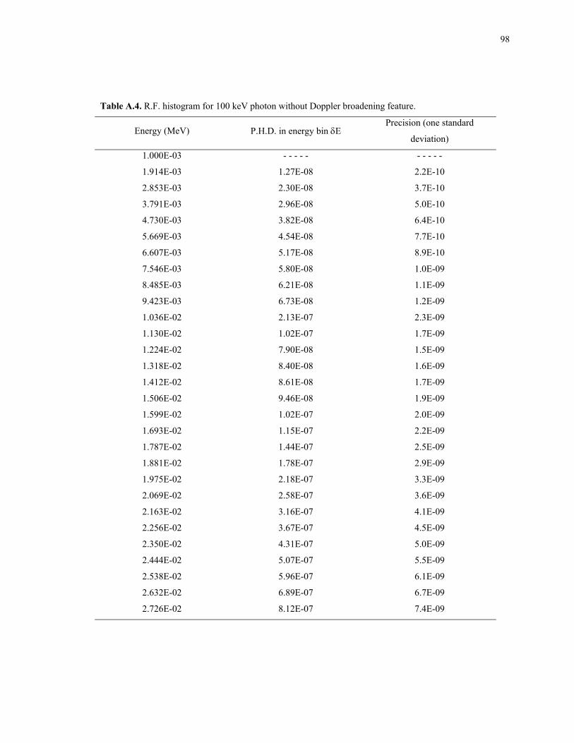
98
Table A.4. R.F. histogram for 100 keV photon without Doppler broadening feature.
Energy (MeV) P.H.D. in energy bin δE Precision (one standard
deviation)
1.000E-03 - - - - - - - - - -
1.914E-03 1.27E-08 2.2E-10
2.853E-03 2.30E-08 3.7E-10
3.791E-03 2.96E-08 5.0E-10
4.730E-03 3.82E-08 6.4E-10
5.669E-03 4.54E-08 7.7E-10
6.607E-03 5.17E-08 8.9E-10
7.546E-03 5.80E-08 1.0E-09
8.485E-03 6.21E-08 1.1E-09
9.423E-03 6.73E-08 1.2E-09
1.036E-02 2.13E-07 2.3E-09
1.130E-02 1.02E-07 1.7E-09
1.224E-02 7.90E-08 1.5E-09
1.318E-02 8.40E-08 1.6E-09
1.412E-02 8.61E-08 1.7E-09
1.506E-02 9.46E-08 1.9E-09
1.599E-02 1.02E-07 2.0E-09
1.693E-02 1.15E-07 2.2E-09
1.787E-02 1.44E-07 2.5E-09
1.881E-02 1.78E-07 2.9E-09
1.975E-02 2.18E-07 3.3E-09
2.069E-02 2.58E-07 3.6E-09
2.163E-02 3.16E-07 4.1E-09
2.256E-02 3.67E-07 4.5E-09
2.350E-02 4.31E-07 5.0E-09
2.444E-02 5.07E-07 5.5E-09
2.538E-02 5.96E-07 6.1E-09
2.632E-02 6.89E-07 6.7E-09
2.726E-02 8.12E-07 7.4E-09
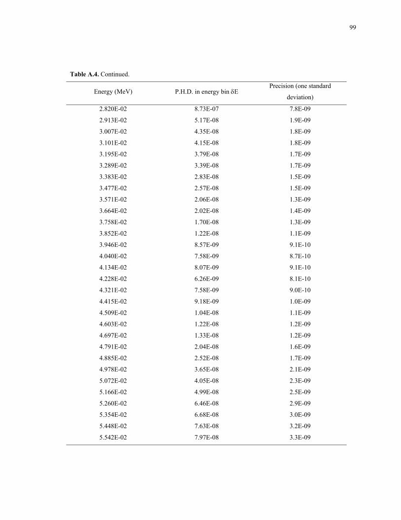
99
Table A.4. Continued.
Energy (MeV) P.H.D. in energy bin δE Precision (one standard
deviation)
2.820E-02 8.73E-07 7.8E-09
2.913E-02 5.17E-08 1.9E-09
3.007E-02 4.35E-08 1.8E-09
3.101E-02 4.15E-08 1.8E-09
3.195E-02 3.79E-08 1.7E-09
3.289E-02 3.39E-08 1.7E-09
3.383E-02 2.83E-08 1.5E-09
3.477E-02 2.57E-08 1.5E-09
3.571E-02 2.06E-08 1.3E-09
3.664E-02 2.02E-08 1.4E-09
3.758E-02 1.70E-08 1.3E-09
3.852E-02 1.22E-08 1.1E-09
3.946E-02 8.57E-09 9.1E-10
4.040E-02 7.58E-09 8.7E-10
4.134E-02 8.07E-09 9.1E-10
4.228E-02 6.26E-09 8.1E-10
4.321E-02 7.58E-09 9.0E-10
4.415E-02 9.18E-09 1.0E-09
4.509E-02 1.04E-08 1.1E-09
4.603E-02 1.22E-08 1.2E-09
4.697E-02 1.33E-08 1.2E-09
4.791E-02 2.04E-08 1.6E-09
4.885E-02 2.52E-08 1.7E-09
4.978E-02 3.65E-08 2.1E-09
5.072E-02 4.05E-08 2.3E-09
5.166E-02 4.99E-08 2.5E-09
5.260E-02 6.46E-08 2.9E-09
5.354E-02 6.68E-08 3.0E-09
5.448E-02 7.63E-08 3.2E-09
5.542E-02 7.97E-08 3.3E-09
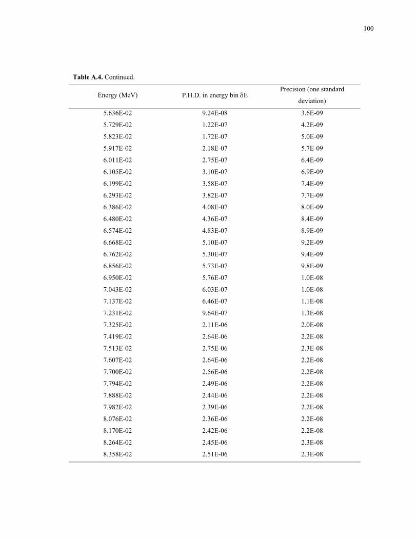
100
Table A.4. Continued.
Energy (MeV) P.H.D. in energy bin δE Precision (one standard
deviation)
5.636E-02 9.24E-08 3.6E-09
5.729E-02 1.22E-07 4.2E-09
5.823E-02 1.72E-07 5.0E-09
5.917E-02 2.18E-07 5.7E-09
6.011E-02 2.75E-07 6.4E-09
6.105E-02 3.10E-07 6.9E-09
6.199E-02 3.58E-07 7.4E-09
6.293E-02 3.82E-07 7.7E-09
6.386E-02 4.08E-07 8.0E-09
6.480E-02 4.36E-07 8.4E-09
6.574E-02 4.83E-07 8.9E-09
6.668E-02 5.10E-07 9.2E-09
6.762E-02 5.30E-07 9.4E-09
6.856E-02 5.73E-07 9.8E-09
6.950E-02 5.76E-07 1.0E-08
7.043E-02 6.03E-07 1.0E-08
7.137E-02 6.46E-07 1.1E-08
7.231E-02 9.64E-07 1.3E-08
7.325E-02 2.11E-06 2.0E-08
7.419E-02 2.64E-06 2.2E-08
7.513E-02 2.75E-06 2.3E-08
7.607E-02 2.64E-06 2.2E-08
7.700E-02 2.56E-06 2.2E-08
7.794E-02 2.49E-06 2.2E-08
7.888E-02 2.44E-06 2.2E-08
7.982E-02 2.39E-06 2.2E-08
8.076E-02 2.36E-06 2.2E-08
8.170E-02 2.42E-06 2.2E-08
8.264E-02 2.45E-06 2.3E-08
8.358E-02 2.51E-06 2.3E-08
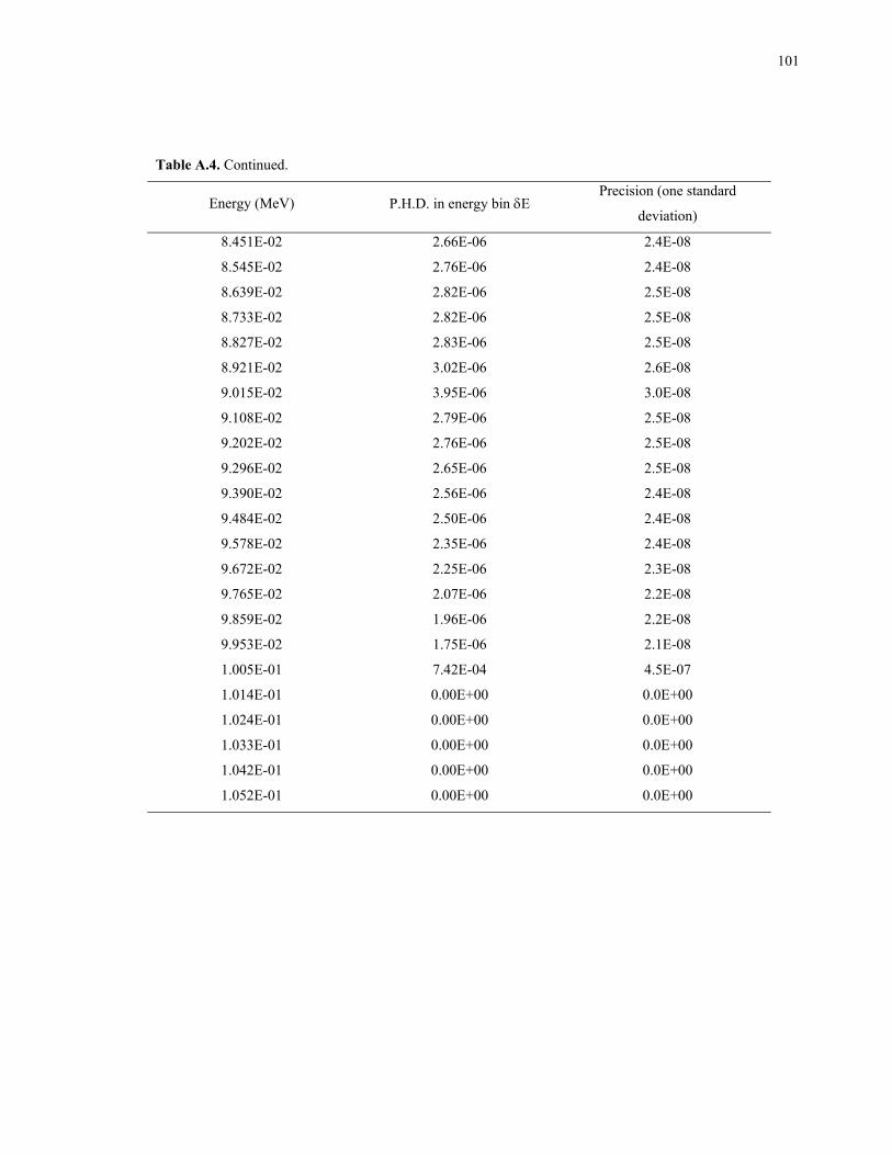
101
Table A.4. Continued.
Energy (MeV) P.H.D. in energy bin δE Precision (one standard
deviation)
8.451E-02 2.66E-06 2.4E-08
8.545E-02 2.76E-06 2.4E-08
8.639E-02 2.82E-06 2.5E-08
8.733E-02 2.82E-06 2.5E-08
8.827E-02 2.83E-06 2.5E-08
8.921E-02 3.02E-06 2.6E-08
9.015E-02 3.95E-06 3.0E-08
9.108E-02 2.79E-06 2.5E-08
9.202E-02 2.76E-06 2.5E-08
9.296E-02 2.65E-06 2.5E-08
9.390E-02 2.56E-06 2.4E-08
9.484E-02 2.50E-06 2.4E-08
9.578E-02 2.35E-06 2.4E-08
9.672E-02 2.25E-06 2.3E-08
9.765E-02 2.07E-06 2.2E-08
9.859E-02 1.96E-06 2.2E-08
9.953E-02 1.75E-06 2.1E-08
1.005E-01 7.42E-04 4.5E-07
1.014E-01 0.00E+00 0.0E+00
1.024E-01 0.00E+00 0.0E+00
1.033E-01 0.00E+00 0.0E+00
1.042E-01 0.00E+00 0.0E+00
1.052E-01 0.00E+00 0.0E+00
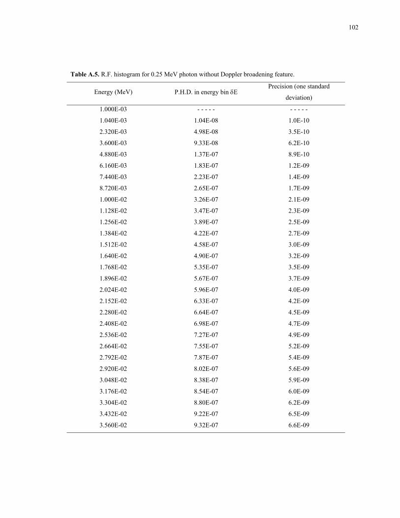
102
Table A.5. R.F. histogram for 0.25 MeV photon without Doppler broadening feature.
Energy (MeV) P.H.D. in energy bin δE Precision (one standard
deviation)
1.000E-03 - - - - - - - - - -
1.040E-03 1.04E-08 1.0E-10
2.320E-03 4.98E-08 3.5E-10
3.600E-03 9.33E-08 6.2E-10
4.880E-03 1.37E-07 8.9E-10
6.160E-03 1.83E-07 1.2E-09
7.440E-03 2.23E-07 1.4E-09
8.720E-03 2.65E-07 1.7E-09
1.000E-02 3.26E-07 2.1E-09
1.128E-02 3.47E-07 2.3E-09
1.256E-02 3.89E-07 2.5E-09
1.384E-02 4.22E-07 2.7E-09
1.512E-02 4.58E-07 3.0E-09
1.640E-02 4.90E-07 3.2E-09
1.768E-02 5.35E-07 3.5E-09
1.896E-02 5.67E-07 3.7E-09
2.024E-02 5.96E-07 4.0E-09
2.152E-02 6.33E-07 4.2E-09
2.280E-02 6.64E-07 4.5E-09
2.408E-02 6.98E-07 4.7E-09
2.536E-02 7.27E-07 4.9E-09
2.664E-02 7.55E-07 5.2E-09
2.792E-02 7.87E-07 5.4E-09
2.920E-02 8.02E-07 5.6E-09
3.048E-02 8.38E-07 5.9E-09
3.176E-02 8.54E-07 6.0E-09
3.304E-02 8.80E-07 6.2E-09
3.432E-02 9.22E-07 6.5E-09
3.560E-02 9.32E-07 6.6E-09
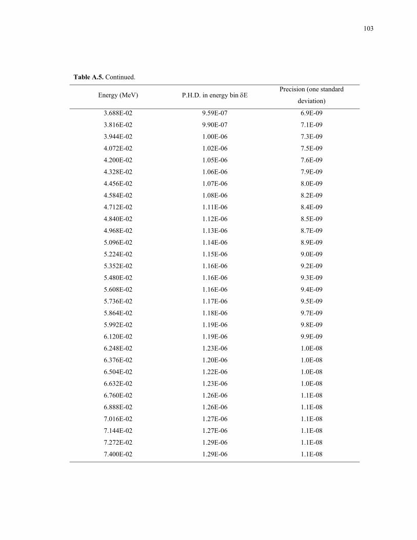
103
Table A.5. Continued.
Energy (MeV) P.H.D. in energy bin δE Precision (one standard
deviation)
3.688E-02 9.59E-07 6.9E-09
3.816E-02 9.90E-07 7.1E-09
3.944E-02 1.00E-06 7.3E-09
4.072E-02 1.02E-06 7.5E-09
4.200E-02 1.05E-06 7.6E-09
4.328E-02 1.06E-06 7.9E-09
4.456E-02 1.07E-06 8.0E-09
4.584E-02 1.08E-06 8.2E-09
4.712E-02 1.11E-06 8.4E-09
4.840E-02 1.12E-06 8.5E-09
4.968E-02 1.13E-06 8.7E-09
5.096E-02 1.14E-06 8.9E-09
5.224E-02 1.15E-06 9.0E-09
5.352E-02 1.16E-06 9.2E-09
5.480E-02 1.16E-06 9.3E-09
5.608E-02 1.16E-06 9.4E-09
5.736E-02 1.17E-06 9.5E-09
5.864E-02 1.18E-06 9.7E-09
5.992E-02 1.19E-06 9.8E-09
6.120E-02 1.19E-06 9.9E-09
6.248E-02 1.23E-06 1.0E-08
6.376E-02 1.20E-06 1.0E-08
6.504E-02 1.22E-06 1.0E-08
6.632E-02 1.23E-06 1.0E-08
6.760E-02 1.26E-06 1.1E-08
6.888E-02 1.26E-06 1.1E-08
7.016E-02 1.27E-06 1.1E-08
7.144E-02 1.27E-06 1.1E-08
7.272E-02 1.29E-06 1.1E-08
7.400E-02 1.29E-06 1.1E-08
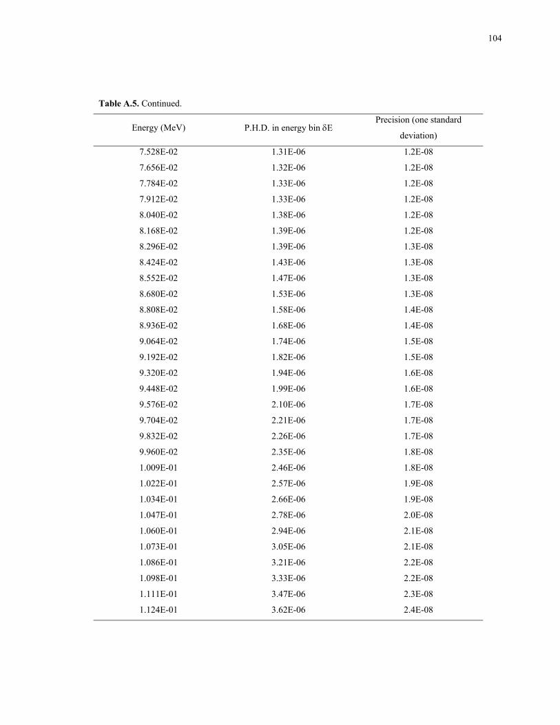
104
Table A.5. Continued.
Energy (MeV) P.H.D. in energy bin δE Precision (one standard
deviation)
7.528E-02 1.31E-06 1.2E-08
7.656E-02 1.32E-06 1.2E-08
7.784E-02 1.33E-06 1.2E-08
7.912E-02 1.33E-06 1.2E-08
8.040E-02 1.38E-06 1.2E-08
8.168E-02 1.39E-06 1.2E-08
8.296E-02 1.39E-06 1.3E-08
8.424E-02 1.43E-06 1.3E-08
8.552E-02 1.47E-06 1.3E-08
8.680E-02 1.53E-06 1.3E-08
8.808E-02 1.58E-06 1.4E-08
8.936E-02 1.68E-06 1.4E-08
9.064E-02 1.74E-06 1.5E-08
9.192E-02 1.82E-06 1.5E-08
9.320E-02 1.94E-06 1.6E-08
9.448E-02 1.99E-06 1.6E-08
9.576E-02 2.10E-06 1.7E-08
9.704E-02 2.21E-06 1.7E-08
9.832E-02 2.26E-06 1.7E-08
9.960E-02 2.35E-06 1.8E-08
1.009E-01 2.46E-06 1.8E-08
1.022E-01 2.57E-06 1.9E-08
1.034E-01 2.66E-06 1.9E-08
1.047E-01 2.78E-06 2.0E-08
1.060E-01 2.94E-06 2.1E-08
1.073E-01 3.05E-06 2.1E-08
1.086E-01 3.21E-06 2.2E-08
1.098E-01 3.33E-06 2.2E-08
1.111E-01 3.47E-06 2.3E-08
1.124E-01 3.62E-06 2.4E-08
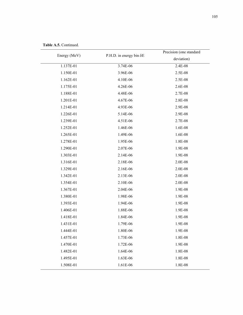
105
Table A.5. Continued.
Energy (MeV) P.H.D. in energy bin δE Precision (one standard
deviation)
1.137E-01 3.74E-06 2.4E-08
1.150E-01 3.96E-06 2.5E-08
1.162E-01 4.10E-06 2.5E-08
1.175E-01 4.26E-06 2.6E-08
1.188E-01 4.48E-06 2.7E-08
1.201E-01 4.67E-06 2.8E-08
1.214E-01 4.93E-06 2.9E-08
1.226E-01 5.14E-06 2.9E-08
1.239E-01 4.51E-06 2.7E-08
1.252E-01 1.46E-06 1.6E-08
1.265E-01 1.49E-06 1.6E-08
1.278E-01 1.95E-06 1.8E-08
1.290E-01 2.07E-06 1.9E-08
1.303E-01 2.14E-06 1.9E-08
1.316E-01 2.18E-06 2.0E-08
1.329E-01 2.16E-06 2.0E-08
1.342E-01 2.13E-06 2.0E-08
1.354E-01 2.10E-06 2.0E-08
1.367E-01 2.04E-06 1.9E-08
1.380E-01 1.98E-06 1.9E-08
1.393E-01 1.94E-06 1.9E-08
1.406E-01 1.88E-06 1.9E-08
1.418E-01 1.84E-06 1.9E-08
1.431E-01 1.79E-06 1.9E-08
1.444E-01 1.80E-06 1.9E-08
1.457E-01 1.73E-06 1.8E-08
1.470E-01 1.72E-06 1.9E-08
1.482E-01 1.64E-06 1.8E-08
1.495E-01 1.63E-06 1.8E-08
1.508E-01 1.61E-06 1.8E-08
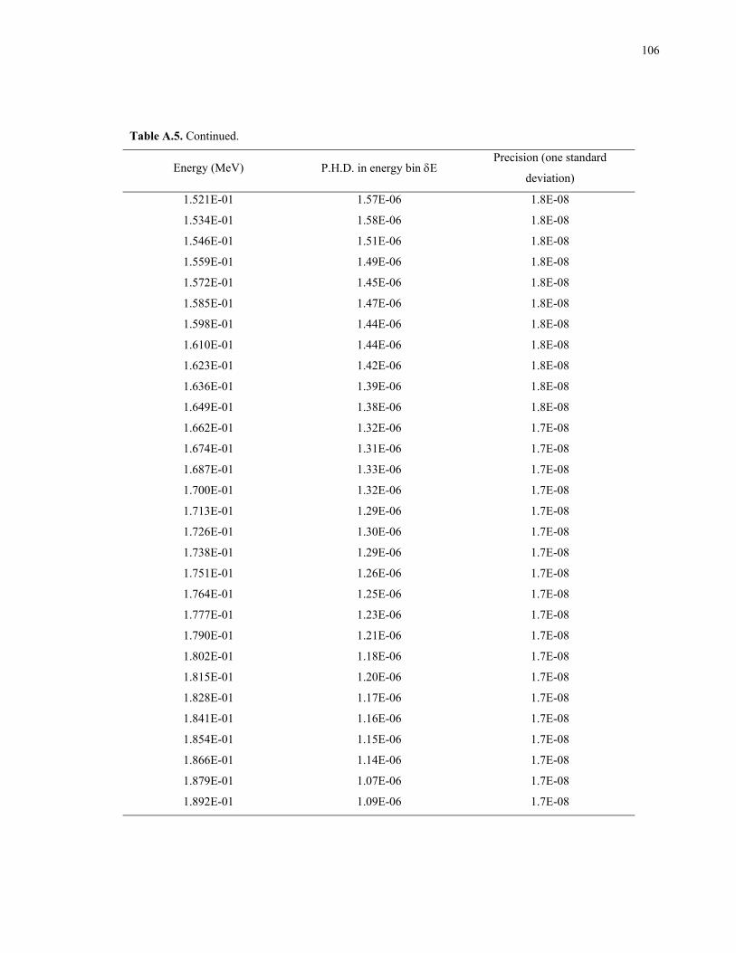
106
Table A.5. Continued.
Energy (MeV) P.H.D. in energy bin δE Precision (one standard
deviation)
1.521E-01 1.57E-06 1.8E-08
1.534E-01 1.58E-06 1.8E-08
1.546E-01 1.51E-06 1.8E-08
1.559E-01 1.49E-06 1.8E-08
1.572E-01 1.45E-06 1.8E-08
1.585E-01 1.47E-06 1.8E-08
1.598E-01 1.44E-06 1.8E-08
1.610E-01 1.44E-06 1.8E-08
1.623E-01 1.42E-06 1.8E-08
1.636E-01 1.39E-06 1.8E-08
1.649E-01 1.38E-06 1.8E-08
1.662E-01 1.32E-06 1.7E-08
1.674E-01 1.31E-06 1.7E-08
1.687E-01 1.33E-06 1.7E-08
1.700E-01 1.32E-06 1.7E-08
1.713E-01 1.29E-06 1.7E-08
1.726E-01 1.30E-06 1.7E-08
1.738E-01 1.29E-06 1.7E-08
1.751E-01 1.26E-06 1.7E-08
1.764E-01 1.25E-06 1.7E-08
1.777E-01 1.23E-06 1.7E-08
1.790E-01 1.21E-06 1.7E-08
1.802E-01 1.18E-06 1.7E-08
1.815E-01 1.20E-06 1.7E-08
1.828E-01 1.17E-06 1.7E-08
1.841E-01 1.16E-06 1.7E-08
1.854E-01 1.15E-06 1.7E-08
1.866E-01 1.14E-06 1.7E-08
1.879E-01 1.07E-06 1.7E-08
1.892E-01 1.09E-06 1.7E-08
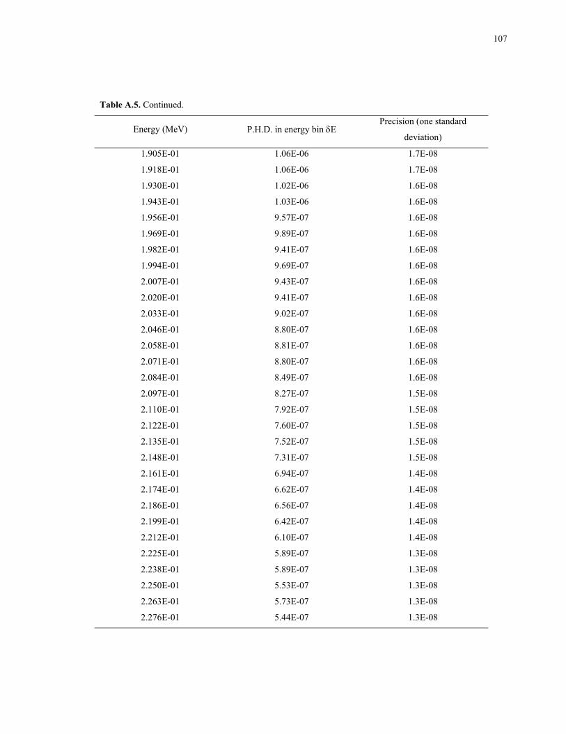
107
Table A.5. Continued.
Energy (MeV) P.H.D. in energy bin δE Precision (one standard
deviation)
1.905E-01 1.06E-06 1.7E-08
1.918E-01 1.06E-06 1.7E-08
1.930E-01 1.02E-06 1.6E-08
1.943E-01 1.03E-06 1.6E-08
1.956E-01 9.57E-07 1.6E-08
1.969E-01 9.89E-07 1.6E-08
1.982E-01 9.41E-07 1.6E-08
1.994E-01 9.69E-07 1.6E-08
2.007E-01 9.43E-07 1.6E-08
2.020E-01 9.41E-07 1.6E-08
2.033E-01 9.02E-07 1.6E-08
2.046E-01 8.80E-07 1.6E-08
2.058E-01 8.81E-07 1.6E-08
2.071E-01 8.80E-07 1.6E-08
2.084E-01 8.49E-07 1.6E-08
2.097E-01 8.27E-07 1.5E-08
2.110E-01 7.92E-07 1.5E-08
2.122E-01 7.60E-07 1.5E-08
2.135E-01 7.52E-07 1.5E-08
2.148E-01 7.31E-07 1.5E-08
2.161E-01 6.94E-07 1.4E-08
2.174E-01 6.62E-07 1.4E-08
2.186E-01 6.56E-07 1.4E-08
2.199E-01 6.42E-07 1.4E-08
2.212E-01 6.10E-07 1.4E-08
2.225E-01 5.89E-07 1.3E-08
2.238E-01 5.89E-07 1.3E-08
2.250E-01 5.53E-07 1.3E-08
2.263E-01 5.73E-07 1.3E-08
2.276E-01 5.44E-07 1.3E-08
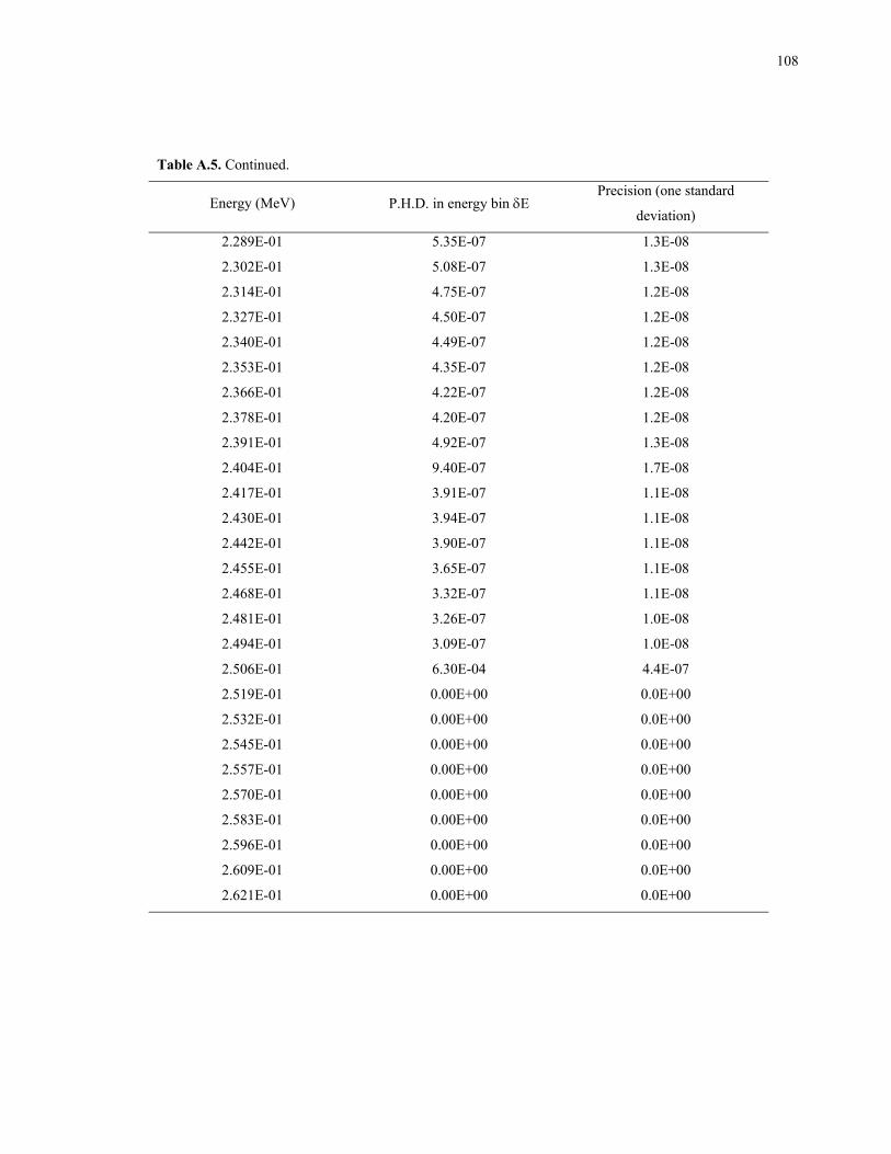
108
Table A.5. Continued.
Energy (MeV) P.H.D. in energy bin δE Precision (one standard
deviation)
2.289E-01 5.35E-07 1.3E-08
2.302E-01 5.08E-07 1.3E-08
2.314E-01 4.75E-07 1.2E-08
2.327E-01 4.50E-07 1.2E-08
2.340E-01 4.49E-07 1.2E-08
2.353E-01 4.35E-07 1.2E-08
2.366E-01 4.22E-07 1.2E-08
2.378E-01 4.20E-07 1.2E-08
2.391E-01 4.92E-07 1.3E-08
2.404E-01 9.40E-07 1.7E-08
2.417E-01 3.91E-07 1.1E-08
2.430E-01 3.94E-07 1.1E-08
2.442E-01 3.90E-07 1.1E-08
2.455E-01 3.65E-07 1.1E-08
2.468E-01 3.32E-07 1.1E-08
2.481E-01 3.26E-07 1.0E-08
2.494E-01 3.09E-07 1.0E-08
2.506E-01 6.30E-04 4.4E-07
2.519E-01 0.00E+00 0.0E+00
2.532E-01 0.00E+00 0.0E+00
2.545E-01 0.00E+00 0.0E+00
2.557E-01 0.00E+00 0.0E+00
2.570E-01 0.00E+00 0.0E+00
2.583E-01 0.00E+00 0.0E+00
2.596E-01 0.00E+00 0.0E+00
2.609E-01 0.00E+00 0.0E+00
2.621E-01 0.00E+00 0.0E+00
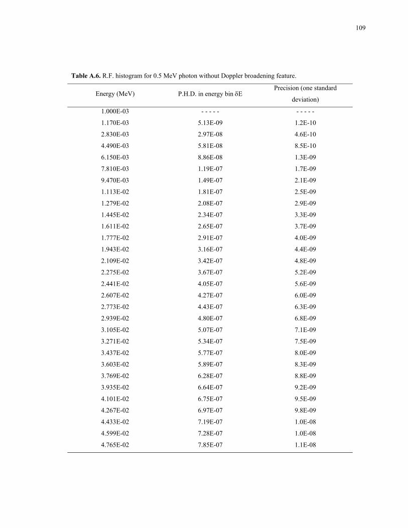
109
Table A.6. R.F. histogram for 0.5 MeV photon without Doppler broadening feature.
Energy (MeV) P.H.D. in energy bin δE Precision (one standard
deviation)
1.000E-03 - - - - - - - - - -
1.170E-03 5.13E-09 1.2E-10
2.830E-03 2.97E-08 4.6E-10
4.490E-03 5.81E-08 8.5E-10
6.150E-03 8.86E-08 1.3E-09
7.810E-03 1.19E-07 1.7E-09
9.470E-03 1.49E-07 2.1E-09
1.113E-02 1.81E-07 2.5E-09
1.279E-02 2.08E-07 2.9E-09
1.445E-02 2.34E-07 3.3E-09
1.611E-02 2.65E-07 3.7E-09
1.777E-02 2.91E-07 4.0E-09
1.943E-02 3.16E-07 4.4E-09
2.109E-02 3.42E-07 4.8E-09
2.275E-02 3.67E-07 5.2E-09
2.441E-02 4.05E-07 5.6E-09
2.607E-02 4.27E-07 6.0E-09
2.773E-02 4.43E-07 6.3E-09
2.939E-02 4.80E-07 6.8E-09
3.105E-02 5.07E-07 7.1E-09
3.271E-02 5.34E-07 7.5E-09
3.437E-02 5.77E-07 8.0E-09
3.603E-02 5.89E-07 8.3E-09
3.769E-02 6.28E-07 8.8E-09
3.935E-02 6.64E-07 9.2E-09
4.101E-02 6.75E-07 9.5E-09
4.267E-02 6.97E-07 9.8E-09
4.433E-02 7.19E-07 1.0E-08
4.599E-02 7.28E-07 1.0E-08
4.765E-02 7.85E-07 1.1E-08
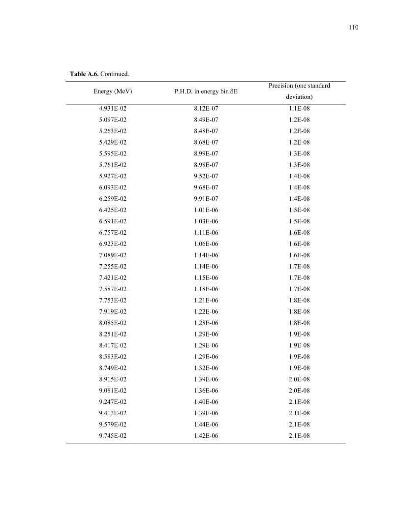
110
Table A.6. Continued.
Energy (MeV) P.H.D. in energy bin δE Precision (one standard
deviation)
4.931E-02 8.12E-07 1.1E-08
5.097E-02 8.49E-07 1.2E-08
5.263E-02 8.48E-07 1.2E-08
5.429E-02 8.68E-07 1.2E-08
5.595E-02 8.99E-07 1.3E-08
5.761E-02 8.98E-07 1.3E-08
5.927E-02 9.52E-07 1.4E-08
6.093E-02 9.68E-07 1.4E-08
6.259E-02 9.91E-07 1.4E-08
6.425E-02 1.01E-06 1.5E-08
6.591E-02 1.03E-06 1.5E-08
6.757E-02 1.11E-06 1.6E-08
6.923E-02 1.06E-06 1.6E-08
7.089E-02 1.14E-06 1.6E-08
7.255E-02 1.14E-06 1.7E-08
7.421E-02 1.15E-06 1.7E-08
7.587E-02 1.18E-06 1.7E-08
7.753E-02 1.21E-06 1.8E-08
7.919E-02 1.22E-06 1.8E-08
8.085E-02 1.28E-06 1.8E-08
8.251E-02 1.29E-06 1.9E-08
8.417E-02 1.29E-06 1.9E-08
8.583E-02 1.29E-06 1.9E-08
8.749E-02 1.32E-06 1.9E-08
8.915E-02 1.39E-06 2.0E-08
9.081E-02 1.36E-06 2.0E-08
9.247E-02 1.40E-06 2.1E-08
9.413E-02 1.39E-06 2.1E-08
9.579E-02 1.44E-06 2.1E-08
9.745E-02 1.42E-06 2.1E-08
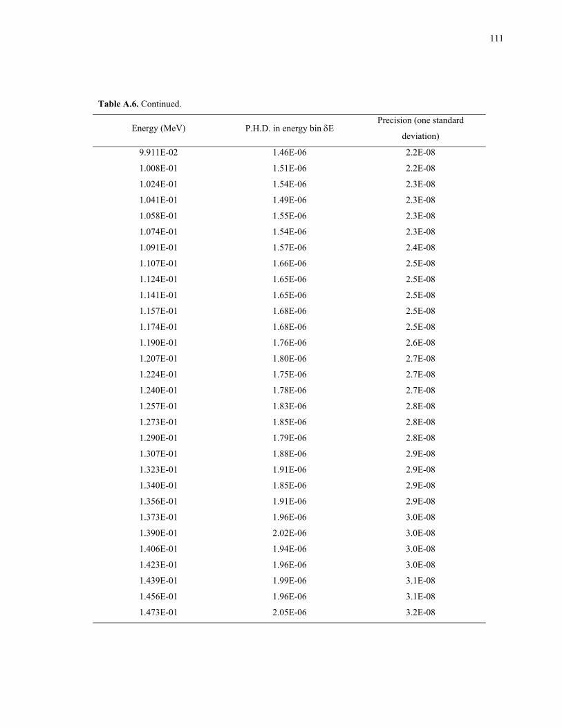
111
Table A.6. Continued.
Energy (MeV) P.H.D. in energy bin δE Precision (one standard
deviation)
9.911E-02 1.46E-06 2.2E-08
1.008E-01 1.51E-06 2.2E-08
1.024E-01 1.54E-06 2.3E-08
1.041E-01 1.49E-06 2.3E-08
1.058E-01 1.55E-06 2.3E-08
1.074E-01 1.54E-06 2.3E-08
1.091E-01 1.57E-06 2.4E-08
1.107E-01 1.66E-06 2.5E-08
1.124E-01 1.65E-06 2.5E-08
1.141E-01 1.65E-06 2.5E-08
1.157E-01 1.68E-06 2.5E-08
1.174E-01 1.68E-06 2.5E-08
1.190E-01 1.76E-06 2.6E-08
1.207E-01 1.80E-06 2.7E-08
1.224E-01 1.75E-06 2.7E-08
1.240E-01 1.78E-06 2.7E-08
1.257E-01 1.83E-06 2.8E-08
1.273E-01 1.85E-06 2.8E-08
1.290E-01 1.79E-06 2.8E-08
1.307E-01 1.88E-06 2.9E-08
1.323E-01 1.91E-06 2.9E-08
1.340E-01 1.85E-06 2.9E-08
1.356E-01 1.91E-06 2.9E-08
1.373E-01 1.96E-06 3.0E-08
1.390E-01 2.02E-06 3.0E-08
1.406E-01 1.94E-06 3.0E-08
1.423E-01 1.96E-06 3.0E-08
1.439E-01 1.99E-06 3.1E-08
1.456E-01 1.96E-06 3.1E-08
1.473E-01 2.05E-06 3.2E-08
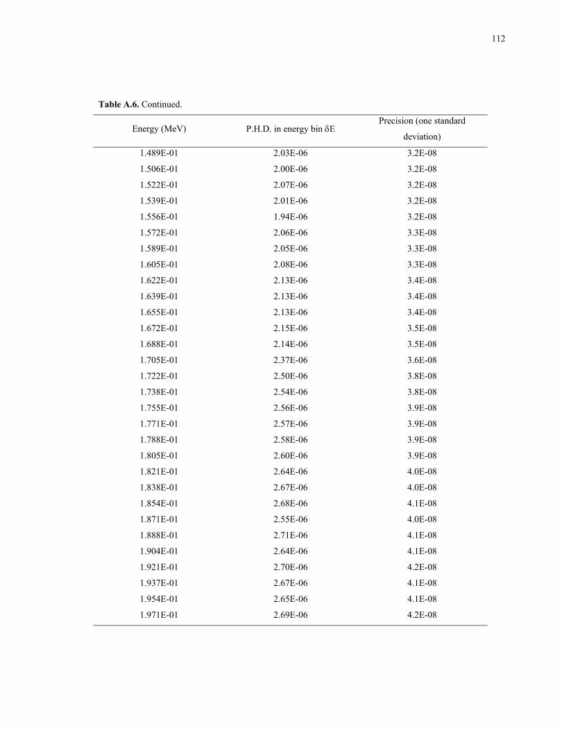
112
Table A.6. Continued.
Energy (MeV) P.H.D. in energy bin δE Precision (one standard
deviation)
1.489E-01 2.03E-06 3.2E-08
1.506E-01 2.00E-06 3.2E-08
1.522E-01 2.07E-06 3.2E-08
1.539E-01 2.01E-06 3.2E-08
1.556E-01 1.94E-06 3.2E-08
1.572E-01 2.06E-06 3.3E-08
1.589E-01 2.05E-06 3.3E-08
1.605E-01 2.08E-06 3.3E-08
1.622E-01 2.13E-06 3.4E-08
1.639E-01 2.13E-06 3.4E-08
1.655E-01 2.13E-06 3.4E-08
1.672E-01 2.15E-06 3.5E-08
1.688E-01 2.14E-06 3.5E-08
1.705E-01 2.37E-06 3.6E-08
1.722E-01 2.50E-06 3.8E-08
1.738E-01 2.54E-06 3.8E-08
1.755E-01 2.56E-06 3.9E-08
1.771E-01 2.57E-06 3.9E-08
1.788E-01 2.58E-06 3.9E-08
1.805E-01 2.60E-06 3.9E-08
1.821E-01 2.64E-06 4.0E-08
1.838E-01 2.67E-06 4.0E-08
1.854E-01 2.68E-06 4.1E-08
1.871E-01 2.55E-06 4.0E-08
1.888E-01 2.71E-06 4.1E-08
1.904E-01 2.64E-06 4.1E-08
1.921E-01 2.70E-06 4.2E-08
1.937E-01 2.67E-06 4.1E-08
1.954E-01 2.65E-06 4.1E-08
1.971E-01 2.69E-06 4.2E-08
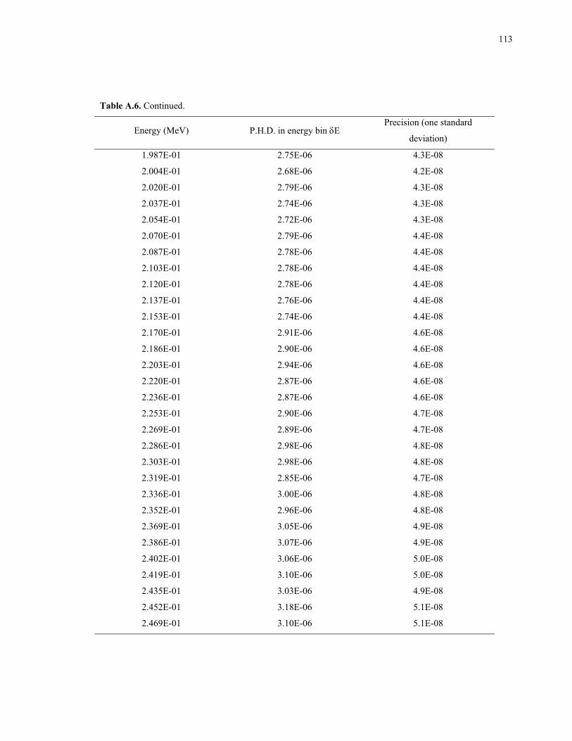
113
Table A.6. Continued.
Energy (MeV) P.H.D. in energy bin δE Precision (one standard
deviation)
1.987E-01 2.75E-06 4.3E-08
2.004E-01 2.68E-06 4.2E-08
2.020E-01 2.79E-06 4.3E-08
2.037E-01 2.74E-06 4.3E-08
2.054E-01 2.72E-06 4.3E-08
2.070E-01 2.79E-06 4.4E-08
2.087E-01 2.78E-06 4.4E-08
2.103E-01 2.78E-06 4.4E-08
2.120E-01 2.78E-06 4.4E-08
2.137E-01 2.76E-06 4.4E-08
2.153E-01 2.74E-06 4.4E-08
2.170E-01 2.91E-06 4.6E-08
2.186E-01 2.90E-06 4.6E-08
2.203E-01 2.94E-06 4.6E-08
2.220E-01 2.87E-06 4.6E-08
2.236E-01 2.87E-06 4.6E-08
2.253E-01 2.90E-06 4.7E-08
2.269E-01 2.89E-06 4.7E-08
2.286E-01 2.98E-06 4.8E-08
2.303E-01 2.98E-06 4.8E-08
2.319E-01 2.85E-06 4.7E-08
2.336E-01 3.00E-06 4.8E-08
2.352E-01 2.96E-06 4.8E-08
2.369E-01 3.05E-06 4.9E-08
2.386E-01 3.07E-06 4.9E-08
2.402E-01 3.06E-06 5.0E-08
2.419E-01 3.10E-06 5.0E-08
2.435E-01 3.03E-06 4.9E-08
2.452E-01 3.18E-06 5.1E-08
2.469E-01 3.10E-06 5.1E-08
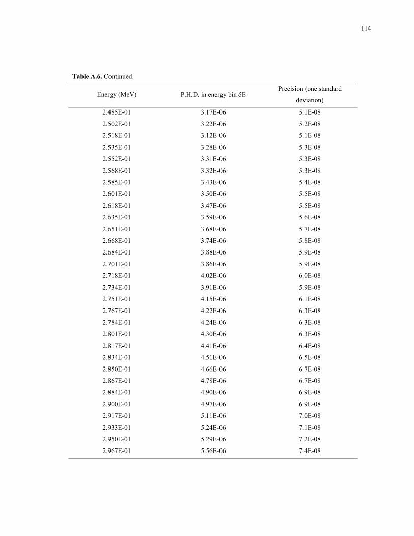
114
Table A.6. Continued.
Energy (MeV) P.H.D. in energy bin δE Precision (one standard
deviation)
2.485E-01 3.17E-06 5.1E-08
2.502E-01 3.22E-06 5.2E-08
2.518E-01 3.12E-06 5.1E-08
2.535E-01 3.28E-06 5.3E-08
2.552E-01 3.31E-06 5.3E-08
2.568E-01 3.32E-06 5.3E-08
2.585E-01 3.43E-06 5.4E-08
2.601E-01 3.50E-06 5.5E-08
2.618E-01 3.47E-06 5.5E-08
2.635E-01 3.59E-06 5.6E-08
2.651E-01 3.68E-06 5.7E-08
2.668E-01 3.74E-06 5.8E-08
2.684E-01 3.88E-06 5.9E-08
2.701E-01 3.86E-06 5.9E-08
2.718E-01 4.02E-06 6.0E-08
2.734E-01 3.91E-06 5.9E-08
2.751E-01 4.15E-06 6.1E-08
2.767E-01 4.22E-06 6.3E-08
2.784E-01 4.24E-06 6.3E-08
2.801E-01 4.30E-06 6.3E-08
2.817E-01 4.41E-06 6.4E-08
2.834E-01 4.51E-06 6.5E-08
2.850E-01 4.66E-06 6.7E-08
2.867E-01 4.78E-06 6.7E-08
2.884E-01 4.90E-06 6.9E-08
2.900E-01 4.97E-06 6.9E-08
2.917E-01 5.11E-06 7.0E-08
2.933E-01 5.24E-06 7.1E-08
2.950E-01 5.29E-06 7.2E-08
2.967E-01 5.56E-06 7.4E-08
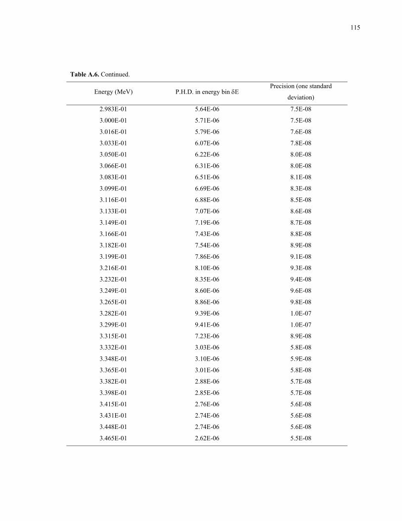
115
Table A.6. Continued.
Energy (MeV) P.H.D. in energy bin δE Precision (one standard
deviation)
2.983E-01 5.64E-06 7.5E-08
3.000E-01 5.71E-06 7.5E-08
3.016E-01 5.79E-06 7.6E-08
3.033E-01 6.07E-06 7.8E-08
3.050E-01 6.22E-06 8.0E-08
3.066E-01 6.31E-06 8.0E-08
3.083E-01 6.51E-06 8.1E-08
3.099E-01 6.69E-06 8.3E-08
3.116E-01 6.88E-06 8.5E-08
3.133E-01 7.07E-06 8.6E-08
3.149E-01 7.19E-06 8.7E-08
3.166E-01 7.43E-06 8.8E-08
3.182E-01 7.54E-06 8.9E-08
3.199E-01 7.86E-06 9.1E-08
3.216E-01 8.10E-06 9.3E-08
3.232E-01 8.35E-06 9.4E-08
3.249E-01 8.60E-06 9.6E-08
3.265E-01 8.86E-06 9.8E-08
3.282E-01 9.39E-06 1.0E-07
3.299E-01 9.41E-06 1.0E-07
3.315E-01 7.23E-06 8.9E-08
3.332E-01 3.03E-06 5.8E-08
3.348E-01 3.10E-06 5.9E-08
3.365E-01 3.01E-06 5.8E-08
3.382E-01 2.88E-06 5.7E-08
3.398E-01 2.85E-06 5.7E-08
3.415E-01 2.76E-06 5.6E-08
3.431E-01 2.74E-06 5.6E-08
3.448E-01 2.74E-06 5.6E-08
3.465E-01 2.62E-06 5.5E-08
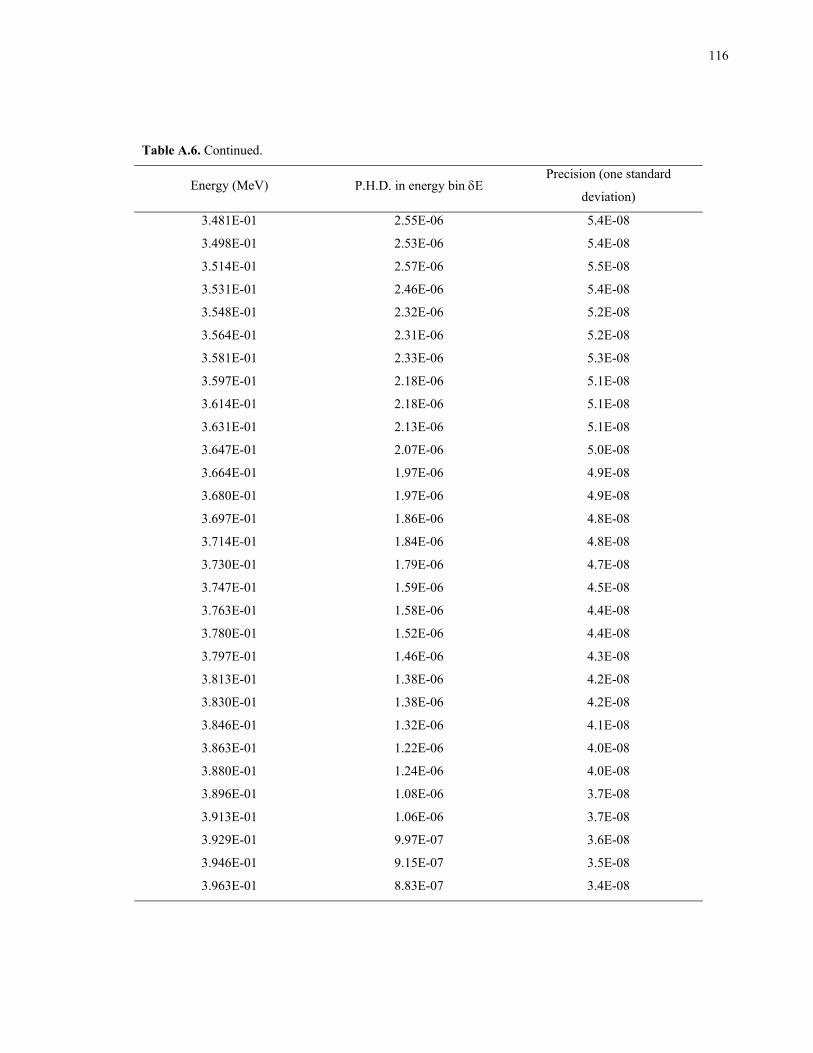
116
Table A.6. Continued.
Energy (MeV) P.H.D. in energy bin δE Precision (one standard
deviation)
3.481E-01 2.55E-06 5.4E-08
3.498E-01 2.53E-06 5.4E-08
3.514E-01 2.57E-06 5.5E-08
3.531E-01 2.46E-06 5.4E-08
3.548E-01 2.32E-06 5.2E-08
3.564E-01 2.31E-06 5.2E-08
3.581E-01 2.33E-06 5.3E-08
3.597E-01 2.18E-06 5.1E-08
3.614E-01 2.18E-06 5.1E-08
3.631E-01 2.13E-06 5.1E-08
3.647E-01 2.07E-06 5.0E-08
3.664E-01 1.97E-06 4.9E-08
3.680E-01 1.97E-06 4.9E-08
3.697E-01 1.86E-06 4.8E-08
3.714E-01 1.84E-06 4.8E-08
3.730E-01 1.79E-06 4.7E-08
3.747E-01 1.59E-06 4.5E-08
3.763E-01 1.58E-06 4.4E-08
3.780E-01 1.52E-06 4.4E-08
3.797E-01 1.46E-06 4.3E-08
3.813E-01 1.38E-06 4.2E-08
3.830E-01 1.38E-06 4.2E-08
3.846E-01 1.32E-06 4.1E-08
3.863E-01 1.22E-06 4.0E-08
3.880E-01 1.24E-06 4.0E-08
3.896E-01 1.08E-06 3.7E-08
3.913E-01 1.06E-06 3.7E-08
3.929E-01 9.97E-07 3.6E-08
3.946E-01 9.15E-07 3.5E-08
3.963E-01 8.83E-07 3.4E-08
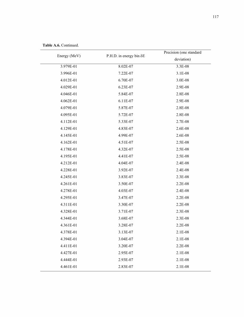
117
Table A.6. Continued.
Energy (MeV) P.H.D. in energy bin δE Precision (one standard
deviation)
3.979E-01 8.02E-07 3.3E-08
3.996E-01 7.22E-07 3.1E-08
4.012E-01 6.70E-07 3.0E-08
4.029E-01 6.23E-07 2.9E-08
4.046E-01 5.84E-07 2.8E-08
4.062E-01 6.11E-07 2.9E-08
4.079E-01 5.87E-07 2.8E-08
4.095E-01 5.72E-07 2.8E-08
4.112E-01 5.33E-07 2.7E-08
4.129E-01 4.83E-07 2.6E-08
4.145E-01 4.99E-07 2.6E-08
4.162E-01 4.51E-07 2.5E-08
4.178E-01 4.32E-07 2.5E-08
4.195E-01 4.41E-07 2.5E-08
4.212E-01 4.04E-07 2.4E-08
4.228E-01 3.92E-07 2.4E-08
4.245E-01 3.83E-07 2.3E-08
4.261E-01 3.50E-07 2.2E-08
4.278E-01 4.03E-07 2.4E-08
4.295E-01 3.47E-07 2.2E-08
4.311E-01 3.30E-07 2.2E-08
4.328E-01 3.71E-07 2.3E-08
4.344E-01 3.68E-07 2.3E-08
4.361E-01 3.28E-07 2.2E-08
4.378E-01 3.13E-07 2.1E-08
4.394E-01 3.04E-07 2.1E-08
4.411E-01 3.20E-07 2.2E-08
4.427E-01 2.95E-07 2.1E-08
4.444E-01 2.93E-07 2.1E-08
4.461E-01 2.83E-07 2.1E-08
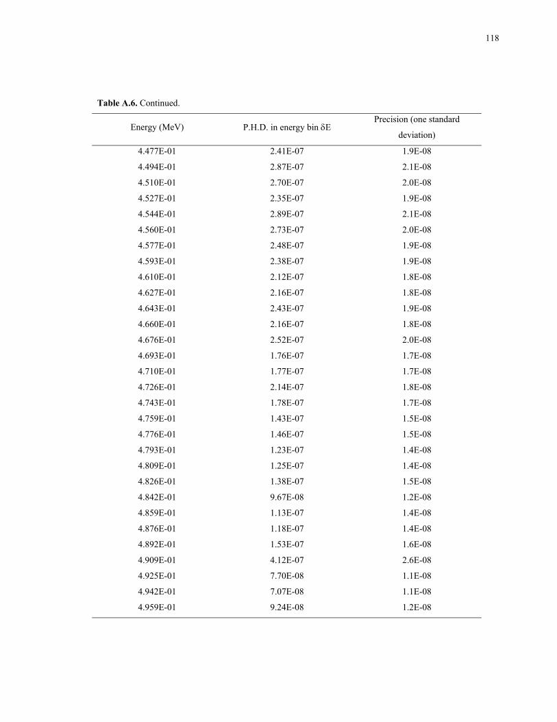
118
Table A.6. Continued.
Energy (MeV) P.H.D. in energy bin δE Precision (one standard
deviation)
4.477E-01 2.41E-07 1.9E-08
4.494E-01 2.87E-07 2.1E-08
4.510E-01 2.70E-07 2.0E-08
4.527E-01 2.35E-07 1.9E-08
4.544E-01 2.89E-07 2.1E-08
4.560E-01 2.73E-07 2.0E-08
4.577E-01 2.48E-07 1.9E-08
4.593E-01 2.38E-07 1.9E-08
4.610E-01 2.12E-07 1.8E-08
4.627E-01 2.16E-07 1.8E-08
4.643E-01 2.43E-07 1.9E-08
4.660E-01 2.16E-07 1.8E-08
4.676E-01 2.52E-07 2.0E-08
4.693E-01 1.76E-07 1.7E-08
4.710E-01 1.77E-07 1.7E-08
4.726E-01 2.14E-07 1.8E-08
4.743E-01 1.78E-07 1.7E-08
4.759E-01 1.43E-07 1.5E-08
4.776E-01 1.46E-07 1.5E-08
4.793E-01 1.23E-07 1.4E-08
4.809E-01 1.25E-07 1.4E-08
4.826E-01 1.38E-07 1.5E-08
4.842E-01 9.67E-08 1.2E-08
4.859E-01 1.13E-07 1.4E-08
4.876E-01 1.18E-07 1.4E-08
4.892E-01 1.53E-07 1.6E-08
4.909E-01 4.12E-07 2.6E-08
4.925E-01 7.70E-08 1.1E-08
4.942E-01 7.07E-08 1.1E-08
4.959E-01 9.24E-08 1.2E-08
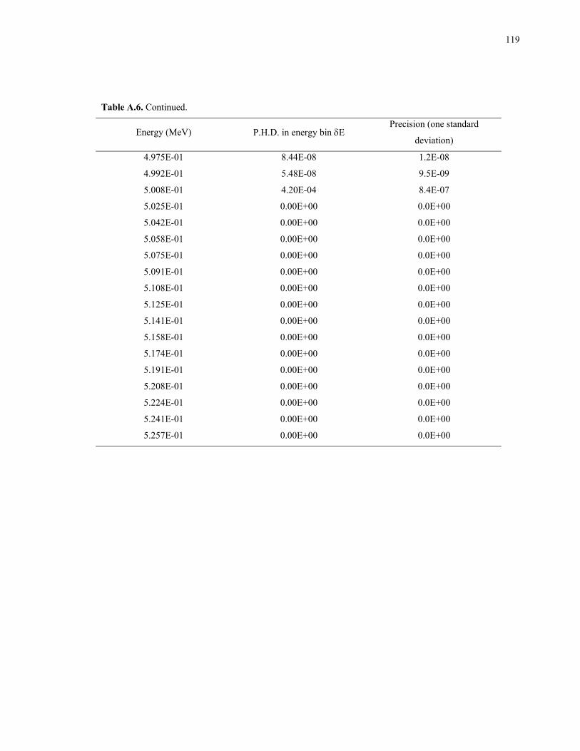
119
Table A.6. Continued.
Energy (MeV) P.H.D. in energy bin δE Precision (one standard
deviation)
4.975E-01 8.44E-08 1.2E-08
4.992E-01 5.48E-08 9.5E-09
5.008E-01 4.20E-04 8.4E-07
5.025E-01 0.00E+00 0.0E+00
5.042E-01 0.00E+00 0.0E+00
5.058E-01 0.00E+00 0.0E+00
5.075E-01 0.00E+00 0.0E+00
5.091E-01 0.00E+00 0.0E+00
5.108E-01 0.00E+00 0.0E+00
5.125E-01 0.00E+00 0.0E+00
5.141E-01 0.00E+00 0.0E+00
5.158E-01 0.00E+00 0.0E+00
5.174E-01 0.00E+00 0.0E+00
5.191E-01 0.00E+00 0.0E+00
5.208E-01 0.00E+00 0.0E+00
5.224E-01 0.00E+00 0.0E+00
5.241E-01 0.00E+00 0.0E+00
5.257E-01 0.00E+00 0.0E+00
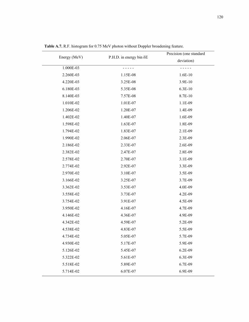
120
Table A.7. R.F. histogram for 0.75 MeV photon without Doppler broadening feature.
Energy (MeV) P.H.D. in energy bin δE Precision (one standard
deviation)
1.000E-03 - - - - - - - - - -
2.260E-03 1.15E-08 1.6E-10
4.220E-03 3.25E-08 3.9E-10
6.180E-03 5.35E-08 6.3E-10
8.140E-03 7.57E-08 8.7E-10
1.010E-02 1.01E-07 1.1E-09
1.206E-02 1.20E-07 1.4E-09
1.402E-02 1.40E-07 1.6E-09
1.598E-02 1.63E-07 1.8E-09
1.794E-02 1.83E-07 2.1E-09
1.990E-02 2.06E-07 2.3E-09
2.186E-02 2.33E-07 2.6E-09
2.382E-02 2.47E-07 2.8E-09
2.578E-02 2.70E-07 3.1E-09
2.774E-02 2.92E-07 3.3E-09
2.970E-02 3.10E-07 3.5E-09
3.166E-02 3.25E-07 3.7E-09
3.362E-02 3.53E-07 4.0E-09
3.558E-02 3.73E-07 4.2E-09
3.754E-02 3.91E-07 4.5E-09
3.950E-02 4.16E-07 4.7E-09
4.146E-02 4.36E-07 4.9E-09
4.342E-02 4.59E-07 5.2E-09
4.538E-02 4.83E-07 5.5E-09
4.734E-02 5.05E-07 5.7E-09
4.930E-02 5.17E-07 5.9E-09
5.126E-02 5.45E-07 6.2E-09
5.322E-02 5.61E-07 6.3E-09
5.518E-02 5.89E-07 6.7E-09
5.714E-02 6.07E-07 6.9E-09
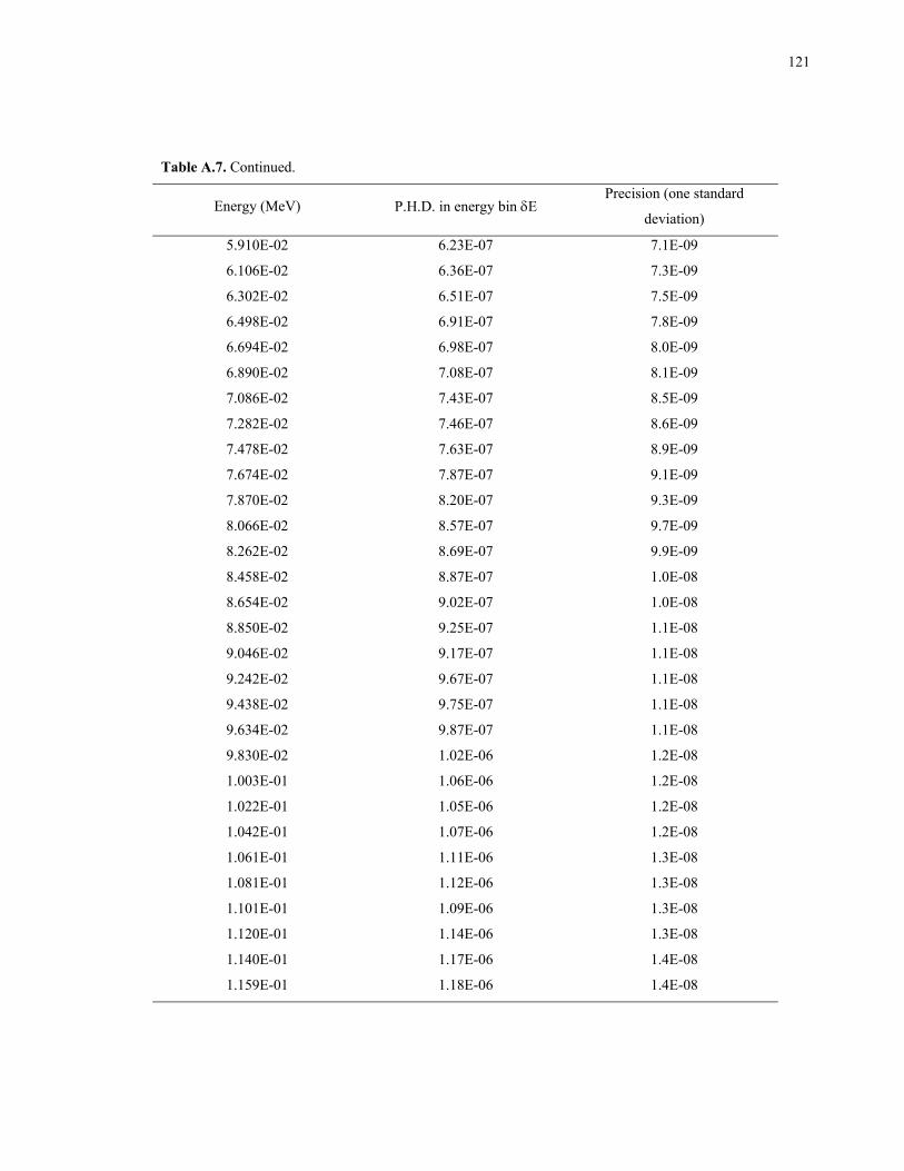
121
Table A.7. Continued.
Energy (MeV) P.H.D. in energy bin δE Precision (one standard
deviation)
5.910E-02 6.23E-07 7.1E-09
6.106E-02 6.36E-07 7.3E-09
6.302E-02 6.51E-07 7.5E-09
6.498E-02 6.91E-07 7.8E-09
6.694E-02 6.98E-07 8.0E-09
6.890E-02 7.08E-07 8.1E-09
7.086E-02 7.43E-07 8.5E-09
7.282E-02 7.46E-07 8.6E-09
7.478E-02 7.63E-07 8.9E-09
7.674E-02 7.87E-07 9.1E-09
7.870E-02 8.20E-07 9.3E-09
8.066E-02 8.57E-07 9.7E-09
8.262E-02 8.69E-07 9.9E-09
8.458E-02 8.87E-07 1.0E-08
8.654E-02 9.02E-07 1.0E-08
8.850E-02 9.25E-07 1.1E-08
9.046E-02 9.17E-07 1.1E-08
9.242E-02 9.67E-07 1.1E-08
9.438E-02 9.75E-07 1.1E-08
9.634E-02 9.87E-07 1.1E-08
9.830E-02 1.02E-06 1.2E-08
1.003E-01 1.06E-06 1.2E-08
1.022E-01 1.05E-06 1.2E-08
1.042E-01 1.07E-06 1.2E-08
1.061E-01 1.11E-06 1.3E-08
1.081E-01 1.12E-06 1.3E-08
1.101E-01 1.09E-06 1.3E-08
1.120E-01 1.14E-06 1.3E-08
1.140E-01 1.17E-06 1.4E-08
1.159E-01 1.18E-06 1.4E-08
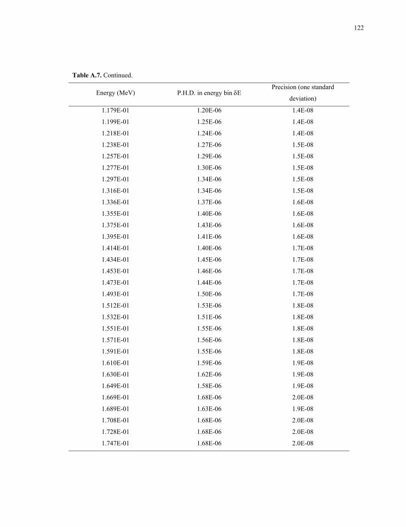
122
Table A.7. Continued.
Energy (MeV) P.H.D. in energy bin δE Precision (one standard
deviation)
1.179E-01 1.20E-06 1.4E-08
1.199E-01 1.25E-06 1.4E-08
1.218E-01 1.24E-06 1.4E-08
1.238E-01 1.27E-06 1.5E-08
1.257E-01 1.29E-06 1.5E-08
1.277E-01 1.30E-06 1.5E-08
1.297E-01 1.34E-06 1.5E-08
1.316E-01 1.34E-06 1.5E-08
1.336E-01 1.37E-06 1.6E-08
1.355E-01 1.40E-06 1.6E-08
1.375E-01 1.43E-06 1.6E-08
1.395E-01 1.41E-06 1.6E-08
1.414E-01 1.40E-06 1.7E-08
1.434E-01 1.45E-06 1.7E-08
1.453E-01 1.46E-06 1.7E-08
1.473E-01 1.44E-06 1.7E-08
1.493E-01 1.50E-06 1.7E-08
1.512E-01 1.53E-06 1.8E-08
1.532E-01 1.51E-06 1.8E-08
1.551E-01 1.55E-06 1.8E-08
1.571E-01 1.56E-06 1.8E-08
1.591E-01 1.55E-06 1.8E-08
1.610E-01 1.59E-06 1.9E-08
1.630E-01 1.62E-06 1.9E-08
1.649E-01 1.58E-06 1.9E-08
1.669E-01 1.68E-06 2.0E-08
1.689E-01 1.63E-06 1.9E-08
1.708E-01 1.68E-06 2.0E-08
1.728E-01 1.68E-06 2.0E-08
1.747E-01 1.68E-06 2.0E-08
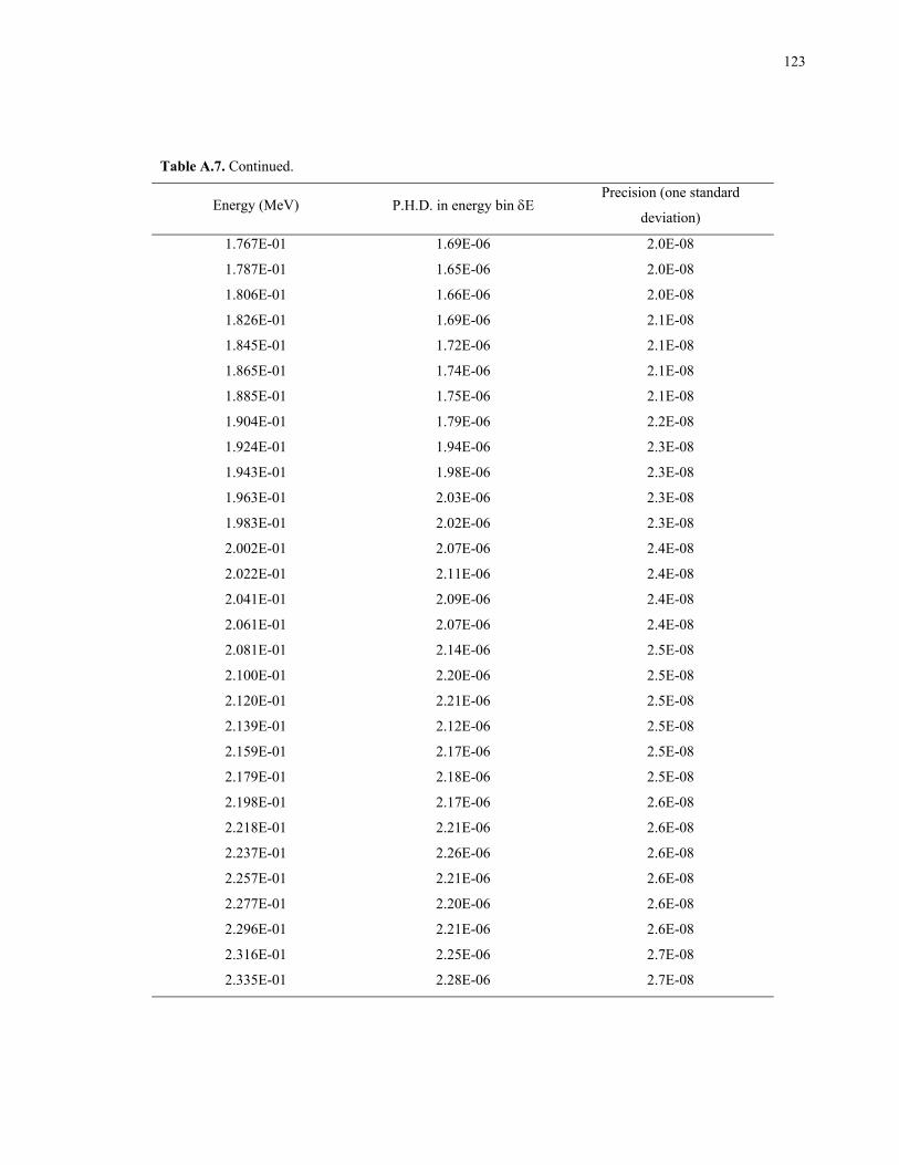
123
Table A.7. Continued.
Energy (MeV) P.H.D. in energy bin δE Precision (one standard
deviation)
1.767E-01 1.69E-06 2.0E-08
1.787E-01 1.65E-06 2.0E-08
1.806E-01 1.66E-06 2.0E-08
1.826E-01 1.69E-06 2.1E-08
1.845E-01 1.72E-06 2.1E-08
1.865E-01 1.74E-06 2.1E-08
1.885E-01 1.75E-06 2.1E-08
1.904E-01 1.79E-06 2.2E-08
1.924E-01 1.94E-06 2.3E-08
1.943E-01 1.98E-06 2.3E-08
1.963E-01 2.03E-06 2.3E-08
1.983E-01 2.02E-06 2.3E-08
2.002E-01 2.07E-06 2.4E-08
2.022E-01 2.11E-06 2.4E-08
2.041E-01 2.09E-06 2.4E-08
2.061E-01 2.07E-06 2.4E-08
2.081E-01 2.14E-06 2.5E-08
2.100E-01 2.20E-06 2.5E-08
2.120E-01 2.21E-06 2.5E-08
2.139E-01 2.12E-06 2.5E-08
2.159E-01 2.17E-06 2.5E-08
2.179E-01 2.18E-06 2.5E-08
2.198E-01 2.17E-06 2.6E-08
2.218E-01 2.21E-06 2.6E-08
2.237E-01 2.26E-06 2.6E-08
2.257E-01 2.21E-06 2.6E-08
2.277E-01 2.20E-06 2.6E-08
2.296E-01 2.21E-06 2.6E-08
2.316E-01 2.25E-06 2.7E-08
2.335E-01 2.28E-06 2.7E-08
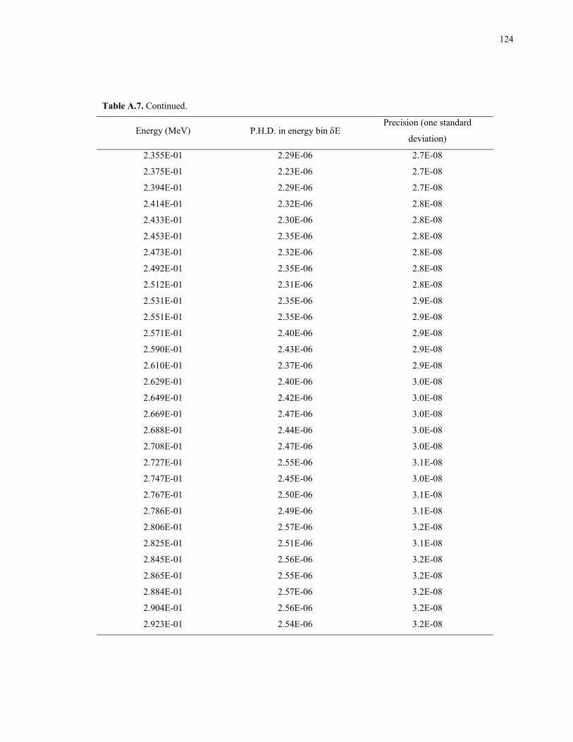
124
Table A.7. Continued.
Energy (MeV) P.H.D. in energy bin δE Precision (one standard
deviation)
2.355E-01 2.29E-06 2.7E-08
2.375E-01 2.23E-06 2.7E-08
2.394E-01 2.29E-06 2.7E-08
2.414E-01 2.32E-06 2.8E-08
2.433E-01 2.30E-06 2.8E-08
2.453E-01 2.35E-06 2.8E-08
2.473E-01 2.32E-06 2.8E-08
2.492E-01 2.35E-06 2.8E-08
2.512E-01 2.31E-06 2.8E-08
2.531E-01 2.35E-06 2.9E-08
2.551E-01 2.35E-06 2.9E-08
2.571E-01 2.40E-06 2.9E-08
2.590E-01 2.43E-06 2.9E-08
2.610E-01 2.37E-06 2.9E-08
2.629E-01 2.40E-06 3.0E-08
2.649E-01 2.42E-06 3.0E-08
2.669E-01 2.47E-06 3.0E-08
2.688E-01 2.44E-06 3.0E-08
2.708E-01 2.47E-06 3.0E-08
2.727E-01 2.55E-06 3.1E-08
2.747E-01 2.45E-06 3.0E-08
2.767E-01 2.50E-06 3.1E-08
2.786E-01 2.49E-06 3.1E-08
2.806E-01 2.57E-06 3.2E-08
2.825E-01 2.51E-06 3.1E-08
2.845E-01 2.56E-06 3.2E-08
2.865E-01 2.55E-06 3.2E-08
2.884E-01 2.57E-06 3.2E-08
2.904E-01 2.56E-06 3.2E-08
2.923E-01 2.54E-06 3.2E-08
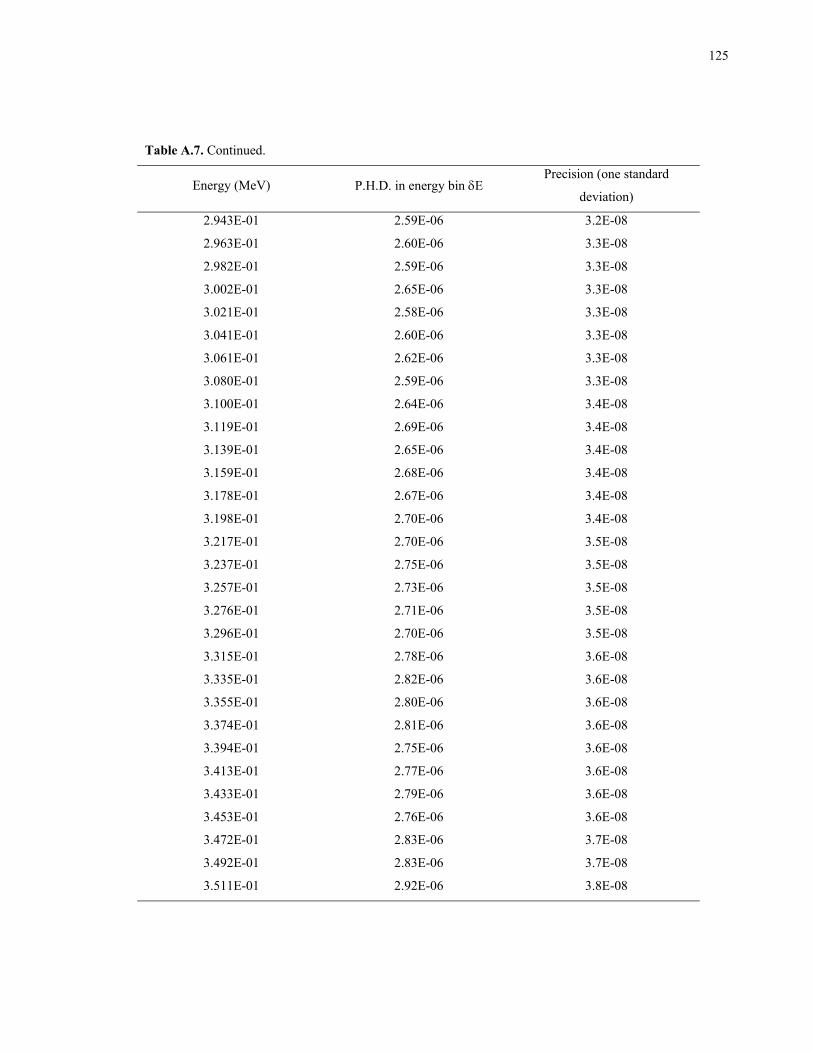
125
Table A.7. Continued.
Energy (MeV) P.H.D. in energy bin δE Precision (one standard
deviation)
2.943E-01 2.59E-06 3.2E-08
2.963E-01 2.60E-06 3.3E-08
2.982E-01 2.59E-06 3.3E-08
3.002E-01 2.65E-06 3.3E-08
3.021E-01 2.58E-06 3.3E-08
3.041E-01 2.60E-06 3.3E-08
3.061E-01 2.62E-06 3.3E-08
3.080E-01 2.59E-06 3.3E-08
3.100E-01 2.64E-06 3.4E-08
3.119E-01 2.69E-06 3.4E-08
3.139E-01 2.65E-06 3.4E-08
3.159E-01 2.68E-06 3.4E-08
3.178E-01 2.67E-06 3.4E-08
3.198E-01 2.70E-06 3.4E-08
3.217E-01 2.70E-06 3.5E-08
3.237E-01 2.75E-06 3.5E-08
3.257E-01 2.73E-06 3.5E-08
3.276E-01 2.71E-06 3.5E-08
3.296E-01 2.70E-06 3.5E-08
3.315E-01 2.78E-06 3.6E-08
3.335E-01 2.82E-06 3.6E-08
3.355E-01 2.80E-06 3.6E-08
3.374E-01 2.81E-06 3.6E-08
3.394E-01 2.75E-06 3.6E-08
3.413E-01 2.77E-06 3.6E-08
3.433E-01 2.79E-06 3.6E-08
3.453E-01 2.76E-06 3.6E-08
3.472E-01 2.83E-06 3.7E-08
3.492E-01 2.83E-06 3.7E-08
3.511E-01 2.92E-06 3.8E-08
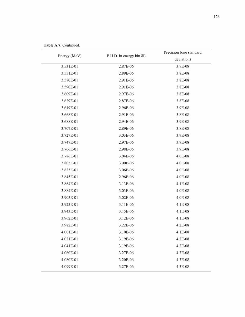
126
Table A.7. Continued.
Energy (MeV) P.H.D. in energy bin δE Precision (one standard
deviation)
3.531E-01 2.87E-06 3.7E-08
3.551E-01 2.89E-06 3.8E-08
3.570E-01 2.91E-06 3.8E-08
3.590E-01 2.91E-06 3.8E-08
3.609E-01 2.97E-06 3.8E-08
3.629E-01 2.87E-06 3.8E-08
3.649E-01 2.96E-06 3.9E-08
3.668E-01 2.91E-06 3.8E-08
3.688E-01 2.94E-06 3.9E-08
3.707E-01 2.89E-06 3.8E-08
3.727E-01 3.03E-06 3.9E-08
3.747E-01 2.97E-06 3.9E-08
3.766E-01 2.98E-06 3.9E-08
3.786E-01 3.04E-06 4.0E-08
3.805E-01 3.00E-06 4.0E-08
3.825E-01 3.06E-06 4.0E-08
3.845E-01 2.96E-06 4.0E-08
3.864E-01 3.13E-06 4.1E-08
3.884E-01 3.03E-06 4.0E-08
3.903E-01 3.02E-06 4.0E-08
3.923E-01 3.11E-06 4.1E-08
3.943E-01 3.15E-06 4.1E-08
3.962E-01 3.12E-06 4.1E-08
3.982E-01 3.22E-06 4.2E-08
4.001E-01 3.10E-06 4.1E-08
4.021E-01 3.19E-06 4.2E-08
4.041E-01 3.19E-06 4.2E-08
4.060E-01 3.27E-06 4.3E-08
4.080E-01 3.20E-06 4.3E-08
4.099E-01 3.27E-06 4.3E-08
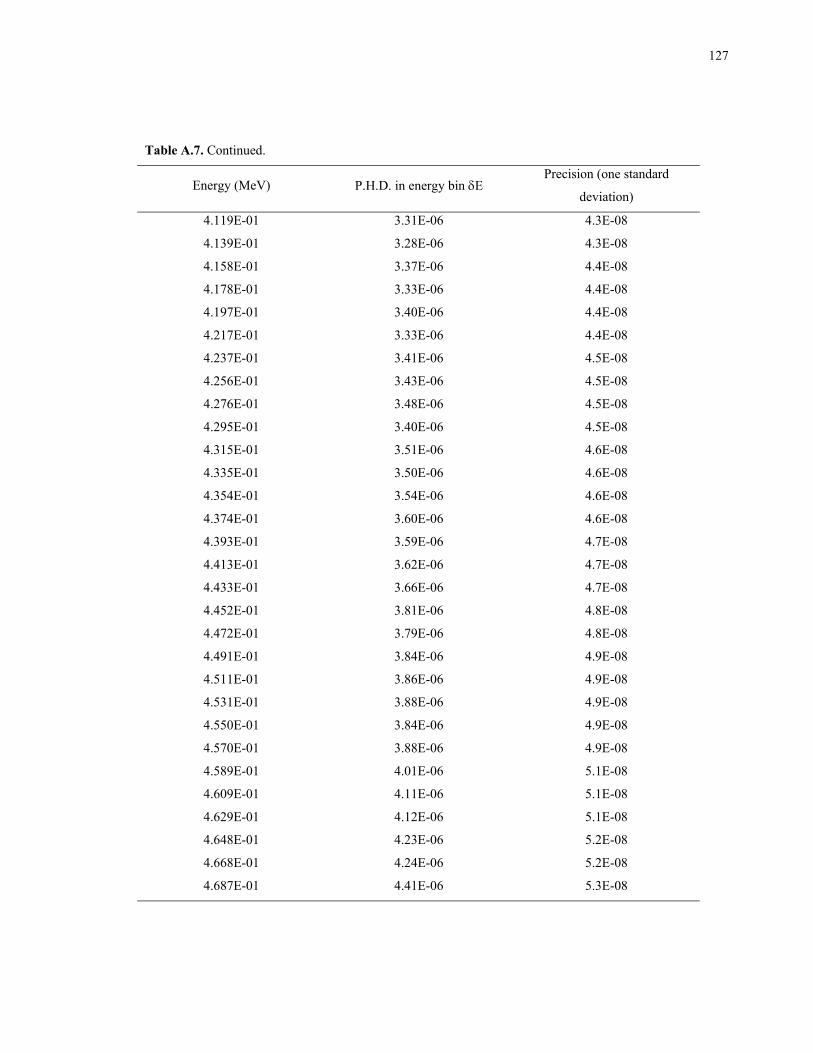
127
Table A.7. Continued.
Energy (MeV) P.H.D. in energy bin δE Precision (one standard
deviation)
4.119E-01 3.31E-06 4.3E-08
4.139E-01 3.28E-06 4.3E-08
4.158E-01 3.37E-06 4.4E-08
4.178E-01 3.33E-06 4.4E-08
4.197E-01 3.40E-06 4.4E-08
4.217E-01 3.33E-06 4.4E-08
4.237E-01 3.41E-06 4.5E-08
4.256E-01 3.43E-06 4.5E-08
4.276E-01 3.48E-06 4.5E-08
4.295E-01 3.40E-06 4.5E-08
4.315E-01 3.51E-06 4.6E-08
4.335E-01 3.50E-06 4.6E-08
4.354E-01 3.54E-06 4.6E-08
4.374E-01 3.60E-06 4.6E-08
4.393E-01 3.59E-06 4.7E-08
4.413E-01 3.62E-06 4.7E-08
4.433E-01 3.66E-06 4.7E-08
4.452E-01 3.81E-06 4.8E-08
4.472E-01 3.79E-06 4.8E-08
4.491E-01 3.84E-06 4.9E-08
4.511E-01 3.86E-06 4.9E-08
4.531E-01 3.88E-06 4.9E-08
4.550E-01 3.84E-06 4.9E-08
4.570E-01 3.88E-06 4.9E-08
4.589E-01 4.01E-06 5.1E-08
4.609E-01 4.11E-06 5.1E-08
4.629E-01 4.12E-06 5.1E-08
4.648E-01 4.23E-06 5.2E-08
4.668E-01 4.24E-06 5.2E-08
4.687E-01 4.41E-06 5.3E-08
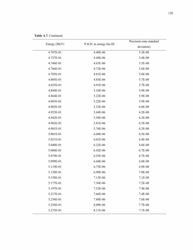
128
Table A.7. Continued.
Energy (MeV) P.H.D. in energy bin δE Precision (one standard
deviation)
4.707E-01 4.40E-06 5.3E-08
4.727E-01 4.48E-06 5.4E-08
4.746E-01 4.63E-06 5.5E-08
4.766E-01 4.72E-06 5.6E-08
4.785E-01 4.81E-06 5.6E-08
4.805E-01 4.83E-06 5.7E-08
4.825E-01 4.91E-06 5.7E-08
4.844E-01 5.16E-06 5.9E-08
4.864E-01 5.22E-06 5.9E-08
4.883E-01 5.22E-06 5.9E-08
4.903E-01 5.32E-06 6.0E-08
4.923E-01 5.64E-06 6.2E-08
4.942E-01 5.58E-06 6.2E-08
4.962E-01 5.81E-06 6.3E-08
4.981E-01 5.76E-06 6.3E-08
5.001E-01 6.04E-06 6.5E-08
5.021E-01 6.01E-06 6.4E-08
5.040E-01 6.22E-06 6.6E-08
5.060E-01 6.42E-06 6.7E-08
5.079E-01 6.55E-06 6.7E-08
5.099E-01 6.64E-06 6.8E-08
5.119E-01 6.75E-06 6.9E-08
5.138E-01 6.90E-06 7.0E-08
5.158E-01 7.13E-06 7.1E-08
5.177E-01 7.36E-06 7.2E-08
5.197E-01 7.52E-06 7.4E-08
5.217E-01 7.66E-06 7.4E-08
5.236E-01 7.88E-06 7.6E-08
5.256E-01 8.09E-06 7.7E-08
5.275E-01 8.11E-06 7.7E-08
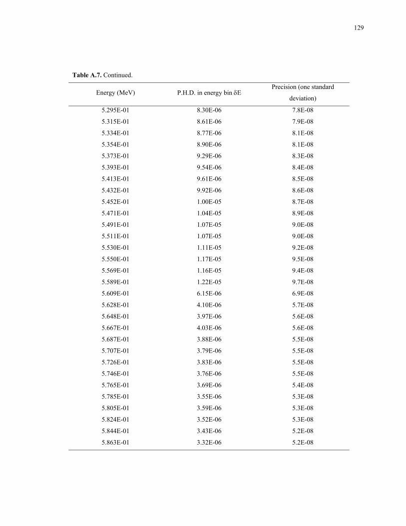
129
Table A.7. Continued.
Energy (MeV) P.H.D. in energy bin δE Precision (one standard
deviation)
5.295E-01 8.30E-06 7.8E-08
5.315E-01 8.61E-06 7.9E-08
5.334E-01 8.77E-06 8.1E-08
5.354E-01 8.90E-06 8.1E-08
5.373E-01 9.29E-06 8.3E-08
5.393E-01 9.54E-06 8.4E-08
5.413E-01 9.61E-06 8.5E-08
5.432E-01 9.92E-06 8.6E-08
5.452E-01 1.00E-05 8.7E-08
5.471E-01 1.04E-05 8.9E-08
5.491E-01 1.07E-05 9.0E-08
5.511E-01 1.07E-05 9.0E-08
5.530E-01 1.11E-05 9.2E-08
5.550E-01 1.17E-05 9.5E-08
5.569E-01 1.16E-05 9.4E-08
5.589E-01 1.22E-05 9.7E-08
5.609E-01 6.15E-06 6.9E-08
5.628E-01 4.10E-06 5.7E-08
5.648E-01 3.97E-06 5.6E-08
5.667E-01 4.03E-06 5.6E-08
5.687E-01 3.88E-06 5.5E-08
5.707E-01 3.79E-06 5.5E-08
5.726E-01 3.83E-06 5.5E-08
5.746E-01 3.76E-06 5.5E-08
5.765E-01 3.69E-06 5.4E-08
5.785E-01 3.55E-06 5.3E-08
5.805E-01 3.59E-06 5.3E-08
5.824E-01 3.52E-06 5.3E-08
5.844E-01 3.43E-06 5.2E-08
5.863E-01 3.32E-06 5.2E-08
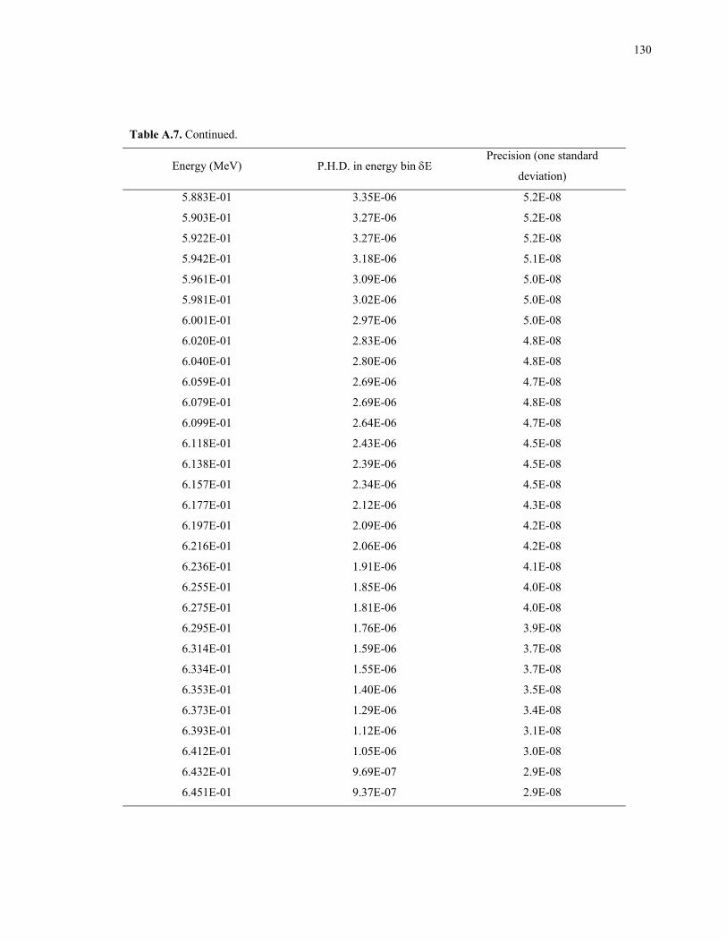
130
Table A.7. Continued.
Energy (MeV) P.H.D. in energy bin δE Precision (one standard
deviation)
5.883E-01 3.35E-06 5.2E-08
5.903E-01 3.27E-06 5.2E-08
5.922E-01 3.27E-06 5.2E-08
5.942E-01 3.18E-06 5.1E-08
5.961E-01 3.09E-06 5.0E-08
5.981E-01 3.02E-06 5.0E-08
6.001E-01 2.97E-06 5.0E-08
6.020E-01 2.83E-06 4.8E-08
6.040E-01 2.80E-06 4.8E-08
6.059E-01 2.69E-06 4.7E-08
6.079E-01 2.69E-06 4.8E-08
6.099E-01 2.64E-06 4.7E-08
6.118E-01 2.43E-06 4.5E-08
6.138E-01 2.39E-06 4.5E-08
6.157E-01 2.34E-06 4.5E-08
6.177E-01 2.12E-06 4.3E-08
6.197E-01 2.09E-06 4.2E-08
6.216E-01 2.06E-06 4.2E-08
6.236E-01 1.91E-06 4.1E-08
6.255E-01 1.85E-06 4.0E-08
6.275E-01 1.81E-06 4.0E-08
6.295E-01 1.76E-06 3.9E-08
6.314E-01 1.59E-06 3.7E-08
6.334E-01 1.55E-06 3.7E-08
6.353E-01 1.40E-06 3.5E-08
6.373E-01 1.29E-06 3.4E-08
6.393E-01 1.12E-06 3.1E-08
6.412E-01 1.05E-06 3.0E-08
6.432E-01 9.69E-07 2.9E-08
6.451E-01 9.37E-07 2.9E-08
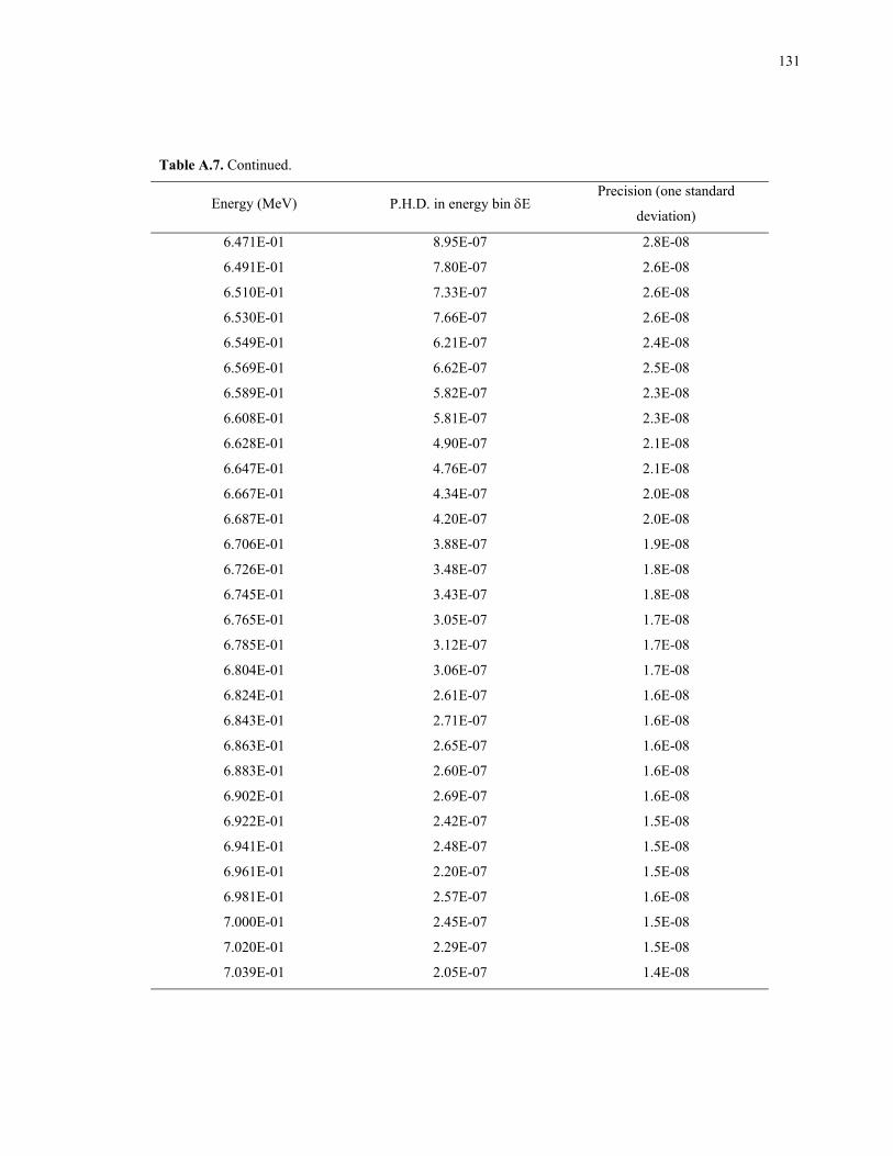
131
Table A.7. Continued.
Energy (MeV) P.H.D. in energy bin δE Precision (one standard
deviation)
6.471E-01 8.95E-07 2.8E-08
6.491E-01 7.80E-07 2.6E-08
6.510E-01 7.33E-07 2.6E-08
6.530E-01 7.66E-07 2.6E-08
6.549E-01 6.21E-07 2.4E-08
6.569E-01 6.62E-07 2.5E-08
6.589E-01 5.82E-07 2.3E-08
6.608E-01 5.81E-07 2.3E-08
6.628E-01 4.90E-07 2.1E-08
6.647E-01 4.76E-07 2.1E-08
6.667E-01 4.34E-07 2.0E-08
6.687E-01 4.20E-07 2.0E-08
6.706E-01 3.88E-07 1.9E-08
6.726E-01 3.48E-07 1.8E-08
6.745E-01 3.43E-07 1.8E-08
6.765E-01 3.05E-07 1.7E-08
6.785E-01 3.12E-07 1.7E-08
6.804E-01 3.06E-07 1.7E-08
6.824E-01 2.61E-07 1.6E-08
6.843E-01 2.71E-07 1.6E-08
6.863E-01 2.65E-07 1.6E-08
6.883E-01 2.60E-07 1.6E-08
6.902E-01 2.69E-07 1.6E-08
6.922E-01 2.42E-07 1.5E-08
6.941E-01 2.48E-07 1.5E-08
6.961E-01 2.20E-07 1.5E-08
6.981E-01 2.57E-07 1.6E-08
7.000E-01 2.45E-07 1.5E-08
7.020E-01 2.29E-07 1.5E-08
7.039E-01 2.05E-07 1.4E-08
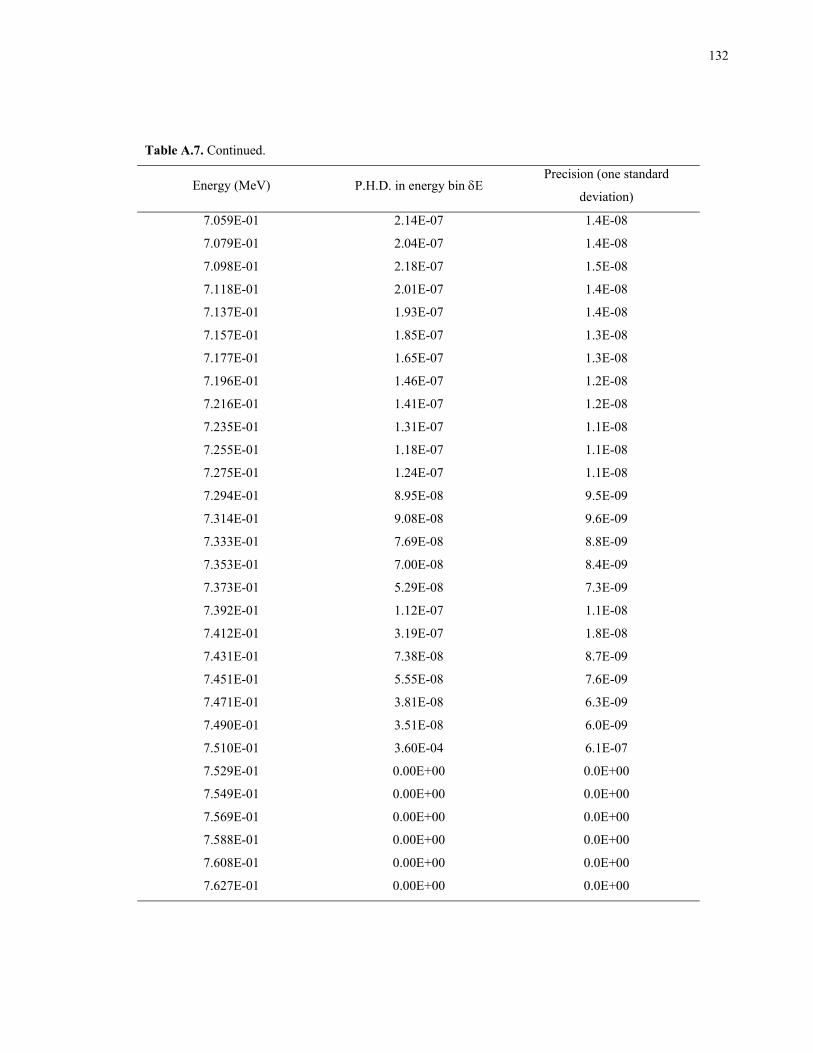
132
Table A.7. Continued.
Energy (MeV) P.H.D. in energy bin δE Precision (one standard
deviation)
7.059E-01 2.14E-07 1.4E-08
7.079E-01 2.04E-07 1.4E-08
7.098E-01 2.18E-07 1.5E-08
7.118E-01 2.01E-07 1.4E-08
7.137E-01 1.93E-07 1.4E-08
7.157E-01 1.85E-07 1.3E-08
7.177E-01 1.65E-07 1.3E-08
7.196E-01 1.46E-07 1.2E-08
7.216E-01 1.41E-07 1.2E-08
7.235E-01 1.31E-07 1.1E-08
7.255E-01 1.18E-07 1.1E-08
7.275E-01 1.24E-07 1.1E-08
7.294E-01 8.95E-08 9.5E-09
7.314E-01 9.08E-08 9.6E-09
7.333E-01 7.69E-08 8.8E-09
7.353E-01 7.00E-08 8.4E-09
7.373E-01 5.29E-08 7.3E-09
7.392E-01 1.12E-07 1.1E-08
7.412E-01 3.19E-07 1.8E-08
7.431E-01 7.38E-08 8.7E-09
7.451E-01 5.55E-08 7.6E-09
7.471E-01 3.81E-08 6.3E-09
7.490E-01 3.51E-08 6.0E-09
7.510E-01 3.60E-04 6.1E-07
7.529E-01 0.00E+00 0.0E+00
7.549E-01 0.00E+00 0.0E+00
7.569E-01 0.00E+00 0.0E+00
7.588E-01 0.00E+00 0.0E+00
7.608E-01 0.00E+00 0.0E+00
7.627E-01 0.00E+00 0.0E+00
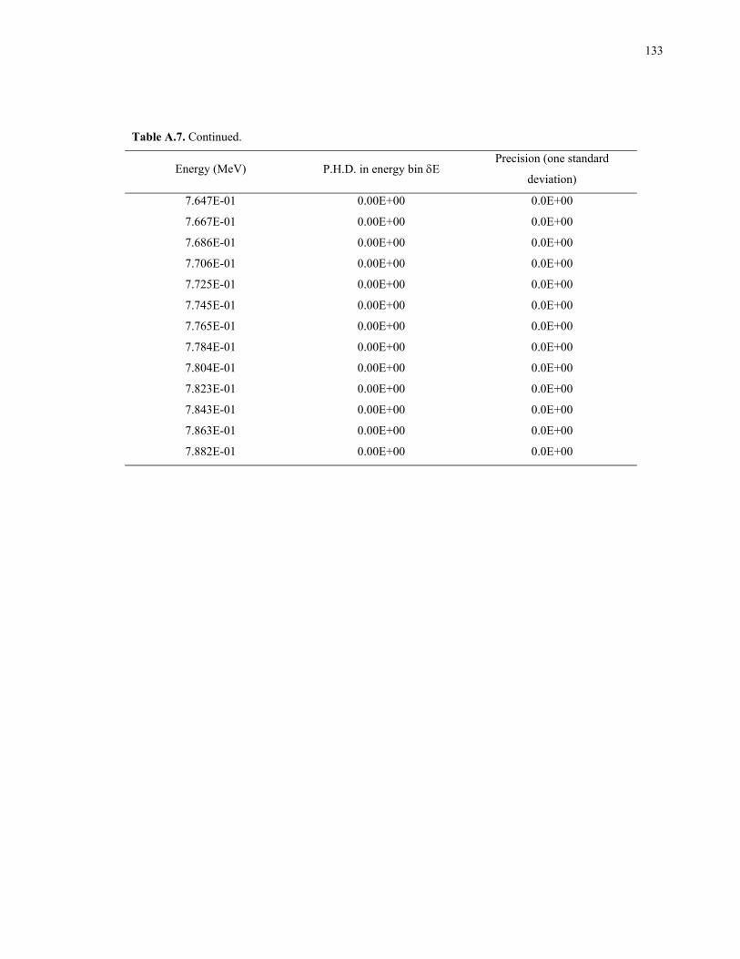
133
Table A.7. Continued.
Energy (MeV) P.H.D. in energy bin δE Precision (one standard
deviation)
7.647E-01 0.00E+00 0.0E+00
7.667E-01 0.00E+00 0.0E+00
7.686E-01 0.00E+00 0.0E+00
7.706E-01 0.00E+00 0.0E+00
7.725E-01 0.00E+00 0.0E+00
7.745E-01 0.00E+00 0.0E+00
7.765E-01 0.00E+00 0.0E+00
7.784E-01 0.00E+00 0.0E+00
7.804E-01 0.00E+00 0.0E+00
7.823E-01 0.00E+00 0.0E+00
7.843E-01 0.00E+00 0.0E+00
7.863E-01 0.00E+00 0.0E+00
7.882E-01 0.00E+00 0.0E+00
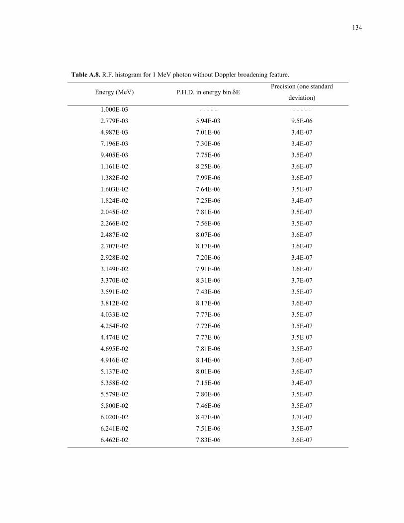
134
Table A.8. R.F. histogram for 1 MeV photon without Doppler broadening feature.
Energy (MeV) P.H.D. in energy bin δE Precision (one standard
deviation)
1.000E-03 - - - - - - - - - -
2.779E-03 5.94E-03 9.5E-06
4.987E-03 7.01E-06 3.4E-07
7.196E-03 7.30E-06 3.4E-07
9.405E-03 7.75E-06 3.5E-07
1.161E-02 8.25E-06 3.6E-07
1.382E-02 7.99E-06 3.6E-07
1.603E-02 7.64E-06 3.5E-07
1.824E-02 7.25E-06 3.4E-07
2.045E-02 7.81E-06 3.5E-07
2.266E-02 7.56E-06 3.5E-07
2.487E-02 8.07E-06 3.6E-07
2.707E-02 8.17E-06 3.6E-07
2.928E-02 7.20E-06 3.4E-07
3.149E-02 7.91E-06 3.6E-07
3.370E-02 8.31E-06 3.7E-07
3.591E-02 7.43E-06 3.5E-07
3.812E-02 8.17E-06 3.6E-07
4.033E-02 7.77E-06 3.5E-07
4.254E-02 7.72E-06 3.5E-07
4.474E-02 7.77E-06 3.5E-07
4.695E-02 7.81E-06 3.5E-07
4.916E-02 8.14E-06 3.6E-07
5.137E-02 8.01E-06 3.6E-07
5.358E-02 7.15E-06 3.4E-07
5.579E-02 7.80E-06 3.5E-07
5.800E-02 7.46E-06 3.5E-07
6.020E-02 8.47E-06 3.7E-07
6.241E-02 7.51E-06 3.5E-07
6.462E-02 7.83E-06 3.6E-07
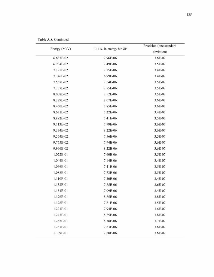
135
Table A.8. Continued.
Energy (MeV) P.H.D. in energy bin δE Precision (one standard
deviation)
6.683E-02 7.96E-06 3.6E-07
6.904E-02 7.49E-06 3.5E-07
7.125E-02 7.15E-06 3.4E-07
7.346E-02 6.99E-06 3.4E-07
7.567E-02 7.54E-06 3.5E-07
7.787E-02 7.75E-06 3.5E-07
8.008E-02 7.52E-06 3.5E-07
8.229E-02 8.07E-06 3.6E-07
8.450E-02 7.85E-06 3.6E-07
8.671E-02 7.22E-06 3.4E-07
8.892E-02 7.41E-06 3.5E-07
9.113E-02 7.99E-06 3.6E-07
9.334E-02 8.22E-06 3.6E-07
9.554E-02 7.56E-06 3.5E-07
9.775E-02 7.94E-06 3.6E-07
9.996E-02 8.22E-06 3.6E-07
1.022E-01 7.60E-06 3.5E-07
1.044E-01 7.14E-06 3.4E-07
1.066E-01 7.41E-06 3.5E-07
1.088E-01 7.73E-06 3.5E-07
1.110E-01 7.30E-06 3.4E-07
1.132E-01 7.85E-06 3.6E-07
1.154E-01 7.09E-06 3.4E-07
1.176E-01 8.85E-06 3.8E-07
1.198E-01 7.81E-06 3.5E-07
1.221E-01 7.94E-06 3.6E-07
1.243E-01 8.25E-06 3.6E-07
1.265E-01 8.38E-06 3.7E-07
1.287E-01 7.83E-06 3.6E-07
1.309E-01 7.88E-06 3.6E-07
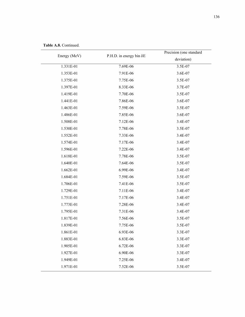
136
Table A.8. Continued.
Energy (MeV) P.H.D. in energy bin δE Precision (one standard
deviation)
1.331E-01 7.69E-06 3.5E-07
1.353E-01 7.91E-06 3.6E-07
1.375E-01 7.75E-06 3.5E-07
1.397E-01 8.33E-06 3.7E-07
1.419E-01 7.70E-06 3.5E-07
1.441E-01 7.86E-06 3.6E-07
1.463E-01 7.59E-06 3.5E-07
1.486E-01 7.85E-06 3.6E-07
1.508E-01 7.12E-06 3.4E-07
1.530E-01 7.78E-06 3.5E-07
1.552E-01 7.33E-06 3.4E-07
1.574E-01 7.17E-06 3.4E-07
1.596E-01 7.22E-06 3.4E-07
1.618E-01 7.78E-06 3.5E-07
1.640E-01 7.64E-06 3.5E-07
1.662E-01 6.99E-06 3.4E-07
1.684E-01 7.59E-06 3.5E-07
1.706E-01 7.41E-06 3.5E-07
1.729E-01 7.11E-06 3.4E-07
1.751E-01 7.17E-06 3.4E-07
1.773E-01 7.28E-06 3.4E-07
1.795E-01 7.31E-06 3.4E-07
1.817E-01 7.56E-06 3.5E-07
1.839E-01 7.75E-06 3.5E-07
1.861E-01 6.93E-06 3.3E-07
1.883E-01 6.83E-06 3.3E-07
1.905E-01 6.72E-06 3.3E-07
1.927E-01 6.90E-06 3.3E-07
1.949E-01 7.25E-06 3.4E-07
1.971E-01 7.52E-06 3.5E-07
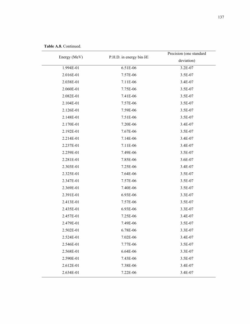
137
Table A.8. Continued.
Energy (MeV) P.H.D. in energy bin δE Precision (one standard
deviation)
1.994E-01 6.51E-06 3.2E-07
2.016E-01 7.57E-06 3.5E-07
2.038E-01 7.11E-06 3.4E-07
2.060E-01 7.75E-06 3.5E-07
2.082E-01 7.41E-06 3.5E-07
2.104E-01 7.57E-06 3.5E-07
2.126E-01 7.59E-06 3.5E-07
2.148E-01 7.51E-06 3.5E-07
2.170E-01 7.20E-06 3.4E-07
2.192E-01 7.67E-06 3.5E-07
2.214E-01 7.14E-06 3.4E-07
2.237E-01 7.11E-06 3.4E-07
2.259E-01 7.49E-06 3.5E-07
2.281E-01 7.85E-06 3.6E-07
2.303E-01 7.25E-06 3.4E-07
2.325E-01 7.64E-06 3.5E-07
2.347E-01 7.57E-06 3.5E-07
2.369E-01 7.40E-06 3.5E-07
2.391E-01 6.93E-06 3.3E-07
2.413E-01 7.57E-06 3.5E-07
2.435E-01 6.93E-06 3.3E-07
2.457E-01 7.25E-06 3.4E-07
2.479E-01 7.49E-06 3.5E-07
2.502E-01 6.78E-06 3.3E-07
2.524E-01 7.02E-06 3.4E-07
2.546E-01 7.77E-06 3.5E-07
2.568E-01 6.64E-06 3.3E-07
2.590E-01 7.43E-06 3.5E-07
2.612E-01 7.38E-06 3.4E-07
2.634E-01 7.22E-06 3.4E-07
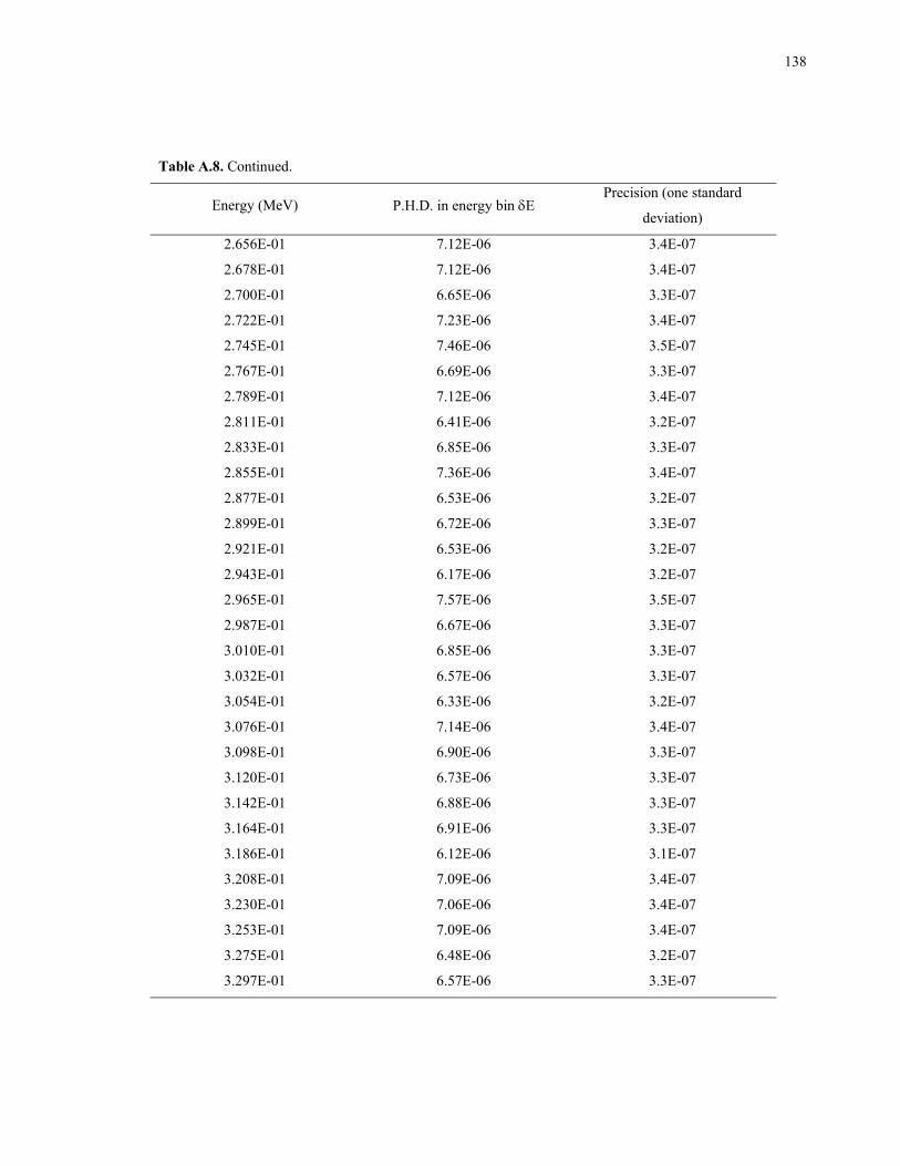
138
Table A.8. Continued.
Energy (MeV) P.H.D. in energy bin δE Precision (one standard
deviation)
2.656E-01 7.12E-06 3.4E-07
2.678E-01 7.12E-06 3.4E-07
2.700E-01 6.65E-06 3.3E-07
2.722E-01 7.23E-06 3.4E-07
2.745E-01 7.46E-06 3.5E-07
2.767E-01 6.69E-06 3.3E-07
2.789E-01 7.12E-06 3.4E-07
2.811E-01 6.41E-06 3.2E-07
2.833E-01 6.85E-06 3.3E-07
2.855E-01 7.36E-06 3.4E-07
2.877E-01 6.53E-06 3.2E-07
2.899E-01 6.72E-06 3.3E-07
2.921E-01 6.53E-06 3.2E-07
2.943E-01 6.17E-06 3.2E-07
2.965E-01 7.57E-06 3.5E-07
2.987E-01 6.67E-06 3.3E-07
3.010E-01 6.85E-06 3.3E-07
3.032E-01 6.57E-06 3.3E-07
3.054E-01 6.33E-06 3.2E-07
3.076E-01 7.14E-06 3.4E-07
3.098E-01 6.90E-06 3.3E-07
3.120E-01 6.73E-06 3.3E-07
3.142E-01 6.88E-06 3.3E-07
3.164E-01 6.91E-06 3.3E-07
3.186E-01 6.12E-06 3.1E-07
3.208E-01 7.09E-06 3.4E-07
3.230E-01 7.06E-06 3.4E-07
3.253E-01 7.09E-06 3.4E-07
3.275E-01 6.48E-06 3.2E-07
3.297E-01 6.57E-06 3.3E-07

139
Table A.8. Continued.
Energy (MeV) P.H.D. in energy bin δE Precision (one standard
deviation)
3.319E-01 6.32E-06 3.2E-07
3.341E-01 6.72E-06 3.3E-07
3.363E-01 6.49E-06 3.2E-07
3.385E-01 6.57E-06 3.3E-07
3.407E-01 5.88E-06 3.1E-07
3.429E-01 6.07E-06 3.1E-07
3.451E-01 6.27E-06 3.2E-07
3.473E-01 6.46E-06 3.2E-07
3.495E-01 6.49E-06 3.2E-07
3.518E-01 6.19E-06 3.2E-07
3.540E-01 6.62E-06 3.3E-07
3.562E-01 6.53E-06 3.2E-07
3.584E-01 6.49E-06 3.2E-07
3.606E-01 6.77E-06 3.3E-07
3.628E-01 6.75E-06 3.3E-07
3.650E-01 6.73E-06 3.3E-07
3.672E-01 5.96E-06 3.1E-07
3.694E-01 6.19E-06 3.2E-07
3.716E-01 6.06E-06 3.1E-07
3.738E-01 6.75E-06 3.3E-07
3.761E-01 6.19E-06 3.2E-07
3.783E-01 5.57E-06 3.0E-07
3.805E-01 5.91E-06 3.1E-07
3.827E-01 6.09E-06 3.1E-07
3.849E-01 6.01E-06 3.1E-07
3.871E-01 6.11E-06 3.1E-07
3.893E-01 5.67E-06 3.0E-07
3.915E-01 6.19E-06 3.2E-07
3.937E-01 6.41E-06 3.2E-07
3.959E-01 6.38E-06 3.2E-07
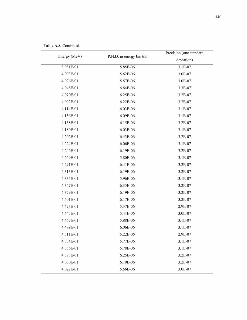
140
Table A.8. Continued.
Energy (MeV) P.H.D. in energy bin δE Precision (one standard
deviation)
3.981E-01 5.85E-06 3.1E-07
4.003E-01 5.62E-06 3.0E-07
4.026E-01 5.57E-06 3.0E-07
4.048E-01 6.64E-06 3.3E-07
4.070E-01 6.25E-06 3.2E-07
4.092E-01 6.22E-06 3.2E-07
4.114E-01 6.03E-06 3.1E-07
4.136E-01 6.09E-06 3.1E-07
4.158E-01 6.15E-06 3.2E-07
4.180E-01 6.03E-06 3.1E-07
4.202E-01 6.43E-06 3.2E-07
4.224E-01 6.06E-06 3.1E-07
4.246E-01 6.19E-06 3.2E-07
4.269E-01 5.80E-06 3.1E-07
4.291E-01 6.41E-06 3.2E-07
4.313E-01 6.19E-06 3.2E-07
4.335E-01 5.96E-06 3.1E-07
4.357E-01 6.35E-06 3.2E-07
4.379E-01 6.19E-06 3.2E-07
4.401E-01 6.17E-06 3.2E-07
4.423E-01 5.37E-06 2.9E-07
4.445E-01 5.41E-06 3.0E-07
4.467E-01 5.88E-06 3.1E-07
4.489E-01 6.06E-06 3.1E-07
4.511E-01 5.22E-06 2.9E-07
4.534E-01 5.77E-06 3.1E-07
4.556E-01 5.78E-06 3.1E-07
4.578E-01 6.25E-06 3.2E-07
4.600E-01 6.19E-06 3.2E-07
4.622E-01 5.56E-06 3.0E-07
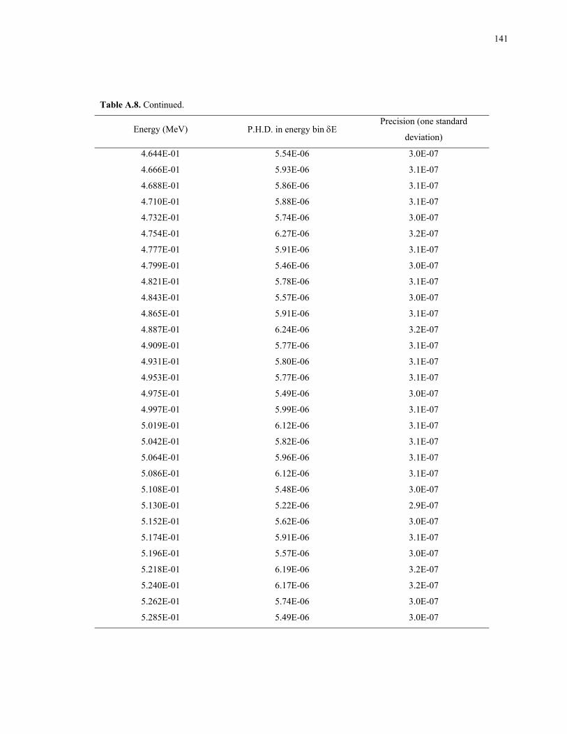
141
Table A.8. Continued.
Energy (MeV) P.H.D. in energy bin δE Precision (one standard
deviation)
4.644E-01 5.54E-06 3.0E-07
4.666E-01 5.93E-06 3.1E-07
4.688E-01 5.86E-06 3.1E-07
4.710E-01 5.88E-06 3.1E-07
4.732E-01 5.74E-06 3.0E-07
4.754E-01 6.27E-06 3.2E-07
4.777E-01 5.91E-06 3.1E-07
4.799E-01 5.46E-06 3.0E-07
4.821E-01 5.78E-06 3.1E-07
4.843E-01 5.57E-06 3.0E-07
4.865E-01 5.91E-06 3.1E-07
4.887E-01 6.24E-06 3.2E-07
4.909E-01 5.77E-06 3.1E-07
4.931E-01 5.80E-06 3.1E-07
4.953E-01 5.77E-06 3.1E-07
4.975E-01 5.49E-06 3.0E-07
4.997E-01 5.99E-06 3.1E-07
5.019E-01 6.12E-06 3.1E-07
5.042E-01 5.82E-06 3.1E-07
5.064E-01 5.96E-06 3.1E-07
5.086E-01 6.12E-06 3.1E-07
5.108E-01 5.48E-06 3.0E-07
5.130E-01 5.22E-06 2.9E-07
5.152E-01 5.62E-06 3.0E-07
5.174E-01 5.91E-06 3.1E-07
5.196E-01 5.57E-06 3.0E-07
5.218E-01 6.19E-06 3.2E-07
5.240E-01 6.17E-06 3.2E-07
5.262E-01 5.74E-06 3.0E-07
5.285E-01 5.49E-06 3.0E-07
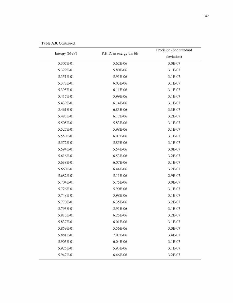
142
Table A.8. Continued.
Energy (MeV) P.H.D. in energy bin δE Precision (one standard
deviation)
5.307E-01 5.62E-06 3.0E-07
5.329E-01 5.80E-06 3.1E-07
5.351E-01 5.91E-06 3.1E-07
5.373E-01 6.03E-06 3.1E-07
5.395E-01 6.11E-06 3.1E-07
5.417E-01 5.99E-06 3.1E-07
5.439E-01 6.14E-06 3.1E-07
5.461E-01 6.83E-06 3.3E-07
5.483E-01 6.17E-06 3.2E-07
5.505E-01 5.83E-06 3.1E-07
5.527E-01 5.98E-06 3.1E-07
5.550E-01 6.07E-06 3.1E-07
5.572E-01 5.85E-06 3.1E-07
5.594E-01 5.54E-06 3.0E-07
5.616E-01 6.53E-06 3.2E-07
5.638E-01 6.07E-06 3.1E-07
5.660E-01 6.44E-06 3.2E-07
5.682E-01 5.11E-06 2.9E-07
5.704E-01 5.75E-06 3.0E-07
5.726E-01 5.90E-06 3.1E-07
5.748E-01 5.98E-06 3.1E-07
5.770E-01 6.35E-06 3.2E-07
5.793E-01 5.91E-06 3.1E-07
5.815E-01 6.25E-06 3.2E-07
5.837E-01 6.01E-06 3.1E-07
5.859E-01 5.56E-06 3.0E-07
5.881E-01 7.07E-06 3.4E-07
5.903E-01 6.04E-06 3.1E-07
5.925E-01 5.93E-06 3.1E-07
5.947E-01 6.46E-06 3.2E-07
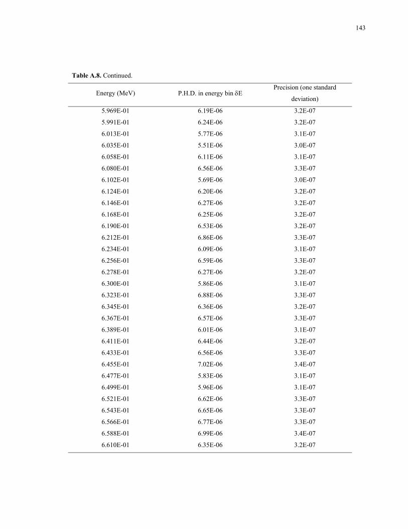
143
Table A.8. Continued.
Energy (MeV) P.H.D. in energy bin δE Precision (one standard
deviation)
5.969E-01 6.19E-06 3.2E-07
5.991E-01 6.24E-06 3.2E-07
6.013E-01 5.77E-06 3.1E-07
6.035E-01 5.51E-06 3.0E-07
6.058E-01 6.11E-06 3.1E-07
6.080E-01 6.56E-06 3.3E-07
6.102E-01 5.69E-06 3.0E-07
6.124E-01 6.20E-06 3.2E-07
6.146E-01 6.27E-06 3.2E-07
6.168E-01 6.25E-06 3.2E-07
6.190E-01 6.53E-06 3.2E-07
6.212E-01 6.86E-06 3.3E-07
6.234E-01 6.09E-06 3.1E-07
6.256E-01 6.59E-06 3.3E-07
6.278E-01 6.27E-06 3.2E-07
6.300E-01 5.86E-06 3.1E-07
6.323E-01 6.88E-06 3.3E-07
6.345E-01 6.36E-06 3.2E-07
6.367E-01 6.57E-06 3.3E-07
6.389E-01 6.01E-06 3.1E-07
6.411E-01 6.44E-06 3.2E-07
6.433E-01 6.56E-06 3.3E-07
6.455E-01 7.02E-06 3.4E-07
6.477E-01 5.83E-06 3.1E-07
6.499E-01 5.96E-06 3.1E-07
6.521E-01 6.62E-06 3.3E-07
6.543E-01 6.65E-06 3.3E-07
6.566E-01 6.77E-06 3.3E-07
6.588E-01 6.99E-06 3.4E-07
6.610E-01 6.35E-06 3.2E-07
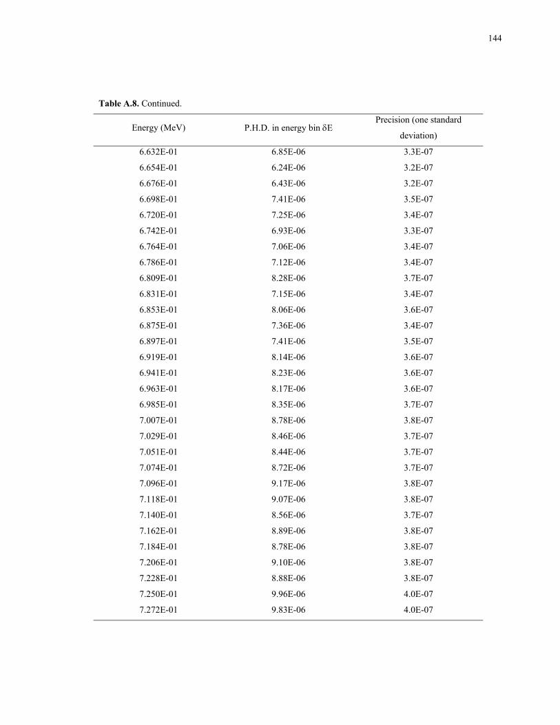
144
Table A.8. Continued.
Energy (MeV) P.H.D. in energy bin δE Precision (one standard
deviation)
6.632E-01 6.85E-06 3.3E-07
6.654E-01 6.24E-06 3.2E-07
6.676E-01 6.43E-06 3.2E-07
6.698E-01 7.41E-06 3.5E-07
6.720E-01 7.25E-06 3.4E-07
6.742E-01 6.93E-06 3.3E-07
6.764E-01 7.06E-06 3.4E-07
6.786E-01 7.12E-06 3.4E-07
6.809E-01 8.28E-06 3.7E-07
6.831E-01 7.15E-06 3.4E-07
6.853E-01 8.06E-06 3.6E-07
6.875E-01 7.36E-06 3.4E-07
6.897E-01 7.41E-06 3.5E-07
6.919E-01 8.14E-06 3.6E-07
6.941E-01 8.23E-06 3.6E-07
6.963E-01 8.17E-06 3.6E-07
6.985E-01 8.35E-06 3.7E-07
7.007E-01 8.78E-06 3.8E-07
7.029E-01 8.46E-06 3.7E-07
7.051E-01 8.44E-06 3.7E-07
7.074E-01 8.72E-06 3.7E-07
7.096E-01 9.17E-06 3.8E-07
7.118E-01 9.07E-06 3.8E-07
7.140E-01 8.56E-06 3.7E-07
7.162E-01 8.89E-06 3.8E-07
7.184E-01 8.78E-06 3.8E-07
7.206E-01 9.10E-06 3.8E-07
7.228E-01 8.88E-06 3.8E-07
7.250E-01 9.96E-06 4.0E-07
7.272E-01 9.83E-06 4.0E-07

145
Table A.8. Continued.
Energy (MeV) P.H.D. in energy bin δE Precision (one standard
deviation)
7.294E-01 1.07E-05 4.2E-07
7.316E-01 1.03E-05 4.1E-07
7.339E-01 9.68E-06 4.0E-07
7.361E-01 1.03E-05 4.1E-07
7.383E-01 1.08E-05 4.2E-07
7.405E-01 1.04E-05 4.1E-07
7.427E-01 1.13E-05 4.3E-07
7.449E-01 1.11E-05 4.2E-07
7.471E-01 1.07E-05 4.2E-07
7.493E-01 1.22E-05 4.4E-07
7.515E-01 1.20E-05 4.4E-07
7.537E-01 1.17E-05 4.3E-07
7.559E-01 1.34E-05 4.6E-07
7.582E-01 1.29E-05 4.6E-07
7.604E-01 1.32E-05 4.6E-07
7.626E-01 1.30E-05 4.6E-07
7.648E-01 1.38E-05 4.7E-07
7.670E-01 1.34E-05 4.7E-07
7.692E-01 1.34E-05 4.6E-07
7.714E-01 1.41E-05 4.8E-07
7.736E-01 1.56E-05 5.0E-07
7.758E-01 1.47E-05 4.9E-07
7.780E-01 1.52E-05 5.0E-07
7.802E-01 1.53E-05 5.0E-07
7.824E-01 1.59E-05 5.1E-07
7.847E-01 1.72E-05 5.3E-07
7.869E-01 1.70E-05 5.2E-07
7.891E-01 1.69E-05 5.2E-07
7.913E-01 1.67E-05 5.2E-07
7.935E-01 1.76E-05 5.3E-07

146
Table A.8. Continued.
Energy (MeV) P.H.D. in energy bin δE Precision (one standard
deviation)
7.957E-01 1.79E-05 5.4E-07
7.979E-01 1.01E-05 4.0E-07
8.001E-01 6.72E-06 3.3E-07
8.023E-01 5.85E-06 3.1E-07
8.045E-01 5.82E-06 3.1E-07
8.067E-01 5.62E-06 3.0E-07
8.090E-01 5.66E-06 3.0E-07
8.112E-01 5.99E-06 3.1E-07
8.134E-01 5.33E-06 2.9E-07
8.156E-01 5.64E-06 3.0E-07
8.178E-01 5.61E-06 3.0E-07
8.200E-01 5.67E-06 3.0E-07
8.222E-01 5.12E-06 2.9E-07
8.244E-01 5.35E-06 2.9E-07
8.266E-01 4.85E-06 2.8E-07
8.288E-01 5.32E-06 2.9E-07
8.310E-01 5.20E-06 2.9E-07
8.332E-01 5.51E-06 3.0E-07
8.355E-01 4.70E-06 2.8E-07
8.377E-01 4.66E-06 2.7E-07
8.399E-01 4.43E-06 2.7E-07
8.421E-01 4.35E-06 2.6E-07
8.443E-01 4.43E-06 2.7E-07
8.465E-01 4.37E-06 2.7E-07
8.487E-01 4.19E-06 2.6E-07
8.509E-01 3.71E-06 2.4E-07
8.531E-01 3.51E-06 2.4E-07
8.553E-01 3.37E-06 2.3E-07
8.575E-01 3.54E-06 2.4E-07
8.598E-01 3.56E-06 2.4E-07
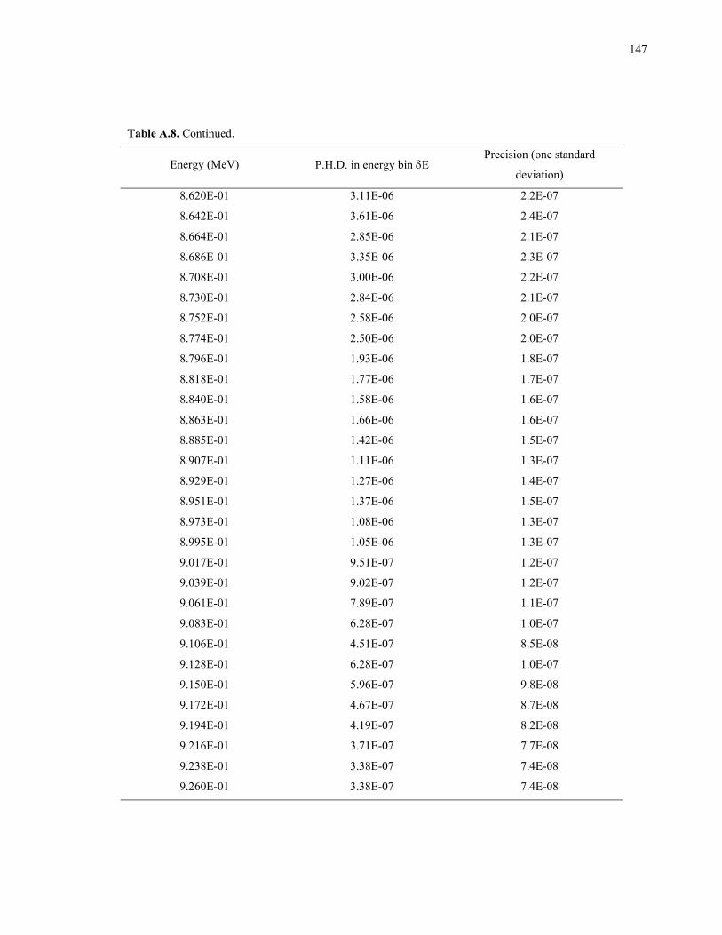
147
Table A.8. Continued.
Energy (MeV) P.H.D. in energy bin δE Precision (one standard
deviation)
8.620E-01 3.11E-06 2.2E-07
8.642E-01 3.61E-06 2.4E-07
8.664E-01 2.85E-06 2.1E-07
8.686E-01 3.35E-06 2.3E-07
8.708E-01 3.00E-06 2.2E-07
8.730E-01 2.84E-06 2.1E-07
8.752E-01 2.58E-06 2.0E-07
8.774E-01 2.50E-06 2.0E-07
8.796E-01 1.93E-06 1.8E-07
8.818E-01 1.77E-06 1.7E-07
8.840E-01 1.58E-06 1.6E-07
8.863E-01 1.66E-06 1.6E-07
8.885E-01 1.42E-06 1.5E-07
8.907E-01 1.11E-06 1.3E-07
8.929E-01 1.27E-06 1.4E-07
8.951E-01 1.37E-06 1.5E-07
8.973E-01 1.08E-06 1.3E-07
8.995E-01 1.05E-06 1.3E-07
9.017E-01 9.51E-07 1.2E-07
9.039E-01 9.02E-07 1.2E-07
9.061E-01 7.89E-07 1.1E-07
9.083E-01 6.28E-07 1.0E-07
9.106E-01 4.51E-07 8.5E-08
9.128E-01 6.28E-07 1.0E-07
9.150E-01 5.96E-07 9.8E-08
9.172E-01 4.67E-07 8.7E-08
9.194E-01 4.19E-07 8.2E-08
9.216E-01 3.71E-07 7.7E-08
9.238E-01 3.38E-07 7.4E-08
9.260E-01 3.38E-07 7.4E-08
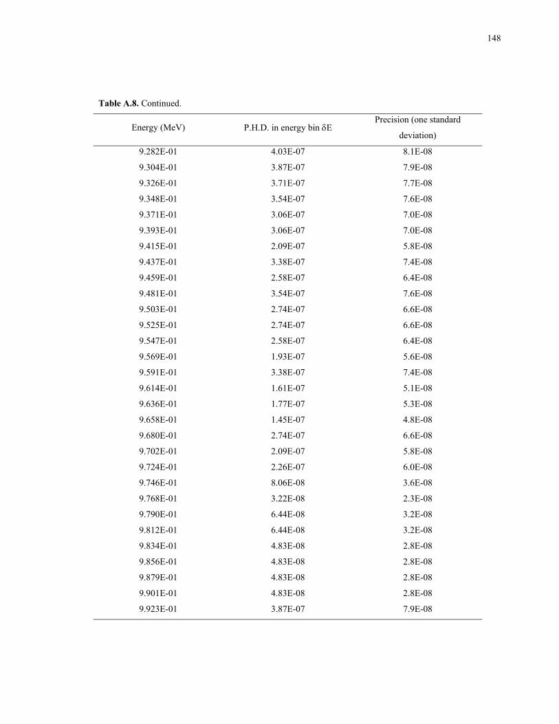
148
Table A.8. Continued.
Energy (MeV) P.H.D. in energy bin δE Precision (one standard
deviation)
9.282E-01 4.03E-07 8.1E-08
9.304E-01 3.87E-07 7.9E-08
9.326E-01 3.71E-07 7.7E-08
9.348E-01 3.54E-07 7.6E-08
9.371E-01 3.06E-07 7.0E-08
9.393E-01 3.06E-07 7.0E-08
9.415E-01 2.09E-07 5.8E-08
9.437E-01 3.38E-07 7.4E-08
9.459E-01 2.58E-07 6.4E-08
9.481E-01 3.54E-07 7.6E-08
9.503E-01 2.74E-07 6.6E-08
9.525E-01 2.74E-07 6.6E-08
9.547E-01 2.58E-07 6.4E-08
9.569E-01 1.93E-07 5.6E-08
9.591E-01 3.38E-07 7.4E-08
9.614E-01 1.61E-07 5.1E-08
9.636E-01 1.77E-07 5.3E-08
9.658E-01 1.45E-07 4.8E-08
9.680E-01 2.74E-07 6.6E-08
9.702E-01 2.09E-07 5.8E-08
9.724E-01 2.26E-07 6.0E-08
9.746E-01 8.06E-08 3.6E-08
9.768E-01 3.22E-08 2.3E-08
9.790E-01 6.44E-08 3.2E-08
9.812E-01 6.44E-08 3.2E-08
9.834E-01 4.83E-08 2.8E-08
9.856E-01 4.83E-08 2.8E-08
9.879E-01 4.83E-08 2.8E-08
9.901E-01 4.83E-08 2.8E-08
9.923E-01 3.87E-07 7.9E-08
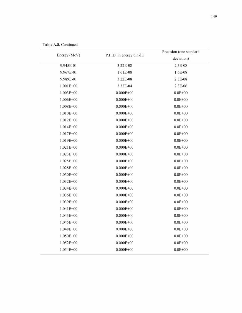
149
Table A.8. Continued.
Energy (MeV) P.H.D. in energy bin δE Precision (one standard
deviation)
9.945E-01 3.22E-08 2.3E-08
9.967E-01 1.61E-08 1.6E-08
9.989E-01 3.22E-08 2.3E-08
1.001E+00 3.32E-04 2.3E-06
1.003E+00 0.000E+00 0.0E+00
1.006E+00 0.000E+00 0.0E+00
1.008E+00 0.000E+00 0.0E+00
1.010E+00 0.000E+00 0.0E+00
1.012E+00 0.000E+00 0.0E+00
1.014E+00 0.000E+00 0.0E+00
1.017E+00 0.000E+00 0.0E+00
1.019E+00 0.000E+00 0.0E+00
1.021E+00 0.000E+00 0.0E+00
1.023E+00 0.000E+00 0.0E+00
1.025E+00 0.000E+00 0.0E+00
1.028E+00 0.000E+00 0.0E+00
1.030E+00 0.000E+00 0.0E+00
1.032E+00 0.000E+00 0.0E+00
1.034E+00 0.000E+00 0.0E+00
1.036E+00 0.000E+00 0.0E+00
1.039E+00 0.000E+00 0.0E+00
1.041E+00 0.000E+00 0.0E+00
1.043E+00 0.000E+00 0.0E+00
1.045E+00 0.000E+00 0.0E+00
1.048E+00 0.000E+00 0.0E+00
1.050E+00 0.000E+00 0.0E+00
1.052E+00 0.000E+00 0.0E+00
1.054E+00 0.000E+00 0.0E+00
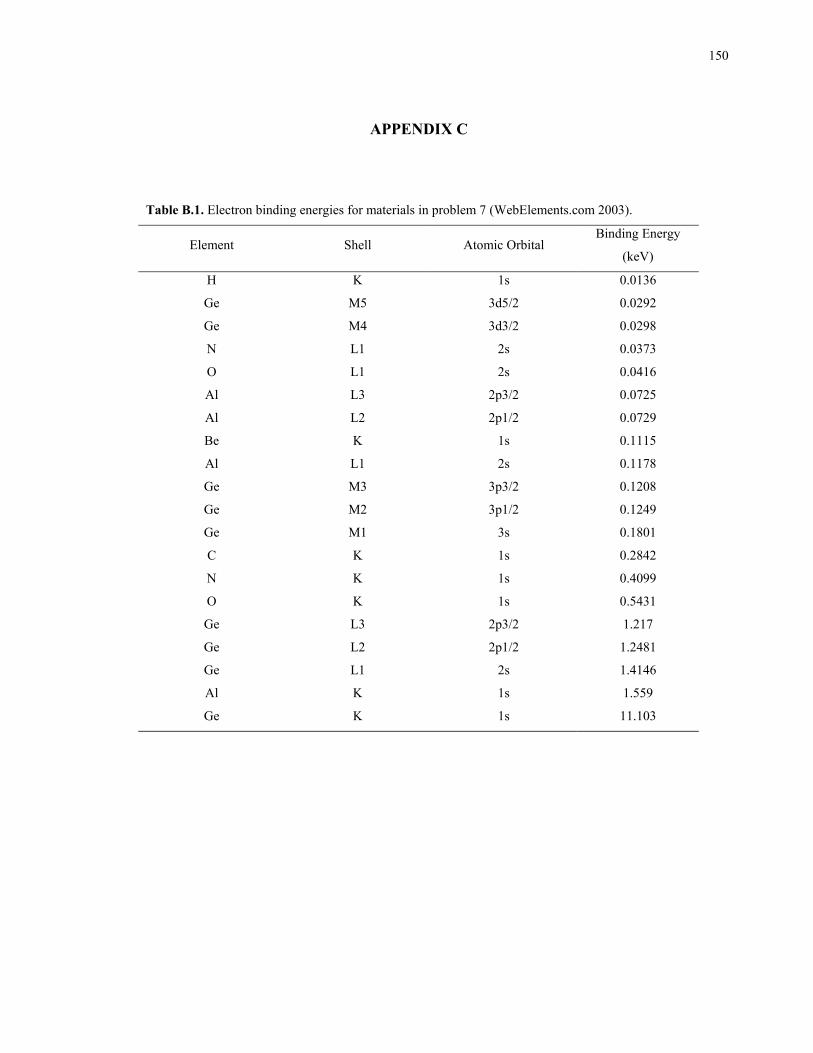
150
APPENDIX C
Table B.1. Electron binding energies for materials in problem 7 (WebElements.com 2003).
Element Shell Atomic Orbital Binding Energy
(keV)
H K 1s 0.0136
Ge M5 3d5/2 0.0292
Ge M4 3d3/2 0.0298
N L1 2s 0.0373
O L1 2s 0.0416
Al L3 2p3/2 0.0725
Al L2 2p1/2 0.0729
Be K 1s 0.1115
Al L1 2s 0.1178
Ge M3 3p3/2 0.1208
Ge M2 3p1/2 0.1249
Ge M1 3s 0.1801
C K 1s 0.2842
N K 1s 0.4099
O K 1s 0.5431
Ge L3 2p3/2 1.217
Ge L2 2p1/2 1.2481
Ge L1 2s 1.4146
Al K 1s 1.559
Ge K 1s 11.103
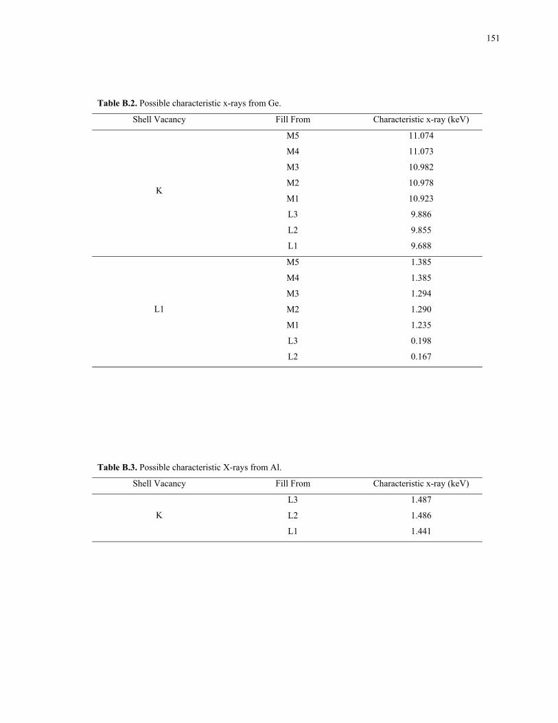
151
Table B.2. Possible characteristic x-rays from Ge.
Shell Vacancy Fill From Characteristic x-ray (keV)
M5 11.074
M4 11.073
M3 10.982
M2 10.978
M1 10.923
L3 9.886
L2 9.855
K
L1 9.688
M5 1.385
M4 1.385
M3 1.294
M2 1.290
M1 1.235
L3 0.198
L1
L2 0.167
Table B.3. Possible characteristic X-rays from Al.
Shell Vacancy Fill From Characteristic x-ray (keV)
L3 1.487
L2 1.486 K
L1 1.441
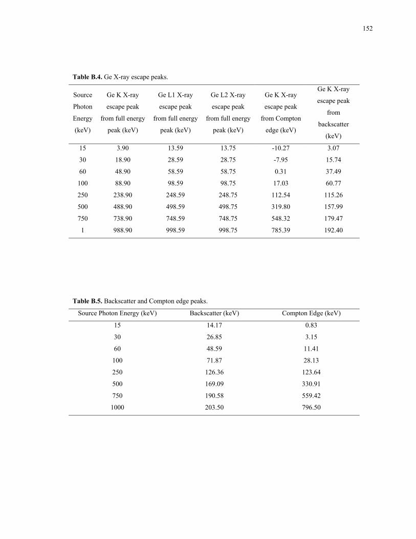
152
Table B.4. Ge X-ray escape peaks.
Source
Photon
Energy
(keV)
Ge K X-ray
escape peak
from full energy
peak (keV)
Ge L1 X-ray
escape peak
from full energy
peak (keV)
Ge L2 X-ray
escape peak
from full energy
peak (keV)
Ge K X-ray
escape peak
from Compton
edge (keV)
Ge K X-ray
escape peak
from
backscatter
(keV)
15 3.90 13.59 13.75 -10.27 3.07
30 18.90 28.59 28.75 -7.95 15.74
60 48.90 58.59 58.75 0.31 37.49
100 88.90 98.59 98.75 17.03 60.77
250 238.90 248.59 248.75 112.54 115.26
500 488.90 498.59 498.75 319.80 157.99
750 738.90 748.59 748.75 548.32 179.47
1 988.90 998.59 998.75 785.39 192.40
Table B.5. Backscatter and Compton edge peaks.
Source Photon Energy (keV) Backscatter (keV) Compton Edge (keV)
15 14.17 0.83
30 26.85 3.15
60 48.59 11.41
100 71.87 28.13
250 126.36 123.64
500 169.09 330.91
750 190.58 559.42
1000 203.50 796.50
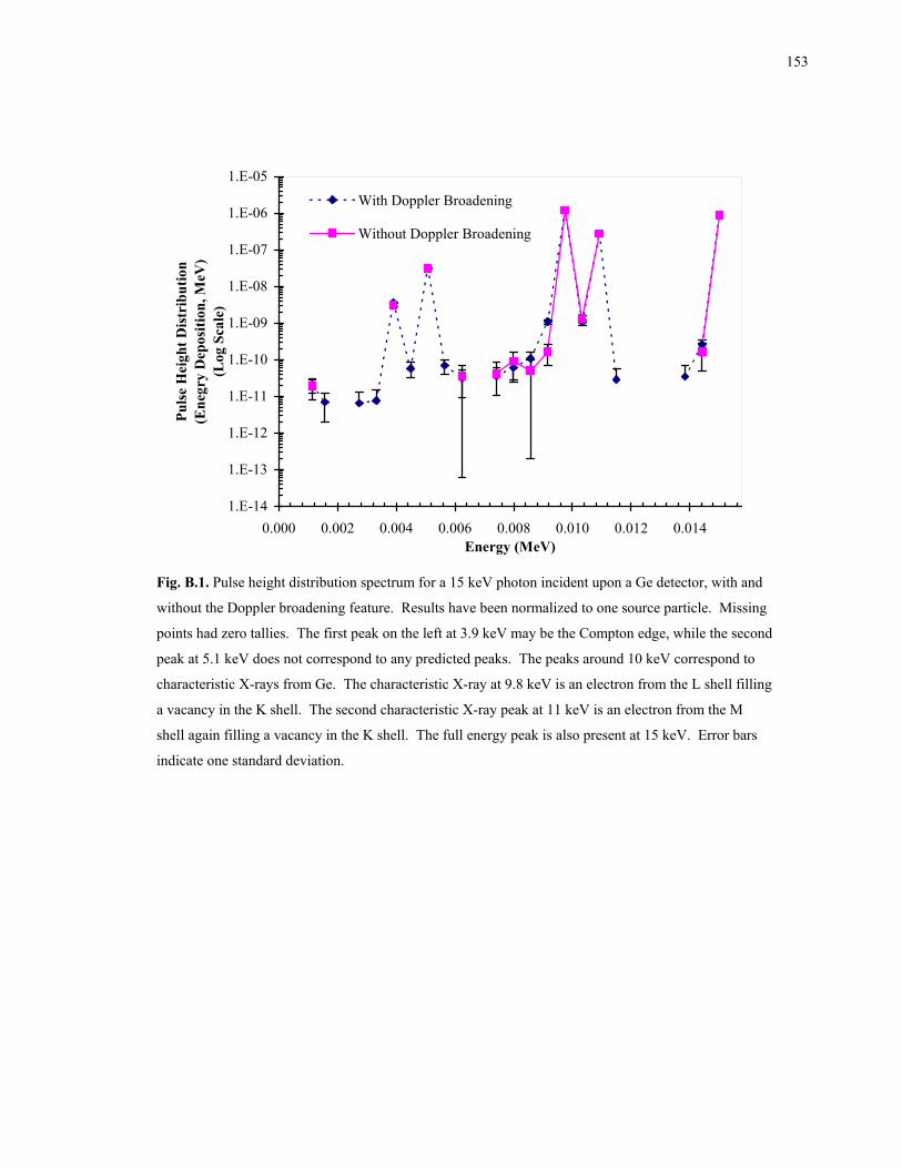
153
1.E-14
1.E-13
1.E-12
1.E-11
1.E-10
1.E-09
1.E-08
1.E-07
1.E-06
1.E-05
0.000 0.002 0.004 0.006 0.008 0.010 0.012 0.014Energy (MeV)
Puls
e H
eigh
t Dis
trib
utio
n(E
negr
y D
epos
ition
, MeV
)(L
og S
cale
)With Doppler Broadening
Without Doppler Broadening
Fig. B.1. Pulse height distribution spectrum for a 15 keV photon incident upon a Ge detector, with and
without the Doppler broadening feature. Results have been normalized to one source particle. Missing
points had zero tallies. The first peak on the left at 3.9 keV may be the Compton edge, while the second
peak at 5.1 keV does not correspond to any predicted peaks. The peaks around 10 keV correspond to
characteristic X-rays from Ge. The characteristic X-ray at 9.8 keV is an electron from the L shell filling
a vacancy in the K shell. The second characteristic X-ray peak at 11 keV is an electron from the M
shell again filling a vacancy in the K shell. The full energy peak is also present at 15 keV. Error bars
indicate one standard deviation.
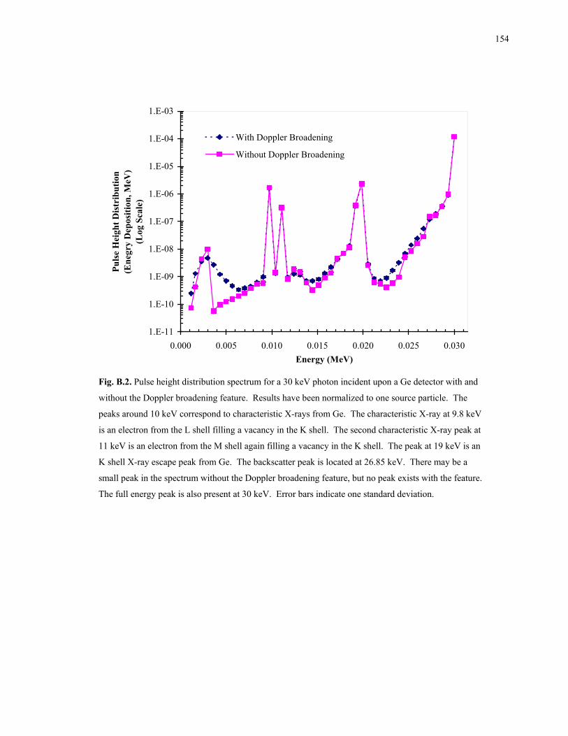
154
1.E-11
1.E-10
1.E-09
1.E-08
1.E-07
1.E-06
1.E-05
1.E-04
1.E-03
0.000 0.005 0.010 0.015 0.020 0.025 0.030Energy (MeV)
Puls
e H
eigh
t Dis
trib
utio
n(E
negr
y D
epos
ition
, MeV
)(L
og S
cale
)With Doppler Broadening
Without Doppler Broadening
Fig. B.2. Pulse height distribution spectrum for a 30 keV photon incident upon a Ge detector with and
without the Doppler broadening feature. Results have been normalized to one source particle. The
peaks around 10 keV correspond to characteristic X-rays from Ge. The characteristic X-ray at 9.8 keV
is an electron from the L shell filling a vacancy in the K shell. The second characteristic X-ray peak at
11 keV is an electron from the M shell again filling a vacancy in the K shell. The peak at 19 keV is an
K shell X-ray escape peak from Ge. The backscatter peak is located at 26.85 keV. There may be a
small peak in the spectrum without the Doppler broadening feature, but no peak exists with the feature.
The full energy peak is also present at 30 keV. Error bars indicate one standard deviation.
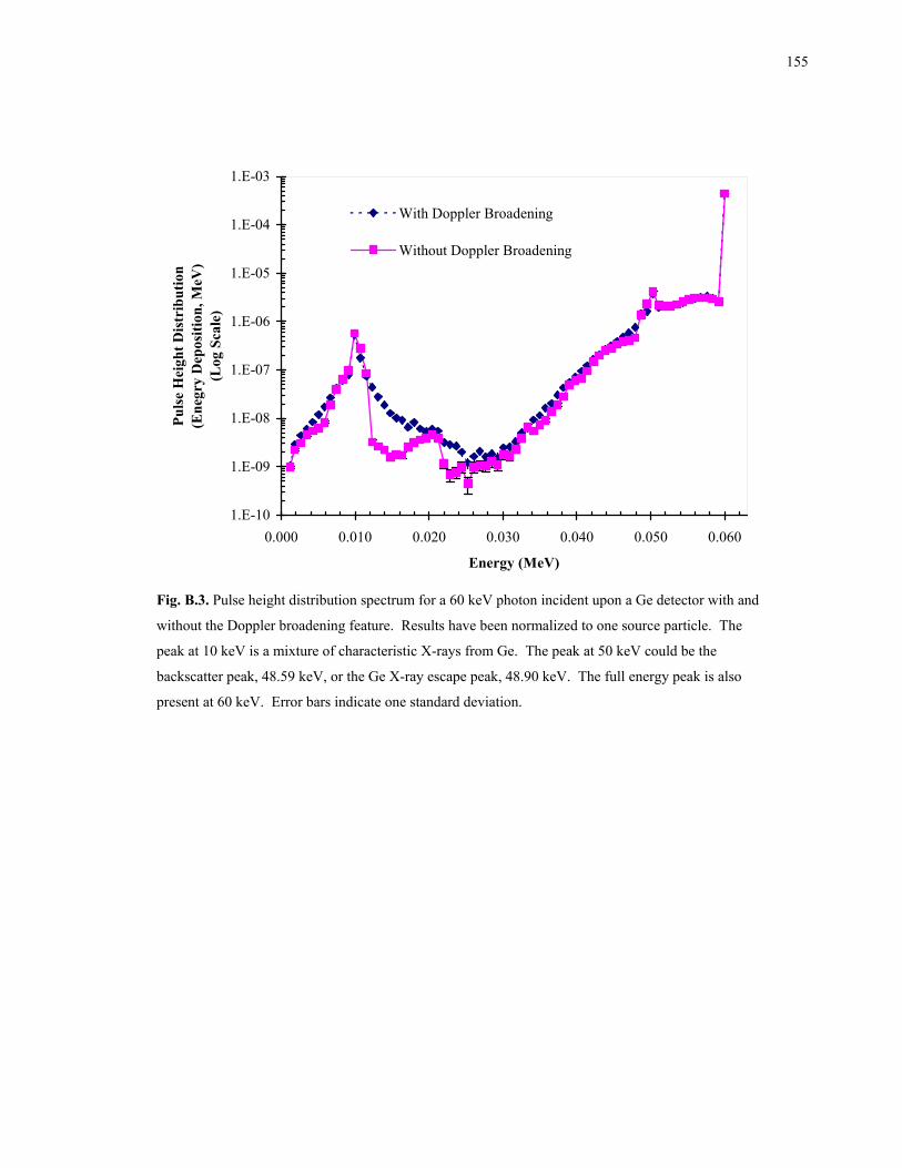
155
1.E-10
1.E-09
1.E-08
1.E-07
1.E-06
1.E-05
1.E-04
1.E-03
0.000 0.010 0.020 0.030 0.040 0.050 0.060
Energy (MeV)
Puls
e H
eigh
t Dis
trib
utio
n(E
negr
y D
epos
ition
, MeV
)(L
og S
cale
)With Doppler Broadening
Without Doppler Broadening
Fig. B.3. Pulse height distribution spectrum for a 60 keV photon incident upon a Ge detector with and
without the Doppler broadening feature. Results have been normalized to one source particle. The
peak at 10 keV is a mixture of characteristic X-rays from Ge. The peak at 50 keV could be the
backscatter peak, 48.59 keV, or the Ge X-ray escape peak, 48.90 keV. The full energy peak is also
present at 60 keV. Error bars indicate one standard deviation.
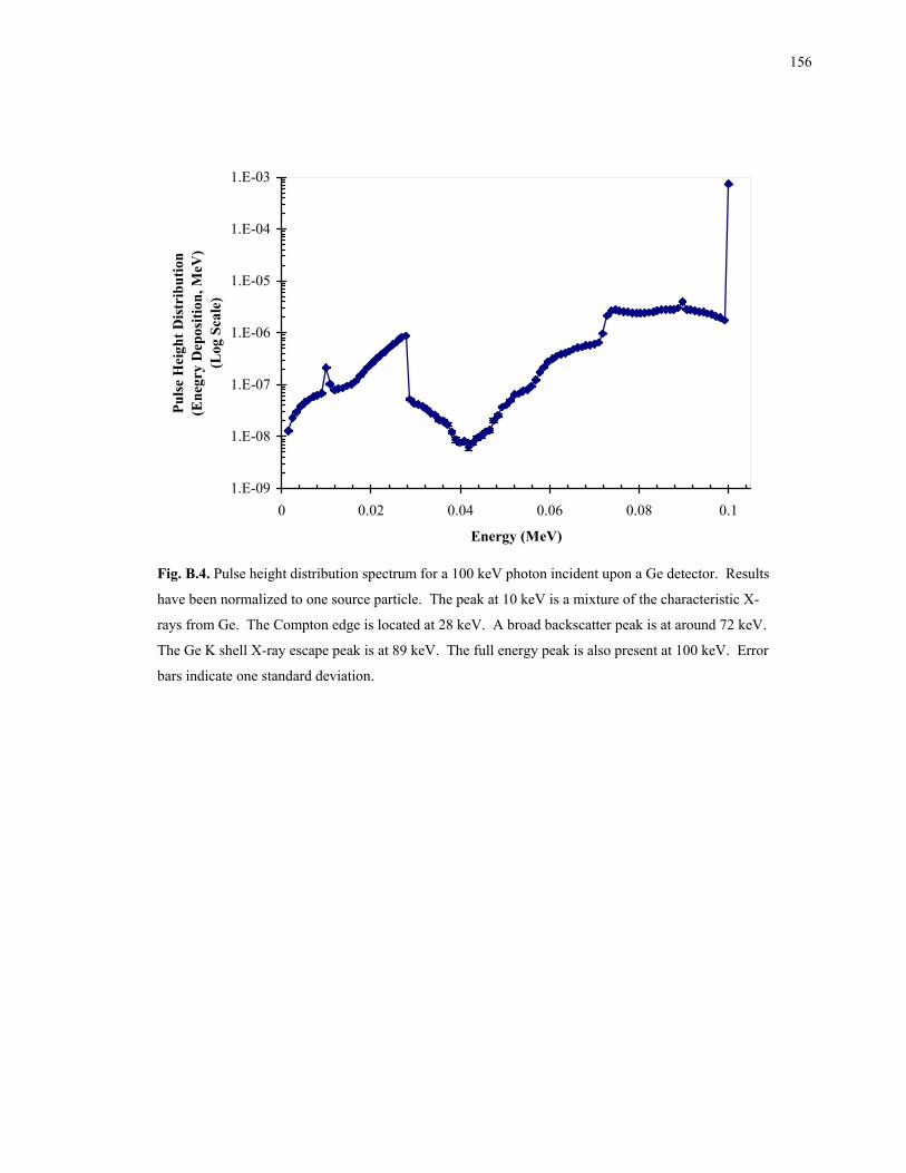
156
1.E-09
1.E-08
1.E-07
1.E-06
1.E-05
1.E-04
1.E-03
0 0.02 0.04 0.06 0.08 0.1
Energy (MeV)
Puls
e H
eigh
t Dis
trib
utio
n(E
negr
y D
epos
ition
, MeV
)(L
og S
cale
)
Fig. B.4. Pulse height distribution spectrum for a 100 keV photon incident upon a Ge detector. Results
have been normalized to one source particle. The peak at 10 keV is a mixture of the characteristic X-
rays from Ge. The Compton edge is located at 28 keV. A broad backscatter peak is at around 72 keV.
The Ge K shell X-ray escape peak is at 89 keV. The full energy peak is also present at 100 keV. Error
bars indicate one standard deviation.
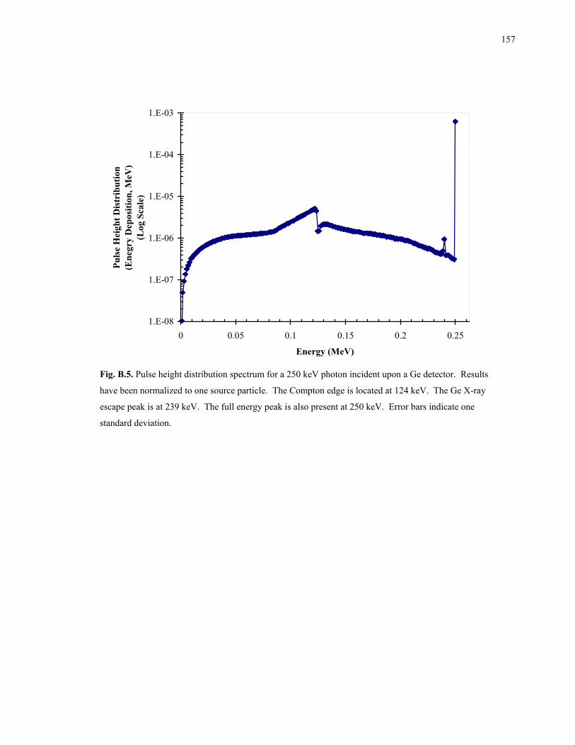
157
1.E-08
1.E-07
1.E-06
1.E-05
1.E-04
1.E-03
0 0.05 0.1 0.15 0.2 0.25
Energy (MeV)
Puls
e H
eigh
t Dis
trib
utio
n(E
negr
y D
epos
ition
, MeV
)(L
og S
cale
)
Fig. B.5. Pulse height distribution spectrum for a 250 keV photon incident upon a Ge detector. Results
have been normalized to one source particle. The Compton edge is located at 124 keV. The Ge X-ray
escape peak is at 239 keV. The full energy peak is also present at 250 keV. Error bars indicate one
standard deviation.
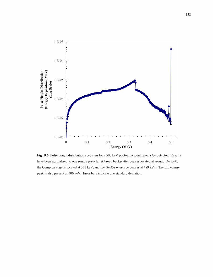
158
1.E-08
1.E-07
1.E-06
1.E-05
1.E-04
1.E-03
0 0.1 0.2 0.3 0.4 0.5Energy (MeV)
Puls
e H
eigh
t Dis
trib
utio
n(E
negr
y D
epos
ition
, MeV
)(L
og S
cale
)
Fig. B.6. Pulse height distribution spectrum for a 500 keV photon incident upon a Ge detector. Results
have been normalized to one source particle. A broad backscatter peak is located at around 169 keV,
the Compton edge is located at 331 keV, and the Ge X-ray escape peak is at 489 keV. The full energy
peak is also present at 500 keV. Error bars indicate one standard deviation.
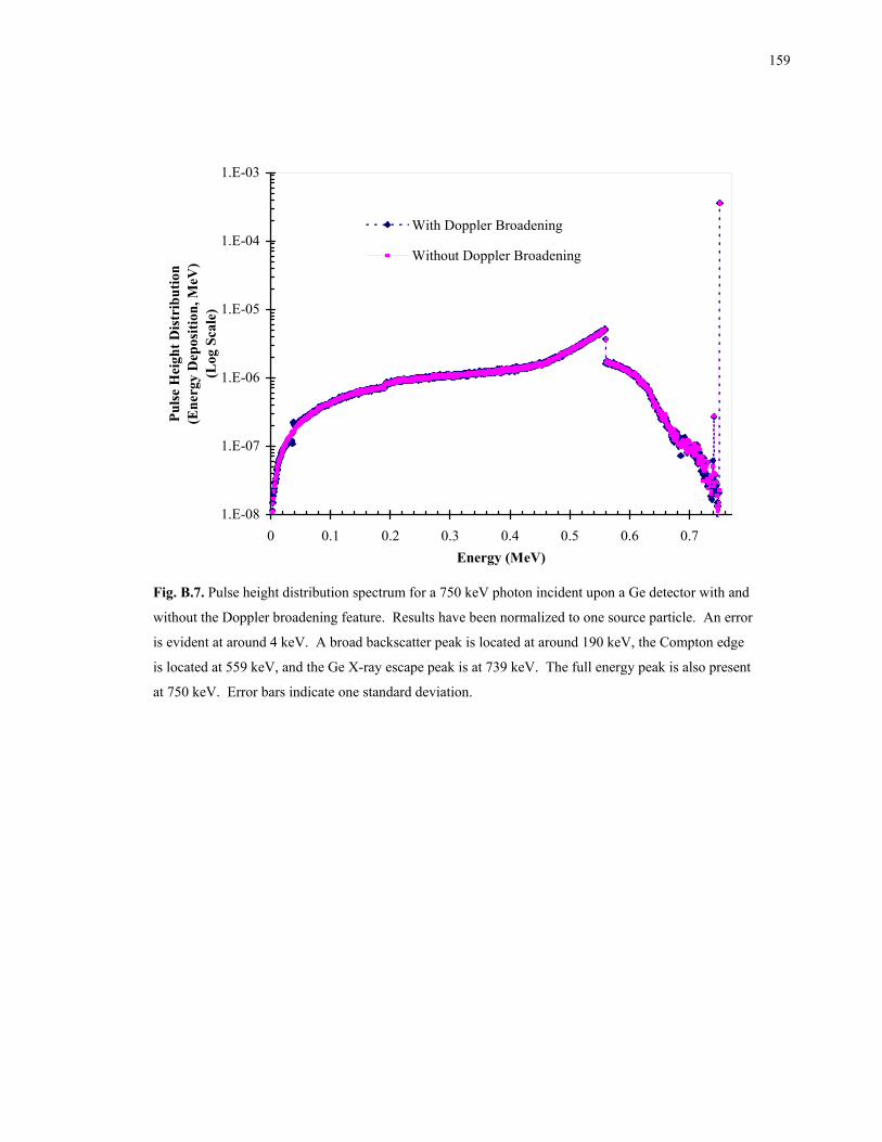
159
1.E-08
1.E-07
1.E-06
1.E-05
1.E-04
1.E-03
0 0.1 0.2 0.3 0.4 0.5 0.6 0.7Energy (MeV)
Puls
e H
eigh
t Dis
trib
utio
n(E
nerg
y D
epos
ition
, MeV
)(L
og S
cale
)With Doppler Broadening
Without Doppler Broadening
Fig. B.7. Pulse height distribution spectrum for a 750 keV photon incident upon a Ge detector with and
without the Doppler broadening feature. Results have been normalized to one source particle. An error
is evident at around 4 keV. A broad backscatter peak is located at around 190 keV, the Compton edge
is located at 559 keV, and the Ge X-ray escape peak is at 739 keV. The full energy peak is also present
at 750 keV. Error bars indicate one standard deviation.
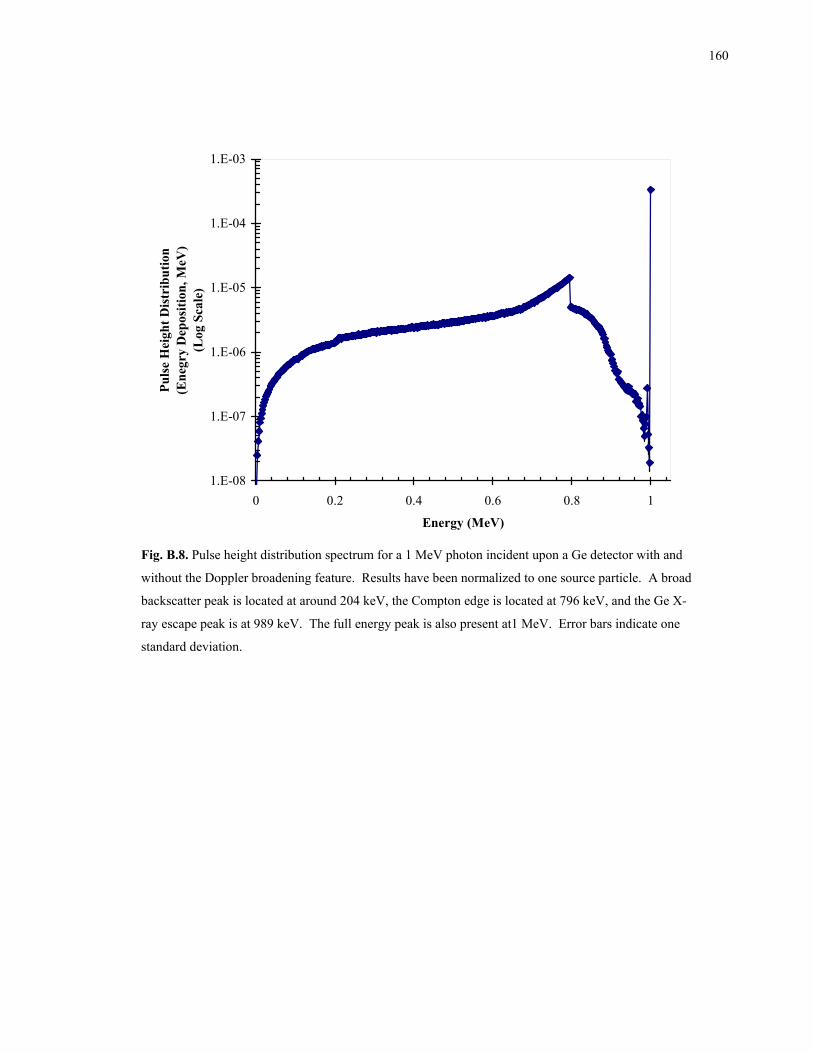
160
1.E-08
1.E-07
1.E-06
1.E-05
1.E-04
1.E-03
0 0.2 0.4 0.6 0.8 1
Energy (MeV)
Puls
e H
eigh
t Dis
trib
utio
n(E
negr
y D
epos
ition
, MeV
)(L
og S
cale
)
Fig. B.8. Pulse height distribution spectrum for a 1 MeV photon incident upon a Ge detector with and
without the Doppler broadening feature. Results have been normalized to one source particle. A broad
backscatter peak is located at around 204 keV, the Compton edge is located at 796 keV, and the Ge X-
ray escape peak is at 989 keV. The full energy peak is also present at1 MeV. Error bars indicate one
standard deviation.

161
VITA
R. Alex Redd received a Bachelor of Science degree in Chemistry from Texas A&M University
on December 17, 1994. After graduation he attends to continue his education at Texas A&M University.
His permanent address is 5247 Charing Way, Baton Rouge, LA 70817-2006.