radiation by moving charges - institut by moving charges may 27, 20081 1j.d.jackson, "classical...

Radiation by Moving Charges

May 27, 20081

1J.D.Jackson, ”Classical Electrodynamics”, 3rd Edition, Chapter 14Radiation by Moving Charges

Lienard - Wiechert Potentials

I The Lienard-Wiechert potential describes the electromagneticeffect of a moving charge.

I Built directly from Maxwell’s equations, this potential describes thecomplete, relativistically correct, time-varying electromagnetic fieldfor a point-charge in arbitrary motion.

I These classical equations harmonize with the 20th centurydevelopment of special relativity, but are not corrected forquantum-mechanical effects.

I Electromagnetic radiation in the form of waves are a natural resultof the solutions to these equations.

I These equations were developed in part by Emil Wiechert around1898 and continued into the early 1900s.


Lienard - Wiechert Potentials

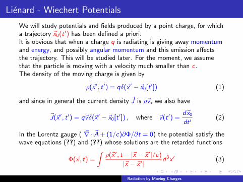
We will study potentials and fields produced by a point charge, for whicha trajectory ~x0(t ′) has been defined a priori.It is obvious that when a charge q is radiating is giving away momentumand energy, and possibly angular momentum and this emission affectsthe trajectory. This will be studied later. For the moment, we assumethat the particle is moving with a velocity much smaller than c .The density of the moving charge is given by

ρ(~x ′, t ′) = qδ(~x ′ − ~x0[t ′]) (1)

and since in general the current density ~J is ρ~v , we also have

~J(~x ′, t ′) = q~vδ(~x ′ − ~x0[t ′]) , where ~v(t ′) =d~x0

dt ′(2)

In the Lorentz gauge ( ~∇ · ~A + (1/c)∂Φ/∂t = 0) the potential satisfy thewave equations (??) and (??) whose solutions are the retarded functions

Φ(~x , t) =

∫ρ(~x ′, t − |~x − ~x ′|/c)

|~x − ~x ′|d3x ′ (3)


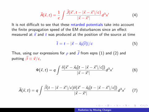
~A(~x , t) =1

c

∫ ~J(~x ′, t − |~x − ~x ′|/c)

|~x − ~x ′|d3x ′ (4)

It is not difficult to see that these retarded potentials take into accountthe finite propagation speed of the EM disturbances since an effectmeasured at ~x and t was produced at the position of the source at time

t = t − |~x − ~x0(t)|/c (5)

Thus, using our expressions for ρ and ~J from eqns (1) and (2) and

putting ~β ≡ ~v/c ,

Φ(~x , t) = q

∫δ(~x ′ − ~x0[t − |~x − ~x ′|/c])

|~x − ~x ′|d3x ′ (6)

~A(~x , t) = q

∫ ~β(t − |~x − ~x ′|/c)δ(~x ′ − ~x0[t − |~x − ~x ′|/c])

|~x − ~x ′|d3x ′ (7)


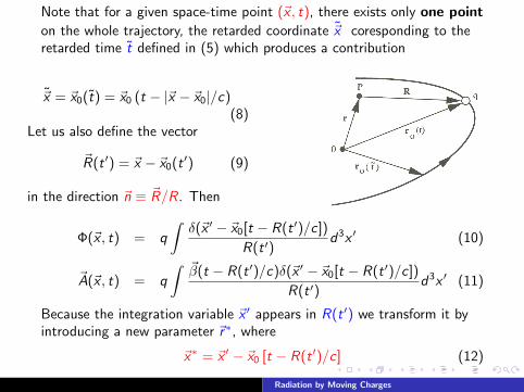
Note that for a given space-time point (~x , t), there exists only one point

on the whole trajectory, the retarded coordinate ~x coresponding to theretarded time t defined in (5) which produces a contribution

~x = ~x0(t) = ~x0 (t − |~x − ~x0|/c)(8)

Let us also define the vector

~R(t ′) = ~x − ~x0(t ′) (9)

in the direction ~n ≡ ~R/R. Then

Φ(~x , t) = q

∫δ(~x ′ − ~x0[t − R(t ′)/c])

R(t ′)d3x ′ (10)

~A(~x , t) = q

∫ ~β(t − R(t ′)/c)δ(~x ′ − ~x0[t − R(t ′)/c])

R(t ′)d3x ′ (11)

Because the integration variable ~x ′ appears in R(t ′) we transform it byintroducing a new parameter ~r∗, where

~x∗ = ~x ′ − ~x0 [t − R(t ′)/c] (12)


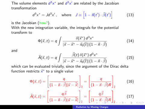
The volume elements d3x∗ and d3x ′ are related by the Jacobiantransfiormation

d3x∗ = Jd3x ′ , where J ≡[1− ~n(t ′) · ~β(t ′)

](13)

is the Jacobian (how?).With the new integration variable, the integrals for the potentialtransform to

Φ(~x , t) = q

∫δ(~x∗) d3x∗

|~x − ~x∗ − ~x0(t)|(1− ~n · ~β)(14)

and

~A(~x , t) = q

∫ ~β(t) δ(~x∗) d3x∗

|~x − ~x∗ − ~x0(t)|(1− ~n · ~β)(15)

which can be evaluated trivially, since the argument of the Dirac deltafunction restricts ~x∗ to a single value

Φ(~x , t) =

[q

(1− ~n · ~β)|~x − ~x |

]t

=

[q

(1− ~n · ~β)R

]t

(16)

~A(~x , t) =

[q~β

(1− ~n · ~β)|~x − ~x |

]t

=

[q~β

(1− ~n · ~β)R

]t

(17)


Lienard - Wiechert potentials

Φ(~x , t) =

[q

(1− ~n · ~β)|~x − ~x |

]t

=

[q

(1− ~n · ~β)R

]t

(18)

~A(~x , t) =

[q~β

(1− ~n · ~β)|~x − ~x |

]t

=

[q~β

(1− ~n · ~β)R

]t

(19)

These are the Lienard - Wiechert potentials.

It is worth noticing the presence of the term (1− ~n · ~β), which clearly

arises from the fact that the velocity of the EM waves is finite, so the

retardation effects must be taken into account in determining the fields.


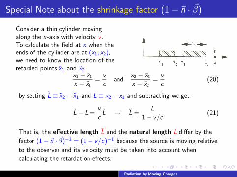
Special Note about the shrinkage factor (1− ~n · ~β)

Consider a thin cylinder movingalong the x-axis with velocity v .To calculate the field at x when theends of the cylinder are at (x1, x2),we need to know the location of theretarded points x1 and x2

x1 − x1

x − x1=

v

cand

x2 − x2

x − x2=

v

c(20)

by setting L ≡ x2 − x1 and L ≡ x2 − x1 and subtracting we get

L− L =v

cL → L =

L

1− v/c(21)

That is, the effective length L and the natural length L differ by the

factor (1− ~x · ~β)−1 = (1− v/c)−1 because the source is moving relative

to the observer and its velocity must be taken into account when

calculating the retardation effects.


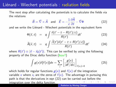
Lienard - Wiechert potentials : radiation fields

The next step after calculating the potentials is to calculate the fields viathe relations

~B = ~∇× ~A and ~E = −1

c

∂~A

∂t− ~∇Φ (22)

and we write the Lienard - Wiechert potentials in the equivalent form

Φ(~x , t) = q

∫δ(t ′ − t − R(t ′)/c)

R(t ′)dt ′ (23)

~A(~x , t) = q

∫ ~β(t ′)δ(t ′ − t + R(t ′)/c])

R(t ′)dt ′ (24)

where R(t ′) ≡ |~x − ~x0(t ′)|. This can be verified by using the followingproperty of the Dirac delta function (how?)∫

g(x)δ[f (x)]dx =∑

i

[g(x)

|df /dx |

]f (xi )=0

(25)

which holds for regular functions g(x) and f (x) of the integrationvariable x where xi are the zeros of f (x). The advantage in pursuing thispath is that the derivatives in eqn (22) can be carried out before theintegration over the delta function.


This procedure simplifies the evaluation of the fields considerably since,we do not need to keep track of the retarded time until the last step.We get for the electric field

~E (~x , t) = q

∫~∇[δ(t ′ − t + R(t ′)/c)

R(t ′)

]dt ′−q

c

∂

∂t

∫ ~β(t ′)δ(t ′ − t + R(t ′)/c)

R(t ′)(26)

Thus, differentiating the integrand in the first term, we get (HOW?)

~E (~x , t) = q

∫ [~n

R2δ

(t ′ − t +

R(t ′)

c

)−

~n

cRδ′(

t ′ − t +R(t ′)

c

)]dt ′

− q

c

∂

∂t

∫ ~β(t ′)δ(t ′ − t + R(t ′)/c)

R(t ′)(27)

But (HOW?)

δ′(

t ′ − t +R(t ′)

c

)= − ∂

∂tδ

(t ′ − t +

R(t ′)

c

)(28)

~E (~x , t) = q

∫~n

R2δ

(t ′ − t +

R(t ′)

c

)dt ′+

q

c

∂

∂t

∫(~n − ~β)

cR(t ′)δ

(t ′ − t +

R(t ′)

c

)dt ′

(29)


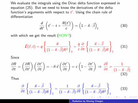
We evaluate the integrals using the Dirac delta function expressed inequation (25). But we need to know the derivatives of the deltafunction’s arguments with respect to t ′. Using the chain rule ofdifferentiation

d

dt ′

(t ′ − t +

R(t ′)

c

)=(

1− ~n · ~β)

t(30)

with which we get the result (HOW?):

~E (~r , t) = q

~n

(1− ~n · ~β)R2

t

+q

c

∂

∂t

~n − ~β

(1− ~n · ~β)R

t

(31)

Since

∂R

∂t=

(∂R

∂t ′

)(∂t ′

∂t

)= −~n·~v

(∂t ′

∂t

)= c

(1− ∂t ′

∂t

)⇒ ∂ t

∂t=

1

(1− ~n · ~β)(32)

Thus

∂

∂t

~n − ~β

(1− ~n · ~β)R

t

=1

(1− ~n · ~β)

∂

∂ t

~n − ~β

(1− ~n · ~β)R2

t

(33)


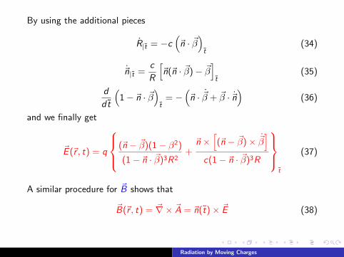
By using the additional pieces

R|t = −c(~n · ~β

)t

(34)

~n|t =c

R

[~n(~n · ~β)− ~β

]t

(35)

d

dt

(1− ~n · ~β

)t

= −(~n · ~β + ~β · ~n

)(36)

and we finally get

~E (~r , t) = q

(~n − ~β)(1− β2)

(1− ~n · ~β)3R2+~n ×

[(~n − ~β)× ~β

]c(1− ~n · ~β)3R

t

(37)

A similar procedure for ~B shows that

~B(~r , t) = ~∇× ~A = ~n(t)× ~E (38)


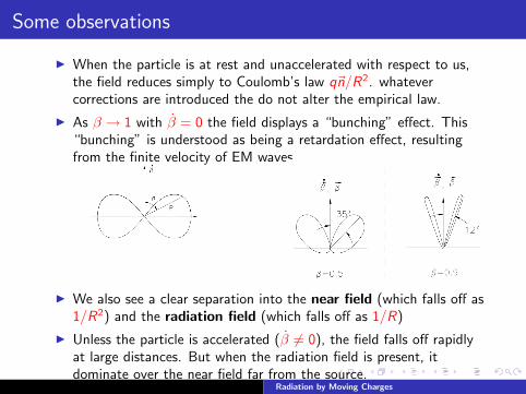
Some observations

I When the particle is at rest and unaccelerated with respect to us,the field reduces simply to Coulomb’s law q~n/R2. whatevercorrections are introduced the do not alter the empirical law.

I As β → 1 with β = 0 the field displays a “bunching” effect. This“bunching” is understood as being a retardation effect, resultingfrom the finite velocity of EM waves.

I We also see a clear separation into the near field (which falls off as1/R2) and the radiation field (which falls off as 1/R)

I Unless the particle is accelerated (β 6= 0), the field falls off rapidlyat large distances. But when the radiation field is present, itdominate over the near field far from the source.


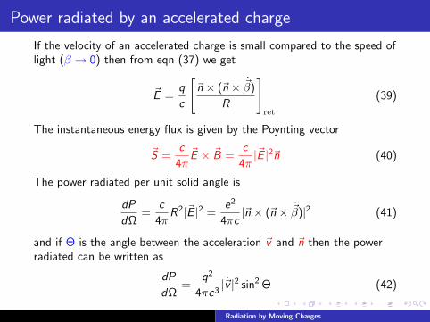
Power radiated by an accelerated charge

If the velocity of an accelerated charge is small compared to the speed oflight (β → 0) then from eqn (37) we get

~E =q

c

[~n × (~n × ~β)

R

]ret

(39)

The instantaneous energy flux is given by the Poynting vector

~S =c

4π~E × ~B =

c

4π|~E |2~n (40)

The power radiated per unit solid angle is

dP

dΩ=

c

4πR2|~E |2 =

e2

4πc|~n × (~n × ~β)|2 (41)

and if Θ is the angle between the acceleration ~v and ~n then the powerradiated can be written as

dP

dΩ=

q2

4πc3|~v |2 sin2 Θ (42)


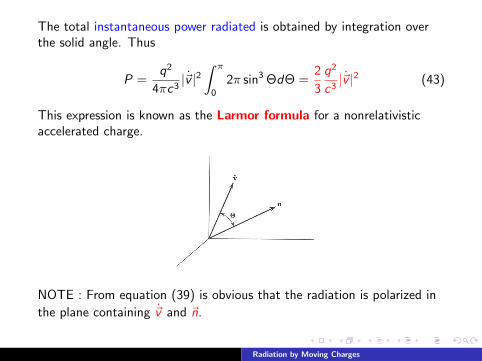
The total instantaneous power radiated is obtained by integration overthe solid angle. Thus

P =q2

4πc3|~v |2

∫ π

0

2π sin3 ΘdΘ =2

3

q2

c3|~v |2 (43)

This expression is known as the Larmor formula for a nonrelativisticaccelerated charge.

NOTE : From equation (39) is obvious that the radiation is polarized in

the plane containing ~v and ~n.


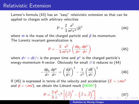
Relativistic Extension

Larmor’s formula (43) has an “easy” relativistic extension so that can beapplied to charges with arbitrary velocities

P =2

3

e2

m2c3|~p|2 (44)

where m is the mass of the charged particle and ~p its momentum.The Lorentz invariant generalization is

P = −2

3

e2

m2c3

(dpµdτ

dpµ

dτ

)(45)

where dτ = dt/γ is the proper time and pµ is the charged particle’senergy-momentum 4-vector. Obviously for small β it reduces to (44)

−dpµdτ

dpµ

dτ=

(d~p

dτ

)2

− 1

c2

(dE

dτ

)2

(46)

If (45) is expressed in terms of the velocity and acceleration (E = γmc2

and ~p = γm~v), we obtain the Lienard result (HOW?)

P =2

3

e2

cγ6

[(~β)2

−(~β × ~β

)2]

(47)


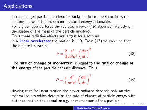
Applications

In the charged-particle accelerators radiation losses are sometimes thelimiting factor in the maximum practical energy attainable.For a given applied force the radiated paower (45) depends inversely onthe square of the mass of the particle involved.Thus these radiative effects are largest for electrons.In a linear accelerator the motion is 1-D. From (46) we can find thatthe radiated power is

P =2

3

e2

m2c3

(dp

dt

)2

(48)

The rate of change of momentum is equal to the rate of change ofthe energy of the particle per unit distance. Thus

P =2

3

e2

m2c3

(dE

dx

)2

(49)

slowing that for linear motion the power radiated depends only on theexternal forces which determine the rate of change of particle energy withdistance, not on the actual energy or momentum of the particle.


The ratio of power radiated to power supplied by external sources is

P

dE/dt=

2

3

e2

m2c3

1

v

dE

dx→ 2

3

(e2/mc2)

mc2

dE

dx(50)

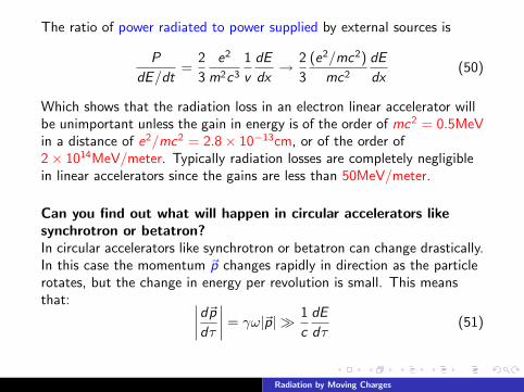
Which shows that the radiation loss in an electron linear accelerator willbe unimportant unless the gain in energy is of the order of mc2 = 0.5MeVin a distance of e2/mc2 = 2.8× 10−13cm, or of the order of2× 1014MeV/meter. Typically radiation losses are completely negligiblein linear accelerators since the gains are less than 50MeV/meter.

Can you find out what will happen in circular accelerators likesynchrotron or betatron?In circular accelerators like synchrotron or betatron can change drastically.In this case the momentum ~p changes rapidly in direction as the particlerotates, but the change in energy per revolution is small. This meansthat: ∣∣∣∣d~pdτ

∣∣∣∣ = γω|~p| 1

c

dE

dτ(51)


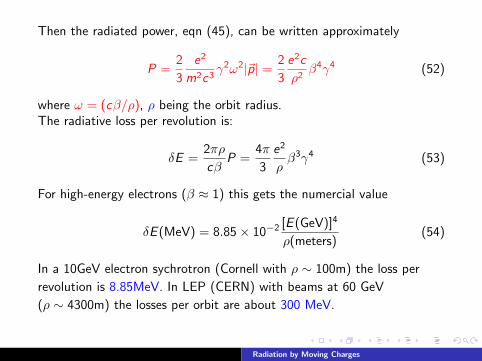
Then the radiated power, eqn (45), can be written approximately

P =2

3

e2

m2c3γ2ω2|~p| =

2

3

e2c

ρ2β4γ4 (52)

where ω = (cβ/ρ), ρ being the orbit radius.The radiative loss per revolution is:

δE =2πρ

cβP =

4π

3

e2

ρβ3γ4 (53)

For high-energy electrons (β ≈ 1) this gets the numercial value

δE (MeV) = 8.85× 10−2 [E (GeV)]4

ρ(meters)(54)

In a 10GeV electron sychrotron (Cornell with ρ ∼ 100m) the loss per

revolution is 8.85MeV. In LEP (CERN) with beams at 60 GeV

(ρ ∼ 4300m) the losses per orbit are about 300 MeV.


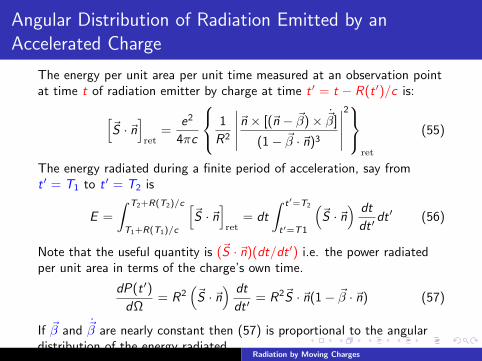
Angular Distribution of Radiation Emitted by anAccelerated Charge

The energy per unit area per unit time measured at an observation pointat time t of radiation emitter by charge at time t ′ = t − R(t ′)/c is:[

~S · ~n]

ret=

e2

4πc

1

R2

∣∣∣∣∣~n × [(~n − ~β)× ~β]

(1− ~β · ~n)3

∣∣∣∣∣2

ret

(55)

The energy radiated during a finite period of acceleration, say fromt ′ = T1 to t ′ = T2 is

E =

∫ T2+R(T2)/c

T1+R(T1)/c

[~S · ~n

]ret

= dt

∫ t′=T2

t′=T1

(~S · ~n

) dt

dt ′dt ′ (56)

Note that the useful quantity is (~S · ~n)(dt/dt ′) i.e. the power radiatedper unit area in terms of the charge’s own time.

dP(t ′)

dΩ= R2

(~S · ~n

) dt

dt ′= R2~S · ~n(1− ~β · ~n) (57)

If ~β and ~β are nearly constant then (57) is proportional to the angulardistribution of the energy radiated.


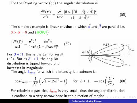
For the Poynting vector (55) the angular distribution is

dP(t ′)

dΩ=

e2

4πc

|~n × (~n − ~β)× ~β|2

(1− ~n · ~β)5(58)

The simplest example is linear motion in which ~β and ~β are parallel i.e.~β × ~β = 0 and (HOW?)

dP(t ′)

dΩ=

e2v2

4πc3

sin2 θ

(1− β cos θ)5(59)

For β 1, this is the Larmor result(42). But as β → 1, the angulardistribution is tipped forward andincreases in magnitude.

The angle θmax for which the intensity is maximum is:

cos θmax =1

3β

(√1 + 15β2 − 1

)for β ≈ 1 → cos

(1

2γ

)(60)

For relativistic particles, θmax is very small, thus the angular distribution

is confined to a very narrow cone in the direction of motion.


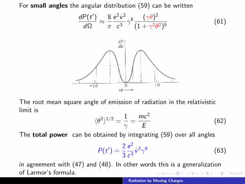
For small angles the angular distribution (59) can be written

dP(t ′)

dΩ≈ 8

π

e2v2

c3γ8 (γθ)2

(1 + γ2θ2)5(61)

The root mean square angle of emission of radiation in the relativisticlimit is

〈θ2〉1/2 =1

γ=

mc2

E(62)

The total power can be obtained by integrating (59) over all angles

P(t ′) =2

3

e2

c3v2γ6 (63)

in agreement with (47) and (48). In other words this is a generalizationof Larmor’s formula.


It is instructive to express this is terms of the force acting on the particle.This force is ~F = d~p/dt where ~p = mγ~v is the particle’s relativisticmomentum. For linear motion in the x-direction we have px = mvγ and

dpx

dt= mvγ + mvβ2γ3 = mvγ3

and Larmor’s formula can be written as

P =2

3

e2

c3

|~F |2

m2(64)

This is the total charge radiated by a charge in instantaneous linear

motion.


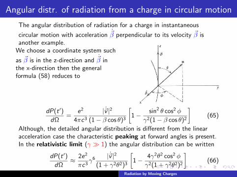
Angular distr. of radiation from a charge in circular motion

The angular distribution of radiation for a charge in instantaneous

circular motion with acceleration ~β perpendicular to its velocity ~β isanother example.

We choose a coordinate system such

as ~β is in the z-direction and ~β inthe x-direction then the generalformula (58) reduces to

dP(t ′)

dΩ=

e2

4πc3

|~v |2

(1− β cos θ)3

[1− sin2 θ cos2 φ

γ2(1− β cos θ)2

](65)

Although, the detailed angular distribution is different from the linearacceleration case the characteristic peaking at forward angles is present.In the relativistic limit (γ 1) the angular distribution can be written

dP(t ′)

dΩ≈ 2e2

πc3γ6 |~v |2

(1 + γ2θ2)3

[1− 4γ2θ2 cos2 φ

γ2(1 + γ2θ2)2

](66)


The root mean square angle of emission in this approximation is similarto (62) just as in the 1-dimensional motion. (SHOW IT?)The total power radiated can be found by integrating (65) over allangles or from (47)

P(t ′) =2

3

e2|~v |2

c3γ4 (67)

Since, for circular motion, the magnitude of the rate of momentum isequal to the force i.e. γm~v we can rewrite (67) as

Pcircular(t ′) =2

3

e2

m2c3γ2

(d~p

dt

)2

(68)

If we compare with the corresponding result (48) for rectilinear

motion, we find that the radiation emitted with a transverse

acceleration is a factor γ2 larger than with a parallel acceleration.


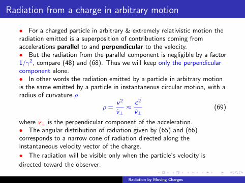
Radiation from a charge in arbitrary motion

• For a charged particle in arbitrary & extremely relativistic motion theradiation emitted is a superposition of contributions coming fromaccelerations parallel to and perpendicular to the velocity.• But the radiation from the parallel component is negligible by a factor1/γ2, compare (48) and (68). Thus we will keep only the perpendicularcomponent alone.• In other words the radiation emitted by a particle in arbitrary motionis the same emitted by a particle in instantaneous circular motion, with aradius of curvature ρ

ρ =v2

v⊥≈ c2

v⊥(69)

where v⊥ is the perpendicular component of the acceleration.• The angular distribution of radiation given by (65) and (66)corresponds to a narrow cone of radiation directed along theinstantaneous velocity vector of the charge.

• The radiation will be visible only when the particle’s velocity is

directed toward the observer.


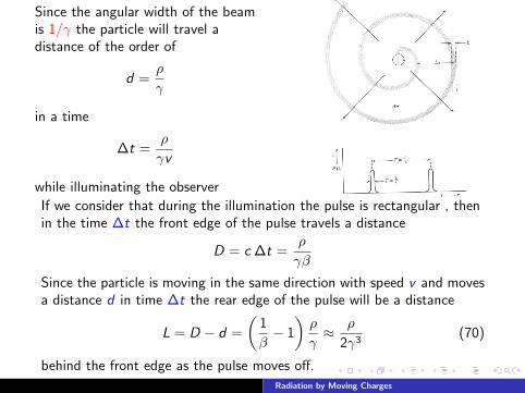
Since the angular width of the beamis 1/γ the particle will travel adistance of the order of

d =ρ

γ

in a time

∆t =ρ

γv

while illuminating the observer

If we consider that during the illumination the pulse is rectangular , thenin the time ∆t the front edge of the pulse travels a distance

D = c ∆t =ρ

γβ

Since the particle is moving in the same direction with speed v and movesa distance d in time ∆t the rear edge of the pulse will be a distance

L = D − d =

(1

β− 1

)ρ

γ≈ ρ

2γ3(70)

behind the front edge as the pulse moves off.


The Fourier decomposition of a finite wave train, we can find that thespectrum of the radiation will contain appreciable frequency componentsup to a critical frequency,

ωc ∼c

L∼(

c

ρ

)γ3 (71)

• For circular motion the term c/ρ is the angular frequency of rotationω0 and even for arbitrary motion plays the role of the fundamentalfrequency.• This shows that a relativistic particle emits a broad spectrum offrequencies up to γ3 times the fundamental frequency.

• EXAMPLE : In a 200MeV sychrotron, γmax ≈ 400, while

ω0 ≈ 3× 108s−1. The frequency spectrum of emitted radiation extends

up to ω ≈ 2× 1016s−1.


Distribution in Frequency and Angle of Energy Radiated ...

• The previous qualitative arguments show that for relativistic motionthe radiated energy is spread over a wide range of frequencies.• The estimation can be made precise and quantidative by use ofParseval’s theorem of Fourier analysis.The general form of the power radiated per unit solid angle is

dP(t)

dΩ= |~A(t)|2 (72)

where~A(t) =

( c

4π

)2 [R ~E

]ret

(73)

and ~E is the electric field defined in (37).• Notice that here we will use the observer’s time instead of theretarded time since we study the observed spectrum.The total energy radiated per unit solid angle is the time integral of (72):

dW

dΩ=

∫ ∞−∞|~A(t)|2dt (74)

This can be expressed via the Fourier transform’s as an integral over the

frequency.Radiation by Moving Charges

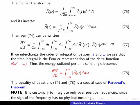
The Fourier transform is:

~A(ω) =1√2π

∫ ∞−∞

~A(t)e iωtdt (75)

and its inverse:~A(t) =

1√2π

∫ ∞−∞

~A(ω)e−iωtdω (76)

Then eqn (74) can be written

dW

dΩ=

1

2π

∫ ∞−∞

dt

∫ ∞−∞

dω

∫ ∞−∞

dω′~A∗(ω′) · ~A(ω)e i(ω′−ω)t (77)

If we interchange the order of integration between t and ω we see thatthe time integral is the Fourier represendation of the delta functionδ(ω′ − ω). Thus the energy radiated per unit solid angle becomes

dW

dΩ=

∫ ∞−∞|~A(ω)|2dω (78)

The equality of equations (74) and (78) is a special case of Parseval’stheorem.

NOTE: It is customary to integrate only over positive frequencies, since

the sign of the frequency has no physical meaning.


The energy radiated per unit solid angle per unit frequency interval is

dW

dΩ=

∫ ∞0

d2I (ω,~n)

dωdΩdω (79)

whered2I

dωdΩ= |~A(ω)|2 + |~A(−ω)|2 (80)

If ~A(t) is real, form (75) - (76) it is evident that ~A(−ω) = ~A∗(ω). Then

d2I

dωdΩ= 2|~A(ω)|2 (81)

which relates the power radiated as a funtion of time to the frequencyspectrum of the energy radiated.NOTE : We rewrite eqn (37) for future use

~E (~r , t) = e

~n − ~β

γ2(1− ~n · ~β)3R2+~n ×

[(~n − ~β)× ~β

]c(1− ~n · ~β)3R

ret

(82)


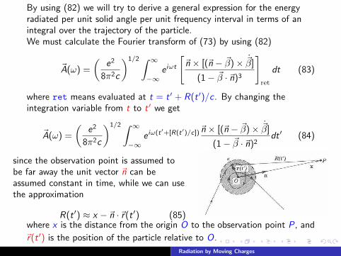
By using (82) we will try to derive a general expression for the energyradiated per unit solid angle per unit frequency interval in terms of anintegral over the trajectory of the particle.We must calculate the Fourier transform of (73) by using (82)

~A(ω) =

(e2

8π2c

)1/2 ∫ ∞−∞

e iωt

[~n × [(~n − ~β)× ~β]

(1− ~β · ~n)3

]ret

dt (83)

where ret means evaluated at t = t ′ + R(t ′)/c . By changing theintegration variable from t to t ′ we get

~A(ω) =

(e2

8π2c

)1/2 ∫ ∞−∞

e iω(t′+[R(t′)/c])~n × [(~n − ~β)× ~β]

(1− ~β · ~n)2dt ′ (84)

since the observation point is assumed tobe far away the unit vector ~n can beassumed constant in time, while we can usethe approximation

R(t ′) ≈ x − ~n ·~r(t ′) (85)where x is the distance from the origin O to the observation point P, and

~r(t ′) is the position of the particle relative to O.


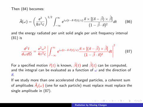
Then (84) becomes:

~A(ω) =

(e2

8π2c

)1/2 ∫ ∞−∞

e iω(t−~n·~r(t)/c)~n × [(~n − ~β)× ~β]

(1− ~β · ~n)2dt (86)

and the energy radiated per unit solid angle per unit frequency interval(81) is

d2I

dωdΩ=

e2ω2

4π2c

∣∣∣∣∣∫ ∞−∞

e iω(t−~n·~r(t)/c)~n × [(~n − ~β)× ~β]

(1− ~β · ~n)2dt

∣∣∣∣∣2

(87)

For a specified motion ~r(t) is known, ~β(t) and ~β(t) can be computed,and the integral can be evaluated as a function of ω and the direction of~n.

If we study more than one accelerated charged particles, a coherent sum

of amplitudes ~Aj(ω) (one for each particle) must replace must replace the

single amplitude in (87).


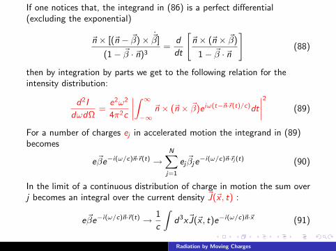
If one notices that, the integrand in (86) is a perfect differential(excluding the exponential)

~n × [(~n − ~β)× ~β]

(1− ~β · ~n)3=

d

dt

[~n × (~n × ~β)

1− ~β · ~n

](88)

then by integration by parts we get to the following relation for theintensity distribution:

d2I

dωdΩ=

e2ω2

4π2c

∣∣∣∣∫ ∞−∞

~n × (~n × ~β)e iω(t−~n·~r(t)/c)dt

∣∣∣∣2 (89)

For a number of charges ej in accelerated motion the integrand in (89)becomes

e~βe−i(ω/c)~n·~r(t) →N∑

j=1

ej~βje−i(ω/c)~n·~rj (t) (90)

In the limit of a continuous distribution of charge in motion the sum overj becomes an integral over the current density ~J(~x , t) :

e~βe−i(ω/c)~n·~r(t) → 1

c

∫d3x~J(~x , t)e−i(ω/c)~n·~x (91)


Then the intensity distribution becomes:

d2I

dωdΩ=

ω2

4π2c3

∣∣∣∣∫ dt

∫d3x e iω(t−~n·~x/c)~n × [~n × ~J(~x , t)]

∣∣∣∣2 (92)

a result that can be obtained from the direct solution of the

inhomogeneous wave equation for the vector potential.


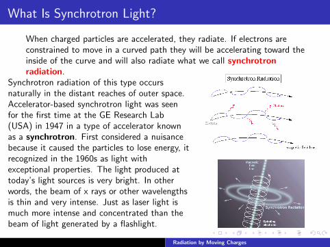
What Is Synchrotron Light?

When charged particles are accelerated, they radiate. If electrons areconstrained to move in a curved path they will be accelerating toward theinside of the curve and will also radiate what we call synchrotronradiation.

Synchrotron radiation of this type occursnaturally in the distant reaches of outer space.Accelerator-based synchrotron light was seenfor the first time at the GE Research Lab(USA) in 1947 in a type of accelerator knownas a synchrotron. First considered a nuisancebecause it caused the particles to lose energy, itrecognized in the 1960s as light withexceptional properties. The light produced attoday’s light sources is very bright. In otherwords, the beam of x rays or other wavelengthsis thin and very intense. Just as laser light ismuch more intense and concentrated than thebeam of light generated by a flashlight.


Synchrotrons

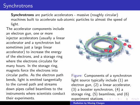
Synchrotrons are particle accelerators - massive (roughly circular)machines built to accelerate sub-atomic particles to almost the speed oflight.

The accelerator components includean electron gun, one or moreinjector accelerators (usually a linearaccelerator and a synchrotron butsometimes just a large linearaccelerator) to increase the energyof the electrons, and a storage ringwhere the electrons circulate formany hours. In the storage ring,magnets force the electrons intocircular paths. As the electron pathbends, light is emitted tangentiallyto the curved path and streamsdown pipes called beamlines to theinstruments where scientists conducttheir experiments.

Figure: Components of a synchrotronlight source typically include (1) anelectron gun, (2) a linear accelerator,(3) a booster synchrotron, (4) astorage ring, (5) beamlines, and (6)experiment stations.


Synchrotrons

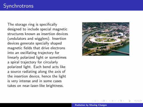
The storage ring is specificallydesigned to include special magneticstructures known as insertion devices(undulators and wigglers). Insertiondevices generate specially shapedmagnetic fields that drive electronsinto an oscillating trajectory forlinearly polarized light or sometimesa spiral trajectory for circularlypolarized light. Each bend acts likea source radiating along the axis ofthe insertion device, hence the lightis very intense and in some casestakes on near-laser-like brightness.


Synchrotron Radiation

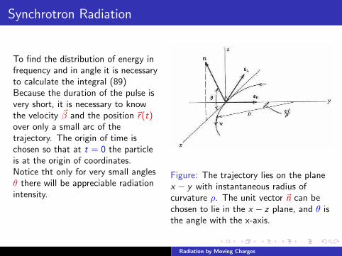
To find the distribution of energy infrequency and in angle it is necessaryto calculate the integral (89)Because the duration of the pulse isvery short, it is necessary to knowthe velocity ~β and the position ~r(t)over only a small arc of thetrajectory. The origin of time ischosen so that at t = 0 the particleis at the origin of coordinates.Notice tht only for very small anglesθ there will be appreciable radiationintensity.

Figure: The trajectory lies on the planex − y with instantaneous radius ofcurvature ρ. The unit vector ~n can bechosen to lie in the x − z plane, and θ isthe angle with the x-axis.


The vector part of the integrand in eqn (89) can be written

~n × (~n × ~β) = β[−~ε‖ sin(vt/ρ) + ~ε⊥ cos(vt/ρ) sin θ

](93)

~ε‖ = ~ε2 is a unit vector in the y -direction, corresponding to thepolarization in the plane of the orbit~ε⊥ = ~n × ~ε2 is the orthogonal polarization vector corresponding approx.to polarization perpendicular to the orbit plane (for small θ).The argument of the exponential is

ω

(t −

~n ·~r(t)

c

)= ω

[t − ρ

csin

(vt

ρ

)cos θ

](94)

Since we are dealing with small angle θ and very short time intervals wecan make an expansion to both trigonometric functions to obtain

ω

(t −

~n ·~r(t)

c

)≈ ω

2

[(1

γ2+ θ2

)t +

c2

3ρ2t3

](95)

where β was set to unity wherever possible.

CHECK THE ABOVE RELATIONS


Thus the radiated energy distribution (89) can be written

d2I

dωdΩ=

e2ω2

4π2c

∣∣−~ε‖A‖(ω) + ~ε⊥A⊥(ω)∣∣2 (96)

where the two amplitudes are (How?)

A‖(ω) ≈ c

ρ

∫ ∞−∞

t exp

iω

2

[(1

γ2+ θ2

)t +

c2t3

3ρ2

]dt (97)

A⊥(ω) ≈ θ

∫ ∞−∞

exp

iω

2

[(1

γ2+ θ2

)t +

c2t3

3ρ2

]dt (98)

by changing the integration variable

x =ct

ρ(1/γ2 + θ2)1/2

and introducing the parameter ξ

ξ =ωρ

3c

(1

γ2+ θ2

)3/2

(99)

allows us to transform the integrals into the form


A‖(ω) ≈ ρ

c

(1

γ2+ θ2

)∫ ∞−∞

x exp[i3

2ξ

(x +

1

3x3

)]dx (100)

A⊥(ω) ≈ ρ

cθ

(1

γ2+ θ2

)1/2 ∫ ∞−∞

exp[i3

2ξ

(x +

1

3x3

)]dx(101)

These integrals are identifiable as Airy integrals or as modified Besselfunctions (FIND OUT MORE)∫ ∞

0

x sin

[i3

2ξ

(x +

1

3x3

)]dx =

1√3K2/3(ξ) (102)∫ ∞

0

cos

[i3

2ξ

(x +

1

3x3

)]dx =

1√3K1/3(ξ) (103)

The energy radiated per unit frequency interval per unit solid angle is:

d2I

dωdΩ=

e2

3π2c

(ωρc

)2(

1

γ2+ θ2

)2 [K 2

2/3(ξ) +θ2

1/γ2 + θ2K 2

1/3(ξ)

](104)

The 1st term corresponds to radiation polarized in the plane of the orbit.

The 2nd term term to radiation polarized perpendicular to that plane.


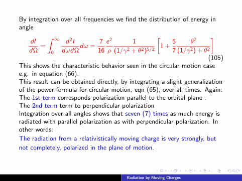
By integration over all frequencies we find the distribution of energy inangle

dI

dΩ=

∫ ∞0

d2I

dωdΩdω =

7

16

e2

ρ

1

(1/γ2 + θ2)5/2

[1 +

5

7

θ2

(1/γ2) + θ2

](105)

This shows the characteristic behavior seen in the circular motion casee.g. in equation (66).This result can be obtained directly, by integrating a slight generalizationof the power formula for circular motion, eqn (65), over all times. Again:The 1st term corresponds polarization parallel to the orbital plane .The 2nd term term to perpendicular polarizationIntegration over all angles shows that seven (7) times as much energy isradiated with parallel polarization as with perpendicular polarization. Inother words:

The radiation from a relativistically moving charge is very strongly, but

not completely, polarized in the plane of motion.


• The radiation is largely confined to the plane containing the motion,being more confined the higher the frequency relative to c/ρ.• If ω gets too large, then ξ will be large at all angles, and then therewill be negligible power emitted at those high frequencies.• The critical frequency beyond which there will be negligible totalenergy emitted at any angle can be defined by ξ = 1/2 and θ = 0(WHY?).Then we find

ωc =3

2γ3

(c

ρ

)=

3

2

(E

mc2

)3c

ρ(106)

this critical frequency agrees with the qualitative estimate (71).• If the motion is circular, then c/ρ is the fundamental frequency ofrotation, ω0.• The critical frequency is given by

ωc = ncω0 with harmonic number nc =3

2

(E

mc2

)3

(107)


For γ 1 the radiation is predominantly on the orbital plane and we canevaluate via eqn (104) the angular distribution for θ = 0.Thus for ω ωc we find

d2I

dωdΩ|θ=0 ≈

e2

c

[Γ(2/3)

π

]2(3

4

)1/3 (ωρc

)2/3

(108)

For ω ωc

d2I

dωdΩ|θ=0 ≈

3

4π

e2

cγ2 ω

ωce−ω/ωc (109)

These limiting case show that the spectrum at θ = 0 increases withfrequency roughly as ω2/3 well bellow the critical frequency, reaches amaximum in the neighborhood of ωc , and then drops exponentially to 0above that frequency.• The spread in angle at a fixed frequency can be estimated bydetermining the angle θc at which ξ(θc) ≈ ξ(0) + 1.• In the low frequency range (ω ωc), ξ(0) ≈ 0 so ξ(θc) ≈ 1 whichgives

θc ≈(

3c

ωρ

)1/3

=1

γ

(2ωc

ω

)1/3

(110)

We note that the low frequency components are emitted at much wider

angles than the average, 〈θ2〉1/2 ∼ γ−1.Radiation by Moving Charges

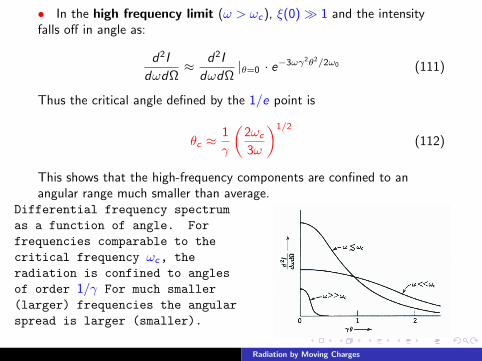
• In the high frequency limit (ω > ωc), ξ(0) 1 and the intensityfalls off in angle as:

d2I

dωdΩ≈ d2I

dωdΩ|θ=0 · e−3ωγ2θ2/2ω0 (111)

Thus the critical angle defined by the 1/e point is

θc ≈1

γ

(2ωc

3ω

)1/2

(112)

This shows that the high-frequency components are confined to anangular range much smaller than average.

Differential frequency spectrumas a function of angle. Forfrequencies comparable to thecritical frequency ωc, theradiation is confined to anglesof order 1/γ For much smaller(larger) frequencies the angularspread is larger (smaller).


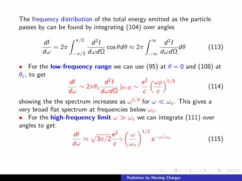
The frequency distribution of the total energy emitted as the particlepasses by can be found by integrating (104) over angles

dI

dω= 2π

∫ π/2

−π/2

d2I

dωdΩcos θdθ ≈ 2π

∫ ∞−∞

d2I

dωdΩdθ (113)

• For the low-frequency range we can use (95) at θ = 0 and (108) atθc , to get

dI

dω∼ 2πθc

d2I

dωdΩ|θ=0 ∼

e2

c

(ωρc

)1/3

(114)

showing the the spectrum increases as ω1/3 for ω ωc . This gives avery broad flat spectrum at frequencies below ωc .• For the high-frequency limit ω ωc we can integrate (111) overangles to get:

dI

dω≈√

3π/2e2

cγ

(ω

ωc

)1/2

e−ω/ωc (115)


A proper integration of over angles yields the expression,

dI

dω≈√

3e2

cγω

ωc

∫ ω

ω/ωc

K5/3(x)dx (116)

In the limit ω ωc , this reduces to the form (114) with numericalcoefficient 13/4, while for ω ωc it is equal to (115).• Bellow the behavior of dI/dω as function of the frequency

where y = ω/ωc and I = 4πe2γ4/3ρ.


The radiation represented by (104) and (116) is called synchrotronradiation because it was first observed in electron synchrotrons (1948).• For periodic circular motion the spectrum is actually discrete, beingcomposed of frequencies that are integral multipoles of the fundamentalfrequency ω0 = c/ρ.• Thus we should talk about the angular distribution of power radiatedin the nth multiple of ω0 instead of the energy radiated per unit frequencyinterval per passage of the particle. Thus we can write (WHY?)

dPn

dΩ=

1

2π

(c

ρ

)2d2I

dωdΩ|ω=nω0 (117)

Pn =1

2π

(c

ρ

)2dI

dω|ω=nω0 (118)

• These results have been compared with experiment at various energysynchrotrons. The angular, polarization and frequency distributions areall in good agreement with theory.

• Because of the broad frequency distribution shown in previous Figure,

covering the visible, ultraviolet and x-ray regions, synchrotron radiation is

a useful tool for studies in condensed matter and biology.


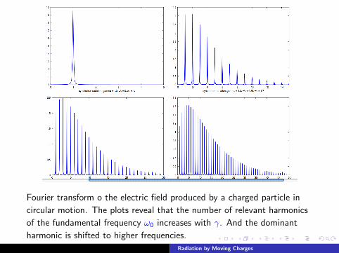
Fourier transform o the electric field produced by a charged particle in

circular motion. The plots reveal that the number of relevant harmonics

of the fundamental frequency ω0 increases with γ. And the dominant

harmonic is shifted to higher frequencies.


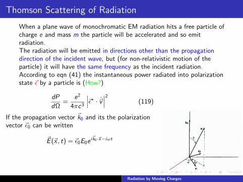
Thomson Scattering of Radiation

When a plane wave of monochromatic EM radiation hits a free particle ofcharge e and mass m the particle will be accelerated and so emitradiation.The radiation will be emitted in directions other than the propagationdirection of the incident wave, but (for non-relativistic motion of theparticle) it will have the same frequency as the incident radiation.According to eqn (41) the instantaneous power radiated into polarizationstate ~ε by a particle is (How?)

dP

dΩ=

e2

4πc3

∣∣∣~ε∗ · ~v ∣∣∣2 (119)

If the propagation vector ~k0 and its the polarizationvector ~ε0 can be written

~E (~x , t) = ~ε0E0ei~k0·~x−iωt


Then from the force eqn the acceleration will be

~v(t) = ~ε0e

mE0e

i~k0·~x−iωt (120)

Then the averaged power per unit solid angle can be expressed as

〈 dP

dΩ〉 =

c

8π|E0|2

(e2

mc2

)2

|~ε∗ · ~ε0|2 (121)

And since the phenomenon is practically scattering then it is convenientto used the scattering cross section as

dσ

dΩ=

Energy radiated/unit time/unit solid angle

Incident energy flux in energy/unit area/unit time(122)

Since the incident energy flux is the time averaging Poynting vector forthe plane wave i.e. c |E0|2/8π. Thus dividing with eqn (121) we get

dσ

dΩ=

(e2

mc2

)2

|~ε∗ · ~ε0|2 (123)


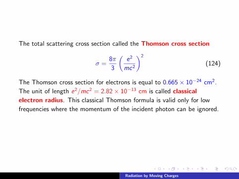
The total scattering cross section called the Thomson cross section

σ =8π

3

(e2

mc2

)2

(124)

The Thomson cross section for electrons is equal to 0.665× 10−24 cm2.

The unit of length e2/mc2 = 2.82× 10−13 cm is called classical

electron radius. This classical Thomson formula is valid only for low

frequencies where the momentum of the incident photon can be ignored.


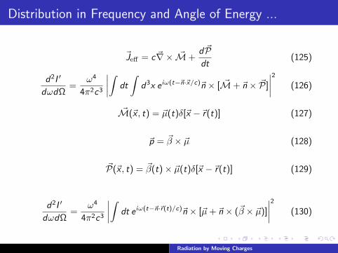
Distribution in Frequency and Angle of Energy ...

~Jeff = c ~∇× ~M+d ~Pdt

(125)

d2I ′

dωdΩ=

ω4

4π2c3

∣∣∣∣∫ dt

∫d3x e iω(t−~n·~x/c)~n × [ ~M+ ~n × ~P]

∣∣∣∣2 (126)

~M(~x , t) = ~µ(t)δ[~x −~r(t)] (127)

~p = ~β × ~µ (128)

~P(~x , t) = ~β(t)× ~µ(t)δ[~x −~r(t)] (129)

d2I ′

dωdΩ=

ω4

4π2c3

∣∣∣∣∫ dt e iω(t−~n·~r(t)/c)~n × [~µ+ ~n × (~β × ~µ)]

∣∣∣∣2 (130)


radiation by moving charges - institut by moving charges may 27, 20081 1j.d.jackson, "classical...

Documents