radar - oxford brookes university · ... fédération internationale de l’automobile ... 4-dof...
TRANSCRIPT

WWW.BROOKES.AC.UK/GO/RADAR
RADAR Research Archive and Digital Asset Repository
Copyright © and Moral Rights for this thesis are retained by the author and/or other copyright owners. A copy can be downloaded for personal non-commercial research or study, without prior permission or charge. This thesis cannot be reproduced or quoted extensively from without first obtaining permission in writing from the copyright holder(s). The content must not be changed in any way or sold commercially in any format or medium without the formal permission of the copyright holders.
Note if anything has been removed from thesis.
Images p1, 10, 14, 25, 26 and 38. Pages 289-294
When referring to this work, the full bibliographic details must be given as follows:
Pardo Barcelo, J. D. (2012) Optimisation of racing car suspensions featuring inerters. PhD Thesis. Oxford Brookes University.
Optimisation of Racing Car Suspensions featuring Inerters
by
Jose Daniel Pardo Barcelo
The Department of Mechanical Engineering and Mathematical
Sciences
Oxford Brookes University
A thesis submitted in partial fulfilment of the requirements of
Oxford Brookes University for the degree of
Doctor of Philosophy
November 2012


i
Acknowledgements
The research stage towards earning this PhD degree has been one of the most intellectually
inspiring experiences of my life. It has allowed me to grow as a person and as an engineer. I
would like to take this opportunity to thank the people who have helped me to get to the
finish line. First, I would like to thank my Director of Studies, Dr. James Balkwill, who has
played a key role in my success as a doctoral candidate. I am grateful for your support and
guidance throughout my PhD.
I would also like to thank the members of my supervisory committee: Dr. Denise Morrey and
Nick Bowler. I would like to give a very special thanks to Dr. Denise Morrey for your
invaluable help and active support in preparing and writing this thesis. Without your help,
insight, and guidance this work would not have been possible. I am thankful to Nick Bowler
for your feedback in the development of a lap-time simulator. I would also like to show my
deep appreciation to my research Tutors, Dr. Khaled Hayatleh and Dr. Rob Beale.
I would also like to thank all the members of the OBU Workshop, Kieron, Warwick and
Tony. I really appreciate all the effort and patience you put into having the test car built. I am
thankful to John and Ian who always assisted me with the logistics involved in my research.
To my fellow members of the MEMS Research Team: Luke Bennett, Tulay Ibicek, Marco
Cecotti, David Rodrigues and Dr. Nikos Vrellos. I would like to say thank you for all the
good moments we had together. I will always remember the important role you played in this
journey.
At this point, I would like to thank all of my close friends here: Santi, Dioni, Broja, Esteban,
Marte, Carlos Bravo, Silvia. Guys, you have always given me a huge moral support. You
always stood by my side in times of need and you celebrated my success.
Last but certainly not least, I would like to give an enormous “Thank you” to my parents,
Pepe and Africa, my brother, Nacho, and my Italian family, Nicola, Eliana, Simo. Even if we
are miles away, I always received your love and support as if you were next to me. Finally, I
would like to give a huge “Thank you” and a very big kiss to my girlfriend, Veronica. We
started this journey together and you have always given me the strength, support and love I
needed to complete it. We made it!
ii
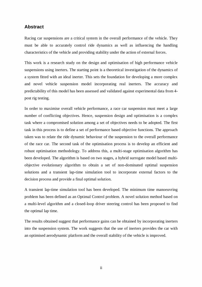
Abstract
Racing car suspensions are a critical system in the overall performance of the vehicle. They
must be able to accurately control ride dynamics as well as influencing the handling
characteristics of the vehicle and providing stability under the action of external forces.
This work is a research study on the design and optimisation of high performance vehicle
suspensions using inerters. The starting point is a theoretical investigation of the dynamics of
a system fitted with an ideal inerter. This sets the foundation for developing a more complex
and novel vehicle suspension model incorporating real inerters. The accuracy and
predictability of this model has been assessed and validated against experimental data from 4-
post rig testing.
In order to maximise overall vehicle performance, a race car suspension must meet a large
number of conflicting objectives. Hence, suspension design and optimisation is a complex
task where a compromised solution among a set of objectives needs to be adopted. The first
task in this process is to define a set of performance based objective functions. The approach
taken was to relate the ride dynamic behaviour of the suspension to the overall performance
of the race car. The second task of the optimisation process is to develop an efficient and
robust optimisation methodology. To address this, a multi-stage optimisation algorithm has
been developed. The algorithm is based on two stages, a hybrid surrogate model based multi-
objective evolutionary algorithm to obtain a set of non-dominated optimal suspension
solutions and a transient lap-time simulation tool to incorporate external factors to the
decision process and provide a final optimal solution.
A transient lap-time simulation tool has been developed. The minimum time manoeuvring
problem has been defined as an Optimal Control problem. A novel solution method based on
a multi-level algorithm and a closed-loop driver steering control has been proposed to find
the optimal lap time.
The results obtained suggest that performance gains can be obtained by incorporating inerters
into the suspension system. The work suggests that the use of inerters provides the car with
an optimised aerodynamic platform and the overall stability of the vehicle is improved.

iii
Nomenclature
OBU – Oxford Brookes University
FE – Finite Element
F1 – Formula One
FiA – Fédération Internationale de l’Automobile
PMEM – Permanent Magnet Electric Motor
CAD – Computer-Aided Design
ANN – Artificial Neural Network
CFD – Computational Fluid Dynamics
MIMO – Multiple Input, Multiple Output
3D – Three Dimensional
2D – Two Dimensional
EOM – Equations of Motion
CPU – Central Processing Unit
MOO – Multi-Objective Optimization
MOOP – Multi-Objective Optimization Problem
SQP – Sequential Quadratic Programming
LMI – Linear Matrix Inequality
LMIP – Linear Matrix Inequality Problem
EA – Evolutionary Algorithm
MOEA – Multi-Objective Evolutionary Algorithm
GA – Genetic Algorithm
PSA – Pattern Search Algorithm
iv
NSGA-II – Fast Non-Dominated Sorting Genetic Algorithm
DOF – Degree of Freedom
SDOF – Single-Degree-Of-Freedom
n-DOF – n-Degree-Of-Freedom
DACE – Design and Analysis of Computer Experiments
DoE – Design of Experiments
OA – Orthogonal Array
LHS – Latin Hypercube Sampling
PR – Polynomial Regression
KRG – Kriging model
RBF – Radial Basis Functions
MAE – Maximum Absolute Error
AAE – Average Absolute Error
RMSE – Root Mean Square Error
HBVP – Hamiltonian Boundary-Value Problem
MBD – Multi-Body Dynamics
IR – Installation Ratio
CPV – Constant Peak Velocity
FRF – Frequency Response Function
SISO – Single-Input, Single-Output
LSB – Low-Speed Bump
HSB – High-Speed Bump
LSR – Low-Speed Rebound

v
HSR – High-Speed Rebound
FWM – Flywheel Mount
LTS – Lap-time Simulation
QSS – Quasi Steady-State
OC – Optimal Control
RHC – Receding Horizon Control
MPC – Model Predictive Control
RWD – Rear Wheel Drive
CoG – Centre of Gravity
MTM – Minimum Time Manoeuvring
MLOA – Multilevel Optimisation Algorithm
IWN – Integrated White Noise

vi
List of Figures
Figure 1-1: 1992 FW14B Williams Formula 1 car equipped with fully active suspension ...... 1
Figure 1-2: Prototype inerter designed at Cambridge University (Smith, 2003) ..................... 2
Figure 2-1: Mechanical – Electrical analogy: Classical (upper) and Revised with inerter
(lower) (Smith, 2002) .......................................................................................................... 10
Figure 2-2: Quarter-Car test rig (Andersen, 2007) ............................................................... 14
Figure 2-3: Process of MOO using Surrogate Approximations (Wilson, et al., 2001) ........... 25
Figure 2-4: Techniques for Metamodelling (Simpson, et al., 2001) ...................................... 26
Figure 2-5: 3-DOF Bicycle Model ....................................................................................... 33
Figure 3-1: Conceptual design of a ball screw inerter (Smith, 2006) .................................... 38
Figure 3-2: Un-damped SDOF system with inerter .............................................................. 40
Figure 3-3: Steady-state response of an un-damped SDOF system. Amplitude ratio response
(upper graph) and phase response (lower graph) .................................................................. 43
Figure 3-4: Damped SDOF system with inerter ................................................................... 45
Figure 3-5: Steady-state response of damped SDOF system (Damping Ratio = 0.1).
Amplitude ratio response (upper graph) and phase response (lower graph) .......................... 47
Figure 3-6: Steady-state response of damped SDOF system (Damping Ratio = 0.5).
Amplitude ratio response (upper graph) and phase response (lower graph) .......................... 48
Figure 3-7: Steady-state response of damped SDOF system (Damping Ratio = 1). Amplitude
ratio response (upper graph) and phase response (lower graph) ........................................... 48
Figure 3-8: Transient response of the system in the under-damped region ........................... 53
Figure 3-9: Transient response of the system in the transition region ................................... 54
Figure 3-10: Study of damping ratio sensitivity against damping coefficient and inertance .. 56
Figure 4-1: Generic mechanical design process ................................................................... 59

vii
Figure 4-2: Specific design process of a physical inerter...................................................... 61
Figure 4-3: Detailed 3D CAD design of a ball-screw inerter ................................................ 66
Figure 4-4: Photograph of a prototype inerter: a) Inerter assembly and b) Principal
components ......................................................................................................................... 66
Figure 4-5: 3D MBD kinematic model of re-designed front suspension ............................... 68
Figure 4-6: 3D MBD kinematic model of re-designed rear suspension ................................ 69
Figure 4-7: 3D CAD design of the new test car ................................................................... 72
Figure 4-8: 3D CAD detailed design of the new front suspension incorporating inerter ....... 72
Figure 4-9: 3D CAD detailed design of the new rear suspension incorporating inerter ......... 73
Figure 4-10: General view of the redesigned test vehicle ..................................................... 74
Figure 4-11: Test car front suspension view ........................................................................ 74
Figure 4-12: Test car rear suspension view .......................................................................... 75
Figure 4-13: Upper view of OBU Four-post rig test facility ................................................. 76
Figure 4-14: Lower view of OBU Four-post rig test facility ................................................ 76
Figure 4-15: Schematic representation of 4-post rig ............................................................. 77
Figure 4-16: Transducer interface box ................................................................................. 78
Figure 4-17: Four-post rig main command window ............................................................. 79
Figure 4-18: Simplified 7-DOF vehicle suspension model (Bennett, 2012) .......................... 82
Figure 4-19: Front body accelerometer location................................................................... 84
Figure 4-20: Rear body accelerometer location .................................................................... 85
Figure 4-21: Front hub accelerometer position .................................................................... 85
Figure 4-22: Rear hub accelerometer position...................................................................... 86
Figure 4-23: Front strut displacement potentiometer position .............................................. 87
viii
Figure 4-24: Rear strut displacement potentiometer location ............................................... 87
Figure 4-25: Four-post rig weight setting procedure ............................................................ 88
Figure 4-26: Installation ratio test input wave ...................................................................... 89
Figure 4-27: Actuator displacement vs Suspension displacement – IR measurement ........... 90
Figure 4-28: Experimental unsprung mass estimation: experimental data (upper) and linear
regression (lower) ............................................................................................................... 91
Figure 4-29: Example of race track vertical profile: actual profile (upper) and PSD
representation (lower) ......................................................................................................... 92
Figure 4-30: PSD of race track elevation profile for a vehicle travelling at 90 m/s ............... 94
Figure 4-31: Example of rig test swept sine input – displacement (upper), velocity (middle)
and acceleration (lower) ...................................................................................................... 95
Figure 4-32: Parameter Estimation command window ......................................................... 97
Figure 4-33: Current parameter estimation program suspension model – No inerters (Bennett,
2012) .................................................................................................................................. 98
Figure 4-34: Suspension layout with real inerters .............................................................. 100
Figure 4-35: Estimated tyre stiffness versus tyre deflection from a suspension with and
without inerters ................................................................................................................. 102
Figure 5-1: 4-DOF Half Car model................................................................................... 106
Figure 5-2: 3-DOF Vehicle suspension model (Graf & Kosuch, 2008) .............................. 111
Figure 5-3: 7-DOF Full-car suspension model (Bennett, 2012) .......................................... 111
Figure 5-4: Dynamic apparent mass comparison – experimental data and 7-DOF model ... 113
Figure 5-5: Front CPL/Input Acceleration frequency response .......................................... 114
Figure 5-6: Rear CPL/Input Acceleration frequency response............................................ 114
Figure 5-7: SISO system ................................................................................................... 117

ix
Figure 5-8: Suspension layout featuring with ideal mechanical elements – Type 1 ............ 118
Figure 5-9: Dynamic suspension stiffness comparison: experimental rig data vs. suspension
type 1 ................................................................................................................................ 119
Figure 5-10: Front CPL frequency response: experimental vs. simulation type 1 ............... 120
Figure 5-11: Rear CPL frequency response: experimental vs. simulation type 1 ................ 120
Figure 5-12: Discrete spring and dashpot model (Allen, et al., 2006) ................................. 121
Figure 5-13: Nonlinear experimental inerter model (Wang & Su, 2008) ............................ 122
Figure 5-14: Linearised experimental inerter model........................................................... 122
Figure 5-15: Effect of installation stiffness - Dynamic Stiffness frequency response.......... 124
Figure 5-16: Effect of installation stiffness - CPL/Static mass frequency response............. 124
Figure 5-17: Effect of installation stiffness - Body Acceleration/Input Acceleration frequency
response ............................................................................................................................ 125
Figure 5-18: Effect of installation stiffness - Unsprung Acceleration/Input Acceleration
frequency response ............................................................................................................ 125
Figure 5-19: Body Acceleration response of 2-DOF system in ki= 100 N/mm – Damping ratio
comparison........................................................................................................................ 126
Figure 5-20: CPL response of 2-DOF system in ki= 100 N/mm – Damping ratio comparison
......................................................................................................................................... 127
Figure 5-21: Suspension model layout type 2 .................................................................... 127
Figure 5-22: Dynamic suspension stiffness comparison: experimental rig data vs. suspension
layout type 2 ..................................................................................................................... 128
Figure 5-23: Front CPL frequency response: experimental vs. simulation type 2 ............... 129
Figure 5-24: Rear CPL frequency response: experimental vs. simulation type 2 ................ 129
Figure 5-25: Front Tyre Stiffness and Damping comparison – Experimental data vs. linear
tyre model ......................................................................................................................... 131
x
Figure 5-26: Rear Tyre Stiffness and Damping comparison – Experimental data vs. linear tyre
model ................................................................................................................................ 131
Figure 5-27: Tyre elastic properties – Tyre model comparison .......................................... 132
Figure 5-28: Front CPL ratio dynamic response with linear tyre mode .............................. 133
Figure 5-29: Absolute tyre deflection dynamic response at various input amplitudes ......... 134
Figure 5-30: Experimental dynamic stiffness response for various input amplitudes .......... 135
Figure 5-31: Nonlinear experimental tyre stiffness characteristic: Front (upper) and rear
(lower) .............................................................................................................................. 136
Figure 5-32: Nonlinear experimental tyre damping characteristic: Front (upper) and rear
(lower) .............................................................................................................................. 137
Figure 5-33: Nonlinear tyre stiffness model comparison between experimental vs.
exponential model ............................................................................................................. 138
Figure 5-34: Nonlinear tyre damping model comparison between experimental vs.
exponential model ............................................................................................................. 139
Figure 5-35: Front CPL ratio frequency response with nonlinear tyre model ..................... 140
Figure 5-36: Rear CPL frequency ratio response with nonlinear tyre model....................... 140
Figure 5-37: Front unsprung mass acceleration ratio frequency response with nonlinear tyre
model ................................................................................................................................ 141
Figure 5-38: Front unsprung mass acceleration ratio frequency response with nonlinear tyre
model ................................................................................................................................ 141
Figure 5-39: Dynamic stiffness frequency response Setup 1: front (upper) and rear (lower)146
Figure 5-40: Front Body Acceleration Ratio frequency response – Setup 1 ........................ 147
Figure 5-41: Rear Body Acceleration Ratio frequency response – Setup 1 ......................... 147
Figure 5-42: Front CPL ratio frequency response – Setup 1 ............................................... 148
Figure 5-43: Rear CPL ratio frequency response – Setup 1 ................................................ 148

xi
Figure 5-44: Front unsprung mass acceleration ratio frequency response – Setup 1 ........... 149
Figure 5-45: Front unsprung mass acceleration ratio frequency response – Setup 1 ........... 149
Figure 5-46: Pitch acceleration ratio frequency response – Setup 1 .................................... 150
Figure 5-47: Dynamic stiffness frequency response Setup 2: front (upper) and rear (lower)151
Figure 5-48: Front Body Acceleration Ratio frequency response – Setup 2 ........................ 152
Figure 5-49: Rear Body Acceleration Ratio frequency response – Setup 2 ......................... 152
Figure 5-50: Front CPL ratio frequency response – Setup 2 ............................................... 153
Figure 5-51: Rear CPL ratio frequency response – Setup 2 ................................................ 153
Figure 5-52: Front unsprung mass acceleration ratio frequency response – Setup 2 ........... 154
Figure 5-53: Rear unsprung mass acceleration ratio frequency response – Setup 2 ............ 154
Figure 5-54: Pitch acceleration ratio frequency response – Setup 2 .................................... 155
Figure 5-55: Dynamic stiffness frequency response Setup 3: front (upper) and rear (lower)156
Figure 5-56: Front Body Acceleration Ratio frequency response – Setup 3 ........................ 157
Figure 5-57: Rear Body Acceleration Ratio frequency response – Setup 3 ......................... 157
Figure 5-58: Front CPL ratio frequency response – Setup 3 ............................................... 158
Figure 5-59: Rear CPL ratio frequency response – Setup 3 ................................................ 158
Figure 5-60: Front unsprung mass acceleration ratio frequency response – Setup 3 ........... 159
Figure 5-61: Rear unsprung mass acceleration ratio frequency response – Setup 3 ............ 159
Figure 5-62: Pitch acceleration ratio frequency response – Setup 3 .................................... 160
Figure 5-63: Dynamic stiffness frequency response Setup 4: front (upper) and rear (lower)161
Figure 5-64: Front Body Acceleration Ratio frequency response – Setup 4 ........................ 161
Figure 5-65: Rear Body Acceleration Ratio frequency response – Setup 4 ......................... 162
Figure 5-66: Front CPL ratio frequency response – Setup 4 ............................................... 162
xii
Figure 5-67: Rear CPL ratio frequency response – Setup 4 ................................................ 163
Figure 5-68: Front unsprung mass acceleration ratio frequency response – Setup 4 ........... 163
Figure 5-69: Rear unsprung mass acceleration ratio frequency response – Setup 4 ............ 164
Figure 5-70: Pitch acceleration ratio frequency response – Setup 4 .................................... 164
Figure 5-71: Dynamic stiffness frequency response Setup 5: front (upper) and rear (lower)165
Figure 5-72: Front Body Acceleration Ratio frequency response – Setup 5 ........................ 166
Figure 5-73: Rear Body Acceleration Ratio frequency response – Setup 5 ......................... 166
Figure 5-74: Front CPL ratio frequency response – Setup 5 ............................................... 167
Figure 5-75: Rear CPL ratio frequency response – Setup 5 ................................................ 167
Figure 5-76: Front unsprung mass acceleration ratio frequency response – Setup 5 ........... 168
Figure 5-77: Rear unsprung mass acceleration ratio frequency response – Setup 5 ............ 168
Figure 5-78: Pitch acceleration ratio frequency response – Setup 5 .................................... 169
Figure 5-79: Front CPL response – Mechanical grip optimisation...................................... 173
Figure 5-80: Rear CPL response – Mechanical grip optimisation ....................................... 173
Figure 5-81: Front Ride Height response – Mechanical grip optimisation .......................... 174
Figure 5-82: Rear Ride Height response – Mechanical grip optimisation ........................... 174
Figure 5-83: Front CPL response – Aero grip optimisation ................................................ 176
Figure 5-84: Rear CPL response – Aero grip optimisation ................................................. 176
Figure 5-85: Front Ride Height response – Aero grip optimisation .................................... 177
Figure 5-86: Rear Ride Height response – Aero grip optimisation ..................................... 177
Figure 5-87: Tyre stiffness characteristic comparison – Front (upper) and rear (lower) ...... 181
Figure 5-88: Effect of unsprung mass variation in dynamic CPL response ......................... 182
Figure 6-1: Overall Vehicle Model – Modular Modelling .................................................. 187
xiii
Figure 6-2: Modular Modelling operational approach ........................................................ 187
Figure 6-3: Sprung Single Track Vehicle Model: Plan view (upper) and lateral view (lower)
......................................................................................................................................... 189
Figure 6-4: Powertrain layout ............................................................................................ 191
Figure 6-5: Engine map ..................................................................................................... 192
Figure 6-6: Tyre lateral force characteristic curve .............................................................. 194
Figure 6-7: Lateral force variation due to vertical load variation: transient vs. steady-state 195
Figure 6-8: Aerodynamic maps ......................................................................................... 197
Figure 6-9: Track map definition (Casanova, 2000) ........................................................... 198
Figure 6-10: Lap-time simulator driver model ................................................................... 199
Figure 6-11: Steering driver model (Casanova, 2000) ........................................................ 200
Figure 6-12: Nonlinear path preview steering control scheme (Casanova, 2000)................ 201
Figure 6-13: Race track discretisation (Braghin, et al., 2008) ............................................. 206
Figure 6-14: Shortest Path racing trajectory ....................................................................... 208
Figure 6-15: Minimum Curvature racing trajectory ........................................................... 209
Figure 6-16: Variable control input discretisation scheme ................................................. 211
Figure 6-17: Race track - crossing point sections ............................................................... 213
Figure 6-18: Initial vehicle speed profile estimation .......................................................... 214
Figure 6-19: Initial control input guess diagram ................................................................ 215
Figure 6-20: Estimated control input initial guess .............................................................. 216
Figure 6-21: Estimated vs. Real vehicle speed profile ........................................................ 217
Figure 6-22: Estimated initial guess trajectory ................................................................... 217
Figure 6-23: Bahrain GP track sections ............................................................................. 219
xiv
Figure 6-24: Bahrain Example: Control input histories ...................................................... 223
Figure 6-25: Bahrain Example: Optimal trajectory ............................................................ 223
Figure 6-26: Bahrain Example: Forward speed profile and gear change history ................. 224
Figure 6-27: Bahrain Example: Front and rear slip angle histories ..................................... 224
Figure 6-28: Bahrain Example: Front and rear slip ratio histories ...................................... 225
Figure 6-29: Bahrain Example: Ride Height and Pitch attitude histories ............................ 225
Figure 6-30: Bahrain Example: Aerodynamic Lift and F/R Distribution histories .............. 226
Figure 6-31: Bahrain Example: g-g-V Diagram ................................................................. 226
Figure 6-32: Bahrain Example: Front and rear vertical tyre load histories .......................... 227
Figure 6-33: Bahrain Example: Contact patch load variation frequency response .............. 227
Figure 7-1: SDOF Body Displacement Amplitude Ratio for different k values .................. 232
Figure 7-2: Effect of suspension stiffness in the RMS of Body Displacement Amplitude Ratio
......................................................................................................................................... 233
Figure 7-3: Effect of vertical load on cornering performance (Gillespie, 1992) .................. 235
Figure 7-4: Integrated white noise track profile signal ....................................................... 237
Figure 7-5: Modal Weighting factor .................................................................................. 238
Figure 7-6: Effect of aerodynamics in the cornering performance of a race car (Dominy,
1992) ................................................................................................................................ 240
Figure 7-7: Understeering characteristic under different road surfaces (Mashadi & Crolla,
2005) ................................................................................................................................ 242
Figure 7-8: Proposed suspension optimisation process layout ............................................ 244
Figure 7-9: Optimisation cost function evaluation through actual dynamic model (upper) and
surrogate model (lower) .................................................................................................... 246
xv
Figure 7-10: Evaluation of the performance of the metamodel in predicting cost function J1
......................................................................................................................................... 248
Figure 7-11: Evaluation of the performance of the metamodel in predicting cost function J2
......................................................................................................................................... 249
Figure 7-12: Error analysis for estimation of J1 (upper) and J2 (lower) ............................... 249
Figure 7-13: Cost function comparison between metamodel and original vehicle suspension
model ................................................................................................................................ 252
Figure 7-14: Decision Making Process .............................................................................. 255
Figure 7-15: Suspension multiobjective optimisation results – 3D Plot .............................. 259
Figure 7-16: Suspension multiobjective optimisation results – 2D plots ............................ 260
Figure 7-17: Clustered results for MO results – Conventional suspension .......................... 261
Figure 7-18: Clustered results for MO results – Suspension featuring inerters ................... 262
Figure 7-19: Difference in load sensitivity around ............................................................. 264
Figure 7-20: Race car trajectory for different suspension layouts at Turn 4 ........................ 265
Figure 7-21: Race car speed trace for different suspension layouts at Turn 4 ..................... 265
Figure B-1: Schematic plan view of vehicle model for lap-time simulation.........................295
Figure B-2: Schematic lateral view of vehicle model for lap-time simulation......................295

xvi
List of Tables
Table 3-1: Mechanical properties of the un-damped SDOF system ...................................... 42
Table 3-2: Mechanical properties of the damped SDOF system ........................................... 47
Table 3-3: Initial conditions for transient analysis ............................................................... 53
Table 3-4: Damping coefficients used in simulation ............................................................ 53
Table 3-5: Results of the transient response with c = 1000 Ns/m ......................................... 54
Table 3-6: Results of the transient response with c = 3465 Ns/m ......................................... 55
Table 3-7: Parameters used for sensitivity analysis .............................................................. 55
Table 4-1: Decision matrix for physical inerter design solutions .......................................... 63
Table 4-2: Ball-screw mechanism design requirements ....................................................... 65
Table 4-3: Ball-screw mechanism specfications .................................................................. 65
Table 4-4: Range of adjustability of ball-screw inerter......................................................... 65
Table 4-5: Colour-coded key table for MBD suspension models ......................................... 69
Table 4-6: Spring Stiffness design matrix for rear suspension .............................................. 71
Table 4-7: Summary of test inputs used in experimental testing ........................................... 96
Table 5-1: Input parameters for Half-car 4-DOF model study ............................................ 107
Table 5-2: Decision matrix for selection of simulation software ........................................ 108
Table 5-3: Simulation time comparison – Full-car and Half-car models ............................. 116
Table 5-4: Vehicle data for installation stiffness study ....................................................... 123
Table 5-5: Tyre properties for linear tyre model study ....................................................... 132
Table 5-6: Estimated parameters for tyre model ................................................................ 138
Table 5-7: Vehicle data properties used in validation process ............................................ 142
Table 5-8: Tyre elastic properties used in validation process ............................................. 143

xvii
Table 5-9: General suspension settings .............................................................................. 144
Table 5-10: Summary of inerter settings tested .................................................................. 144
Table 5-11: Estimated suspension parameters – Setup 1 .................................................... 145
Table 5-12: Estimated suspension parameters – Setup 2 .................................................... 150
Table 5-13: Estimated suspension parameters – Setup 3 .................................................... 155
Table 5-14: Estimated suspension parameters – Setup 4 .................................................... 160
Table 5-15: Estimated suspension parameters – Setup 5 .................................................... 165
Table 5-16: Design space range – Suspension optimisation validation ............................... 171
Table 5-17: Optimised suspension parameters for J1 - Mechanical grip suspension
optimisation validation ...................................................................................................... 172
Table 5-18: Summary of mechanical grip objective function results .................................. 172
Table 5-19: Optimised suspension parameters – Aero grip suspension optimisation validation
......................................................................................................................................... 175
Table 5-20: Summary of aero grip objective function results ............................................. 175
Table 5-21: Summary of validation errors ......................................................................... 179
Table 5-22: Hub acceleration average errors – Frequency range 0.5-20 Hz ........................ 180
Table 6-1: Summary of optimisation parameters – Bahrain example ................................. 220
Table 6-2: Bahrain GP track main characteristics .............................................................. 221
Table 6-3: Summary of lap-time optimisation.................................................................... 221
Table 7-1: Definition of Initial Design Space .................................................................... 231
Table 7-2: Definition of Final Design Space ...................................................................... 234
Table 7-3: Analysis of accuracy of Kriging metamodel for each cost function ................... 250
Table 7-4: Summary of computational time of original and metamodel for batch simulation
......................................................................................................................................... 251

xviii
Table 7-5: Summary of computational time of original and metamodel for optimisation ... 252
Table 7-6: Limits of the optimisation design space ............................................................ 256
Table 7-7: Limits of the DoE space ................................................................................... 257
Table 7-8: MOEA setting parameters ................................................................................ 257
Table 7-9: Summary of clustered optimised suspension settings – Conventional suspension
......................................................................................................................................... 261
Table 7-10: Summary of clustered optimised suspension settings – Suspension featuring
inerters .............................................................................................................................. 262
Table 7-11: Summary of lap times for both suspension layouts ......................................... 263

xix
Table of Contents
Acknowledgements ............................................................................................................... i
Abstract ............................................................................................................................... ii
Nomenclature ..................................................................................................................... iii
List of Figures..................................................................................................................... vi
List of Tables .................................................................................................................... xvi
Table of Contents ............................................................................................................. xix
1. Introduction ................................................................................................................. 1
1.1. Introduction ............................................................................................................ 1
1.2. Aims of the Research .............................................................................................. 4
1.3. Thesis Outline ......................................................................................................... 5
2. Literature Review ........................................................................................................ 7
2.1. Introduction ............................................................................................................ 7
2.2. Race Car Suspension Historical Background ........................................................... 8
2.3. Inerter Technology .................................................................................................. 9
2.3.1. Physical realisation of Inerters ....................................................................... 10
2.3.2. Inerter Technology applied to Vehicle Suspension Dynamics......................... 11
2.3.3. Inerter Technology applied to other Engineering fields .................................. 12
2.4. Experimental Testing on Vehicle Suspensions ...................................................... 13
2.5. Virtual Suspension Simulation .............................................................................. 15
2.5.1. Modelling of vehicle equations of motion ...................................................... 16
2.5.2. Modelling of individual suspension components ............................................ 17
2.6. Suspension Optimisation ....................................................................................... 18

xx
2.6.1. Performance Objective Functions for Suspension Systems ............................. 19
2.6.2. Multi-objective Optimisation Algorithm ........................................................ 21
2.6.3. Surrogate Model Based Optimisation ............................................................. 23
2.7. Lap-Time Simulation ............................................................................................ 27
2.7.1. Previous work on Transient Lap-Time Simulation.......................................... 28
2.7.2. Lap Time Simulation as an Optimal Control Problem .................................... 29
2.7.3. Full Vehicle Model ........................................................................................ 31
2.7.4. Lap Time Simulation as part of Suspension Optimisation Algorithm .............. 34
2.8. Summary .............................................................................................................. 35
3. Theoretical Analysis of Ideal Inerters in Vibratory Systems ................................... 37
3.1. Introduction .......................................................................................................... 37
3.2. Definition of the properties of an ideal inerter ....................................................... 38
3.3. Analysis of an un-damped Inerter modelled as a SDOF ......................................... 39
3.4. Analysis of a Damped Inerter modelled as a SDOF ............................................... 45
3.4.1. Analysis in the frequency domain .................................................................. 46
3.4.2. Analysis in the time domain ........................................................................... 50
3.4.3. Study of sensitivity ........................................................................................ 55
3.5. Summary .............................................................................................................. 57
4. Experimental Design ................................................................................................. 59
4.1. Introduction .......................................................................................................... 59
4.2. Design of Racing Car Suspension incorporating Real Inerters ............................... 60
4.2.1. Design of a Mechanical Inerter ...................................................................... 61
4.2.2. Design of a prototype test car ......................................................................... 66

xxi
4.3. Experimental Test System Description .................................................................. 75
4.4. System calibration Procedure ................................................................................ 80
4.5. Parameter Determination Method .......................................................................... 81
4.5.1. Set of parameters required .............................................................................. 81
4.5.2. Vehicle Instrumentation Procedure ................................................................ 83
4.5.3. Four-Post Rig Operation Procedure ................................................................ 88
4.5.4. Frequency Analysis and Parameter Estimation Software ................................ 96
4.5.5. Extensions of current parameter estimation method ........................................ 98
4.6. Summary ............................................................................................................ 104
5. Vehicle Suspension Modelling and Validation ....................................................... 105
5.1. Introduction ........................................................................................................ 105
5.2. Selection of the most suitable Modelling Software .............................................. 106
5.3. Selection of the most suitable Model Complexity ................................................ 109
5.3.1. Vehicle suspension model complexity for Parameter Estimation .................. 110
5.3.2. Vehicle suspension model for Optimisation ................................................. 115
5.4. Modelling Suspension System Features ............................................................... 116
5.4.1. Suspension System Layout featuring Inerters ............................................... 118
5.4.2. Non-linear Vertical Tyre Modelling ............................................................. 130
5.5. Suspension Validation with 4-Post Rig Test Experimental Results ...................... 142
5.5.1. Analysis of model accuracy for different inerter settings .............................. 143
5.5.2. Analysis of model predictability via suspension optimisation ....................... 170
5.5.3. Analysis of correlation errors ....................................................................... 178
5.6. Summary ............................................................................................................ 184
xxii
6. Lap-Time Simulation .............................................................................................. 185
6.1. Introduction ........................................................................................................ 185
6.2. Full-vehicle Dynamic Equations of Motion ......................................................... 186
6.2.1. Vehicle and Wheel Dynamics Model ........................................................... 188
6.2.2. Powertrain/Brake System Model .................................................................. 190
6.2.3. Tyre Model .................................................................................................. 193
6.2.4. Aerodynamic model ..................................................................................... 196
6.2.5. Suspension Model ........................................................................................ 198
6.2.6. Track Model ................................................................................................ 198
6.2.7. Driver Model ............................................................................................... 199
6.3. Minimum Time Manoeuvre - Problem Statement ................................................ 202
6.3.1. Independent variable transformation ............................................................ 203
6.3.2. Definition of the minimum lap-time cost function ........................................ 204
6.4. Multilevel optimisation algorithm - Solution Method .......................................... 204
6.4.1. MLOA level 1: Trajectory Planning ............................................................. 206
6.4.2. MLOA level 2: Lap Time Minimisation ....................................................... 210
6.4.3. Discretisation Scheme .................................................................................. 210
6.4.4. Initial Guess Algorithm ................................................................................ 213
6.5. Case Study .......................................................................................................... 218
6.5.1. Optimal Time Manoeuvring problem set-up ................................................. 218
6.5.2. Bahrain GP Circuit – Results ....................................................................... 221
6.6. Summary ............................................................................................................ 228
7. Suspension Performance Optimization .................................................................. 229

xxiii
7.1. Introduction ........................................................................................................ 229
7.2. Definition of the Multi-Objective Suspension Optimisation Problem................... 230
7.3. Definition of the Design Space ............................................................................ 230
7.4. Definition of Optimisation Evaluation Criteria .................................................... 234
7.4.1. Mechanical Grip Cost Function .................................................................... 234
7.4.2. Aerodynamic Grip Cost Function ................................................................. 239
7.4.3. Mechanical balance Cost Function ............................................................... 241
7.5. Development of the Optimization Methodology .................................................. 243
7.5.1. Surrogate Modelling using Kriging Method ................................................. 245
7.5.2. Multi-Objective Algorithm........................................................................... 252
7.5.3. Decision Making Process via the use of Lap-time simulation ....................... 254
7.6. Case Study .......................................................................................................... 255
7.6.1. Optimisation Process Set-up......................................................................... 255
7.6.2. Optimisation results and discussions ............................................................ 258
7.7. Summary ............................................................................................................ 266
8. Conclusions and Future Work ................................................................................ 267
8.1. Summary of the Objectives Achieved.................................................................. 267
8.2. Recommendations for future work ...................................................................... 269
References........................................................................................................................ 272
Appendix A: OBU Four-post rig Calibration Certificate .............................................. 288
Appendix B: Derivation of Vehicle Equations of Motion .............................................. 295

Optimisation of racing car suspensions featuring inerters
1
1. Introduction
1.1. Introduction
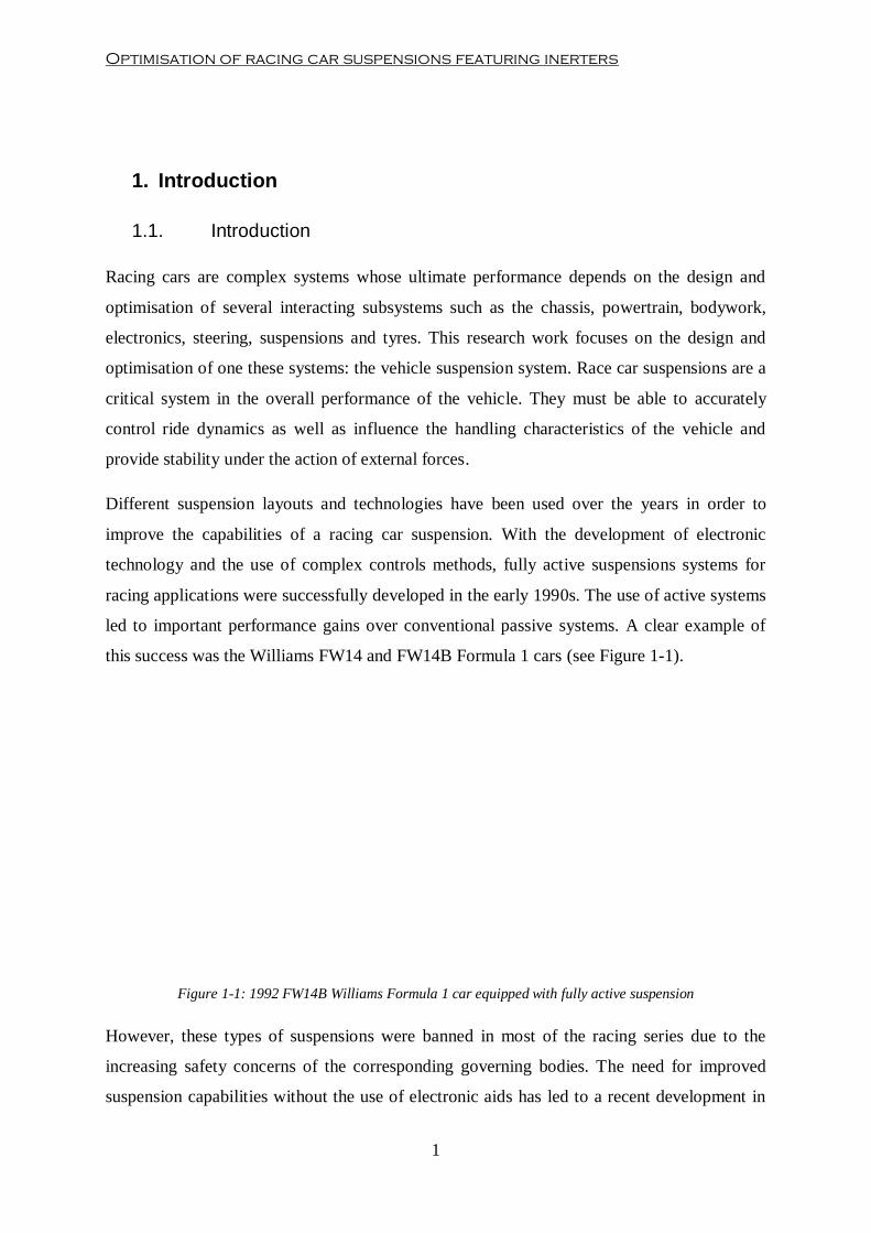
Racing cars are complex systems whose ultimate performance depends on the design and
optimisation of several interacting subsystems such as the chassis, powertrain, bodywork,
electronics, steering, suspensions and tyres. This research work focuses on the design and
optimisation of one these systems: the vehicle suspension system. Race car suspensions are a
critical system in the overall performance of the vehicle. They must be able to accurately
control ride dynamics as well as influence the handling characteristics of the vehicle and
provide stability under the action of external forces.
Different suspension layouts and technologies have been used over the years in order to
improve the capabilities of a racing car suspension. With the development of electronic
technology and the use of complex controls methods, fully active suspensions systems for
racing applications were successfully developed in the early 1990s. The use of active systems
led to important performance gains over conventional passive systems. A clear example of
this success was the Williams FW14 and FW14B Formula 1 cars (see Figure 1-1).
Figure 1-1: 1992 FW14B Williams Formula 1 car equipped with fully active suspension
However, these types of suspensions were banned in most of the racing series due to the
increasing safety concerns of the corresponding governing bodies. The need for improved
suspension capabilities without the use of electronic aids has led to a recent development in

Chapter 1- Introduction
2
passive suspension technology. Dr. Malcolm C. Smith (2002) introduced a new passive
mechanical device that could have potential performance benefits in passive vehicle
suspensions, called an inertial damper, or as it is most commonly known nowadays, an
inerter. An ideal inerter was defined as a massless linear two-terminal, one-port device in
which the force applied to the terminals is proportional to the relative acceleration between
these terminals (Smith, 2002). The first physical prototype inerter reported in literature was
created at Cambridge University (Figure 1-2).
Figure 1-2: Prototype inerter designed at Cambridge University (Smith, 2003)
According to this work (Smith, 2002), inerters could be used to create suspension layouts that
could potentially provide enhanced suspension capabilities. In theoretical work presented in
literature (Smith & Wang, 2004), the introduction of inerters into the suspension required all
suspension components to be tuned appropriately if performance benefits are to be obtained.
Moreover, in order to design a winning race car, all of the systems must be designed to
maximise the performance of the vehicle. In the particular case of the suspension system, the
main functions or goals that a racing car suspension must achieve in order to optimise vehicle
performance are:
Optimisation of racing car suspensions featuring inerters
3
To keep the tyres in contact with race track.
To resist the chassis motions induced by external forces (inertial and aerodynamic
forces).
To control the handling characteristics of the vehicle in dynamic situations.
All these suspension objective functions need to be optimised simultaneously if race car
performance is to be maximised. Multi-objective optimisation algorithms allow designers to
find optimal suspension solutions considering all of the defined objective functions
simultaneously. However, the fact that some objectives may conflict with each other prevents
from obtaining a unique optimal solution. Instead of this, a trade-off or compromise solutions
are often obtained. This means that if a unique optimal suspension is to be obtained,
additional information is required in order to transform the underdetermined suspension
optimisation problem into a determined one. No reported literature has been found that
investigates objective methods of acquiring, managing and utilising this additional
information in order to provide a final optimised suspension solution.
Several tools are nowadays available to engineers in order to design and analyse racing cars
in a virtual environment. Among the different virtual tools (CAD/CAM, CFD, FEA, etc.)
available to race teams and car manufacturers, lap time simulators are powerful tools for the
analysis of the performance of a race car. Lap-time simulation tools allow users to evaluate
the impact that certain design parameters may have on the overall performance of a race car
and quantify the performance gains obtained from varying those parameters. Most of the
work related to lap-time simulators found in literature neglects the impact of suspension
components in the behaviour of the racing car. This is often due to the high computational
requirements associated with the simulation of a fully dynamic race car model. Moreover, no
reported literature investigates the interaction of suspension ride dynamics with the
optimisation of vehicle performance.
Chapter 1- Introduction
4
1.2. Aims of the Research
The overall aim of the research work is to develop a novel method to determine an optimised
Grand Prix racing car suspension featuring inerters through the use of optimisation
algorithms and a vehicle model validated against data obtained from experimental testing.
This objective will include a number of tasks which are to:
Carry out a critical review of the published material with regard to inerters, suspension
design, modelling and optimisation, vehicle experimental testing methods and lap time
simulation.
Investigate and characterise the effects of ideal inerters in mechanical vibratory systems.
Develop and validate experimentally a novel race car suspension model incorporating real
inerters.
Extend the suspension parameter estimation method in order to identify the parameters of
suspensions fitted with inerters.
Develop a novel transient lap time simulation tool.
Investigate the effects of suspension parameters in the overall performance of the race car
and define representative performance based objective functions.
Develop a robust and efficient optimisation methodology based on hybrid multi-objective
evolutionary algorithms, surrogate modelling and lap-time simulation.
Optimisation of racing car suspensions featuring inerters
5
1.3. Thesis Outline
This thesis has been organised into 8 chapters, the first of which presents an introduction of
the work carried out and outlines the overall aim and objectives of this research thesis. The
rest of chapters are organised as follows.
Chapter 2 focuses on the review of relevant literature related to design, analysis and
applications of inerters; ride dynamic analysis; methods for experimental suspension design
and testing; development and application of multi-objective optimisation algorithms and
development of transient lap-time simulation tools.
Chapter 3 presents a theoretical study of ideal inerters in simple vibratory systems. In this
investigation, the effect of ideal inerters in simple vibratory systems has been characterised.
A single degree-of-freedom (SDOF) system featuring inerters has been analysed under un-
damped and damped conditions. Analytical expressions that represent the dynamic behaviour
of the system have been proposed for both cases. Dynamic behaviour of both systems under
forced excitation has been studied in the frequency domain. The transient response of the
damped system has been analysed in the time domain. An extended transient analysis has
been carried out in the damped case. The conclusions drawn from this theoretical study have
been used as the foundation for the analysis of more complex vehicle suspension models
featuring real inerters.
Chapter 4 is devoted to the design and description of the experimental apparatus. The first
part of this chapter describes design process required to produce an experimental test car
featuring physical inerters. This process includes the specification of design requirements,
concept design of different alternatives, final design selection and detailed design.
Furthermore, the experimental testing facilities involved in this research have been described
and the calibration and data acquisition procedure has been explained. In the last part of
chapter 4, the current method for estimating suspension parameter from experimental data
developed by a fellow research student has been explained and extensions in order to account
for real inerters and other nonlinear effects have been proposed.
In chapter 5, an experimentally validated vehicle model for vertical dynamics has been
developed. The chapter presents a study of suitability of different dynamic modelling
commercial packages. Moreover, model complexity has been analysed with respect to the
requirements of the present thesis. In this chapter, a novel experimentally validated vehicle
Chapter 1- Introduction
6
suspension model that includes a real inerter and a nonlinear vertical tyre model has been
developed and accuracy has been discussed.
Chapter 6 is dedicated to the development of a transient lap time simulation tool. In this
chapter, the problem of lap time minimisation has been stated as a minimum time
manoeuvring (MTM) Optimal Control problem. A novel solution methodology based on
multi-level optimisation and a closed-loop steering control has been developed and discussed.
Furthermore, a vehicle model that includes the validated suspension model developed in
Chapter 5 has been constructed. Equations of motion of this vehicle have been derived using
the Lagrange Energy Method. The last section of chapter 6 presents a case study that analyses
the performance of the solution method in finding the minimum lap time.
Chapter 7 is devoted to the development of a suspension optimisation method. The
suspension optimisation problem has been defined as a multi-objective optimisation problem
(MOOP). A set of novel performance based suspension objective functions has been
developed. A novel optimisation methodology has been developed in order to obtain an
optimal suspension configuration including inerters. The optimisation methodology has been
based on surrogate model based hybrid multi-objective optimisation, as the main search
engine, and the lap-time simulator developed in Chapter 6 as final decision maker. In the last
section of the chapter, the optimisation method has been applied to obtain an optimal
suspension configuration for a conventional suspension and a suspension featuring inerters.
Results for both case studies have been discussed and the impact of inerters in the
performance of a racing car has been analysed.
In chapter 8, a summary of the major conclusions drawn from this research work has been
presented followed by the proposition of potential recommendations for future work in this
research area.

Optimisation of racing car suspensions featuring inerters
7
2. Literature Review
2.1. Introduction
Chapter 2 presents a comprehensive review of the literature related to the present research
project. Relevant work undertaken in the field of suspension design and optimisation has
been reviewed and discussed in order to set a foundation of knowledge in the subject and to
formulate the scope of the present research work.
First, a historical background of race car suspensions has been presented. Evolution from the
tyre/chassis era to aerodynamics dominance is discussed. The introduction of active
suspensions, their advantages with respect to conventional suspension systems and their
subsequent ban are briefly reviewed.
Inerter technology is introduced as an alternative to regain the loss of suspension
performance due to the ban of active systems. The concept of the inerter is introduced and its
potential applications are discussed. Previous work in the field of suspension design with
inerters is analysed. Furthermore, the design and experimental testing of physical inerters and
their impact in vehicle suspension performance is reviewed.
Discussions on experimental testing and suspension simulation are also introduced. The use
of test facilities in order to analyse the dynamics of a suspension, to estimate dynamic
parameters and to optimise suspension settings is presented and discussed. Moreover,
different suspension models in simulation are introduced. The utility of these models in
suspension design and optimisation is presented.
Section 2.6 focuses on optimisation algorithms. The key factors of a successful suspension
optimisation process are presented. First, a review of previous studies related to the definition
of objective functions used for race car suspension optimisation is carried out. Moreover, a
review of optimisation algorithms for complex problems as well as techniques for enhanced
efficiency and robustness is discussed.
Finally, the last section of this chapter is dedicated to lap-time simulation technology. The
basic strategies for lap-time simulation are reviewed. Critical review of previous published
material with regard to the development of the solution methods of the time optimal control

Chapter 2- Literature Review
8
problem and the development of vehicle models is carried out. Different methods for solving
Optimal Control problems are discussed.
2.2. Race Car Suspension Historical Background
The main goal in motor racing is to design a vehicle that is able to complete a race track in
the quickest time possible (Milliken & Milliken, 1995). In order to maximize performance,
racing cars must be designed so that maximum longitudinal and lateral forces can be
generated from tyre contact patches without exceeding the road-holding capabilities of the
vehicle. Since the only intended linkage between tyres and chassis is the suspension, its
design and optimisation plays an important role in determining the maximum available grip
at any point on the race track. Moreover, race car suspensions control chassis motions and
weight transfer and provide stability and feedback from the track to the driver. The design of
a race car suspension must account for all these factors, making the task of suspension
optimisation highly complex.
The introduction of aerodynamics into motor racing offered improved vehicle performance
capabilities, especially after the introduction of ground effects in the late 1970s (Wright,
1982). As downforce induced by aerodynamics increases normal load on the tyres, higher
cornering and braking forces can be generated by the tyres (Dominy & Dominy, 1984).
However, race car aerodynamics is highly sensitive to changes in ride height and pitch
attitude (Floyd & Law, 1994). This affects the suspension design process, since designers not
only need to optimise suspensions for optimal tyre/chassis interaction but also for optimal
aerodynamic performance.
In order to optimise suspension performance, during the 1980s and early 1990s advanced
electronic technology was introduced into race car suspension design. Semi-active
suspensions (Dominy & Bullman, 1995) and fully-active suspensions (Purdy & Bullman,
1997) were developed in Grand Prix race cars offering remarkable enhanced capabilities with
respect to passive system (Sharp, et al., 1987). However, in 1994 FiA (governing body)
decided to ban the use of active suspension in motor racing due to the economic costs
involved in the design of this technology and safety concerns derived from the alarming
corner speeds that race cars were reaching.
Ever since the ban of active suspension technology, suspension designers have focused on the
research and development of advanced passive suspension technologies that could help to
Optimisation of racing car suspensions featuring inerters
9
regain lost performance with respect to active suspension. An example of this is the Tuned
Mass Damper system used by Renault F1 Team during 2005 season. The system operated as
a vibrator absorber, so that vibrations at the tyre mode could be absorbed. This provided a
stable front platform for braking. In 2006, this system was deemed illegal by the governing
body.
2.3. Inerter Technology
In (Smith, 2002), the concept of inertial damper (or abbreviated inerter) was introduced.
Smith defined an ideal inerter as a “mechanical two terminal, one port device with the
property that the equal and opposite force applied at the nodes is proportional to the relative
acceleration between the nodes”. The behaviour of an ideal inerter can be represented by
equation (2.1):
Where b represents the inertance and is expressed in kg in SI units; a1 and a2 represent the
acceleration of the inerter terminals; and F represents the force created by an ideal inerter.
This publication claims that the concept of an inerter could be used to complete the classical
mechanical – electrical analogy. In this classical analogy, the main components that integrate
a network are variables and ports. For an ideal translational mechanical system, the main
variables are force and velocity. Force equates to electrical current and translational velocity
equates to electrical voltage. Ports can be defined as “a pair of nodes (or terminals) in a
mechanical system to which an equal and opposite force is applied and which experience a
relative velocity” (Smith, 2002). The main ports for mechanical systems are springs, dampers
and masses. In this classical analogy, springs equate to inductors, dampers to resistors and
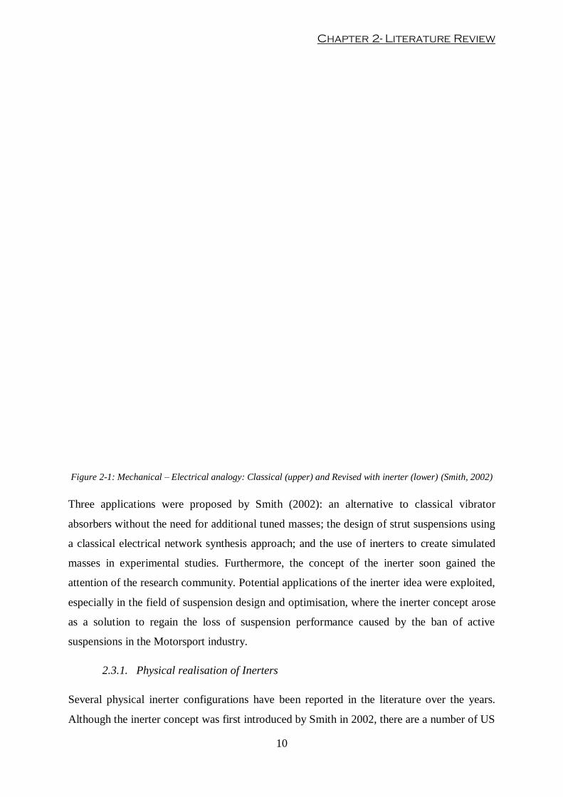
masses to grounded capacitors (upper diagram in Figure 2-1). This classical analogy was
restricted in its realization since no mechanical element could represent a true two-terminal
capacitor. However, inerters can replace masses in the analogy since these ports represent
true two- terminal capacitors (lower diagram in Figure 2-1). In this revised analogy, a mass
port could be considered as a special case of inerter in which one of the terminals is
grounded. Moreover, the most important implication of this new mechanical-electrical
analogy resides in the fact that all network synthesis and analysis techniques developed for
decades in Electrical Engineering could be theoretically applied without any restrictions.
Chapter 2- Literature Review
10
Figure 2-1: Mechanical – Electrical analogy: Classical (upper) and Revised with inerter (lower) (Smith, 2002)
Three applications were proposed by Smith (2002): an alternative to classical vibrator
absorbers without the need for additional tuned masses; the design of strut suspensions using
a classical electrical network synthesis approach; and the use of inerters to create simulated
masses in experimental studies. Furthermore, the concept of the inerter soon gained the
attention of the research community. Potential applications of the inerter idea were exploited,
especially in the field of suspension design and optimisation, where the inerter concept arose
as a solution to regain the loss of suspension performance caused by the ban of active
suspensions in the Motorsport industry.
2.3.1. Physical realisation of Inerters
Several physical inerter configurations have been reported in the literature over the years.
Although the inerter concept was first introduced by Smith in 2002, there are a number of US
Optimisation of racing car suspensions featuring inerters
11
patents that reveal the development of mechanical inerters. The design of the first physical
inerter dates back to the beginning of 20th
Century (Watres, 1908). Although, the mechanism
presented in this patent was not named as an inerter at that time, the working principle and
construction corresponds nowadays to what we now understand as an inerter. The aim of this
device was to provide a shock absorbing action in early automotive carriages. Several
modifications of this early inerter design were made in the coming years. King (1912)
developed a ballscrew mechanism coupled with an internal spring in order to provide
suspension effects between the carriage and the axle. Tauscher (1928) conceived a double-
spring ballscrew inerter mechanism to absorb shocks in a rear axle motor vehicle suspension.
A variant of this early spring-inerter mechanism was also applied to absorb vibrations in door
spring hinges (Seqveland, 1933). More complex designs were subsequently developed in
following years (Bleakney, et al., 1949; Gies & Rumsey, 1962). Those mechanisms were
intended to control the vibrations produced in aircraft wings and other truss structures.
The first design patent that refers to what we now understand as an inerter dates from 2009
(Wang, et al., 2009). Different variants of a ballscrew inerter were proposed. An alternative
to the ballscrew inerter, Smith (2002) was on a rack-and-pinion mechanism. In both designs,
the working principle is very similar: the relative translational movement between terminals
is transformed by some means (ballscrew or rack-and-pinion mechanism) into a rotational
movement in a flywheel. With the ballscrew design solution, the inertance is characterised by
inertia of the flywheel and the lead of the screw whereas, with the rack-and-pinion solution,
the inertance characteristic depends on inertia of the flywheel and gear ratio between rack and
pinion. A slightly different approach was proposed by Wang et al. (2011). In this design,
fluid inside a hydraulic system is used to generate differential pressures in a hydraulic motor
which, at the same time, induces a rotational acceleration in a flywheel. Results of
experimental testing of the hydraulic inerter show significant deviations from theoretical
ideal inerter behaviour. A more complex configuration was developed by Wang and Chan
(2008). In this work, a semi-active inerter is developed as a Permanent Magnet Electric
Motor (PMEM) is coupled with a passive mechanical ballscrew inerter. Wang suggested that
virtually any mechanical network could be synthesized with the use of mechatronic inerters.
2.3.2. Inerter Technology applied to Vehicle Suspension Dynamics
Shortly after his first publication, Smith (2003) focused his attention on the application of
inerters into vehicle suspensions as an alternative to active suspensions. The article focused
Chapter 2- Literature Review
12
on the realization of passive mechanical networks to obtain optimised suspension
configurations. Moreover, in a research paper published by Smith and Wang (2004), an
extensive theoretical investigation was carried out in order to study the potential benefits of
inerters in vehicle suspensions. Several suspension layouts incorporating inerters were
proposed and suspension parameters were optimised with respect to some prescribed
objective functions. The study was carried out for a quarter-car vehicle model and for a full
car vehicle model. In both studies, experimental data for a real inerter was briefly presented
but no actual validated vehicle models were developed.
Papageorgiou and Smith (2005) were the first to publish research work related to
experimental testing of inerters. In this work, experimental rack-and-pinion and ballscrew
inerters were designed and tested on a rig test facility. Experimental data was provided but no
real inerter model is obtained. Wang and Su (2008) presented an extension of previous
experimental work done in the field. Using the same inerter device, a validated nonlinear
inerter model was proposed. The experiments carried out in these articles, analyse the inerter
in isolation. Results showed that the model provided a good agreement between simulation
and experimental data. This nonlinear inerter model was then used to optimise a theoretical
quarter-car vehicle suspension model. The effects of inerter nonlinearities in suspension
performance were analysed. Results of this analysis showed that, according to the objective
functions defined by the authors, nonlinearities reduced the efficiency of the inerter in
suspension optimisation.
2.3.3. Inerter Technology applied to other Engineering fields
The inerter concept has been also applied to other engineering fields. Wang et al. (2006)
studied the application of inerters in train suspension systems in order to improve passenger
comfort and train stability. Evangelou et al. (2007) carried out a theoretical study for the
design of passive mechanical steering compensator for high performance motorcycles.
Investigations showed that potential improved dynamic motorcycle responses in wobble and
weave vibration modes could be obtained simultaneously with the use of inerters.
Papageorgiou et al. (2007) extended this research work and proposed the design of an
experimental passive mechanical steering compensator for motorcycle. The device was
designed as a damper in series with an inerter and tested on a purpose-built test bench. A
comprehensive nonlinear validated model was obtained from experimental testing. Inerter
technology has also been studied in Structural Engineering. Several studies analysed the

Optimisation of racing car suspensions featuring inerters
13
potential improvement of building vibration isolation performance with inerters. Wang et al.
(2007) carried out a theoretical optimisation using three different elastic foundations for
different building structures. Performance gains were obtained by the use of inerters in all
cases. Wang et al. (2010) extended previous research work. This work included an additional
building foundation layout. Experimental testing was carried out in a purpose-built test bench
but the behaviour of the real inerter was briefly discussed.
All experimental studies reported in literature are limited to the analysis of a real inerter
device in isolation. There are no reported studies in the literature that suggest an integrated
analysis of real inerters into vehicle suspensions. Several suspension models have been used
in literature in order to study the potential benefits of inerters in vehicle suspensions.
However, none of these models have been validated against suspension experimental data
coming from four or seven post rig facilities.
2.4. Experimental Testing on Vehicle Suspensions
Experimental testing provides a method of tuning and analysing different suspension options
according to specific objectives. The main ways a vehicle suspension can be tested are: track
testing and laboratory rig testing.
Laboratory testing offers a much more cost-effective and controlled environment than
physical testing on the track. The main aim of a suspension test rig is twofold: on one hand,
rigs are used to apply fundamental inputs in order to characterise and estimate parameters;
and, on the other hand, they use controlled actuators to recreate external dynamic actions
applied to the vehicle suspension. Suspension test rigs can be classified according to the
number of actuators used: quarter-car test rigs, four-post test rigs and seven-post test rigs are
the most common ones, although eight-post test rigs have also been developed (Southward &
Boggs, 2008).
Quarter-car test rigs are designed to study the fundamental dynamics of a suspension without
the need of having a full vehicle or prototype present on the test. In these rigs, the sprung
mass is limited to move only vertically relative to the reference frame, while the suspension
and tyre coupling can be designed in different ways depending on the nature of the study
carried out. Figure 2-2 shows an example of the quarter-car test rig used in Virginia
Polytechnic Institute (Andersen, 2007).
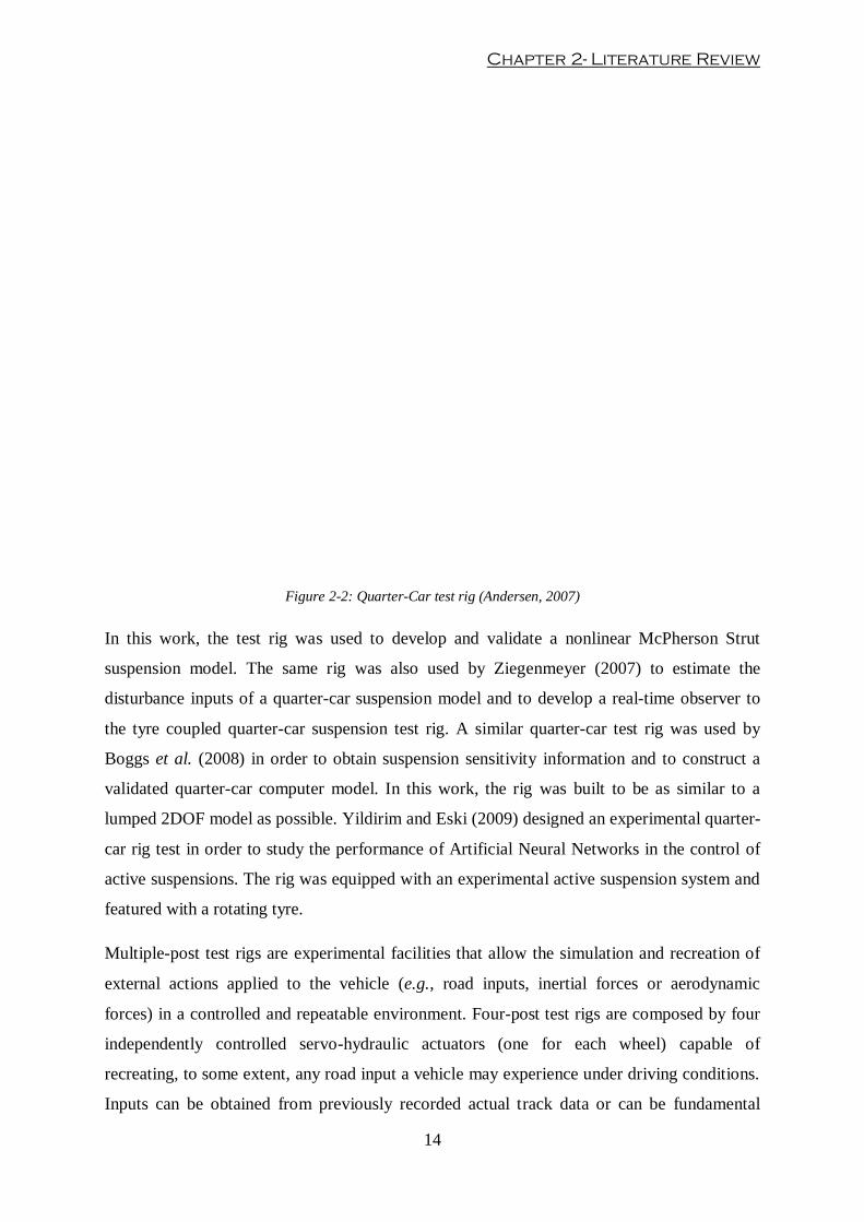
Chapter 2- Literature Review
14
Figure 2-2: Quarter-Car test rig (Andersen, 2007)
In this work, the test rig was used to develop and validate a nonlinear McPherson Strut
suspension model. The same rig was also used by Ziegenmeyer (2007) to estimate the
disturbance inputs of a quarter-car suspension model and to develop a real-time observer to
the tyre coupled quarter-car suspension test rig. A similar quarter-car test rig was used by
Boggs et al. (2008) in order to obtain suspension sensitivity information and to construct a
validated quarter-car computer model. In this work, the rig was built to be as similar to a
lumped 2DOF model as possible. Yildirim and Eski (2009) designed an experimental quarter-
car rig test in order to study the performance of Artificial Neural Networks in the control of
active suspensions. The rig was equipped with an experimental active suspension system and
featured with a rotating tyre.
Multiple-post test rigs are experimental facilities that allow the simulation and recreation of
external actions applied to the vehicle (e.g., road inputs, inertial forces or aerodynamic
forces) in a controlled and repeatable environment. Four-post test rigs are composed by four
independently controlled servo-hydraulic actuators (one for each wheel) capable of
recreating, to some extent, any road input a vehicle may experience under driving conditions.
Inputs can be obtained from previously recorded actual track data or can be fundamental

Optimisation of racing car suspensions featuring inerters
15
mathematical functions (e.g. sine waves or step inputs). Measurement systems are fitted to
the test vehicle so that dynamic characteristics of the vehicle, suspensions and tyres can be
determined and suspension setup changes can be assessed and optimized (Kowalczyk, 2002;
Cambiaghi, et al., 1998; Maher, 2011). Four-post rigs are often provided with additional non-
controlled (one or two) pneumatic actuators. These actuators can only provide static forces
that are normally used to set vehicle suspension within the normal operating range. As
opposed to four-post rigs, seven-post rig facilities incorporate three additional controllable
actuators connected to the chassis (conventionally referred to them as ‘aeroloaders’) that
allow the combined analysis of road excitation with aerodynamic and inertial effects (Kelly,
et al., 2002). Eight-post rigs are composed by four road excitation actuators and four
‘aeroloaders’. These rigs offer the added capability of analysing the dynamic warp stiffness
of the vehicle more accurately than seven-post rigs (Southward & Boggs, 2008). In general,
more actuators offer added value to the tests performed. However, multi–post test rigs are
multiple input/multiple output (MIMO) systems which require high levels of control (Fricke
& Hogg, 2010). Hence, more actuators require the development of more complex control
algorithms.
Examples of racing car suspension characterisation and optimisation in test rig facilities are
very sparse in literature. Boggs et al. (2009) used experimental data from 7-post rig testing to
produce an efficient vehicle parameter identification method. Miller (2002) tested a Formula
SAE car on a 7-post rig in order to optimise anti-roll bar and damper settings. A case study of
ChampCar damper optimisation was presented by Kowalczyk (2002). Results show that,
when using multiple criteria for optimising a suspension, trade-off among objectives
functions is obtained. However, no reported studies in literature investigate the use of a 4-
post rig test facility to analyse vehicle suspensions incorporating real inerters.
2.5. Virtual Suspension Simulation
Vehicle suspension models are commonly used in dynamic analysis. They are powerful tools
for virtual suspension design and optimisation. These models allow the analysis of the impact
of different suspension settings on the performance of the vehicle in a cost and time efficient
way (Soliman, et al., 2001; Rakheja & Ahmed, 1991; Barak, et al., 2004; Soliman, et al.,
2008). Vehicle suspension models can also be used in optimisation in order to determine
optimal suspension configurations with respect to some prescribed objective functions
Chapter 2- Literature Review
16
(Metwalli, 1986; Alkhatib, et al., 2004; Georgiou, et al., 2007; Verros, et al., 2005; Kuo, et
al., 2008).
While simple suspension models are useful for gaining a general understanding of the system,
more comprehensive models are required for accurate description of suspension dynamic
behaviour and for efficient suspension optimisation. The complexity of these models depends
on the number of DOF considered and the design of the particular suspension components
(e.g. passive, semi-active or fully active suspensions, design of nonlinearities or modelling of
parasitic effects). The following sections review the most relevant vehicle suspension models
that can be found in reported literature.
2.5.1. Modelling of vehicle equations of motion
The simplest suspension model is a single degree-of-freedom (SDOF) system. This simplistic
system assumes that the vehicle can be modelled as a point mass that moves along the
vertical axis and that the tyres can be modelled as an equivalent massless linear spring. The
use of this type of model is very rare in suspension analysis due to its crude representation of
the behaviour of the physical vehicle. Storey et al. (2006) used a SDOF model to investigate
the performance of different active and semi-active suspension systems. Alkhatib et al.
(2004) used a linear SDOF to obtain optimal spring and damper rates with the aid of a
Genetic Algorithm (GA). A more complex model includes the effect of unsprung mass in the
dynamic response of the vehicle. This is the so-called quarter-car vehicle model or 2-DOF
vehicle model. The use of quarter-car models has been widely reported in literature due to its
simplicity and yet its relative accuracy in simulating the main vibration modes of the vehicle
(body and hub vibration modes). Several authors used quarter-car models in order to carry
out suspension analysis (Rakheja & Ahmed, 1991; Soliman, et al., 2001; Jazar, et al., 2006),
and suspension optimisation (Metwalli, 1986; Alkhatib, et al., 2004; Georgiou, et al., 2007;
Verros, et al., 2005; Gobbi, et al., 2006; Chi, et al., 2008). The next step in vehicle suspension
modelling complexity is the so-called half-car model. Half-car models are common in
literature. These models assume that the main body (sprung mass) presents two predominant
motions: a translational (vertical) motion as well as a rotation around either roll or pitch axis.
Sun et al. (2002) used a 4-DOF system to represent a half-car vehicle model. In this work, the
model was used to analyse the effect of suspension parameters on the transient response of
the vehicle. Soliman et al. (2008) used half-car models in roll and pitch planes in order to
analyse the impact of the main suspension parameters in the dynamic response of the vehicle.

Optimisation of racing car suspensions featuring inerters
17
Extended half-car models that consider aerodynamic effects have been developed in order to
analyse the interaction between aerodynamics and ride dynamics (Floyd & Law, 1994;
Abdelhady, 2002). Kuo et al. (2008) and Sun and Chen (2003) used a half-car 4-DOF model
in order to perform suspension optimisation. An improvement of the previous model is the
extension to 7DOF suspension models. These models allow the simulation of the vertical ride
dynamics of a full car as well as all the rotational modes simultaneously (pitch, roll and
warp). Barak et al. (2004) developed a full-car vehicle model in order to analyse the dynamic
behaviour of a full suspension. Abdelhady and Crolla (1989) used a 7-DOF vehicle model in
order to investigate the theoretical performance benefits of active suspensions with respect to
passive systems. In Wang et al. (2006), Shannan and Vanderploeg (1989) and Lu and
DePoyster (2002), full-car vehicle models were also developed to study the performance of
active suspensions in combined ride and handling manoeuvres. More complex models are
less frequent in suspension modelling literature. These complex models often incorporate
additional degrees of freedom in order to improve accuracy and reliability. Shirahatt et al.
(2008) and Del Castillo et al. (1990) produced vehicle models with an additional DOF for the
vertical movement of a driver. Graf and Kosuch (2008) introduced an extended full-car
model. This model presented an additional DOF which accounts for compliance in the
chassis. The chassis was modelled as two rigid bodies connected by a torsional spring.
2.5.2. Modelling of individual suspension components
Suspension model complexity also depends on the details with which suspension features are
modelled. Many studies in literature model a suspension as a linear combination of a spring
in parallel with a damper (and an additional force in the case of active suspensions)
regardless of whether these components present linear or nonlinear characteristics.
(Deshpande, et al., 2006) modelled a secondary suspension system coupled to the main
suspension system to investigate the effect of jump avoidance. In (Stamatov, et al., 2007),
parasitic effects were modelled as part of the suspension strut. Elastic compliance due to
bushings and damper friction effects are also included in this model. Other models include
suspension kinematics in the dynamic model (Balike, 2010; Andersen, 2007; Al-Holou, et al.,
2002). In the past few years, different vehicle suspension models featuring inerters have also
been proposed in order to evaluate the potential benefits of inerters in suspension
optimisation (Smith & Wang, 2004; Scheibe & Smith, 2009). However, these vehicle
suspension models were proposed from a theoretical point of view but they were never
validated against experimental data. No reported works that validate vehicle suspension

Chapter 2- Literature Review
18
models incorporating inerters against experimental suspension data have been found in
literature.
In addition to suspension components, tyres must also be modeled. Captain et al. (1979)
presented four different vertical tyre models. In this study, guidelines for the selection of the
most suitable tyre model were provided. However, over the years, most of vertical suspension
models reported in literature consider a linear single contact point tyre model. In its most
basic configuration, this tyre can be modeled as a linear spring that represents the flexibility
characteristic of a tyre (Williams & Haddad, 1997; Williams, 1997; Sharp, et al., 1987). This
model can be extended in order to account for tyre energy dissipation effects. This term is
commonly modeled as a damping effect (Akcay & Turkay, 2009; Graf & Kosuch, 2008).
Although this tyre model is widespread in the field of Suspension Dynamics due to its
simplicity, no reported literature has been found that correlates this model against
experimental data. A more complex nonlinear semi-empirical vertical tyre model was
developed by Pacjeka (2006). Experimental data obtained from tyre rig testing was used to
create this semi-empirical model. However, the main drawback of this model is that it
requires the tyre to be tested experimentally to be able to integrate the model into simulation.
No reported studies that use this vertical tyre model for suspension simulation have been
found.
2.6. Suspension Optimisation
Suspension optimisation has been a topic of growing interest for research in the last decades.
The development of suspension models allows the use of different optimisation algorithms to
search through the design space for an optimal suspension setting according to some
predefined objective functions in a robust and efficient way (Gobbi, et al., 1999; Chi, et al.,
2008; Shirahatt, et al., 2008; Verros, et al., 2005). In current motor racing, where cost
reduction is of paramount concern, computer algorithms can be quite useful for efficient
suspension design and optimisation. The use of virtual optimisation tools reduces the time of
track testing and provides a better understanding of the vehicle suspension. The ult imate goal
of this optimisation process is to obtain a suspension setting that optimises the overall
performance of the car. In mathematical terms, a general minimisation problem can be
expressed as follows (Antoniou & Lu, 2007):
Optimisation of racing car suspensions featuring inerters
19
Where S represents a set of tunable parameters (or “search space”) and f represents the
function to be minimised (or “cost function”).
According to this definition, the success in achieving this goal depends largely on two key
factors:
Selection of objective functions f.
Development of a robust and efficient optimisation methodology.
A review of the literature is provided in the following sections with regard to the selection of
objective function for suspension optimisation and the development of a suspension
optimisation method.
2.6.1. Performance Objective Functions for Suspension Systems
The selection of these objective functions is a paramount concern in suspension design and
optimisation. As expressed in eq. (2.2), the outcome of an optimisation problem is a set of
parameters S that minimises the value of an objective function f. Hence, objective functions
must be chosen so that they accurately represent the goals a suspension designer is trying to
achieve. Furthermore, the performance of an optimisation algorithm depends largely on the
configuration of the cost function, i.e. cost functions must be created in such a way that the
optimiser can efficiently extract useful information from them to continue with the search.
Most of the work found in literature is related to the definition of objective indexes for
production car suspension optimisation (Sharp, et al., 1987; Georgiou, et al., 2007; Gobbi, et
al., 2006; Li & Kuo, 2000).
In suspension analysis, vehicle comfort is commonly defined as the amount of vertical
acceleration transmitted from road to the sprung mass and ultimately, to the driver and
passengers. The most common mathematical function selected to express comfort is root-
mean-square (RMS) due to the intrinsic continuity and differentiability of this mathematical
function. (Jazar, et al., 2006; Hegazy & Sandy, 2009; Sun & Chen, 2003; Gobbi, et al., 2006;
Georgiou, et al., 2007; Sun, et al., 2010; Thompson, 1973). A more complex comfort index
was introduced by Johnson et al. (2010). In this research work, different objective functions
were presented and their performance was discussed.
Vehicle safety is defined as tyre/road holding. It is well reported that the fluctuations in
vertical loads applied to the tyres influence strongly their ability to produce longitudinal and

Chapter 2- Literature Review
20
lateral forces (Gillespie, 1992; Milliken & Milliken, 1995; Pacjeka, 2006). Thus, reduction of
tyre load fluctuations can then provide a more robust and closely controlled vehicle response.
As with ride comfort index, the function chosen in literature to express vehicle safety (or
control) is the RMS of the dynamic tyre load fluctuation (Verros, et al., 2005; Georgiou, et
al., 2007; Cooke, et al., 1997; Thompson, 1983).
Rattle space or suspension working space has also been considered as an objective function in
road car suspension optimisation. Suspension travel defines vehicle suspension packaging,
suspension kinematics characteristics and suspended body minimum ride heights, so
controlling its magnitude is important for suspension design. An RMS of suspension stroke is
used as well (Verros, et al., 2005; Molina-Cristobal, et al., 2007; Georgiou & Natsiavas,
2009).
All these suspension objectives focus on the ride performance of the vehicle, and little
attention is paid to the effects of suspension on the handling characteristics of the vehicle.
Moreover, given the competitive nature of motorsport industry, objective functions related to
vehicle performance rarely enter the public domain. It was demonstrated that the control of
suspension parameters have an important effect on handling characteristics (Wang, et al.,
2006; Cooke, et al., 1997; Shim & Margolis, 2005; Blank & Margolis, 1996; Miura, et al.,
2004). Only a few studies are found to measure handling as well as ride functions (Gobbi, et
al., 1999; Benedetti, et al., 2006). However, in these studies, the handling functions were
limited to prescribed manoeuvres, and the direct relationship between suspension parameters
and the impact of suspension dynamics on overall vehicle performance was not discussed.
Moreover, these suspension cost functions have been mostly developed from quarter-car
studies, where only vertical motion is considered. Very little literature can be found on the
definition of objective functions accounting for rotational vibration modes as well as
translational (vertical) modes. Most of these studies proposed a sum of the weighted terms
where weighting terms were selected arbitrarily (Hrovat, 1997). Furthermore, these indices
have been mainly applied to studies for production road cars that operate well inside the
limits of adhesion. However, in motor racing, race cars are constantly operating at the limits
of tyre adhesion. In this situation, handling characteristics are highly coupled with ride
performance of the suspension (Mashadi & Crolla, 2005). In this study, it was demonstrated
that the understeer characteristics of a vehicle at relatively high lateral accelerations (~ 1g)
can vary sharply due to the effect of suspension dynamics. However, this study did not
propose objective functions to deal with this behaviour. Blank and Margolis (1996) proposed

Optimisation of racing car suspensions featuring inerters
21
functions that related lateral and vertical dynamics for a quarter-car model but no relationship
to overall vehicle performance was discussed. In current Formula 1 (F1) cars, aerodynamics
is a key factor in the overall performance of the vehicle. There are studies in literature that
highlighted the coupling between aerodynamics and suspension dynamics (Floyd & Law,
1994; Aschwanden, et al., 2006; Aschwanden, et al., 2008). However, none of these studies
developed objectives functions for suspension optimisation accounting for aerodynamic
performance. Moreover, there are no reported studies in literature that investigate the effect
of coupled ride and handling dynamics on the overall performance of a race car through lap-
time simulation (LTS) or physical track testing.
2.6.2. Multi-objective Optimisation Algorithm
Suspension systems are a critical part of a racing vehicle because they are the only physical
linkage between tyres and chassis. Moreover, from a purely dynamic point of view, the main
goals of a vehicle suspension are (Gillespie, 1992):
To keep the tyres in contact with race track.
To resist chassis motions induced by external forces (inertial and aerodynamic
forces).
To control the weight balance across all four tyres under dynamic situations.
In order to achieve these goals and therefore maximise vehicle performance, suspension
design must be translated into an optimisation problem (see equation (2.2)). A vast variety of
general mathematical optimisation algorithms is available in literature (Venkatamaran, 2002;
Antoniou & Lu, 2007; Weise, 2011). In this section, only the most relevant algorithms
applied to suspension design and optimisation have been reviewed.
Many reported studies dealing with suspension optimisation can be found in literature.
Thoresson et al. (2009) and (2009b) successfully applied a Dynamic-Q gradient-based
algorithm to single-objective suspension optimisation problem. Els et al. (2006) compared
the performance of two gradient-based single-objective optimisation methods: a Sequential
Quadratic Programming (SQP) and a Dynamic-Q method. The study suggested that the SQP
method was more efficient and robust. Chi et al. (2008) ran a comparative study of three
optimisation algorithms: Evolutionary Algorithm (EA), Pattern Search Algorithm (PSA) and
Sequential Quadratic Program (SQP). Results showed that gradient-based algorithms
provided strong and efficient local convergence. The number of function evaluations was
Chapter 2- Literature Review
22
lower, therefore making them very computationally efficient. However, these methods
required gradient and Hessian information of the objective function, which could be either
provided by the user or sorted by the software itself using finite differences approximation
method, meaning that this approach would be poor when dealing with systems with
discontinuities, nonlinearities or discrete functions. Furthermore, gradient-based approaches
do not guarantee to find the global optimum of the problem. Alternatively, non gradient-
based algorithms such as EAs and PSA use meta-heuristic methods for searching optimal
solutions through the design space. Optimal solutions are evolved from generation to
generation in a stochastic, discrete and nonlinear process (Man, et al., 1996). No gradient
information is required so they are more powerful in finding a near global optimum.
However, EAs present some disadvantages with respect to local gradient-based search
techniques: due to the population based search approach of EAs, the optimisation process is
computationally expensive and simulation times are often high. Another drawback is that the
efficiency and the reliability of the algorithm depend largely on the parameters used to set the
optimisation problem (e.g. population size, crossover probability, mutation probability,
percentage of elistist individuals). Baumal et al. (1998) used a single-objective Genetic
Algorithm (GA) in order to optimise ride comfort with an active suspension. Li and Kuo
(2000) successfully applied an EA to single-objective passive suspension optimisation. A
different optimisation approach was proposed by Sun and Chen (2003) and Papageorgiou and
Smith (2006). In this approach, linear matrix inequalities (LMIs) were used to synthesise
optimised suspension layouts.
All previous studies considered the optimisation of a single suspension objective function.
However, as mentioned at the beginning of the section, optimal suspension design requires
the optimisation of several objective functions simultaneously. Therefore, the suspension
optimisation problem must be considered as a general multi-objective optimisation problem
(MOOP). A general MOOP can be mathematically expressed as follows (Deb, 2001):

Optimisation of racing car suspensions featuring inerters
23
Where x={x1, x2, ... , xn} is the vector of n decision variables
F(x) is the vector of m objective functions
G(x) is the vector of j inequality constraints
H(x) is the vector of k equality constraints
xiL, xiU are the limits of the search space for the i-th decision variable
Traditional gradient-based optimisation techniques present an important limitation: the
MOOP must be re-formulated into a single-objective optimisation problem so that objective
function gradient information can be acquired. This means that interactions between objective
functions cannot be studied independently. Alternatively, the meta-heuristic nature and the
population-based approach of EAs make them well-suited to solve real MOOPs (Deb, 2001;
Sbalzarini, et al., 2000). However, due to the diversity of the MOOPs, it is rarely possible to
use the standard EA, instead, over the years, several variants and modifications have been
developed to try to cope with the singularities of each problem. Several EA comparative
studies can be found in literature (Zitzler, et al., 2000; Konak, et al., 2006; Fonseca &
Fleming, 1995). These studies analyse the performance and robustness of different EAs under
different test problems. Results from these studies show that elitist EAs offer enhanced
performance capabilities with respect to non-elitist EAs. In particular, the elitist non-
dominated sorting genetic algorithm (NSGA-II) outperforms other contemporary EAs in
terms of convergence to near-true Pareto-optimal sets (Deb, et al., 2002). Moreover, EAs can
be coupled with local gradient-based search algorithms to improve the efficiency of the
optimisation algorithm and to ensure that the true Pareto optimal set is obtained (Deb & Goel,
2001). Several approaches using multi-objective EAs have been applied to suspension
design. Cheli et al. (2007) applied a multi-objective EA to optimise the kinematic
characteristics of an active suspension. Loyer and Jézéquel (2009) used an EA to obtain a
Pareto optimal set of a passive quarter car linear suspension. Molina-Cristobal et al. (2007)
applied a multi-objective EA to obtain an optimised ideal suspension mechanical network
featuring inerters.
2.6.3. Surrogate Model Based Optimisation
EAs are well-suited for solving true multi-objective optimisation problems due to their
population-based searching approach. However, in order to find the true Pareto optimal set,
Chapter 2- Literature Review
24
the computational effort require is high. Real-life engineering problems usually involve
simulation of high-fidelity and complex virtual models, where large search spaces and
multiple objective functions need to be optimised. Moreover, in these optimisation problems,
every time the objective function is evaluated, the solution of the dynamic system must be
computed via numerical integration techniques. This means that the sole use of EAs can
become computationally very intensive. Alternatively, metamodelling techniques can be used
in combination with an EA in order to enhance the computational efficiency of the
optimisation method (Bramanti, et al., 2001). Surrogate models, or metamodels, are compact
analytic models that approximate the dynamic behaviour of complex systems. Surrogate
models are constructed through data obtained from a limited set of simulations of the original
model (Forrester, et al., 2008). The input/output nature of surrogate provides direct and fast
relationships between performance objectives and design variables (Queipo, et al., 2005).
Surrogate model based optimisation has been successfully applied to different engineering
fields: Bouazizi et al. (2009), applied this approach to structural design; Chung and Alonso
(2004) used a surrogate model in combination with a hybrid EA to design the external profile
of a low-boom supersonic business jet; Vaidyanathan et al. (2004) and Goel et al. (2007)
created an approximate model of a model of a single-element rocket injector in order to
efficiently optimise the performance of the injector; Lyu et al. (2006) used the surrogate-
based approach to optimise the torsion beam in a vehicle suspension system; and Cappelleri
et al. (2002) applied a metamodel-based approach to design a piezoelectric bimorph actuator.
Examples of metamodelling studies can also be found in the field of Vehicle Dynamics. Butz
et al. (2010) created a metamodel of a vehicle multi-body dynamic system in order to
estimate suspension parameters. Chen et al. (1999) used a surrogate model based approach to
improve the handling characteristics of a vehicle. Gobbi et al. (1999) and Benedetti et al.
(2006) used a metamodel based optimisation method in order to determine a suspension
setting for optimal handling characteristics. Yang and Huang (2009) and Wentao et al. (2011)
used the same approach to improve ride comfort and safety of a road car.
A formal process of surrogate model based multi-objective optimisation was established by
Wilson et al. (2001) and it can be summarised in the following diagram:
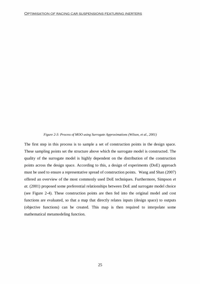
Optimisation of racing car suspensions featuring inerters
25
Figure 2-3: Process of MOO using Surrogate Approximations (Wilson, et al., 2001)
The first step in this process is to sample a set of construction points in the design space.
These sampling points set the structure above which the surrogate model is constructed. The
quality of the surrogate model is highly dependent on the distribution of the construction
points across the design space. According to this, a design of experiments (DoE) approach
must be used to ensure a representative spread of construction points. Wang and Shan (2007)
offered an overview of the most commonly used DoE techniques. Furthermore, Simpson et
at. (2001) proposed some preferential relationships between DoE and surrogate model choice
(see Figure 2-4). These construction points are then fed into the original model and cost
functions are evaluated, so that a map that directly relates inputs (design space) to outputs
(objective functions) can be created. This map is then required to interpolate some
mathematical metamodeling function.

Chapter 2- Literature Review
26
Figure 2-4: Techniques for Metamodelling (Simpson, et al., 2001)
Several surrogate modelling techniques have been reported in literature: polynomial
regression (PR), Kriging modelling (KRG) and Radial Basis functions (RBF) are the most
widely used methods (Jin, 2005). Several studies were carried out in order to investigate the
performance of each metamodelling technique (Simpson, 1998; Simpson, et al., 2001; Jin, et
al., 2000; Fang, et al., 2005; Shihani, et al., 2006). Metamodelling techniques were evaluated
in order to test different capabilities such as model creation simplicity, model response
accuracy and computational effort (measured as simulation time). These studies suggested
that a Kriging metamodelling technique offers a good compromise among all the features
tested. Kriging methods have their origins in mining and geostatistical applications. This
method is a combined model that can be defined as follows:
Where f(x) represents a global approximation of the original function and it is expressed as a
polynomial model and Z(x) is expressed as a stochastic function that represents localised
deviations in between data samples (Simpson, et al., 2001).
The following step is to validate the predictive capabilities of the approximate model. A new
set of random sampling points is generated and used to evaluate the quality of the
Optimisation of racing car suspensions featuring inerters
27
approximate model with respect to the original model. The most common statistical metrics
used to evaluate the accuracy and predictability of the surrogate model are the root mean
square error (RMSE) and maximum absolute error (MAE) (Wang & Shan, 2007).
Alternatively, more exhaustive comparative studies present more complex statistical metrics
such as R2, relative average absolute error (RAAE), or relative maximum absolute error
(RMAE) (Jin, et al., 2000). Once the metamodel has been validated, it can be used in
substitution of the original computationally expensive model as the input of the optimisation
process.
2.7. Lap-Time Simulation
The use of lap-time simulation (LTS) tools is important in the design and development of
race cars. LTS packages simulate a vehicle model negotiating a race track. LTS tools can
provide significant advantages to race teams since different designs and settings can be
virtually tested without the need of building a prototype and of track testing. Thus, a LTS
package is more cost and time effective than physical track testing and allows modifications
on fundamental parameters of the vehicle design.
LTS packages simulate a vehicle completing a lap on race track in the minimum time
possible. In order to do so, equations of motion (EOMs) of the vehicle system must be solved
to find the on-limit adhesion conditions. According to this, LTS tools can be classified into
three categories depending on the strategy used to solve these EOMs (Siegler, et al., 2000):
Static or Steady-State Strategy.
Quasi-static or Quasi-Steady-State Strategy (QSS).
Transient Strategy.
In a Steady-State strategy, the race track is divided into straights and constant radius corners.
Longitudinal and lateral motions are completely decoupled and all the time-dependent terms
are neglected. Only lateral acceleration due to circular motion is accounted for in this
strategy. This strategy is barely used for accurate LTS studies due to its simplicity.
A QSS strategy represents an extension of the previous strategy. In this approach corners are
divided into a set of constant radius turns. Each of these segments will be of different corner
radius, i.e. decreasing corner radius up to corner apex and increasing from it.

Chapter 2- Literature Review
28
At each segment, a balance in the forces applied to the vehicle exists. The vehicle is assumed
to be moving from one state to the immediate next state in a steady fashion. Lateral
acceleration is obtained from equations derived for a constant radius motion and a tyre model
is then used to obtain the lateral force needed to maintain this lateral acceleration. The
longitudinal tyre forces used to accelerate the vehicle longitudinally can then be calculated
from either a combined tyre model such as Pacejka Magic Formula (Pacjeka, 2006) or from a
tyre friction circle approach (Milliken & Milliken, 1995). The accuracy of this strategy
depends on the length of the corner segment used in simulation. Examples of this QSS
strategy can be found in (Brayshaw, 2004; Braghin, et al., 2008).
The most important limitation found in the previous two strategies is that no transient effects
are accounted for in the simulation. The third strategy is used to overcome this limitation. In a
transient strategy, the fully transient solution of the dynamic system is obtained. Since the
objective of the present research work is to study and optimise the dynamics of a race car
suspension, attention is focused on the discussion of transient LTS in the following sections.
2.7.1. Previous work on Transient Lap-Time Simulation
Transient LTSs carry out the non-steady simulation of a vehicle around a race track. In this
strategy, numerical integration of fully dynamic EOMs of the vehicle for each instant of time
is carried out. Due to the competitive nature of Motorsport, only a few studies with regard to
the design and development of transient LTS have been reported in literature. The first
attempt at developing a transient optimal LTS dates from late 1980s. Metz and Williams
(1989) used a simple 3-DOF planar vehicle model to estimate the minimum time in a
prescribed short distance manoeuvre. Fujioka and Kimura (1992) proposed a similar method
in order to carry out an analysis of steering and powertrain systems. A different solution
method was proposed by Hendrikx et al. (1996): the lap-time simulation time problem was
solved in the distance domain rather than in the time domain. In these works, transient LTS
was solved as a minimum time manoeuvring (MTM) problem. Optimal control inputs were
then obtained to solve the MTM problem via OC solution methods (see section 2.7.2).
The first complete lap transient LTS was developed by Casanova (2000). Casanova
developed a method for solving the MTM problem based on Optimal Control (OC) theory. In
his work, the LTS problem was proposed as a time Optimal Control problem. The OC was
then transcribed to a Non-linear Programming (NLP) problem via a parallel shooting direct
method. Casanova identified two limitations in this procedure: computational effort to solve
Optimisation of racing car suspensions featuring inerters
29
the OC problem and sensitivity of objectives and constraints stability with respect to early
controls. Automatic differentiation (AD) was proposed in his research work as a method to
increase the computation efficiency. In order to reduce the sensitivity to early control inputs,
the race track was split into shorter sections where optimal control problem was solved
independently and then re-attached to the global solution. Several studies resulted from this
work: a study of the significance of yaw inertia in the performance of the car (Casanova, et
al., 2000), a sensitivity study of the significance of vehicle mass (Casanova, et al., 2001), and
a study of the impact in lap time of longitudinal CoG location (Casanova, et al., 2002) were
successfully carried out by using this LTS. Kelly (2008) developed an alternative OC
algorithm for obtaining the optimal lap time based on Receding Horizon Control/ Model
Predictive Control (RHC/MPC) theory. This work was based on a previous publication by
Velenis and Tsiotras (2005). The use of MPC algorithms solved the dependency of final
convergence to initial control input guesses. However, this algorithm was computationally
very expensive.
In both methods proposed by Casanova and Kelly, driver control inputs were modelled as
open-loop controls. Current investigations propose a close-loop driver model coupled with
MPC to find the optimal racing line at constant forward speed (Timings & Cole, 2010;
Timings & Cole, 2011). Although these studies are in an experimental stage, they suggest
that both limitations could be reduced by the use of close-loop input controls.
2.7.2. Lap Time Simulation as an Optimal Control Problem
The problem of finding the minimum time manoeuvring (MTM) can be expressed as a time
Optimal Control (OC) problem (Casanova, 2000). In general terms, the OC problem can be
defined as to find a control u* that minimises a performance index J (Kirk, 2004). This can be
expressed mathematically as:
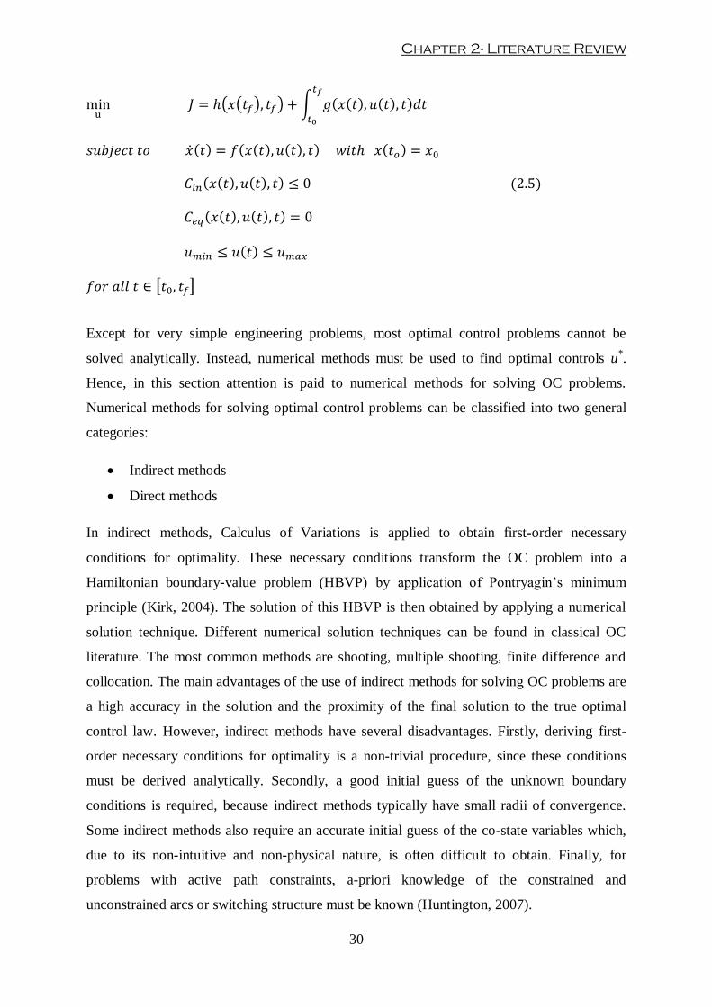
Chapter 2- Literature Review
30
Except for very simple engineering problems, most optimal control problems cannot be
solved analytically. Instead, numerical methods must be used to find optimal controls u*.
Hence, in this section attention is paid to numerical methods for solving OC problems.
Numerical methods for solving optimal control problems can be classified into two general
categories:
Indirect methods
Direct methods
In indirect methods, Calculus of Variations is applied to obtain first-order necessary
conditions for optimality. These necessary conditions transform the OC problem into a
Hamiltonian boundary-value problem (HBVP) by application of Pontryagin’s minimum
principle (Kirk, 2004). The solution of this HBVP is then obtained by applying a numerical
solution technique. Different numerical solution techniques can be found in classical OC
literature. The most common methods are shooting, multiple shooting, finite difference and
collocation. The main advantages of the use of indirect methods for solving OC problems are
a high accuracy in the solution and the proximity of the final solution to the true optimal
control law. However, indirect methods have several disadvantages. Firstly, deriving first-
order necessary conditions for optimality is a non-trivial procedure, since these conditions
must be derived analytically. Secondly, a good initial guess of the unknown boundary
conditions is required, because indirect methods typically have small radii of convergence.
Some indirect methods also require an accurate initial guess of the co-state variables which,
due to its non-intuitive and non-physical nature, is often difficult to obtain. Finally, for
problems with active path constraints, a-priori knowledge of the constrained and
unconstrained arcs or switching structure must be known (Huntington, 2007).
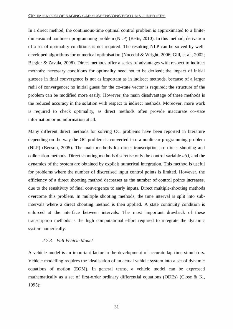
Optimisation of racing car suspensions featuring inerters
31
In a direct method, the continuous-time optimal control problem is approximated to a finite-
dimensional nonlinear programming problem (NLP) (Betts, 2010). In this method, derivation
of a set of optimality conditions is not required. The resulting NLP can be solved by well-
developed algorithms for numerical optimisation (Nocedal & Wright, 2006; Gill, et al., 2002;
Biegler & Zavala, 2008). Direct methods offer a series of advantages with respect to indirect
methods: necessary conditions for optimality need not to be derived; the impact of initial
guesses in final convergence is not as important as in indirect methods, because of a larger
radii of convergence; no initial guess for the co-state vector is required; the structure of the
problem can be modified more easily. However, the main disadvantage of these methods is
the reduced accuracy in the solution with respect to indirect methods. Moreover, more work
is required to check optimality, as direct methods often provide inaccurate co-state
information or no information at all.
Many different direct methods for solving OC problems have been reported in literature
depending on the way the OC problem is converted into a nonlinear programming problem
(NLP) (Benson, 2005). The main methods for direct transcription are direct shooting and
collocation methods. Direct shooting methods discretise only the control variable u(t), and the
dynamics of the system are obtained by explicit numerical integration. This method is useful
for problems where the number of discretised input control points is limited. However, the
efficiency of a direct shooting method decreases as the number of control points increases,
due to the sensitivity of final convergence to early inputs. Direct multiple-shooting methods
overcome this problem. In multiple shooting methods, the time interval is split into sub-
intervals where a direct shooting method is then applied. A state continuity condition is
enforced at the interface between intervals. The most important drawback of these
transcription methods is the high computational effort required to integrate the dynamic
system numerically.
2.7.3. Full Vehicle Model
A vehicle model is an important factor in the development of accurate lap time simulators.
Vehicle modelling requires the idealisation of an actual vehicle system into a set of dynamic
equations of motion (EOM). In general terms, a vehicle model can be expressed
mathematically as a set of first-order ordinary differential equations (ODEs) (Close & K.,
1995):

Chapter 2- Literature Review
32
Where x(t) represents a vector of the state variables of the system, u(t) represents the vector
of external inputs, t represents time and f is a vector value function that computes the
derivatives of the state variable vector.
The selection of an appropriate vehicle model is a compromise between model complexity,
accuracy and efficiency (Allen & Rosenthal, 1994). A more complex model will offer more
accurate results. However, a more comprehensive model will require a larger number of
ODEs to be solved per evaluation, leading to a more computationally expensive model.
Furthermore, the number of parameters required to simulate a vehicle model increases with
model sophistication.
Several vehicle models have been reported in literature. The simplest full vehicle model can
be represented as a mass point where lateral and longitudinal forces are assumed to be
directly controllable (Velenis & Tsiotras, 2005; MÜhlmeier & Müller, 2002). However, this
model does not account for fundamental vehicle under/oversteering characteristics. A better
suited model is the so-called ‘bicycle model’ (see Figure 2-5).
This is a planar vehicle model and consists of 3 DOFs: longitudinal and lateral displacement
and rotation around CoG. This model is useful to analyse the general handling characteristics
in a conceptual design stage where very little vehicle parameters are available (Milliken &
Milliken, 1995). Several examples of the use of a bicycle model have been reported in
literature (Hendrikx, et al., 1996; Velenis & Tsiotras, 2005; Schmitt, et al., 2008; Fujioka &
Kimura, 1992; Metz & Williams, 1989). In these models, longitudinal forces applied to the
tyres are assumed to be controllable inputs. An evolution of the previous model is a vehicle
model that includes tyre spin as additional DOFs (Prokop, 2001).
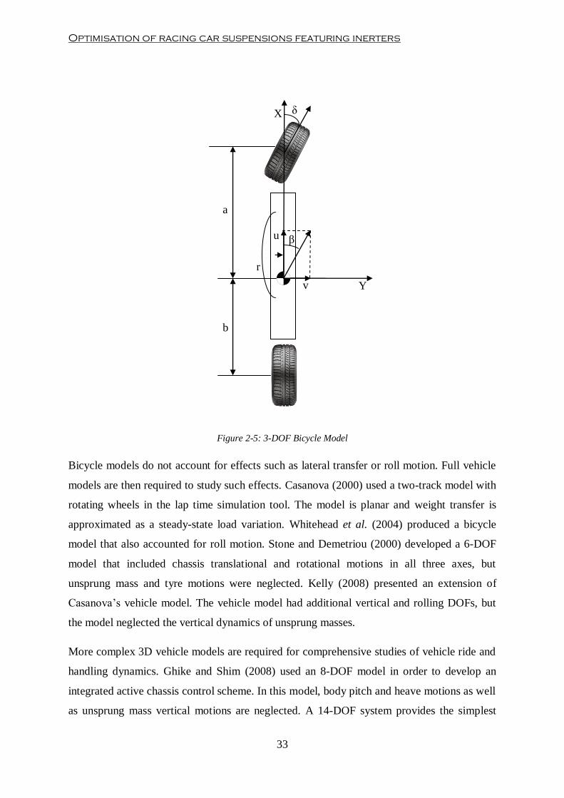
Optimisation of racing car suspensions featuring inerters
33
Figure 2-5: 3-DOF Bicycle Model
Bicycle models do not account for effects such as lateral transfer or roll motion. Full vehicle
models are then required to study such effects. Casanova (2000) used a two-track model with
rotating wheels in the lap time simulation tool. The model is planar and weight transfer is
approximated as a steady-state load variation. Whitehead et al. (2004) produced a bicycle
model that also accounted for roll motion. Stone and Demetriou (2000) developed a 6-DOF
model that included chassis translational and rotational motions in all three axes, but
unsprung mass and tyre motions were neglected. Kelly (2008) presented an extension of
Casanova’s vehicle model. The vehicle model had additional vertical and rolling DOFs, but
the model neglected the vertical dynamics of unsprung masses.
More complex 3D vehicle models are required for comprehensive studies of vehicle ride and
handling dynamics. Ghike and Shim (2008) used an 8-DOF model in order to develop an
integrated active chassis control scheme. In this model, body pitch and heave motions as well
as unsprung mass vertical motions are neglected. A 14-DOF system provides the simplest
u
v Y
X
a
b
δ
β
r

Chapter 2- Literature Review
34
representation of a full-car vehicle model (March & Shim, 2007). Such a model account
includes translational and rotational body motions (6 DOFs) and vertical and rotational
motion at each wheel (two additional DOFs per wheel). Shim and Ghike (2007) presented a
comparative study of the accuracy of different vehicle models. In this work, a comprehensive
nonlinear 14-DOF full vehicle model was developed first and simplifying assumptions were
then gradually introduced into the model. Differences among vehicle models were analysed
in order to compare the impact of modelling simplifications in the dynamic response of the
vehicle.
2.7.4. Lap Time Simulation as part of Suspension Optimisation Algorithm
As mentioned in the previous section, the outcome of a suspension multi-objective
optimisation is a set of non-dominated optimal solutions (Deb, 2001). In motor racing, since
only passive suspensions are allowed by the governing body, one single solution from the
optimal set must be selected. Higher order information is required to select the specific
solution that will suit a particular situation. So, in order to choose among the Pareto-optimal
solution set, a decision-maker tool is required. In vehicle suspension design and optimisation,
a decision-maker is composed of a set of performance metrics that will weight the different
objective functions so that a final solution can be obtained. In Motorsport, the ultimate goal
of vehicle system is to obtain a configuration such that the time taken to complete a lap
around a race track could be minimised. Modifications in suspension settings have an
important impact on the performance of the car and, ultimately, on its lap time. According to
this, higher order information will come from the study of the impact of suspension changes
in the overall performance of a race car. The higher order information could be obtained from
two different approaches: on-track testing and lap-time simulation. Due to the competitive
nature of Motorsport, no relevant data have been published with regard to the impact of
suspension changes in the actual on-track performance of a race car. Moreover, developing a
decision maker based on track testing would involve the construction of a fully operative race
car prototype. Although information obtained from this type of testing is invaluable, the costs
involved and the limited number of tests allowed by governing body make this option
unviable in most cases. A much more cost-effective option for the development of a decision
maker tool can be found in the analysis of suspensions in the overall vehicle performance via
lap-time simulation.
Optimisation of racing car suspensions featuring inerters
35
Although it has been already stated that changes in the suspension will have an impact on
vehicle handling characteristics and on overall vehicle performance (Benedetti, et al., 2006;
Blank & Margolis, 1996; Floyd & Law, 1994), only a few reported studies have been found
in literature with regard to the analysis of the impact of a race car suspensions on one-lap
performance. Kelly (2008) presented a study of a race car transient cornering manoeuvres. In
this study, an idealised vehicle suspension with decoupled heave and roll modes was
proposed, and the effect of heave and roll stiffness and damping was analysed for different
corner layouts. However, there are no reported studies in literature that make use of lap-time
simulators as higher order information decision makers in the suspension optimisation
process.
2.8. Summary
A review of the significant literature for this research work has been presented in this chapter.
The first section introduces the importance of suspension in racing cars. A brief historical
background of the evolution of race car suspension technology has been reviewed and the
importance of suspension design and optimisation has been highlighted.
The inerter concept and its potential applications have been presented. The definition of an
ideal inerter has been introduced and the different design solutions available in literature have
been discussed. Moreover, reported studies of potential benefits in field of ground vehicle
suspensions, motorcycle steering systems and building technology have been discussed.
Experimental inerter studies have been also covered. The review presented on this area
revealed that experimental inerters have only been tested in isolation to other suspension
components.
In section 2.4, experimental testing techniques for the dynamic analysis of vehicle suspension
have been discussed. The main characteristics of post rig test facilities have been discussed,
and examples of their use in literature have been provided. No reported studies consider the
analysis of suspension featuring inerters using these facilities.
A section dedicated to reviewing virtual suspension modelling and simulation has also been
covered. A review of different suspension models has been carried out. Model complexity
and applications in simulation and optimisation have been discussed. Although research
studies devoted to modelling and validation of individual inerters devices have been found,

Chapter 2- Literature Review
36
no literature that proposes a complete and validated vehicle suspension model that includes
real inerters has been reported.
Suspension optimisation is a key factor in vehicle performance. Section 2.6 covered different
aspects in suspension optimisation. Firstly, a review of suspension objectives reported in
literature has been carried out. Secondly, different optimisation algorithms applied to
suspension technology have been presented. Optimisation methods have been reviewed with
respect to the requirements for suspension optimisation. Finally, methods for increasing the
efficiency and robustness of optimisation algorithms have been described. However, no
studies have been found in literature that produced an objective performance-based
suspension optimisation methodology that reflects the impact of ride dynamics on handling
characteristic and on the performance of a race car.
The last section of chapter 2 was dedicated to lap-time simulation. The concept and
importance of lap-time simulation in motor racing has been presented. Different lap time
simulation strategies have been described and the most relevant work in this field has been
critically reviewed. Furthermore, a review of vehicle models for simulation has been carried
out. Different full vehicle models have been discussed. No reported studies that use lap-time
simulation as a decision maker in a suspension optimisation problem have been found.
Chapter 2 sets out the state-of-the art of engineering and technology in the research areas
related to the work developed in this thesis and it highlights the gaps in existing work related
to optimisation of racing car suspensions featuring inerters.
Optimisation of racing car suspensions featuring inerters
37
3. Theoretical Analysis of Ideal Inerters in Vibratory Systems
3.1. Introduction
The simplest model in the analysis of dynamic vibratory systems can be described as a single
degree-of-freedom (SDOF) rigid mass, elastically connected to a base or some form of
excitation. The system is termed SDOF because the mass is only allowed to move in one
direction.
SDOF models can provide relevant information about the system regardless of their
simplicity. Furthermore, due to this simplicity, these models have been widely used in many
applications such as bridges, buildings, aerospace structures, mechanical engineering and so
on. The results obtained from the analysis of a SDOF system can be used as the foundation
for the development of more complex models.
The study and analysis of these models has been widely covered in literature and Dynamics
textbooks. However, there is no record in the literature that characterises and analyses the
effect of inertial damping in the dynamic behaviour of such systems. First of all, an ideal
inerter can be defined as a mechanical device in which the force applied to its terminals is
proportional to the relative acceleration between these nodes (Smith, 2002). According to this
definition, the characteristic equation of an (ideal) inerter, as described in section 2.3, is:
Where F is the equal and opposite force applied at each terminal, ai represents the absolute
acceleration at the ith
node and b represents inertance and has units of kilograms in SI.
In this chapter, the property of an ideal ball screw inerter has been defined. Furthermore, an
ideal inerter modelled as a SDOF is analysed for un-damped and damped cases. Equations of
motion of the system are derived and analytical solutions are given in free and forced
vibration situations. The effect of inerters and its interaction with other elastic components
are analysed. Results of this analysis set the foundation for the development of more complex
vibratory systems.
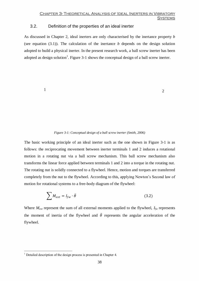
Chapter 3- Theoretical Analysis of Ideal Inerters in Vibratory
Systems
38
3.2. Definition of the properties of an ideal inerter
As discussed in Chapter 2, ideal inerters are only characterised by the inertance property b
(see equation (3.1)). The calculation of the inertance b depends on the design solution
adopted to build a physical inerter. In the present research work, a ball screw inerter has been
adopted as design solution1. Figure 3-1 shows the conceptual design of a ball screw inerter.
Figure 3-1: Conceptual design of a ball screw inerter (Smith, 2006)
The basic working principle of an ideal inerter such as the one shown in Figure 3-1 is as
follows: the reciprocating movement between inerter terminals 1 and 2 induces a rotational
motion in a rotating nut via a ball screw mechanism. This ball screw mechanism also
transforms the linear force applied between terminals 1 and 2 into a torque in the rotating nut.
The rotating nut is solidly connected to a flywheel. Hence, motion and torques are transferred
completely from the nut to the flywheel. According to this, applying Newton’s Second law of
motion for rotational systems to a free-body diagram of the flywheel:
Where Mext represent the sum of all external moments applied to the flywheel, Ifw represents
the moment of inertia of the flywheel and represents the angular acceleration of the
flywheel.
1 Detailed description of the design process is presented in Chapter 4.
1 2
Optimisation of racing car suspensions featuring inerters
39
Due to the coupling between translational and rotational movement, translational force at the
device terminals, F, and torque transmitted to the flywheel, T, are related by the following
expression:
Where l represents the lead of the screw, F represents the translational force at the device
terminals.
In the same way as above, translational relative displacement of the device terminals (x(t)) is
related to the angular rotation of the flywheel, θ, as follows:
Introducing equations (3.3) and (3.4) into equation (3.2), the following expression is
obtained:
Recalling that the representation of an ideal inerter is (see equation (3.1)), the
inertance of a ball screw mechanism can be obtained as:
Where b represents the inertance of the inerter expressed in kg and arel represents the
translational relative acceleration between inerter terminals.
3.3. Analysis of an un-damped Inerter modelled as a SDOF
The simplest model in engineering vibration is a single degree-of-freedom (SDOF) system
that does not account for damping effects – un-damped case. Such a model is depicted in
Figure 3-2.

Chapter 3- Theoretical Analysis of Ideal Inerters in Vibratory
Systems
40
Figure 3-2: Un-damped SDOF system with inerter
In the conventional SDOF model, the solid-rigid mass is connected elastically via an ideal
spring to a base or excitation. Only translational motion in vertical direction has been
considered as a degree of freedom. In this study, an ideal inerter is connected in parallel with
the spring. In order to obtain the equation of motion of the system depicted in Figure 3-2,
Newton’s Second law of Mechanics has been applied to the free-body diagram of this system.
(3.7)
Equation (3.7) represents the motion of the mass M subjected to the force of the spring and
the inerter, gravity and external forces applied to the mass; x(t) and its derivatives represent
the movement (displacement, velocity and acceleration) of the mass M and z(t) and its
derivatives represents the movement of the base. Note that, for simplicity in the notation,
x(t)=x.
Assuming that the system at t=0 is in equilibrium and no external forces are applied to the
mass, equation (3.7) can be rearranged as follows:
(3.8)
Where (3.8) is a second-order ordinary differential equation (ODE). Assuming that, the input
of the base excitation is a sinusoidal waveform (forced excitation), equation (3.8) can be
solved by applying Laplace transform to both sides of the equation:
Optimisation of racing car suspensions featuring inerters
41
(3.9)
Where s represents the Laplace operator. In systems subjected to sinusoidal inputs s=jω,
where j is the imaginary number and ω is the angular frequency and x(0) and v(0) represent
the initial conditions (displacement and velocity) of the system.
Note that, by applying the Laplace transform to the equation (3.8), the resulting equation
(3.9) is now second-order algebraic equation that can be solved easily.
For simplicity in the solution, the initial conditions of mass M have been set equal to 0.
According to this, the transmissibility function of the system G(s), i.e. the ratio between the
output and the input, has been defined as:
Or in terms of angular frequency:
Eq. (3.11) represents the frequency response function (FRF) of an un-damped SDOF system
fitted with an inerter. This equation represents the frequency domain of a system under forced
vibration.
In addition to this, a non-dimensional parameter χ can be defined in order to express the
inertance b in terms of the mass of the system M:
By introducing expression (3.12) into equation (3.11), the following expression has been
obtained:

Chapter 3- Theoretical Analysis of Ideal Inerters in Vibratory
Systems
42
Note that, even though, due to the nature of the system, no imaginary part exists, equation
(3.13) can still be expressed in complex notation z=a+bj, where a is the real part, b is the
imaginary part and j is the imaginary number. According to this, the magnitude and phase of
a complex number can be obtained as follows:
According to this, the amplitude and phase angle response for an un-damped single DOF with
inerter can be expressed as follows:
Equations (3.16) and (3.17) can be therefore used to determine the response of the system and
to analyse the impact of the inerters in this response. A set of mechanical properties must be
set in order to obtain the analytical solution of the system. Table 3-1 shows the mechanical
parameters selected in this study.
These mechanical parameters have been introduced into equations (3.16) and (3.17), so that
the effect of inerters in the amplitude ratio and phase responses of the SDOF system can be
analysed. Figure 3-3 depicts the response of an un-damped SDOF system for different values
of inertance.
Mass (M) 100 kg
Spring stiffness (k) 20000 N/m
Inertance tuning range (b) [0-120] kg
Frequency range (f) [0-20] Hz
Table 3-1: Mechanical properties of the un-damped SDOF system
Note that, although the frequency range of study is from 0 to 20 Hz, the plot only shows the
first 10 Hz for clarity. The y-axis has been limited due to the fact that, at the natural
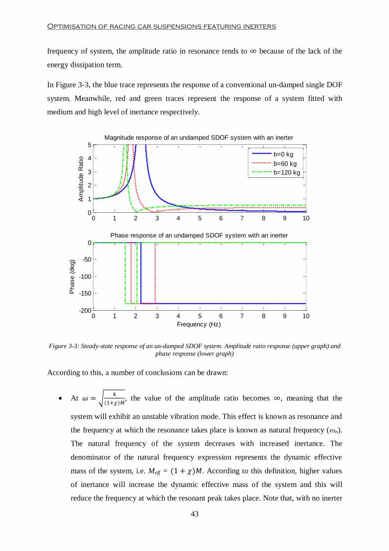
Optimisation of racing car suspensions featuring inerters
43
frequency of system, the amplitude ratio in resonance tends to because of the lack of the
energy dissipation term.
In Figure 3-3, the blue trace represents the response of a conventional un-damped single DOF
system. Meanwhile, red and green traces represent the response of a system fitted with
medium and high level of inertance respectively.
Figure 3-3: Steady-state response of an un-damped SDOF system. Amplitude ratio response (upper graph) and
phase response (lower graph)
According to this, a number of conclusions can be drawn:
At
, the value of the amplitude ratio becomes , meaning that the
system will exhibit an unstable vibration mode. This effect is known as resonance and
the frequency at which the resonance takes place is known as natural frequency (ωn).
The natural frequency of the system decreases with increased inertance. The
denominator of the natural frequency expression represents the dynamic effective
mass of the system, i.e. Meff = . According to this definition, higher values
of inertance will increase the dynamic effective mass of the system and this will
reduce the frequency at which the resonant peak takes place. Note that, with no inerter
0 1 2 3 4 5 6 7 8 9 100
1
2
3
4
5Magnitude response of an undamped SDOF system with an inerter
Am
plit
ude R
atio
b=0 kg
b=60 kg
b=120 kg
0 1 2 3 4 5 6 7 8 9 10-200
-150
-100
-50
0Phase response of an undamped SDOF system with an inerter
Frequency (Hz)
Phase (
deg)
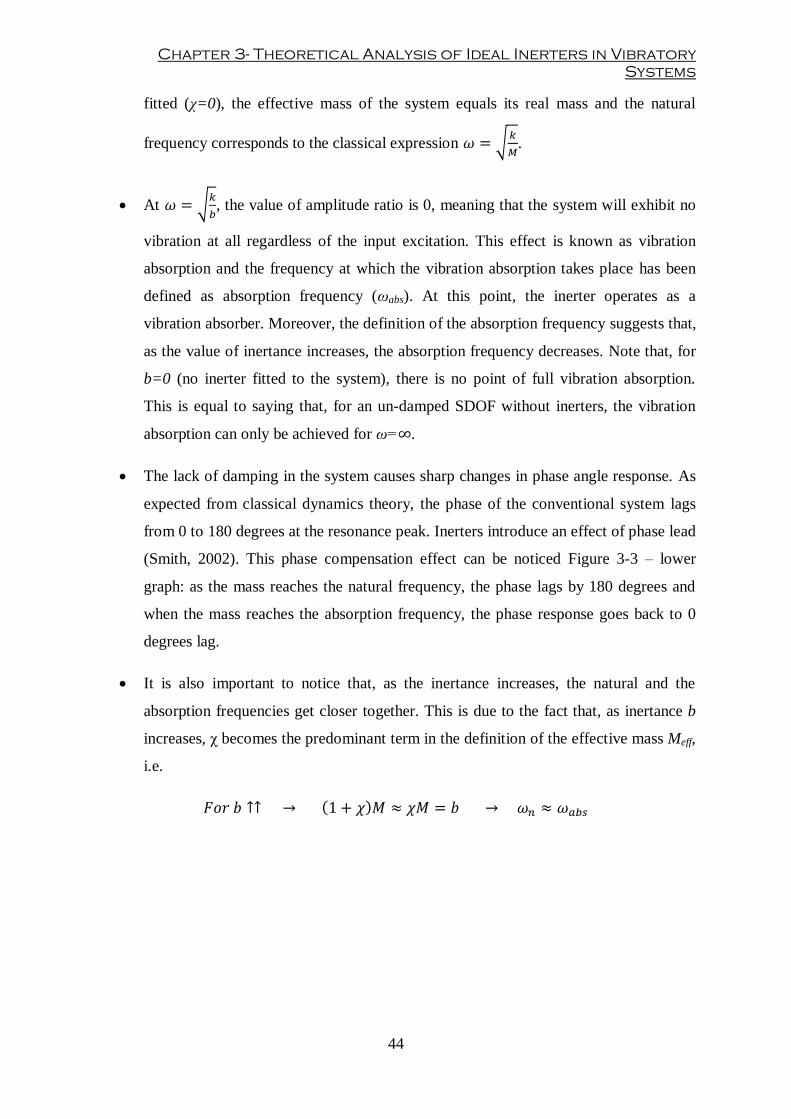
Chapter 3- Theoretical Analysis of Ideal Inerters in Vibratory
Systems
44
fitted (χ=0), the effective mass of the system equals its real mass and the natural
frequency corresponds to the classical expression
.
At
, the value of amplitude ratio is 0, meaning that the system will exhibit no
vibration at all regardless of the input excitation. This effect is known as vibration
absorption and the frequency at which the vibration absorption takes place has been
defined as absorption frequency (ωabs). At this point, the inerter operates as a
vibration absorber. Moreover, the definition of the absorption frequency suggests that,
as the value of inertance increases, the absorption frequency decreases. Note that, for
b=0 (no inerter fitted to the system), there is no point of full vibration absorption.
This is equal to saying that, for an un-damped SDOF without inerters, the vibration
absorption can only be achieved for ω= .
The lack of damping in the system causes sharp changes in phase angle response. As
expected from classical dynamics theory, the phase of the conventional system lags
from 0 to 180 degrees at the resonance peak. Inerters introduce an effect of phase lead
(Smith, 2002). This phase compensation effect can be noticed Figure 3-3 – lower
graph: as the mass reaches the natural frequency, the phase lags by 180 degrees and
when the mass reaches the absorption frequency, the phase response goes back to 0
degrees lag.
It is also important to notice that, as the inertance increases, the natural and the
absorption frequencies get closer together. This is due to the fact that, as inertance b
increases, χ becomes the predominant term in the definition of the effective mass Meff,
i.e.

Optimisation of racing car suspensions featuring inerters
45
3.4. Analysis of a Damped Inerter modelled as a SDOF
The analysis of the un-damped case has been helpful in understanding the basics of the
inerter behaviour. However, in most real-life engineering applications a certain level of
energy dissipation must be assumed. For fundamental vibration analysis, an ideal damper can
be assumed to model this energy dissipation term. In this section, damping effects have been
included in the study of the inerters in vibratory systems. Therefore, the SDOF presented in
the previous section has been extended in order to account for the damping component.
Figure 3-4 shows a schematic representation of a damped SDOF system fitted with inerters.
Figure 3-4: Damped SDOF system with inerter
Following the same procedure as in the previous section, the equation of motion of the
system has been derived by applying Newton 2nd
Law of Mechanics to the free-body diagram
of the system:
Assuming that the system is in equilibrium at the beginning of the motion and no external
forces have been applied to the mass, the previous equation of motion can be re-arranged into
the following second-order ordinary differential equation:

Chapter 3- Theoretical Analysis of Ideal Inerters in Vibratory
Systems
46
Equation (3.19) has been translated into an algebraic equation by using the Laplace transform
as follows:
Equation (3.20) represents the behaviour of a general single DOF system that accounts for
both damping and inertial effects expressed in terms of the Laplace operator. From this
equation, both the steady-state and transient responses of the system have been derived.
In the following sections of this chapter, the steady-state amplitude ratio and the phase angle
response subjected to a forced excitation has been analysed in the frequency domain.
Furthermore, the transient response of the system has been studied by obtaining the analytical
expression of mass displacement x(t) in the time domain.
3.4.1. Analysis in the frequency domain
As in section 3.3, initial conditions of displacement and velocity have been considered to be
0, so equation (3.20) can be rewritten as follows:
Laplace operator s has been substituted by the frequency term in order to obtain G(w). By
applying equations (3.14) and (3.15) to G(w), amplitude ratio and phase angle frequency
domain responses have been obtained:
As discussed in section 3.3, a set of mechanical parameters must be provided in order to
obtain the amplitude ratio and phase angle response of the system (see Table 3-2).
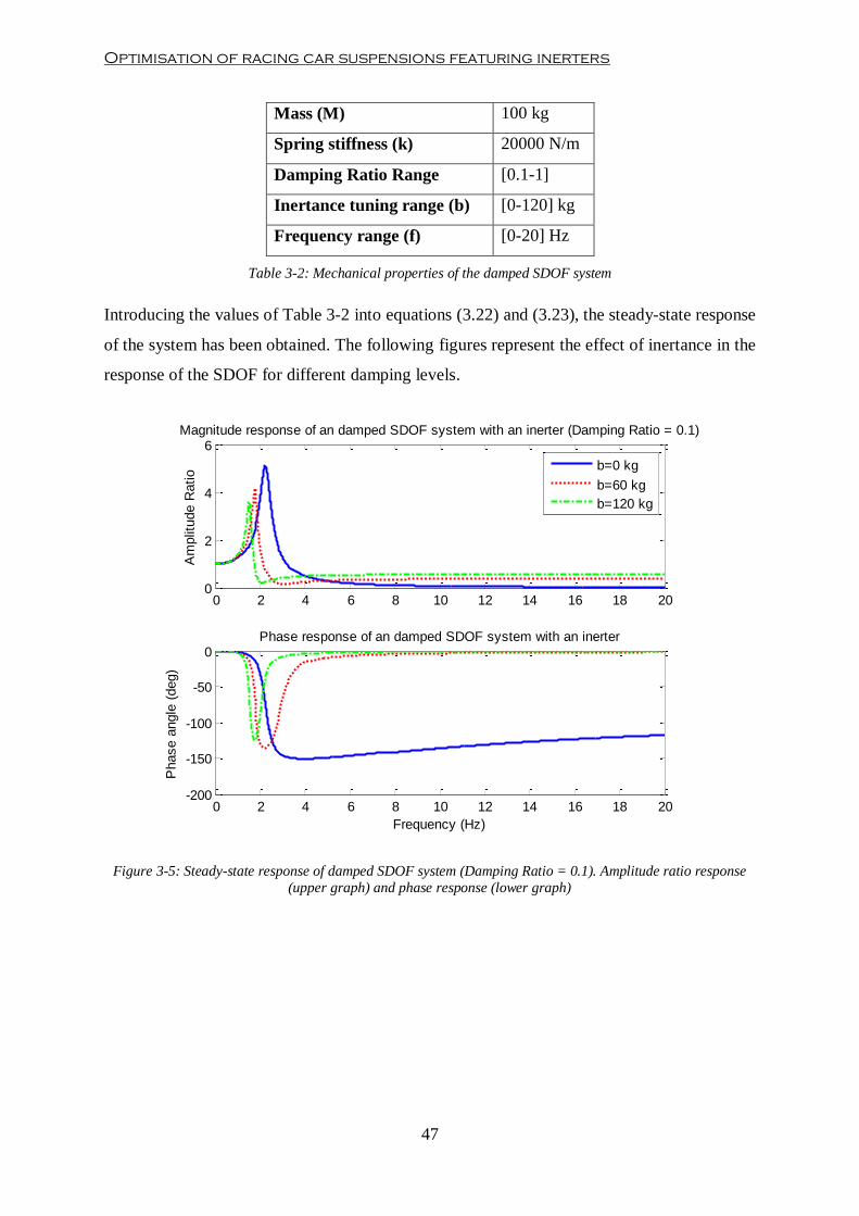
Optimisation of racing car suspensions featuring inerters
47
Mass (M) 100 kg
Spring stiffness (k) 20000 N/m
Damping Ratio Range [0.1-1]
Inertance tuning range (b) [0-120] kg
Frequency range (f) [0-20] Hz
Table 3-2: Mechanical properties of the damped SDOF system
Introducing the values of Table 3-2 into equations (3.22) and (3.23), the steady-state response
of the system has been obtained. The following figures represent the effect of inertance in the
response of the SDOF for different damping levels.
Figure 3-5: Steady-state response of damped SDOF system (Damping Ratio = 0.1). Amplitude ratio response
(upper graph) and phase response (lower graph)
0 2 4 6 8 10 12 14 16 18 200
2
4
6Magnitude response of an damped SDOF system with an inerter (Damping Ratio = 0.1)
Am
plit
ude R
atio
b=0 kg
b=60 kg
b=120 kg
0 2 4 6 8 10 12 14 16 18 20-200
-150
-100
-50
0Phase response of an damped SDOF system with an inerter
Frequency (Hz)
Phase a
ngle
(deg)
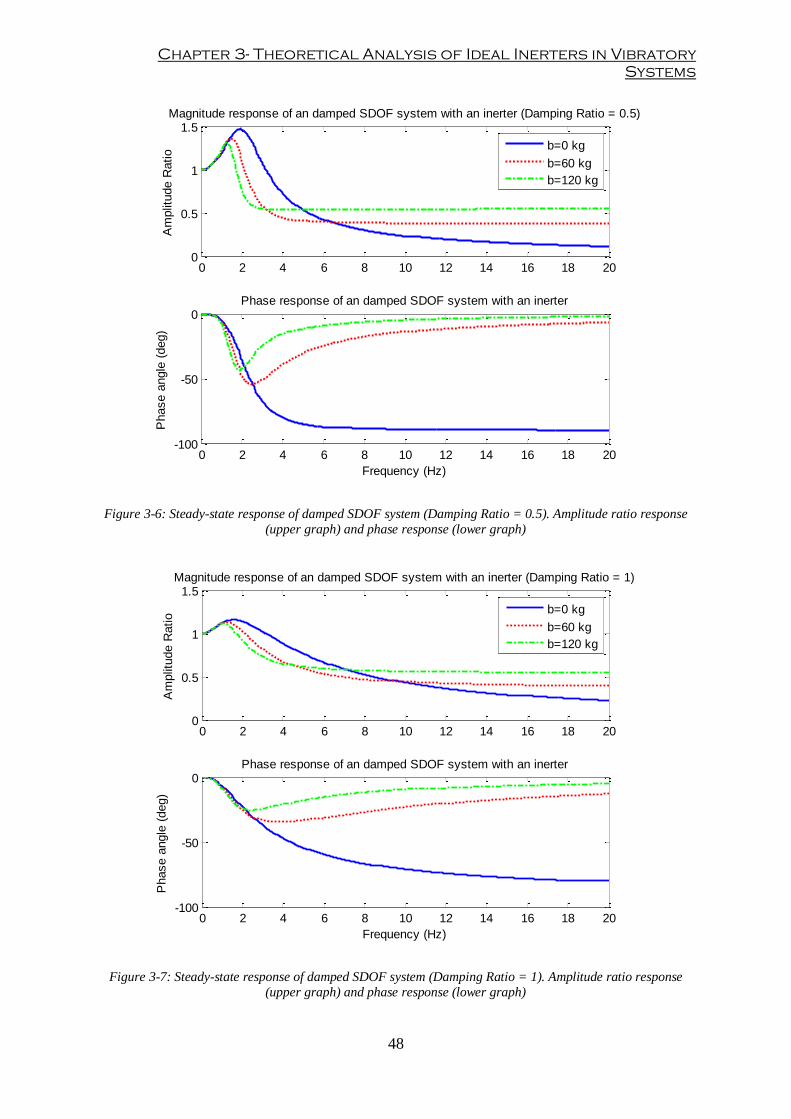
Chapter 3- Theoretical Analysis of Ideal Inerters in Vibratory
Systems
48
Figure 3-6: Steady-state response of damped SDOF system (Damping Ratio = 0.5). Amplitude ratio response
(upper graph) and phase response (lower graph)
Figure 3-7: Steady-state response of damped SDOF system (Damping Ratio = 1). Amplitude ratio response
(upper graph) and phase response (lower graph)
0 2 4 6 8 10 12 14 16 18 200
0.5
1
1.5Magnitude response of an damped SDOF system with an inerter (Damping Ratio = 0.5)
Am
plit
ude R
atio
b=0 kg
b=60 kg
b=120 kg
0 2 4 6 8 10 12 14 16 18 20-100
-50
0Phase response of an damped SDOF system with an inerter
Frequency (Hz)
Phase a
ngle
(deg)
0 2 4 6 8 10 12 14 16 18 200
0.5
1
1.5Magnitude response of an damped SDOF system with an inerter (Damping Ratio = 1)
Am
plit
ude R
atio
b=0 kg
b=60 kg
b=120 kg
0 2 4 6 8 10 12 14 16 18 20-100
-50
0Phase response of an damped SDOF system with an inerter
Frequency (Hz)
Phase a
ngle
(deg)
Optimisation of racing car suspensions featuring inerters
49
Firstly, Figure 3-5 to Figure 3-7 show that the effect of an inerter in a SDOF system is similar
regardless of the level of damping of the system. More inertance translates into an increase in
the dynamic effective mass of the system, which, in turn, reduces both the natural frequency
and the amplitude of the resonant peak. As expected, increasing damping helps to smooth the
steady-state response of the system. Higher levels of damping contribute to a better controlled
resonant mode, i.e. lower values of amplitude ratio around the natural frequency.
As in the un-damped case, the inerter acts as a vibration absorber. However, in this case, the
damping term causes a reduction this absorption effect. Note that, with a damping ratio of 0.1
(see Figure 3-5), the decrease of the amplitude ratio at ωabs is quite noticeable. However, the
vibration absorption effect can be barely noticed for higher damping ratios (see Figure 3-6
and Figure 3-7). This is due to fact that increases in damping reduce the relative motion of the
suspension (“locking-up” effect).
Moreover, at high frequencies, the amplitude ratio tends to
regardless of the level of
damping of the system. This effect is caused because the inerter is connected to both the input
(base) and the output (mass). As shown in the un-damped case, inerters introduce a phase
lead on the system. This phase lead causes the mass to catch up with the input excitation back
again after initial phase lag. Phase angle response plots show that the phase compensation is
more effective for higher values of inertance. This, in turn, allows the output to match more
effectively the input, hence, the amplitude ratio at higher frequencies gets closer to 1. In the
limit, very high levels of inertance, phase compensation would be 100% effective, leading to
a perfect match between input and output signals, i.e. an amplitude ratio equals to 1. On the
other hand, higher levels of damping contribute to slowing down this phase compensation
(see Figure 3-7), reducing the effectiveness of the output to catch up with the input.
Some conclusions can be drawn from this frequency domain analysis: on one hand, higher
inertance values could be beneficial at low frequencies (ω ≈ ωn) due to the fact that, for the
same spring value k, the effective frequency response corresponds to the one of a softer
system, i.e. lower amplitude at the body mode and lower natural frequency. Lower
transmissibility at low frequencies improves body control. However, on the other hand, at
high frequencies (ω > ωn), lower values of inertance could be more beneficial, due to the
increased transmissibility caused by high inerter values. Therefore, high inertance will cause
poorer vibration isolation at frequencies over the natural frequency ωn. This suggests that a
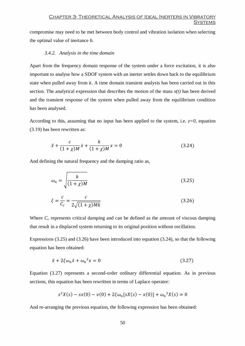
Chapter 3- Theoretical Analysis of Ideal Inerters in Vibratory
Systems
50
compromise may need to be met between body control and vibration isolation when selecting
the optimal value of inertance b.
3.4.2. Analysis in the time domain
Apart from the frequency domain response of the system under a force excitation, it is also
important to analyse how a SDOF system with an inerter settles down back to the equilibrium
state when pulled away from it. A time domain transient analysis has been carried out in this
section. The analytical expression that describes the motion of the mass x(t) has been derived
and the transient response of the system when pulled away from the equilibrium condition
has been analysed.
According to this, assuming that no input has been applied to the system, i.e. z=0, equation
(3.19) has been rewritten as:
And defining the natural frequency and the damping ratio as,
Where Cc represents critical damping and can be defined as the amount of viscous damping
that result in a displaced system returning to its original position without oscillation.
Expressions (3.25) and (3.26) have been introduced into equation (3.24), so that the following
equation has been obtained:
Equation (3.27) represents a second-order ordinary differential equation. As in previous
sections, this equation has been rewritten in terms of Laplace operator:
And re-arranging the previous equation, the following expression has been obtained:

Optimisation of racing car suspensions featuring inerters
51
In order to obtain the analytical solution of the transient response of the SDOF, the roots of
the denominator equation (also known as characteristic equation) can be obtained and
equation (3.28) can be re-arranged according to the value of the roots of this characteristic
equation. Moreover, the value of these roots depends on the value of the damping ratio .
According to this, three different cases can be distinguished: under-damped, critically
damped and over-damped cases. For each of these cases, equation (3.28) can be re-arranged
into a different expression. These re-arranged equations can then be solved by means of
Inverse Laplace transform.
Under-damped case ( :
The denominator of eq. (3.28) can be rewritten as follows:
Where is the damped natural frequency.
If the new expression for the denominator is introduced in equation (3.28) and some re-
arrangements are made to the equation, the following expression can be obtained:
And by applying inverse Laplace transform to equation (3.29), the analytical expression for
mass displacement can be obtained as:
Equation (3.30) represents an oscillatory system, due to the sinusoidal terms, with a
logarithmic decrement in the amplitude of vibration. Note that, expressions for mass velocity
and acceleration with respect to time can be readily derived from equation (3.30) by using
common time differentiation.

Chapter 3- Theoretical Analysis of Ideal Inerters in Vibratory
Systems
52
Critically damped case ( ):
In this special case, the damped natural frequency is equal to 0 and equation (3.29) can be
rewritten as follows:
By applying again inverse Laplace transform to the equation (3.31), the analytical solution
for a critically damped case can be obtained as follows:
Expression (3.32) shows that the response of the system does not present an oscillatory
behaviour due to the lack of sinusoidal terms. Instead, the response of the system to free-
vibration non-zero initial condition would logarithmically decay to the equilibrium point.
Over-damped case ( ):
The solution process for this case is much longer and tedious than in the other two cases. So,
for brevity and clarity of the section, only the final time-domain expression for displacement
has been presented.
Where
As in the previous case, equation (3.33) represents an exponential decay to the equilibrium
condition. However in this case, the decay is slower than in a critically damped system due to
the factor added to the exponential function.
Equations (3.30), (3.32) and (3.33) represent the transient response of a damped SDOF
system incorporating an ideal inerter subject to a non-zero initial condition. In this section,
the initial conditions considered to run the study are presented in the following table:

Optimisation of racing car suspensions featuring inerters
53
Initial displacement x(0) 0.2 m
Initial velocity v(0) 0 m/s
Table 3-3: Initial conditions for transient analysis
By setting these initial conditions, a system being subjected to a step input of amplitude 20
cm at t=0 sec can be simulated.
Two different tests have been run: the first one, in the under-damped region; and the second
one, in the transition from over-damped to under-damped region. In order to do so, two
different values of damping coefficient have been set.
Test Damping Coefficient
Under-damped 1000 N/m/s
Transition 3465 N/m/s
Table 3-4: Damping coefficients used in simulation
For each of these tests, three different levels of inertance have been applied to study the effect
of inerters in the transient behaviour of the system. Figure 3-8 and Figure 3-9 show the
transient response for an under-damped and a near critically damped system respectively.
Figure 3-8: Transient response of the system in the under-damped region
0 0.2 0.4 0.6 0.8 1 1.2 1.4 1.6 1.8 2-0.1
-0.05
0
0.05
0.1
0.15
0.2
0.25Free vibration SDOF system featuring inerters x0=0.2m and c=1000Nm/s
time (secs)
Dis
pla
cem
ent
(m)
b=0 kg
b=60 kg
b=120 kg
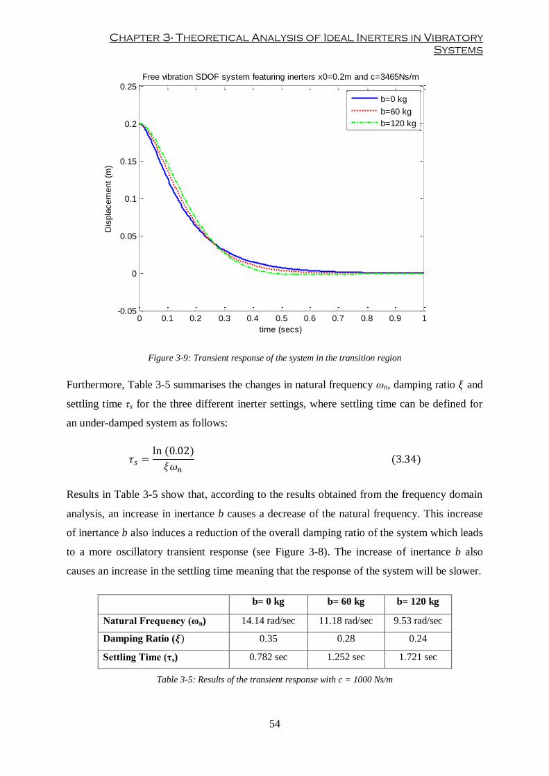
Chapter 3- Theoretical Analysis of Ideal Inerters in Vibratory
Systems
54
Figure 3-9: Transient response of the system in the transition region
Furthermore, Table 3-5 summarises the changes in natural frequency ωn, damping ratio and
settling time τs for the three different inerter settings, where settling time can be defined for
an under-damped system as follows:
Results in Table 3-5 show that, according to the results obtained from the frequency domain
analysis, an increase in inertance b causes a decrease of the natural frequency. This increase
of inertance b also induces a reduction of the overall damping ratio of the system which leads
to a more oscillatory transient response (see Figure 3-8). The increase of inertance b also
causes an increase in the settling time meaning that the response of the system will be slower.
b= 0 kg b= 60 kg b= 120 kg
Natural Frequency (ωn) 14.14 rad/sec 11.18 rad/sec 9.53 rad/sec
Damping Ratio ( 0.35 0.28 0.24
Settling Time (τs) 0.782 sec 1.252 sec 1.721 sec
Table 3-5: Results of the transient response with c = 1000 Ns/m
0 0.1 0.2 0.3 0.4 0.5 0.6 0.7 0.8 0.9 1-0.05
0
0.05
0.1
0.15
0.2
0.25Free vibration SDOF system featuring inerters x0=0.2m and c=3465Ns/m
time (secs)
Dis
pla
cem
ent
(m)
b=0 kg
b=60 kg
b=120 kg
Optimisation of racing car suspensions featuring inerters
55
Table 3-6 summarises the changes in natural frequency ωn, damping ratio and for the three
different inerter settings in the near critically damped case study. Results from Figure 3-9 and
Table 3-6 show that, as in the previous case study, both natural frequency ωn and damping
ratio decrease as inertance b increases. In this case, additional inertance on the system has
changed the over-damped response to an under-damped response.
b= 0 kg b= 60 kg b= 120 kg
Natural Frequency (ωn) 14.14 rad/sec 11.18 rad/sec 9.53 rad/sec
Damping Ratio ( 1.22 0.97 0.83
Table 3-6: Results of the transient response with c = 3465 Ns/m
3.4.3. Study of sensitivity
The final part of this section has been devoted to studying the behaviour between an inerter
and a damper. In order to do so, sensitivity study has been carried out. The variable of study
in the sensitivity analysis is the overall damping ratio of the system. The nominal parameters
used in this study are presented in Table 3-7.
Mass (M) 100 kg
Spring stiffness (k) 20000 N/m
Damping Coefficient (c) 3465 N/m/s
Inertance (b) 50 kg
Table 3-7: Parameters used for sensitivity analysis
The parameters from Table 3-7 have been chosen so that the initial damping ratio is equal to
1. Damping and inertance values have been swept in a range of ±50% from their nominal
values and overall damping ratio has been obtained.
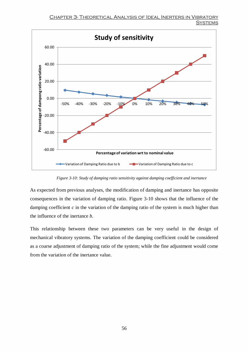
Chapter 3- Theoretical Analysis of Ideal Inerters in Vibratory
Systems
56
Figure 3-10: Study of damping ratio sensitivity against damping coefficient and inertance
As expected from previous analyses, the modification of damping and inertance has opposite
consequences in the variation of damping ratio. Figure 3-10 shows that the influence of the
damping coefficient c in the variation of the damping ratio of the system is much higher than
the influence of the inertance b.
This relationship between these two parameters can be very useful in the design of
mechanical vibratory systems. The variation of the damping coefficient could be considered
as a coarse adjustment of damping ratio of the system; while the fine adjustment would come
from the variation of the inertance value.
-60.00
-40.00
-20.00
0.00
20.00
40.00
60.00
-50% -40% -30% -20% -10% 0% 10% 20% 30% 40% 50%
Pe
rce
nta
ge o
f d
amp
on
g ra
tio
var
iati
on
Percentage of variation wrt to nominal value
Study of sensitivity
Variation of Damping Ratio due to b Variation of Damping Ratio due to c

Optimisation of racing car suspensions featuring inerters
57
3.5. Summary
The aim of this chapter was to study and analyse the effect of ideal inerters in simple
vibratory mechanical systems, prior to considering how these can be realised and how they
behave in practical systems. Section 3.2 defined the inertance characteristics of an ideal ball
screw mechanical inerter. Section 3.3 introduced the equations of motion for an un-damped
SDOF system fitted with inerters under forced vibration situation and a steady-state analysis
has been carried out in order to outline the basic properties of an ideal inerter in simple
vibratory systems. In section 3.4, this study has been generalised for a system that accounted
for damping effects. Steady-state and transient responses have been analysed for a range of
damping and inertance values. Finally, a sensitivity analysis has been carried out in order to
study the relative impact of inerters in the overall damping ratio of a vibratory system.
Several conclusions can be drawn from this chapter:
Increasing the value of inertance causes a decrease in both the natural frequency of the
system ωn and the amplitude A(ω) at the resonant peak. This is due to an increase in the
dynamic effective mass Meff=M+b of the system.
The addition of an ideal inerter in an un-damped system causes a phenomenon of
vibration absorption. The frequency at which this phenomenon takes place is known as
the absorption frequency ωabs. In the damped case, this phenomenon still persists.
However, higher values of damping lead to a decrease of the vibration absorption
effectiveness.
Phase lead is an important characteristic introduced by the use of inerters. This
characteristic helps to compensate the phase lag experienced by the system as it reaches
its resonant frequency. Higher values of inertance increase the effectiveness of the phase
compensation.
Frequency domain analysis suggests that a higher value of inertance is beneficial at low
frequencies (around the ωn) and can be desirable because it offers an enhanced body
mode control and, to some extent, depending on damping, a vibration absorption effect.
However, at high frequencies (far away from the ωn), lower values of inertance would be
more beneficial. Low inertance values will promote better vibration isolation at high
frequencies.
Chapter 3- Theoretical Analysis of Ideal Inerters in Vibratory
Systems
58
Transient analysis suggests that increased inertance values reduce the effective damping
ratio of the system. This study suggests that inerters could be used to fine tune the
transient characteristics of a system.
Sensitivity studies reveal that tuning the damping coefficient and the inertance value have
opposing consequences in the damping ratio. The impact of damping variation in the
effective damping ratio is larger than the impact of inertance variations.
This chapter has characterised the behaviour of simple ideal dynamic systems fitted with
inerters. The characteristic response in frequency and time domain of a SDOF system with
and without damping effects has been obtained. The study carried out in this chapter sets the
foundation above which a novel vehicle suspension model incorporating real mechanical
inerters has been developed.
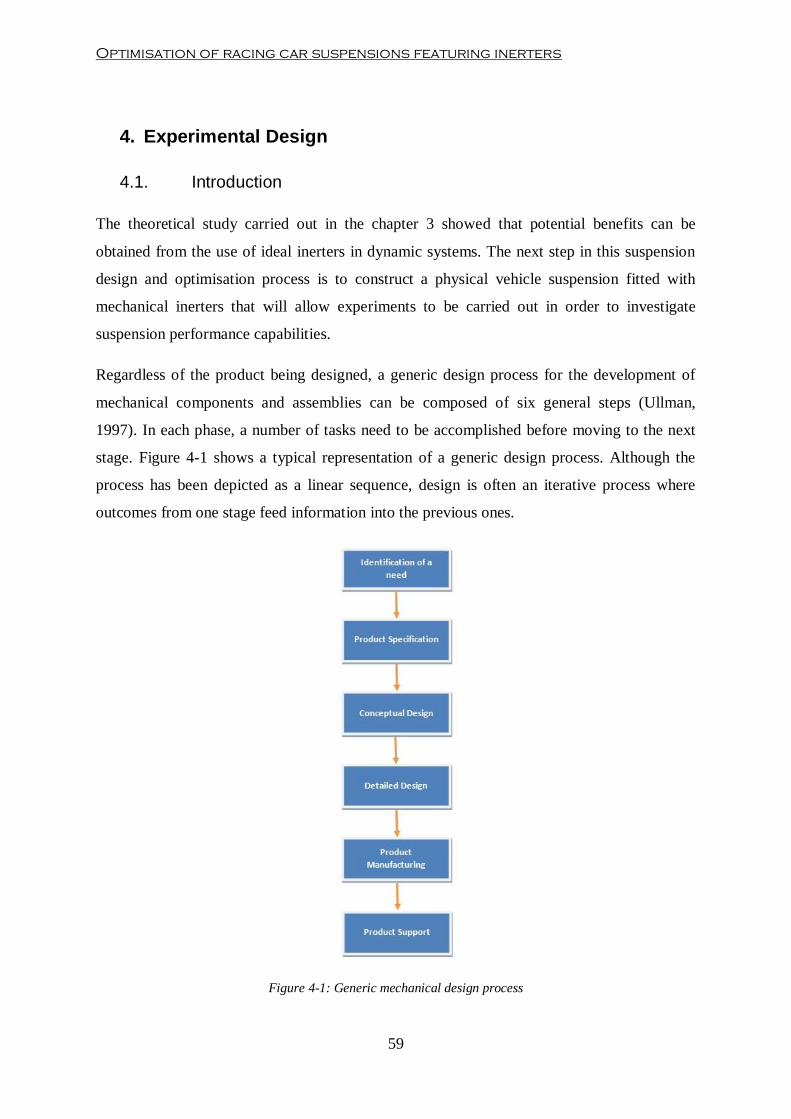
Optimisation of racing car suspensions featuring inerters
59
4. Experimental Design
4.1. Introduction
The theoretical study carried out in the chapter 3 showed that potential benefits can be
obtained from the use of ideal inerters in dynamic systems. The next step in this suspension
design and optimisation process is to construct a physical vehicle suspension fitted with
mechanical inerters that will allow experiments to be carried out in order to investigate
suspension performance capabilities.
Regardless of the product being designed, a generic design process for the development of
mechanical components and assemblies can be composed of six general steps (Ullman,
1997). In each phase, a number of tasks need to be accomplished before moving to the next
stage. Figure 4-1 shows a typical representation of a generic design process. Although the
process has been depicted as a linear sequence, design is often an iterative process where
outcomes from one stage feed information into the previous ones.
Figure 4-1: Generic mechanical design process

Chapter 4- Experimental Design
60
The first part of this chapter has been devoted to the design of the experimental apparatus
according to the mechanical design process depicted in Figure 4-1. The design process
consists of two parts: firstly, design and manufacturing of mechanical inerters; and, secondly,
re-design and modification of a former Formula Student steel space-frame chassis in order to
accommodate the changes to the suspension and layout.
In the second part of the chapter, the experimental test facilities used in the present research
work have been described. The working principle of the Multimatic 4-post rig test facility has
been presented. Furthermore, this chapter describes the rig test instrumentation system and
calibration procedure required to acquire robust, reliable experimental data. The last part of
this chapter has been devoted to describing the method used to analyse raw data obtained
from the data acquisition system and to estimate vehicle suspension experimental parameters.
4.2. Design of Racing Car Suspension incorporating Real Inerters
The design process shown in Figure 4-1 focuses on the design and development of
commercial products. However, most of this process is still valid for the design of research
experimental components. According to this design process, the first stage is the
identification of a need. In this thesis, the design and manufacture of a test car incorporating
real inerters for experimental investigation represents this need. This design consists of two
parts:
Design and manufacture of real inerters
Design and manufacture of a test vehicle capable of accommodating the inerter
alongside the conventional suspension devices.
Due to the nature of the research work, the output of the design process is a prototype chassis
incorporating real inerters. According to this, the last stage in the generic process depicted in
Figure 4-1 does not apply to this thesis.

Optimisation of racing car suspensions featuring inerters
61
4.2.1. Design of a Mechanical Inerter
The process followed to design a physical inerter is summarised in the following figure:
Figure 4-2: Specific design process of a physical inerter
The first stage of this design process is to define a set of engineering specifications, which
will be used as decision criteria in the selection of the most suitable alternative concept. The
following design specifications are critical for the design of a physical inerter:
Design simplicity
Weight
Packaging
Reliability
Maintenance
Adjustability
Interchangeability
Potential parasitic effects
An ideal inerter is defined as “a mechanical one-port device such that the equal and opposite
force applied at the nodes is proportional to the relative acceleration between the nodes”
Smith (2002). In order to generate a force proportional to the acceleration between terminals
several design solutions have been proposed:
Rack-and-pinion-type inerter
Ball-screw-type inerter
Hydraulic-type inerter
In order to select the most suitable design solution, these design alternatives must be
evaluated according to the design criteria identified. The inerter mechanism must be simple.
This simplicity would be translated into fewer mechanical components and a leaner
manufacturing process. The mechanical complexity of ball-screw inerters is low due to the
Product
specifications
Generate
alternatives
Evaluate
alternatives
according to
specifications
Product design
Chapter 4- Experimental Design
62
small amount of mechanical components making up the device. Rack-and-pinion inerters are
more complex than ball-screws inerters because gearing systems need to be designed and
manufactured in order to translate the relative translational motion between inerter’ terminals
into rotational motion of the flywheel. Hydraulic inerters are the most complex option. The
design of hydraulic inerters must include the selection of a proper working fluid, design of
hydraulic lines and valves, and selection of a hydraulic pump and reservoir.
In racing applications, weight and packaging are important design variables in order to
maximise the performance of the vehicle. Due to the amount of components required on a
rack-and-pinion inerter, this option would not be well-suited in terms of packaging and
weight requirements. Hydraulic inerters offer high inertance-to-weight ratios provided a
proper hydraulic circuit design; therefore they are the best option for weight and spatial
savings. Ball-screw inerters present a compromise solution compared to the other two
options. The design is compact but the fact that they need to run flywheels in order to
generate the inertance characteristic (see equation (3.6)) increases its weight.
Although the inerters designed in this research work are prototypes, reliability and
maintenance are important specifications since the devices are meant to be tested under cyclic
dynamic suspension loads. All three options present similar profiles in terms of reliability and
maintenance, with the hydraulic option being the best one. Rack-and-pinion and ballscrew
inerters require periodic lubrication in order to avoid wear and excessive friction.
Another important design factor is adjustability and interchangeability. During a racing
season, GP cars need to race under different track layouts, environmental conditions, etc.
Race car systems must be able to provide a range of adjustability so that maximum
performance can be achieved regardless of these changing conditions. Moreover, components
must be designed so that minimum time is spent during the replacement of components.
Hence, the ability to tune the characteristic property of the device and the possibility of
replacing it efficiently are then desirable. All options offer potentially good adjustability
either by modifying the gear ratio, changing the inertia of the flywheel or redistributing the
flow around a hydraulic pump.
Another aspect to take into consideration is the deviation of a real inerter from its ideal
behaviour. Parasitic effects such as backlash, gear-play, friction, compliance, hydraulic
pressure losses and/or fluid compressibility contribute to this deviation from ideal behaviour.
Rack-and-pinion systems often suffer from gear-play. Tight manufacturing tolerances will

Optimisation of racing car suspensions featuring inerters
63
help to reduce this effect. Ball-screw mechanisms present friction and backlash problems,
although, in this case, backlash can be solved by preloading the balls of the screw.
Furthermore, lubricants create a protective film between two moving parts that allows two
solid surfaces to be separated and therefore friction can be minimised. Finally, hydraulic
inerters have been deemed to produce a large deviation from ideal behaviour (Wang, et al.,
2011).
A decision matrix for the selection of the inerter design solutions has been produced taking
into consideration all the above criteria (see Table 4-1). In this decision matrix, weighting
factors have been set in order to rank the different contribution of design criteria towards the
selection of the final design solution. Moreover, scores have been given to each design
solution according to their individual contribution towards the accomplishment of the criteria.
Criterion Weighting
factor (%)
Physical inerter design solutions
Rack-and-pinion Ball-screw Hydraulic
Raw Weighted Raw Weighted Raw Weighted
Design simplicity 20 50 10 90 18 20 4
Weight 15 20 3 50 7.5 60 9
Packaging 15 10 1.5 70 10.5 90 13.5
Reliability 10 65 6.5 75 7.5 80 8
Maintenance 10 35 3.5 30 3 90 9
Adjustability 15 70 10.5 80 12 90 13.5
Interchangeability 10 40 4 60 6 80 8
Potential parasitic
effects 5 60 3 90 4.5 20 1
TOTAL 100% 42% 69% 66%
Table 4-1: Decision matrix for physical inerter design solutions
According to this decision matrix, the highest overall score corresponds to a ball-screw-type
inerter. Once the appropriate mechanism has been selected, the next step of the design
process is to proceed with the conceptual design (see Figure 4-1). At this stage, the general
basic component layout has been drafted following the designs proposed in Wang et al.
(2009). From this concept design, the main components of the inerter device have been
identified. Moreover, recalling the definition of the working principle of a ball-screw inerter
carried out in Chapter 3, the characteristic inertance b depends on the inertia of the flywheel
Ifw and the lead of the screw l (see equation (3.6)). Hence, adjustments in inertance
Chapter 4- Experimental Design
64
characteristic b can be carried out by adjusting either inertia of the flywheel Ifw or the lead of
the screw l. Since the lead of the screw cannot be modified once it has been manufactured,
the inertia of the flywheel Ifw becomes the only parameter capable of adjusting the inertance
characteristic b.
The next step is then to continue with the detailed mechanical design of the inerter
components. The most complex part in the design of the inerter in terms of manufacturing
complexity is the ball-screw mechanism itself. Furthermore, this component requires
precision machining, special surface shaft treatments and ball preloading. Due to this
manufacturing complexity, the ball-screw mechanism was decided to be purchased from
THK, a manufacturing company specialised in linear guide and ball-screw mechanisms (THK
Co., Ltd., 2012). Therefore, components of the ball-screw mechanism have been designed
following the dimensioning procedure provided by specialist manufacturer THK (THK Co.,
Ltd., 2012). In addition to this, a set of design requirements must be defined in order to
proceed with this dimensioning procedure. In the present research work, three basic
requirements have been identified in order to design a real inerter:
Maximum relative displacement between inerter terminals xstrutD.
Maximum relative velocity between inerter terminals vstrutD.
Maximum relative acceleration between inerter terminals astrutD.
Design values for these requirements have been obtained from Bahrain GP race track profile
data available. In order to select those values, it has been assumed that inputs from race track
are applied directly to the suspension (worst case scenario). According to this, xstrutD has been
obtained from maximum track elevation difference. vstrutD has been calculated from maximum
track elevation gradient assuming a car travelling at vx=90 m/s (324 kph)2. In a similar way,
maximum race track elevation acceleration has been used to obtain astrutD. In addition to this,
a safety factor has been applied to all three design requirements. Table 4-2 shows the design
requirements used to design the ball-screw mechanism.
2 This forward velocity represents standard top speed recorded for current F1 cars Fuente especificada no
válida..
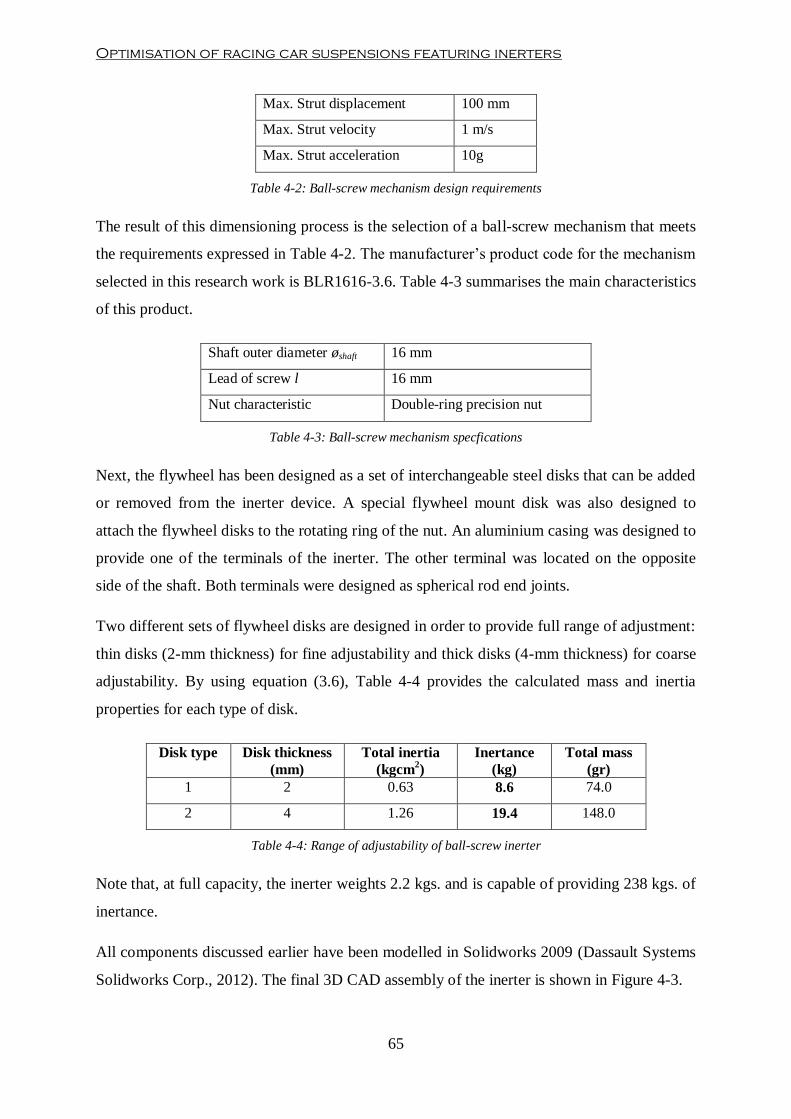
Optimisation of racing car suspensions featuring inerters
65
Max. Strut displacement 100 mm
Max. Strut velocity 1 m/s
Max. Strut acceleration 10g
Table 4-2: Ball-screw mechanism design requirements
The result of this dimensioning process is the selection of a ball-screw mechanism that meets
the requirements expressed in Table 4-2. The manufacturer’s product code for the mechanism
selected in this research work is BLR1616-3.6. Table 4-3 summarises the main characteristics
of this product.
Shaft outer diameter øshaft 16 mm
Lead of screw l 16 mm
Nut characteristic Double-ring precision nut
Table 4-3: Ball-screw mechanism specfications
Next, the flywheel has been designed as a set of interchangeable steel disks that can be added
or removed from the inerter device. A special flywheel mount disk was also designed to
attach the flywheel disks to the rotating ring of the nut. An aluminium casing was designed to
provide one of the terminals of the inerter. The other terminal was located on the opposite
side of the shaft. Both terminals were designed as spherical rod end joints.
Two different sets of flywheel disks are designed in order to provide full range of adjustment:
thin disks (2-mm thickness) for fine adjustability and thick disks (4-mm thickness) for coarse
adjustability. By using equation (3.6), Table 4-4 provides the calculated mass and inertia
properties for each type of disk.
Disk type Disk thickness
(mm)
Total inertia
(kgcm2)
Inertance
(kg)
Total mass
(gr)
1 2 0.63 8.6 74.0
2 4 1.26 19.4 148.0
Table 4-4: Range of adjustability of ball-screw inerter
Note that, at full capacity, the inerter weights 2.2 kgs. and is capable of providing 238 kgs. of
inertance.
All components discussed earlier have been modelled in Solidworks 2009 (Dassault Systems
Solidworks Corp., 2012). The final 3D CAD assembly of the inerter is shown in Figure 4-3.
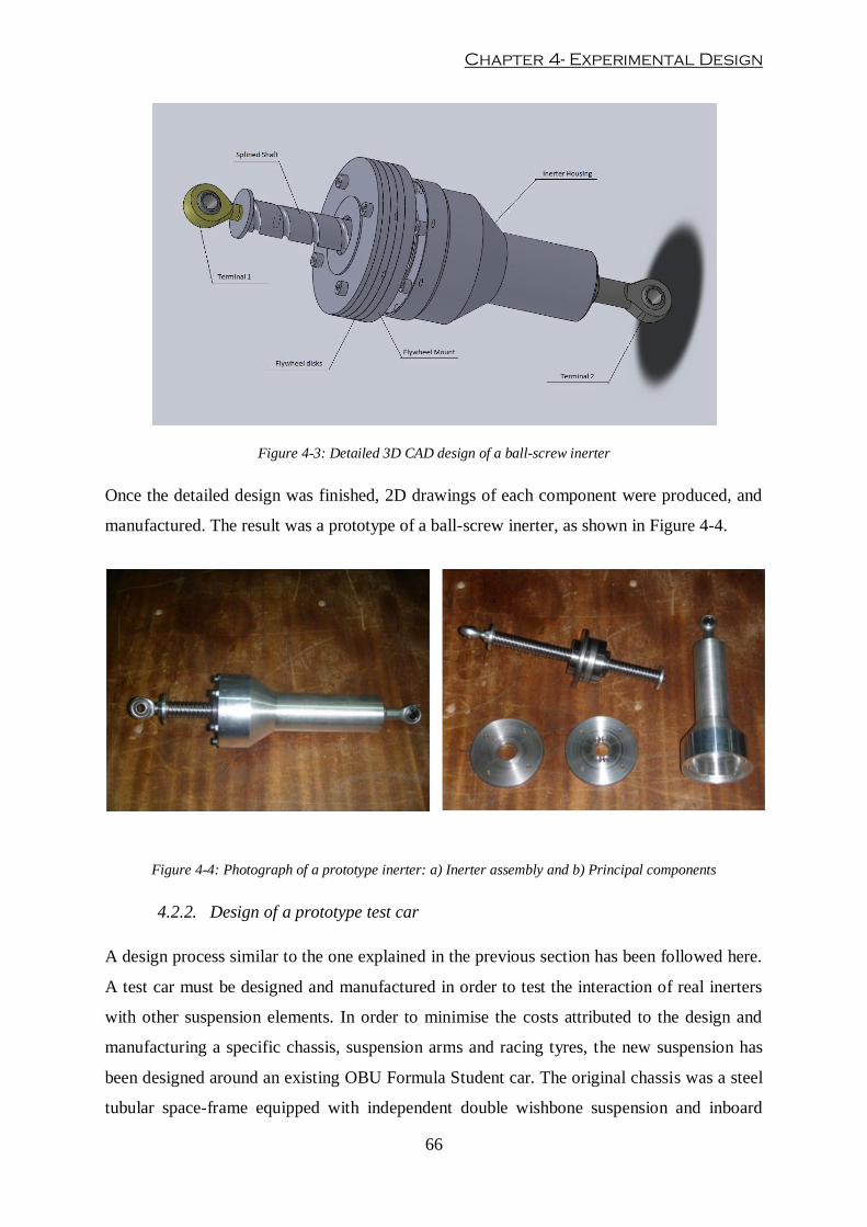
Chapter 4- Experimental Design
66
Figure 4-3: Detailed 3D CAD design of a ball-screw inerter
Once the detailed design was finished, 2D drawings of each component were produced, and
manufactured. The result was a prototype of a ball-screw inerter, as shown in Figure 4-4.
Figure 4-4: Photograph of a prototype inerter: a) Inerter assembly and b) Principal components
4.2.2. Design of a prototype test car
A design process similar to the one explained in the previous section has been followed here.
A test car must be designed and manufactured in order to test the interaction of real inerters
with other suspension elements. In order to minimise the costs attributed to the design and
manufacturing a specific chassis, suspension arms and racing tyres, the new suspension has
been designed around an existing OBU Formula Student car. The original chassis was a steel
tubular space-frame equipped with independent double wishbone suspension and inboard
Optimisation of racing car suspensions featuring inerters
67
spring-dampers at all four corners. The car was also provided with used racing tyres. No
engine, power-train or steering systems were required, since the present thesis focuses on the
analysis of ride dynamics.
The main focus in this section is the re-design of the suspension geometry and layout in order
to accommodate the new components. This re-design includes the definition of all suspension
components excluding suspension arm hard-points as well as the design of new pullrods
(front) and pushrods (rear), rockers, bracket mounting, anti-roll bars (ARBs) and heave
spring-dampers.
The design of the new suspension system can be then split into two areas: kinematic and
dynamic design. In both cases, the major specifications to be taken into consideration in order
to carry out the design process of the new suspension are simplicity, adjustability and
reliability. Suspension components have been designed to be as simple as possible to
facilitate manufacturing and reduce costs. Adjustability is important to allow flexibility in the
study of suspension optimisation. And finally, all components have been designed and
manufactured to endure the loading cycles the test facility will subject them to.
The first step of the detailed design process has been to modify the chassis. Following the
principle of simplicity, only minimal structural modifications of the chassis have been
applied. Cross bars have been added in the cockpit space in order to increase the torsional
stiffness of the chassis. The weight of the driver has been recreated by using sand bags
strapped to the chassis as ballast. The weight of the engine, gearbox and differential has been
replicated by pieces of solid steel attached to the chassis in order to keep the fore/aft balance
of the car as close to 50/50 weight distribution as possible.
The next step in the design process has been to design the kinematics of the suspension. This
includes the definition of a new suspension layout. A new suspension geometry is required in
order to accommodate and package all the suspension components in the space available. The
new suspension layout must account for the following considerations:
Each corner of the car is equipped with an inboard spring-damper unit.
Anti-roll bars are used on both axles. The ARB design consists of a solid torsion bar
connected to each of the rockers via a lever arm and a drop link on each side.

Chapter 4- Experimental Design
68
A 3rd
spring-damper unit can also be added to the suspension in order to control heave
axle excitations at both ends of the car. These devices are connected between rockers.
Front axles are equipped with two inerters connected from the rocker to the chassis;
meanwhile the rear axle is equipped with one axle inerter connected between rockers
According to this, both front and rear rockers have been completely re-designed in order to
accommodate all the new components mentioned previously. Rear rockers have also been
placed in a new location with respect to the previous design for better packaging.
Furthermore, following the principle of adjustability, rockers have been designed so that
different suspension characteristics can be obtained. All rockers present 3 different pull-
rod/push-rod joint points, so that, by changing this position, different motion ratios can be
induced, therefore modifying the spring and damper rates experienced at the tyre contact
patch. Since no steering system was provided, steering links have been welded to the front
wishbones in order to avoid undesired tyre steering vibrations.
3D kinematic models of front and rear suspensions have been created in the multibody
dynamics (MBD) software MSC.Adams R3 (MSC Software, 2012). Figure 4-5 and Figure
4-6 show the layout of the new front and rear suspension respectively. Components have
been colour-coded to facilitate their identification within the model (see Table 4-5).
Figure 4-5: 3D MBD kinematic model of re-designed front suspension

Optimisation of racing car suspensions featuring inerters
69
Figure 4-6: 3D MBD kinematic model of re-designed rear suspension
Colour Suspension Component
Silver Wheel and tyre assembly
Red Suspension arms and upright
Yellow Pull-rod (front) and push-rod (rear)
Magenta Rocker
Blue Corner spring-damper unit
Green Inerter
Orange Axle spring-damper unit
White ARB drop link and lever arm
Table 4-5: Colour-coded key table for MBD suspension models
The main purpose of these models was to evaluate the packaging and the kinematic
movement of the suspension. Accordingly, these kinematic MBD models have been used to
define the suspension layout and the location of the attachment positions of the new
suspension components to the rocker, on one end, and to the chassis, on the other end. These
hard points have been designed to provide a near constant installation ratio (IR) between
wheel vertical travel and suspension components along the suspension movement range due
Chapter 4- Experimental Design
70
to the fact that it will facilitate future suspension modelling and analysis since the IR can be
considered a constant value.
Once the kinematic model was finished, a 3D CAD model of the re-designed vehicle was
produced. All components were designed and assembled into the chassis in Solidworks 2009
(Dassault Systems Solidworks Corp., 2012).
The final stage of the design process was devoted to the design of the suspension from a
dynamic point of view. In this phase, spring stiffnesses of elastic components and damping
rates have been defined. The main specification has been adjustability. The suspension has
been designed so that it was possible to achieve a stiffness range from a relative softly sprung
car (ride frequency of about 1.5 Hz) up to a heavily sprung car (ride frequency over 6 Hz).
These limits would correspond to suspensions for production sports cars for the lower bound
of the ride frequency range and to suspensions for high performance competition cars with
aerodynamic effects, such as Formula 1 cars, for the upper bound. Table 4-6 shows a
summary of the design spring stiffness required to achieve a particular suspension ride
frequency for one of the rear corners.
Four sets of springs have been selected: 100 (17.5), 200 (35), 350 (61.3) and 500 (87.6) lb/in
(N/mm)3. This range covers a ride frequency from 1.5 to 4 Hz (see Table 4-6). Ride
frequency could be further increased by adding a 3rd
spring to the axle. A similar table could
be produced in order to select the appropriate ride frequency for the axle spring. Two sets of
axle springs were selected: 900 (157.6) and 1100 (192.6) lb/in (N/mm).
3 Spring manufacturers typically provide spring stiffness specifications in imperial units
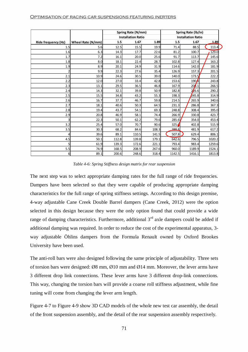
Optimisation of racing car suspensions featuring inerters
71
Table 4-6: Spring Stiffness design matrix for rear suspension
The next step was to select appropriate damping rates for the full range of ride frequencies.
Dampers have been selected so that they were capable of producing appropriate damping
characteristics for the full range of spring stiffness settings. According to this design premise,
4-way adjustable Cane Creek Double Barrel dampers (Cane Creek, 2012) were the option
selected in this design because they were the only option found that could provide a wide
range of damping characteristics. Furthermore, additional 3rd
axle dampers could be added if
additional damping was required. In order to reduce the cost of the experimental apparatus, 3-
way adjustable Öhlins dampers from the Formula Renault owned by Oxford Brookes
University have been used.
The anti-roll bars were also designed following the same principle of adjustability. Three sets
of torsion bars were designed: Ø8 mm, Ø10 mm and Ø14 mm. Moreover, the lever arms have
3 different drop link connections. These lever arms have 3 different drop-link connections.
This way, changing the torsion bars will provide a coarse roll stiffness adjustment, while fine
tuning will come from changing the lever arm length.
Figure 4-7 to Figure 4-9 show 3D CAD models of the whole new test car assembly, the detail
of the front suspension assembly, and the detail of the rear suspension assembly respectively.
1.5 1.67 1.89 1.5 1.67 1.89
1.5 5.6 12.5 15.5 19.9 71.4 88.5 113.4
1.6 6.3 14.3 17.7 22.6 81.2 100.7 129.0
1.7 7.2 16.1 20.0 25.6 91.7 113.7 145.6
1.8 8.0 18.1 22.4 28.7 102.8 127.4 163.2
1.9 8.9 20.1 24.9 31.9 114.6 142.0 181.9
2 9.9 22.3 27.6 35.4 126.9 157.3 201.5
2.1 10.9 24.6 30.5 39.0 140.0 173.5 222.2
2.2 12.0 27.0 33.4 42.8 153.6 190.4 243.8
2.3 13.1 29.5 36.5 46.8 167.9 208.1 266.5
2.4 14.3 32.1 39.8 50.9 182.8 226.6 290.2
2.5 15.5 34.8 43.2 55.3 198.3 245.8 314.9
2.6 16.7 37.7 46.7 59.8 214.5 265.9 340.6
2.7 18.1 40.6 50.3 64.5 231.3 286.8 367.3
2.8 19.4 43.7 54.1 69.3 248.8 308.4 395.0
2.9 20.8 46.9 58.1 74.4 266.9 330.8 423.7
3 22.3 50.1 62.2 79.6 285.6 354.0 453.4
3.2 25.4 57.0 70.7 90.6 325.0 402.8 515.9
3.5 30.3 68.2 84.6 108.3 388.8 481.9 617.2
4 39.6 89.1 110.5 141.5 507.8 629.4 806.1
4.5 50.1 112.8 139.8 179.1 642.6 796.5 1020.2
5 61.9 139.3 172.6 221.1 793.4 983.4 1259.6
5.5 74.9 168.5 208.9 267.6 960.0 1189.9 1524.1
6 89.1 200.6 248.6 318.4 1142.5 1416.1 1813.8
Wheel Rate (N/mm)
Spring Rate (N/mm) Spring Rate (lb/in)
Installation Ratio Installation Ratio
Ride frequency (Hz)
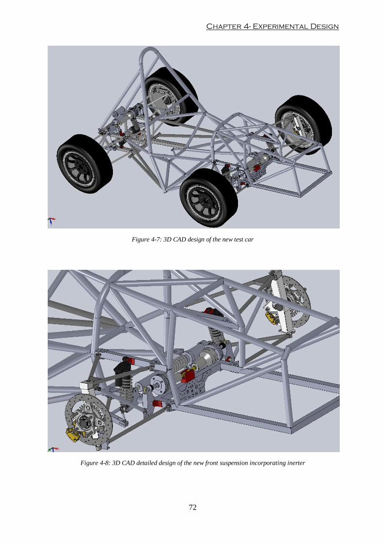
Chapter 4- Experimental Design
72
Figure 4-7: 3D CAD design of the new test car
Figure 4-8: 3D CAD detailed design of the new front suspension incorporating inerter

Optimisation of racing car suspensions featuring inerters
73
Figure 4-9: 3D CAD detailed design of the new rear suspension incorporating inerter
Finally, 2D CAD drawings for suspension components and assemblies were produced from
the previous 3D models and manufactured in the OBU workshop. The final result is a
reconditioned test car with inerters as shown in Figure 4-10 to Figure 4-12.
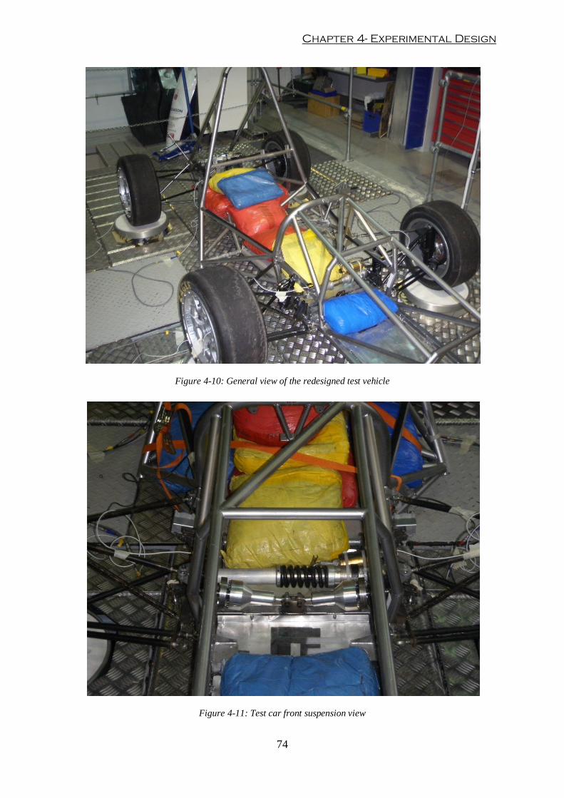
Chapter 4- Experimental Design
74
Figure 4-10: General view of the redesigned test vehicle
Figure 4-11: Test car front suspension view

Optimisation of racing car suspensions featuring inerters
75
Figure 4-12: Test car rear suspension view
4.3. Experimental Test System Description
The experimental test facility used in this research work was the Multimatic four-post rig
facility at Oxford Brookes University. This facility has been custom designed and installed by
Multimatic Technical Centre Europe (Multimatic Technical Centre, 2011). Figure 4-13 and
Figure 4-14 show the four-post rig test facility.

Chapter 4- Experimental Design
76
Figure 4-13: Upper view of OBU Four-post rig test facility
Figure 4-14: Lower view of OBU Four-post rig test facility
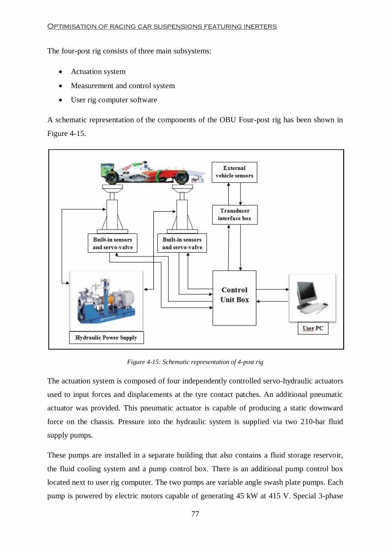
Optimisation of racing car suspensions featuring inerters
77
The four-post rig consists of three main subsystems:
Actuation system
Measurement and control system
User rig computer software
A schematic representation of the components of the OBU Four-post rig has been shown in
Figure 4-15.
Figure 4-15: Schematic representation of 4-post rig
The actuation system is composed of four independently controlled servo-hydraulic actuators
used to input forces and displacements at the tyre contact patches. An additional pneumatic
actuator was provided. This pneumatic actuator is capable of producing a static downward
force on the chassis. Pressure into the hydraulic system is supplied via two 210-bar fluid
supply pumps.
These pumps are installed in a separate building that also contains a fluid storage reservoir,
the fluid cooling system and a pump control box. There is an additional pump control box
located next to user rig computer. The two pumps are variable angle swash plate pumps. Each
pump is powered by electric motors capable of generating 45 kW at 415 V. Special 3-phase
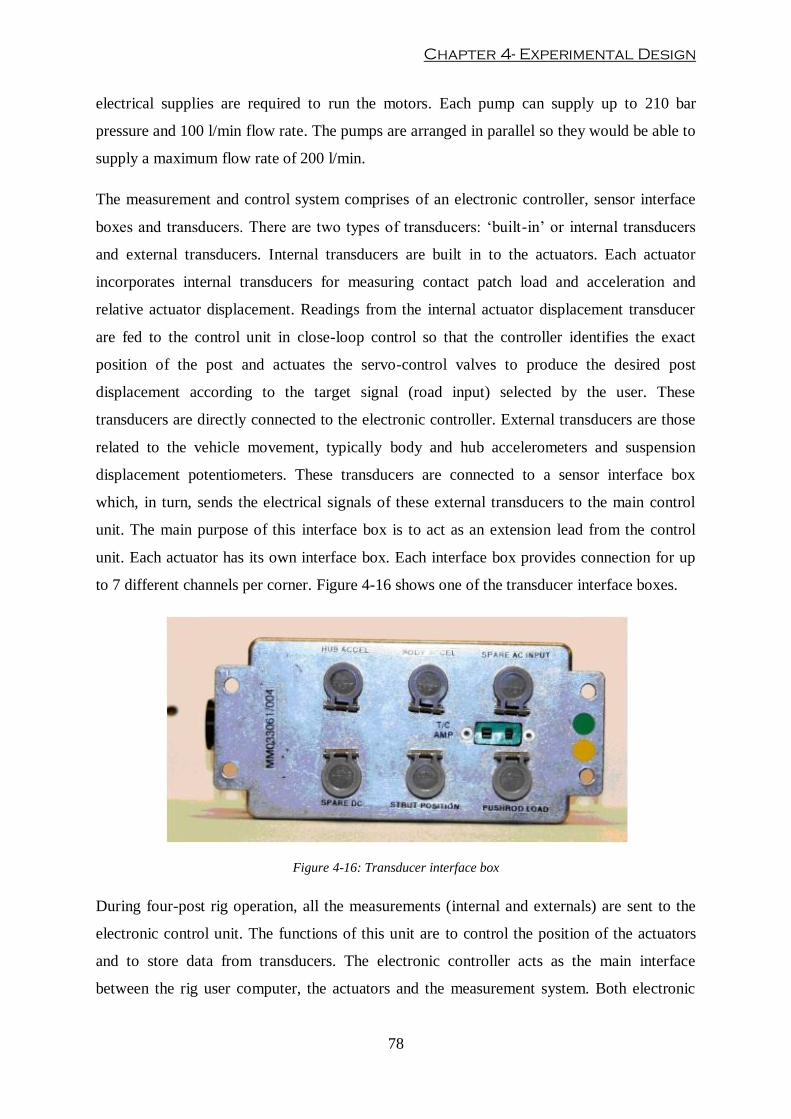
Chapter 4- Experimental Design
78
electrical supplies are required to run the motors. Each pump can supply up to 210 bar
pressure and 100 l/min flow rate. The pumps are arranged in parallel so they would be able to
supply a maximum flow rate of 200 l/min.
The measurement and control system comprises of an electronic controller, sensor interface
boxes and transducers. There are two types of transducers: ‘built-in’ or internal transducers
and external transducers. Internal transducers are built in to the actuators. Each actuator
incorporates internal transducers for measuring contact patch load and acceleration and
relative actuator displacement. Readings from the internal actuator displacement transducer
are fed to the control unit in close-loop control so that the controller identifies the exact
position of the post and actuates the servo-control valves to produce the desired post
displacement according to the target signal (road input) selected by the user. These
transducers are directly connected to the electronic controller. External transducers are those
related to the vehicle movement, typically body and hub accelerometers and suspension
displacement potentiometers. These transducers are connected to a sensor interface box
which, in turn, sends the electrical signals of these external transducers to the main control
unit. The main purpose of this interface box is to act as an extension lead from the control
unit. Each actuator has its own interface box. Each interface box provides connection for up
to 7 different channels per corner. Figure 4-16 shows one of the transducer interface boxes.
Figure 4-16: Transducer interface box
During four-post rig operation, all the measurements (internal and externals) are sent to the
electronic control unit. The functions of this unit are to control the position of the actuators
and to store data from transducers. The electronic controller acts as the main interface
between the rig user computer, the actuators and the measurement system. Both electronic

Optimisation of racing car suspensions featuring inerters
79
control unit and the actuation system are expensive pieces of equipment. By decoupling the
host computer from the control and actuation systems, these systems can be protected from
potential external risks associated to the user PC such as viruses or software corruption which
could ultimately damage the testing equipment.
The last component of the test rig is the user software. This software is called Dynosoft MX
and it is used to operate and display test data. This software is connected via a USB link to
the control unit. A view of the command window is shown in Figure 4-17.
Figure 4-17: Four-post rig main command window
The main features of the software are:
Calibration of measurement channels
Definition and control of input waveforms, sampling rates, vibration modes
Data acquisition, storage and export of all transducers measurements
Display of data as a function of time and ‘XY’ plots
Calculation of math channels and simple data processing operations

Chapter 4- Experimental Design
80
For detailed specifications, operational and a more in-depth description of the working
principle of the rig, the reader is referred to the Multimatic Four Post Technical Specification
and Operating Manual (Multimatic Technical Centre, 2011).
4.4. System calibration Procedure
Initial calibration of the Four-post Rig was carried out when the rig was commissioned in
August 2008. This calibration was carried out by the Multimatic technicians and a certificate
of calibration was presented. Furthermore, certified annual calibrations have been carried out
during each annual service by Multimatic. The last service dates from October 2011. A copy
of the certificate has been included in Appendix A. This process includes the calibration of
the actuator load cells, accelerometer and displacement potentiometer as well as the
calibration of the body and hub accelerometers and strut displacement string potentiometers.
In addition to this annual calibration, strut displacement string potentiometers and body and
hub accelerometers calibration settings are checked regularly in order to ensure that the
output data is fully reliable. Dynosoft MX software allows calibration settings monitoring
and manipulation.
For suspension displacement potentiometers, the calibration check is carried out by
measuring the displacement of the sensor with a vernier calliper and recording the voltage
measured by the software. This process is repeated for two different displacements and
calibration is obtained as the gradient of displacement to voltage. An additional intermediate
displacement is used to check that the sensor has been properly calibrated.
In the case of accelerometers, the calibration check is done both dynamically and statically.
Dynamically, body and hub accelerometers of each corner are fixed to their respective
actuator with the PTFE pads removed. A sinusoidal input wave is applied. Measured
acceleration values are then compared against the actuator pad acceleration in a XY plot. If
the difference in the accelerometer outputs is more than 1% RMS then the hub and/or body
accelerometer calibration settings are modified to match the slopes. This process does not
offer an absolute calibration of the system; as this method is conditioned by pad acceleration.
If the pad acceleration was incorrect, then the rest of calibration would be incorrect as well.
In order to overcome this limitation, an additional static accelerometer calibration is also
carried out. Body and hub accelerometers are placed on a flat surface in upright posit ion. A
calibrated accelerometer should read 1g of vertical acceleration (gravity action).

Optimisation of racing car suspensions featuring inerters
81
Accelerometers are then turned upside down and they should read -1g. If a deviation of more
than 1% from these values occurs, a scaling factor is applied to the gradient of acceleration
over voltage.
An additional benefit of a combined static and dynamic method for accelerometer calibration
is that it could detect potential errors of calibration in the pad accelerometers.
4.5. Parameter Determination Method
The main aims of a four-post rig can be described as:
Estimation of suspension and vehicle parameters
Optimisation of suspension performance
General chassis diagnostics
In this section, special attention has been paid to the first of these objectives. Acquired
parameters from experimental testing present a series of benefits: they can be used to
compare experimental measurements against design variables and identify potential
improvements in design (iterative design process); they can also be used to develop vehicle
models in simulation. If properly validated, these models can accurately represent the real
behaviour of the vehicle and could then be used to run off-line computer suspension
optimisation. One of the main benefits of this process is that it produces important savings in
cost, because fewer components need to be manufactured at the prototyping stage, and time
for optimisation is reduced, as optimisation algorithms are capable of sweeping through
hundreds of suspension set-ups in a reduced amount of time.
In this section, the operating process of the rig has been explained. Furthermore, the method
for parameter estimation developed by a research student in the Department of Mechanical
Engineering at Oxford Brookes University has been briefly described (Bennett, 2012). This
method has been then extended so that parameters related to real inerters and nonlinear tyres
can be also determined.
4.5.1. Set of parameters required
A four-post rig recreates road inputs experienced by a vehicle whilst driving on a road and/or
race track. These road inputs can be typically decomposed into 4 independent vibration
modes:

Chapter 4- Experimental Design
82
Heave mode: all 4 wheel are in phase
Pitch mode: front and rear wheels out of phase by 180º
Roll mode: left and right wheels out of phase by 180º
Warp or articulation mode: cross diagonal wheels out of phase by 180º
According to this, in order to simulate the response of a vehicle to all these vibration modes
on a test rig, the simplest model that could be used is a simplified 7-DOF system (see Figure
4-18).
Figure 4-18: Simplified 7-DOF vehicle suspension model (Bennett, 2012)
The set of vehicle parameters required for simulating a validated model that can be estimated
from experimental testing include overall vehicle dimensions, mass properties for all bodies
(sprung and unsprung masses), suspension characteristics and tyre parameters.
Overall vehicle dimensions such as wheelbase wb, front track tf and rear track tr can be
directly measured. All four corner weights WFL, WFR, WRL and WRR can be measured from the
actuator load cells when the car is standing still (no dynamic inputs applied). The overall
mass of the vehicle WTot can then be obtained by adding all four corner weights (see eq.
(4.1)).
Furthermore, longitudinal weight distribution Long_WDist, lateral weight distribution
Lat_WDist, diagonal weight distribution Diag_WDist and distances from CoG to front axle a
and to rear axle b can also be calculated from corner weights using equations (4.2) to (4.6).

Optimisation of racing car suspensions featuring inerters
83
Note that, distances a and b have been obtained from the overall longitudinal weight
distribution of the vehicle. Once front and rear unsprung masses have been estimated,
longitudinal sprung weight distribution Long_WDist_Sprung could be obtained and a and b
re-calculated.
Unsprung masses, chassis inertias and suspension and tyre characteristics will require the use
of dynamic inputs in order to be estimated.
4.5.2. Vehicle Instrumentation Procedure
The vehicle is instrumented with 12 external transducers arranged as follows:
4 Body accelerometers (1 per corner)
4 Hub accelerometers (1 per corner)
4 Strut displacement potentiometers (1 per corner)
Accelerometers are attached to the components using a thin layer of ‘blu-tac’. In this way, the
accelerometers can be easily removed and replaced at any other location. ‘Blu-tac’ also
provides a flexible mounting that allows the sensors to be placed in non-horizontal surfaces.
Accelerometers are aligned to the gravity field using a spirit level. In addition to this, ‘blu-
tac’ acts as a natural high-pass filter. It filters out very high frequency contents (>50 Hz)
associated with noise.
Body accelerometers have been fitted to each of the corners of the chassis. The ideal location
of the accelerometers is in a stiff part of the chassis as close as possible to the vertical axis
directly above the wheel centre. In this way the measurements are taken at the same points as

Chapter 4- Experimental Design
84
where accelerations are modelled in a lumped-mass dynamic vehicle model. However, due to
the space-frame chassis construction, accelerometers cannot be placed exactly in this
position. Instead, they are placed as close as possible to the axle centreline and as far away as
possible from each other. Relative positions of all the accelerometers with respect to the
wheels have then been measured. Figure 4-19 and Figure 4-20 show the location of the body
accelerometers at all the corners.
Figure 4-19: Front body accelerometer location
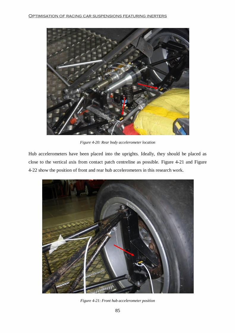
Optimisation of racing car suspensions featuring inerters
85
Figure 4-20: Rear body accelerometer location
Hub accelerometers have been placed into the uprights. Ideally, they should be placed as
close to the vertical axis from contact patch centreline as possible. Figure 4-21 and Figure
4-22 show the position of front and rear hub accelerometers in this research work.
Figure 4-21: Front hub accelerometer position
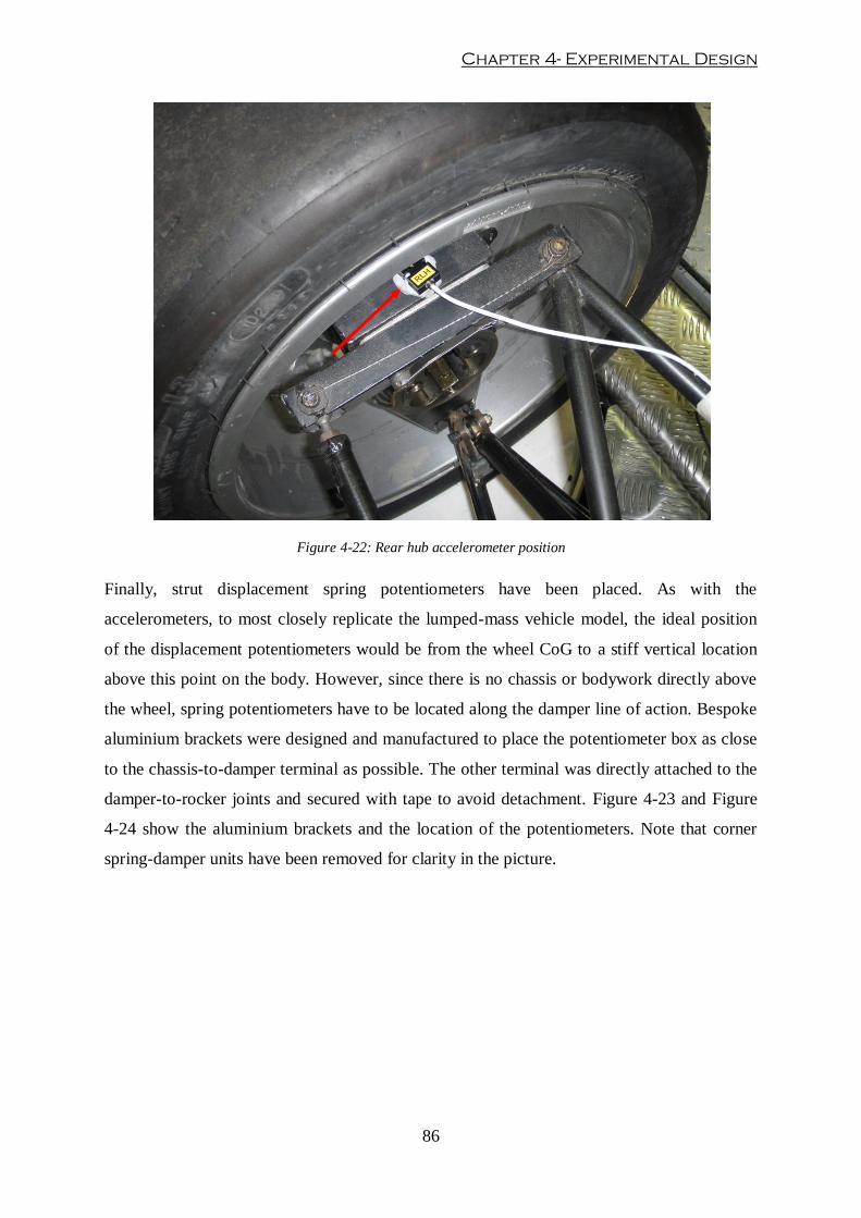
Chapter 4- Experimental Design
86
Figure 4-22: Rear hub accelerometer position
Finally, strut displacement spring potentiometers have been placed. As with the
accelerometers, to most closely replicate the lumped-mass vehicle model, the ideal position
of the displacement potentiometers would be from the wheel CoG to a stiff vertical location
above this point on the body. However, since there is no chassis or bodywork directly above
the wheel, spring potentiometers have to be located along the damper line of action. Bespoke
aluminium brackets were designed and manufactured to place the potentiometer box as close
to the chassis-to-damper terminal as possible. The other terminal was directly attached to the
damper-to-rocker joints and secured with tape to avoid detachment. Figure 4-23 and Figure
4-24 show the aluminium brackets and the location of the potentiometers. Note that corner
spring-damper units have been removed for clarity in the picture.

Optimisation of racing car suspensions featuring inerters
87
Figure 4-23: Front strut displacement potentiometer position
Figure 4-24: Rear strut displacement potentiometer location

Chapter 4- Experimental Design
88
4.5.3. Four-Post Rig Operation Procedure
Once the car was instrumented, the tyre pressures had to be properly set to normal race
conditions. The tyre pressures modify the vertical tyre characteristics and therefore have an
important impact on the dynamic response of the car. Pressures may change slightly during a
test session, so they are frequently reset. Tyre pressures can also be changed to study the
behaviour of the suspension from the beginning of the race (low pressure) to the end of the
race (high pressure).
With tyre pressures properly set, corner weights are measured and reset if necessary. First,
corner weights are checked accounting only for the car. After that, fuel is added and the
driver enters the cockpit and new measurements are taken. If the weight distribution does not
coincide with normal race conditions, modifications to the suspension static settings are made
to regain the desired weight distribution. Due to Health & Safety policies at Oxford Brookes
University, a physical person is not allowed to be inside a racing test car at any time during
rig testing. According to this policy, the driver is substituted by ballast. Sand bags are used to
replicate the weight of driver. Colour coded sand bags have been used to simulate the weight
of different human body areas:
Red coloured sand bag (18 kg): Two sand bags have been used to simulate human
torso.
Yellow coloured sand bag (15 kg): Used to simulate the weight of the legs. One or
two yellow sand bags would normally be used depending on driver’s weight.
Blue coloured sand bag (10 kg): Used to simulate upper body and head and driver’s
feet.
In addition to this, if fuel is not available, sand bags could also be used to simulate the weight
of fuel load. Sand bags can then be placed into the driver’s cockpit until desired overall
weight and weight distribution are reached. Figure 4-25 shows an example of weight setting.
Figure 4-25: Four-post rig weight setting procedure
Corner Weights FL FR RL RR Total % Front % Cross % Left
Car Only 97,7 95,7 168 173 534,4 36,19 50,65 49,72
Car + Driver +15 kg 122 123 179 200 624 39,26 51,60 48,24
Car + Ballast 123 121 176 200 620 39,35 52,10 48,23

Optimisation of racing car suspensions featuring inerters
89
If suspension displacement transducers are not positioned directly above the wheel centreline
to a vertical position above it in the chassis, as is the case in most racing cars, an installation
ratio (IR) must be measured. In this case, the installation ratio represents the wheel movement
relative to the suspension potentiometer movement. In order to obtain the installat ion ratio,
the springs and dampers must be disconnected from the suspension and the car has to be
placed onto axle stands. The actuator height is set so that the wheels are in race track ride
height conditions. With the wheels free to move relative to the chassis, a nonlinear low
frequency sine wave (see Figure 4-26) is then applied. Using the Dynosoft MX software, an
‘XY’ graph is plotted to obtain the installation ratio. In this graph, the actuator displacement
(y-axis) has been plotted against suspension displacement (x-axis) for each corner. The
gradient of this plot represents the installation ratio (See Figure 4-27).
Figure 4-26: Installation ratio test input wave
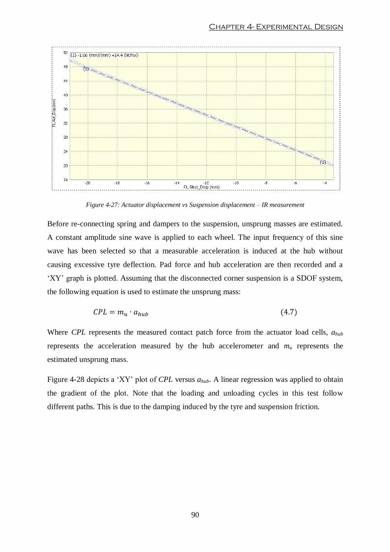
Chapter 4- Experimental Design
90
Figure 4-27: Actuator displacement vs Suspension displacement – IR measurement
Before re-connecting spring and dampers to the suspension, unsprung masses are estimated.
A constant amplitude sine wave is applied to each wheel. The input frequency of this sine
wave has been selected so that a measurable acceleration is induced at the hub without
causing excessive tyre deflection. Pad force and hub acceleration are then recorded and a
‘XY’ graph is plotted. Assuming that the disconnected corner suspension is a SDOF system,
the following equation is used to estimate the unsprung mass:
Where CPL represents the measured contact patch force from the actuator load cells, ahub
represents the acceleration measured by the hub accelerometer and mu represents the
estimated unsprung mass.
Figure 4-28 depicts a ‘XY’ plot of CPL versus ahub. A linear regression was applied to obtain
the gradient of the plot. Note that the loading and unloading cycles in this test follow
different paths. This is due to the damping induced by the tyre and suspension friction.
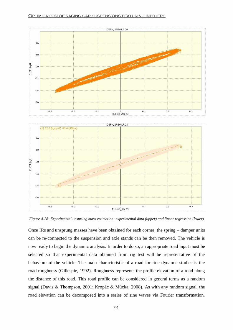
Optimisation of racing car suspensions featuring inerters
91
Figure 4-28: Experimental unsprung mass estimation: experimental data (upper) and linear regression (lower)
Once IRs and unsprung masses have been obtained for each corner, the spring – damper units
can be re-connected to the suspension and axle stands can be then removed. The vehicle is
now ready to begin the dynamic analysis. In order to do so, an appropriate road input must be
selected so that experimental data obtained from rig test will be representative of the
behaviour of the vehicle. The main characteristic of a road for ride dynamic studies is the
road roughness (Gillespie, 1992). Roughness represents the profile elevation of a road along
the distance of this road. This road profile can be considered in general terms as a random
signal (Davis & Thompson, 2001; Kropác & Múcka, 2008). As with any random signal, the
road elevation can be decomposed into a series of sine waves via Fourier transformation.
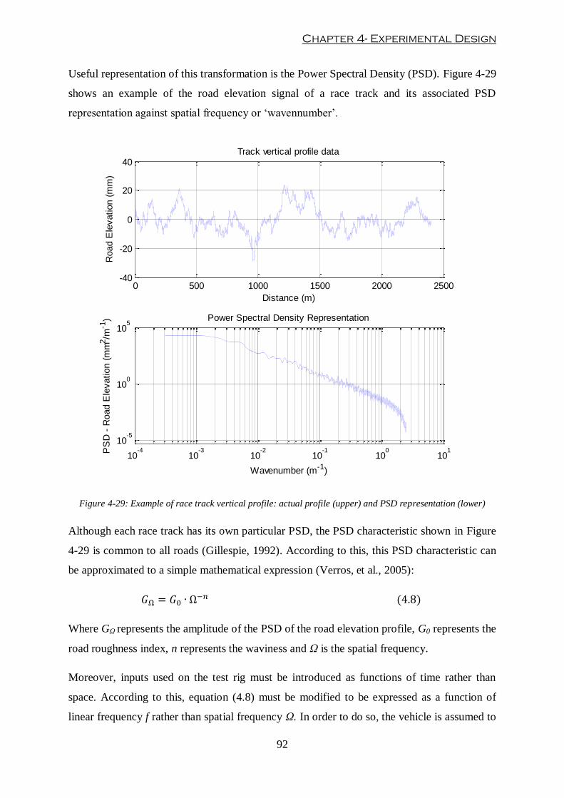
Chapter 4- Experimental Design
92
Useful representation of this transformation is the Power Spectral Density (PSD). Figure 4-29
shows an example of the road elevation signal of a race track and its associated PSD
representation against spatial frequency or ‘wavennumber’.
Figure 4-29: Example of race track vertical profile: actual profile (upper) and PSD representation (lower)
Although each race track has its own particular PSD, the PSD characteristic shown in Figure
4-29 is common to all roads (Gillespie, 1992). According to this, this PSD characteristic can
be approximated to a simple mathematical expression (Verros, et al., 2005):
Where GΩ represents the amplitude of the PSD of the road elevation profile, G0 represents the
road roughness index, n represents the waviness and Ω is the spatial frequency.
Moreover, inputs used on the test rig must be introduced as functions of time rather than
space. According to this, equation (4.8) must be modified to be expressed as a function of
linear frequency f rather than spatial frequency Ω. In order to do so, the vehicle is assumed to
0 500 1000 1500 2000 2500-40
-20
0
20
40Track vertical profile data
Distance (m)
Road E
levation (
mm
)
10-4
10-3
10-2
10-1
100
101
10-5
100
105
Wavenumber (m-1)
PS
D -
Road E
levation (
mm
2/m
-1) Power Spectral Density Representation
Optimisation of racing car suspensions featuring inerters
93
travel at constant forward velocity Vx. Therefore, linear and spatial frequencies can be related
as follows:
And so, equation (4.8) can be re-arranged as follows:
Where Gf represents the amplitude of the PSD of the road elevation profile with respect to
linear frequency f and Gf0 can be expressed as:
Equation (4.10) can then be represented as a straight line in a log-log plot and parameters Gf0
and n can be estimated by linear regression. Equation (4.11) highlights that both road
roughness index and vehicle forward speed produce the same impact in the generation of road
input excitations, i.e. an increase in PSD amplitudes can represent either a vehicle travelling
at the same speed on a rougher road or a vehicle travelling along the same road at higher
speed. Figure 4-30 shows an example of experimental PSD and the linear approximation
achieved with equation (4.10).
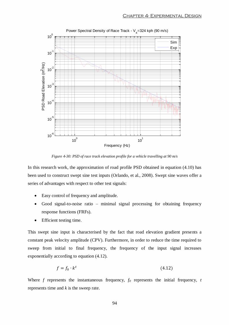
Chapter 4- Experimental Design
94
Figure 4-30: PSD of race track elevation profile for a vehicle travelling at 90 m/s
In this research work, the approximation of road profile PSD obtained in equation (4.10) has
been used to construct swept sine test inputs (Orlando, et al., 2008). Swept sine waves offer a
series of advantages with respect to other test signals:
Easy control of frequency and amplitude.
Good signal-to-noise ratio – minimal signal processing for obtaining frequency
response functions (FRFs).
Efficient testing time.
This swept sine input is characterised by the fact that road elevation gradient presents a
constant peak velocity amplitude (CPV). Furthermore, in order to reduce the time required to
sweep from initial to final frequency, the frequency of the input signal increases
exponentially according to equation (4.12).
Where f represents the instantaneous frequency, f0 represents the initial frequency, t
represents time and k is the sweep rate.
100
101
10-6
10-5
10-4
10-3
10-2
10-1
100
Frequency (Hz)
PS
D R
oad E
levation (
m2/H
z)
Power Spectral Density of Race Track - Vx=324 kph (90 m/s)
Sim
Exp
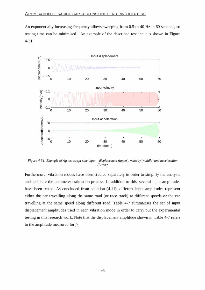
Optimisation of racing car suspensions featuring inerters
95
An exponentially increasing frequency allows sweeping from 0.5 to 40 Hz in 60 seconds, so
testing time can be minimised. An example of the described test input is shown in Figure
4-31.
Figure 4-31: Example of rig test swept sine input – displacement (upper), velocity (middle) and acceleration
(lower)
Furthermore, vibration modes have been studied separately in order to simplify the analysis
and facilitate the parameter estimation process. In addition to this, several input amplitudes
have been tested. As concluded from equation (4.11), different input amplitudes represent
either the car travelling along the same road (or race track) at different speeds or the car
travelling at the same speed along different road. Table 4-7 summarises the set of input
displacement amplitudes used in each vibration mode in order to carry out the experimental
testing in this research work. Note that the displacement amplitude shown in Table 4-7 refers
to the amplitude measured for f0.
0 10 20 30 40 50 60-0.05
0
0.05Input displacement
Dis
pla
cem
ent(
m)
0 10 20 30 40 50 60-0.1
0
0.1Input velocity
Velo
city(m
/s)
0 10 20 30 40 50 60-20
0
20Input acceleration
time(secs)
Accele
ration(m
/s2)

Chapter 4- Experimental Design
96
Mode Amplitude (mm)
Heave
20
25
30
35
Pitch 20
25
Roll
30
20
25
Warp 4
8
Table 4-7: Summary of test inputs used in experimental testing
After tests have been carried out, time-domain data from sensors is obtained. Dynosoft MX
software presents limited processing and analysis capabilities, so data is exported as ‘.txt’
files to allow for more complex analysis in in-house built software. The following section
briefly describes the operating principle of this post-processing tool.
4.5.4. Frequency Analysis and Parameter Estimation Software
Because of the limited analysis capabilities of Dynosoft MX, new software had to be
developed in order to estimate vehicle suspension parameters and to conduct frequency-
domain analysis of the experimental data. This software was designed and developed by
Bennet (2012). Detailed explanation of data filtering processes, complex analysis and
parameter estimation algorithm can be found in his work (Bennett, 2012). The main functions
of this software are to obtain the frequency response functions (FRFs) of measured dynamic
magnitudes; to support advanced suspension and vehicle dynamics analysis; and to estimate
the required parameters for accurate vehicle simulation.
The software was written as a Graphical User Interface (GUI) in Matlab. Figure 4-32 depicts
the main command window of the program.
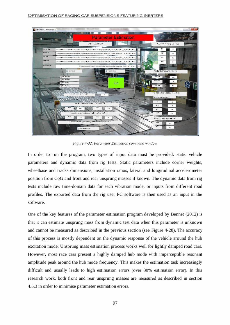
Optimisation of racing car suspensions featuring inerters
97
Figure 4-32: Parameter Estimation command window
In order to run the program, two types of input data must be provided: static vehicle
parameters and dynamic data from rig tests. Static parameters include corner weights,
wheelbase and tracks dimensions, installation ratios, lateral and longitudinal accelerometer
position from CoG and front and rear unsprung masses if known. The dynamic data from rig
tests include raw time-domain data for each vibration mode, or inputs from different road
profiles. The exported data from the rig user PC software is then used as an input in the
software.
One of the key features of the parameter estimation program developed by Bennet (2012) is
that it can estimate unsprung mass from dynamic test data when this parameter is unknown
and cannot be measured as described in the previous section (see Figure 4-28). The accuracy
of this process is mostly dependent on the dynamic response of the vehicle around the hub
excitation mode. Unsprung mass estimation process works well for lightly damped road cars.
However, most race cars present a highly damped hub mode with imperceptible resonant
amplitude peak around the hub mode frequency. This makes the estimation task increasingly
difficult and usually leads to high estimation errors (over 30% estimation error). In this
research work, both front and rear unsprung masses are measured as described in section
4.5.3 in order to minimise parameter estimation errors.

Chapter 4- Experimental Design
98
After the program is run, an output ‘.mat’ file is produced for each vibration mode. These
‘.mat’ files contain FRFs for direct measured magnitudes such as body acceleration, hub
acceleration, suspension displacement and FRFs for indirect magnitudes such as tyre
displacement, suspension velocity, suspension force, suspension dynamic stiffness, tyre
dynamic stiffness, dynamic mass, dynamic CoG position, ride height, suspension offset, pitch
and roll acceleration. These functions are saved as complex arrays so that amplitude and
phase angle can be condensed in one vector. The .mat file also contains all the required
parameters for vehicle simulation and nonlinear damper characteristic. These ‘.mat’ files can
then be used to compare data from different setups.
This software has been extensively tested and successfully applied to different cars during
four-post rig test sessions (Bennett, 2012).
4.5.5. Extensions of current parameter estimation method
Although the analysis software described in the previous section can deal with a wide range
of vehicles, it has some limitations. The main limitation is that the estimation process does
not account for a suspension incorporating inerters. According to this, in order to continue
using this program for the particular needs of this research work, some extensions needed to
be made.
In the original program developed by Bennet (2012), the suspension dynamic stiffness FRF is
used to work out the linearised parameters of a suspension layout without inerters as shown
in Figure 4-33.
Figure 4-33: Current parameter estimation program suspension model – No inerters (Bennett, 2012)
Optimisation of racing car suspensions featuring inerters
99
The general dynamic stiffness of any suspension system Kdyn can be defined as:
Where Fsusp represents the force created by the suspension and xsusp represents the suspension
relative displacement. The suspension relative displacement xsusp can be obtained as a direct
measurement from the strut displacement sensors and Fsusp can be obtained from the equation
of motion (EOM) of the unsprung mass as:
Where the hub acceleration and the contact patch force CPL can be obtained as direct
measurements from the hub accelerometer and actuator load cell respectively. Moreover, the
unsprung mass mu has been already obtained as described in section 4.5.3. Therefore, by
using equations (4.13) and (4.14), the experimental FRF of dynamic suspension stiffness Kdyn
can be obtained.
Moreover, by applying equation (4.13) in Laplace transform to the suspension layout shown
in Figure 4-33, an analytical expression for Kdyn can be obtained in terms of Laplace operator
terms as:
An unconstrained Nelder-Mead simplex nonlinear optimisation algorithm is used to minimise
the errors between experimental dynamic suspension stiffness and its analytical expression
(equation (4.15)) for a prescribed frequency range. This algorithm is implemented as a built-
in function of Matlab called fminsearch (The MathWorks Inc., 2012). This process draws
estimated spring stiffness ks, damping coefficient cs and top mount stiffness ktm.
In this research work, an extended vehicle suspension model incorporating real inerter has
been proposed (see Figure 4-34). A detailed discussion of this new suspension model is
provided in Chapter 5.
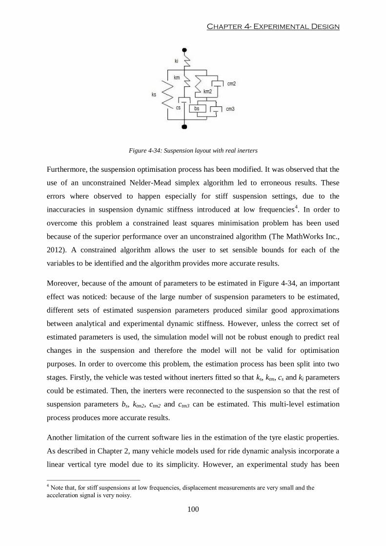
Chapter 4- Experimental Design
100
Figure 4-34: Suspension layout with real inerters
Furthermore, the suspension optimisation process has been modified. It was observed that the
use of an unconstrained Nelder-Mead simplex algorithm led to erroneous results. These
errors where observed to happen especially for stiff suspension settings, due to the
inaccuracies in suspension dynamic stiffness introduced at low frequencies4. In order to
overcome this problem a constrained least squares minimisation problem has been used
because of the superior performance over an unconstrained algorithm (The MathWorks Inc.,
2012). A constrained algorithm allows the user to set sensible bounds for each of the
variables to be identified and the algorithm provides more accurate results.
Moreover, because of the amount of parameters to be estimated in Figure 4-34, an important
effect was noticed: because of the large number of suspension parameters to be estimated,
different sets of estimated suspension parameters produced similar good approximations
between analytical and experimental dynamic stiffness. However, unless the correct set of
estimated parameters is used, the simulation model will not be robust enough to predict real
changes in the suspension and therefore the model will not be valid for optimisation
purposes. In order to overcome this problem, the estimation process has been split into two
stages. Firstly, the vehicle was tested without inerters fitted so that ks, ktm, cs and ki parameters
could be estimated. Then, the inerters were reconnected to the suspension so that the rest of
suspension parameters bs, ktm2, ctm2 and ctm3 can be estimated. This multi-level estimation
process produces more accurate results.
Another limitation of the current software lies in the estimation of the tyre elastic properties.
As described in Chapter 2, many vehicle models used for ride dynamic analysis incorporate a
linear vertical tyre model due to its simplicity. However, an experimental study has been
4 Note that, for stiff suspensions at low frequencies, displacement measurements are very small and the
acceleration signal is very noisy.

Optimisation of racing car suspensions featuring inerters
101
carried out in this research work to assess the validity of this assumption. In this study, tyre
stiffness and damping characteristics was been obtained from experimental data using a
similar procedure as the one used for estimating suspension parameters. According to this,
the general dynamic stiffness Ktyre_dyn of any tyre can be calculated as follows:
Where CPL represents the measured dynamic tyre load and xtyre represents tyre deflection.
This tyre deflection xtyre can be experimentally obtained as follows:
Where xinput is the measured input displacement recorded from actuator displacement sensor
and xu represents the unsprung mass displacement and can be obtained from measured hub
acceleration .
When working in the frequency domain, the dynamic tyre stiffness Ktyre_dyn can be expressed
as a complex number z=a+bωj. For general vibrations theory, the real part of this complex
number represents the elastic term of the system and the imaginary part represents the
damping term. Therefore, tyre stiffness kt and tyre damping ct can be obtained as follows:
Figure 4-35 shows an example of the estimated tyre stiffness kt versus tyre deflection xt
obtained from the process explained above for a vehicle with and without inerters. A similar
behaviour can be obtained when tyre damping ct is plotted against the rate of tyre deflection
. A number of conclusions can be drawn from this study: firstly, tyre characteristics
do not exhibit a linear behaviour. Results suggest that some interaction exists between the
tyre characteristic and the tyre deflection regardless of the type of suspension used. Causes
for this behaviour could reside in the complex construction of a tyre, nonlinear elastic
behaviour of the rubber that composes the tyre’s tread and/or variations in the local pressure
at the contact patch due to dynamic vibration. Secondly, it can be observed that tyres are
subjected to much higher deflections when suspensions incorporate inerters. This is due to the
fact that, as concluded in Chapter 3, inerters cause an increase of vibration transmissibility
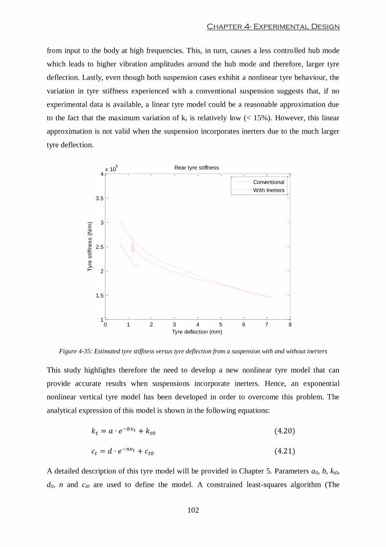
Chapter 4- Experimental Design
102
from input to the body at high frequencies. This, in turn, causes a less controlled hub mode
which leads to higher vibration amplitudes around the hub mode and therefore, larger tyre
deflection. Lastly, even though both suspension cases exhibit a nonlinear tyre behaviour, the
variation in tyre stiffness experienced with a conventional suspension suggests that, if no
experimental data is available, a linear tyre model could be a reasonable approximation due
to the fact that the maximum variation of kt is relatively low (< 15%). However, this linear
approximation is not valid when the suspension incorporates inerters due to the much larger
tyre deflection.
Figure 4-35: Estimated tyre stiffness versus tyre deflection from a suspension with and without inerters
This study highlights therefore the need to develop a new nonlinear tyre model that can
provide accurate results when suspensions incorporate inerters. Hence, an exponential
nonlinear vertical tyre model has been developed in order to overcome this problem. The
analytical expression of this model is shown in the following equations:
A detailed description of this tyre model will be provided in Chapter 5. Parameters a0, b, kt0,
d0, n and ct0 are used to define the model. A constrained least-squares algorithm (The
0 1 2 3 4 5 6 7 81
1.5
2
2.5
3
3.5
4x 10
5
Tyre deflection (mm)
Tyre
stiff
ness (
N/m
)
Rear tyre stiffness
Conventional
With Inerters

Optimisation of racing car suspensions featuring inerters
103
MathWorks Inc., 2012) has been used to fit the tyre model presented in equations (4.20) and
(4.21) and therefore to obtain an estimation of these parameters.
Finally, further extensions to the original parameter estimation software (Bennett, 2012)
comprise the inclusion of new FRFs for dynamic front and rear ride heights and dynamic
longitudinal weight distribution variation. According to this, an expression for front and rear
dynamic ride heights RH has been obtained as follows:
Where xsi represents the displacement of the sprung mass at the axle i and can be obtained
from measured body acceleration by either double-integrating the time domain signal or
by dividing by ω2 the frequency domain signal. xinputi represents the measured actuator
displacement at the axle i and.
Moreover, the dynamic longitudinal weight distribution variation WDist_Dyn can be
expressed as follows:
Where CPLF, CPLR represent front and rear dynamic loads at the tyre contact patch
respectively.
These FRFs will be used in later chapters of this research work to create performance based
objective functions for suspension optimisation.
Chapter 4- Experimental Design
104
4.6. Summary
The design and description of the practical inerters incorporated as part of the test vehicle and
the experimental apparatus used in this research work has been presented and discussed in
this chapter. In order to study the behaviour of a suspension fitted inerters experimentally, an
old Formula Student chassis has been used as a test car. This test car required some re-design
in order to accommodate all the new suspension components. Moreover, real inerters needed
to be designed and manufactured. The design process from the identification of a need to the
delivery of the final product, i.e. a test vehicle incorporating real inerters, has been described.
Furthermore, the Multimatic four-post rig is the test facility presented to test the new
suspension featuring inerters in this thesis. The main components of this facility including the
hydraulic, instrumentation and control systems have been described and the operating
principle of the rig has been discussed.
Finally, the current suspension analysis and parameter estimation software was developed by
Bennett (2012). The key features of the software were described and extensions were
proposed to account for real inerters and nonlinear tyres. This extended parameter estimation
software is used extensively in the work described in Chapter 5 in order to estimate vehicle,
suspension and tyre experimental parameters from the test car incorporating real inerters
designed in this chapter and to validate the new virtual vehicle model against experimental
data from four-post rig testing.
Optimisation of racing car suspensions featuring inerters
105
5. Vehicle Suspension Modelling and Validation
5.1. Introduction
Vehicle models are theoretical representations based on mathematical expression of the
physical working principles of an actual vehicle. Simulation models are powerful tools for
virtual analysis and optimisation. These models allow vehicle engineers to study and
investigate new improved solutions long before the car is manufactured. Furthermore, since
there is no need of track data for simulation, they do not require a complete full-scale
physical prototype to be built. Hence, vehicle simulation and modelling is cost and time
effective.
Depending on the level of analysis required and the stage of the process design, vehicle
models can range from very simple theoretical approximations to highly complex vehicle
dynamics representations. When determining the model complexity, a compromised solution
must be selected based on usefulness, accuracy and computational effort. In this research
work, a vehicle model has been developed in order to fulfil two main objectives: the first
objective is to analyse the ride dynamics of a race car suspension featuring inerters; and the
second is to develop an algorithm for suspension optimisation. In order to analyse and
optimise vehicle suspensions with some degree of reliability, the simulation model must be
capable of replicating the dynamic behaviour of the physical system.
In this chapter, an investigation into the simulation capabilities of different commercial
modelling software packages has been carried out in order to determine the software
framework in which vehicle models will be developed. Before proceeding with the
development of the suspension layout, different levels of model complexity have been
considered with regard to usefulness, accuracy and computational requirements. Finally, a
vehicle model that accounts for real inerters and nonlinear tyres has been developed and
validated with experimental data obtained from four-post rig testing. Discussions with regard
to model accuracy and possible sources of error have been carried out.

Chapter 5- Vehicle Suspension Modelling and Simulation
106
5.2. Selection of the most suitable Modelling Software
Several commercial software packages are available for the design and development of
vehicle models for simulation. A study with a simple linear 4-DOF half-car model (see
Figure 5-1) has been carried out in order to determine the most suitable commercial software
to be used in the present thesis.
Figure 5-1: 4-DOF Half Car model
Three different commercial software packages were analysed:
MSC.Adams
Simulink
SimMechanics
MSC.Adams is a software package dedicated to the analysis and simulation of mechanical
systems. MSC.Adams allows the creation of mechanical multi-body dynamic (MBD) systems
by the definition of objects, joints and motion within a three dimensional environment.
(MscSoftware, 2012).
Simulink is an environment for multi-domain simulation and Model-Based Design for
dynamic and embedded systems. It provides an interactive graphical environment and a
customizable set of block libraries that let you design, simulate, implement, and test a variety
of time-varying systems. Simulink operates under the platform of MatLab. Full interaction
between MatLab and Simulink is possible (MathWorks, 2012).
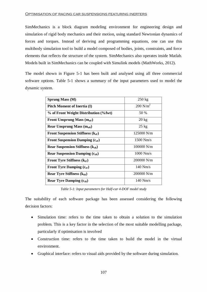
Optimisation of racing car suspensions featuring inerters
107
SimMechanics is a block diagram modeling environment for engineering design and
simulation of rigid body mechanics and their motion, using standard Newtonian dynamics of
forces and torques. Instead of deriving and programming equations, one can use this
multibody simulation tool to build a model composed of bodies, joints, constraints, and force
elements that reflects the structure of the system. SimMechanics also operates inside Matlab.
Models built in SimMechanics can be coupled with Simulink models (MathWorks, 2012).
The model shown in Figure 5-1 has been built and analysed using all three commercial
software options. Table 5-1 shows a summary of the input parameters used to model the
dynamic system.
Sprung Mass (M) 250 kg
Pitch Moment of Inertia (I) 200 N/m2
% of Front Weight Distribution (%fwt) 50 %
Front Unsprung Mass (muF) 20 kg
Rear Unsprung Mass (muR) 25 kg
Front Suspension Stiffness (ksF) 125000 N/m
Front Suspension Damping (csF) 1500 Nm/s
Rear Suspension Stiffness (ksR) 100000 N/m
Rear Suspension Damping (csR) 1000 Nm/s
Front Tyre Stiffness (ktF) 200000 N/m
Front Tyre Damping (ctF) 140 Nm/s
Rear Tyre Stiffness (ktR) 200000 N/m
Rear Tyre Damping (ctR) 140 Nm/s
Table 5-1: Input parameters for Half-car 4-DOF model study
The suitability of each software package has been assessed considering the following
decision factors:
Simulation time: refers to the time taken to obtain a solution to the simulation
problem. This is a key factor in the selection of the most suitable modelling package,
particularly if optimisation is involved
Construction time: refers to the time taken to build the model in the virtual
environment.
Graphical interface: refers to visual aids provided by the software during simulation.
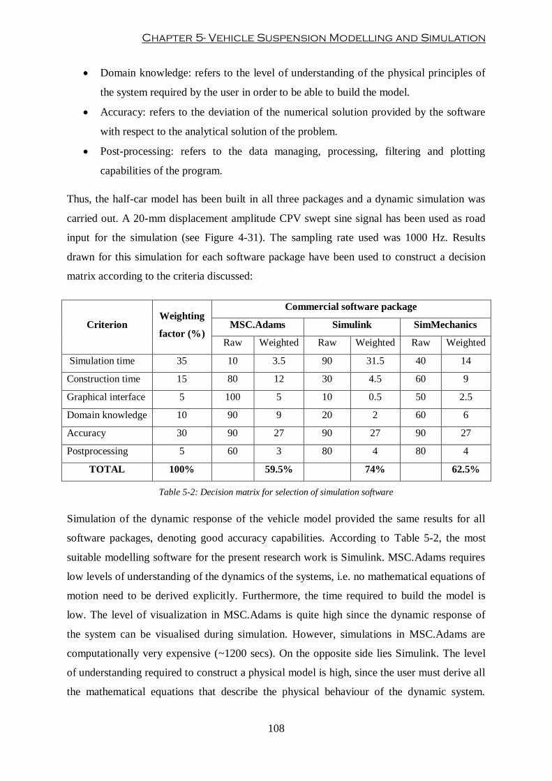
Chapter 5- Vehicle Suspension Modelling and Simulation
108
Domain knowledge: refers to the level of understanding of the physical principles of
the system required by the user in order to be able to build the model.
Accuracy: refers to the deviation of the numerical solution provided by the software
with respect to the analytical solution of the problem.
Post-processing: refers to the data managing, processing, filtering and plotting
capabilities of the program.
Thus, the half-car model has been built in all three packages and a dynamic simulation was
carried out. A 20-mm displacement amplitude CPV swept sine signal has been used as road
input for the simulation (see Figure 4-31). The sampling rate used was 1000 Hz. Results
drawn for this simulation for each software package have been used to construct a decision
matrix according to the criteria discussed:
Criterion Weighting
factor (%)
Commercial software package
MSC.Adams Simulink SimMechanics
Raw Weighted Raw Weighted Raw Weighted
Simulation time 35 10 3.5 90 31.5 40 14
Construction time 15 80 12 30 4.5 60 9
Graphical interface 5 100 5 10 0.5 50 2.5
Domain knowledge 10 90 9 20 2 60 6
Accuracy 30 90 27 90 27 90 27
Postprocessing 5 60 3 80 4 80 4
TOTAL 100% 59.5% 74% 62.5%
Table 5-2: Decision matrix for selection of simulation software
Simulation of the dynamic response of the vehicle model provided the same results for all
software packages, denoting good accuracy capabilities. According to Table 5-2, the most
suitable modelling software for the present research work is Simulink. MSC.Adams requires
low levels of understanding of the dynamics of the systems, i.e. no mathematical equations of
motion need to be derived explicitly. Furthermore, the time required to build the model is
low. The level of visualization in MSC.Adams is quite high since the dynamic response of
the system can be visualised during simulation. However, simulations in MSC.Adams are
computationally very expensive (~1200 secs). On the opposite side lies Simulink. The level
of understanding required to construct a physical model is high, since the user must derive all
the mathematical equations that describe the physical behaviour of the dynamic system.
Optimisation of racing car suspensions featuring inerters
109
Hence, the construction time is also high. No physical visualization of the system is provided
in Simulink. However, once the model is built, simulations run very fast in Simulink (< 1sec).
SimMechanics offers intermediate capabilities between MSC.Adams and Simulink. All
commercial packages offer good data post-processing capabilities, although the fact that
Simulink and SimMechanics operate in Matlab provides more flexibility when manipulating
data. In this thesis, since suspension models are used for optimisation purposes, the most
suitable modelling software is then Simulink.
5.3. Selection of the most suitable Model Complexity
Chapter 2 presented a review of different vehicle suspension models found in the literature.
Reported vehicle suspension models range from linear SDOF systems to complex non-linear
multi-DOF systems. One of the main goals of the present research work is to develop an
experimentally validated vehicle suspension model. This vehicle model must be used for
suspension parameter estimation and suspension optimisation.
According to this, the model must allow the determination of experimental parameters from
four-post rig testing. The vehicle model must account for all the primary motions that can be
measured on a four-post rig test facility. This means that the model will require the definition
of as many degrees of freedom as motions can be reproduced on laboratory testing. The
model must present a level of complexity so that the dynamics of the physical vehicle can be
replicated and the parameter identification method can be applied to any vehicle regardless of
its particular suspension configuration.

Chapter 5- Vehicle Suspension Modelling and Simulation
110
Increasing model complexity can have a number of potential drawbacks. More complex
vehicle models require the estimation of more parameters to be estimated from experimental
data. As explained in Chapter 4, as the number of modelled parameters increases, the
estimation task becomes increasingly complex and inherently prone to estimation error.
Moreover, complex models require longer times to compute the numerical integration of the
dynamic system. This computational time will have a critical impact on the efficiency of the
optimisation algorithm, since the vehicle model must be simulated several times to produce
an optimal solution.
In this thesis, a lumped parameter dynamic vehicle model has been developed. This model
represents only the general dynamic response of vehicle and is not intended to simulate
detailed kinematic movement of each component. In this vehicle representation, chassis,
driver, engine, gearbox and other vehicle systems mounted onto the chassis have been
assumed to be clustered in one rigid body with homogeneous mass and inertia properties.
This simplification is valid as long as the components of the sprung mass are solidly fixed to
the chassis and they are not excited within the frequency range of study. Unsprung masses
have been modelled as lumped masses and they have been constrained to move only in
vertical direction. In real vehicles, the unsprung mass is composed of many elements such as
tyre compound, wheel rim, wheel carrier, brake calliper, part of the suspension arms and part
of the suspension dynamic devices. Moreover, the movement of the wheel is not constrained
to only vertical motion; instead, wheels describe a 3D trajectory in space. Furthermore,
structural deflection of sprung and unsprung masses have been neglected. In a lumped
parameter vehicle model, masses are modelled as infinitely stiff bodies and deflection is only
produced by massless elastic components such as suspensions and tyres.
The following sub-sections discuss the complexity of the vehicle models selected for
parameter estimation and optimisation according to the model design premises presented.
5.3.1. Vehicle suspension model complexity for Parameter Estimation
As mentioned in section 4.5.1, the main modes of vibration that can be reproduced on a four-
post rig test facility are heave, pitch, roll and warp or articulation. The simplest model that
would reproduce these motions would be a system composed by a solid-rigid body attached
to the excitation source via 4 elastic links (see Figure 5-2). Such a system has 3 degrees of
freedom.
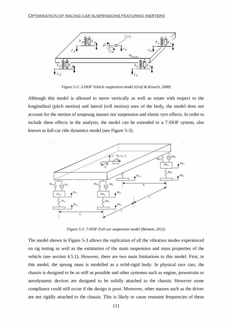
Optimisation of racing car suspensions featuring inerters
111
Figure 5-2: 3-DOF Vehicle suspension model (Graf & Kosuch, 2008)
Although this model is allowed to move vertically as well as rotate with respect to the
longitudinal (pitch motion) and lateral (roll motion) axes of the body, the model does not
account for the motion of unsprung masses nor suspension and elastic tyre effects. In order to
include these effects in the analysis, the model can be extended to a 7-DOF system, also
known as full-car ride dynamics model (see Figure 5-3).
Figure 5-3: 7-DOF Full-car suspension model (Bennett, 2012)
The model shown in Figure 5-3 allows the replication of all the vibration modes experienced
on rig testing as well as the estimation of the main suspension and mass properties of the
vehicle (see section 4.5.1). However, there are two main limitations to this model. First, in
this model, the sprung mass is modelled as a solid-rigid body. In physical race cars, the
chassis is designed to be as stiff as possible and other systemss such as engine, powertrain or
aerodynamic devices are designed to be solidly attached to the chassis. However some
compliance could still occur if the design is poor. Moreover, other masses such as the driver
are not rigidly attached to the chassis. This is likely to cause resonant frequencies of these
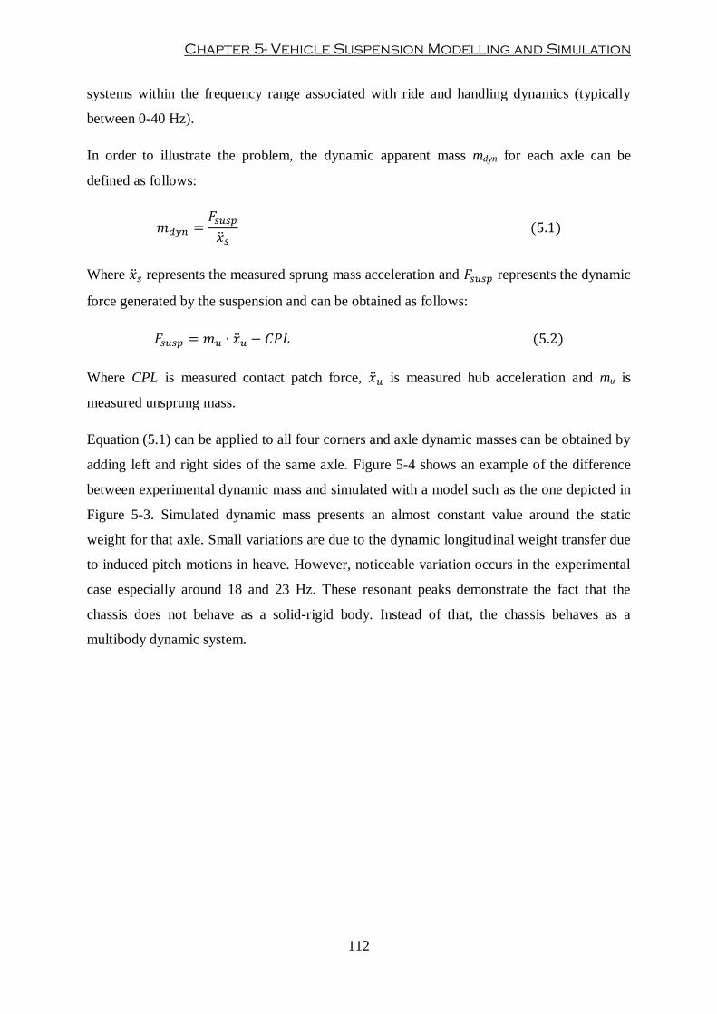
Chapter 5- Vehicle Suspension Modelling and Simulation
112
systems within the frequency range associated with ride and handling dynamics (typically
between 0-40 Hz).
In order to illustrate the problem, the dynamic apparent mass mdyn for each axle can be
defined as follows:
Where represents the measured sprung mass acceleration and represents the dynamic
force generated by the suspension and can be obtained as follows:
Where CPL is measured contact patch force, is measured hub acceleration and mu is
measured unsprung mass.
Equation (5.1) can be applied to all four corners and axle dynamic masses can be obtained by
adding left and right sides of the same axle. Figure 5-4 shows an example of the difference
between experimental dynamic mass and simulated with a model such as the one depicted in
Figure 5-3. Simulated dynamic mass presents an almost constant value around the static
weight for that axle. Small variations are due to the dynamic longitudinal weight transfer due
to induced pitch motions in heave. However, noticeable variation occurs in the experimental
case especially around 18 and 23 Hz. These resonant peaks demonstrate the fact that the
chassis does not behave as a solid-rigid body. Instead of that, the chassis behaves as a
multibody dynamic system.

Optimisation of racing car suspensions featuring inerters
113
Figure 5-4: Dynamic apparent mass comparison – experimental data and 7-DOF model
Bennett (2012) investigated a chassis composed of several masses. Results suggested that the
addition of extra DOFs could lead to a more accurate dynamic representation of the physical
vehicle. However, the increased complexity of this model would also increase the simulation
time and additional instrumentation would be required to determine properties (mass,
location, elastic terms) of the new bodies.
In addition to this, a study has been carried out to analyse the impact of a simplified 1-DOF
chassis when validating a vehicle model with experimental data obtained from physical car.
A linear 7-DOF full-car model has been used to estimate the parameters of the test car
featuring conventional suspensions without inerters. Using the method for parameter
identification explained in Chapter 4, a set of vehicle and suspension parameters have been
obtained. These estimated parameters have then been used to compare the response of model
against experimental data. Validation results are shown in Figure 5-5 and Figure 5-6.
5 10 15 20 25 300
50
100
150Front Apparent Mass Amplitude response
Am
plit
ude r
atio
Simulation
Exp Rig Data
5 10 15 20 25 3050
100
150
200
250Rear Apparent Mass Amplitude response
Frequency(Hz)
Am
plit
ude r
atio
Appare
nt M
ass (
kg)
Appare
nt M
ass (
kg)
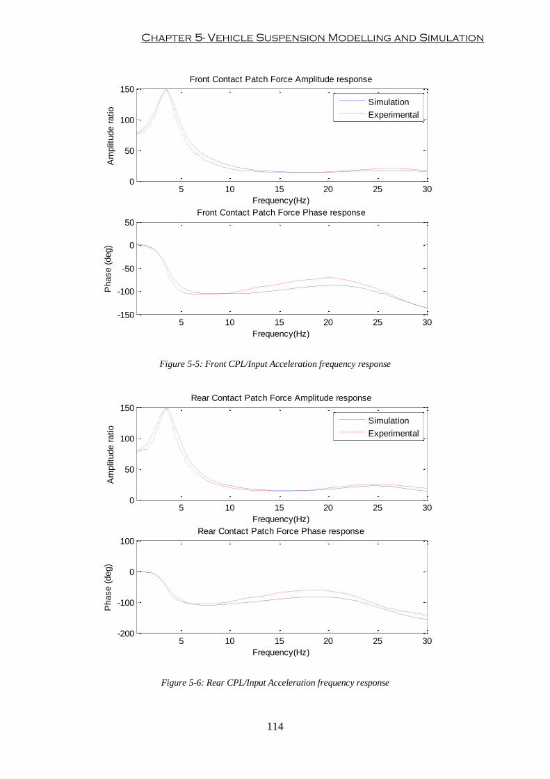
Chapter 5- Vehicle Suspension Modelling and Simulation
114
Figure 5-5: Front CPL/Input Acceleration frequency response
Figure 5-6: Rear CPL/Input Acceleration frequency response
5 10 15 20 25 300
50
100
150Front Contact Patch Force Amplitude response
Frequency(Hz)
Am
plit
ude r
atio
Simulation
Experimental
5 10 15 20 25 30-150
-100
-50
0
50Front Contact Patch Force Phase response
Frequency(Hz)
Phase (
deg)
5 10 15 20 25 300
50
100
150Rear Contact Patch Force Amplitude response
Frequency(Hz)
Am
plit
ude r
atio
Simulation
Experimental
5 10 15 20 25 30-200
-100
0
100Rear Contact Patch Force Phase response
Frequency(Hz)
Phase (
deg)
Optimisation of racing car suspensions featuring inerters
115
Figure 5-5 and Figure 5-6 show that, even though the apparent mass estimation (see Figure
5-4) is not accurate, a 7-DOF model can still replicate the dynamic behaviour of the system.
According to this, it has been decided that the chassis will be modelled as a single solid-rigid
body.
The other limitation is the roll response of the system. A 7-DOF model assumes that the body
will roll about the CoG of the vehicle. Moreover, this model assumes no lateral friction of the
tyres during the roll response. When testing on the rig, Polytetrafluoroethylene (PFTE) pads
are fitted on top of the steel pads to reduce the lateral friction between contact patch and pad.
However, even with the pads fitted, there is still noticeable friction. In order to accurately
represent this motion, the model should account for roll centre and lateral tyre compliance.
Moreover, Bennett (2012) demonstrated that the effect of non-rotating wheels has a major
impact in the roll response of a vehicle. The study carried out in that research work suggested
that the dynamic roll response of the system is velocity dependent. Therefore, correlation
between simulation and rig data would not be representative of the real behaviour of the car
on a race track. According to this, the roll response in this research work will be used only for
parameter identification purposes. Moreover, the roll response of vehicle will not be
considered when defining performance based objective functions for suspension optimisation
in Chapter 7.
5.3.2. Vehicle suspension model for Optimisation
As discussed in Chapter 2, the suspension optimisation problem requires the minimisation of
a cost function J (or a set of cost functions in the case of MOOP) with respect to a set of
suspension variables X. The evaluation of this objective function J requires the numerical
integration of the set of EOMs that describe the dynamic behaviour of the vehicle system.
Hence, the overall computational efficiency of the optimisation solver depends highly on the
simulation time of the vehicle model.
As mentioned in Chapter 4, the vehicle has been designed to be symmetric with respect to its
longitudinal axis. Furthermore, the roll response of a vehicle on the rig is not representative
of the roll behaviour of the physical vehicle on a race track due to the effect of non-rotating
wheels. Thus, roll dynamics has been neglected in the study of suspension performance. For
these reasons, the vehicle model used in parameter estimation can be simplified to a 4-DOF
half-car model when roll motion is neglected.

Chapter 5- Vehicle Suspension Modelling and Simulation
116
This simplification presents two main advantages. Firstly, the simplified model has faster
simulation time. Since a half-car model has less state variables to be computed during the
numerical integration process than a full-car model, increased computational efficiency can
be achieved. A performance test was carried out to study the sensitivity of simulation time to
the complexity of the model. In this study, a constant peak velocity (CPV) sine swept signal
was used as model input. Both, full-car and half-car, models are simulated for 60 seconds
with a sampling rate of 200 Hz. Three identical simulations are run for each model and
simulation times are averaged. Results of this study are summarised in the following table:
Simulation Time (secs)
Full-car model Half-car model
Run 1 2.45 0.65
Run 2 2.41 0.66
Run 3 2.47 0.67
Average 2.44 0.66
Table 5-3: Simulation time comparison – Full-car and Half-car models
Table 5-3 shows that simulation time can be decreased from 2.44 to 0.66 seconds. This means
that the optimisation process could converge to an optimal solution almost four times faster.
Secondly, the other advantage of the use of a simplified vehicle model in optimisation is
related to the definition of the optimisation search space X. A half-car model assumes equal
left-to-right suspension parameters. This means that the number of suspension parameters
that compose the search space X can be halved with respect to the full vehicle model. Hence,
the computational efficiency of the optimisation solver can be increased further.
5.4. Modelling Suspension System Features
The main objective in vehicle suspension modelling is to obtain a reliable model for
simulation. A vehicle model is useful only if it can accurately represent the real system and if
it can reliably predict changes in the dynamic response according to different suspension
settings.
In this section, a comprehensive vehicle suspension model has been developed so that it
could be broadly applied to different race car suspension configurations. The model accounts
for not only the main linear suspension components but also suspension parasitic effects and
nonlinear tyres.
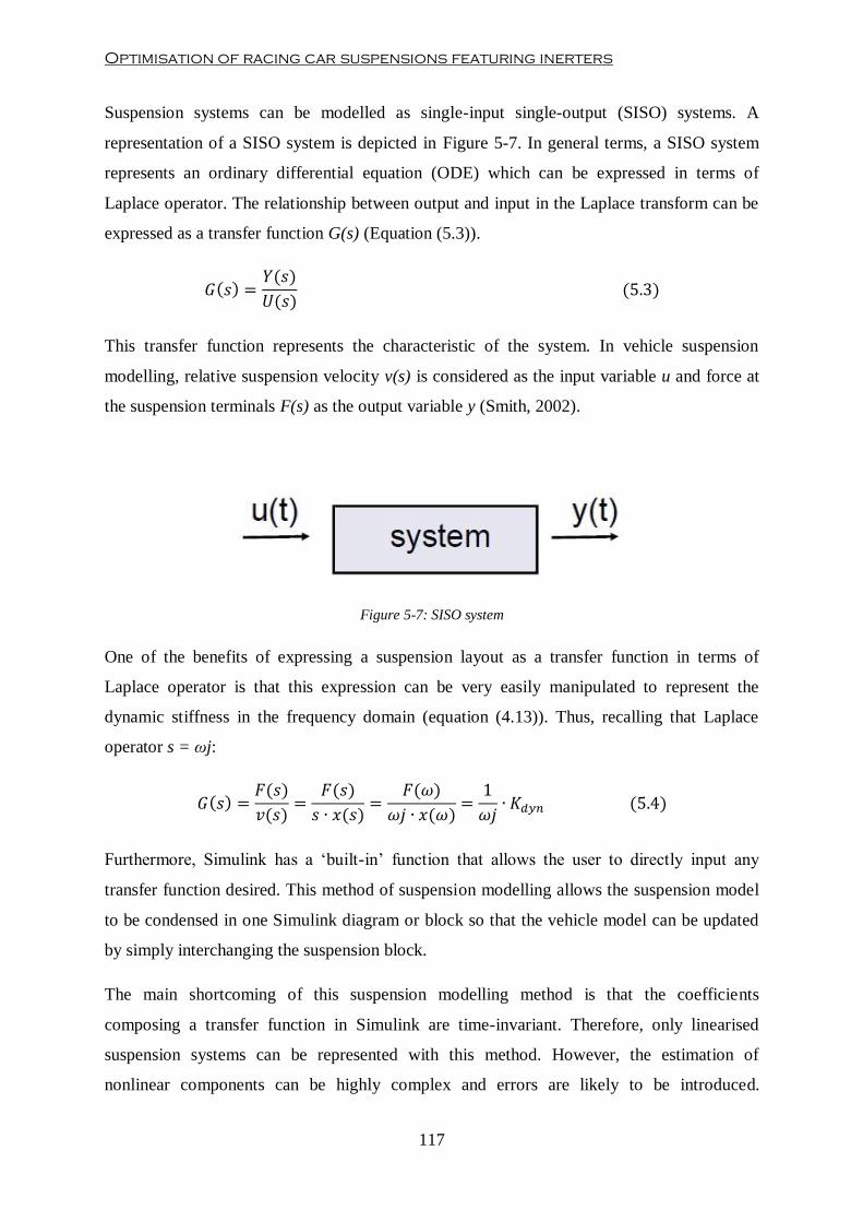
Optimisation of racing car suspensions featuring inerters
117
Suspension systems can be modelled as single-input single-output (SISO) systems. A
representation of a SISO system is depicted in Figure 5-7. In general terms, a SISO system
represents an ordinary differential equation (ODE) which can be expressed in terms of
Laplace operator. The relationship between output and input in the Laplace transform can be
expressed as a transfer function G(s) (Equation (5.3)).
This transfer function represents the characteristic of the system. In vehicle suspension
modelling, relative suspension velocity v(s) is considered as the input variable u and force at
the suspension terminals F(s) as the output variable y (Smith, 2002).
Figure 5-7: SISO system
One of the benefits of expressing a suspension layout as a transfer function in terms of
Laplace operator is that this expression can be very easily manipulated to represent the
dynamic stiffness in the frequency domain (equation (4.13)). Thus, recalling that Laplace
operator s = ωj:
Furthermore, Simulink has a ‘built-in’ function that allows the user to directly input any
transfer function desired. This method of suspension modelling allows the suspension model
to be condensed in one Simulink diagram or block so that the vehicle model can be updated
by simply interchanging the suspension block.
The main shortcoming of this suspension modelling method is that the coefficients
composing a transfer function in Simulink are time-invariant. Therefore, only linearised
suspension systems can be represented with this method. However, the estimation of
nonlinear components can be highly complex and errors are likely to be introduced.

Chapter 5- Vehicle Suspension Modelling and Simulation
118
Moreover, the addition of suspension nonlinearities will increase model complexity and
computational effort required to simulate it. Hence, in this thesis, the transfer function G(s)
has been used to characterise and model different suspension layouts.
5.4.1. Suspension System Layout featuring Inerters
Chapter 4 introduced and discussed the design of a test suspension incorporating real inerters.
In this suspension system, the inerter has been designed so that it works in parallel with a
conventional suspension, i.e. in parallel with springs and dampers. According to this design,
the simplest suspension model can be composed by the three ideal mechanical elements in
parallel. This suspension model has been labelled as suspension type 1. Such a suspension
layout has been depicted in Figure 5-8.
Figure 5-8: Suspension layout featuring with ideal mechanical elements – Type 1
According to Smith and Wang (2004), the characteristic equation of a suspension system can
be expressed as the admittance of the mechanical system. Following the force-current
analogy, the characteristic transfer function of the suspension layout shown in Figure 5-8 can
be expressed as follows:
Where k is the spring stiffness, c is the damping coefficient and b is the inertance coefficient
of the suspension.
The characteristic transfer function of equation (5.5) can then be used to obtain the simulated
dynamic stiffness in the frequency domain following the procedure of equation (5.4). This
theoretical response can then be correlated against experimental dynamic stiffness obtained
from rig testing. In order to do so, the physical vehicle was tested incorporating real inerters
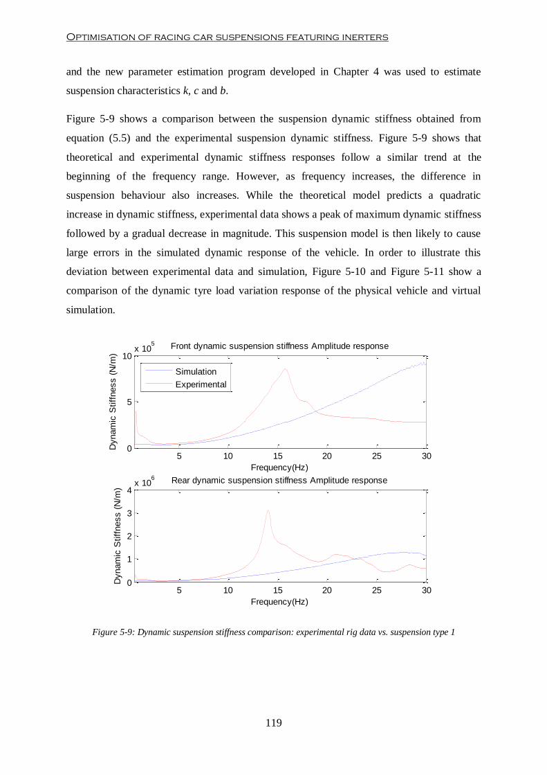
Optimisation of racing car suspensions featuring inerters
119
and the new parameter estimation program developed in Chapter 4 was used to estimate
suspension characteristics k, c and b.
Figure 5-9 shows a comparison between the suspension dynamic stiffness obtained from
equation (5.5) and the experimental suspension dynamic stiffness. Figure 5-9 shows that
theoretical and experimental dynamic stiffness responses follow a similar trend at the
beginning of the frequency range. However, as frequency increases, the difference in
suspension behaviour also increases. While the theoretical model predicts a quadratic
increase in dynamic stiffness, experimental data shows a peak of maximum dynamic stiffness
followed by a gradual decrease in magnitude. This suspension model is then likely to cause
large errors in the simulated dynamic response of the vehicle. In order to illustrate this
deviation between experimental data and simulation, Figure 5-10 and Figure 5-11 show a
comparison of the dynamic tyre load variation response of the physical vehicle and virtual
simulation.
Figure 5-9: Dynamic suspension stiffness comparison: experimental rig data vs. suspension type 1
5 10 15 20 25 300
5
10x 10
5 Front dynamic suspension stiffness Amplitude response
Frequency(Hz)
Dynam
ic S
tiff
ness (
N/m
)
Simulation
Experimental
5 10 15 20 25 300
1
2
3
4x 10
6 Rear dynamic suspension stiffness Amplitude response
Frequency(Hz)
Dynam
ic S
tiff
ness (
N/m
)

Chapter 5- Vehicle Suspension Modelling and Simulation
120
Figure 5-10: Front CPL frequency response: experimental vs. simulation type 1
Figure 5-11: Rear CPL frequency response: experimental vs. simulation type 1
5 10 15 20 25 300
50
100
150Front Contact Patch Force Amplitude response
Frequency(Hz)
Am
plit
ude r
atio
Simulation
Experimental
5 10 15 20 25 30-200
-150
-100
-50
0
50Front Contact Patch Force Phase response
Frequency(Hz)
Phase (
deg)
5 10 15 20 25 300
50
100
150
200
250Rear Contact Patch Force Amplitude response
Frequency(Hz)
Am
plit
ude r
atio
Simulation
Experimental
5 10 15 20 25 30-200
-150
-100
-50
0
50Rear Contact Patch Force Phase response
Frequency(Hz)
Phase (
deg)
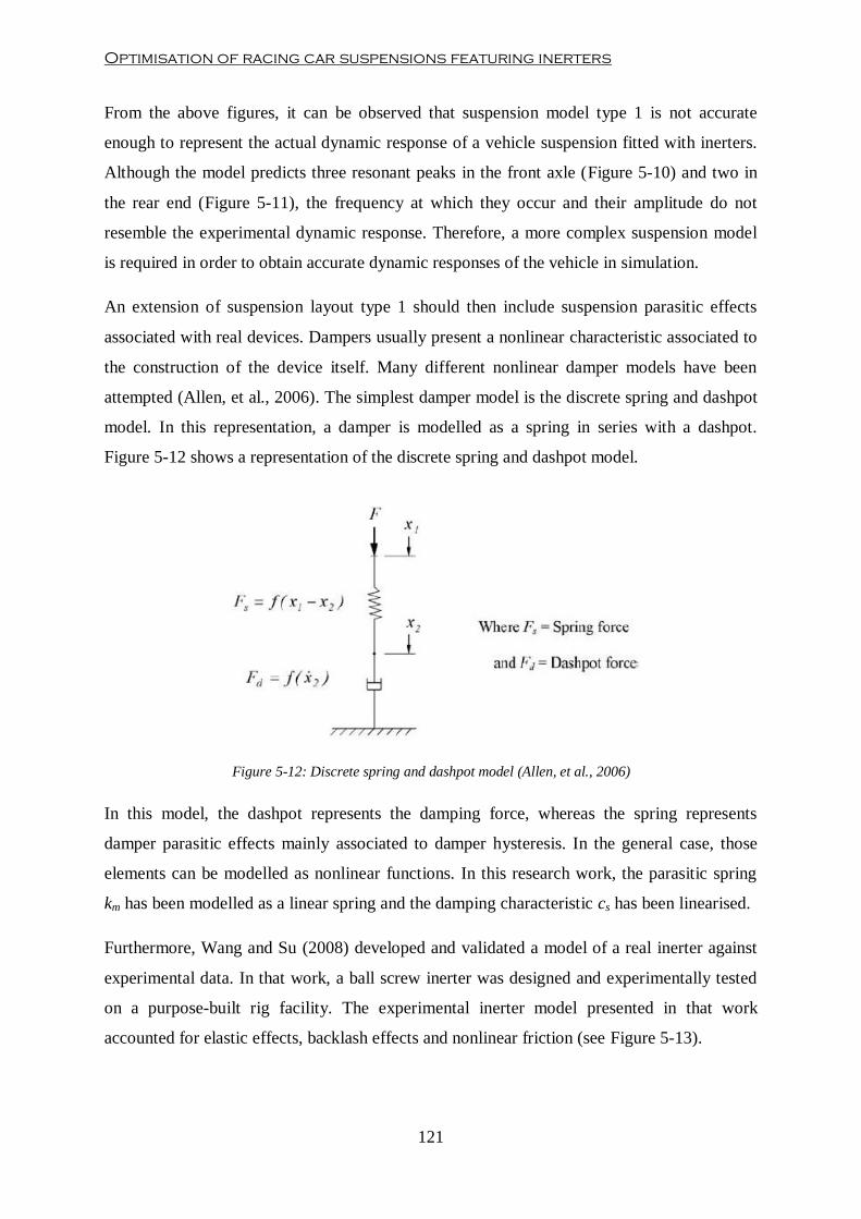
Optimisation of racing car suspensions featuring inerters
121
From the above figures, it can be observed that suspension model type 1 is not accurate
enough to represent the actual dynamic response of a vehicle suspension fitted with inerters.
Although the model predicts three resonant peaks in the front axle (Figure 5-10) and two in
the rear end (Figure 5-11), the frequency at which they occur and their amplitude do not
resemble the experimental dynamic response. Therefore, a more complex suspension model
is required in order to obtain accurate dynamic responses of the vehicle in simulation.
An extension of suspension layout type 1 should then include suspension parasitic effects
associated with real devices. Dampers usually present a nonlinear characteristic associated to
the construction of the device itself. Many different nonlinear damper models have been
attempted (Allen, et al., 2006). The simplest damper model is the discrete spring and dashpot
model. In this representation, a damper is modelled as a spring in series with a dashpot.
Figure 5-12 shows a representation of the discrete spring and dashpot model.
Figure 5-12: Discrete spring and dashpot model (Allen, et al., 2006)
In this model, the dashpot represents the damping force, whereas the spring represents
damper parasitic effects mainly associated to damper hysteresis. In the general case, those
elements can be modelled as nonlinear functions. In this research work, the parasitic spring
km has been modelled as a linear spring and the damping characteristic cs has been linearised.
Furthermore, Wang and Su (2008) developed and validated a model of a real inerter against
experimental data. In that work, a ball screw inerter was designed and experimentally tested
on a purpose-built rig facility. The experimental inerter model presented in that work
accounted for elastic effects, backlash effects and nonlinear friction (see Figure 5-13).

Chapter 5- Vehicle Suspension Modelling and Simulation
122
Figure 5-13: Nonlinear experimental inerter model (Wang & Su, 2008)
The model depicted in Figure 5-13 presents several nonlinearities that cannot be represented
on a transfer function. In this thesis, a new linearised real inerter model is presented instead.
The ball screw model designed and manufactured in this research work has preloaded balls
inside the screw race. This preload prevents the mechanism from having backlash effects
(ε=0). Moreover, inerter friction has been modelled as a linear viscous damping effect Cf.
Finally, compliance effects have been modelled as a linear spring kb (elastic term) in parallel
with a damper Cb (energy dissipation term). These modifications allow the linearization of
the experimental inerter model (see Figure 5-14).
Figure 5-14: Linearised experimental inerter model
Another parasitic effect to take into account is suspension compliance. An important
compromise exists in the design of race car suspension components (e.g. wishbones,
pull/push-rods or rockers). On one hand, suspension components must be stiff enough so that
they are capable of withstanding external forces applied to the chassis through the suspension
system. On the other hand, components must be designed to be as light as possible in order to
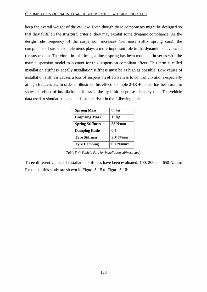
Optimisation of racing car suspensions featuring inerters
123
keep the overall weight of the car low. Even though these components might be designed so
that they fulfil all the structural criteria, they may exhibit some dynamic compliance. As the
design ride frequency of the suspension increases (i.e. more stiffly sprung cars), the
compliance of suspension elements plays a more important role in the dynamic behaviour of
the suspension. Therefore, in this thesis, a linear spring has been modelled in series with the
main suspension model to account for this suspension compliant effect. This term is called
installation stiffness. Ideally installation stiffness must be as high as possible. Low values of
installation stiffness causes a loss of suspension effectiveness to control vibrations especially
at high frequencies. In order to illustrate this effect, a simple 2-DOF model has been used to
show the effect of installation stiffness in the dynamic response of the system. The vehicle
data used to simulate this model is summarised in the following table.
Sprung Mass 65 kg
Unsprung Mass 15 kg
Spring Stiffness 38 N/mm
Damping Ratio 0.4
Tyre Stiffness 250 N/mm
Tyre Damping 0.1 N/mm/s
Table 5-4: Vehicle data for installation stiffness study
Three different values of installation stiffness have been evaluated: 100, 200 and 650 N/mm.
Results of this study are shown in Figure 5-15 to Figure 5-18:

Chapter 5- Vehicle Suspension Modelling and Simulation
124
Figure 5-15: Effect of installation stiffness - Dynamic Stiffness frequency response
Figure 5-16: Effect of installation stiffness - CPL/Static mass frequency response
5 10 15 20 25 30 350
1
2
3x 10
5 Dynamic suspensions stiffness Amplitude response
Frequency(Hz)
Am
plit
ude r
atio
ki=100 N/mm
ki=200 N/mm
ki=650 N/mm
5 10 15 20 25 30 350
20
40
60
80Dynamic suspensions stiffness Phase response
Frequency(Hz)
Phase (
deg)
5 10 15 20 25 30 350
0.5
1
1.5
2Contact Patch Force Amplitude response
Frequency(Hz)
Am
plit
ude r
atio
ki=100 N/mm
ki=200 N/mm
ki=650 N/mm
5 10 15 20 25 30 35-200
-100
0
100Contact Patch Force Phase response
Frequency(Hz)
Phase (
deg)
Stiffness (
N/m
)
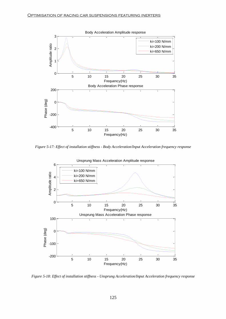
Optimisation of racing car suspensions featuring inerters
125
Figure 5-17: Effect of installation stiffness - Body Acceleration/Input Acceleration frequency response
Figure 5-18: Effect of installation stiffness - Unsprung Acceleration/Input Acceleration frequency response
5 10 15 20 25 30 350
1
2
3Body Acceleration Amplitude response
Frequency(Hz)
Am
plit
ude r
atio
ki=100 N/mm
ki=200 N/mm
ki=650 N/mm
5 10 15 20 25 30 35-400
-200
0
200Body Acceleration Phase response
Frequency(Hz)
Phase (
deg)
5 10 15 20 25 30 350
2
4
6Unsprung Mass Acceleration Amplitude response
Frequency(Hz)
Am
plit
ude r
atio
ki=100 N/mm
ki=200 N/mm
ki=650 N/mm
5 10 15 20 25 30 35-200
-100
0
100Unsprung Mass Acceleration Phase response
Frequency(Hz)
Phase (
deg)
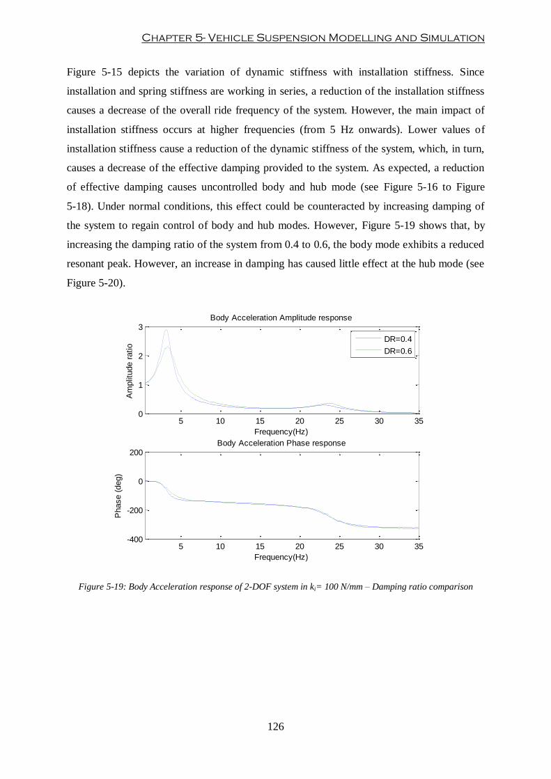
Chapter 5- Vehicle Suspension Modelling and Simulation
126
Figure 5-15 depicts the variation of dynamic stiffness with installation stiffness. Since
installation and spring stiffness are working in series, a reduction of the installation stiffness
causes a decrease of the overall ride frequency of the system. However, the main impact of
installation stiffness occurs at higher frequencies (from 5 Hz onwards). Lower values of
installation stiffness cause a reduction of the dynamic stiffness of the system, which, in turn,
causes a decrease of the effective damping provided to the system. As expected, a reduction
of effective damping causes uncontrolled body and hub mode (see Figure 5-16 to Figure
5-18). Under normal conditions, this effect could be counteracted by increasing damping of
the system to regain control of body and hub modes. However, Figure 5-19 shows that, by
increasing the damping ratio of the system from 0.4 to 0.6, the body mode exhibits a reduced
resonant peak. However, an increase in damping has caused little effect at the hub mode (see
Figure 5-20).
Figure 5-19: Body Acceleration response of 2-DOF system in ki= 100 N/mm – Damping ratio comparison
5 10 15 20 25 30 350
1
2
3Body Acceleration Amplitude response
Frequency(Hz)
Am
plit
ude r
atio
DR=0.4
DR=0.6
5 10 15 20 25 30 35-400
-200
0
200Body Acceleration Phase response
Frequency(Hz)
Phase (
deg)

Optimisation of racing car suspensions featuring inerters
127
Figure 5-20: CPL response of 2-DOF system in ki= 100 N/mm – Damping ratio comparison
Hence, the suspension layout type 1 has been extended so that it accounts for all of these
suspension parasitic effects. The new suspension model takes into account hysteretic damper
effects, friction and compliance inerter effects and overall suspension compliance effects
(installation stiffness). This extended suspension model has been labelled as suspension
layout type 2 and has been depicted in Figure 5-21.
Figure 5-21: Suspension model layout type 2
As with suspension layout type 1, because all the elements composing this extended
suspension layout are linear, a suspension transfer function can be obtained. Again the
5 10 15 20 25 30 350
0.5
1
1.5
2Contact Patch Force Amplitude response
Frequency(Hz)
Am
plit
ude r
atio
DR=0.4
DR=0.6
5 10 15 20 25 30 35-200
-100
0
100Contact Patch Force Phase response
Frequency(Hz)
Phase (
deg)
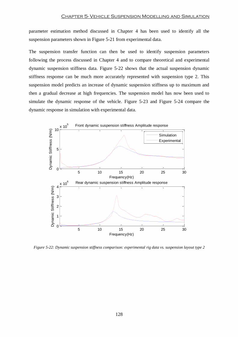
Chapter 5- Vehicle Suspension Modelling and Simulation
128
parameter estimation method discussed in Chapter 4 has been used to identify all the
suspension parameters shown in Figure 5-21 from experimental data.
The suspension transfer function can then be used to identify suspension parameters
following the process discussed in Chapter 4 and to compare theoretical and experimental
dynamic suspension stiffness data. Figure 5-22 shows that the actual suspension dynamic
stiffness response can be much more accurately represented with suspension type 2. This
suspension model predicts an increase of dynamic suspension stiffness up to maximum and
then a gradual decrease at high frequencies. The suspension model has now been used to
simulate the dynamic response of the vehicle. Figure 5-23 and Figure 5-24 compare the
dynamic response in simulation with experimental data.
Figure 5-22: Dynamic suspension stiffness comparison: experimental rig data vs. suspension layout type 2
5 10 15 20 25 300
5
10x 10
5 Front dynamic suspension stiffness Amplitude response
Frequency(Hz)
Dynam
ic S
tiff
ness (
N/m
)
Simulation
Experimental
5 10 15 20 25 300
1
2
3
4x 10
6 Rear dynamic suspension stiffness Amplitude response
Frequency(Hz)
Dynam
ic S
tiff
ness (
N/m
)
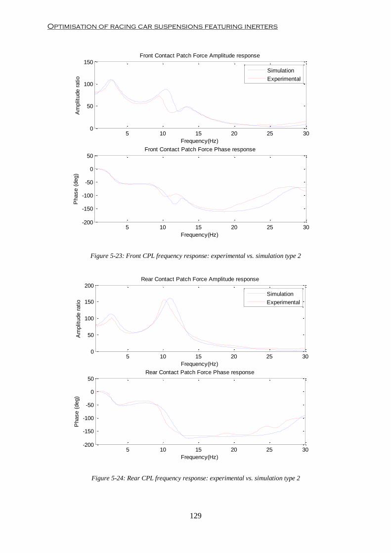
Optimisation of racing car suspensions featuring inerters
129
Figure 5-23: Front CPL frequency response: experimental vs. simulation type 2
Figure 5-24: Rear CPL frequency response: experimental vs. simulation type 2
5 10 15 20 25 300
50
100
150Front Contact Patch Force Amplitude response
Frequency(Hz)
Am
plit
ude r
atio
Simulation
Experimental
5 10 15 20 25 30-200
-150
-100
-50
0
50Front Contact Patch Force Phase response
Frequency(Hz)
Phase (
deg)
5 10 15 20 25 300
50
100
150
200Rear Contact Patch Force Amplitude response
Frequency(Hz)
Am
plit
ude r
atio
Simulation
Experimental
5 10 15 20 25 30-200
-150
-100
-50
0
50Rear Contact Patch Force Phase response
Frequency(Hz)
Phase (
deg)

Chapter 5- Vehicle Suspension Modelling and Simulation
130
Figure 5-23 and Figure 5-24 show better agreement between virtual suspension model and
experimental data than with suspension layout type 1 (see Figure 5-10 and Figure 5-11).
Resonant peaks in simulation occur closer to the peaks found from experimental testing.
However, the simulation model overestimates the amplitude of the hub resonant peak and
there is a drift in the frequency at which the hub mode is occurring. At the beginning, it was
thought that this extended linearised suspension model was not accurate enough. However,
further investigation of the dynamic response of the physical suspension suggested that tyres
were not showing a linear behaviour. Next section focuses on the study of the vertical tyre
model in the dynamic response of the vehicle.
5.4.2. Non-linear Vertical Tyre Modelling
In Chapter 2, literature related to vehicle suspension modelling was discussed. In some of
these vehicle models, tyres were considered as linear springs in order to model the elastic
behaviour of the tyre (Todd & Kulakowski, 1990). Other vehicle models also included
viscous linear tyre damping in order to account for the energy dissipation (Graf & Kosuch,
2008). Although, this is crude approximation of the general highly nonlinear dynamic tyre
behaviour (Pacjeka, 2006), this tyre model has been extensively used in suspension analysis
studies due to its simplicity.
A vehicle model incorporating a conventional suspension (no inerter fitted) and a linear tyre
model has been used to evaluate the behaviour of actual tyres subjected to rig testing. An
experimental test with this suspension configuration was set and tyre characteristics were
estimated following procedure presented in equations (4.16) and (4.17). Figure 5-25 and
Figure 5-26 show a comparison between experimental tyre stiffness and damping (red trace)
and simulation (blue trace) for front and rear axles respectively. Simulated linear tyre
stiffness and damping values have been obtained from an estimated as an average value from
experimental data across the frequency range. As it can be observed in these plots, tyre elastic
properties vary with frequency. Furthermore, experimental data shows that, in the low
frequency range (up to 5 Hz), tyres present low stiffness and high damping characteristics. As
frequency increases tyre stiffness increases and tyre damping decreases.

Optimisation of racing car suspensions featuring inerters
131
Figure 5-25: Front Tyre Stiffness and Damping comparison – Experimental data vs. linear tyre model
Figure 5-26: Rear Tyre Stiffness and Damping comparison – Experimental data vs. linear tyre model
5 10 15 20 25 300
1
2
3
4x 10
5 Front dynamic tyre stiffness
Frequency(Hz)
Dynam
ic S
tiff
ness (
N/m
)
Simulation
Experimental
5 10 15 20 25 30
-2000
0
2000
4000
6000
8000
Front dynamic tyre damping
Frequency(Hz)
Dam
pin
g C
oeff
icie
nt
(Ns/m
)
5 10 15 20 25 30-2
0
2
4x 10
5 Rear dynamic tyre stiffness
Frequency(Hz)
Dynam
ic S
tiff
ness (
N/m
)
Simulation
Experimental
5 10 15 20 25 30
-5000
0
5000
Rear dynamic tyre damping
Frequency(Hz)
Dam
pin
g C
oeff
icie
nt
(Ns/m
)
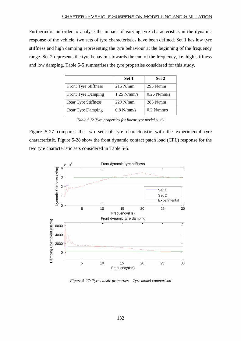
Chapter 5- Vehicle Suspension Modelling and Simulation
132
Furthermore, in order to analyse the impact of varying tyre characteristics in the dynamic
response of the vehicle, two sets of tyre characteristics have been defined. Set 1 has low tyre
stiffness and high damping representing the tyre behaviour at the beginning of the frequency
range. Set 2 represents the tyre behaviour towards the end of the frequency, i.e. high stiffness
and low damping. Table 5-5 summarises the tyre properties considered for this study.
Set 1 Set 2
Front Tyre Stiffness 215 N/mm 295 N/mm
Front Tyre Damping 1.25 N/mm/s 0.25 N/mm/s
Rear Tyre Stiffness 220 N/mm 285 N/mm
Rear Tyre Damping 0.8 N/mm/s 0.2 N/mm/s
Table 5-5: Tyre properties for linear tyre model study
Figure 5-27 compares the two sets of tyre characteristic with the experimental tyre
characteristic. Figure 5-28 show the front dynamic contact patch load (CPL) response for the
two tyre characteristic sets considered in Table 5-5.
Figure 5-27: Tyre elastic properties – Tyre model comparison
5 10 15 20 25 300
1
2
3
4x 10
5 Front dynamic tyre stiffness
Frequency(Hz)
Dynam
ic S
tiff
ness (
N/m
)
Set 1
Set 2
Experimental
5 10 15 20 25 30
0
2000
4000
6000
Front dynamic tyre damping
Frequency(Hz)
Dam
pin
g C
oeff
icie
nt
(Ns/m
)

Optimisation of racing car suspensions featuring inerters
133
Figure 5-28: Front CPL ratio dynamic response with linear tyre mode
Figure 5-28 shows the difference in the CPL dynamic response of the vehicle related to
different tyre models. On one hand, set 1 presents more accuracy in the prediction of the
actual damping of the system at low frequencies (blue trace). However, this set fails to model
the resonant peak at the hub mode. On the other hand, set 2 predicts a more damped body
mode, but it accurately predicts the hub mode (green trace). This means that the vehicle
should feature a variable tyre model that accounts for both sets if high predictive accuracy is
required across the whole frequency range.
A tyre model that is frequency-dependent could be one solution. However, this model does
not contain any information with regard to the phenomena that might cause this apparent
nonlinear behaviour. Moreover, this variable model would only be able to generate accurate
dynamic responses for local suspension configurations, since the estimation would be based
on parameters estimated for a particular suspension system. Further investigation into
nonlinear vertical tyre modelling is then required.
An experimental study of the influence of tyre dynamic deflection into tyre elastic properties
has been carried out. The vehicle was tested on the four-post rig at two different input
displacement amplitudes: 25 and 35 mm. The rest of the suspension parameters remained
5 10 15 20 25 300
50
100
150
200Front Contact Patch Force Amplitude response
Frequency(Hz)
Am
plit
ude r
atio
Set 1
Set 2
Experimental
5 10 15 20 25 30-150
-100
-50
0
50Front Contact Patch Force Phase response
Frequency(Hz)
Phase (
deg)

Chapter 5- Vehicle Suspension Modelling and Simulation
134
unchanged. Experimental tyre deflection and dynamic tyre stiffness responses have been
plotted in Figure 5-30 and Figure 5-29 respectively in order to investigate the interaction
between both magnitudes. In both figures, the blue trace (Run 3 in the legend) represents the
result of the 25-mm input displacement amplitude run and the red trace (Run 7) represents the
result of the 35-mm input displacement amplitude run. As expected, a larger road input
causes larger deflections on the tyre (see Figure 5-29). Interestingly, Figure 5-30 shows that
this increases in tyre deflection cause a reduction of the dynamic tyre stiffness. This suggests
that some interaction between both magnitudes exists.
Figure 5-29: Absolute tyre deflection dynamic response at various input amplitudes
5 10 15 20 25 300
1
2
3Tyre Displacement Amplitude
Frequency (Hz)
Am
plit
ude (
mm
)
Part1 RUN 3 Heave
Part1 RUN 7 Heave
5 10 15 20 25 30-150
-100
-50
0
50Tyre Displacement Phase
Frequency (Hz)
Phase (
degs)
Part1 RUN 3 Heave
Part1 RUN 7 Heave

Optimisation of racing car suspensions featuring inerters
135
Figure 5-30: Experimental dynamic stiffness response for various input amplitudes
Moreover, a pattern between tyre deflection and dynamic stiffness can be observed from the
dynamic responses. At the body mode (3.5 Hz), tyre deflection amplitude reaches its
maximum value, which corresponds to minimum tyre dynamic stiffness. After that, the
amplitude of the absolute tyre deflection gradually reduces (5-15 Hz) until it eventually
reaches a minimum amplitude value. During this frequency range, dynamic stiffness steadily
increases until it settles in a maximum value. In the proximity of the hub mode, tyre
deflection increases again, which leads to a new reduction of the dynamic stiffness.
Therefore, this study demonstrates that tyre elastic properties are tyre deflection dependent
rather than frequency dependent.
Hence, having stated that there is a strong relationship between tyre deflection and tyre
elastic properties, a nonlinear vertical tyre model must be obtained. Assuming that the tyre is
composed by a spring in parallel with a damper, experimental tyre spring and damper
characteristics can be derived from the complex expression of dynamic tyre stiffness.
5 10 15 20 25 300
1
2
3
4x 10
5 Dynamic Tyre Stiffness Responses
Frequency (Hz)
Dynam
ic T
yre
Stiff
ness (
N/m
)
Part1 RUN 3 Heave
Part1 RUN 7 Heave
5 10 15 20 25 30-40
-20
0
20Dynamic Tyre Stiffness Responses
Frequency (Hz)
Phase (
degs)

Chapter 5- Vehicle Suspension Modelling and Simulation
136
Where kt=f(xt) and ct=f(xt) represent nonlinear tyre stiffness and damping respectively and xt
represents the tyre deflection. Note that equation (5.6) is expressed as a complex number in
which the real part represents tyre stiffness kt and the imaginary part represents tyre damping
ct multiplied by the angular frequency ω.
The next step is to plot experimental tyre spring and damping with respect to tyre deflection.
Note that, when modelling dynamic systems, damping elements are defined as devices
capable of generating a force proportional to the relative velocity between component
terminals. According to this, tyre damping will be plotted against tyre deflection rate in
order to keep a consistent definition of the dynamic tyre characteristics with the general
dynamic modelling principles.
Figure 5-31 and Figure 5-32 show the nonlinear tyre stiffness and tyre damping
characteristics obtained from experimental testing respectively. In order to avoid noisy data
due to sensor resolution when measuring small tyre deflections, frequency range has been
limited to regions around body (3-12 Hz) and hub modes (15-28 Hz). The first region
corresponds to maximum tyre deflection and it has been used to plot tyre deflection, whereas
second region corresponds to maximum tyre deflection velocity and it has been used to obtain
an accurate tyre damping estimate. Both tyre stiffness and damping present an exponential
decay characteristic with respect to tyre deflection and tyre deflection velocity respectively.
Figure 5-31: Nonlinear experimental tyre stiffness characteristic: Front (upper) and rear (lower)
0.5 1 1.5 2 2.51.5
2
2.5
3x 10
5
Tyre deflection (mm)
Tyre
stiff
ness (
N/m
)
Front tyre stiffness
0.4 0.6 0.8 1 1.2 1.4 1.6 1.8 2 2.2 2.41.5
2
2.5
3
3.5x 10
5
Tyre deflection (mm)
Tyre
stiff
ness (
N/m
)
Rear tyre stiffness

Optimisation of racing car suspensions featuring inerters
137
Figure 5-32: Nonlinear experimental tyre damping characteristic: Front (upper) and rear (lower)
According to the results obtained in Figure 5-31 and Figure 5-32, a nonlinear exponential tyre
model has been proposed to simulate the actual behaviour of the tyres observed from
experimental testing. Hence, the vertical tyre model can be expressed by the following
equaations:
Equations (5.7) and (5.8) represent a semi-empirical nonlinear vertical tyre model based on
experimental data obtained from four-post rig testing. In those equations, parameters a and d
define the initial values of stiffness and damping respectively. Parameters b and n define the
rate of the exponential decay. Parameters kt0 and ct0 establish an asymptotic bottom limit for
tyre stiffness and damping characteristics and provide numerical consistency to the solver.
All these parameters can be estimated following the procedure explained in Chapter 4. An
experimental test has been carried out so that model correlation can be analysed. A 30-mm
heave run was carried out to the test car fitted with conventional suspension (no inerters
fitted). The value of the parameters obtained from the estimation program have been
summarised in Table 5-6:
0 50 100 150 200 250 3000
500
1000
Tyre deflection velocity(mm/sec)
Tyre
dam
pin
g (
N/m
/s)
Front tyre damping
0 50 100 150 200 250 3000
500
1000
Tyre deflection velocity(mm/sec)
Tyre
dam
pin
g (
N/m
/s)
Rear tyre damping

Chapter 5- Vehicle Suspension Modelling and Simulation
138
Front Tyre Rear Tyre
Tyre Stiffness
a (N/m) 171000 178000
b (mm-1
) 1250 1400
kt0 (N/m) 195000 185000
Tyre Damping
d (Ns/m) 3850 4100
n (s/mm) 45 50
ct0 (Ns/m) 200 350
Table 5-6: Estimated parameters for tyre model
Figure 5-33 and Figure 5-34 show a good correlation between experimental data and the new
nonlinear semi-empirical tyre model developed in this section.
Figure 5-33: Nonlinear tyre stiffness model comparison between experimental vs. exponential model
0 0.5 1 1.5 2 2.51.5
2
2.5
3x 10
5
Tyre deflection (mm)
Tyre
stiff
ness (
N/m
)
Front tyre stiffness
Experimental
Simulation
0 0.5 1 1.5 2 2.51
2
3
4x 10
5
Tyre deflection (mm)
Tyre
stiff
ness (
N/m
)
Rear tyre stiffness
Experimental
Simulation
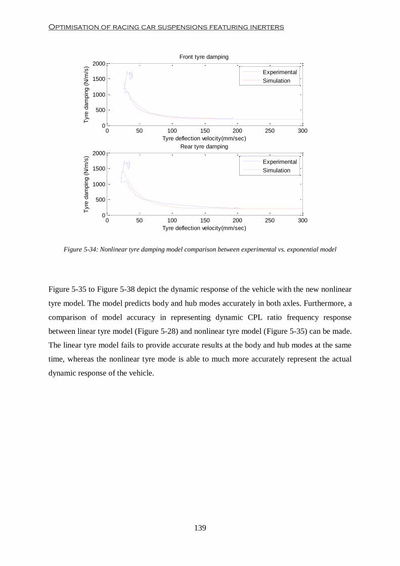
Optimisation of racing car suspensions featuring inerters
139
Figure 5-34: Nonlinear tyre damping model comparison between experimental vs. exponential model
Figure 5-35 to Figure 5-38 depict the dynamic response of the vehicle with the new nonlinear
tyre model. The model predicts body and hub modes accurately in both axles. Furthermore, a
comparison of model accuracy in representing dynamic CPL ratio frequency response
between linear tyre model (Figure 5-28) and nonlinear tyre model (Figure 5-35) can be made.
The linear tyre model fails to provide accurate results at the body and hub modes at the same
time, whereas the nonlinear tyre mode is able to much more accurately represent the actual
dynamic response of the vehicle.
0 50 100 150 200 250 3000
500
1000
1500
2000
Tyre deflection velocity(mm/sec)
Tyre
dam
pin
g (
N/m
/s)
Front tyre damping
Experimental
Simulation
0 50 100 150 200 250 3000
500
1000
1500
2000
Tyre deflection velocity(mm/sec)
Tyre
dam
pin
g (
N/m
/s)
Rear tyre damping
Experimental
Simulation

Chapter 5- Vehicle Suspension Modelling and Simulation
140
Figure 5-35: Front CPL ratio frequency response with nonlinear tyre model
Figure 5-36: Rear CPL frequency ratio response with nonlinear tyre model
5 10 15 20 25 300
50
100
150Front Contact Patch Force Amplitude response
Frequency(Hz)
Am
plit
ude r
atio
Simulation
Experimental
5 10 15 20 25 30-150
-100
-50
0
50Front Contact Patch Force Phase response
Frequency(Hz)
Phase (
deg)
5 10 15 20 25 300
50
100
150Rear Contact Patch Force Amplitude response
Frequency(Hz)
Am
plit
ude r
atio
Simulation
Experimental
5 10 15 20 25 30-150
-100
-50
0
50Rear Contact Patch Force Phase response
Frequency(Hz)
Phase (
deg)
Optimisation of racing car suspensions featuring inerters
141
Figure 5-37: Front unsprung mass acceleration ratio frequency response with nonlinear tyre model
Figure 5-38: Front unsprung mass acceleration ratio frequency response with nonlinear tyre model
5 10 15 20 25 300.5
1
1.5
2Front Unsprung Mass Acceleration Amplitude response
Frequency(Hz)
Am
plit
ude r
atio
Simulation
Experimental
5 10 15 20 25 30-150
-100
-50
0
50Front Unsprung Mass Acceleration Phase response
Frequency(Hz)
Phase (
deg)
5 10 15 20 25 300.5
1
1.5
2Rear Unsprung Mass Acceleration Amplitude response
Frequency(Hz)
Am
plit
ude r
atio
Simulation
Experimental
5 10 15 20 25 30-150
-100
-50
0
50Rear Unsprung Mass Acceleration Phase response
Frequency(Hz)
Phase (
deg)
Chapter 5- Vehicle Suspension Modelling and Simulation
142
Hence, a completed vehicle model can be obtained by integrating this semi-empirical
nonlinear tyre model with the suspension model incorporating real inerters developed in
section 5.4.1. The following section analyses and discusses thoroughly the validity of vehicle
model presented in this section.
5.5. Suspension Validation with 4-Post Rig Test Experimental Results
Simulation models must be validated with experimental data in order to ensure that they are
reproducing the dynamics of the actual vehicle to some degree of accuracy and predictability.
The vehicle model developed in the previous section has been correlated against experimental
data obtained from four-post rig testing. Moreover, the extended parameter estimation
program developed in Chapter 4 has been used to identify vehicle parameters and to analyse
the correlation between the virtual vehicle model and experimental data.
In order to simplify the estimation and the validation process, only suspension settings have
been tuned. The rest of vehicle and tyre properties remained unchanged. Thus, parameters
related to vehicle and tyre properties have not been re-estimated for each suspension setting.
Table 5-7 and Table 5-8 summarises the set of vehicle and tyre properties obtained from the
parameter identification process.
Sprung Mass (ms) 250 kg
Front Unsprung Mass (muf) 14 kg
Rear Unsprung Mass (mur) 15 kg
Front Weight Distribution (%wt) 50.5 %
Pitch Moment of Inertia (Jp) 30.5 kgm2
Roll Moment of Inertia (Jr) 28 kgm2
Wheelbase (l) 1565 mm
Front Track (tf) 1320 mm
Rear Track (tr) 1210 mm
Table 5-7: Vehicle data properties used in validation process
Optimisation of racing car suspensions featuring inerters
143
Front a 171000 N/m
Front b 1250 mm-1
Front kt0 195000 N/m
Front d 3850 Ns/m
Front n 45 s/mm
Front ct0 200 Ns/m
Rear a 178000 N/m
Rear b 1200 mm-1
Rear kt0 185000 N/m
Rear d 4100 Ns/m
Rear n 50 s/mm
Rear ct0 350 Ns/m
Table 5-8: Tyre elastic properties used in validation process
The following sections present the validation graphs and discuss the accuracy of the results
obtained from comparing experimental rig data with simulation.
5.5.1. Analysis of model accuracy for different inerter settings
In order to evaluate accuracy of the model, several suspension configurations have been set
and experimentally tested on the four-post rig. In this way, the model accuracy can be
examined under different conditions and model predictability can also be evaluated.
Over the past sections, the vehicle model incorporating a conventional suspension without
inerters has been used to carry out several analysis studies. These studies demonstrated that
the model was capable of replicating the dynamic behaviour of the physical vehicle. This
section focuses on the analysis of this vehicle model incorporating real inerters and on the
validation of this model against experimental data. Hence, in order to simplify the validation
process, only inerter settings have been modified. According to this, Table 5-9 shows a
tuning sheet with all the suspension settings used in this section. Some general considerations
must be highlighted with regard to the suspension settings selected: firstly, suspension
settings were mirrored from left to right of the test car in order to keep vehicle symmetry with
respect to the longitudinal axis. Secondly, springs and pull/pushrod settings were set so that
the ride frequency of front and rear axles was around 4 and 3.7 Hz respectively. According to
(Milliken & Milliken, 1995), these ride frequencies corresponds to the suspension of race car
with mid/high aerodynamic downforce effects. Lastly, damper settings were selected to

Chapter 5- Vehicle Suspension Modelling and Simulation
144
provide a damping ratio of about 0.45. According to Milliken and Milliken (1995), this
damping ratio offers the optimal road holding performance with a conventional suspension.
Front Springs 500 lbs/in
Rear Springs 500 lbs/in
Front Damper settings
LSB 15
HSB 10
LSR 22
HSR 13
Rear Damper settings
LSB 16
HSB 10
LSR 20
HSR 12
Front Pullrod setting 2
Rear Pushrod setting 2
Table 5-9: General suspension settings
Furthermore, Table 5-10 summarised the different inerter settings tested in order to evaluate
the accuracy and predictability of the vehicle model featuring real inerters. These settings
cover a wide range of inerter configurations from low to very high inertance.
Inerter Set-up
1 2 3 4 5
Front
Inerter
2 mm FWM +
1x2 mm disk 6 mm FWM
6 mm FWM +
1x4 mm disk
6 mm FWM +
2x4 mm disk
6 mm FWM +
4x4 mm disk
Rear
Inerter 2 mm FWM 6 mm FWM
6 mm FWM +
1x4 mm disk
6 mm FWM +
2x4 mm disk
6 mm FWM +
4x4 mm disk
Table 5-10: Summary of inerter settings tested
In the following sub-sections, suspension parameters are estimated and correlation analysis
between experimental data and simulation is carried out for the inerter settings presented in
Table 5-10.
Suspension Set-up 1
The parameter estimation technique developed in Chapter 4 has been used to identify all the
suspension properties according to the suspension model presented in Figure 5-21. Table

Optimisation of racing car suspensions featuring inerters
145
5-11 summarises the values of the suspension parameters estimated. The values of inertance b
obtained for front and rear axle denote a suspension setting with low inertance.
Front Spring Stiffness (ksf) 38000 N/m
Front Damper Rate (csf) 1200 Ns/m
Front Inertance (bsf) 8.6 kg
Front Damper Top Mount Stiffness (kmf) 225000 N/m
Front Inerter Top Mount Stiffness (km2f) 187000 N/m
Front Inerter Top Mount Damping (cm2f) 380 Ns/m
Front Inerter Friction damping (cm3f) 300 Ns/m
Front Installation Stiffness (kif) 1225 kN/m
Rear Spring Stiffness (ksr) 35500 N/m
Rear Damper Rate (csr) 1180 Ns/m
Rear Inertance (bsr) 11.5 kg
Rear Damper Top Mount Stiffness (kmr) 185000 N/m
Rear Inerter Top Mount Stiffness (km2r) 322000 N/m
Rear Inerter Top Mount Damping (cm2r) 520 Ns/m
Rear Inerter Friction damping (cm3r) 280 Ns/m
Rear Installation Stiffness (kir) 1950 kN/m
Table 5-11: Estimated suspension parameters – Setup 1
These estimated parameters have then been used to simulate the dynamic suspension stiffness
FRF. Figure 5-39 shows a comparison of the experimental and simulated dynamic suspension
stiffness responses. As it can be observed, the simulated dynamic suspension stiffness
matches the experimental dynamic stiffness response up to about 20 Hz. A detailed
discussion of the sources of error that cause this deviation will be provided in section 5.5.3.
Chapter 5- Vehicle Suspension Modelling and Simulation
146
Figure 5-39: Dynamic stiffness frequency response Setup 1: front (upper) and rear (lower)
Furthermore, Figure 5-40 to Figure 5-46 depict the FRF of body acceleration, hub
acceleration, CPL variation and pitch acceleration for experimental data on the rig and from
simulation. The level of model accuracy is high, since it is able to predict body and hub
modes accurately both in amplitude and frequency.
5 10 15 20 25 300
2
4
6
8x 10
5 Front dynamic suspension stiffness Amplitude response
Frequency(Hz)
Dynam
ic S
tiff
ness (
N/m
)
Simulation
Experimental
5 10 15 20 25 30
0
5
10
15
x 105 Rear dynamic suspension stiffness Amplitude response
Frequency(Hz)
Dynam
ic S
tiff
ness (
N/m
)

Optimisation of racing car suspensions featuring inerters
147
Figure 5-40: Front Body Acceleration Ratio frequency response – Setup 1
Figure 5-41: Rear Body Acceleration Ratio frequency response – Setup 1
5 10 15 20 25 300
0.5
1
1.5
2Front Body Acceleration Amplitude response
Frequency(Hz)
Am
plit
ude r
atio
Simulation
Experimental
5 10 15 20 25 30-300
-200
-100
0
100Front Body Acceleration Phase response
Frequency(Hz)
Phase (
deg)
5 10 15 20 25 300
0.5
1
1.5
2Rear Body Acceleration Amplitude response
Frequency(Hz)
Am
plit
ude r
atio
Simulation
Experimental
5 10 15 20 25 30-600
-400
-200
0
200Rear Body Acceleration Phase response
Frequency(Hz)
Phase (
deg)
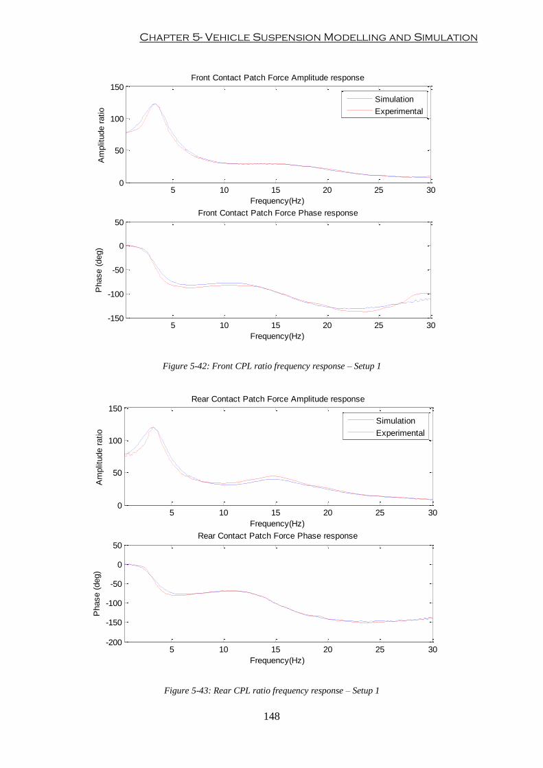
Chapter 5- Vehicle Suspension Modelling and Simulation
148
Figure 5-42: Front CPL ratio frequency response – Setup 1
Figure 5-43: Rear CPL ratio frequency response – Setup 1
5 10 15 20 25 300
50
100
150Front Contact Patch Force Amplitude response
Frequency(Hz)
Am
plit
ude r
atio
Simulation
Experimental
5 10 15 20 25 30-150
-100
-50
0
50Front Contact Patch Force Phase response
Frequency(Hz)
Phase (
deg)
5 10 15 20 25 300
50
100
150Rear Contact Patch Force Amplitude response
Frequency(Hz)
Am
plit
ude r
atio
Simulation
Experimental
5 10 15 20 25 30-200
-150
-100
-50
0
50Rear Contact Patch Force Phase response
Frequency(Hz)
Phase (
deg)
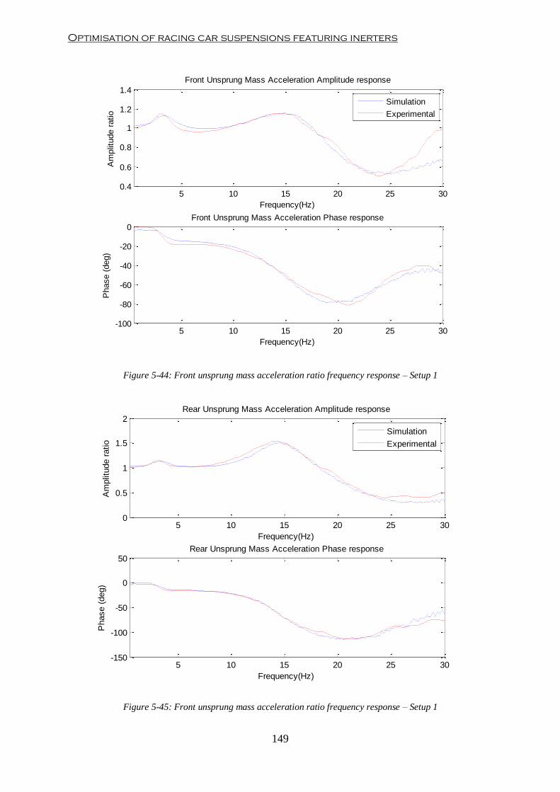
Optimisation of racing car suspensions featuring inerters
149
Figure 5-44: Front unsprung mass acceleration ratio frequency response – Setup 1
Figure 5-45: Front unsprung mass acceleration ratio frequency response – Setup 1
5 10 15 20 25 300.4
0.6
0.8
1
1.2
1.4
Front Unsprung Mass Acceleration Amplitude response
Frequency(Hz)
Am
plit
ude r
atio
Simulation
Experimental
5 10 15 20 25 30-100
-80
-60
-40
-20
0Front Unsprung Mass Acceleration Phase response
Frequency(Hz)
Phase (
deg)
5 10 15 20 25 300
0.5
1
1.5
2Rear Unsprung Mass Acceleration Amplitude response
Frequency(Hz)
Am
plit
ude r
atio
Simulation
Experimental
5 10 15 20 25 30-150
-100
-50
0
50Rear Unsprung Mass Acceleration Phase response
Frequency(Hz)
Phase (
deg)
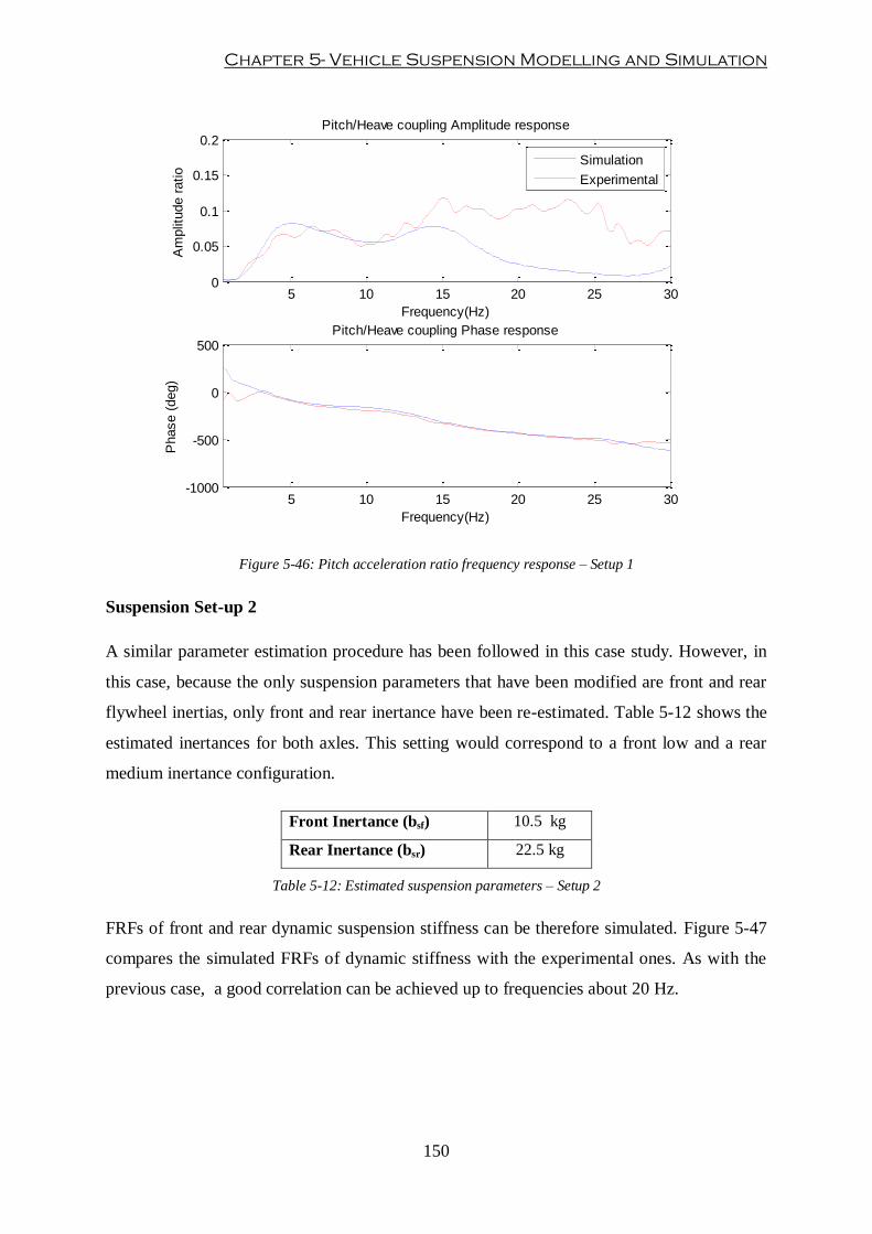
Chapter 5- Vehicle Suspension Modelling and Simulation
150
Figure 5-46: Pitch acceleration ratio frequency response – Setup 1
Suspension Set-up 2
A similar parameter estimation procedure has been followed in this case study. However, in
this case, because the only suspension parameters that have been modified are front and rear
flywheel inertias, only front and rear inertance have been re-estimated. Table 5-12 shows the
estimated inertances for both axles. This setting would correspond to a front low and a rear
medium inertance configuration.
Front Inertance (bsf) 10.5 kg
Rear Inertance (bsr) 22.5 kg
Table 5-12: Estimated suspension parameters – Setup 2
FRFs of front and rear dynamic suspension stiffness can be therefore simulated. Figure 5-47
compares the simulated FRFs of dynamic stiffness with the experimental ones. As with the
previous case, a good correlation can be achieved up to frequencies about 20 Hz.
5 10 15 20 25 300
0.05
0.1
0.15
0.2Pitch/Heave coupling Amplitude response
Frequency(Hz)
Am
plit
ude r
atio
Simulation
Experimental
5 10 15 20 25 30-1000
-500
0
500Pitch/Heave coupling Phase response
Frequency(Hz)
Phase (
deg)

Optimisation of racing car suspensions featuring inerters
151
Figure 5-47: Dynamic stiffness frequency response Setup 2: front (upper) and rear (lower)
Figure 5-48 to Figure 5-54 compare simulated dynamic responses with directly measured
magnitudes, i.e. body acceleration, hub acceleration and CPL at both ends as well as
pitch/heave interaction. Results show a high level of agreement between experimental data
and simulation.
5 10 15 20 25 300
2
4
6x 10
5 Front dynamic suspension stiffness Amplitude response
Frequency(Hz)
Dynam
ic S
tiff
ness (
N/m
)
Simulation
Experimental
5 10 15 20 25 30
0
1
2
x 106 Rear dynamic suspension stiffness Amplitude response
Frequency(Hz)
Dynam
ic S
tiff
ness (
N/m
)
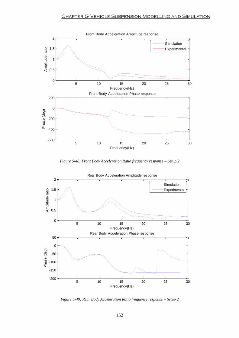
Chapter 5- Vehicle Suspension Modelling and Simulation
152
Figure 5-48: Front Body Acceleration Ratio frequency response – Setup 2
Figure 5-49: Rear Body Acceleration Ratio frequency response – Setup 2
5 10 15 20 25 300
0.5
1
1.5
2Front Body Acceleration Amplitude response
Frequency(Hz)
Am
plit
ude r
atio
Simulation
Experimental
5 10 15 20 25 30-600
-400
-200
0
200Front Body Acceleration Phase response
Frequency(Hz)
Phase (
deg)
5 10 15 20 25 300
0.5
1
1.5
2Rear Body Acceleration Amplitude response
Frequency(Hz)
Am
plit
ude r
atio
Simulation
Experimental
5 10 15 20 25 30-200
-150
-100
-50
0
50Rear Body Acceleration Phase response
Frequency(Hz)
Phase (
deg)

Optimisation of racing car suspensions featuring inerters
153
Figure 5-50: Front CPL ratio frequency response – Setup 2
Figure 5-51: Rear CPL ratio frequency response – Setup 2
5 10 15 20 25 300
50
100
150Front Contact Patch Force Amplitude response
Frequency(Hz)
Am
plit
ude r
atio
Simulation
Experimental
5 10 15 20 25 30-150
-100
-50
0
50Front Contact Patch Force Phase response
Frequency(Hz)
Phase (
deg)
5 10 15 20 25 300
50
100
150Rear Contact Patch Force Amplitude response
Frequency(Hz)
Am
plit
ude r
atio
Simulation
Experimental
5 10 15 20 25 30-200
-150
-100
-50
0
50Rear Contact Patch Force Phase response
Frequency(Hz)
Phase (
deg)

Chapter 5- Vehicle Suspension Modelling and Simulation
154
Figure 5-52: Front unsprung mass acceleration ratio frequency response – Setup 2
Figure 5-53: Rear unsprung mass acceleration ratio frequency response – Setup 2
5 10 15 20 25 300.4
0.6
0.8
1
1.2
1.4
Front Unsprung Mass Acceleration Amplitude response
Frequency(Hz)
Am
plit
ude r
atio
Simulation
Experimental
5 10 15 20 25 30-100
-50
0
50Front Unsprung Mass Acceleration Phase response
Frequency(Hz)
Phase (
deg)
5 10 15 20 25 300
0.5
1
1.5
2
2.5Rear Unsprung Mass Acceleration Amplitude response
Frequency(Hz)
Am
plit
ude r
atio
Simulation
Experimental
5 10 15 20 25 30-150
-100
-50
0
50Rear Unsprung Mass Acceleration Phase response
Frequency(Hz)
Phase (
deg)

Optimisation of racing car suspensions featuring inerters
155
Figure 5-54: Pitch acceleration ratio frequency response – Setup 2
Suspension Set-up 3
Flywheel inertia settings have been increased in this setup to validate the performance of the
vehicle model under mid inertance characteristics. In this case, the flywheel of both front and
rear inerters has been fitted with a 6-mm FWM plus a 4-mm steel disk. New inertance linear
rates have been estimated leaving the rest of suspension parameters unchanged. Inertance
values are summarised in Table 5-13.
Front Inertance (bsf) 16.5 kg
Rear Inertance (bsr) 31.5 kg
Table 5-13: Estimated suspension parameters – Setup 3
Figure 5-55 shows a comparison between experimental and estimated dynamic suspension
stiffness responses for front and rear axles.
5 10 15 20 25 300
0.2
0.4
0.6
0.8Pitch/Heave coupling Amplitude response
Frequency(Hz)
Am
plit
ude r
atio
Simulation
Experimental
5 10 15 20 25 30-1000
-500
0
500Pitch/Heave coupling Phase response
Frequency(Hz)
Phase (
deg)

Chapter 5- Vehicle Suspension Modelling and Simulation
156
Figure 5-55: Dynamic stiffness frequency response Setup 3: front (upper) and rear (lower)
The model is run again and results are compared against experimental data. Figure 5-56 to
Figure 5-62 show the dynamic response of the vehicle measured magnitudes with this new
suspension setting in the frequency domain. Although simulated body acceleration amplitude
ratio responses at both axles are slightly overestimated, especially in the region around the
hub mode, the model can predict the dynamic behaviour of the system with good levels of
accuracy.
5 10 15 20 25 300
2
4
6
8x 10
5 Front dynamic suspension stiffness Amplitude response
Frequency(Hz)
Dynam
ic S
tiff
ness (
N/m
)
Simulation
Experimental
5 10 15 20 25 300
1
2
3x 10
6 Rear dynamic suspension stiffness Amplitude response
Frequency(Hz)
Dynam
ic S
tiff
ness (
N/m
)
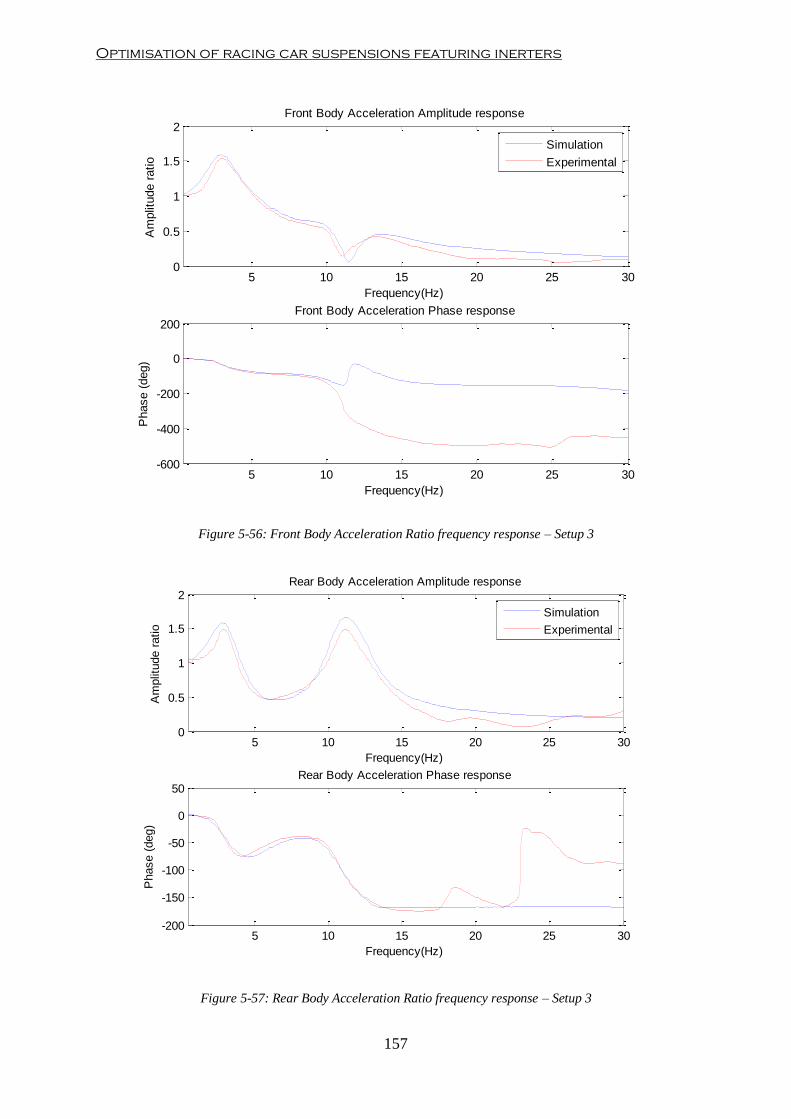
Optimisation of racing car suspensions featuring inerters
157
Figure 5-56: Front Body Acceleration Ratio frequency response – Setup 3
Figure 5-57: Rear Body Acceleration Ratio frequency response – Setup 3
5 10 15 20 25 300
0.5
1
1.5
2Front Body Acceleration Amplitude response
Frequency(Hz)
Am
plit
ude r
atio
Simulation
Experimental
5 10 15 20 25 30-600
-400
-200
0
200Front Body Acceleration Phase response
Frequency(Hz)
Phase (
deg)
5 10 15 20 25 300
0.5
1
1.5
2Rear Body Acceleration Amplitude response
Frequency(Hz)
Am
plit
ude r
atio
Simulation
Experimental
5 10 15 20 25 30-200
-150
-100
-50
0
50Rear Body Acceleration Phase response
Frequency(Hz)
Phase (
deg)
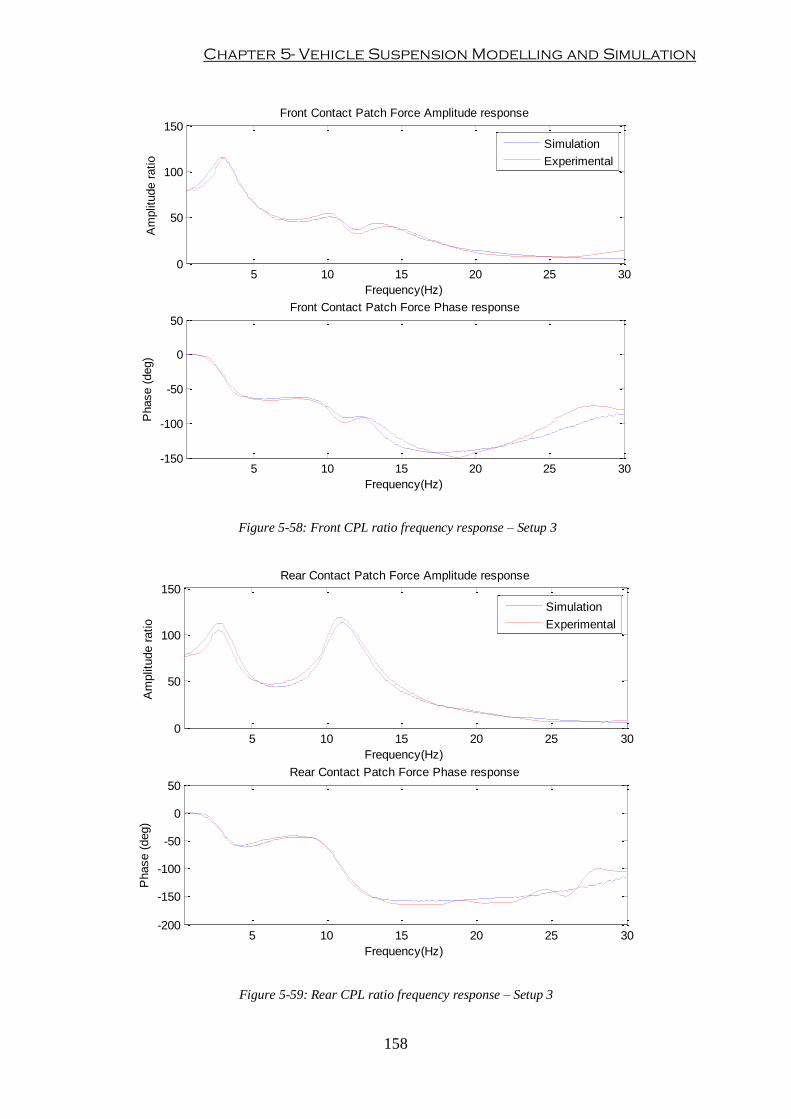
Chapter 5- Vehicle Suspension Modelling and Simulation
158
Figure 5-58: Front CPL ratio frequency response – Setup 3
Figure 5-59: Rear CPL ratio frequency response – Setup 3
5 10 15 20 25 300
50
100
150Front Contact Patch Force Amplitude response
Frequency(Hz)
Am
plit
ude r
atio
Simulation
Experimental
5 10 15 20 25 30-150
-100
-50
0
50Front Contact Patch Force Phase response
Frequency(Hz)
Phase (
deg)
5 10 15 20 25 300
50
100
150Rear Contact Patch Force Amplitude response
Frequency(Hz)
Am
plit
ude r
atio
Simulation
Experimental
5 10 15 20 25 30-200
-150
-100
-50
0
50Rear Contact Patch Force Phase response
Frequency(Hz)
Phase (
deg)

Optimisation of racing car suspensions featuring inerters
159
Figure 5-60: Front unsprung mass acceleration ratio frequency response – Setup 3
Figure 5-61: Rear unsprung mass acceleration ratio frequency response – Setup 3
5 10 15 20 25 300
0.5
1
1.5
2Front Unsprung Mass Acceleration Amplitude response
Frequency(Hz)
Am
plit
ude r
atio
Simulation
Experimental
5 10 15 20 25 30-100
-50
0
50Front Unsprung Mass Acceleration Phase response
Frequency(Hz)
Phase (
deg)
5 10 15 20 25 300
1
2
3Rear Unsprung Mass Acceleration Amplitude response
Frequency(Hz)
Am
plit
ude r
atio
Simulation
Experimental
5 10 15 20 25 30-200
-150
-100
-50
0
50Rear Unsprung Mass Acceleration Phase response
Frequency(Hz)
Phase (
deg)
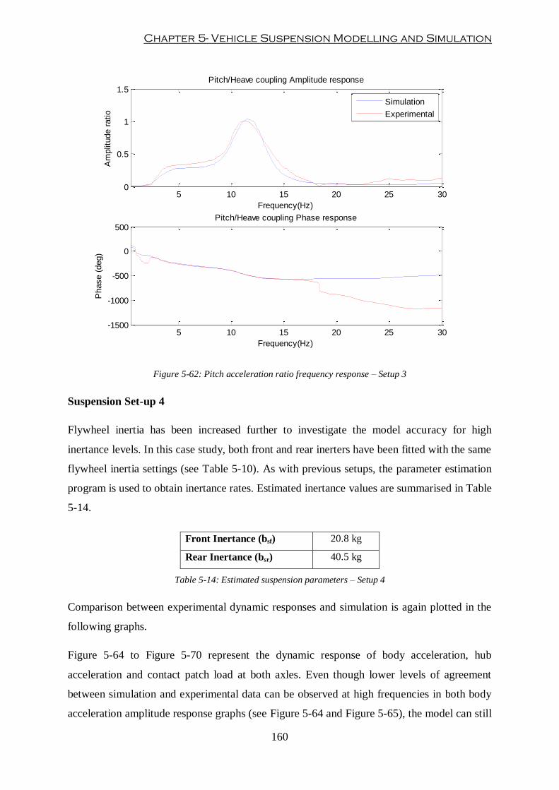
Chapter 5- Vehicle Suspension Modelling and Simulation
160
Figure 5-62: Pitch acceleration ratio frequency response – Setup 3
Suspension Set-up 4
Flywheel inertia has been increased further to investigate the model accuracy for high
inertance levels. In this case study, both front and rear inerters have been fitted with the same
flywheel inertia settings (see Table 5-10). As with previous setups, the parameter estimation
program is used to obtain inertance rates. Estimated inertance values are summarised in Table
5-14.
Front Inertance (bsf) 20.8 kg
Rear Inertance (bsr) 40.5 kg
Table 5-14: Estimated suspension parameters – Setup 4
Comparison between experimental dynamic responses and simulation is again plotted in the
following graphs.
Figure 5-64 to Figure 5-70 represent the dynamic response of body acceleration, hub
acceleration and contact patch load at both axles. Even though lower levels of agreement
between simulation and experimental data can be observed at high frequencies in both body
acceleration amplitude response graphs (see Figure 5-64 and Figure 5-65), the model can still
5 10 15 20 25 300
0.5
1
1.5Pitch/Heave coupling Amplitude response
Frequency(Hz)
Am
plit
ude r
atio
Simulation
Experimental
5 10 15 20 25 30-1500
-1000
-500
0
500Pitch/Heave coupling Phase response
Frequency(Hz)
Phase (
deg)

Optimisation of racing car suspensions featuring inerters
161
predict the dynamic behaviour of the actual vehicle. Moreover, the accuracy of the model in
predicting accurate contact patch load dynamic variation is high.
Figure 5-63: Dynamic stiffness frequency response Setup 4: front (upper) and rear (lower)
Figure 5-64: Front Body Acceleration Ratio frequency response – Setup 4
5 10 15 20 25 300
5
10x 10
5 Front dynamic suspension stiffness Amplitude response
Frequency(Hz)
Dynam
ic S
tiff
ness (
N/m
)
Simulation
Experimental
5 10 15 20 25 300
1
2
3
4x 10
6 Rear dynamic suspension stiffness Amplitude response
Frequency(Hz)
Dynam
ic S
tiff
ness (
N/m
)
5 10 15 20 25 300
0.5
1
1.5
2Front Body Acceleration Amplitude response
Frequency(Hz)
Am
plit
ude r
atio
Simulation
Experimental
5 10 15 20 25 30-600
-400
-200
0
200Front Body Acceleration Phase response
Frequency(Hz)
Phase (
deg)

Chapter 5- Vehicle Suspension Modelling and Simulation
162
Figure 5-65: Rear Body Acceleration Ratio frequency response – Setup 4
Figure 5-66: Front CPL ratio frequency response – Setup 4
5 10 15 20 25 300
0.5
1
1.5
2
2.5Rear Body Acceleration Amplitude response
Frequency(Hz)
Am
plit
ude r
atio
Simulation
Experimental
5 10 15 20 25 30-300
-200
-100
0
100Rear Body Acceleration Phase response
Frequency(Hz)
Phase (
deg)
5 10 15 20 25 300
50
100
150Front Contact Patch Force Amplitude response
Frequency(Hz)
Am
plit
ude r
atio
Simulation
Experimental
5 10 15 20 25 30-200
-150
-100
-50
0
50Front Contact Patch Force Phase response
Frequency(Hz)
Phase (
deg)
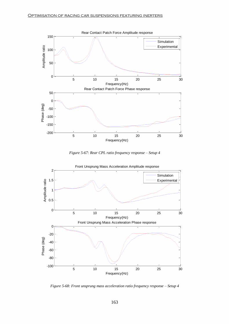
Optimisation of racing car suspensions featuring inerters
163
Figure 5-67: Rear CPL ratio frequency response – Setup 4
Figure 5-68: Front unsprung mass acceleration ratio frequency response – Setup 4
5 10 15 20 25 300
50
100
150Rear Contact Patch Force Amplitude response
Frequency(Hz)
Am
plit
ude r
atio
Simulation
Experimental
5 10 15 20 25 30-200
-150
-100
-50
0
50Rear Contact Patch Force Phase response
Frequency(Hz)
Phase (
deg)
5 10 15 20 25 300
0.5
1
1.5
2Front Unsprung Mass Acceleration Amplitude response
Frequency(Hz)
Am
plit
ude r
atio
Simulation
Experimental
5 10 15 20 25 30-100
-80
-60
-40
-20
0Front Unsprung Mass Acceleration Phase response
Frequency(Hz)
Phase (
deg)

Chapter 5- Vehicle Suspension Modelling and Simulation
164
Figure 5-69: Rear unsprung mass acceleration ratio frequency response – Setup 4
Figure 5-70: Pitch acceleration ratio frequency response – Setup 4
5 10 15 20 25 300
1
2
3
4Rear Unsprung Mass Acceleration Amplitude response
Frequency(Hz)
Am
plit
ude r
atio
Simulation
Experimental
5 10 15 20 25 30-200
-150
-100
-50
0
50Rear Unsprung Mass Acceleration Phase response
Frequency(Hz)
Phase (
deg)
5 10 15 20 25 300
0.5
1
1.5Pitch/Heave coupling Amplitude response
Frequency(Hz)
Am
plit
ude r
atio
Simulation
Experimental
5 10 15 20 25 30-1500
-1000
-500
0
500Pitch/Heave coupling Phase response
Frequency(Hz)
Phase (
deg)

Optimisation of racing car suspensions featuring inerters
165
Suspension Set-up 5
The last suspension setting corresponds to very high inertance characteristics. In this case
study, flywheel inertia has been further increased at both vehicle ends (see Table 5-10).
Inertance rates have been again estimated considering the rest of suspension values to remain
unvaried. Table 5-15 shows the inertance values estimated through the identification process.
Front Inertance (bsf) 30 kg
Rear Inertance (bsr) 56.5 kg
Table 5-15: Estimated suspension parameters – Setup 5
With the estimated front and rear inertance rates, experimental and simulated dynamic
suspension stiffness frequency responses can be compared (see Figure 5-71).
Figure 5-71: Dynamic stiffness frequency response Setup 5: front (upper) and rear (lower)
As in the previous case studies, simulation of the vehicle model has been run and compared
against experimental data from the four post rig.
Figure 5-72 to Figure 5-78 show the frequency-domain responses of both the actual vehicle
and the model. Although, bigger differences can be appreciated in the setup, especially in
body acceleration amplitude ratio responses (see Figure 5-72 and Figure 5-73) with respect to
5 10 15 20 25 300
5
10
15x 10
5 Front dynamic suspension stiffness Amplitude response
Frequency(Hz)
Dynam
ic S
tiff
ness (
N/m
)
Simulation
Experimental
5 10 15 20 25 300
2
4
6x 10
6 Rear dynamic suspension stiffness Amplitude response
Frequency(Hz)
Dynam
ic S
tiff
ness (
N/m
)
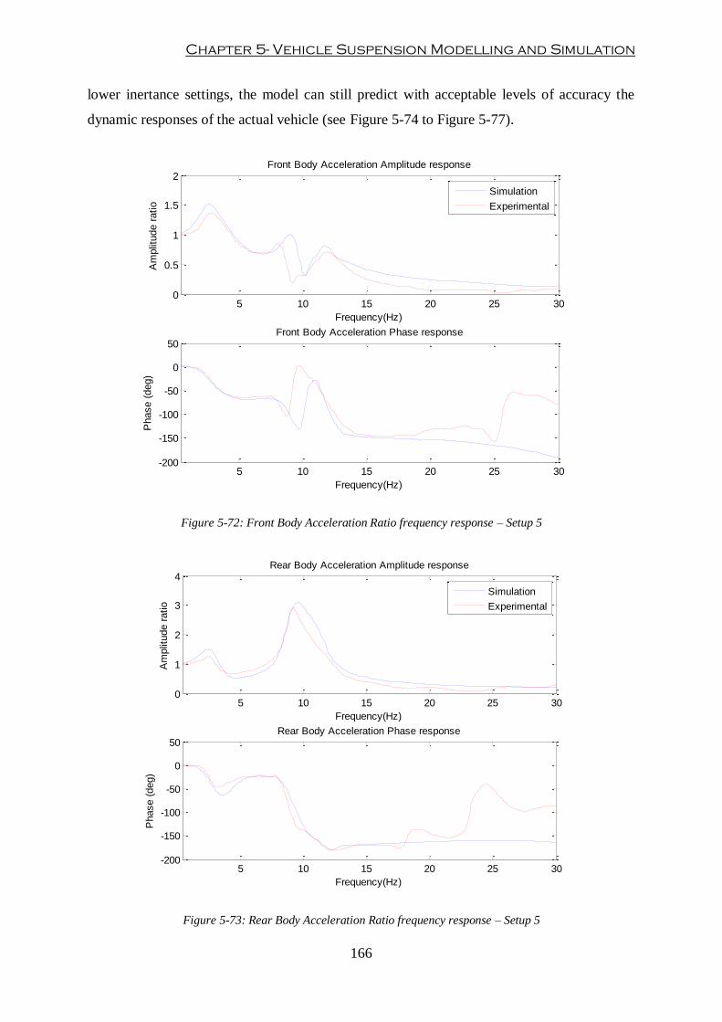
Chapter 5- Vehicle Suspension Modelling and Simulation
166
lower inertance settings, the model can still predict with acceptable levels of accuracy the
dynamic responses of the actual vehicle (see Figure 5-74 to Figure 5-77).
Figure 5-72: Front Body Acceleration Ratio frequency response – Setup 5
Figure 5-73: Rear Body Acceleration Ratio frequency response – Setup 5
5 10 15 20 25 300
0.5
1
1.5
2Front Body Acceleration Amplitude response
Frequency(Hz)
Am
plit
ude r
atio
Simulation
Experimental
5 10 15 20 25 30-200
-150
-100
-50
0
50Front Body Acceleration Phase response
Frequency(Hz)
Phase (
deg)
5 10 15 20 25 300
1
2
3
4Rear Body Acceleration Amplitude response
Frequency(Hz)
Am
plit
ude r
atio
Simulation
Experimental
5 10 15 20 25 30-200
-150
-100
-50
0
50Rear Body Acceleration Phase response
Frequency(Hz)
Phase (
deg)

Optimisation of racing car suspensions featuring inerters
167
Figure 5-74: Front CPL ratio frequency response – Setup 5
Figure 5-75: Rear CPL ratio frequency response – Setup 5
5 10 15 20 25 300
50
100
150Front Contact Patch Force Amplitude response
Frequency(Hz)
Am
plit
ude r
atio
Simulation
Experimental
5 10 15 20 25 30-200
-150
-100
-50
0
50Front Contact Patch Force Phase response
Frequency(Hz)
Phase (
deg)
5 10 15 20 25 300
50
100
150
200
250Rear Contact Patch Force Amplitude response
Frequency(Hz)
Am
plit
ude r
atio
Simulation
Experimental
5 10 15 20 25 30-200
-150
-100
-50
0
50Rear Contact Patch Force Phase response
Frequency(Hz)
Phase (
deg)

Chapter 5- Vehicle Suspension Modelling and Simulation
168
Figure 5-76: Front unsprung mass acceleration ratio frequency response – Setup 5
Figure 5-77: Rear unsprung mass acceleration ratio frequency response – Setup 5
5 10 15 20 25 300
0.5
1
1.5
2
2.5Front Unsprung Mass Acceleration Amplitude response
Frequency(Hz)
Am
plit
ude r
atio
Simulation
Experimental
5 10 15 20 25 30-100
-50
0
50Front Unsprung Mass Acceleration Phase response
Frequency(Hz)
Phase (
deg)
5 10 15 20 25 300
1
2
3
4Rear Unsprung Mass Acceleration Amplitude response
Frequency(Hz)
Am
plit
ude r
atio
Simulation
Experimental
5 10 15 20 25 30-200
-150
-100
-50
0
50Rear Unsprung Mass Acceleration Phase response
Frequency(Hz)
Phase (
deg)
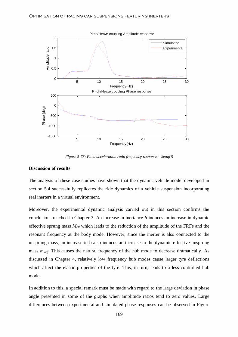
Optimisation of racing car suspensions featuring inerters
169
Figure 5-78: Pitch acceleration ratio frequency response – Setup 5
Discussion of results
The analysis of these case studies have shown that the dynamic vehicle model developed in
section 5.4 successfully replicates the ride dynamics of a vehicle suspension incorporating
real inerters in a virtual environment.
Moreover, the experimental dynamic analysis carried out in this section confirms the
conclusions reached in Chapter 3. An increase in inertance b induces an increase in dynamic
effective sprung mass Meff which leads to the reduction of the amplitude of the FRFs and the
resonant frequency at the body mode. However, since the inerter is also connected to the
unsprung mass, an increase in b also induces an increase in the dynamic effective unsprung
mass mueff. This causes the natural frequency of the hub mode to decrease dramatically. As
discussed in Chapter 4, relatively low frequency hub modes cause larger tyre deflections
which affect the elastic properties of the tyre. This, in turn, leads to a less controlled hub
mode.
In addition to this, a special remark must be made with regard to the large deviation in phase
angle presented in some of the graphs when amplitude ratios tend to zero values. Large
differences between experimental and simulated phase responses can be observed in Figure
5 10 15 20 25 300
0.5
1
1.5
2Pitch/Heave coupling Amplitude response
Frequency(Hz)
Am
plit
ude r
atio
Simulation
Experimental
5 10 15 20 25 30-1500
-1000
-500
0
500Pitch/Heave coupling Phase response
Frequency(Hz)
Phase (
deg)
Chapter 5- Vehicle Suspension Modelling and Simulation
170
5-48, Figure 5-56 and Figure 5-62. In those figures, front body acceleration phase response
jumps outside the expected phase range [-π,+π] rad at around 10-12 Hz. Although this
sudden phase change has been smoothed out by the post-processing, the actual experimental
phase experiences a phase lead similar to the predicted by the model. This is due to the way
the post-processing parameter estimation tool constructs the phase response traces from
experimental time-domain data (red traces). In the version of the post-processing tool
developed by Bennett (2012) used in this thesis, the phase response between output and input
signals is calculated from the difference in time at each peak for a given frequency. For low
output signal amplitudes (typically less than a 10% of the amplitude of input signal), the
noise found in the physical signal could alter peaks identified by the software for a given time
period. This causes the miscalculation of phase response for low amplitude ratios in Figure
5-48, Figure 5-56 and Figure 5-62. A confirmation of this behaviour can be noticed in Figure
5-72. In this case, because the amplitude ratio of the front body acceleration is higher than in
previous case, the parameter estimation program has succeeded in producing the actual phase
response. Similar phase response discontinuities can be observed in pitch acceleration FRFs
due to low amplitude ratios.
5.5.2. Analysis of model predictability via suspension optimisation
The main goal of computer simulation is to create virtual models that can be used for
analysing the dynamic behaviour of a specific system without the requirement of physical
system. Furthermore, if the computer model has been fully validated, then it could be used for
virtual optimisation. Although, Chapter 7 covers an extensive discussion on suspension
optimisation, a simple single-objective optimisation case study has been analysed in this
section. In this way, the predictive capabilities of the model for suspension optimisation can
be validated.
In this section, two case studies have been analysed separately:
Suspension optimisation of a mechanical grip cost function J1 defined as the algebraic
sum of the root-mean-square (RMS) of the amplitude ratio of the FRF of the front
dynamic CPL and rear dynamic CPL .

Optimisation of racing car suspensions featuring inerters
171
Suspension optimisation of an aerodynamic grip cost function J2: defined as the
algebraic sum of the RMS of the amplitude of the FRF of front ride height
and rear ride height .
For each case, a set of suspension parameters that minimises the objective function J was
obtained using the virtual suspension model without (S1) and with inerters (S2). A detailed
discussion of the selection of the suspension parameters that must compose the optimisation
search space will be provided in Chapter 7. In this section, front and rear damper and inerter
characteristics were used to set the optimisation search space. Table 5-16 shows the limits of
the search space selected for these case studies. Note that, for the case of a suspension
without inerters, the search space was only composed by front and rear damper
characteristics.
Min. value Max. value
Damper rate (Ns/m) 700 3500
Inerter rate (kg) 0 100
Table 5-16: Design space range – Suspension optimisation validation
According to the material reviewed in Chapter 2, a SQP algorithm was selected to perform
the optimisation process due to its strong local-convergence towards a single optimal
solution. This optimisation solver has been set making use of the built-in Matlab function for
nonlinear constrained optimisation fmincon (The MathWorks Inc., 2010).
Once optimised suspension settings were obtained, these results were then used to set the
suspension of the physical test vehicle. Experimental tests for each case were run and
experimental values for each objective function J were calculated from the FRFs of the
experimental data according to equations (5.9) and (5.10).
Mechanical grip optimisation
Table 5-17 shows the set of suspension parameters that minimises objective function J1 in the
virtual environment for both suspension configurations.
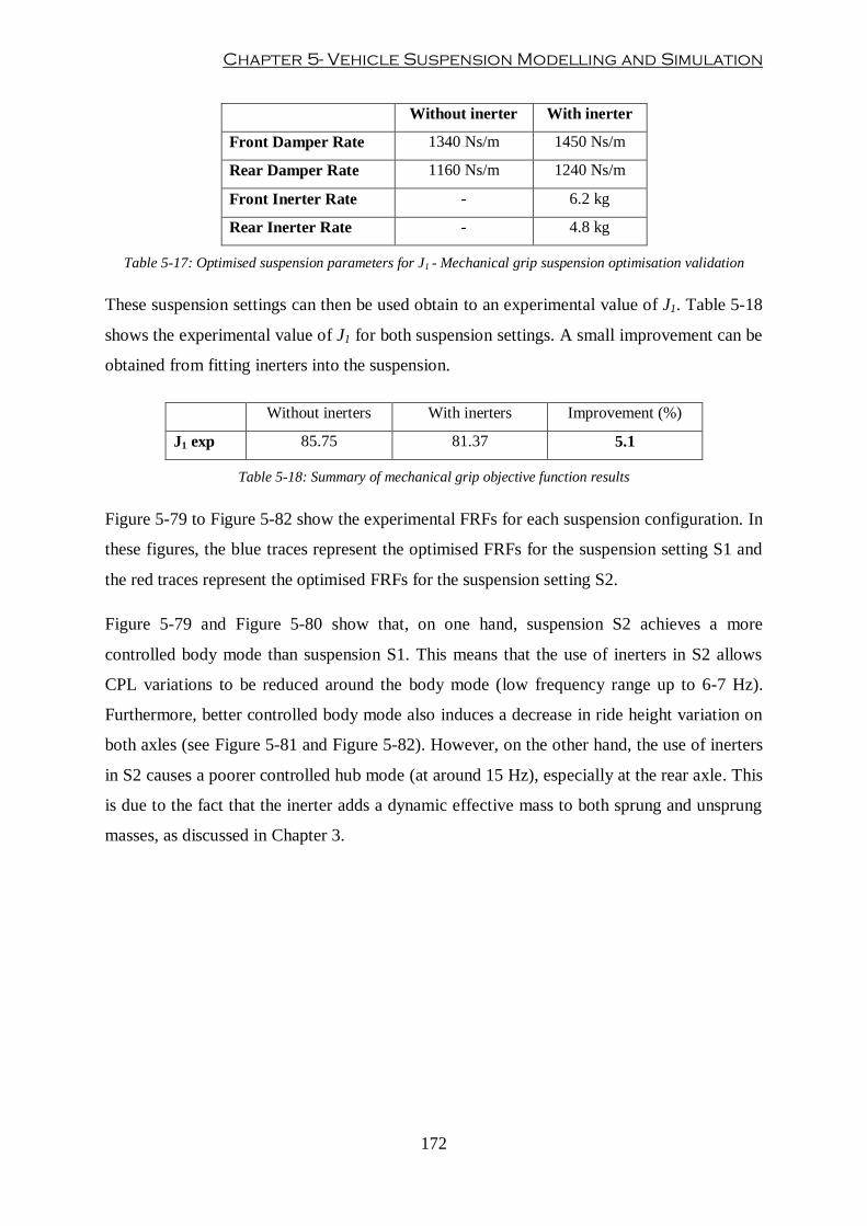
Chapter 5- Vehicle Suspension Modelling and Simulation
172
Without inerter With inerter
Front Damper Rate 1340 Ns/m 1450 Ns/m
Rear Damper Rate 1160 Ns/m 1240 Ns/m
Front Inerter Rate - 6.2 kg
Rear Inerter Rate - 4.8 kg
Table 5-17: Optimised suspension parameters for J1 - Mechanical grip suspension optimisation validation
These suspension settings can then be used obtain to an experimental value of J1. Table 5-18
shows the experimental value of J1 for both suspension settings. A small improvement can be
obtained from fitting inerters into the suspension.
Without inerters With inerters Improvement (%)
J1 exp 85.75 81.37 5.1
Table 5-18: Summary of mechanical grip objective function results
Figure 5-79 to Figure 5-82 show the experimental FRFs for each suspension configuration. In
these figures, the blue traces represent the optimised FRFs for the suspension setting S1 and
the red traces represent the optimised FRFs for the suspension setting S2.
Figure 5-79 and Figure 5-80 show that, on one hand, suspension S2 achieves a more
controlled body mode than suspension S1. This means that the use of inerters in S2 allows
CPL variations to be reduced around the body mode (low frequency range up to 6-7 Hz).
Furthermore, better controlled body mode also induces a decrease in ride height variation on
both axles (see Figure 5-81 and Figure 5-82). However, on the other hand, the use of inerters
in S2 causes a poorer controlled hub mode (at around 15 Hz), especially at the rear axle. This
is due to the fact that the inerter adds a dynamic effective mass to both sprung and unsprung
masses, as discussed in Chapter 3.

Optimisation of racing car suspensions featuring inerters
173
Figure 5-79: Front CPL response – Mechanical grip optimisation
Figure 5-80: Rear CPL response – Mechanical grip optimisation
5 10 15 20 25 300
50
100
150Force Amplitude Ratio Compasison
Frequency (Hz)
Am
plit
ude R
atio
Part1 RUN 3 Heave
Part1 RUN 5 Heave
5 10 15 20 25 30-150
-100
-50
0
50Contact Force Phase Comparison
Frequency (Hz)
Phase (
Degs)
Part1 RUN 3 Heave
Part1 RUN 5 Heave
5 10 15 20 25 300
50
100
150Force Amplitude Ratio Compasison
Frequency (Hz)
Am
plit
ude R
atio
Part1 RUN 3 Heave
Part1 RUN 5 Heave
5 10 15 20 25 30-200
-100
0
100Contact Force Phase Comparison
Frequency (Hz)
Phase (
Degs)
Part1 RUN 3 Heave
Part1 RUN 5 Heave
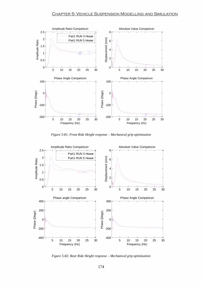
Chapter 5- Vehicle Suspension Modelling and Simulation
174
Figure 5-81: Front Ride Height response – Mechanical grip optimisation
Figure 5-82: Rear Ride Height response – Mechanical grip optimisation
5 10 15 20 25 300
0.5
1
1.5
2
2.5Amplitude Ratio Comparison
Am
plit
ude R
atio
Part1 RUN 3 Heave
Part1 RUN 5 Heave
5 10 15 20 25 30-200
-100
0
100Phase Angle Comparison
Frequency (Hz)
Phase (
Degs)
5 10 15 20 25 300
2
4
6
8Absolute Value Comparison
Dis
pla
cem
ent
(mm
)
5 10 15 20 25 30-200
-100
0
100Phase Angle Comparison
Frequency (Hz)
Phase (
Degs)
5 10 15 20 25 300
0.5
1
1.5
2
2.5Amplitude Ratio Comparison
Am
plit
ude R
atio
Part1 RUN 3 Heave
Part1 RUN 5 Heave
5 10 15 20 25 30-400
-200
0
200
400Phase angle Comparison
Frequency (Hz)
Phase (
Degs)
5 10 15 20 25 300
2
4
6
8Absolute Value Comparison
Dis
pla
cem
ent
(mm
)
5 10 15 20 25 30-400
-200
0
200
400Phase Angle Comparison
Frequency (Hz)
Phase (
Degs)
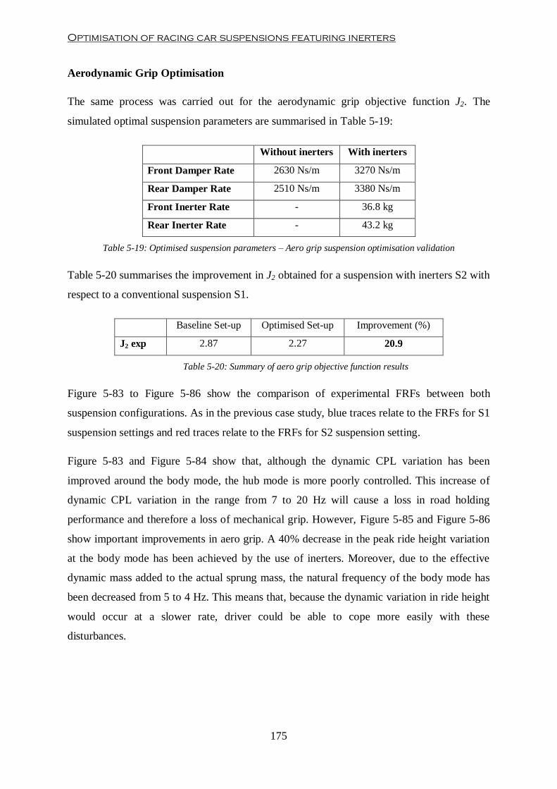
Optimisation of racing car suspensions featuring inerters
175
Aerodynamic Grip Optimisation
The same process was carried out for the aerodynamic grip objective function J2. The
simulated optimal suspension parameters are summarised in Table 5-19:
Without inerters With inerters
Front Damper Rate 2630 Ns/m 3270 Ns/m
Rear Damper Rate 2510 Ns/m 3380 Ns/m
Front Inerter Rate - 36.8 kg
Rear Inerter Rate - 43.2 kg
Table 5-19: Optimised suspension parameters – Aero grip suspension optimisation validation
Table 5-20 summarises the improvement in J2 obtained for a suspension with inerters S2 with
respect to a conventional suspension S1.
Baseline Set-up Optimised Set-up Improvement (%)
J2 exp 2.87 2.27 20.9
Table 5-20: Summary of aero grip objective function results
Figure 5-83 to Figure 5-86 show the comparison of experimental FRFs between both
suspension configurations. As in the previous case study, blue traces relate to the FRFs for S1
suspension settings and red traces relate to the FRFs for S2 suspension setting.
Figure 5-83 and Figure 5-84 show that, although the dynamic CPL variation has been
improved around the body mode, the hub mode is more poorly controlled. This increase of
dynamic CPL variation in the range from 7 to 20 Hz will cause a loss in road holding
performance and therefore a loss of mechanical grip. However, Figure 5-85 and Figure 5-86
show important improvements in aero grip. A 40% decrease in the peak ride height variation
at the body mode has been achieved by the use of inerters. Moreover, due to the effective
dynamic mass added to the actual sprung mass, the natural frequency of the body mode has
been decreased from 5 to 4 Hz. This means that, because the dynamic variation in ride height
would occur at a slower rate, driver could be able to cope more easily with these
disturbances.
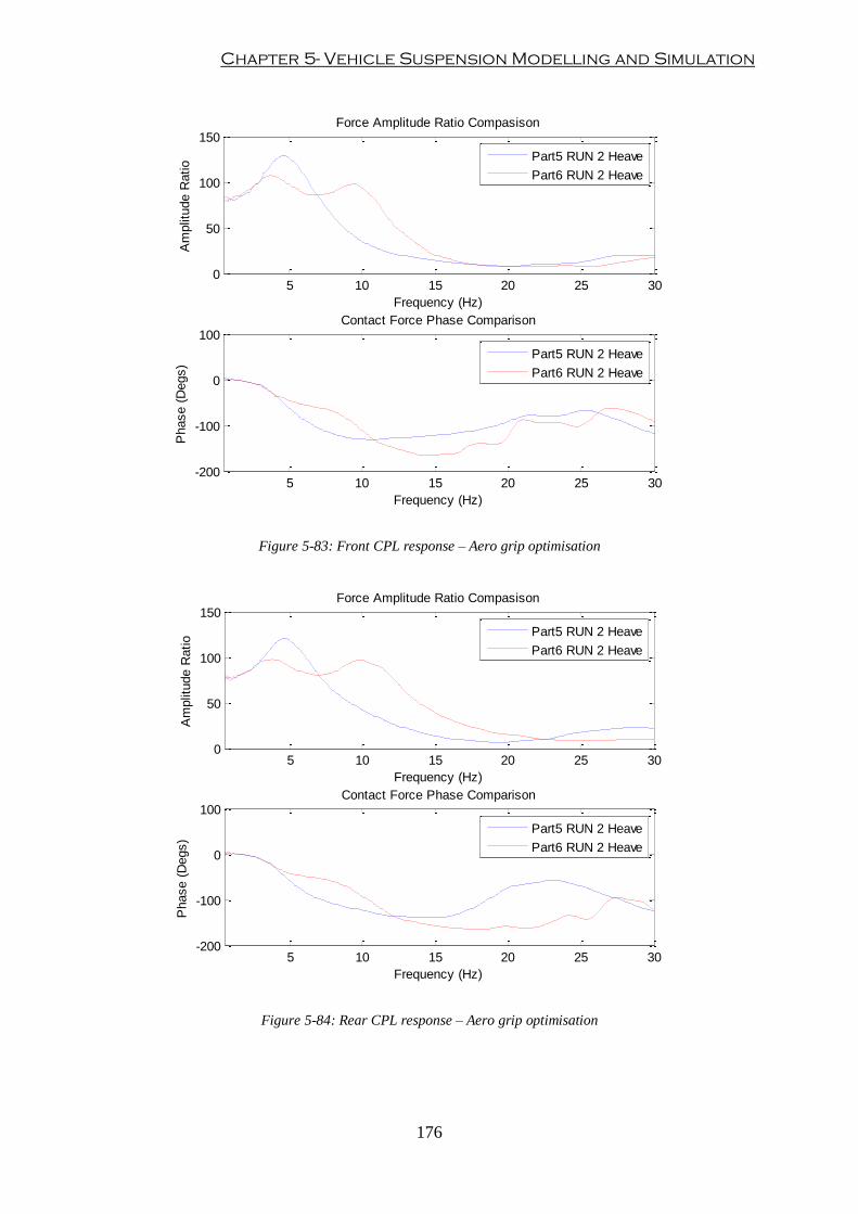
Chapter 5- Vehicle Suspension Modelling and Simulation
176
Figure 5-83: Front CPL response – Aero grip optimisation
Figure 5-84: Rear CPL response – Aero grip optimisation
5 10 15 20 25 300
50
100
150Force Amplitude Ratio Compasison
Frequency (Hz)
Am
plit
ude R
atio
Part5 RUN 2 Heave
Part6 RUN 2 Heave
5 10 15 20 25 30-200
-100
0
100Contact Force Phase Comparison
Frequency (Hz)
Phase (
Degs)
Part5 RUN 2 Heave
Part6 RUN 2 Heave
5 10 15 20 25 300
50
100
150Force Amplitude Ratio Compasison
Frequency (Hz)
Am
plit
ude R
atio
Part5 RUN 2 Heave
Part6 RUN 2 Heave
5 10 15 20 25 30-200
-100
0
100Contact Force Phase Comparison
Frequency (Hz)
Phase (
Degs)
Part5 RUN 2 Heave
Part6 RUN 2 Heave

Optimisation of racing car suspensions featuring inerters
177
Figure 5-85: Front Ride Height response – Aero grip optimisation
Figure 5-86: Rear Ride Height response – Aero grip optimisation
5 10 15 20 25 300
0.5
1
1.5
2Amplitude Ratio Comparison
Am
plit
ude R
atio
5 10 15 20 25 30-300
-200
-100
0
100
200Phase Angle Comparison
Frequency (Hz)
Phase (
Degs)
5 10 15 20 25 300
1
2
3
4
5Absolute Value Comparison
Dis
pla
cem
ent
(mm
)
Part5 RUN 2 Heave
Part6 RUN 2 Heave
5 10 15 20 25 30-300
-200
-100
0
100
200Phase Angle Comparison
Frequency (Hz)
Phase (
Degs)
5 10 15 20 25 300
0.5
1
1.5
2Amplitude Ratio Comparison
Am
plit
ude R
atio
5 10 15 20 25 300
100
200
300
400
500Phase angle Comparison
Frequency (Hz)
Phase (
Degs)
5 10 15 20 25 300
1
2
3
4Absolute Value Comparison
Dis
pla
cem
ent
(mm
)
Part5 RUN 2 Heave
Part6 RUN 2 Heave
5 10 15 20 25 300
100
200
300
400
500Phase Angle Comparison
Frequency (Hz)
Phase (
Degs)
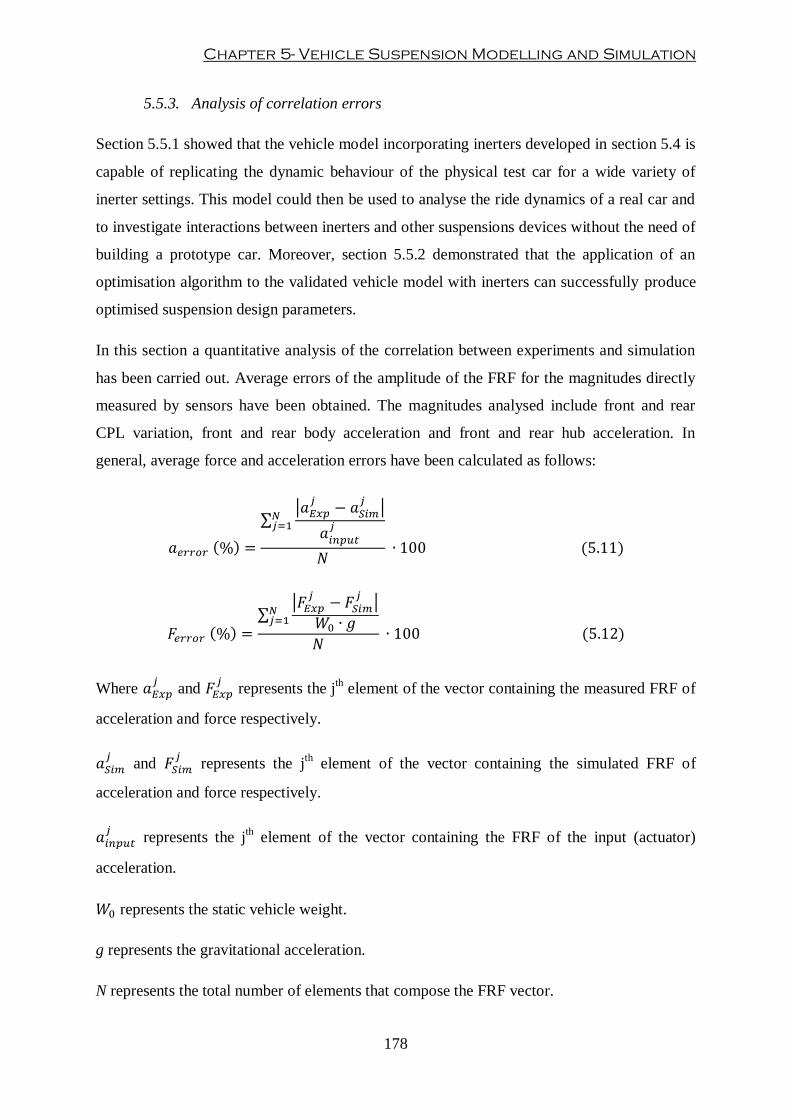
Chapter 5- Vehicle Suspension Modelling and Simulation
178
5.5.3. Analysis of correlation errors
Section 5.5.1 showed that the vehicle model incorporating inerters developed in section 5.4 is
capable of replicating the dynamic behaviour of the physical test car for a wide variety of
inerter settings. This model could then be used to analyse the ride dynamics of a real car and
to investigate interactions between inerters and other suspensions devices without the need of
building a prototype car. Moreover, section 5.5.2 demonstrated that the application of an
optimisation algorithm to the validated vehicle model with inerters can successfully produce
optimised suspension design parameters.
In this section a quantitative analysis of the correlation between experiments and simulation
has been carried out. Average errors of the amplitude of the FRF for the magnitudes directly
measured by sensors have been obtained. The magnitudes analysed include front and rear
CPL variation, front and rear body acceleration and front and rear hub acceleration. In
general, average force and acceleration errors have been calculated as follows:
Where
and
represents the jth element of the vector containing the measured FRF of
acceleration and force respectively.
and
represents the jth
element of the vector containing the simulated FRF of
acceleration and force respectively.
represents the jth element of the vector containing the FRF of the input (actuator)
acceleration.
represents the static vehicle weight.
g represents the gravitational acceleration.
N represents the total number of elements that compose the FRF vector.

Optimisation of racing car suspensions featuring inerters
179
Table 5-21 summarises the average error of all the measured magnitudes for the five
suspension settings analysed in section 5.5.1.
Setup 1 Setup 2 Setup 3 Setup 4 Setup 5
Front Body Acc 7.1% 5.3% 5.9% 7.5% 8.5%
Rear Body Acc 7.3% 10.0% 10.8% 12.5% 15.7%
Front CPL 0.7% 1.3% 2.3% 3.3% 3.5%
Rear CPL 1.6% 1.6% 2.4% 2.4% 2.2%
Front Hub Acc 4.7% 6.0% 13.6% 16.4% 18.9%
Rear Hub Acc 4.5% 6.6% 7.5% 9.0% 11.2%
Table 5-21: Summary of validation errors
From the results above, it can be observed that the level of agreement between experimental
and simulated is high. Dynamic contact patch load responses are the most accurate
measurements with a maximum averaged error of 3.5%. Body acceleration frequency
responses present also good levels of accuracy. As it can be observed from body acceleration
dynamic response figures (see section 5.5.1), the largest deviation between simulation and
experimental data was produced by an overestimation of amplitude at around the hub mode.
Since this thesis focuses on performance of a race car rather than comfort, body acceleration
FRF has been used to produce the ride height FRFs. According to this, it has been analysed
that, even in the worst case scenario (rear body acceleration in setup 5), the difference
induced in ride height would be less than 0.3 mm for a 25-mm amplitude road input. Hub
acceleration dynamic response presents the highest accuracy errors of all measured
magnitudes. From figures shown in section 5.5.1, the largest errors are produced at high
frequencies (from 20 Hz onwards). In this high frequency bandwidth, the impact of unsprung
mass acceleration in the ride dynamics of the vehicle is quite low since the hub mode occurs
at lower frequencies when the suspension incorporates inerters. According to this, a new
analysis of the average relative hub acceleration errors has been carried out neglecting the 20-
30 Hz frequency band. Results show that the level of accuracy is much higher within the
frequency region where hub accelerations have an impact in the overall ride dynamics of the
vehicle (see Table 5-22).

Chapter 5- Vehicle Suspension Modelling and Simulation
180
Setup 1 Setup 2 Setup 3 Setup 4 Setup 5
Front Hub Acc 5.3% 2.4% 6.5% 7.8% 8.8%
Rear Hub Acc 4.8% 3.4% 4.1% 6.2% 8.9%
Table 5-22: Hub acceleration average errors – Frequency range 0.5-20 Hz
Furthermore, there is progressive increase of the prediction error as the inertance
characteristic increases. This is due to a number of reasons: firstly, the inerter has been
modelled as a linear inertance characteristic that include linear parasitic effects such as inerter
compliance and friction. These parasitic effects are, however, rarely linear. For low inertance
settings, these parasitic effects have a marginal effect on the dynamic response of the
suspension, thus the model could be approximated to a linear ideal inerter. As inertance
values increase, inerter parasitic effects take over and their impact in the performance of the
suspension is much more noticeable (see Figure 5-22). Under these conditions, deviations
from linear behaviour will cause a source of error. Nonlinear models, however, do not allow
the construction of suspension model via a SISO transfer function. Furthermore, the use of
nonlinear models would increase parameter estimation complexity and simulation time.
Secondly, tyre model plays an important role in model accuracy. Section 5.4.2 demonstrated
that the use of linear tyre elastic properties would be insufficient if high accuracy is required.
Alternatively, a nonlinear exponential model has been proposed to account for the interaction
between tyre elastic characteristics (i.e. tyre stiffness and damping) and tyre dynamic
deflection. Even though this model is a better representation of the behaviour of the physical
tyre, it was observed that the front tyres present a hysteretic behaviour, especially as inertance
settings increased. Figure 5-87 shows the differences in front and rear tyre behaviour between
a low and high inertance setting. Rear tyres present a mainly exponential-like elastic
characteristic for both inertance settings. However, the difference in tyre stiffness
characteristic at the front axle is much larger. Although an exponential characteristic can still
be appreciated, hysteresis is quite large with a heavy inerter setting. Tyres are very complex
and highly nonlinear systems and a detailed study and analysis of nonlinear tyre behaviour is
out of the scope of the present research work. Causes of this hysteretic behaviour could come
from complex interactions between tyre rubber, tyre carcass, tyre sidewall construction and
compressed air at high tyre deflections. It must be noted that, for very low tyre deflections,
the estimation of tyre stiffness is not accurate, due to the high noise-to-signal ratio (close to
1). This explains the non-uniqueness of tyre stiffness estimation for a given tyre deflection.
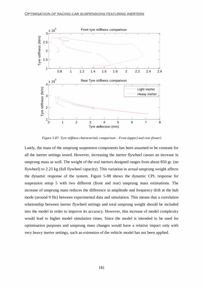
Optimisation of racing car suspensions featuring inerters
181
Figure 5-87: Tyre stiffness characteristic comparison – Front (upper) and rear (lower)
Lastly, the mass of the unsprung suspension components has been assumed to be constant for
all the inerter settings tested. However, increasing the inerter flywheel causes an increase in
unsprung mass as well. The weight of the real inerters designed ranges from about 850 gr. (no
flywheel) to 2.25 kg (full flywheel capacity). This variation in actual unsprung weight affects
the dynamic response of the system. Figure 5-88 shows the dynamic CPL response for
suspension setup 5 with two different (front and rear) unsprung mass estimations. The
increase of unsprung mass reduces the difference in amplitude and frequency drift at the hub
mode (around 9 Hz) between experimental data and simulation. This means that a correlation
relationship between inerter flywheel settings and total unsprung weight should be included
into the model in order to improve its accuracy. However, this increase of model complexity
would lead to higher model simulation times. Since the model is intended to be used for
optimisation purposes and unsprung mass changes would have a relative impact only with
very heavy inerter settings, such an extension of the vehicle model has not been applied.
0.8 1 1.2 1.4 1.6 1.8 2 2.2 2.4 2.61
1.5
2
2.5
3x 10
5
Tyre
stiff
ness (
N/m
)
Front tyre stiffness comparison
0 1 2 3 4 5 6 7 81
2
3
4x 10
5
Tyre deflection (mm)
Tyre
stiff
ness (
N/m
)
Rear Tyre stiffness comparison
Light inerter
Heavy inerter
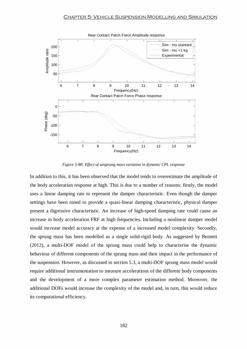
Chapter 5- Vehicle Suspension Modelling and Simulation
182
Figure 5-88: Effect of unsprung mass variation in dynamic CPL response
In addition to this, it has been observed that the model tends to overestimate the amplitude of
the body acceleration response at high. This is due to a number of reasons: firstly, the model
uses a linear damping rate to represent the damper characteristic. Even though the damper
settings have been tuned to provide a quasi-linear damping characteristic, physical damper
present a digressive characteristic. An increase of high-speed damping rate could cause an
increase in body acceleration FRF at high frequencies. Including a nonlinear damper model
would increase model accuracy at the expense of a increased model complexity. Secondly,
the sprung mass has been modelled as a single solid-rigid body. As suggested by Bennett
(2012), a multi-DOF model of the sprung mass could help to characterise the dynamic
behaviour of different components of the sprung mass and their impact in the performance of
the suspension. However, as discussed in section 5.3, a multi-DOF sprung mass model would
require additional instrumentation to measure accelerations of the different body components
and the development of a more complex parameter estimation method. Moreover, the
additional DOFs would increase the complexity of the model and, in turn, this would reduce
its computational efficiency.
6 7 8 9 10 11 12 13 14
50
100
150
200
Rear Contact Patch Force Amplitude response
Frequency(Hz)
Am
plit
ude r
atio
Sim - mu stantard
Sim - mu +1 kg
Experimental
6 7 8 9 10 11 12 13 14
-150
-100
-50
0
Rear Contact Patch Force Phase response
Frequency(Hz)
Phase (
deg)

Optimisation of racing car suspensions featuring inerters
183
In spite of these sources of errors, the model developed in this chapter is capable of
replicating a physical suspension incorporating inerters with a degree of accuracy so that the
main dynamic features of the system (i.e. natural frequencies and amplitude ratios) can be
successfully identified by this model.
Chapter 5- Vehicle Suspension Modelling and Simulation
184
5.6. Summary
In this chapter a novel vehicle model featuring inerters for the analysis and optimisation of
high performance car suspensions has been developed. Experimental data obtained from four-
post rig testing has been used to estimate all the vehicle and suspension parameters. These
parameters have then been used to simulate the vehicle model and results have been
compared against experimental FRF of the physical vehicle. Several suspension settings have
been tested in order to demonstrate the accuracy of the vehicle model over a vast range of
inerter configurations. The model has been deemed to successfully represent the dynamic
behaviour of a vehicle suspension fitted with physical inerters.
Moreover, the model developed in this chapter has been used as part of an optimisation
process. The main purpose of this study has been to evaluate the predictive capabilities of the
vehicle model applied to suspension design and optimisation. The model successfully
produced optimised suspension settings for two different performance objective functions.
The experimental analysis of the suspension incorporating inerters carried out in this chapter
showed that although increasing the inertance characteristic was beneficial for a better
controlled body mode at low frequencies, this increase in inertance would cause a
deterioration of the dynamic response at higher frequencies due to a less controlled hub
model.
A critical discussion of model accuracy has been carried out. Different sources of error
between experimental data and simulation have been identified and their impact in the
dynamic response of the vehicle has been assessed. Results show that, although potential
improvements in model accuracy could be obtained by introducing all these effects, model
usefulness would not increase significantly and the parameter estimation process using
experimental data from four-post rig testing would be more complex. In addition to this, the
computational effort required to simulate the model would increase as well.
This novel vehicle model featuring real inerters will be used in the following chapters to
analyse the impact of suspension dynamics into the overall performance of a race car
(Chapter 6) and to construct an efficient and reliable suspension optimisation method
(Chapter 7).
Optimisation of racing car suspensions featuring inerters
185
6. Lap-Time Simulation
6.1. Introduction
Lap-time simulators are powerful virtual tools that allow the analysis of the impact of
variations of different components/parameters of a race car on the overall performance of the
vehicle, around a specified race track. Provided that the vehicle model represents the
behaviour of the actual race car with a useful degree of accuracy and fidelity, a lap-time
simulator could offer a series of benefits with respect to on-track testing:
Reduction of physical on-track testing.
Increased range of experiments: the impact on vehicle performance of changes in key
design parameters such as mass, moments of inertia, weight distribution and/or
suspension layout can be analysed and evaluated at the design stage in order to
determine the performance sensitivity of the race car to changes in magnitudes that
cannot be easily modified on a race track.
Repeatability: due to the inherent controlled testing environment that virtual tools
offer, lap-time simulators offer stable and predictable conditions to run tests.
In the present research work, a fully dynamic lap-time simulation tool has been developed in
order to analyse the impact of changes to the racing suspension on the overall performance of
a race car.
This chapter is divided into two main development areas: development of the vehicle model,
and development of solution algorithm. The first part deals with the description of the vehicle
model used in the simulation. Equations of motion describing the dynamics of the vehicle are
provided. The second part of the chapter is devoted to the development of the most efficient
algorithm for lap time simulation. The algorithm used in this thesis relies on classical
numerical methods for solving Optimal Control (OC) problems.
The last part of Chapter 6 presents a practical case study to evaluate the performance of the
lap-time simulation tool. A racing car has been simulated around the Bahrain GP Circuit. An
analysis of the optimal trajectory and the optimal control inputs has been carried out.

Chapter 6- Lap-Time Simulation
186
6.2. Full-vehicle Dynamic Equations of Motion
Robust mathematical representation of the behaviour of a real vehicle is paramount in the
design and development of a virtual lap-time simulation tool. The vehicle system must be
able to replicate with the required degree of accuracy and fidelity the actual dynamics of a
real racing car.
In this research work, the vehicle model has been broken down into independent input/output
(I/O) modular subsystems that can be interconnected to compose the final vehicle model.
This modular modelling approach allows the user to easily interchange, reuse or update
different components without affecting the rest of the model. The main subsystems
considered in this thesis are:
Vehicle and wheel dynamics
Powertrain/Brake model
Aerodynamic model
Suspension model
Tyre model
Track model
Driver model
Figure 6-1 depicts a schematic diagram of the relationship between the different modules that
compose the overall vehicle model. The diagram highlights that each module could be
substituted by a more complex representation without the need to modify the rest of the
modules, or restructuring the overall vehicle system.
In this modular modelling architecture, two building modules can be distinguished: force-
system and dynamic modules. Force-system modules contain the expressions required to
build the forces and moments that will be applied to the dynamic system. The main inputs of
force-system models are control inputs and dynamic motions. Dynamic modules contain the
set of ordinary differential equations (ODEs) that describe the dynamic behaviour of a body.
The outputs of a dynamic module would typically be displacements, velocities and rotations
(see Figure 6-2).
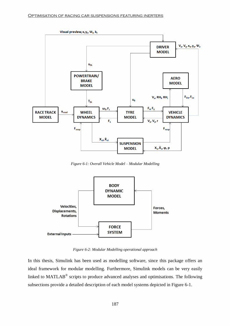
Optimisation of racing car suspensions featuring inerters
187
Figure 6-1: Overall Vehicle Model – Modular Modelling
Figure 6-2: Modular Modelling operational approach
In this thesis, Simulink has been used as modelling software, since this package offers an
ideal framework for modular modelling. Furthermore, Simulink models can be very easily
linked to MATLAB® scripts to produce advanced analyses and optimisations. The following
subsections provide a detailed description of each model systems depicted in Figure 6-1.

Chapter 6- Lap-Time Simulation
188
6.2.1. Vehicle and Wheel Dynamics Model
The basic requirement of the vehicle model is simplicity. As discussed in Chapter 5, model
complexity can increase substantially the computational time of simulation. The main goal of
this research work is to analyse the influence of suspension dynamics in the overall
performance of a race car. According to this premise, a lumped parameter single-track
vehicle model has been developed (see Figure 6-3). The model consists of three bodies: one
solid-rigid body that represents sprung mass ms and two more bodies that represent front and
rear wheels muf and mur respectively. The model depicted in Figure 6-3 has 9 DOFs. The
model allows translational motion of the vehicle in all three dimensions in space
(longitudinal, lateral and vertical motions) and rotations around two axes (yaw and pitch
motion). Front and rear unsprung wheels are connected to the main body via a suspension
system. Unsprung masses are assumed to have motion only in vertical direction. Moreover,
wheels are allowed to rotate only about the spin axis.
The model depicted in Figure 6-3 neglects rolling motions. As discussed in Chapter 5, the
results obtained from the ride analysis of the vehicle suspensions under rolling conditions
were not representative of the actual dynamic behaviour in roll of the physical car, so the
author decided that by neglecting this motion from the vehicle, improvements in
computational efficiency could be achieved without the loss of valuable information.
For such a model, the equations of motion (EOMs) can be expressed as a set of ODEs
describing the dynamics of the system. These equations of motion can be written in state-
space representation as follows:
With : n-dimensional state vector
: m-dimensional input vector
: independent variable time
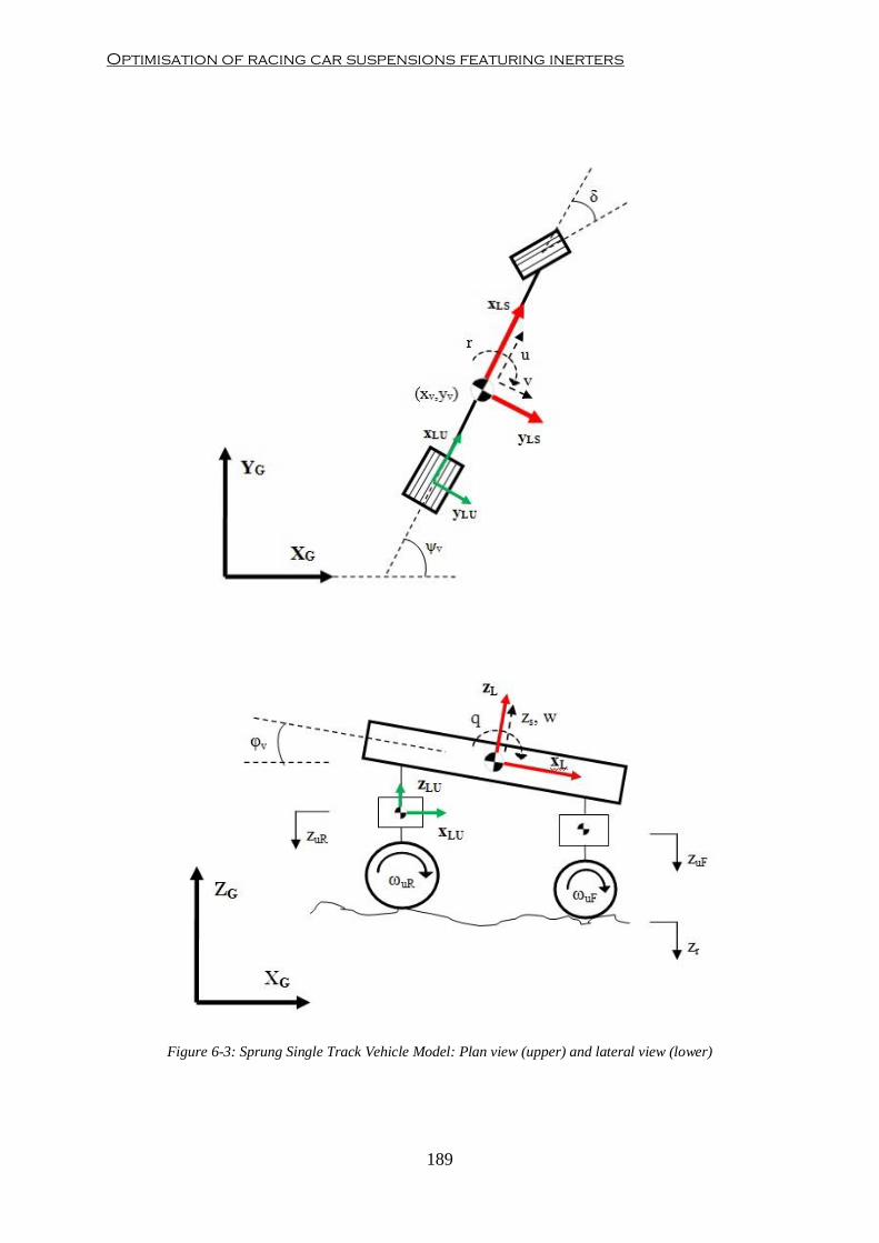
Optimisation of racing car suspensions featuring inerters
189
Figure 6-3: Sprung Single Track Vehicle Model: Plan view (upper) and lateral view (lower)

Chapter 6- Lap-Time Simulation
190
The state vector that defines the dynamic characteristic of the model depicted in Figure 6-3 is
composed of the following state variables:
Where vehicle heading angle
yaw rate
longitudinal velocity referenced to body local non-inertial frame
lateral velocity referenced to body local non-inertial frame
X-position in global inertial frame
Y-position in global inertial frame
pitch angle
pitch rate
chassis vertical position
chassis vertical velocity
front wheel spin velocity
rear wheel spin velocity
front unsprung mass vertical position
front unsprung mass vertical velocity
rear unsprung mass vertical position
rear unsprung mass vertical velocity
Two input controls have been considered in this vehicle model: longitudinal throttle/brake
control and steering control . Further discussions with regard to the input control
vector are covered in the Driver Model section.
Formal derivation of the equations of motion describing the dynamics of chassis and wheels
has been derived from the Lagrange Energy method for quasi-velocities (Genta & Morello,
2009). Detailed derivation of the equations of motion of the vehicle model can be found in
Appendix B.
6.2.2. Powertrain/Brake System Model
The powertrain model is composed of engine, gearbox and differential. Figure 6-4 illustrates
the layout of the powertrain. In most racing series, regulations rule that power can only be
delivered to one axle. In most track-based competitions, the rear axle is configured to produce
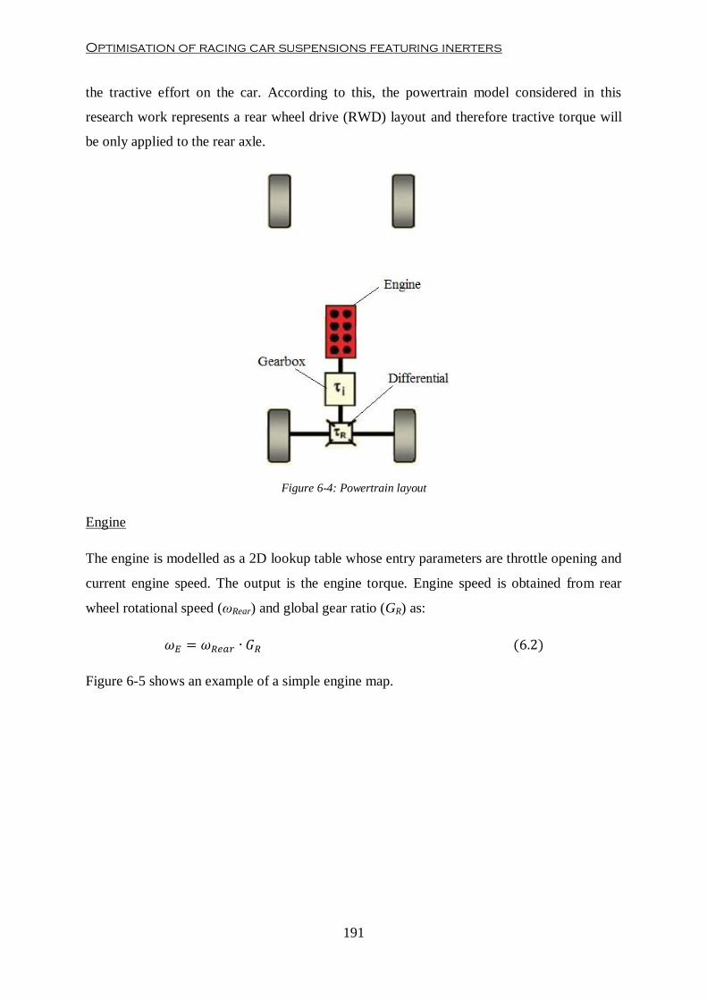
Optimisation of racing car suspensions featuring inerters
191
the tractive effort on the car. According to this, the powertrain model considered in this
research work represents a rear wheel drive (RWD) layout and therefore tractive torque will
be only applied to the rear axle.
Figure 6-4: Powertrain layout
Engine
The engine is modelled as a 2D lookup table whose entry parameters are throttle opening and
current engine speed. The output is the engine torque. Engine speed is obtained from rear
wheel rotational speed (ωRear) and global gear ratio (GR) as:
Figure 6-5 shows an example of a simple engine map.
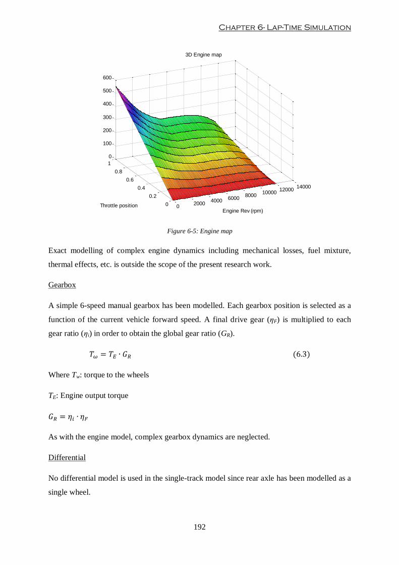
Chapter 6- Lap-Time Simulation
192
Figure 6-5: Engine map
Exact modelling of complex engine dynamics including mechanical losses, fuel mixture,
thermal effects, etc. is outside the scope of the present research work.
Gearbox
A simple 6-speed manual gearbox has been modelled. Each gearbox position is selected as a
function of the current vehicle forward speed. A final drive gear (ηF) is multiplied to each
gear ratio (ηi) in order to obtain the global gear ratio (GR).
Where Tw: torque to the wheels
TE: Engine output torque
As with the engine model, complex gearbox dynamics are neglected.
Differential
No differential model is used in the single-track model since rear axle has been modelled as a
single wheel.
02000
4000 60008000
1000012000
14000
0
0.2
0.4
0.6
0.8
1
0
100
200
300
400
500
600
Engine Rev (rpm)
3D Engine map
Throttle position
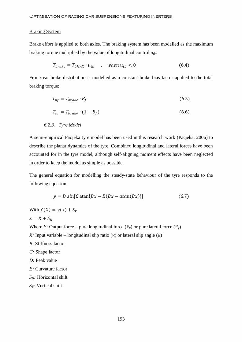
Optimisation of racing car suspensions featuring inerters
193
Braking System
Brake effort is applied to both axles. The braking system has been modelled as the maximum
braking torque multiplied by the value of longitudinal control utb:
Front/rear brake distribution is modelled as a constant brake bias factor applied to the total
braking torque:
6.2.3. Tyre Model
A semi-empirical Pacjeka tyre model has been used in this research work (Pacjeka, 2006) to
describe the planar dynamics of the tyre. Combined longitudinal and lateral forces have been
accounted for in the tyre model, although self-aligning moment effects have been neglected
in order to keep the model as simple as possible.
The general equation for modelling the steady-state behaviour of the tyre responds to the
following equation:
With
Where Y: Output force – pure longitudinal force (Fx) or pure lateral force (Fy)
X: Input variable – longitudinal slip ratio (κ) or lateral slip angle (α)
B: Stiffness factor
C: Shape factor
D: Peak value
E: Curvature factor
SH: Horizontal shift
SV: Vertical shift

Chapter 6- Lap-Time Simulation
194
Equation (6.7) creates a force under pure slip conditions. In order to account for combined
slip situations, the tyre model is extended to the following equation:
Where Fi: Longitudinal or lateral force in combined slip condition
Gij: Weighting factor
Fi0: Longitudinal or lateral force in pure slip condition
SVij: Vertical shift
Figure 6-6 shows an example of the characteristic lateral force created by a tyre as a function
of slip angle and slip ratio for a constant vertical load.
Figure 6-6: Tyre lateral force characteristic curve
The previous tyre model does not account for transient effects when variations in the input
variables occur. An extension of this model is to include the concept of relaxation length
(Pacjeka, 2006). In this research work, a semi nonlinear single contact point tyre model has
been usd to describe the transient behaviour of the tyre in both in-plane and out-of-plane
motions. Transient slip characteristics are approximated to a first-order differential equation
(see Equation (6.9)). The transient slip is then fed into the steady-state Magic Formula.
-50
0
50
-40
-20
0
20
40-4000
-2000
0
2000
4000
Slip angle (deg)
Tyre lateral force characteristic curve
Slip ratio (%)
Late
ral fo
rce (
N)
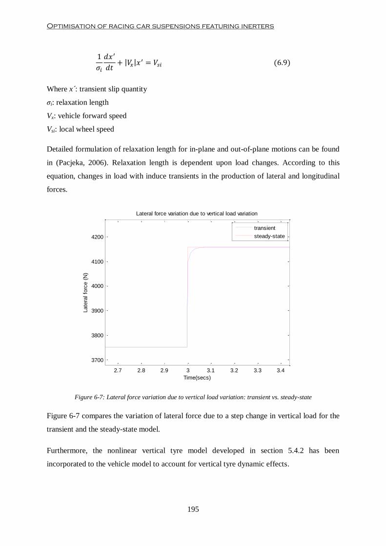
Optimisation of racing car suspensions featuring inerters
195
Where x´: transient slip quantity
σi: relaxation length
Vx: vehicle forward speed
Vsi: local wheel speed
Detailed formulation of relaxation length for in-plane and out-of-plane motions can be found
in (Pacjeka, 2006). Relaxation length is dependent upon load changes. According to this
equation, changes in load with induce transients in the production of lateral and longitudinal
forces.
Figure 6-7: Lateral force variation due to vertical load variation: transient vs. steady-state
Figure 6-7 compares the variation of lateral force due to a step change in vertical load for the
transient and the steady-state model.
Furthermore, the nonlinear vertical tyre model developed in section 5.4.2 has been
incorporated to the vehicle model to account for vertical tyre dynamic effects.
2.7 2.8 2.9 3 3.1 3.2 3.3 3.4
3700
3800
3900
4000
4100
4200
Lateral force variation due to vertical load variation
Time(secs)
Late
ral fo
rce (
N)
transient
steady-state
Chapter 6- Lap-Time Simulation
196
6.2.4. Aerodynamic model
Aerodynamics has a major impact in the performance of modern racing cars. The two major
aerodynamic actions considered in this model are the aerodynamic drag and downforce.
Lateral wind gust effects, as well as aerodynamic moments exerted on the body have been
neglected.
The total force exerted by the air flow into the chassis can be obtained as the integration of
the local pressure p over the whole vehicle surface area A:
Obtaining the exact pressure distribution around a surface such as race car bodywork is not
feasible due to the high amount of sensors that such task would require. In classical vehicle
dynamics literature, a semi-empirical approximate model has been used to describe
aerodynamic forces (Gillespie, 1992):
Where FDa: Aerodynamic drag force
FLa: Aerodynamic down-force
V: vehicle forward speed
A: vehicle frontal area
ρ: air density
CD, CL: drag and lift (or downforce) coefficients
Drag and lift coefficients must be experimentally obtained from the car through wind tunnel
or track testing or can be estimated through CFD simulation. These two empirical coefficients
depend on several factors such as body orientation and location with respect to ground levels,
aero-elasticity, throttle position, engine mapping, etc. In addition to this, the downforce
distribution between front and rear axles is a critical parameter in vehicle performance and
stability, especially at high speeds.

Optimisation of racing car suspensions featuring inerters
197
0
10
20
30
40
50 0
20
40
60
80
0.72
0.74
0.76
0.78
0.8
Rear Ride Height (mm)
Aero Drag Map
Front Ride Height (mm)
CdA
The simplest aerodynamic model is to assume that drag and lift coefficients and aerodynamic
distribution are constant regardless of any changes in the influencing factors. A more
complex model considers that changes in body location and attitude with respect to ground
level have an impact in the value of drag and lift coefficients and aero distribution. Thus,
these magnitudes are dependent upon body ride height at the CoG and body attitude.
Assuming that the chassis is a solid mass, body ride height at the CoG and body attitude can
be transformed into front and rear ride heights and therefore, construct the so-called ‘aero
maps’ with respect to these variables.
Figure 6-8 shows an example of aerodynamic drag and lift coefficients and aero distribution
maps with respect to front and rear ride heights.
Figure 6-8: Aerodynamic maps
0
10
20
30
40
50 0
20
40
60
80
1.5
2
2.5
3
3.5
Rear Ride Height (mm)
Aero Lift Map
Front Ride Height (mm)
ClA
0
10
20
30
40
50 0
20
40
60
80
25
30
35
40
45
50
Rear Ride Height (mm)
Aerodynamic Distribution Map
Front Ride Height (mm)
Aero
Dis
trib
ution (
%)
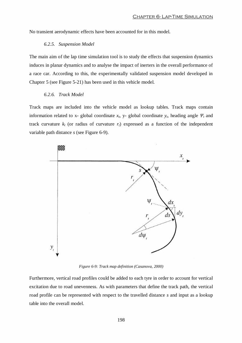
Chapter 6- Lap-Time Simulation
198
No transient aerodynamic effects have been accounted for in this model.
6.2.5. Suspension Model
The main aim of the lap time simulation tool is to study the effects that suspension dynamics
induces in planar dynamics and to analyse the impact of inerters in the overall performance of
a race car. According to this, the experimentally validated suspension model developed in
Chapter 5 (see Figure 5-21) has been used in this vehicle model.
6.2.6. Track Model
Track maps are included into the vehicle model as lookup tables. Track maps contain
information related to x- global coordinate xt, y- global coordinate yt, heading angle Ψt and
track curvature kt (or radius of curvature rt) expressed as a function of the independent
variable path distance s (see Figure 6-9).
Figure 6-9: Track map definition (Casanova, 2000)
Furthermore, vertical road profiles could be added to each tyre in order to account for vertical
excitation due to road unevenness. As with parameters that define the track path, the vertical
road profile can be represented with respect to the travelled distance s and input as a lookup
table into the overall model.

Optimisation of racing car suspensions featuring inerters
199
6.2.7. Driver Model
Race car drivers act as complex controllers always trying to stabilise the vehicle (plant)
whilst exploring the limits of grip to obtain the fastest lap time. It is out of the scope of the
present research work to investigate and produce a highly accurate driver model.
In this thesis, however, the driver is assumed to have control over throttle and brake controls
as well as steering inputs. Figure 6-10 shows a diagram of driver model operation.
Figure 6-10: Lap-time simulator driver model
Throttle/Brake control
Although real drivers are provided with different throttle and brake controls (different
pedals), the use of both controls simultaneously is rare in track-based racing series.
According to this, the present model assumes that the driver can actuate either the throttle or
the brake.
An additional yaw rate closed-loop proportional controller has been added to throttle/brake
input control. The driver then uses the actual yaw rate measurement to modulate the

Chapter 6- Lap-Time Simulation
200
throttle/brake input inputs (see Figure 6-10). The control law can be summarised in the
following equation:
With
r: Yaw rate
utbc: closed-loop throttle/brake control
Steering control
A nonlinear steering controller based on path preview has been used in this research work.
The main scheme of the controller proceeds from the path following steer model proposed in
(Casanova, 2000).
According to Casanova’s work, for a particular location along the trajectory of the vehicle, an
optical lever Lp can be defined as the product of a preview time Tp and vehicle forward speed
Vx. (see Figure 6-11).
Figure 6-11: Steering driver model (Casanova, 2000)
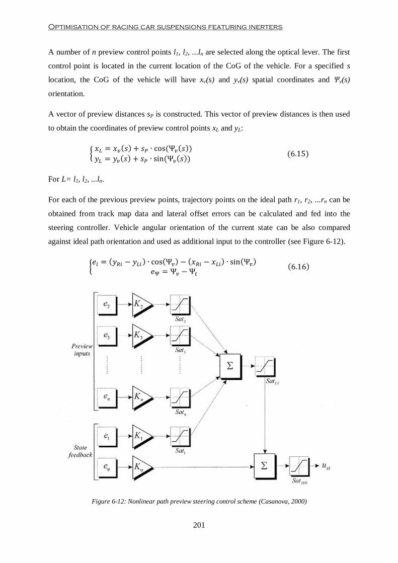
Optimisation of racing car suspensions featuring inerters
201
A number of n preview control points l1, l2, ...ln are selected along the optical lever. The first
control point is located in the current location of the CoG of the vehicle. For a specified s
location, the CoG of the vehicle will have xv(s) and yv(s) spatial coordinates and Ψv(s)
orientation.
A vector of preview distances sP is constructed. This vector of preview distances is then used
to obtain the coordinates of preview control points xL and yL:
For L= l1, l2, ...ln.
For each of the previous preview points, trajectory points on the ideal path r1, r2, ...rn can be
obtained from track map data and lateral offset errors can be calculated and fed into the
steering controller. Vehicle angular orientation of the current state can be also compared
against ideal path orientation and used as additional input to the controller (see Figure 6-12).
Figure 6-12: Nonlinear path preview steering control scheme (Casanova, 2000)

Chapter 6- Lap-Time Simulation
202
Finally, a set of control gains KΨ, K1, ..., Kn can be defined in order to construct steering
controller:
In addition to this, saturation limits are set to the individual controllers to prevent the tyres
from exceeding the limits of saturation and inducing under/oversteering moments.
6.3. Minimum Time Manoeuvre - Problem Statement
The problem of finding the minimum time manoeuvring (MTM) can be expressed as one of
Optimal Control (OC) theory (Casanova, 2000). In general OC theory, the OC problem can
be defined as determining a control u* that minimises a performance index J (Kirk, 2004)
subjected to a set of dynamic and boundary (equalities or/and inequalities) constraints.
Mathematically this can be expressed as:
In the case of transient lap-time simulation virtual tools, the OC problem can be stated as
finding a set of longitudinal and steering controls that minimises the time taken for a race car
to complete a lap around a race track. In this problem, the EOMs describing the behaviour of
the vehicle represent the set of dynamic constraints and the limits of the race track are
considered as boundary constraints.
In the following subsections, a detailed solution approach to the problem stated in equation
(6.18) will be presented.
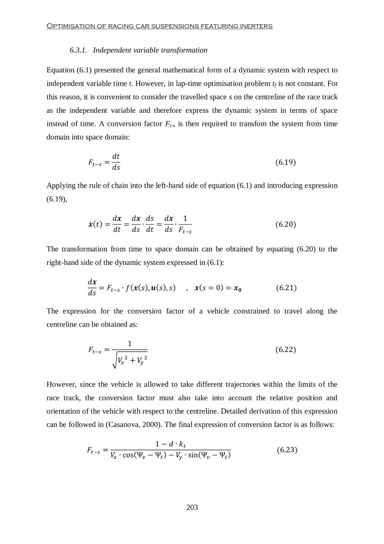
Optimisation of racing car suspensions featuring inerters
203
6.3.1. Independent variable transformation
Equation (6.1) presented the general mathematical form of a dynamic system with respect to
independent variable time t. However, in lap-time optimisation problem tf is not constant. For
this reason, it is convenient to consider the travelled space s on the centreline of the race track
as the independent variable and therefore express the dynamic system in terms of space
instead of time. A conversion factor Ft-s is then required to transfom the system from time
domain into space domain:
Applying the rule of chain into the left-hand side of equation (6.1) and introducing expression
(6.19),
The transformation from time to space domain can be obtained by equating (6.20) to the
right-hand side of the dynamic system expressed in (6.1):
The expression for the conversion factor of a vehicle constrained to travel along the
centreline can be obtained as:
However, since the vehicle is allowed to take different trajectories within the limits of the
race track, the conversion factor must also take into account the relative position and
orientation of the vehicle with respect to the centreline. Detailed derivation of this expression
can be followed in (Casanova, 2000). The final expression of conversion factor is as follows:

Chapter 6- Lap-Time Simulation
204
Where d: distance from vehicle CoG to track centreline expressed as:
6.3.2. Definition of the minimum lap-time cost function
As stated in previous sections, the overall aim of a lap-time simulation tool is to find a set of
control inputs so that the time taken for the race car to complete a lap around a circuit is
minimal. According to this goal, a mathematical cost function J that expresses time taken to a
car to complete a lap around a circuit must be obtained. From equation (6.19), time
differential dt can be calculated from independent space differential ds:
In computational methods, differential equations are equivalent to incremental expressions,
and therefore equation (6.25) can be re-written as:
A time vector can be obtained for the cumulative sum of time increments ∆t as:
Finally, the cost function J can be expressed as the last value of time vector obtained from
equation (6.27):
6.4. Multilevel optimisation algorithm - Solution Method
A method must be developed in order to solve the MTM problem characterised in section 6.3.
Several approaches have been reviewed in Chapter 2. In previous work, driver longitudinal
and steering input controls have been assumed to be independent between each other and the
problem of obtaining the optimal racing line came implicitly solved when attempting to
minimise lap time (Casanova, 2000; Kelly, 2008). According to these approaches, the general
OC problem formulated in section 6.3 is transformed into a constrained non-linear
programming (NLP) problem in which the search space is composed by a set of discretised
Optimisation of racing car suspensions featuring inerters
205
longitudinal and steering input controls subjected to the dynamics of the vehicle model and
constrained by the limits of the race track.
A number of issues must be addressed when developing a solution approach to the OTM
problem, the first of these being that the solution method must be robust. On the limit of
adhesion, the use of completely decoupled control inputs causes vehicle instabilities (vehicle
going off the line or vehicle spinning off). Real drivers use a combination of throttle/brake
and steering controls in order to simultaneously maintain vehicle stability and negotiate the
race track as fast as possible. In order to overcome robustness issues, Casanova (2000)
proposed a multiple shooting algorithm in which the race track is split into sections short
enough in order to prevent the vehicle from becoming unstable. This method introduces
additional continuity constraints to the problem. Kelly (2008) defined stability constraints and
used a Model Predictive Control (MPC) algorithm to provide the driver model with a preview
horizon. Secondly, computational efficiency issues must also be addressed. When
transcribing the OC problem to a Nonlinear Programming (NLP) problem, NLP solvers
augment the performance index or cost function with search space variables and constraints,
therefore increasing the complexity and number of DOFs of the augmented cost function.
Both previous solution approaches required the use of independent longitudinal and steering
control inputs as search space variables. Furthermore, in order to increase the robustness of
the algorithm, both methods required the introduction of additional constraints in order to
limit the development of dynamic instabilities.
Following the research work carried out in the field, a direct method has been used to
transcribe the OC problem into a NLP problem. Once the problem has been transcribed into a
NLP problem, a nonlinear constrained optimisation solver is then used to obtain the solution
of the NLP problem. In this thesis, a Sequential Quadratic Programming (SQP) algorithm
built in MATLAB® function fmincon has been used as NLP solver (The MathWorks Inc.,
2010).
In the present work, a novel multilevel optimisation algorithm (MLOA) has been proposed
with the aim to increase the robustness and efficiency of the solution method. MLOA
proposes an alternative transcription method from OC problem to NLP program. MLOA uses
a closed-loop driver steering control model to tackle the racing line optimisation problem and
a coupled longitudinal control model to minimise the lap-time.
MLOA can be split into two solution levels:

Chapter 6- Lap-Time Simulation
206
Trajectory Planning
Lap Time Minimisation
The following sections detail the transcription procedure from the initial OC problem to the
NLP problem.
6.4.1. MLOA level 1: Trajectory Planning
The time taken to complete a lap depends on the distance travelled and the speed carried by
the race car. According to this principle, the driver will be able to reduce lap time whenever it
reduces the travelled distance within the confines of the race track and/or it increases its
forward speed. Under this premise, the optimal racing line is considered to lie within the
shortest possible path (SP) and a line that produces the highest possible speed, i.e. the
minimum curvature path (MCP). Hence, although the actual optimal racing line depends on
the complex dynamic behaviour of the race car, the problem of trajectory planning will be
bounded optimisation problem between SP and MCP lines.
Finding the SP and MCP racing lines can be considered as a pure geometric constrained
optimisation problem since the solutions must always lie inside the limits of the circuit. In
both cases, the optimisation problem is transcribed into a NLP problem. In order to carry out
this transcription, the track is discretised into a finite number of segments. Each of the
discrete trajectory point can be characterised by the spatial coordinates of the lower and upper
bounds of track, as shown in Figure 6-13:
Figure 6-13: Race track discretisation (Braghin, et al., 2008)
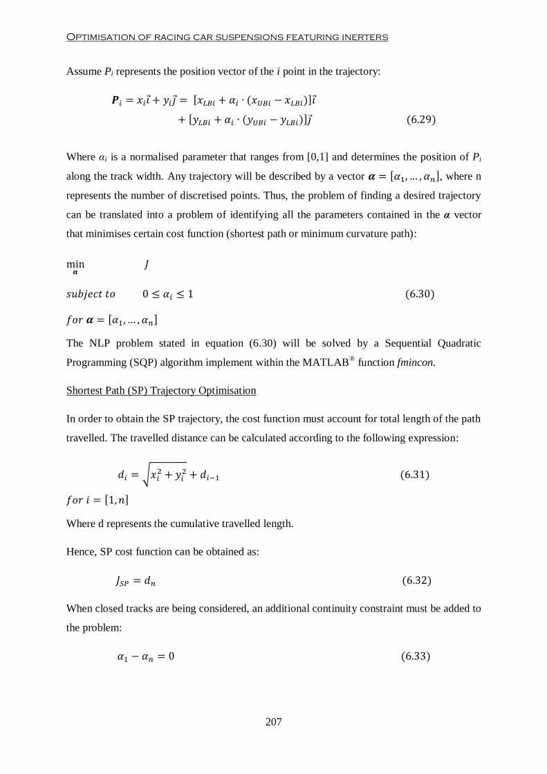
Optimisation of racing car suspensions featuring inerters
207
Assume Pi represents the position vector of the i point in the trajectory:
Where αi is a normalised parameter that ranges from [0,1] and determines the position of Pi
along the track width. Any trajectory will be described by a vector , where n
represents the number of discretised points. Thus, the problem of finding a desired trajectory
can be translated into a problem of identifying all the parameters contained in the α vector
that minimises certain cost function (shortest path or minimum curvature path):
The NLP problem stated in equation (6.30) will be solved by a Sequential Quadratic
Programming (SQP) algorithm implement within the MATLAB® function fmincon.
Shortest Path (SP) Trajectory Optimisation
In order to obtain the SP trajectory, the cost function must account for total length of the path
travelled. The travelled distance can be calculated according to the following expression:
Where d represents the cumulative travelled length.
Hence, SP cost function can be obtained as:
When closed tracks are being considered, an additional continuity constraint must be added to
the problem:
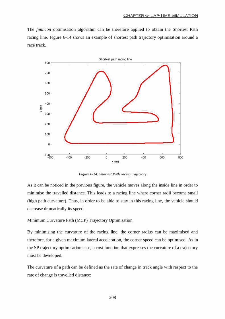
Chapter 6- Lap-Time Simulation
208
The fmincon optimisation algorithm can be therefore applied to obtain the Shortest Path
racing line. Figure 6-14 shows an example of shortest path trajectory optimisation around a
race track.
Figure 6-14: Shortest Path racing trajectory
As it can be noticed in the previous figure, the vehicle moves along the inside line in order to
minimise the travelled distance. This leads to a racing line where corner radii become small
(high path curvature). Thus, in order to be able to stay in this racing line, the vehicle should
decrease dramatically its speed.
Minimum Curvature Path (MCP) Trajectory Optimisation
By minimising the curvature of the racing line, the corner radius can be maximised and
therefore, for a given maximum lateral acceleration, the corner speed can be optimised. As in
the SP trajectory optimisation case, a cost function that expresses the curvature of a trajectory
must be developed.
The curvature of a path can be defined as the rate of change in track angle with respect to the
rate of change is travelled distance:
-600 -400 -200 0 200 400 600 800-100
0
100
200
300
400
500
600
700
800Shortest path racing line
x (m)
y (
m)
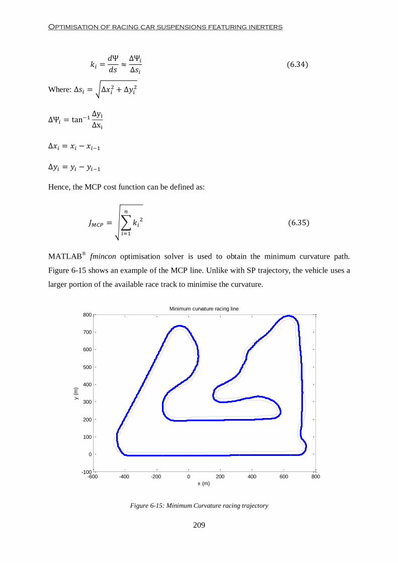
Optimisation of racing car suspensions featuring inerters
209
Where:
Hence, the MCP cost function can be defined as:
MATLAB®
fmincon optimisation solver is used to obtain the minimum curvature path.
Figure 6-15 shows an example of the MCP line. Unlike with SP trajectory, the vehicle uses a
larger portion of the available race track to minimise the curvature.
Figure 6-15: Minimum Curvature racing trajectory
-600 -400 -200 0 200 400 600 800-100
0
100
200
300
400
500
600
700
800Minimum curvature racing line
x (m)
y (
m)

Chapter 6- Lap-Time Simulation
210
6.4.2. MLOA level 2: Lap Time Minimisation
The minimum time manoeuvring problem can be considered as a dynamic problem since the
optimal solution is strongly influenced by the dynamic behaviour of the race car. In this
second optimisation stage, the optimal racing line can be assumed to be a linear combination
between the SP and the MCP trajectories (Braghin, et al., 2008). Mathematically, this can be
expressed as follows:
Where OT: Optimal Trajectory
ε: normalised weighting factor
In a general MTM problem where the longitudinal and steering input controls have been
discretised at p and n points respectively, the search space presents p+n degrees of freedom,
due to the fact that open-loop driver control inputs has been used. However, if a closed-loop
steering control is used, a vehicle should be able to follow a prescribed trajectory with no
need to explicitly specify a set of open-loop steering controls.
According to this, the multilevel optimisation algorithm (MLOA) developed in this research
work proposes that, with the aid of the steering driver control presented in section 6.2, the n
steering control input points can be substituted by the weighting factor ε. Hence, the problem
size can be drastically reduced and therefore, the efficiency of the algorithm can be increased.
Furthermore, since the vehicle is now constrained to follow a trajectory that is bounded
between the shortest path and the minimum curvature trajectories, no boundary constrain are
required to define the OC problem. Thus, MLOA transforms the constrained OC problem
with p+n DOFs into an unconstrained OC problem with p+1 DOFs.
Moreover, since the throttle/brake input control is coupled with a yaw rate controller, the
driver can self-modulate the amount of throttle/brake applied under high lateral acceleration
conditions, therefore increasing the stability of the vehicle and making the algorithm more
robust.
6.4.3. Discretisation Scheme
The transcription of the OC problem into a NLP problem requires the parametrisation of the
control variables. The discretisation process involves defining a set of finite number of

Optimisation of racing car suspensions featuring inerters
211
control points, which will then be used by the NLP solver as input variables to obtain an
optimised solution. According to the MLOA presented in previous sections, only longitudinal
control inputs utb and racing line weighting factor ε are required to define the OC problem,
since lateral controls are determined by the closed-loop driver controller.
Throttle/Brake control input utb
First, the longitudinal control history is discretised into p control points, so that:
The number of discretised control inputs p defines the size of the optimisation problem.
Hence, in order to reduce the problem size, a variable discretisation scheme can be selected.
According to this, the density of the grid could be increased in areas of the track where the
rate of control change is expected to be higher, e. g. braking points or throttle/brake
modulation areas. In areas where controls are expected to remain constant, density could be
therefore reduced. An example of a variable control input discretisation scheme is shown in
Figure 6-16.
Figure 6-16: Variable control input discretisation scheme
-600 -400 -200 0 200 400 600 800-100
0
100
200
300
400
500
600
700
800Control input discretisation scheme
x(m)
y(m
)
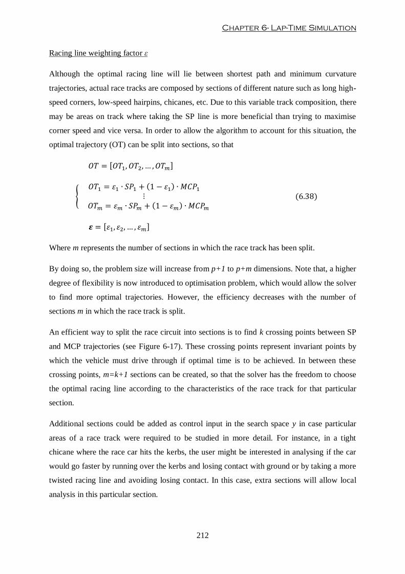
Chapter 6- Lap-Time Simulation
212
Racing line weighting factor ε
Although the optimal racing line will lie between shortest path and minimum curvature
trajectories, actual race tracks are composed by sections of different nature such as long high-
speed corners, low-speed hairpins, chicanes, etc. Due to this variable track composition, there
may be areas on track where taking the SP line is more beneficial than trying to maximise
corner speed and vice versa. In order to allow the algorithm to account for this situation, the
optimal trajectory (OT) can be split into sections, so that
Where m represents the number of sections in which the race track has been split.
By doing so, the problem size will increase from p+1 to p+m dimensions. Note that, a higher
degree of flexibility is now introduced to optimisation problem, which would allow the solver
to find more optimal trajectories. However, the efficiency decreases with the number of
sections m in which the race track is split.
An efficient way to split the race circuit into sections is to find k crossing points between SP
and MCP trajectories (see Figure 6-17). These crossing points represent invariant points by
which the vehicle must drive through if optimal time is to be achieved. In between these
crossing points, m=k+1 sections can be created, so that the solver has the freedom to choose
the optimal racing line according to the characteristics of the race track for that particular
section.
Additional sections could be added as control input in the search space y in case particular
areas of a race track were required to be studied in more detail. For instance, in a tight
chicane where the race car hits the kerbs, the user might be interested in analysing if the car
would go faster by running over the kerbs and losing contact with ground or by taking a more
twisted racing line and avoiding losing contact. In this case, extra sections will allow local
analysis in this particular section.
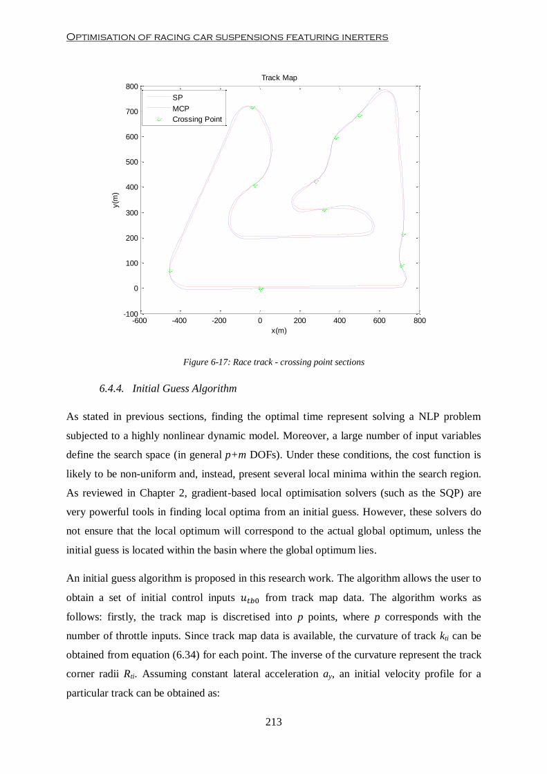
Optimisation of racing car suspensions featuring inerters
213
Figure 6-17: Race track - crossing point sections
6.4.4. Initial Guess Algorithm
As stated in previous sections, finding the optimal time represent solving a NLP problem
subjected to a highly nonlinear dynamic model. Moreover, a large number of input variables
define the search space (in general p+m DOFs). Under these conditions, the cost function is
likely to be non-uniform and, instead, present several local minima within the search region.
As reviewed in Chapter 2, gradient-based local optimisation solvers (such as the SQP) are
very powerful tools in finding local optima from an initial guess. However, these solvers do
not ensure that the local optimum will correspond to the actual global optimum, unless the
initial guess is located within the basin where the global optimum lies.
An initial guess algorithm is proposed in this research work. The algorithm allows the user to
obtain a set of initial control inputs from track map data. The algorithm works as
follows: firstly, the track map is discretised into p points, where p corresponds with the
number of throttle inputs. Since track map data is available, the curvature of track kti can be
obtained from equation (6.34) for each point. The inverse of the curvature represent the track
corner radii Rti. Assuming constant lateral acceleration ay, an initial velocity profile for a
particular track can be obtained as:
-600 -400 -200 0 200 400 600 800-100
0
100
200
300
400
500
600
700
800
x(m)
y(m
)
Track Map
SP
MCP
Crossing Point

Chapter 6- Lap-Time Simulation
214
Note that, in straight lines, and therefore, as well. In order to prevent
this situation a limit forward velocity can be defined so that VxRefi ≤ Vx0max. Figure 6-18 shows
an example of the estimated vehicle speed profile for the Bahrain International GP circuit.
Figure 6-18: Initial vehicle speed profile estimation
A simple closed-loop PID controller has been enabled into the vehicle model so that the
estimated vehicle speed profile can be used to obtain the set of initial control inputs utb0
according to the diagram depicted in Figure 6-19. Results of the simulation are shown in
Figure 6-20 to Figure 6-22.
-400 -200 0 200 400 600 800
0
200
400
600
800
x(m)
y(m
)
Track map
0 1000 2000 3000 4000 5000 600030
40
50
60
70
80
90
s(m)
Vx (
m/s
)
Estimated vehicle speed profile
Start 1
2
3
4 5
6
7
2
1 3 4
5 6 7

Optimisation of racing car suspensions featuring inerters
215
Figure 6-19: Initial control input guess diagram
Figure 6-20 shows a set of initial throttle/brake control inputs utb0. As it can be observed from
this graph, the driver spends most of the time on throttle in an attempt to maximise forward
speed. Brake is applied in small portions of time in order to accommodate the speed of the
vehicle to handle the corners.
Figure 6-21 shows a comparison between the estimated velocity profile and the real one
obtained through simulation. As it can be noticed, although the vehicle is able to match the
estimated speed profile at low speeds, due to dynamic limitations of the race car, real forward
velocity will never reach maximum estimated speed. A similar situation can be noticed in
Figure 6-22. At some points in the circuit, the car is running off the line, particularly in turns
1, 7 and 8. This is due to fact that the estimated forward speed profile has been calculated
assuming that, when the car is cornering, all force available from the tyre is used to generate
lateral acceleration. However, in the case of the dynamic simulation, the tyre is producing
lateral as well as longitudinal forces. This reduces the capability of the tyres to produce
enough lateral acceleration so that the vehicle can track the racing line.
This set of control inputs produces a trajectory that violates the limits of the race track. Since
the set of control inputs obtained following this algorithm is then used as initial guess of the
NLP problem, little attention must be paid to the produced trajectory. However, in order to
ensure that the NLP solver does not produce an optimised trajectory that potentially could
violate the limits of the race track; the performance cost function of equation (6.28) will
incorporate a term that accounts for the deviation of the vehicle from the optimal racing line.
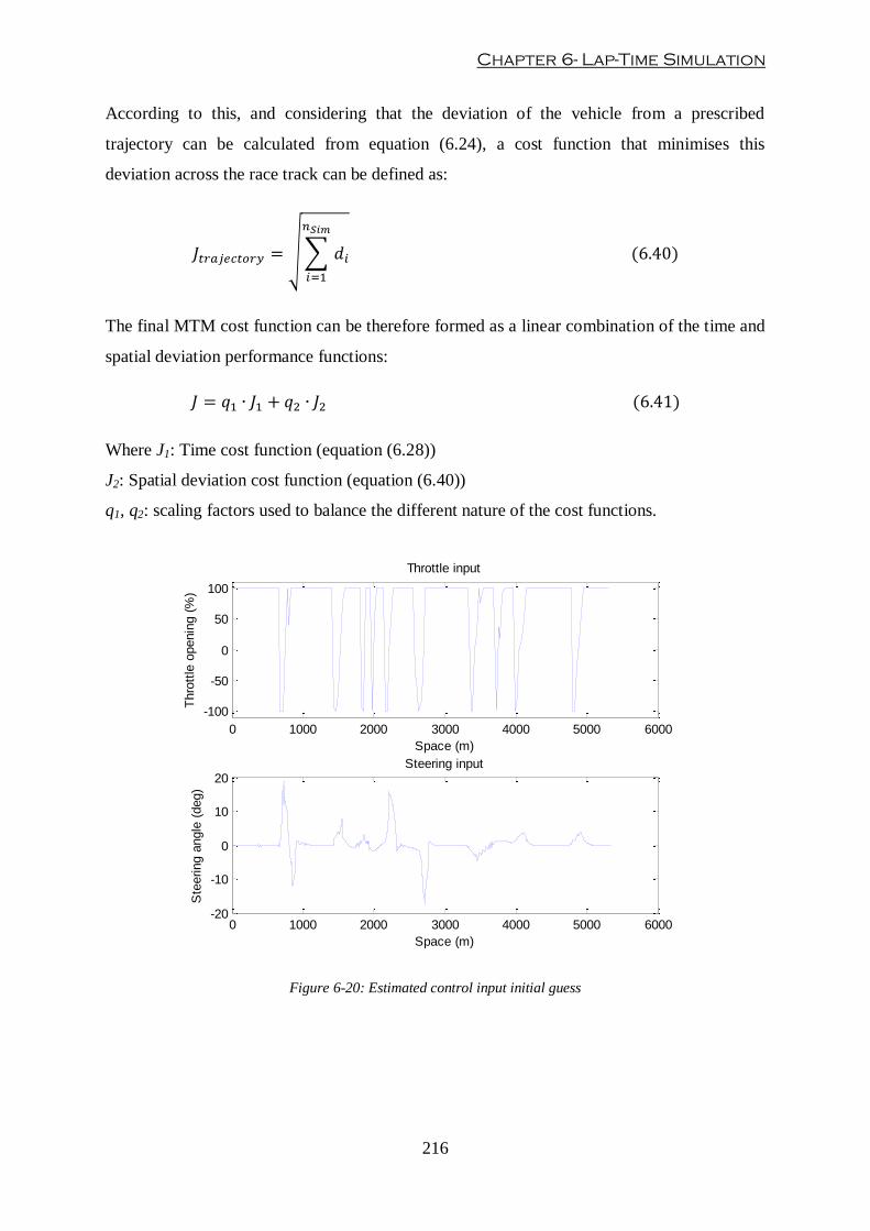
Chapter 6- Lap-Time Simulation
216
According to this, and considering that the deviation of the vehicle from a prescribed
trajectory can be calculated from equation (6.24), a cost function that minimises this
deviation across the race track can be defined as:
The final MTM cost function can be therefore formed as a linear combination of the time and
spatial deviation performance functions:
Where J1: Time cost function (equation (6.28))
J2: Spatial deviation cost function (equation (6.40))
q1, q2: scaling factors used to balance the different nature of the cost functions.
Figure 6-20: Estimated control input initial guess
0 1000 2000 3000 4000 5000 6000
-100
-50
0
50
100
Throttle input
Space (m)
Thro
ttle
openin
g (
%)
0 1000 2000 3000 4000 5000 6000-20
-10
0
10
20Steering input
Space (m)
Ste
ering a
ngle
(deg)
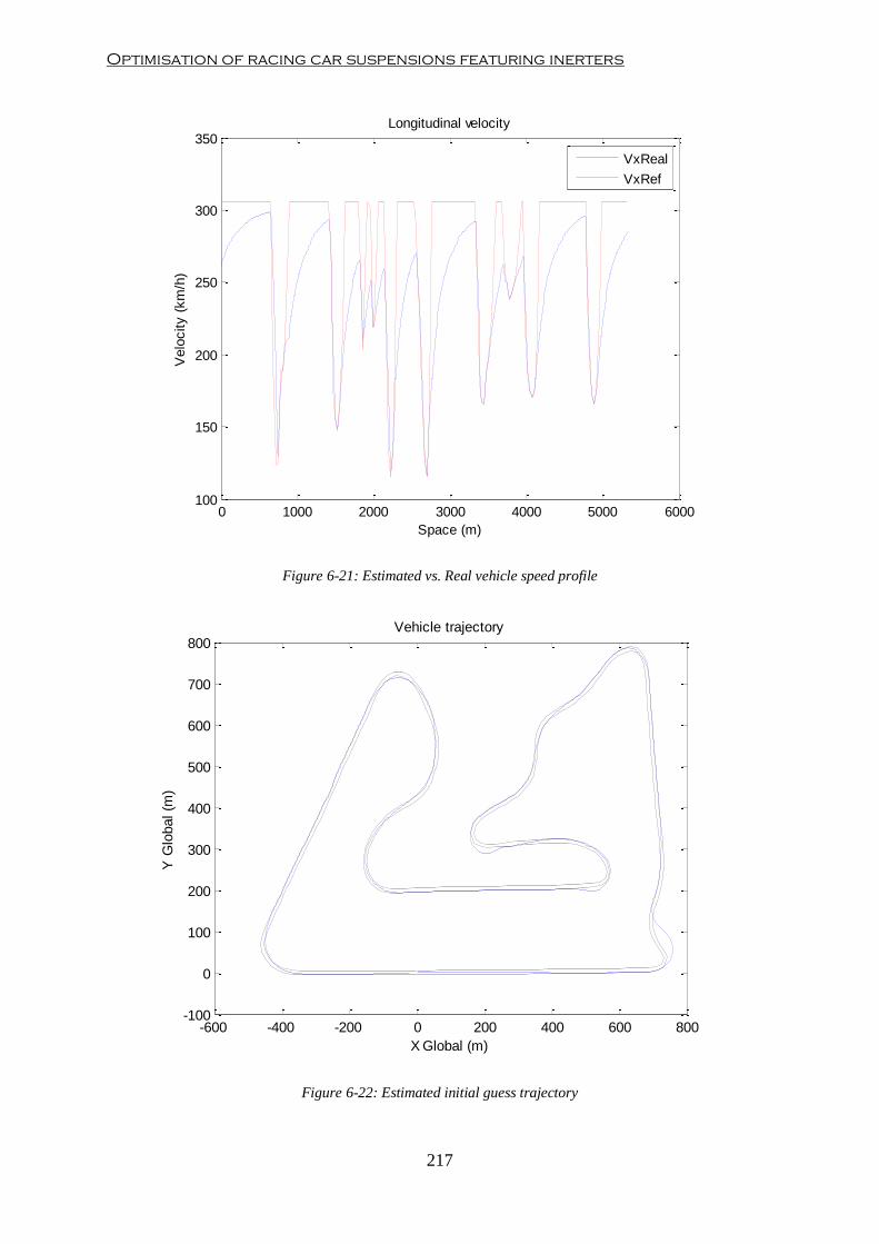
Optimisation of racing car suspensions featuring inerters
217
Figure 6-21: Estimated vs. Real vehicle speed profile
Figure 6-22: Estimated initial guess trajectory
0 1000 2000 3000 4000 5000 6000100
150
200
250
300
350Longitudinal velocity
Space (m)
Velo
city (
km
/h)
VxReal
VxRef
-600 -400 -200 0 200 400 600 800-100
0
100
200
300
400
500
600
700
800Vehicle trajectory
X Global (m)
Y G
lobal (m
)

Chapter 6- Lap-Time Simulation
218
Hence, the MTM problem can be summarised in NLP problem as follows:
As explained at the beginning of the section, the NLP problem can be solved with a SQP
algorithm built in fmincon MATLAB® function. The following section presents practical case
study of the lap time simulation tool developed.
6.5. Case Study
In this section, the lap time simulation virtual tool developed in previous sections is used in a
practical case study. The vehicle model developed in section 6.2 has been driven along a
Bahrain GP Circuit as fast as possible. First, the parameters required to set up the
optimisation problem are discussed. Secondly, optimal solutions from the optimisation solver
are analysed.
6.5.1. Optimal Time Manoeuvring problem set-up
NLP solvers, such as the SQP used in this thesis, require a number of optimisation parameters
to be defined. The selection of these parameters will have an important impact in the
performance of the algorithm. The optimisation parameters required to the set-up the
optimisation are:
Number of throttle/brake input control discretisation points.
Number of race track sections.
Dynamic model integration solver and step size.
Stopping criteria.
As explained in section 6.4.3, the number of controls inputs defines the size of the
optimisation. On one end, a fine control input grid will increase the accuracy of the optimal
solution but the efficiency of the solver will decrease, since the number of function
evaluations per optimisation iteration increases linearly with the problem size. On the other
end, a burden input control grid will increase efficiency of the solver but it could lead to

Optimisation of racing car suspensions featuring inerters
219
vehicle stability issues, since input control changes would not react fast enough to the
requirements of the model. Variable-spaced input controls are used as a compromised
solution between both previous cases. In this example, controls are placed at a relative
distance in the range from 8 to 80 m as shown in Figure 6-16. According to this discretisation
grid, the total number of control inputs for the Bahrain GP Circuit is 193.
The total dimension of the optimisation problem also is affected by the number of sections in
which the race track is divided. According to the crossing point section algorithm introduced
in section 6.4.3, the race track has been split into 7 sections leading to 7 racing line weighting
factors. Figure 6-23 shows the sections into which the race track has been divided for this
particular example. By adding the weighting factors to the control input grid, the total number
of independent optimisation variables is therefore 200.
Figure 6-23: Bahrain GP track sections
The selection of the adequate integration method and integration step size will affect the
accuracy of the simulation of the dynamic vehicle model (numerical stability) and the
computational efficiency of the solver. Simulink allows the configuration of different
numerical integration solvers. In this example, a fixed-step 4th
-order Runge-Kutta integration
solver has been used because it offers a good compromise between numerical stability and
-600 -400 -200 0 200 400 600 8000
100
200
300
400
500
600
700
800Track map sections
x(m)
y(m
)
S1
S2
S3
S4
S5
S6
S7
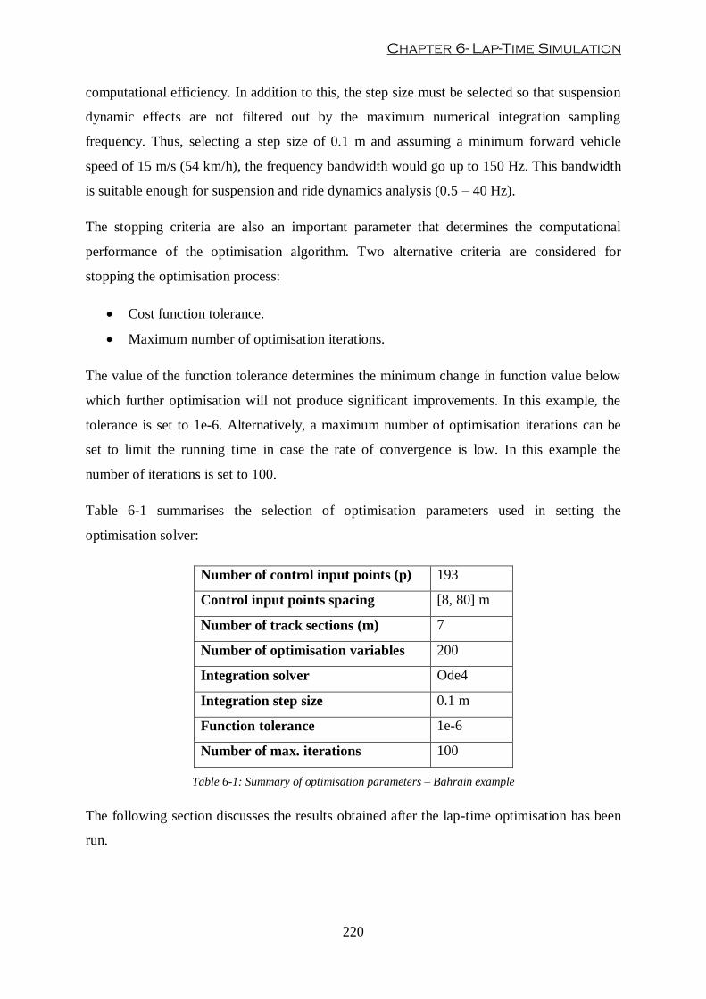
Chapter 6- Lap-Time Simulation
220
computational efficiency. In addition to this, the step size must be selected so that suspension
dynamic effects are not filtered out by the maximum numerical integration sampling
frequency. Thus, selecting a step size of 0.1 m and assuming a minimum forward vehicle
speed of 15 m/s (54 km/h), the frequency bandwidth would go up to 150 Hz. This bandwidth
is suitable enough for suspension and ride dynamics analysis (0.5 – 40 Hz).
The stopping criteria are also an important parameter that determines the computational
performance of the optimisation algorithm. Two alternative criteria are considered for
stopping the optimisation process:
Cost function tolerance.
Maximum number of optimisation iterations.
The value of the function tolerance determines the minimum change in function value below
which further optimisation will not produce significant improvements. In this example, the
tolerance is set to 1e-6. Alternatively, a maximum number of optimisation iterations can be
set to limit the running time in case the rate of convergence is low. In this example the
number of iterations is set to 100.
Table 6-1 summarises the selection of optimisation parameters used in setting the
optimisation solver:
Number of control input points (p) 193
Control input points spacing [8, 80] m
Number of track sections (m) 7
Number of optimisation variables 200
Integration solver Ode4
Integration step size 0.1 m
Function tolerance 1e-6
Number of max. iterations 100
Table 6-1: Summary of optimisation parameters – Bahrain example
The following section discusses the results obtained after the lap-time optimisation has been
run.

Optimisation of racing car suspensions featuring inerters
221
6.5.2. Bahrain GP Circuit – Results
The lap-time optimisation tool has been run for a high-downforce generic racing car on the
Bahrain GP Circuit. The race track presents the following characteristics:
Race Track Length 5412 m
Total number of corners 15
Right-hand corners 9
Left-hand corners 6
Total number of straights 4
Longest straight length 1090 m
Average Width 18 m
Table 6-2: Bahrain GP track main characteristics
For the race track characterised in Table 6-2, a Dell T1500 Precision computer with an Intel
i5 processor has been used. The computation was about 4 hours and the optimal solution was
produced after 38 optimisation iterations. The optimal lap time is shown in Table 6-3.
Lap Time Optimisation Summary – Bahrain GP Circuit
Lap Time 1’25’’340
Table 6-3: Summary of lap-time optimisation
Figure 6-24 shows the time histories for throttle/brake and steering inputs achieved by the
virtual driver model when driving the race car on the limit of performance. Note that, the
longitudinal control input time history is noisy, especially when the longitudinal input is in a
region close to full throttle. This is due to several reasons: firstly, when the car is exiting a
corner, tyres are still producing a certain amount of lateral force, therefore the driver must
modulate the throttle input in order to prevent the vehicle from spinning off. Secondly, due to
road unevenness, vertical load on the tyres fluctuates constantly (see Figure 6-32), tyre slip
ratios are also fluctuating (see Figure 6-28) and therefore there is a variation on the available
longitudinal force generated by tyres. Finally, as explained in section 6.2.7, e throttle/brake
input is linked to the steering control via a yaw rate proportional control. Thus, variations in
yaw rate conditions induce the driver to modulate the throttle/brake input.
Figure 6-25 shows that the optimisation solver manages to produce an optimal trajectory
within the limits of the race. Due to the nature of the generic race car configuration used in

Chapter 6- Lap-Time Simulation
222
this example, the optimal trajectory followed by the vehicle is close to the MCP trajectory,
especially in sections with high-speed corners such as turns 11, 12, 14 and 15.
Figure 6-26 and Figure 6-29 represent forward speed, vehicle attitude and vertical position
respectively. These graphs show the strong influence of aerodynamics in chassis attitude and
vertical position. Figure 6-30 shows how aerodynamic lift coefficient and aero distribution
varies with ride height and pitch angle. From these graphs, an inversely proportional
relationship between ride height and speed can be observed. In turn, this variation in ride
height affects the production of aerodynamic downforce. For instance, a reduction of about
15% of lift coefficient is experienced on low-speed turns (distance travelled 800, 2250 and
2700 m) can be noticed in Figure 6-30. Figure 6-32 represents the history of normal load
applied at the tyre contact patch. As it can be observed, normal loads increase drastically with
speed, which leads to higher longitudinal and lateral accelerations. A g-g-V diagram has been
produced in Figure 6-31. As it can be observed, the maximum available longitudinal and
lateral tyre forces increase as speed increases. Hence, this highlights that aerodynamics play
important role in the overall performance of the race vehicle.
Finally, Figure 6-29 and Figure 6-32 are characterised by a high frequency content
superimposed to the much lower frequency history dictated by the speed trace. This effect is
due to the interaction between road inputs and suspension dynamics. Road unevenness
induces high frequency vibrations on the chassis which, in turn, excites tyres and modifies the
dynamic load at the contact patches. Figure 6-33 depicts the frequency response of front and
rear dynamic contact patch loads. In this graph, two resonant modes can be identified for both
axles: firstly, a body mode occurring at around 3 Hz, and, secondly, a hub mode at about 15
Hz. Hence, the main goal of a race car suspension is to filter out as much high frequency
noise content as possible, so that vibrations induced by uneven road profiles do not cause a
significant impact in the dynamics of the vehicle.
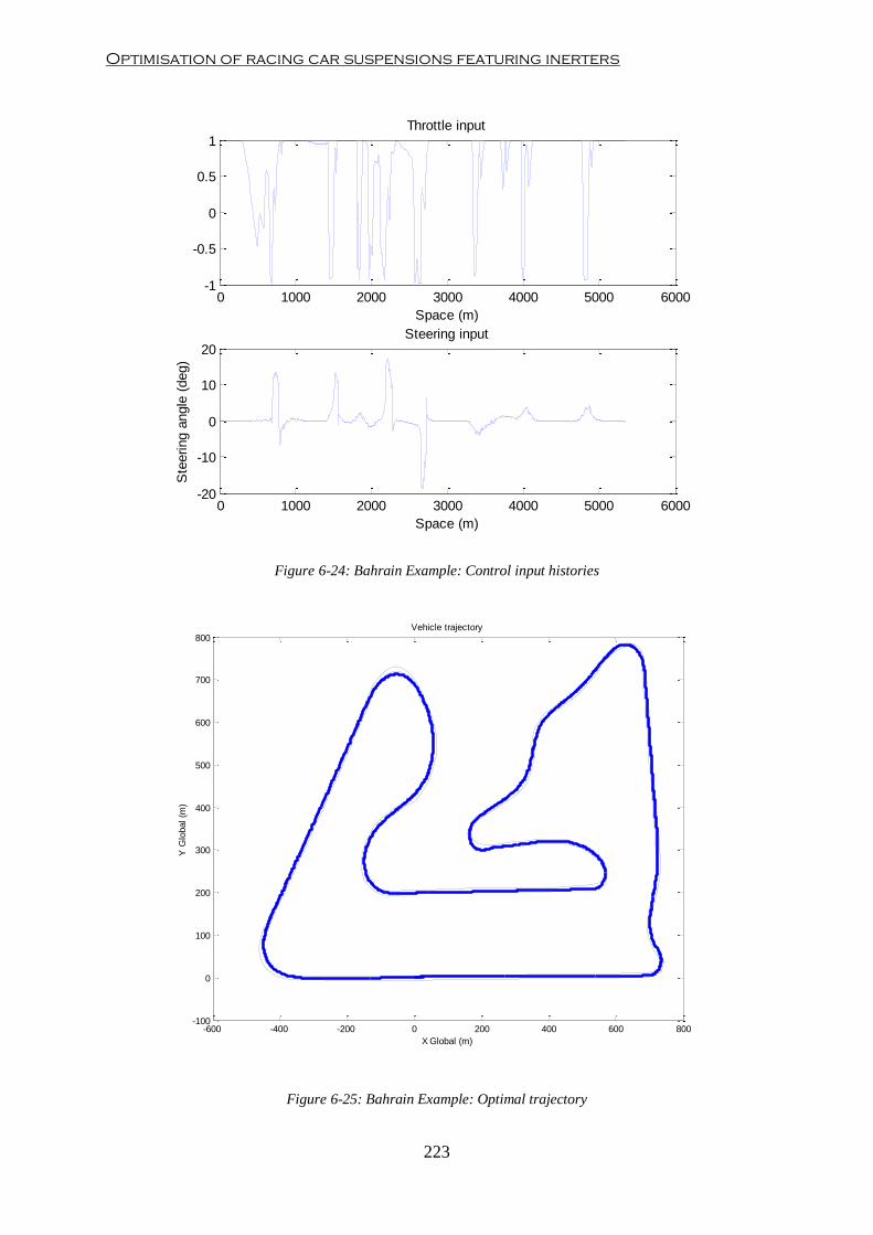
Optimisation of racing car suspensions featuring inerters
223
Figure 6-24: Bahrain Example: Control input histories
Figure 6-25: Bahrain Example: Optimal trajectory
0 1000 2000 3000 4000 5000 6000-1
-0.5
0
0.5
1Throttle input
Space (m)
0 1000 2000 3000 4000 5000 6000-20
-10
0
10
20Steering input
Space (m)
Ste
ering a
ngle
(deg)
-600 -400 -200 0 200 400 600 800-100
0
100
200
300
400
500
600
700
800Vehicle trajectory
X Global (m)
Y G
lobal (m
)

Chapter 6- Lap-Time Simulation
224
Figure 6-26: Bahrain Example: Forward speed profile and gear change history
Figure 6-27: Bahrain Example: Front and rear slip angle histories
0 1000 2000 3000 4000 5000 60000
100
200
300Longitudinal velocity
Space (m)
Velo
city (
km
/h)
0 1000 2000 3000 4000 5000 60002
3
4
5
6Gear changes
Space (m)
Gear
Positio
n
0 1000 2000 3000 4000 5000 6000-20
-10
0
10
20Front Slip Angle
Space (m)
Slip
Angle
(deg)
0 1000 2000 3000 4000 5000 6000-10
-5
0
5
10Rear Slip Angle
Space (m)
Slip
Angle
(deg)
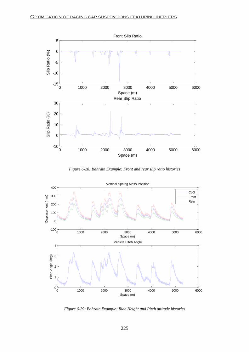
Optimisation of racing car suspensions featuring inerters
225
Figure 6-28: Bahrain Example: Front and rear slip ratio histories
Figure 6-29: Bahrain Example: Ride Height and Pitch attitude histories
0 1000 2000 3000 4000 5000 6000-15
-10
-5
0
5Front Slip Ratio
Space (m)
Slip
Ratio (
%)
0 1000 2000 3000 4000 5000 6000-10
0
10
20
30Rear Slip Ratio
Space (m)
Slip
Ratio (
%)
0 1000 2000 3000 4000 5000 60000
1
2
3
4Vehicle Pitch Angle
Space (m)
Pitch A
ngle
(deg)
0 1000 2000 3000 4000 5000 6000-100
0
100
200
300
400Vertical Sprung Mass Position
Space (m)
Dis
pla
cem
ent
(mm
)
CoG
Front
Rear

Chapter 6- Lap-Time Simulation
226
Figure 6-30: Bahrain Example: Aerodynamic Lift and F/R Distribution histories
Figure 6-31: Bahrain Example: g-g-V Diagram
0 1000 2000 3000 4000 5000 60002.5
3
3.5
4Aerodynamic Lift Coefficient
Space (m)
ClA
0 1000 2000 3000 4000 5000 600035
40
45Aerodynamic F/R Distribution
Space (m)
Aero
Dis
trib
ution (
%)
-5
0
5
-3
-2
-1
0
1
2
3
50
100
150
200
250
300
Lateral Acceleration (g)
g-g-V Diagram
Longitudinal Acceleration (g)
Velo
city (
km
/h)
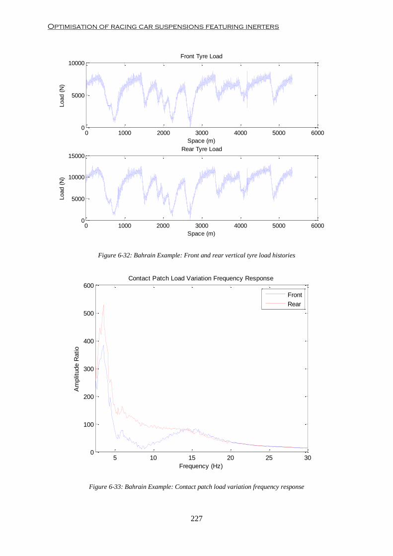
Optimisation of racing car suspensions featuring inerters
227
Figure 6-32: Bahrain Example: Front and rear vertical tyre load histories
Figure 6-33: Bahrain Example: Contact patch load variation frequency response
0 1000 2000 3000 4000 5000 60000
5000
10000Front Tyre Load
Space (m)
Load (
N)
0 1000 2000 3000 4000 5000 60000
5000
10000
15000Rear Tyre Load
Space (m)
Load (
N)
5 10 15 20 25 300
100
200
300
400
500
600Contact Patch Load Variation Frequency Response
Frequency (Hz)
Am
plit
ude R
atio
Front
Rear

Chapter 6- Lap-Time Simulation
228
6.6. Summary
A novel transient lap-time simulation algorithm has been developed in this chapter. The
algorithm uses a multilevel architecture in order to efficiently transcribe the time Optimal
Control problem into a Non-Linear Programming problem. A closed-loop path preview
steering controller has been used to transform the constrained time Optimal Control problem
into an unconstrained one with reduced size. The Non-Linear Programming problem is then
solved by a classical gradient-based Sequential Quadratic Programming solver built in
MATLAB®.
A vehicle model has been also created using a modular modelling approach. The vehicle is
split into subsystems that have been independently modelled. A main vehicle framework has
been then set in order to interconnect the building modules and to produce the overall vehicle
model. This modular modelling approach allows the user to easily interchange, reuse or
update different components without affecting the rest of the model.
The optimisation algorithm has been applied to a case study. A generic racing car with high
downforce levels has been driven along a Bahrain GP Circuit. Discussions with regard to
algorithm efficiency and robustness have been carried out. It was demonstrated that program
framework set-up plays an important role in finding the optimal racing line. Time histories
for different dynamic magnitudes can be obtained and used to analyse the performance and
sensitivity of different vehicle systems into the overall performance of the race car.
In the following chapter, the lap-time simulation virtual tool will be used as decision maker in
a multi-objective suspension optimisation process. The lap-time simulator will be used as key
tool in the analysis of the impact of suspension dynamics in the overall performance of a
racing car.

Optimisation of racing car suspensions featuring inerters
229
7. Suspension Performance Optimization
7.1. Introduction
Suspension systems are a critical part of a racing vehicle. Vehicle suspensions are the only
physical linkage between the tyres and chassis. A critical design consideration for a vehicle
suspension is that they need to offer proper tyre kinematic attitude so that they can react to
the control forces generated at the tyres (acceleration, braking and cornering forces). In
addition, from a purely dynamic point of view, the main goals of a vehicle suspension are:
To keep the tyres in contact with race track.
To resist chassis motions induced by external forces (inertial and aerodynamic
forces).
To control the weight balance across all four tyres under dynamic situations.
The level of accomplishment of these suspension goals will dictate the performance of the
vehicle. Hence, suspension systems must be designed and optimised so that these goals can
be achieved and therefore, maximum vehicle performance can be reached. However, in order
to meet these goals in an efficient and robust way, an optimisation process must be
developed. This chapter presents an objective method capable of optimising a suspension
featuring inerters.
Chapter 7 starts with a formal definition of the suspension optimisation problem as a multi-
objective optimisation problem. The chapter then follows with the definition of the
suspension variables that integrate the optimisation search space and develops a mathematical
expression of the evaluation functions that represent the main dynamic suspension goals
stated above. Moreover, a novel suspension optimisation method based on metamodeling
techniques, multi-objective algorithms and lap-time simulation has been developed. In the
last part of the chapter, this optimisation methodology has been applied to optimise a
conventional suspension and a suspension incorporating inerters. Discussions on the
performance gains obtained from using inerters have been carried out.

Chapter 7- Suspension Performance Optimisation
230
7.2. Definition of the Multi-Objective Suspension Optimisation
Problem
Analytical suspension optimisation based on the use of mathematical optimisation methods
requires firstly an appropriate definition of the optimisation problem. The definition of the
optimisation problem also assists in the selection and development of the most well-suited
optimisation algorithm. As introduced in Chapter 2, the design and optimisation of race car
suspensions must account for several factors. Therefore, a racing suspension system must be
optimised for not only one objective but for several objectives, some of which may conflict
with each other. Hence, a racing car suspension optimisation problem could be defined as a
multi-objective optimisation problem (MOOP). Mathematically, a general MOOP can be
defined as follows (Deb, 2001):
Where x={x1, x2, ... , xn} is the vector of n decision variables
F(x) is the vector of m objective functions
G(x) is the vector of j inequality constraints
H(x) is the vector of k equality constraints
xiL, xiU are the limits of the search space for the i-th decision variable
This formal definition of a general MOOP will assist in the design and development of an
optimisation algorithm that could handle the simultaneous optimisation of several
performance objectives, some of which may conflict with each other, and to obtain an
optimised suspension solution in a robust and efficient manner.
7.3. Definition of the Design Space
The design space or search space, Z, is defined implicitly by the specification of the design
variables z ϵ Z. In a suspension optimisation problem, the design space Z is composed of all

Optimisation of racing car suspensions featuring inerters
231
adjustable suspension parameters such as spring stiffness characteristics, damping
characteristics and inertance values. According to the half car vehicle model developed in
Chapter 5, an initial search space will be composed of the following variables:
Front Suspension Stiffness (N/m) ksF
Rear Suspension Stiffness (N/m) ksR
Front Linearised Damping Coefficient (Ns/m) CsF
Rear Linearised Damping Coefficient (Ns/m) CsF
Front Inertance (kg) bsF
Rear Inertance (kg) bsF
Table 7-1: Definition of Initial Design Space
Anti-roll bar (ARB) stiffness values have been neglected from the design space since the
vehicle model does not account for rolling effects.
Furthermore, a preliminary study has been carried out in order to analyse the role of spring
stiffness in suspension optimisation when considering only the dynamic response of the
vehicle to road irregularities. A simple single-degree-of-freedom (SDOF) system similar to
the one represented in Figure 3-4 without an inerter has been used. Due to its simplicity, an
analytical expression for the amplitude ratio between output and input displacement can be
derived using the same procedure employed in Chapter 3. The final expression of the
amplitude ratio is:
Where H(ω): Output/Input Displacement Amplitude Ratio in frequency domain
X(ω): Body Displacement in frequency domain
Z(ω): Base (Road) Excitation Displacement in frequency domain
k: Spring stiffness in N/m
c: Damping Coefficient in Ns/m
m: Body mass in kg
ω: Angular frequency in rad/s

Chapter 7- Suspension Performance Optimisation
232
Equation (7.2) represents the characteristic behaviour of a SDOF system in the frequency
domain for different spring stiffness values for a constant 0.5 damping ratio (see Figure 7-1).
In general terms, softer springs decrease the natural frequency of the system and reduce the
vibration transmissibility at higher frequencies.
Figure 7-1: SDOF Body Displacement Amplitude Ratio for different k values
However, in order to quantitatively measure the impact of suspension springs in the dynamic
response of the system, a measurement of the vibration transmission from input (road
irregularities) to output (body) is required. A common tool for quantifying this vibration
transmission used in classical vibration dynamics literature is to calculate the root-mean-
square (RMS) of the transmissibility function, in this case, body displacement amplitude
FRF. The RMS of the body displacement FRF expressed in equation (7.1) RMSb can be
obtained as follows:
Where n: number of samples of the function H(ω).
0 20 40 60 80 100 120 140 160 180 2000
0.5
1
1.5Body Displacement Amplitude Ratio Frequency Response
Angular Frequency (rad/sec)
X(w
)/Z
(w)
ks=15000 N/m
ks=30000 N/m
ks=45000 N/m

Optimisation of racing car suspensions featuring inerters
233
Thus, using expression (7.3) and (7.2), an analysis of the variation of stiffness values, k, on
the RMS of the body displacement can be carried out. Figure 7-2 shows the trend of RMS of
the body displacement for different spring values, expressed as ride frequency.
Figure 7-2: Effect of suspension stiffness in the RMS of Body Displacement Amplitude Ratio
It can be observed that body displacement transmissibility decreases monotonically with
softer suspension stiffness. On the limit k → 0, the transmissibility function tends to 0, which
leads to the trivial solution that with no springs between road and body, body displacement
would be completely independent from road excitations. This means that, when optimising
suspension parameters for more complex vehicle models, the optimiser will obtain the softest
spring value within the specified spring stiffness search range as optimal solution. According
to this, front and rear spring stiffnesses can be therefore discarded from the design space and
only damping and inertance values will be considered as input variables to the optimisation
process.
Hence, the optimisation process presented in this research work considers that the selection of
the optimal spring stiffness is dominated by static and steady-state design constraints such as
static deflection, suspension travel, maximum heave, pitch and roll travel under inertial and
0 0.5 1 1.5 2 2.5 3 3.5 4 4.5 50
0.1
0.2
0.3
0.4
0.5
0.6
0.7Effect of suspension stiffness in suspension optimisation
Ride Frequency (Hz)
RM
S o
f B
ody D
ispla
cem
ent
am
plit
ude R
atio

Chapter 7- Suspension Performance Optimisation
234
aerodynamic forces and steady-state roll distribution, which are outside the scope of the
project.
The final search space is therefore composed of front and rear axle damping and inertance
coefficients (see Table 7-2).
Front Linearised Damping Coefficient (Ns/m) CsF
Rear Linearised Damping Coefficient (Ns/m) CsF
Front Inertance (kg) bsF
Rear Inertance (kg) bsF
Table 7-2: Definition of Final Design Space
7.4. Definition of Optimisation Evaluation Criteria
The definition of objective functions J is paramount in any optimisation process. In race car
suspension design and optimisation, objective functions must accurately express the attributes
and goals to be achieved. In Chapter 2, a review of the research literature related to
suspension performance cost function definition was discussed.
In this chapter, a series of objective functions have been defined in order to analyse the
impact of suspension dynamics with respect to the overall performance of the vehicle in order
to produce an optimised race car suspension set-up. As explained in Chapter 5, suspension
dynamics studies are carried out in the frequency domain, due to the nature of the road inputs
(assumed to be random noise functions with zero mean value and standard deviation σ).
Moreover, vehicle vibration modes (Heave, Pitch, Roll and Warp or Articulation) are often
decoupled in order to facilitate the analysis of the dynamic behaviour of the suspension.
The aim of this section is to define functions that represent performance features of the race
car under the action of dynamic road inputs. The following subsections describe the
development of the suspension optimisation performance functions used in this research
work.
7.4.1. Mechanical Grip Cost Function
In racing applications, mechanical grip is known as the maximum friction coefficient that can
be obtained for a particular racing tyre only through the use of mechanical systems, i.e.
excluding aerodynamic effects. There are many factors that affect the generation of
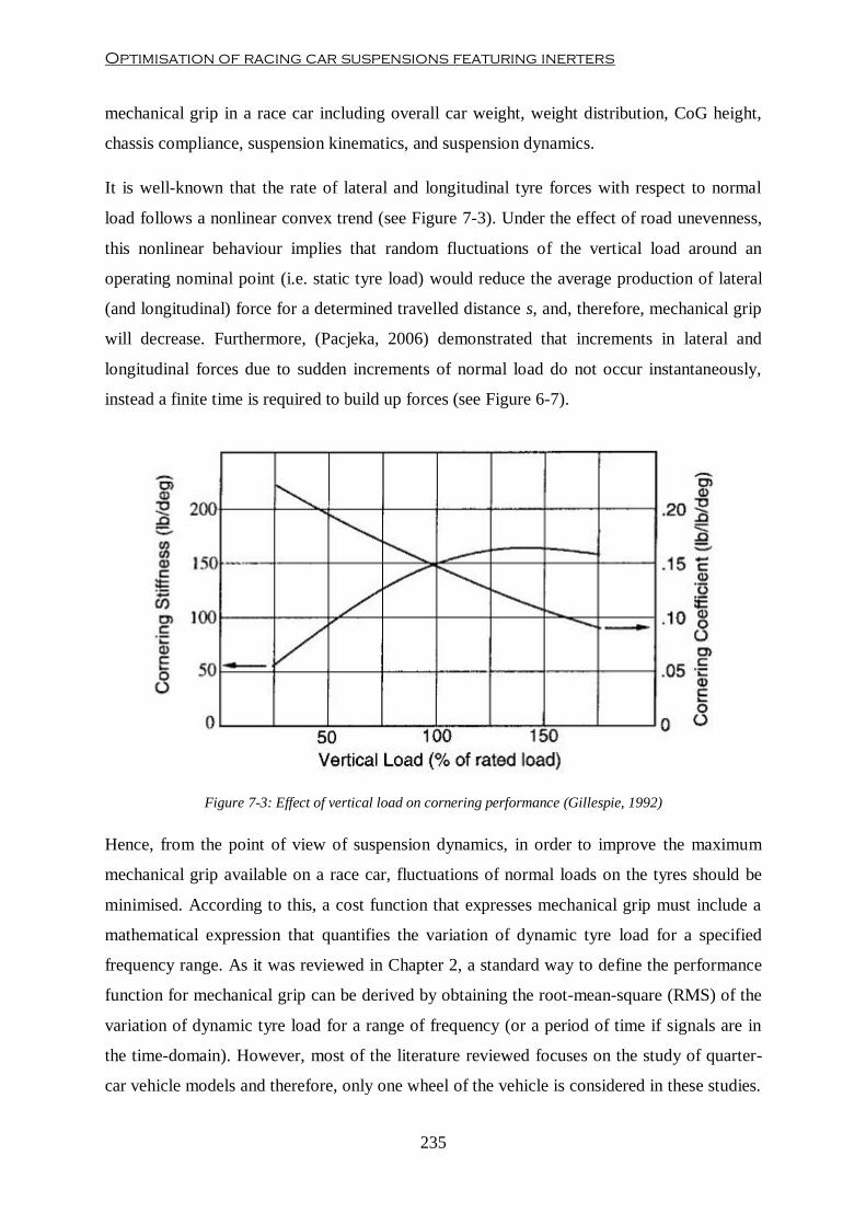
Optimisation of racing car suspensions featuring inerters
235
mechanical grip in a race car including overall car weight, weight distribution, CoG height,
chassis compliance, suspension kinematics, and suspension dynamics.
It is well-known that the rate of lateral and longitudinal tyre forces with respect to normal
load follows a nonlinear convex trend (see Figure 7-3). Under the effect of road unevenness,
this nonlinear behaviour implies that random fluctuations of the vertical load around an
operating nominal point (i.e. static tyre load) would reduce the average production of lateral
(and longitudinal) force for a determined travelled distance s, and, therefore, mechanical grip
will decrease. Furthermore, (Pacjeka, 2006) demonstrated that increments in lateral and
longitudinal forces due to sudden increments of normal load do not occur instantaneously,
instead a finite time is required to build up forces (see Figure 6-7).
Figure 7-3: Effect of vertical load on cornering performance (Gillespie, 1992)
Hence, from the point of view of suspension dynamics, in order to improve the maximum
mechanical grip available on a race car, fluctuations of normal loads on the tyres should be
minimised. According to this, a cost function that expresses mechanical grip must include a
mathematical expression that quantifies the variation of dynamic tyre load for a specified
frequency range. As it was reviewed in Chapter 2, a standard way to define the performance
function for mechanical grip can be derived by obtaining the root-mean-square (RMS) of the
variation of dynamic tyre load for a range of frequency (or a period of time if signals are in
the time-domain). However, most of the literature reviewed focuses on the study of quarter-
car vehicle models and therefore, only one wheel of the vehicle is considered in these studies.

Chapter 7- Suspension Performance Optimisation
236
In this research work, a half-car vehicle suspension model has been used. Therefore, the cost
function for mechanical grip should include the effects of both axles. According to this, the
following mathematical model can be derived:
Where : Mechanical grip performance function for an isolated vibration mode
qHf, qHr: weighting factors for heave mode between front and rear axles and
The introduction of these weighting factors qHf and qHr enables the possibility to bias
optimisation towards one of the axles. This implies that if qHf > qHr, then the optimised
suspension configuration will produce better mechanical grip on the front axle. An inverse
situation would occur when qHf < qHr. If qHf = qHr, the optimisation solver will attempt to
obtain a suspension setting that evenly increases the dynamic mechanical grip available in
both axles.
Furthermore, in real cars, road excitations are exerted at all four wheels and all the vibration
modes are highly coupled. Thus, the overall objective function should include the calculation
of dynamic contact patch load for all the vibration modes. However, as discussed in Chapter
5, the analysis of ride dynamics does not produce representative results of the actual
behaviour of the physical car for the roll vibration mode and, therefore, it was decided to
model the vehicle suspension to consider only heave and pitch vibration modes.. Hence, a
cost function should incorporate contact patch load CPL variation in heave and pitch modes.
According to this, in this research work, a frequency dependent modal weighting function
WF has been developed. The purpose of this function is to weight the contribution of the
different vibration modes to the overall objective function. This weighting function WF has
been developed from simulated track profile data. This profile data has been created as
integrated white noise (IWN) whose PSD profile resembles the one obtained from the swept
sine input signals discussed in Chapter 4. This IWN signal is then considered as the input
experienced by the front axle. The input excitation at the rear axle has been assumed to be the
same as the input at the front axle delayed by the wheelbase in the space domain (see Figure
7-4).

Optimisation of racing car suspensions featuring inerters
237
Figure 7-4: Integrated white noise track profile signal
Assuming a solid rigid chassis, the content of pure heave motion zHeave and pitch motion φPitch
can be obtained as follows:
Where zrF and zrR: vertical road profile at front and rear axles respectively
wb: wheelbase
a: distance from the front axle to the CoG
b: distance from the rear axle to the CoG
Since cost functions are created from frequency domain data, pure heave and pitch motion
are transformed into frequency domain via Fast Fourier Transformation (FFT). Relative
amplitude responses for heave and pitch motions are then obtained to produce modal
weighting functions WF as:
840 860 880 900 920 940 960 980 1000 1020 1040
-8
-6
-4
-2
0
2
4
6
Space (m)
Vert
ical pro
file
(m
m)
Track vertical profile
Front
Rear
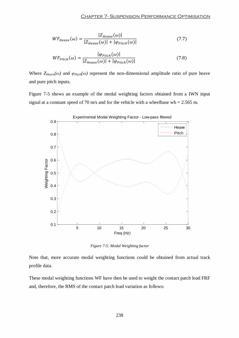
Chapter 7- Suspension Performance Optimisation
238
Where ZHeave(ω) and φPitch(ω) represent the non-dimensional amplitude ratio of pure heave
and pure pitch inputs.
Figure 7-5 shows an example of the modal weighting factors obtained from a IWN input
signal at a constant speed of 70 m/s and for the vehicle with a wheelbase wb = 2.565 m.
Figure 7-5: Modal Weighting factor
Note that, more accurate modal weighting functions could be obtained from actual track
profile data.
These modal weighting functions WF have then be used to weight the contact patch load FRF
and, therefore, the RMS of the contact patch load variation as follows:
5 10 15 20 25 300.1
0.2
0.3
0.4
0.5
0.6
0.7
0.8
0.9Experimental Modal Weighting Factor - Low-pass filtered
Freq (Hz)
Weig
hting F
acto
r
Heave
Pitch
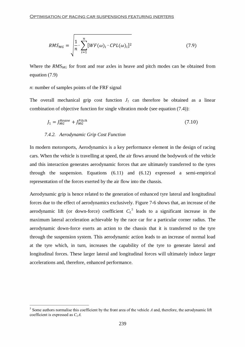
Optimisation of racing car suspensions featuring inerters
239
Where the RMSMG for front and rear axles in heave and pitch modes can be obtained from
equation (7.9)
n: number of samples points of the FRF signal
The overall mechanical grip cost function J1 can therefore be obtained as a linear
combination of objective function for single vibration mode (see equation (7.4)):
7.4.2. Aerodynamic Grip Cost Function
In modern motorsports, Aerodynamics is a key performance element in the design of racing
cars. When the vehicle is travelling at speed, the air flows around the bodywork of the vehicle
and this interaction generates aerodynamic forces that are ultimately transferred to the tyres
through the suspension. Equations (6.11) and (6.12) expressed a semi-empirical
representation of the forces exerted by the air flow into the chassis.
Aerodynamic grip is hence related to the generation of enhanced tyre lateral and longitudinal
forces due to the effect of aerodynamics exclusively. Figure 7-6 shows that, an increase of the
aerodynamic lift (or down-force) coefficient CL5 leads to a significant increase in the
maximum lateral acceleration achievable by the race car for a particular corner radius. The
aerodynamic down-force exerts an action to the chassis that it is transferred to the tyre
through the suspension system. This aerodynamic action leads to an increase of normal load
at the tyre which, in turn, increases the capability of the tyre to generate lateral and
longitudinal forces. These larger lateral and longitudinal forces will ultimately induce larger
accelerations and, therefore, enhanced performance.
5 Some authors normalise this coefficient by the front area of the vehicle A and, therefore, the aerodynamic lift
coefficient is expressed as CLA.

Chapter 7- Suspension Performance Optimisation
240
Figure 7-6: Effect of aerodynamics in the cornering performance of a race car (Dominy, 1992)
Although the absolute aerodynamic performance depends mostly in the design of the
bodywork, interaction between suspension dynamics and aerodynamics is also an important
component in the overall performance of the vehicle. As showed in Chapter 6, the
performance of an aero package is highly sensitive to variations in ride height and attitude. It
is common practice in the industry that aero-maps are expressed as functions of front and rear
ride heights rather than ride height at the CoG and attitude (see Figure 6-8). In Chapter 4,
front and rear ride heights RH were defined as the difference between the displacement of the
sprung mass xs and the input displacement xinput (see equation (4.22)). According to aero-
maps showed in Figure 6-8, the main aim of the suspension system in high aerodynamic
performance cars is to reduce dynamic variations of ride height so that maximum generation
of down-force can be achieved.
Hence, an aerodynamic grip cost function for suspension optimisation must express this
interaction between Aerodynamics and suspension dynamic effects. In this research work, the
aerodynamic suspension performance is quantified in terms of the dynamic ride height
variation. As with the mechanical grip, the root mean square (RMS) function is the most
suited mathematical function to quantify dynamic ride height variations. Front and rear axle
contributions have been equally accounted for in the design of the objective. The weighting
factor developed in the previous section has been also used in this cost function to account for
heave and pitch motions. Thus, the cost function can be expressed as follows:

Optimisation of racing car suspensions featuring inerters
241
Where J2: Overall aerodynamic grip objective function
: aerodynamic objective function for a single vibration mode where
Equation (7.13) applies for the calculation of RH for front and rear axles in heave and pitch
modes
WF: Frequency based modal weighting function
RH(ω): dynamic ride height variation FRF
n: number of samples points of the FRF signal
Furthermore, since the aerodynamic longitudinal force distribution is ride height dependent,
the cost function defined in equation (7.11) accounts also for aerodynamic balance effects.
Minimisation of dynamic ride height variations will lead to reduction of the variation of the
aero distribution and therefore to an improvement of the aerodynamic balance.
7.4.3. Mechanical balance Cost Function
Mechanical balance is another important feature in racing cars. Mechanical balance refers to
the amount of grip produced at each axle. A perfectly balanced car would produce lateral axle
forces so that the resultant moment around the yaw axis is always zero under steady-state
cornering. If the front axle produces less lateral force than the rear axle, the car experiences
an understeering situation and is unable to follow the ideal racing line. If the rear axle
produces less lateral force than the front axle, then the vehicle experiences an oversteering
situation in which the vehicle becomes unstable.
The steady-state mechanical balance of a vehicle depends mostly on weight distribution, tyre
cornering stiffnesses and slip angles. However, Mashadi & Crolla (2005) showed that the

Chapter 7- Suspension Performance Optimisation
242
understeering characteristic of a vehicle under relatively high lateral accelerations is
dramatically affected by the effect of road unevenness.
Figure 7-7: Understeering characteristic under different road surfaces (Mashadi & Crolla, 2005)
Hence, in this research work, a cost function that expresses the effect of suspension dynamics
on the understeer – oversteer characteristic of a vehicle has been developed.
Assuming a steady-state understeer gradient dictated by the design of the chassis and the
selection of the tyres, the dynamic understeer characteristic of a vehicle can be influenced by
road excitation through the suspension system. Road irregularities generate dynamic normal
load changes at the tyre contact patch. If variations of normal load are different for each axle,
the weight distribution under dynamic loads will drift from static weight distribution and
therefore this will change the balance of the car. According to this, an expression of the
dynamic weight distribution WDist_Dyn was defined in Chapter 4 (see equation (4.23)).
Optimisation of racing car suspensions featuring inerters
243
From this expression of dynamic weight distribution WDist_Dyn, a longitudinal deviation of
the position of the dynamic CoG with respect to the static CoG location can be defined as:
Where ECoG(ω): FRF of deviation of dynamic CoG from static CoG longitudinal location. As
with the previous cost functions, this magnitude can be obtained in both heave and pitch
modes
wb: wheelbase
a: distance from static CoG to front axle
As with the rest of the objective functions, the RMS of ECoG(ω) can be obtained in order to
quantify the variation of the position of the dynamic CoG with respect to the static CoG as:
The mechanical balance objective function J3 can be obtained by combining the RMSBalance
for heave and pitch modes.
7.5. Development of the Optimization Methodology
The main goal of developing a validated vehicle suspension model is that it can then be used
to perform analyses in a virtual environment with high levels of confidence. Moreover,
results drawn by simulation modelling can be directly applied to the physical car.
In this research work, the validated vehicle model is used, in combination with the
performance based objective functions defined in section 7.4, as an input into a suspension
optimisation problem in a virtual environment. This process allows an optimal suspension
setup to be obtained much more efficiently and robustly than when carrying out experimental
testing on a rig facility or a race track.

Chapter 7- Suspension Performance Optimisation
244
Figure 7-8 shows the optimisation method proposed in this thesis in order to obtain an
optimised suspension setup. The following sections provide a detailed explanation of the
different stages of this suspension optimisation.
Figure 7-8: Proposed suspension optimisation process layout
Validated
Vehicle Model
(Ch. 5)
Search Space
(Ch. 7)
Cost Functions
(Ch. 7)
Optimisation
Engine
(Ch. 7)
Optimised
Suspension
Setup
Lap-time
Simulator
(Ch. 6)
Metamodelling
technique
Surrogate
model
Multi-objective Evolutionary
Algorithm
Pareto Optimal
Front
Decision Making
Process
Single optimal
solution

Optimisation of racing car suspensions featuring inerters
245
7.5.1. Surrogate Modelling using Kriging Method
A vehicle suspension system can be defined as a dynamic model composed of a series of
differential equations that describe the motion of system as a function of time t. Due to its
complexity, the solution of the differential equations that describe a vehicle suspension model
can only be obtained by numerical techniques (e.g. Runge-Kutta method). These numerical
techniques are often quite computationally expensive.
As defined in the previous section, the definition of the vehicle suspension performance
metrics requires the solution of the dynamic system via numerical integration methods. Since
the optimisation tool must evaluate these performance cost functions several times (hundreds
or even thousands of times) in order to find an optimal solution, the simulation time of the
dynamic system will exhibit a great impact in the overall efficiency of the optimisation tool.
In the present thesis, a surrogate modelling technique has been introduced in order to
minimise the simulation time of the optimisation tool. Surrogate or metamodelling techniques
were first introduced in Chapter 2. These techniques use mathematical and statistical methods
to relate model input variables to output variables without the requirement of solving the set
of differential equations that describe the behaviour of a particular dynamic system.
Metamodels or surrogate models approximate the solution of the cost functions to a
mathematical surface dependent only on the input parameters. A surrogate model will
therefore substitute the actual dynamic model without any loss of information provided that
the surrogate model can replicate with good fidelity the dynamic behaviour of the actual
system. Hence, by using surrogate models, numerical integration of the dynamic model is no
longer required due to the fact that the variables defined in the search space Z are related to
the performance cost functions through algebraic equations. Figure 7-9 summarises
graphically the advantages of using surrogate modelling for the evaluation of cost functions.

Chapter 7- Suspension Performance Optimisation
246
Figure 7-9: Optimisation cost function evaluation through actual dynamic model (upper) and surrogate model
(lower)
Regardless of the method utilised to generate approximate models, a finite number of sample
points N within the search space must be selected. These sample points will be used to create
the fitting between the surrogate and original model. In order to efficiently select these points
within the search space, a design of experiments (DoE) must be undertaken. Different DoE
techniques can be found in literature. In this research work, a Space-filling technique called
Latin Hypercube has been used to spread the sample points across the search space.
There are several approaches available in literature for constructing surrogate models (see
Chapter 2). In the present thesis, a Kriging metamodelling technique has been used to
construct surrogate models for cost functions due to the successful application of this
technique in previous studies (Simpson, 1998; Simpson, et al., 2001). Kriging method is a
combined model that can be defined as follows:
Where f(x) represents a global approximation of the original function and it is expressed as a
polynomial model
Numerical
Integration z J
z J
Actual dynamic model
Surrogate model

Optimisation of racing car suspensions featuring inerters
247
Z(x) is expressed as a stochastic function that represents localised deviations in between data
samples
x represents the input variables
y(x) represents the output of the surrogate model
The polynomial function f(x) is commonly reduced to a zero-order polynomial function or
constant term β (Jin, 2005). The stochastic function Z(x) is characterised by zero mean,
variance σ2 and non-zero covariance that can be defined as follows:
Where R is a NxN symmetric correlation matrix composed of ones along the main diagonal
and R(xi,x
j) is a correlation function between the sample data points i and j. The correlation
function can be selected by the user. In this research work a Gaussian correlation function has
been used. The Gaussian correlation function can be expressed as:
Where θk are the unknown correlation parameters used to fit the surrogate model and ns
represents the dimension of the design space x.
In order to test the accuracy of the surrogate model, a simple study has been carried out. A
SDOF system has been used to evaluate the performance of a Kriging model. The design
space of the analysis is composed by spring stiffness ks and damping cs values. Moreover,
boundaries to the design space must be set. In this case study, ks will range from 50 N/mm to
500 N/mm and cs will range from damping ratio from 800 Ns/m to 15000 Ns/m. Two simple
cost functions have been defined: the RMS of the normalised body acceleration and the RMS
of the normalised ride height. Both cost functions have been calculated from frequency
domain data.

Chapter 7- Suspension Performance Optimisation
248
Where x(ω) and ẍ(ω) are the body displacement and acceleration in frequency domain
z(ω) and (ω) are the input displacement and acceleration in frequency domain.
A Kriging surrogate model is constructed from the original model using 50 sample points
selected through a Latin Hypercube sampling data technique using the built-in MATLAB®
function lhsdesign (The MathWorks Inc., 2012). Once the metamodel has been built, a set of
evaluation points has been selected to evaluate the accuracy of the metamodel with respect to
the original model. For brevity at this stage, the evaluation points have been selected such
that the damping ratio of the system is always 0.7. Figure 7-10 to Figure 7-12 show the
accuracy of the metamodel with respect to the original model. As can be observed, estimation
errors are typically below 0.5% across the design space. The estimation error grows to values
below 5% at the lower bound of the design space. This suggests that the metamodelling can
reproduce the behaviour of the original model with excellent accuracy in regions inside the
DoE space and this level of accuracy reduces in regions near the limits of the DoE space.
Figure 7-10: Evaluation of the performance of the metamodel in predicting cost function J1
0 0.5 1 1.5 2 2.5 3 3.5 4 4.5 5
x 105
0.58
0.6
0.62
0.64
0.66
0.68
0.7
0.72
0.74
Spring Stiffness (N/m)
J1
Evaluation of J1 for original and metamodel
Original
Metamodel
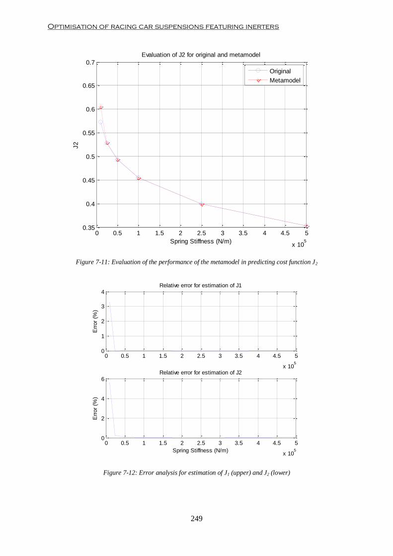
Optimisation of racing car suspensions featuring inerters
249
Figure 7-11: Evaluation of the performance of the metamodel in predicting cost function J2
Figure 7-12: Error analysis for estimation of J1 (upper) and J2 (lower)
0 0.5 1 1.5 2 2.5 3 3.5 4 4.5 5
x 105
0.35
0.4
0.45
0.5
0.55
0.6
0.65
0.7
Spring Stiffness (N/m)
J2
Evaluation of J2 for original and metamodel
Original
Metamodel
0 0.5 1 1.5 2 2.5 3 3.5 4 4.5 5
x 105
0
1
2
3
4
Err
or
(%)
Relative error for estimation of J1
0 0.5 1 1.5 2 2.5 3 3.5 4 4.5 5
x 105
0
2
4
6
Spring Stiffness (N/m)
Err
or
(%)
Relative error for estimation of J2

Chapter 7- Suspension Performance Optimisation
250
This Kriging technique will now be applied to a more complex case. As explained previously,
the evaluation the objective functions developed in section 7.4 requires the numerical
integration of the vehicle suspension model developed in Chapter 5. Thus, Kriging
metamodelling technique will be used to relate input variables (see section 7.3) to the cost
function without the need of the dynamic system.
As explained earlier in this section, a number of sample points must be obtained from the
original model in order to construct the surrogate model. The number of sample points used
to construct surrogate models affects the accuracy of the metamodel and the construction
time. A compromise between accuracy and construction time must be reached. In the present
research work, it was found that n=80 sample points for objectives J1 and J2 and n=120 for
objective J3 produced good results in terms of computational time and quality of the
metamodel created. 50 analysis points have been randomly selected from the DoE space and
objective functions have been evaluated from both the original and the metamodels. Relative
errors have been calculated for each point. Table 7-3 summarises the average relative errors
and the maximum error obtained for each objective function. As results show, the Kriging
metamodelling technique has been able to produce highly accurate surrogate models, with
average errors below 0.5 % for objectives J1 and J2 and below 2 % for objective J3. Maximum
errors have been also recorded for each objective function: meanwhile maximum errors for J1
and J2 are about 1 %, J3 presents a maximum error of about 5.5 %. As it happened with the
simple case study, this error has been obtained for a point lying in a region close to the limits
of the DoE space. Thus, in order to avoid errors over 5 %, optimisation search space will
contained within the limits of the DoE space.
Average Error Maximum Error
Objective 1 0.33 % 0.96 %
Objective 2 0.31 % 1.05 %
Objective 3 1.77 % 5.76 %
Table 7-3: Analysis of accuracy of Kriging metamodel for each cost function
Table 7-4 compares construction and simulation times of original and surrogate models for
different batches of analysis points Nanalysis. Although simulation time required to evaluate the
objectives has been highly reduced with respect to the original model, the additional time
required to construct the surrogate models indicates that surrogate models will only be more
computationally efficient when large number of objective evaluations are required.

Optimisation of racing car suspensions featuring inerters
251
Model Construction
Time
Simulation time
Nanalysis=25 Nanalysis=50 Nanalysis=100
Original - 118 secs 237 secs 466 secs
Kriging surrogate 362 secs 0.005 secs 0.011 secs 0.018 secs
Table 7-4: Summary of computational time of original and metamodel for batch simulation
Furthermore, a multiobjective optimisation process has been carried out for both the original
and the surrogate cost functions. Although the optimisation solver used in this case study will
be described in the following section, it has been used to demonstrate the efficiency and
accuracy of the Kriging method. The main optimisation parameters set for this case study are:
Initial population: 50 individuals
Maximum number of generations: 25
Moreover, the hybrid algorithm has been set in sequential mode, i.e. the results of the MOEA
are then fed into the local SQP algorithm. Figure 7-13 shows the results of the suspension
optimisation. Note that for clarity only mechanical grip (Objective 1) and aerodynamic grip
(Objective 2) performance metrics have been plotted.
Figure 7-13 show the estimation of the Pareto optimal front. As it can be observed, the
prediction of the Pareto optimal front obtained via the metamodel presents a good correlation
with respect to the Pareto front obtained via the original. Although the scattered points do not
fall into exactly the same places, the trend is very similar. A maximum error of 1.5% has
been calculated in the estimation of the Pareto front.
In addition to this, the computation times for optimisation via original and metamodels have
been recorded. Table 7-5 summarises the total time required to obtain the solution to the
optimisation problem shown in Figure 7-13. Although some time is required to build the
surrogate models, the actual optimisation time has been highly reduced with respect to the
original model. Hence, by the use of a Kriging surrogate model, the overall optimisation
process runs over 15 times faster than the original model.

Chapter 7- Suspension Performance Optimisation
252
Figure 7-13: Cost function comparison between metamodel and original vehicle suspension model
Model Construction Time Optimisation Time Total Time
Original - 5988 secs 5988 secs
Kriging surrogate 362 secs 13 secs 375 secs
Table 7-5: Summary of computational time of original and metamodel for optimisation
7.5.2. Multi-Objective Algorithm
Racing car suspensions present an important role in the performance of the vehicle due to the
interaction with tyres and aerodynamics. Furthermore, due to the multiple goals a racing car
suspension must achieve in order to maximise the performance of the vehicle, in section 7.2,
the suspension optimisation problem was defined as a Multi-Objective Optimisation problem
(MOOP). In this section, an optimisation tool capable of solving suspension MOOP is
presented.
This MOOP requires a solution method capable of optimising several conflicting objective
functions simultaneously. Several optimisation methods have already been reviewed in
Chapter 2. Multi-objective Evolutionary Algorithms (MOEAs) are well-suited for obtaining a
set of solutions when several conflicting objectives are to be optimised. A vast variety of
MOEAs can be found in literature. In this research work, an elitist non-dominated sorting
140 160 180 200 220 240 260 28018.5
19
19.5
20
20.5
21
21.5
22
Objective 1
Obje
ctive 2
Metamodel
Real model

Optimisation of racing car suspensions featuring inerters
253
genetic algorithm (NSGA-II) has been selected as core optimisation method due to the
increased computational efficiency and enhanced ability of finding the true Pareto optimal
front over other MOEAs (Deb, et al., 2002).
Although it is outside the scope of this thesis to describe in detail the working principle of
MOEAs, the main features of the NSGA-II optimisation tool used in this research work can
be summarised as follows:
It is a rank-based EA: individuals in the population are ranked according to the
fitness score and sorted into non-dominated layers.
It is an elitist EA: A sub-set of the best individuals of each generation is transferred
to the following generation unaltered.
It uses a crowded comparison operator in order to maintain diversity along the Pareto
optimal line.
A Tournament selection method has been used in the selection stage.
A simulated binary crossover (SBX) operator has been used in the mating stage.
A polynomial mutation technique has been used in the mutation stage.
Moreover, EAs are unlikely to find the true Pareto optimal solution due to the stochastic
nature of their search engine. Hybrid techniques can therefore be used to overcome this
problem (Deb & Goel, 2001). By using this hybrid technique, the results of the MOEA are
fed into a local convergence search method, generally a gradient-based algorithm, so that true
Pareto optimal solutions can be obtained. This hybrid algorithm combines the ability of
finding a near true Pareto optimal front in only one optimisation run with the strong local
convergence of gradient-based algorithms. In this research thesis, the NSGA-II has been
coupled with a Sequential Quadratic Programming (SQP) algorithm.
As depicted in Figure 7-13, due to the conflicting nature of the objective functions, the
outcome of this optimisation process is a set of non-dominated optimised suspension setups
(Pareto Optimal front). This means that the suspension optimisation problem is
underdetermined, i.e. there are several solutions to the problem. However, since current
racing regulations do not allow any suspension tuning during racing events, a single solution
must be selected among the Pareto front. In order to select an optimal solution from the
Pareto front, additional information of the vehicle is required. This information can be
obtained from different sources, from CAE simulation tools to race engineer´s experience.
Chapter 7- Suspension Performance Optimisation
254
The process of acquiring information and using it to find a single optimum is known as
decision making process (Deb, 2001). In this research work, a novel decision making
technique based of lap-time simulation has been developed. The following section describes
the process by which a LTS can be used to objectively obtain a particular solution from the
Pareto set.
7.5.3. Decision Making Process via the use of Lap-time simulation
The process described above provides a set of optimal non-dominated solutions. Each of the
solutions contained in this optimal set offers no improvement in all objectives functions
simultaneously. Thus, a decision making process must be enabled in order to select a single-
point solution from the optimal set. The decision making process must be fed with additional
information that has not been already contained in the mainstream of the optimisation
process. This decision making process often contains a certain level of subjective information
and it is not well defined and documented, e.g. a race engineer may use his experience and
driver feedback to act as the decision maker of the suspension optimisation process.
The aim of the research process is to define an objective decision maker based in data
obtained from simulation techniques. In order to account for all the additional information not
contained in the suspension optimisation process, the LTS developed in Chapter 6 will be
used as decision maker for the optimisation process.
The ultimate goal of any racing car is to complete a lap in shortest time possible. Hence, the
decision maker must find a particular suspension setup within the Pareto set that optimises
the final lap time. The approach in this research work is to cluster the solutions of the Pareto
front into a number of finite solutions and a direct search algorithm is used to find the single
optimal solution: each suspension setup from the clustered set is fed into the LTS and a lap
time is obtained. The suspension setup that minimises lap time on a particular circuit will be
the single optimal solution.

Optimisation of racing car suspensions featuring inerters
255
Figure 7-14: Decision Making Process
LTS compiles data from different systems that integrate the vehicle and environmental
factors to analyse the ultimate performance of a race car on a particular car. Depending on the
level of LTS complexity, more information not strictly contained in earlier stages of the
optimisation process (track surface, track layout, aeromaps, tyre maps, suspension
kinematics, etc.) could be used to find the final optimal solution. In addition to this, LTS
allows the analysis of the impact of suspension dynamics in other vehicle subsystems such as
steering, suspension kinematics, aerodynamics, etc.
The next section uses the optimisation process explained in this section in order to obtain an
optimised suspension solution.
7.6. Case Study
In this section, the optimisation process depicted in Figure 7-8 and described in previous
sections has been applied to a practical case study. Two vehicle suspension layouts have been
analysed: a conventional suspension layout and a suspension featuring real inerters. In the
first sub-section, the main parameters required to set up the optimisation process are defined;
and in the second sub-section, results of the optimisation process for each suspension layout
are presented and discussed.
7.6.1. Optimisation Process Set-up
Recalling Figure 7-8, the inputs of the optimisation process are:
Vehicle suspension model
Optimisation search space
Performance cost functions
Multiobjective
Optimisation
Data
Clustering
Lap-time
Simulation
Decision
Making

Chapter 7- Suspension Performance Optimisation
256
First, the validated vehicle suspension model developed in Chapter 5 has been used as input
to the optimisation process (see Figure 5-21). This model can be featured to analyse both
conventional suspensions and suspensions with inerters. In the case of a conventional layout,
the inerter model branch can be eliminated by setting inerter and damper values to 0 (open-
circuit) and stiffness values to 1 (short-circuit).
Secondly, the optimisation search space has been composed by front and rear axle damper
and inerter values (see section 7.3). In the case of conventional suspension layout, the search
space reduces only to 2 variables: front and rear damping coefficients. The range of the
design space can be summarised in the following table:
Lower Bound Upper Bound
Front damping (Ns/m) 850 3500
Rear damping (Ns/m) 850 3500
Front inertance (kg) 1 40
Rear inertance (kg) 1 40
Table 7-6: Limits of the optimisation design space
The limits have been set so that a vast variety of suspension settings could be analysed by the
optimiser. Damping limits cover from a lightly damped suspension setting (ζ≈0.25) to a
heavily damped suspension setting (ζ≈1.2). Accordingly, inertance values have been set to
range from an inertance-to-weight ratio of 0.01 to an inertance-to-weight ratio of about 0.75.
Note that, in the case of conventional suspension layout, front and rear inertance will be set to
0 and front and rear damping limits will remain unchanged.
Thirdly, cost functions for mechanical grip, aerodynamic grip and mechanical balance (see
section 7.4) have been used as target in the optimisation process for both suspension cases.
As explained in section 7.5, metamodels for all three performance cost functions have been
built. These surrogate models can be effectively used in substitution for the original objective
metrics. In order to improve the accuracy of the surrogate model within the range of the
optimisation design space (see Table 7-6), larger limits have been defined to construct the
DoE space. The limits of the DoE space can be summarised in Table 7-7.

Optimisation of racing car suspensions featuring inerters
257
Lower Bound Upper Bound
Front damping (Ns/m) 750 4000
Rear damping (Ns/m) 750 4000
Front inertance (kg) 0 45
Rear inertance (kg) 0 45
Table 7-7: Limits of the DoE space
Once metamodels for all cost functions have been successfully created, next step is to run the
hybrid multi-objective optimiser described in section 7.5. Table 7-8 shows the main
parameters required to set the MOEA.
Population size 100
Generations 100
Elite fraction 10 %
Crossover function 80 %
Table 7-8: MOEA setting parameters
Solutions of the multi-objective optimisation stage are then clustered into a limited number of
discrete solutions. In this case study, it has been decided that, for each suspension layout, 10
solution points will be created and uniformly scattered across the Pareto Optimal surface.
According to the level of detail the user is trying to achieve, more points could be selected.
These solution points will then be fed into the decision making process where each
suspension layout will be tested on the LTS developed in Chapter 6. The LTS has been
determined according to the following points:
Only suspension parameters will be tuned during the decision making process.
The vehicle model presents the same parameterisation as in the case study presented
in Chapter 6.
The Bahrain International GP Circuit has been used as race track.
The parameters required to set up the lap-time simulation remain unchanged (see
Chapter 6).
The following section presents and discusses the results of the optimisation process.

Chapter 7- Suspension Performance Optimisation
258
7.6.2. Optimisation results and discussions
The first gateway of the optimisation process is the solution of the multi-objective stage.
After the application of the MO optimiser, a set of non-dominated optimal solutions has been
obtained for a conventional layout (L1) and for a suspension with inerter layout (L2). The
results of the multi-objective optimisation stage are shown in Figure 7-15 and Figure 7-16.
Figure 7-15 shows the 3D Pareto Optimal surface generated by the interaction of the three
objective metrics. As can be observed, the shape and location of the optimised surface drawn
for each suspension layout are quite different: on one hand, the cloud of optimal solutions is
located in different regions within the objective space. Due to the way in which the objective
functions have been defined (minimisation cost functions), solution points closer to the origin
represent optimised solutions with respect to points further away for the origin. In this case
study, L1 and L2 clouds intersect each other, which indicate that one layout will offer
enhanced suspension performance on a particular objective with respect to the other layout.
On the other hand, both layouts present a convex Pareto surface, which means that the
performance functions are conflicting between each other. However, the Pareto surface for
layout L2 is sparser than for L1. Although, the shape of the Pareto contour is similar in a J1-
J2 2D view (see Figure 7-16), the sparsity is quite different in the other to views. This
suggests the suspension layout could alter the interaction between objectives.
Figure 7-16 presents in more detail the particular one-to-one interactions between objectives
for both suspension layouts. Arrows depict the principal direction of increasing damping and
inertance values. As the graphs demonstrate, for both layouts, there is a principal conflicting
interaction between mechanical grip J1 and aerodynamic grip J2 observable for both layouts.
However, some differences can be noticed between suspension layout optimisation results:
firstly, optimisation with suspension layout L1 offers improved mechanical grip solutions
with respect to layout L2. The reason for this is that inerters induce an increase in dynamic
tyre load variations at high frequencies due to a less controlled hub vibration mode,
especially with low damping configurations. Secondly, as damping increases, the use of
inerters represents an improvement over conventional suspensions: high damping coefficients
can cause suspension locking-up (i.e. negligible relative motion between sprung and
unsprung masses) and therefore this effect induces an uncontrolled tyre vibration mode.
Inerters reduce the effective damping ratio (see Chapter 3) and enhance the control of the tyre
mode. Furthermore, the combined use of high damping and inertance produces a sensible
improvement in aerodynamic grip.

Optimisation of racing car suspensions featuring inerters
259
Figure 7-15: Suspension multiobjective optimisation results – 3D Plot
140160
180200
220240
260280
18
20
22
24
26
60
80
100
120
140
160
180
200
220
J1
Multiobjective Optimisation Results - 3D plot
J2
J 3
with Inerter
Conventional

Chapter 7- Suspension Performance Optimisation
260
Figure 7-16: Suspension multiobjective optimisation results – 2D plots
The set of optimal suspension presented in the previous figures will be now used as input
decision making process. As explained previously, the Pareto surface must be clustered into a
reduced number solution points. In this particular case study, 10 uniformly distributed
solution points have been selected for each layout. Figure 7-18 and Figure 7-17 show
graphically the distribution of the selected solution points in the objective space for L1 and
L2 suspension layouts respectively. Table 7-10 and Table 7-9 relate each solution point
selected with a determined suspension setting.
↑cs, bs ↑cs, bs
↑cs, bs

Optimisation of racing car suspensions featuring inerters
261
Figure 7-17: Clustered results for MO results – Conventional suspension
Solution
point
Front damping
(Ns/m)
Rear damping
(Ns/m)
1 909 1208
2 1010 1420
3 1067 1516
4 1301 1581
5 1449 1741
6 1845 1523
7 1810 2008
8 1937 2251
9 2465 2218
10 2826 2345
Table 7-9: Summary of clustered optimised suspension settings – Conventional suspension
140
150
160
170
180
190
20
21
22
23
24
2560
80
100
120
140
160
180
200
220
J1
J2
J 3
MOOP results
Clustered results

Chapter 7- Suspension Performance Optimisation
262
Figure 7-18: Clustered results for MO results – Suspension featuring inerters
Solution
point
Front damping
(Ns/m)
Rear damping
(Ns/m)
Front inertance
(kg)
Rear inertance
(kg)
1 976 1272 3.8 4.7
2 1423 1228 6.6 1.3
3 1872 1229 9.8 1.5
4 2062 1489 10.5 4.4
5 2091 1687 7.6 10.2
6 2238 1730 10.8 13.1
7 2814 2009 16.6 13.6
8 2822 2307 18.1 23.8
9 2814 2353 22.1 28.9
10 2863 2752 26.6 36.3
Table 7-10: Summary of clustered optimised suspension settings – Suspension featuring inerters
Finally, the last stage in the optimisation process is to set each suspension variant in the
virtual vehicle model and perform the lap-time simulation. The process has been repeated for
both suspension layouts and optimal lap time has been recorded for each test run. Table 7-11
summarises the lap time recorded for each suspension variant.
140160
180200
220240
260280
18
19
20
21
22
23100
120
140
160
180
200
220
J1
J2
J 3
MOOP results
Clustered results
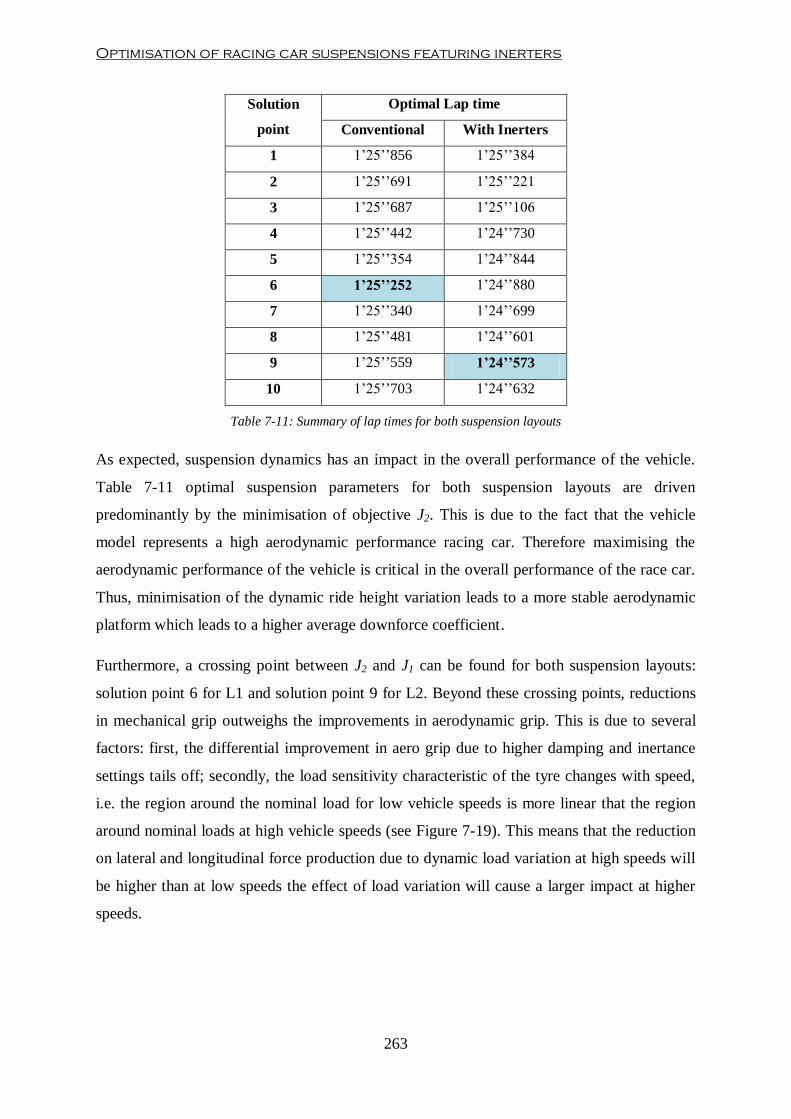
Optimisation of racing car suspensions featuring inerters
263
Solution
point
Optimal Lap time
Conventional With Inerters
1 1’25’’856 1’25’’384
2 1’25’’691 1’25’’221
3 1’25’’687 1’25’’106
4 1’25’’442 1’24’’730
5 1’25’’354 1’24’’844
6 1’25’’252 1’24’’880
7 1’25’’340 1’24’’699
8 1’25’’481 1’24’’601
9 1’25’’559 1’24’’573
10 1’25’’703 1’24’’632
Table 7-11: Summary of lap times for both suspension layouts
As expected, suspension dynamics has an impact in the overall performance of the vehicle.
Table 7-11 optimal suspension parameters for both suspension layouts are driven
predominantly by the minimisation of objective J2. This is due to the fact that the vehicle
model represents a high aerodynamic performance racing car. Therefore maximising the
aerodynamic performance of the vehicle is critical in the overall performance of the race car.
Thus, minimisation of the dynamic ride height variation leads to a more stable aerodynamic
platform which leads to a higher average downforce coefficient.
Furthermore, a crossing point between J2 and J1 can be found for both suspension layouts:
solution point 6 for L1 and solution point 9 for L2. Beyond these crossing points, reductions
in mechanical grip outweighs the improvements in aerodynamic grip. This is due to several
factors: first, the differential improvement in aero grip due to higher damping and inertance
settings tails off; secondly, the load sensitivity characteristic of the tyre changes with speed,
i.e. the region around the nominal load for low vehicle speeds is more linear that the region
around nominal loads at high vehicle speeds (see Figure 7-19). This means that the reduction
on lateral and longitudinal force production due to dynamic load variation at high speeds will
be higher than at low speeds the effect of load variation will cause a larger impact at higher
speeds.

Chapter 7- Suspension Performance Optimisation
264
Figure 7-19: Difference in load sensitivity around
Moreover, the effects of mechanical balance can be noticed in lap times obtained for layout
L2. Suspension settings 5 and 6 produce large values of J3, i.e. poor balanced suspension.
Even though, the aero grip has been improved with respect to previous suspension settings (3
and 4 suspension settings), this poorer mechanical balance between front and rear axle causes
a slower lap times.
Finally, lap times obtained for layouts L1 and L2 must be compared. Table 7-11 shows that
the suspension setting featuring inerters consistently achieves improvements in lap time with
respect to the conventional suspension layout. This is due to the increased aerodynamic grip
obtained by suspension layout 2 with respect to layout 1. Furthermore, in general suspension
layout L2 achieves better mechanical balance than L1. Figure 7-20 and Figure 7-21 compare
a section of the lap-time simulation carried out for the best L1 and L2 suspension
configurations (see Table 7-11). Figure 7-20 shows that race car L2 can take a tighter racing
line around turn 4 than L1 and the driver need not slow down so much to take the corner (see
Figure 7-21) due to the increase in aerodynamic grip and mechanical balance provided by the
suspension featuring inerters.
0.75 0.8 0.85 0.9 0.95 1 1.05 1.1 1.15 1.2 1.250.75
0.8
0.85
0.9
0.95
1
1.05
1.1
1.15
1.2
1.25
Normalised vertical load
Norm
alis
ed late
ral fo
rce
Load sensititivy characteristic for different nominal loads (Fz0)
Fz0 = 2000 N
Fz0 = 7000 N
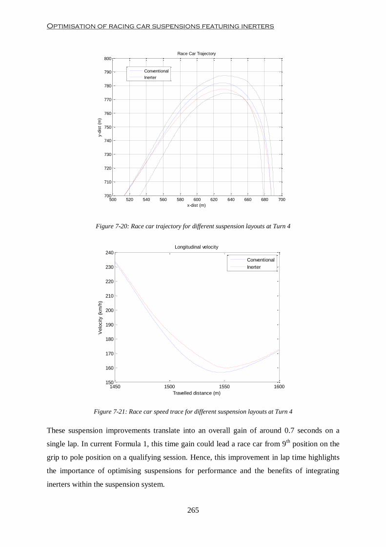
Optimisation of racing car suspensions featuring inerters
265
Figure 7-20: Race car trajectory for different suspension layouts at Turn 4
Figure 7-21: Race car speed trace for different suspension layouts at Turn 4
These suspension improvements translate into an overall gain of around 0.7 seconds on a
single lap. In current Formula 1, this time gain could lead a race car from 9th position on the
grip to pole position on a qualifying session. Hence, this improvement in lap time highlights
the importance of optimising suspensions for performance and the benefits of integrating
inerters within the suspension system.
500 520 540 560 580 600 620 640 660 680 700700
710
720
730
740
750
760
770
780
790
800Race Car Trajectory
x-dist (m)
y-d
ist
(m)
Conventional
Inerter
1450 1500 1550 1600150
160
170
180
190
200
210
220
230
240Longitudinal velocity
Travelled distance (m)
Velo
city (
km
/h)
Conventional
Inerter

Chapter 7- Suspension Performance Optimisation
266
7.7. Summary
In Chapter 7, the problem of suspension optimisation has been defined as a multi-objective
optimisation problem. Definition and discussion of both search (design variables) and
objective space (performance cost functions) have been carried out. A novel multi-stage
suspension optimisation methodology based on a virtual environment has been developed.
Finally, this method has been applied to obtain the optimal suspension setup of a race car for
two suspension layouts. This optimisation method has successfully provided suspension
solutions that maximises overall vehicle performance. Furthermore, results of the
optimisation process have shown that the use of inerters leads to significant improvements in
lap time (ultimate race car performance) with respect to conventional suspension layouts. The
main reason for this improvement is the enhanced aerodynamic platform and the improved
dynamic stability that can be achieved by the use of inerters.
It is also important to note that the main advantage of this optimisation methodology resides
in that fact that, even though external factors such as race track layout or aerodynamic
package will not affect the results obtained at the multi-objective stage, the selection of the
final solution will be conditioned by these factors. It is therefore expected that, under
different conditions such as a low-speed corner track layout and/or low downforce
configuration, the optimal suspension obtained from the optimisation process would have
been different from the one obtained in this case study. Hence, this methodology offers a
multi-level suspension optimisation procedure in which suspension dynamics are analysed in
isolation on a first level and then, complex interactions with the rest of vehicle systems are
integrated to evaluate the overall performance of race car.
This novel optimisation procedure also provides enhancements in the design and
development times of racing car suspension systems. Suspension solutions from the Pareto
front obtained as a result of the multi-objective optimisation stage can be used to create a
suspension setting database. Provided that no major changes are made in the fundamental
design of the suspension throughout a season, suspension designers could use this database as
baseline so that only final decision making process would be required in order to obtain the
optimal suspension setting for each particular event.
The next chapter summarises the achievements and original work in this research thesis, and
summarises some recommendations for future work.

Optimisation of racing car suspensions featuring inerters
267
8. Conclusions and Future Work
8.1. Summary of the Objectives Achieved
A formal method for optimising racing car suspension featuring inerters has been developed.
The key features of this method are the use of an experimentally validated model of a race car
suspension incorporating real mechanical inerters, the development of a robust and efficient
optimisation methodology based on multi-objective optimisation, surrogate modelling and
lap-time simulation and the definition of performance based suspension objective functions.
In Chapter 3, the dynamic behaviour of ideal inerters in a SDOF system has been
characterised. The conclusions of this theoretical analysis enhanced the current understanding
of the impact of the use of inerters on the dynamics of a vibratory system. The study also
drew some suggestions on how inerters could be used to improve the ride dynamics of a
vehicle suspension.
In Chapter 4, the design of a race car suspension fitted with real inerters has been carried out.
A ball-screw-type inerter was decided as design solution due to its design simplicity.
Moreover, the chassis frame and suspension system of a Formula Student car has been
modified and re-designed in order to accommodate all new suspension components including
the inerter devices. This vehicle has been used as test car in a 4-post rig test facility in order
to estimate vehicle parameters and to validate the vehicle suspension model developed in
Chapter 5. In order to properly acquire and estimate all the parameters of the test vehicle
incorporating real inerters, the parameter estimation software developed by Bennett (2012)
has been extended in order to account for the estimation of the vehicle suspension parameters
including real inerters and the definition of additional to dynamic frequency responses such
as front and rear ride height variation and dynamic longitudinal weight distribution variation.
In Chapter 5, a dynamic vehicle suspension model incorporating real inerters was developed.
This novel vehicle suspension model accounted for linearised suspension parasitic effects
such as suspension compliance, damper hysteresis and elastic and friction effects on the
inerter. Moreover, in order to accurately represent the tyre dynamic behaviour experienced
due to higher tyre deflections present with suspension systems incorporating inerters, a
nonlinear tyre model was developed in relation to the measured data obtained from 4-post rig
testing. Experimental data obtained from 4-post rig testing was used to evaluate the accuracy
Chapter 8- Conclusions and Fututre Work
268
of this model. A wide range of inerter settings were tested from light to heavy inertance
characteristics. Results showed that the vehicle suspension model incorporating real inerters
and a nonlinear vertical tyre model was capable of accurately replicating the dynamic
behaviour of the real vehicle for all the test cases proposed. Moreover, this vehicle
suspension model was used to perform a virtual optimisation in order to evaluate the
predicting capabilities of the model. The predicted suspension settings obtained from the
optimisation were used to set the suspension of the test car and experimental test was carried
out on the 4-post rig. Results showed that the vehicle suspension model successfully
predicted optimised suspension settings for two different performance objective functions.
In Chapter 6, a transient lap time simulation tool was developed. Based on work undertaken
by other authors (Casanova, 2000; Kelly, 2008), the problem of minimising lap-time around
a given track became one of calculating the minimum time for manoeuvring using Optimal
Control. Issues and limitations of classical techniques of the previous research works
(Casanova, 2000; Kelly, 2008) in the development of transient lap-time simulation tools were
addressed, and a novel solution technique based on a multi-level optimisation algorithm and
closed-loop driver steering has been developed. Furthermore, a full vehicle dynamic model
that incorporates the suspension model developed in Chapter 5 has been formulated. A case
study was carried out in order to evaluate the performance of this novel lap-time simulation
tool. A racing car model was forced to produce the fastest lap time around Bahrain
International GP Circuit. Results of the simulation demonstrated the efficiency and
robustness of the LTS solver.
Chapter 7 dealt with development of a novel suspension optimisation methodology. In order
to optimise the overall performance of a vehicle, suspension systems must successfully
achieve a number of goals simultaneously. Hence, due to the multi-criteria nature of
suspension design, the suspension optimisation problem was defined as a multi-objective
optimisation problem (MOOP). In this research work, suspension objective functions were
defined so that these functions express the impact of ride dynamics on the handling and
overall performance of the vehicle. Objective functions representing mechanical grip,
aerodynamic grip and understeer characteristic were developed. An NSGA-II evolutionary
algorithm was selected as the core search engine for optimisation, due to its suitability to
solve MOOPs. Computational efficiency and ability of finding the true optimal solution
issues were addressed. Solutions to these issues were proposed. Firstly, it was identified that
the numerical integration of the dynamic system every time the optimiser evaluates the

Optimisation of racing car suspensions featuring inerters
269
objective function caused the largest impact on the overall computational efficiency of the
optimisation process. A Kriging metamodelling technique has been used so that the
performance based objective functions are approximated to a more computationally efficient
mathematical model than the original dynamic model. A good correlation was found between
the results estimated by the metamodel and the actual results produced the original model.
The use of this surrogate model based optimisation technique successfully reduced the
computational time by over 90% of the optimisation time with the original vehicle model. A
Sequential Quadratic Programming (SQP) algorithm was coupled with the Multi-Objective
Evolutionary Algorithm (MOEA) to ensure that true optimal solutions were found. Two case
studies were analysed in the chapter: a conventional suspension and a new suspension
incorporating inerters. Results of this optimisation process showed that, due to conflicting
interactions among objective functions, the solution of the optimisation problem was
underdetermined, i.e. no single optimal solution was found. Instead of this, a trade-off of
optimised solutions were found (Pareto Optimal front). In order to find a single optimal
solution additional information was required. Hence, the lap-time simulation tool developed
in Chapter 6 was used to transform the underdetermined suspension optimisation problem
into a determined one. Solutions from the Pareto Optimal front obtained for both case studies
from previous stages of the optimisation process were introduced into the LTS. Results
showed that the suspension system incorporating inerters yielded important improvements in
the overall performance of the race car. It was demonstrated that the use of inerters
contributed to enhance the dynamic aerodynamic platform and to improve the overall
stability of the race car (less front-to-rear dynamic balance variations).
Results from the optimisation process show that the use of mechanical inerters in a racing car
suspension could theoretically produce performance gains of about 6 to 7 tenths of a second
over one lap. Although this might look like a very small gain in comparison to the overall lap
time (~ 85 secs), due to the competitive nature of the Motorsport industry, this gain could
mean a jump of between 7 and 10 positions on a qualifying session according to current F1
standards.
8.2. Recommendations for future work
This research work has developed a formal method for optimisation of race car suspensions
featuring inerters. The dynamic behaviour of inerters in mechanical systems has been
investigated and an experimentally validated suspension model has been developed. While

Chapter 8- Conclusions and Fututre Work
270
this thesis has yielded a few significant conclusions and contributions to the field of
suspension design and optimisation, further work would be highly desirable for improved
suspension performance with the use of passive elements. The recommendations for future
work are:
Enhancement of inerter technology: the dynamic analysis carried out in this research
thesis suggests that the use of complex inerters with nonlinear characteristics could
bring further improvements to suspension performance. Complex design solutions
could create an inerter that offers high inertance at low frequencies for optimal body
control and lower inertance at high frequencies for improved vibration at higher
frequencies. Moreover, a hydraulic inerter could be designed to create additional
damping effects as well as inertial effects, thereby improving the packaging and the
weight of the suspension.
Development of a nonlinear suspension model incorporating real inerters: in this
research work, the vehicle suspension was modelled as a transfer function G(s), that
accounts for linearised suspension component characteristics and linearised parasitic
effects. Although it showed good correlation with experimental data, it could not
replicate accurately enough highly nonlinear suspension properties such as bump stop
characteristics or highly nonlinear damper characteristics. Comprehensive modelling
of these characteristics would increase dramatically the complexity of the model and
this would reduce its computational efficiency. Alternatively, the suspension could be
modelled as a time-varying transfer function. In this way, the suspension is still
defined as an instantaneous linear model and suspension nonlinear parameters could
be passed as pre-calculated look-up tables.
Inclusion of suspension kinematics into the vehicle model: a validated vehicle
suspension model including kinematics could expand the range of analyses carried out
with the methodology developed in the thesis. The impact in vehicle performance of
kinematic variables such as tyre camber angle could be included as part of the
optimisation process. The kinematic suspension variables could be used to expand the
performance based objective functions in order to produce a complete optimisation of
a race car suspension.
Development of a more comprehensive nonlinear tyre model for ride analysis:
although the nonlinear semi-empirical tyre model developed in Chapter 5 showed
good correlation with experimental data, it cannot replicate nonlinear effects such as

Optimisation of racing car suspensions featuring inerters
271
hysteresis. A more comprehensive tyre model is expected to improve the correlation
with the vehicle model. Furthermore, tyre thermal and wear effects could be
introduced into this nonlinear tyre model. It is well known that tyre performance is
subjected mainly to wear condition and temperature and pressure changes. A model
that accounts for these effects could be used to develop a race simulator.
Application of inerter technology into production vehicles. Although the main focus
of this research work has been high performance racing applications, most of the work
developed could be directly applied to road cars. The development of advanced
passive suspensions featuring inerters could improve the comfort and safety
capabilities of production road cars without the expense of complex active suspension
systems.

272
References
Abdelhady, M. B. A., 2002. Aerodynamic Effects on Ride Comfort and Road Holding of
Actively Suspensed Vehicles. SAE Technical Paper 2002-01-2205.
Abdelhady, M. B. A. & Crolla, D. A., 1989. Theoretical Analysis of Active Suspension
Performance using a Four-Wheel Vehicle Model. Journal of Automobile Engineering,
Volume 203, pp. 125-135.
Akcay, H. & Turkay, S., 2009. Influence of tire damping on mixed H-2/H-infinity synthesis
of half-car active suspensions. Journal of Sound and Vibration, Volumen 322, pp. 15-28.
Al-Holou, N. et al., 2002. Sliding Mode Neural Network Inference Fuzzy Logic Control for
Active Suspension Systems. IEEE Transactions on Fuzzy Systems, 10(2), pp. 234-246.
Alkhatib, R., Jazar, G. N. & Golnaraghi, M. F., 2004. Optimal Design of Passive Linear
Suspension using Genetic Algorithm. Journal of Sound and Vibration, Volume 275, pp. 665-
691.
Allen, P. J., Hameed, A. & Goyder, H., 2006. Automotive damper model for use in multi-
body dynamic simulation. Journal of Automobile Engineering, Volume 220, pp. 1221-1233.
Allen, R. W. & Rosenthal, T. J., 1994. Requirements for Vehicle Dynamics Simulation
Models. SAE Technical Paper 940175.
Andersen, E. R., 2007. Multibody Dynamics Modeling and System Identification for a
Quarter-Car Test Rig with McPherson Strut Suspension, Virginia Polytechnic Institute:
Master Thesis.
Antoniou, A. & Lu, W.-S., 2007. Practical Optimization: Algorithms and Engineering
Applications. University of Victoria, Canada: Springer Science & Business Media, LLC.
Aschwanden, P., Müller, J. & Knörnschild, U., 2006. Experimental Study on the Influence of
Model Motion on the Aerodynamic Performance of a Race Car. SAE Technical Paper 2006-
01-0803.
Aschwanden, P., Müller, J., Travaglio, G. C. & Schöning, T., 2008. The Influence of Motion
Aerodynamics on the Simulation of Vehicle Dynamics. SAE Technical Paper 2008-01-0657.

273
Balike, K. P., 2010. Kineto-Dynamic Analysis Of Vehicle Suspension For Optimal Synthesis,
Concordia University: PhD thesis.
Barak, P., Panakanti, N. & Desai, T., 2004. Effect of Chassis Design Factors (CDF) on the
Ride Quality using a Seven Degree of Freedom Vehicle Model. SAE Technical Paper 2004-
01-1555.
Baumal, A., McPhee, J. & Calamai, P., 1998. Application of genetic algorithms to the design
optimization of an active vehicle suspension system. Computer Methods in Applied
Mechanics and Engineering, pp. 87-94.
Benedetti, A., Farina, M. & Gobbi, M., 2006. Evolutionary Multiobjective Industrial Design:
The Case of a Racing Car Tire-Suspension System. IEEE Transactions on Evolutionary
Computation, 10(3), pp. 230-244.
Bennett, L., 2012. Ride and Handling Assessment of Vehicles Using Four-post Rig Testing
and Simulation, Oxford Brookes University: PhD thesis.
Benson, D., 2005. A Gauss Pseudospectral transcription for Optimal Control, Massachusetts
Institute of Technology: PhD Thesis.
Betts, J. T., 2010. Practical Methods for Optimal Control and Estimation using Nonlinear
Programming. 2nd edition ed. Philadelphia: SIAM.
Biegler, L. T. & Zavala, V. M., 2008. Large-Scale Nonlinear Programming Using IPOPT: An
Integrating Framework for Enterprise-Wide Optimization. Computers and Chemical
Engineering, 33(3), p. 575–582.
Blank, M. & Margolis, D., 1996. The Effect of Normal Force Variation on the Lateral
Dynamics of Automobiles. SAE Technical Paper 960484.
Bleakney, W. M., Zielinski, L. F. & Ede, C. M., 1949. United States, Patent No. 2471857.
Boggs, C., Ahmadian, M. & Southward, S., 2008. Application of System Identification for
Efficient Suspension Tuning in High-Performance Vehicles: Quarter-Car Study. SAE
International Journal of Passenger Car - Mechanical Systems, 1(1), pp. 1298-1310.

274
Boggs, C., Ahmadian, M. & Southward, S., 2009. Application of System Identification for
Efficient Suspension Tuning in High-Performance Vehicles: Full-Car Model Study. SAE
International Journal of Passenger Cars - Mechanical Systems, pp. 622-635.
Bouazizi, M.-L., Ghanmi, S. & Bouhaddi, N., 2009. Multi-objective optimization in
dynamics of the structures with nonlinear behaviour: Contributions of the metamodels. Finite
Elements in Analysis and Design, 45(10), p. 612–623.
Braghin, F., Cheli, F., Melzi, S. & Sabbioni, E., 2008. Race Driver Model. Computer and
Structures, Volume 86, pp. 1503-1516.
Bramanti, A., Di Barba, P., Farina, M. & Savini, A., 2001. Combining respense surfaces and
evolutionary strategies for multiobjective pareto-optimization in electromagnetics.
International Journal of Applied Electromagnetics and Mechanics, Volume 15, pp. 231-236.
Brayshaw, D., 2004. The use of numerical optimisation to determine on-limit handling
behaviour of race cars, Cranfield University: PhD thesis.
Butz, T., Simeon, B. & Stadler, M., 2010. Optimal Design of Experiments for Estimating
Parameters of a Vehicle Dynamics Simulation Model. Journal of Computational and
Nonlinear Dynamics, 5(3), pp. 1011-1017.
Cambiaghi, D., Gadola, M. & D., V., 1998. Suspension System Testing and Tuning with the
Use of a Four-Post Rig. SAE Technical Paper 983023.
Cane Creek, 2012. Cane Creek Double Barrel Suspension. [Online]
Available at: http://www.canecreek.com/products/suspension/double-barrel
[Accessed 2010].
Cappelleri, D. J., Frecker, M. I., Simpson, T. W. & Snyder, A., 2002. Design of a PZT
Bimorph Actuator Using a Metamodel-Based Approach. Journal of Mechanical Design,
Volume 129, pp. 354-357.
Captain, K., Boghani, A. & Wormley, D., 1979. Analytical Tire Models for Dynamic Vehicle
Simulation. Vehicle System Dynamics, Volumen 8, pp. 1-32.
Casanova, D., 2000. On minimum time vehicle manouvrering: the theoretical optimal lap,
Cranfield University: PhD thesis.
275
Casanova, D., Sharp, R. S. & Symonds, P., 2000. Minimum Time Manoeuvring: The
Significance of Yaw Inertia. Vehicle System Dynamics, Volume 34, pp. 77-115.
Casanova, D., Sharp, R. S. & Symonds, P., 2001. Sensitivity to Mass Variations of the
Fastest Possible Lap of a Formula One Car. Vehicle System Dynamics, Volume 35, pp. 119-
134.
Casanova, D., Sharp, R. S. & Symonds, P., 2002. On the Optimisation of the Longitudinal
Location of the Mass Centre of a Formula One Car for two Circuits. Hiroshima, Japan, 6th
International Symposium on Advanced Vehicle Control.
Cheli, F., Dellachà, P. & Zorzutti, A., 2007. Optimization and Potentiality Study of a
Variable Kinematics Suspension. Las Vegas, USA, Proceedings of the ASME 2007
International Design Engineering Technical Conferences & Computers and Information in
Engineering Conference, pp. 1253-1260.
Chen, W., Garimella, R. & Michelena, N., 1999. Robust Design for Improved Vehicle
Handling under a Range of Maneuver Conditions. Las Vegas, USA, Proceedings of the 1999
ASME Design Engineering Technical Conferences.
Chi, Z., He, Y. & Naterer, G. F., 2008. Design Optimization of Vehicle Suspensions with a
Quarter-Vehicle Model. Transactions of the CSME, 32(2), pp. 297-312.
Chung, H.-S. & Alonso, J. J., 2004. Multiobjective optimization using approximation model-
based genetic algorithms. Albany, USA, 10th AIAA/ISSMO Symposium on
Multidisciplinary Analysis and Optimization.
Close, C. M. & K., F. D., 1995. Modeling and Analysis of Dynamic Systems. 2nd ed. New
York: John Wiley and Sons, Inc.
Cooke, R., Crolla, D. A. & Abe, M., 1997. Modelling Combined Ride and Handing
Manoeuvres for a Vehicle with slow-Active Suspension. Vehicle System Dynamics, Volume
27, pp. 457-476.
Dassault Systems Solidworks Corp., 2012. Solidworks. [Online]
Available at: http://www.solidworks.com/
Davis, B. R. & Thompson, A. G., 2001. Power Spectral Density of Road Profiles. Vehicle
System Dynamics, 35(6), pp. 409-415.

276
Deb, K., 2001. Multi-Objective Optimization using Evolutionary Algorithms. New York:
John Wiley & Sons, Ltd.
Deb, K. & Goel, T., 2001. A Hybrid Multi-Objective Evolutionary Approach to Engineering
Shape Design. Zurich, Switzerland, Proceedings of the First International Conference on
Evolutionary Multi-Criterion Optimization, pp. 385-399.
Deb, K., Pratap, A., Agarwal, S. & Meyarivan, T., 2002. A Fast and Elitist Multiobjective
Genetic Algorithm. IEEE Transactions on Evolutionary Computation, 6(2), pp. 182-197.
Del Castillo, J. M., Pintado, P. & Benitez, F. G., 1990. Optimization for Vehicle Suspension
II: Frequency Domain. Vehicle System Dynamics, Volume 19, pp. 331-352.
Deshpande, S., Mehta, S. & Jazar, G. N., 2006. Optimization of Secondary Suspension of
Piecewise Linear Vibration Isolation Systems. International Journal of Mechanical Sciences,
Volume 48, pp. 341-377.
Dominy, J. A. & Dominy, R. G., 1984. Aerodynamic Influences on the Performance of the
Grand Prix Racing Car. Journal of Automobile Engineering, 198(7), pp. 87-93.
Dominy, J. & Bullman, D. N., 1995. An Active Suspension for a Formula One Grand Prix
Racing Car. Journal of Dynamic Systems, Measurement, and Control, 107(1), pp. 73-79.
Dominy, R. G., 1992. Aerodynamics of Grand Prix Cars. Journal of Automobile Engineering,
Volume 206, pp. 267-274.
Els, P., Uys, P., Snyman, J. & Thoresson, M., 2006. Gradient-based approximation methods
applied to the optimal design of vehicle suspension systems using computational models with
severe inherent noise. Mathematical and Computer Modelling, Volume 43, p. 787–801.
Evangelou, S., Limebeer, D. J. N., Sharp, R. S. & Smith, M. C., 2007. Mechanical Steering
Compensators for High-Performance Motorcycles. Journal of Applied Mechanics, Volumen
74, pp. 332-346.
Fang, H., Rais-Rohani, M., Liu, Z. & Horstemeyer, M. F., 2005. A comparative study of
metamodeling methods for multiobjective crashwirthiness optimization. Computers and
Structures, Volume 83, pp. 2121-2136.

277
Floyd, S. & Law, E. H., 1994. Simulation and Analysis of Suspension and Aerodynamic
Interactions of Race Cars. SAE Technical Paper 942537.
Fonseca, C. M. & Fleming, P. J., 1995. An Overview of Evolutionary Algorithms in
Multiobjective Optimization. Evolutionary Computation, 3(1), pp. 1-16.
Forrester, A., Sobester, A. & Keane, A., 2008. Engineering Design Via Surrogate Modelling:
A practical guide. New York: John Wiley & Sons, Ltd.
Fricke, D. & Hogg, S., 2010. Implementation and Validation of Active Aerodynamic Force
Control During Race Vehicle 7-Post Testing. SAE International Journal of Materials and
Menufacturing, 3(1), pp. 550-558.
Fujioka, T. & Kimura, T., 1992. Numerical simulation of minimum-time cornering
behaviour. JSAE Review, 13(1), pp. 44-51.
Genta, G. & Morello, L., 2009. The Automotive Chassis. Berlin: Springer.
Georgiou, G. & Natsiavas, S., 2009. Optimal Selection of Suspension Parameters in Large
Scale Vehicle Models. Vehicle System Dynamics, 47(9), pp. 1147-1166.
Georgiou, G., Verros, G. & Natsiavas, S., 2007. Multi-Objective Optimization of Quarter-Car
Models with Passive or Semi-Active Suspension System. Vehicle System Dynamics, 45(1),
pp. 77-92.
Ghike, C. & Shim, T., 2008. Development of Integrated Chassis Control System for Vehicle
Handling Enhancement. Ann Arbor, USA, 2008 ASME Dynamic Systems and Control
Conference, pp. 1375-1382.
Gies, P. E. & Rumsey, R. D., 1962. United States, Patent No. 3018854.
Gillespie, T. D., 1992. Fundamentals of Vehicle Dynamics. Warrendale: SAE International.
Gill, P. E., Murray, W. & Saunders, M. A., 2002. SNOPT: An SQP Algorithm for Large-
Scale Constrained Optimization. SIAM Review, 47(1), p. 99–131.
Gobbi, M., Levi, F. & Mastinu, G., 2006. Multi-objective stochastic optimisation of the
suspension system of road vehicles. Journal of Sound and Vibration, Volume 298, pp. 1055-
1072.
278
Gobbi, M., Mastinu, G. & Doniselli, C., 1999. Optimising a Car Chassis. Vehicle System
Dynamics, Volumen 32, p. 149–170.
Goel, T. et al., 2007. Response surface approximation of Pareto optimal front in multi-
objective optimization. Computer Methods in Applied Mechanics and Engineering, Volume
196, pp. 879-893.
Graf, M. & Kosuch, S., 2008. Simulation with a Vertical Oscillationg Race Car Model. SAE
Technical Paper 2008-01-2963.
Hegazy, S. & Sandy, C., 2009. Vehicle Ride Comfort and Stability Performance Evaluation.
SAE Technical Paper 2009-01-2859.
Hendrikx, J. P. M., Meijlink, T. J. J. & Kriens, R. F. C., 1996. Application of optimal control
theory to inverse simulation of car handling. Vehicle System Dynamics, Volume 12, pp. 449-
462.
Hrovat, D., 1997. Survey of Advanced Suspension Developments and Related Optimal
Control Applications. Automatica, 33(10), pp. 1781-1817.
Huntington, G. T., 2007. Advancement and Analysis of a Gauss Pseudospectral
Transcription for Optimal Control Problems, Massachusetts Institute of Technology: PhD
thesis.
Jazar, G. N., Alkhatib, R. & Golnaraghi, M. F., 2006. Root Mean Square Optimization
Criterion for Vibration Behaviour of Linear Quarter Car using Analytical Methods. Vehicle
System Dynamics, 44(5), pp. 477-512.
Jin, R., Chen, W. & Simpson, T. W., 2000. Comparative Studies of Metamodeling
Techniques under Multiple Modeling Criteria. American Institute of Aeronautics and
Astronautics.
Jin, Y., 2005. A Comprehensive Survey of Fitness Approximation in Evolutionary
Computation. Journal of Soft Computing, 9(1), pp. 3-12.
Johnston, M., Rieveley, R., Johrendt, J. & Minaker, B., 2010. Metrics for Evaluating the Ride
Handling Compromise. SAE Technical Paper 2010-01-1139.
279
Kelly, D. P., 2008. Lap time simulation with transient vehicle and tyre dynamics, Cranfield
University: PhD thesis.
Kelly, J., Kowalczyk, H. & Oral, H. A., 2002. Track Simulation and Vehicle Characterization
with 7 Post Testing. SAE Technical Paper 2002-01-3307.
King, W. J., 1912. United States, Patent No. 1044188.
Kirk, D. E., 2004. Optimal Control Theory: An Introduction. Mineola: Dover Publications,
Inc.
Konak, A., Coit, D. W. & Smith, A. E., 2006. Multi-objective optimization using genetic
algorithms: A tutorial. Genetic Algorithms and Reliability, 91(9), pp. 992-1007.
Kowalczyk, H., 2002. Damper Tuning with the use of a Seven Post Shaker Rig. SAE
Technical Paper 2002-01-0804.
Kropác, O. & Múcka, P., 2008. Effect of obstacles in the road profile on the dynamic
response of a vehicle. Journal of Automobile Engineering, Volume 222, pp. 353-370.
Kuo, Y.-P., Pai, N.-S., Lin, J.-S. & Yang, C.-Y., 2008. Passive Vehicle Suspension System
Design Using Evolutionary Algorithm. Wuhan, China, IEEE International Symposium on
Knowledge Acquisition and Modeling Workshop, pp. 292 - 295.
Li, T.-H. S.-. & Kuo, Y.-P., 2000. Evolutionary Algorithms for Passive Suspension Systems.
International Journal of Mechanical Systems,Machine Elements and Manufacturing, 43(3),
pp. 537-544.
Loyer, B. & Jézéquel, L., 2009. Robust design of a passive linerar quarter car suspension
system using a multi-objective evolutionary algorithm and analytical robustness indexes.
Vehicle System Dynamics, 47(10), pp. 1253-1270.
Lu, J. & DePoyster, M., 2002. Multiobjective Optimal Suspension Control to Achieve
Integrated Ride and Handling Performance. IEEE Transactions on Control Systems
Technology, 10(6), pp. 807-821.
Lyu, N. et al., 2006. Design of automotive torsion beam suspension using lumped-compliance
linkage model. Chicago, USA, ASME 2006 International Mechanical Engineering Congress
and Exposition, pp. 219-228.
280
Maher, D., 2011. Combined Time and Frequency Domain Approaches to the Operational
Identification of Vehicle Suspension Systems, Dublin City University: PhD thesis.
Man, K. F., Tang, K. S. & Kwong, S., 1996. Genetic Algorithms: Concepts and Applications.
IEEE Transactions on Industrial Electronics, 43(5), pp. 519-534.
March, C. & Shim, T., 2007. Integrated control of suspension and front steering to enhance
vehicle handling. Journal of Automobile Engineering, Volume 221, pp. 377-391.
Mashadi, B. & Crolla, D. A., 2005. Influence of Ride Motions on the Handling Behaviour of
a Passenger Vehicle. Journal of Automobile Engineering, Volume 219, pp. 1047-1058.
MathWorks, 2010. Optimisation Toolbox User's Guide. Release 5.1 ed.
MathWorks, 2012. MathWorks - SimMechanics. [Online]
Available at: http://www.mathworks.co.uk/products/simmechanics/
MathWorks, 2012. MathWorks - Simulink. [Online]
Available at: http://www.mathworks.co.uk/products/simulink/
Metwalli, S. M., 1986. Optimum Nonlinear Suspension Systems. ASME Journal of
Mechanisms, Transmissions, and Automation in Design, 48(2), pp. 197-203.
Metz, D. & Williams, D., 1989. Near Time-Optimal Control of Racing Vehicles. Automatica,
25(6), pp. 841-857.
Miller, A., 2002. Testing a Formula SAE Racecar on a Seven-Poster Vehicle Dynamics
Simulator. SAE Technical Paper 2002-01-3309.
Milliken, W. F. & Milliken, D. L., 1995. Race Car Vehicle Dynamics. Warrendale: SAE
International.
Miura, Y., Tokutake, H. & Okubo, H., 2004. Cornering Time Estimation with Transient
Dynamics under Bump Disturbance. SAE Technical Paper 2004-01-3519.
Molina-Cristobal, A. y otros, 2007. Multi-Objective Controller Design: Evolutionary
Algorithms and Bilinear Matrix Inequalities for a Passive Suspension. International Journal
of Tmography and Stadistics, 7(F07), pp. 31-36.
281
MscSoftware, 2012. Msc Software - Adams. [Online]
Available at: http://www.mscsoftware.com/uk/Products/CAE-Tools/Adams.aspx
MÜhlmeier, M. & Müller, N., 2002. Optimization of the Driving Line on a Race Track. SAE
Technical Paper 2002-01-3339.
Multimatic Technical Centre, E., 2011. Multimatic Four Post Technical Specification and
Operating Manual, Thetford: Multimatic Technical Centre Europe.
Nocedal, J. & Wright, S. J., 2006. Numerical Optimization. 2 ed. Berlin: Springer Verlag.
Orlando, S., Peeters, B. & Coppotelli, G., 2008. Improved FRF estimators for MIMO Sine
Sweep data. Leuven, Belgium, Proceedings of ISMA 08 International Conference of Noise
and Vibration.
Pacjeka, H. B., 2006. Tire and Vehicle Dynamics. 2 ed. Oxford: BUTTERWORTH
HEINEMANN.
Papageorgiou, C., Lockwood, O. G., Houghton, N. E. & Smith, M. C., 2007. Experimental
testing and modelling of a passive mechanical steering compensator for high-performance
motorcycles. Kos, Greece, s.n., pp. 3592-3599.
Papageorgiou, C. & Smith, M., 2006. Positive Real Synthesis Using Matrix Inequalities for
Mechanical Networks: Application to Vehicle Suspension. IEEE Transactions on Control
Systems Technology, 14(3), pp. 423-435.
Papageorgiou, C. & Smith, M. C., 2005. Laboratory experimental testing of inerters. Seville,
Spain, Proceedings of the 44th IEEE Conference on Decision and Control.
Prokop, G., 2001. Modeling Human Vehicle Driving by Model Predictive Online
Optimization. Vehicle System Dynamics, 35(1), pp. 19-53.
Purdy, D. J. & Bullman, D. N., 1997. An experimental and theoretical investigation into the
design of an active suspension system for a racing car. Journal of Automobile Engineering,
211(3), pp. 161-173.
Queipo, N. V. et al., 2005. Surrogate based analysis and optimization. Journal of Progress in
Aerospace Sciences, Volume 41, pp. 1-28.
282
Rakheja, S. & Ahmed, A. K. W., 1991. simulation of Nonlinear Variable Dampers using
Energy Similary. Engineering Computations, Volume 8, pp. 333-344.
Sbalzarini, I. F., Müller, S. & Koumoutsakos, P., 2000. Multiobjective optimization using
Evolutionary Algorithms. Stanford, USA, s.n., pp. 63-74.
Scheibe, F. & Smith, M. C., 2009. Analytical solutions for optimal ride comfort and tyre grip
for passive vehicle suspensions. Vehicle System Dynamics, 47(10), pp. 1229-1252.
Schmitt, K., Madsen, J., Anitescu, M. & Negrut, D., 2008. A Gaussian Process Based
Approach for Handling uncertainity in Vehicle Dynamics Simulation. Boston, USA, ASME
2008 International Mechanical Engineering Congress and Exposition, pp. 617-628.
Seqveland, I. E., 1933. United States, Patent No. 1933768.
Shannan, J. E. & Vanderploeg, M. J., 1989. A Vehicle Handling Model with Active
Suspensions. Journal of Mechanisms, Transmissions and Automation in Design, Volume
111, pp. 375-380.
Sharp, R. S., Hassan & A., S., 1987. The Relative Performance Capabilities of Passive,
Active and Semi-Active Car Suspension Systems. Journal of Automobile Engineering,
200(3), pp. 219-228.
Shihani, N., Kumbhar, B. K. & Kulshreshtha, M., 2006. Modeling of Extrusion Process using
Response Surface Methodology and Artificial Neural Networks. Journal of Engineering
Science and Technology, 1(1), pp. 31-40.
Shim, T. & Ghike, C., 2007. Understanding the limitations of different vehicle models for roll
dynamics studies. Vehicle System Dynamics, 45(3), pp. 191-216.
Shim, T. & Margolis, D., 2005. Dynamic Normal Force Control for Vehicle Stability
Enhancement. International Journal of Vehicle Autonomous Systems, 3(1), pp. 1-14.
Shirahatt, A., Prasad, P., Panzade, P. & Kulkarni, M., 2008. Optimal design of passenger car
suspension for ride and road holding. Journal of the Brazilian Society of Mechanical Sciences
and Engineering, 30(1), pp. 66-76.
283
Siegler, B., Deakin, A. & Crolla, D. A., 2000. Lap Time Simulation: Comparison of Steady
State, Quasi- Static and Transient Racing Car Cornering Strategies. SAE Technical Paper
2000-01-3563.
Simpson, T. W., 1998. Comparison of Response Surface and Kriging Models in the
Multidisciplinary Design of an Aerospike Nozzle. Institute for Computer Applications in
Science and Engineering (ICASE) Report 98-16.
Simpson, T. W., Korte, J. J., Mauery, T. M. & Mistree, F., 2001. Kriging Models for Global
Approximation in Simulation-Based Multidisciplinary Design Optimization. American
Institute of Aeronautics and Astronautics, 39(12), pp. 2233-2241.
Simpson, T. W., Peplinski, J., Koch, P. N. & Allen, J. K., 2001. Metamodels for computer-
based engineering design: survey and recommendations. Engineering with Computers,
Volume 17, pp. 129-150.
Smith, M. C., 2002. Synthesis of Mechanical Networks: The Inerter. IEEE Transactions on
Automatic Control, 46(10), pp. 1648-1662.
Smith, M. C., 2003. The Inerter Concept and Its Application. Fukui, Japan, Society of
Instrument and Control Engineers (SICE) Annual Conference.
Smith, M. C., 2006. Passive Network Synthesis Revisited. Kyoto, Japan, 17th International
Symposium on Mathematical Theory of Networks and Systems.
Smith, M. C. & Wang, F.-C., 2004. Performance Benefits in Passive Vehicle Suspension
employing Inerters. Vehicle System Dynamics, pp. 235-257.
Soliman, A. M. A., Abd Allah, S. A., El-Beter, A. A. & Hamid, M. S., 2001. Effect of
Suspension Spring Stiffness on Vehicle Dynamics. International Journal of Vehicle Design,
8(3/4), pp. 316-334.
Soliman, A. M. A., Moustafa, S. M. & Shogae, A. O. M., 2008. Parameters Affecting Vehicle
Ride Comfort using Half Vehicle Model. SAE Technical Paper 2008-01-1146.
Southward, S. C. & Boggs, M. B., 2008. Comparison of the Performance of 7-Post and 8-
Post Dynamic Shaker Rigs for Vehicle Dynamics Studies. SAE Technical Paper 2008-01-
2966.

284
Stamatov, S., Krishnan, M. & Yost, S. A., 2007. Using Quasi-linearization for Real Time
Dynamic Simulation of a Quarter Vehicle Suspension. SAE Technical Paper 2007-01-0833.
Stone, M. R. & Demetriou, M. A., 2000. Modeling and Simulation of Vehicle Ride and
Handling Performance. Rio, Greece, Proceedings of the 15th lEEE lntemational Symposium
on Intelligent Control, pp. 85-89.
Storey, I., Bourmistrova, A. & Subic, A., 2006. Multiobjective Optimisation of Control of
Active and Semi-Active Suspension Systems using Jerk as a measure of Comfort. Yokohama,
Japan, Fisita 2006.
Sun, P.-Y. & Chen, H., 2003. Multiobjective output-feedback suspension control on a half-
car model. Istanbul, Turkey, Proceedings of 2003 IEEE Conference on Control Applications,
pp. 290-295.
Sun, T., Zhang, Y. & Barak, P., 2002. 4-DOF Vehicle Ride Model. SAE Technical Paper
2002-01-1580.
Sun, W. et al., 2010. Ride-comfort-oriented suspension optimization using the pseudo-
excitation method. Journal of Automobile Engineering, Volume 224, pp. 1357-1367.
Tauscher, H., 1928. United States, Patent No. 1654763.
THK Co., Ltd., 2012. THK - Precision Ball Screw Product Descriptions. [Online]
Available at: https://tech.thk.com/en/products/thk_cat_main.php?id=359
[Accessed 2010].
THK Co., Ltd., 2012. THK Global. [Online]
Available at: http://www.thk.com/
Thompson, A. G., 1973. Quadratic Performance Indices and Optimum Suspension Design.
Proceedings of the Institution of Mechanical Engineers, 187(1), pp. 129-139.
Thompson, A. G., 1983. Suspension Design for Optimum Road-Holding. SAE Technical
Paper 830663.
Thoresson, M., Uys, P., Els, P. & Snyman, J., 2009. Efficient optimisation of a vehicle
suspension system, using a gradient-based approximation method, Part 1: Mathematical
modelling. Mathematical and Computer Modelling, Volume 50, pp. 1421-1436.
285
Thoresson, M., Uys, P., Els, P. & Snyman, J., 2009. Efficient optimisation of a vehicle
suspension system, using a gradient-based approximation method, Part 2: Optimisation
results. Mathematical and Computer Modelling, Volume 50, pp. 1437-1447.
Timings, J. & Cole, D., 2011. Efficient minimum manoeuvre time optimisation of an
oversteering vehicle at constant forward speed. San Francisco, USA, American Control
Conference (ACC), pp. 5267 - 5272.
Timings, J. P. & Cole, D. J., 2010. Minimum manoeuvre time of a nonlinear vehicle at
constant forward speed using convex optimisation. Loughborough, UK, Proceedings of the
10th International Symposium on Advanced Vehicle Control.
Todd, K. B. & Kulakowski, B. T., 1990. Handling Performance of Road Vehicles with
different Active Suspensions. Dallas, USA, Winter Annual Meeting of the American Society
of Mechanical Engineers, pp. 19-26.
Ullman, D. G., 1997. The Mechanical Design Process. New York: McGraw-Hill.
Vaidyanathan, R., Tucker, P. K., Papila, N. & Shyy, W., 2004. Computational-fluid-
dynamics-based design optimization for single-element rocket injector. Journal of Prpulsion
and Power, 20(4), pp. 705-717.
Velenis, E. & Tsiotras, P., 2005. Minimum Time vs. Maximum Exit Velocity Path
Optimization During Cornering. Dubrovnik, Croatia, Proceedings of the IEEE International
Symposium on Industrial Electronics, pp. 355 - 360.
Velenis, E. & Tsiotras, P., 2005. Optimal velocity profile generation for given acceleration
limits: receding horizon implementation. Atlanta, USA, Proceedings of the 2005 American
Control Conference, pp. 2147 - 2152.
Velenis, E. & Tsiotras, P., 2005. Optimal velocity profile generation for given acceleration
limits: theoretical analysis. Atlanta, USA, Proceedings of the 2005 American Control
Conference, pp. 1478 - 1483.
Venkatamaran, P., 2002. Applied Optimization with MATLAB programming. New York: John
Wiley & Sons, Inc.
286
Verros, G., Natsiavas, S. & Papadimitriou, C., 2005. Design Optimization of Quarter-car
Models with Passive and Semi-active Suspensions under Random Road Excitation. Journal
of Vibration and Control, Volumen 11, p. 581–606.
Wang, F.-. C., Chen, C.-. W., Liao, M.-. K. & Hong, M.-. F., 2007. Performance Analyses of
Building Suspension Control with Inerters. New Orleand, USA, Proceedings of the 46th
IEEE Conference on Decision and Control, pp. 3786-3791.
Wang, F.-C. & Chan, H.-A., 2008. Mechatronic Suspension Design and Its Applications to
Vehicle Suspension Control. Cancun, Mexico, Proceedings of the 47th IEEE Conference on
Decision and Control, pp. 3769-3774.
Wang, F.-. C., Hong, M.-. F. & Chen, C.-. W., 2010. Building suspensions with inerters.
Journal of Mechanical Engineering Science, 224(8), pp. 1605-1616.
Wang, F.-. C. & Su, W.-J., 2008. Inerter Nonlinearities and the Impact on Suspension
Control. Seattle, USA, American Control Conference, pp. 3245-3250.
Wang, F.-C., Hong, M.-F. & Lin, T.-C., 2011. Designing and testing a hydraulic inerter.
Journal of Mechanical Engineering Science, 225(1), pp. 66-72.
Wang, F.-C., Hsu, M.-S., Su, W.-J. & Lin, T.-C., 2009. s.l. Patent No. US 2009/0108510.
Wang, F.-C., Yu, C.-H., Chang, M.-L. & Hsu, M., 2006. The performance Improvements of
Train Suspension Systems with Inerters. San Diego, USA, Proceedings of the 45th IEEE
Conference on Decision and Control, pp. 1472-1477.
Wang, G. G. & Shan, S., 2007. Review of Metamodelling Techniques in Support of
Engineering Design Optimisation. Journal of Mechanical design, 129(4), pp. 370-380.
Wang, J., Wilson, D. A., Xu, W. & Crolla, D. A., 2006. Integrated Vehicle Ride and Steady-
State Handling Control via Active Suspensions. International Journal of Vehicle Design,
42(3/4), pp. 306-326.
Watres, L. S., 1908. United States, Patent No. 893680.
Weise, T., 2011. Global Optimization Algorithms: Theory and Application. 3 ed. E-book:
http://www.it-weise.de/.

287
Wentao, X., Tongchen, M. & Zheng, L., 2011. An Efficient Multi-objective Optimization
Method for Complicated Vehicle Random Vibration. Applied Mechanics and Materials,
Volume 94-96, pp. 1694-1700.
Whitehead, R., Travis, W., Bevly, D. M. & Flowers, G., 2004. A Study of the Effect of
Various Vehicle Properties on Rollover Propensity. SAE Technical Paper 2004-01-2094.
Williams, D. E. & Haddad, W. M., 1997. Active Suspension Control to improve Vehicle Ride
and Handling. Vehicle System Dynamics, Volumen 28, pp. 1-24.
Williams, R. A., 1997. Automotive Active Suspensions. Part 1: Basic Principles. Journal of
Automobile Engineering, Volumen 211, pp. 415-426.
Wilson, B., Cappelleri, D., Simpson, T. W. & Frecker, M., 2001. Efficient Pareto Frontier
Exploration using Surrogate Approximations. Optimization and Engineering, Volume 2, p.
31–50.
Wright, P. G., 1982. The Influence of Aerodynamics on the Design of Formula One Racing
Cars. International Journal of Vehicle Design, 3(4), pp. 383-397.
Yang, R. S. & Huang, X. D., 2009. Multi-Objective Optimization of Vehicle Handling and
Ride Comfort by Approximation Model. Manchester, UK, Proceedings of 2nd International
Conference on Modelling and Simulation, pp. 242-246.
Yildirim, S. & Eski, I., 2009. Vibration Analysis of an Experimental Suspension System
using Artificial Neural Networks. SAE Technical Paper 2009-01-0734.
Ziegenmeyer, J. D., 2007. Estimation of Disturbance Inputs to a Tire Coupled Quarter-car
Suspension Test Rig, Virginia Polytechnic Institute: Master thesis.
Zitzler, E., Thiele, L. & Deb, K., 2000. Comparison of Multiobjective Evolutionary
Algorithms: Empirical Results. Evolutionary Computation, Volume 8, pp. 173-195.

288
Appendix A: OBU Four-post rig Calibration Certificate
295
Appendix B: Derivation of Vehicle Equations of Motion
Appendix B derives the equations of motion of the vehicle model used in Chapter 6 for its
use into lap-time simulation. Figure B- 1 and Figure B- 2 show a schematic diagram of the
vehicle model in plan and lateral views.
Figure B- 1: Schematic plan view of vehicle model for lap-time simulation
Figure B- 2: Schematic lateral view of vehicle model for lap-time simulation
XG
ZG
zr
zuF
zs, w
φv
zL
xL
ωuR ωuF
zuR
q
xLU
zLU
a b
wb
XG
YG
ψv
yLS
xLS
δ
(xv,yv)
u
v
r
xLU
yLU

296
Definition of DOFs of the vehicle model and reference frame
First, considering the vehicle model shown in Figure B- 1 and Figure B- 2, three reference
frames have been defined: firstly, a global inertial frame XGYGZG (black coloured reference
frame), a non-inertial sprung mass fixed reference frame xSySzS (red coloured reference
frame) and a local frame moving with the CoG of the unsprung mass of the vehicle xUyUzU
(green coloured reference frame).
As introduced in Chapter 6, a lumped parameter single-track vehicle model has been used in
this thesis to evaluate the impact of ride dynamics on the performance of the race car. The
model consists of three bodies: one solid-rigid body that represents sprung mass ms and two
more bodies that represent front and rear wheels muf and mur respectively. This model
presents 9 DOFs. The model allows translational motion of the vehicle in all three
dimensions in space (longitudinal, lateral and vertical motions) and rotations around two axes
(yaw and pitch motion). Front and rear unsprung wheels are connected to the main body via a
suspension system. Unsprung masses are assumed to have motion only in vertical direction.
Moreover, wheels are allowed to rotate only about the spin axis. According to this, the vector
of generalised displacement (linear and angular) coordinates q that includes these motions
can be defined as:
Moreover, for vehicle modelling is more appropriate to express these motions in terms of
velocities rather than displacements. Therefore, a vector of velocities w related to generalised
displacements q can be defined as:
Where for j=F,R
Note that, the velocities expressed in vector w are related to non-inertial reference frames. In
order to express these variables with respect to an inertial reference frame, rotation matrices
between references frames must be defined. According to this, the sprung mass reference
frame xSySzS moves and rotates with the CoG of the sprung mass. Since the vehicle model
presents rotations in two axis (yaw and pitch motions), two rotation matrices R1 (yaw
rotation) and R2 (pitch rotation) can be defined:

297
These two rotations can be then combined so that translational motions in a local reference
frame can be expressed in a global inertial reference frame. A general transformation matrix
for translational motion Rtrans can be obtained by multiplying matrices (B.3) and (B.4):
In addition to this, a rotation matrix for rotational motions Rrot can be also defined as:
Since, the unsprung mass reference frame xUyUzU does not rotate with respect to respect to the
global inertial reference frame XGYGZG, the transformation matrix for unsprung mass motions
Ru can be expressed as an identity matrix:
Transformation of Lagrange Energy Method for quasi-velocities
The general Lagrange Energy Method must be re-arranged into a Lagrange Energy Method
for quasi-velocities when velocities related to non-inertial reference frames are used as
generalised coordinates (Genta & Morello, 2009). Therefore, the modified expression for the
Lagrange method can be defined as follows:
Where represents the Lagrangian of the system
T represents the total kinetic energy of the system
U represents the total potential energy of the system

298
D represents the total energy dissipation term
represents the vector of n quasi-velocities expressed with respect to a moving
frame reference frame
represents the vector of n generalised coordinates expressed with respect to a
global frame reference frame
represents the vector of generalised forces
B represents the rotation matrix from quasi-velocities to generalised velocities so that
[ ]
represents the gamma operator with
In this thesis, all forces generated from engine/brake, suspension, aerodynamic and tyre
systems have been considered as external generalised forces Qi.
The total kinetic energy of the system T can be obtained as follows:
Where : Total kinetic energy carried by the sprung mass
: Kinetic energy due to translational motion of the sprung mass
: Kinetic energy due to rotational motion of the sprung mass
: Translational velocity vector of the sprung mass
: Rotational velocity vector of the sprung mass
: Inertia tensor of sprung mass
: Total kinetic energy carried by the unsprung mass j
: Kinetic energy due to translational motion of the unsprung mass j
299
: Kinetic energy due to rotational motion of the unsprung mass
: Translational velocity vector of the front sprung mass
: Translational velocity vector of the rear sprung mass
: Rotational velocity vector of the unsprung mass j
: Inertia tensor of unsprung mass j
For j=F, R
Accordingly, the total potential energy of the system U can be calculated as:
Where : Potential energy of the sprung mass
: Potential energy of the unsprung mass j
Moreover, the rotation matrix A can be composed of rotation matrices (B.5) to (B.7) as
follows:
In this thesis, D=0 because all forces generated from suspension and tyre systems have been
considered as external generalised forces Qi.
Derivation of EOMs
Assuming small angle approximation, the EOMs describing the dynamic behaviour of the
vehicle can be derived from the Lagrange Method for quasi-velocities (see equation (B.9)):
300
Moreover, the generalised forces Q can be obtained as follows:
State-Space Model Representation
Recalling the definition of a dynamic system in state-space representation:
Where x(t) represents the vector of states of the system
u(t) represents the vector of inputs
t represents the independent variable time
According to this, the vector of states x(t) can be defined as a combination of vectors w and
q:
Equations (B.12) and (B.13) can then be combined and re-arranged to produce the final state-
space representation:
301