Prepared by Volkan OBAN

ggplot2 Examples:

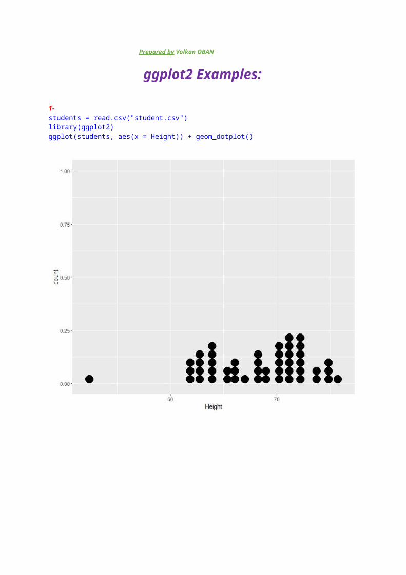
1-students = read.csv("student.csv")library(ggplot2)ggplot(students, aes(x = Height)) + geom_dotplot()

2-

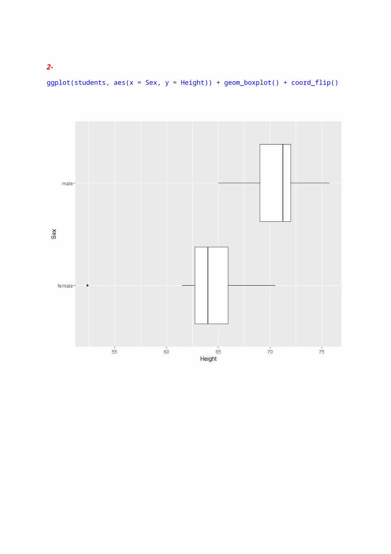
ggplot(students, aes(x = Sex, y = Height)) + geom_boxplot() + coord_flip()

3-

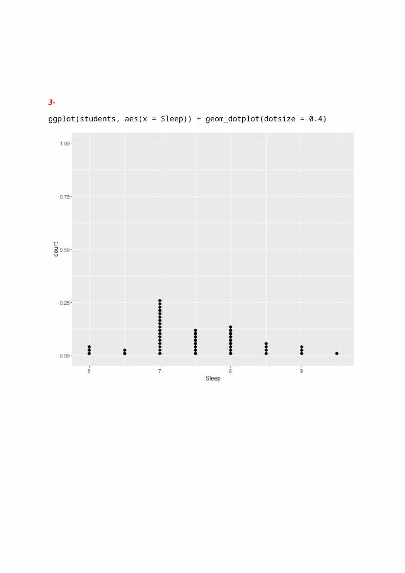
ggplot(students, aes(x = Sleep)) + geom_dotplot(dotsize = 0.4)

4-

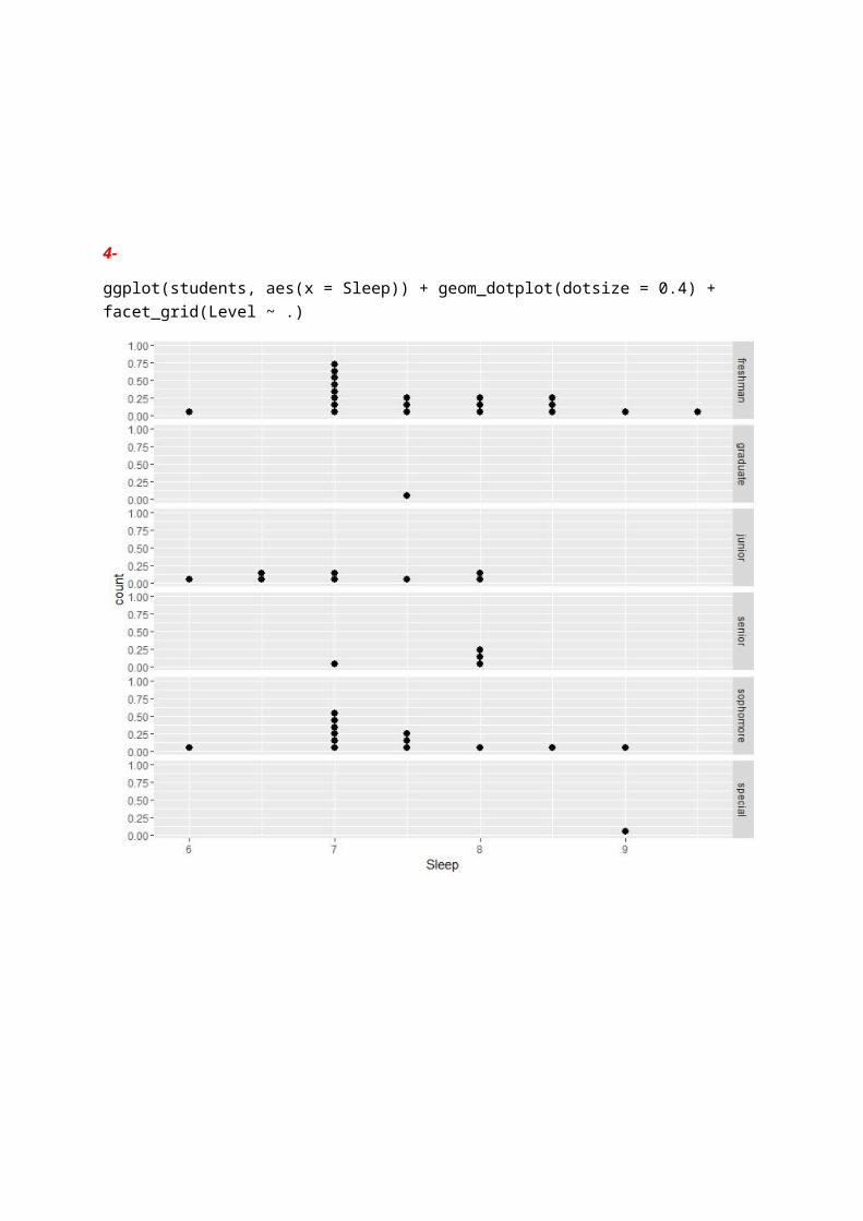
ggplot(students, aes(x = Sleep)) + geom_dotplot(dotsize = 0.4) + facet_grid(Level ~ .)

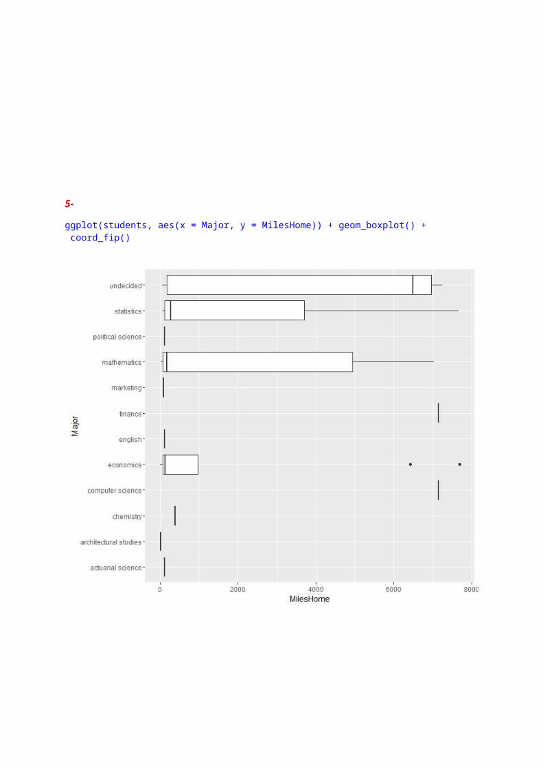
5-

ggplot(students, aes(x = Major, y = MilesHome)) + geom_boxplot() + coord_fip()

qplot

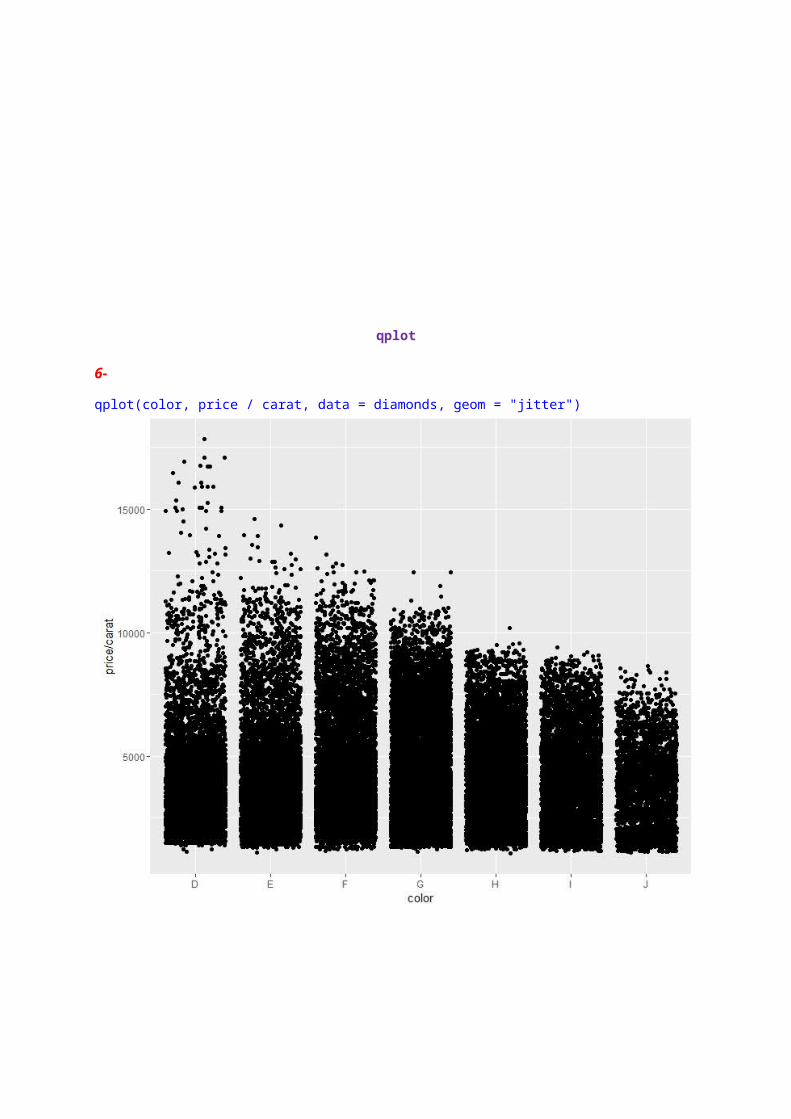
6-

qplot(color, price / carat, data = diamonds, geom = "jitter")

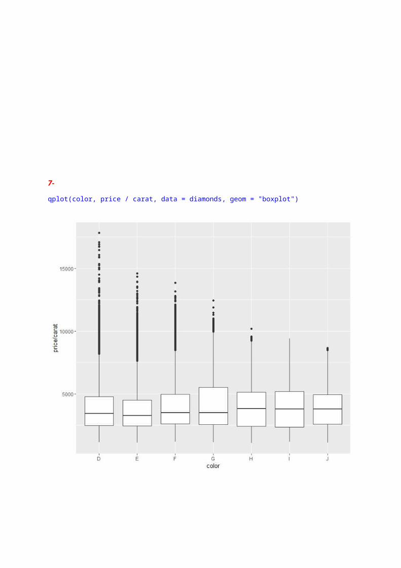
7-

qplot(color, price / carat, data = diamonds, geom = "boxplot")

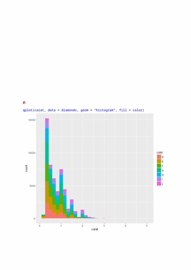
8-

qplot(carat, data = diamonds, geom = "histogram", fill = color)

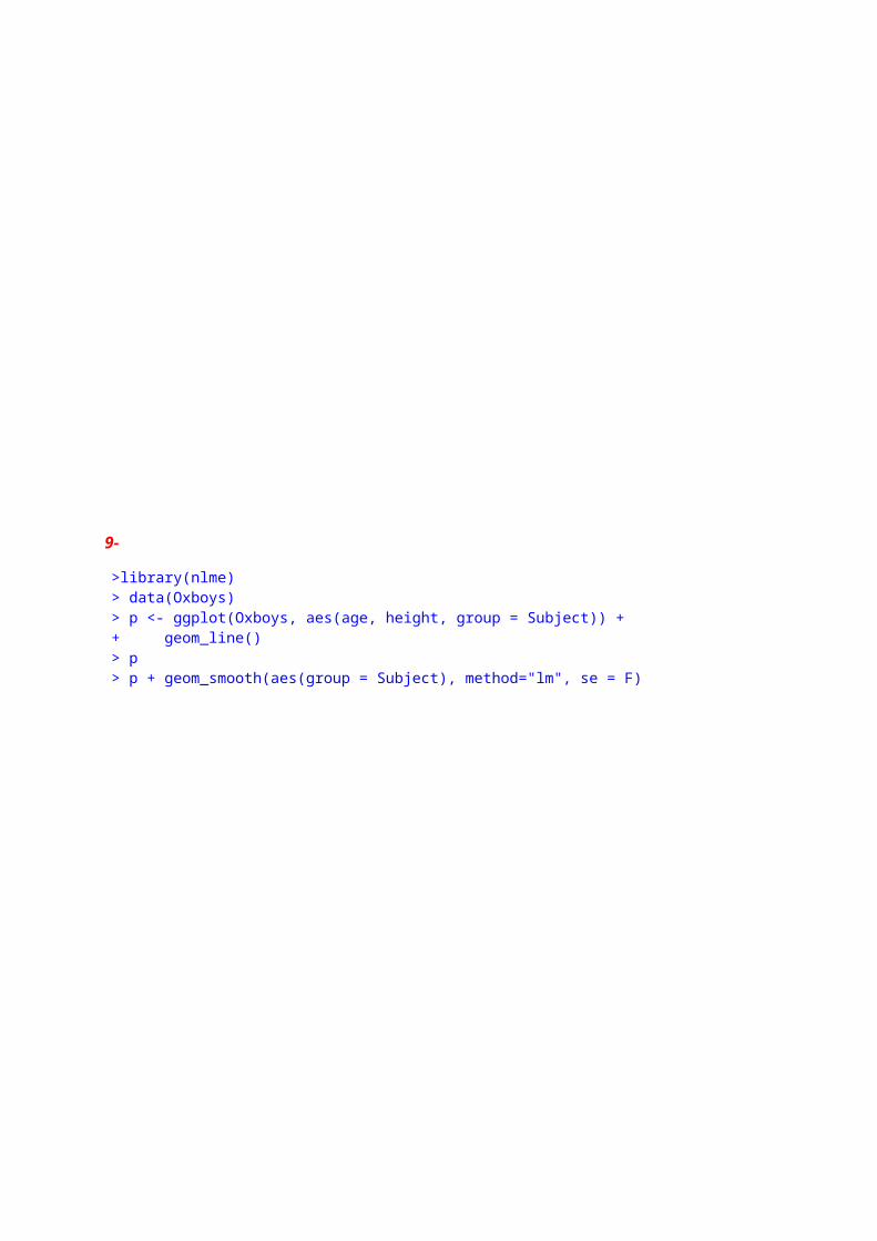
9-

>library(nlme)> data(Oxboys)> p <- ggplot(Oxboys, aes(age, height, group = Subject)) ++ geom_line()> p> p + geom_smooth(aes(group = Subject), method="lm", se = F)

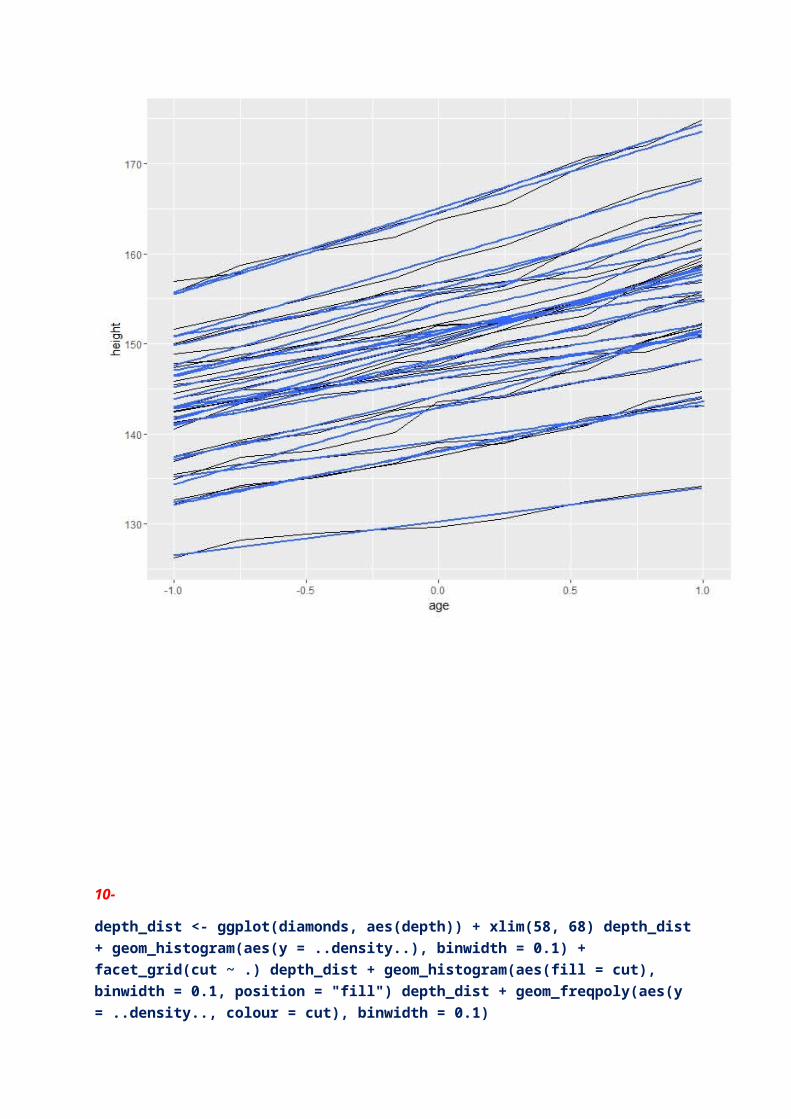
10-

depth_dist <- ggplot(diamonds, aes(depth)) + xlim(58, 68) depth_dist + geom_histogram(aes(y = ..density..), binwidth = 0.1) + facet_grid(cut ~ .) depth_dist + geom_histogram(aes(fill = cut), binwidth = 0.1, position = "fill") depth_dist + geom_freqpoly(aes(y = ..density.., colour = cut), binwidth = 0.1)

Reference: http://www.stat.wisc.edu/~larget/stat302/chap2.pdf

Reference book : ggplot2 Elegant Graphics for Data Analysis; Wickham, Hadley

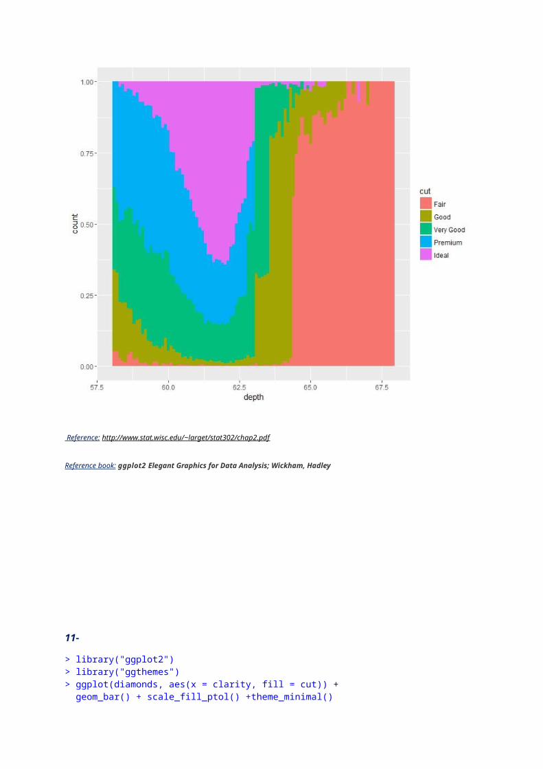
11-

> library("ggplot2")> library("ggthemes")> ggplot(diamonds, aes(x = clarity, fill = cut)) + geom_bar() + scale_fill_ptol() +theme_minimal()

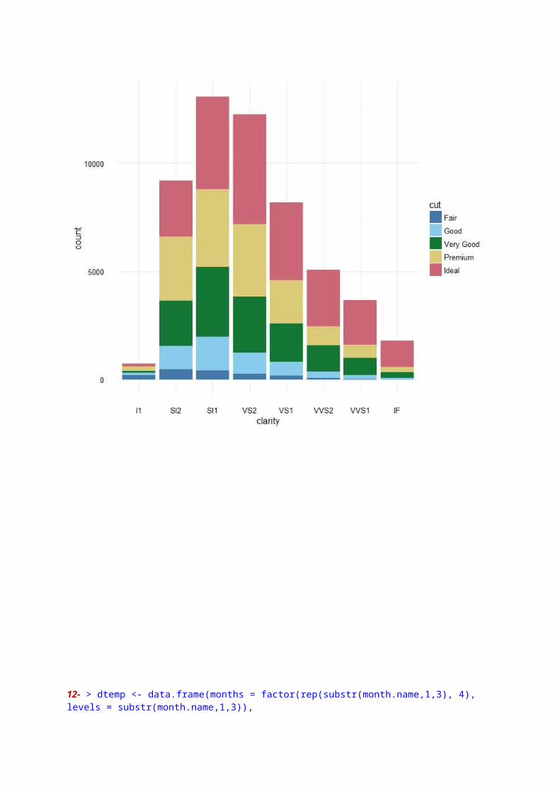
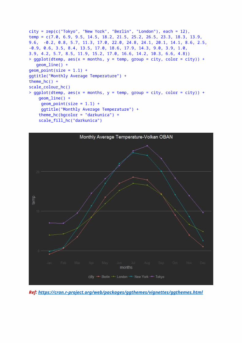
12- > dtemp <- data.frame(months = factor(rep(substr(month.name,1,3), 4), levels = substr(month.name,1,3)),city = rep(c("Tokyo", "New York", "Berlin", "London"), each = 12),temp = c(7.0, 6.9, 9.5, 14.5, 18.2, 21.5, 25.2, 26.5, 23.3, 18.3, 13.9, 9.6, -0.2, 0.8, 5.7, 11.3, 17.0, 22.0, 24.8, 24.1, 20.1, 14.1, 8.6, 2.5,-0.9, 0.6, 3.5, 8.4, 13.5, 17.0, 18.6, 17.9, 14.3, 9.0, 3.9, 1.0,3.9, 4.2, 5.7, 8.5, 11.9, 15.2, 17.0, 16.6, 14.2, 10.3, 6.6, 4.8))> ggplot(dtemp, aes(x = months, y = temp, group = city, color = city)) + geom_line() +geom_point(size = 1.1) + ggtitle("Monthly Average Temperature") +theme_hc() +scale_colour_hc()> ggplot(dtemp, aes(x = months, y = temp, group = city, color = city)) + geom_line() + geom_point(size = 1.1) + ggtitle("Monthly Average Temperature") + theme_hc(bgcolor = "darkunica") + scale_fill_hc("darkunica")

Ref: https://cran.r-project.org/web/packages/ggthemes/vignettes/ggthemes.html

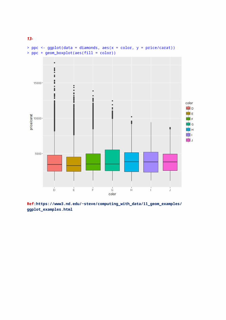
13-

> ppc <- ggplot(data = diamonds, aes(x = color, y = price/carat))> ppc + geom_boxplot(aes(fill = color))

Ref:https://www3.nd.edu/~steve/computing_with_data/11_geom_examples/ggplot_examples.html

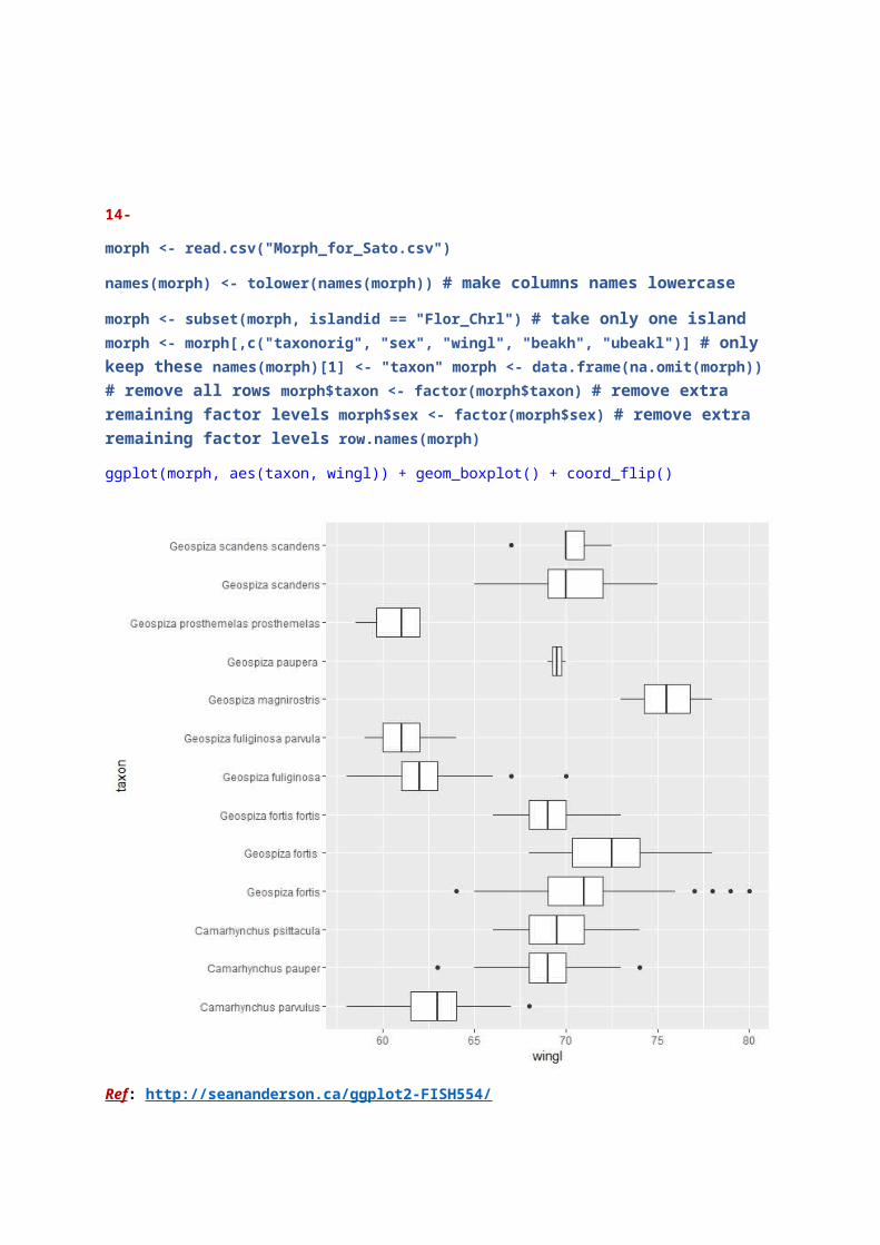
14-

morph <- read.csv("Morph_for_Sato.csv")

names(morph) <- tolower(names(morph)) # make columns names lowercase

morph <- subset(morph, islandid == "Flor_Chrl") # take only one island morph <- morph[,c("taxonorig", "sex", "wingl", "beakh", "ubeakl")] # only keep these names(morph)[1] <- "taxon" morph <- data.frame(na.omit(morph)) # remove all rows morph$taxon <- factor(morph$taxon) # remove extra remaining factor levels morph$sex <- factor(morph$sex) # remove extra remaining factor levels row.names(morph)

ggplot(morph, aes(taxon, wingl)) + geom_boxplot() + coord_flip()

Ref: http://seananderson.ca/ggplot2-FISH554/

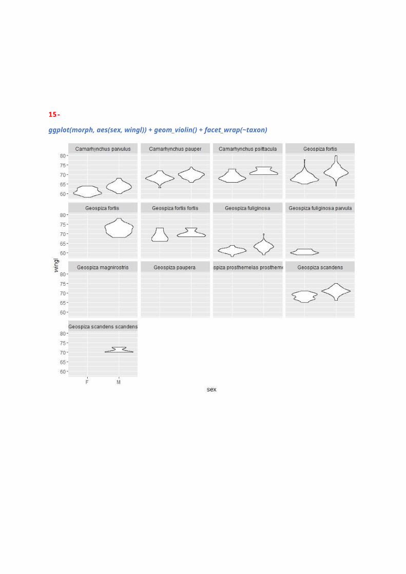
15-

ggplot(morph, aes(sex, wingl)) + geom_violin() + facet_wrap(~taxon)

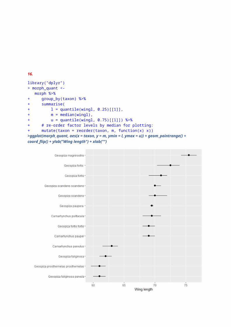
16.

library("dplyr")> morph_quant <- morph %>%+ group_by(taxon) %>%+ summarise(+ l = quantile(wingl, 0.25)[[1]],+ m = median(wingl),+ u = quantile(wingl, 0.75)[[1]]) %>%+ # re-order factor levels by median for plotting:+ mutate(taxon = reorder(taxon, m, function(x) x)) >ggplot(morph_quant, aes(x = taxon, y = m, ymin = l, ymax = u)) + geom_pointrange() + coord_flip() + ylab("Wing length") + xlab("")

Ref: http://seananderson.ca/ggplot2-FISH554/

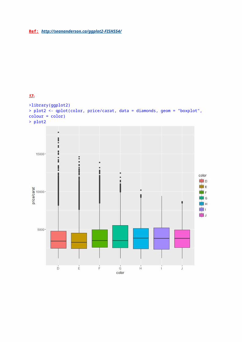
17-

>library(ggplot2)> plot2 <- qplot(color, price/carat, data = diamonds, geom = "boxplot", colour = color) > plot2

18-

> library(GGally)

> library(ggplot2)

>data(tips, package = "reshape")

> pm <- ggpairs(tips, mapping = aes(color = sex), columns = c("total_bill", "time", "tip"))

> pm

Ref: http://ggobi.github.io/ggally/docs.html#columns_and_mapping