Quick-Sort 1

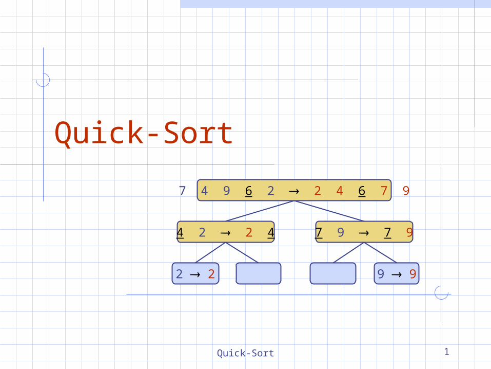
Quick-Sort

7 4 9 6 2 2 4 6 7 9

4 2 2 4 7 9 7 9

2 2 9 9

Quick-Sort 2

Outline and Reading

Quick-sort (§10.3) Algorithm Partition step Quick-sort tree Execution example

Analysis of quick-sort (§10.3.1)In-place quick-sort (§10.3.1)Summary of sorting algorithms

Quick-Sort 3

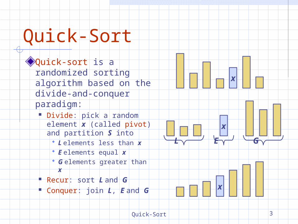
Quick-SortQuick-sort is a randomized sorting algorithm based on the divide-and-conquer paradigm:

Divide: pick a random element x (called pivot) and partition S into

L elements less than x E elements equal x G elements greater than

x Recur: sort L and G Conquer: join L, E and G

x

x

L GE

x

Quick-Sort 4

PartitionWe partition an input sequence as follows:

We remove, in turn, each element y from S and

We insert y into L, E or G, depending on the result of the comparison with the pivot x

Each insertion and removal is at the beginning or at the end of a sequence, and hence takes O(1) timeThus, the partition step of quick-sort takes O(n) time

Algorithm partition(S, p)Input sequence S, position p of pivot Output subsequences L, E, G of the

elements of S less than, equal to,or greater than the pivot, resp.

L, E, G empty sequencesx S.remove(p) while S.isEmpty()

y S.remove(S.first())if y < x

L.insertLast(y)else if y = x

E.insertLast(y)else { y > x }

G.insertLast(y)return L, E, G

Quick-Sort 5

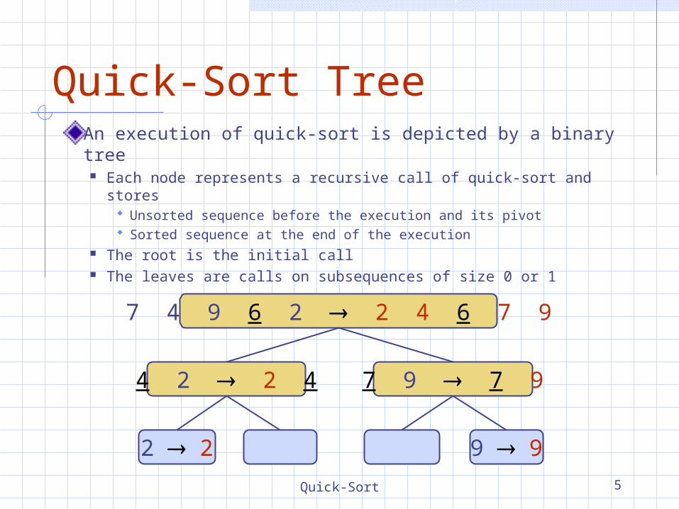
Quick-Sort TreeAn execution of quick-sort is depicted by a binary tree

Each node represents a recursive call of quick-sort and stores Unsorted sequence before the execution and its pivot Sorted sequence at the end of the execution

The root is the initial call The leaves are calls on subsequences of size 0 or 1

7 4 9 6 2 2 4 6 7 9

4 2 2 4 7 9 7 9

2 2 9 9

Quick-Sort 6

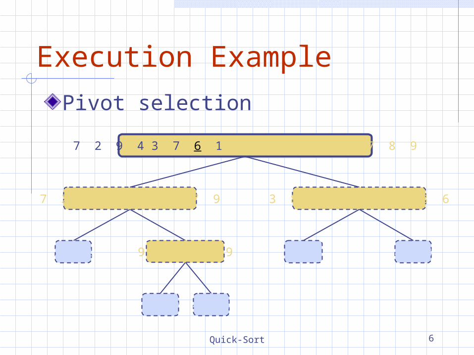
Execution Example

Pivot selection

7 2 9 4 2 4 7 9

2 2

7 2 9 4 3 7 6 1 1 2 3 4 6 7 8 9

3 8 6 1 1 3 8 6

3 3 8 89 4 4 9

9 9 4 4

Quick-Sort 7

Execution Example (cont.)Partition, recursive call, pivot selection

2 4 3 1 2 4 7 9

9 4 4 9

9 9 4 4

7 2 9 4 3 7 6 1 1 2 3 4 6 7 8 9

3 8 6 1 1 3 8 6

3 3 8 82 2

Quick-Sort 8

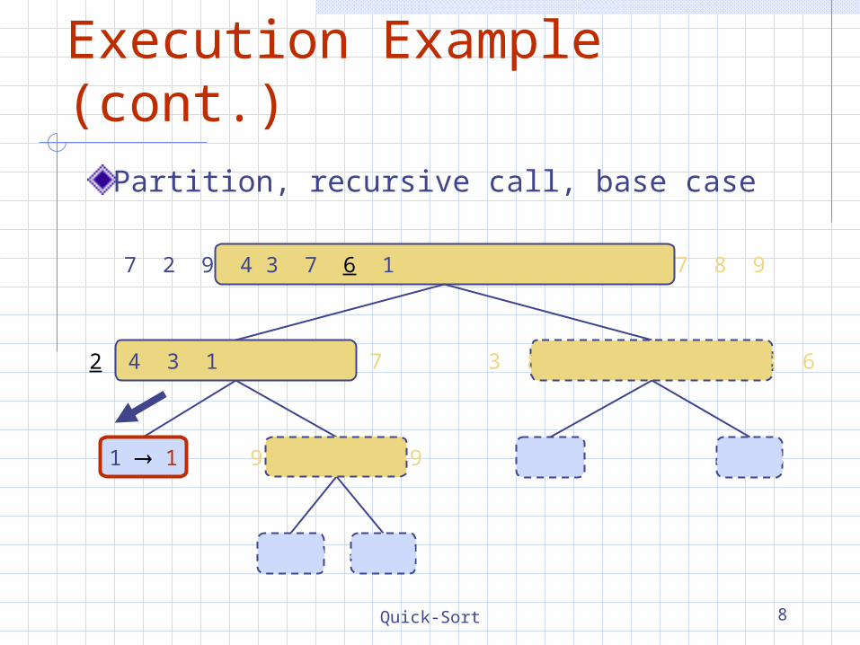
Execution Example (cont.)

Partition, recursive call, base case

2 4 3 1 2 4 7

1 1 9 4 4 9

9 9 4 4

7 2 9 4 3 7 6 1 1 2 3 4 6 7 8 9

3 8 6 1 1 3 8 6

3 3 8 8

Quick-Sort 9

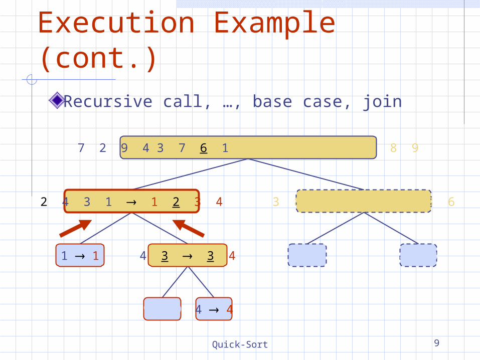
Execution Example (cont.)

Recursive call, …, base case, join

3 8 6 1 1 3 8 6

3 3 8 8

7 2 9 4 3 7 6 1 1 2 3 4 6 7 8 9

2 4 3 1 1 2 3 4

1 1 4 3 3 4

9 9 4 4

Quick-Sort 10

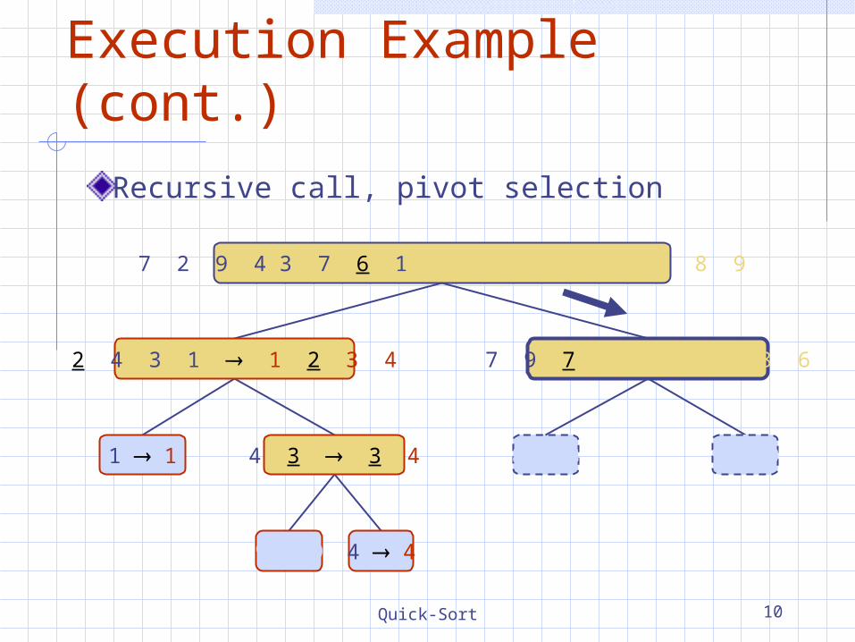
Execution Example (cont.)

Recursive call, pivot selection

7 9 7 1 1 3 8 6

8 8

7 2 9 4 3 7 6 1 1 2 3 4 6 7 8 9

2 4 3 1 1 2 3 4

1 1 4 3 3 4

9 9 4 4

9 9

Quick-Sort 11

Execution Example (cont.)Partition, …, recursive call, base case

7 9 7 1 1 3 8 6

8 8

7 2 9 4 3 7 6 1 1 2 3 4 6 7 8 9

2 4 3 1 1 2 3 4

1 1 4 3 3 4

9 9 4 4

9 9

Quick-Sort 12

Execution Example (cont.)

Join, join

7 9 7 17 7 9

8 8

7 2 9 4 3 7 6 1 1 2 3 4 6 7 7 9

2 4 3 1 1 2 3 4

1 1 4 3 3 4

9 9 4 4

9 9

Quick-Sort 13

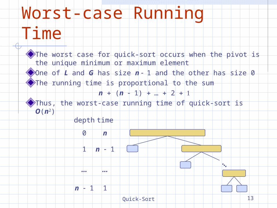
Worst-case Running TimeThe worst case for quick-sort occurs when the pivot is the unique minimum or maximum elementOne of L and G has size n 1 and the other has size 0The running time is proportional to the sum

n (n 1) … 2 Thus, the worst-case running time of quick-sort is O(n2)

depth time

0 n

1 n 1

… …

n 1 1

…

Quick-Sort 14

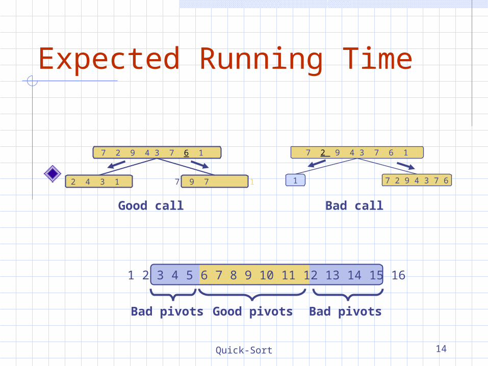
Expected Running Time

7 9 7 1 1

7 2 9 4 3 7 6 1 9

2 4 3 1 7 2 9 4 3 7 61

7 2 9 4 3 7 6 1

Good call Bad call

1 2 3 4 5 6 7 8 9 10 11 12 13 14 15 16

Good pivotsBad pivots Bad pivots

Quick-Sort 15

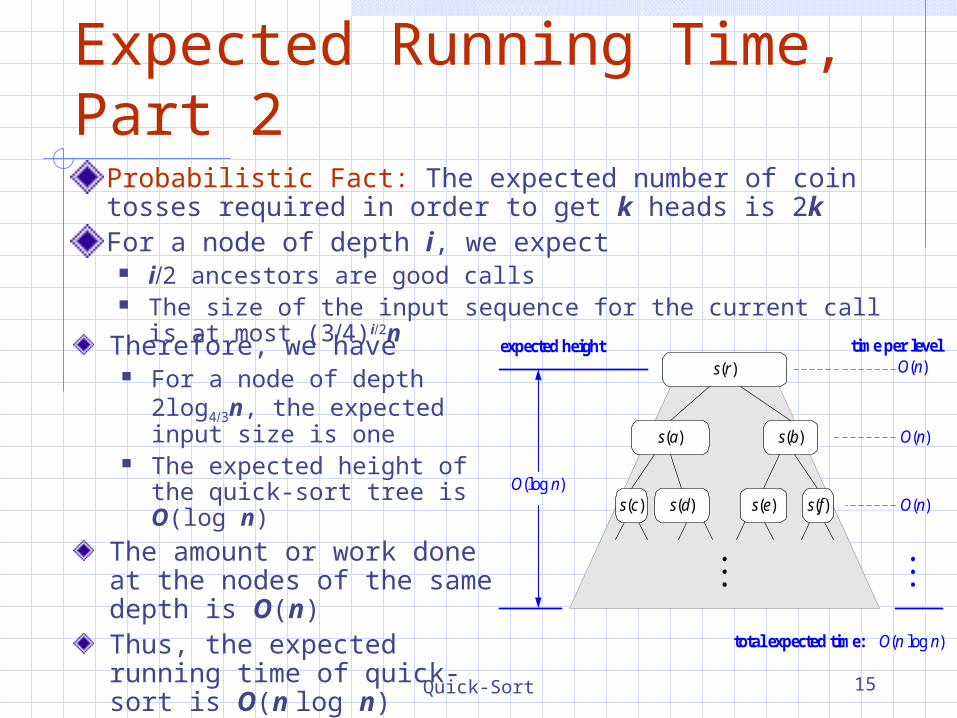
Expected Running Time, Part 2

Probabilistic Fact: The expected number of coin tosses required in order to get k heads is 2kFor a node of depth i, we expect

i2 ancestors are good calls The size of the input sequence for the current call is at most

(34)i2ns(r)

s(a) s(b)

s(c) s(d) s(f)s(e)

time per levelexpected height

O(log n)

O(n)

O(n)

O(n)

total expected time: O(n log n)

Therefore, we have For a node of depth 2log43n,

the expected input size is one

The expected height of the quick-sort tree is O(log n)

The amount or work done at the nodes of the same depth is O(n)Thus, the expected running time of quick-sort is O(n log n)

Quick-Sort 16

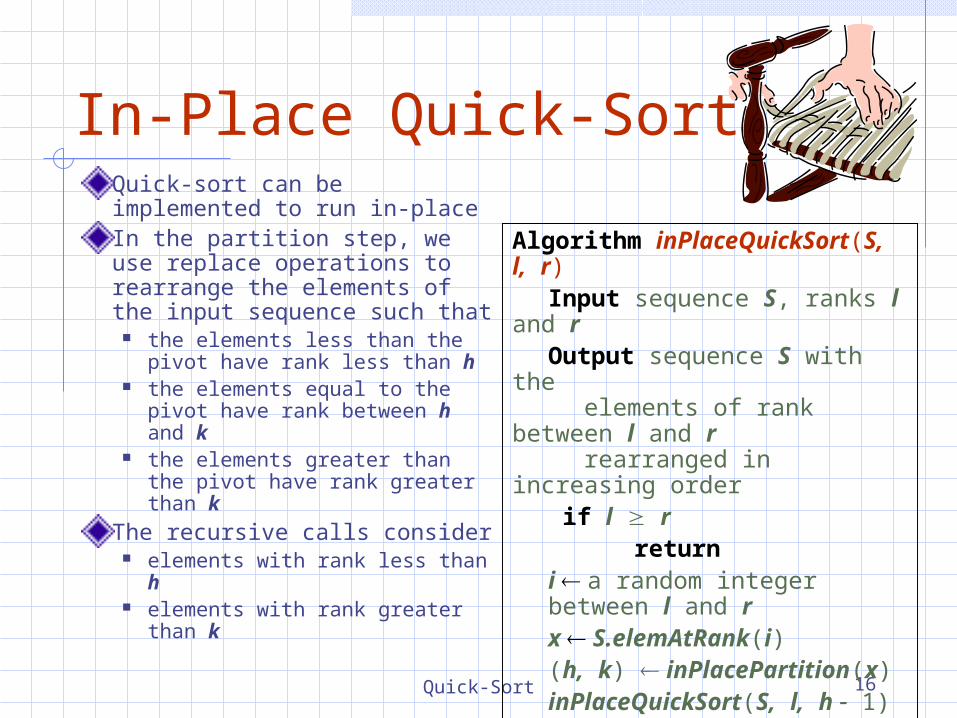
In-Place Quick-SortQuick-sort can be implemented to run in-placeIn the partition step, we use replace operations to rearrange the elements of the input sequence such that

the elements less than the pivot have rank less than h

the elements equal to the pivot have rank between h and k

the elements greater than the pivot have rank greater than k

The recursive calls consider elements with rank less than h elements with rank greater

than k

Algorithm inPlaceQuickSort(S, l, r)Input sequence S, ranks l and rOutput sequence S with the

elements of rank between l and rrearranged in increasing order

if l r return

i a random integer between l and r x S.elemAtRank(i) (h, k) inPlacePartition(x)inPlaceQuickSort(S, l, h 1)inPlaceQuickSort(S, k 1, r)

Quick-Sort 17

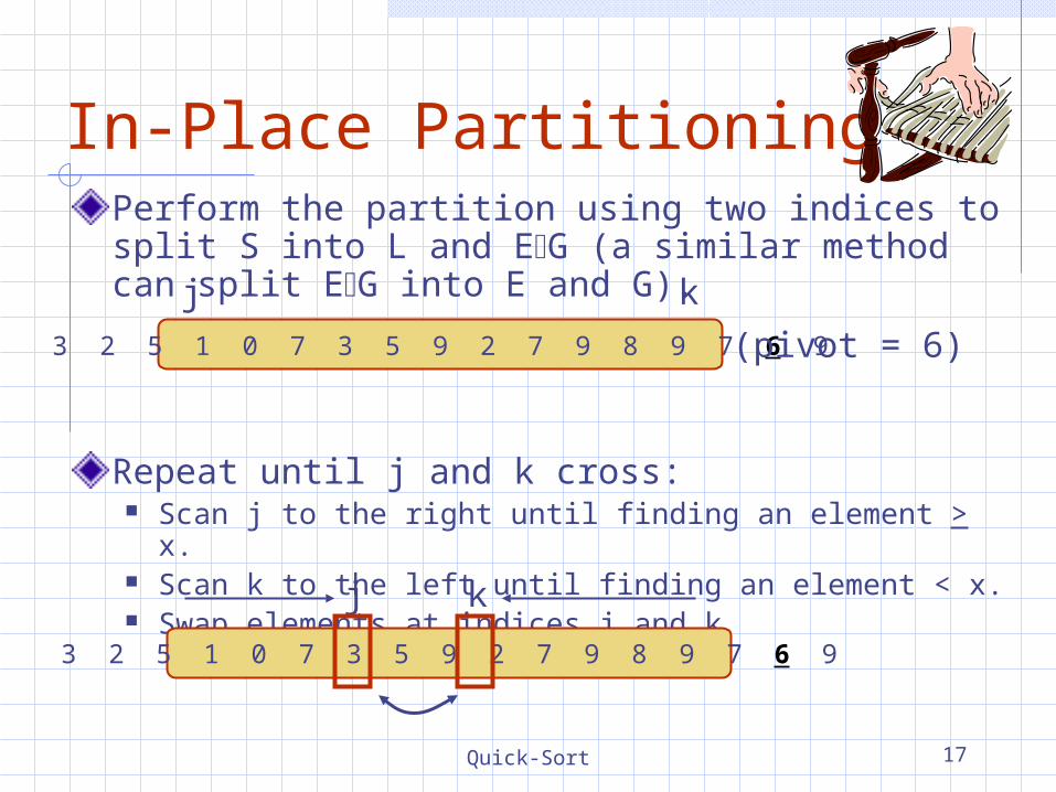
In-Place PartitioningPerform the partition using two indices to split S into L and EG (a similar method can split EG into E and G).

Repeat until j and k cross: Scan j to the right until finding an element > x. Scan k to the left until finding an element < x. Swap elements at indices j and k

3 2 5 1 0 7 3 5 9 2 7 9 8 9 7 6 9

j k

(pivot = 6)

3 2 5 1 0 7 3 5 9 2 7 9 8 9 7 6 9

j k

Quick-Sort 18

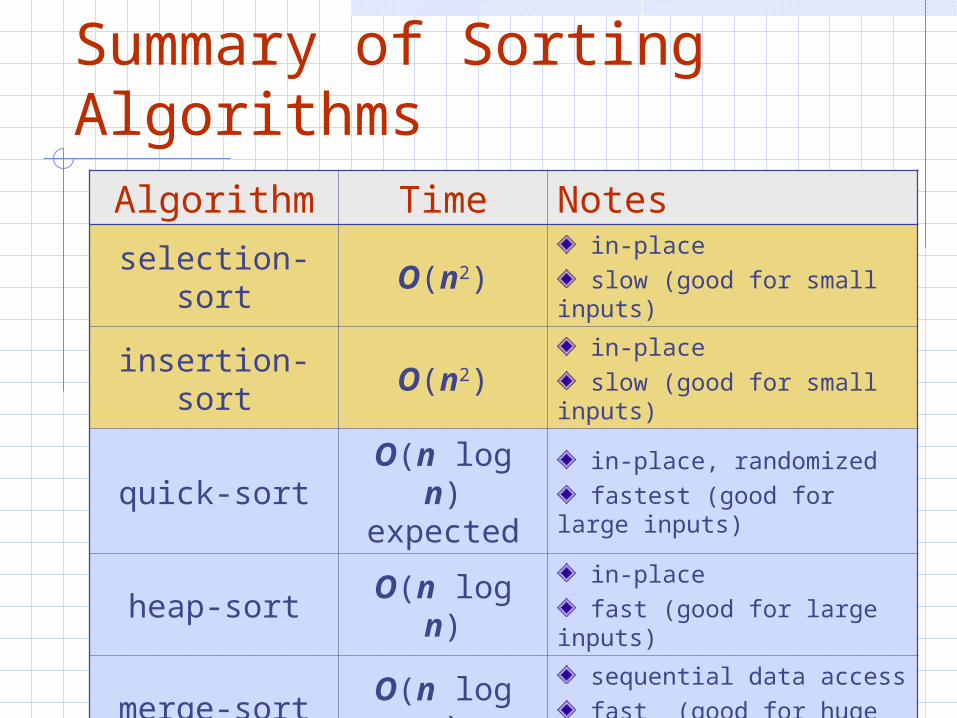
Summary of Sorting Algorithms

Algorithm Time Notes

selection-sort O(n2) in-place slow (good for small

inputs)

insertion-sort O(n2) in-place slow (good for small

inputs)

quick-sortO(n log n)expected

in-place, randomized fastest (good for large

inputs)

heap-sort O(n log n) in-place fast (good for large inputs)

merge-sort O(n log n) sequential data access fast (good for huge

inputs)