quantum transport through double-dot aharonov-bohm ... · quantum transport through double-dot...
TRANSCRIPT
Quantum transport through double-dot Aharonov-Bohm
interferometers
by
Salil Bedkihal
A thesis submitted in conformity with the requirementsfor the degree of Doctor of PhilosophyGraduate Department of Chemistry
University of Toronto
c© Copyright 2014 by Salil Bedkihal
Abstract
Quantum transport through double-dot Aharonov-Bohm interferometers
Salil Bedkihal
Doctor of Philosophy
Graduate Department of Chemistry
University of Toronto
2014
Understanding the interplay of nonequilibrium effects, dissipation and many body in-
teractions is a fundamental challenge in condensed matter physics. In this thesis, as
a case study, we focus on the transient dynamics and the steady state characterstics
of the double-dot Aharonov-Bohm (AB) interferometer subjected to a voltage and/or
temperature bias.
We first consider an exactly solvable case, the noninteracting double-dot AB interfer-
ometer. The transient dynamics of this model is studied using an exact fermionic trace
formula, and the analytic expressions in the long time limit are obtained using a nonequi-
librium Green’s function technique. We also study the effects of elastic dephasing on the
occupation-flux behaviour in this noninteracting limit. Several nontrivial magnetic flux
control effects are exposed, potentially useful for the design of nanoscale devices.
The real time dynamics of the coherences and the charge current in an interact-
ing interferometer is simulated using the numerically exact influence functional path
integral (INFPI) technique. The temporal characterstics of the coherence in the weak-
intermediate Coulomb repulsion case are qualitatively similar to those found in the non-
interacting limit. In contrast, in the large Coulomb repulsion and the large bias limit,
master equation simulations reveal notably different dynamics and steady state charac-
terstics.
We study the effects of many body interactions on magnetoasymmetries of nonlin-
ii
ear transport coefficients using phenomenological models, Buttiker’s probes. Sufficient
conditions for the diode functionality in Aharonov-Bohm interferometers are obtained
analytically within the framework of Landauer-Buttiker scattering theory. Predictions of
the phenomenological probes models are verified by studying a microscopic model with
a genuine many body interaction, a double-dot interferometer capacitively coupled to a
fermionic environment. These simulations are carried out using the INFPI technique.
Some general comments about the suitability of INFPI to study nonlinear transport are
presented. This work could be extended to explore nonlinear thermoelectric transport
and diode behaviour in interacting many body systems.
iii

Dedication
I would like to dedicate this thesis to my mother Savita who is not living now. She
motivated me to learn science, and especially Physics.
Acknowledgements
I would like to sincerely acknowledge all those people who made this work possible. My
first acknowledgement goes to my supervisor Prof. Dvira Segal for her inexorable support.
She always gave me space and time to implement my own ideas. I am very grateful to
my supervisory committee members, Prof. Kapral, Prof. Scholes, Prof. Artur Izmaylov
and Prof. Dhirani for their critical comments and interesting questions. I would like to
acknowledge Prof. George Kirczenow at the Simon Fraser University for critical feedback
and interesting questions on my work.
This work would not have been possible without my family. I am very thankful to my
father for his emotional support. He always motivated me to pursue scientific research,
and provided an infrastructural support so that I could concentrate on my work. I am
highly indebted to my aunt Sharmila, uncle Sudhir, cousin Neeraja, grandparents Usha
and Aaba for their emotional and moral support during this work. Dinner was always
ready and I never had to eat outside; grandparent’s special Kolhapuri spicy delight has
fueled my scientific imagination. Also my aunt’s special chai tea has kept me awake,
especially when sleepless nights with tedious Green’s function calculations were the inte-
gral part of my life. I would like to acknowledge my poetic friend Pramod Koparde for
his constant encouragement and support.
Friends and colleagues have played an important role in shaping my personal and
acdemic growth. I am very thankful to my friends Inga, Darcy, Louis, Anand, Subodh,
Manisha for their support. This work would not have been possible without pubnights
and beer parties with my friends. I acknowledge and appreciate support from my col-
iv
leagues Cyrille Lavigne, Lena Simine, Malay Bandyopadhyay, Claire Wu, Savanah Gar-
mon, Crystal Chen, and Dr. Aurelia Chenu . We discussed various topics pertaining
to open quantum systems which turned out to be particularly useful while reassembling
my work into a thesis. I am also very thankful to Prof. Bill Coish, Benjamin D’Anjou
at McGill’s Physics department, Prof. Rajeev Pathak and Prof. P Durganandini at
University of Pune department of Physics India for interesting discussions and critical
comments on my work. I am very beholden to Dr. Rainer Hartle for discussions and
critical comments during the APS March meetings, 2013 and 2014.
I would like to thank all the members of the Chemical Physics Theory Group for
their support and feedback. Finally I am very grateful to the Department of Chemistry,
University of Toronto, for providing me an opportunity to pursue graduate studies, and
special thanks to Anna Liza for an excellent administrative support.
I gratefully acknowledge funding support from the Department of Chemistry Univer-
sity of Toronto, Queen-Elizabeth II/Martin Moskovits Scholarship in Science and Tech-
nology, the Lachlan Gilchrist Fellowship Fund, Michael Dignam Travel Award, Donald
J. LeRoy Prize, and NSERC.
Finally, I would like to thank the American Physical Society and European Physical
Society, for authorization to include in my thesis the material which was previously
published in Physical Review B and European Physical Journal B: Phys. Rev. B 88,
155407, (2013), Phys. Rev. B 87, 045418, (2013), Phys. Rev. B 85, 155324, (2012), and
Eur. Phys. J. B 86, 503, (2013).
v
Contents
1 Introduction 1
1.1 Aharonov-Bohm effect . . . . . . . . . . . . . . . . . . . . . . . . . . . . 1
1.2 Motivation . . . . . . . . . . . . . . . . . . . . . . . . . . . . . . . . . . . 3
2 Double-dot Aharonov-Bohm interferometer 11
2.1 Models . . . . . . . . . . . . . . . . . . . . . . . . . . . . . . . . . . . . . 11
2.2 Observables and methods . . . . . . . . . . . . . . . . . . . . . . . . . . 16
2.3 Open questions . . . . . . . . . . . . . . . . . . . . . . . . . . . . . . . . 34
3 Model I: Noninteracting electrons 41
3.1 Introduction . . . . . . . . . . . . . . . . . . . . . . . . . . . . . . . . . . 41
3.2 Equations of motion . . . . . . . . . . . . . . . . . . . . . . . . . . . . . 41
3.3 Stationary behaviour . . . . . . . . . . . . . . . . . . . . . . . . . . . . . 45
3.4 Transient behavior . . . . . . . . . . . . . . . . . . . . . . . . . . . . . . 57
3.5 Dephasing . . . . . . . . . . . . . . . . . . . . . . . . . . . . . . . . . . . 59
3.6 Discussion . . . . . . . . . . . . . . . . . . . . . . . . . . . . . . . . . . . 64
4 Model I interacting case: Coherence dynamics 65
4.1 Introduction . . . . . . . . . . . . . . . . . . . . . . . . . . . . . . . . . . 65
4.2 Model I . . . . . . . . . . . . . . . . . . . . . . . . . . . . . . . . . . . . 66
4.3 INFPI numerical results . . . . . . . . . . . . . . . . . . . . . . . . . . . 68
vi
4.4 Master equation analysis: U = 0 and U = ∞ . . . . . . . . . . . . . . . . 77
4.5 Discussion . . . . . . . . . . . . . . . . . . . . . . . . . . . . . . . . . . . 79
5 Symmetries of nonlinear transport 82
5.1 Introduction . . . . . . . . . . . . . . . . . . . . . . . . . . . . . . . . . . 82
5.2 Symmetry measures and main results . . . . . . . . . . . . . . . . . . . . 84
5.3 Phase rigidity and absence of rectification . . . . . . . . . . . . . . . . . 88
5.4 Beyond linear response: spatially symmetric setups . . . . . . . . . . . . 93
5.5 Beyond linear response: model II . . . . . . . . . . . . . . . . . . . . . . 95
5.6 Numerical simulations . . . . . . . . . . . . . . . . . . . . . . . . . . . . 99
5.7 Relation of results to other treatments . . . . . . . . . . . . . . . . . . . 115
5.8 Discussion . . . . . . . . . . . . . . . . . . . . . . . . . . . . . . . . . . . 117
6 Microscopic approach: model III 120
6.1 Introduction . . . . . . . . . . . . . . . . . . . . . . . . . . . . . . . . . . 120
6.2 Model . . . . . . . . . . . . . . . . . . . . . . . . . . . . . . . . . . . . . 120
6.3 Numerical results . . . . . . . . . . . . . . . . . . . . . . . . . . . . . . . 122
6.4 Discussion . . . . . . . . . . . . . . . . . . . . . . . . . . . . . . . . . . . 127
7 Conclusions and future directions 129
7.1 Summary . . . . . . . . . . . . . . . . . . . . . . . . . . . . . . . . . . . 129
7.2 Observations . . . . . . . . . . . . . . . . . . . . . . . . . . . . . . . . . . 131
7.3 Future work . . . . . . . . . . . . . . . . . . . . . . . . . . . . . . . . . . 134
vii
List of Figures
1.1 Aharonov-Bohm interferometer with magnetic flux Φ. . . . . . . . . . . . 2
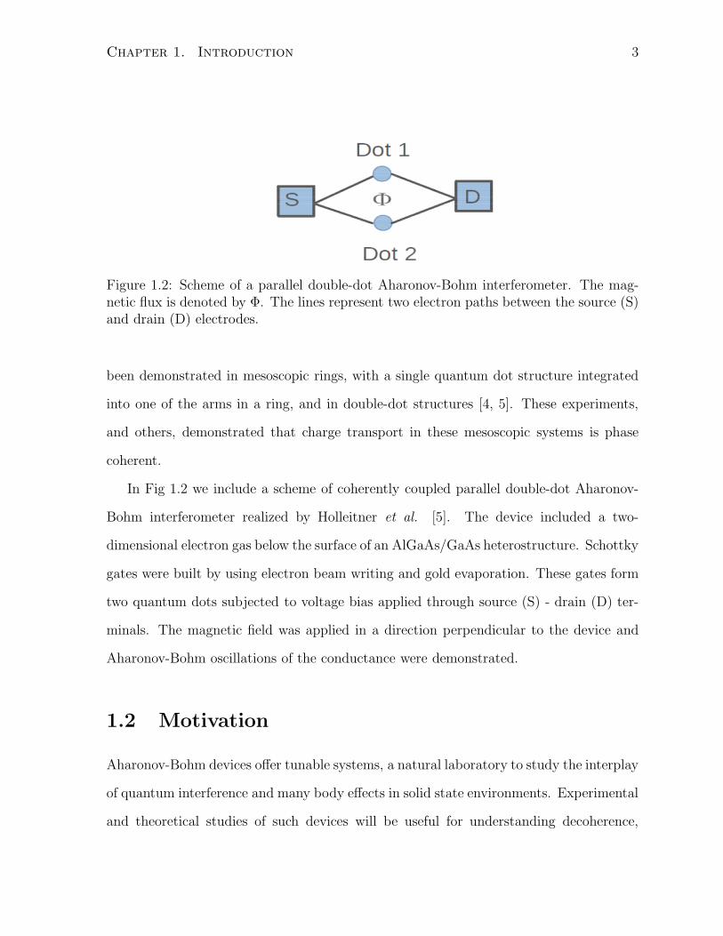
1.2 Scheme of a parallel double-dot Aharonov-Bohm interferometer. The mag-
netic flux is denoted by Φ. The lines represent two electron paths between
the source (S) and drain (D) electrodes. . . . . . . . . . . . . . . . . . . . 3
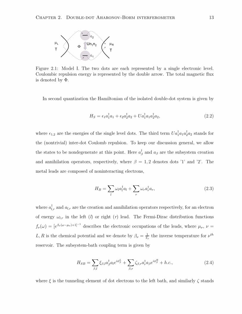
2.1 Model I. The two dots are each represented by a single electronic level.
Coulombic repulsion energy is represented by the double arrow. The total
magnetic flux is denoted by Φ. . . . . . . . . . . . . . . . . . . . . . . . . 13
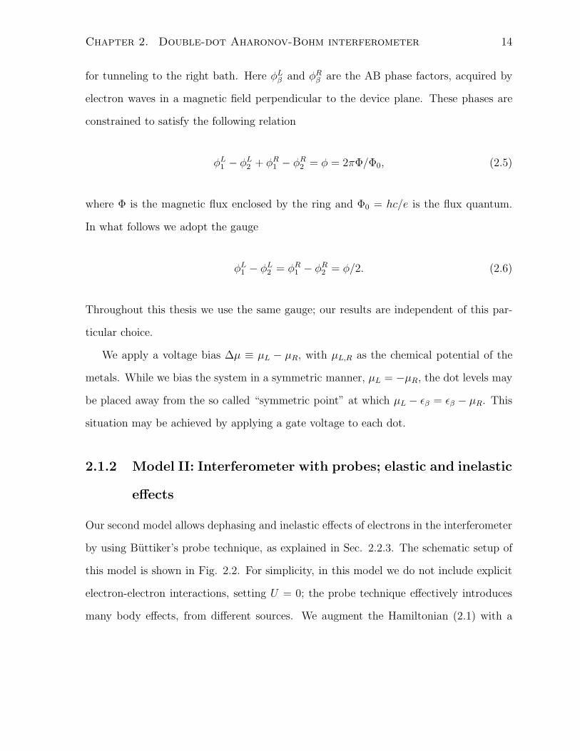
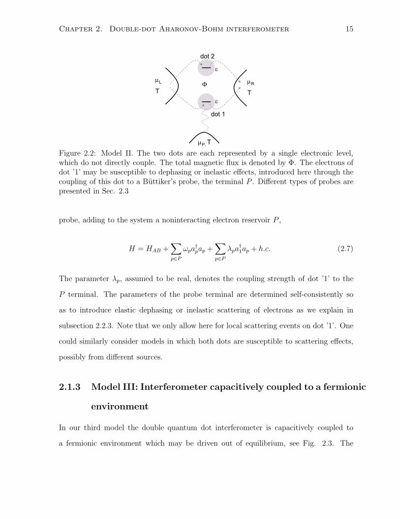
2.2 Model II. The two dots are each represented by a single electronic level,
which do not directly couple. The total magnetic flux is denoted by Φ.
The electrons of dot ’1’ may be susceptible to dephasing or inelastic effects,
introduced here through the coupling of this dot to a Buttiker’s probe, the
terminal P . Different types of probes are presented in Sec. 2.3 . . . . . . 15
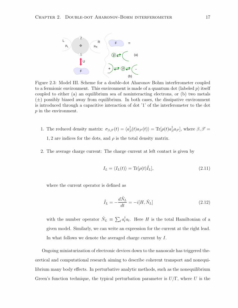
2.3 Model III. Scheme for a double-dot Aharonov Bohm interferometer cou-
pled to a fermionic environment. This environment is made of a quantum
dot (labeled p) itself coupled to either (a) an equilibrium sea of noninter-
acting electrons, or (b) two metals (±) possibly biased away from equilib-
rium. In both cases, the dissipative environment is introduced through a
capacitive interaction of dot ’1’ of the interferometer to the dot p in the
environment. . . . . . . . . . . . . . . . . . . . . . . . . . . . . . . . . . 17
viii
3.1 (a) Flux dependency of occupation for dot ’1’ using ǫ = 0 (triangle) ǫ = 0.2
(�) ǫ = 0.3 (◦), ǫ = 0.35 (⋆) and ǫ = 0.4 (+). Panel (b) displays results
when ǫ is tuned to the bias window edge, ǫ ∼ µL, ǫ = 0.29 (�), ǫ = 0.3
(diagonal), ǫ = 0.31 (◦), and ǫ = 0.31, T = 0.05 (dashed-dotted line). In
all cases µL = −µR = 0.3, γ = 0.05, and T = 0, unless otherwise stated.
Reproduced from Ref. [115]. . . . . . . . . . . . . . . . . . . . . . . . . . 49
3.2 (a)-(b) Dots occupations as a function of magnetic phase φ for ∆µ = 0.6,
ǫ = 0.2, T = 0. (c) Occupation difference, δn = σ1,1 − σ2,2. At weak
coupling, γ = 0.05 (△), the dots occupations are almost identical. When
the hybridization is made stronger, γ = 0.5 (◦), comparable to the levels
displacement from the symmetric point, σ1,1 clearly deviates from σ2,2.
At very strong coupling, γ = 2 (+), the occupation difference reduces and
asymmetries develop. For clarity, results are shown for φ/π between (-2,2).
Reproduced from Ref [115]. . . . . . . . . . . . . . . . . . . . . . . . . . 49
3.3 Occupation difference as a function of bias voltage ∆µ, for different mag-
netic flux values, φ = π/2 (full line), φ = π/4 (dashed line), φ = π/8
(dashed-dotted line). Other parameters are ǫ = 0.2 and γ = 0.05, Tν = 0.
The inset presents data for backward and forward biases; the main plot
zooms on the positive bias regime. Reproduced from Ref. [115]. . . . . . 51
3.4 Occupation difference as a function of magnetic flux for different bias val-
ues, ∆µ = 0.1 (full line), ∆µ = 0.2 (dashed line), ∆µ = 0.3 (dashed-dotted
line) and ∆µ = 0.4 (dotted line). Other parameters are ǫ = 0.2, γ = 0.05
and Tν = 0. Reproduced from Ref. [115]. . . . . . . . . . . . . . . . . . . 51
ix
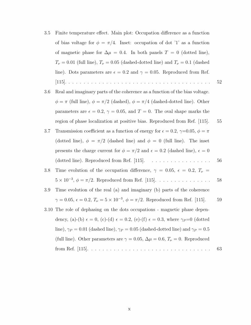
3.5 Finite temperature effect. Main plot: Occupation difference as a function
of bias voltage for φ = π/4. Inset: occupation of dot ’1’ as a function
of magnetic phase for ∆µ = 0.4. In both panels T = 0 (dotted line),
Tν = 0.01 (full line), Tν = 0.05 (dashed-dotted line) and Tν = 0.1 (dashed
line). Dots parameters are ǫ = 0.2 and γ = 0.05. Reproduced from Ref.
[115]. . . . . . . . . . . . . . . . . . . . . . . . . . . . . . . . . . . . . . . 52
3.6 Real and imaginary parts of the coherence as a function of the bias voltage.
φ = π (full line), φ = π/2 (dashed), φ = π/4 (dashed-dotted line). Other
parameters are ǫ = 0.2, γ = 0.05, and T = 0. The oval shape marks the
region of phase localization at positive bias. Reproduced from Ref. [115]. 55
3.7 Transmission coefficient as a function of energy for ǫ = 0.2, γ=0.05, φ = π
(dotted line), φ = π/2 (dashed line) and φ = 0 (full line). The inset
presents the charge current for φ = π/2 and ǫ = 0.2 (dashed line), ǫ = 0
(dotted line). Reproduced from Ref. [115]. . . . . . . . . . . . . . . . . 56
3.8 Time evolution of the occupation difference, γ = 0.05, ǫ = 0.2, Tν =
5× 10⁻³, φ = π/2. Reproduced from Ref. [115]. . . . . . . . . . . . . . . 58
3.9 Time evolution of the real (a) and imaginary (b) parts of the coherence
γ = 0.05, ǫ = 0.2, Tν = 5× 10⁻³, φ = π/2. Reproduced from Ref. [115]. 59
3.10 The role of dephasing on the dots occupations - magnetic phase depen-
dency, (a)-(b) ǫ = 0, (c)-(d) ǫ = 0.2, (e)-(f) ǫ = 0.3, where γP=0 (dotted
line), γP = 0.01 (dashed line), γP = 0.05 (dashed-dotted line) and γP = 0.5
(full line). Other parameters are γ = 0.05, ∆µ = 0.6, Tν = 0. Reproduced
from Ref. [115]. . . . . . . . . . . . . . . . . . . . . . . . . . . . . . . . . 63
x
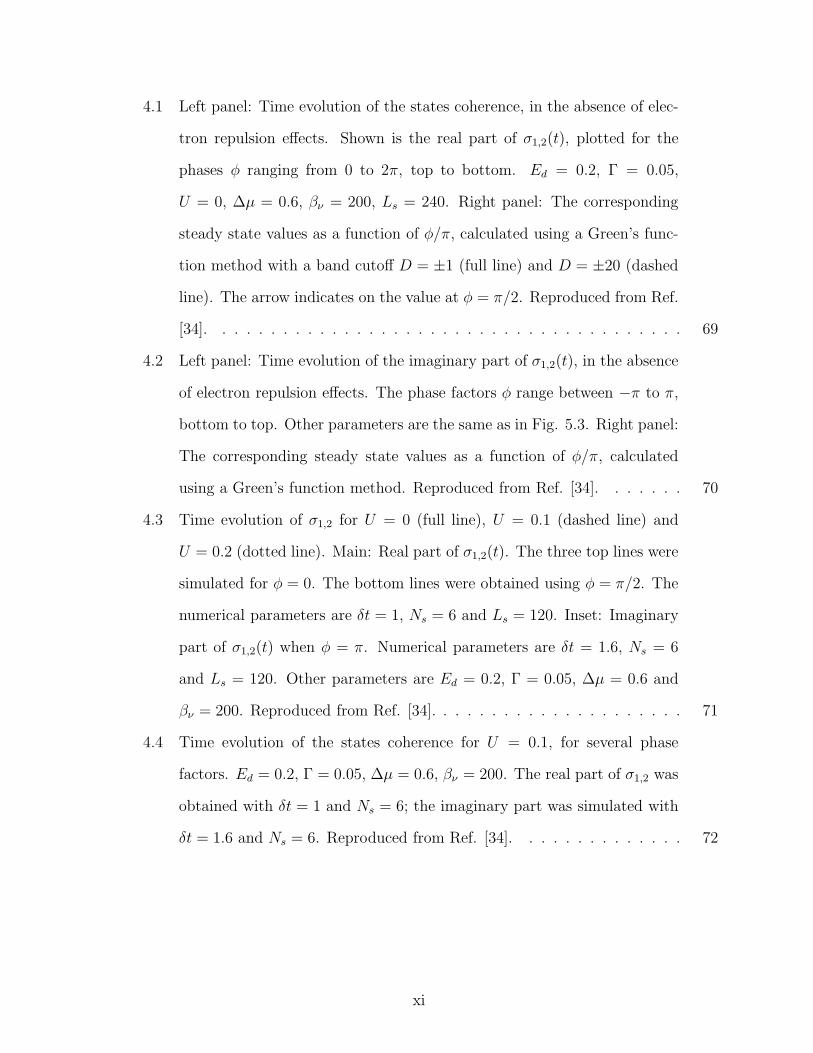
4.1 Left panel: Time evolution of the states coherence, in the absence of elec-
tron repulsion effects. Shown is the real part of σ1,2(t), plotted for the
phases φ ranging from 0 to 2π, top to bottom. Ed = 0.2, Γ = 0.05,
U = 0, ∆µ = 0.6, βν = 200, Ls = 240. Right panel: The corresponding
steady state values as a function of φ/π, calculated using a Green’s func-
tion method with a band cutoff D = ±1 (full line) and D = ±20 (dashed
line). The arrow indicates on the value at φ = π/2. Reproduced from Ref.
[34]. . . . . . . . . . . . . . . . . . . . . . . . . . . . . . . . . . . . . . . 69
4.2 Left panel: Time evolution of the imaginary part of σ1,2(t), in the absence
of electron repulsion effects. The phase factors φ range between −π to π,
bottom to top. Other parameters are the same as in Fig. 5.3. Right panel:
The corresponding steady state values as a function of φ/π, calculated
using a Green’s function method. Reproduced from Ref. [34]. . . . . . . 70
4.3 Time evolution of σ1,2 for U = 0 (full line), U = 0.1 (dashed line) and
U = 0.2 (dotted line). Main: Real part of σ1,2(t). The three top lines were
simulated for φ = 0. The bottom lines were obtained using φ = π/2. The
numerical parameters are δt = 1, Ns = 6 and Ls = 120. Inset: Imaginary
part of σ1,2(t) when φ = π. Numerical parameters are δt = 1.6, Ns = 6
and Ls = 120. Other parameters are Ed = 0.2, Γ = 0.05, ∆µ = 0.6 and
βν = 200. Reproduced from Ref. [34]. . . . . . . . . . . . . . . . . . . . . 71
4.4 Time evolution of the states coherence for U = 0.1, for several phase
factors. Ed = 0.2, Γ = 0.05, ∆µ = 0.6, βν = 200. The real part of σ1,2 was
obtained with δt = 1 and Ns = 6; the imaginary part was simulated with
δt = 1.6 and Ns = 6. Reproduced from Ref. [34]. . . . . . . . . . . . . . 72
xi
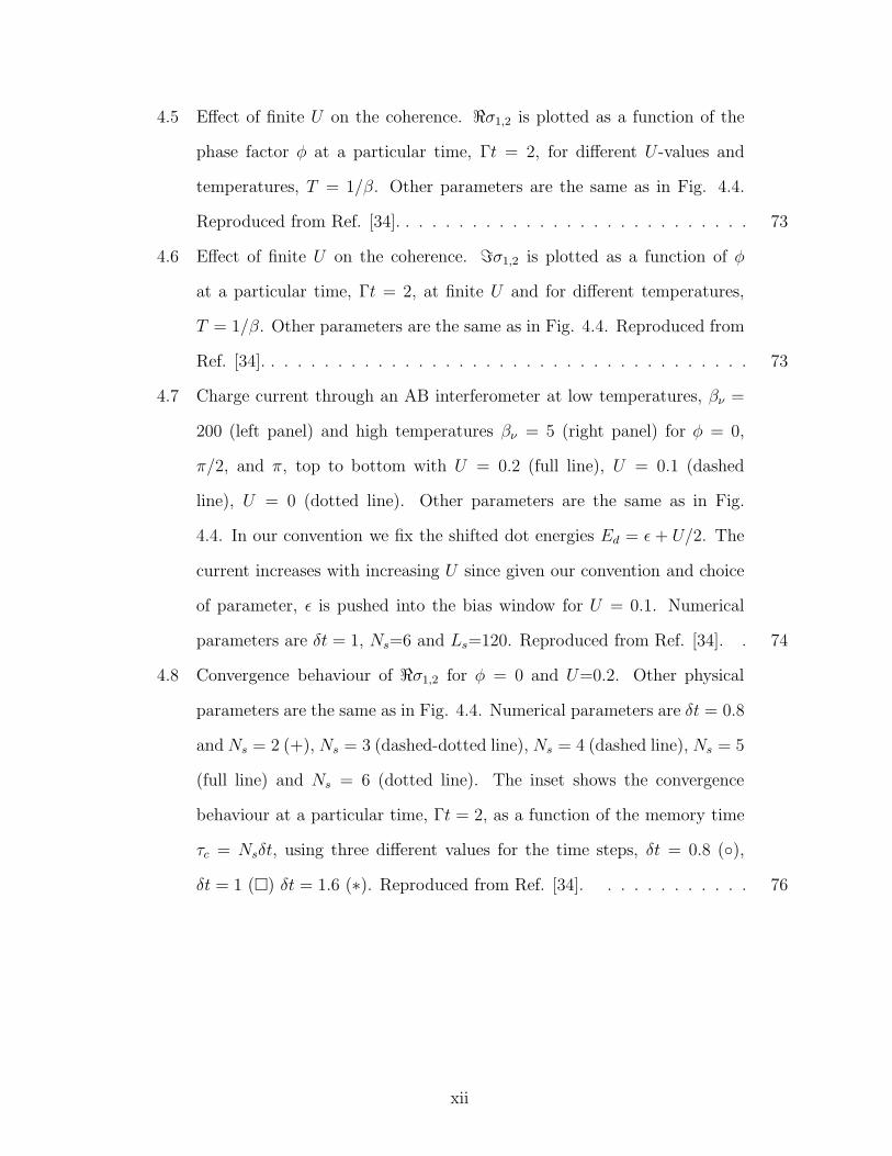
4.5 Effect of finite U on the coherence. ℜσ1,2 is plotted as a function of the
phase factor φ at a particular time, Γt = 2, for different U -values and
temperatures, T = 1/β. Other parameters are the same as in Fig. 4.4.
Reproduced from Ref. [34]. . . . . . . . . . . . . . . . . . . . . . . . . . . 73
4.6 Effect of finite U on the coherence. ℑσ1,2 is plotted as a function of φ
at a particular time, Γt = 2, at finite U and for different temperatures,
T = 1/β. Other parameters are the same as in Fig. 4.4. Reproduced from
Ref. [34]. . . . . . . . . . . . . . . . . . . . . . . . . . . . . . . . . . . . . 73
4.7 Charge current through an AB interferometer at low temperatures, βν =
200 (left panel) and high temperatures βν = 5 (right panel) for φ = 0,
π/2, and π, top to bottom with U = 0.2 (full line), U = 0.1 (dashed
line), U = 0 (dotted line). Other parameters are the same as in Fig.
4.4. In our convention we fix the shifted dot energies Ed = ǫ + U/2. The
current increases with increasing U since given our convention and choice
of parameter, ǫ is pushed into the bias window for U = 0.1. Numerical
parameters are δt = 1, Ns=6 and Ls=120. Reproduced from Ref. [34]. . 74
4.8 Convergence behaviour of ℜσ1,2 for φ = 0 and U=0.2. Other physical
parameters are the same as in Fig. 4.4. Numerical parameters are δt = 0.8
andNs = 2 (+), Ns = 3 (dashed-dotted line), Ns = 4 (dashed line), Ns = 5
(full line) and Ns = 6 (dotted line). The inset shows the convergence
behaviour at a particular time, Γt = 2, as a function of the memory time
τc = Nsδt, using three different values for the time steps, δt = 0.8 (◦),
δt = 1 (�) δt = 1.6 (∗). Reproduced from Ref. [34]. . . . . . . . . . . . 76
xii
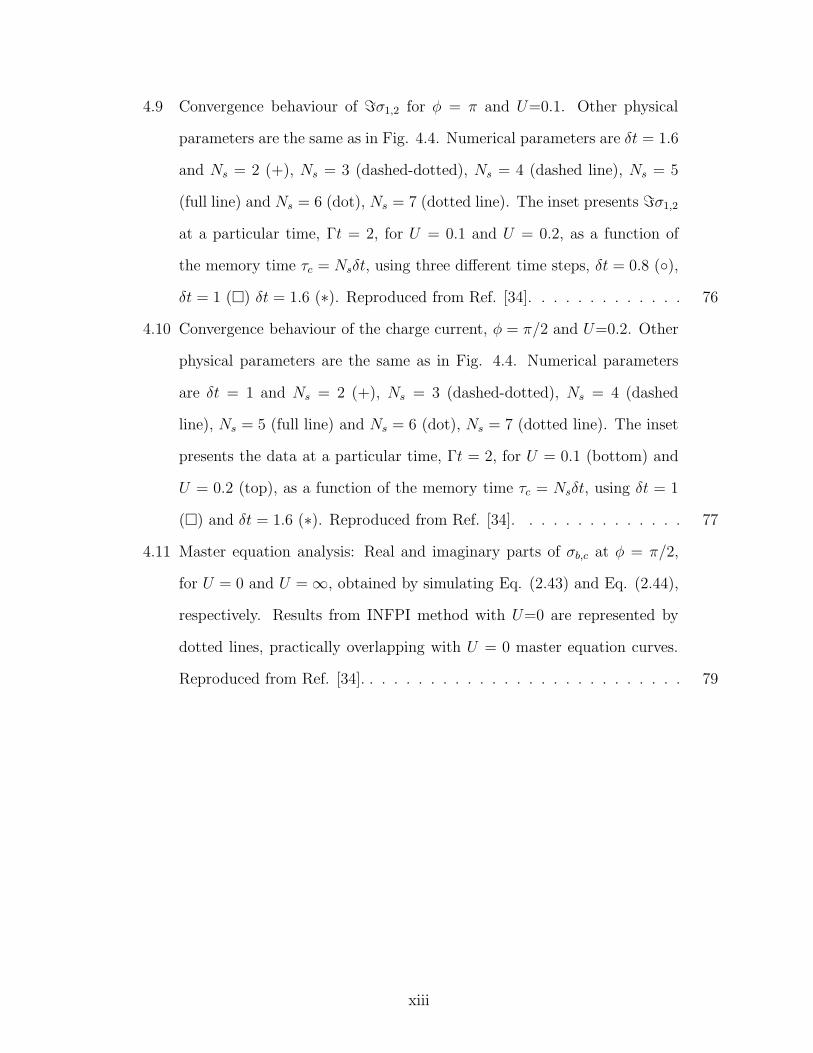
4.9 Convergence behaviour of ℑσ1,2 for φ = π and U=0.1. Other physical
parameters are the same as in Fig. 4.4. Numerical parameters are δt = 1.6
and Ns = 2 (+), Ns = 3 (dashed-dotted), Ns = 4 (dashed line), Ns = 5
(full line) and Ns = 6 (dot), Ns = 7 (dotted line). The inset presents ℑσ1,2
at a particular time, Γt = 2, for U = 0.1 and U = 0.2, as a function of
the memory time τc = Nsδt, using three different time steps, δt = 0.8 (◦),
δt = 1 (�) δt = 1.6 (∗). Reproduced from Ref. [34]. . . . . . . . . . . . . 76
4.10 Convergence behaviour of the charge current, φ = π/2 and U=0.2. Other
physical parameters are the same as in Fig. 4.4. Numerical parameters
are δt = 1 and Ns = 2 (+), Ns = 3 (dashed-dotted), Ns = 4 (dashed
line), Ns = 5 (full line) and Ns = 6 (dot), Ns = 7 (dotted line). The inset
presents the data at a particular time, Γt = 2, for U = 0.1 (bottom) and
U = 0.2 (top), as a function of the memory time τc = Nsδt, using δt = 1
(�) and δt = 1.6 (∗). Reproduced from Ref. [34]. . . . . . . . . . . . . . 77
4.11 Master equation analysis: Real and imaginary parts of σb,c at φ = π/2,
for U = 0 and U = ∞, obtained by simulating Eq. (2.43) and Eq. (2.44),
respectively. Results from INFPI method with U=0 are represented by
dotted lines, practically overlapping with U = 0 master equation curves.
Reproduced from Ref. [34]. . . . . . . . . . . . . . . . . . . . . . . . . . . 79
xiii
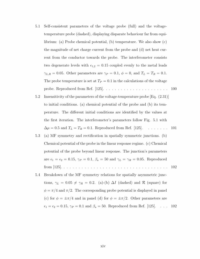
5.1 Self-consistent parameters of the voltage probe (full) and the voltage-
temperature probe (dashed), displaying disparate behaviour far from equi-
librium: (a) Probe chemical potential, (b) temperature. We also show (c)
the magnitude of net charge current from the probe and (d) net heat cur-
rent from the conductor towards the probe. The interferometer consists
two degenerate levels with ǫ1,2 = 0.15 coupled evenly to the metal leads
γL,R = 0.05. Other parameters are γP = 0.1, φ = 0, and TL = TR = 0.1.
The probe temperature is set at TP = 0.1 in the calculations of the voltage
probe. Reproduced from Ref. [125]. . . . . . . . . . . . . . . . . . . . . . 100
5.2 Insensitivity of the parameters of the voltage-temperature probe [Eq. (2.31)]
to initial conditions. (a) chemical potential of the probe and (b) its tem-
perature. The different initial conditions are identified by the values at
the first iteration. The interferometer’s parameters follow Fig. 5.1 with
∆µ = 0.5 and TL = TR = 0.1. Reproduced from Ref. [125]. . . . . . . . 101
5.3 (a) MF symmetry and rectification in spatially symmetric junctions. (b)
Chemical potential of the probe in the linear response regime. (c) Chemical
potential of the probe beyond linear response. The junction’s parameters
are ǫ1 = ǫ2 = 0.15, γP = 0.1, βa = 50 and γL = γR = 0.05. Reproduced
from [125]. . . . . . . . . . . . . . . . . . . . . . . . . . . . . . . . . . . . 102
5.4 Breakdown of the MF symmetry relations for spatially asymmetric junc-
tions, γL = 0.05 6= γR = 0.2. (a)-(b) ∆I (dashed) and R (square) for
φ = π/4 and π/2. The corresponding probe potential is displayed in panel
(c) for φ = ±π/4 and in panel (d) for φ = ±π/2. Other parameters are
ǫ1 = ǫ2 = 0.15, γP = 0.1 and βa = 50. Reproduced from Ref. [125]. . . . 102
xiv
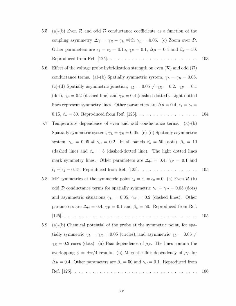
5.5 (a)-(b) Even R and odd D conductance coefficients as a function of the
coupling asymmetry ∆γ = γR − γL with γL = 0.05. (c) Zoom over D.
Other parameters are ǫ1 = ǫ2 = 0.15, γP = 0.1, ∆µ = 0.4 and βa = 50.
Reproduced from Ref. [125]. . . . . . . . . . . . . . . . . . . . . . . . . . 103
5.6 Effect of the voltage probe hybridization strength on even (R) and odd (D)
conductance terms. (a)-(b) Spatially symmetric system, γL = γR = 0.05.
(c)-(d) Spatially asymmetric junction, γL = 0.05 6= γR = 0.2. γP = 0.1
(dot), γP = 0.2 (dashed line) and γP = 0.4 (dashed-dotted). Light dotted
lines represent symmetry lines. Other parameters are ∆µ = 0.4, ǫ1 = ǫ2 =
0.15, βa = 50. Reproduced from Ref. [125]. . . . . . . . . . . . . . . . . . 104
5.7 Temperature dependence of even and odd conductance terms. (a)-(b)
Spatially symmetric system, γL = γR = 0.05. (c)-(d) Spatially asymmetric
system, γL = 0.05 6= γR = 0.2. In all panels βa = 50 (dots), βa = 10
(dashed line) and βa = 5 (dashed-dotted line). The light dotted lines
mark symmetry lines. Other parameters are ∆µ = 0.4, γP = 0.1 and
ǫ1 = ǫ2 = 0.15. Reproduced from Ref. [125]. . . . . . . . . . . . . . . . . 105
5.8 MF symmetries at the symmetric point ǫd = ǫ1 = ǫ2 = 0. (a) Even R (b)
odd D conductance terms for spatially symmetric γL = γR = 0.05 (dots)
and asymmetric situations γL = 0.05, γR = 0.2 (dashed lines). Other
parameters are ∆µ = 0.4, γP = 0.1 and βa = 50. Reproduced from Ref.
[125]. . . . . . . . . . . . . . . . . . . . . . . . . . . . . . . . . . . . . . . 105
5.9 (a)-(b) Chemical potential of the probe at the symmetric point, for spa-
tially symmetric γL = γR = 0.05 (circles), and asymmetric γL = 0.05 6=
γR = 0.2 cases (dots). (a) Bias dependence of µP . The lines contain the
overlapping φ = ±π/4 results. (b) Magnetic flux dependency of µP for
∆µ = 0.4. Other parameters are βa = 50 and γP = 0.1. Reproduced from
Ref. [125]. . . . . . . . . . . . . . . . . . . . . . . . . . . . . . . . . . . . 106
xv
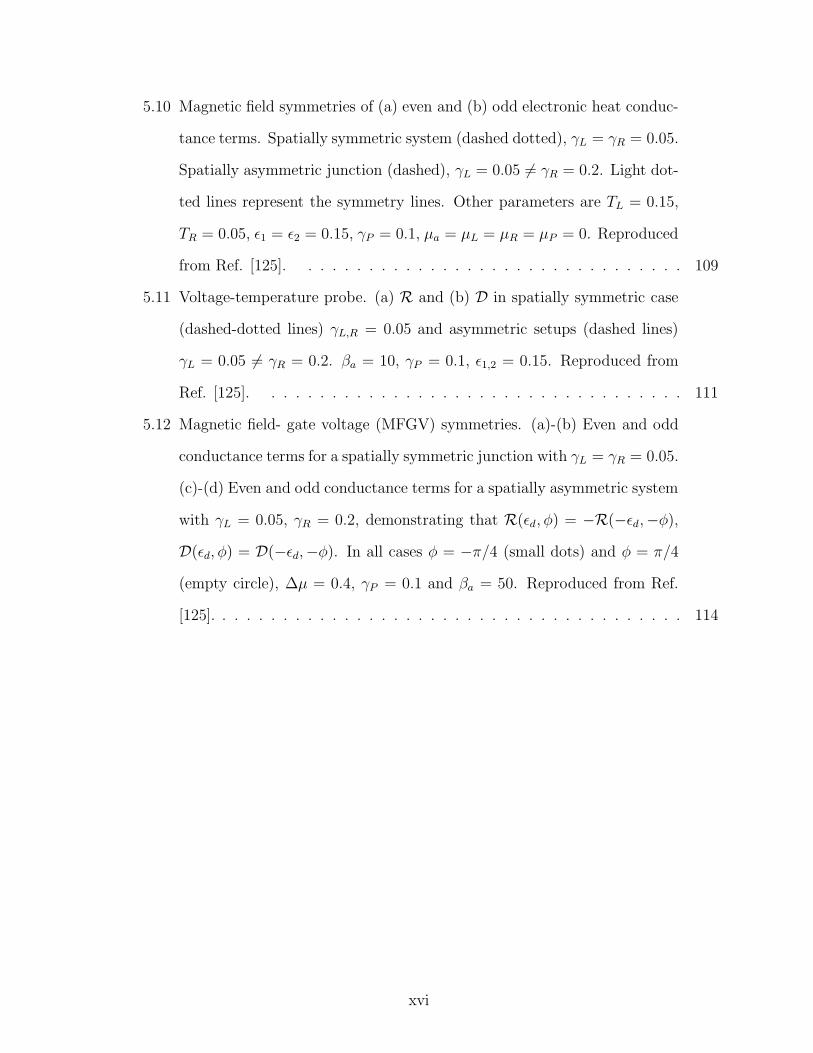
5.10 Magnetic field symmetries of (a) even and (b) odd electronic heat conduc-
tance terms. Spatially symmetric system (dashed dotted), γL = γR = 0.05.
Spatially asymmetric junction (dashed), γL = 0.05 6= γR = 0.2. Light dot-
ted lines represent the symmetry lines. Other parameters are TL = 0.15,
TR = 0.05, ǫ1 = ǫ2 = 0.15, γP = 0.1, µa = µL = µR = µP = 0. Reproduced
from Ref. [125]. . . . . . . . . . . . . . . . . . . . . . . . . . . . . . . . 109
5.11 Voltage-temperature probe. (a) R and (b) D in spatially symmetric case
(dashed-dotted lines) γL,R = 0.05 and asymmetric setups (dashed lines)
γL = 0.05 6= γR = 0.2. βa = 10, γP = 0.1, ǫ1,2 = 0.15. Reproduced from
Ref. [125]. . . . . . . . . . . . . . . . . . . . . . . . . . . . . . . . . . . 111
5.12 Magnetic field- gate voltage (MFGV) symmetries. (a)-(b) Even and odd
conductance terms for a spatially symmetric junction with γL = γR = 0.05.
(c)-(d) Even and odd conductance terms for a spatially asymmetric system
with γL = 0.05, γR = 0.2, demonstrating that R(ǫd, φ) = −R(−ǫd,−φ),
D(ǫd, φ) = D(−ǫd,−φ). In all cases φ = −π/4 (small dots) and φ = π/4
(empty circle), ∆µ = 0.4, γP = 0.1 and βa = 50. Reproduced from Ref.
[125]. . . . . . . . . . . . . . . . . . . . . . . . . . . . . . . . . . . . . . . 114
xvi
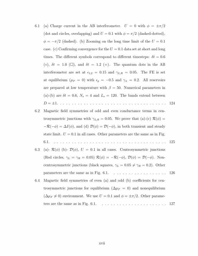
6.1 (a) Charge current in the AB interferometer. U = 0 with φ = ±π/2
(dot and circles, overlapping) and U = 0.1 with φ = π/2 (dashed-dotted),
φ = −π/2 (dashed). (b) Zooming on the long time limit of the U = 0.1
case. (c) Confirming convergence for the U = 0.1 data set at short and long
times. The different symbols correspond to different timesteps: δt = 0.6
(◦), δt = 1.0 (�), and δt = 1.2 (+). The quantum dots in the AB
interferometer are set at ǫ1,2 = 0.15 and γL,R = 0.05. The FE is set
at equilibrium (µF = 0) with ǫp = −0.5 and γ± = 0.2. All reservoirs
are prepared at low temperature with β = 50. Numerical parameters in
(a)-(b) are δt = 0.6, Ns = 4 and Ls = 120. The bands extend between
D = ±1. . . . . . . . . . . . . . . . . . . . . . . . . . . . . . . . . . . . . 124
6.2 Magnetic field symmetries of odd and even conductance terms in cen-
trosymmetric junctions with γL,R = 0.05. We prove that (a)-(c) R(φ) =
−R(−φ) = ∆I(φ), and (d) D(φ) = D(−φ), in both transient and steady
state limit. U = 0.1 in all cases. Other parameters are the same as in Fig.
6.1. . . . . . . . . . . . . . . . . . . . . . . . . . . . . . . . . . . . . . . 125
6.3 (a)- R(φ) (b)- D(φ), U = 0.1 in all cases. Centrosymmetric junctions
(Red circles, γL = γR = 0.05) R(φ) = −R(−φ), D(φ) = D(−φ). Non-
centrosymmetric junctions (black squares, γL = 0.05 6= γR = 0.2). Other
parameters are the same as in Fig. 6.1. . . . . . . . . . . . . . . . . . . 126
6.4 Magnetic field symmetries of even (a) and odd (b) coefficients for cen-
trosymmetric junctions for equilibrium (∆µF = 0) and nonequilibrium
(∆µF 6= 0) environment. We use U = 0.1 and φ = ±π/2. Other parame-
ters are the same as in Fig. 6.1. . . . . . . . . . . . . . . . . . . . . . . 127
xvii

List of symbols
A Vector potential
B Magnitude of magnetic field
Φ0 Flux quantum, Φ0 = h/e
Φ Magnetic flux
φ Aharonov-Bohm phase factor, φ = 2πΦΦ0
ǫ1 Energy of dot “1”
ǫ2 Energy of dot “2”
U Strength of electron-electron repulsion. In model I it stands for interdot electron
electron repulsion, in model III it stands for capacitive coupling to a fermionic
environment
Ed Shifted dot energy. It is defined as Ed = ǫ1(2) +U2
ξβ,l Tunneling element of dot 1(2) to the left reservoir
ζβ,r Tunneling of element of dot 1(2) to the right reservoir
D Cutoff energy of electronic bands
fν(ω) Fermi-Dirac distribution function for the νth reservoir, where ν = L,R and ω is
energy of bath electrons
xviii
µν Chemical potential of the νth reservoir
Tν Temperature of the νth reservoir
ρ Total density matrix, page 17
σ Reduced density matrix of the double-dot system, page 17
I Symmetrized charge current operator, page 68
Nν Number operator for ν reservoir
Iν Average current at the νth reservoir, page 17
Qν Average heat current at the νth reservoir, page 17
G+(ω) Retarded Green’s function, page 20
G−(ω) Advanced Green’s function, page 20
Tν,ν′(ω) Transmission probability from ν to ν ′ reservoir, page 21
Σν±(ω) Retarded (advanced) self energy contribution from νth reservoir
ΓL Hybridization matrix to the left reservoir, page 45
ΓR Hybridization matrix to the right reservoir, page 45
ΓP Hybridization matrix to the probe reservoir, page 60
xix
γL(R) Hybridization strengths to left/right reservoirs, γL = 2π∑
l ξβ,lδ(ω− ωl)ξ∗β′,l, γR =
2π∑
r ζβ,rδ(ω − ωr)ζ∗β′,r, see page 44
γp Hybridization to the probe reservoir, defined similary as above, page 60
Γ Total diagonal decay defined as Γ = γL + γR, page 67
γ± Magnetic flux dependent decay rates, page 48
fp(ω) Distribution function in the dephasing probe, page 25
µa Averaged chemical potential, µa =µL+µR
2
Ta Average temperature, Ta =TL+TR
2
∆µ Voltage bias, ∆µ = µL − µR
∆T Temperature bias, ∆T = TL − TR
δn Dots’ occupation difference
δt Time step in numerical path integral simulations
Ns Number of time slices in path integral simulations
τc Correlation time in path integral simulations, τc = Nsδt
xx
Chapter 1
Introduction
1.1 Aharonov-Bohm effect
The Aharonov-Bohm effect is a quantum mechanical phenomenon in which a charged
particle is affected by an electromagnetic field, despite being confined in a region where
electric and magnetic fields are zero [1]. This is because even if the magnetic field is
zero, the vector potential A affects the phase of the particle wavefunction. This can be
illustrated from the interference effect: Consider the schematic setup in Fig. 1.1, where
S is an electron source, the bold arrows show two paths, and a uniform magnetic field of
magnitude B is introduced perpendicular to the plane of the interferometer. This field
may be produced by an infinitely long thin cylinder. The vector potential A(r) is then
given by,
A(r) =
Brφ2
: r < R,
BR2φ2r
: r > R,
where B is the magnitude of magnetic field, φ is a unit vector along the z axis, R is the
radius of the cylinder and r is the radial coordinate. An electron passing through the
lower arm will follow the direction of the vector potential, and the one in the upper arm
1
Chapter 1. Introduction 2
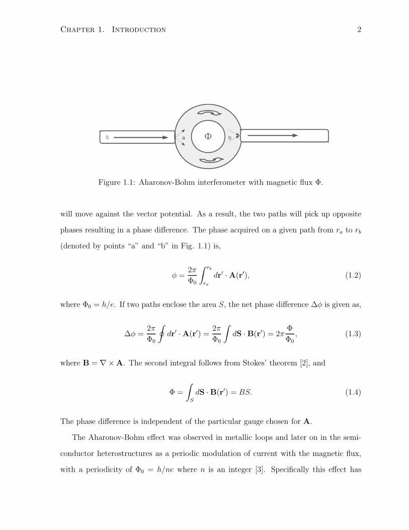
Figure 1.1: Aharonov-Bohm interferometer with magnetic flux Φ.
will move against the vector potential. As a result, the two paths will pick up opposite
phases resulting in a phase difference. The phase acquired on a given path from ra to rb
(denoted by points “a” and “b” in Fig. 1.1) is,
φ =2π
Φ0
∫ rb
ra
dr′ ·A(r′), (1.2)
where Φ0 = h/e. If two paths enclose the area S, the net phase difference ∆φ is given as,
∆φ =2π
Φ0
∮
dr′ ·A(r′) =2π
Φ0
∫
dS ·B(r′) = 2πΦ
Φ0, (1.3)
where B = ∇×A. The second integral follows from Stokes’ theorem [2], and
Φ =
∫
S
dS ·B(r′) = BS. (1.4)
The phase difference is independent of the particular gauge chosen for A.
The Aharonov-Bohm effect was observed in metallic loops and later on in the semi-
conductor heterostructures as a periodic modulation of current with the magnetic flux,
with a periodicity of Φ0 = h/ne where n is an integer [3]. Specifically this effect has
Chapter 1. Introduction 3
Figure 1.2: Scheme of a parallel double-dot Aharonov-Bohm interferometer. The mag-netic flux is denoted by Φ. The lines represent two electron paths between the source (S)and drain (D) electrodes.
been demonstrated in mesoscopic rings, with a single quantum dot structure integrated
into one of the arms in a ring, and in double-dot structures [4, 5]. These experiments,
and others, demonstrated that charge transport in these mesoscopic systems is phase
coherent.
In Fig 1.2 we include a scheme of coherently coupled parallel double-dot Aharonov-
Bohm interferometer realized by Holleitner et al. [5]. The device included a two-
dimensional electron gas below the surface of an AlGaAs/GaAs heterostructure. Schottky
gates were built by using electron beam writing and gold evaporation. These gates form
two quantum dots subjected to voltage bias applied through source (S) - drain (D) ter-
minals. The magnetic field was applied in a direction perpendicular to the device and
Aharonov-Bohm oscillations of the conductance were demonstrated.
1.2 Motivation
Aharonov-Bohm devices offer tunable systems, a natural laboratory to study the interplay
of quantum interference and many body effects in solid state environments. Experimental
and theoretical studies of such devices will be useful for understanding decoherence,
Chapter 1. Introduction 4
dissipation and transport in open quantum systems. In this work we use the double-
dot AB interferometer as a case study, to explore fundamental problems such as the
effect of electron-electron interactions on coherence dynamics, and transport far-from-
equilibrium. In the next subsections we outline some general problems, motivating this
work. In chapter 2 we present specific open questions, addressed in this thesis.
1.2.1 Coherent transport, many body interactions and deco-
herence
Is electron transfer through quantum dot structures phase coherent, or incoherent? How
do electron-electron and electron-phonon interactions affect phase-coherent transport?
From the other direction, what is the role of the interference phenomena on many body
effects, such as the formation of the Kondo resonance? These questions were addressed
in numerous experimental and theoretical works, detecting the presence of quantum co-
herence in mesoscale and nanoscale objects, using Aharonov-Bohm (AB) interferometry,
see for example Refs. [4, 5, 6, 7, 8, 9, 10, 11, 12, 13, 14, 15, 16, 17, 18, 19].
In particular, oscillations in the conductance resonances of an AB interferometer, with
either one or two quantum dots embedded in its arms, were experimentally demonstrated
in Refs. [4, 5], indicating the presence of quantum coherence. Interestingly, AB oscilla-
tions were also manifested in the co-tunneling regime, implying that phase coherence is
involved within such processes [14]. More recently, quantum transport through a paral-
lel configuration of two coherently coupled silicon dopants forming an Aharonov-Bohm
interferometer has been experimentally studied [20] demonstrating that the Kondo effect
can be coherently modulated by changing the magnetic flux. This device was also shown
to exhibit phase coherent transport in the sequential tunneling regime.
The steady state properties of the quantum dot Aharonov-Bohm (AB) interferometer
have been intensively investigated [6, 21], with the motivation to explore coherence effects
in electron transmission within mesoscopic and nanoscale structures [4, 7]. Particularly,
Chapter 1. Introduction 5
the role of electron-electron (e-e) interactions in AB interferometry has been considered
in Refs. [8, 9, 10, 11, 12, 22, 23], revealing, e.g., asymmetric interference patterns [8]
and the enhancement [12] or elimination [24] of the Kondo physics. Recent works further
considered the possibility of magnetic-field control in molecular transport junctions [13,
19, 25, 26].
Considering the role of electron-electron interactions in AB interferometry, a system-
atic theoretical analysis carried out in Ref. [8] has argued that electron-electron repulsion
effects, resulting in spin flipping channels for transferred electrons, induce dephasing. The
consequence of this decohering effect was the suppression of AB oscillations and the ap-
pearance of an asymmetry in the resonance peaks. One should note however that this
study has assumed infinitely strong e-e interactions and treated the system perturba-
tively in the dot-metals coupling strength. In other studies, e-e repulsion effects were
ignored [27], incorporated using a mean-field scheme, see for example [15], or treated
perturbatively using the Green’s function formalism [28, 29]. These studies, and other
theoretical and numerical works [8, 25], have typically considered only the steady state
limit, analyzing the conductance, a linear response quantity, or the current behavior,
often in the infinite large bias case [9, 10].
The double-quantum dot Aharonov-Bohm interferometer provides an important real-
ization of a qubit, where interference effects can be controlled by magnetic flux. Entangled
states of electrons are also of interest in solid state quantum computing. The quantum
dot setup can be used to design spin and charge qubits. As we have discussed in Sec
1.1, such a scheme can be realized by tunnel-coupled quantum dots, each of which con-
tains one single (excess) electron whose spin or charge state defines the qubit. Probing
the entanglement of electrons in a double-dot AB interferometer via transport noise was
suggested by Loss et al. [30].
The above studies mainly focused on steady state properties of quantum dot AB
interferometers. The real-time dynamics of these systems has been of recent interest,
Chapter 1. Introduction 6
motivated by the challenge to understand quantum dynamics, particularly decoherence
and dissipation, in open nonequilibrium many body systems. Studies of electron dynam-
ics in double-dot AB interferometers in the absence of e-e interactions have been carried
out in Refs. [31, 32, 33], using a non-markovian master equation approach. The detailed
non-perturbative analysis of transient dynamics of coherences and charge current for an
interacting case was carried out in our work, Ref. [34].
The coherence of electron transfer processes through an AB interferometer has been
typically identified and characterized via conductance oscillations in magnetic fields.
However, in a double-dot AB structure, a device including two dots, both connected
to biased metal leads, it is imperative that the relative phase between the two dot states
(or charge states) should similarly convey information on electron coherence and deco-
herence.
In my thesis I focus on several different models of a double-dot Aharonov-Bohm
interferometer, and demonstrate nontrivial magnetic flux dependent effects, arising from
the interplay of nonequilibrium effects, quantum coherence and many body interactions.
The dynamics of the interacting case is presented in Sec. 4.3 using numerically exact
influence functional path integral technique (INFPI) and quantum master equations.
1.2.2 Nonlinear magneto-transport
The theory of linear irreversible thermodynamics provides relations between thermody-
namic fluxes and thermodynamic forces,
J = LX. (1.5)
Here J is a column vector denoting the heat and particle current fluxes, X denotes a
column vector of thermodynamic forces related to the temperature and voltage bias, and
L is the Onsager matrix. Its diagonal elements are conductances, and the off-diagonal
Chapter 1. Introduction 7
elements are related to the Seebeck and Peltier coefficients [35, 36, 37].
Onsager-Casimir symmetry: Time reversal symmetry dictates reciprocal relations
between linear response coefficients, Li,j = Lj,i. In the presence of a magnetic field B the
reciprocity relation becomes
Li,j(B) = Lj,i(−B). (1.6)
From the above equation we can immediately see that the conductances (diagonal matrix
elements) are even functions of the magnetic field. In a two-terminal Aharonov-Bohm
interferometer this symmetry is known as the “phase rigidity” of linear conductance [4].
In the non-linear regime, Onsager-Casimir symmtries need not hold. A prominent
example of this breakdown is the asymmetry of the differential conductance out-of-
equilibrium [38, 39, 40, 41, 42]. This effect has been attributed to electron-electron
interactions in the system, resulting in an asymmetric charge response under the reversal
of a magnetic field, leading to a magnetoasymmetric differential conductance. Such an
interaction induced asymmetry has been observed recently in carbon nanotubes and also
in semiconductor quantum dots [38]. It is also of interest to investigate whether the
Onsager-Casimir symmetry can be fully or partially restored beyond linear response, in
the presence of many body interactions.
It is reasonable to argue that many body interactions may induce different types of
phase breaking processes in a coherent transport. These include, quasi-elastic scattering
and inelastic scattering. Buttiker’s probes are phenomenological tools to incorporate
quasi-elastic and inelastic scattering effects. Our objective is to study systematically
how many body effects and spatial asymmetries affect magnetic field symmetries and
magnetoasymmetries of charge and heat current beyond linear response. The detailed
discussion of different types of probes is presented in sec. 2.2.3.
Nonlinear transport measurement: Nonlinear transport measurements have been per-
formed recently on Aharonov-Bohm rings connected to two leads by Leturcq et al. [39],
reporting that the even (odd) conductance terms [coefficients of even and odd bias pow-
Chapter 1. Introduction 8
ers, see Eq. (2.46)] are asymmetric (symmetric) in magnetic field. It was also argued that
these observations were insensitive to geometric asymmetries in the ring. Angers et al.
[40] have also performed nonlinear transport measurements on GaAs/GaAlAs rings in a
two-terminal configuration, reporting an antisymmetric (under the reversal of magnetic
field) second order response coefficient, and attributed to e-e interactions. It should be
noted that in Ref. [39] no particular symmetry of even coefficients was reported, but
in Ref. [40] it was reported to be antisymmetric (under reversal of magnetic field). It
is essential to understand these scenarios theoretically. In this work we analytically ob-
tain conditions for an antisymmetric and asymmetric even coefficients, using Buttiker’s
probes, Sec. 5.4.
Interaction with an external nonequilibrium environment: Magnetic field asymmetries
of transport in mesoscopic conductors coupled to an environment have been theoretically
studied by Kang et al. [41]. The model system used in Ref. [41] was a quantum dot
conductor coupled to another conductor (treated as an environment) via a Coulomb in-
teraction. This allowes energy exchange between the conductor and the environment,
without particle exchange. The environment was then driven out-of-equilibrium by ap-
plying a voltage bias. It was found that the interaction between the conductor and the
environment causes magnetoasymmetry even in the linear regime, if the environment is
maintained out-of-equilibrium.
Motivated by this study, we explore magnetoasymmetries of transport when a double
quantum dot interferometer is coupled capacitively to an external fermionic environment.
While in early studies, the capacitive interaction was either treated at the mean-field level
or perturbatively [41, 43], we aim for numerically exact results. We unfold symmetry
relations by calculating the current in a double-dot setup, using a numerically exact
influence functional path integral method, see Sec. 2.2.4 for details. These results can be
used to benchmark and validate certain perturbative non-equilibrium Green’s function
schemes. Interestingly, we find that Buttiker probes obey the same symmetry relations
Chapter 1. Introduction 9
as those reached in a microscopic model.
1.2.3 Thermoelectric transport
The thermoelectric effect describes the conversion of a temperature gradient into a volt-
age, and vice versa. Strong demand for cost effective energy, and at the same time,
environmentally friendly energy sources, are the driving forces for research activity in
this area. Enhancing the efficiency of thermoelectric materials is one of the main themes
of current research in thermoelectrics.
A general thermoelectric setup consists of a system in contact with two reservoirs,
left (L) and right (R) with different temperatures and chemical potentials. In the linear
response regime the performance of a bulk thermoelectric device is characterized by a
single dimensionless parameter known as the figure of merit ZT . This quantity is given
by a combination of transport coefficients, electrical conductivity σ, thermal conductivity
κ, thermopower S, and temperature T . In terms of these quantities the figure of merit
reads as, ZT = (σS2/κ)T . It can be shown that the efficiency is given by,
η = ηc
√ZT + 1− 1√ZT + 1 + 1
(1.7)
where ηc = 1 − Tc
THis the Carnot efficiency, reached in the limit ZT → ∞. The linear
response approximation may be justified for bulk systems since it is possible to have large
temperature difference across the sample and yet very small gradients in temperature. In
nanoscale systems temperature and electrical potential gradients develop on the nanome-
ter scale which may lead to nonlinear effects. One can still analyze the performance of
nanoscale devices using an expression analogous to Eq. (1.7), [36].
Thermodynamics does not impose any upper bound on ZT , but the inter-relation
between electric and thermal transport properties makes it extremely hard to increase
the value of ZT beyond 1. It was recently argued that by breaking time reversal symmetry
Chapter 1. Introduction 10
one may enhance thermoelectric performance [36]. This is because in broken time reversal
symmetric systems the efficiency depends on (i) the magnetic field asymmetry of the
thermopower and (ii) on the figure of merit. Thus, to enhance efficiency, it is important
to understand how many body interactions and phase breaking processes affect transport
in nanoscale systems in the nonlinear regime [36].
1.2.4 Diode behaviour in Aharonov-Bohm interferometers
Diodes are integral components in electronic circuits. The diode effect can be realized by
combining many body interactions and spatial asymmetries. As an example, a theoretical
model of a thermal diode using a 1-dimensional lattice exploiting anharmonicity in the
form of onsite interactions and spatial asymmetry has been proposed in Refs. [44, 45, 46].
Thermal diodes were also experimentally realized in carbon and boron nitride nanotubes
[46]. In this thesis, we investigate the diode effect in the AB interferometer; sufficient
conditions are obtained analytically. We begin with a general two-terminal model, and
then demonstrate our results numerically using a specific model of a double-dot AB
interferometer, Sec. 5.6.
Chapter 2
Double-dot Aharonov-Bohm
interferometer
2.1 Models
In this section we present several models of double-dot Aharonov-Bohm interferometers.
These different models include distinct many body effects. We construct separate models
for two reasons. First, it is technically difficult to solve the dynamics of a complex system,
involving different types of many body interactions (electron-electron, electron-phonon,
electron-magnetic impurities), and thus to simplify our modeling we construct several-
complementary models incorporating distinct effects. Second, from the fundamental
point of view, it is actually advantagenous to study simplified models which allow us to
isolate different many body effects.
In this work we principally focus on quantum transport through a double-dot Aharonov-
Bohm interferometer. In our modeling, we include only those levels in each dot that
participate in the transport process. For simplicity, we include only one level in each
dot. Also, we do not consider the spin degree of freedom and focus on the dynamics and
steady state characterstics of the dots’ occupation, coherences and the net charge cur-
11
Chapter 2. Double-dot Aharonov-Bohm interferometer 12
rent. The quantum dots are connected to two metallic leads by a tunneling junction. The
leads comprise noninteracting electrons in a thermodynamic equilibrium. The assump-
tion of noninteracting electrons follows from Landau-Fermi-liquid theory [47, 48, 49].
The key ideas behind this theory are the notion of adiabacity and the Pauli’s exclusion
principle. Consider a system of noninteracting electrons, and suppose we turn on the
electron-electron interaction slowly. According to Landau-Fermi arguments, the ground
state of Fermi-gas would adiabatically transform in to the ground state of the interacting
system. By Pauli’s exclusion principle, the ground state of Fermi gas consists of fermions
occupying all momentum states corresponding to momentum p < pf , where pf is the
fermi momentum. As we turn on the interaction, the spin, charge and momentum of
the fermions corresponding to occupied states remain unchanged, while the dynamical
properties such as their mass, magnetic moment etc. are renormalized to new values
[50]. Thus, there is a one-to-one corrospondence between the elementary excitations of a
Fermi gas and a Fermi liquid system. In the context of Fermi liquid systems, these excita-
tions are known as “quasi-particles”. This leads to a picture of effectively noninteracting
electrons. The Hamiltonian of this system has the following form,
HAB = HS +HB +HSB. (2.1)
Here HS comprises the isolated double-dot system, HB represents the metallic leads, and
HSB includes the tunneling element between the leads and the two dots. For simplicity,
we set ~ = 1, kB = 1, and electron charge e = 1 throughout this work.
2.1.1 Model I: Closed interferometer with Coulomb repulsion
In this model (spinless) electrons experience an inter-dot electron-electron (e-e) repulsion
of strength U , see Fig. 2.1
Chapter 2. Double-dot Aharonov-Bohm interferometer 13
!L
T
!R
T
"2
"1
Un1n2
Figure 2.1: Model I. The two dots are each represented by a single electronic level.Coulombic repulsion energy is represented by the double arrow. The total magnetic fluxis denoted by Φ.
In second quantization the Hamiltonian of the isolated double-dot system is given by
HS = ǫ1a†1a1 + ǫ2a
†2a2 + Ua†1a1a
†2a2, (2.2)
where ǫ1,2 are the energies of the single level dots. The third term Ua†1a1a†2a2 stands for
the (nontrivial) inter-dot Coulomb repulsion. To keep our discussion general, we allow
the states to be nondegenerate at this point. Here a†β and aβ are the subsystem creation
and annihilation operators, respectively, where β = 1, 2 denotes dots ’1’ and ’2’. The
metal leads are composed of noninteracting electrons,
HB =∑
l
ωla†lal +
∑
r
ωra†rar, (2.3)
where a†l,r and al,r are the creation and annihilation operators respectively, for an electron
of energy ωl,r in the left (l) or right (r) lead. The Fermi-Dirac distribution functions
fν(ω) = [eβν(ω−µν)+1]−1describes the electronic occupations of the leads, where µν , ν =
L,R is the chemical potential and we denote by βν = 1Tν
the inverse temperature for νth
reservoir. The subsystem-bath coupling term is given by
HSB =∑
β,l
ξβ,la†βale
iφLβ +
∑
β,r
ζβ,ra†raβe
iφRβ + h.c., (2.4)
where ξ is the tunneling element of dot electrons to the left bath, and similarly ζ stands
Chapter 2. Double-dot Aharonov-Bohm interferometer 14
for tunneling to the right bath. Here φLβ and φR
β are the AB phase factors, acquired by
electron waves in a magnetic field perpendicular to the device plane. These phases are
constrained to satisfy the following relation
φL1 − φL
2 + φR1 − φR
2 = φ = 2πΦ/Φ0, (2.5)
where Φ is the magnetic flux enclosed by the ring and Φ0 = hc/e is the flux quantum.
In what follows we adopt the gauge
φL1 − φL
2 = φR1 − φR
2 = φ/2. (2.6)
Throughout this thesis we use the same gauge; our results are independent of this par-
ticular choice.
We apply a voltage bias ∆µ ≡ µL − µR, with µL,R as the chemical potential of the
metals. While we bias the system in a symmetric manner, µL = −µR, the dot levels may
be placed away from the so called “symmetric point” at which µL − ǫβ = ǫβ − µR. This
situation may be achieved by applying a gate voltage to each dot.
2.1.2 Model II: Interferometer with probes; elastic and inelastic
effects
Our second model allows dephasing and inelastic effects of electrons in the interferometer
by using Buttiker’s probe technique, as explained in Sec. 2.2.3. The schematic setup of
this model is shown in Fig. 2.2. For simplicity, in this model we do not include explicit
electron-electron interactions, setting U = 0; the probe technique effectively introduces
many body effects, from different sources. We augment the Hamiltonian (2.1) with a
Chapter 2. Double-dot Aharonov-Bohm interferometer 15
ΦµL
T
µR
T
ε
ε
µP, T
dot 2
dot 1
Figure 2.2: Model II. The two dots are each represented by a single electronic level,which do not directly couple. The total magnetic flux is denoted by Φ. The electrons ofdot ’1’ may be susceptible to dephasing or inelastic effects, introduced here through thecoupling of this dot to a Buttiker’s probe, the terminal P . Different types of probes arepresented in Sec. 2.3
probe, adding to the system a noninteracting electron reservoir P ,
H = HAB +∑
p∈Pωpa
†pap +
∑
p∈Pλpa
†1ap + h.c. (2.7)
The parameter λp, assumed to be real, denotes the coupling strength of dot ’1’ to the
P terminal. The parameters of the probe terminal are determined self-consistently so
as to introduce elastic dephasing or inelastic scattering of electrons as we explain in
subsection 2.2.3. Note that we only allow here for local scattering events on dot ’1’. One
could similarly consider models in which both dots are susceptible to scattering effects,
possibly from different sources.
2.1.3 Model III: Interferometer capacitively coupled to a fermionic
environment
In our third model the double quantum dot interferometer is capacitively coupled to
a fermionic environment which may be driven out of equilibrium, see Fig. 2.3. The
Chapter 2. Double-dot Aharonov-Bohm interferometer 16
Hamiltonian for this model is given by
H = HAB +HF +Hint. (2.8)
The AB Hamiltonian is given by Eq. (2.1), but for simplicity we do not include the inter-
dot electron-electron interactions within the interferometer. The AB interferometer is
electrostatically interacting, without exchanging particles, with a fermionic environment
(FE), realized here by the junction,
HF = ǫpc†pcp +
∑
s∈±ǫsc
†scs +
∑
s∈±gsc
†scp + h.c. (2.9)
It includes a quantum dot of energy ǫp coupled to two reservoirs (s = ±). We distin-
guish between the AB interferometer and the FE by adopting the operators c† and c to
denote creation and annihilation operators of electrons in the FE. Electrons in the AB
interferometer and the FE compartment are interacting according to the form
Hint = Unpn1. (2.10)
Here np = c†pcp, n1 = a†1a1 are the number operators, and U is the charging energy,
reflecting repulsion effects when dot ’1’ in the AB interferometer and level p in the
fermionic environment are occupied. The FE may be set at equilibrium when µ+ = µ−
(with the Fermi energy set at zero), or biased away from equilibrium using ∆µF ≡
µ+ − µ− 6= 0. It introduces energy dissipation effects of electrons on dot 1, this system
provides a microscopic-physical description of the probe model II.
2.2 Observables and methods
In this thesis we focus on following observables:
Chapter 2. Double-dot Aharonov-Bohm interferometer 17
Figure 2.3: Model III. Scheme for a double-dot Aharonov Bohm interferometer coupledto a fermionic environment. This environment is made of a quantum dot (labeled p) itselfcoupled to either (a) an equilibrium sea of noninteracting electrons, or (b) two metals(±) possibly biased away from equilibrium. In both cases, the dissipative environmentis introduced through a capacitive interaction of dot ’1’ of the interferometer to the dotp in the environment.
1. The reduced density matrix: σβ,β′(t) = 〈a†β(t)aβ′(t)〉 = Tr[ρ(t)a†βaβ′ ], where β, β ′ =
1, 2 are indices for the dots, and ρ is the total density matrix.
2. The average charge current: The charge current at left contact is given by
IL = 〈IL(t)〉 = Tr[ρ(t)IL], (2.11)
where the current operator is defined as
IL = −dNL
dt= −i[H, NL] (2.12)
with the number operator NL ≡ ∑
l a†lal. Here H is the total Hamiltonian of a
given model. Similarly, we can write an expression for the current at the right lead.
In what follows we denote the averaged charge current by I.
Ongoing miniaturization of electronic devices down to the nanoscale has triggered the-
oretical and computational research aiming to describe coherent transport and nonequi-
librium many body effects. In perturbative analytic methods, such as the nonequilibrium
Green’s function technique, the typical perturbation parameter is U/Γ, where U is the
Chapter 2. Double-dot Aharonov-Bohm interferometer 18
strength of the Coulomb interaction and Γ is the coupling strength to the metallic leads.
Other semi-analytic approaches, based upon the renormalization group principles are the
time dependent density matrix renormalization group (TDMRG) technique, and func-
tional renormalization group (FRG) method. The key ingredient of TDMRG is the
representation of the total wavefunction in a truncated but optimized basis, instead of
working in the full Hilbert space [51]. The basic idea behind FRG is the formulation of
“flow equations” for the self energy accounting its full frequency dependence [52]. The
starting point of this method is the exact solution in the noninteracting limit. During
the flow, the self energy is continuously transformed, and the solution of the interact-
ing problem is achieved when the flow terminates. This method can be combined with
diagrammatic perturbation theory on the Keldysh contour.
As an alternative to the above methods, brute force numerical methods have been
developed for studying nonequilibrium quantum transport through nanostructures. The
real-time quantum Monte-Carlo (QMC) technique is well established [53], but compu-
tations are limited to short-intermediate simulation times because of the notorious sign
problem. A novel method based on the QMC technique with complex chemical potentials
has been recently developed in Ref. [54].
A different idea based on the deterministic iterative summation of path integrals
(ISPI) was developed in Ref. [55]. This method was developed for studying the dynamics
of the single impurity Anderson model, and its validity has been confirmed by a detailed
comparison to other methods. A related approach, known as the “influence functional
path integral” (INFPI) method is based on the deterministic iterative evaluation of the
influence functional [56, 57]. This approach has been applied to the spin-fermion model
and to other multi-level impurity models. It relies on the observation that in out-of-
equilibrium cases bath correlations have a finite range, allowing truncation of the influence
functional [56, 57].
Chapter 2. Double-dot Aharonov-Bohm interferometer 19
In this work, we study model I without an inter-dot Coulomb repulsion U using
the quantum Langevin equation approach, which is equivalent to the Green’s function
technique in the U = 0 limit. Furthermore, we employ an exact fermionic trace formula
for studying the transient dynamics of the noninteracting case. We then simulate the
interacting model using (INFPI) method. This is the first time that this system is studied
using a nonperturbative and deterministic technique. Model II is investigated using the
nonequilibrium Green’s function method along with Buttiker’s probes. The dynamics
of charge current in model III is studied using INFPI. In the next subsection we briefly
explain the methods used in this work.
2.2.1 Nonequilibrium Green’s function technique
The nonequilibrium Green’s function (NEGF) technique was rigrously developed by
Schwinger in a classic mathematical paper [58], treating the Brownian motion of a quan-
tum oscillator. The next important development in this field was due to Kadanoff and
Baym who derived quantum kinetic equations [59] . A diagrammatic expansion in pow-
ers of the coupling to the environment was developed by Keldysh with the key idea of
contour ordering [60]. These initial developments were done in the early 1960s. Another
important development in the context of quantum transport was an explicit derivation
of a formula for the transmission function in terms of the Green’s function, by Caroli et
al. [61].
In this work, we use the Green’s function method to obtain closed expressions for the
reduced density matrix and the charge current in the case of a noninteracting (U = 0)
double-dot AB interferometer. The treatment that we adopt is based on the quan-
tum Langevin equation (QLE) approach [62]. We note that in the noninteracting limit
(U = 0), quantum Langevin equation, nonequilibrium Green’s function technique, and
scattering approaches, are equivalent. A detailed derivation of the QLE method is pre-
sented in section 3.2, the main expressions are included below. The reduced density
Chapter 2. Double-dot Aharonov-Bohm interferometer 20
matrix for the double-dot (α, β = 1, 2) system in the noninteracting case reads [62],
〈a†αaβ〉 ≡ σα,β =1
2π
∫ ∞
−∞
[
(
G+ΓLG−)
α,βfL(ω) +
(
G+ΓRG−)
α,βfR(ω)
]
dω.(2.13)
Here the matrices G+ and G− = (G+)† are the retarded and advanced Green’s functions,
and fL(ω) and fR(ω) are the Fermi-Dirac distribution functions in the left and right
reservoirs. The matrix elements of G+ are given by
G+β,α(ω) =
1
(ω − ǫβ)δα,β − ΣL,+β,α (ω)− ΣR,+
β,α (ω). (2.14)
In the above equation ΣL,+β,α (ω) and ΣR,+
β,α (ω) are the self energies, see Eq. (3.6) for details.
In Eq. (2.13) ΓL(R) are the hybridization matrices to the left and right reservoirs, with
the matrix elements
ΓLβ,β′(ω) = 2πe
i(φLβ−φL
β′)∑
l
ξβ,lδ(ω − ωl)ξ∗β′,l, (2.15)
and
ΓRβ,β′(ω) = 2πe
−i(φRβ −φR
β′)∑
r
ζβ,rδ(ω − ωr)ζ∗β′,r. (2.16)
Eq. (2.13) can be extended to describe any number of reservoirs. When a probe reservoir
is included (discussed in the next section), it reads as below,
〈a†αaβ〉 =1
2π
∑
ν=L,R,P
∫ ∞
−∞
(
G+ΓνG−)
α,βfν(ω)dω. (2.17)
An expression for the charge current, in the case of noninteracting dots, is given below,
see Eq. (2.18).
Chapter 2. Double-dot Aharonov-Bohm interferometer 21
2.2.2 Landauer-Buttiker approach
In the scattering formalism of Landauer and Buttiker [63, 64, 65, 66], interactions between
particles are neglected. Considering a multi-terminal setup, one can express the charge
current from the ν to the ν ′ terminal in terms of the transmission probability Tν,ν′(ω), a
function which depends on the energy of the incident electron,
Iν(φ) =
∫ ∞
−∞dω[
∑
ν′ 6=ν
Tν,ν′(ω, φ)fν(ω)−∑
ν′ 6=ν
Tν′,ν(ω, φ)fν′(ω)]
. (2.18)
The Fermi-Dirac distribution function fν(ω) = [eβν(ω−µν )+1]−1 is defined in terms of the
chemical potential µν and the inverse temperature βν . The magnetic field is introduced
via an Aharonov-Bohm flux Φ applied perpendicular to the conductor, with the magnetic
phase φ = 2πΦ/Φ0. The transmission function can be written in terms of the Green’s
function of the system and the self energy matrices,
Tν,ν′ = Tr[ΓνG+Γν′G−]. (2.19)
Explicit expressions for a particular model are included in Sec. 5.5. We consider a setup
including three terminals, L, R and P , where the P terminal serves as the “probe”, see
Fig. 2.2. The probe properties are determined by self-consistent conditions discussed
in the next subsection. We focus below on the steady state charge current from the L
reservoir to the central system (IL), and from the probe to the system (IP ),
IL(φ) =
∫ ∞
−∞dω[
TL,R(ω, φ)fL(ω)− TR,L(ω, φ)fR(ω)
+ TL,P (ω, φ)fL(ω)− TP,L(ω, φ)fP (ω, φ)]
, (2.20)
Chapter 2. Double-dot Aharonov-Bohm interferometer 22
IP (φ) =
∫ ∞
−∞dω[
TP,L(ω, φ)fP (ω, φ)− TL,P (ω, φ)fL(ω)
+ TP,R(ω, φ)fP (ω, φ)− TR,P (ω, φ)fR(ω)]
. (2.21)
Similarly, we can write the heat current at the ν = L terminal as
QL(φ) =
∫ ∞
−∞dω (ω − µL)
[
TL,R(ω, φ)fL(ω)
−TR,L(ω, φ)fR(ω) + TL,P (ω, φ)fL(ω)− TP,L(ω, φ)fP (ω, φ)]
. (2.22)
The heat current at the probe is given by an analogous expression. The probe distri-
bution function is determined by the probe condition. It is generally influenced by the
magnetic flux, as we demonstrate in Eqs. (2.24)-(2.27). For convenience, we simplify
next our notation. First, we drop the reference to the energy of incoming electrons ω in
both transmission functions and distribution functions. Second, since the integrals are
evaluated between ±∞, we do not put the limits explicitly. Third, unless otherwise men-
tioned, fP , µP and all transmission coefficients are evaluated at the phase +φ, thus we
do not explicitly write the phase variable. If we do need to consider e.g. the transmission
function Tν,ν′(−φ), we write instead the complementary expression, Tν′,ν(φ).
2.2.3 Buttiker’s Probes technique
Phase-breaking and energy dissipation processes arise due to the interaction of electrons
with other degrees of freedom, e.g., with electrons, phonons, and defects. While an
understanding of such effects, from first principles, is the desired objective of numerous
computational approaches [67], simple analytical treatments are advantageous as they
allow one to gain insights into transport phenomenology.
The markovian quantum master equation and its variants (Lindblad, Redfield) is
simple to study and interpret [68], and as such it has been extensively adopted in studies
of charge, spin, exciton, and heat transport. It can be derived systematically, from
Chapter 2. Double-dot Aharonov-Bohm interferometer 23
projection operator techniques [69], and phenomenologically by introducing damping
terms into the matrix elements of the reduced density matrix, to include dephasing and
inelastic processes into the otherwise coherent dynamics.
Buttiker’s probe technique [66, 70, 71] and its modern extensions to thermoelectric
problems [72, 35, 36, 73], atomic-level thermometry [74], and beyond linear response
situations [75, 76, 77, 78, 79] present an alternative route for introducing decoherence
and inelastic processes into coherent conductors. The probe is an electronic component
[80], and it allows one to obtain information about local variables, chemical potential
and temperature, deep within the conductor. When coupled strongly to the system, the
probe can alter intrinsic transport mechanisms.
The probe technique can be exercised in several different ways, to induce distinct ef-
fects: Elastic dephasing processes are implemented by incorporating a “dephasing probe”,
enforcing the requirement that the net charge current towards the probe terminal, at any
given energy, vanishes [81, 82]. Inelastic heat dissipative effects are included by a “voltage
probe”, by demanding that the total-net charge current to the probe terminal nullifies
[66, 70, 71]. This process dissipates heat since electrons leaving the system to the probe
re-enter the conductor after being thermalized. In the complementary “temperature
probe” charge leakage is allowed at the probe, but the probe temperature is tuned such
that the net heat current at the probe is nil [84]. The “voltage-temperature probe”, also
referred to as a “thermometer”, requires both charge current and heat current at the
probe to vanish. In this case inelastic - energy exchange effects are allowed on the probe,
but heat dissipation and charge leakage effects are excluded.
The probe technique has been used in different applications, particularly for the ex-
ploration of the ballistic to diffusive (Ohm’s law and Fourier’s law) crossover in electronic
[70, 85] and phononic conductors [86, 87, 88, 89]. More recently, the effect of thermal
rectification has been studied in phononic systems by utilizing the temperature probe as
a mean to incorporate effective anharmonicity [75, 76, 77, 90]. A full-counting statistics
Chapter 2. Double-dot Aharonov-Bohm interferometer 24
analysis of conductors including dephasing and voltage probes has been carried out in
Ref. [91]. The probe parameters, temperature and chemical potential, can be derived
analytically when the conductor is set close to equilibrium [66, 80, 72]. Far from equilib-
rium, while these parameters can be technically defined and their uniqueness [78] allows
for a physical interpretation, an exact analytic solution is missing. However, recent stud-
ies have demonstrated that iterative numerical schemes can reach a stable solution for the
temperature probe [76, 79]. These techniques have been then used for following phononic
heat transfer in the deep quantum limit, far from equilibrium [76, 79].
Dephasing probe: Elastic dephasing effects can be incorporated with the dephasing
probe. A particle entering the probe is incoherently re-emitted within a small energy
interval [ω, ω+ dω] such that dω << Tν ,∆µ [92]. It loses phase memory, but the change
in energy is much smaller than the voltage bias and the temperature [92]. Since scattering
processes in each energy interval are independent, the distribution function of electrons
in the probe reservoir is a highly nonequilibrium one, see Eq. (2.24). Elastic dephasing
effects can thus be implemented by demanding that the energy-resolved particle current
vanishes in the probe,
IP (ω) = 0 with IP =
∫
IP (ω)dω. (2.23)
Using this condition, Eq. (2.21) provides a closed form for the corresponding (flux-
dependent) probe distribution, not necessarily in the form of a Fermi function,
fP (φ) =TL,PfL + TR,PfR
TP,L + TP,R. (2.24)
Voltage probe: Dissipative inelastic effects can be introduced into the conductor using
the voltage probe technique. The three reservoirs (L, R, P) are maintained at the same
inverse temperature βa, but the L and R chemical potentials are made distinct, µL 6= µR.
In this case the chemical potential µP of the probe P is evaluated by demanding that
Chapter 2. Double-dot Aharonov-Bohm interferometer 25
the net-total particle current flowing into the P reservoir diminishes,
IP = 0. (2.25)
This choice allows for dissipative energy exchange processes to take place within the
probe. In the linear response regime Eq. (2.21) can be used to derive an analytic
expression for µP ,
µP (φ) =∆µ
2
∫
dω ∂fa∂ω
(TL,P − TR,P )∫
dω ∂fa∂ω
(TP,L + TP,R). (2.26)
In the above equation the derivative of the Fermi function is evaluated at equilibrium. In
far-from-equilibrium situations we obtain the unique [78] chemical potential of the probe
numerically by using the Newton-Raphson method [161]
µ(k+1)P = µ
(k)P − IP (µ
(k)P )
[
∂IP (µ(k)P )
∂µP
]−1
. (2.27)
The current IP (µ(k)P ) and its derivative are evaluated from Eq. (2.21) using the probe
(Fermi) distribution with µ(k)P . Note that the self-consistent probe solution varies with
the magnetic flux.
Temperature probe: In this scenario the three reservoirs L,R,P are maintained at
the same chemical potential µa, but the temperature at the L and R terminals are made
different, TL 6= TR. The probe temperature TP = β−1P is determined by requiring the net
heat current at the probe to satisfy
QP = 0. (2.28)
This constraint allows for charge leakage into the probe since we do not require Eq.
(2.25) to hold. We can obtain the temperature TP numerically by following an iterative
Chapter 2. Double-dot Aharonov-Bohm interferometer 26
procedure,
T(k+1)P = T
(k)P −QP (T
(k)P )
[
∂QP (T(k)P )
∂TP
]−1
. (2.29)
The probe temperature varies with the applied flux φ.
Voltage-temperature probe: This probe acts as an electron thermometer at weak
coupling. This is achieved by setting the temperatures TL,R and the potentials µL,R, then
demand that both
IP = 0 , QP = 0. (2.30)
In other words, the charge and heat currents in the conductor satisfy IL = −IR and
QL = −QR, since neither charges nor heat are allowed to leak to the probe. Analytic
results can be obtained in the linear response regime, see for example Refs. [72, 85].
Beyond that, equation (2.30) can be solved self-consistently, to provide TP and µP . This
can be done by using the two-dimensional Newton-Raphson method,
µ(k+1)P = µ
(k)P −D−1
1,1IP (µ(k)P , T
(k)P )−D−1
1,2QP (µ(k)P , T
(k)P )
T(k+1)P = T
(k)P −D−1
2,1IP (µ(k)P , T
(k)P )−D−1
2,2QP (µ(k)P , T
(k)P ), (2.31)
where the Jacobean D is re-evaluated at every iteration,
D(µP , TP ) ≡
∂IP (µP ,TP )∂µP
∂IP (µP ,TP )∂TP
∂QP (µP ,TP )∂µP
∂QP (µP ,TP )∂TP
We emphasize that besides the case of the dephasing probe, the function fP (φ) is forced
to take the form of a Fermi-Dirac distribution function in the other probe models.
Chapter 2. Double-dot Aharonov-Bohm interferometer 27
2.2.4 Influence functional path integral simulations
This technique allows one to follow the nonequilibrium real-time dynamics of electrons
in a subsystem-bath model (for example, the double-dot-metals) by performing exact
numerical simulations [56, 57]. The principles of the INFPI approach have been detailed
in Refs. [56, 57], where it has been adopted for investigating dissipation effects in the
nonequilibrium spin-fermion model, and the population and the current dynamics in cor-
related quantum dots, by investigating the single impurity Anderson model [84] and the
two-level spinless Anderson dot [93, 94]. In this thesis, we further extend this approach,
examining the effect of a magnetic flux on the intrinsic coherence dynamics in Model-I.
We also use this tool and study symmetries of nonlinear transport in Model III.
The INFPI method relies on the observation that in out-of-equilibrium (and/or finite
temperature) cases bath correlations have a finite range, allowing for their truncation
beyond a memory time dictated by the voltage-bias and the temperature. Taking ad-
vantage of this fact, an iterative-deterministic time-evolution scheme has been developed
where convergence with respect to the memory time can in principle be reached [56, 57].
As convergence is facilitated at large bias, the method is well suited for the description
of the real-time dynamics of devices driven to a steady state via interaction with biased
leads. The INFPI approach is complementary to other numerically exact methods such as
numerical renormalization group techniques [95, 96], real time quantum Monte Carlo sim-
ulations [53] and path integral methods [55]. It offers flexibility in defining the impurity
subsystem and the metal band structure. The results converge well at intermediate-large
voltage bias and/or high temperatures as shown in section-4.3. We outline now the tech-
nical principles of the INFPI method as developed in references [56, 57]. We begin by
reorganizing the Hamiltonian, Eq. (2.1), as H = H0 + H1, identifying the nontrivial
quartic many body interaction term in model I, Eq. (2.2) as
H1 = U
[
n1n2 −1
2(n1 + n2)
]
. (2.32)
Chapter 2. Double-dot Aharonov-Bohm interferometer 28
In a similar manner, the quartic many body interaction term in model III, Eq. (2.10)
can be organized. H0 contains the remaining two-body terms, redefining the dot energies
as Ed,β = ǫβ + U/2. This partitioning allows us to utilize the Hubbard-Stratonovich
(HS) transformation [154], see Eq. (2.34) below. Formally, the dynamics of a quadratic
operator, A, either given in terms of the baths (metals) or impurity degrees of freedom,
can be written as
〈A(t)〉 = Tr[ρ(t0)A(t)] = limλ→0
∂
∂λTr[
ρ(0)eiHteλAe−iHt]
. (2.33)
Here λ is a real number, taken to vanish at the end of the calculation, ρ is the total density
matrix, and the trace is performed over both the subsystem and the reservoirs degrees of
freedom. For simplicity, we assume that at the initial time t = 0 the dots and the baths
are decoupled, ρ(0) = σ(0)⊗σL⊗σR. The baths are prepared in a nonequilibrium biased
state σν ; the subsystem is described by the (reduced) density matrix σ(0). We proceed
and factorize the time evolution operator, eiHt = (eiHδt)N , further utilizing the Trotter
decomposition eiHδt ≈(
eiH0δt/2eiH1δteiH0δt/2)
. The many body term H1 can be eliminated
by introducing auxiliary Ising variables s = ± via the HS transformation [154],
e±iH1δt =1
2
∑
s
eH±(s); eH±(s) ≡ e−sκ±(n2−n1). (2.34)
Here κ± = κ′∓iκ′′, κ′ = sinh−1[sin(δtU/2)]1/2, κ′′ = sin−1[sin(δtU/2)]1/2. The uniqueness
of this transformation requires Uδt < π. Incorporating the Trotter decomposition and
the HS transformation into Eq. (2.33), the time evolution of A is dictated by
〈A(t)〉 = limλ→0
∂
∂λ
{
∫
ds±1 ds±2 , ..., ds
±NI(s
±1 , s
±2 , ..., s
±N)}
. (2.35)
The integrand, referred to as an “Influence Functional” (IF), is given by (k = 1, k+ p =
Chapter 2. Double-dot Aharonov-Bohm interferometer 29
N),
I(s±k , ..., s±k+p) =
1
22(p+1)Tr[
σ(0)G+(s+k+p)...G+(s
+k )e
iH0(k−1)δteλAe−iH0(k−1)δtG−(s−k )...G−(s
−k+p)
]
(2.36)
Here G+(s+k ) =
(
eiH0δt/2eH+(s+k )eiH0δt/2)
and G− = G†+. Eq. (2.35) is exact in the
δt → 0 limit. Practically, it can be evaluated by noting that in standard nonequilibrium
situations, even at zero temperature, bath correlations die exponentially, thus the IF
in Eq. (2.35) can be truncated beyond a memory time τc = Nsδt, corresponding to
the time beyond which bath correlations may be controllably ignored [56]. Here Ns is
an integer and the correlation time τc is determined by the nonequilibrium situation,
roughly τc ∼ 1/∆µ. This argument implies the following (non-unique) breakup [56]
I(s±1 , s±2 , ...s
±N) ≃ I(s±1 , s
±2 , ..., s
±Ns)Is(s
±2 , s
±3 , ..., s
±Ns+1)...
×Is(s±N−Ns+1, s
±N−Ns+2, ..., s
±N), (2.37)
where each element in the product, besides the first one, is given by a ratio between
truncated IF,
Is(sk, sk+1, ..., sk+Ns−1) =I(s±k , s
±k+1, ..., s
±k+Ns−1)
I(s±k , s±k+1, ..., s
±k+Ns−2)
. (2.38)
It is useful to define the multi-time object and time-evolve it by multiplying it with the
subsequent truncated IF, over the intermediate variables,
R(s±k+1, s±k+2, ..., s
±k+Ns−1) =
∑
s±1 ,s±2 ,...,s±k
I(s±1 , s±2 , ..., s
±Ns)Is(s
±2 , s
±3 , ..., s
±Ns+1)....Is(s
±k , s
±k+1, ..., s
±k+Ns−1),
(2.39)
Chapter 2. Double-dot Aharonov-Bohm interferometer 30
then summing over the internal variables,
R(s±k+2, s±k+3, ..., s
±k+Ns
) =∑
s±k+1
R(s±k+1, s±k+2, ..., s
±k+Ns−1)Is(s
±k+1, s
±k+2, ..., s
±k+Ns
). (2.40)
Summation over the internal variables results in the time local expectation value,
〈eλA(tk)〉 =∑
s±k+2−Ns,...,s±k
R(s±k+2−Ns, s±k+3−Ns
, ..., s±k ). (2.41)
This procedure should be repeated for several (small) values of λ. Taking the numerical
derivative with respect to λ, the expectation value 〈A(tk)〉 is retrieved. The main element
in this procedure, the truncated IF [Eq. (2.36)], is calculated using a fermionic trace
formula [119],
I = Tr[
eM1eM2 ...eMp(σL ⊗ σR ⊗ σ(0))]
= det{
[IL − fL]⊗ [IR − fR]⊗ [IS − fS] + em1em2 ...emp [fL ⊗ fR ⊗ fS]}
. (2.42)
Here, σν , the time-zero density matrix of the ν = L,R fermion bath and σ(0), the
subsystem initial density matrix, are assumed to follow an exponential form. Other
terms eM , with M a quadratic operator, represent further factors in Eq. (2.36). In the
determinant, m is a single-particle operator, corresponding to the quadratic operator
M =∑
i,j(m)i,jc†icj ; c†i (cj) are fermionic creation and annihilation operators, either
related to the system or the baths. The matrices Iν and IS are the identity matrices
for the ν space and for the subsystem, respectively. The determinant in Eq. (2.42) is
evaluated numerically by taking into account Ls electronic states for each metal. This
discretization implies a numerical error. However, we have found that with Ls ∼ 100
states we can reach convergence in the time interval of interest. Other sources of error,
elaborated and examined in Refs. [56, 57], are the Trotter error, originating from the
Chapter 2. Double-dot Aharonov-Bohm interferometer 31
approximate factorization of the total Hamiltonian into the non-commuting H0 (two-
body) and H1 (many body) terms, and the memory error, resulting from the truncation
of the IF. Convergence is verified by demonstrating that results are insensitive to the
time step and the memory size, once the proper memory time is accounted for. It was
shown in Ref. [34] that when the dot states are located within the bias window a shorter
memory time is required for reaching convergence, in comparison to the case where the
dot energies are out-of-resonance with the bias window. This could be rationalized by
noting that the decorrelation time for electrons within the bias window is short relative
to the characteristic timescale of decay for electrons occupying off-resonance states.
It was also noted that distinct observables may require different memory time τc for
reaching convergence [34, 56, 57]. The dot’s occupation and the real part of the subsystem
off-diagonal element, ℜσ1,2, converge for τc ∼ 1/∆µ. In contrast, the charge current and
ℑσ1,2 require a memory time at least twice longer, as these quantities are sensitive to
the bias drop at each contact, rather than to the overall voltage bias. It is important to
note that this scaling is approximate, and the actual memory time further depends on
the subsystem (dots) energetics in a complex way. The memory time depends on U in
a nontrivial manner [97], and the position of the dot with respect to the left and right
chemical potentials also affects the convergence behavior.
In the absence of U , INFPI numerical results are exact, irrespective of the memory
size used in the simulation. This can be seen from Eqs. (2.36) and (2.37), where a
cancellation effect takes place leaving only free propagation terms, from t = 0 to the
current time. At infinitely large U one expects again superior convergence behavior, as
simultaneous occupancy is forbidden [97]. Since INFPI can not treat the infinite U case
in its current form, we adopted a particular quantum master equation to study this limit.
Chapter 2. Double-dot Aharonov-Bohm interferometer 32
2.2.5 Master equations at U = 0 and U = ∞
Several different types of quantum master equations have been developed to study quan-
tum transport through open systems and nanostructures [69, 98]. Given the vast lit-
erature in this field, we do not aim in reviewing it here. We only mention a specific
approach of interest, the Bloch-type rate equations based on the microscopic many body
Schrodinger equation as developed by Gurvitz [9]. In this thesis, we adopt master equa-
tions to complement our simulations with INFPI. The approach can be used in two
different limits, (i) U = 0, and (ii) U = ∞. The main assumptions in deriving these
equations are:
1. The system is subjected to a very large voltage bias, implying a unidirectional
transport.
2. The reservoirs have a broad band with energy independent density of states.
3. The reservoirs are Markovian; electron relaxation in the metals is fast compared to
electron dynamics in the junction.
We denote the reduced density matrix of the double-dot system in the charge state
basis as σj,j′(t), j = a, b, c, d. Here the index j labels the double-dot charge states in
order of an empty dot (a), single occupied dot, on either the ”1” or ”2” sites (b and c
states, respectively) and the state (d), with the two dots occupied. Explicitly, |a〉 ↔ |00〉,
|b〉 ↔ |10〉, |c〉 ↔ |01〉, and |d〉 ↔ |11〉. The creation and annihilation operators of the
dot are related to this states by a†1 ↔ |00〉〈01|+ |01〉〈11| and a†2 ↔ |00〉〈10| + |10〉〈11|.
Since a†1a2 ↔ |01〉〈01|, we identify the observable of interest σ1,2=Tr[σa†1a2] by σb,c. In
Chapter 2. Double-dot Aharonov-Bohm interferometer 33
the noninteracting (U = 0) case, the following equations hold in the infinite bias limit [9]
σa,a = −4γLσa,a + γR(
σb,b + σc,c + σb,ceiφ/2 + σc,be
−iφ/2)
σb,b = 2γLσa,a − 2(γR + γL)σb,b + 2γRσd,d + δγ∗eiφ/2σb,c + δγe−iφ/2σc,b
σc,c = 2γLσa,a − 2(γR + γL)σc,c + 2γRσd,d + δγ∗eiφ/2σb,c + δγe−iφ/2σc,b
σd,d = 2γL(
σb,b + σc,c − e−iφ/2σb,c − eiφ/2σc,b
)
− 4γRσd,d
σb,c = 2γLeiφ/2σa,a + δγ(σb,b + σc,c)e
−iφ/2 − 2γRσd,de−iφ/2 − 2(γL + γR)σb,c (2.43)
Here δγ = (eiφγL − γR). The hybridization strength, independent of the site index β, is
defined as γL = 2π∑
l ξ2l,βδ(ω − ωl), and γR = 2π
∑
l ζ2r,βδ(ω − ωr). The equations are
valid in the infinite bias limit, when |µL − µR| ≫ γL(R). The total probability, to occupy
any of the four states, is unity,∑
j=a,b,c,d σj,j = 1.
In the infinite U regime one can again derive the system’s equations of motion in
the large bias limit while excluding simultaneous occupancy at both dots, σd,d = 0. The
following equations of motion are then achieved [9, 99] (σa,a + σb,b + σc,c = 1),
σa,a = −4γLσa,a + 2γR(σb,b + σc,c + σb,ceiφ/2 + σc,be
−iφ/2)
σb,b = 2γLσa,a − 2γRσb,b − γR(σb,ceiφ/2 + σc,be
−iφ/2)
σc,c = 2γLσa,a − 2γRσc,c − γR(σb,ceiφ/2 + σc,be
−iφ/2)
σb,c = 2γLeiφ/2σa,a − γRe
−iφ/2(σb,b + σc,c)− 2γRσb,c. (2.44)
In chapter 4 we use master equations to study coherence dynamics in the U = 0 and
U = ∞ limits. We extract magnetic flux dependent decay rates, and study the long time
behaviour.
Chapter 2. Double-dot Aharonov-Bohm interferometer 34
2.3 Open questions
2.3.1 Quantum dynamics in nonequilibrium many body sys-
tems
The double quantum dot Aharonov-Bohm interferometer offers a rich playground for
studying fundamental questions of decoherence, dissipation and transport in open quan-
tum systems. This system has been intensively investigated in the context of Kondo
physics, Coulomb blockade behaviour, transmission phase lapses, coherent population
trapping [6, 4, 7, 8, 9, 10, 11, 12, 13, 5, 14, 15, 16, 17, 100, 101]. From the statistical
mechanics perspective, quantum dot interferometers have been used to verify quantum
fluctuation theorems and derive the counting statistics in broken time reversal symmet-
ric set-ups [91, 102]. However, the transient dynamics of this system has been mostly
ignored, partially because of the lack of appropriate methodologies. The magnetic flux
dependent dynamics is of a fundamental interest from the quantum information perspec-
tive. This aspect will be studied in this work. In order to achieve our objective, we will
utilize the modeling tools discussed in the previous section, and address the following
general questions:
1. What are the signatures of many body effects in the transient dynamics and the
steady state behaviour?
2. How does a finite bias voltage affect quantum coherent transport?
3. Are there symmetries which are obeyed in the steady state limit, but are violated
in the transient regime?
4. Can we understand the basic physics of transport using phenomenological models
of many body interactions?
Chapter 2. Double-dot Aharonov-Bohm interferometer 35
2.3.2 Transient dynamics and steady state behaviour (model I)
The behaviour of the charge current and dot occupations in nanodevices has been in-
tensively studied in the steady state limit using markovian master equations [31]. The
dynamics of coherences, the off-diagonal elements of the reduced density matrix, is of
particular interest from the quantum computing perspective. This coherence dynam-
ics was only recently studied by Tu et al. [31] who had investigated the dynamics of
a noninteracting double-dot interferometer using non-markovian master equations. It
was found that when the double-dot system is set at the particle-hole symmetric point
(µL − ǫ = ǫ− µR), and when φ 6= 2πp where p is an integer, the real part of coherence,
ℜ(σ1,2) = 0 and the imaginary part ℑ(σ1,2) 6= 0. In other words, the relative phase
between the two dot states (charge states) defined as
σ12(t) = |σ12|eiϕ(t) (2.45)
approaches ϕ = ±π/2 in the long-time limit. It was thus argued in Ref. [31] that one can
not manipulate this relative phase by changing the Aharonov-Bohm phase. This effect
has been refered as the “phase localization”. Since dot energies can be tuned away from
the particle-hole symmetric point by the gate voltage, it is of interest to explore if the
“phase localization” effect still holds away from the symmetric point.
The noninteracting system has further revealed a wealth of intricate behavior, such as
“flux-dependent level attraction” [27], and the ability to achieve decoherence control when
junction asymmetry is incorporated [33]. In this thesis we study transient and steady
state properties of the double quantum dot Aharonov-Bohm interferometer: population,
coherence and current. First, we consider the noninteracting case (U = 0) and unfold
novel transport characterstics induced by the interplay of magnetic flux, gate voltage,
and applied bias voltage. We obtain exact analytical expressions in the steady state
limit, and use an exact fermionic trace formula for the transient case, and address the

Chapter 2. Double-dot Aharonov-Bohm interferometer 36
following questions:
1. What is the effect of the gate voltage and voltage bias on the dynamics of coher-
ences, particularly away from the symmetric point?
2. How does the occupation of the dots change with the magnetic flux?
3. How does the temperature affect the occupation-flux behaviour?
4. What is the role of dephasing on the coherence behaviour?
We then focus on the dynamics of Model I with interactions (U 6= 0) and address the
following questions:
1. What is the role of finite electron-electron repulsion effects in the “phase localiza-
tion” effect, and how does it affect the charge current?
2. How does the system dynamics change in the U = ∞ limit, compared to the U = 0
case?
2.3.3 Magnetic field symmetries beyond linear response (model
II)
The Onsager-Casimir symmetry relations [37] are satisfied in phase-coherent conductors,
reflecting the microreversibility of the scattering matrix. For simplicity, consider a two-
terminal (L,R) quantum-dot Aharonov-Bohm interferometer. The net current I can be
written as,
I(φ,∆µ) = G1(φ)∆µ+G2(φ)∆µ2 + .... (2.46)
where G1(φ) is the linear conductance term and further terms are the non-linear conduc-
tances. According to the Onsager-Casimir symmetry relations, the linear conductance
should be an even function of magnetic field. In Aharonov-Bohm interferometers with
Chapter 2. Double-dot Aharonov-Bohm interferometer 37
conserved electron current this symmetry is displayed by the “phase rigidity” of the
(linear) conductance oscillations with the magnetic field B, G1(B) = G1(−B) [4, 21].
Beyond linear response, the phase symmetry of the conductance is not enforced, and
several experiments [38, 39, 40, 106, 103, 104, 105, 107, 108, 109] have demonstrated its
breakdown.
Supporting theoretical works have elucidated the role of many body interactions in the
system [10, 110, 111, 112, 113, 114], typically approaching the problem by calculating the
electrostatic screening potential within the conductor in a self-consistent manner, a pro-
cedure often limited to low-order conduction terms [10, 110, 112]. Magnetoasymmetries
in the closed single quantum dot interferometer with strong electron-electron interactions
have been analyzed beyond mean field theory by Lim et al. [107], demonstrating that in
a spatially symmetric system even conductance terms are odd in the magnetic flux, and
odd terms are even [107].
Although, the above studies focused on a particular realization of an Aharonov-Bohm
interferometer with specific a form of many body interactions, a model independent proof
of symmetry relations was missing. We show that such a proof can be constructed using
Buttiker’s probe technique, as the probes offer a phenomenological means to introduce
many body interactions. Our objective is to resolve the role of different scattering ef-
fects on transport symmetries beyond linear response. Specifically we focus on following
questions:
1. How does pure elastic dephasing affect the Onsager symmetry?
2. What is the role of inelastic scattering processes on transport symmetries beyond
linear response? Are there new symmetries beyond linear response?
3. What is the role of spatial symmetry and particle-hole symmetry on transport
symmetries?
4. Can the interferometer act as a diode when the time reversal symmetry is broken,
Chapter 2. Double-dot Aharonov-Bohm interferometer 38
though the device is geometrically symmetric?
2.3.4 Interferometer capacitively coupled to a fermionic envi-
ronment: transient dynamics and steady state (model III)
Considering model III representing a double-dot interferometer coupled capacitively to a
fermionic environment which may be out of equilibrium, see Fig. 2.3, we are interested
in the transient and steady state characterstics of this model, to extract magnetic field
symmetry relations. This model resembles a voltage probe in the sense that there is no
charge leakage from double-dot interferometer, but energy exchange between the double-
dot and the fermionic environment can occur. We particularly focus on the following
questions:
1. What is the role of fermionic environment in breaking the Onsager symmetry within
the AB interferometer beyond linear response?
2. Does the microscopic Hamiltonian model III support transport results as predicted
by a phenomenological tool, the voltage probe?
2.3.5 Thesis organization
This thesis is centered around applying the methods discussed in sec. 2.2 to understand
the various transport phenomena in models I, II and III. In chapter 3 we present the
derivation of the nonequilibrium Green’s function technique using the quantum Langevin
approach for model I at U = 0. We obtain closed expressions for the reduced density ma-
trix of the double-dot system and expose non-trivial magnetic flux-dependent effects. We
also analytically prove that in degenerate and symmetric interferometers, flux-dependent
occupation difference develops. The transient dynamics of the noninteracting model I is
studied using an exact fermionic trace formula.
Chapter 2. Double-dot Aharonov-Bohm interferometer 39
We complement this study and consider model II, a noninteracting double-dot in-
terferometer with a local dephasing probe. Using the nonequilibrium Green’s function
method and the dephasing probe condition, we compute the occupations of the dots an-
alytically and expose several nontrivial flux dependent effects away from the symmetric
point. While at the symmetric point dot occupations are independent of magnetic flux,
away from the symmetric point flux strongly affects the dots’ occupation. We further
demonstrate that when the dots’ energies are aligned with the chemcial potentials of
leads, new coherent oscillatory patterns develop and sustain, as long as the dephasing
strength is of the order of the applied voltage bias.
In chapter 4 we focus on the transient dynamics of model I with electron-electron re-
pulsion. Coherences and the charge current are simulated using INFPI. We show that the
temporal characterstics of coherences are preserved under weak-intermediate Coulomb in-
teraction strengths. We complement our study by using Bloch-type master equations in
two different limits, U = 0, and U = ∞. We show that the “phase localization” effect
does not hold in the U = ∞ limit. We also study the temperature dependence of the
coherences and the charge current. Some general observations about time scales are
discussed, and a detailed convergence analysis of INFPI is presented.
In chapter 5 we continue with model II and study the role of phase breaking pro-
cesses on the symmetries of nonlinear transport using Buttiker’s probe. We show that
under quasi-elastic dephasing processes Onsager symmetry is maintained beyond linear
response, and that there is no rectification of current. We then consider the role of in-
elastic scattering processes using the voltage probe technique. In this case, in the linear
response regime the Onsager symmetry is maintained but beyond that we show that, it
is broken. We analytically prove that for spatially symmetric systems odd conductance
terms are even in magnetic flux and even conductance terms are odd. We further demon-
strate that these symmetries are invalidated once spatial symmetry is broken, though at
the particle-hole symmetric point these symmetries do hold irrespective of spatial asym-
Chapter 2. Double-dot Aharonov-Bohm interferometer 40
metries. These observations hold for a general interferometer and we demonstrate these
results using the double-dot interferometer, model II. We show that the system can act
as a charge current rectifier when two conditions are met simultaneously: (i) many body
effects are included in the form of inelastic scattering; and (ii) time reversal symmetry
is broken. We then extend this discussion and study model II with the temperature
and voltage-temperature probes. We also obtain generalized magnetic field gate voltage
symmetries.
In chapter 6 we study Model III, a double-dot Aharonov-Bohm interferometer ca-
pacitively coupled to a fermionic environment. We perform simulations using INFPI
and show that the magnetic flux symmetries of odd-even conductance coefficients ob-
tained using the voltage probe, do hold for a capacitive coupling to an equilibrium or a
nonequilibrium environment. In chapter 7 we conclude and discuss future directions.
Chapter 3
Model I: Noninteracting electrons
3.1 Introduction
In this chapter, we focus on a simple-minimal model, the noninteracting double quantum
dot AB interferometer, and study its transient and steady state properties in biased
situations. We focus on a symmetric AB setup, with a quantum dot located at each arm
of the interferometer. The dots are connected to two metal leads (referred to as baths, or
reservoirs) maintained in a biased state. For a scheme of this model, see Fig. 2.1. Here
we consider the U = 0 case. In Sec. 3.2 we present the quantum Langevin approach
and obtain the reduced density matrix in terms of the retarded and advanced Green’s
functions. In Sec. 3.3 we obtain the steady state behaviour of the dots’ occupations,
coherences and current, and study the role of a gate voltage, magnetic flux, and bias.
In Sec. 3.4 we study the transient dynamics using the fermionic trace formula. Results
presented here were published in Ref. [115].
3.2 Equations of motion
The steady state characteristics of the noninteracting model can be calculated exactly
using the nonequilibrium Green’s function (NEGF) approach [116]. This technique has
41
Chapter 3. Model I: Noninteracting electrons 42
been extensively used in the past for studying transport properties in mesoscopic systems
and molecular junctions [117]. The derivation presented here follows an equation-of-
motion approach [62]. In this method, the quantum Langevin equation for the subsystem
is obtained by solving the Heisenberg equations of motion (EOM) for the baths’ variables,
then substituting them back into the EOM for the subsystem (dots) variables. The indices
α, β = 1, 2 identify the two dots. The resulting EOM for the operators of the subsystem
are [115]
daβdt
= −iǫβaβ − iηLβ − iηRβ
− i
∫ t
t0
dτ∑
α,l
ξβ,lg+l (t− τ) ξ∗α,le
i(φLβ−φL
α)aα(τ)
− i
∫ t
t0
dτ∑
α,r
ζ∗β,rg+r (t− τ) ζα,re
i(φRα−φR
β )aα(τ). (3.1)
The (isolated) reservoirs Green’s functions are given by
g+l (t) = −ie−iωltθ(t), g+r (t) = −ie−iωrtθ(t). (3.2)
In the language of the quantum Langevin approach, the terms ηLβ and ηRβ are referred to
as noise, induced on the subsystem from the left and right reservoirs, respectively. Here
ηLβ = i∑
l
ξβ,lg+l (t− t0) al(t0)e
iφLβ
ηRβ = i∑
r
ζ∗β,rg+r (t− t0) ar(t0)e
−iφRβ . (3.3)
As an initial condition we take a factorized state, ρ(t0) = σL ⊗ σR ⊗ σS(t0), with empty
dots and the reservoirs prepared in a grand canonical state, σν = e−(Hν−µνN)/Tν
Tr[e−(Hν−µνN)/Tν ], Tν
is the temperature of the ν = L,R fermi sea and µν stands for its chemical potential.
The reduced density matrix σS denotes the state of the subsystem. Using this initial
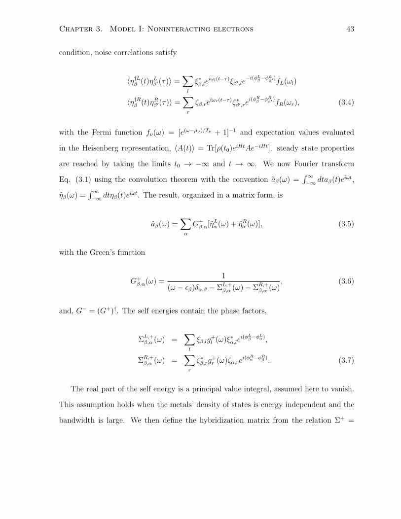
Chapter 3. Model I: Noninteracting electrons 43
condition, noise correlations satisfy
〈η†Lβ (t)ηLβ′(τ)〉 =∑
l
ξ∗β,leiωl(t−τ)ξβ′,le
−i(φLβ−φL
β′)fL(ωl)
〈η†Rβ (t)ηRβ′(τ)〉 =∑
r
ζβ,reiωr(t−τ)ζ∗β′,re
i(φRβ −φR
β′)fR(ωr), (3.4)
with the Fermi function fν(ω) = [e(ω−µν )/Tν + 1]−1 and expectation values evaluated
in the Heisenberg representation, 〈A(t)〉 = Tr[ρ(t0)eiHtAe−iHt]. steady state properties
are reached by taking the limits t0 → −∞ and t → ∞. We now Fourier transform
Eq. (3.1) using the convolution theorem with the convention aβ(ω) =∫∞−∞ dtaβ(t)e
iωt,
ηβ(ω) =∫∞−∞ dtηβ(t)e
iωt. The result, organized in a matrix form, is
aβ(ω) =∑
α
G+β,α[η
Lα(ω) + ηRα (ω)], (3.5)
with the Green’s function
G+β,α(ω) =
1
(ω − ǫβ)δα,β − ΣL,+β,α (ω)− ΣR,+
β,α (ω), (3.6)
and, G− = (G+)†. The self energies contain the phase factors,
ΣL,+β,α (ω) =
∑
l
ξβ,lg+l (ω)ξ
∗α,le
i(φLβ−φL
α),
ΣR,+β,α (ω) =
∑
r
ζ∗β,rg+r (ω)ζα,re
i(φRα−φR
β ). (3.7)
The real part of the self energy is a principal value integral, assumed here to vanish.
This assumption holds when the metals’ density of states is energy independent and the
bandwidth is large. We then define the hybridization matrix from the relation Σ+ =
Chapter 3. Model I: Noninteracting electrons 44
−iγ/2,
ΓLβ,β′(ω) = 2πe
i(φLβ−φL
β′)∑
l
ξβ,lδ(ω − ωl)ξ∗β′,l. (3.8)
Similar expressions hold for the R side. Using the steady state solution (3.5), we can
write down an expression for the reduced density matrix. Back-transformed to the time
domain it takes the form
〈a†αaβ〉 ≡ σα,β =1
2π
∫ ∞
−∞
[
(
G+ΓLG−)
α,βfL(ω) +
(
G+ΓRG−)
α,βfR(ω)
]
dω. (3.9)
The time variable has been suppressed since the result is only valid in the steady state
limit. We take ξβ,l and ζβ,r as real constants, independent of the level index and the
reservoir state, resulting in
ΓLβ,β′ = γLe
i(φLβ−φL
β′), ΓRβ,β′ = γRe
−i(φRβ −φR
β′), (3.10)
where
γL = 2π∑
l
ξβ,lδ(ω − ωl)ξ∗β′,l, γR = 2π
∑
r
ζβ,rδ(ω − ωr)ζ∗β′,r. (3.11)
Using these definitions, the matrix G+ takes the form
G+ =
ω − ǫ1 +i(γL+γR)
2iγL2eiφ/2 + iγR
2e−iφ/2
iγL2e−iφ/2 + iγR
2eiφ/2 ω − ǫ2 +
i(γL+γR)2
−1
(3.12)
and the hybridization matrices are given by
ΓL = γL
1 eiφ/2
e−iφ/2 1
, ΓR = γR
1 e−iφ/2
eiφ/2 1
(3.13)
Chapter 3. Model I: Noninteracting electrons 45
We can now calculate, numerically or analytically, the behavior of the reduced density
matrix under different conditions [32]. Since in this chapter we are only concerned with
symmetric dot-lead couplings, we take γL = γR = γ/2. Furthermore, we impose energy
degeneracy, ǫ1 = ǫ2 = ǫ. This choice simplifies the relevant matrices to
G+ =
ω − ǫ+ iγ2
iγ2cos φ
2
iγ2cos φ
2ω − ǫ+ iγ
2
−1
,
ΓL =γ
2
1 eiφ/2
e−iφ/2 1
, ΓR =
γ
2
1 e−iφ/2
eiφ/2 1
(3.14)
We present closed analytic expressions for the diagonal and off-diagonal elements of the
reduced density matrix in Sec. 3.3 Complementing numerical data for the real-time
dynamics are included in Sec. 3.4.
3.3 Stationary behaviour
3.3.1 Dots’ occupation and occupation difference
We discuss here two effects that persist away from the “symmetric point”, defined as
µL − ǫ = ǫ− µR: The occupations of the dots significantly vary with flux, and moreover,
the degenerate dots acquire different occupations. After presenting general expressions
away from the symmetric point, we consider other relevant cases: the finite-bias limit at
the symmetric point, the limit of infinite bias (which effectively reduces to the symmetric
point), and the case of φ = 2πn, n = 0, 1, 2...
Analytic results are obtained from Eqs. (3.9) and (3.14), recall that γL = γR = γ/2
and ǫ = ǫ1 = ǫ2. Organizing these expressions, we find that the occupation of dot ’1’,
Chapter 3. Model I: Noninteracting electrons 46
σ1,1 ≡ 〈a†1a1〉, is given by two integrals,
σ1,1 =γ
4π
∫ ∞
−∞fL(ω)dω
(ω − ǫ)2 + ω20 − 2ω0(ω − ǫ) cos φ
2
[(ω − ǫ)2 − ω20]
2+ [γ(ω − ǫ)]2
+γ
4π
∫ ∞
−∞fR(ω)dω
(ω − ǫ)2 + ω20 + 2ω0(ω − ǫ) cos φ
2
[(ω − ǫ)2 − ω20]
2+ [γ(ω − ǫ)]2
, (3.15)
where we have introduced the short notation
ω0 ≡γ
2sin
φ
2. (3.16)
Similarly, the occupation of level ’2’, σ2,2 ≡ 〈a†2a2〉, is given by
σ2,2 =γ
4π
∫ ∞
−∞fL(ω)dω
(ω − ǫ)2 + ω20 + 2ω0(ω − ǫ) cos φ
2
[(ω − ǫ)2 − ω20]
2+ [γ(ω − ǫ)]2
+γ
4π
∫ ∞
−∞fR(ω)dω
(ω − ǫ)2 + ω20 − 2ω0(ω − ǫ) cos φ
2
[(ω − ǫ)2 − ω20]
2+ [γ(ω − ǫ)]2
. (3.17)
In what follows we consider the zero temperature limit. The Fermi functions take then
the shape of step functions and the upper limits of the integrals are replaced by the
corresponding chemical potentials. We now study the contribution of the odd term in
the integrand. This term is responsible for the development of occupation difference
between the dots,
δn = σ1,1 − σ2,2 = − γ
4π
∫ µL
µR
dω4ω0(ω − ǫ) cos φ
2
[(ω − ǫ)2 − ω20]
2+ [γ(ω − ǫ)]2
(3.18)
We evaluate this using an integral of the form below,
I =
∫ c
d
x
(x2 − a2)2 + b2x2dx =
tan−1[
2a2−b2−2d2
b√4a2−b2
]
− tan−1[
2a2−b2−2c2
b√4a2−b2
]
b√4a2 − b2
(3.19)
where d = (µR−ǫ), c = (µL−ǫ), b = γ and a = γ2sin φ
2, leading to b
√4a2 − b2 = ±iγ2 cos φ
2
Chapter 3. Model I: Noninteracting electrons 47
and
2a2 − b2 − 2d2 = γ2
[
1
2sin2 φ
2− 1
]
− 2(µR − ǫ)2
2a2 − b2 − 2c2 = γ2
[
1
2sin2 φ
2− 1
]
− 2(µL − ǫ)2
We now reorganize Eq. (3.19) using the relations tan−1 x+ tan−1 y = tan−1(
x+y1−xy
)
and
tan−1 z = i2[ln(1− iz) − ln(1 + iz)], to find
I =ln[
F+(φ)F−(φ)
]
2γ2 cos φ2
, (3.20)
where we define
F±(φ) =γ4
8sin4 φ
2
−(µL − ǫ)2[γ2
2sin2 φ
2− (µR − ǫ)2 − γ2
(
1± cosφ
2
)
]
−(µR − ǫ)2[
γ2
2sin2 φ
2− (µL − ǫ)2 − γ2
(
1∓ cosφ
2
)]
.
(3.21)
We can also reorganize these factors as a sum of real quadratic terms,
F±(φ) =γ4
8sin4 φ
2+ 2(µL − ǫ)2(µR − ǫ)2
+γ2
2
(
cosφ
2± 1
)2
(µL − ǫ)2 +γ2
2
(
cosφ
2∓ 1
)2
(µR − ǫ)2. (3.22)
Attaching the missing prefactors, δn = − γ4π4ω0 cos
φ2I, we simplify Eq. (3.18) to
δn = −sin φ2
4πln
[
F+(φ)
F−(φ)
]
. (3.23)
Inspecting Eq. (3.23), we note that it vanishes in four different cases: (i) at zero bias,
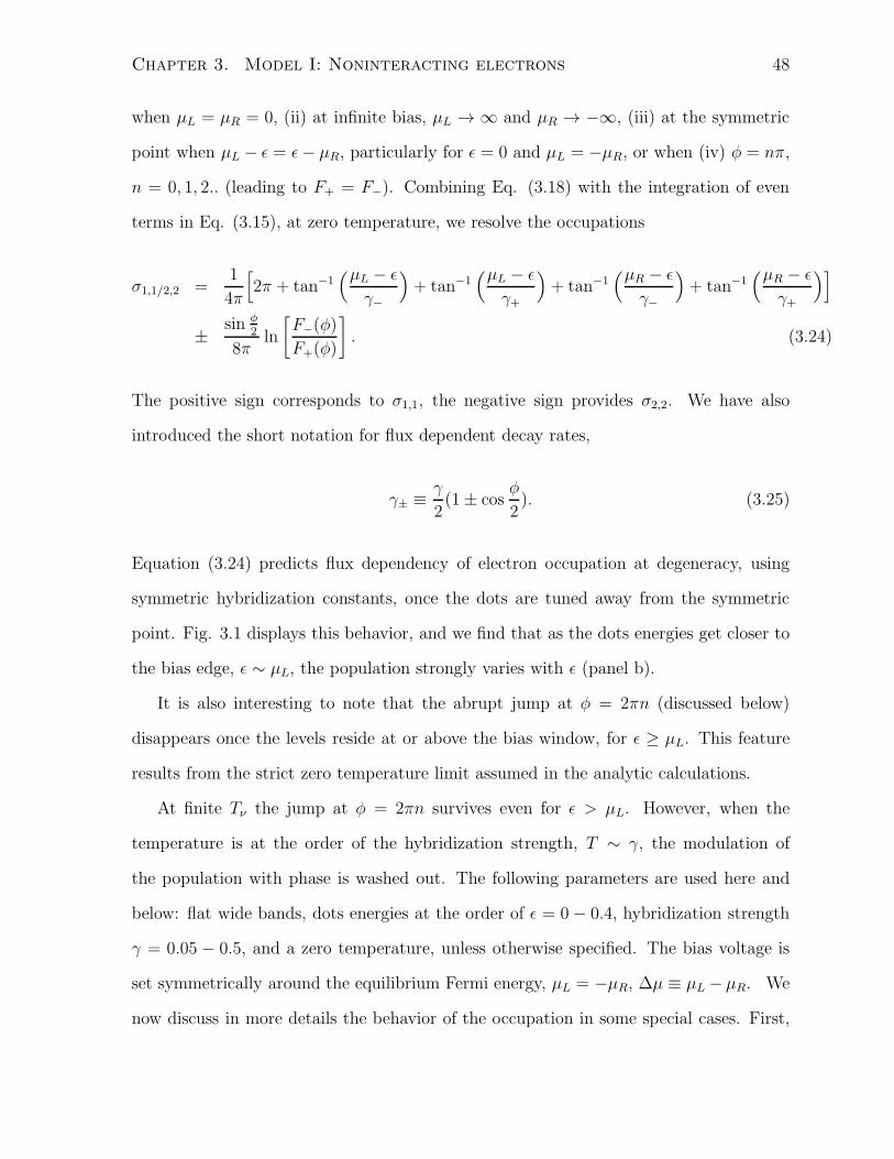
Chapter 3. Model I: Noninteracting electrons 48
when µL = µR = 0, (ii) at infinite bias, µL → ∞ and µR → −∞, (iii) at the symmetric
point when µL − ǫ = ǫ− µR, particularly for ǫ = 0 and µL = −µR, or when (iv) φ = nπ,
n = 0, 1, 2.. (leading to F+ = F−). Combining Eq. (3.18) with the integration of even
terms in Eq. (3.15), at zero temperature, we resolve the occupations
σ1,1/2,2 =1
4π
[
2π + tan−1(µL − ǫ
γ−
)
+ tan−1(µL − ǫ
γ+
)
+ tan−1(µR − ǫ
γ−
)
+ tan−1(µR − ǫ
γ+
)]
± sin φ2
8πln
[
F−(φ)
F+(φ)
]
. (3.24)
The positive sign corresponds to σ1,1, the negative sign provides σ2,2. We have also
introduced the short notation for flux dependent decay rates,
γ± ≡ γ
2(1± cos
φ
2). (3.25)
Equation (3.24) predicts flux dependency of electron occupation at degeneracy, using
symmetric hybridization constants, once the dots are tuned away from the symmetric
point. Fig. 3.1 displays this behavior, and we find that as the dots energies get closer to
the bias edge, ǫ ∼ µL, the population strongly varies with ǫ (panel b).
It is also interesting to note that the abrupt jump at φ = 2πn (discussed below)
disappears once the levels reside at or above the bias window, for ǫ ≥ µL. This feature
results from the strict zero temperature limit assumed in the analytic calculations.
At finite Tν the jump at φ = 2πn survives even for ǫ > µL. However, when the
temperature is at the order of the hybridization strength, T ∼ γ, the modulation of
the population with phase is washed out. The following parameters are used here and
below: flat wide bands, dots energies at the order of ǫ = 0− 0.4, hybridization strength
γ = 0.05 − 0.5, and a zero temperature, unless otherwise specified. The bias voltage is
set symmetrically around the equilibrium Fermi energy, µL = −µR, ∆µ ≡ µL − µR. We
now discuss in more details the behavior of the occupation in some special cases. First,
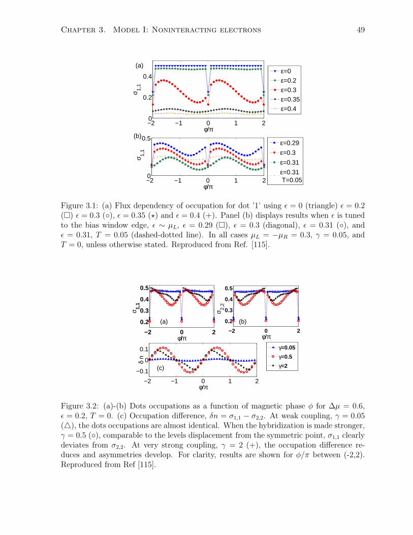
Chapter 3. Model I: Noninteracting electrons 49
−2 −1 0 1 20
0.2
0.4
φ/πσ 1,
1
(a)
(b)
ε=0
ε=0.2
ε=0.3
ε=0.35
ε=0.4
−2 −1 0 1 20
0.5
φ/π
σ 1,1
ε=0.29
ε=0.3
ε=0.31
ε=0.31 T=0.05
Figure 3.1: (a) Flux dependency of occupation for dot ’1’ using ǫ = 0 (triangle) ǫ = 0.2(�) ǫ = 0.3 (◦), ǫ = 0.35 (⋆) and ǫ = 0.4 (+). Panel (b) displays results when ǫ is tunedto the bias window edge, ǫ ∼ µL, ǫ = 0.29 (�), ǫ = 0.3 (diagonal), ǫ = 0.31 (◦), andǫ = 0.31, T = 0.05 (dashed-dotted line). In all cases µL = −µR = 0.3, γ = 0.05, andT = 0, unless otherwise stated. Reproduced from Ref. [115].
−2 0 2
0.2
0.3
0.4
0.5
σ 1,1
φ/π
(a)
−2 0 2
0.2
0.3
0.4
0.5
φ/π
σ 2,2
(b)
−2 −1 0 1 2
−0.1
0
0.1
φ/π
δ n
(c)
γ=0.05
γ=0.5
γ=2
Figure 3.2: (a)-(b) Dots occupations as a function of magnetic phase φ for ∆µ = 0.6,ǫ = 0.2, T = 0. (c) Occupation difference, δn = σ1,1 − σ2,2. At weak coupling, γ = 0.05(△), the dots occupations are almost identical. When the hybridization is made stronger,γ = 0.5 (◦), comparable to the levels displacement from the symmetric point, σ1,1 clearlydeviates from σ2,2. At very strong coupling, γ = 2 (+), the occupation difference re-duces and asymmetries develop. For clarity, results are shown for φ/π between (-2,2).Reproduced from Ref [115].
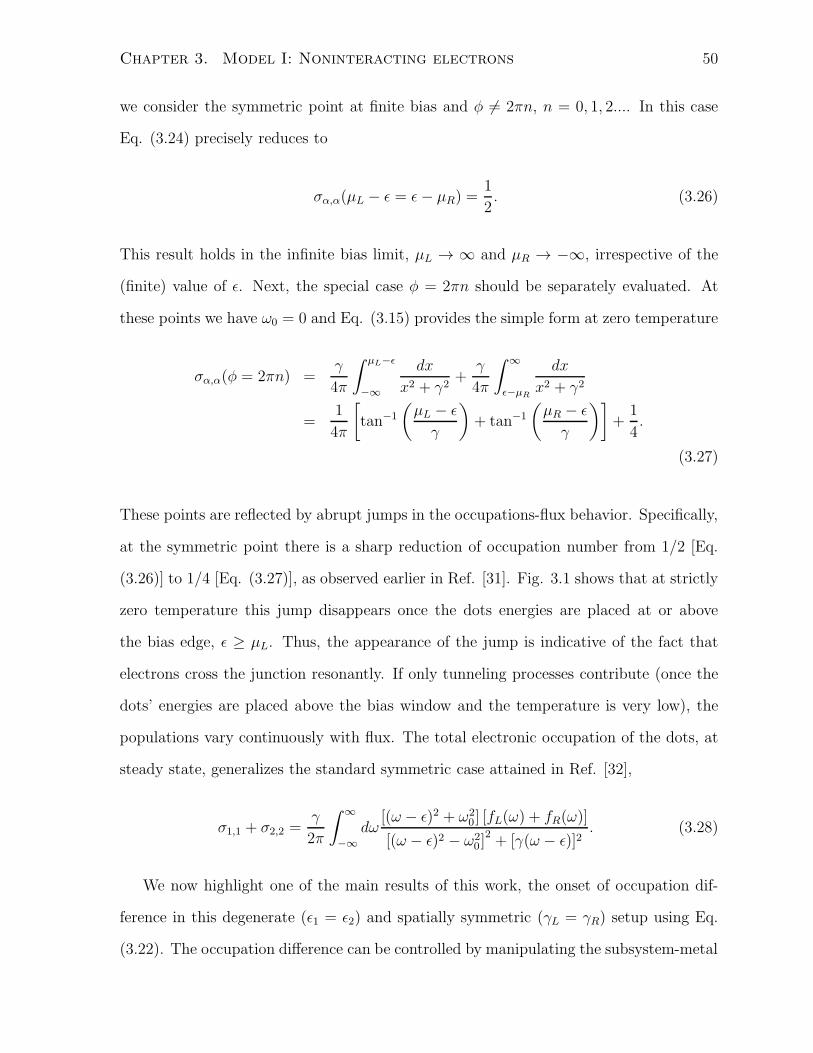
Chapter 3. Model I: Noninteracting electrons 50
we consider the symmetric point at finite bias and φ 6= 2πn, n = 0, 1, 2.... In this case
Eq. (3.24) precisely reduces to
σα,α(µL − ǫ = ǫ− µR) =1
2. (3.26)
This result holds in the infinite bias limit, µL → ∞ and µR → −∞, irrespective of the
(finite) value of ǫ. Next, the special case φ = 2πn should be separately evaluated. At
these points we have ω0 = 0 and Eq. (3.15) provides the simple form at zero temperature
σα,α(φ = 2πn) =γ
4π
∫ µL−ǫ
−∞
dx
x2 + γ2+
γ
4π
∫ ∞
ǫ−µR
dx
x2 + γ2
=1
4π
[
tan−1
(
µL − ǫ
γ
)
+ tan−1
(
µR − ǫ
γ
)]
+1
4.
(3.27)
These points are reflected by abrupt jumps in the occupations-flux behavior. Specifically,
at the symmetric point there is a sharp reduction of occupation number from 1/2 [Eq.
(3.26)] to 1/4 [Eq. (3.27)], as observed earlier in Ref. [31]. Fig. 3.1 shows that at strictly
zero temperature this jump disappears once the dots energies are placed at or above
the bias edge, ǫ ≥ µL. Thus, the appearance of the jump is indicative of the fact that
electrons cross the junction resonantly. If only tunneling processes contribute (once the
dots’ energies are placed above the bias window and the temperature is very low), the
populations vary continuously with flux. The total electronic occupation of the dots, at
steady state, generalizes the standard symmetric case attained in Ref. [32],
σ1,1 + σ2,2 =γ
2π
∫ ∞
−∞dω
[(ω − ǫ)2 + ω20] [fL(ω) + fR(ω)]
[(ω − ǫ)2 − ω20]
2+ [γ(ω − ǫ)]2
. (3.28)
We now highlight one of the main results of this work, the onset of occupation dif-
ference in this degenerate (ǫ1 = ǫ2) and spatially symmetric (γL = γR) setup using Eq.
(3.22). The occupation difference can be controlled by manipulating the subsystem-metal
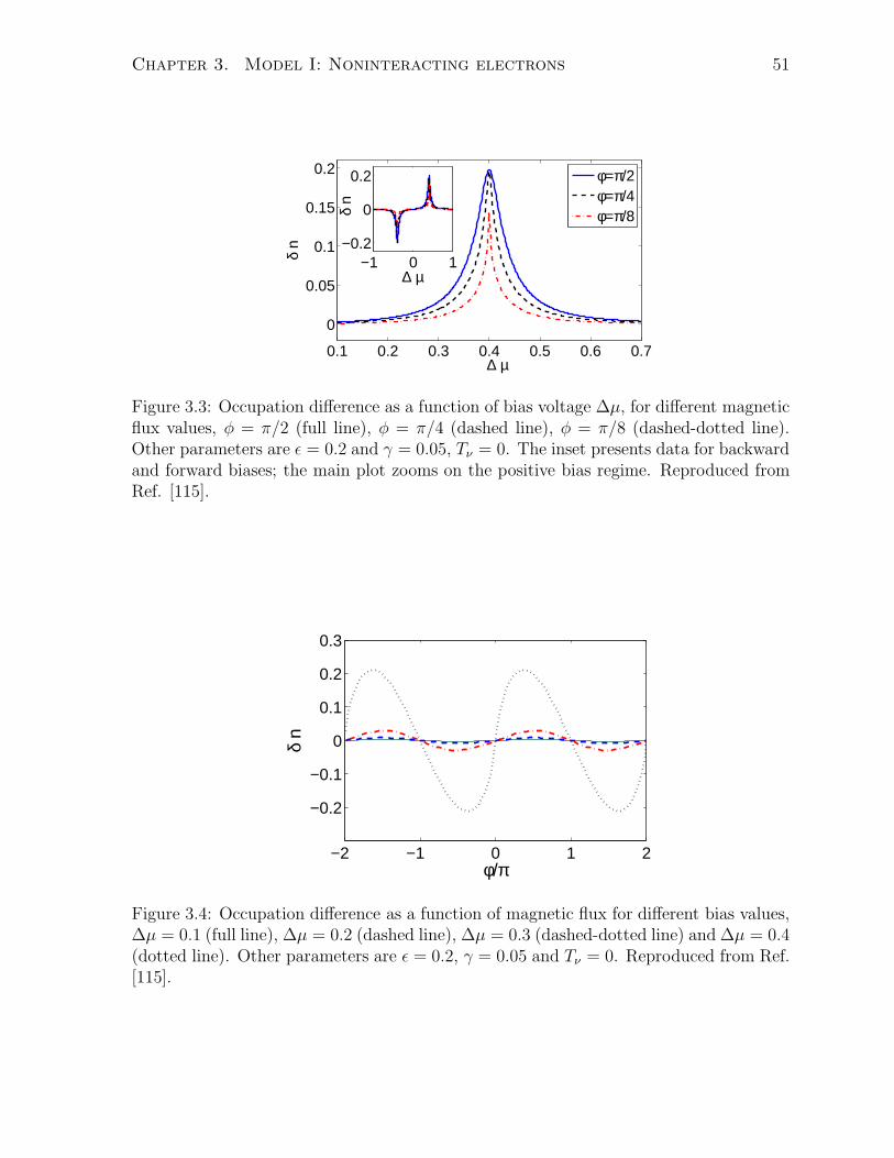
Chapter 3. Model I: Noninteracting electrons 51
0.1 0.2 0.3 0.4 0.5 0.6 0.7
0
0.05
0.1
0.15
0.2
∆ µ
δ n
−1 0 1−0.2
0
0.2
∆ µ
δ n
φ=π/2φ=π/4φ=π/8
Figure 3.3: Occupation difference as a function of bias voltage ∆µ, for different magneticflux values, φ = π/2 (full line), φ = π/4 (dashed line), φ = π/8 (dashed-dotted line).Other parameters are ǫ = 0.2 and γ = 0.05, Tν = 0. The inset presents data for backwardand forward biases; the main plot zooms on the positive bias regime. Reproduced fromRef. [115].
−2 −1 0 1 2
−0.2
−0.1
0
0.1
0.2
0.3
φ/π
δ n
Figure 3.4: Occupation difference as a function of magnetic flux for different bias values,∆µ = 0.1 (full line), ∆µ = 0.2 (dashed line), ∆µ = 0.3 (dashed-dotted line) and ∆µ = 0.4(dotted line). Other parameters are ǫ = 0.2, γ = 0.05 and Tν = 0. Reproduced from Ref.[115].
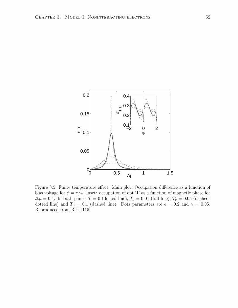
Chapter 3. Model I: Noninteracting electrons 52
0 0.5 1 1.50
0.05
0.1
0.15
0.2
∆µ
δ n −2 0 2
0.1
0.2
0.3
0.4
φ
σ 1,1
Figure 3.5: Finite temperature effect. Main plot: Occupation difference as a function ofbias voltage for φ = π/4. Inset: occupation of dot ’1’ as a function of magnetic phase for∆µ = 0.4. In both panels T = 0 (dotted line), Tν = 0.01 (full line), Tν = 0.05 (dashed-dotted line) and Tν = 0.1 (dashed line). Dots parameters are ǫ = 0.2 and γ = 0.05.Reproduced from Ref. [115].
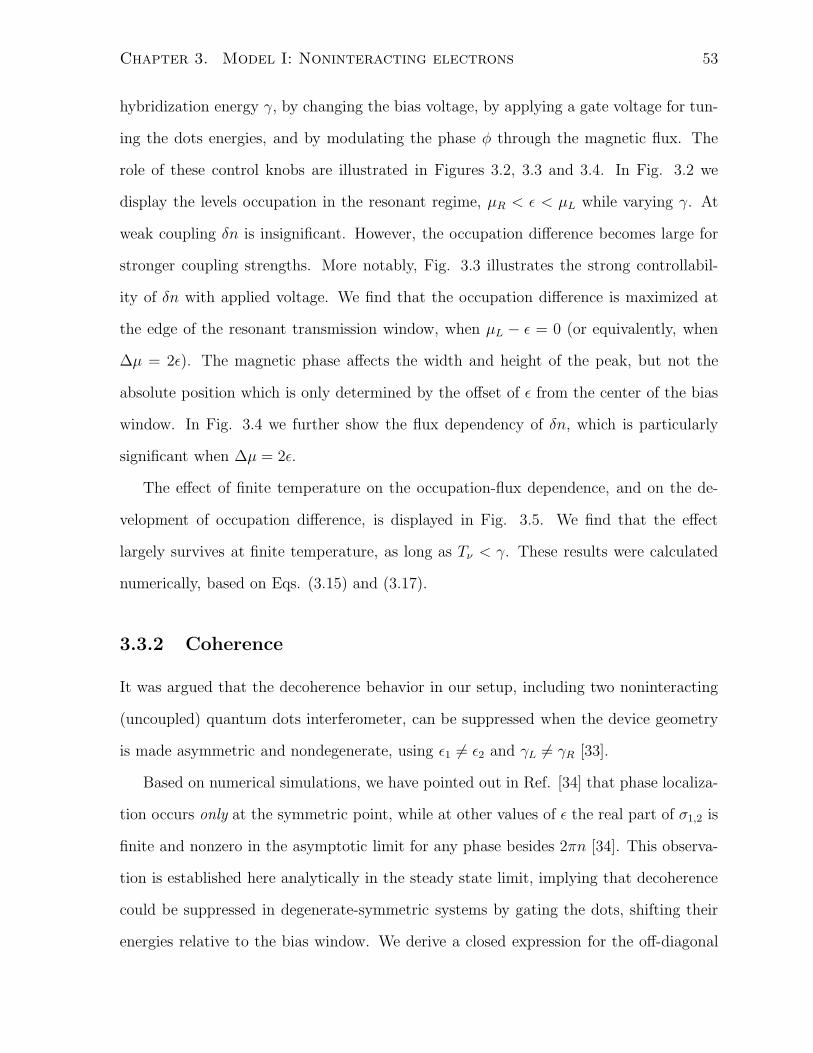
Chapter 3. Model I: Noninteracting electrons 53
hybridization energy γ, by changing the bias voltage, by applying a gate voltage for tun-
ing the dots energies, and by modulating the phase φ through the magnetic flux. The
role of these control knobs are illustrated in Figures 3.2, 3.3 and 3.4. In Fig. 3.2 we
display the levels occupation in the resonant regime, µR < ǫ < µL while varying γ. At
weak coupling δn is insignificant. However, the occupation difference becomes large for
stronger coupling strengths. More notably, Fig. 3.3 illustrates the strong controllabil-
ity of δn with applied voltage. We find that the occupation difference is maximized at
the edge of the resonant transmission window, when µL − ǫ = 0 (or equivalently, when
∆µ = 2ǫ). The magnetic phase affects the width and height of the peak, but not the
absolute position which is only determined by the offset of ǫ from the center of the bias
window. In Fig. 3.4 we further show the flux dependency of δn, which is particularly
significant when ∆µ = 2ǫ.
The effect of finite temperature on the occupation-flux dependence, and on the de-
velopment of occupation difference, is displayed in Fig. 3.5. We find that the effect
largely survives at finite temperature, as long as Tν < γ. These results were calculated
numerically, based on Eqs. (3.15) and (3.17).
3.3.2 Coherence
It was argued that the decoherence behavior in our setup, including two noninteracting
(uncoupled) quantum dots interferometer, can be suppressed when the device geometry
is made asymmetric and nondegenerate, using ǫ1 6= ǫ2 and γL 6= γR [33].
Based on numerical simulations, we have pointed out in Ref. [34] that phase localiza-
tion occurs only at the symmetric point, while at other values of ǫ the real part of σ1,2 is
finite and nonzero in the asymptotic limit for any phase besides 2πn [34]. This observa-
tion is established here analytically in the steady state limit, implying that decoherence
could be suppressed in degenerate-symmetric systems by gating the dots, shifting their
energies relative to the bias window. We derive a closed expression for the off-diagonal
Chapter 3. Model I: Noninteracting electrons 54
system element σ1,2 ≡ 〈a†1a2〉 by studying Eq. (3.9),
σ12 =γ
4π
∫ ∞
−∞fL(ω)dω
{
cos φ2[(ω − ǫ)2 − ω2
0] + i sin φ2[(ω − ǫ)2 + ω2
0]
[(ω − ǫ)2 − ω20]
2+ [γ(ω − ǫ)]2
}
+γ
4π
∫ ∞
−∞fR(ω)dω
{
cos φ2[(ω − ǫ)2 − ω2
0]− i sin φ2[(ω − ǫ)2 + ω2
0]
[(ω − ǫ)2 − ω20]
2+ [γ(ω − ǫ)]2
}
.(3.29)
At finite bias and zero temperature direct integration provides the real (ℜ) and imaginary
(ℑ) parts of σ1,2 (φ 6= 2πn),
ℜσ1,2 =1
4π
[
tan−1(µL − ǫ
γ+
)
− tan−1(µL − ǫ
γ−
)
+ tan−1(µR − ǫ
γ+
)
− tan−1(µR − ǫ
γ−
)]
,
(3.30)
and
ℑσ1,2 =sin(φ/2)
4π
[
tan−1(µL − ǫ
γ+
)
+tan−1(µL − ǫ
γ−
)
−tan−1(µR − ǫ
γ+
)
−tan−1(µR − ǫ
γ−
)]
.
(3.31)
As before, we define γ± = γ2(1 ± cos φ
2). We now readily confirm that at the symmetric
point the real part vanishes and “phase localization” takes place [31]. In particular, in
the infinite bias limit we find ℑσ1,2 = 12sin φ
2, in agreement with previous studies [34].
We also include the behavior at the special points φ = 2πn. Eq. (3.29) reduces then to
a simple Lorentzian form, at zero temperature,
σ1,2(φ = 0) =γ
4π
∫ µL−ǫ
−∞
dx
x2 + γ2+
γ
4π
∫ ∞
ǫ−µR
dx
x2 + γ2
=1
4π
[
tan−1
(
µL − ǫ
γ
)
+ tan−1
(
µR − ǫ
γ
)]
+1
4. (3.32)
The sign reverses for φ = ±2π. We note that the imaginary part of the coherence
identically vanishes at zero phase while the real part is finite, approaching the value
1/4 at the symmetric point. Numerical results in the steady state limit are displayed in
Fig. 3.6. We find that both the real and imaginary parts of σ1,2 demonstrate significant
Chapter 3. Model I: Noninteracting electrons 55
−0.2
0
0.2
ℜσ12
−2 −1 0 1 2−0.5
0
0.5
ℑσ12
∆µ
Figure 3.6: Real and imaginary parts of the coherence as a function of the bias voltage.φ = π (full line), φ = π/2 (dashed), φ = π/4 (dashed-dotted line). Other parameters areǫ = 0.2, γ = 0.05, and T = 0. The oval shape marks the region of phase localization atpositive bias. Reproduced from Ref. [115].
features when the dots’ levels cross the bias window, at ∆µ = 2ǫ. The value of the
real part abruptly changes sign, the imaginary part develops a step. At large bias ℜσ1,2
diminishes while ℑσ1,2 is finite, indicating on the development of the phase localization
behavior. It can be shown that the double-step structure of ℑσ1,2 (as a function of ∆µ)
disappears when the dots energies are set at the symmetric point.
3.3.3 Current
The electric current, flowing from the L metal to the R end, is obtained by defining
the number operator NL ≡ ∑
l a†lal, providing the current IL = −dNL
dt= −i[H, NL].
Expectation values are calculated in the steady state limit. Using the EOM formalism
as explained in Sec. 3.2, we get the standard result [116]
IL =1
2π
∫ ∞
−∞dωTL,R(ω)[fL(ω)− fR(ω)]. (3.33)
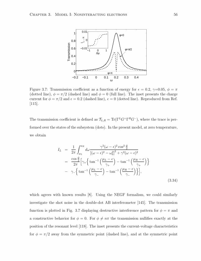
Chapter 3. Model I: Noninteracting electrons 56
−0.2 −0.1 0 0.1 0.2 0.3 0.4
0
0.2
0.4
0.6
0.8
1
ω
Tra
nsm
issi
on
φ=0
φ=π/2
φ=π
−1 0 1−0.01
0
0.01
∆µ
I L→ R
Figure 3.7: Transmission coefficient as a function of energy for ǫ = 0.2, γ=0.05, φ = π(dotted line), φ = π/2 (dashed line) and φ = 0 (full line). The inset presents the chargecurrent for φ = π/2 and ǫ = 0.2 (dashed line), ǫ = 0 (dotted line). Reproduced from Ref.[115].
The transmission coefficient is defined as TL,R = Tr(ΓLG+ΓRG−), where the trace is per-
formed over the states of the subsystem (dots). In the present model, at zero temperature,
we obtain
IL =1
2π
∫ µR
µL
dωγ2(ω − ǫ)2 cos2 φ
2
[(ω − ǫ)2 − ω20]
2+ γ2(ω − ǫ)2
=cos φ
2
2π
[
γ+
{
tan−1(µL − ǫ
γ+
)
− tan−1(µR − ǫ
γ+
)}
− γ−
{
tan−1(µL − ǫ
γ−
)
− tan−1(µR − ǫ
γ−
)}]
,
(3.34)
which agrees with known results [8]. Using the NEGF formalism, we could similarly
investigate the shot noise in the double-dot AB interferometer [145]. The transmission
function is plotted in Fig. 3.7 displaying destructive interference pattern for φ = π and
a constructive behavior for φ = 0. For φ 6= nπ the transmission nullifies exactly at the
position of the resonant level [118]. The inset presents the current-voltage characteristics
for φ = π/2 away from the symmetric point (dashed line), and at the symmetric point
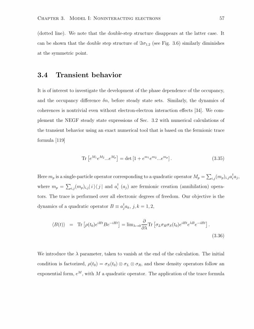
Chapter 3. Model I: Noninteracting electrons 57
(dotted line). We note that the double-step structure disappears at the latter case. It
can be shown that the double step structure of ℑσ1,2 (see Fig. 3.6) similarly diminishes
at the symmetric point.
3.4 Transient behavior
It is of interest to investigate the development of the phase dependence of the occupancy,
and the occupancy difference δn, before steady state sets. Similarly, the dynamics of
coherences is nontrivial even without electron-electron interaction effects [34]. We com-
plement the NEGF steady state expressions of Sec. 3.2 with numerical calculations of
the transient behavior using an exact numerical tool that is based on the fermionic trace
formula [119]
Tr[
eM1eM2 ...eMp]
= det [1 + em1em2 ...emp ] . (3.35)
Heremp is a single-particle operator corresponding to a quadratic operatorMp =∑
i,j(mp)i,ja†iaj ,
where mp =∑
i,j(mp)i,j| i 〉〈 j | and a†i (aj) are fermionic creation (annihilation) opera-
tors. The trace is performed over all electronic degrees of freedom. Our objective is the
dynamics of a quadratic operator B ≡ a†jak, j, k = 1, 2,
〈B(t)〉 = Tr[
ρ(t0)eiHtBe−iHt
]
= limλ→0∂
∂λTr[
σLσRσS(t0)eiHteλBe−iHt
]
.
(3.36)
We introduce the λ parameter, taken to vanish at the end of the calculation. The initial
condition is factorized, ρ(t0) = σS(t0) ⊗ σL ⊗ σR, and these density operators follow an
exponential form, eM , with M a quadratic operator. The application of the trace formula
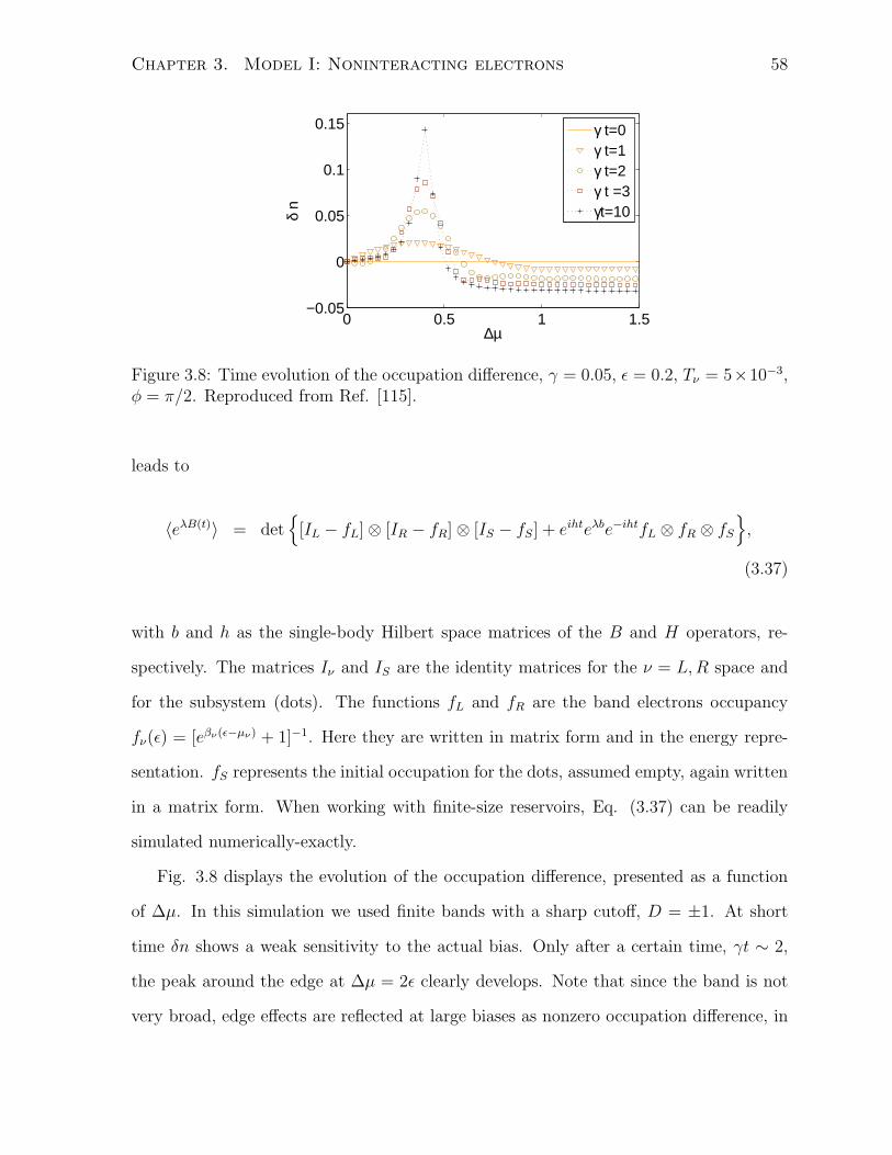
Chapter 3. Model I: Noninteracting electrons 58
0 0.5 1 1.5−0.05
0
0.05
0.1
0.15
∆µ
δ n
γ t=0γ t=1γ t=2γ t =3γt=10
Figure 3.8: Time evolution of the occupation difference, γ = 0.05, ǫ = 0.2, Tν = 5×10⁻³,φ = π/2. Reproduced from Ref. [115].
leads to
〈eλB(t)〉 = det{
[IL − fL]⊗ [IR − fR]⊗ [IS − fS] + eihteλbe−ihtfL ⊗ fR ⊗ fS
}
,
(3.37)
with b and h as the single-body Hilbert space matrices of the B and H operators, re-
spectively. The matrices Iν and IS are the identity matrices for the ν = L,R space and
for the subsystem (dots). The functions fL and fR are the band electrons occupancy
fν(ǫ) = [eβν(ǫ−µν) + 1]−1. Here they are written in matrix form and in the energy repre-
sentation. fS represents the initial occupation for the dots, assumed empty, again written
in a matrix form. When working with finite-size reservoirs, Eq. (3.37) can be readily
simulated numerically-exactly.
Fig. 3.8 displays the evolution of the occupation difference, presented as a function
of ∆µ. In this simulation we used finite bands with a sharp cutoff, D = ±1. At short
time δn shows a weak sensitivity to the actual bias. Only after a certain time, γt ∼ 2,
the peak around the edge at ∆µ = 2ǫ clearly develops. Note that since the band is not
very broad, edge effects are reflected at large biases as nonzero occupation difference, in
Chapter 3. Model I: Noninteracting electrons 59
0
0.1
ℜ σ
1,2
(a)
0 0.5 1 1.5
0
0.2
0.4
∆µ
ℑ σ
1,2
(b)
γ t=0
γ t=1
γ t=2
γ t =3
γ t=5
γ t=7
γt=10
Figure 3.9: Time evolution of the real (a) and imaginary (b) parts of the coherenceγ = 0.05, ǫ = 0.2, Tν = 5× 10⁻³, φ = π/2. Reproduced from Ref. [115].
contrast to the broad-bandwidth long-time behavior of Fig. 3.3.
The transient behavior of the coherences, ℜσ1,2 and ℑσ1,2, is included in Fig. 3.9; the
corresponding steady state value are presented in Fig. 3.6. We can follow the temporal
features of the phase localization effect, i.e., the disappearance of the real part of the
coherence at the symmetric point or at large bias, when φ 6= 2πn. Using φ = π/2 we
note that while at short to intermediate time (γt < 2) significant coherence builds up, the
real part of the coherence eventually survives only at small biases. Regarding timescales,
we find that while ℑσ1,2 reaches the steady state values at short time, γt ∼ 2, ℜσ1,2
approaches its stationary limit only at longer times, for γt ∼ 10. Similar results were
obtained in Ref. [34].
3.5 Dephasing
Phase-breaking processes arise due to the interaction of electrons with other degrees of
freedom, e.g., with electrons, phonons and defects. We extend here the discussion of Sec.
3.3 and incorporate dephasing processes into our system phenomenologically, by using the
well established method of Buttiker dephasing probe [66]. The schematic setup is shown
Chapter 3. Model I: Noninteracting electrons 60
in Fig. 2.2. In this technique, elastic dephasing processes on the dots are emulated by
including a third terminal, P , enforcing the requirement that the charge current towards
the probe terminal, at a given electron energy, should vanish. Thus, electrons travel to
the probe and return to the system with a different phase, while both electron number
and electron energy are conserved. This condition sets an electron distribution within
the probe. As we show below, away from the symmetric point this distribution effectively
depends on the magnetic phase. Following the equations-of-motion approach as detailed
in Sec. 3.2, we arrive at the steady-state expression for the reduced density matrix
〈a†αaβ〉 =1
2π
∑
ν=L,R,P
∫ ∞
−∞
(
G+ΓνG−)
α,βfν(ω)dω. (3.38)
The probe hybridization matrix is given by
ΓP = γP
1 0
0 0
, (3.39)
and the dot’s Green’s function is written by generalizing the matrix (3.12), to include
the probe self energy,
G+ =
ω − ǫ1 +i(γL+γR+γP )
2iγL2eiφ/2 + iγR
2e−iφ/2
iγL2e−iφ/2 + iγR
2eiφ/2 ω − ǫ2 +
i(γL+γR)2
−1
.
This matrix is written here in a general form, to allow one to distinguish between the
two dots and the different dots-metals hybridization terms. The dot-probe hybridization
is defined as γP = 2π∑
p |λp|2δ(ω − ωp), in analogy with Eq. (5.45). In our calculations
below we assume energy degenerate dots and symmetric couplings, ǫ = ǫ1 = ǫ2, γL =
γR = γ/2. We now derive the probe distribution by demanding that the energy resolved
charge current to the P terminal vanishes. The total current to P is given by the sum
Chapter 3. Model I: Noninteracting electrons 61
of the currents from the L and R terminals, generalizing Eq. (3.33),
IP = IL→P + IR→P
=1
2π
∫ ∞
−∞[TL,P (ω, φ)fL(ω)− TP,L(ω, φ)fP (ω, φ)] dω
+1
2π
∫ ∞
−∞[TR,P (ω, φ)fR(ω)− TP,R(ω, φ)fP (ω, φ)]dω (3.40)
with the transmission coefficient Tν,ν(ω) = Tr[ΓνG+ΓνG−]. By requiring the integrand
to vanish, we arrive at the probe distribution
fP (ω, φ) =TL,P (ω, φ)fL(ω) + TR,P (ω, φ)fR(ω)
TL,P (ω, φ) + TR,P (ω, φ). (3.41)
Direct evaluation of these transmission coefficients provide the electron distribution in
the probe,
fP (ω, φ) =fL(ω) + fR(ω)
2+
γ(ω − ǫ) sin φ2cos φ
2
2[(ω − ǫ)2 + ω20]
[fL(ω)− fR(ω)] . (3.42)
As before, ω0 = γ2sin φ
2. This expression indicates that the magnetic flux plays a role
in setting the distribution within the probe, (such that it only dephases the system and
does not deplete electrons or allow energy reorganization). This dependence disappears
when the dots’ energies are set at the symmetric point, since the contribution of the
second term in Eq. (3.42) diminishes in the integrals of Eq. (3.43), from symmetry
considerations. We now write integral expressions for the dots occupations using Eq.
Chapter 3. Model I: Noninteracting electrons 62
(3.38),
σ1,1 =γ
4π
∫ ∞
−∞
dω
∆(ω)
{
[
(ω − ǫ)2 + ω20 − 2ω0(ω − ǫ) cos
φ
2
]
fL(ω)
+
[
(ω − ǫ)2 + ω20 + 2ω0(ω − ǫ) cos
φ
2
]
fR(ω)
}
+γP2π
∫ ∞
−∞
dω
∆(ω)
[
(ω − ǫ)2 +γ2
4
]
fP (ω)
σ2,2 =γ
4π
∫ ∞
−∞
dω
∆(ω)
{
[
(ω − ǫ)2 + ω20 + 2ω0(ω − ǫ) cos
φ
2+ ω0γP sin
φ
2+
γ2P
4
]
fL(ω)
+
[
(ω − ǫ)2 + ω20 − 2ω0(ω − ǫ) cos
φ
2+ ω0γP sin
φ
2+
γ2P
4
]
fR(ω)
}
+γ2γP8π
cos2φ
2
∫ ∞
−∞
dω
∆(ω)fP (ω), (3.43)
with
∆(ω) =∣
∣
∣(ω − ǫ)2 − ω2
0 −γγP4
+ i(
γ +γP2
)
(ω − ǫ)∣
∣
∣
2
.
In the absence of dephasing these expressions reduce to Eqs. (3.15) and (3.17). In
the opposite limit, at very large dephasing, γP ≫ γ, γP > ∆µ, we note that σ2,2 is
dominated by γ2Pγ terms that are flux independent, while σ1,1 is dominated by its last
term, ∝ γPfP , which is flux dependent away from the symmetric point, resulting in
σ1,1 ∝ sin(φ). Thus, quite counter-intuitively, we find that the level that is directly
susceptible to local dephasing demonstrates flux dependency of occupation at strong
dephasing, while the level that indirectly suffers dephasing effects more feasibly loses its
coherent oscillations.
Using numerical integration, dots occupations and their oscillation with phase are
presented in Fig. 3.10. We observe the following trends upon increasing dephasing
strength: At the symmetric point, panels (a)-(b), the abrupt jump at zero magnetic
phase immediately disappears with the application of finite dephasing. When the dot
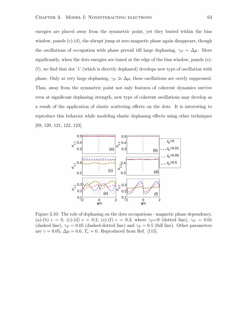
Chapter 3. Model I: Noninteracting electrons 63
energies are placed away from the symmetric point, yet they buried within the bias
window, panels (c)-(d), the abrupt jump at zero magnetic phase again disappears, though
the oscillations of occupation with phase prevail till large dephasing, γP ∼ ∆µ. More
significantly, when the dots energies are tuned at the edge of the bias window, panels (e)-
(f), we find that dot ’1’ (which is directly dephased) develops new type of oscillation with
phase. Only at very large dephasing, γP ≫ ∆µ, these oscillations are overly suppressed.
Thus, away from the symmetric point not only features of coherent dynamics survive
even at significant dephasing strength, new type of coherent oscillations may develop as
a result of the application of elastic scattering effects on the dots. It is interesting to
reproduce this behavior while modeling elastic dephasing effects using other techniques
[69, 120, 121, 122, 123].
0.3
0.4
0.5
σ 1,1
(a) 0.3
0.4
0.5
σ 2,2
(b)
0.2
0.4
σ 1,1
(c)0.2
0.4
σ 2,2
(d)
−2 0 20.1
0.2
0.3
φ/π
σ 1,1
(e)
−2 0 20.1
0.2
0.3
φ/π
σ 2,2
(f)
γP=0
γP=0.01
γP=0.05
γP=0.5
Figure 3.10: The role of dephasing on the dots occupations - magnetic phase dependency,(a)-(b) ǫ = 0, (c)-(d) ǫ = 0.2, (e)-(f) ǫ = 0.3, where γP=0 (dotted line), γP = 0.01(dashed line), γP = 0.05 (dashed-dotted line) and γP = 0.5 (full line). Other parametersare γ = 0.05, ∆µ = 0.6, Tν = 0. Reproduced from Ref. [115].
Chapter 3. Model I: Noninteracting electrons 64
3.6 Discussion
In this chapter, we have addressed the issue of magnetic field control on electronic oc-
cupation and coherence in the noninteracting double-dot AB interferometers, model I
and model II. The system under investigation included energy degenerate dots with sym-
metric dot-metals hybridization strengths. However, by voltage gating the dots’ energies
away from the so-called symmetric point at which ǫ = (µL + µR)/2 we have resolved
three nontrivial effects that can allow for significant controllability over dots’ occupation
and their coherence: (i) Dots’ occupations may significantly vary with magnetic flux,
particularly when the levels reside close to the bias edge. (ii) The dots acquire different
occupations, though they are energy degenerate. This behavior is maximized at the bias
edge ǫ ∼ µL. It survives at finite temperature, as long as T < γ. (iii) Regarding the
dots’ coherence, we have proven that the effect of “phase localization” [31] does not take
place away from the symmetric point, allowing for coherence control in the system.
Our minimal model could be applied to describe magnetic field control in mesoscopic
conducting loops and in molecular ring structures. In the latter case it was particularly
noted that degeneracy is crucial for allowing controllability within realistic magnetic fields
[13]. We also considered the effect of dephasing on dot occupations and demonstrated
that the system can withstand dephasing under certain conditions. The results resolved
here could be useful for constructing two qubit gates and long-lived memory elements.
This study was limited to the noninteracting electron model, excluding electron-
electron interaction effects. In the next chapter we study the transient dynamics of
coherences and the charge current, taking into account finite electron-electron repulsion.
We also discuss the limit of a very strong U where double occupancy is forbidden.
Chapter 4
Model I interacting case: Coherence
dynamics
4.1 Introduction
The focus of this chapter is the detailed study of the dynamical role of finite electron-
electron interactions on the intrinsic coherence behaviour in a biased double-dot AB
interferometer, in model I. The system includes a parallel quantum dot setup for the AB
interferometer, where (spinless) electrons experience an inter-dot repulsion effect. For a
schematic representation, see Fig. 2.1. We focus on the dynamics of the coherences, off-
diagonal elements of the double-dot reduced density matrix. Furthermore, we simulate
the charge current in the system, assuming different values for the magnetic flux. Other
effects considered are the role of finite temperature on the coherence pattern, and the
behaviour away from the electron-hole symmetric point, a regime not considered before
in a non-perturbative calculation within the AB setup [124]. Results presented in this
chapter were published in Ref. [34].
Our simulations show that general dynamical characteristics of the double-dot co-
herence are maintained upon the application of inter-dot Coulombic interactions. In
65
Chapter 4. Model I interacting case: Coherence dynamics 66
particular, the characteristic timescale for reaching the steady state limit, the depen-
dence of the coherence on the AB phase factors, and the form of the temporal current,
similarly evolve for systems at zero or finite inter-dot interaction, for finite bias (beyond
linear response), away from the electron-hole symmetric point, at low or high tempera-
tures. We compare our data to (analytic) results based on a master equation treatment.
This method can readily handle the zero electron-electron interaction case and the op-
posite case, the infinite interaction limit. Interestingly, in the latter Coulomb blockade
limit the coherence is expected to evolve and sustain values distinctively different from
its behaviour at finite interactions.
4.2 Model I
We focus on the symmetric AB setup, with a quantum dot located at each arm of the
interferometer, see Fig. 2.1. The dots are each connected to two metal leads, maintained
in a biased state. The dots ’1’ and ’2’ are represented by the electronic levels ǫ1, and
ǫ2, respectively, described by the creation (annihilation) operators a†β (aβ), where β =
1, 2. These levels are coupled in an AB geometry to two metal leads (ν = L,R) with
chemical potentials µν . For a schematic representation see Fig. 2.1. Here we include the
Hamiltonian of model I and the definitions, since we use slightly different convention for
the hydridization. The total Hamiltonian, HAB, has the form,
HAB = HS +HB +HSB, (4.1)
where HS corresponds to the isolated dot Hamiltonian,
HS = ǫ1a†1a1 + ǫ2a
†2a2 + Ua†1a1a
†2a2. (4.2)
Chapter 4. Model I interacting case: Coherence dynamics 67
HB include the left and right leads,
HB =∑
l
ωla†lal +
∑
r
ωra†rar, (4.3)
and HSB stands for the dot-lead tunneling term,
HSB =∑
β,l
ξβ,la†βale
iφLβ +
∑
β,r
ζβ,ra†raβe
iφRβ + h.c. (4.4)
Here ξβ,l and ζβ,r are real numbers. The hybridization matrix elements between the dot
and the left/right leads are,
ΓLβ,β′(ω) = 2πe
i(φLβ−φL
β′)∑
l
ξβ,lδ(ω − ωl)ξ∗β′,l, (4.5)
ΓRβ,β′(ω) = 2πe
−i(φRβ −φR
β′)∑
r
ζβ,rδ(ω − ωr)ζ∗β′,r. (4.6)
We assume that level one and two couple identically with left (L) lead and write the
diagonal element of hybridization matrix ΓL as,
γL = π∑
l
(ξl,β)2δ(ω − ωl), (4.7)
and similarly to the right (R),
γR = π∑
r
(ζr,β)2δ(ω − ωr). (4.8)
The total diagonal decay is identified by Γ = γL + γR. Further, in what follows we only
consider a degenerate situation with ǫ ≡ ǫβ , and the dots are symmetrically coupled to
both the leads. Using the INFPI approach, the following observables could be followed:
the dots’ occupation, 〈nβ〉 ≡ Tr[a†βaβρ], the coherence, σ1,2 ≡ Tr[a†1a2ρ], and the total
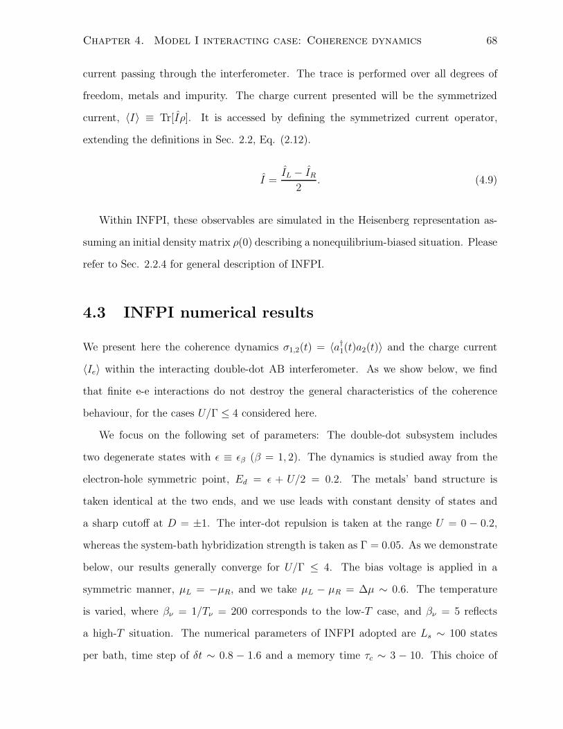
Chapter 4. Model I interacting case: Coherence dynamics 68
current passing through the interferometer. The trace is performed over all degrees of
freedom, metals and impurity. The charge current presented will be the symmetrized
current, 〈I〉 ≡ Tr[Iρ]. It is accessed by defining the symmetrized current operator,
extending the definitions in Sec. 2.2, Eq. (2.12).
I =IL − IR
2. (4.9)
Within INFPI, these observables are simulated in the Heisenberg representation as-
suming an initial density matrix ρ(0) describing a nonequilibrium-biased situation. Please
refer to Sec. 2.2.4 for general description of INFPI.
4.3 INFPI numerical results
We present here the coherence dynamics σ1,2(t) = 〈a†1(t)a2(t)〉 and the charge current
〈Ie〉 within the interacting double-dot AB interferometer. As we show below, we find
that finite e-e interactions do not destroy the general characteristics of the coherence
behaviour, for the cases U/Γ ≤ 4 considered here.
We focus on the following set of parameters: The double-dot subsystem includes
two degenerate states with ǫ ≡ ǫβ (β = 1, 2). The dynamics is studied away from the
electron-hole symmetric point, Ed = ǫ + U/2 = 0.2. The metals’ band structure is
taken identical at the two ends, and we use leads with constant density of states and
a sharp cutoff at D = ±1. The inter-dot repulsion is taken at the range U = 0 − 0.2,
whereas the system-bath hybridization strength is taken as Γ = 0.05. As we demonstrate
below, our results generally converge for U/Γ ≤ 4. The bias voltage is applied in a
symmetric manner, µL = −µR, and we take µL − µR = ∆µ ∼ 0.6. The temperature
is varied, where βν = 1/Tν = 200 corresponds to the low-T case, and βν = 5 reflects
a high-T situation. The numerical parameters of INFPI adopted are Ls ∼ 100 states
per bath, time step of δt ∼ 0.8 − 1.6 and a memory time τc ∼ 3 − 10. This choice of
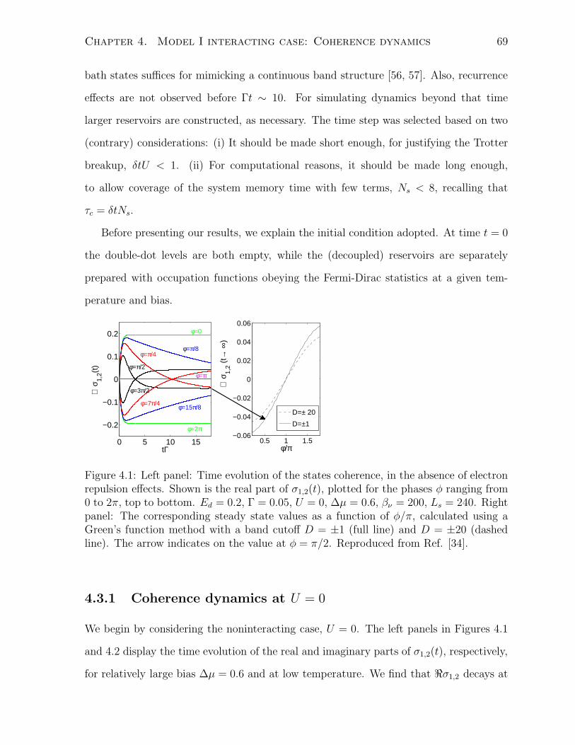
Chapter 4. Model I interacting case: Coherence dynamics 69
bath states suffices for mimicking a continuous band structure [56, 57]. Also, recurrence
effects are not observed before Γt ∼ 10. For simulating dynamics beyond that time
larger reservoirs are constructed, as necessary. The time step was selected based on two
(contrary) considerations: (i) It should be made short enough, for justifying the Trotter
breakup, δtU < 1. (ii) For computational reasons, it should be made long enough,
to allow coverage of the system memory time with few terms, Ns < 8, recalling that
τc = δtNs.
Before presenting our results, we explain the initial condition adopted. At time t = 0
the double-dot levels are both empty, while the (decoupled) reservoirs are separately
prepared with occupation functions obeying the Fermi-Dirac statistics at a given tem-
perature and bias.
0 5 10 15
−0.2
−0.1
0
0.1
0.2 φ=0
φ=π/8φ=π/4
φ=π/2φ=π
φ=2π
φ=15π/8φ=7π/4
φ=3π/2
tΓ
ℜ σ
1,2(t
)
0.5 1 1.5−0.06
−0.04
−0.02
0
0.02
0.04
0.06
φ/π
ℜ σ
1,2 (
t→ ∞
)
D=± 20
D=±1
Figure 4.1: Left panel: Time evolution of the states coherence, in the absence of electronrepulsion effects. Shown is the real part of σ1,2(t), plotted for the phases φ ranging from0 to 2π, top to bottom. Ed = 0.2, Γ = 0.05, U = 0, ∆µ = 0.6, βν = 200, Ls = 240. Rightpanel: The corresponding steady state values as a function of φ/π, calculated using aGreen’s function method with a band cutoff D = ±1 (full line) and D = ±20 (dashedline). The arrow indicates on the value at φ = π/2. Reproduced from Ref. [34].
4.3.1 Coherence dynamics at U = 0
We begin by considering the noninteracting case, U = 0. The left panels in Figures 4.1
and 4.2 display the time evolution of the real and imaginary parts of σ1,2(t), respectively,
for relatively large bias ∆µ = 0.6 and at low temperature. We find that ℜσ1,2 decays at
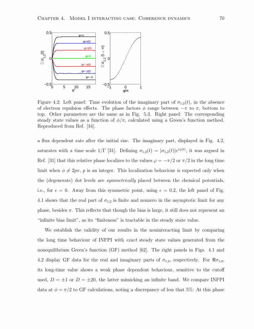
Chapter 4. Model I interacting case: Coherence dynamics 70
0 5 10 15−0.5
0
0.5
φ=0
φ=π/4
φ=π/2
φ=π
φ=−π
φ=−π/2
φ=−π/4
tΓ
ℑ σ
1,2(t
)
−1 0 1−0.5
0
0.5
φ/π
ℑ σ
1,2 (
t→ ∞
)Figure 4.2: Left panel: Time evolution of the imaginary part of σ1,2(t), in the absenceof electron repulsion effects. The phase factors φ range between −π to π, bottom totop. Other parameters are the same as in Fig. 5.3. Right panel: The correspondingsteady state values as a function of φ/π, calculated using a Green’s function method.Reproduced from Ref. [34].
a flux dependent rate after the initial rise. The imaginary part, displayed in Fig. 4.2,
saturates with a time scale 1/Γ [31]. Defining σ1,2(t) = |σ1,2(t)|eiϕ(t), it was argued in
Ref. [31] that this relative phase localizes to the values ϕ = −π/2 or π/2 in the long time
limit when φ 6= 2pπ, p is an integer. This localization behaviour is expected only when
the (degenerate) dot levels are symmetrically placed between the chemical potentials,
i.e., for ǫ = 0. Away from this symmetric point, using ǫ = 0.2, the left panel of Fig.
4.1 shows that the real part of σ1,2 is finite and nonzero in the asymptotic limit for any
phase, besides π. This reflects that though the bias is large, it still does not represent an
“infinite bias limit”, as its “finiteness” is tractable in the steady state value.
We establish the validity of our results in the noninteracting limit by comparing
the long time behaviour of INFPI with exact steady state values generated from the
nonequilibrium Green’s function (GF) method [62]. The right panels in Figs. 4.1 and
4.2 display GF data for the real and imaginary parts of σ1,2, respectively. For ℜσ1,2,
its long-time value shows a weak phase dependent behaviour, sensitive to the cutoff
used, D = ±1 or D = ±20, the latter mimicking an infinite band. We compare INFPI
data at φ = π/2 to GF calculations, noting a discrepancy of less that 5%: At this phase
Chapter 4. Model I interacting case: Coherence dynamics 71
ℜσ1,2(tΓ = 15) = −0.041 with INFPI, whereas GF calculations (arrow) yield−0.043. The
behaviour of ℑσ1,2 was found to be practically insensitive to the cutoff used, D = ±1 or
D = ±20. Overall, Green’s function simulations and INFPI results agree within 1.5% for
ℑσ1,2. Deviations between the methods should diminish when running INFPI simulations
with more states per electronic bath.
0 1 2 30
0.05
0.1
0.15
0.2
0.25
tΓ
ℜ σ
1,2(t
)
φ=0
φ=π/2
0 1 2 30
0.5
tΓ
ℑ σ
1,2(t
)
φ=π
Figure 4.3: Time evolution of σ1,2 for U = 0 (full line), U = 0.1 (dashed line) andU = 0.2 (dotted line). Main: Real part of σ1,2(t). The three top lines were simulated forφ = 0. The bottom lines were obtained using φ = π/2. The numerical parameters areδt = 1, Ns = 6 and Ls = 120. Inset: Imaginary part of σ1,2(t) when φ = π. Numericalparameters are δt = 1.6, Ns = 6 and Ls = 120. Other parameters are Ed = 0.2, Γ = 0.05,∆µ = 0.6 and βν = 200. Reproduced from Ref. [34].
4.3.2 Coherence and current at finite U
We now investigate the role of e-e repulsion effects on the coherence behaviour. Fig. 4.3
displays the real part of σ1,2(t) for two phases, φ = 0 and φ = π/2, and its imaginary
part for φ = π (inset), for three values of U . Data for ℑσ1,2(t) at U = 0.2 has not
converged for the τc adopted, see text following Fig. 4.9. In comparison to the U = 0
case, we find that general trends are maintained, though the long time coherences are
larger in the finite U case. Note our convention: the parameter Ed = ǫ+U/2 is taken as
fixed between simulations with different values of U . The trajectory simulated extends
up to Γt = 3, where convergence is satisfactory. Different memory times were used for
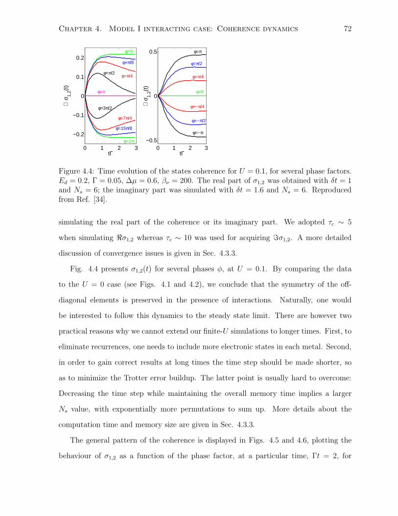
Chapter 4. Model I interacting case: Coherence dynamics 72
0 1 2 3
−0.2
−0.1
0
0.1
0.2φ=0
φ=π/8
φ=π/4φ=π/2
φ=π
φ=2π
φ=15π/8
φ=7π/4
φ=3π/2
tΓ
ℜ σ
1,2(t
)
0 1 2 3−0.5
0
0.5
φ=0
φ=π/4
φ=π/2
φ=π
φ=−π/4
φ=−π/2
φ=−π
tΓℑ
σ1,
2(t)
Figure 4.4: Time evolution of the states coherence for U = 0.1, for several phase factors.Ed = 0.2, Γ = 0.05, ∆µ = 0.6, βν = 200. The real part of σ1,2 was obtained with δt = 1and Ns = 6; the imaginary part was simulated with δt = 1.6 and Ns = 6. Reproducedfrom Ref. [34].
simulating the real part of the coherence or its imaginary part. We adopted τc ∼ 5
when simulating ℜσ1,2 whereas τc ∼ 10 was used for acquiring ℑσ1,2. A more detailed
discussion of convergence issues is given in Sec. 4.3.3.
Fig. 4.4 presents σ1,2(t) for several phases φ, at U = 0.1. By comparing the data
to the U = 0 case (see Figs. 4.1 and 4.2), we conclude that the symmetry of the off-
diagonal elements is preserved in the presence of interactions. Naturally, one would
be interested to follow this dynamics to the steady state limit. There are however two
practical reasons why we cannot extend our finite-U simulations to longer times. First, to
eliminate recurrences, one needs to include more electronic states in each metal. Second,
in order to gain correct results at long times the time step should be made shorter, so
as to minimize the Trotter error buildup. The latter point is usually hard to overcome:
Decreasing the time step while maintaining the overall memory time implies a larger
Ns value, with exponentially more permutations to sum up. More details about the
computation time and memory size are given in Sec. 4.3.3.
The general pattern of the coherence is displayed in Figs. 4.5 and 4.6, plotting the
behaviour of σ1,2 as a function of the phase factor, at a particular time, Γt = 2, for
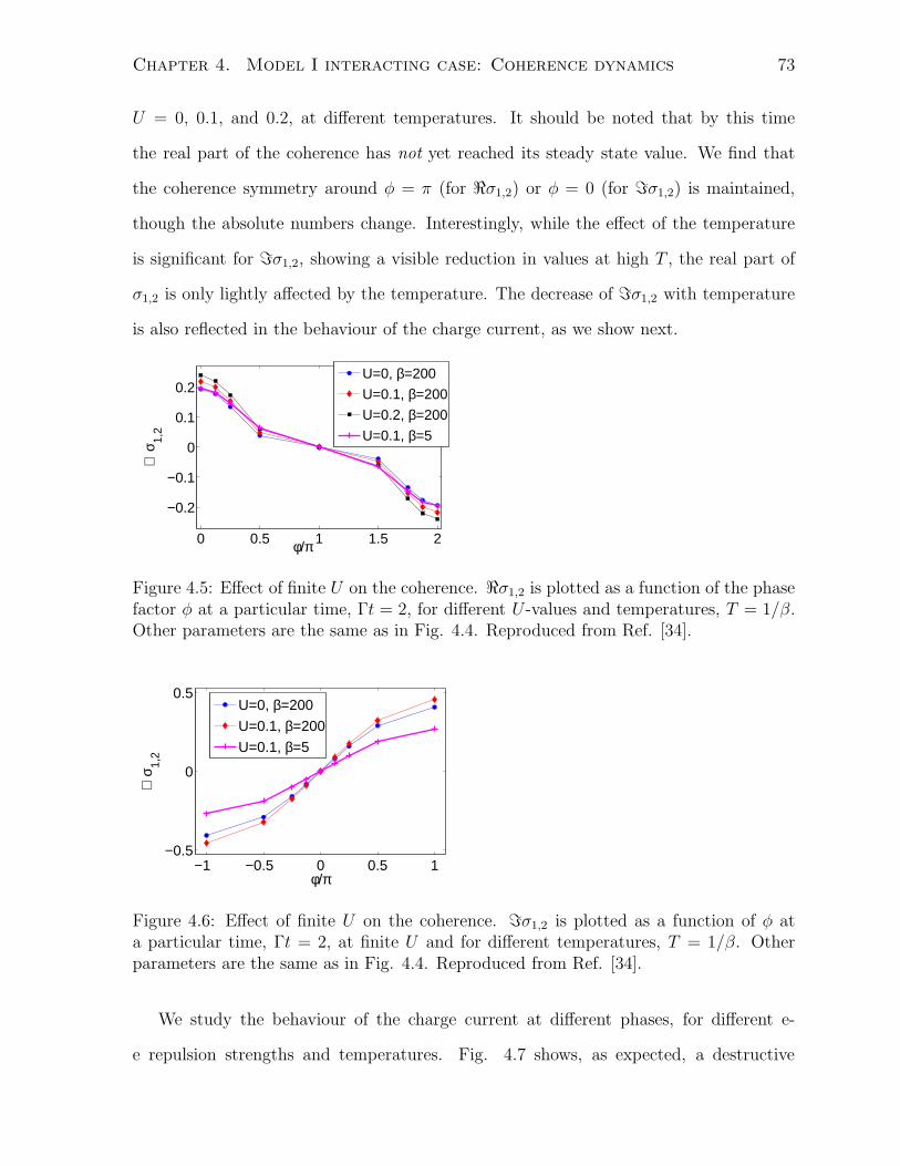
Chapter 4. Model I interacting case: Coherence dynamics 73
U = 0, 0.1, and 0.2, at different temperatures. It should be noted that by this time
the real part of the coherence has not yet reached its steady state value. We find that
the coherence symmetry around φ = π (for ℜσ1,2) or φ = 0 (for ℑσ1,2) is maintained,
though the absolute numbers change. Interestingly, while the effect of the temperature
is significant for ℑσ1,2, showing a visible reduction in values at high T , the real part of
σ1,2 is only lightly affected by the temperature. The decrease of ℑσ1,2 with temperature
is also reflected in the behaviour of the charge current, as we show next.
0 0.5 1 1.5 2
−0.2
−0.1
0
0.1
0.2
φ/π
ℜ σ
1,2
U=0, β=200
U=0.1, β=200
U=0.2, β=200
U=0.1, β=5
Figure 4.5: Effect of finite U on the coherence. ℜσ1,2 is plotted as a function of the phasefactor φ at a particular time, Γt = 2, for different U -values and temperatures, T = 1/β.Other parameters are the same as in Fig. 4.4. Reproduced from Ref. [34].
−1 −0.5 0 0.5 1−0.5
0
0.5
φ/π
ℑ σ
1,2
U=0, β=200
U=0.1, β=200
U=0.1, β=5
Figure 4.6: Effect of finite U on the coherence. ℑσ1,2 is plotted as a function of φ ata particular time, Γt = 2, at finite U and for different temperatures, T = 1/β. Otherparameters are the same as in Fig. 4.4. Reproduced from Ref. [34].
We study the behaviour of the charge current at different phases, for different e-
e repulsion strengths and temperatures. Fig. 4.7 shows, as expected, a destructive
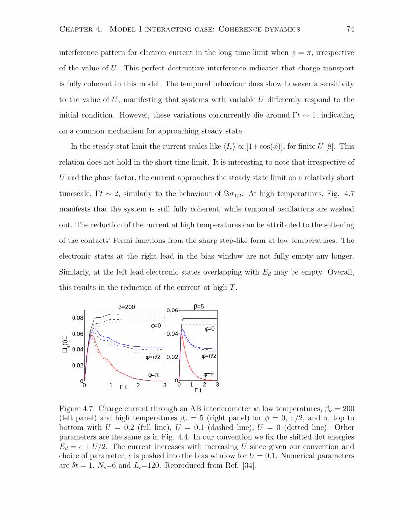
Chapter 4. Model I interacting case: Coherence dynamics 74
interference pattern for electron current in the long time limit when φ = π, irrespective
of the value of U . This perfect destructive interference indicates that charge transport
is fully coherent in this model. The temporal behaviour does show however a sensitivity
to the value of U , manifesting that systems with variable U differently respond to the
initial condition. However, these variations concurrently die around Γt ∼ 1, indicating
on a common mechanism for approaching steady state.
In the steady-stat limit the current scales like 〈Ie〉 ∝ [1+cos(φ)], for finite U [8]. This
relation does not hold in the short time limit. It is interesting to note that irrespective of
U and the phase factor, the current approaches the steady state limit on a relatively short
timescale, Γt ∼ 2, similarly to the behaviour of ℑσ1,2. At high temperatures, Fig. 4.7
manifests that the system is still fully coherent, while temporal oscillations are washed
out. The reduction of the current at high temperatures can be attributed to the softening
of the contacts’ Fermi functions from the sharp step-like form at low temperatures. The
electronic states at the right lead in the bias window are not fully empty any longer.
Similarly, at the left lead electronic states overlapping with Ed may be empty. Overall,
this results in the reduction of the current at high T .
0 1 2 30
0.02
0.04
0.06
0.08
Γ t
⟨ Ie(t
)⟩
φ=0
φ=π/2
φ=π
0 1 2 30
0.02
0.04
0.06
Γ t
φ=0
φ=π/2
φ=π
β=5β=200
Figure 4.7: Charge current through an AB interferometer at low temperatures, βν = 200(left panel) and high temperatures βν = 5 (right panel) for φ = 0, π/2, and π, top tobottom with U = 0.2 (full line), U = 0.1 (dashed line), U = 0 (dotted line). Otherparameters are the same as in Fig. 4.4. In our convention we fix the shifted dot energiesEd = ǫ + U/2. The current increases with increasing U since given our convention andchoice of parameter, ǫ is pushed into the bias window for U = 0.1. Numerical parametersare δt = 1, Ns=6 and Ls=120. Reproduced from Ref. [34].
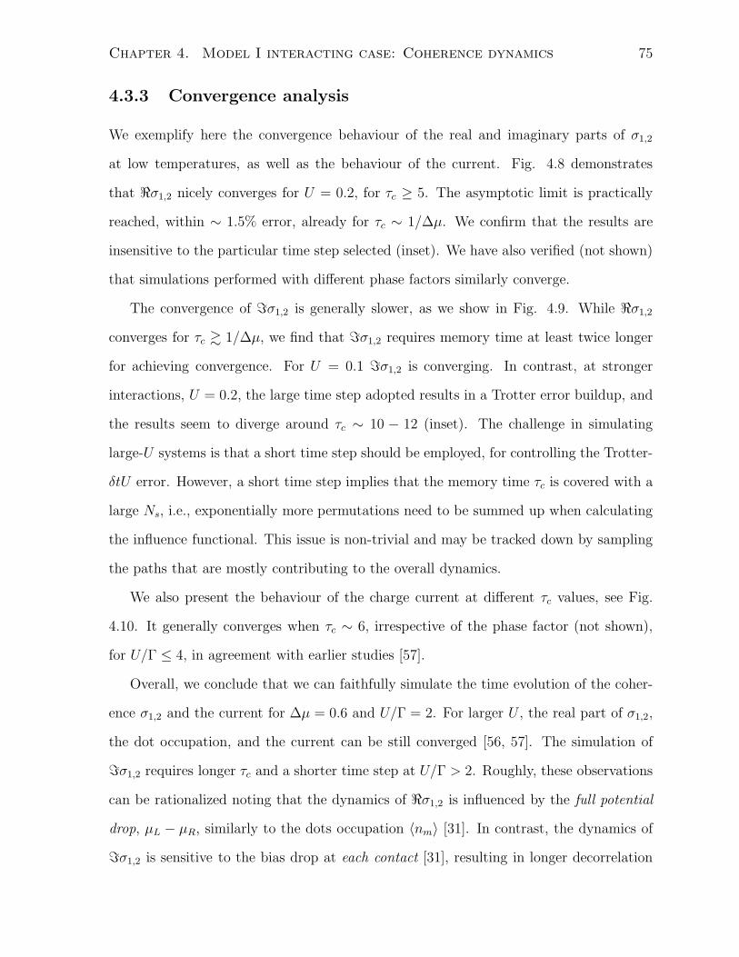
Chapter 4. Model I interacting case: Coherence dynamics 75
4.3.3 Convergence analysis
We exemplify here the convergence behaviour of the real and imaginary parts of σ1,2
at low temperatures, as well as the behaviour of the current. Fig. 4.8 demonstrates
that ℜσ1,2 nicely converges for U = 0.2, for τc ≥ 5. The asymptotic limit is practically
reached, within ∼ 1.5% error, already for τc ∼ 1/∆µ. We confirm that the results are
insensitive to the particular time step selected (inset). We have also verified (not shown)
that simulations performed with different phase factors similarly converge.
The convergence of ℑσ1,2 is generally slower, as we show in Fig. 4.9. While ℜσ1,2
converges for τc & 1/∆µ, we find that ℑσ1,2 requires memory time at least twice longer
for achieving convergence. For U = 0.1 ℑσ1,2 is converging. In contrast, at stronger
interactions, U = 0.2, the large time step adopted results in a Trotter error buildup, and
the results seem to diverge around τc ∼ 10 − 12 (inset). The challenge in simulating
large-U systems is that a short time step should be employed, for controlling the Trotter-
δtU error. However, a short time step implies that the memory time τc is covered with a
large Ns, i.e., exponentially more permutations need to be summed up when calculating
the influence functional. This issue is non-trivial and may be tracked down by sampling
the paths that are mostly contributing to the overall dynamics.
We also present the behaviour of the charge current at different τc values, see Fig.
4.10. It generally converges when τc ∼ 6, irrespective of the phase factor (not shown),
for U/Γ ≤ 4, in agreement with earlier studies [57].
Overall, we conclude that we can faithfully simulate the time evolution of the coher-
ence σ1,2 and the current for ∆µ = 0.6 and U/Γ = 2. For larger U , the real part of σ1,2,
the dot occupation, and the current can be still converged [56, 57]. The simulation of
ℑσ1,2 requires longer τc and a shorter time step at U/Γ > 2. Roughly, these observations
can be rationalized noting that the dynamics of ℜσ1,2 is influenced by the full potential
drop, µL − µR, similarly to the dots occupation 〈nm〉 [31]. In contrast, the dynamics of
ℑσ1,2 is sensitive to the bias drop at each contact [31], resulting in longer decorrelation
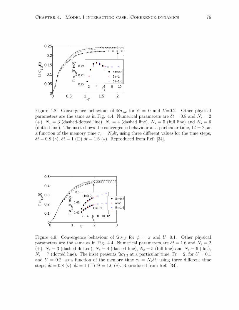
Chapter 4. Model I interacting case: Coherence dynamics 76
0 0.5 1 1.5 20
0.05
0.1
0.15
0.2
0.25
tΓ
ℜ σ
1,2(t
)
2 4 6 8 100.22
0.23
0.24
τc
ℜ σ
1,2(Γ
t=2)
δ t=0.8
δ t=1
δ t=1.6
Figure 4.8: Convergence behaviour of ℜσ1,2 for φ = 0 and U=0.2. Other physicalparameters are the same as in Fig. 4.4. Numerical parameters are δt = 0.8 and Ns = 2(+), Ns = 3 (dashed-dotted line), Ns = 4 (dashed line), Ns = 5 (full line) and Ns = 6(dotted line). The inset shows the convergence behaviour at a particular time, Γt = 2, asa function of the memory time τc = Nsδt, using three different values for the time steps,δt = 0.8 (◦), δt = 1 (�) δt = 1.6 (∗). Reproduced from Ref. [34].
0 1 2 30
0.1
0.2
0.3
0.4
0.5
tΓ
ℑ σ
1,2(t
)
2 4 6 8 10 120.42
0.46
0.5
τc
ℑ σ
1,2(Γ
t=2)
U=0.1
U=0.2δ t=0.8
δ t=1
δ t=1.6
Figure 4.9: Convergence behaviour of ℑσ1,2 for φ = π and U=0.1. Other physicalparameters are the same as in Fig. 4.4. Numerical parameters are δt = 1.6 and Ns = 2(+), Ns = 3 (dashed-dotted), Ns = 4 (dashed line), Ns = 5 (full line) and Ns = 6 (dot),Ns = 7 (dotted line). The inset presents ℑσ1,2 at a particular time, Γt = 2, for U = 0.1and U = 0.2, as a function of the memory time τc = Nsδt, using three different timesteps, δt = 0.8 (◦), δt = 1 (�) δt = 1.6 (∗). Reproduced from Ref. [34].
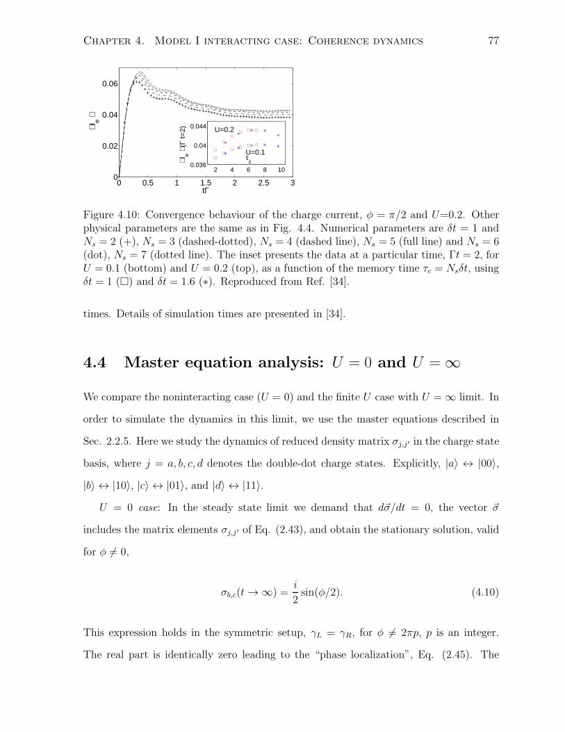
Chapter 4. Model I interacting case: Coherence dynamics 77
0 0.5 1 1.5 2 2.5 30
0.02
0.04
0.06
tΓ
⟨ Ie ⟩
2 4 6 8 100.036
0.04
0.044
τc⟨ I
e ⟩ (Γ
t=2)
U=0.1
U=0.2
Figure 4.10: Convergence behaviour of the charge current, φ = π/2 and U=0.2. Otherphysical parameters are the same as in Fig. 4.4. Numerical parameters are δt = 1 andNs = 2 (+), Ns = 3 (dashed-dotted), Ns = 4 (dashed line), Ns = 5 (full line) and Ns = 6(dot), Ns = 7 (dotted line). The inset presents the data at a particular time, Γt = 2, forU = 0.1 (bottom) and U = 0.2 (top), as a function of the memory time τc = Nsδt, usingδt = 1 (�) and δt = 1.6 (∗). Reproduced from Ref. [34].
times. Details of simulation times are presented in [34].
4.4 Master equation analysis: U = 0 and U = ∞
We compare the noninteracting case (U = 0) and the finite U case with U = ∞ limit. In
order to simulate the dynamics in this limit, we use the master equations described in
Sec. 2.2.5. Here we study the dynamics of reduced density matrix σj,j′ in the charge state
basis, where j = a, b, c, d denotes the double-dot charge states. Explicitly, |a〉 ↔ |00〉,
|b〉 ↔ |10〉, |c〉 ↔ |01〉, and |d〉 ↔ |11〉.
U = 0 case: In the steady state limit we demand that d~σ/dt = 0, the vector ~σ
includes the matrix elements σj,j′ of Eq. (2.43), and obtain the stationary solution, valid
for φ 6= 0,
σb,c(t → ∞) =i
2sin(φ/2). (4.10)
This expression holds in the symmetric setup, γL = γR, for φ 6= 2πp, p is an integer.
The real part is identically zero leading to the “phase localization”, Eq. (2.45). The
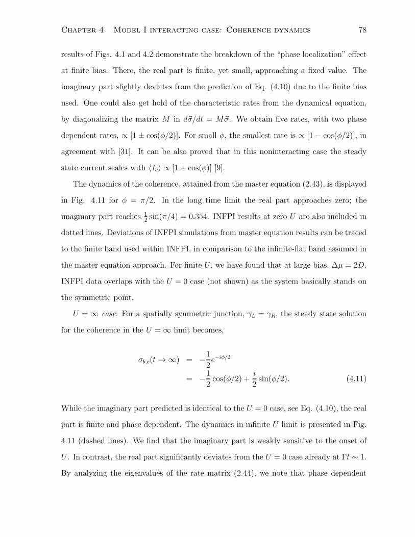
Chapter 4. Model I interacting case: Coherence dynamics 78
results of Figs. 4.1 and 4.2 demonstrate the breakdown of the “phase localization” effect
at finite bias. There, the real part is finite, yet small, approaching a fixed value. The
imaginary part slightly deviates from the prediction of Eq. (4.10) due to the finite bias
used. One could also get hold of the characteristic rates from the dynamical equation,
by diagonalizing the matrix M in d~σ/dt = M~σ. We obtain five rates, with two phase
dependent rates, ∝ [1 ± cos(φ/2)]. For small φ, the smallest rate is ∝ [1 − cos(φ/2)], in
agreement with [31]. It can be also proved that in this noninteracting case the steady
state current scales with 〈Ie〉 ∝ [1 + cos(φ)] [9].
The dynamics of the coherence, attained from the master equation (2.43), is displayed
in Fig. 4.11 for φ = π/2. In the long time limit the real part approaches zero; the
imaginary part reaches 12sin(π/4) = 0.354. INFPI results at zero U are also included in
dotted lines. Deviations of INFPI simulations from master equation results can be traced
to the finite band used within INFPI, in comparison to the infinite-flat band assumed in
the master equation approach. For finite U , we have found that at large bias, ∆µ = 2D,
INFPI data overlaps with the U = 0 case (not shown) as the system basically stands on
the symmetric point.
U = ∞ case: For a spatially symmetric junction, γL = γR, the steady state solution
for the coherence in the U = ∞ limit becomes,
σb,c(t → ∞) = −1
2e−iφ/2
= −1
2cos(φ/2) +
i
2sin(φ/2). (4.11)
While the imaginary part predicted is identical to the U = 0 case, see Eq. (4.10), the real
part is finite and phase dependent. The dynamics in infinite U limit is presented in Fig.
4.11 (dashed lines). We find that the imaginary part is weakly sensitive to the onset of
U . In contrast, the real part significantly deviates from the U = 0 case already at Γt ∼ 1.
By analyzing the eigenvalues of the rate matrix (2.44), we note that phase dependent
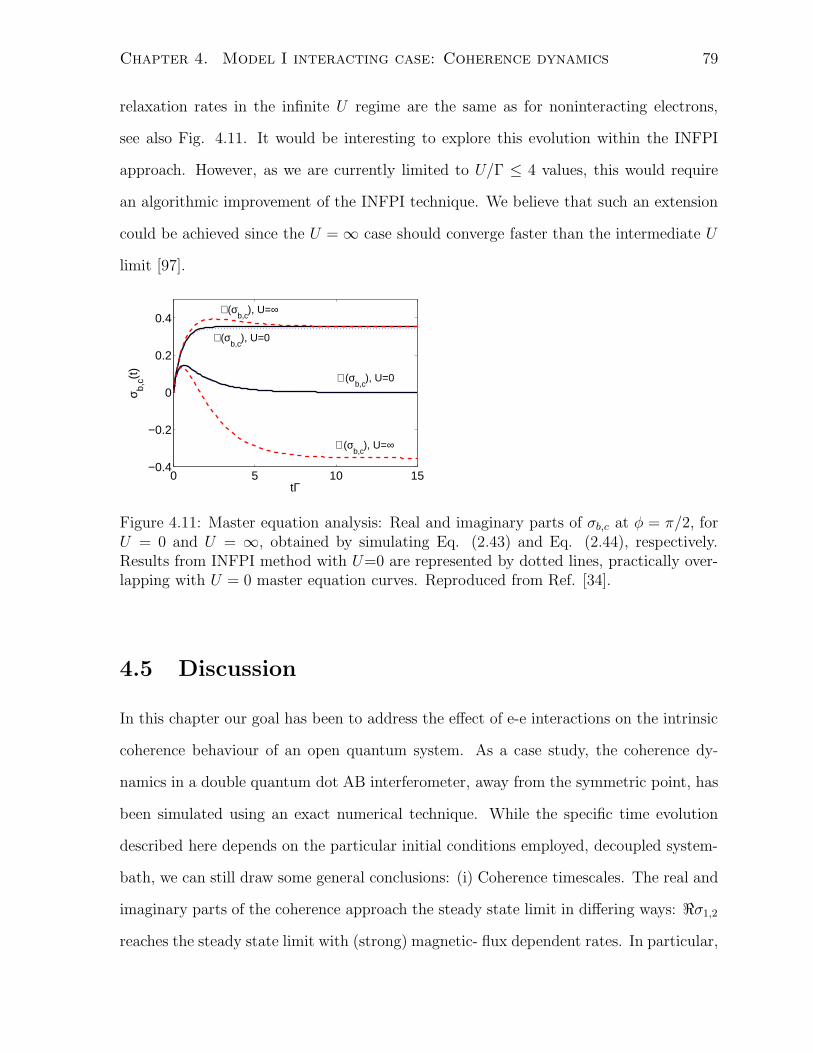
Chapter 4. Model I interacting case: Coherence dynamics 79
relaxation rates in the infinite U regime are the same as for noninteracting electrons,
see also Fig. 4.11. It would be interesting to explore this evolution within the INFPI
approach. However, as we are currently limited to U/Γ ≤ 4 values, this would require
an algorithmic improvement of the INFPI technique. We believe that such an extension
could be achieved since the U = ∞ case should converge faster than the intermediate U
limit [97].
0 5 10 15−0.4
−0.2
0
0.2
0.4
tΓ
σ b,c(t
)
ℜ (σb,c
), U=0
ℜ (σb,c
), U=∞
ℑ (σb,c
), U=0
ℑ (σb,c
), U=∞
Figure 4.11: Master equation analysis: Real and imaginary parts of σb,c at φ = π/2, forU = 0 and U = ∞, obtained by simulating Eq. (2.43) and Eq. (2.44), respectively.Results from INFPI method with U=0 are represented by dotted lines, practically over-lapping with U = 0 master equation curves. Reproduced from Ref. [34].
4.5 Discussion
In this chapter our goal has been to address the effect of e-e interactions on the intrinsic
coherence behaviour of an open quantum system. As a case study, the coherence dy-
namics in a double quantum dot AB interferometer, away from the symmetric point, has
been simulated using an exact numerical technique. While the specific time evolution
described here depends on the particular initial conditions employed, decoupled system-
bath, we can still draw some general conclusions: (i) Coherence timescales. The real and
imaginary parts of the coherence approach the steady state limit in differing ways: ℜσ1,2
reaches the steady state limit with (strong) magnetic- flux dependent rates. In particular,
Chapter 4. Model I interacting case: Coherence dynamics 80
the timescale to reach the asymptotic limit is very slow for small φ. In contrast, ℑσ1,2
approaches steady state within a time scale that is flux-independent. This observation
is valid away from the symmetric point, at finite interaction strengths and at low or
high temperatures. (ii) Transport properties and subsystem dynamics. Comparing the
time evolution of the coherences in Figs. 4.1 and 4.4 to the evolution of the current as
depicted in Fig. 4.7, we note that the charge current approaches steady state around
Γt ∼ 2 (βν = 200), in a phase independent rate, similarly to the behaviour of ℑσ1,2. It
can be also shown, at least at the symmetric point, that the double-dot occupancy is
proportional to ℜσ1,2 in the asymptotic long-time limit [31]. These relations suggest that
the current dynamics, or more generally, transport coefficients, connect to the dynamics
concealed within ℑσ1,2. The dot occupation, an impurity property, correlates in some
limit with ℜσ1,2. Understanding the correspondence between transport properties, e.g.,
current, current noise, Seebeck coefficient, and impurity properties such as population
and coherences, is a topic of fundamental interest in nonequilibrium open quantum sys-
tems [95]. Our results here demonstrate a nontrivial connection between the current and
ℑσ1,2. It is of interest to further explore these relations analytically.
More particular observations include the following points: (i) Coherence symmetry,
with respect to the magnetic flux, observed at U = 0 and at low temperatures, is main-
tained even when e-e interactions are turned on, and at high temperatures. (ii) The
charge current displays the effect of perfect destructive interference in the long time limit
for φ = π, irrespective of the onset of e-e interactions, see Fig. 4.7, indicating that “phase
rigidity” is obeyed in symmetric and degenerate double-dot interferometer beyond linear
regime even with many-body interactions. While temporal characteristics are sensitive
to the actual U -value employed, the different curves concurrently merge around tΓ ∼ 1.
(iii) At finite interactions, U/Γ ≤ 4, at low or high temperatures, we have found that the
coherence evolves similarly to the U = 0 case, showing related characteristic timescales
and long time values. Specifically, for φ = π/2 the real part of σ1,2 approaches a small
Chapter 4. Model I interacting case: Coherence dynamics 81
number (zero at the symmetric point), while the imaginary part is larger, ∼ 0.35. On the
other hand, a master equation treatment in the infinite U regime predicts a significantly
different behaviour: The magnitude of ℜσ1,2 and ℑσ1,2 should be the same,√2/4, for
the φ = π/2 phase factor.
We have discussed so far only coherent dynamics in double-dot AB interferometer.
It is interesting to study how phase breaking processes affect phase rigidity. In the next
chapter we include quasi-elastic dephasing effects by means of Buttiker dephasing probes
using nonequilibrium Green’s functions. We also discuss the role of inelastic scattering
and capacitive coupling to equilibrium and nonequilibrium environments.
Chapter 5
Symmetries of nonlinear transport
5.1 Introduction
In previous chapters we studied the dynamics of the reduced density matrix and the
charge current in interacting systems using different techniques: a numerically exact
influence functional path integral method, master equations valid in the infinite U limit.
We also discussed magnetic flux control of dot occupations with and without elastic
dephasing effects, using a probe. In this chapter we focus on magnetic field symmetries
of nonlinear transport coefficients in the presence of many body effects, taken into account
by a phenomenological technique, the probe reservoir, discussed in chapter 2.
Our objective here is to provide a systematic and comprehensive analysis of the role
of different types of probes on transport symmetries in nonlinear conductors. We want to
understand the role of elastic dephasing, heat dissipation, and charge leakage processes on
symmetries of charge current, rectification, and heat current in two-terminal conductors,
with respect to the magnetic field, temperature bias, and voltage bias. Specifically, our
main goal is to develop, and analyze the breakdown, of magnetic field symmetry relations
for nonlinear transport beyond the Onsager-Casimir result in the presence of incoherent
82
Chapter 5. Symmetries of nonlinear transport 83
effects. Expanding the charge current in powers of the bias ∆µ we write [162]
I(φ) = G1(φ)∆µ+G2(φ)(∆µ)2 +G3(φ)(∆µ)3 + ... (5.1)
with Gn>1 as the nonlinear conductance coefficients. We incorporate many body effects
using Buttiker probes. (i) We confirm the validity of Onsager-Casimir symmetry of
linear conductance (G1(φ) = G1(−φ)) using an approach based on quantum mechanical
equations of motion while allowing for elastic and inelastic effects. (ii) We obain magnetic
field symmetries and magnetoasymmetries of higher order conductance coefficients.
Our study of transport behaviour beyond linear response further exposes sufficient
conditions for the onset of the charge current rectification (diode) effect, referring to the
situation where the magnitude of the current differs when the bias polarity is reversed.
This effect, of fundamental and practical interest, is realized by combining many body
interactions with a broken symmetry: broken spatial inversion symmetry or a broken
time reversal symmetry. Rectifiers of the first type have been extensively investigated
theoretically and experimentally, including electronic rectifiers, thermal rectifiers [44] and
acoustic rectifiers [126]. In parallel, optical and spin rectifiers were designed based on a
broken time reversal symmetry, recently realized e.g. by engineering parity-time meta-
materials [127]. The model system investigated in this work, a double-dot AB junction,
offers a feasible setup for devising broken time reversal rectifiers.
We consider here four different probes (dephasing, voltage, temperature and voltage-
temperature) and demonstrate with numerical simulations a stable solution and a facile
convergence for the probe parameters far from equilibrium. We discuss the operation
of the double-dot interferometer, susceptible to inelastic effects, as a charge rectifier,
when time reversal symmetry is broken. We derive symmetry relations for nonlinear
heat transfer in the presence of charge leakage. This chapter is organized as follows.
In Sec. 5.2 we introduce the main observables of interest and summarize our principal
Chapter 5. Symmetries of nonlinear transport 84
results. In Sec. 5.3 we discuss situations that fulfill phase rigidity. Magnetic field
symmetry relations in a spatially symmetric setup are derived in Sec. 5.4. Magnetic
field- gate voltage symmetries, valid for generic double-dot AB interferometer models,
are presented in Sec. 5.5. Supporting numerical simulations are included in Sec. 5.6. In
Sec. 5.7 we discuss relation of our results to other treatments. In Sec. 5.8 we present
all the conclusions. The words “diode” and “rectifier” are used interchangeably in this
work, referring to a dc-rectifier.
5.2 Symmetry measures and main results
In the main body of this chapter we restrict ourselves to voltage-biased junctions, µL 6=
µR, while setting Ta = β−1a = TL = TR. We also limit our focus to charge conserving
systems satisfying
I(φ) ≡ IL(φ) = −IR(φ), (5.2)
and study the role of elastic dephasing (dephasing probe) and dissipative (voltage probe)
and non-dissipative (voltage-temperature probe) inelastic effects on the charge trans-
port symmetries with magnetic flux. We complement this analysis by considering a
temperature-biased heat-conserving junction, TL 6= TR, µa = µL = µR and QL = −QR.
We then study the phase symmetry of the heat current, allowing for charge leakage in
the probe. We do not study the thermoelectric effect in this work.
We now define several measures for quantifying phase symmetry in a voltage-biased
three-terminal junction satisfying Eq. (5.2). In this work we study relations between two
quantities: a measure for the magnetic field asymmetry
∆I(φ) ≡ 1
2[I(φ)− I(−φ)], (5.3)
Chapter 5. Symmetries of nonlinear transport 85
and the dc-rectification current,
R(φ) ≡ 1
2[I(φ) + I(φ)]
= G2(φ)(∆µ)2 +G4(φ)(∆µ)4 + ... (5.4)
with I defined as the current obtained upon interchanging the chemical potentials of the
two terminals. We also study the behaviour of odd conductance terms,
D(φ) ≡ 1
2[I(φ)− I(φ)]
= G1(φ)∆µ+G3(φ)(∆µ)3 + ... (5.5)
For a non-interacting system we expect the relation
I(φ) = −I(−φ) (5.6)
to hold. Combined with Eq. (5.1) we immediately note that G2n+1(φ) = G2n+1(−φ) and
G2n(φ) = −G2n(−φ) with n as an integer. We show below that these relations are obeyed
in a symmetric junction even when many body interactions (inelastic scattering) are
included. This result is not trivial since the included many body interactions are reflected
by probe parameters which depend on the applied bias in a nonlinear manner and the
magnetic phase in an asymmetric form, thus, we cannot assume Eq. (5.6) to immediately
hold. Our analysis below relies on two basic relations. First, the transmission coefficient
from the ξ to the ν reservoir obeys reciprocity, given the unitarity and time reversal
symmetry of the scattering matrix,
Tξ,ν(ω, φ) = Tν,ξ(ω,−φ). (5.7)
Chapter 5. Symmetries of nonlinear transport 86
Second, the total probability is conserved,
∑
ξ 6=ν
Tξ,ν(ω, φ) =∑
ξ 6=ν
Tν,ξ(ω, φ). (5.8)
Using Eq. (2.20), we express the deviation from the magnetic field symmetry as
∆I =1
2
∫
[TL,R − TR,L] (fL + fR)dω +1
2
∫
[TL,P − TP,L] fLdω
+1
2
∫
[TL,PfP (−φ)− TP,LfP (φ)] dω (5.9)
For the sake of simplicity we write Tν,ξ(ω, φ) as Tν,ξ. We use the probability conservation,
Eq. (5.8), and simplify this relation,
∆I =1
2
∫
[TL,R − TR,L] fRdω +1
2
∫
[TL,PfP (−φ)− TP,LfP (φ)] dω. (5.10)
Since IL = −IR, the rectification current can be written in two equivalent forms,
R =1
2
∫
TP,L(fL + fR − fP (φ)− fP (φ))dω
= −1
2
∫
TP,R(fL + fR − fP (φ)− fP (φ))dω, (5.11)
with fP as the probe distribution when the biases µL and µR are interchanged. We can
also weight these expressions and adopt a symmetric definition
R =
∫ TP,L − TP,R
4(fL + fR − fP (φ)− fP (φ))dω (5.12)
The behaviour of odd conductance terms can be similarly written as
D(φ) =1
2
∫
{
[TL,R + TL,P + TR,L] (fL − fR)− TP,L[fP (φ)− fP (φ)]}
dω
= −1
2
∫
{
[TL,R + TR,P + TR,L] (fR − fL)− TP,R[fP (φ)− fP (φ)]}
dω (5.13)
Chapter 5. Symmetries of nonlinear transport 87
Our results are organized by systematically departing from quantum coherent scenar-
ios, the linear response regime, and spatially symmetric situations. This chapter includes
four parts, and we now summarize our main results:
(i) Phase Rigidity. In Sec. 5.3 we discuss two scenarios that do obey the Onsager-
Casimir symmetry relation I(φ)=I(−φ): It is maintained in the presence of elastic de-
phasing effects even beyond linear response. This relation is also valid when inelastic
scatterings are included, albeit only in the linear response regime. While these results
are not new [64], we include this analysis here so as to clarify the role of inelastic effects
in breaking the Onsager symmetry, beyond linear response.
(ii) Magnetic field (MF) symmetry relations beyond linear response. In Sec. 5.4
we derive magnetic-field symmetry relations that hold beyond linear response in spa-
tially symmetric junctions susceptible to inelastic effects, R(φ) = ∆I(φ) = −R(−φ) and
D(φ) = D(−φ). In other words, we show that odd (even) conductance terms are even
(odd) in the magnetic flux. Note that “spatial” or “geometrical” symmetry refers here
to the left-right mirror symmetry of the junction. Below we refer to these symmetries as
the “MF symmetry relations” .
(iii) Magnetic field-Gate voltage (MFGV) symmetry relations beyond linear response.
In Secs. 5.5-5.6 we focus on geometrically asymmetric setups, adopting the double dot AB
interferometer as an example. While we demonstrate, using numerical simulations, the
breakdown of the MF relations under spatial asymmetry, we prove that charge conjuga-
tion symmetry entails magnetic field-gate voltage symmetries: R(ǫd, φ) = −R(−ǫd,−φ),
and D(−ǫd,−φ) = D(ǫd, φ), with ǫd as the double-dot energies. We refer below to these
symmetries as the “MFGV symmetry relations” .
(iv) we also prove that the heat current (within a heat-conserving setup) satisfies
relations analogous to (i)-(iii).
Chapter 5. Symmetries of nonlinear transport 88
5.3 Phase rigidity and absence of rectification
In this section we adopt a formalism based on quantum mechanical equations of motion
and demonstrate that, consistent with the theory of irreversible thermodynamics: (i) The
symmetry I(φ) = I(−φ) is preserved under quasi-elastic dephasing effects, implemented
via a dephasing probe (ii) Onsager-Casimir symmetry is obeyed in the presence of inelastic
effects implemented using the voltage probe technique. These results have already been
discussed in e.g., Ref. [64]. We detail these steps here so as to provide closed expressions
for the probe parameters in the linear response regime. We also show that the quasi-
elastic dephasing does not lead to diode behaviour.
5.3.1 Dephasing effects beyond linear response
Implementing the dephasing probe (2.23) we obtain the respective distribution
fP (φ) =TL,PfL + TR,PfR
TP,L + TP,R. (5.14)
We substitute this function into Eq. (5.10), the measure for phase asymmetry, and obtain
∆I =1
2
∫
[TL,R − TR,L] fRdω +1
2
∫
TL,PTP,LfL + TP,RfRTL,P + TR,P
dω
− 1
2
∫
TP,LTL,PfL + TR,PfR
TP,L + TP,Rdω (5.15)
The denominators in these integrals are identical, see Eq. (5.8), thus we combine the last
two terms into
∆I =1
2
∫
[TL,R − TR,L] fRdω +1
2
∫
[TL,PTP,R − TP,LTR,P ] fRTP,R + TP,L
dω. (5.16)
Chapter 5. Symmetries of nonlinear transport 89
Utilizing Eq. (5.8) in the form TL,P = TP,L + TP,R − TR,P , we organize the numerator of
the second integral, (TP,R − TR,P )(TP,R + TP,L)fR. This results in
∆I =1
2
∫
[TL,R − TR,L + TP,R − TR,P ] fRdω
=1
2
∫
fR
[
∑
ν 6=R
Tν,R −∑
ν 6=R
TR,ν
]
dω, (5.17)
which is identically zero, given Eq. (5.8). This concludes our proof that dephasing effects,
implemented via a dephasing probe, cannot break phase rigidity even in the nonlinear
regime. Following similar steps we show that elastic dephasing effects cannot bring about
the effect of charge rectification even when the junction acquires spatial asymmetries. We
substitute fP into Eq. (2.20) and obtain
IL =
∫
[FLfL − FRfR]dω (5.18)
with
FL =TL,R(TP,L + TP,R) + TL,PTP,R
(TP,L + TP,R). (5.19)
FR is defined analogously, interchanging L by R. We now note the following identities,
TL,PTP,R = [TP,L + TP,R − TR,P ]TP,R
= (TP,R − TR,P )(TP,R + TP,L) + TP,LTR,P
= (TR,L − TL,R)(TP,R + TP,L) + TP,LTR,P (5.20)
Reorganizing the first and third lines we find that
TL,R(TP,R + TP,L) + TL,PTP,R = TR,L(TP,R + TP,L) + TP,LTR,P (5.21)
Chapter 5. Symmetries of nonlinear transport 90
which immediately implies that FL = FR. This is turn leads to I = −I, thus R = 0. We
conclude that the current only includes odd (linear and nonlinear) conductance terms
under elastic dephasing, I = D(φ) = D(−φ), and that phase rigidity is maintained even
if spatial asymmetry is presented. This conclusion in valid under both applied voltage
and temperature biases.
5.3.2 Inelastic effects in linear response
We introduce inelastic effects using the voltage probe technique. In the linear response
regime we expand the Fermi functions of the three terminals around the equilibrium state
fa(ω) = [eβa(ω−µa) + 1]−1,
fν(ω) = fa(ω)− (µν − µa)∂fa∂ω
. (5.22)
The three terminals are maintained at the same temperature Ta. The derivative ∂fa∂ω
is
evaluated at the equilibrium value µa. For simplicity we set µa = 0. We enforce the
voltage probe condition, IP = 0, demanding that
∫
[(TP,L + TP,R) fP (φ)− TL,PfL − TR,PfR] dω = 0. (5.23)
In linear response this translates to
0 =
∫
[
(TP,L + TP,R)
(
fa − µP (φ)∂fa∂ω
)
− TL,P
(
fa − µL∂fa∂ω
)
− TR,P
(
fa − µR∂fa∂ω
)
]
dω. (5.24)
Chapter 5. Symmetries of nonlinear transport 91
For convenience, we apply the voltage in a symmetric manner, µL = −µR = ∆µ/2. We
organize Eq. (5.24) and obtain the probe chemical potential, a linear function in ∆µ,
µP (φ) =∆µ
2
∫
dω ∂fa∂ω
(TL,P − TR,P )∫
dω ∂fa∂ω
(TP,L + TP,R). (5.25)
We simplify this result by introducing a short notation for the conductance between the
ν and ξ terminals,
Gν,ξ(φ) ≡∫
dω
(
−∂fa∂ω
)
Tν,ξ(ω, φ). (5.26)
This quantity fulfills relations analogous to Eqs. (5.7) and (5.8). For brevity, we do
not write next the phase variable in G, evaluating it at the phase φ unless otherwise
mentioned. The probe potential can now be compacted,
µP (φ) =∆µ
2
GL,P −GR,P
GP,L +GP,R. (5.27)
Furthermore, in geometrically symmetric systems TR,P (ω, φ) = TP,L(ω, φ), resulting in
GR,P (φ) = GP,L(φ) and
µP (φ) =∆µ
2
GL,P (φ)−GL,P (−φ)
GL,P (φ) +GL,P (−φ). (5.28)
Thus µP (φ) = −µP (−φ) in linear response. Below we show that this symmetry does not
hold far from equilibrium. We now expand Eq. (5.10) in the linear response regime
∆I =1
2
∫
(TL,R − TR,L)
(
fa − µR∂fa∂ω
)
dω
+1
2
∫
{
TL,P
[
fa − µP (−φ)∂fa∂ω
]
− TP,L
[
fa − µP (φ)∂fa∂ω
]
}
dω. (5.29)
Chapter 5. Symmetries of nonlinear transport 92
Utilizing the definition (5.26) we compact this expression,
∆I =1
2(GL,R −GR,L)µR
− 1
2[GP,LµP (φ)−GL,PµP (−φ)] . (5.30)
Using Eq. (5.8), the first line can be rewritten as
I1 =∆µ
4(GL,P −GP,L) . (5.31)
The second line in Eq. (5.30) reduces to
I2 = −∆µ
4GP,L
GL,P −GR,P
N +∆µ
4GL,P
GP,L −GP,R
N= −∆µ
4
GL,PGP,R −GP,LGR,P
N (5.32)
where we have introduced the short notation N ≡ GP,L + GP,R. Now, we substitute
GL,P = GP,L +GP,R −GR,P , and this allows us to write
I2 = −∆µ
4
(GP,R −GR,P )(GP,R +GP,L)
N= −∆µ
4(GP,R −GR,P ). (5.33)
Combining ∆I = I1 + I2, we reach
∆I = −∆µ
4(GP,R −GR,P −GL,P +GP,L)
= −∆µ
4
(
∑
ν 6=P
GP,ν −∑
ν 6=P
Gν,P
)
(5.34)
which is identically zero given the conductance conservation (5.8). It is trivial to note
that no rectification takes place in the linear response regime, R = 0.
Chapter 5. Symmetries of nonlinear transport 93
5.4 Beyond linear response: spatially symmetric se-
tups
In this section we consider the role of inelastic effects on the current symmetry in an AB
interferometer, beyond the linear response regime. The probe condition IP = 0 translates
Eq. (2.21) into three relations,
∫
dω(TP,L + TP,R)fP (φ) =
∫
dω(TL,PfL + TR,PfR)∫
dω(TL,P + TR,P )fP (−φ) =
∫
dω(TP,LfL + TP,RfR)∫
dω(TP,L + TP,R)fP (φ) =
∫
dω (TL,PfR + TR,PfL) . (5.35)
First, we consider the situation when time reversal symmetry is protected, with the
magnetic phase given by multiples of 2π. Then, Tν,ξ = Tξ,ν , and particularly we note
that TL,P = TP,L. Furthermore, in the model considered in Sec. 5.5, TP,L = χTP,R, with
χ as an energy independent parameter, reflecting spatial asymmetry, see for example the
discussion around Eq. (5.45). Using the voltage probe condition (5.35) we find that
∫
(TP,L + TP,R)(fP (φ) + fP (φ))dω =
∫
(TP,L + TP,R)(fL + fR)dω, (5.36)
Given the linear relation between TL,P and TR,P , this equality holds separately for each
transmission function,
∫
TP,ν(fP (φ) + fP (φ))dω =
∫
TP,ν(fL + fR)dω ν = L,R, (5.37)
providing R = 0 in Eq. (5.12). Thus, if TP,L = TL,P = χTP,R, rectification is absent. In
physical terms, the junction conducts symmetrically for forward and reversed direction,
though many body effects are presented, if we satisfy two conditions: (i) Spatial asymme-
try is included in an energy-independent manner, for example using different broad-band
Chapter 5. Symmetries of nonlinear transport 94
hybridization parameters at the two ends. (ii) Time reversal symmetry is protected.
We now derive symmetry relations for left-right symmetric systems with broken time-
reversal symmetry. In this case the mirror symmetry TP,L(φ) = TP,R(−φ) applies, trans-
lating to
TP,L(φ) = TR,P (φ). (5.38)
When used in Eq. (5.35), we note that the distributions should obey
fP (φ) = fP (−φ), (5.39)
leading to µP (φ) = µP (−φ). We emphasize that µP (φ) itself does not posses a phase
symmetry.
Since the leakage of charge into the probe is prohibited, the deviation from phase
rigidity, Eq. (5.10), can be also expressed in terms of the current IR, to provide (note
the sign convention)
∆I(φ) =1
2
∫
dω[(TL,R − TR,L)fL − TR,PfP (−φ) + TP,RfP (φ)]. (5.40)
We define ∆I by the average of Eqs. (5.10) and (5.40),
∆I(φ) =1
4
∫
dω[
(TL,R − TR,L)(fL + fR) + (TL,P − TR,P )fP (−φ) + (TP,R − TP,L)fP (φ)]
.
We proceed and make use of two relations: TL,R − TR,L = TP,L − TL,P , and Eq (5.38),
valid in geometrically symmetric junctions. With this at hand we write
∆I(φ) =1
4
∫
(TP,L − TP,R)(fL + fR − fP (φ)− fP (φ))dω
= R(φ) = −R(−φ), (5.41)
Chapter 5. Symmetries of nonlinear transport 95
This concludes our derivation of the MF symmetries,
∆I(φ) = R(φ) = −R(−φ), D(φ) = D(−φ). (5.42)
In spatially symmetric systems odd conductance terms acquire even symmetry with re-
spect to the magnetic field, as noted experimentally [39, 107], while even conductance
terms, constructing R, are odd with respect to φ. This result was also obtained ana-
lytically in a two-terminal AB interferometer, when strong electron-electron interactions
were taken into account in the quantum dot, beyond the mean-field approach [113]. The
relation ∆I(φ) = R(φ) could be exploited in experimental studies: One could determine
whether a quantum dot junction is L-R symmetric by testing this equality.
We now emphasize the following points: (i) Eq. (5.42) does not hold when a spatial
asymmetry is introduced, by coupling the scattering centers unevenly to the leads. (ii)
The derivation of Eq. (5.42) does not assume a particular form for the density of states
of either the L and R leads, or the probe reservoir, as long as Eq. (5.38) is satisfied.
(iii) The symmetry relations obtained here are valid under the more restrictive (non-
dissipative) voltage-temperature probe, Eq. (2.30). (iv) The analysis in this section
reveals sufficient conditions for charge rectification for structurally symmetric junctions:
R(φ) 6= 0 when time-reversal symmetry is broken, φ 6= 2πn, and inelastic scatterings
(effective anharmonicity) are allowed.
5.5 Beyond linear response: model II
In this section we demonstrate our analytical results. We adopt a double-dot AB model
with a probe coupled to dot ’1’, see Fig. 2.2, to allow for inelastic effects. The Hamilto-
Chapter 5. Symmetries of nonlinear transport 96
nian has the following form,
H = HAB +∑
p∈Pωpa
†pap +
∑
p∈Pλpa
†1ap + h.c. (5.43)
We voltage-bias the system, ∆µ ≡ µL − µR, with µL,R as the chemical potential
of the metals, and use the convention that a positive current is flowing left-to-right.
While we bias the system in a symmetric manner, µL = −µR, this choice does not limit
the generality of our discussion since the dots may be gated away from the so called
“symmetric point” at which µL − ǫβ = ǫβ − µR.
5.5.1 Transmission functions
Our model does not include interacting particles, thus its steady-state characteristics
can be written exactly using the nonequilibrium Green’s function approach [116, 117].
In terms of the Green’s function, the transmission coefficient is defined as
Tν,ξ = Tr[ΓνG+ΓξG−], (5.44)
where the trace is performed over the states of the subsystem (dots). In our model the
matrix G+ (G− = [G+]†) takes the form
G+ =
ω − ǫ1 +i(γL+γR+γP )
2iγL2eiφ/2 + iγR
2e−iφ/2
iγL2e−iφ/2 + iγR
2eiφ/2 ω − ǫ2 +
i(γL+γR)2
−1
,
Chapter 5. Symmetries of nonlinear transport 97
with the hybridization matrices satisfying
ΓL = γL
1 eiφ/2
e−iφ/2 1
, ΓR = γR
1 e−iφ/2
eiφ/2 1
ΓP = γP
1 0
0 0
(5.45)
The coupling energy between the dots and leads is given by
γν(ǫ) = 2π∑
j∈ν|vj|2δ(ω − ωj). (5.46)
In the wide-band limit adopted in this work γν are taken as energy independent param-
eters. We now assume that the dots are energy-degenerate, ǫd ≡ ǫ1 = ǫ2, but allow for a
spatial asymmetry in the form γL 6= γR. The transmission functions are given by
TL,R(ω, φ) =γLγR
∆(ω, φ)
[
4(ω − ǫd)2 cos2
φ
2+
γ2P
4+ γP (ǫd − ω) sinφ
]
TL,P (ω, φ) =γLγP
∆(ω, φ)
[
(ω − ǫd)2 + γ2
R sin2 φ
2+ γR(ω − ǫd) sinφ
]
TR,P (ω, φ) =γRγP
∆(ω, φ)
[
(ω − ǫd)2 + γ2
L sin2 φ
2− γL(ω − ǫd) sinφ
]
(5.47)
with the denominator an even function of φ,
∆(ω, φ) =
[
(ω − ǫd)2 − γLγR sin2 φ
2− (γL + γR)γP
4
]2
+(
γL + γR +γP2
)2
(ω − ǫd)2. (5.48)
Chapter 5. Symmetries of nonlinear transport 98
It is trivial to confirm that in the absence of the probe, an even symmetry of the current
with φ is satisfied, beyond linear response [27].
IL(φ) =
∫
dω4γLγR(ω − ǫd)
2 cos2 φ2[fL(ω)− fR(ω)]
[
(ω − ǫd)2 − γLγR sin2 φ2
]2+ (γL + γR)2(ω − ǫd)2
With the probe, inspecting the transmission functions in conjunction with Eq. (5.27),
we immediately conclude that under spatial asymmetries the probe chemical potential
does not obey a particular symmetry, even in linear response when phase rigidity is
trivially obeyed, see Sec. 5.3.2. We now discuss the properties of the probe when the
interferometer is L-R symmetric, γ/2 = γL = γR. The transmission functions satisfy
TR,P (ω, φ) = TP,L(ω, φ). We substitute these expressions into Eq. (5.14) and resolve the
distribution of a dephasing probe [115].
fDP (ω, φ) =
fL(ω) + fR(ω)
2+
γ(ω − ǫd) sinφ
4[
(ω − ǫd)2 + ω20
] [fL(ω)− fR(ω)] (5.49)
with ω0 = γ2sin φ
2. The nonequilibrium term in this distribution is odd in the magnetic
flux. Similarly, when a voltage probe (V ) is implemented, analytic results can be obtained
in the linear response regime,
µVP (φ) = ∆µ sinφ
∫
dω ∂fa∂ω
γ(ω−ǫd)∆(ω,φ)
∫
dω ∂fa∂ω
2(ω−ǫd)2+12γ2 sin2 φ
2
∆(ω,φ)
. (5.50)
Here fa stands for the equilibrium (zero bias) Fermi-Dirac function. This chemical po-
tential is an odd function of the magnetic flux, though phase rigidity is maintained in the
linear response regime.
Chapter 5. Symmetries of nonlinear transport 99
5.5.2 Generalized magnetic field-gate voltage symmetries
The MF symmetry relations (5.42) are not respected when the spatial mirror symme-
try is broken. Instead, in Sec 5.6.5 we prove that in a generic model for a double-dot
interferometer susceptible to inelastic effects the following result holds
R = −C(R), D = C(D). (5.51)
Here C stands for the charge conjugation operator, transforming electrons to holes and
vise versa. In terms of the parameters of our AB interferometer model, this relation
reduces to the following magnetic flux-gate voltage (MFGV) symmetries,
R(ǫd, φ) = −R(−ǫd,−φ),
D(ǫd, φ) = D(−ǫd,−φ). (5.52)
Since the energies of the dots can be modulated with a gate voltage [109], these general-
ized symmetries can be examined experimentally.
5.6 Numerical simulations
Using numerical simulations we demonstrate the behaviour of the voltage and the voltage-
temperature probes far from equilibrium, and the implications on phase rigidity and
magnetic field symmetries.
5.6.1 Probe parameters
We consider the model Eq. (2.1) and implement inelastic effects with the dissipative
voltage probe, by solving the probe condition (2.25) numerically-iteratively, using Eq.
(2.27), to obtain µP . We also investigate the transport behaviour of the model under
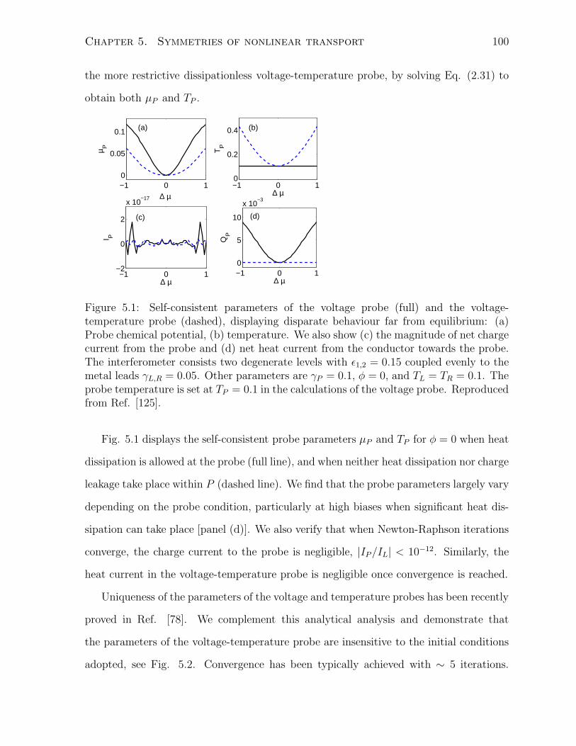
Chapter 5. Symmetries of nonlinear transport 100
the more restrictive dissipationless voltage-temperature probe, by solving Eq. (2.31) to
obtain both µP and TP .
−1 0 10
0.05
0.1
∆ µ
µ P
(a)
−1 0 10
0.2
0.4
∆ µ
TP
(b)
−1 0 1−2
0
2
x 10−17
∆ µ
I P
(c)
−1 0 10
5
10
x 10−3
∆ µ
QP
(d)
Figure 5.1: Self-consistent parameters of the voltage probe (full) and the voltage-temperature probe (dashed), displaying disparate behaviour far from equilibrium: (a)Probe chemical potential, (b) temperature. We also show (c) the magnitude of net chargecurrent from the probe and (d) net heat current from the conductor towards the probe.The interferometer consists two degenerate levels with ǫ1,2 = 0.15 coupled evenly to themetal leads γL,R = 0.05. Other parameters are γP = 0.1, φ = 0, and TL = TR = 0.1. Theprobe temperature is set at TP = 0.1 in the calculations of the voltage probe. Reproducedfrom Ref. [125].
Fig. 5.1 displays the self-consistent probe parameters µP and TP for φ = 0 when heat
dissipation is allowed at the probe (full line), and when neither heat dissipation nor charge
leakage take place within P (dashed line). We find that the probe parameters largely vary
depending on the probe condition, particularly at high biases when significant heat dis-
sipation can take place [panel (d)]. We also verify that when Newton-Raphson iterations
converge, the charge current to the probe is negligible, |IP/IL| < 10−12. Similarly, the
heat current in the voltage-temperature probe is negligible once convergence is reached.
Uniqueness of the parameters of the voltage and temperature probes has been recently
proved in Ref. [78]. We complement this analytical analysis and demonstrate that
the parameters of the voltage-temperature probe are insensitive to the initial conditions
adopted, see Fig. 5.2. Convergence has been typically achieved with ∼ 5 iterations.
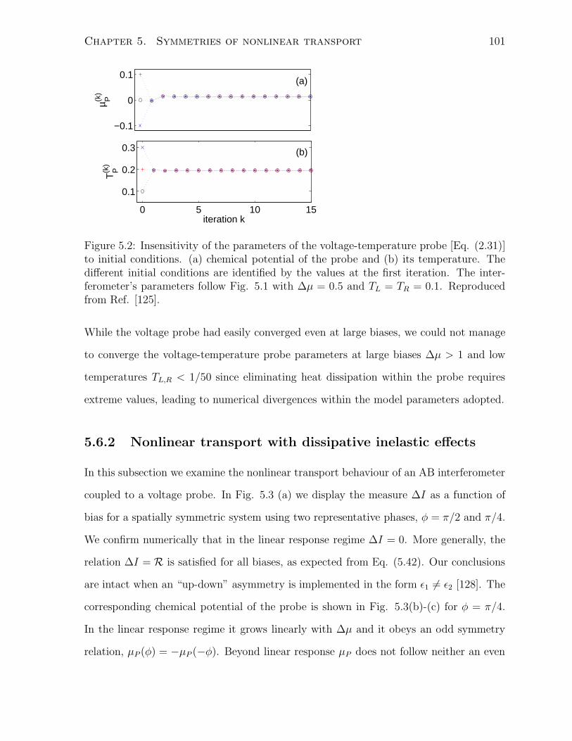
Chapter 5. Symmetries of nonlinear transport 101
−0.1
0
0.1
µ P(k)
(a)
0 5 10 15
0.1
0.2
0.3
iteration k
TP(k
)
(b)
Figure 5.2: Insensitivity of the parameters of the voltage-temperature probe [Eq. (2.31)]to initial conditions. (a) chemical potential of the probe and (b) its temperature. Thedifferent initial conditions are identified by the values at the first iteration. The inter-ferometer’s parameters follow Fig. 5.1 with ∆µ = 0.5 and TL = TR = 0.1. Reproducedfrom Ref. [125].
While the voltage probe had easily converged even at large biases, we could not manage
to converge the voltage-temperature probe parameters at large biases ∆µ > 1 and low
temperatures TL,R < 1/50 since eliminating heat dissipation within the probe requires
extreme values, leading to numerical divergences within the model parameters adopted.
5.6.2 Nonlinear transport with dissipative inelastic effects
In this subsection we examine the nonlinear transport behaviour of an AB interferometer
coupled to a voltage probe. In Fig. 5.3 (a) we display the measure ∆I as a function of
bias for a spatially symmetric system using two representative phases, φ = π/2 and π/4.
We confirm numerically that in the linear response regime ∆I = 0. More generally, the
relation ∆I = R is satisfied for all biases, as expected from Eq. (5.42). Our conclusions
are intact when an “up-down” asymmetry is implemented in the form ǫ1 6= ǫ2 [128]. The
corresponding chemical potential of the probe is shown in Fig. 5.3(b)-(c) for φ = π/4.
In the linear response regime it grows linearly with ∆µ and it obeys an odd symmetry
relation, µP (φ) = −µP (−φ). Beyond linear response µP does not follow neither an even
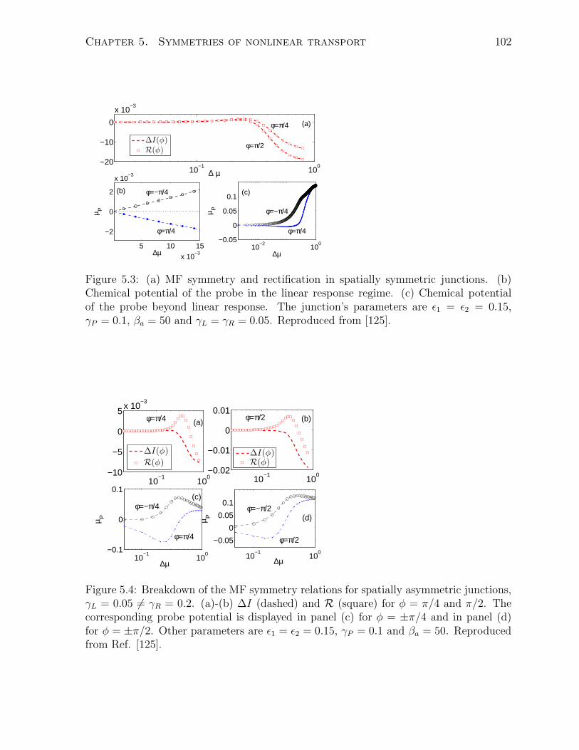
Chapter 5. Symmetries of nonlinear transport 102
10−2
100
−0.05
0
0.05
0.1
∆µ
µ P
(b)
φ=−π/4
φ=π/4
5 10 15
x 10−3
−2
0
2
x 10−3
∆µ
µ P
(c)
φ=π/4
φ=−π/4(b)
10−1
100
−20
−10
0
x 10−3
∆ µ
(a)
φ=π/2
φ=π/4
∆I(φ)R(φ)
Figure 5.3: (a) MF symmetry and rectification in spatially symmetric junctions. (b)Chemical potential of the probe in the linear response regime. (c) Chemical potentialof the probe beyond linear response. The junction’s parameters are ǫ1 = ǫ2 = 0.15,γP = 0.1, βa = 50 and γL = γR = 0.05. Reproduced from [125].
10−1
100
−0.05
0
0.05
0.1
∆µ
µ P (d)φ=−π/2
φ=π/2
10−1
100
−0.1
0
0.1
∆µ
µ P
(c)
φ=π/4
φ=−π/4
10−1
100
−0.02
−0.01
0
0.01(b)φ=π/2
10−1
100
−10
−5
0
5x 10
−3
(a)φ=π/4
∆I(φ)
R(φ)∆I(φ)R(φ)
Figure 5.4: Breakdown of the MF symmetry relations for spatially asymmetric junctions,γL = 0.05 6= γR = 0.2. (a)-(b) ∆I (dashed) and R (square) for φ = π/4 and π/2. Thecorresponding probe potential is displayed in panel (c) for φ = ±π/4 and in panel (d)for φ = ±π/2. Other parameters are ǫ1 = ǫ2 = 0.15, γP = 0.1 and βa = 50. Reproducedfrom Ref. [125].
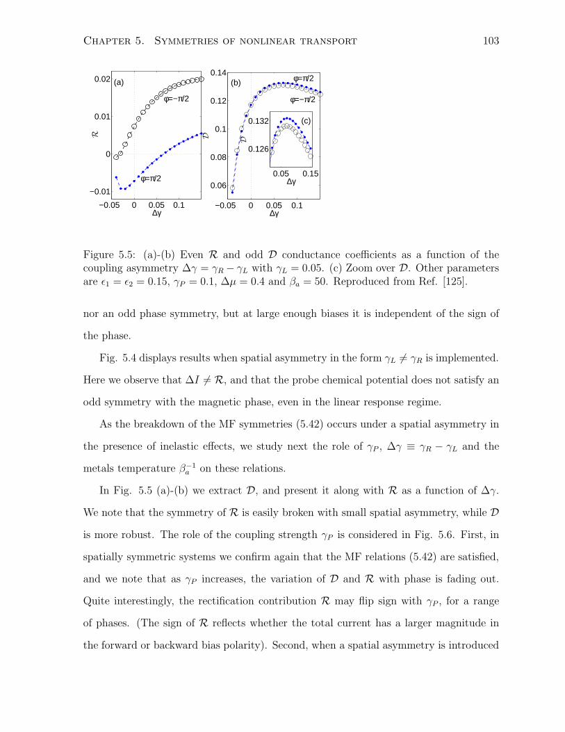
Chapter 5. Symmetries of nonlinear transport 103
−0.05 0 0.05 0.1
−0.01
0
0.01
0.02
∆γ
R
(a)
φ=−π/2
φ=π/2
−0.05 0 0.05 0.1
0.06
0.08
0.1
0.12
0.14
∆γD
(b)
φ=−π/2
φ=π/2
0.05 0.15
0.126
0.132
∆γ
D
(c)
Figure 5.5: (a)-(b) Even R and odd D conductance coefficients as a function of thecoupling asymmetry ∆γ = γR − γL with γL = 0.05. (c) Zoom over D. Other parametersare ǫ1 = ǫ2 = 0.15, γP = 0.1, ∆µ = 0.4 and βa = 50. Reproduced from Ref. [125].
nor an odd phase symmetry, but at large enough biases it is independent of the sign of
the phase.
Fig. 5.4 displays results when spatial asymmetry in the form γL 6= γR is implemented.
Here we observe that ∆I 6= R, and that the probe chemical potential does not satisfy an
odd symmetry with the magnetic phase, even in the linear response regime.
As the breakdown of the MF symmetries (5.42) occurs under a spatial asymmetry in
the presence of inelastic effects, we study next the role of γP , ∆γ ≡ γR − γL and the
metals temperature β−1a on these relations.
In Fig. 5.5 (a)-(b) we extract D, and present it along with R as a function of ∆γ.
We note that the symmetry of R is easily broken with small spatial asymmetry, while D
is more robust. The role of the coupling strength γP is considered in Fig. 5.6. First, in
spatially symmetric systems we confirm again that the MF relations (5.42) are satisfied,
and we note that as γP increases, the variation of D and R with phase is fading out.
Quite interestingly, the rectification contribution R may flip sign with γP , for a range
of phases. (The sign of R reflects whether the total current has a larger magnitude in
the forward or backward bias polarity). Second, when a spatial asymmetry is introduced
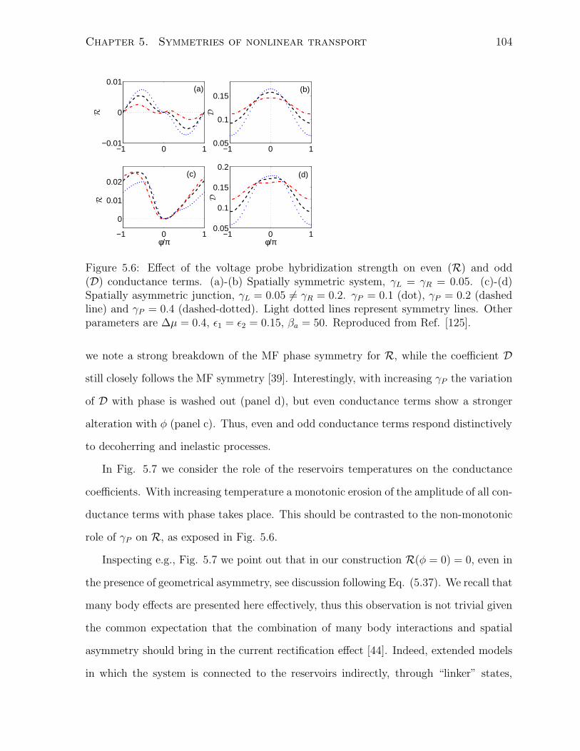
Chapter 5. Symmetries of nonlinear transport 104
−1 0 1−0.01
0
0.01
R
(a)
−1 0 10.05
0.1
0.15
D
(b)
−1 0 10.05
0.1
0.15
0.2
φ/π
D
(d)
−1 0 1
0
0.01
0.02
φ/π
R
(c)
Figure 5.6: Effect of the voltage probe hybridization strength on even (R) and odd(D) conductance terms. (a)-(b) Spatially symmetric system, γL = γR = 0.05. (c)-(d)Spatially asymmetric junction, γL = 0.05 6= γR = 0.2. γP = 0.1 (dot), γP = 0.2 (dashedline) and γP = 0.4 (dashed-dotted). Light dotted lines represent symmetry lines. Otherparameters are ∆µ = 0.4, ǫ1 = ǫ2 = 0.15, βa = 50. Reproduced from Ref. [125].
we note a strong breakdown of the MF phase symmetry for R, while the coefficient D
still closely follows the MF symmetry [39]. Interestingly, with increasing γP the variation
of D with phase is washed out (panel d), but even conductance terms show a stronger
alteration with φ (panel c). Thus, even and odd conductance terms respond distinctively
to decoherring and inelastic processes.
In Fig. 5.7 we consider the role of the reservoirs temperatures on the conductance
coefficients. With increasing temperature a monotonic erosion of the amplitude of all con-
ductance terms with phase takes place. This should be contrasted to the non-monotonic
role of γP on R, as exposed in Fig. 5.6.
Inspecting e.g., Fig. 5.7 we point out that in our construction R(φ = 0) = 0, even in
the presence of geometrical asymmetry, see discussion following Eq. (5.37). We recall that
many body effects are presented here effectively, thus this observation is not trivial given
the common expectation that the combination of many body interactions and spatial
asymmetry should bring in the current rectification effect [44]. Indeed, extended models
in which the system is connected to the reservoirs indirectly, through “linker” states,
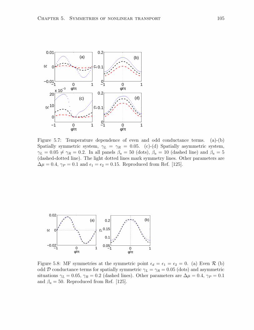
Chapter 5. Symmetries of nonlinear transport 105
−1 0 1−0.01
0
0.01
φ/π
R
(a)
−1 0 10
0.1
0.2
φ/π
D
(b)
−1 0 1
0
10
20x 10
−3
φ/π
R
(c)
−1 0 10
0.1
0.2
φ/π
D(d)
Figure 5.7: Temperature dependence of even and odd conductance terms. (a)-(b)Spatially symmetric system, γL = γR = 0.05. (c)-(d) Spatially asymmetric system,γL = 0.05 6= γR = 0.2. In all panels βa = 50 (dots), βa = 10 (dashed line) and βa = 5(dashed-dotted line). The light dotted lines mark symmetry lines. Other parameters are∆µ = 0.4, γP = 0.1 and ǫ1 = ǫ2 = 0.15. Reproduced from Ref. [125].
−1 0 1−0.02
0
0.02
φ/π
R
(a)
−1 0 10.05
0.1
0.15
0.2
φ/π
D
(b)
Figure 5.8: MF symmetries at the symmetric point ǫd = ǫ1 = ǫ2 = 0. (a) Even R (b)odd D conductance terms for spatially symmetric γL = γR = 0.05 (dots) and asymmetricsituations γL = 0.05, γR = 0.2 (dashed lines). Other parameters are ∆µ = 0.4, γP = 0.1and βa = 50. Reproduced from Ref. [125].
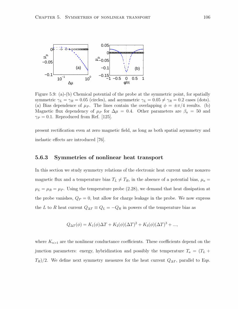
Chapter 5. Symmetries of nonlinear transport 106
−1 −0.5 0 0.5 1−0.15
−0.1
−0.05
0
0.05
φ/π
µ p
(b)
10−1
100
−0.1
−0.05
0
∆µ
µ p
(a)
Figure 5.9: (a)-(b) Chemical potential of the probe at the symmetric point, for spatiallysymmetric γL = γR = 0.05 (circles), and asymmetric γL = 0.05 6= γR = 0.2 cases (dots).(a) Bias dependence of µP . The lines contain the overlapping φ = ±π/4 results. (b)Magnetic flux dependency of µP for ∆µ = 0.4. Other parameters are βa = 50 andγP = 0.1. Reproduced from Ref. [125].
present rectification even at zero magnetic field, as long as both spatial asymmetry and
inelastic effects are introduced [76].
5.6.3 Symmetries of nonlinear heat transport
In this section we study symmetry relations of the electronic heat current under nonzero
magnetic flux and a temperature bias TL 6= TR, in the absence of a potential bias, µa =
µL = µR = µP . Using the temperature probe (2.28), we demand that heat dissipation at
the probe vanishes, QP = 0, but allow for charge leakage in the probe. We now express
the L to R heat current Q∆T ≡ QL = −QR in powers of the temperature bias as
Q∆T (φ) = K1(φ)∆T +K2(φ)(∆T )2 +K3(φ)(∆T )3 + ...,
where Kn>1 are the nonlinear conductance coefficients. These coefficients depend on the
junction parameters: energy, hybridization and possibly the temperature Ta = (TL +
TR)/2. We define next symmetry measures for the heat current Q∆T , parallel to Eqs.
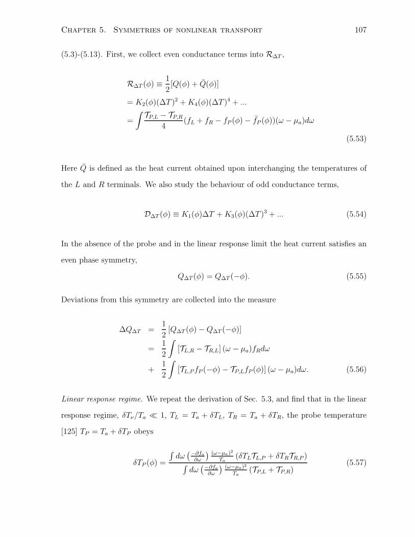
Chapter 5. Symmetries of nonlinear transport 107
(5.3)-(5.13). First, we collect even conductance terms into R∆T ,
R∆T (φ) ≡1
2[Q(φ) + Q(φ)]
= K2(φ)(∆T )2 +K4(φ)(∆T )4 + ...
=
∫ TP,L − TP,R
4(fL + fR − fP (φ)− fP (φ))(ω − µa)dω
(5.53)
Here Q is defined as the heat current obtained upon interchanging the temperatures of
the L and R terminals. We also study the behaviour of odd conductance terms,
D∆T (φ) ≡ K1(φ)∆T +K3(φ)(∆T )3 + ... (5.54)
In the absence of the probe and in the linear response limit the heat current satisfies an
even phase symmetry,
Q∆T (φ) = Q∆T (−φ). (5.55)
Deviations from this symmetry are collected into the measure
∆Q∆T =1
2[Q∆T (φ)−Q∆T (−φ)]
=1
2
∫
[TL,R − TR,L] (ω − µa)fRdω
+1
2
∫
[TL,PfP (−φ)− TP,LfP (φ)] (ω − µa)dω. (5.56)
Linear response regime. We repeat the derivation of Sec. 5.3, and find that in the linear
response regime, δTν/Ta ≪ 1, TL = Ta + δTL, TR = Ta + δTR, the probe temperature
[125] TP = Ta + δTP obeys
δTP (φ) =
∫
dω(−∂fa
∂ω
) (ω−µa)2
Ta(δTLTL,P + δTRTR,P )
∫
dω(−∂fa
∂ω
) (ω−µa)2
Ta(TP,L + TP,R)
(5.57)
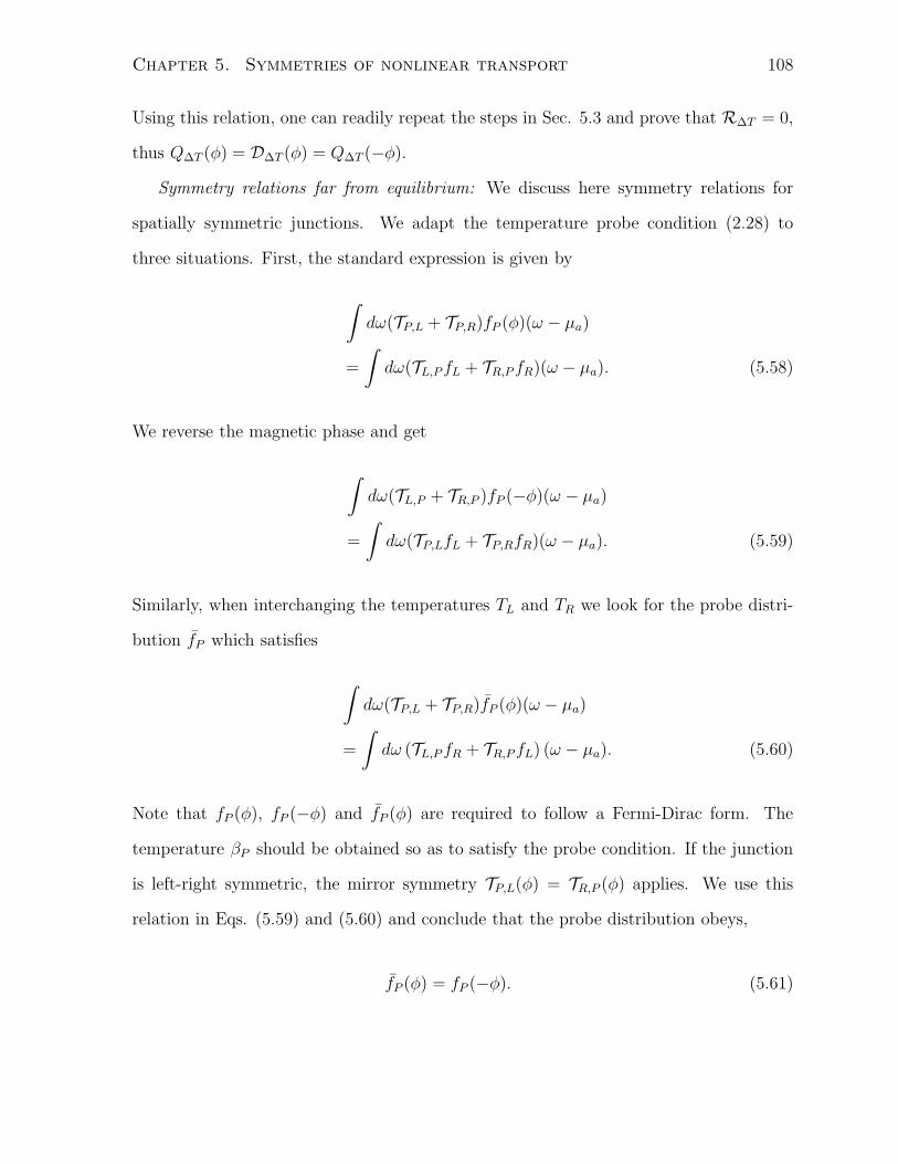
Chapter 5. Symmetries of nonlinear transport 108
Using this relation, one can readily repeat the steps in Sec. 5.3 and prove that R∆T = 0,
thus Q∆T (φ) = D∆T (φ) = Q∆T (−φ).
Symmetry relations far from equilibrium: We discuss here symmetry relations for
spatially symmetric junctions. We adapt the temperature probe condition (2.28) to
three situations. First, the standard expression is given by
∫
dω(TP,L + TP,R)fP (φ)(ω − µa)
=
∫
dω(TL,PfL + TR,PfR)(ω − µa). (5.58)
We reverse the magnetic phase and get
∫
dω(TL,P + TR,P )fP (−φ)(ω − µa)
=
∫
dω(TP,LfL + TP,RfR)(ω − µa). (5.59)
Similarly, when interchanging the temperatures TL and TR we look for the probe distri-
bution fP which satisfies
∫
dω(TP,L + TP,R)fP (φ)(ω − µa)
=
∫
dω (TL,PfR + TR,PfL) (ω − µa). (5.60)
Note that fP (φ), fP (−φ) and fP (φ) are required to follow a Fermi-Dirac form. The
temperature βP should be obtained so as to satisfy the probe condition. If the junction
is left-right symmetric, the mirror symmetry TP,L(φ) = TR,P (φ) applies. We use this
relation in Eqs. (5.59) and (5.60) and conclude that the probe distribution obeys,
fP (φ) = fP (−φ). (5.61)
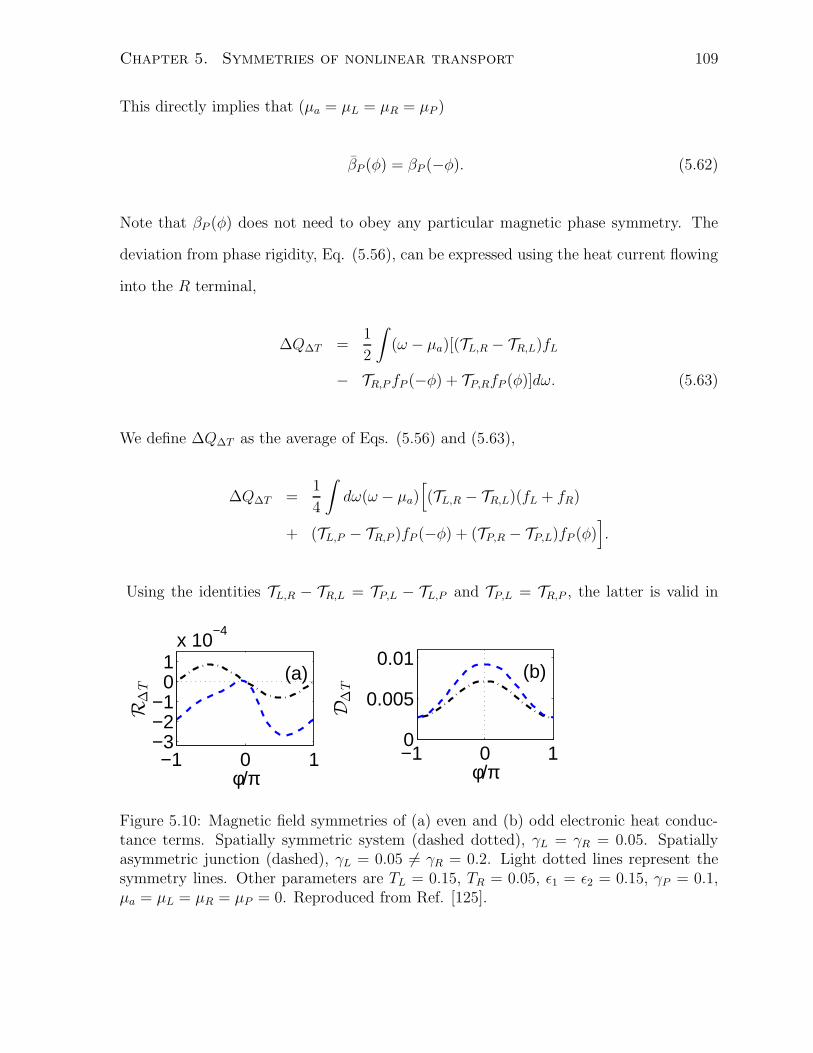
Chapter 5. Symmetries of nonlinear transport 109
This directly implies that (µa = µL = µR = µP )
βP (φ) = βP (−φ). (5.62)
Note that βP (φ) does not need to obey any particular magnetic phase symmetry. The
deviation from phase rigidity, Eq. (5.56), can be expressed using the heat current flowing
into the R terminal,
∆Q∆T =1
2
∫
(ω − µa)[(TL,R − TR,L)fL
− TR,PfP (−φ) + TP,RfP (φ)]dω. (5.63)
We define ∆Q∆T as the average of Eqs. (5.56) and (5.63),
∆Q∆T =1
4
∫
dω(ω − µa)[
(TL,R − TR,L)(fL + fR)
+ (TL,P − TR,P )fP (−φ) + (TP,R − TP,L)fP (φ)]
.
Using the identities TL,R − TR,L = TP,L − TL,P and TP,L = TR,P , the latter is valid in
−1 0 1−3−2−1
01
x 10−4
φ/π
R∆T
(a)
−1 0 10
0.005
0.01
φ/π
D∆T
(b)
Figure 5.10: Magnetic field symmetries of (a) even and (b) odd electronic heat conduc-tance terms. Spatially symmetric system (dashed dotted), γL = γR = 0.05. Spatiallyasymmetric junction (dashed), γL = 0.05 6= γR = 0.2. Light dotted lines represent thesymmetry lines. Other parameters are TL = 0.15, TR = 0.05, ǫ1 = ǫ2 = 0.15, γP = 0.1,µa = µL = µR = µP = 0. Reproduced from Ref. [125].
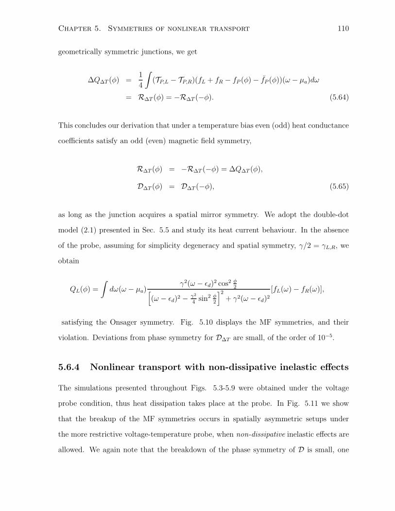
Chapter 5. Symmetries of nonlinear transport 110
geometrically symmetric junctions, we get
∆Q∆T (φ) =1
4
∫
(TP,L − TP,R)(fL + fR − fP (φ)− fP (φ))(ω − µa)dω
= R∆T (φ) = −R∆T (−φ). (5.64)
This concludes our derivation that under a temperature bias even (odd) heat conductance
coefficients satisfy an odd (even) magnetic field symmetry,
R∆T (φ) = −R∆T (−φ) = ∆Q∆T (φ),
D∆T (φ) = D∆T (−φ), (5.65)
as long as the junction acquires a spatial mirror symmetry. We adopt the double-dot
model (2.1) presented in Sec. 5.5 and study its heat current behaviour. In the absence
of the probe, assuming for simplicity degeneracy and spatial symmetry, γ/2 = γL,R, we
obtain
QL(φ) =
∫
dω(ω − µa)γ2(ω − ǫd)
2 cos2 φ2
[
(ω − ǫd)2 − γ2
4sin2 φ
2
]2
+ γ2(ω − ǫd)2[fL(ω)− fR(ω)],
satisfying the Onsager symmetry. Fig. 5.10 displays the MF symmetries, and their
violation. Deviations from phase symmetry for D∆T are small, of the order of 10−5.
5.6.4 Nonlinear transport with non-dissipative inelastic effects
The simulations presented throughout Figs. 5.3-5.9 were obtained under the voltage
probe condition, thus heat dissipation takes place at the probe. In Fig. 5.11 we show
that the breakup of the MF symmetries occurs in spatially asymmetric setups under
the more restrictive voltage-temperature probe, when non-dissipative inelastic effects are
allowed. We again note that the breakdown of the phase symmetry of D is small, one
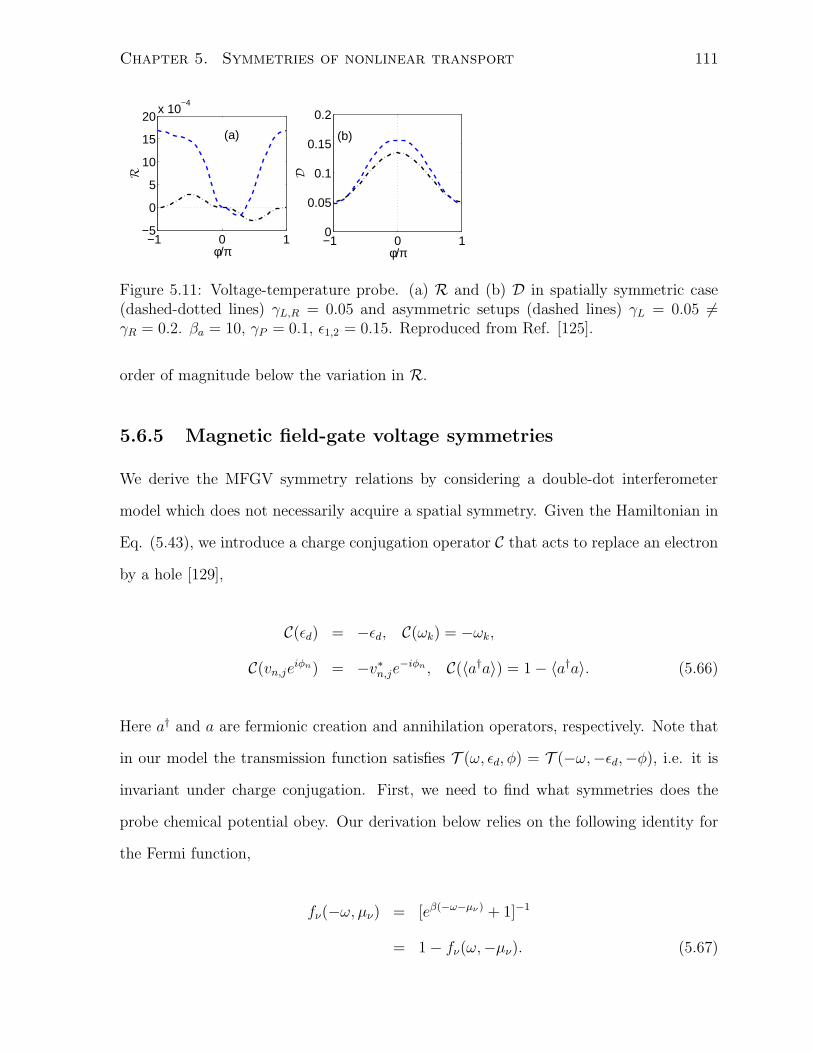
Chapter 5. Symmetries of nonlinear transport 111
−1 0 1−5
0
5
10
15
20x 10
−4
φ/π
R(a)
−1 0 10
0.05
0.1
0.15
0.2
φ/π
D
(b)
Figure 5.11: Voltage-temperature probe. (a) R and (b) D in spatially symmetric case(dashed-dotted lines) γL,R = 0.05 and asymmetric setups (dashed lines) γL = 0.05 6=γR = 0.2. βa = 10, γP = 0.1, ǫ1,2 = 0.15. Reproduced from Ref. [125].
order of magnitude below the variation in R.
5.6.5 Magnetic field-gate voltage symmetries
We derive the MFGV symmetry relations by considering a double-dot interferometer
model which does not necessarily acquire a spatial symmetry. Given the Hamiltonian in
Eq. (5.43), we introduce a charge conjugation operator C that acts to replace an electron
by a hole [129],
C(ǫd) = −ǫd, C(ωk) = −ωk,
C(vn,jeiφn) = −v∗n,je−iφn , C(〈a†a〉) = 1− 〈a†a〉. (5.66)
Here a† and a are fermionic creation and annihilation operators, respectively. Note that
in our model the transmission function satisfies T (ω, ǫd, φ) = T (−ω,−ǫd,−φ), i.e. it is
invariant under charge conjugation. First, we need to find what symmetries does the
probe chemical potential obey. Our derivation below relies on the following identity for
the Fermi function,
fν(−ω, µν) = [eβ(−ω−µν ) + 1]−1
= 1− fν(ω,−µν). (5.67)
Chapter 5. Symmetries of nonlinear transport 112
Since we use the convention µL = −µR, we conclude that fL(−ω, µL) = 1 − fR(ω, µR).
Next we omit the direct reference to the energy ω within T and the Fermi functions. Also,
we do not write the phase φ in the transmission function, unless necessary to eliminate
confusion. We now study the probe condition (5.35) as is, under reversed bias voltage,
and under charge conjugation,
∫
dω(TP,L + TP,R)fP (µP (ǫd, φ, µL, µR)) =
∫
dǫ(TL,PfL + TR,PfR) (5.68)∫
dω(TP,L + TP,R)fP (µP (ǫd, φ, µR, µL)) =
∫
dǫ (TL,PfR + TR,PfL) . (5.69)∫
dω(TP,L + TP,R)[1− fP (−µP (−ǫd,−φ, µL, µR))] =
∫
dω(TL,P [1− fR] + TR,P [1− fL])
(5.70)
For clarity, we explicitly noted the dependence of fP on the chemical potential µP , itself
obtained given the set of parameters ǫd, φ, and µL,R. Equation (5.70) now reduces to
∫
dω(TP,L + TP,R)fP (−µP (−ǫd,−φ, µL, µR))
=
∫
dω(TL,PfR + TR,PfL). (5.71)
Comparing it to Eq. (5.69) we immediately note that
fP (−µP (−ǫd,−φ, µL, µR)) = fP (µP (ǫd, φ, µR, µL)).
This result should be compared to Eq. (5.39), valid for spatially symmetric systems.
Since the three reservoirs L,R, P are maintained at the temperature Ta, this relation
implies that
µP (ǫd, φ, µL, µR) = −µP (−ǫd,−φ, µR, µL). (5.72)
Chapter 5. Symmetries of nonlinear transport 113
We now utilize Eq. (5.72) and derive symmetry relations for R and D. We recall the
explicit expressions for these measures, see the definitions (5.11) and (5.13) in Sec. 5.2.
The charge-conjugated expressions satisfy
C(R) =1
2
∫
dǫTP,L
{
[1− fR] + [1− fL]− [1− fP (−µP (−ǫd,−φ, µL, µR))]
− [1− fP (−µP (−ǫd,−φ, µR, µL)])}
= −1
2
∫
dǫTP,L {fR + fL − fP (−µP (−ǫd,−φ, µL, µR))− fP (−µP (−ǫd,−φ, µR, µL))}
= −R (5.73)
The last equality is reached by using Eq. (5.72). Similarly, we obtain the symmetry of
odd conductance terms as
C(D) =1
2
∫
dǫ{
(TL,R + TL,P + TR,L)(1− fR − 1 + fL)
− TP,L [1− fP (−µP (−ǫd,−φ, µL, µR))− 1 + fP (−µP (−ǫd,−φ, µR, µL))]}
=1
2
∫
dǫ{
(TL,R + TL,P + TR,L)(fL − fR)
+ TP,L [fP (−µP (−ǫd,−φ, µL, µR))− fP (−µP (−ǫd,−φ, µR, µL))]}
= D (5.74)
In the double-dot interferometer model these relations translate to the MFGV symme-
tries,
R(ǫd, φ) = −R(−ǫd,−φ),
D(ǫd, φ) = D(−ǫd,−φ). (5.75)
In words, these relations show that even conductance terms flip sign when the magnetic
flux is reversed and the gate is applied such that the dot energies ǫd switch position with
respect to the equilibrium Fermi energy. Odd conductance terms are invariant under this
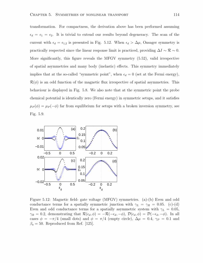
Chapter 5. Symmetries of nonlinear transport 114
transformation. For compactness, the derivation above has been performed assuming
ǫd = ǫ1 = ǫ2. It is trivial to extend our results beyond degeneracy. The scan of the
current with ǫd = ǫ1,2 is presented in Fig. 5.12. When ǫd > ∆µ, Onsager symmetry is
practically respected since the linear response limit is practiced, providing ∆I ∼ R ∼ 0.
More significantly, this figure reveals the MFGV symmetry (5.52), valid irrespective
of spatial asymmetries and many body (inelastic) effects. This symmetry immediately
implies that at the so-called “symmetric point”, when ǫd = 0 (set at the Fermi energy),
R(φ) is an odd function of the magnetic flux irrespective of spatial asymmetries. This
behaviour is displayed in Fig. 5.8. We also note that at the symmetric point the probe
chemical potential is identically zero (Fermi energy) in symmetric setups, and it satisfies
µP (φ) = µP (−φ) far from equilibrium for setups with a broken inversion symmetry, see
Fig. 5.9.
−0.5 0 0.5
−0.01
0
0.01
R
(a)
−0.2 0 0.2
0.05
0.1
0.15
0.2
D
(b)
−0.5 0 0.5−0.02
0
0.02
εd
R
(c)
−0.2 0 0.20.05
0.1
0.15
0.2
εd
D
(d)
Figure 5.12: Magnetic field- gate voltage (MFGV) symmetries. (a)-(b) Even and oddconductance terms for a spatially symmetric junction with γL = γR = 0.05. (c)-(d)Even and odd conductance terms for a spatially asymmetric system with γL = 0.05,γR = 0.2, demonstrating that R(ǫd, φ) = −R(−ǫd,−φ), D(ǫd, φ) = D(−ǫd,−φ). In allcases φ = −π/4 (small dots) and φ = π/4 (empty circle), ∆µ = 0.4, γP = 0.1 andβa = 50. Reproduced from Ref. [125].
Chapter 5. Symmetries of nonlinear transport 115
5.7 Relation of results to other treatments
Magnetic field symmetries of nonlinear transport were analyzed in several other papers
by including electron-electron interactions at different levels: mean field, Coulomb block-
ade, Kondo limit [110, 111, 112, 113]. Particularly, in Ref. [110] and more recent studies
[42] electron-electron interactions were taken into account by considering the nonlinear
response of the electronic potential landscape in the conductor to the applied voltage.
This is done by adopting scattering theory: The argument is that in a nonequilibrium
situation the charge density in the conductor piles up in response to the applied volt-
age. The scattering matrix then becomes bias dependent through its dependence on the
potential landscape in the conductor. Nonlinear conductance terms contain information
about charge response in the system, effects that are non-even in the magnetic field, and
this leads to deviations from Onsager’s reciprocity relation beyond linear response.
In our approach, we include interaction effects in the interior of the conductor within
an alternative approach, the probe. We recall that this tool emulates (electron-electron,
electron-phonon) interactions in the conductor as follows: First, we apply a bias and
set the temperatures at the two boundaries, µν , βν . We then include many body effects
at the conductor, e.g., inelastic effects, using a voltage probe, by demanding that the
charge current towards it vanishes. This constraint sets the probe parameters µP and
βP , describing charge distribution at the interior of the device. With these statistical
measures, chemical potentials and temperatures, we can calculate the charge current in
the Landauer picture. Our calculations provide us with the self-consistent probe chemical
potential, and this measure is generally neither even nor odd in the magnetic field, even
in linear response. Fig. 5.4 indeed shows that µP depends on the applied bias and
the magnetic flux, generally missing magnetic field symmetries. We can interpret the
probe potential as the local-internal potential in the conductor. We highlight that in our
approach we do not set it by hand. Rather, by setting boundary conditions for the L
and R terminals, and by imposing the probe constraint, we find the probe potential as a
Chapter 5. Symmetries of nonlinear transport 116
self-consistent solution.
We now argue that our analysis here, based on the probe technique, has a com-
parable status to the treatment of Ref. [110], and related studies, which are based
on the behaviour of the screening potential under bias. The screening potential is an
electrostatics-theory property; it responds to interactions between microscopic degrees of
freedom. Similarly, the probe potential is an effective statistical measure, describing the
internal potential, enclosing effects of microscopic scattering processes in the conductor.
Both the screening potential and the probe potential can be interpreted as the effects
of many body interactions and while these measures are not necessarily equivalent, they
both consistently incorporate effects beyond linear response: The screening potential is
written as an expansion in voltage, the probe potential is determined self consistently, at
arbitrarily large applied voltage.
In a recent study the wave-packet propagation in a top-down asymmetric Aharonov-
Bohm ring has been studied numerically by using the nonlinear Schrodinger equation
[130]. It has been shown that this Aharonov-Bohm ring can act as a diode even when
it is mirror symmetric and that it satisfies symmetry relations identical to those in our
work. Note that the inelastic voltage probe effectively introduces nonlinearity. In real
systems such nonlinearities may occur due to interactions: e-ph, e-e and interactions with
other impurities.
Fluctuation theorems and full counting statistics of nonlinear heat transport in a
three terminal system have been studied by means of a temperature probe in Ref. [131],
extracting leading order nonlinear thermal conductance term. The main argument in
this work is based on the assumption of separation of time scales; assuming that charge
fluctuations in the probe are much slower compared to the electron relaxation in the
probe, and the time-scales for transport in the conductor. Under this assumption, mag-
netic field symmetries of leading-order nonlinear thermal conductance coefficients were
obtained, and the presence of an antisymmetric (under the reversal of magnetic field)
Chapter 5. Symmetries of nonlinear transport 117
thermal conductance term has been demonstrated for a triple quantum dot Aharonov-
Bohm interferometer. This work supports our general proof of symmetry relations for
nonlinear heat transport, presented in Sec. 6.6.3.
We conclude this discussion by emphasizing that the derivation of symmetries beyond
linear response should be eventually done beyond phenomenological approaches and mean
field treatments, by adopting model Hamiltonians with genuine many body interactions
[113], and by using exact quantum techniques [132]. This will be the focus of the next
chapter.
5.8 Discussion
We have studied the role of elastic and inelastic scattering effects on magnetic field sym-
metries of nonlinear conductance terms using Buttiker’s probe technique. For spatially
symmetric junctions we proved the validity of the MF symmetries for charge transport,
D(φ) = D(−φ) and R(φ) = −R(−φ), though many body inelastic effects, introduced via
the probe, are asymmetric in the magnetic flux. We demonstrated the breakdown of these
MF symmetries when the junction has a left-right asymmetry, in the presence of inelastic
effects. Using a double-dot AB interferometer model we showed that it respects more
general MFGV symmetry relations, R(ǫd, φ) = −R(−ǫd,−φ) andD(ǫd, φ) = D(−ǫd,−φ).
We now recall that these sets of symmetries were derived only based on the symmetry
of the probe distribution function fP , upon reversal of the applied bias. Considering a
conductor coupled to a voltage probe and placed under both an applied temperature
bias and a voltage bias, we write the formal expansion IL = −IR =∑
n,mGn,m∆µn∆Tm
and identify R =∑
n+m=2k Gn,m∆µn∆Tm, to contain even conductance terms, and the
complementing term D =∑
n+m6=2k Gn,m∆µn∆Tm. Following the discussion of Secs.
5.4-5.5, we can immediately confirm the validity of the MF and the MFGV symmetries
implying that e.g. G1,1(φ) = −G1,1(−φ) for spatially symmetric setups.
Chapter 5. Symmetries of nonlinear transport 118
The rectification effect, of fundamental and practical interest, is realized by combining
many body interactions with a broken symmetry: broken spatial inversion symmetry or
a broken time reversal symmetry. Rectifiers of the first type have been extensively inves-
tigated theoretically and experimentally, including electronic rectifiers, thermal rectifiers
[44] and acoustic rectifiers [126]. In parallel, optical and spin rectifiers were designed
based on a broken time reversal symmetry, recently realized e.g. by engineering parity-
time meta-materials [127].
The model system investigated in Secs. 5.5-5.6, the double-dot AB interferometer,
offers a feasible setup for devising rectifiers based on broken time reversal symmetry: We
found that R 6= 0, when two conditions are simultaneously met: (i) the magnetic flux
obeys φ 6= 2πn, n is an integer, (ii) and the probe introduces inelastic effects. However,
when time reversal symmetry is maintained (when the flux obeys φ = 2nπ) our model
does not bring about the rectification effect, even if the spatial mirror symmetry is broken.
The technical reason is that in our minimal construction both dots are coupled to the L
and R metals directly, with an energy independent hybridization constant. In extended
models when the ring is coupled indirectly to the L and R metals, through a spacer state,
geometrical rectification may develop even in the absence of the threading magnetic flux.
It is of interest to verify the results of this work by adopting a microscopic model with
genuine many body interactions [133, 121, 123], by modeling a quantum point contact
[41, 43] or an equilibrated phonon bath, exchanging energy with the junction’s electronic
degrees of freedom. This could be done by extending numerical and analytic studies,
e.g., Refs. [101, 134, 25], to the nonlinear regime.
We conclude this work by highlighting potential applications of the probe technique
to far-from-equilibrium situations. In the linear response regime this self-consistent tool
has been proven extremely useful for investigating the ballistic to diffusive crossover in
electron [70, 85] and phonon transport [87, 88, 89]. While explicit analytic results are
missing beyond linear response, we have demonstrated here that one could still adopt
Chapter 5. Symmetries of nonlinear transport 119
this approach far from equilibrium and infer general transport symmetries, by analyzing
the properties of the probe. Our simulations confirm the stability of the self-consistent
numerical approach to far-from-equilibrium scenarios, and its utility for exploring trans-
port properties. As this technique is no longer limited to the linear response limit or to
weak (probe-conductor) coupling problems, it is now possible to explore its predictions
(e.g., the rectification behaviour) alongside quantum master equation approaches and
other treatments incorporating genuine elastic dephasing and inelastic effects. Future
studies will be devoted to the analysis of the thermoelectric effect under broken time
reversal symmetry [35, 36, 73, 25, 42, 135, 136] in the far-from-equilibrium regime, and
to the study of quantum transport, far from equilibrium, in networks with broken time
reversal symmetry [137].
Chapter 6
Microscopic approach: model III
6.1 Introduction
In the previous chapter, we obtained symmetry relations of nonlinear transport using phe-
nomenological probe models within the Landauer-Buttiker scattering formalism. We ar-
gued that the probes effectively emulate many body inetractions. Here we focus on model
III, a double-dot interferometer capacitively coupled to an equilibrium or a nonequilib-
rium fermionic environment. This setup is related to Buttiker’s voltage probe; energy
exchange processes are allowed, but particle leakage between the double-dot interferom-
eter and the fermionic environment is blocked. The main objectives of our work here are
(i) To study a genuine many body model and quantify magnetic field symmetries and
magnetoasymmetries of nonlinear transport. (ii) To test the qualitative predictions of
inelastic probe models studied in the previous chapter.
6.2 Model
The Hamiltonian of model III is written as
H = HAB +HF +Hint. (6.1)
120
Chapter 6. Microscopic approach: model III 121
where HAB is the double-dot system, Eqs (2.1)-(2.4), HF represents a fermionic environ-
ment which consists of a single level coupled to two metalic leads, refer to Eq. (2.9) and
Fig. 2.3, and Hint is the intreaction term between electrons in the double-dot and the
fermionic environment, assuming the form
Hint = Unpn1. (6.2)
Here np = c†pcp, n1 = a†1a1 are the number operators of a special level (p) in the fermionic
environemnt and dot ’1’ in the AB interferometer; U is the charging energy. The coupling
energy between the two dots (in the AB interferometer) and the leads can be absorbed
into the hybridization energy,
γL = 2π∑
l
ξβ,lδ(ω − ωl)ξ∗β′,l, γR = 2π
∑
r
ζβ,rδ(ω − ωr)ζ∗β′,r. (6.3)
Note that in our simulations, described below, we set the parameters γν and the electron
density of states in the metals, assumed to be a constant up to a sharp cutoff. We again
define the dot-reservoir hybridization energies for the fermionic environment system from
Eq. (2.9),
γs = 2π∑
s∈=±|gs|2δ(ω − ωs). (6.4)
Here s ∈ ± represents left (+) and right (-) leads in the fermionic environment.
The main observable of interest in this work is the charge current 〈I(t)〉 flowing
across the AB interferometer. We could separately simulate the currents at the L and
R terminals, but we choose to directly compute the expectation value of the averaged
current from a certain initial state up to the steady state limit. This measure satisfies
certain symmetries in the transient regime, as we show in Sec. 6.3.2. Simulations are
carried out using the numerically exact INFPI method. Our starting point is the formal
Chapter 6. Microscopic approach: model III 122
expression for the current,
〈I(t)〉 = Tr[ρI] = Tr[ρ(0)eiHtIe−iHt]. (6.5)
Here ρ is the total density matrix, and the trace is performed over all degrees of freedom
(AB and FE). As an initial condition, we select for convenience a factorized initial state
ρ(0) = σF (0)⊗ σAB(0) with σAB as the density matrix of the interferometer. We further
assume that σAB(t = 0) = σS(0) ⊗ σL ⊗ σR, with σS(0) as the reduced density matrix
of the double-dot within the AB interferometer. The FE is similarly prepared in a
factorized state with σF (0) = σp(0) ⊗ σ+ ⊗ σ−. The four reservoirs ξ = L,R,± are all
prepared in a grand canonical state with a given chemical potential and temperature,
ρξ = e−βξ(Hξ−µξNξ)/Tr[e−βξ(Hξ−µξNξ)]. In what follows we set all reservoirs at the same
temperatre β−1.
6.3 Numerical results
6.3.1 Charge current
The charge current in the interferometer, considering either an isolated case (U = 0) or
a dissipative case (U = 0.1) is presented in Fig. 6.1. We confirm that the former, a fully
coherent system, obeys phase rigidity, I(φ) = I(−φ), at all times. In contrast, when
the AB setup is coupled to a FE, the transient current and the steady state value do
not transparently expose any symmetry. This was indeed an early observation in several
relates studies: many body effects generate an internal potential that is not necessarily
phase symmetric, leading to the breakdown of linear response symmetries [110]. It can
be seen from Fig. 6.1 that the current through the AB interferometer increases when
the interferometer is capacitively coupled to a fermionic environment. This could be
reasoned by noting that the capacitive coupling modifies the interference pattern. Due
Chapter 6. Microscopic approach: model III 123
to the Coulomb energy shift of the bare dot energies (within a perturbative language)
the dots are not degenerate for nonzero U . Depending upon the position of dot levels
relative to the fermi energy of the metallic leads, opposite trends may be observed.
Before discussing the underlying magnetic field symmetries and magnetoasymmetries of
transport coefficients, we present an example of the convergence analysis in panel (c).
Here we display the current as a function of τc = δtNs in the transient regime, and after
steady state has been established. In both cases we confirm that results converge around
τc ∼ 1/∆µ. It should be noted that to approach the exact limit should control the time
step and the memory size, concurrently. This is because if we only increase the memory
length τc to infinity but maintain a fixed-finite timestep δt, the time discretization error
(Trotter) will accumulate as we add more terms into the truncated IF, deviating from
the exact limit. Thus, one should carefully monitor both the time-step and the memory
size for achieving reliable results, as was noted in the related QUAPI method [138].
6.3.2 Magnetic field dependence of transport coefficients
We now explore the underlying symemtries of the current using the data of Fig. 6.1,
by separating the current into its odd and even conductance terms. For the sake of
convienence we present the symmetry measures,
∆I(φ) ≡ 1
2[I(φ)− I(−φ)], (6.6)
R(φ) ≡ 1
2[I(φ) + I(φ)], (6.7)
D(φ) ≡ 1
2[I(φ)− I(φ)], (6.8)
where I(φ) is the current obtained upon interchanging the chemical potentials of the
left-right leads in the double-dot AB interferometer. From the power series expansion
of the current, Eq. (5.2), one can see that R(D) are even(odd) conductance terms. We
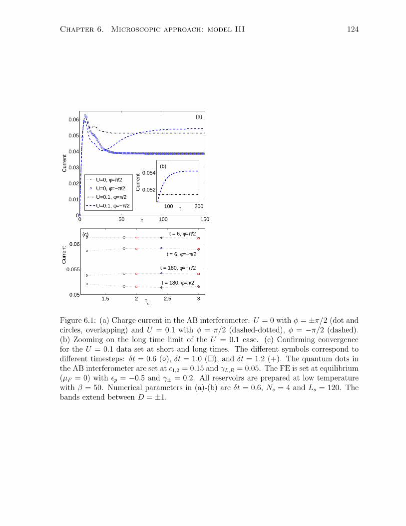
Chapter 6. Microscopic approach: model III 124
0 50 100 1500
0.01
0.02
0.03
0.04
0.05
0.06
t
Cur
rent
U=0, φ=π/2
U=0, φ=−π/2
U=0.1, φ=π/2
U=0.1, φ=−π/2 100 200
0.052
0.054
t
Cur
rent
(a)
(b)
1.5 2 2.5 30.05
0.055
0.06
t = 180, φ=π/2
t = 6, φ=π/2
τc
Cur
rent
t = 180, φ=−π/2
t = 6, φ=−π/2
(c)
Figure 6.1: (a) Charge current in the AB interferometer. U = 0 with φ = ±π/2 (dot andcircles, overlapping) and U = 0.1 with φ = π/2 (dashed-dotted), φ = −π/2 (dashed).(b) Zooming on the long time limit of the U = 0.1 case. (c) Confirming convergencefor the U = 0.1 data set at short and long times. The different symbols correspond todifferent timesteps: δt = 0.6 (◦), δt = 1.0 (�), and δt = 1.2 (+). The quantum dots inthe AB interferometer are set at ǫ1,2 = 0.15 and γL,R = 0.05. The FE is set at equilibrium(µF = 0) with ǫp = −0.5 and γ± = 0.2. All reservoirs are prepared at low temperaturewith β = 50. Numerical parameters in (a)-(b) are δt = 0.6, Ns = 4 and Ls = 120. Thebands extend between D = ±1.
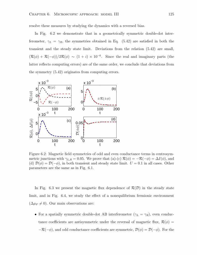
Chapter 6. Microscopic approach: model III 125
resolve these measures by studying the dynamics with a reversed bias.
In Fig. 6.2 we demonstrate that in a geometrically symmetric double-dot inter-
ferometer, γL = γR, the symmetries obtained in Eq. (5.42) are satisfied in both the
transient and the steady state limit. Deviations from the relation (5.42) are small,
(R(φ) + R(−φ))/2R(φ) ∼ (1 + i) × 10−6. Since the real and imaginary parts (the
latter reflects computing errors) are of the same order, we conclude that deviations from
the symmetry (5.42) originates from computing errors.
0 100 200
−5
0
5
x 10−3
t
R(±
φ)
R(φ)
R(−φ)
(a)
0 100 200
0
5
x 10−3
t
±R(±φ)
(b)
0 100 200
0
5
x 10−3
t
R(φ),∆I(φ) (c)
0 100 2000
0.05
t
D(±
φ)
(d)
Figure 6.2: Magnetic field symmetries of odd and even conductance terms in centrosym-metric junctions with γL,R = 0.05. We prove that (a)-(c) R(φ) = −R(−φ) = ∆I(φ), and(d) D(φ) = D(−φ), in both transient and steady state limit. U = 0.1 in all cases. Otherparameters are the same as in Fig. 6.1.
In Fig. 6.3 we present the magnetic flux dependence of R(D) in the steady state
limit, and in Fig. 6.4, we study the effect of a nonequilibrium fermionic environment
(∆µF 6= 0). Our main observations are:
• For a spatially symmetric double-dot AB interferometer (γL = γR), even conduc-
tance coefficients are antisymmetric under the reversal of magnetic flux, R(φ) =
−R(−φ), and odd conductance coefficients are symmetric, D(φ) = D(−φ). For the
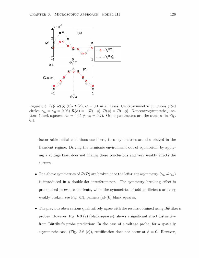
Chapter 6. Microscopic approach: model III 126
−1 0 10
0.05
0.1
φ/π
D
(b)
−1 0 1−2
0
2
4x 10
−3
R
(a)
φ/π
γL=γ
R
γL≠ γ
R
Figure 6.3: (a)- R(φ) (b)- D(φ), U = 0.1 in all cases. Centrosymmetric junctions (Redcircles, γL = γR = 0.05) R(φ) = −R(−φ), D(φ) = D(−φ). Noncentrosymmetric junc-tions (black squares, γL = 0.05 6= γR = 0.2). Other parameters are the same as in Fig.6.1.
factorizable initial conditions used here, these symmetries are also obeyed in the
transient regime. Driving the fermionic environment out of equilibrium by apply-
ing a voltage bias, does not change these conclusions and very weakly affects the
current.
• The above symmetries of R(D) are broken once the left-right asymmetry (γL 6= γR)
is introduced in a double-dot interferometer. The symmetry breaking effect is
pronounced in even coefficients, while the symmetries of odd coefficients are very
weakly broken, see Fig. 6.3, pannels (a)-(b) black squares.
• The previous observations qualitatively agree with the results obtained using Buttiker’s
probes. However, Fig. 6.3 (a) (black squares), shows a significant effect distinctive
from Buttiker’s probe prediction: In the case of a voltage probe, for a spatially
asymmetric case, (Fig. 5.6 (c)), rectification does not occur at φ = 0. However,
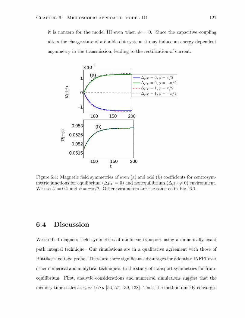
Chapter 6. Microscopic approach: model III 127
it is nonzero for the model III even when φ = 0. Since the capacitive coupling
alters the charge state of a double-dot system, it may induce an energy dependent
asymmetry in the transmission, leading to the rectification of current.
100 150 200
−1
0
1
x 10−3
R(±
φ)
100 150 200
0.0515
0.052
0.0525
0.053
t
D(±
φ)
∆µF = 0, φ = π/2
∆µF = 0, φ = −π/2
∆µF = 1, φ = π/2
∆µF = 1, φ = −π/2
(b)
(a)
Figure 6.4: Magnetic field symmetries of even (a) and odd (b) coefficients for centrosym-metric junctions for equilibrium (∆µF = 0) and nonequilibrium (∆µF 6= 0) environment.We use U = 0.1 and φ = ±π/2. Other parameters are the same as in Fig. 6.1.
6.4 Discussion
We studied magnetic field symmetries of nonlinear transport using a numerically exact
path integral technique. Our simulations are in a qualitative agreement with those of
Buttiker’s voltage probe. There are three significant advantages for adopting INFPI over
other numerical and analytical techniques, to the study of transport symmetries far-from-
equilibrium. First, analytic considerations and numerical simulations suggest that the
memory time scales as τc ∼ 1/∆µ [56, 57, 139, 138]. Thus, the method quickly converges
Chapter 6. Microscopic approach: model III 128
to the exact limit at large bias. Since we are specifically interested here in beyond-linear-
response situations, INFPI is perfectly suitable for the present situation. Second, our
objective here is in testing magnetic field symmetries in nonlinear transport, rather than
in studying particular features in the current-voltage curve. This task fits INFPI since it
is a deterministic time propagation scheme. Thus, even if simulation results deviate from
the exact limit to some extent, our conclusions are intact since I(+φ) and I(−φ) deviate
from the exact limit in an equivalent way. In contrast, methods that rely on stochastic
sampling of diagrams may accumulate distinct errors in the evaluation of I(±φ), thus
one may need to approach the exact limit for validating the symmetries (5.42). Finally,
INFPI is a flexible tool. We can readily test the nonlinear symmetry relations in the
class of models where the interacting part is given by the form Hint, Eq. (2.10). Future
work will focus on the study of magnetotransport in other correlated models.
Chapter 7
Conclusions and future directions
7.1 Summary
In this thesis we studied the transient dynamics and steady state properties of a double-
dot AB interferometer. In chapter 1, we introduced the physical realization of a parallel
double-dot setup, and outlined the general motivations behind this work. Three models
were introduced in chapter 2: (i) A double-dot interferometer with electron-electron in-
teractions, (ii) the case with Buttiker probes, and (iii) a double-dot setup capacitively
coupled to a fermionic environment. We also briefly presented the numerical and analyt-
ical techniques used in this work and discussed several open questions addressed in this
thesis.
The steady state properties and the transient dynamics of the noninteracting double-
dot interferometer were presented in chapter 3. Quantum Langevin equations were de-
rived, we solved these equations using the Green’s functions method, and resolved an
expression for the reduced density matrix in the steady state limit. We also followed the
transient dynamics using an exact fermionic trace formula. Using these tools we exposed
several non-trivial magnetic flux dependent effects: (i) flux dependent occupation dif-
ference at degeneracy, (ii) breakdown of phase localization away from the particle-hole
129
Chapter 7. Conclusions and future directions 130
symmetric point, and (iii) non-trivial transient features in the coherence dynamics. We
also studied the effect of temperature on the occupation difference.
We incorporated quasi-elastic dephasing effects in coherent dynamics using Buttiker’s
dephasing probe, obtained analytical expressions for dot occupations, and exposed sev-
eral magnetic flux dependent effects away from the symmetric point. For example we
demonstrated the development of new coherent oscillatory patterns when dot energies are
aligned with the Fermi energies of left/right leads. We also showed that at the symmetric
point the dots occupations are independent of the magnetic flux.
We incorporated an electron-electron repulsion term in chapter 4. Using INFPI, we
followed the transient dynamics of the reduced density matrix and charge current for
small-intermediate Coulomb interaction strengths. The dynamics in the infinite U limit
was studied using quantum master equations revealing fundamental deaviations from the
finite U case.
In chapter 5 we focused on magnetic field symmetries and magnetoasymmetries of
nonlinear transport coefficients. We showed that Onsager symmetries are obeyed be-
yond the linear response when elastic dephasing effects are in place, irrespetive of spatial
asymmetries. We also proved the absence of the diode effect in this case. We introduced
inelastic effects using Buttiker’s voltage probe, and showed that the Onsager symmetries
are obeyed in the linear regime, though the probe chemical potential need not be an even
function of the magnetic field. Using the voltage probe condition, exploiting the conser-
vation of transmission probabilities, we analytically showed that for a mirror symmetric
system, odd conductance terms (coefficients of odd powers in bias) are even in magnetic
flux while even terms (coefficients of even powers in bias) are odd.
We demonstrated these results using a model of double-dot interferometer. We also
proved that the same symmetries hold at the particle-hole symmetric point irresepctive
of spatial asymmetries. This analysis was also extended to describe a temperature and
a voltage-temperature probe. Away from the particle-hole symmetric point, introducing
Chapter 7. Conclusions and future directions 131
spatial asymmetries breaks the odd-even behaviour. We found that the symmetry break-
ing is more pronounced in even terms and the symmetries of odd terms are only weakly
broken. We established that the double-dot interferometer can act as a diode when two
conditions are met simultaneously: (i) many body effects are included, here in the form
of inelastic scattering, and (ii) time reversal symmetry is broken.
In chapter 6, we studied the dynamics and the steady state behaviour of magnetic
field symmetries and magnetoasymmetries in a double quantum dot interferometer ca-
pacitively coupled to a fermionic environment. Interestingly, we found that the results
obtained using inelastic probes do hold in this case. Our conclusions remain intact even
when the fermionic environment is driven out of equilibrium by applying a voltage bias.
7.2 Observations
We first focused on the dynamics and steady state behaviour of the reduced density
matrix and the charge current in the noninteracting case and exposed the nontrivial
interplay of magnetic flux, nonequilibrium effects and coherences:
• The occupations of the dots can be controlled by a magnetic flux away from the
symmetric point, and strong modulations are observed when the dots’ energies
are aligned with the fermi energy of the left/right leads. An abrupt jump in dot
occupations is observed when the magnetic flux takes values φ = 0, 2πn, where n
is an integer.
• The abrupt jump disappears at zero T only when the dot levels are positioned
far outside the bias window. Increasing the temperature, the jump reappears,
indicating the broadening of the resonance. Hence we can conclude that the abrupt
jump is a consequence of resonant tunneling.
• The energy degenerate and symmetrically coupled dots can have different occu-
pations in the presence of magnetic flux (φ 6= 2πn) when placed away from the
Chapter 7. Conclusions and future directions 132
symmetric point. The development of occupation difference is a generic finite-bias
effect, it disappears in the infinite bias limit when the transport is strictly unidi-
rectional. Increasing the temperature gradually reduces the occupation difference,
though it persists as long as the temperature is smaller than the system-bath hy-
bridization energy.
• The phase localization effect occurs when (i) the dots are placed at the symmetric
point, and (ii) in the infinite bias limit, when the dot levels are effectively at the
center of the bias window.
Buttiker probes offer an elegant phenomenological tool to introduce dephasing in
coherent transport. The dephasing probe condition allows one to compute the reduced
density matrix analytically. This simple system offers an interesting insights into how a
quasi-elastic dephasing affects the coherent transport. Considering the model of a double
dot interferometer, where one of the dots is coupled to a dephasing probe, we found that
away from the symmetric point the dot occupations can be controlled using a magnetic
flux, even in the presence of dephasing sources. we exposed the following nontrivial
effects:
• The abrupt jump observed in the occupation-flux behaviour disappears when de-
phasing effects are introduced.
• Away from the symmetric point, the occupations of the dots show flux dependent
modulations.
• When the dot levels are tuned at the edge of bias window, we find that the dot which
is coupled to a probe develops new types of coherent oscillations with magnetic flux.
The above phenomenon persists as long as the coupling to a dephasing probe is
smaller than the applied voltage bias.
Chapter 7. Conclusions and future directions 133
The dynamics of the interacting case is simulated using INFPI, and we have rigrously
established the utility of this method to study the long-time magnetic flux dependent
dynamics. At low temperatures the method does not converge if the bias is much smaller
than the strength of the Coulomb interaction. In the intermediate bias regime (∆µ > Γ),
and in weak-intermediate Coulomb interaction strengths (U/Γ ∼ 4) the dynamics of
coherences and charge current can be faithfully simulated. Our main findings are:
• The real part of the subsystem coherence ℜ(σ1,2) decays with magnetic flux depen-
dent rate Γ(1±cos(φ/2)) when φ 6= 2πn, while the imaginary part of the coherence
ℑ(σ1,2) settles to the steady state with a flux independent rate.
• The ℜ(σ1,2) is 4π periodic in magnetic flux and ℑ(σ1,2) is 2π periodic.
• Under a small-intermediate Coulomb interaction strengths (U/Γ ∼ 4), qualitative
characterstics of coherence dynamics are similar to the noninteracting case, while
in the U = ∞ limit the the transient dynamics significantly deaviates from the
noninteracting case, and the phase-localization effect breaks down.
• At φ = π destructive interference nullifies the charge current in the steady state
limit, irrespective of U and temperature of the leads.
Magnetic field symmetries of nonlinear transport were studied using the probe tech-
niques incorporating many body interactions. Our main findings are:
• Onsager symmetries are obeyed beyond linear response with quasi-elastic dephasing
irrespective of spatial asymmetries.
• The quasi-elastic dephasing probe does not allow for the diode effects, though the
time reversal symmetry and spatial symmetry are broken.
• Beyond linear response, inelastic interactions break the Onsager symmetries and
hence the phase rigidity.
Chapter 7. Conclusions and future directions 134
• Beyond the linear regime, the even conductance terms (coefficients of even bias
powers) are odd under the reversal of magnetic flux, while the odd terms (coef-
ficients of odd bias powers) are even if the setup is spatially and/or particle-hole
symmetric. These symmetries are broken away from the symmetric point, when
the spatial asymmetries are introduced.
• Our proof of symmetry relations for the mirror symmetric setups is general and we
did not assume any particular system Hamiltonian.
• In spatially asymmetric systems, the symmetry breaking is pronounced in even
conductance terms and the symmetries of odd terms are weakly broken.
• The double-dot interferometer acts as a diode when two conditions are simultane-
ously meet: (i) broken time reversal symmetry, and (ii) many body interactions
included in the form of inelastic scattering.
We studied magnetic field symmetries of the double-dot Aharonov-Bohm interferom-
eter capacitively coupled to a fermionic environment which may be out-of-equilibrium.
We argued that this setup is analogous to the voltage probe introducing inelastic ef-
fects. Numerical results for the transient and steady state magnetic field symmetries
were obtained using INFPI technique. We found that the observations derived from the
voltage probe do remain intact, irrespective of whether the fermionic environment is in
equilibrium or out-of-equilibrium.
7.3 Future work
Algorithmic improvements of INFPI: In this work we studied the transient dynamics of a
double-dot system using numerically exact path integral algorithm. We treated the many
body interaction term using the Hubbard Stratonovich (HS) transformation, the quartic
interaction is decomposed into quadratic terms by introducing an auxillary spin variable
Chapter 7. Conclusions and future directions 135
[154]. The main drawback of this procedure is that the time translation invariance of the
influence functional is lost, and it must be updated at every iteration. Such a scheme
is computationally expensive, limiting the practical applicability of the method. The
HS tranformation is unique if Uδt < π, where U is the strength of the electron-electron
interaction and δt is the time step chosen. If U is very large, then the time step should
be made very small, implying long simulation times.
INFPI technique without the HS tranformation was theoretically formulated using the
Hubbard basis in Ref. [56]. In this case the evaluation of the resulting trace is challenging
since matrix elements of nonquadratic operators enter the calculation. Future efforts will
be concentrated on resolving this issue so that one can study the dynamics in the U = ∞
case and in the Kondo regime.
Thermoelectricity: Future research will focus on nonlinear thermoelectric transport
in broken time reversal symmetric systems with many body interactions. Specifically, we
will study how various scattering mechanisms affect the maximum power efficiency. This
problem can be addressed using Buttiker’s probes. We will also attempt to modify exact
path integral methods to incorporate electron-phonon interactions. Such an extension will
be paramount for the study of thermoelectric transport in interacting systems, as much
work is done either using phenomenology or within the perturbative Green’s function
technique.
The effect of spatial asymmetries on coherence dynamics: In chapter 4 we focused on
the dynamics of coherences in degenerate and symmetric junctions. In a future project
we will focus on non-degenerate and spatially asymmetric systems, and study the effects
of many body interactions. Results from exact numerical calculations will be compared
to perturbative approaches.
Noise and correlations: It is of interest to compute current-current correlations and
higher order cumulants in interacting quantum dot networks using INFPI, comparing the
results with perturbative Keldysh techniques.

Chapter 7. Conclusions and future directions 136
Though this is a formal conclusion of the thesis, it is just the begining of a long and rich
effort to understand nonequilibrium phenomena which makes our life interesting. It is not
surprising that the understanding of nonequilibrium many body quantum phenomena is a
daunting task, but what is rather astonishing is our ability to create simplified theoretical
models to capture the essence of those effects.
I salute the imagination and ingenuity of Prof. Markus Buttiker who came up with
the interesting and valuable probe technique. It is sad that Prof. Buttiker is no longer
living with us, a huge intellectual loss for the field of quantum transport. Let him be in
a peace, and we should keep his legacy to advance this field, so that it will be always full
of excitement.

Bibliography
[1] Y. Aharonov, D. Bohm, Phys. Rev. 115, 481, (1959).
[2] G. Arfken and H. Weber, Mathematical methods for physicists.
[3] S. Washburn, R. Webb, Advances in Phys. 35 4 375 (1986).
[4] A. Yacoby, M. Heiblum, D. Mahalu, and H. Shtrikman, Phys. Rev. Lett. 74, 4047
(1995).
[5] A. W. Holleitner, C. E. Decker, H. Quin, K. Eberl, and R. H. Blick, Phys. Rev. Lett.
87, 256802 (2001).
[6] G. Hackenbroich, Phys. Rep. 343, 463 (2001), and references therein.
[7] R. Schuster, E. Buks, M. Heiblum, D. Mahalu, V. Umansky, and H. Shtrikman,
Nature 385, 417 (1997).
[8] J. Konig and Y. Gefen, Phys. Rev. Lett. 86, 3855 (2001); Phys. Rev. B 65, 045316
(2002).
[9] F. Li, X.-Q. Li, W.-M. Zhang, and S. A. Gurvitz, Euro. Phys. Lett. 88, 37001 (2009).
[10] Y. Tokura, H. Nakano, and T. Kubo, New J. Phys. 9, 113 (2007).
[11] Y.-S. Liu, H. Chen, and X.-F. Yang, J. Phys.: Condens. Matt. 19, 246201 (2007).
[12] D. Boese, W. Hofstetter, and H. Schoeller, Phys. Rev. B 66, 125315 (2002).
137
Bibliography 138
[13] D. Rai, O. Hod, and A. Nitzan, J. Phys. Chem. Lett. 2, 2118 (2011); Phys. Rev. B
85, 155440 (2012).
[14] M. Sigrist,T. Ihn, K. Ensslin, D. Loss, M. Reinwald, and W. Wegscheider, Phys.
Rev. Lett. 96, 036804 (2006).
[15] D. I. Golosov and Y. Gefen, New J. Phys. 9, 120 (2007).
[16] W. Hofstetter, J. Konig, and H. Schoeller, Phys. Rev. Lett. 87, 156803 (2001).
[17] Q.-F. Sun and H. Guo, Phys. Rev. B 66, 155308 (2002).
[18] J. Malecki and I. Affleck, Phys. Rev. B 82, 165426 (2010).
[19] O. Hod, R. Baer, and E. Rabani, Phys. Rev. Lett. 97, 266803 (2006).
[20] J. Verduijn, R. Agundez, M. Blaauboer, and S. Rogge, New J. Phys. 15, 033020
(2013).
[21] Y. Imry, Introduction to Mesoscopic Physics, 2nd ed. (Oxford University Press,
Oxford, 2002).
[22] F. Li, H.-J. Jiao, J.-Y. Luo, X.-Q. Li, and S. A. Gurvitz, Physica E 41, 1707 (2009).
[23] V. Kashcheyevs, A. Aharony, and O. Entin-Wohlman, Phys. Rev. B 73, 125338
(2006).
[24] A. Aharony and O. Entin-Wohlman, Phys. Rev. B 72, 073311 (2005).
[25] O. Entin-Wohlman and A. Aharony, Phys. Rev. B 85, 085401 (2012).
[26] D. Rai and M. Galperin, Phys. Rev. B 86, 045420 (2012).
[27] B. Kubala and J. Konig, Phys. Rev. B 65, 245301 (2002).
[28] D. Sztenkiel and R. Swirkowicz, J. Phys.: Condens. Matter 19 386224 (2007).
Bibliography 139
[29] Y.-S. Liu, H. Chen, and X.-F. Yang, J. Phys.: Condens. Matter 19 246201 (2007).
[30] D. Loss and E. Sukhorukov, Phys. Rev. Lett. 84, 1035, (2000).
[31] M. W.-Y. Tu, W.-M. Zhang, and J. Jin, Phys. Rev. B 83, 115318 (2011).
[32] M. W.-Y. Tu, W.-M. Zhang, J. Jin, O. Entin-Wohlman, and A. Aharony, Phys. Rev.
B 86, 11543 (2012).
[33] M. W.-Y. Tu, W.-M. Zhang, and F. Nori, Phys. Rev. B 86, 195403 (2012)
[34] S. Bedkihal and D. Segal, Phys. Rev. B 85, 155324 (2012).
[35] K. Saito, G. Benenti, G. Casati, and T. Prosen, Phys. Rev. B 84, 201306 (2011).
[36] V. Balachandran, G. Benenti, and G. Casati, Phys. Rev. B 87, 165419 (2013).
[37] L. Onsager, Phys. Rev. 37, 405 (1931); 38, 2265 (1931); H. B. G. Casimir, Rev.
Mod. Phys. 17, 343 (1945).
[38] J. Wei, M. Shimogawa, Z. Wang, I. Radu, R. Dormaier, and D. H. Cobden, Phys.
Rev. Lett. 95, 256601 (2005).
[39] R. Leturcq, D. Sanchez, G. Gotz, T. Ihn, K. Ensslin, D. C. Driscoll, and A. C.
Gossard, Phys. Rev. Lett. 96, 126801 (2006); R. Leturcq, R. Bianchetti, G. Gotz,
T. Ihn, K. Ensslin, D.C. Driscoll, and A. C. Gossard, Physica E 35, 327 (2006).
[40] L. Angers, E. Zakka-Bajjani, R. Deblock, S. Gueron, H. Bouchiat, A. Cavanna, U.
Gennser, and M. Polianski, Phys. Rev. B 75, 115309 (2007).
[41] D. Sanchez and K. Kang, Phys. Rev. Lett. 100, 036806 (2008).
[42] D. Sanchez and R. Lopez, Phys. Rev. Lett. 110, 026804 (2013); S. Hwang, D.
Sanchez, M. Lee, and R. Lopez, New Journal of Physics 15, 105012, (2013).
[43] V. I. Puller and Y. Meir, Phys. Rev. Lett. 104, 256801 (2010).
Bibliography 140
[44] M. Terraneo, M. Peyrard, and G. Casati, Phys. Rev. Lett. 88, 094302 (2002)
[45] D. Segal, and A. Nitzan, Phys. Rev. Lett. 94, 034301 (2005).
[46] C. Chang, D. Okawa, A. Majumdar, and A. Zettl, Science 314, 1121 (2006).
[47] L.D. Landau, Sov. Phys. JETP 3, 920 (1956); 5, 101 (1957); 8, 70 (1959).
[48] J. Kroha, P. Wolfle, Acta Physica Polonica 29, 12, (1998)
[49] Y. Chen, J. Stat. Phys. 47, 1, 1987
[50] P. Coleman, Introduction to Many Body Physics, (Cambridge University Press, 2012)
[51] D. Kollath, U. Schollwock and G. Vidal, J. Stat. Mech,: Theor. Exp. PO4005,
(2004).
[52] S.G. Jakobs, V. Menden, and H. Schoeller, Phys. Rev. Lett, 99, 150603, (2007).
[53] E. Gull, A. J. Millis, A. I. Lichtenstein, A. Rubtsov, M. Troyer, and P. Werner, Rev.
Mod. Phys. 83, 349 (2011).
[54] J. Han, R.J. Heary, Phys. Rev. Lett. 99, 236808 (2007).
[55] S. Weiss, J. Eckel, M. Thorwart, and R. Egger, Phys. Rev. B 77, 195316 (2008);
J. Eckel, F. Heidrich-Meisner, S. G. Jakobs, M. Thorwart, M. Pletyukhov, and R.
Egger, New J. Phys. 12, 043042 (2010).
[56] D. Segal, A. Millis, and D. Reichman, Phys. Rev. B 82, 205323 (2010).
[57] D. Segal, A. Millis, and D. Reichman, Chem. Phys. Phys. Chem 13, 14378 (2011).
[58] J. Schwinger, J. Math. Phys. 2, 407 (1961).
[59] L. Kadanoff and G. Baym, Quantum statistical mechanics (Benjamin/Cummings,
1962).
Bibliography 141
[60] L. Keldysh, Sov. Phys. JETP, 20, 1018 (1965).
[61] C. Caroli, R. Combescot, P.Nozieres, and D. Saint-James, J. Phys. C: Solid st. Phys,
4, 916 (1971).
[62] A. Dhar and D. Sen, Phys. Rev. B 73, 085119 (2006).
[63] R. Landauer, IBM J. Res. Dev. 1, 223 (1957).
[64] M. Buttiker, Phys. Rev. Lett. 57, 1761 (1986).
[65] S. Datta, Electric transport in Mesoscopic Systems (Cambridge: Cambridge Univer-
sity Press 1995).
[66] M. Buttiker, Phys. Rev. B 32, 1846 (1985); Phys. Rev. B 33, 3020 (1986).
[67] S. Andergassen, V. Meden, H. Schoeller, J. Splettstoesser, and M. R. Wegewijs,
Nanotechnology 21, 272001 (2010), and references therein.
[68] N. G. van Kampen, Stochastic processes in physics and chemistry, (North Holland,
1981).
[69] H.-P. Breuer and F. Petruccione, The Theory of Open Quantum Systems (Oxford
University Press, Oxford, UK, 2002).
[70] J. L. D’Amato and H. M. Pastawski, Phys. Rev. B 41, 7411 (1990).
[71] T. Ando, Surface Science 361, 270 (1996).
[72] P. A. Jacquet, J. Stat. Phys. 134, 709 (2009).
[73] K. Brandner, K. Saito, and U. Seifert, Phys. Rev. Lett. 110, 070603 (2013).
[74] J. P. Bergfield, S. M. Story, R. C. Stafford, and C. A. Stafford, ACS Nano 7, 4429
(2013).
Bibliography 142
[75] Y. Ming, Z. Wang, Z. Ding, H. Li, New J. Phys. 12, 103041 (2010).
[76] M. Bandyopadhyay and D. Segal, Phys. Rev. E 84, 011151 (2011).
[77] E. Pereira, H. C. F. Lemos, and R. R. Avila, Phys. Rev. E 84, 061135 (2011).
[78] P. Jacquet and C. Pillet, Phys. Rev. B 85, 125120 (2012).
[79] K. Saaskilahti, J. Oksanen, and J. Tulkki, Phys. Rev. E 88, 012128 (2013).
[80] P. Roulleau, F. Portier, P. Roche, A. Cavanna, G. Faini, U. Gennser, and D. Mailly,
Phys. Rev. Lett. 102, 236802 (2009).
[81] M. J. M. de Jong and C. W. J. Beenakker, Physica A 230, 219 (1996).
[82] S. A. van Langen and M. Buttiker, Phys. Rev. B 56, R1680 (1997).
[83] A. Hewson, The Kondo Problem to Heavy Fermions, (Cambridge University Press,
Cambridge, England, 1993).
[84] H.-L. Engquist and P. W. Anderson, Phys. Rev. B 24, 1151 (1981).
[85] D. Roy and A. Dhar, Phys. Rev. B 75, 195110 (2007).
[86] F. Bonetto, J. Lebowitz, and L. Rey-Bellet, Mathematical Physics 2000 (World
Scientific, Singapore, 2000), pp. 128150.
[87] F. Bonetto, J. L. Lebowitz, and J. Lukkarinen, J. Stat. Phys. 116, 783 (2004).
[88] A. Dhar and D. Roy, J. Stat. Phys. 125, 801 (2006).
[89] D. Roy, Phys. Rev. E 77, 062102 (2008).
[90] D. Segal, Phys. Rev. E 79, 012103 (2009).
[91] S. Pilgram, P. Samuelsson, H. Forster, and M. Buttiker, Phys. Rev. Lett. 97, 066801
(2006).
Bibliography 143
[92] H. Forster, P. Samuelsson, and M. Buttiker, New. J. Phys 9 117 (2007).
[93] M. Sindel, A. Silva, Y. Oreg and J. von Delft, Phys. Rev. B 72, 125316 (2005).
[94] H. Lee and S. Kim, Phys. Rev. Lett. 98, 186805 (2007).
[95] R. Bulla, T. Costi, and T. Pruschke, Rev. Mod. Phys. 80, 395 (2008).
[96] F. Anders and A. Schiller, Phys. Rev. Lett. 95, 196801 (2005); Phys. Rev. B 74,
245113 (2006); F. B. Anders, Phys. Rev. Lett. 101, 066804 (2008).
[97] G. Cohen and E. Rabani, Phys. Rev. B 84, 075150 (2011).
[98] D. Weinmann, Quantum transport through nanostructures Physikalisch-Technische
Bundesanstalt, PTB-Bericht PTB-PG-4, (1994).
[99] S. A. Gurvitz and Ya. S. Prager, Phys. Rev. B 53, 15932 (1996); S. A. Gurvitz, Phys.
Rev. B 57, 6602 (1998); S. A. Gurvitz, D. Mozyrsky, and G. P. Berman, Phys. Rev.
B 72, 205341 (2005).
[100] J. Kondo, Prog. Theo. Phys. 32, (1964).
[101] O. Hod, E. Rabani, and R. Baer, Acc. Chem. Res. 39, 109 (2006).
[102] K. Saito and Y. Utsumi, Phys. Rev. B 78, 115429 (2008).
[103] H. Linke, W. D. Sheng, A. Svensson, A. Lofgren, L. Christensson, H. Q. Xu, P.
Omling and P. E. Lindelof, Phys. Rev. B. 61, 15914 (2000).
[104] A. Lofgren, C. A. Marlow, I. Shorubalko, R. P. Taylor, P. Omling, L. Samuelson,
and H. Linke, Phys. Rev. Lett. 92, 046803 (2004).
[105] C. A. Marlow, R. P. Taylor, M. Fairbanks, I. Shorubalko, and H. Linke, Phys. Rev.
Lett. 96, 116801 (2006).
Bibliography 144
[106] D. M. Zumbhl and C. M. Marcus, M. P. Hanson and A. C. Gossard, Phys. Rev.
Lett. 96, 206802 (2006).
[107] M. Sigrist, T. Ihn, K. Ensslin, M. Reinwald, and W. Wegscheider, Phys. Rev. Lett.
98, 036805 (2007); T. Ihn, M. Sigrist, K. Ensslin, W. Wegscheider, and M. Reinwald,
New J. Phys. 9, 111 (2007).
[108] G. M. Gusev, Z. D. Kvon, E. B. Olshanetsky, and A. Y. Plotnikov, Europhys. Lett.
88, 47007 (2009).
[109] F. G. G. Hernandez, G. M. Gusev, Z. D. Kvon, and J. C. Portal, Phys. Rev. B 84,
075332 (2011).
[110] D. Sanchez and M. Buttiker, Phys. Rev. Lett. 93, 106802 (2004); M. Buttiker and
D. Sanchez, Int. J. Quantum Chem. 105, 906 (2005).
[111] B. Spivak and A. Zyuzin, Phys. Rev. Lett. 93, 226801 (2004).
[112] A. R. Hernandez and C. H. Lewenkopf, Phys. Rev. Lett. 103, 166801 (2009).
[113] J. S. Lim, D. Sanchez, and R. Lopez, Phys. Rev. B 81, 155323 (2010). Note that
in this work the authors used a different convention for the current expansion with
voltage, I = G0∆µ+G1∆µ2 + ....
[114] V. Puller, Y. Meir, M. Sigrist, K. Ensslin, and T. Ihn, Phys. Rev. B 80, 035416
(2009).
[115] S. Bedkihal, M. Bandyopadhyay, and D. Segal, Phys. Rev. B 87, 045418 (2013).
[116] Y. Meir and N. Wingreen, Phys. Rev. B 68, 2512 (1992).
[117] J. Franson, Non-equilibrium nano-physics, a many body approach, Lecture Notes in
Physics 809, Springer (2010).
Bibliography 145
[118] A. Batra, G. Kladnik, H. Vzquez, J.S. Meisner, L. Floreano, C. Nuckolls, D. Cvetko,
A. Morgante, L. Venkataraman, Nat. Comm. 3, 1086, (2012).
[119] I. Klich, in “Quantum Noise in Mesoscopic Systems”, edited by Yu. V. Nazarov
and Ya. M. Blanter (Kluwer, 2003).
[120] M. Pala and G. Iannaccone, Phys. Rev. B 69, 235304 (2004).
[121] A. Ueda and M. Eto, Phys. Rev. B 73, 235353 (2006); New J. of Phys. 9, 119
(2007); Physica E 40, 1602 (2008).
[122] Z. Zhu, A. Aharony, O. Entin-Wohlman, and P. C. E. Stamp, Phys. Rev. A 81,
062127 (2010).
[123] T. Kubo, Y. Tokura, and S. Tarucha, J. Phys. A: Math. Theor. 43, 354020 (2010).
[124] H. A. Nilsson, O. Karlstrm, M. Larsson, P. Caroff, J. N. Pedersen, L. Samuelson,
A. Wacker, L.-E. Wernersson, and H. Q. Xu , Phys. Rev. Lett. 104, 186804 (2010);
O. Karlstrom, J. N. Pedersen, P. Samuelsson, A. Wacker, Phys. Rev. B 83, 205412
(2011).
[125] S. Bedkihal, M. Bandyopadhyay, and D. Segal, Eur. Phys. J. B 86, 506 (2013).
[126] X.-F. Li, X. Ni, L. Feng, M.-H. Lu, C. He, and Y.-F. Chen, Phys. Rev. Lett. 106,
084301 (2011).
[127] L. Feng, Y.-L. Xu, W. S. Fegadolli, M.-H. Lu, J. E. B. Oliveira, V. R. Almeida,
Y.-F. Chen, and A. Scherer, Nature Materials 12, 108 (2013).
[128] S. Bedkihal, M. Bandyopadhyay, and D. Segal, Phys. Rev. B 88, 155407 (2013).
[129] V. Kashcheyevs. A. Schiller, A. Aharony, and O. Entin-Wohlman, Phys. Rev. B.
75, 115313 (2007).
[130] Y. Li, J. Zhou, F. Marchesoni, and B. Li, Scientific Reports, 4, 4566 (2014).
Bibliography 146
[131] Y. Utsumi, O. Entin-Wohlman, A. Aharony, T. Kubo, Y. Tokura, arXiv:1403.5582
[cond-mat.mes-hall], (2014).
[132] S. Bedkihal and D. Segal, unpublished.
[133] E. Deyo, B. Spivak, and A. Zyuzin, Phys. Rev. B 74, 104205 (2006).
[134] O. Hod, R. Baer, and E. Rabani, J. Phys. Condens. Matter 20, 383201 (2008).
[135] D. Sanchez and L. Serra, Phys. Rev. B 84, 201307(R) (2011).
[136] R. S. Whitney, Phys. Rev. B 87, 115404 (2013).
[137] Z. Zimboras, M. Faccin, Z. Kadar, J. Whitefield, B. Lanyon, and J. Biamonte,
Scientific Reports 3 2361, (2013).
[138] N. Makri, J. Math. Phys. 36, 2430 (1995).
[139] S. Weiss, R. Hutzen, D. Becker, J. Eckel, R. Egger, and M. Thorwart, Phys. Status
Solidi B 250, No. 11, 22982314 (2013).
[140] D. Gordon, M. Montemerlo, J. Love, G. Opiteck and J. Ellenbogen, Overview of
nanoelectronic devices, Proceedings of the IEEE, April 1997
[141] A. Schiller, E. Lebanon Phys. Rev. B. 65, 035308, (2001).
[142] E. Raikh, L. Glazman, Jetp Letters, 47, 8, 378 (1988).
[143] S. Pilgram, P. Samuelsson, H. Forster, and M. Buttiker, Phys. Rev. Lett. 97,
066801 (2006).
[144] H. Forster, P. Samuelsson, S. Pilgram, and M. Buttiker, Phys. Rev. B 75, 035340
(2007).
[145] M. Buttiker, Phys. Rev. B 46, 12485 (1992).
Bibliography 147
[146] R. Hartle, M. Butzin, O. Rubio-Pons, and M. Thoss, Phys. Rev. Lett. 107, 046802
(2011).
[147] S. Ballmann, R. Hartle, P. B. Coto, M. Elbing, M. Mayor, M. R. Bryce, M. Thoss,
and H. B. Weber, Phys. Rev. Lett. 109, 056801 (2012).
[148] J. S. Jin, M. W. Y. Tu, W. M. Zhang, and Y. J. Yan, New J. Phys. 12, 083013
(2010).
[149] M. Galperin, M. A. Ratner, and A. Nitzan, J. Phys.: Condens. Matter 19, 103201
(2007).
[150] P. Silvestrov and Y. Imry, Phys. Rev. Lett. 85, 2565 (2000); Phys. Rev. B 65,
035309 (2001).
[151] J. Konig and Y. Gefen, Phys. Rev. B 71, 201308(R) (2005).
[152] V. Meden and F. Marquardt, Phys. Rev. Lett. 96, 146801 (2006).
[153] C. Karrasch, T. Hecht, A. Weichselbaum, J. von Delft, Y. Oreg, and V. Meden,
New J. Phys. 9, 123 (2007).
[154] J. E. Hirsch, Phys. Rev. B 28, 4059 (1983).
[155] A. Polkovnikov, K. Sengupta, A. Silva, and M. Vengalattore Rev. Mod. Phys. 83,
863 (2011).
[156] I. L. Aleiner, N. S. Wingreen, and Y. Meir, Phys. Rev. Lett. 79, 3740 (1997).
[157] M. Buttiker, Phys. Rev. B 32, 1846 (1985); Phys. Rev. B 33, 3020 (1986), IBM J.
Res. Dev. 32, 63 (1988).
[158] T. Kubo, Y. Ichigo, and Y. Tokura, Phys. Rev. B 83, 235310 (2011).
[159] C. Bender S. Bttcher, Phys. Rev. Lett. 80, 5243 (1998).
Bibliography 148
[160] Z. Wang, Y. D. Chong, John D. Joannopoulos, and M. Soljacic PRL 100, 013905
(2008).
[161] W. H. Press, B. P. Flannery, S. A. Teukosky, and W. T. Vetterling, Numerical
Recipes in C: The Art of Scientific Computing, (Cambridge University Press 1992).
[162] Persistent currents exist in at thermal equilibrium due to the absence of time-
reversal symmetry. In our work here we consider only net charge transport. However,
since persistent currents are antisymmetric in the magnetic field, we could add them
to the defintion of R(φ), and our observations would be still valid.
[163] T. Kubo, Y. Tokura, and S. Tarucha, J. Phys. A: Math. Theor. 43, 354020 (2010).
[164] S. Hershfield, J. Davies, and J. Wilkins, Phys. Rev. B 46, 7046 (1992).