Quantum Simulation of 2D Quantum Chemistry in Optical Lattices

Javier Arguello-Luengo,1, ∗ Alejandro Gonzalez-Tudela,2, † Tao Shi,3, ‡ Peter Zoller,4, 5 and J. Ignacio Cirac6, 7, §

1ICFO-Institut de Ciencies Fotoniques, The Barcelona Institute ofScience and Technology, 08860 Castelldefels (Barcelona), Spain

2Instituto de Fısica Fundamental IFF-CSIC, Calle Serrano 113b, Madrid 28006, Spain3CAS Key Laboratory of Theoretical Physics, Institute of Theoretical Physics,

Chinese Academy of Sciences, P.O. Box 2735, Beijing 100190, China4Center for Quantum Physics, University of Innsbruck, A-6020 Innsbruck, Austria

5Institute for Quantum Optics and Quantum Information of the Austrian Academy of Sciences, Innsbruck, Austria.6Max-Planck-Institut fur Quantenoptik, Hans-Kopfermann-Straße 1, D-85748 Garching, Germany

7Munich Center for Quantum Science and Technology (MCQST), Munchen, Germany(Dated: February 24, 2020)

Benchmarking numerical methods in quantum chemistry is one of the key opportunities thatquantum simulators can offer. Here, we propose an analog simulator for discrete 2D quantumchemistry models based on cold atoms in optical lattices. We first analyze how to simulate simplemodels, like the discrete versions of H and H+

2 , using a single fermionic atom. We then show that asingle bosonic atom can mediate an effective Coulomb repulsion between two fermions, leading tothe analog of molecular Hydrogen in two dimensions. We extend this approach to larger systemsby introducing as many mediating atoms as fermions, and derive the effective repulsion law. In allcases, we analyze how the continuous limit is approached for increasing optical lattice sizes.

The field of theoretical quantum chemistry has expe-rienced an extraordinary progress due, in part, to manyadvances in computational methods [1]. For instance,Density Functional Theory [2, 3] has enabled a betterdescription and understanding of both static [4–7] anddynamic [8] properties of a large variety of molecules.The capability of such computational methods, whosemain challenge is to address electronic correlations, arehowever sometimes hard to assess experimentally. Oneapproach is to use another (classical) computational tech-nique that is exact in some restricted conditions, but candeal with large systems where exact calculations werenot possible. The most prominent example is DMRG [9]which, despite the fact that it operates in 1D lattice sys-tems, offers an ideal platform to benchmark DFT meth-ods [10–13]. In more general scenarios, the field of quan-tum computing [14–19] can play a key role to overcomenumerical limitations in the long-term, offering an ex-cellent setup to benchmark quantum chemistry compu-tational methods. Recently, we have proposed the al-ternative approach of analog quantum simulation [20],based on the experimentally mature field of ultra-coldatoms [21–23], where fermionic atoms play the role of theelectrons. While quantum computers and analog simu-lators would certainly help to push quantum chemistry,the exploration of their full potentiality requires the de-velopment of techniques that go beyond the state of theart.

In this Letter we propose and analyze a scheme foranalog quantum chemistry simulation that can be im-

∗ javier.arguello@icfo.eu† a.gonzalez.tudela@csic.es‡ tshi@itp.ac.cn§ ignacio.cirac@mpq.mpg.de

plemented with present technology. Our approach usesultracold atoms to address lattice models in two spatialdimensions (2D), where the electron-electron interactiontakes different forms. While not exactly reproducing allaspects of the real quantum chemistry scenario, this sim-ulator still retains the most relevant ingredients, enablingthe observation of the most representative phenomenain quantum chemistry. Furthermore, it offers a suitableplatform to benchmark computational methods in thatfield. In particular, it allows us to extend the bench-marking offered by DMRG beyond 1D [24].

For the sake of clarity, we will discuss several scenarios,with increasing experimental difficulty, for the simulationof quantum chemistry problems in 2D discrete latticesthat could later be compared to contemporary theoret-ical lattice methods, such as DFT or DMRG. We startwith simple one-electron systems, the analogous to theHydrogen atom, and the H+

2 molecule. Then, we showhow to simulate two electron problems, here exemplifiedby the H2 molecule. Finally, we show how the system canbe scaled-up to more electrons, although with a differentdependence of the repulsion with the distance.Model. In the following, we will consider a discrete

version of quantum chemistry models in 2D. First, westart by considering a 2D square optical lattice of sizeN×N . Nf fermionic atoms, playing the role of electrons,can localize within the local minima of this optical lattice,and hop with nearest-neighbor tunneling rate tF . TheHamiltonian describing their dynamics is then given by:

HK = −tF∑〈i,j〉

f†i fj , (1)

where f†i and fi, are the creation and annihilation op-erators for a fermionic atom in the i-th lattice site [28],each of them separated by a lattice spacing a, and where

arX

iv:2

002.

0937

3v1

[qu

ant-

ph]

21

Feb

2020

2

|ai|bi

|ai

trapped fermion

mediating boson

Ug

tbta

U

ta

a

c d

Optical lattice

d/a

Nuclear potential

b

Scheme I Scheme II

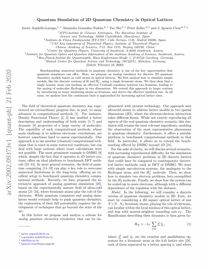
FIG. 1. Fermionic atoms (white) play the role of the molec-ular electrons. They hop in a 2D lattice (red), where thenuclear potential is imprinted (blue). For a single simulatedelectron, this pattern can lead to, e.g., atomic Hydrogen ((a),one nucleus) or H+

2 ((b), two nuclei). For more than onefermionic atom, two different schemes are proposed to medi-ate an effective repulsion between them. (c) A single atom(green) is used. It tunnels with constant ta through a lat-tice with the same spacing as the fermionic one. There is anon-site repulsion with strength U when the mediating atomoccupies the same site as the fermion. (d) We use as manymediating atoms as electrons need to be simulated (2 in thecase of the figure). The on-site repulsion with the fermionsnow appears in a different internal level b, whose tunneling isslower as compared to level a, using a state-dependent lattice.Both levels are coherently coupled with coupling constant g.

the sum is taken over all nearest-neighbor pairs of lat-tice sites. Fermionic atoms are subject to an externalpotential that induces the attraction to Nnuc nuclei thatwe consider placed in fixed positions {rn}n=1...Nnuc

[29](Born-Oppenheimer approximation [30]),

Hn({rn}) = −Nnuc∑n=1

∑j

ZnV (|j− rn|)f†i fj , (2)

where Zn is the atomic number of nucleus n, and V (r) isthe attractive nuclear potential [31]. In 2D lattices, thispotential can be obtained by combining the light shiftinduced by an external laser orthogonal to the lattice anda fully programmable intensity mask using, for example,a digital mirror device [32]. Depending on the modelto be simulated, we will also consider the HamiltonianHmed describing a set of bosonic atoms that mediatesfermion-fermion interactions according to some effectivepotential, Veff.

We consider now the simplest situation of simulat-ing atomic Hydrogen. By choosing a potential witha unique nucleus Z1 = 1 centered in the lattice site

r1 = (bN/2c, bN/2c + 1/2), the total Hamiltonian readsas,

H1 = HK +Hn(r1) . (3)

To begin with, we consider the attractive Coulomb po-tential on its standard form, V (r) = V0/r, for moder-ate finite lattice sizes, e.g. N = 40. In order to gainintuition, one can compare this discretized Hamiltonianto the continuum limit, where an analytical solution isalso known in 2D [33]. As a consequence of the reduceddimensionality, electrons get closer to the nuclei thanin the 3D case [34]. Each energy level corresponds to

E∗n = −Ry(n−1/2)2 , for n = 1, 2, . . . In that limit, one can

also identify,

a0/a = tF /V0 and Ry = V 20 /tF , (4)

that are the equivalent Bohr radius (a0), and Rydbergenergy (Ry), for the 2D discrete model [35]. The firstultimately determines the size of the orbitals and thushow the continuum limit is recovered. In particular, it isneeded that the orbitals fit in the lattice (to avoid finitesize effects), and that this Bohr radius occupies severallattice sites (to avoid discretization errors), leading to theinequalities,

N � tF /V0 � 1 . (5)

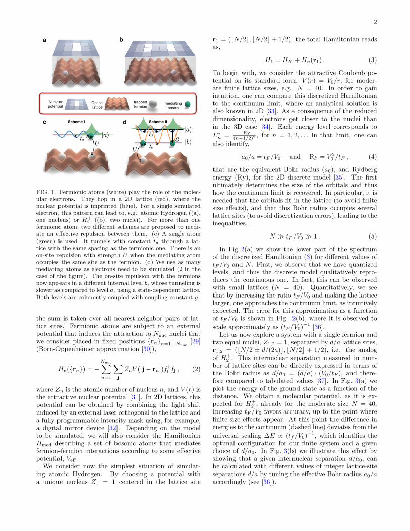
In Fig 2(a) we show the lower part of the spectrumof the discretized Hamiltonian (3) for different values oftF /V0 and N . First, we observe that we have quantizedlevels, and thus the discrete model qualitatively repro-duces the continuous one. In fact, this can be observedwith small lattices (N = 40). Quantitatively, we seethat by increasing the ratio tF /V0 and making the latticelarger, one approaches the continuum limit, as intuitivelyexpected. The error for this approximation as a functionof tF /V0 is shown in Fig. 2(b), where it is observed to

scale approximately as (tF /V0)−1

[36].Let us now explore a system with a single fermion and

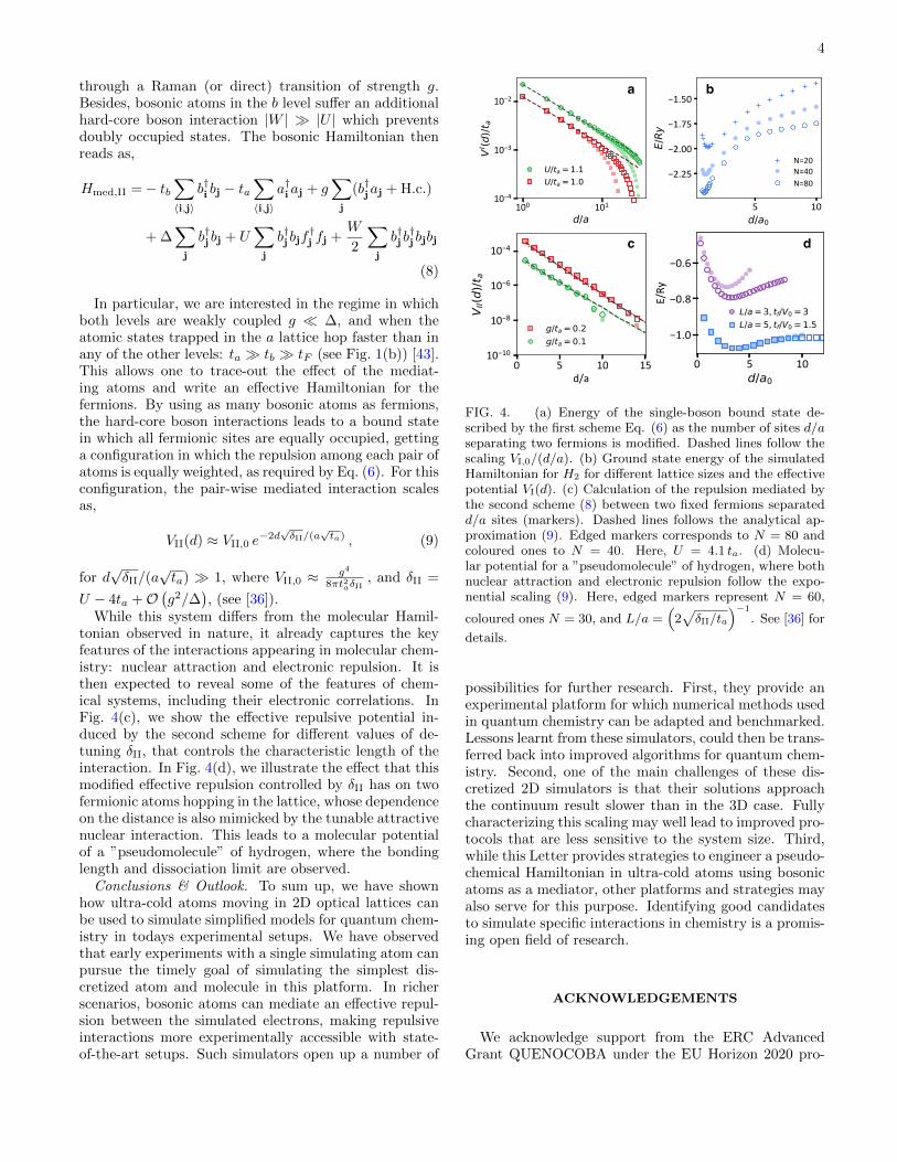
two equal nuclei, Z1,2 = 1, separated by d/a lattice sites,r1,2 = (bN/2 ± d/(2a)c, bN/2c + 1/2), i.e. the analogof H+

2 . This internuclear separation measured in num-ber of lattice sites can be directly expressed in terms ofthe Bohr radius as d/a0 = (d/a) · (V0/tF ), and there-fore compared to tabulated values [37]. In Fig. 3(a) weplot the energy of the ground state as a function of thedistance. We obtain a molecular potential, as it is ex-pected for H+

2 , already for the moderate size N = 40.Increasing tF /V0 favors accuracy, up to the point wherefinite-size effects appear. At this point the difference inenergies to the continuum (dashed line) deviates from the

universal scaling ∆E ∝ (tf/V0)−1

, which identifies theoptimal configuration for our finite system and a givenchoice of d/a0. In Fig. 3(b) we illustrate this effect byshowing that a given internuclear separation d/a0, canbe calculated with different values of integer lattice-siteseparations d/a by tuning the effective Bohr radius a0/aaccordingly (see [36]).

3

4Hydrogen2D_ED_atom1

n=1n=2n=3

Δ

a b

FIG. 2. (a) Lower part of the spectrum for the discretized2D atomic Hydrogen Hamiltonian in Eq. (3) for different val-ues of the effective Bohr radius tF /V0. As more lattice sitesare involved in the simulation (tF /V0 increases), the spec-trum approaches the value in the continuum (horizontal linesfor n = 1, 2, 3). This is valid up to a critical Bohr-radius inwhich finite-size effects become relevant and the solution de-viates from this behaviour. This critical value appears earlierfor smaller sizes (N = 40 for crossed markers) than for big-ger systems (N = 80, coloured marker, and N = 200, edgedmarker). (b) The energy difference ∆E between the ground-state of the discretized Hamiltonian in Eq. (3), and the onein the continuum decreases polynomially before finite-size ef-fects become relevant [36]. Larger system sizes can follow thisscaling up to more precise solutions. Dashed line follows thescaling (tF /V0)−1.

4HydrogenMas2D_ED_fig1

a b

FIG. 3. (a) Ground-state energy of the 2D hydrogen cation(H+

2 ) for different lattice sizes N and internuclear distanced/a0 (see Text for the optimal choice of the lattice separa-tion). The inset zooms into separation close to equilibrium.Dashed line (black crosses in the inset) follows an accurate so-lution for this 2D cation [37]. (b) Ground-state energy of H+

2

calculated for fixed d/a0 = 1 and increasing effective Bohrradius tF /V0. The solution decreases up to a critical size atwhich finite-size effects appear. This critical size is larger forbigger lattice sizes. In the inset, the difference in energies tothe tabulated value −1.41 Ry (black dashed line) reveals thescaling (tF /V0)−1 (red dashed line). Markers represent thesame sizes as in (a).

Two-fermions model. Let us now explore the situa-tion with two fermionic atoms emulating two electrons,where the interelectronic repulsion between them needsto be mediated. For this, we use an additional bosonicatom trapped in an optical lattice potential with thesame geometry as the fermions. First, we start with asimple scheme that only considers one of the bosonicinternal states, which allows them to tunnel at a rateta to nearest-neighboring sites. As they coexist in the

same lattice sites, elastic scattering processes betweenthe bosonic and fermionic atoms occupying the same po-sition induce an on-site repulsion U ,

Hmed,I = −ta∑〈i,j〉

a†i aj + U∑i

a†i aif†i fi , (6)

that translates into an effective repulsion between thefermions when the effect of the mediating atom is traced-out:

Hee =∑i,j

V (|i− j|)f†i fif†j fj , (7)

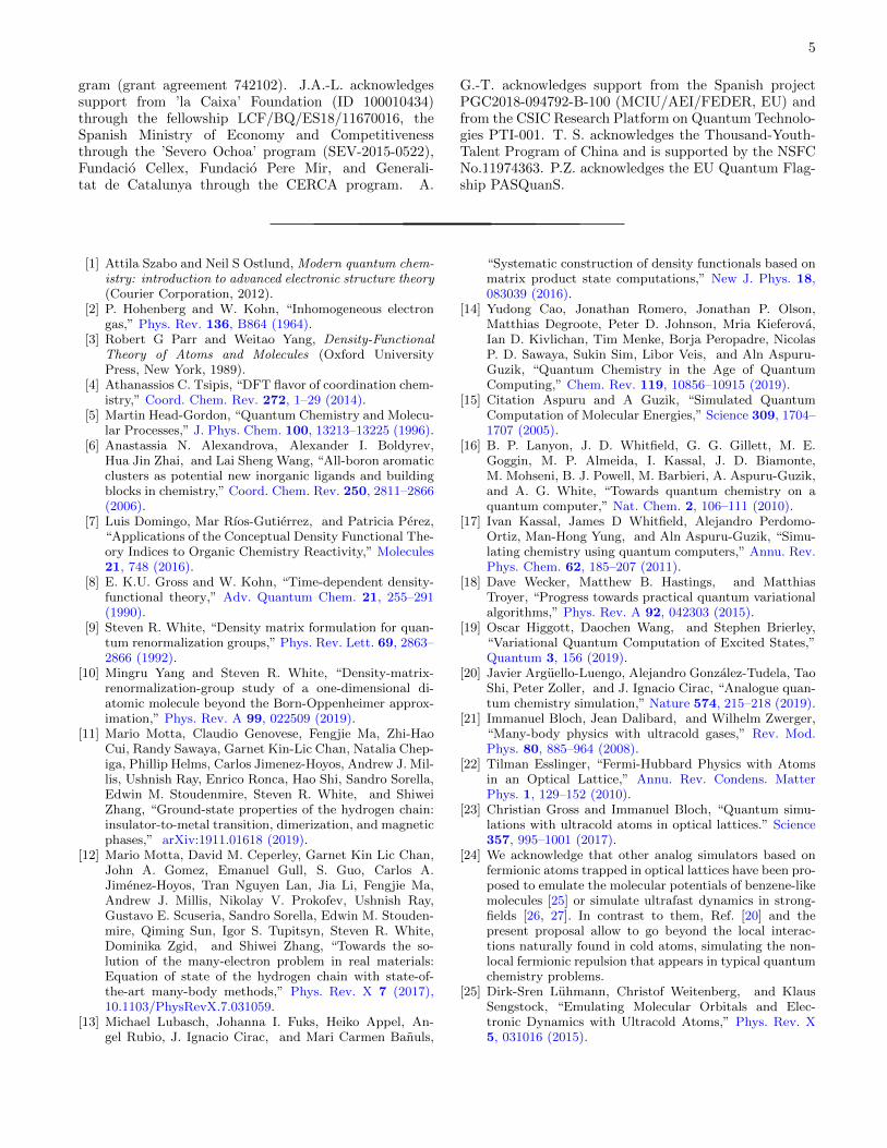
To obtain this expression, we assume to be in the regimein which the bosonic atom dynamics is faster than themovement of the fermions. In this first scheme, andfor separations d/a � 0.06 e2πta/U � N , this effec-tive repulsion corresponds to, VI(d) ≈ VI,0/(d/a) , where

VI,0 ≈ 6.4e−2πta/U ta (see [36]). This simple scheme thenmediates an effective repulsion between the two fermionicatoms that scales as 1/r, matching the dependence of thedistance of 3D molecular interactions, but now restrictedto 2D [38]. We illustrate the dependence of this potentialand its effect in the 2D H2 molecule in Figs. 4(a-b), re-spectively. There, one can observe molecular potentialsalso for relatively small lattices and assess the error. Thecontinuum limit is obtained in a similar regime than theH+

2 molecule case.Many-fermion models: By increasing the number of

fermionic atoms in the lattice while maintaining a singlemediating boson, one would see that not all interactionsamong pairs of fermions are equally weighted, precludingscalability. Intuitively, it is more favourable for the me-diating atom to localize among the pair of fermions thatare closer to each other, rather than in an equal superpo-sition, so that not all interaction are equally considered.In Ref. [20], this challenge was overcome by including acavity that symmetrizes these interactions. This cavityinteraction is not available in the present, much simplifiedexperimental setup, where interactions are mediated by ahopping atom, instead of a spin-excitation. Another op-tion to induce a pairwise effective repulsion between thesefermionic atoms would be Rydberg excitations, that en-able for long-range strong atomic interactions. In partic-ular, one can induce dipole-dipole repulsive interactionsthat depend on their separation as 1/d3 for distancessmaller than the Rydberg blockade radius [39–42].

Here instead, we present a second scheme that inducespair-wise interactions by including as many mediatingbosonic atoms as electrons need to be simulated. Thisproposal is scalable, at the price of modifying the scalingof the repulsive interaction (see Fig. 1(d)). For these Nfmediating atoms, we are going to consider two of its long-lived energy levels, that we call a and b, separated by anenergy shift ∆. Level b experiences an on-site repulsionU when occupying the same site as a fermion, while theatoms in level a live on a shallow lattice that allows themto move with tunneling rate ta. Both levels are coupled

4

through a Raman (or direct) transition of strength g.Besides, bosonic atoms in the b level suffer an additionalhard-core boson interaction |W | � |U | which preventsdoubly occupied states. The bosonic Hamiltonian thenreads as,

Hmed,II =− tb∑〈i,j〉

b†i bj − ta∑〈i,j〉

a†i aj + g∑j

(b†jaj + H.c.)

+ ∆∑j

b†j bj + U∑j

b†j bjf†j fj +

W

2

∑j

b†j b†j bjbj

(8)

In particular, we are interested in the regime in whichboth levels are weakly coupled g � ∆, and when theatomic states trapped in the a lattice hop faster than inany of the other levels: ta � tb � tF (see Fig. 1(b)) [43].This allows one to trace-out the effect of the mediat-ing atoms and write an effective Hamiltonian for thefermions. By using as many bosonic atoms as fermions,the hard-core boson interactions leads to a bound statein which all fermionic sites are equally occupied, gettinga configuration in which the repulsion among each pair ofatoms is equally weighted, as required by Eq. (6). For thisconfiguration, the pair-wise mediated interaction scalesas,

VII(d) ≈ VII,0 e−2d√δII/(a

√ta) , (9)

for d√δII/(a

√ta) � 1, where VII,0 ≈ g4

8πt2aδII, and δII =

U − 4ta +O(g2/∆

), (see [36]).

While this system differs from the molecular Hamil-tonian observed in nature, it already captures the keyfeatures of the interactions appearing in molecular chem-istry: nuclear attraction and electronic repulsion. It isthen expected to reveal some of the features of chem-ical systems, including their electronic correlations. InFig. 4(c), we show the effective repulsive potential in-duced by the second scheme for different values of de-tuning δII, that controls the characteristic length of theinteraction. In Fig. 4(d), we illustrate the effect that thismodified effective repulsion controlled by δII has on twofermionic atoms hopping in the lattice, whose dependenceon the distance is also mimicked by the tunable attractivenuclear interaction. This leads to a molecular potentialof a ”pseudomolecule” of hydrogen, where the bondinglength and dissociation limit are observed.

Conclusions & Outlook. To sum up, we have shownhow ultra-cold atoms moving in 2D optical lattices canbe used to simulate simplified models for quantum chem-istry in todays experimental setups. We have observedthat early experiments with a single simulating atom canpursue the timely goal of simulating the simplest dis-cretized atom and molecule in this platform. In richerscenarios, bosonic atoms can mediate an effective repul-sion between the simulated electrons, making repulsiveinteractions more experimentally accessible with state-of-the-art setups. Such simulators open up a number of

a b

c d

FIG. 4. (a) Energy of the single-boson bound state de-scribed by the first scheme Eq. (6) as the number of sites d/aseparating two fermions is modified. Dashed lines follow thescaling VI,0/(d/a). (b) Ground state energy of the simulatedHamiltonian for H2 for different lattice sizes and the effectivepotential VI(d). (c) Calculation of the repulsion mediated bythe second scheme (8) between two fixed fermions separatedd/a sites (markers). Dashed lines follows the analytical ap-proximation (9). Edged markers corresponds to N = 80 andcoloured ones to N = 40. Here, U = 4.1 ta. (d) Molecu-lar potential for a ”pseudomolecule” of hydrogen, where bothnuclear attraction and electronic repulsion follow the expo-nential scaling (9). Here, edged markers represent N = 60,

coloured ones N = 30, and L/a =(

2√δII/ta

)−1

. See [36] for

details.

possibilities for further research. First, they provide anexperimental platform for which numerical methods usedin quantum chemistry can be adapted and benchmarked.Lessons learnt from these simulators, could then be trans-ferred back into improved algorithms for quantum chem-istry. Second, one of the main challenges of these dis-cretized 2D simulators is that their solutions approachthe continuum result slower than in the 3D case. Fullycharacterizing this scaling may well lead to improved pro-tocols that are less sensitive to the system size. Third,while this Letter provides strategies to engineer a pseudo-chemical Hamiltonian in ultra-cold atoms using bosonicatoms as a mediator, other platforms and strategies mayalso serve for this purpose. Identifying good candidatesto simulate specific interactions in chemistry is a promis-ing open field of research.

ACKNOWLEDGEMENTS

We acknowledge support from the ERC AdvancedGrant QUENOCOBA under the EU Horizon 2020 pro-

5

gram (grant agreement 742102). J.A.-L. acknowledgessupport from ’la Caixa’ Foundation (ID 100010434)through the fellowship LCF/BQ/ES18/11670016, theSpanish Ministry of Economy and Competitivenessthrough the ’Severo Ochoa’ program (SEV-2015-0522),Fundacio Cellex, Fundacio Pere Mir, and Generali-tat de Catalunya through the CERCA program. A.

G.-T. acknowledges support from the Spanish projectPGC2018-094792-B-100 (MCIU/AEI/FEDER, EU) andfrom the CSIC Research Platform on Quantum Technolo-gies PTI-001. T. S. acknowledges the Thousand-Youth-Talent Program of China and is supported by the NSFCNo.11974363. P.Z. acknowledges the EU Quantum Flag-ship PASQuanS.

[1] Attila Szabo and Neil S Ostlund, Modern quantum chem-istry: introduction to advanced electronic structure theory(Courier Corporation, 2012).

[2] P. Hohenberg and W. Kohn, “Inhomogeneous electrongas,” Phys. Rev. 136, B864 (1964).

[3] Robert G Parr and Weitao Yang, Density-FunctionalTheory of Atoms and Molecules (Oxford UniversityPress, New York, 1989).

[4] Athanassios C. Tsipis, “DFT flavor of coordination chem-istry,” Coord. Chem. Rev. 272, 1–29 (2014).

[5] Martin Head-Gordon, “Quantum Chemistry and Molecu-lar Processes,” J. Phys. Chem. 100, 13213–13225 (1996).

[6] Anastassia N. Alexandrova, Alexander I. Boldyrev,Hua Jin Zhai, and Lai Sheng Wang, “All-boron aromaticclusters as potential new inorganic ligands and buildingblocks in chemistry,” Coord. Chem. Rev. 250, 2811–2866(2006).

[7] Luis Domingo, Mar Rıos-Gutierrez, and Patricia Perez,“Applications of the Conceptual Density Functional The-ory Indices to Organic Chemistry Reactivity,” Molecules21, 748 (2016).

[8] E. K.U. Gross and W. Kohn, “Time-dependent density-functional theory,” Adv. Quantum Chem. 21, 255–291(1990).

[9] Steven R. White, “Density matrix formulation for quan-tum renormalization groups,” Phys. Rev. Lett. 69, 2863–2866 (1992).

[10] Mingru Yang and Steven R. White, “Density-matrix-renormalization-group study of a one-dimensional di-atomic molecule beyond the Born-Oppenheimer approx-imation,” Phys. Rev. A 99, 022509 (2019).

[11] Mario Motta, Claudio Genovese, Fengjie Ma, Zhi-HaoCui, Randy Sawaya, Garnet Kin-Lic Chan, Natalia Chep-iga, Phillip Helms, Carlos Jimenez-Hoyos, Andrew J. Mil-lis, Ushnish Ray, Enrico Ronca, Hao Shi, Sandro Sorella,Edwin M. Stoudenmire, Steven R. White, and ShiweiZhang, “Ground-state properties of the hydrogen chain:insulator-to-metal transition, dimerization, and magneticphases,” arXiv:1911.01618 (2019).

[12] Mario Motta, David M. Ceperley, Garnet Kin Lic Chan,John A. Gomez, Emanuel Gull, S. Guo, Carlos A.Jimenez-Hoyos, Tran Nguyen Lan, Jia Li, Fengjie Ma,Andrew J. Millis, Nikolay V. Prokofev, Ushnish Ray,Gustavo E. Scuseria, Sandro Sorella, Edwin M. Stouden-mire, Qiming Sun, Igor S. Tupitsyn, Steven R. White,Dominika Zgid, and Shiwei Zhang, “Towards the so-lution of the many-electron problem in real materials:Equation of state of the hydrogen chain with state-of-the-art many-body methods,” Phys. Rev. X 7 (2017),10.1103/PhysRevX.7.031059.

[13] Michael Lubasch, Johanna I. Fuks, Heiko Appel, An-gel Rubio, J. Ignacio Cirac, and Mari Carmen Banuls,

“Systematic construction of density functionals based onmatrix product state computations,” New J. Phys. 18,083039 (2016).

[14] Yudong Cao, Jonathan Romero, Jonathan P. Olson,Matthias Degroote, Peter D. Johnson, Mria Kieferova,Ian D. Kivlichan, Tim Menke, Borja Peropadre, NicolasP. D. Sawaya, Sukin Sim, Libor Veis, and Aln Aspuru-Guzik, “Quantum Chemistry in the Age of QuantumComputing,” Chem. Rev. 119, 10856–10915 (2019).

[15] Citation Aspuru and A Guzik, “Simulated QuantumComputation of Molecular Energies,” Science 309, 1704–1707 (2005).

[16] B. P. Lanyon, J. D. Whitfield, G. G. Gillett, M. E.Goggin, M. P. Almeida, I. Kassal, J. D. Biamonte,M. Mohseni, B. J. Powell, M. Barbieri, A. Aspuru-Guzik,and A. G. White, “Towards quantum chemistry on aquantum computer,” Nat. Chem. 2, 106–111 (2010).

[17] Ivan Kassal, James D Whitfield, Alejandro Perdomo-Ortiz, Man-Hong Yung, and Aln Aspuru-Guzik, “Simu-lating chemistry using quantum computers,” Annu. Rev.Phys. Chem. 62, 185–207 (2011).

[18] Dave Wecker, Matthew B. Hastings, and MatthiasTroyer, “Progress towards practical quantum variationalalgorithms,” Phys. Rev. A 92, 042303 (2015).

[19] Oscar Higgott, Daochen Wang, and Stephen Brierley,“Variational Quantum Computation of Excited States,”Quantum 3, 156 (2019).

[20] Javier Arguello-Luengo, Alejandro Gonzalez-Tudela, TaoShi, Peter Zoller, and J. Ignacio Cirac, “Analogue quan-tum chemistry simulation,” Nature 574, 215–218 (2019).

[21] Immanuel Bloch, Jean Dalibard, and Wilhelm Zwerger,“Many-body physics with ultracold gases,” Rev. Mod.Phys. 80, 885–964 (2008).

[22] Tilman Esslinger, “Fermi-Hubbard Physics with Atomsin an Optical Lattice,” Annu. Rev. Condens. MatterPhys. 1, 129–152 (2010).

[23] Christian Gross and Immanuel Bloch, “Quantum simu-lations with ultracold atoms in optical lattices.” Science357, 995–1001 (2017).

[24] We acknowledge that other analog simulators based onfermionic atoms trapped in optical lattices have been pro-posed to emulate the molecular potentials of benzene-likemolecules [25] or simulate ultrafast dynamics in strong-fields [26, 27]. In contrast to them, Ref. [20] and thepresent proposal allow to go beyond the local interac-tions naturally found in cold atoms, simulating the non-local fermionic repulsion that appears in typical quantumchemistry problems.

[25] Dirk-Sren Luhmann, Christof Weitenberg, and KlausSengstock, “Emulating Molecular Orbitals and Elec-tronic Dynamics with Ultracold Atoms,” Phys. Rev. X5, 031016 (2015).

6

[26] Simon Sala, Johann Forster, and Alejandro Saenz,“Ultracold-atom quantum simulator for attosecond sci-ence,” Phys. Rev. A 95, 11403 (2017).

[27] Ruwan Senaratne, Shankari V. Rajagopal, Toshihiko Shi-masaki, Peter E. Dotti, Kurt M. Fujiwara, Kevin Singh,Zachary A. Geiger, and David M. Weld, “Quantumsimulation of ultrafast dynamics using trapped ultracoldatoms,” Nat. Commun. 9, 2065 (2018).

[28] Throughout the text, bold variables denote 2D vectors.[29] In order to prevent the divergence in the origin, positions

rn of the nuclei are shifted half a site from the latticenodes in the y direction.

[30] Considering that the electronic dynamics is much fasterthan the nuclear one, their equations can be decou-pled (Born-Oppenheimer approximation). The position{rn}i=n...Nn

of the Nn nuclei is considered fixed duringthe calculation of the electronic Hamiltonian Hcont, forthe Nf electrons in positions {ri}i=1...Nf

.

Hcont =−Nf∑i=1

~2

2me∇2

i −Nf∑i=1

1

2

Nn∑n=1

ZnV (|ri − rn|)

+

Nf∑i 6=j=1

V (|ri − rj |) ,

where me is the mass of the electron and Zn is the atomicnumber of nucleus n. The first term then describes thekinetic energy of the electrons, the second its nuclearattraction following the potential V (r) , and the thirdthe electronic repulsion.

[31] This externally induced potential could eventually mimicthe effect of inner-shell electrons as well.

[32] Jae-yoon Choi, Sebastian Hild, Johannes Zeiher, PeterSchauß, Antonio Rubio-Abadal, Tarik Yefsah, VedikaKhemani, David A Huse, Immanuel Bloch, and Chris-tian Gross, “Exploring the many-body localization tran-sition in two dimensions.” Science 352, 1547–52 (2016).

[33] B Zaslow and Melvin E Zandler, “Two-Dimensional Ana-log to the Hydrogen Atom Exact analytical solutions of atwo-dimensional hydrogen atom in a constant magneticfield,” Am. J. Phys. 35, 1118–1005 (1967).

[34] Jia-Lin Zhu and Jia-Jiong Xiong, “Hydrogen molecularions in two dimensions,” Phys. Rev. B 41, 12274–12277(1990).

[35] As compared to the three-dimensional case, Ry (2D) =4Ry (3D), and 2a0 (2D) = a0 (3D). Throughout the text,we will omit the (2D) labelling.

[36] See the Supplementary material accompanying this Let-ter. Section A discusses the scaling of the spectrum of thediscretized 2D Hamiltonian as the lattice size increases.Section B derives the effective interaction mediated by asingle boson with one long-lived state. Section C focuseson the effective interaction mediated by several mediat-ing atoms with two long-lived internal states. Section Dincludes further details about the numerical calculationsshown in Fig. 2-4.

[37] S. H. Patil, “Hydrogen molecular ion and molecule in twodimensions,” J. Chem. Phys. 118, 2197–2205 (2003).

[38] Note that this choice of nuclear potential differs from theone encountered in a flatland world, in which Coulomb’slaw leads to interactions that scale as ∝ log(r).

[39] M. D. Lukin, M. Fleischhauer, R. Cote, L. M. Duan,D. Jaksch, J. I. Cirac, and P. Zoller, “Dipole Block-

ade and Quantum Information Processing in MesoscopicAtomic Ensembles,” , 037901 (2000).

[40] Sylvain Ravets, Henning Labuhn, Daniel Barredo, LucasBeguin, Thierry Lahaye, and Antoine Browaeys, “Coher-ent dipole-dipole coupling between two single Rydbergatoms at an electrically-tuned Forster resonance,” Nat.Phys. 10, 914–917 (2014).

[41] M. Saffman, T. G. Walker, and K. Mølmer, “Quantuminformation with Rydberg atoms,” Rev. Mod. Phys. 82,2313–2363 (2010).

[42] However, the bare interaction is anisotropic in nature.[43] A. Heinz, A. J. Park, N. Santic, J. Trautmann, S. G.

Porsev, M. S. Safronova, I. Bloch, and S. Blatt,“State-dependent optical lattices for the strontium op-tical qubit,” arXiv:1912.10350 (2019).

[44] Shigetoshi Katsura and Sakari Inawashiro, “LatticeGreen’s Functions for the Rectangular and the SquareLattices at Arbitrary Points,” J. Math. Phys. 12, 1622–1630 (1971).

[45] M Abramowitz and I A Stegun, “Handbook of Math-ematical Functions with Formulas, Graphs and Mathe-matical Tables,” 9th printing, New York: Dover (1972).

[46] Stefan Schmid, Gregor Thalhammer, Klaus Winkler, Flo-rian Lang, and Johannes Hecker Denschlag, “Long dis-tance transport of ultracold atoms using a 1D opticallattice,” New J. Phys. 8, 159 (2006).

7

Appendix A: Discretization error in 2D

In Fig. 2 we observed that the discretized solutionsof the Hamiltonian approached the analytical result fol-lowing a scaling ∆E ∝ (tf/V0)

−1. This differs from the

three-dimensional case, in which accuracy improves as(tf/V0)

−2[20]. To analyze this effect, it is useful to have

some insights on how the discretization of the space af-fects the approach to the continuum solution. A back-of-the-envelope dimensional analysis can be presented forthe 2D case, where we consider the ground-state elec-tronic wave-function, ψ0(r) = a−1

0

√2/πe−r/a0 .

For the two main sources of discretization error, thecalculation of the energy terms is based on integrals thatare discretized as a Riemann sum. The difference be-tween this sum and the continuum limit is defined tofirst order by the second derivative of the integrand. Forthe Coulomb term, this reads as,

V0

∑j

∂2x

(|ψ(rj)|2/r

),

In the 2D case, this sum does not converge in the contin-uum limit, and the leading order error corresponds to thediverging term, that is dictated by our choice of the cut-off for the position closest to the nuclei. Normalizing bythe Rydberg energy, this error terms scales as (tf/V0)

−1

in 2D, and dominates the scaling of the 2D setup as theeffective Bohr radius increases, as numerically observed.

Appendix B: Single-level atom

1. Single boson localized around one fermion

As an introductory step to gain intuition, in this sec-tion we derive how a mediating boson affects the motionof a single fermion by localizing around it. This is thekey ingredient responsible for the effective repulsion ap-pearing when more than one fermion are present, thatwe derive in the next sections. In the limit tF /tB �1, one can make an approximation similar to Born-Oppenheimer. For a single fermion occupying the posi-tion j0, one can then expand the Hamiltonian H1B in the

basis |j0〉F |φj0〉B , where |j0〉F = f†j0 |0〉F and |φj0〉B is the

ground state of F 〈j| (H1B) |j〉F where, in the continuum

limit, H1B takes the form,∑

k ωka†kak + Ua†jajf

†j fj, be-

ing ω(k) = −2tb (cos kx + cos ky) the dispersion relationfor a free boson.

In the single fermion subspace, let us start choosingthe fermion to be positioned in j0 = 0 = (0, 0). The

eigenstate writes as β†λf†0 |0〉, where the bosonic operator

β†λ =∑

k φλ(k)a†k. The Schrodinger equation writes as,

ωk φ(k) + U φ(0) = EB φ(k), (B1)

where φ(j) = 1/N∑

k e−ikjφ(k).

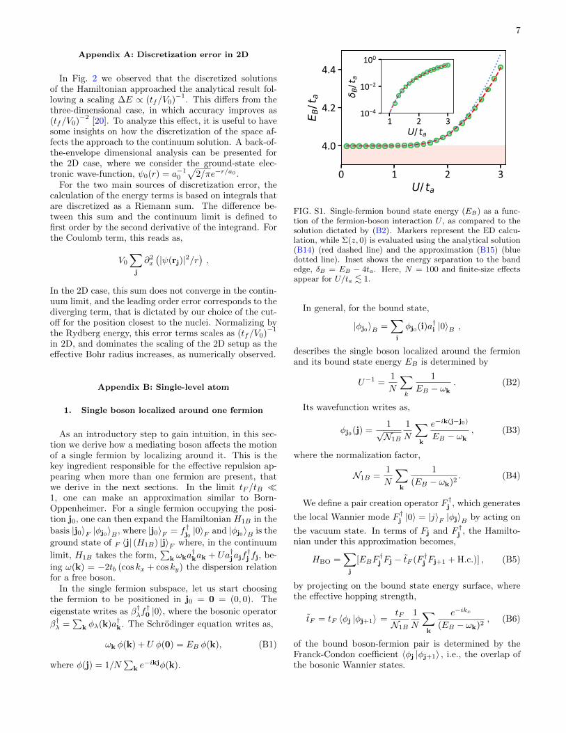
FIG. S1. Single-fermion bound state energy (EB) as a func-tion of the fermion-boson interaction U , as compared to thesolution dictated by (B2). Markers represent the ED calcu-lation, while Σ(z, 0) is evaluated using the analytical solution(B14) (red dashed line) and the approximation (B15) (bluedotted line). Inset shows the energy separation to the bandedge, δB = EB − 4ta. Here, N = 100 and finite-size effectsappear for U/ta <∼ 1.

In general, for the bound state,

|φj0〉B =∑i

φj0(i)a†i |0〉B ,

describes the single boson localized around the fermionand its bound state energy EB is determined by

U−1 =1

N

∑k

1

EB − ωk. (B2)

Its wavefunction writes as,

φj0(j) =1√N1B

1

N

∑k

e−ik(j−j0)

EB − ωk, (B3)

where the normalization factor,

N1B =1

N

∑k

1

(EB − ωk)2. (B4)

We define a pair creation operator F †j , which generates

the local Wannier mode F †j |0〉 = |j〉F |φj〉B by acting on

the vacuum state. In terms of Fj and F †j , the Hamilto-nian under this approximation becomes,

HBO =∑j

[EBF†j Fj − tF (F †j Fj+1 + H.c.)] , (B5)

by projecting on the bound state energy surface, wherethe effective hopping strength,

tF = tF 〈φj |φj+1〉 =tFN1B

1

N

∑k

e−ikx

(EB − ωk)2, (B6)

of the bound boson-fermion pair is determined by theFranck-Condon coefficient 〈φj |φj+1〉 , i.e., the overlap ofthe bosonic Wannier states.

8

2. Single boson localized around two fermions

By introducing a second fermion, the boson forms abound-state whose energy depends on this interfermionicseparation, inducing an effective repulsion between thesetwo fermions. Aided by the intuition gained in the pre-vious section, here we characterize the properties of thisbosonic bound-state.

In the single-boson subspace, the eigenstate writes

as β†λf†j1f†j2 |0〉, where the bosonic operator β†λ =∑

k φλ(k)a†k. The Schrodinger equation leads to

ωkφλ(k) + C1e−ikj1 + C2e

−ikj2 = Eλφλ(k), (B7)

with parameters,

C1 =U

N

∑k

eikj1φλ(k),

C2 =U

N

∑k

eikj2φλ(k). (B8)

The bound state solution

φ±(k) =C1e

−ikj1 + C2e−ikj2

E± − ωk, (B9)

of Eq. (B7) gives rise to the self-consistent equation

C1 =U

N

∑k

C1 + C2eikd

E± − ωk,

C2 =U

N

∑k

C1eikd + C2

E± − ωk, (B10)

which determines the relation C1 = ±C2. Focusing onthe bound state on the upper-band, that provides therepulsive interaction, and defining kx,y ≡ −π + kx,y, thebound state energy Eup corresponds to,

U−1 =1

N

∑k

1 + eikd

Eup − ωk

. (B11)

This equation encodes how the energy of the bound statedepends on the interfermionic separation. Note that d isa 2D-vector with integer components.

Equating (B2) and (B11), one gets,

1

N

∑k

1

EB − ωk=

1

N

∑k

1 + eikd

Eup − ωk

. (B12)

The solution to this equation admits a solution givenby a recurrence relation on d [44]. Using instead theexpansions derived in Sec. B 3 and B 4, one gets for d/a�1/√δB/ta),

δup = E+ − 4ta ≈2√δBd

e−γ , (B13)

where δB = EB − 4ta ≈ 25e−4πta/U ta , and γ ≈ 0.577 . . .is the Euler-Mascheroni constant.

This simple model then provides an effective repul-sion between the two fermions that scales as δup(d)/ta ∝V0,I/d with V0,I = 27/2e−γ−2πta/U ta.

From the wavefunction (B3) and the expansion in Sec.B 4 one sees that the characteristic length of the bound

states is LI/a ≈ (δB/ta)−1/2

. For the previous expan-sions in (B13) to be valid, one needs to satisfy the regimed/a� LI/a. To prevent finite size effects, it is also neces-sary, that LI/a� N . To illustrate this, in Fig. S1 we ob-serve that this expansion for δB/ta is valid for U/ta > 1,so that LI/a� N = 100. In Fig. S2 we also confirm thatfor this size, the scaling 1/d is maintained for d/a� 10,so that d/a� LI/a.

One can now see that this pairwise interaction doesnot maintain when more than two fermions are present.To reach this scalability, in Appendix C we will considera second internal level of the mediating atom.

3. Calculation of the first integral in (B11)

Defining the energy and length units ta ≡ 1, a ≡ 1 inthe coming sections, let us now calculate,

Σ(z, 0) =1

N2

∑k

1

z − ωk.

One can write an analytical solution [44],

Σ(z, 0) = 2K [4/z] /(πz) , (B14)

where K[m] =∫ π/2

0dθ(1−m2 sin2(θ)

)−1/2is the com-

plete elliptic integral of the first kind for |m| ≤ 1 [45].For values z = 4 + δ close to the band-gap (δ > 0 and|δ| � 1), one can define,

Σ(z, 0) ≈ (5 log 2− log δ)/(4π) +O(δ2). (B15)

4. Calculation of the second integral in (B11)

In order to extract the scaling of (B11) for frequenciesclose to the band-gap, it is useful to explore the continu-ous version of this sum. This will introduce a divergence,that was prevented by the natural cutoff of the lattice.

Now, we are interested in the calculation of,

Σ(z,d) =1

N2

∑k

eikd

z − ω(k), (B16)

for D = [0, 2π]⊗2

.In the limit kd � 1, we can expand the disper-

sion relation for frequencies close to the upper band-edge, [(kx, ky) = (π, π)]. Taking the translation kx,y ≡−π + kx,y, we expand ω(k) ≈ 4 − k2, and extend theintegration domain to infinite. Note that the numeratoreikd prevents the otherwise divergent integral, and thefrequency shift introduces a sign factor, eiπd, that does

9

not enter in the mediated potentials for the strategiespresented in this Letter. W.l.o.g., we align vector r inthe z-axis, and use spherical units,

Σ(z,d) = eiπdK0

[d√z − 4

]/(2π) , (B17)

where Kn[x] is the modified Bessel function of the secondkind [45] and d ≡ |d|. For small arguments (0 < x� 1),

K0[x] ≈ − log(x/2)− γ . (B18)

Appendix C: Mediating atoms with two long-livedstates

When more than two fermionic atoms are introduced,the effective repulsion mediated in the previous section bythe single-boson bound-state is not purely described bythe pair-wise separation between each pair of fermions.To gain this feature, let us introduce in this Section amodified scheme, where we consider two internal levelsof as many mediating atoms as fermions there are in thesystem. We will denote the two levels as b and a. Atomsin b level experience an on-site repulsion when occupy-ing the same site of a fermion, while atoms in state alive on a shallow lattice that allows them to hop withtunneling rate ta. Both levels are coupled through a Ra-man transition of strength g and are shifted by energy∆. In order to equally account for repulsion among eachpair of fermionic atoms, we include an on-site repulsionW among them when they occupy the same lattice site,obtaining the mediating Hamiltonian,

Hmed,II = ∆∑j

a†jaj − tb∑〈i,j〉

b†i bj − ta∑〈i,j〉

a†i aj

+ U∑j

b†j bjf†j fj + g

∑i

(b†jaj + H.c.) +W

2

∑j

b†j b†j bjbj .

(C1)

Intuitively, mediating atoms localize around thefermionic positions, and double occupations are pre-vented by the hard-core boson interaction W � U . Thisthen creates a bound-state in which each mediating atomlocalizes in a different fermionic position. As comparedto the previous scheme, hopping from one fermion to theothers now becomes a fourth-order process in the cou-pling g between the two atomic metastable states, as themovement of two mediating atoms is needed.

In particular, we are interested in the regime in whichboth levels are weakly coupled g/∆ � 1, and atomsin level a hop in a lattice much more shallow than therest: tf � tb � ta. As it occurred in the previouscase, this last inequality allows to trace-out the effectof the mediating atom, writing an effective Hamiltonian

for the fermions,∑

ij V (|i − j|)f†i fif†j fj. Let us now de-

rive this regime using perturbation theory for g/∆ � 1and Nf fermions occupying fixed positions j1 . . . jNf

. For

this, let us separate the bosonic Hamiltonian (C1), asHBN = H0 +HI , where

H0 =∆∑j

a†jaj − tb∑〈i,j〉

b†i bj − ta∑〈i,j〉

a†i aj

+ U∑j

b†j bjf†j fj +

W

2

∑j

b†j b†j bjbj ,

HI =g∑i

(b†jaj + H.c.) .

(C2)

In particular, we are interested in the energy correction

of the bound-state |ψB,II〉 =∏Nf

i=1 b†ji|0〉, that depends on

the interfermionic positions. For this, we need to expandthe perturbed Hamiltonian. One can see that only evenorders enter the calculation, and expanding to fourth or-der,

EB,II |ψB,II〉 =(H0 +HI

1

E −H0HI

+HI1

E −H0HI

1

E −H0HI

1

E −H0HI

)|ψB,II〉 ,

(C3)

one gets the equation,

EB,II = NfU +Nfg2

N2

∑k

1

EB,II/Nf −∆− ωk

+2g4

N4

Nf∑i6=j=1

∑k,q

1 + ei(k−q)(ri−rj)

(EB,II/Nf −∆− ωk)2

(EB,II/Nf −∆− ωq).

(C4)

This latter term originates from the pairwise repulsionintroduced by the fourth-order correction of two mediat-ing atoms swapping the fermionic position they localizearound. This then leads to an effective pairwise poten-

tial,∑Nf

i6=j=1 VII(|ri − rj)|)f†i fif†j fj, where

VII(d) ≈2g4

N4

(∑k

eikd

(EB,II/Nf −∆− ωk)2

)

×(∑

q

e−iqd

EB,II/Nf −∆− ωq

).

(C5)

These two independent sums can be calculated asin Sec. B 4. Note that the alternating sign derivedin Sec. B 4 cancels after the double product eikde−iqd.Using that ∂xK0[x] = −K1[x], one obtains, VII(d) ≈

2g4

(2π)2K0

[d√δII]

d2√δIIK1

[d√δII], which, to lowest order

in the regime d√δII > 1, scales as,

VII(d) ≈ g4

8πδIIe−2d

√δII . (C6)

This then leads to a pairwise repulsion between thefermionic atoms that decays exponentially with their sep-

aration, following a decay length LII ≡(2√δII)−1/2

. In

10

a b

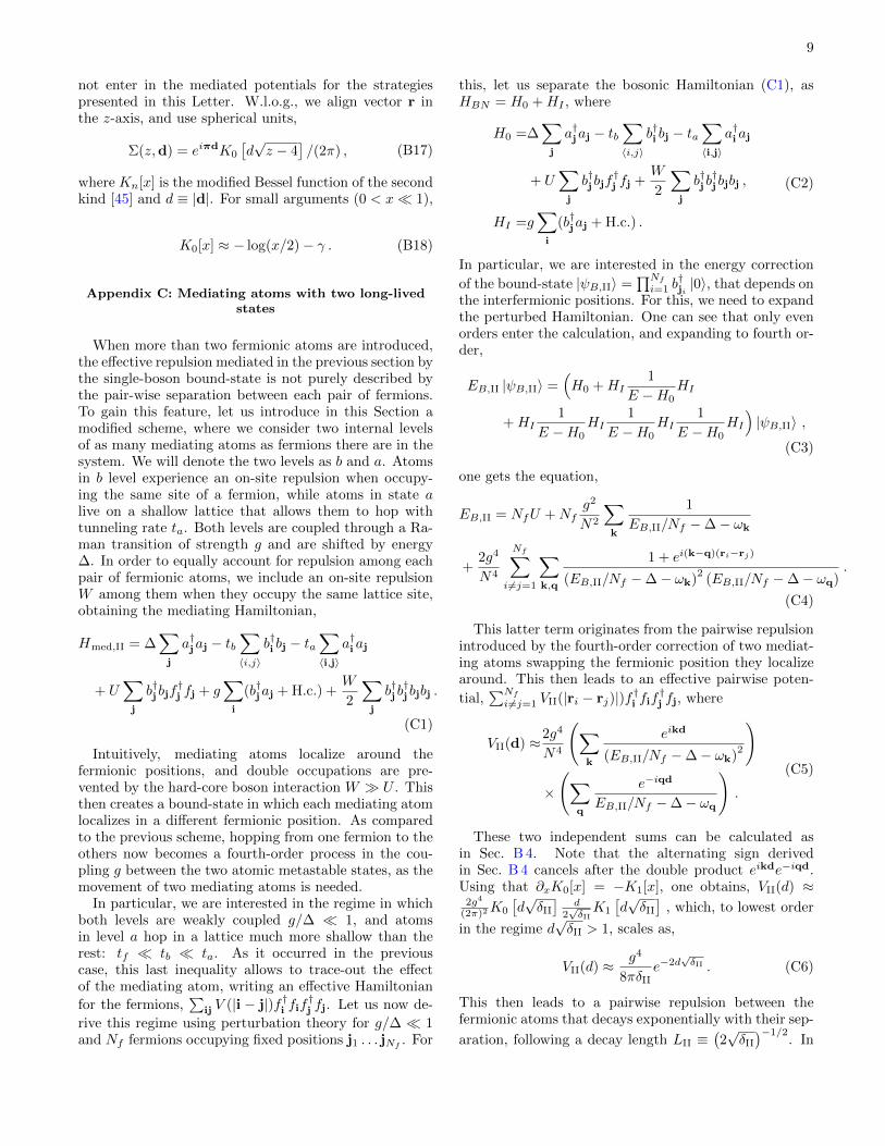
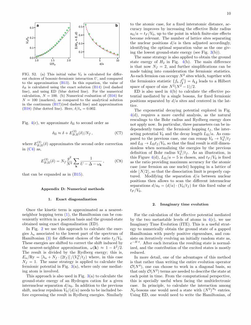
FIG. S2. (a) This initial value V0 is calculated for differ-ent choices of bosonic-fermionic interaction U , and comparedto the approximation (B13). In this equation, the value ofδB is calculated using the exact solution (B14) (red dashedline), and using ED (blue dotted line). For the numericalcalculation, N = 100. (b) Numerical evaluation of (B16) forN = 100 (markers), as compared to the analytical solutionin the continuum (B17)(red dashed line) and approximation(B18) (blue dotted line). Here, δ/ta = 0.002.

Fig. 4(c), we approximate δII to second order as

δII ≈ δ + E(2)B,II(δ)/Nf , (C7)

where E(2)B,II(δ) approximates the second order correction

in (C4) as,

E(2)B,II(δ) = Nf

g2

N2

∑k

1

U −∆− ωk, (C8)

that can be expanded as in (B15).

Appendix D: Numerical methods

1. Exact diagonalization

Once the kinetic term is approximated as a nearest-neighbor hopping term (1), the Hamiltonian can be con-veniently written in a position basis and the ground-stateobtained using exact diagonalization (ED).

In Fig. 2 we use this approach to calculate the ener-gies λn associated to the lowest part of the spectrum ofHamiltonian (3) for different choices of the ratio tf/V0.These energies are shifted to correct the shift induced bythe nearest-neighbor approximation, ω(k) ≈ 1 − k2/2.The result is divided by the Rydberg energy; this is,En/Ry = [λn +Nf · (2tf )] /(V 2

0 /tf ) where, in this caseNf = 1. The same strategy is applied to calculate thefermionic potential in Fig. 3(a), where only one mediat-ing atom is involved.

This approach is also used in Fig. 3(a) to calculate theground-state energy of an Hydrogen cation for a giveninternuclear separation d/a0. In addition to the previousshift, nuclear repulsion V0/(d/a) needs to be included be-fore expressing the result in Rydberg energies. Similarly

to the atomic case, for a fixed interatomic distance, ac-curacy improves by increasing the effective Bohr radiusa0/a = tF /V0, up to the point in which finite-size effectsbecome relevant. The number of lattice sites separatingthe nuclear positions d/a is then adjusted accordingly,identifying the optimal separation value as the one giv-ing the lowest ground-state energy (see Fig. 3(b)).

The same strategy is also applied to obtain the groundstate energy of H2 in Fig. 4(b). The main differenceis that now Nf = 2, and further simplifications can bemade taking into consideration the fermionic statistics.As each fermion can occupyN2 sites which, together with

the fermionics statistic {fi, f†j } = δi,j leads to a Hilbert

space of space of size N2(N2 − 1)/2.ED is also used in 4(b) to calculate the effective po-

tential mediated by a single bosons, for fixed fermionicpositions separated by d/a sites and centered in the lat-tice.

The exponential decaying potential explored in Fig.4(d), requires a more careful analysis, as the naturalrescalings to the Bohr radius and Rydberg energy doesnot apply now. In particular, three parameters can be in-dependently tuned: the fermionic hopping tf , the inter-acting potential V0 and the decay length LII/a. As com-pared to the previous case, one can remap V0 → V 2

0 /tfand LII → LIItf/V0, so that the final result is still dimen-sionless when normalizing the energies by the previousdefinition of Bohr radius V 2

0 /tf . As an illustration, inthis Figure 4(d), LII/a = 5 is chosen, and tF /V0 is fixedas the ratio providing maximum accuracy for the atomiccase (one fermion an one nuclei) hopping in a lattice ofside bN/2c, so that the dissociation limit is properly cap-tured. Modifying the separation d/a between nuclearpositions then allows to scan the different internuclearseparations d/a0 = (d/a) · (V0/tf ) for this fixed value oftF /V0.

2. Imaginary time evolution

For the calculation of the effective potential mediatedby the two metastable levels of atoms in 4(c), we useImaginary Time Evolution (ITE). This is a useful strat-egy to numerically obtain the ground state of a gappedHamiltonian with purely positive eigenvalues, and con-sists on iteratively evolving an initially random state as,e−H·t. After each iteration the resulting state is normal-ized, and the contribution of the excited states is mostlyreduced.

In more detail, one of the advantages of this methodis that rather than writing the entire evolution operatorO(N4), one can choose to work in a diagonal basis, sothat onlyO(N2) terms are needed to describe the state ateach point in time. From the computational perspective,this is specially useful when facing the multielectroniccase. In principle, to calculate the interaction amongNb-bosons one would need a state with (N2)Nb entries.Using ED, one would need to write the Hamiltonian, of

11

size (N2)Nb × (N2)Nb . In contrast, evolving the state inimaginary time evolution only needs to store the diagonalterms [with size (N2)Nb ], once the state is expressed in abasis that commutes with the terms of the Hamiltonian.For our particular case, this corresponds to the positionrepresentation for the on-site interactions, and momen-tum representation for the kinetic term. The Hamilto-nian Hnuc is already diagonal in position basis, and onecan define a momentum basis,

f†k(b†k) =1

N

∑j

e−ikjf†j (b†j ) , (D1)

where HK reads as HK =∑

k ωk,ff†kfk, being ωk,f =

−2tF (cos(kx) + cos(ky)) the dispersion relation. This in-duces a periodic boundary condition in the lattice, whichdoes not affect the calculation as long as finite-size ef-fects are prevented. To confirm that is the case, for eachchoice of parameters we check that the same result isobtained for the single-boson case using ED, evidencingthat boundary conditions are not affecting the result.

To calculate the ITE of Hamiltonian (8), a constantenergy shift is added to H during the calculation to makeall the spectrum positive, which is later subtracted at theend of the calculation. To evaluate the operation, ψ(t) =e−Htψ(0) we use a Suzuki-Trotter [46] expansion of thefirst kind, dividing the evolution in n steps as e−Ht ≈∏n−1k=1 e

−H∆t + O (∆t), and tk = k · ∆t/t. For each ofthese steps, we calculate

e−H∆tψ(tk) ≈IFFT[e−HK∆t FFT

(e−HR∆te−Hg∆tψ(tk−1

)]+O

(∆t2

),

(D2)

where (I)FFT indicates the (Inverse) Fast Fourier Trans-formation, and normalize the resulting state. Here, HR

denote the terms that are diagonal in the position basis,and HK the ones in momentum basis. Hg denotes thecoupling term, whose exponential can be directly calcu-

lated noting that, e−g(a†j bj+H.c.)∆t = cosh(g∆t)(a†jaj +

b†j bj)− sinh(g∆t)(a†j bj + H.c.). We iterate this procedure

until the overlap between ψ(tk−1) and ψ(tk) is smallerthan 10−5. We initialize the algorithm with a randomstate for the smallest value of tF /V0, and use this con-verged solution as the initial state for the next configu-ration of tF /V0.

In our second scheme, Nf atoms with two long-livedstates are used to mediate the interaction among Nffermions. For a given fermionic configuration, we desireto numerically calculate the bound state, and compareit to the analytical expansion previously introduced inEq. (C5). For this calculation, we use the ITE method(Sec. D 2), where now, each of the Nf mediating atomscan occupy any of the 2 levels at any of the N2 latticesites, which a priori accounts for states of size (2N2)Nf .To reduce this space, we assume that |g/(U −∆)| � 1,so that level b is only populated in the sites where they

0 100

5

10

15

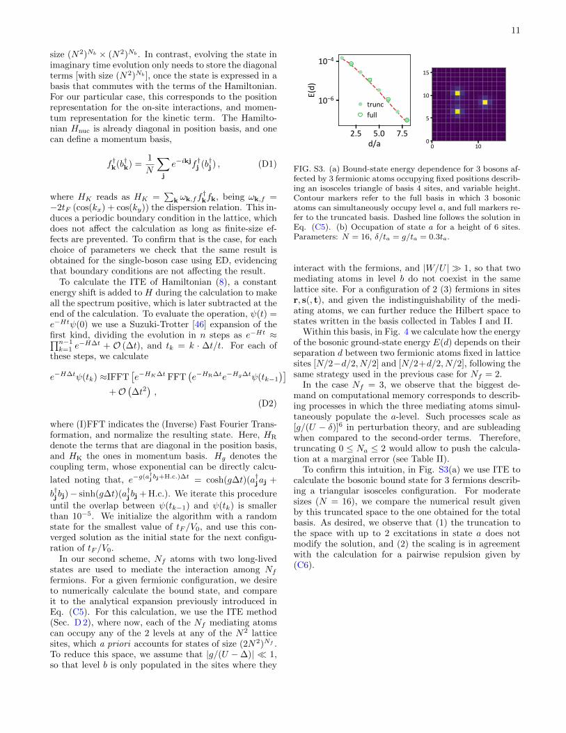
FIG. S3. (a) Bound-state energy dependence for 3 bosons af-fected by 3 fermionic atoms occupying fixed positions describ-ing an isosceles triangle of basis 4 sites, and variable height.Contour markers refer to the full basis in which 3 bosonicatoms can simultaneously occupy level a, and full markers re-fer to the truncated basis. Dashed line follows the solution inEq. (C5). (b) Occupation of state a for a height of 6 sites.Parameters: N = 16, δ/ta = g/ta = 0.3ta.

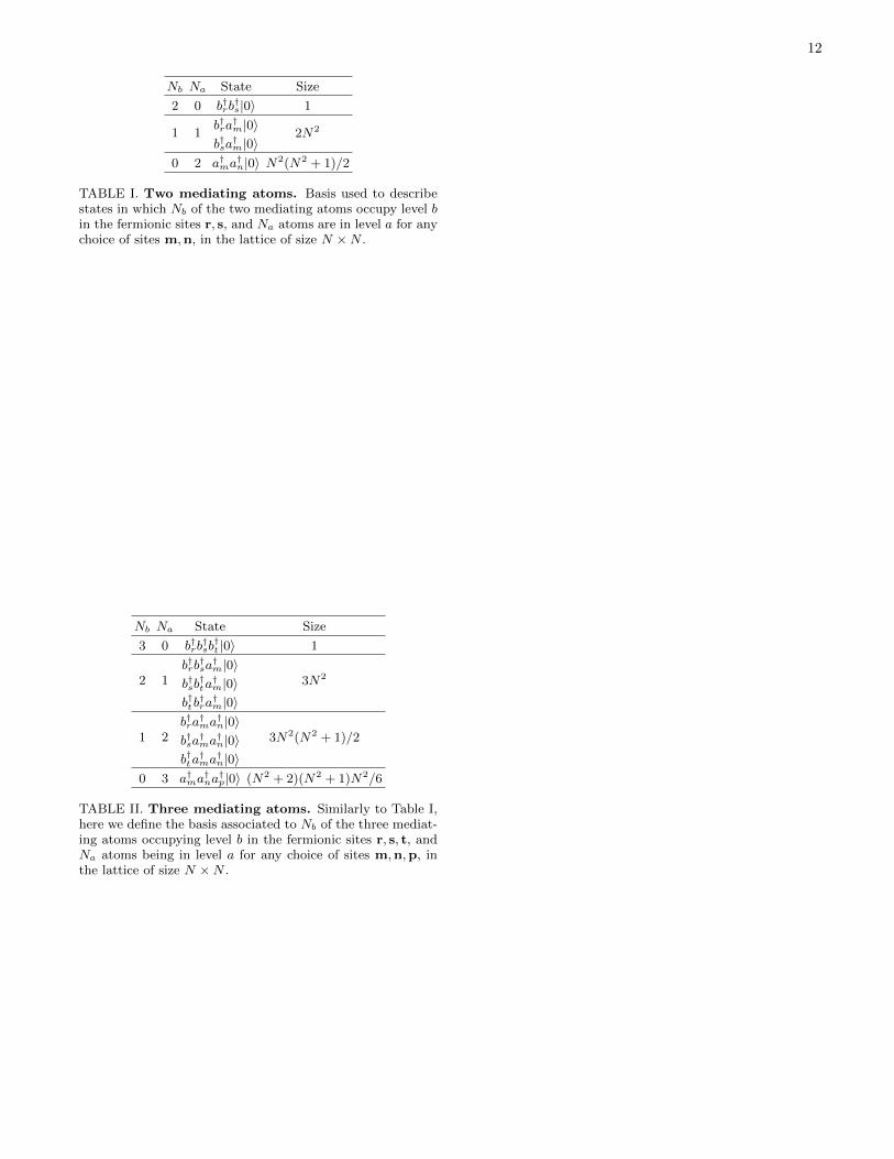
interact with the fermions, and |W/U | � 1, so that twomediating atoms in level b do not coexist in the samelattice site. For a configuration of 2 (3) fermions in sitesr, s(, t), and given the indistinguishability of the medi-ating atoms, we can further reduce the Hilbert space tostates written in the basis collected in Tables I and II.

Within this basis, in Fig. 4 we calculate how the energyof the bosonic ground-state energy E(d) depends on theirseparation d between two fermionic atoms fixed in latticesites [N/2−d/2, N/2] and [N/2+d/2, N/2], following thesame strategy used in the previous case for Nf = 2.

In the case Nf = 3, we observe that the biggest de-mand on computational memory corresponds to describ-ing processes in which the three mediating atoms simul-taneously populate the a-level. Such processes scale as[g/(U − δ)]6 in perturbation theory, and are subleadingwhen compared to the second-order terms. Therefore,truncating 0 ≤ Na ≤ 2 would allow to push the calcula-tion at a marginal error (see Table II).

To confirm this intuition, in Fig. S3(a) we use ITE tocalculate the bosonic bound state for 3 fermions describ-ing a triangular isosceles configuration. For moderatesizes (N = 16), we compare the numerical result givenby this truncated space to the one obtained for the totalbasis. As desired, we observe that (1) the truncation tothe space with up to 2 excitations in state a does notmodify the solution, and (2) the scaling is in agreementwith the calculation for a pairwise repulsion given by(C6).

12

Nb Na State Size

2 0 b†rb†s|0〉 1

1 1b†ra†m|0〉 2N2

b†sa†m|0〉

0 2 a†ma†n|0〉 N2(N2 + 1)/2

TABLE I. Two mediating atoms. Basis used to describestates in which Nb of the two mediating atoms occupy level bin the fermionic sites r, s, and Na atoms are in level a for anychoice of sites m,n, in the lattice of size N ×N .

Nb Na State Size

3 0 b†rb†sb†t |0〉 1

2 1b†rb†sa†m|0〉

3N2b†sb†ta†m|0〉

b†tb†ra†m|0〉

1 2b†ra†ma†n|0〉

3N2(N2 + 1)/2b†sa†ma†n|0〉

b†ta†ma†n|0〉

0 3 a†ma†na†p|0〉 (N2 + 2)(N2 + 1)N2/6

TABLE II. Three mediating atoms. Similarly to Table I,here we define the basis associated to Nb of the three mediat-ing atoms occupying level b in the fermionic sites r, s, t, andNa atoms being in level a for any choice of sites m,n,p, inthe lattice of size N ×N .