quantum mechanics || the formal framework of quantum mechanics

16. The Formal Framework of Quantum Mechanics

In this chapter we summarize the mathematical principles of quantum mechanics, using a more abstract mathematical formulation than before. Many of the relations which will be considered here have already been discussed in the preceding chapters in a more "physical" way and most have been proved in detail. Some of the explanations and proofs are supplemented or demonstrated once again in a more compact manner in additional exercises.

16.1 The Mathematical Foundation of Quantum Mechanics: Hilbert Space

By a Hilbert space H we mean an abstract number of elements, which are called vectors la}, Ib}, Ie} etc. H has the following properties:

1. The space H is a linear vector space above the body of the complex numbers /-L and v. It has three properties:

(a) To every pair of vectors la}, Ib}, a new vector Ie} is related, which is called the sum vector. It holds that

la} + Ib} = Ib} + la} (commutative law)

(Ia} + Ibn + Ie} = la} + (Ib} + len (associative law) . (16.1)

(b) A zero vector IO} exists, with the property

la} + IO} = la} . (16.2)

(c) To each vector la} of H, an antivector 1- a} exists, fulfilling the relation

la} + I-a} = IO} ;

for arbitrary complex numbers /-L and v, we have

/-L(la} + Ibn = /-L la} + /-L Ib} ,

(/-L+v) la} = /-L la} +v la} ,

/-LV la} = /-L(v lan,

lla} = la} .

(16.3)

(16.4)

W. Greiner, Quantum Mechanics© Springer-Verlag Berlin Heidelberg 2001

424 16. The Formal Framework of Quantum Mechanics

2. A scalar product is defined in the space H. It is denoted by

(Ja) , Jb)) or (aJb) ,

yielding a complex number. The scalar product has to fulfil the relations

(Ja) , A Jb)) = A(Ja) , Jb)) ,

(Ja) , Jb)+Jc)) = (Ja) , Jb))+(Ja), Jc)) ,

(Ja) , Jb)) = (Jb) , Ja))* .

The last equation may also be written as

(aJb) = (bJa)* .

It is easily shown from this, that

(A Ja) , Jb)) = A *(Ja) , Jb)) = A * (aJb) ,

and

follow. The norm of the vectors is defined by

IIJa) II = J(aJa)

(read: norm of vector Ja) = ,J(aJa)). It can be shown that Schwartz's inequality,

IIJa) II IIJb) II ~ J(aJb)J ,

is valid and that the equality is only valid for the case

Ja) = A Jb)

(parallelism of the vectors).

(16.5)

(16.6)

(l6.7a)

(16.7b)

6.8)

3. For every vector Ja) of H, a series Jan) of vectors exists, with the property that for every t: > 0, there is at least one vector Jan) of the series with

(16.9)

A series with this property is called compact, or we may say Jan) of the space H is separable.

16.1 The Mathematical Foundation of Quantum Mechanics: Hilbert Space

4. The Hilbert space is complete. This means that every vector la} of H can be arbitrarily exactly approximated by a series Ian}:

lim Ilia} -Ian} II = 0 . (16.10) n ..... oo

Then the series Ian} has a unique limiting value la}.

For Hilbert spaces with finite dimensions, axioms 3 and 4 follow from axioms 1 and 2; then 3 and 4 are superfluous. But they are necessary for spaces of dimension 00 that occur in quantum mechanics in most cases. In the following, we discuss once again some definitions that are used very often.

1. Orthogonality of Vectors:

Two vectors If} and Ig} are orthogonal if

{fIg} =0.

2. Orthonormal System:

The set {I fn} } of vectors is an orthonormal system if

{fnlfm} = onm .

3. Complete Orthonormal System:

(16.11)

(16.12)

The orthonormal system {Ifn}} is complete in H if an arbitrary vector If} of H can be expressed by

(16.13) n

In general, an are complex numbers:

am ~ (fmlf) ~ (1m ~>"1") = Lan {fmlfn}

n

=am , (16.14)

so that we can write

If} = L Ifn} {fnlf} (16.15) n

The complex numbers an are called the fn representation of If}; they represent, so to say, the vector If}; they are the components of I f} with respect to the basis {I fn} }. If the sum in the last equation encloses an infinite number of terms, then we speak of a Hilbert space of infinite dimensions. In quantum mechanics, this is usually the case.

425


16.2 Operators in Hilbert Space

A linear operator A induces a mapping of H upon itself or upon a subspace of H. Here,

A(a If) + fJlg) = aA If) + fJA Ig) (16.16)

The operator A is bounded, if

IIA 1f)11 s c 1I1f)11 (16.17)

for all I f) of H, C being the same constant for alII f). Bounded linear operators are continuous. This means that for

Ifn) -+ If) ,

A Ifn) -+ A If)

(16.18a)

(16.18b)

also follows. Two operators A and B are equal (A = B) if, for all vectors I f) of H,

A I f) = B If). (16.19)

The following definitions are often used:

(a) unity operator i : i If) = If)

(b) zero operator o : Olf) = 10) ;

(c) sum operator A+B (A + B) If) = A If) + B If)

(d) product operator AB : (AB) If) = A(B If) . (16.20)

The relations shown here have to be valid for all If) of H. With respect to the product operator, we have to add that, in general,

The commutator of A and B is defined by

[A, B]_ = AB - BA . (16.21)

Now we explain the very important concept of the adjoint of a restricted operator. If an operator A+ exists for the operator A for all If) and Ig) of H in such a way that

(Ig), A If) = (A+ Ig), If) , (16.22)

then A + is called the adjoint operator of A. This relation can also be expressed by

(16.23)

16.3 Eigenvalues and Eigenvectors

The adjoint of an operator (16.22) possesses the following properties, which are easily derived:

(1) (aA)+ = a* ,.1+ ;

(2) (A+B)+ = ,.1+ +B+ ;

(3) (AB)+ = B+ ,.1+

(4) (,.1+)+ = A . (16.24)

All these properties were discussed and proved in Chaps. 4 and 10. On the basis of the definition given above, the properties may immediately be confirmed.

An operator A fulfilling the relation

(16.25)

is called a Hermitian operator. From this it follows that the expectation values are real:

(1IAI/) = (1I A+I/)* = (1IAI/)* = real . (16.26)


We speak of an eigenvector la) of the operator A belonging to the eigenvalue a in the case

Ala) =a la) (16.27)

Here, the eigenvalue a is, in general, a complex number. Especially for Hermitian operators ,.1(,.1+ = A), the following is true.

(a) The eigenvalues of Hermitian operators are real. (b) If la' ) and la"), are two eigenvectors of a Hermitian operator A with two different eigenvalues a' =f:. a", then

(a'ia") =0 .

(c) The normalized eigenvectors of a bounded Hermitian operator A create a countable, complete orthonormal system. In this case the eigenvalues are discrete. Then we speak of a discrete spectrum.

We therefore can conclude that an arbitrary vector 11/1) may be expanded in terms of the complete orthonormal system la) of the Hermitian, restricted operator A:

11/1) = L la) (aI1/l) (16.28) a

427


As noted above, we have

(a'ia") = Oa'all • (16.29)

The scalar product of two vectors Icp} and Il{!} may be expressed in the A representation; also,

(cpll{!) = L (cpla) (all{!) . (16.30) a

Here, a helpful trick has been used. If we introduce the unity operator It, known as completeness, by

(16.31) a

we get

Il{!} = ill{!} = L la} (all{!) , (16.32) a

and, further,

(16.33) a

which is consistent with (16.28) and (16.30). The expansion (16.32) implies that

(16.34) a

Therefore we may also say that (all{!) is square-summable. Apparently the abstract Hilbert space is mapped onto the space of the square-summable functions (eigenfunctions of the operator A). This we call the A representation of l{! and mean the infinite set of numbers (all{!) in (16.32). Applying an operator B to Il{!} yields

(16.35) a"

Thus the operator B can be written in the A representation as the matrix

(aIIBlaz) (azIBlaz)

(16.36)


and the vector t in A representation as

It} --+ (a'it) = (16.37)

Therefore the operator B in A representation is a quadratic matrix; the vector It}, a column matrix. The operator A itself is given in the A representation of its eigenrepresentation as

(a'IAla") = a'oala" . (16.38)

Sometimes it is advantageous to write the (arbitrary) operator B in the form

B = iBi = L la'){a'IBla") (a" I . (16.39) a',a"

The analogy of the representation of a vector in a Hilbert space to the components of a vector in vector space is evident. The choice of the representation coincides with the choice of the coordinate system in the Hilbert space.

Now we proceed to the transformation of the A representation into B representation. Here, the so-called transformation matrix

(alb)

plays an important role. In analogy to (16.38) it follows that

(b'l Bib") = b'Oblb" .

It is convenient to start from the unity operator

Ii = L lal){all = L!h')(b'l . a' b'

The following relations can be understood immediately:

(b'lt)=(b'lilt)= L(b'la')(a'lt) , a'

(a'it) = (a'lilt) = L (a'lb'){b'lt) , b'

(b'lelb") = (b'lielLlb") = L (b'la') (a'iCia") (a"!h")

Similarly to (16.42), we get

(a'l Bela") = (a'IBiela") = L (a'l B la"')(a'" lela") . a'"

(16.40)

(16.41)

(16.42)

(16.43)

(16.44)

429


This means that for the matrix element of the product of two operators Ii C, the customary rules for matrix multiplication are valid.

EXERCISE

16.1 The Trace of an Operator

Problem. Show that the trace of an operator is independent of its representation.

Solution. The trace l of the operator C in the A representation is

trC = L (a'ICla') . a'

Then we write

trC = L (a'ICla') ... = triCi a'

= L L L (a'jb') (b'IClb") (b"la') a' b' bl!

a' b' bl!

b' bl!

= L(b"licjb") = L{b"lcjb") . bl! bl!

Since Cle) = ele), we have in the eigenrepresentation of C

trC = L (e'ICle') c'

= Le' (e'le') = Le' . c' c'

1 The German name for trace, "Spur", is often used in the literature.

16.4 Operators with Continuous or Discrete-Continuous (Mixed) Spectra

EXERCISE

16.2 A Proof

Problem. Show that

L L l(a'lcla"W = trCC+ a' a"

Solution. It can easily be seen that

LL l(a'lcla"W = LL(a'lcla"}(a'ICla"}* a' a" af aff

= L L (a'ICla"}(a"IC+la') a' a"

= L (a'ICC+la') = trcc+ a'

Here we have used (16.23) and (16.44).

16.4 Operators with Continuous or Discrete-Continuous (Mixed) Spectra

Many operators occurring in quantum mechanics do not have a discrete, but a continuous or a mixed (discrete-continuous), spectrum. An example of an operator with a mixed spectrum is the well-known Hamiltonian of the hydrogen atom. Actually all Hamiltonians for atoms and nuclei have discrete and continuous spectral ranges; therefore they have mixed spectra. Usually the discrete eigenvalues are connected with bound states and the continuous eigenvalues are connected with free, unbound states. The representations related to such operators cause some difficulties because, for continuous spectra, the eigenvectors are not normalizable to unity (cf. our discussion of Weyl's eigendifferentials in Chaps. 4 and 5).

1. Operators with a Continuous Spectrum

The operator A has a continuous spectrum if the eigenvalue a in

Ala) = ala) (16.45)

431

432

a

a ···,

Fig. 16.1. A mixed spectrum. For a < ii, the spectrum is discrete; for a > ii it is continuous


is continuous. The states la} can no longer be nonnalized to unity, but must be nonnalized to Dirac's delta function:

(a'la") = 8(a' - a") . (16.46)

Here, the delta function replaces, so to speak, Kronecker's 8 of the discrete spectrum [cf. (16.29)]. In the expansion of a state Iv} in tenns of a complete set la}, the sums [cf. (16.28)] are replaced by integrals:

Iv} = f la')(a'lv) da' . (16.47)

(a' Iv) represents the wave function in the A representation. The inner product of two vectors I(j]} and Iv} changes analogously to (16.30) into

(16.48a)

which is sometimes written as

((j]lv) = f (j]*(a')v(a')da' . (16.48b)

Here, v(a) = (alv) may be understood (somewhat imprecisely) as a "wave function in A space". Of course, it is just the A representation of Iv}.

2. Operators with a Mixed Spectrum

If the equation

Ala} =a la}

yields discrete as well as continuous eigenvalues a, we are dealing with a mixed spectrum (cf. Fig. 16.1).

In these cases, the expansion of Iv} in tenns of la} reads

Iv} = L la')(a'lv)+ f la') (a'lv) da' , a'

(16.49)

where the sum extends over the discrete, and the integral over the continuous, eigenstates la}.

In order to make the notation more compact, it is understood that La' or J ... da' is split into the discrete and the continuous parts of the spectrum, if there are any, according to (16.49).

16.5 Operator Functions


Operator functions f(A) may be defined as a power series if the function f(x) can be expanded in this way. Thus if

00

f(x) = L Cnxn , n=O

then the operator function f(A) is defined by

00

f(A) = L CnAn . (16.50) n=O

For example, eA, cos A, etc. may be defined in this way. Another possibility of defining operator functions is obtained via their eigenvalues: if

Ala'} = a' la'} ,

then we have

f(A) la'} = f(a') la'} (16.51)

For operator functions of the fonn (16.50), (16.51) follows immediately. Two exercises will illustrate these points.

EXERCISE


Problem. Derive the relation

WI f(A) Ib"} = L (b'la') f(a') (a'jb") a'

Solution. We calculate:

(b'l f(A) Ib"} = (b'l if(A)i Ib")

= L (b'la') (a'lf(A) la"} (a"jb") a',a"

= L (b'la') f(a')oa',a" (a"jb") a'.a"

= L (b'la') f(a') (a'jb") (1)

a'

433


EXERCISE

16.4 Power-Series and Eigenvalue Methods

Problem. Show by the method of power-series expansion (16.50) and by the method of eigenvalues (16.51) that

ei (f312)o-x = cos 2 1 Slll 2 ( f3 .. f3)

i sin ~ cos ~

if

Solution. (a) We use the power series of the exponential function and get

(1)

We have u; = 1 = (~ ~) and therefore u; = u x. For this reason, the series (1)

splits into even and odd powers. We get

ei (f312)o-x = 1 t ~! c;r +ux L ~! c;r n even n odd

1 fJ . . fJ = cos 2 + lUx slll2 . (2)

(b) We use the method of eigenvalues (16.51). It is suitable to introduce the vectors

Iz, +1) = (~) and Iz, -1) = G) , (3)

i.e. the eigenstates of U z = (~ ~ 1). This property is expressed by the notation

Iz, )..). Now, it can easily be checked that

(ZiluxIZj)=(~ ~) . (4)

To use the method of eigenvalues, we need the eigenvalues of Ux . For this purpose, we solve the eigenvalue problem

Ux Ix, )..) =).. Ix,)..) , (5)


and find A = ± 1 and the normalized eigenvectors,

Using (1) of Exercise 16.3, we get

(z, i I eiC{Jf2)ux Iz, j) = L (z, ilx, A) eiC{Jf2»)' (x, Alz, j) ).=±1

(6)

(7)

From this we are able to construct all matrix elements. For example, for i = j = 1, we get

0) G) eiC{3/2) ~ (1 1) (b) + _1 (1 0) ( 1 ) e-iC{3/2)_1 (1

.,fi -1 .,fi

= ~ ei({3/2) + ~ e-iC{3/2) = cos ~ . 222

-1) (b)

In a similar manner we derive the other matrix elements, and finally arrive at

( t!. .. t!.) . cos 2 1 sm 2

(z, i I e1C{3/2)ux Iz, j) = . . . 1 sm t!. cos t!. 2 2

(8)

Even the inverse operator A -1 can be defined by the method of eigenvalues (and not only by the inversion of the matrix), namely:

A-I la'} = ~, la'} . (16.52)

With Ala'} = a'la'), we have

If one of the eigenvalues of A, i.e. one of the quantities a', vanishes, the inverse operator cannot be defined. In this case, A-I does not exist.

435

Exercise 16.4


16.6 Unitary Transformations

An operator (; is unitary if

(;-1 = (;+ . (16.53)

A unitary transformation is given by a unitary operator:

(16.54)

Hence, for an operator, it follows that

( f I A I") (A f I A I A ") (f I A+ A AI") anew Anew anew = Uaold Anew Uaold = aold U AnewU aold

def (f I A I") == aold Aold aold .

Therefore A A+ A A

Aold = U AnewU, or A A+ -I A A_I A A A+

Anew = (U) AoidU = U AoidU , (16.55)

where we have used (16.53). It can easily be checked that scalar products are invariant under unitary transfonnations, because

(16.56)

Also the eigenvalues of Anew are the same as those of AOld (invariance of the eigenvalues), i.e.

A If) A A A + A I Af) A A If) A f If) Anew anew = U Aold~ aold = U Aold aold = Uaold aold

n

It can easily be shown that, given

Cold = AoldBold and

bOld = AOld + BOld ,

it also holds that

C new = AnewBnew and

bnew = Anew + Bnew .

(16.57)

(16.58)

(16.59)

(16.58a)

(16.59a)

The generalization of these relations is obvious: All algebraic operations remain unchanged by unitary transformations.

16.7 The Direct-Product Space

16.7 The Direct-Product Space

Frequently the Hilbert space must be expanded, because new degrees of freedom are discovered. One example we have already encountered is the spin of the electron (see Chap. 12). The total wave function consists of the product of the spatial wave function 1f.r(x, y, z) and the spin wave function x(a):

1f.r(x, y, z) X (a) .

We say the Hilbert space is extended by direct-product formation. The following examples explain this further.

A nucleon may be either a neutron or a proton with nearly identical masses: mpc2 = 938.256 MeV, mnc2 = 939.550 MeV. For this reason we consider it as a particle with two states, the proton state Ip) and the neutron state In):

(1) Ip) = , o charge

In) = (0) 1 charge

(16.60)

The vectors Ip) and In) span the two-dimensional charge space or isospin space (in analogy to the spin). Since the nucleon may also occupy two different spin states

It) = (1). and o spm It) = (~) . '

spm (16.61)

the direct product space consisting of spin and isospin space is given by the fourdimensional space with the basis vectors

110 (1) Ip t) = x = 0 ' (ot ... (ot 0

1 ° 1 (0) Ip t) = x = ° ' (ot,.. Ct 0

° 1 0 (0) In t) = x = 1 ' Ct." (ot 0

o 0 0 (0) In t) = x = 0 . Ct.,.. Ct 1

(16.62)

437


Thus, in this four-dimensional space, the charge properties as well as the spin properties of the nucleon can be described. If further "intrinsic" properties (i.e. more inner degrees of freedom) of the nucleon should be discovered, the space will have to be further enlarged. In fact, a situation similar to the one just discussed arises if we consider particles and antiparticles.2

16.8 The Axioms of Quantum Mechanics

It is not easy to summarize the axioms or rules of quantum mechanics. Here we will follow E.G. Harris3 and refer to the extensive discussions of von Neumann4

and Jauch.5 Quantum mechanics is based upon the following correspondence between

physical and mathematical quantities.

1. The state of a physical system is characterized by a vector (more precisely, by a vector beam) in Hilbert space. Hence, I1/!} and AI1/!} describe the same state. In general, the state vectors are normalized to unity, to enable the interpretation of probability.

2. The dynamic observable physical quantities (observables) are described by operators in the Hilbert space H. These operators of observables are Hermitian operators. Their eigenvectors form a basis of H; any vector of H may be expanded in terms of this basis.

These general principles are supplemented by the following fundamental physical axioms.

Axiom 1: As a result of the measurement of an observable, only one of the eigenvalues of the corresponding operator can be found. After the measurement, the system occupies that state which corresponds to the measured eigenvalue.

Axiom 2: If the system occupies the state la'}, the probability of finding the value b' in a measurement for Breads

W(A', B') = 1 (a'ih') 12 . (16.63)

2 We will encounter this situation in W. Greiner: Relativistic Quantum Mechanics, 3rd ed. (Springer, Berlin, Heidelberg 2000), where the Dirac spinor also turns out to have four components: two for the spin and two for the particle-antiparticle degrees of freedom.

3 E.G. Harris: A Pedestrian Approach to Quantum Field Theory (Wiley, New York 1972). 4 J. von Neumann: The Mathematical Foundations of Quantum Mechanics (Princeton,

NJ 1955). 5 J.M. Jauch: Foundations of Quantum Mechanics (Addison-Wesley, Reading, MA

1968).

16.8 The Axioms of Quantum Mechanics

If B has a continuous spectrum,

dW(A', B') = 1 (a'lb)' 12 db' (16.63a)

is the probability that B has a value within the interval between b' and b' + db'.

Axiom 3: The operators A and B, which correspond to the classical quantities A and B, fulfil the commutation relation

[A, B]_ = AB - BA = in{A, B}op , (16.64)

where {A, B}op is the operator which corresponds to the classical Poisson bracket,

(16.65)

qi and Pi are the classical coordinates and momenta of the system. It follows that

(16.66)

and, similarly, for the orbital angular momentum,

i = r x p = (ypz - ZPy, zPx -xpz, XPy - YPx) ,

A A 'f; ~ (OLx oLy oLx OL y ) [Lx,Ly]_=ln~ -----

i oqi 0Pi 0Pi oqi op

= ih[( - Py)( -x) - (Y)(Px)]op

= in (xPy - YPx) = ini z . (16.67)

For the other angular-momentum commutation relations we get a similar result and may write

(16.68)

We should pay attention to the following consequence of this axiom. If we define the expectation value of an observable A by

(16.69)

and the uncertainty (the mean variation) by

(16.70)

it follows that (see Sect. 4.7)

(16.71)

439


This is the general formulation of Heisenberg's uncertainty relation. In particular, for the variables Pi and % using (16.66) we have

n I::!.p.l::!.q. > -8·· I J - 2 IJ • (16.72)

Hitherto, we have dealt with states (vectors) and observables at one instant of time. The dynamics of a system may be described in different, equivalent ways. The most customary one is the Schrodinger picture, in which the state vector is time dependent, but the operators of the observables are independent of time.

Axiom4: If a system is described by the state l1/!to} at time to and by l1/!t} at time t, both states are connected by the unitary transformation

(16.73)

where

~ [ 1 ~ ] U(t-to) =exp -"h,H(t-to) (16.74)

and H is the Hamiltonian of the system. Schrodinger's equation follows from (16.73) and (16.74). Let

dt = t -to

then

n a ~ --:--I1/!} = HI1/!}

1 at

~ i ~ and U(dt) = 1- "h,Hdt ;

(16.75)

Notice that Schrodinger's equation is generally valid. In particular, it is valid for time-independent, as well as for time-dependent, Hamiltonians iI. Only in the first case (H time independent) may we conclude (16.73) from (16.75) (cf. Chap. 11). Therefore the special form of the time development (16.73) is only valid for time-independent Hamiltonians.6

The Heisenberg picture is another description of the dynamics of a physical system, which is equivalent to the SchrOdinger picture, as mentioned above. We obtain it from (16.73), by applying the unitary transformation

(16.76)

6 See W. Greiner, B. MUller: Quantum Mechanics - Symmetries, 2nd ed. (Springer, Berlin, Heidelberg 1994), especially the section on isotropy in time.

16.9 Free Particles

to the state vectors. Then the operators transform according to (16.55), and we get

(16.77)

The subscripts Hand S stand for "Heisenberg" and "SchrMinger", respectively. In Heisenberg's representation, the state 11/1r)H = lo/to)8 is apparently a fixed time-independent state. Compared to this, the operators

(16.78)

are time dependent because of(16.77) and (16.74). By differentiation of (16.78), we find that AH(t) fulfils the equation

na ~ ~ ~ ~~ ~ ~ --;--a AH = AHH - HAH = [AH, H1-

1 t (16.79)

It is called Heisenberg's equation o/motion for the operator AH in the Heisenberg picture and has to be considered in analogy to the classical equation of motion of a dynamic variable A in the form of Poisson brackets,

dA - ={A,H}. dt

(16.80)

Heisenberg's equation leads immediately to the important result that an operator which commutes with the Hamiltonian is a constant of motion.

16.9 Free Particles

It will be useful to study the motion of a free particle more carefully and to systematically summarize the various mathematical operations and tricks once again. First we consider the free motion of a particle in one dimension and later we will devote ourselves to the three-dimensional problem. The dynamic variables are now the coordinate x, the momentum p, and the Hamiltonian is iI = jJ2/2m. The eigenvalue equations for x and p read

x Ix'} = x' Ix'} , jJ IP'} = p' IP'} .

(16.81a)

(16.81b)

By definition, a truly free particle may occupy any position x' and also have any momentum p'. Therefore in (16.81) we have to deal with continuous spectra, so that the eigenstates Ix') and Ip') must be normalized to 8 functions

(x' Ix"} = 8(x' - x") , (p'IP") = 8(p' - p") .

(16.82a)

(16.82b)

441


Using the commutation relation

[x,pl-=xp-jJX=inl,

we can calculate the matrix elements of p in x representation:

(x'lxp - pxlx"} = (x'IHp - plXlx"}

= f dxlll[(x'ix IXIll}(XIllI pix"} - (x'lplxlll }(xlll lxlx"}l

= f dxlll [XIll8(x' -xlll)(x"'lplx"}

-(x'lplxlll }x"8(x" -x"')]

= x'(x'lplx"} -x"(x'lplx"} = (x' -x")(x'lplx"} .

On the other hand, because of (16.83),

( 'I ~ ~ ~ ~ I"} . ~ ~(' ") x x P - px x = 11£0 X - X ,

so that

(x' -x")(x'lplx"} = in8(x' -x") .

With the aid of the identity

d x dx 8(x) = -8(x) ,

we get

in8(x' - x") = -in(x' - x") a 8(x' - x") a(x' - x")

.~(' ,,)a8(x' -x") =-11£ x-x ax'

Finally, by using (16.86), we obtain

(x'lplx"} = -in a:,8(X' -x") .

In the following exercise we will recalculate the analogous relation

(p'lxlp"} = in a~,8(P' - p") ,

(16.83)

(16.84)

(16.85)

(16.86)

(16.87)

(16.88)

(16.89)

(16.90)

which is what we expect, because of the antisymmetric position of x and p in (16.84).

16.9 Free Particles

EXERCISE

16.5 Position Operator in Momentum Space

Problem. Prove the relation

in a similar manner to relation (16.89).

Solution.

(p' Ix p - Pi I P") = (p' lit P - plX I P")

= f dp"'[(p' Ix Ip"') (p'" IplP") - (p'l plP''') (P'''lxlP'')]

= f dp"'[p"8(p" - p"')(p' Ix IP''') - p'8(p'" - p')(p"'lxlp")] = (p" - p')(p'lxlP")

and, on the other hand, because of (16.83), this is equal to

in8(p' - p") .

So we get

- (p' - p")(p'lxlp") = in8(p' - pI!)

= -in(p' _ pI!) a 8(p' _ p") a(p' - p")

• J< (' ") a ~(' ") = In p - p -u p - p . ap'

It follows that

[according to (16.87)]

(1)

(2)

(3)

(4)

(5)

443


The matrix elements (x'lp2Ix") can also be calculated directly by computing the matrix product. Briefly,

(X'lp2Ix") = (x'lplplx") = f dx"'(x'lplx"'}(xllllplx"}

= f dx lll [-ili~8(X' -xII!) (-ili-a-8(xlll -x"»)] ax' axlll

= -ili~ f dx"'8(x' -x"') (-ili-a-8(X'" -x"») ~, ~'"

( • t; a)2 , " = -In- 8(x -x ) .

ax'

Similarly, we get the more general relations,

(x' I pn Ix") = (-iii a~' ) n 8(x' - x") and

(p'lxn Ip") = (iii a:') n 8(p' - p") .

(16.91)

(16.92)

(16.93)

Now we consider the eigenvalue problem for the momentum in coordinate representation:

piP'} = p' Ip'} (16.94)

We have

(x'lplP') = f dx"(x'lplx"} (x"IP') = f dx" (-iii a~,8(X' -x"») (x"lp')

= -iii a~' f dx" 8(x' - x") (x"ll)

= -iii a~' (x'IP') . (16.95)

On the other hand, it follows from (16.94) that

(x'lpll) = p' (x'll) ,

so that the differential equation for (x'IP'),

-iii a~' (x'll) = p' (x'll) , (16.96)

results. Its solution is

( 'I ') , 1 (i, ') x p == 1/1 pi (x ) = ~ exp ~ p x v2nli n

(16.97)

16.9 Free Particles

Here, we have chosen the normalization in such a way that

(P"IP') = f dx' (P"lx') (x'IP')

= f dx'1/t;,,(x')1/tp,(x') = 8(p" - p') . (16.98)

Now we generalize the above results to three dimensions. According to (16.66), the three space coordinates commute with each other. Hence, they may be combined into the state

Ix} = Ix, y, z} . (16.99)

By definition Ix} is also an eigenstate of the operators X, y and z:

X Ix'} = x' Ix'}, y Ix'} = y' Ix'}, z Ix'} = z' Ix'} ,

or, in short,

X Ix'} = x' Ix'} (16.100)

As the spectrum is continuous, we may (must) normalize to 8 functions:

(x"lx') = 8(x' - x") = 8(x' - x")8(y' - y")8(z' - Zll) . (16.101)

The operators Px, py, pz commute with each other, too, so that we may form the common eigenvector Ip} with

ft Ip'} = p' IP'} . (16.102)

Again, we have normalization to 8 functions:

(piliP') = 8(p' - p") = 8(p~ - p~)8(p~ - p~)8(p~ - p~) . (16.103)

Now we want to return to (16.89). Every single step which led to this solution may be repeated for each component Px, py, pz with the state vector Ix}. Thus we get

(x'IPxlx") = -iii a~,8(X' -x")

etc.

We may combine this in the form

(x'lftlx") = -iii a~,8(X' -x")

== -iii (a~' 8 (x' - x") , a -8(x' -x")

ay' '

(16.104)

(16.105)

~8(x' - XII») . az'

445

446 16. The Fonna} Framework of Quantum Mechanics

Similarly, we conclude immediately that

(p'lill') = in a:,8(P' - p")

.~ (a , " = In [il8(p - P ) , px

a [il8(P' - p") ,

py

(16.106)

a;~ 8(p' - P")) , which is analogous to (16.90). The differential equation (16.96) can also be generalized to three dimensions without any difficulties:

-in a~' (x'll) = p' (x'll) , (16.107)

with the solution

( 'I ') , I (i , ') x p = 1fJp'(x) = (271n)3/2 exp "h,P'x , (16.108)

normalized to 8 functions. Using the results (16.91) and (16.92), we get the Hamiltonian of a free particle H = fi2/2m in x representation:

(x'IHlx") = (x' I :~ I x") = - ~~ V 28(x' -x") . (16.109)

In p representation, this reads

(p'IHlp") = (l I :~ I p") = (~~2 8(p' - p") . (16.110)

Now we turn to the time-dependent description. In particular, we are interested in the propagation of the wave which describes a free particle; this is calledfree propagation. For this, we use (16.73) and (16.74), and express 1fJ(x', t) = (x'l1fJt) by 1fJ(x', to) = (x'l1fJto) as

l1fJt) =exp[-iH(t-to)/n] l1fJto) ,

1fJ(x', t) = (x'l1fJt) = (x'i exp[ -iH(t - to) In] l1fJto)

= f d3x"(x'l exp[ -iH(t - to)/n] Ix") (x"l1fJto)

= f d3x"G(x', tlx", to)1fJ(x", to) . (16.111)

Here,

G(x', tlx", to) = (x'i exp[ -iH(t - to)ln] Ix") (16.112)

is called Green's function or the propagator. It describes the time development of the wave 1fJ(x', t), starting with the initial waves 1fJ(x", to) . Its explicit calculation

16.9 Free Particles

can be accomplished immediately in the case of free particles with Ii = p2/2m :

G(x', tlx", to) = f f d3 p' d3 p" (x'll)

x (p' lexp [ -k ;~ (t - to) J I pll) (p"lx")

= f f d3 p' d3 p" (x'lp')exp [ -k ~: (t -to) J X 8(p' - p") (plllx")

(16.113)

f d3 p' { i [ p'2 J } = --- exp - p'. (x" -x') - -(t - to) (21Tn)3 n 2m

The integral can be computed analytically (cf. Exercise 16.6), giving

[ m J3/2 rim (x" -X')2J G(x'tlx"to) = exp - . 21Tin(t - to) 2n t - to

(16.114)

Finally, we want to make some comments on the description of free particles with spin. This is simply done by constructing the direct product of a vector Ix'), Ip} or I1/!} and a spin vector la}. For particles with spin 1/2, the vector la} is, for example, given by

Iz, t} = (~), Iz, *} = G) . (16.115)

The argument z of these s\in vectors indicates that we have chosen the represen

tation with az = (~ ~ 1) being diagonal. Hence, we have

11/!, a} = I1/!} la} and (16.116)

(xl1/!, a) = 1/!(x) la) = ( 1/!1 (X)) 1/!2(X)

(16.117)

Thus a spin-l /2 particle is represented by a wave function with two components (a spinor).

447


EXERCISE

16.6 Calculating the Propagator Integral

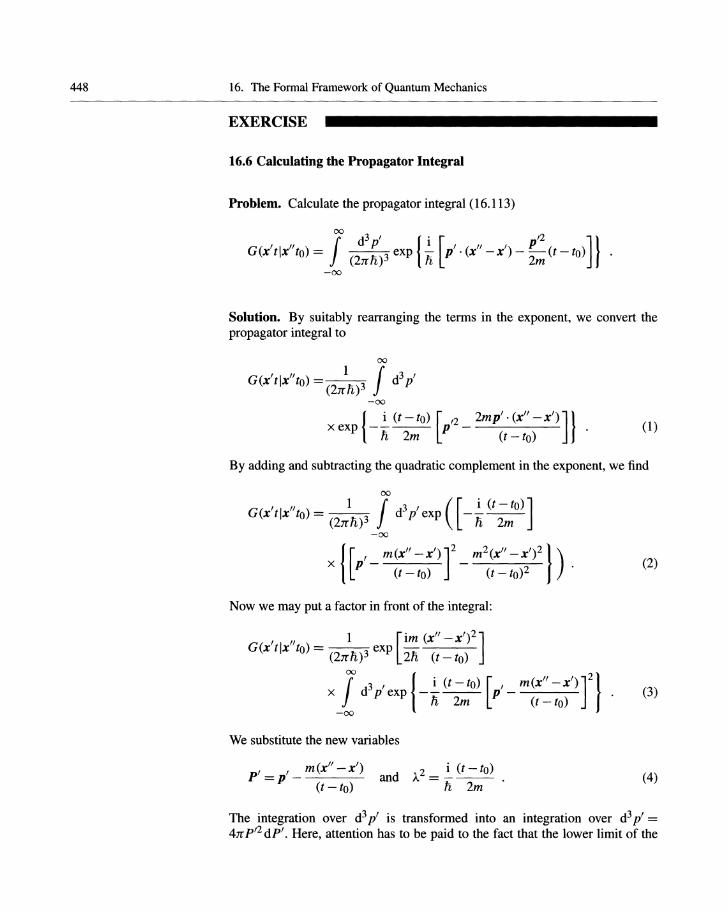
Problem. Calculate the propagator integral (16.113)

00

G(x' tlx" to) = / d3 P' exp {~ [p' . (x" _ x') _ p,2 (t - to)] } (2:rrn)3 11, 2m

-00

Solution. By suitably rearranging the terms in the exponent, we convert the propagator integral to

00 , " If 3 , G(x tlx to) d (2:rrn)3 P

-00

{ i (t - to) ['2 2mp'· (x" -X')]} x exp ----- p -n 2m (t - to) (1)

By adding and subtracting the quadratic complement in the exponent, we find

,,, 1 /00 3, ( [ i (t - to) ] G(x tlx to) = (2:rrn)3 d p exp -1i~

-00

x I[p'- m(x"-x')]2 - m2(x"-x')2\) (t - to) (t - to)2

Now we may put a factor in front of the integral:

1 [im (x" _X')2] G(x'tlx"to) = ~ exp t;"---

(2:rrn) 2n (t - to)

/00 d3, I i (t - to) [, m(x" - x') ]2\ x p exp ----- p -----

11, 2m (t -to) -00

We substitute the new variables

m(x" -x') p'=p'----

(t - to)

(2)

(3)

(4)

The integration over d3 p' is transformed into an integration over d3 p' = 4:rr p,2 dP'. Here, attention has to be paid to the fact that the lower limit of the

16.9 Free Particles

integral becomes zero:

4Jr [ m (x" - x')2 ] G(x'tlx"to) = (2Jrn)3 exp i 2n (t-to)

00

x f dP' p'2 exp( _).. 2 p,2) (5)

o

Because 00

f dx 2 _a2x 2 v'1i x e = 4a3 ' (6)

o

we get immediately

( m )3/2 (im (x" _X')2) G(x'tlx"to) =. exp -----

2Jrln(t - to) 2n t - to (7)

EXAMPLE

16.7 The One-Dimensional Oscillator in Various Representations

The harmonic oscillator plays an important role in many areas of physics; above all, in field theory (e.g. quantization of the electromagnetic field). Thus it is useful to summarize its properties. The Hamiltonian of the one-dimensional oscillator is given by

A A A 1 A2 mw2 A2 H(x,P)=2m P +-2-x ,

and the corresponding energy eigenvalue problem reads

HIE) = EIE) .

We solve the problem (2) for different representations.

(a) x Representation (Coordinate Representation)

Here, H may be written as [cf. (16.91) and (16.92)]

(x'i H Ix") = H (x', p')8(x' - x")

= H x - - 8(x - x ) A(,no) , /I

, i ox' '

(1)

(2)

(3)

(4)

449

Exercise 16.6

450

Example 16.7


Now (2) reads

(x'IIiIE) = f dx"(x' I Ii Ix"} (x"IE)

= f dx" Ii (X', ~ a~' ) 8(x' - x") (x"l E)

= Ii (x', ~ a~') (x'IE) = E (x'IE) . (5)

In the last step, we have written down the right-hand side of (2). Using 1/IE(X') = (x'IE), we may write

~(,na), , H x, T ax' 1/IE(X) = E1/IE{X) . (6)

This differential equation, familiar from Chap. 7, has usable solutions only if E adopts the eigenvalues

En = nw(n +~), n = 0,1, 2, ... ,00 .

The solutions belonging to these eigenvalues are

1/IE (x') = - --Hn(~)e-(~ /2) , ( mW)1/4 1 2

n rrn v'2nn!

with ~ = -/mwjnx'. Hn (~) are the well-known Hermite polynomials.

(b) p Representation (Momentum Representation)

(7)

(8)

Because of(16.81b) and (16.93), the Hamiltonian (1) in p representation is given by

( , I ~ I") ~ , , " p H p = H(x, p )8(p - p )

~ ( n a ,) , " =H -Tap"P 8(p -p), (9)

where

Ii (_~~ ,) __ 1_ '2_ mw2 n2~ i a p' , p - 2m p 2 a p,2 . (10)

Then, with (p'IE) = 1/IE(p'), (2) reads

(p'IIiIE) = f dp"(P' I Ii I P"} (p"IE)

= f dp" Ii (-~ a:' , p') 8{p' - p") (P"IE)

~ ( n a ,) , =H -Tap' ,p 1/IE{p)

= E1/IE{p') . (11)

16.9 Free Particles

In the last step we added the right-hand side of (2). The resulting eigenvalue equation in momentum space,

( mu}ti2 a 1 12) I I

--2- ap'2 + 2m p o/E(p) = Eo/E(p) , (12)

is easily transformed into

( ti 2 a2 1 12) , E I

--2 a 12 + -2 3 2P o/E(p) = 2:2o/E(p) , m p mw mw (13)

( _ ti2 ~ + mil} p12) o/E(p') = Eo/E(p') . 2m ap,2 2

(14)

Here, we have set il} = 1/ m4 w2 and E = E / m 2 w2 . Equation (14) is identical to (4) and (6). Thus the eigenvalues are

- - 1 En = tiw(n + 2)' n = 0, 1, ... ,00

or

(15)

Thus they are identical to the values we got in (7). In the same easy way, (8) is transformed into the wave function o/En (pi) in momentum space:

(16)

According to Axiom 2 [see (16.63) and (16.63a)], the probability of finding a particle in the energy state 0/ En (X') in the interval between x' and x' + dx' is given by

(17)

In the same manner, the probability of finding the particle with a momentum between pi and p' + dp' can be calculated:

(18)

The wave functions in coordinate space o/En (x') and in momentum space o/En (pi) are connected by

(xii En} = o/En(X' ) = f dpl(x'lp'}(P'IEn}

f dp' (i ) = ,.j21!ti exp 1i pi x' o/En (P') (19a)

451

Example 16.7

452

Example 16.7

16. The Fonnal Framework of Quantum Mechanics

and

o/En(P') = f J::n exp (-kp'x') o/En(X') , (l9b)

respectively.

(c) Algebraic Method (Algebraic Representation)

The algebraic method does not explicitly use any representation to solve the eigenvalue problem (2); it is particularly useful in field theory. We introduce the operators

(20a)

and

A+ Jmw A i A a = -x- p. 211, J2mnw

(20b)

They are called the annihilation operator (0) and the creation operator (0+), respectively, of oscillator phonons.1t can be seen that (0)+ = 0+; i.e. 0 = (0+)+. Their commutation relations are easily calculated:

and

In a similar manner, we find 2 .

A+ A mw A2 pIA A A A

a a= 2n X +2mnw +2n(xP-px) 1 A 1 = -H--' thus

nw 2 ' A A+ A 1 A 1

H = nw(a a+ 2:) = nw(N + 2:)' where

N=o+o.

We denote the eigenvectors of IV by In}, so we have

N In} = n In} .

(22)

(23)

(24)

(25)

We study the vector Ig}, which results from applying the annihilation operator 0 to In}:

Ig} = 0 In} . (26)

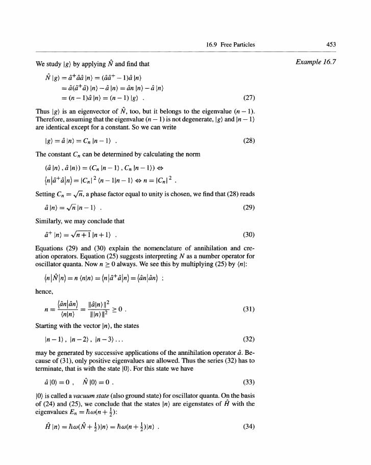
We study Ig) by applying fl and find that

fl Ig) = a+ aa In) = (aa+ -1)a In) =a(a+a) In) -a In) =an In) -a In) = (n -1)a In) = (n -1) Ig) .

16.9 Free Particles

(27)

Thus Ig) is an eigenvector of fl, too, but it belongs to the eigenvalue (n -1). Therefore, assuming that the eigenvalue (n -1) is not degenerate, Ig) and In - 1) are identical except for a constant. So we can write

Ig) = a In) = Cn In -1) .

The constant C n can be determined by calculating the norm

(a In), a In)) = (Cn In -1) ,Cn In -1)) -¢>

(nJa+aJn) = ICn l2 (n -lin -1) -¢> n = ICn l2 .

(28)

Setting Cn = yn, a phase factor equal to unity is chosen, we find that (28) reads

a In) = In In -1) .

Similarly, we may conclude that

a+ In) = -In+l" In + 1) .

(29)

(30)

Equations (29) and (30) explain the nomenclature of annihilation and creation operators. Equation (25) suggests interpreting N as a number operator for oscillator quanta. Now n :::: 0 always. We see this by multiplying (25) by (n I:

(nJflJn) = n (nln) = (nJa+aJn) = (anJan)

hence,

(an Jan) IIaln) 112 n=---= >0.

(nln) IIln)II2 -(31)

Starting with the vector In), the states

In - 1), In - 2), In - 3) ... (32)

may be generated by successive applications of the annihilation operator a. Because of (31), only positive eigenvalues are allowed. Thus the series (32) has to terminate, that is with the state 10). For this state we have

(33)

10) is called a vacuum state (also ground state) for oscillator quanta. On the basis of (24) and (25), we conclude that the states In) are eigenstates of iI with the eigenvalues En = 'fiw(n + i):

(34)

453

Example 16.7

454

Example 16.7


Frequently the matrix elements of i and p have to be determined. They are easily specified by solving (20) for i and p, respectively:

A r;r; A+ A x= --(a +a), 2mw

A .JmnW(A+ A) p=l --a -a , 2

and, by using (29) and (30),

(nlliln2) = J n [Jn2 + 18n[ n2+1 + .fi1i.8n[ n2-1] , 2mw ' ,

(nllpln2) = iJm~w [Jn2 + 18n[,n2+1 - .fi1i.8n[,n2-1]

In a similar manner we get

n

and

x [Jn2 + 18n,n2+1 + .fi1i.8n,n2-1]

= ~ [(2n1 + 1)8n[,n2 +.Jiil Jn2 + 1 2mw

x8n[,n2+2 + ~.fi1i.8n[,n2-2]

(nllp2In2) = m~w [(2n 1 + 1)8n[,n2 -.Jiil Jn2 + 1

x8n[,n2+2 - ~.fi1i.8n[,n2-2]

From tlIese two equations we obtain

(35a)

(35b)

(36)

(37)

(38)

(39)

16.10 A Summary of Perturbation Theory


Usually it is not possible to give an exact solution of a problem in quantum mechanics; we have to restrict ourselves to approximate solutions of the Schrodinger equation

a A A in - 11ft) = (Ho + H') 11ft) . at (16.118)

The splitting of H = Ho + H' is chosen in such a manner that the solutions of Ho are known:

(16.119)

and H' is small enough compared with Ho, so that its influence may be considered as a perturbation. In Chap. 11, the perturbation H' was denoted by cWo We expand 11ft) in terms of ICPn) and write

11ft) = L Cn(t) exp (-kEnt) ICPn) . (16.120) n

By inserting this into (16.118) and taking (16.119) into account, the following system of coupled differential equations for the expansion coefficients Cn(t) is obtained:

:t Cm(t) = -k L (CPm IH'lcpn)exp [k(Em - En)t] Cn(t) , n

m = 0,1, 2, .... (16.121)

These equations may easily be transformed by integration into a system of coupled integral equations:

t

Cm(t) = Cm(O) - k L f dtl(CPmIH'ICPn) n 0

[ i ,] I X exp n(Em - En)t Cn(t). (16.122)

Up to this point, everything is exact. Now approximations enter. If we assume the system to be in state Icpi) at time t = 0, we have

Cm(O) = Omi . (16.123)

As the perturbation H' is assumed to be small and of little influence on the undisturbed states ICPn), it is consistent to assume that none of the Cn(t) coefficients differs considerably from the initial value. Further, assuming that H' is independent of time, it follows for f -:j:. i that

455


t

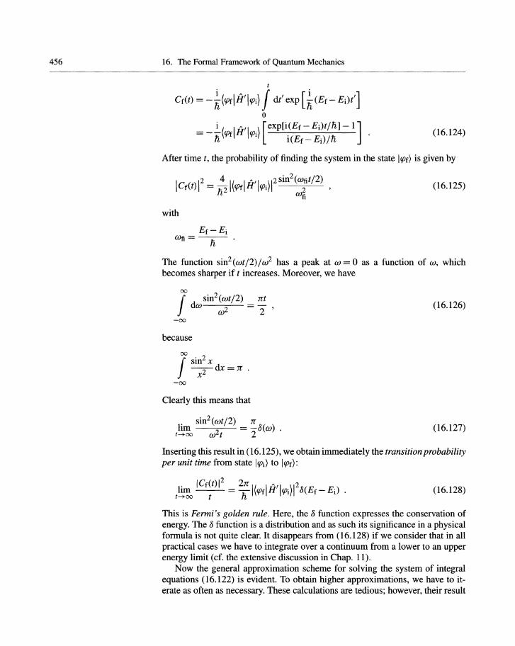
Cf(t) = -*(wIH'lfPi) f dt' exp [*(Ef- Ei)t']

o = _~( IH'I .) [eXP[i(Ef- Ei)tjftl -1]

fi fPf fPl i(Ef - Ei)/fi (16.124)

After time t, the probability of finding the system in the state Iw) is given by

(16.125)

with

The function sin2(wt/2)/u} has a peak at w = 0 as a function of w, which becomes sharper if t increases. Moreover, we have

-00

because

00

f sin2 x -2dx-Jr.

X -00

Clearly this means that

sin2(wt/2) Jr lim 2 = -8(w)

t-+oo W t 2

(16.126)

(16.127)

Inserting this result in (16.125), we obtain immediately the transition probability per unit time from state IfPi) to IfPf):

(16.128)

This is Fermi's golden rule. Here, the 8 function expresses the conservation of energy. The 8 function is a distribution and as such its significance in a physical formula is not quite clear. It disappears from (16.128) if we consider that in all practical cases we have to integrate over a continuum from a lower to an upper energy limit (cf. the extensive discussion in Chap. 11).

Now the general approximation scheme for solving the system of integral equations (16.122) is evident. To obtain higher approximations, we have to iterate as often as necessary. These calculations are tedious; however, their result


is simple enough to be presented here without proof. Generally the transition probability per time for the transition i -+ f is given by

. = -IMfil 8(Ef- Ei) ( transition probability) 21T 2

time i-+f n (16.129)

Here, the transition matrix Mfi reads:

Mfi = (fl H"Ii) + L (flH'II}(II~/li) [ Ei- EI+l11

+ LL (flH'II) (l1H'IIl) (III H' Ii) + .... [ II (Ei - E[ +il1)(Ej - Ell +il1)

(16.130)

To simplify the formula, we have abbreviated (lPflH'llPi) == (flH'li), etc. The states I, I I are intermediate states via which the higher-order transitions proceed. The infinitesimal quantity 11, which appears in the denominators, is positive and indicates how the singularities in the expression Mfi 7 are to be treated.

7 See the extensive presentation of perturbation theory in Chap. 11 and, e.g., in A.S. Davydov: Quantum Mechanics (Pergamon, Oxford 1965), Chap. VII; L.I. Schiff: Quantum Mechanics, 3rd ed. (McGraw-Hill, New York 1968), Chap. 8; A. Messiah: Quantum Mechanics, Vol. II (North-Holland, Amsterdam 1965).

457

quantum mechanics || the formal framework of quantum mechanics

Documents