quantitative finance research centre · gratefully acknowledges a visiting professor appointment at...
TRANSCRIPT
QUANTITATIVE FINANCE RESEARCH CENTRE QUANTITATIVE F
INANCE RESEARCH CENTRE
QUANTITATIVE FINANCE RESEARCH CENTRE
Research Paper 315 October 2012
An Evolutionary CAPM Under
Heterogeneous Beliefs
Carl Chiarella, Roberto Dieci, Xue-Zhong He and Kai Li
ISSN 1441-8010 www.qfrc.uts.edu.au
AN EVOLUTIONARY CAPM UNDER HETEROGENEOUS
BELIEFS
CARL CHIARELLA∗, ROBERTO DIECI∗∗, XUE-ZHONG HE∗ AND KAI LI∗
*Finance Discipline Group, UTS Business School
University of Technology, Sydney
PO Box 123, Broadway, NSW 2007, Australia
**Department of Mathematics
University of Bologna
Piazza di Porta San Donato 5, I-40126 Bologna, Italy
Current version: September 25, 2012
Acknowledgement: We would like to thank Cars Hommes for a stimulating discussion in the early
stages of this project. We are grateful to valuable comments from two anonymous referees. Dieci
gratefully acknowledges a Visiting Professor Appointment at the Quantitative Finance Research
Centre, UTS Business School, during which this work was finalised. Dieci also acknowledges sup-
port from MIUR under project PRIN 2009 “Local interactions and global dynamics in economics
and finance: models and tools” and from EU COST within Action IS1104 “The EU in the new
complex geography of economic systems: models, tools and policy evaluation”. Financial sup-
port for Chiarella and He from the Australian Research Council (ARC) under Discovery Grant
(DP110104487) is gratefully acknowledged.
Corresponding author: Xue-Zhong (Tony) He, Finance Discipline Group, UTS Business School,
University of Technology, Sydney, email: [email protected]. Ph: (61 2) 9514 7726, Fax: (61 2)
9514 7722.
1

2
Abstract. Heterogeneity and evolutionary behaviour of investors are two of
the most important characteristics of financial markets. This papers incorpo-
rates the adaptive behaviour of agents with heterogeneous beliefs and establishes
an evolutionary capital asset pricing model (ECAPM) within the mean-variance
framework. We show that the rational behaviour of agents switching to better-
performing trading strategies can cause large deviations of the market price from
the fundamental value of one asset to spill over to other assets. Also, this spill-over
effect is associated with high trading volumes and persistent volatility character-
ized by significantly decaying autocorrelations of, and positive correlation between,
price volatility and trading volume.
Key words: Evolutionary CAPM, heterogeneous beliefs, market stability, spill-over
effects, volatility, trading volume.
JEL Classification: D84, G12

AN EVOLUTIONARY CAPM UNDER HETEROGENEOUS BELIEFS 3
1. Introduction
Within the rational expectations and representative agent paradigm, the Sharpe-
Lintner-Mossin (Sharpe 1964, Lintner 1965 and Mossin 1966) Capital Asset Pricing
Model (CAPM) is the most widely used tool to value returns on risky assets. How-
ever, there is considerable empirical evidence documenting cyclical behaviour of
market characteristics, including risk premium, volatility, trading volume, price and
dividend ratio, and in particular, market betas. The conditional CAPM was devel-
oped to provide a convenient way to incorporate time-varying beta and it exhibits
empirical superiority in explaining the cross-section of returns and anomalies.1 There
exists a large literature on time-varying beta models, but most of it is motivated by
econometric estimation. It is often assumed that there are discrete changes in betas
across subsamples but constant betas within subsamples.2 It has been shown that
when betas vary over time, the standard OLS inference is misspecified and cannot be
used to assess the fit of a conditional CAPM. In addition, most of the econometric
models of time-varying beta lack any economic explanation and intuition.
Most theoretical models on conditional CAPM are based on the representative
agent economy by assuming perfect rationality and homogeneous beliefs. How-
ever, empirical evidence along with unconvincing justification of the assumption
of unbounded rationality and investor psychology, have led to the incorporation of
both heterogeneity in beliefs and bounded rationality into asset pricing and finan-
cial market modelling (see the survey papers in the edited handbook of Hens and
Schenk-Hoppe (2009) for developments in this literature). Heterogeneous beliefs
and bounded rationality have become important parts of the asset pricing literature
in recent years. Over the last two decades, there is a growing body of literature
on heterogeneous agent models (HAMs) in economics and finance. HAMs consider
1See, for example, Engle (1982), Bollerslev (1986), Bollerslev et al (1988), Dybvig and Ross
(1985), Hansen and Richard (1987), Hamilton (1989, 1990), Braun et al (1990), and Jagannathan
and Wang (1996).2See Campbell and Vuolteenaho (2004), Fama and French (2006), and Lewellen and Nagel
(2006)). We point out that Ang and Chen (2007) treat betas as endogenous variables that vary
slowly and continuously over time.
4 CHIARELLA, DIECI, HE AND LI
financial markets as a nonlinear expectation-feedback system and reflect the in-
teraction of heterogeneity, bounded rationality and adaptive behaviour of agents.
Following the seminal work of Brock and Hommes (1997, 1998), various HAMs have
been developed to show that, when agents increasingly switch to better performing
strategies, this rational behaviour of agents can lead to instability of financial mar-
kets. This framework can also explain various types of market behaviour, such as
the long-term swing of market prices from the fundamental prices, asset bubbles,
market crashes, the stylized facts and various kinds of power law behaviour observed
in financial markets.3
However, most of the HAMs analysed in the literature involve a financial market
with only one risky asset and are not in the context of the CAPM. Recently, some
attempts have been made to develop HAMs with many assets.4 Within a mean-
variance framework, Chiarella et al (2010 and 2011) study a multi-asset CAPM
through a consensus belief. In a dynamic setting, Chiarella et al (2012) demon-
strate the stochastic behavior of time-varying betas and show that there can be
inconsistency between ex-ante and ex-post estimates of asset betas when agents are
heterogeneous and boundedly rational.
The aim of this paper is to extend the HAMs with one risky asset to an evolu-
tionary CAPM within the framework of HAMs to examine the impact of adaptive
behaviour of heterogeneous agents in a market with many risky assets. This paper is
closely related to Chiarella et al (2012), but also differs from it in several respects. In
3We refer the reader to Hommes (2006), LeBaron (2006), Lux (2009), Chiarella et al (2009),
Evstigneev, Hens and Schenk-Hoppe (2009) for surveys of the recent developments in this literature.4We refer the reader to Chiarella et al (2005), Westerhoff and Dieci (2006), Chen and Huang
(2008) and Marsili, Raffaelli and Ponsot (2009) for developments in multi-asset market dynamics
in the literature of HAMs. In particular, Westerhoff (2004) considers a multi-asset model with
fundamentalists who concentrate on only one market and chartists who invest in all markets;
Dieci and Westerhoff (2010a, 2010b) explore deterministic models to study two stock markets
denominated in different currencies, which are linked via the related foreign exchange market;
Chen and Huang (2008) develop a computational multi-asset artificial stock market to examine
the relevance of risk preferences and forcasting accuracy to the survival of investors; and Marsili
et al. (2009) introduce a generic model of a multi-asset financial market to show that correlation
feedback can lead to market instability when trading volumes are high.

AN EVOLUTIONARY CAPM UNDER HETEROGENEOUS BELIEFS 5
Chiarella et al (2012), the heterogeneous beliefs are modelled at the return level and
agents do not change their strategies. A spill-over effect of market instability from
one asset to others due to behavioural change of agents is demonstrated through
numerical simulations. In this paper, the heterogeneous beliefs are modelled at the
price level and agents are allowed to change their strategies based on a fitness func-
tion similar to that used by Brock and Hommes (1997, 1998). The advantage of this
setting is that we are able to examine the stability and spill-over effects analytically.
We extend the single-period static model in Chiarella et al (2011) to a dynamic
equilibrium asset pricing model. As in Chiarella et al (2012), we incorporate two
types of investors, fundamentalists and trend followers, into the model. It is found
that the instability of one asset, characterized by large fluctuations of market prices
from the fundamental prices, can spill over to other assets when agents increas-
ingly switch to better performing strategies. The spill-over effect is also associated
with high trading volumes and persistent volatility, characterized by significantly
positive and geometrically decaying autocorrelations in volume and volatility over
long time horizons. Also the correlations between trading volume and volatility of
risky assets are positive when asset payoffs are less correlated. These implications
show that the evolutionary CAPM developed in this paper can provide insight into
market characteristics related to trading volume and volatility. Also consistent with
Chiarella et al (2012), we show that the commonly used rolling window estimates
of time-varying betas may not be consistent with the ex-ante betas implied by the
equilibrium model.
The paper is organized as follows. Section 2 sets up a dynamical equilibrium asset
pricing model in the context of the CAPM to incorporate heterogeneous beliefs and
adaptive behaviour of agents. Section 3 examines analytically the stability of the
steady state equilibrium prices of the corresponding deterministic model. In Section
4, we conduct a numerical analysis of the stochastic model to explore the spill-over
effects, together with the relation between trading volumes and volatility, and the
consistency of time-varying betas between ex-ante and rolling window estimates.
Section 5 concludes. All proofs are given in the Appendix.
6 CHIARELLA, DIECI, HE AND LI
2. The Model
We consider an economy with I agents, indexed by i = 1, · · · , I, who invest in
portfolios consisting of a riskless asset with risk free rate rf and N risky assets,
indexed by j = 1, · · · , N (with N ≥ 1). Let pt = (p1,t, · · · , pN,t)⊤ be the prices,
dt = (d1,t, · · · , dN,t)⊤ be the dividends and xt := pt + dt be the payoffs of the risky
assets in period t (from t−1 to t). Let zi,t be the risky portfolio of agent i (in terms
of the number of shares of each risky asset), then the end-of-period portfolio wealth
of agent i is given by Wi,t+1 = z⊤i,t(xt+1 −Rfpt) +RfWi,t, where Rf = 1 + rf .
2.1. Optimal Portfolio. Assume that agent i has a constant absolute risk aversion
(CARA) utility ui(x) = −e−θix, where θi is the CARA coefficient. Assuming that the
wealth of agent i is conditionally normally distributed, agent i’s optimal investment
portfolio is obtained by maximizing the certainty-equivalent utility of one-period-
ahead wealth5
Ui,t(Wi,t+1) = Ei,t(Wi,t+1)−θi2V ari,t(Wi,t+1). (2.1)
Following Chiarella et al (2011), the optimal portfolio of agent i is then given by
zi,t = θ−1i Ω−1
i,t [Ei,t(xt+1)− Rfpt], (2.2)
where Ei,t(xt+1) andΩi,t = [Covi,t(xj,t+1, xk,t+1)]N×N are respectively the conditional
expectation and variance-covariance matrix of agent i about the end-of-period pay-
offs of the risky assets, evaluated at time t.
2.2. Market Equilibrium. Assume that the I investors can be grouped into H
agent-types, indexed by h = 1, · · · , H , where the agents within the same group are
homogeneous in their beliefs as well as risk aversion. The risk aversion of agents of
type h is denoted by θh. We also denote by Ih,t the number of investors in group h and
by nh,t := Ih,t/I the market fraction of agents of type h in period t. Let Eh,t(xt+1)
and Ωh,t = [Covh,t(xj,t+1, xk,t+1)]N×N be respectively the conditional expectation
and variance-covariance matrix of type-h agents at time t. Let s = (s1, · · · , sN)⊤
be the N -dimensional vector of average risky asset supply per agent. A supply
5As is well known, the maximization of (2.1) is equivalent to maximizing the expected value of the
above-defined CARA utility of wealth, maxzi,t Ei,t(ui(Wi,t+1)), provided that Wi is conditionally
normally distributed in agent i’s beliefs.
AN EVOLUTIONARY CAPM UNDER HETEROGENEOUS BELIEFS 7
shock to the market, denoted by a vector of random processes,6 is assumed to follow
ξt+1 = ξt + σκκt+1, where κt+1 is a standard normal i.i.d. random variable with
E(κt) = 0 and Cov(κt) = I. Then the market clearing condition becomes
H∑
h=1
nh,tθ−1h Ω−1
h,t [Eh,t(xt+1)−Rfpt] = s + ξt. (2.3)
2.3. Consensus Belief. We follow the construction in Chiarella et al (2011, 2012)
to define an aggregate or consensus belief. Define the “average” risk aversion co-
efficient θa,t := (∑H
h=1 nh,tθ−1h )−1, which is a market population fraction weighted
harmonic mean of the risk aversions of different types of heterogeneous agents.
Specifically, if all agents have the same risk aversion coefficient θh = θ, then the
“average” risk aversion coefficient θa,t = θ.7 Then the aggregate beliefs at time t
about variances/covariances and expected payoffs over the time interval (t, t+1) are
specified, respectively, as
Ωa,t = θ−1a,t
( H∑
h=1
nh,tθ−1h Ω−1
h,t
)−1,
Ea,t(xt+1) = θa,tΩa,t
H∑
h=1
nh,tθ−1h Ω−1
h,tEh,t(xt+1).
(2.4)
The dividend process dt is assumed to follow a martingale process
dt+1 = dt + σζζt+1, (2.5)
where ζt+1 is a standard normal i.i.d. random variable with E(ζt) = 0 and Cov(ζt) =
I, independent of κt+1. Moreover, agents are assumed to have homogeneous and cor-
rect conditional beliefs about the dividends (the unconditional expectation of which
is assumed to be constant, E(dt) = d). Following Chiarella et al (2011, 2012), the
market equilibrium prices (2.3) can therefore be rewritten as if they were determined
by a homogeneous agent endowed with average risk aversion θa,t and the consensus
beliefs Ea,t,Ωa,t, namely
pt =1
Rf
[Ea,t(pt+1) + dt − θa,tΩa,t(s+ ξt)]. (2.6)
6σκ is not necessarily a diagonal matrix, that is, the supply noise processes of the N assets can
be correlated. The same also holds for σζ in the dividend processes (2.5).
7This is the case that we use for the numerical analysis in Section 4.
8 CHIARELLA, DIECI, HE AND LI
Note that at time t the dividends dt are realized and agents formulate their beliefs
about the next period payoff xt+1 = pt+1+dt+1, based on realized prices up to time
t− 1 and the dividends dt.
2.4. Fitness. Following the discrete choice model (discussed for instance by Brock
and Hommes (1997, 1998), the market fractions nh,t of agents of type h are deter-
mined by their fitness vh,t−1, where the subscript t−1 indicates that fitness depends
only on past observed prices and dividends. The fraction of agents using strategy
of type h is thus driven by “experience” through reinforcement learning. That is,
given the fitness vh,t−1, the fraction of agents using strategy type of h is determined
by the discrete choice model,
nh,t =eηvh,t−1
Zt
, Zt =∑
h
eηvh,t−1 , (2.7)
where η > 0 is the switching intensity of choice parameter measuring how sensitive
agents are to selecting a better preforming strategy.8 If η = 0, then agents are
insensitive to past performance and pick a strategy at random with equal probability.
In the other extreme case η → ∞, all agents choose the forecast that performed best
in the last period. An increase in the intensity of choice η can therefore represent
an increase in the degree of rationality with respect to the evolutionary selection of
strategies.
Given the utility maximization problem (2.1) of agents, we use a fitness measure
that generalizes the ‘risk-adjusted profit’ introduced in Hommes (2001) (see Hommes
and Wagener (2009) for a discussion about different choice of fitness functions and
the relation), namely we set
vh,t = πh,t − πBh,t − Ch, (2.8)
where Ch ≥ 0 measures the cost of the strategy,
πh,t := z⊤h,t−1(pt + dt − Rfpt−1)−θh2z⊤h,t−1Ωh,t−1zh,t−1 (2.9)
and
πBh,t :=
(θa,t−1
θhs
)⊤
(pt + dt − Rfpt−1)−θh2
(θa,t−1
θhs
)⊤
Ωh,t−1
(θa,t−1
θhs
). (2.10)
8In fact, η is inversely related to the variance of the noise in the observation of random utility.
AN EVOLUTIONARY CAPM UNDER HETEROGENEOUS BELIEFS 9
Note that (2.9) can be naturally interpreted as the risk-adjusted profit of type
h agent. It represents the realized profit adjusted by the subjective risk under-
taken by investor h, which is consistent with investors’ utility-maximizing portfolio
choices. Expression (2.10) can be interpreted as the (risk-adjusted) profit on portfo-
lio zBh,t−1 :=θa,t−1
θhs, which represents a ‘benchmark’ portfolio for agents of type h at
time t− 1. The portfolio zBh,t−1 is proportional to the market portfolio. The propor-
tionality coefficientθa,t−1
θhtakes into account the fact that the shares of the market
portfolio of agents are positively correlated to their risk tolerance (1/θh). In the
case that all agents have the same risk aversion (so that θa,t−1 = θh), they all take
the market portfolio. Put differently, the performance measure (2.8) views strategy
h as a successful strategy only to the extent it outperforms its market benchmark
in terms of risk-adjusted profitability. More precisely, portfolio zBh,t represents the
portfolio that agents of type h would select at time t if all agents had identical be-
liefs (whichever they are) about the first and second moment of xt+1. In this case
agents would (possibly) differ only in terms of their risk aversion and zh,t = zBh,t
for all h. According to the fitness measure vh,t := πh,t − πBh,t − Ch, their portfolios
would thus have identical performance (apart from the costs). In other words, the
selected fitness measure vh,t is not affected by mere differences in risk aversion and
accounts only of the profitability generated by the competing investment rules. Note
that, in the case of zero supply of outside shares, the market clearing equation (2.6)
leads to Ea,t(xt+1)/Rf = pt. This is the case considered in Hommes (2001) for a
single-risky-asset model. The market thus behaves as if it were ‘risk-neutral’ at the
aggregate level9 in this particular case and the performance measure reduces to the
risk-adjusted profit considered in Hommes (2001).
2.5. Fundamentalists. Now we propose a model with classical heterogeneous agent-
types and consider two types of agents, fundamentalists and trend followers, or
chartists, with h = f and h = c, respectively. Following He and Li (2007), the
fundamentalists realize the existence of non-fundamental traders, such as trend fol-
lowers to be introduced in the following discussion. The fundamentalists believe that
the stock price may be driven away from the fundamental value in the short-run,
9Of course, risk aversion does affect decisions at the agent-type level.

10 CHIARELLA, DIECI, HE AND LI
but it will eventually converge to the expected fundamental value in the long-run.
Hence the conditional mean of the fundamental traders is assumed to follow
Ef,t(pt+1) = pt−1 +α(Ef,t(p∗
t+1)− pt−1), (2.11)
where p∗t = (p∗1,t, · · · , p
∗N,t) is the vector of fundamental prices and the parameter
α = diag[α1, · · · , αN ] with αj ∈ [0, 1] represents the speed of price adjustment
of the fundamentalists toward their expected fundamental value or it reflects how
confident they are in the fundamental value. The parameter αj can be different for
different risky assets. In particular, for αj = 1, the fundamental traders are fully
confident about the fundamental value of risky asset j and adjust their expected
price in the next period instantaneously to the expected fundamental value. For
αj = 0, the fundamentalists become naive traders of asset j. We also assume that
the fundamentalists have constant beliefs about the covariance matrix of the payoffs
so that Ωf,t = Ω0 := (σjk)N×N .
2.6. Fundamental Prices. To define the fundamental price p∗t , we consider a
‘standard CAPM’ with homogeneous beliefs where all agents have correct beliefs
about the fundamental prices and are fully confident about their expected funda-
mental values (that is α = diag[1, · · · , 1]). We also assume that their average risk
aversion coefficient is constant over time, θa,t = θ, and so are their common second-
moment beliefs, Ω0.10 Correspondingly we define the fundamental price as
p∗
t =1
rf(dt − θΩ0(s+ ξt)), (2.12)
which is a martingale process under the assumptions about the exogenous dividend
and market noise processes, so that
p∗
t+1 = p∗
t + ǫt+1, ǫt+1 =1
rf(σζζt+1 − θΩ0σκκt+1) ∼ Normal i.i.d. (2.13)
In this case, it follows from Eq. (2.6) that the equilibrium price is given by pt = p∗t .
Thus we can treat the benchmark CAPM case as the ‘steady state’ of the dynamics
of the heterogeneous beliefs model.
10Without switching, the average risk aversion θ is constant and corresponds to the harmonic
mean of the risk aversion coefficients of all agents. In our simulations, we will set θ = θ∗a, the
average risk aversion coefficient at the steady state solution of the model.
AN EVOLUTIONARY CAPM UNDER HETEROGENEOUS BELIEFS 11
2.7. Trend Followers. Unlike the fundamental traders, trend followers are tech-
nical traders who believe the future price change can be predicted from various
patterns or trends generated from the historical prices. They are assumed to ex-
trapolate the latest observed price change over a long-run sample mean price and to
adjust their variance estimate accordingly. More precisely, their conditional mean
and covariance matrices are assumed to satisfy
Ec,t(pt+1) = pt−1 + γ(pt−1 − ut−1), Ωc,t = Ω0 + λVt−1, (2.14)
where ut−1 and Vt−1 are sample means and covariance matrices of past market
prices pt−1,pt−2, · · · , the constant vector γ = diag[γ1, · · · , γN ] > 0 reflects the trend
following strategy, and γj measures the extrapolation rate and high (low) values of
γj correspond to strong (weak) extrapolation by trend followers, and λ measures the
sensitivity of the second-moment estimate to the sample variance. This specification
of the trend followers captures the extrapolative behavior of the trend followers, who
expect price changes to occur in the same direction as the price trend observed over
a past time window. Assume that ut−1 and Vt−1 are computed recursively as
ut−1 = δut−2 + (1− δ)pt−1,
Vt−1 = δVt−2 + δ(1− δ)(pt−1 − ut−2)(pt−1 − ut−2)⊤. (2.15)
Effectively, the sample mean and variance-covariance matrix are calculated based
on the all historical prices pt−1,pt−2, · · · , spreading back to −∞ with geometric
decaying probability weights (1 − δ)1, δ, δ2, · · · . Therefore, as δ decreases, the
weights on the latest prices increase but decay geometrically at a common rate of δ.
For γ > 0 and large δ, momentum traders calculate the trend based on a long time
horizon. In particular, when δ = 0, Ec,t(pt+1) = pt−1 and Vt−1 = 0, implying naive
behaviour by the trend followers. However, when δ = 1, ut−1 = u0 and Vt−1 = V0,
and therefore Ec,t(pt+1) = pt−1+γ(pt−1−u0), so that trend followers are momentum
traders.
2.8. The Complete Dynamic Model. Based on the analysis above, the optimal
demands of the fundamentalists and trend followers are given, respectively, by
zf,t = θ−1f Ω−1
o [pt−1 + dt +α(p∗
t − pt−1)− Rfpt] (2.16)
12 CHIARELLA, DIECI, HE AND LI
and
zc,t = θ−1c [Ω0 + λVt−1]
−1[pt−1 + dt + γ(pt−1 − ut−1)− Rfpt]. (2.17)
Finally, the general dynamic model (2.6) reduces to the random nonlinear dynamical
system
pt =θa,tRf
Ωa,t
[nf,t
θfΩ−1
0
(pt−1 +α(p∗
t − pt−1))
+nc,t
θc(Ω0 + λVt−1)
−1(pt−1 + γ(pt−1 − ut−1)
)− s− ξt
]+
1
Rf
dt,
p∗
t =1
rf(dt − θ∗aΩ0(s + ξt)),
ut = δut−1 + (1− δ)pt,
Vt = δVt−1 + δ(1− δ)(pt − ut−1)(pt − ut−1)⊤,
nf,t =1
1 + e−ηv∆,t−1,
ξt = ξt−1 + σκκt,
dt = dt−1 + σζζt,
(2.18)
where
θa,t =(nf,t
θf+
nc,t
θc
)−1
, Ωa,t =1
θa,t
(nf,t
θfΩ−1
0 +nc,t
θc(Ω0 + λVt−1)
−1)−1
,
v∆,t := vf,t − vc,t =
(zf,t−1 −
θa,t−1s
θf
)⊤(pt + dt −Rfpt−1 −
θf2Ω0(zf,t−1 +
θa,t−1s
θf)
)
−
(zc,t−1 −
θa,t−1s
θc
)⊤(pt + dt −Rfpt−1 −
θc2(Ω0 + λVt−2)(zc,t−1 +
θa,t−1s
θc)
)− C∆,
nc,t = 1− nf,t, C∆ = Cf − Cc ≥ 0.
In summary, we have established an adaptively heterogeneous beliefs model of
asset prices under the CAPM framework. The resulting model is characterized by
a stochastic difference system with seven variables, which is difficult to analyze
directly. To understand the interaction of the deterministic dynamics and noise
processes, we first study the dynamics of the corresponding deterministic model in
Section 3. The stochastic model (2.18) is then analyzed in Section 4.
AN EVOLUTIONARY CAPM UNDER HETEROGENEOUS BELIEFS 13
3. Dynamics of the Deterministic Model
By assuming that the fundamental price and the dividend are constants p∗t =
p∗, dt = d, and there is no supply shock ξt = 0, the system (2.18) becomes the
deterministic dynamical system11
pt =θa,tRf
Ωa,t
[nf,t
θfΩ−1
0
(pt−1 +α(p∗ − pt−1)
)
+nc,t
θc(Ω0 + λVt−1)
−1(pt−1 + γ(pt−1 − ut−1)
)− s
]+
1
Rf
d,
ut = δut−1 + (1− δ)pt,
Vt = δVt−1 + δ(1− δ)(pt − ut−1)(pt − ut−1)⊤,
nf,t =1
1 + e−ηv∆,t−1.
(3.1)
The dynamical system (3.1) should not be interpreted as a deterministic approx-
imation of stochastic system (2.18), based on some type of asymptotic convergence,
but just as a system obtained by setting the dividend, the supply and the funda-
mental price at their unconditional mean levels. The analysis of this ‘deterministic
skeleton’ is a common practice in the heterogeneous-agent literature, and it is aimed
at gaining some initial insights into the impact of the parameters on the underlying
dynamics. Although the properties of the deterministic skeleton do not carry over
to the stochastic model in general, important connections between the dynamical
structure of the stochastic model and that of the underlying deterministic model ex-
ist and have been highlighted in recent literature on stochastic heterogeneous-agent
models (see, e.g. Chiarella, He and Zheng (2011) and Zhu, Wang and Guo (2011)).
The system (3.1) has a unique steady state (pt,ut,Vt, nf,t) = (p∗,p∗, 0, n∗f),
where, following Eq. (2.12), the fundamental steady state price, p∗, is given by
p∗ =1
rf(d− θ∗aΩ0s) (3.2)
11The state variables pt, ut, Vt and nf,t in Eq. (3.1) can be expressed in terms of pt−1, ut−1,
Vt−1, nf,t−1, pt−2, ut−2, Vt−2 and nf,t−2, which have N , N , N(N + 1)/2, 1, N , N , N(N + 1)/2
and 1 dimensions respectively. So the dimension of the system (3.1) is N2 +5N + 2. For instance,
when N = 1, it is an 8-dimensional system.
14 CHIARELLA, DIECI, HE AND LI
and n∗f = 1/(1 + eηC∆). Hence, at the steady state, n∗
c = 1 − n∗f and θa,t = θ∗a =
1/(n∗f/θf + n∗
c/θc). Let θ0 := θf/θc. Note that if θf = θc = θ, then θa,t = θ and
θ0 = 1.
For the N2+5N +2 dimensional system (3.1), we are able to obtain the following
proposition on the local stability of the steady state. The proof is given in the
appendix.
Proposition 3.1. For the system (3.1),
(i) if Rf ≥ δ(1 + γj) for all j ∈ 1, · · · , N, then the steady state (p∗,p∗,0, n∗f)
is locally asymptotically stable;
(ii) if Rf < δ(1 + γj) for all j ∈ 1, · · · , N, then the steady state is locally
asymptotically stable when C∆ 6= 0 and η < ηj := 1C∆
lnRf−δ(1−αj )
θ0[δ(1+γj )−Rf ]for
all j ∈ 1, · · · , N and undergoes a Hopf bifurcation when η = ηj for some
j ∈ 1, · · · , N. If C∆ = 0, then the steady state is locally asymptotically
stable when θ0γj < αj + (1 + θ0)(Rf
δ− 1) for all j;
(iii) if Rf < δ(1 + γj) for some j ∈ Jo ⊆ 1, · · · , N, then the steady state is
locally asymptotically stable when η < ηm := minj∈Jo ηj and undergoes a Hopf
bifurcation when η = ηm.
The results in Proposition 3.1 are significant with respect to the intuitive and
simple conditions on the stability of the steady state for such a high dimensional
system. First, when the trend followers are not very active (so that γj ≤ Rf/δ− 1),
the steady state of the system is stable. Second, the stability condition (ii) is
equivalent to
Rf
δ− 1 < γj <
(Rf
δ− 1)(1 + θ0e
ηC∆) + αj
θ0eηC∆, j = 1, · · · , N.
Hence, even when the trend followers are active (so that γj > Rf/δ−1), the system
can still be stable when the fundamentalists dominate the market at the steady state
or, equivalently, the switching intensity is sufficiently small. In short, Proposition
3.1 shows clearly that increases in Cc, αj and θc stabilize the system, while increases
in Cf , δ, γ and θf destabilize the system. Intuitively, the fundamentalists play a
stabilizing role in the market. The activity of fundamentalists is enhanced with
AN EVOLUTIONARY CAPM UNDER HETEROGENEOUS BELIEFS 15
an increase in αj or decreases in Cf (since a decrease in Cf increases the market
fraction of fundamentalists) and θf (since a decrease in θf increases fundamentalists’
long/short position when the fundamental price moves away from the market price).
To understand how the impact of switching in a market with many risky assets
is different from a market with a single risky asset, we consider a special case where
agents invest in a market with one risk-free asset and one risky asset, say asset j.
In this case, system (3.1) reduces to
pj,t =djRf
+1
Rf
(nf,t
θfσ2j
+ nc,t
θc(σ2j+λVj,t−1)
)[nf,t
(pj,t−1 + αj(p
∗j − pj,t−1)
)
θfσ2j
+nc,t
(pj,t−1 + γj(pj,t−1 − uj,t−1)
)
θc(σ2j + λVj,t−1)
− sj
],
uj,t = δuj,t−1 + (1− δ)pj,t,
Vj,t = δVj.t−1 + δ(1− δ)(pj,t − uj,t−1)2,
nf,t =1
1 + e−ηv∆,t−1.
(3.3)
The dynamics of the system (3.3) can be characterized by the following proposition
(the proof is given in the appendix).
Proposition 3.2. For the system (3.3),
(i) if Rf ≥ δ(1 + γj), then the steady state (p∗j , p∗j , 0, n
∗f) of the system is always
locally asymptotically stable;
(ii) if Rf < δ(1 + γj), then the steady state is locally asymptotically stable when
η < ηj and C∆ 6= 0 and undergoes a Hopf bifurcation when η = ηj. When
C∆ = 0, the steady state is locally asymptotically stable if θ0γj < αj + (1 +
θ0)(Rf
δ− 1).
By comparing the local stability conditions in Propositions 3.1 and 3.2, one can
see that the stability conditions of each risky asset due to the increasing switching
intensity are independent of the parameters specific to any other asset and, sur-
prisingly, the correlations among risky assets have no impact on the local stability
16 CHIARELLA, DIECI, HE AND LI
properties.12 This result is due to the peculiar properties of the Jacobian matrix
and the adaptive behaviour considered (this becomes clear from the proofs in the
appendix). Hence the local stability properties of asset j in the multi-asset model
are exactly the same as if asset j was considered in isolation (that is, in the model
with only risky asset j and the risk-free asset).
Propositions 3.1 and 3.2 provide an initial insight into the mechanisms governing
the joint price dynamics of multiple risky assets, showing that locally instability
plays a very small role in the spill-over phenomena that we will discuss in what
follows, but globally the instability of one asset can spill over to the other assets due
to its correlations with other assets.
To better understand the implications of Propositions 3.1 and 3.2 and the price
dynamics of the model, we consider an example of two risky assets and a riskless
asset with
Ω0 =
σ2
1 ρ12σ1σ2
ρ12σ1σ2 σ22
and set13 s = (0.1, 0.1)⊤, θf = 1, θc = 1, λ = 1.5, Cf = 4, Cc = 1, ρ12 = 0.5,
δ = 0.98, γ = diag[0.3, 0.3] and α = diag[0.4, 0.5]. We choose the annual values14
of the following parameters: rf = 0.025, σ1 = 0.6, σ2 = 0.4 and d = (0.08, 0.05)⊤.
In this paper, we consider monthly time steps (i.e. K = 12).
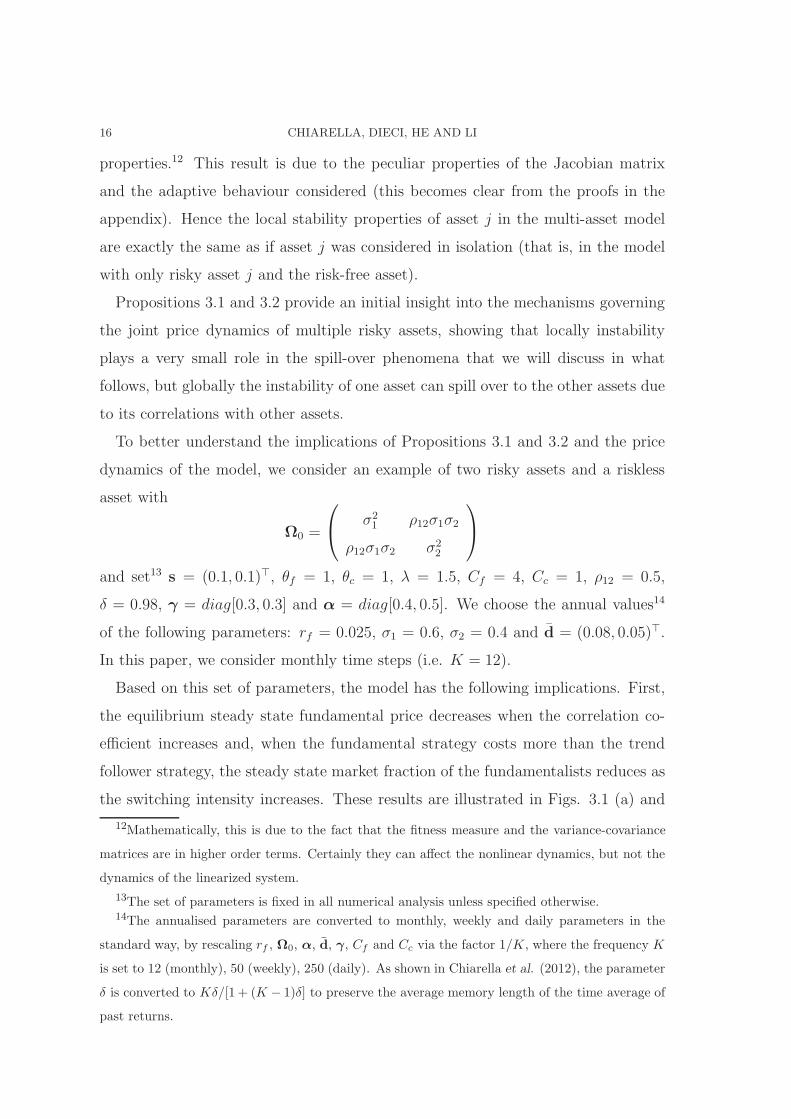
Based on this set of parameters, the model has the following implications. First,
the equilibrium steady state fundamental price decreases when the correlation co-
efficient increases and, when the fundamental strategy costs more than the trend
follower strategy, the steady state market fraction of the fundamentalists reduces as
the switching intensity increases. These results are illustrated in Figs. 3.1 (a) and
12Mathematically, this is due to the fact that the fitness measure and the variance-covariance
matrices are in higher order terms. Certainly they can affect the nonlinear dynamics, but not the
dynamics of the linearized system.
13The set of parameters is fixed in all numerical analysis unless specified otherwise.14The annualised parameters are converted to monthly, weekly and daily parameters in the
standard way, by rescaling rf , Ω0, α, d, γ, Cf and Cc via the factor 1/K, where the frequency K
is set to 12 (monthly), 50 (weekly), 250 (daily). As shown in Chiarella et al. (2012), the parameter
δ is converted to Kδ/[1 + (K − 1)δ] to preserve the average memory length of the time average of
past returns.
AN EVOLUTIONARY CAPM UNDER HETEROGENEOUS BELIEFS 17
−1 −0.5 0 0.5 10
0.5
1
1.5
2
2.5
3
ρ12
p*
p1*
p2*
(a) Steady-state prices
0 2 4 6 8 100.05
0.1
0.15
0.2
0.25
0.3
0.35
0.4
0.45
0.5
η
n*f
(b) Steady-state market fraction
Figure 3.1. (a) The fundamental steady state price p∗ = (p∗1, p∗2)
as a function of the correlation ρ12 with η = 1; (b) The equilibrium
market fractions of fundamentalists n∗f as a function of the switching
intensity η.
(b) respectively for the two-asset system (3.1). In fact, Eq. (3.2) determines the
dependence of the steady state fundamental price on the parameters. Fig. 3.1 (a)
illustrates a negative linear relationship between the fundamental steady state price
p∗ = (p∗1, p∗2) and the correlation ρ12.
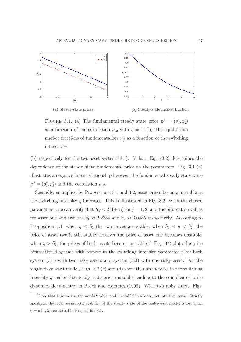
Secondly, as implied by Propositions 3.1 and 3.2, asset prices become unstable as
the switching intensity η increases. This is illustrated in Fig. 3.2. With the chosen
parameters, one can verify that Rf < δ(1+γj) for j = 1, 2, and the bifurcation values
for asset one and two are η1 ≈ 2.2384 and η2 ≈ 3.0485 respectively. According to
Proposition 3.1, when η < η1 the two prices are stable; when η1 < η < η2, the
price of asset two is still stable, however the price of asset one becomes unstable;
when η > η2, the prices of both assets become unstable.15 Fig. 3.2 plots the price
bifurcation diagrams with respect to the switching intensity parameter η for both
system (3.1) with two risky assets and system (3.3) with one risky asset. For the
single risky asset model, Figs. 3.2 (c) and (d) show that an increase in the switching
intensity η makes the steady state price unstable, leading to the complicated price
dynamics documented in Brock and Hommes (1998). With two risky assets, Figs.
15Note that here we use the words ‘stable’ and ‘unstable’ in a loose, yet intuitive, sense. Strictly
speaking, the local asymptotic stability of the steady state of the multi-asset model is lost when
η = minj ηj , as stated in Proposition 3.1.
18 CHIARELLA, DIECI, HE AND LI
0 0.5 1 1.5 2 2.5 3 3.5 40.9
0.95
1
1.05
1.1
1.15
1.2
1.25
1.3
1.35
1.4
η
p1
(a) Asset one price in the two-asset model
0 0.5 1 1.5 2 2.5 3 3.5 40.76
0.78
0.8
0.82
0.84
0.86
0.88
0.9
0.92
0.94
η
p2
(b) Asset two price in the two-asset model
0 0.5 1 1.5 2 2.5 3 3.5 4
1.5
1.55
1.6
1.65
1.7
1.75
1.8
1.85
1.9
η
p1
(c) Price in a single asset one model
0 0.5 1 1.5 2 2.5 3 3.5 41.26
1.28
1.3
1.32
1.34
1.36
1.38
1.4
1.42
1.44
η
p2
(d) Price in a single asset two model
Figure 3.2. The bifurcations of the two risky asset prices with re-
spect to η (a) and (b), the two asset model (3.1); and (c) and (d) the
single risky asset model (3.3).
3.2 (a) and (b) show that the steady state is stable when the switching intensity η
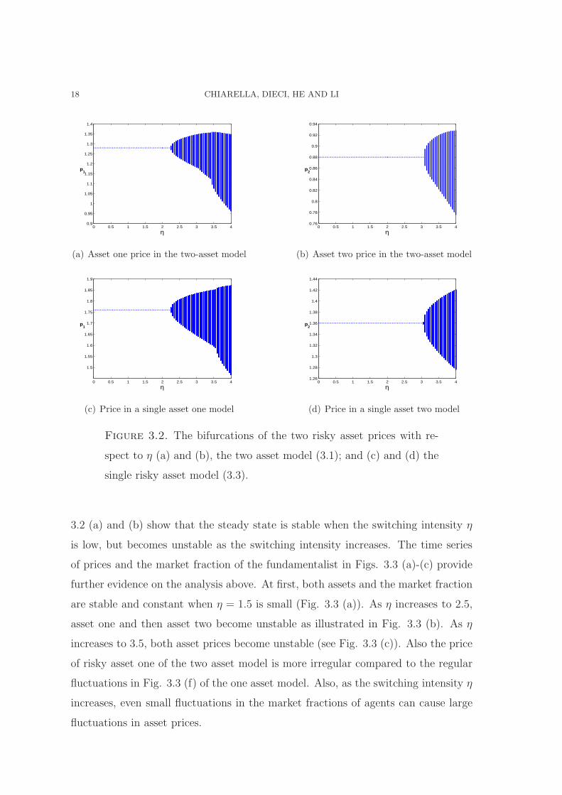
is low, but becomes unstable as the switching intensity increases. The time series
of prices and the market fraction of the fundamentalist in Figs. 3.3 (a)-(c) provide
further evidence on the analysis above. At first, both assets and the market fraction
are stable and constant when η = 1.5 is small (Fig. 3.3 (a)). As η increases to 2.5,
asset one and then asset two become unstable as illustrated in Fig. 3.3 (b). As η
increases to 3.5, both asset prices become unstable (see Fig. 3.3 (c)). Also the price
of risky asset one of the two asset model is more irregular compared to the regular
fluctuations in Fig. 3.3 (f) of the one asset model. Also, as the switching intensity η
increases, even small fluctuations in the market fractions of agents can cause large
fluctuations in asset prices.
AN EVOLUTIONARY CAPM UNDER HETEROGENEOUS BELIEFS 19
0 1000 2000 3000 4000 50000.8
0.9
1
1.1
1.2
1.3
P
t
0 1000 2000 3000 4000 5000−1
−0.5
0
0.5
1
1.5
nf
p1
p2
nf
(a)
0 1000 2000 3000 4000 50000.8
1
1.2
1.4
P
t
0 1000 2000 3000 4000 50000.3486
0.3486
0.3486
0.3487
nf
p1
p2
nf
(b)
0 1000 2000 3000 4000 50000.5
1
1.5
P
t
0 1000 2000 3000 4000 50000.2935
0.294
0.2945
nf
p1
p2
nf
(c)
0 1000 2000 3000 4000 50000.5
1
1.5
2
2.5
3
P
t
0 1000 2000 3000 4000 5000−1
−0.5
0
0.5
1
1.5
nf
p1
nf
(d)
0 1000 2000 3000 4000 50001.7
1.75
1.8
1.85
P
t
0 1000 2000 3000 4000 50000.3486
0.3486
0.3486
0.3487
nf
p1
nf
(e)
0 1000 2000 3000 4000 50001.4
1.6
1.8
2
P
t
0 1000 2000 3000 4000 50000.2938
0.294
0.2942
0.2944
nf
p1
nf
(f)
Figure 3.3. Time series plots of p1,t, p2,t and nf,t in the two-asset
model ((a)-(c)) and of p1,t in the single-asset one model ((d)-(f)) with
η = 1.5 in (a) and (d); η = 2.5 in (b) and (e); and η = 3.5 in (c) and
(f).
Thirdly, the model displays a very interesting spill-over effect, which can be very
different from portfolio effect. As we discussed earlier, the stability is a local result
and the stability conditions of the risky assets are independent among the risky
assets. When one asset becomes unstable, one would expect the spill-over of insta-
bility of the asset to spread to the other assets due to the portfolio effect. However,
this may not always be the case, as demonstrated in Fig. 3.4. For η = 2.5, Fig.
3.4 (a) shows that the price is unstable for asset one, but stable for asset two. In-
tuitively, the price fluctuations in asset one would be caused by changing portfolio
positions taken by the two types of agents for asset one, which is confirmed by Fig.
3.4 (c). However, this intuition does not carry over to asset two for which the price
is constant but the portfolio positions taken by agents for the asset are also varying,
20 CHIARELLA, DIECI, HE AND LI
0 1000 2000 3000 4000 50000.8
1
1.2
1.4
P
t
0 1000 2000 3000 4000 50000.3486
0.3486
0.3486
0.3487
nf
p1
p2
nf
(a) Prices
0 1000 2000 3000 4000 50000.17
0.18
0.19
0.2
0.21
0.22
0.23
0.24
0.25
0.26
t
Val
ues
of th
e R
isky
Por
tfolio
s
FundamentalistsTrend Followers
(b) Values of the risky portfolios
0 1000 2000 3000 4000 50000.02
0.04
0.06
0.08
0.1
0.12
0.14
0.16
0.18
0.2
t
Pos
ition
s in
Ass
et O
ne
FundamentalistsTrend Followers
(c) Positions in Asset One
0 1000 2000 3000 4000 50000.02
0.04
0.06
0.08
0.1
0.12
0.14
0.16
t
Pos
ition
s in
Ass
et T
wo
FundamentalistsTrend Followers
(d) Positions in Asset Two
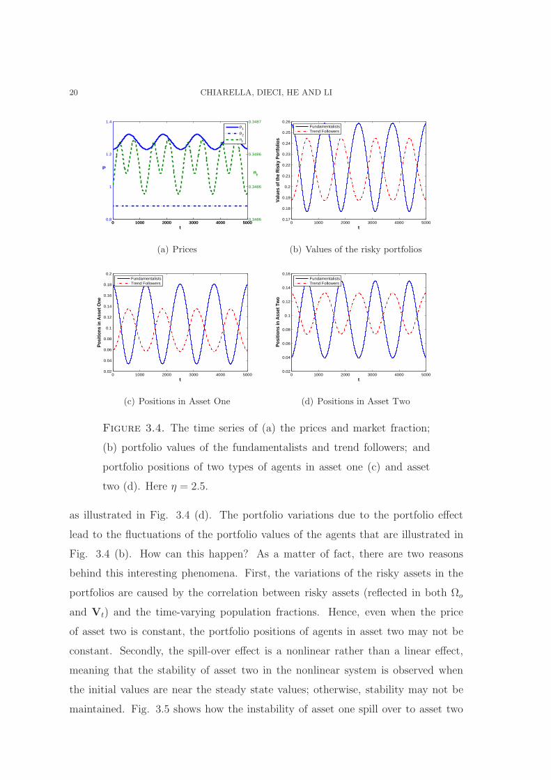
Figure 3.4. The time series of (a) the prices and market fraction;
(b) portfolio values of the fundamentalists and trend followers; and
portfolio positions of two types of agents in asset one (c) and asset
two (d). Here η = 2.5.
as illustrated in Fig. 3.4 (d). The portfolio variations due to the portfolio effect
lead to the fluctuations of the portfolio values of the agents that are illustrated in
Fig. 3.4 (b). How can this happen? As a matter of fact, there are two reasons
behind this interesting phenomena. First, the variations of the risky assets in the
portfolios are caused by the correlation between risky assets (reflected in both Ωo
and Vt) and the time-varying population fractions. Hence, even when the price
of asset two is constant, the portfolio positions of agents in asset two may not be
constant. Secondly, the spill-over effect is a nonlinear rather than a linear effect,
meaning that the stability of asset two in the nonlinear system is observed when
the initial values are near the steady state values; otherwise, stability may not be
maintained. Fig. 3.5 shows how the instability of asset one spill over to asset two
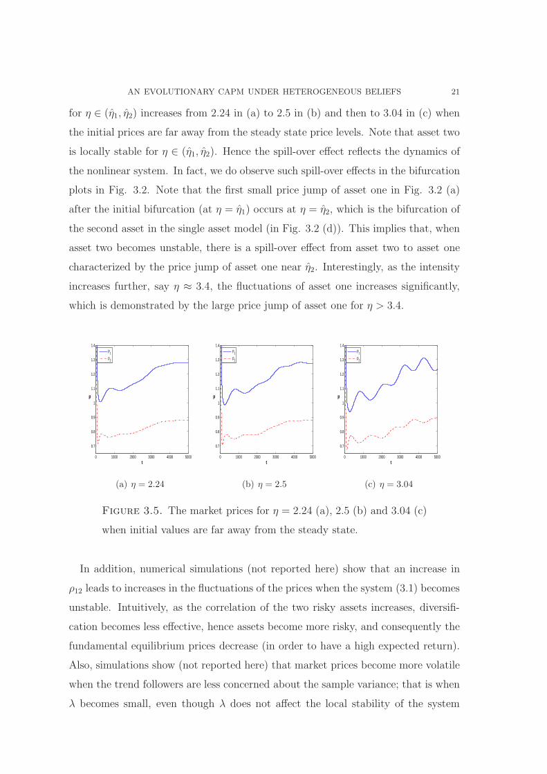
AN EVOLUTIONARY CAPM UNDER HETEROGENEOUS BELIEFS 21
for η ∈ (η1, η2) increases from 2.24 in (a) to 2.5 in (b) and then to 3.04 in (c) when
the initial prices are far away from the steady state price levels. Note that asset two
is locally stable for η ∈ (η1, η2). Hence the spill-over effect reflects the dynamics of
the nonlinear system. In fact, we do observe such spill-over effects in the bifurcation
plots in Fig. 3.2. Note that the first small price jump of asset one in Fig. 3.2 (a)
after the initial bifurcation (at η = η1) occurs at η = η2, which is the bifurcation of
the second asset in the single asset model (in Fig. 3.2 (d)). This implies that, when
asset two becomes unstable, there is a spill-over effect from asset two to asset one
characterized by the price jump of asset one near η2. Interestingly, as the intensity
increases further, say η ≈ 3.4, the fluctuations of asset one increases significantly,
which is demonstrated by the large price jump of asset one for η > 3.4.
0 1000 2000 3000 4000 5000
0.7
0.8
0.9
1
1.1
1.2
1.3
1.4
t
p
p
1
p2
(a) η = 2.24
0 1000 2000 3000 4000 5000
0.7
0.8
0.9
1
1.1
1.2
1.3
1.4
t
p
p
1
p2
(b) η = 2.5
0 1000 2000 3000 4000 5000
0.7
0.8
0.9
1
1.1
1.2
1.3
1.4
t
p
p
1
p2
(c) η = 3.04
Figure 3.5. The market prices for η = 2.24 (a), 2.5 (b) and 3.04 (c)
when initial values are far away from the steady state.
In addition, numerical simulations (not reported here) show that an increase in
ρ12 leads to increases in the fluctuations of the prices when the system (3.1) becomes
unstable. Intuitively, as the correlation of the two risky assets increases, diversifi-
cation becomes less effective, hence assets become more risky, and consequently the
fundamental equilibrium prices decrease (in order to have a high expected return).
Also, simulations show (not reported here) that market prices become more volatile
when the trend followers are less concerned about the sample variance; that is when
λ becomes small, even though λ does not affect the local stability of the system
22 CHIARELLA, DIECI, HE AND LI
(3.1). In fact, when λ becomes small, the demand of the trend followers increases
so that they become more active in the market, leading to a more volatile market.
In summary, we have shown that the rational behaviour of agents in switching
to better performing strategies can lead to market instability and a non-linear spill-
over of price fluctuations from one asset to other assets. The nonlinear dynamics
due to the spill-over effect can lead to high trading volume and high volatility. This
becomes clearer in the discussion of the stochastic model in the next section.
4. Price Behaviour of the Stochastic Model
In this section, through numerical simulations, we first focus on the spill-over effect
by examining the interaction between the dynamics of the deterministic model and
the noise processes and explore the potential power of the model to explain price
deviations from the fundamental prices and also high volatility. We then provide an
evolutionary capital asset pricing model (ECAPM) and compare the ex-ante betas
with the rolling window estimates of the betas used in the literature. Finally we
study the relationship between the price volatility and trading volumes. We choose
σκ = diag[0.001, 0.001] and σζ = diag[0.002, 0.002], representing 0.1% and 0.2%
standard deviations of the noisy supply and dividend processes respectively in this
section.
4.1. The Spill-over Effect. First, we examine the spill-over effect by exploring the
joint impact of the switching intensity η and the two noise processes on the market
price dynamics. To examine the impact of stability of the deterministic model on
the price dynamics, in particular, the time-varying betas, for the stochastic model,
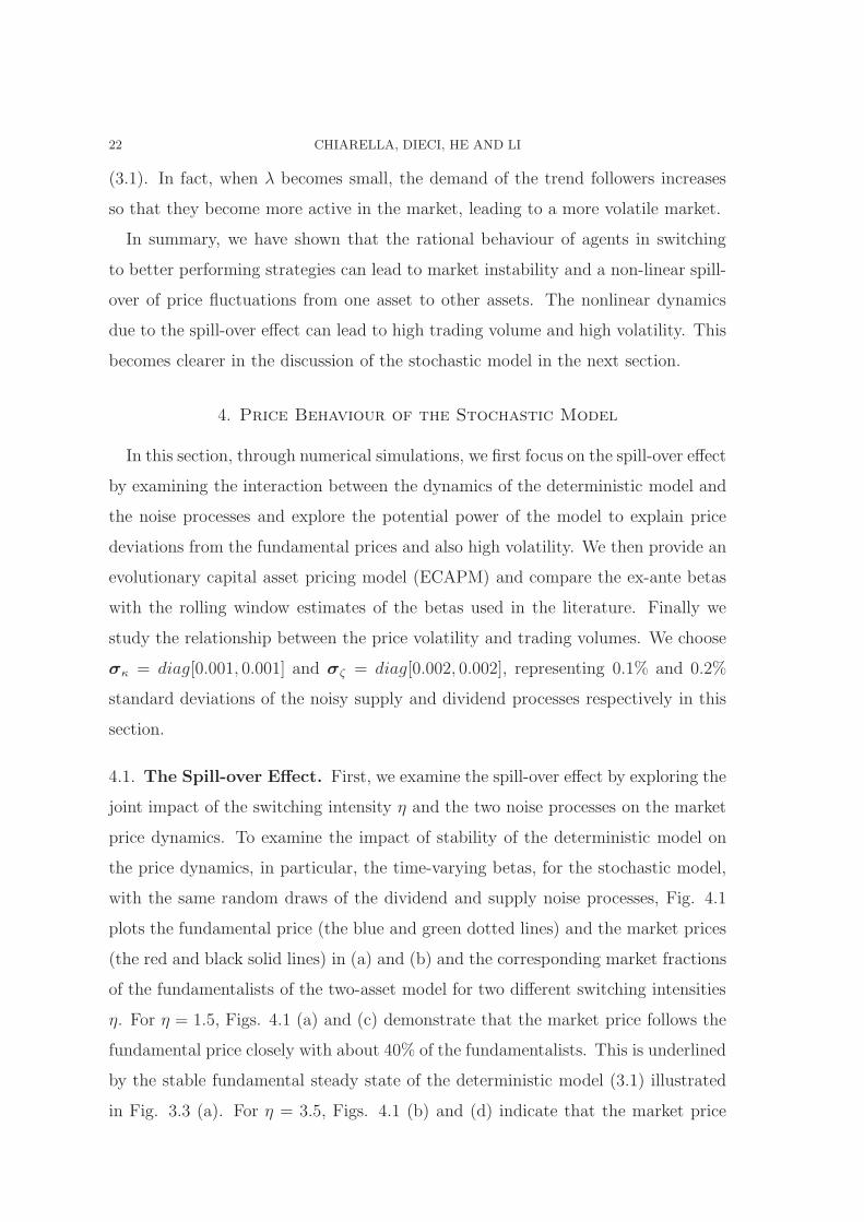
with the same random draws of the dividend and supply noise processes, Fig. 4.1
plots the fundamental price (the blue and green dotted lines) and the market prices
(the red and black solid lines) in (a) and (b) and the corresponding market fractions
of the fundamentalists of the two-asset model for two different switching intensities
η. For η = 1.5, Figs. 4.1 (a) and (c) demonstrate that the market price follows the
fundamental price closely with about 40% of the fundamentalists. This is underlined
by the stable fundamental steady state of the deterministic model (3.1) illustrated
in Fig. 3.3 (a). For η = 3.5, Figs. 4.1 (b) and (d) indicate that the market price
AN EVOLUTIONARY CAPM UNDER HETEROGENEOUS BELIEFS 23
0 1000 2000 3000 4000 50000.5
1
1.5
2
2.5
3
t
p
1
p*1
p2
p*2
(a) Prices with η = 1.5
0 1000 2000 3000 4000 50000.5
1
1.5
2
2.5
3
t
p
1
p*1
p2
p*2
(b) Prices with η = 3.5
0 1000 2000 3000 4000 50000.406
0.4062
0.4064
0.4066
0.4068
0.407
0.4072
0.4074
0.4076
0.4078
0.408
t
nf
(c) Market fraction with η = 1.5
0 1000 2000 3000 4000 50000.2905
0.291
0.2915
0.292
0.2925
0.293
0.2935
0.294
0.2945
0.295
0.2955
t
nf
(d) Market fraction with η = 3.5
Figure 4.1. The time series of the fundamental price (the dotted
line) and the market prices (the solid line) of the two-asset model
with (a) η = 1.5 and (b) η = 3.5, and the corresponding market
fractions of the fundamentalists in (c) and (d).
fluctuates around the fundamental price in a cyclical fashion with about 29% of the
fundamentalists, which is underlined by the bifurcation of periodic oscillations of
the corresponding deterministic model (see Fig. 3.3 (c)). Corresponding to Fig. 3.4
for the deterministic model, Fig. 4.2 plots the time series of the prices in (a), the
market fraction of the fundamentalists in (b), the portfolio values of the two agents
in (c), the portfolio positions in asset one (d) and asset two (e) of the stochastic
model. The large fluctuations of the stochastic model, in particular in the portfolio
values and the portfolio positions, compared to the deterministic model reflect the
impact of the nonlinear interaction of the spill-over effects and the noise processes.
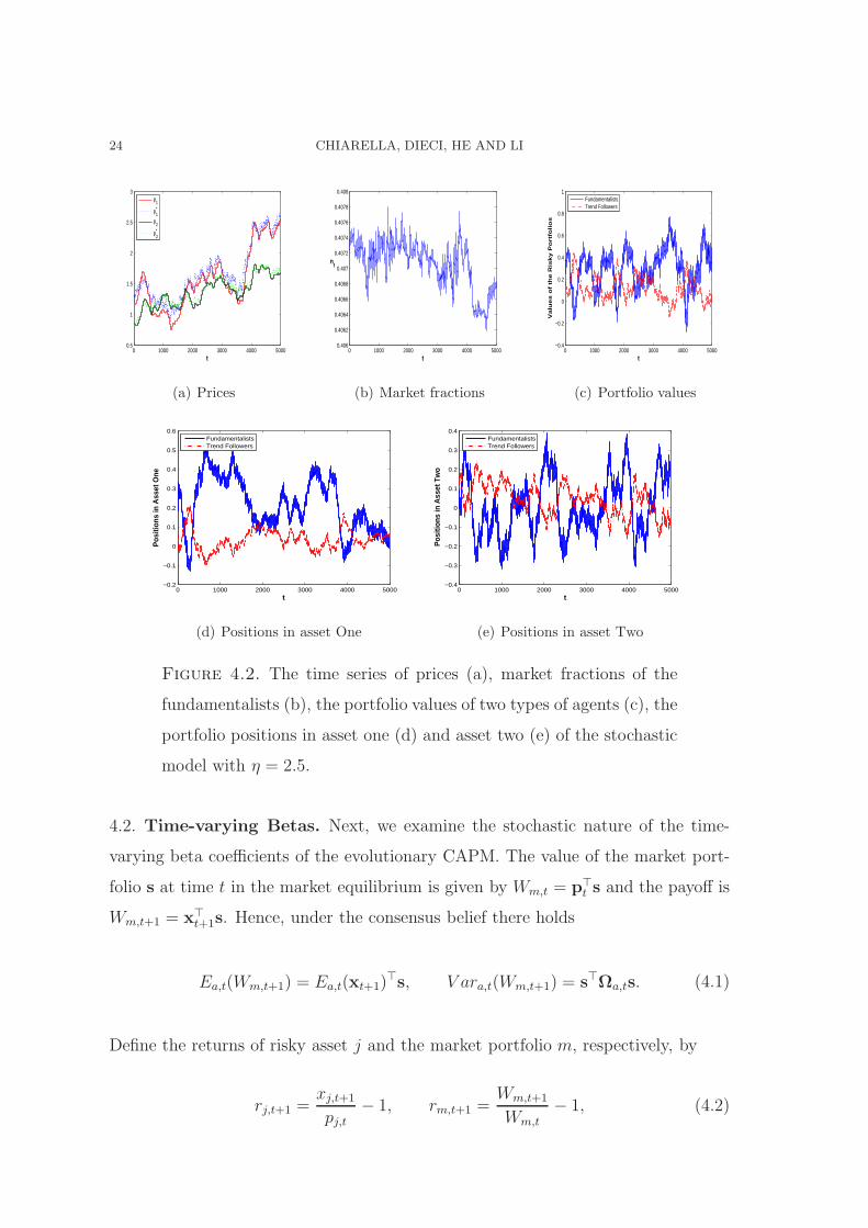
24 CHIARELLA, DIECI, HE AND LI
0 1000 2000 3000 4000 50000.5
1
1.5
2
2.5
3
t
p
1
p*1
p2
p*2
(a) Prices
0 1000 2000 3000 4000 50000.406
0.4062
0.4064
0.4066
0.4068
0.407
0.4072
0.4074
0.4076
0.4078
0.408
t
nf
(b) Market fractions
0 1000 2000 3000 4000 5000−0.4
−0.2
0
0.2
0.4
0.6
0.8
1
t
Va
lue
s o
f th
e R
isky P
ort
folio
s
FundamentalistsTrend Followers
(c) Portfolio values
0 1000 2000 3000 4000 5000−0.2
−0.1
0
0.1
0.2
0.3
0.4
0.5
0.6
t
Pos
ition
s in
Ass
et O
ne
FundamentalistsTrend Followers
(d) Positions in asset One
0 1000 2000 3000 4000 5000−0.4
−0.3
−0.2
−0.1
0
0.1
0.2
0.3
0.4
t
Pos
ition
s in
Ass
et T
wo
FundamentalistsTrend Followers
(e) Positions in asset Two
Figure 4.2. The time series of prices (a), market fractions of the
fundamentalists (b), the portfolio values of two types of agents (c), the
portfolio positions in asset one (d) and asset two (e) of the stochastic
model with η = 2.5.
4.2. Time-varying Betas. Next, we examine the stochastic nature of the time-
varying beta coefficients of the evolutionary CAPM. The value of the market port-
folio s at time t in the market equilibrium is given by Wm,t = p⊤t s and the payoff is
Wm,t+1 = x⊤t+1s. Hence, under the consensus belief there holds
Ea,t(Wm,t+1) = Ea,t(xt+1)⊤s, V ara,t(Wm,t+1) = s⊤Ωa,ts. (4.1)
Define the returns of risky asset j and the market portfolio m, respectively, by
rj,t+1 =xj,t+1
pj,t− 1, rm,t+1 =
Wm,t+1
Wm,t
− 1, (4.2)
AN EVOLUTIONARY CAPM UNDER HETEROGENEOUS BELIEFS 25
0 200 400 600 800 10000.4
0.6
0.8
1
1.2
1.4
1.6
1.8
2
t
pt
p
1,t
p2,t
(a) Prices
0 200 400 600 800 10000
0.002
0.004
0.006
0.008
0.01
0.012
0.014
t
rt
rm,t
r1,t
r2,t
(b) Returns
0 200 400 600 800 1000
0.35
0.4
0.45
0.5
0.55
0.6
0.65
0.7
t
ω
1,t
ω2,t
(c) Market portfolio
0 200 400 600 800 10000
0.2
0.4
0.6
0.8
1
1.2
1.4
1.6
1.8
2
t
Ex−
an
te B
eta
s
asset 1asset 2
(d) Ex-ante betas
0 200 400 600 800 10000
0.5
1
1.5
2
2.5
t
Re
aliz
ed
Be
tas
asset 1asset 2
(e) Rolling estimates of betas
with rolling window of 100
0 200 400 600 800 10000.2
0.4
0.6
0.8
1
1.2
1.4
1.6
1.8
2
t
Re
aliz
ed
Be
tas
asset 1asset 2
(f) Rolling estimates of betas
with rolling window of 300
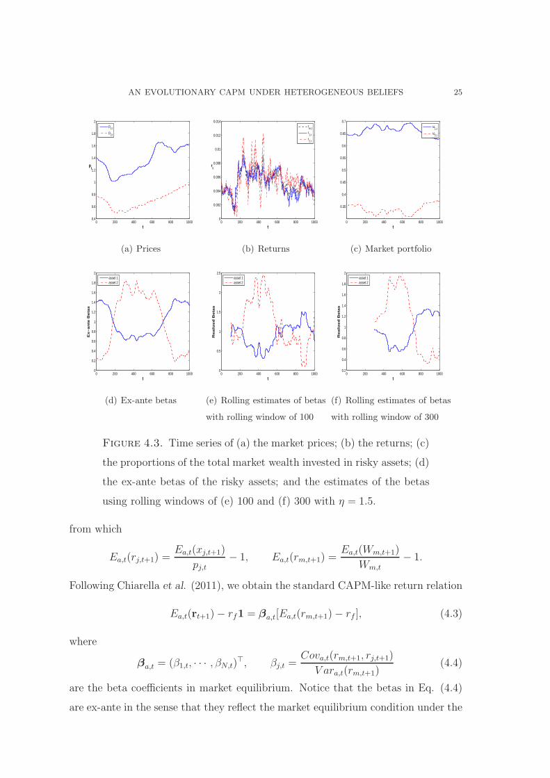
Figure 4.3. Time series of (a) the market prices; (b) the returns; (c)
the proportions of the total market wealth invested in risky assets; (d)
the ex-ante betas of the risky assets; and the estimates of the betas
using rolling windows of (e) 100 and (f) 300 with η = 1.5.
from which
Ea,t(rj,t+1) =Ea,t(xj,t+1)
pj,t− 1, Ea,t(rm,t+1) =
Ea,t(Wm,t+1)
Wm,t
− 1.
Following Chiarella et al. (2011), we obtain the standard CAPM-like return relation
Ea,t(rt+1)− rf1 = βa,t[Ea,t(rm,t+1)− rf ], (4.3)
where
βa,t = (β1,t, · · · , βN,t)⊤, βj,t =
Cova,t(rm,t+1, rj,t+1)
V ara,t(rm,t+1)(4.4)
are the beta coefficients in market equilibrium. Notice that the betas in Eq. (4.4)
are ex-ante in the sense that they reflect the market equilibrium condition under the
26 CHIARELLA, DIECI, HE AND LI
consensus belief Ea,t and Ωa,t. In addition, Eq. (4.2) also implies rm,t+1 = ω⊤t rt+1,
leading to ω⊤t βa,t = 1, where ωt = Pts/(p
⊤t s) with Pt = diag[p1,t, · · · , pN,t] are the
proportions of the total wealth (ex dividend) in the economy invested in the risky
assets at time t.
0 200 400 600 800 10000.2
0.4
0.6
0.8
1
1.2
1.4
1.6
1.8
t
pt
p
1,t
p2,t
(a) Prices
0 200 400 600 800 1000−2
0
2
4
6
8
10
12
14
16x 10
−3
t
rt
rm,t
r1,t
r2,t
(b) Returns
0 200 400 600 800 10000.25
0.3
0.35
0.4
0.45
0.5
0.55
0.6
0.65
0.7
0.75
t
ω
1,t
ω2,t
(c) Market portfolio
0 200 400 600 800 10000
0.5
1
1.5
2
2.5
3
t
Ex−
an
te B
eta
s
asset 1asset 2
(d) Ex-ante betas
0 200 400 600 800 10000
0.5
1
1.5
2
2.5
t
Re
aliz
ed
Be
tas
asset 1asset 2
(e) Rolling estimates of betas
with rolling window of 100
0 200 400 600 800 10000.2
0.4
0.6
0.8
1
1.2
1.4
1.6
1.8
2
t
Re
aliz
ed
Be
tas
asset 1asset 2
(f) Rolling estimates of betas
with rolling window of 300
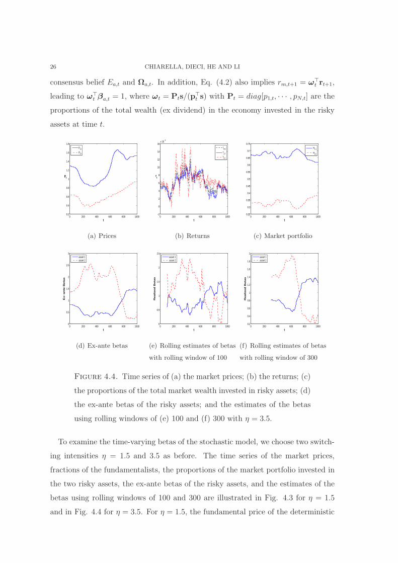
Figure 4.4. Time series of (a) the market prices; (b) the returns; (c)
the proportions of the total market wealth invested in risky assets; (d)
the ex-ante betas of the risky assets; and the estimates of the betas
using rolling windows of (e) 100 and (f) 300 with η = 3.5.
To examine the time-varying betas of the stochastic model, we choose two switch-
ing intensities η = 1.5 and 3.5 as before. The time series of the market prices,
fractions of the fundamentalists, the proportions of the market portfolio invested in
the two risky assets, the ex-ante betas of the risky assets, and the estimates of the
betas using rolling windows of 100 and 300 are illustrated in Fig. 4.3 for η = 1.5
and in Fig. 4.4 for η = 3.5. For η = 1.5, the fundamental price of the deterministic
AN EVOLUTIONARY CAPM UNDER HETEROGENEOUS BELIEFS 27
model is stable, the variation of the beta coefficients in Fig. 4.3 (d) is large but
less significant compared to the beta coefficients in Fig. 4.4 (d) for η = 3.5 (where
the fundamental price of the deterministic model is unstable). Both the pattern
and the level of the beta coefficients for η = 1.5 are very different from those for
η = 3.5. More importantly, both Figs. 4.3 and 4.4 show that the rolling estimates
of the betas do not necessarily reflect the nature of the ex-ante betas implied by the
CAPM, which is consistent with the results in Chiarella et al. (2012). Interestingly,
the estimated betas for window of 100 are more volatile compared to the ex-ante
betas. However, an increase in rolling window from 100 to 300 in (e) and (f) of Figs.
4.3 and 4.4 smooths the variations of the beta estimates significantly, leading to a
similar pattern to the ex-ante betas.
4.3. Trading Volume and Volatility. Finally, we examine the dynamic relation
between price volatility and trading volume. As in Banerjee and Kremer (2010),
the price volatility is measured by the price difference |pj,t − pj,t−1| and the trading
volume at time t is defined by
Xt =minnf,t−1, nf,t|zf,t − zf,t−1|+minnc,t−1, nc,t|zc,t − zc,t−1|
+ |nf,t − nf,t−1|Xt, (4.5)
where
Xt =
|zf,t − zc,t−1|, nf,t ≥ nf,t−1,
|zc,t − zf,t−1|, nf,t < nf,t−1.
Due to the switching mechanism, the total trading volume Xt in (4.5) can be de-
composed into three components. The first and second components correspond to
the trading volume of the agents who use, respectively, the fundamental and trend
following trading strategies at both time t − 1 and t. The third component corre-
sponds to the trading volume of those agents who change their strategies from t− 1
to t. In particular, when nf,t > nf,t−1, a fraction of nf,t − nf,t−1 agents change their
strategies from the trend following strategy at time t− 1 (with a demand of zc,t−1)
to the fundamental strategy at time t (with a demand of zf,t).
28 CHIARELLA, DIECI, HE AND LI
0 200 400 600 800 10000.8
0.9
1
1.1
1.2
1.3
1.4
1.5
1.6
1.7
1.8
t
p
1
p*1
(a) Prices of asset one
0 200 400 600 800 10000.8
0.9
1
1.1
1.2
1.3
1.4
1.5
t
p
2
p*2
(b) Prices of asset two
0 200 400 600 800 1000−0.2
−0.1
0
0.1
0.2
0.3
0.4
0.5
0.6
0.7
t
z
f,1
zc,1
s1+ξ
1
(c) The positions in asset one
0 200 400 600 800 1000−0.4
−0.3
−0.2
−0.1
0
0.1
0.2
0.3
0.4
t
z
f,2
zc,2
s2+ξ
2
(d) The positions in asset two
0 200 400 600 800 10000
2
4
6x 10
−3
|∆ p
1|
t
0 200 400 600 800 10000
0.1
0.2
0.3
Trad
ing
Vol
umes
|∆ p1|
Trading Volumes
(e) Volatility and volumes of asset one
0 200 400 600 800 10000
2
4x 10
−3
|∆ p
2|
t
0 200 400 600 800 10000
0.2
0.4
Trad
ing
Vol
umes
|∆ p2|
Trading Volumes
(f) Volatility and volumes of asset two
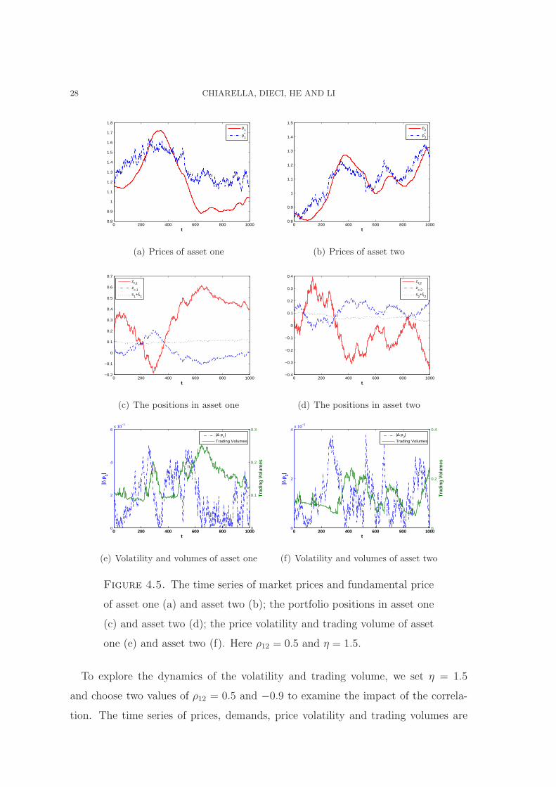
Figure 4.5. The time series of market prices and fundamental price
of asset one (a) and asset two (b); the portfolio positions in asset one
(c) and asset two (d); the price volatility and trading volume of asset
one (e) and asset two (f). Here ρ12 = 0.5 and η = 1.5.
To explore the dynamics of the volatility and trading volume, we set η = 1.5
and choose two values of ρ12 = 0.5 and −0.9 to examine the impact of the correla-
tion. The time series of prices, demands, price volatility and trading volumes are
AN EVOLUTIONARY CAPM UNDER HETEROGENEOUS BELIEFS 29
0 200 400 600 800 10001.4
1.6
1.8
2
2.2
2.4
2.6
2.8
t
p
1
p*1
(a) Prices of asset one
0 200 400 600 800 10002
2.2
2.4
2.6
2.8
3
3.2
3.4
t
p
2
p*2
(b) Prices of asset two
0 200 400 600 800 1000−0.4
−0.2
0
0.2
0.4
0.6
0.8
1
1.2
t
z
f,1
zc,1
s1+ξ
1
(c) The positions in asset one
0 200 400 600 800 1000−1
−0.5
0
0.5
1
1.5
2
t
z
f,2
zc,2
s2+ξ
2
(d) The positions in asset two
0 200 400 600 800 10000
2
4
6
8x 10
−3
|∆ p
1|
t
0 200 400 600 800 10000
0.2
0.4
0.6
0.8
Trad
ing
Vol
umes
|∆ p1|
Trading Volumes
(e) Volatility and volumes of asset one
0 200 400 600 800 10000
0.005
0.01
|∆ p
2|
t
0 200 400 600 800 10000
0.5
1
Trad
ing
Vol
umes
|∆ p2|
Trading Volumes
(f) Volatility and volumes of asset two
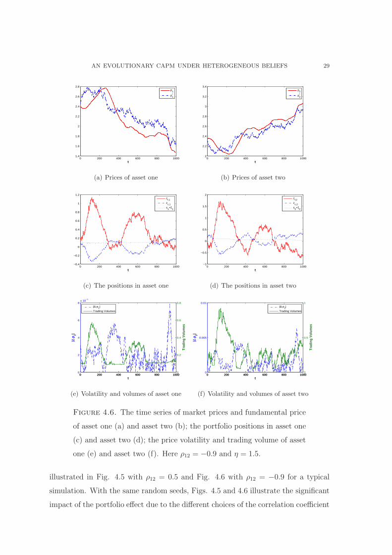
Figure 4.6. The time series of market prices and fundamental price
of asset one (a) and asset two (b); the portfolio positions in asset one
(c) and asset two (d); the price volatility and trading volume of asset
one (e) and asset two (f). Here ρ12 = −0.9 and η = 1.5.
illustrated in Fig. 4.5 with ρ12 = 0.5 and Fig. 4.6 with ρ12 = −0.9 for a typical
simulation. With the same random seeds, Figs. 4.5 and 4.6 illustrate the significant
impact of the portfolio effect due to the different choices of the correlation coefficient
30 CHIARELLA, DIECI, HE AND LI
0 20 40 60 80 1000
0.1
0.2
0.3
0.4
0.5
0.6
0.7
0.8
0.9
lag
AC
F( |∆
p1|)
(a) The ACs of the price volatility
0 20 40 60 80 1000
0.1
0.2
0.3
0.4
0.5
0.6
0.7
lag
AC
F(X
1)
(b) The ACs of the trading volume
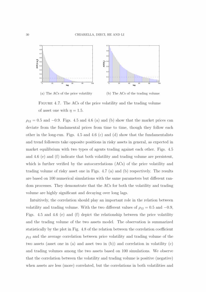
Figure 4.7. The ACs of the price volatility and the trading volume
of asset one with η = 1.5.
ρ12 = 0.5 and −0.9. Figs. 4.5 and 4.6 (a) and (b) show that the market prices can
deviate from the fundamental prices from time to time, though they follow each
other in the long-run. Figs. 4.5 and 4.6 (c) and (d) show that the fundamentalists
and trend followers take opposite positions in risky assets in general, as expected in
market equilibrium with two types of agents trading against each other. Figs. 4.5
and 4.6 (e) and (f) indicate that both volatility and trading volume are persistent,
which is further verified by the autocorrelations (ACs) of the price volatility and
trading volume of risky asset one in Figs. 4.7 (a) and (b) respectively. The results
are based on 100 numerical simulations with the same parameters but different ran-
dom processes. They demonstrate that the ACs for both the volatility and trading
volume are highly significant and decaying over long lags.
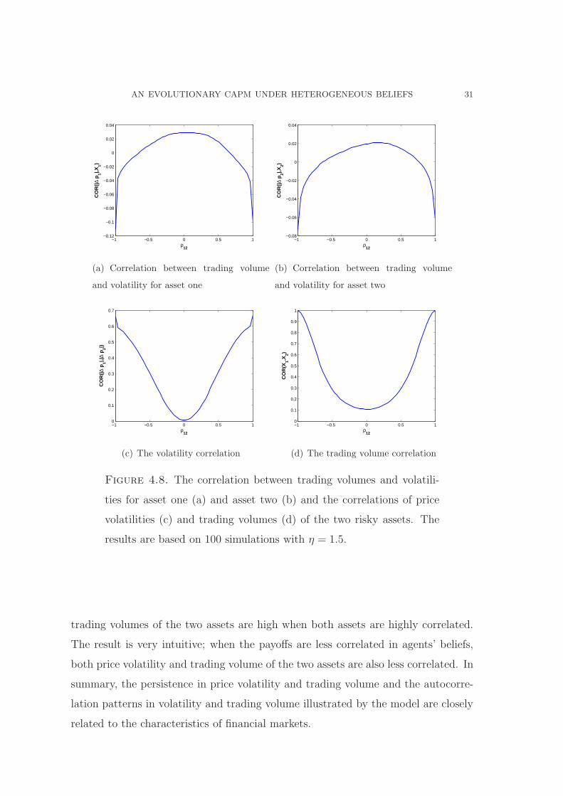
Intuitively, the correlation should play an important role in the relation between
volatility and trading volume. With the two different values of ρ12 = 0.5 and −0.9,
Figs. 4.5 and 4.6 (e) and (f) depict the relationship between the price volatility
and the trading volume of the two assets model. The observation is summarized
statistically by the plot in Fig. 4.8 of the relation between the correlation coefficient
ρ12 and the average correlation between price volatility and trading volume of the
two assets (asset one in (a) and asset two in (b)) and correlation in volatility (c)
and trading volumes among the two assets based on 100 simulations. We observe
that the correlation between the volatility and trading volume is positive (negative)
when assets are less (more) correlated, but the correlations in both volatilities and
AN EVOLUTIONARY CAPM UNDER HETEROGENEOUS BELIEFS 31
−1 −0.5 0 0.5 1−0.12
−0.1
−0.08
−0.06
−0.04
−0.02
0
0.02
0.04
ρ12
CO
R(|
∆ p
1|,X1)
(a) Correlation between trading volume
and volatility for asset one
−1 −0.5 0 0.5 1−0.08
−0.06
−0.04
−0.02
0
0.02
0.04
ρ12
CO
R(|
∆ p
2|,X2)
(b) Correlation between trading volume
and volatility for asset two
−1 −0.5 0 0.5 10
0.1
0.2
0.3
0.4
0.5
0.6
0.7
ρ12
CO
R(|
∆ p
1|,|∆
p2|)
(c) The volatility correlation
−1 −0.5 0 0.5 10
0.1
0.2
0.3
0.4
0.5
0.6
0.7
0.8
0.9
1
ρ12
CO
R(X
1,X2)
(d) The trading volume correlation
Figure 4.8. The correlation between trading volumes and volatili-
ties for asset one (a) and asset two (b) and the correlations of price
volatilities (c) and trading volumes (d) of the two risky assets. The
results are based on 100 simulations with η = 1.5.
trading volumes of the two assets are high when both assets are highly correlated.
The result is very intuitive; when the payoffs are less correlated in agents’ beliefs,
both price volatility and trading volume of the two assets are also less correlated. In
summary, the persistence in price volatility and trading volume and the autocorre-
lation patterns in volatility and trading volume illustrated by the model are closely
related to the characteristics of financial markets.
32 CHIARELLA, DIECI, HE AND LI
5. Conclusion
This paper extends the single-period equilibrium CAPM of Chiarella et al (2011)
to a dynamic equilibrium evolutionary CAPM to incorporate the adaptively switch-
ing behaviour of heterogeneous agents. By analyzing the stability of the underlying
deterministic model, we show that the evolutionary CAPM is capable of character-
izing the spill-over effects, the persistence in price volatility and trading volume,
and realistic correlations between price volatility and trading volume. Also, the sto-
chastic nature of time-varying betas implied by the equilibrium model may not be
consistent with the rolling window estimate of betas used in the empirical literature.
The model provides further explanatory power of the recently developed HAMs.
In this paper, the numerical analysis is focused on the case of two risky assets,
though the stability analysis is conducted for any number of risky assets. It would be
interesting to see how an increase in the number of risky assets could have different
effects. We expect the main results obtained in this paper to hold. The statistical
analysis is mainly based on some Monte Carlo simulations and a systematical study
of the empirical relevance using econometric methods would be interesting. We leave
these issues to the future research.
Appendix A. Proofs
To provide some insights into the proof of the model with many risky assets, we
first start with the case of one risky asset.
A.1. Proof of Proposition 3.2. In order to prove the local stability properties
of the deterministic model (3.1), we start from the simplified one-risky-asset case
(3.3). We omit the index j of the unique risky asset for simplicity.
Note that pt depends only on pt−1, ut−1, Vt−1, and on nf,t. The same holds
for the state variables ut and Vt. The differential of the fitness functions at time
t, v∆,t, depends on pt−2, ut−2, Vt−2 and pt−1 through the demand functions zf,t−1
and zc,t−1, on nf,t−1 through θa,t−1, as well as on pt, pt−1, pt−2 directly. Formally,
suitable changes of variables allow us to express the dynamical system (3.3) as an
8-dimensional map, by which the state of the system at time t is expressed as a
AN EVOLUTIONARY CAPM UNDER HETEROGENEOUS BELIEFS 33
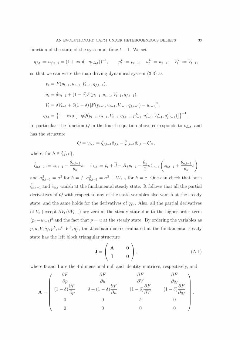
function of the state of the system at time t− 1. We set
qf,t := nf,t+1 = (1 + exp(−ηv∆,t))−1, pLt := pt−1, uL
t := ut−1, V Lt := Vt−1,
so that we can write the map driving dynamical system (3.3) as
pt = F (pt−1, ut−1, Vt−1, qf,t−1),
ut = δut−1 + (1− δ)F (pt−1, ut−1, Vt−1, qf,t−1),
Vt = δVt−1 + δ(1− δ) [F (pt−1, ut−1, Vt−1, qf,t−1)− ut−1]2 ,
qf,t =1 + exp
[−ηQ(pt−1, ut−1, Vt−1, qf,t−1, p
Lt−1, u
Lt−1, V
Lt−1, q
Lf,t−1)
]−1.
In particular, the function Q in the fourth equation above corresponds to v∆,t, and
has the structure
Q = v∆,t = ζf,t−1πf,t − ζc,t−1πc,t − C∆,
where, for h ∈ f, c,
ζh,t−1 := zh,t−1 −θa,t−1
θhs, πh,t := pt + d− Rfpt−1 −
θh2σ2h,t−1
(zh,t−1 +
θa,t−1
θhs
)
and σ2h,t−1 = σ2 for h = f , σ2
h,t−1 = σ2 + λVt−2 for h = c. One can check that both
ζh,t−1 and πh,t vanish at the fundamental steady state. It follows that all the partial
derivatives of Q with respect to any of the state variables also vanish at the steady
state, and the same holds for the derivatives of qf,t. Also, all the partial derivatives
of Vt (except ∂Vt/∂Vt−1) are zero at the steady state due to the higher-order term
(pt−ut−1)2 and the fact that p = u at the steady state. By ordering the variables as
p, u, V, qf , pL, uL, V L, qLf , the Jacobian matrix evaluated at the fundamental steady
state has the left block triangular structure
J =
A 0
I 0
, (A.1)
where 0 and I are the 4-dimensional null and identity matrices, respectively, and
A =
∂F
∂p
∂F
∂u
∂F
∂V
∂F
∂qf
(1− δ)∂F
∂pδ + (1− δ)
∂F
∂u(1− δ)
∂F
∂V(1− δ)
∂F
∂qf
0 0 δ 0
0 0 0 0
.

34 CHIARELLA, DIECI, HE AND LI
It follows that the characteristic equation for J is given by
χ5(χ− δ)(χ2 +m1χ+m2) = 0,
where16
m1 =α + δγ
Rf (1 + θ0eηC∆)−
δγ + 1
Rf
− δ, m2 = δ
[1 + γ
Rf
−α + γ
Rf(1 + θ0eηC∆)
].
As 0 < δ < 1, it follows that stability depends only on the roots of the 2nd-degree
polynomial χ2 +m1χ + m2. The latter represents the characteristic polynomial of
the two-dimensional upper-left block of matrix A (that we denote as B). A well-
known necessary and sufficient condition for both characteristic roots of B, say χ1
and χ2, to have modulus smaller than one (implying that the steady state is locally
asymptotically stable in our case) is the set of inequalities,
1 +m1 +m2 > 0, 1−m1 +m2 > 0, m2 < 1. (A.2)
The first and second inequalities of (A.2) always hold for any η ≥ 0. The third
condition is equivalent to
δ(1 + γ)−Rf <δ(α + γ)
1 + θ0eηC∆. (A.3)
If Rf ≥ δ(1+ γ), then condition (A.3) always holds for any η ≥ 0. If Rf < δ(1+ γ),
then (A.3) holds when η < η := 1C∆
lnRf−δ(1−α)
θ0[δ(1+γ)−Rf ]. If C∆ = 0, then Eq. (A.3) holds
whenRf−δ(1−α)
θ0[δ(1+γ)−Rf ]> 1, which is equivalent to θ0γ < α+(1+θ0)(
Rf
δ−1). This proves
Proposition 3.2.
A.2. Proof of Proposition 3.1. Consider the general case (3.1) of N risky
assets. The structure of the map is the same as in the simplified one-risky-asset
case, except that the variables pt, ut, pLt , u
Lt have dimension N , whereas Vt and
VLt have dimension M := N(N + 1)/2 (e.g. M = 3 for the two-asset case). Again,
p = u at the steady state, and the derivatives of each component of Vt in system
(3.1) with respect to any of the state variables (with the exception of Vt−1) vanish
16See later for the N -asset case with the computational details regarding∂F
∂pand
∂F
∂u.
AN EVOLUTIONARY CAPM UNDER HETEROGENEOUS BELIEFS 35
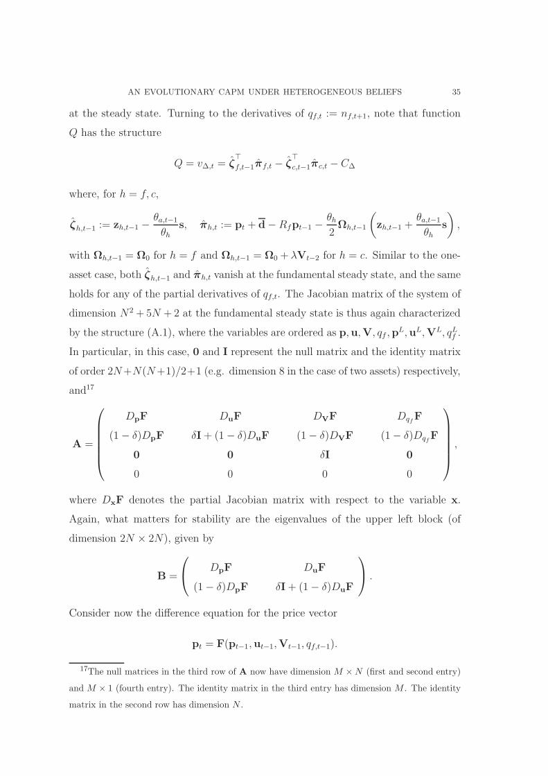
at the steady state. Turning to the derivatives of qf,t := nf,t+1, note that function
Q has the structure
Q = v∆,t = ζ⊤
f,t−1πf,t − ζ⊤
c,t−1πc,t − C∆
where, for h = f, c,
ζh,t−1 := zh,t−1 −θa,t−1
θhs, πh,t := pt + d−Rfpt−1 −
θh2Ωh,t−1
(zh,t−1 +
θa,t−1
θhs
),
with Ωh,t−1 = Ω0 for h = f and Ωh,t−1 = Ω0 + λVt−2 for h = c. Similar to the one-
asset case, both ζh,t−1 and πh,t vanish at the fundamental steady state, and the same
holds for any of the partial derivatives of qf,t. The Jacobian matrix of the system of
dimension N2 +5N +2 at the fundamental steady state is thus again characterized
by the structure (A.1), where the variables are ordered as p,u,V, qf ,pL,uL,VL, qLf .
In particular, in this case, 0 and I represent the null matrix and the identity matrix
of order 2N+N(N+1)/2+1 (e.g. dimension 8 in the case of two assets) respectively,
and17
A =
DpF DuF DVF DqfF
(1− δ)DpF δI+ (1− δ)DuF (1− δ)DVF (1− δ)DqfF
0 0 δI 0
0 0 0 0
,
where DxF denotes the partial Jacobian matrix with respect to the variable x.
Again, what matters for stability are the eigenvalues of the upper left block (of
dimension 2N × 2N), given by
B =
DpF DuF
(1− δ)DpF δI+ (1− δ)DuF
.
Consider now the difference equation for the price vector
pt = F(pt−1,ut−1,Vt−1, qf,t−1).
17The null matrices in the third row of A now have dimension M ×N (first and second entry)
and M × 1 (fourth entry). The identity matrix in the third entry has dimension M . The identity
matrix in the second row has dimension N .

36 CHIARELLA, DIECI, HE AND LI
The partial Jacobian with respect to p is given by
DpF =θa,tRf
Ωa,t
[qf,t−1
θfΩ−1
0 (I−α) +1− qf,t−1
θc(Ω0 + λVt−1)
−1(I+ γ)
]
where I is the N -dimensional identity matrix, α := diag(α1, α2, ..., αN) and
γ:=diag(γ1, γ2, ..., γN). At the steady state (where Ωa,t = Ω0) we obtain
DpF(p∗,p∗, 0,q∗f ) =
θ∗aRf
[n∗f
θf(I−α) +
1− n∗f
θc(I+ γ)
],
whereθ∗aθf
n∗
f =1
1 + θ0eηC∆,
θ∗aθc(1− n∗
f) =θ0e
ηC∆
1 + θ0eηC∆.
Note that DpF(p∗,p∗, 0,q∗f ) is a diagonal matrix. This implies that the fixed com-
ponent Ω0 of variance/covariance beliefs, in particular the correlations, has no effect
on the dynamics of the linearized system around the steady state. Similarly, one
obtains for DuF the expression
DuF(p∗,p∗, 0,q∗f ) = −
θ∗aRf
1− n∗f
θcγ,
which is also a diagonal matrix. Every submatrix of block B is therefore an N -
dimensional diagonal matrix. It follows that the characteristic equation of J is
given by
χ(N+1)(N+4)
2 (χ− δ)N(N+1)
2
N∏
j=1
(χ2 +m1,jχ +m2,j) = 0,
where in particular the characteristic equation of B is represented by the product
of the N 2nd-degree polynomials, and the coefficients m1,j and m2,j have the same
structure as those of the one-asset case, namely
m1,j =αj + δγj
Rf (1 + θ0eηC∆)−
δγj + 1
Rf
− δ, m2,j = δ
[1 + γjRf
−αj + γj
Rf(1 + θ0eηC∆)
].
Each of the above second-order polynomials is naturally associated with one of the
risky assets. The steady state (p∗,p∗, 0,q∗f) is thus locally asymptotically stable if
and only if, for all j ∈ 1, 2, ..., n,
1 +m1,j +m2,j > 0, 1−m1,j +m2,j > 0, m2,j < 1. (A.4)
Similar to the one-asset case, the first two inequalities hold for any η ≥ 0. The above
set of inequalities is thus satisfied for any η ≥ 0 if Rf ≥ δ(1+ γj). If Rf < δ(1+ γj),
it is satisfied only if η < ηj :=1
C∆ln
Rf−δ(1−αj )
θ0[δ(1+γj )−Rf ]or, in the particular case C∆ = 0,
AN EVOLUTIONARY CAPM UNDER HETEROGENEOUS BELIEFS 37
if θ0γj < αj + (1 + θ0)(Rf
δ− 1). Since stability requires that condition (A.4) holds
for all j ∈ 1, 2, ..., n, the statement of Proposition 3.1 follows.
References
Ang, A. and Chen, J. (2007), ‘CAPM over the long run: 1926 to 2001’, Journal of Empirical
Finance 14, 1–40.
Banerjee, S. and Kremer, I. (2010), ‘Disagreement and learning: dynamic patterns of trade’,
Journal of Finance 65, 1269–1302.
Bollerslev, T. (1986), ‘Generalized autoregressive conditional heteroskedasticity’, Journal of Econo-
metrics 31, 307–327.
Bollerslev, T., Engle, R. and Wooldridge, J. (1988), ‘A capital asset pricing model with time
varying covariances’, Journal of Political Economy 96, 116–131.
Braun, P., Nelson, D. and Sunier, A. (1990), ‘Good news, bad news, volatility and betas’, Journal
of Finance 50, 1575–1603.
Brock, W. and Hommes, C. (1997), ‘A rational route to randomness’, Econometrica 65, 1059–1095.
Brock, W. and Hommes, C. (1998), ‘Heterogeneous beliefs and routes to chaos in a simple asset
pricing model’, Journal of Economic Dynamics and Control 22, 1235–1274.
Campbell, J. and Vuolteenaho, T. (2004), ‘Bad beta, good beta’, American Economic Review
94(5), 1249–1275.
Chen, S.-H. and Huang, Y. (2008), ‘Risk preference, forecasting accuracy and survival dynamics:
simulations based on a multi-asset agent-based artifical stock market’, Journal of Economic
Behavior and Organization 67, 702–717.
Chiarella, C., Dieci, R. and Gardini, L. (2005), ‘The dynamic interaction of speculation and diver-
sification’, Applied Mathematical Finance 12(1), 17–52.
Chiarella, C., Dieci, R. and He, X. (2009), Heterogeneity, Market Mechanisms and Asset Price
Dynamics, Elsevier, pp. 277–344. in Handbook of Financial Markets: Dynamics and Evolution,
Eds. Hens, T. and K.R. Schenk-Hoppe.
Chiarella, C., Dieci, R. and He, X. (2010), A framework for CAPM with heterogeneous beliefs,
Springer, pp. 353–369. in Nonlinear Dynamics in Economics, Finance and Social Sciences:
Essays in Honour of John Barkley Rosser Jr., Eds. Bischi, G.-I., C. Chiarella and L. Gardini.
Chiarella, C., Dieci, R. and He, X. (2011), ‘Do heterogeneous beliefs diversify market risk?’, Euro-
pean Journal of Finance 17(3), 241–258.
Chiarella, C., Dieci, R. and He, X. (2012), ‘Time-varying beta: A boundedly rational equilibrium
approach’, Journal of Evolutionary Economics . to appear (DOI 10.1007/s00191-011-0233-5).
Chiarella, C., He, X. and Zheng, M. (2011), ‘An analysis of the effect of noise in a heterogeneous
agent financial market model’, Journal of Economic Dynamics and Control 35. 148-162.
38 CHIARELLA, DIECI, HE AND LI
Dieci, R. and Westerhoff, F. (2010a), ‘Heterogeneous speculators, endogenous fluctuations and
interacting markets: A model of stock prices and exchange rates’, Journal of Economic Dy-
namics and Control 34, 743–764.
Dieci, R. and Westerhoff, F. (2010b), On the inherent instability of international financial markets:
natural nonlinear interactions between stock and foreign exchange markets, BERG (Bam-
berg Economic Research Group) on Government and Growth Working Paper Series, no. 79,
University of Bamberg.
Dybvig, P. and Ross, S. (1985), ‘Differential information and performance measurement using a
security market line’, Journal of Finance 40, 383–400.
Engle, R. (1982), ‘Autoregressive conditional heteroscedasticity with estimates of the variance of
UK inflation’, Econometrica 50, 987–1008.
Evstigneev, I., Hens, T. and Schenk-Hoppe, K.R. (2009), Evolutionary Finance, Elsevier, pp. 507–
566. in Handbook of Financial Markets: Dynamics and Evolution, Eds. Hens, T. and K.R.
Schenk-Hoppe.
Fama, E. and French, K. (2006), ‘The value premium and the CAPM’, Journal of Finance
61(5), 2163–2185.
Hamilton, J. (1989), ‘A new approach to the economic analysis of nonstationary time series and
the business cycle’, Econometrica 57(2), 357–384.
Hamilton, J. (1990), ‘Analysis of time series subject to changes in regime’, Journal of Econometrics
45, 39–70.
Hansen, L. and Richard, S. (1987), ‘The role of conditioning information in deducing testable
restrictions implied by dynamic asset pricing models’, Econometrica 55, 587–613.
He, X. and Li, Y. (2007), ‘Power law behaviour, heterogeneity, and trend chasing’, Journal of
Economic Dynamics and Control 31, 3396–3426.
Hens, T. and Schenk-Hoppe, K. R., eds (2009), Handbook of Financial Markets: Dynamics and
Evolution, Handbooks in Finance, Elsevier.
Hommes, C. (2001), ‘Financial markets as nonlinear adaptive evolutionary systems’, Quantitative
Finance 1, 149–167.
Hommes, C. (2006), Heterogeneous Agent Models in Economics and Finance, Vol. 2 of Handbook
of Computational Economics, North-Holland, pp. 1109–1186. in Agent-based Computational
Economics, Eds. Tesfatsion, L. and K.L. Judd.
Hommes, C. and Wagener, F. (2009), Complex Evolutionary Systems in Behavioral Finance, Chap-
ter 4 in ‘Handbooks in Finance’, North-Holland, pp. 217–276. in Handboof of Financial Mar-
kets: Dynamics and Evolution, Eds. Hens, T. and K.R. Schenk-Hoppe.
Jagannathan, R. and Wang, Z. (1996), ‘The conditional CAPM and cross-section of expected
returns’, Journal of Finance 51, 3–53.
AN EVOLUTIONARY CAPM UNDER HETEROGENEOUS BELIEFS 39
LeBaron, B. (2006), Agent-based Computational Finance, Vol. 2 of Handbook of Computational
Economics, North-Holland, pp. 1187–1233. in Agent-based Computational Economics, Eds.
Tesfatsion, L. and K.L. Judd.
Lewellen, J. and Nagel, S. (2006), ‘The conditional CAPM does not explain asset-pricing anom-
alies’, Journal of Financial Economics 82(3), 289–314.
Lintner, J. (1965), ‘The valuation of risk assets and the selection of risky investments in stock
portfolios and capital budgets’, Review of Economic Studies 47, 13–37.
Lux, T. (2009), Stochastic Behavioural Asset Pricing and Stylized Facts, Elsevier, pp. 161–215. in
Handbook of Financial Markets: Dynamics and Evolution, Eds. Hens, T. and K.R. Schenk-
Hoppe.
Marsili, M., Raffaelli, G. and Ponsot, B. (2009), ‘Dynamic instability in generic model of multi-
assets markets’, Journal of Economic Dynamics and Control 33, 1170–1181.
Mossin, J. (1966), ‘Equilibrium in a capital asset market’, Econometrica 35, 768–783.
Sharpe, W. (1964), ‘Capital asset prices: A theory of market equilibrium under conditions of risk’,
Journal of Finance 19, 425–442.
Westerhoff, F. (2004), ‘Multiasset market dynamics’, Macroeconomic Dynamics 8, 591–616.
Westerhoff, F. and Dieci, R. (2006), ‘The effectiveness of Keynes-Tobin transaction taxes when
heterogeneous agents can trade in different markets: A behavioral finance approach’, Journal
of Economic Dynamics and Control 30, 293–322.
Zhu, M., Wang, D. and Guo, M. (2011), ‘Stochastic equilibria of an asset pricing model with
heterogeneous beliefs and random dividends’, Journal of Economic Dynamics and Control
35, 131–147.