quantifying heteroskedasticity metrics - home -...
TRANSCRIPT
DEAKIN UNIVERSITY
Quantifying Heteroskedasticity Metrics
by
Marwa Hassan Aly Hassan
A thesis submitted in fulfilment for the
degree of Doctorate of Philosophy
In the
Faculty of Science and Technology
Institute for Intelligent Systems Research and Innovation (IISRI)
November 2016


Abstract
Heteroskedasticity is a statistical term that describes the differing variances of the
error terms in a time series dataset. The presence of heteroskedasticity in data
imposes serious challenges to different forecasting models. The lack of information
and accuracy of the available information can be overwhelming to the decision
maker, leading to many types of uncertainties. Heteroskedasticity of the data
affects the relationship between the predictor variable and the outcome. This
leads to false positive and false negative decisions in the hypothesis testing, and
invalidates the results of statistical tests.
The available approaches for studying heteroskedasticity, developed thus far, adopt
the strategy of accommodating heteroskedasticity in the time series and consider
it to be an inevitable source of noise. In these solutions, two forecasting models
are prepared for normal and heteroskedastic scenarios and a statistical test is to
determine whether or not the data is heteroskedastic. Practically, however, it has
been observed that time series data such as S&P 500 Index (financial time series),
has no homogeneity of variance over time. Consequently, if one assumes that the
data is homoskedastic when it is indeed heteroskedastic, then the regression model
2
3
assumptions (Gauss-Markov assumptions) will be violated. When this violation
occurs, the ordinary least squares estimates will not feature a minimum variance.
Moreover, one will not be able to determine if the estimated variances are too large
or too small. Thus, heteroskedasticity results in a violation of the Gauss-Markov
assumptions, and it needs to be rectified.
This study takes the heteroskedasticity tests to the next level and proposes a quan-
tification measure of heteroskedasticity in the time series. In this study, two meth-
ods are introduced for quantifying heteroskedasticity, namely Slope of Local Vari-
ance Index (SoLVI) and a statistical divergence method using the Bhattacharya
coefficient. Based on the experiments, both the Bhattacharrya divergence and
Slope of Local Variance (SoLVI) heteroskedasticity measures provide a quantifi-
able measure of heteroskedasticity. Both metrics maintain a lower and asymptotic
upper bound. The proposed measures can identify how heteroskedastic the data
is and how far the dataset under investigation is from being homoskedastic. The
introduced measures can identify for how long the data can be homoskedastic,
which can help in designing a prediction interval for the time series being exam-
ined. The proposed measurements are obtained by calculating the local variances
using linear filters, estimating variance trends, calculating the changes in variance
slopes, and finally obtaining the average slope angles. Data were drawn from series
of theoretical and real data sets. Finally, the proposed measures showed reliability
in measuring and quantifying heteroskedasticity in comparison to the hypothesis
and numerical tests of heteroskedasticity.
List of Publications
1. Hassan, M. and Hossny, M. and Nahavandi, S. and Creighton, D.; “Quantifying
Heteroskedasticity Using Slope of Local Variances Index,” Proceedings of the 15th
International Conference on Computer Modelling and Simulation, 2013.
2. Hassan, M. and Hossny, M. and Nahavandi, S. and Creighton, D.; “Quantifying
Heteroskedasticity via Binary Decomposition,” Proceedings of the 15th Interna-
tional Conference on Computer Modelling and Simulation, 2013.
3. Hassan, M. and Hossny, M. and Nahavandi, S. and Creighton, D.; “Het-
eroskedasticity Variance Index,” Proceedings of the 14th International Conference
on Computer Modelling and Simulation, 2012.
4. Hassan, M. and Hossny, M. and Nahavandi, S. and Creighton, D.; ” Quantifying
Heteroskedasticity via Statistical Divergence Measure,” Submitted to Economics
Letters on the 23rd of June, 2016.
5. Hassan, M. and Hossny, M. and Nahavandi, S. and Creighton, D.; ” Quantifying
Heteroskedasticity,” Submitted to IEEE Systems Journal on the 24th of June,
2016.
4

Research Contributions
This research introduces two novel approaches to quantify heteroskedasticity.
Local Variance Estimation methods use the definition of heteroskedasticity
as time-varying variance and derives an estimation of local variances in the time
series. SoLVI is introduced to quantify heteroskedasticity. Two variations were
developed in this method, variance of variance and slope of local variances. A
variance of local variances gives a reasonable estimate but suffers from a quadratic
growth and provides unbounded function. The slope of local variances solves both
problems.
Statistical Divergence methods investigate heteroskedasticity from a different
view point. These methods operate under the assumption that for a time series to
be heteroskedastic, the estimated local variances must follow a uniform distribu-
tion. Therefore, a statistical distribution for the estimated local variances is de-
rived and measured the distance between the derived distribution and the uniform
distribution using statistical divergence measures. The Bhattacharyya coefficient
is selected as the divergence metric as it reduced computational complexity and
asymptotic upper-bound.
5
Acknowledgements
Deepest gratitude and immeasurable appreciation for the help and support to make this
study possible and make this dream come true are extended to the following persons:
Professor Saeid Nahavandi: for offering me the opportunity to pursue my academic
dream
Associate Professor Douglas Creighton: for his help and support through this emotional
journey, with words of advice and encouragement
Dr Mohammed Hossny: for his time, help and support with coding, data and priceless
advice
Miss Trish O’Toole: for always making IISRI a home away from home
All the library staff at Deakin University: for keeping us updated with the latest research
in the field
6
Contents
Declaration of Authorship 1
Abstract 2
List of Publications 4
Research Contributions 5
Acknowledgements 6
List of Figures 10
1 Introduction 1
1.1 Overview . . . . . . . . . . . . . . . . . . . . . . . . . . . . . . . . . . . . 1
1.2 Motivation . . . . . . . . . . . . . . . . . . . . . . . . . . . . . . . . . . . 4
1.3 Scope and Assumptions . . . . . . . . . . . . . . . . . . . . . . . . . . . . 5
1.4 Thesis Outline . . . . . . . . . . . . . . . . . . . . . . . . . . . . . . . . . 6
2 Heteroskedasticity in Time Series 7
2.1 Time Series Data Sets . . . . . . . . . . . . . . . . . . . . . . . . . . . . . 7
2.1.1 Continuous and Discrete Data Sets . . . . . . . . . . . . . . . . . . 8
2.1.2 Stationary and Non-Stationary Data Sets . . . . . . . . . . . . . . 8
2.1.3 Deterministic and Stochastic Data Sets . . . . . . . . . . . . . . . 9
2.2 Time Series Analysis . . . . . . . . . . . . . . . . . . . . . . . . . . . . . . 10
2.2.1 Descriptive Analysis . . . . . . . . . . . . . . . . . . . . . . . . . . 12
2.2.2 Spectral Analysis . . . . . . . . . . . . . . . . . . . . . . . . . . . . 12
2.2.3 Explanative Analysis . . . . . . . . . . . . . . . . . . . . . . . . . . 13
2.2.4 Forecasting . . . . . . . . . . . . . . . . . . . . . . . . . . . . . . . 13
2.2.5 Intervention or Control Analysis . . . . . . . . . . . . . . . . . . . 14
2.2.6 ARMA-ARIMA Time Series Forecasting Techniques . . . . . . . . 15
2.3 ARCH Model . . . . . . . . . . . . . . . . . . . . . . . . . . . . . . . . . . 19
2.4 GARCH model . . . . . . . . . . . . . . . . . . . . . . . . . . . . . . . . . 22
2.4.1 GARCH modelling . . . . . . . . . . . . . . . . . . . . . . . . . . . 23
2.4.2 Restrictions on GARCH model . . . . . . . . . . . . . . . . . . . . 27
2.4.3 Outliers in GARCH model . . . . . . . . . . . . . . . . . . . . . . 28
2.5 Heteroskedasticity Challenges and Tests . . . . . . . . . . . . . . . . . . . 30
2.5.1 Heteroskedasticity Detection . . . . . . . . . . . . . . . . . . . . . 31
2.5.2 The Goldfeld-Quandt test . . . . . . . . . . . . . . . . . . . . . . . 33
7
Contents 8
2.5.3 Ordinary likelihood ratio test . . . . . . . . . . . . . . . . . . . . . 34
2.5.4 Conditional likelihood ratio test . . . . . . . . . . . . . . . . . . . 34
2.5.5 Modified likelihood ratio test . . . . . . . . . . . . . . . . . . . . . 35
2.5.6 Residual likelihood ratio test . . . . . . . . . . . . . . . . . . . . . 36
2.5.7 Breusch-Pagan Test . . . . . . . . . . . . . . . . . . . . . . . . . . 36
2.5.8 White Test . . . . . . . . . . . . . . . . . . . . . . . . . . . . . . . 38
2.5.9 Levene’s Test . . . . . . . . . . . . . . . . . . . . . . . . . . . . . . 39
2.5.10 Spearman’s Rank Correlation Coefficient . . . . . . . . . . . . . . 40
2.5.11 Heteroskedasticity challenges . . . . . . . . . . . . . . . . . . . . . 41
2.6 Conclusions . . . . . . . . . . . . . . . . . . . . . . . . . . . . . . . . . . . 42
3 Critical Review of the Literature 44
3.1 ARCH model . . . . . . . . . . . . . . . . . . . . . . . . . . . . . . . . . . 44
3.2 GARCH model . . . . . . . . . . . . . . . . . . . . . . . . . . . . . . . . . 48
3.2.1 GARCH modelling . . . . . . . . . . . . . . . . . . . . . . . . . . . 49
3.2.2 Restrictions on GARCH model . . . . . . . . . . . . . . . . . . . . 52
3.2.3 Outliers in GARCH modeling . . . . . . . . . . . . . . . . . . . . . 53
3.3 Prediction Interval Modelling . . . . . . . . . . . . . . . . . . . . . . . . . 55
3.4 Conclusions . . . . . . . . . . . . . . . . . . . . . . . . . . . . . . . . . . . 57
4 SoLVI: Slope of Local Variance Index 59
4.1 Local Estimation of Statistical Parameters . . . . . . . . . . . . . . . . . . 60
4.1.1 Estimation of Local Average . . . . . . . . . . . . . . . . . . . . . 60
4.1.2 Generalisation with Gaussian Filters . . . . . . . . . . . . . . . . . 62
4.1.3 Estimation of Local Variance . . . . . . . . . . . . . . . . . . . . . 62
4.1.4 ARMA Filter . . . . . . . . . . . . . . . . . . . . . . . . . . . . . . 63
4.2 HVI: Heteroskedasticity Variance Index . . . . . . . . . . . . . . . . . . . 66
4.3 SoLVI: Slope of Local Variance Index . . . . . . . . . . . . . . . . . . . . . 68
4.3.1 Local Variance Regression . . . . . . . . . . . . . . . . . . . . . . . 69
4.3.2 Average Slope of Local Variance . . . . . . . . . . . . . . . . . . . 70
4.3.3 Selection of Kernel Size w . . . . . . . . . . . . . . . . . . . . . . . 71
4.4 Conclusions . . . . . . . . . . . . . . . . . . . . . . . . . . . . . . . . . . . 71
5 Divergence Heteroskedasticity Measure 73
5.1 Mutual Information (MI) . . . . . . . . . . . . . . . . . . . . . . . . . . . 74
5.1.1 Tsallis Driven Mutual Information (MIα) . . . . . . . . . . . . . . 76
5.2 Jensen-Shannon Divergence . . . . . . . . . . . . . . . . . . . . . . . . . . 76
5.3 Renyi Divergence . . . . . . . . . . . . . . . . . . . . . . . . . . . . . . . . 77
5.4 Bhattacharyya Distance . . . . . . . . . . . . . . . . . . . . . . . . . . . . 78
5.4.1 Hellinger Distance . . . . . . . . . . . . . . . . . . . . . . . . . . . 81
5.4.2 Bhattacharyya Heteroskedasticity Measure . . . . . . . . . . . . . 81
5.5 Conclusions . . . . . . . . . . . . . . . . . . . . . . . . . . . . . . . . . . . 82
6 Conclusions and Future Work 84

Contents 9
References 87
List of Figures
1.1 A comparison between homoskedastic and heteroskedastic data. . . 4
2.1 A comparison between stationary and non-stationary time-series. . 92.2 Fat-tailing Phenomenon. . . . . . . . . . . . . . . . . . . . . . . . . 10
4.1 Local variances of homoskedastic and heteroskedastic samples. . . . 644.2 Local variances of a heteroskedastic time series using convolution. . 654.3 Local variances of a heteroskedastic time series using autoregression. 664.4 Local variance comparison using convolution and autoregressive fil-
tering. . . . . . . . . . . . . . . . . . . . . . . . . . . . . . . . . . . 674.5 HVI with different kernel sizes . . . . . . . . . . . . . . . . . . . . . 684.6 SolVI scores for time series generated using different 64 sigmas. The
graphs demonstrate different kernel sizes w. . . . . . . . . . . . . . 70
5.1 Probability density function of local variances for homoskedasticand heteroskedastic time series . . . . . . . . . . . . . . . . . . . . . 73
5.2 The effect of HVI window size on Bhattacharyya coefficient. Theresult are of time series generated using different 64 sigmas. Thegraphs demonstrate different kernel sizes w. . . . . . . . . . . . . . 79
5.3 Bhattacharyya distance of a time series generated using different 64sigmas. The graphs demonstrate different kernel sizes w. . . . . . . 80
5.4 Hellinger coeffecient of a time series generated using different 64sigmas. The graphs demonstrate different kernel sizes w. . . . . . . 82
10

To my Dad: I am everything I am today because you loved me.
Thank you for being my father. Hope I made you proud.
My Mum : Thank you for always believing in me, always pushing
me towards success every single day.
My brothers, Mohammed and Mostafa: Thank you for being my
support and my rock when it gets hard along the way.
My Husband, Mohammed: words cannot describe how grateful I
am. Thank you for making my dream come true. And above all,
thank you for joining me in this journey.
My beautiful boys, Ahmed and Omar: You are the reason I wake
up every morning determined to be the best I can be. Thank you
for being the joy of my life. Love you to infinity and beyond.
11
Chapter 1
Introduction
1.1 Overview
Statistical uncertainty is defined as a lack of knowledge. This lack of knowledge,
either of information or in the context, can cause model-based predictions to devi-
ate from reality [1–3]. Some researchers have linked uncertainty to risk, due to the
lack of information or the lack of control [4–6]. This resulted in the assumption
that: to minimise the risk, the decision maker has to minimise uncertainty. On
the other hand, other researchers did not link uncertainty and risk, claiming they
are two different concepts. This led to two different scenarios: either uncertainty
depends on risk, or the other way around, risk depends on uncertainty.
Researchers have developed many strategies to deal with uncertainties. These
strategies range from simply ignoring the presence of the uncertainties, generat-
ing the missing knowledge causing uncertainties, interaction through communica-
tion, negotiation and dialogical learning, and finally applying the coping strategy
[5, 7, 8]. Uncertainty can be classified according to its predictability into: Aleatory
1

Introduction 2
and Epistemic uncertainties. Aleatory uncertainty is this type of uncertainty
that is caused by sudden disruption. This type of uncertainty is usually formu-
lated by probability distribution. Aleatory uncertainty is objective, stochastic and
irreducible [5, 7, 9–11]. Epistemic uncertainty is a predictable uncertainty be-
cause it results from missing or confusing knowledge. This can be detected at
the simulation or runtime phases [6, 12, 13]. The system performance can be im-
proved by increasing the knowledge and information. Epistemic uncertainty can
be classified into: model uncertainty, parametric uncertainty and completeness un-
certainty. Model uncertainty includes structural uncertainty, which is formulated
using geometric modelling and behavioural uncertainty formulated using algebraic
models. Parametric uncertainty is the type of uncertainty where the parameters
are known and predictable. It includes possible inaccuracies, due to small data
sets. Finally, completeness uncertainty is identifiable when some of the significant
properties and parameters are not studied in either uncertainty or risk analysis.
Uncertainty can be classified into logical uncertainty, mathematical uncertainty,
probability uncertainty and fuzzy logic. In this research, we are interested in
probability uncertainty. It is represented in the confidence intervals. The main
idea is to formulate a prediction interval that can represent the future based on
the examined data [6, 13].
A heteroskedastic time series features unpredictable measures of dispersion. This
uncertainty in statistical distribution parameters imposes a serious challenge to
Introduction 3
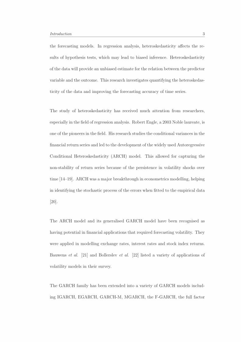
the forecasting models. In regression analysis, heteroskedasticity affects the re-
sults of hypothesis tests, which may lead to biased inference. Heteroskedasticity
of the data will provide an unbiased estimate for the relation between the predictor
variable and the outcome. This research investigates quantifying the heteroskedas-
ticity of the data and improving the forecasting accuracy of time series.
The study of heteroskedasticity has received much attention from researchers,
especially in the field of regression analysis. Robert Engle, a 2003 Noble laureate, is
one of the pioneers in the field. His research studies the conditional variances in the
financial return series and led to the development of the widely used Autoregressive
Conditional Heteroskedasticity (ARCH) model. This allowed for capturing the
non-stability of return series because of the persistence in volatility shocks over
time [14–19]. ARCH was a major breakthrough in econometrics modelling, helping
in identifying the stochastic process of the errors when fitted to the empirical data
[20].
The ARCH model and its generalised GARCH model have been recognised as
having potential in financial applications that required forecasting volatility. They
were applied in modelling exchange rates, interest rates and stock index returns.
Bauwens et al. [21] and Bollerslev et al. [22] listed a variety of applications of
volatility models in their survey.
The GARCH family has been extended into a variety of GARCH models includ-
ing IGARCH, EGARCH, GARCH-M, MGARCH, the F-GARCH, the full factor

Introduction 4
0 200 400 600 800 1000 1200 1400 1600 1800 2000
−30
−20
−10
0
10
20
30
40
sample at time t
y(t)
(a) Homoskedastic
0 200 400 600 800 1000 1200 1400 1600 1800 2000
−30
−20
−10
0
10
20
30
40
sample at time t
y(t)
(b) Heteroskedastic
Figure 1.1: A comparison between homoskedastic and heteroskedastic data. a) Ho-moskedastic (constant variance) sample. b) Heteroskedastic (varying variance).
FF-GARCH model, the orthogonal O-GARCH. ARCH and GARCH models are
important because they are widely used in econometrics and finance and they have
general applications. Based on the literature, ARCH and GARCH specifications
of errors and heteroskedasticity of data allow for a more accurate and reliable way
in forecasting volatility [2, 22–30]. Each of the previously listed models have en-
riched the literature of statistical and regression analysis with methods by which
to address the features of time series data for a better presentation. They also
aim to solve such problems in a more comprehensive way.
1.2 Motivation
A variety of statistical tests has been developed over the past three decades to de-
termine whether or not time series feature heteroskedastic behaviour. Regression
analysis, Monte Carlo and other simulation techniques were developed to minimise
the effect of uncertainty on decision-making. Yet, these tests cannot measure the
Introduction 5
degree of heteroskedasticity in the data, which can be valuable when developing a
long-term plan and decision-making. However, the monotonically increasing fre-
quency of global challenges such as economic crises, climate change and epidemics
highlighted the limitations of relying on hypothesis testing with binary results and
justified the need for quantifiable measures for heteroskedasticity. These measures,
however, must satisfy few constraints such as a zero-valued lower bound to indicate
homoskedasticity and an asymptotic upper bound for heteroskedasticity.
There have been many attempts to detect the heteroskedasticity in time series.
However, these tests do not quantify the amount of heteroskedasticity in the ex-
amined datasets. On the other hand, quantifying heteroskedasticity can provide
extra information about the behaviour of time series. Studying this behaviour will
improve forecasting of behavioural dependent time series data.
This research addresses the need to investigate the heteroskedasticity of the data,
the stationarity and the non-stationarity of the time series being tested and finally,
introducing a measure that can quantify heteroskedasticity.
1.3 Scope and Assumptions
This research focuses on error variance or linear regression models described by
Guass-Markov theorem in [31]. Consequently the Guass-Markov assumptions
state that the errors are uncorrellated and have an equal variance over time (ho-
moskedasticity) as follows.

Introduction 6
E (ui|x1, . . . , xn) = 0 (1.1)
V ar (ui|x1, . . . , xn) = σ2u, where 0 < σ2
u < ∞ (1.2)
E (uiuj|x1, . . . , xn) = 0, i �= j (1.3)
1.4 Thesis Outline
This research is structured as follows: Chapter 2 will address heteroskedasticity
in time series. It discusses time series data sets and the types of time series
analysis. In addition, we discuss the heteroskedasticity literature, how to deal with
heteroskedasticity of the data and its implications on the data analysis of different
models addressing heteroskedasticity, and the advantages and disadvantages of
these models. The available solutions are discussed and critically reviewed in
Chapter 3.
Chapter 4 investigates an approach to quantify heteroskedasticity and explores
the advantages and limitations of the proposed Heteroskedasticity Variance Index
(HVI) model. The experiments and test results will be illustrated and discussed.
The Slope of Local Variance Index (SoLVI) model will be introduced.
Chapter 5 introduces the Bhattacharyya Heteroskedasticity measure, that relies
on the Bhattacharya distance and coefficient metrics. Finally, the conclusions and
areas of future work are discussed in Chapter 6.
Chapter 2
Heteroskedasticity in Time Series
Time series analysis is defined as the analysis of observations with equal time in-
tervals. Fields of interest include statistics, signal processing, economics, financial
analysis, earthquake prediction and weather forecast. These time series are char-
acterised by exhibiting various degrees of correlation and/or volatility clustering
over time [32]. More statisticians are devoted to refining the existing models and
introducing new ones. Their goal is to provide the best models to meet today’s
complex tasks. Let us start our journey by expanding our definition of time series
analysis, its methods, and the types of data that it represents.
2.1 Time Series Data Sets
Another consideration when studying time series analysis is to understand the
various types of time series data sets. Time series data has specific characteristics
that affect long-term planning and forecasting. The main target of analysing
time series is to construct a prediction interval. This prediction interval aims
to predict future values of the series. They are classified into three categories:
7

Heteroskedasticity in Time Series 8
Continuous versus Discrete time series, Stationary versus Non stationary, and
finally Deterministic versus Stochastic time series [33, 34].
2.1.1 Continuous and Discrete Data Sets
Continuous time series is when the behaviour of a system is described by a set
of linear differential equations. Continuous models are represented with f(t) and
the changes in the data are always reflected over continuous time intervals. On
the other hand, the Discrete time series is when the behaviour is described by
difference equations. A difference equation, is also known as ”recurrence relation”.
The recurrence relation is an equation described as a function of the preceding term
as a sequence. A discrete model does not take into consideration the function of
time.
2.1.2 Stationary and Non-Stationary Data Sets
A stationary time series is when the data fluctuates around a constant time. It is
a stochastic process with a joint probability distribution kept constant at all time-
intervals. Non-stationary time series is when the parameters of the series (length,
amplitude and phase) change over time. The joint probability distribution of
non-stationary process is dependent on the time index. The trends need to be
eliminated to avoid their impacts on the other features of the time series data.

Heteroskedasticity in Time Series 9
0 1000 2000 3000 4000 5000 6000 7000 8000 9000 100000
20
40
60
80
100
120
sample (t)
read
ings
y(t
)
time series data y(t)local std dev σ
y(t)
(a) Time Invariant Mean and Variance
0 1000 2000 3000 4000 5000 6000 7000 8000 9000 10000−40
−20
0
20
40
60
80
100
120
140
sample (t)
read
ings
y(t
)
time series data y(t)local std dev σ
y(t)
(b) Time Variant Mean
0 1000 2000 3000 4000 5000 6000 7000 8000 9000 10000−1500
−1000
−500
0
500
1000
1500
2000
sample (t)
read
ings
y(t
)
time series data y(t)local std dev σ
y(t)
(c) Time Variance Variance)
0 1000 2000 3000 4000 5000 6000 7000 8000 9000 10000−50
0
50
100
150
200
250
300
350
400
sample (t)
read
ings
y(t
)
time series data y(t)local std dev σ
y(t)
(d) Time Variant Mean and Variance
Figure 2.1: A comparison between stationary (a) and non-stationary (b, c and d)time-series data sets [35].
2.1.3 Deterministic and Stochastic Data Sets
Time series systems can be classified according to whether they are deterministic
or stochastic. A deterministic model is based on the assumption that the outcome
is certain. Ultimately, a change in the exogenous variable (independent) will have
an impact on the endogenous (dependent) variable. A deterministic model can
then be defined as the case when the previous states of the variable affect how the
variables are being determined. Consequently, the variables will be identified the
same, given the same initial conditions. Stochastic models are considered more
Heteroskedasticity in Time Series 10
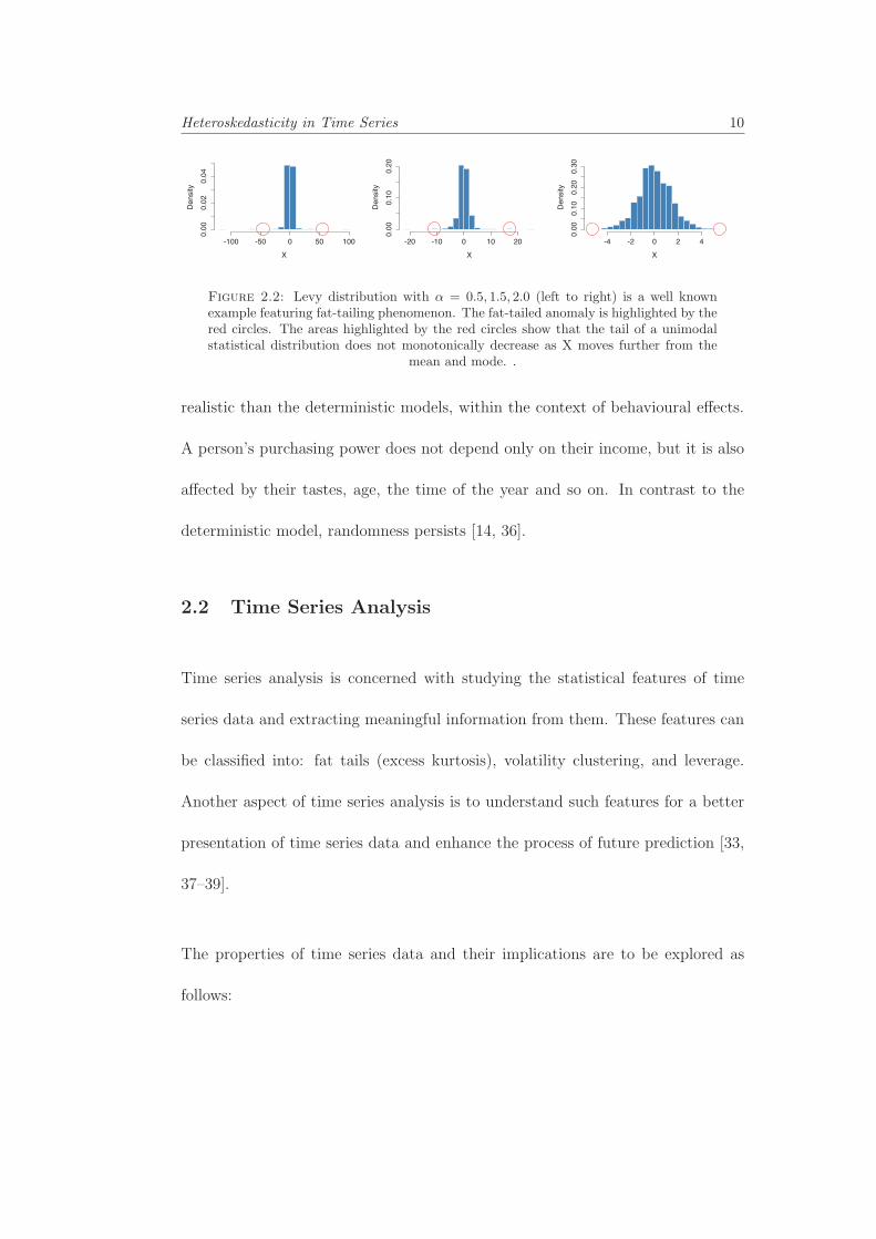
Figure 2.2: Levy distribution with α = 0.5, 1.5, 2.0 (left to right) is a well knownexample featuring fat-tailing phenomenon. The fat-tailed anomaly is highlighted by thered circles. The areas highlighted by the red circles show that the tail of a unimodalstatistical distribution does not monotonically decrease as X moves further from the
mean and mode. .
realistic than the deterministic models, within the context of behavioural effects.
A person’s purchasing power does not depend only on their income, but it is also
affected by their tastes, age, the time of the year and so on. In contrast to the
deterministic model, randomness persists [14, 36].
2.2 Time Series Analysis
Time series analysis is concerned with studying the statistical features of time
series data and extracting meaningful information from them. These features can
be classified into: fat tails (excess kurtosis), volatility clustering, and leverage.
Another aspect of time series analysis is to understand such features for a better
presentation of time series data and enhance the process of future prediction [33,
37–39].
The properties of time series data and their implications are to be explored as
follows:
Heteroskedasticity in Time Series 11
The fat-tail phenomenon, sometimes referred to in the literature as heavy-tailed
distribution, is a feature of some probability distributions in which excess kurtosis
is exhibited. Kurtosis is a measure of distribution of a real valued random vari-
able around the mean. In [40], Plott was the first to address the problem of excess
kurtosis and its implications on the experimental market. However, Plott did not
introduce an explanation of such phenomena. In [3], Harvey addressed the fat
tailed disturbances in implementing their time series models with ARCH distur-
bances. Harvey’s transition equation expanded the scope of the model to cover
disturbances with fat tails. This was considered a breakthrough in the research
field, because the traditional Gaussian ARCH models did not seem to capture this
phenomenon, especially in the financial data [41–44]. Figure 2.2 illustrates the
difference between the normal and heavy tailed distributions.
The variation from a time period to the succeeding one is referred to as volatility
clustering or persistence. Volatility clustering refers to the fact that changes tend
to follow each other in their magnitude in an uncorrelated yet serially dependent
way [14, 18, 45]. It is a property of most heteroskedastic time series processes
used in the fields of finance and economics. Volatility clustering, as a type of
heteroskedasticity, attempts to explain part of the causes of excess kurtosis in the
time series data. Excess kurtosis can be partially the consequence of abnormalities
in the return distributions in the financial assets that experience fat tails.
The final characteristic of time series is measuring the leverage effect. This effect
was best described in the financial applications. It describes the case when the
Heteroskedasticity in Time Series 12
observed returns on the assets being examined have a negative relationship with
the changes observed in the volatility. For certain assets, a negative relationship
was observed between volatility trends and the expected returns. In other words,
volatility tends to rise when the returns are lower than expected and vice versa.
Time series analysis can accomplish many goals. Some of which are descriptive
analysis, spectral analysis, explanative analysis, forecasting and control analysis.
2.2.1 Descriptive Analysis
Descriptive analysis explains the trends and patterns experienced by the time
series. This can be illustrated either by plotting or by applying more advanced
statistical techniques. The approach most commonly applied is to plot and analyse
these trends and patterns such as: overall trends of the time series, outliers, turning
points and finally, the cyclic patterns in the data series.
2.2.2 Spectral Analysis
This analysis describes how cyclic components can be accounted for variations in
time series data. This type of analysis is sometimes referred to as the frequency do-
main, where an estimate of a spectrum over a range of frequencies can be obtained
and periodic components can be separated out from a noisy environment.

Heteroskedasticity in Time Series 13
2.2.3 Explanative Analysis
Explanative analysis, also known as cross correlation, describes a mechanism that
can develop a dependent time series, and can be estimated, given one or more
variable time series. This type of analysis aims to describe the data generation
in an appropriate statistical model. These models can be either univariate or
multivariate. Therefore, this type of analysis can provide an explanation for the
variations in the series.
2.2.4 Forecasting
Forecasting refers to predicting the future behaviour of the time series based on
how it reacted in the past, within a specified confidence limit. The stochastic cor-
relation between one observation and the succeeding one is to be utilised to predict
the future values based on the past history and the behaviour of the observation
[46–50]. In this case, we can classify time series into two components: the de-
terministic component (the forecast) and the random component (the uncertainty
related to the forecast). This can be illustrated as follows:
Yt = f(t− 1, X) + εt (2.1)
where f(t− 1, X) is the function of the independent component at time t− 1 and
εt represents the disturbances in the mean of Yt.
Heteroskedasticity in Time Series 14
2.2.5 Intervention or Control Analysis
This technique can be applied to prevent a certain event affecting the time series
from happening, given that we are confident that this event has an impact upon
the time series. We can then define this event and ensure that it will not affect
the time series data being investigated. This can be referred to as ”What if?”
forecasting.
A time series model illustrates that observations close together in time will be
more related than observations further apart. In other words, values for a given
period will be expressed as being driven from past values rather than from future
values. In these cases, the data can be stabilised to normalise the variance by
applying the algorithmic transformation. We can also make the seasonal effects
additive, which will make the effect constant from one year to another. Finally,
we can make the data normally distributed, which will reduce the skewness in the
data to apply appropriate statistics.
A time series can be described as a sequence of correlated random observations.
This correlation is utilised to predict the future values baed on the historical se-
quence of the observed data under investigation. Statisticians have been spending
a lot of time and effort developing models that lead to better predictions based on
past data. They have been facing challenges of model limitations, errors and dif-
ferent natures of data that affect their calculations. The researchers in [48] offered
a comprehensive evaluation of forecasting techniques associated with volatility.
Heteroskedasticity in Time Series 15
2.2.6 ARMA-ARIMA Time Series Forecasting Techniques
One of the first efforts in the area of regression analysis is the Box-Jenkins ap-
proach [46]. Their development of the Autoregressive Integrative Moving Average
(ARIMA) model, which combined the Autoregressive (AR) and the moving aver-
age (MA) was a major breakthrough. This model is specialised in dealing with
the random shocks in the data at each corresponding time. Some assumptions
about these shocks are to be identified by the time series. These assumptions can
be described as follows: zero mean, constant variance, a normal distribution and
finally, no covariance detected between one shock and another. ARIMA (p,d,q)
model covers the following main aspects: Autoregression, Integration and Mov-
ing average. The autoregression [ARIMA(p,0,0)] describes the importance of the
preceding values of the series to the current ones over time. But the data val-
ues tend to decrease over time on an exponential basis. Consequently, this effect
will continue to decrease until it is nearly zero. It is represented by the following
equation
Yt = φ1Y(t−1) + αt (2.2)
where φ has a constraint of being between -1 and 1.
The integration process [ARIMA (0,d,0)] aims towards removing the trends and
drift of the data which results in transferring non-stationary data into stationary.

Heteroskedasticity in Time Series 16
It works by subtracting the first observation from the second observation and so
on.
The order of the process rarely exceeds one. Although many unit root tests have
been introduced in the last three decades, identifying the integration (d) still
depends on the graph representing the time series. If the data exhibit apparent
deviations from stationarity, it will not be appropriate to assign d value as zero.
Finally, there is the moving average process [ARIMA(0,0,q)]. This process is
concerned with the serially correlated data and which can be represented as
Yt = αt − θαt − 1 (2.3)
Generally, The ARIMA is fitted to the time series to perform one of two basic
time series models functions[51, 52]. It is either fitted to the data to provide us
with a better understanding of the data in hand, or to perform forecasting based
on the current data given.
To identify the most appropriate ARIMA model for a time series, we start by
differencing in order to make the series stationary and eliminate the gross feature
of seasonality. This is the first step in the Box-Jenkins approach that can be
referred to as the (de-trending of the series). One may transform a series by
taking the first differences as
Yt = ηt − ηt−1 = (1− β)ηt (2.4)
Heteroskedasticity in Time Series 17
There are many results to the differencing process. If the differenced series Yt
is an ARMA process, ηt is known as ARIMA process. But when Yt represents
iid random variables and ARMA is a (0,0) process, then ηt is an ARMA process.
Finally, when Yt process is a stationary ARMA (p,q) process, ηt is an ARIMA
(p,1,q)process or an ARMA (p+1,q) process with An AR unit root.
In practice, the differencing technique is not the only way to eliminate the trends
and seasonal effects. One may also eliminate the seasonality by other techniques
such as regression or by estimating a seasonal ARMA model.
The second step in the Box-Jenkins approach is identification. Identifying the
proper ARMA model has never been an easy task. For convenience, many pro-
grams today simply use the 95% confidence level. One might say that these bounds
are used mostly to identify and check the autocorrelations of the white noise. The
primary tools for dealing with autocorrelations are either the autocorrelations or
partial autocorrelations plots. The sample autocorrelation plots are compared to
the theoretical behaviour plots when the order is known. For a stationary and
invertible ARMA (p,q) model, both autocorrelation and partial autocorrelation
decay to zero and don’t have any unexpected cutoff points. Which is why in the
literature we consider the process of identifying the ARMA order both arbitrary
and difficult [34, 53].
The last step in the Box-Jenkins model is the model estimation. For ARMA
models, we have to estimate the order of the autoregressive process (p), and the
Heteroskedasticity in Time Series 18
moving average process (q). For the (p) process, the sample autocorrelation should
have an exponentially decreasing nature. However, it might combine a mixture of
both exponentially decreasing and sinusoidal components.
As for the estimation of the MA component of the ARMA model, it is more
involved because the innovations or white noise part εt are not observable and
only can be computed recursively. The autocorrelation function of MA becomes
zero at lag q+1 and greater. So, when we are examining the sample autocorrelation
function, we are mainly concerned with where the plot tends to be zero. This can
be done by presuming a confidence level of 95% for the sample autocorrelation
function on the sample autocorrelation plot.
We can sum up the Box-Jenkins model in the following points: The ARMA model
is designed to transform time series that are characterised with seasonal effects
and stochastic trends to non-stationary time series. It is mainly used to repre-
sent the transitory dependence. Estimation using the Box-Jenkins model is of
such complexity that most of the literature argues that it is preferable to leave
the process of parameter estimation to high quality software. [46]. This mainly
applies to the non-linear estimation, in which the non-linear last square approach
is recommended.
There are other non-linear models to represent the changes of variances in a time
series (Heteroskedasticity) [25, 54]. Examples include but are not limited to:
Heteroskedasticity in Time Series 19
ARCH, GARCH, E-GARCH and others. These models are concerned with study-
ing heteroskedasticity not as a problem to be corrected, but as a prediction to be
computed. In the field of econometrics, ARCH and GARCH models were proven
in the literature to cover lots of the aspects related to heteroskedasticity. They
perform in a much sophisticated yet comprehensive approach. This section aims
to provide a basic comparative study between two of the core models addressing
heteroskedasticity, ARCH and GARCH models. It aims to define the strengths
and weaknesses of each model, the statistical modelling behind each and finally the
researchers’ contributions in each model. This will explain why researchers prefer
one model to the other, and explains why they are still interested in understanding
the statistics behind each of them.
2.3 ARCH Model
Engle [19] was the first to introduce ARCH model. ARCH stands for Autoregres-
sive conditional heteroskedasticity. Autoregressive indicates a feedback mechanism
that incorporates past and present observations. While conditional means that the
variance relies basically on the immediate past. ARCH is based on the concept
that the unconditional variance is left constant while allowing the conditional vari-
ance to change. This change is applied over a period of time and is represented as a
function of past errors. This process is characterised by having a zero mean and se-
rially uncorrelated with non-constant variances, having these variances conditional
on the past error terms, but they have constant unconditional variances. ARCH
Heteroskedasticity in Time Series 20
model has proven success, especially in identifying and analysing major sophisti-
cated economic phenomena. In Engle [20] and Engle and Kraft [2], applications
on economic inflation were discussed. These models recognised the volatility of
inflation. With a known zero mean, the model can be represented as
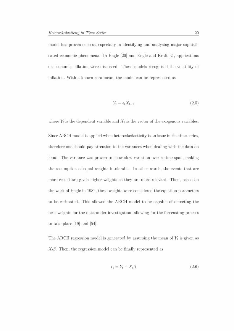
Yt = εtXt−1 (2.5)
where Yt is the dependent variable and Xt is the vector of the exogenous variables.
Since ARCH model is applied when heteroskedasticity is an issue in the time series,
therefore one should pay attention to the variances when dealing with the data on
hand. The variance was proven to show slow variation over a time span, making
the assumption of equal weights intolerable. In other words, the events that are
more recent are given higher weights as they are more relevant. Then, based on
the work of Engle in 1982, these weights were considered the equation parameters
to be estimated. This allowed the ARCH model to be capable of detecting the
best weights for the data under investigation, allowing for the forecasting process
to take place [19] and [54].
The ARCH regression model is generated by assuming the mean of Yt is given as
Xtβ. Then, the regression model can be finally represented as
εt = Yt −Xtβ (2.6)

Heteroskedasticity in Time Series 21
The ARCH regression model has a range of features, making it more plausible for:
1. Econometric applications: Econometric forecasters are capable of forecasting
and predicting the future variation in the data from one period to another. ARCH
emphasises on the fact that future forecast varies over time and rely on the past
errors in their prediction. 2. Monetary theory and theory of finance. The portfolios
of financial assets depend on their estimation on the rates of returns. Therefore,
the variations in the expected means and variances on such returns consequently
affect the prediction of such asset prices. ARCH has shown access in handling
the uncertainties of such equities by studying the nature of the variances within
the constrained regression model. 3. Forecasting is conditionally deterministic.
It does not leave any uncertainty in the process of expecting the squared error in
time t when compared to past error terms.
We can claim that the ARCH model analyses the effect of omitting the vari-
ables from the estimated model. ARCH literature made a major breakthrough in
predicting the volatility of economic time series, making it possible to analyse the
apparent changes in volatility, and identifying the impact of non-linear dependence
of the parameters in the economic model.
Applying ARCH models is a straight forward process. They handle the collective
errors, they take of non-linearities and finally, they adapt to the change in the per-
sonal capabilities of the economic forecaster. From the statistical point of view,
the ARCH models may be considered considered as some specific non-linear time
series models. This will allow for a quite exhausting studying of the underlying
Heteroskedasticity in Time Series 22
dynamics. On the other hand, the ARCH model failed to capture irregular phe-
nomena especially in the financial and econometric sector such as crashes, mergers,
news effects or threshold effects. We can claim that ARCH models are not offering
the flexibility required for capturing the persistence in volatility [22].
Finally, we can summarise the strategic features of ARCH models as follows:
1. ARCH models are playing a very important role in identifying the stochastic
nature of the error terms, for both linear and non-linear econometric models; and
2. ARCH models allow for the prediction of the average size of error terms when
fitted to empirical data.
Although ARCH modelling showed some great capabilities handling the stochastic
features and nature of time series data, there was an apparent need to generalise
this model to enhance its performance. This consequently led to the introduction
of the generalised ARCH model known as GARCH.
2.4 GARCH model
GARCH is considered a useful generalisation of ARCH modelling. Bollerslev first
introduced it in 1986 [55]. The GARCH model aims to help with the study of past
variances in order to explain future ones. GARCH model explains the dependence
of the time series model on volatility. Generalising Engle’s ARCH technique, the
GARCH model included both the autoregressive (AR) as well as moving average

Heteroskedasticity in Time Series 23
(MA) terms. It has the advantage of using fewer parameters. This will subse-
quently increase its computational efficiency.
GARCH follows the understanding that all past errors contribute to forecast
volatility. This is to be considered the most general case.The GARCH model
has proven success in the area of predicting conditional variance. GARCH was
able to capture the main features of the series under investigation by describing
the conditional variance. At the same time, it is simple enough to allow for much
investigative study of the available solutions.
The main application of GARCH, by definition, is when the series is heteroskedas-
tic; its variance is noticed of being changing over time. The error terms are
practically expected to change from one point to another. They might be large
for some points and small for others.
2.4.1 GARCH modelling
The GARCH model takes into consideration the fat-tail phenomena and volatility
clustering. There are the main basic features of time series data and the main
interest in studying time series analysis. The GARCH model has been widely
implemented in the field of finance. It was widely applied in fields including risk
management, portfolio management, option pricing, and foreign exchange. We can
apply the GARCH model to examine the relationship between long and short term
interest rates, analyse time varying risk premiums, and model foreign exchange
Heteroskedasticity in Time Series 24
markets that incorporates fat tail behaviour. GARCH effects can also be shown
in fields like capital allocation and value at risk (VaR) [23–25, 32, 54, 56–58].
GARCH’s model widely used specification is that the prediction of the variance in
the next period is dependent on weighted average of the long-run average variance.
This variance was statistically captured by the most recently observed squared
residuals. Many GARCH estimations are currently available through commercial
software such as MAtlab, SAS or TSP. These types of software offer a straight
forward process when using GARCH applications. First, we need to define the
parameters. These include ω, α and β. Second, start calculating an estimate of the
variance based on the first observation. Subsequently, it will be easy to identify the
estimate for the second observation. The GARCH updated formula will calibrate
the following parameters: a. A weighted average of the unconditional variance,
b. The squared residual of the first observation, and c. The starting variance
and estimates of the variances of the second observation. This formula will be the
input in estimating the third variance and a long time series variance forecast will
be constructed. A positive relationship was denoted between the residuals and the
time series constructed. A symmetric way to modify the parameters ω, α and β
to obtain the best fit by applying the likelihood function [26, 28, 59].
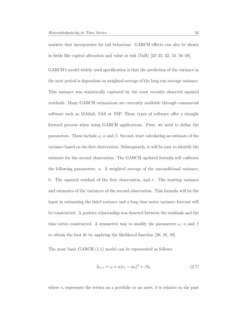
The most basic GARCH (1,1) model can be represented as follows:
ht+1 = ω + α(rt −mt)2 + βht (2.7)
where rt represents the return on a portfolio or an asset, h is relative to the past
Heteroskedasticity in Time Series 25
information set and ω,α and β are constants estimated by the econometricians
[54]. This only works if α + β < 1 and requiring that α > 0, β > 0 and finally
ω > 0.
Although the main application of the model is to forecast just one period, it
turned out that based on one period a two period forecast. Therefore, long-horizon
forecasts can be created. Referring to Engle again, in his work he claimed that
for GARCH (1,1) the unconditional variance can be addressed to represent the
distant-horizon forecast. This condition can be achieved if α + β < 1 for all the
time periods. This will ultimately imply that GARCH models are conditionally
heteroskedastic and the mean is driven yet the variance is unconditionally constant.
The GARCH (1,1) model can be expanded to the comprehensive GARCH (p,q)
model. This is a model where additional lag terms are provided. They are useful
when a long-term time series data is investigated. For example, several years of
data.
Heteroskedasticity of errors has disappeared with the adoption of more advanced
statistical data models. GARCH specification of error terms allowed for a more
accurate volatility forecast, and overcame the fact that most familiar statistical
models exhibit some sort of conditional error heteroskedasticity.
The GARCH success in predicting volatility changes allowed for a wide range
of applications in the fields of economics and finance. Risk management, option

Heteroskedasticity in Time Series 26
pricing, and asset allocations are some of the popular applications in finance. Their
effects are important in areas like efficient capital allocation and management.
The GARCH model has been intensively investigated by a wide range of re-
searchers. Their goal was to improve its performance and expand the areas of
its applications. The literature has identified some of the basic work and models
in the field. The basic model was developed by Bollerslev in [55], who then in-
troduced the I-GARCH model. Taylor in [60] introduced the TS-GARCH model.
Engle and Ng [61] suggested the NA-GARCH and the V-GARCH. The E-GARCH
and the NGARCH were introduced by Higgins in [27]. Hentshel in [62] introduced
the H-GARCH and the Aug-GARCH was suggested by Duan in [58]. The H-
GARCH and the Aug-GARCH specifications are very flexible and both models
include some of the features of the other previously stated GARCH models, mak-
ing them more reliable and mature.
In conclusion, we can clearly state that GARCH has proven accuracy in forecast-
ing and modelling time-varying conditional variances. It takes into consideration
basic time series features such as volatility clustering and excess kurtosis. GARCH
models led also to a fundamental change in the econometric approaches introduced
before. They have been considered important in the eyes of academics and practi-
tioners simply because their ease of use in practice and their richness in addressing
theoretical problems many of which have not been yet solved.

Heteroskedasticity in Time Series 27
2.4.2 Restrictions on GARCH model
There are some limitations avoiding the wide application of GARCH in finance.
GARCH functions in its finest capability under moderately stable market con-
ditions. GARCH fails to capture asymmetrical phenomena in most cases such
as unexpected events. These events can lead to substantial change. Finally, the
heteroskedasticity explains some, but not all ,fat tails behaviour in the financial
series.
One of the recent studies in the field [32] was dedicated to study the limitations of
GARCH model, particularly in detecting excess kurtosis and persistence in volatil-
ity. This was also related to the fact that GARCH model, especially in the financial
applications, does not give the required attention to the behavioural changes in
the market such as crashes and financial crisis. This research investigated the
impact of the simultaneous changes in the GARCH model parameters on the re-
turn series and its volatility. The results of this study found that GARCH model
parameters have an impact on both the volatility and the dynamic structure of
the series. The results of the study also concluded that one can get more informa-
tion by investigating the changes in individual model parameters rather than the
collective investigation of the parameters as one unit. This can be done assuming
that both the volatility and excess kurtosis change enduringly. These changes had
permanent effects on the volatility at all times, but only a change in parameters
α and β has that permanent impact on the excess volatility of the series.
Heteroskedasticity in Time Series 28
2.4.3 Outliers in GARCH model
Outliers can be defined as observations that are numerically distant from the data.
They are defined as “those that deviate from other members of the sample” [63].
They are often considered an error or noise, though they might carry essential
information. Therefore, we should pay proper attention to investigating outliers.
They contain valuable information about data collection and recording for the
process under investigation at many instances [64].
There are lots of reasons behind the appearance of outliers. This might be due
to human error, changes in the system behaviour, sample contamination with el-
ements from outside the population, or as a natural deviation in the population.
Also, outliers may appear by chance, error in data transmission or population
transcription or as an indication of measurement error or heavy-tailed distribu-
tions. One should be careful when dealing with outliers and not to conflict them
with experimental errors.
Outliers might include sample minimum or sample maximum or both, but sample
maximum or minimum are not always accordingly reported as outliers. Another
notable point about outliers is that in larger sampling of data, some data will be
noticed as far away from the sample mean than the reasonably accepted range.
This could be a consequence of incidental systematic error or flaw in the theory
generating the sample. In this case, outliers can designate faulty data, or an
application is where a specific theory might be considered invalid. It was also

Heteroskedasticity in Time Series 29
denoted that in large sampling, a small number of outliers will be detected.
Outliers can be classified into univariate and multivariate outliers. Univariate are
the outliers that are detected within a single variable either visually by examining
the data with a frequency distribution or by using a Box plot to identify the
extreme and mild outliers. While the multivariate outliers are those that occur
within the joint combination of two or more variables.
There are numerous problems associated with outliers detection. Determining
whether an observation is an outlier is highly subjective. The second problem is
that outliers mask each other. The estimated standard deviation is affected by the
size of the outlier. The estimated standard deviation shrinks when a large outlier
is removed. It gets worse by increasing the complexity of the data. The outliers
become visible when some others are removed.
GARCH model has been applied in the area of outliers detection. Based on the
work of [65], the GARCH (1,1) model was applied to detect and correct outliers
before estimating the risk measures in financial markets such as minimum capital
risk requirements. Their study has proven successful in generating more accurate
minimum capital risk requirements (MCCRs).
Heteroskedasticity in Time Series 30
2.5 Heteroskedasticity Challenges and Tests
The main assumption of the least square model is homoskedasticity. While het-
eroskedasticity is when the variances of the error terms of the data under investi-
gation are not equal. The error terms are expected to be larger from some point
to another. In this case, not only the deficiencies of the least square models are
corrected, but also a prediction is computed for the variance of each error term.
Causes of heteroskedasticity can include the following: 1. Model misspecification.
2. As the value of the independent variable increases, the errors may increase. 3.
As the values of the independent variable become more extreme in either directions,
errors increase. 4. Measurement errors can cause heteroskedasticity to appear in
the data being examined.
The consequences of heteroskedasticity of the data can be illustrated as follows:
1. Standard errors are biased when heteroskedasticity is present, which may lead
to biased test statistics and confidence interval. 2. In logistics regression, het-
eroskedasticity can produce biased and misleading parameter estimates.
In 1982, Engle presented two types of heteroskedasticity. The first type was when
the regression errors were heteroskedastic. This is because they rely in their com-
putation on the value of the independent variables. In this case, the average error
was positively related to the independent variable size.
Heteroskedasticity in Time Series 31
The second type represents the case in which the error terms vary with time
rather than the value of the process variables. Based on the literature in [59,
66], heteroskedasticity of error terms has not completely disappeared with the
acceptance of sophisticated financial and statistical model variables. There was no
evidence of a naturally developed process to model conditional heteroskedasticity.
Various attempts aim to identify different features of the data that seem relatively
important to the analysis. This relative importance and relevance of the data
makes it difficult to develop much more sophisticated and widely applicable model
that fits all the available data sets.
2.5.1 Heteroskedasticity Detection
Heteroskedasticity detection is representing an important issue when dealing with
Least squares estimation and linear regression models [67], particularly when het-
eroskedasticity is present in the error terms. This was proven to be influenced by
the sample size. In small samples, a valid test for heteroskedasticity represents a
challenge for analysts to obtain.
Visual detection of heteroskedasticity was first introduced by inspecting the resid-
uals plotted against the fitted values or by plotting the independent variable sus-
pected to be correlated with the variance of the error terms. If the residuals appear
to be roughly the same size for all values of X, or in small samples slightly larger
than the mean of X, then it is safe to assume that heteroskedasticity is not severe
enough to raise concern. On the other hand, if the plot shows uneven presentation
Heteroskedasticity in Time Series 32
of residuals, so that the width is larger for some values of X than for others, then
a heteroskedasticity test should be conducted.
Goldfeld and Quandt [68] have offered great contributions in tackling this prob-
lem. Their work was then modified by Phillips and Harvey in 1974 [67], based on
maintaining the residuals of the least square regression model. As for larger sam-
ples, Glejser [69], Park [70], and Rutemiller and Bowers [71] introduced a number
of tests to estimate certain forms of heteroskedasticity in larger sample sizes.
The starting point when studying heteroskedasticity was assuming the general
linear model
Y = (Xβ) + u (2.8)
where Y is an n*1 vector of observations on the dependent variable, X is an n ∗ k
matrix of observations on the K independent variables, and β is a K ∗ 1 vector
of regression coefficients, and finally u is an n ∗ 1 vector of stochastic disturbance
terms.
Based on the work first introduced by Harvey and Phillips in [67], heteroskedas-
ticity tests address two simple forms of heteroskedasticity
σ2j = σ2X2
ji (2.9)
and
Heteroskedasticity in Time Series 33
σ2j = σ2Xji (2.10)
We classify heteroskedasticity tests as follows:
2.5.2 The Goldfeld-Quandt test
The Goldefeld-Quandt test is categorised as a test for the discrete changes in
variances. In this test, the main assumption is that observations are in an as-
cending order based on increasing values of σ2j [68]. This test is concerned with
homoskedasticity in the regression analysis.It operates by comparing the variances
of error terms across discrete subgroups. Under homoskedasticity, all subgroups
should have the same estimated variances. The Goldfeld-Quandt test can be ex-
plained in the following equation:
ei = Y1 −X1b1 (2.11)
where b1 is a least squares estimate of β. It has a X2 distribution with
l − k = m (2.12)
where m represents the degrees of freedom under the null hypothesis.
This test offers a simple diagnosis for heteroskedastic errors in both univariate and
multivariate regression models, but it does not show robustness to specific types of
Heteroskedasticity in Time Series 34
errors. It cannot distinguish between heteroskedastic errors and the specification
problems as incorrect functional form. It was also noted that omitting central
observations may lead to a reduction in the degrees of freedom, which may lead
to inaccurate results of the test as well.
2.5.3 Ordinary likelihood ratio test
The ordinary likelihood ratio test can be represented as follows:
LT = −2{Lp(Y ; δ0)− L− p(Y ; δ)
}(2.13)
.
Rutemiller, Bowers and Harvey [71, 72] have derived this statistical test by apply-
ing specific weighting functions. Basically, their work was based on x2 distribution
with q degrees of freedom.
2.5.4 Conditional likelihood ratio test
First introduced by Honda [73] as a modification of Cox and Hinkley’s [74] work
in order to tackle the problems of applying the profile likelihood ratio test. The
results of this test can be summarised in failing to perform in small number of
noisy parameters. The conditional likelihood ratio test function can be illustrated
as following:
CLT = −2{CLp(Y ; δ0)− CLp(Y ; δ)
}(2.14)
.

Heteroskedasticity in Time Series 35
2.5.5 Modified likelihood ratio test
There is a lack of orthogonality between the parameter of interest δ and σ2, which
represents the nuisance parameter in the conditional likelihood ratio test. This
test was introduced by Simonoff and Tsai in 1994 [75] to solve these problems.
Their work was influenced by Cox and Reid’s work in 1987 [76].
In practical applications, orthogonal parameters are not that easy to handle or to
obtain. In 1993, Cox and Reid modified their model, in the form of an adjustment
for which explicit orthogonalization of the parameters is not required. In this case,
The resulting modified likelihood ratio test can be illustrated as follows:
ALT = CLT + 2(δ − δ0)Σni=1wi0/n (2.15)
.
evaluated at δ0 for i=1...,n
where
˙wi0 = ∂wi/∂δ (2.16)
The ALT was proven successful for the exponential weighting function, regardless
of whether or not the orthogonal parameter transformation is available.

Heteroskedasticity in Time Series 36
2.5.6 Residual likelihood ratio test
Verbyla 1993 [77] claimed that if the scale and the weighting parameters were
treated as the parameters of interest, the residual likelihood function is the same as
the conditional profile likelihood function, given the maximum likelihood estimates
of θ. The resulting function can be represented as follows:
RLp(Y ; σ2, δ) = RLp(Y |θ2σ; σ2, δ) = CLp(Y ; δ)− logσ2δ = MLp(Y ; δ)− logγδ
(2.17)
Given the fact that we are using the scale parameter as the parameter of interest,
the equation of the residual likelihood ratio test can be modified as follows:
RLT = CLT + 2(logσ20 − logσ2) (2.18)
We can take this equation one step further as following, when RLT is greater than
MLT:
RLT = MLT + 2(logγ0 − logγ). (2.19)
.
2.5.7 Breusch-Pagan Test
Breusch-Pagan test aims to detect for the conditional heteroskedasticity in a linear
regression model [78]. It tests for the continuous changes in variances. It measures
the dependency of the estimated variance of the residuals from the regression on
Heteroskedasticity in Time Series 37
the values of the independent variables. It tests the null hypothesis of all error
variances are all equal versus the alternative which is that error variances are a
multiplicative function of one or more variables. The bigger the predicted value
of y, the bigger the error variance. It is formulated as follows:
y = β0 + β1x+ u (2.20)
The estimated mean u, also known as the residual, is then estimated with a mean
equal to zero based on the ordinary least squares method (OLS).
u2 = β0 + β1x+ v (2.21)
.
The Breusch-Pagan test examines nR2 with K degree of freedom where n is the
number of observations, R is the regression of the squared residuals from the
original regression of the independent variables and k is the number of independent
variables. If the test shows that there is a joint significant dependency between the
dependent and the independent variables, then we can reject the null hypothesis
of homoskedasticity. When implementing the test, the examiner selects which
variables to include in the auxiliary equation as a judgment call. In this case, a
poor judgment can lead to poor test.
Heteroskedasticity in Time Series 38
The Breusch-Pagan test failed to work well for non-linear forms of heteroskedas-
ticity. For example, when the error variances get larger as x gets more extreme
in either directions. Also, it has problems when the error terms are not normally
distributed.
2.5.8 White Test
The White test, named after its founder Halbert White [79], is a direct test of
heteroskedasticity. It is a special case of Breusch-Pagan test. It solves the prob-
lems regarding the execution of the Breusch-Pagan and it is more general. It
adds a lot of terms to test for more types of heteroskedasticity. For example, by
adding the squares of regressors, it detects the non-linearities such as an hour-glass
shape. It operates by assuming that there is no prior knowledge of the existence
of heteroskedasticity in the sample being examined. This test can be illustrated
as follows:
Yt = β0 + β1Xt1 + β2Xt2 + ut (2.22)
σ2t = α0 + α1Xt1 + α2Xt2 + · · · (2.23)
The White test operates by accepting or rejecting the null hypothesis of the data
being of equal variances. If the null hypothesis is not rejected, we can say that the
residuals in the examined sample are homoskedastic. Alternatively, if we reject the
Heteroskedasticity in Time Series 39
null hypothesis, the residuals are recognised as heteroskedastic. In order to accept
or reject the homoskedasticity hypothesis, we need to calculate nR2 where n is
the size of the sample and the R is the unadjusted R-squared from the auxiliary
regression of μt as the dependent variable against the constants Xt1, Xt2.
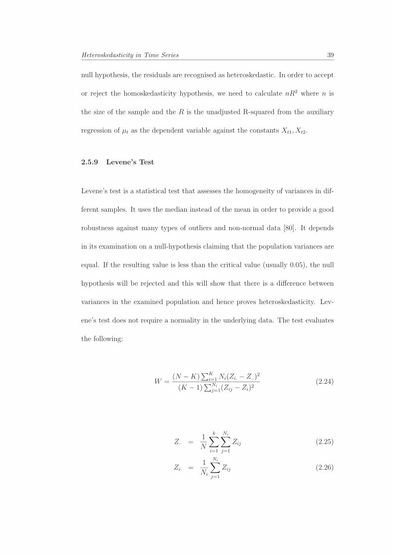
2.5.9 Levene’s Test
Levene’s test is a statistical test that assesses the homogeneity of variances in dif-
ferent samples. It uses the median instead of the mean in order to provide a good
robustness against many types of outliers and non-normal data [80]. It depends
in its examination on a null-hypothesis claiming that the population variances are
equal. If the resulting value is less than the critical value (usually 0.05), the null
hypothesis will be rejected and this will show that there is a difference between
variances in the examined population and hence proves heteroskedasticity. Lev-
ene’s test does not require a normality in the underlying data. The test evaluates
the following:
W =(N −K)
∑Ki=1 Ni(Zi. − Z..)
2
(K − 1)∑Ni
j=1(Zij − Zi)2(2.24)
Z·· =1
N
k∑i=1
Ni∑j=1
Zij (2.25)
Zi· =1
Ni
Ni∑j=1
Zij (2.26)
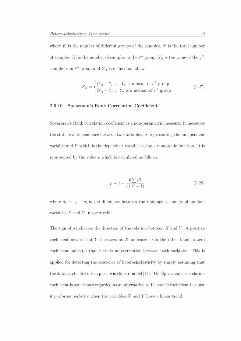
Heteroskedasticity in Time Series 40
where K is the number of different groups of the samples, N is the total number
of samples, Ni is the number of samples in the ith group, Yij is the value of the jth
sample from ith group and Zij is defined as follows:
Zij =
{|Yij − Yi·|, Yi· is a mean of ith group
|Yij − Yi·|, Yi· is a median of ith group(2.27)
2.5.10 Spearman’s Rank Correlation Coefficient
Spearman’s Rank correlation coefficient is a non-parametric measure. It measures
the statistical dependence between two variables, X representing the independent
variable and Y which is the dependent variable, using a monotonic function. It is
represented by the value ρ which is calculated as follows:
ρ = 1− 6∑
d2in(n2 − 1)
(2.28)
where di = xi − yi is the difference between the rankings xi and yi of random
variables X and Y , respectively.
The sign of ρ indicates the direction of the relation between X and Y . A positive
coefficient means that Y increases as X increases. On the other hand, a zero
coefficient indicates that there is no correlation between both variables. This is
applied for detecting the existence of heteroskedasticity by simply assuming that
the data can be fitted to a piece-wise linear model [48]. The Spearman’s correlation
coefficient is sometimes regarded as an alternative to Pearson’s coefficient because
it performs perfectly when the variables X and Y have a linear trend.

Heteroskedasticity in Time Series 41
2.5.11 Heteroskedasticity challenges
This section will address the most common ways that have been utilised for the
past periods when dealing with heteroskedasticity. It will be illustrated as follows:
1. Respecify the model or transform the variable: Sometimes, some important
variables are left out of the model. If the reason for heteroskedasticity was found
to be the misspecification of the model, then by checking for heteroskedasticity we
might be able to identify the model specification problems.
2. Use robust standard errors: when heteroskedasticity exists, robust standard
errors tend to be more trustworthy. It addresses the problem of errors that are
not independent and identically distributed. It will not change the coefficient
estimates provided by the Ordinary Least Squares (OLS), but it will change the
standard errors and significance tests results. As for outliers, we can use robust
regression by using a weighing scheme that causes outliers to have less impact on
the estimates of regression coefficients. In this case, robust regression will produce
different coefficient estimates than the ordinary least squares.
3. Use weighted least squares: generalised least squares is a technique that will
always result in estimators that are Best Linear Unbiased Estimator (BLUE) when
either heteroskedasticity or serial correlations are present. Ordinary Least Squares
works by selecting coefficients that minimise the sum of squared regression resid-
uals
∑(Yj − Yj)
2 (2.29)
Heteroskedasticity in Time Series 42
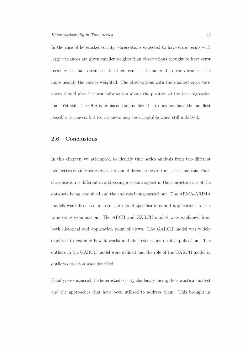
In the case of heteroskedasticity, observations expected to have error terms with
large variances are given smaller weights than observations thought to have error
terms with small variances. In other terms, the smaller the error variances, the
more heavily the case is weighted. The observations with the smallest error vari-
ances should give the best information about the position of the true regression
line. Yet still, the OLS is unbiased but inefficient. It does not have the smallest
possible variances, but its variances may be acceptable when still unbiased.
2.6 Conclusions
In this chapter, we attempted to identify time series analysis from two different
perspectives: time series data sets and different types of time series analysis. Each
classification is different in addressing a certain aspect in the characteristics of the
data sets being examined and the analysis being carried out. The ARMA-ARIMA
models were discussed in terms of model specifications and applications to the
time series examination. The ARCH and GARCH models were explained from
both historical and application point of views. The GARCH model was widely
explored to examine how it works and the restrictions on its application. The
outliers in the GARCH model were defined and the role of the GARCH model in
outliers detection was identified.
Finally, we discussed the heteroskedasticity challenges facing the statistical analyst
and the approaches that have been utilised to address them. This brought us

Heteroskedasticity in Time Series 43
to the conclusion that a new model or approach can be introduced to face the
heteroskedasticity challenges and enable for a more reliable outcome.

Chapter 3
Critical Review of the Literature
ARCH and GARCH models are playing important roles in the analysis of time
series data. The importance of the ARCH and GARCH models is highlighted
when the study aims to analyze and forecast volatility, particularly in the financial
applications.
This section aims to provide a basic comparative study between two of the core
models addressing heteroskedasticity, the ARCH and GARCH models. It aims
to define the strengths and weaknesses of each model, the statistical modelling
behind each and finally the researchers’ contributions in each model. This will
explain why researchers prefer one model to the other, and explains why the they
are still interested in understanding the statistics behind each of them.
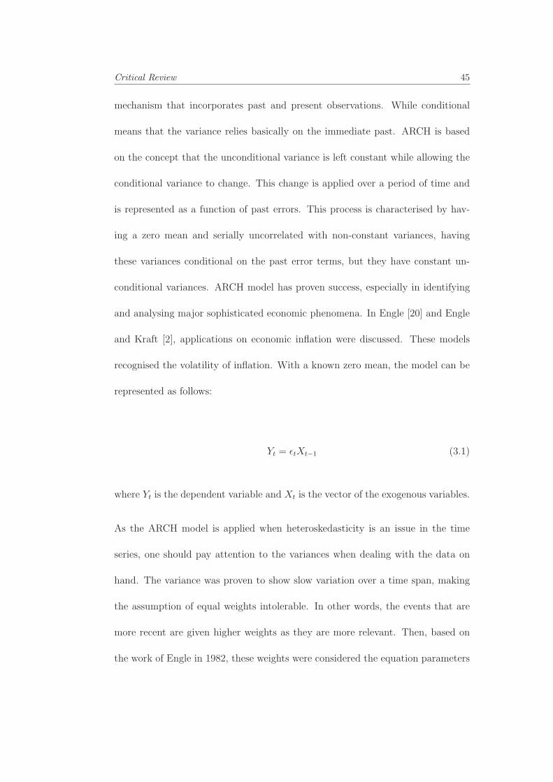
3.1 ARCH model
Engle [19] was the first to introduce the ARCH model. ARCH stands for Au-
toregressive conditional heteroskedasticity. Autoregressive indicates a feedback
44
Critical Review 45
mechanism that incorporates past and present observations. While conditional
means that the variance relies basically on the immediate past. ARCH is based
on the concept that the unconditional variance is left constant while allowing the
conditional variance to change. This change is applied over a period of time and
is represented as a function of past errors. This process is characterised by hav-
ing a zero mean and serially uncorrelated with non-constant variances, having
these variances conditional on the past error terms, but they have constant un-
conditional variances. ARCH model has proven success, especially in identifying
and analysing major sophisticated economic phenomena. In Engle [20] and Engle
and Kraft [2], applications on economic inflation were discussed. These models
recognised the volatility of inflation. With a known zero mean, the model can be
represented as follows:
Yt = εtXt−1 (3.1)
where Yt is the dependent variable and Xt is the vector of the exogenous variables.
As the ARCH model is applied when heteroskedasticity is an issue in the time
series, one should pay attention to the variances when dealing with the data on
hand. The variance was proven to show slow variation over a time span, making
the assumption of equal weights intolerable. In other words, the events that are
more recent are given higher weights as they are more relevant. Then, based on
the work of Engle in 1982, these weights were considered the equation parameters
Critical Review 46
to be estimated. This allowed the ARCH model to be capable of detecting the
best weights for the data under investigation, allowing for the forecasting process
to take place [19] and [54].
The ARCH regression model is generated by assuming the mean of Yt is given as
Xtβ. Then, the regression model can be finally represented as follows:
εt = Yt −Xtβ (3.2)
The ARCH regression model has a range of features, making it more plausible
for: 1. Econometric applications: Econometric forecasters are capable of forecast-
ing and predicting the future variation in the data from one period to another.
ARCH emphasises on the fact that future forecast varies over time and rely on the
past errors in their prediction. 2. Monetary theory and theory of finance. The
portfolios of financial assets depend on their estimation on the rates of returns.
The variations in the expected means and variances on such returns consequently
affect the prediction of such asset prices. ARCH has shown access in handling
the uncertainties of such equities by studying the nature of the variances within
the constrained regression model. 3. Forecasting is conditionally deterministic.
It does not leave any uncertainty in the process of expecting the squared error in
time t when compared to past error terms.
We can claim that the ARCH model analyses the effect of omitting the vari-
ables from the estimated model. ARCH literature made a major breakthrough in
predicting the volatility of economic time series, making it possible to analyse the

Critical Review 47
apparent changes in volatility, and identifying the impact of non-linear dependence
of the parameters in the economic model.
Applying ARCH models is a straight forward process. They handle the collective
errors. They take of non-linearities and finally, they adapt to the change in the
personal capabilities of the economic forecaster. From the statistical point of
view, the ARCH models may be considered as some specific non-linear time series
models. This will allow for a quite exhausting studying of the underlying dynamics.
On the other hand, ARCH model failed to capture irregular phenomena especially
in the financial and econometric sector such as crashes, mergers, news effects or
threshold effects. We can claim that ARCH models are not offering the flexibility
required for capturing the persistence in volatility [22].
Finally, we can summarise the strategic features of ARCH models as follows:
1. ARCH models are playing a very important role in identifying the stochastic
nature of the error terms, for both linear and non-linear econometric models.
2. ARCH models allow for the prediction of the average size of error terms when
fitted to empirical data.
Although ARCH model showed some great capabilities handling the stochastic
features and nature of time series data, there was a great need to generalise this
model to enhance its performance. This consequently led to the introduction of
the generalised ARCH model known as GARCH.
Critical Review 48
3.2 GARCH model
GARCH is considered a useful generalisation of ARCH model. It was first in-
troduced by Bollerslev in 1986 [55]. GARCH model aims to help with the study
of past variances in order to explain future ones. GARCH model explains the
dependence of the time series model on volatility. Generalising Engle’s ARCH
technique, GARCH model included both the autoregressive (AR) as well as mov-
ing average (MA) terms. It has the advantage of using fewer parameters. This
will subsequently increase its computational efficiency.
GARCH follows the understanding that all past errors contribute to forecast
volatility. This is to be considered the most general case. GARCH model has
proven success in the area of predicting conditional variance. GARCH was able
to capture the main features of the series under investigation by describing the
conditional variance. At the same time, it is simple enough to allow for a much
investigative study of the available solutions.
The main application of AGRCH by definition is when the series is heteroskedastic;
its variance is noticed of being changing over time. The error terms are practically
expected to change from one point to another. They might be large for some
points and small for others.
Critical Review 49
3.2.1 GARCH modelling
GARCH model takes into consideration the fat tail phenomena and volatility clus-
tering. There are the main basic features of time series data and the main interest
in studying time series analysis. GARCH model has been widely implemented in
the field of finance. It was widely applied in fields like risk management, portfolio
management, option pricing, and foreign exchange. We can apply GARCH model
to examine the relationship between long and short term interest rates, analyse
time varying risk premiums, and model foreign exchange markets that incorpo-
rates fat tail behaviour. GARCH effects can also be shown in fields like capital
allocation and value at risk (VaR).
GARCH model widely used specification is that the prediction of the variance in
the next period is dependent on weighted average of the long-run average variance.
This variance was statistically captured by the most recently observed squared
residuals. Many of the GARCH estimations are currently available through com-
mercial software such as Matlab, SAS or TSP. These types of software offer a
straight forward process when applying GARCH applications. First, we need to
define the parameters. These include ω, α and β. Second, start calculating an
estimate of the variance based on the first observation. Subsequently, it will be
easy to identify the estimate for the second observation. The GARCH updated
formula will calibrate the following parameters: a. A weighted average of the
unconditional variance, b. The squared residual of the first observation, and c.
The starting variance and estimates of the variances of the second observation.
Critical Review 50
This formula will be the input in estimating the third variance and a long time
series variance forecast will be constructed. A positive relationship was denoted
between the residuals and the time series constructed. A symmetric way to mod-
ify the parameters ω, α and β to obtain the best fit by applying the likelihood
function[56].
The most basic GARCH (1,1) model can be represented as follows:
ht+1 = ω + α(rt −mt)2 + βht (3.3)
where rt represents the return on a portfolio or an asset, h is relative to the past
information set and ω,α and β are constants estimated by the econometricians
[54]. This only works if α + β < 1 and requiring that α > 0, β > 0 and finally
ω > 0.
Although the main application of the model is to forecast just one period, it
turned out that based on one period, a two period forecast can be developed.
Therefore, long-horizon forecasts can be created. Referring to Engle again, in
his work he claimed that for GARCH (1,1) the unconditional variance can be
addressed to represent the distant-horizon forecast. This condition can be achieved
if α + β < 1 for all the time periods. This will ultimately imply that GARCH
models are conditionally heteroskedastic and the mean is driven yet the variance
is unconditionally constant.
The GARCH (1,1) model can be expanded to the comprehensive GARCH (p,q)

Critical Review 51
model. This is a model where additional lag terms are provided. They are useful
when a long-term time series data is investigated. For example, several years of
data.
Heteroskedasticity of errors has disappeared with the adoption of more advanced
statistical data models. GARCH specification of error terms allowed for a more
accurate volatility forecast, and overcame the fact that most familiar statistical
models exhibit some sort of conditional error heteroskedasticity.
The GARCH success in predicting volatility changes allowed for a wide range
of applications in the fields of economics and finance. Risk management, option
pricing, and asset allocations are some of the popular applications in finance. Their
effects are important in areas like efficient capital allocation and management.
The GARCH model has been intensively investigated by a wide range of re-
searchers. Their goal was to improve its performance and expand the areas of
its applications. The literature has identified some of the basic work and models
in the field. The basic model was developed by Bollerslev in [55], who then in-
troduced the I-GARCH model. Taylor in [60] introduced the TS-GARCH model.
Engle and Ng [61] suggested the NA-GARCH and the V-GARCH. The E-GARCH
and the NGARCH were introduced by Higgins in [27]. Hentshel in [62] introduced
the H-GARCH and the Aug-GARCH was suggested by Duan in [58]. The H-
GARCH and the Aug-GARCH specifications are very flexible and both models
include some of the features of the other previously stated GARCH models, mak-
ing them more reliable and mature.
Critical Review 52
In conclusion, we can clearly state that GARCH has proven accuracy in forecast-
ing and modelling time-varying conditional variances. It takes into considerations
basic time series features such as volatility clustering and excess kurtosis. GARCH
models led also to a fundamental change in the econometric approaches introduced
before. They have been considered important in the eyes of academics and practi-
tioners simply because their ease of use in practice and their richness in theoretical
problems many of which has not been yet solved.
3.2.2 Restrictions on GARCH model
There are some limitations avoiding the wide application of GARCH in finance.
GARCH functions in its finest capability under moderately stable market con-
ditions. GARCH fails to capture asymmetrical phenomena in most cases such
as unexpected events. These events can lead to substantial change. Finally, the
heteroskedasticity explains some but not all of fat tails behaviour in the financial
series.
One of the recent studies in the field [32] was dedicated to study the limitations
of GARCH model, particularly in detecting excess kurtosis and persistence in
volatility. This was also related to the fact that GARCH model, especially in
the financial applications, does not give the required attention to the behavioural
changes in the market such as crashes and financial crisis. They investigated
the impact of the simultaneous changes in the GARCH model parameters on the
return series and its volatility. They found that they have an impact on both

Critical Review 53
the volatility and the dynamic structure of the series. They also concluded that
one can get more information by investigating the changes in individual model
parameters rather than the collective investigation of the parameters as one unit.
This can be done assuming that both the volatility and excess kurtosis change
enduringly. These changes had permanent effects on the volatility at all times,
but only a change in parameters α and β has that permanent impact on the
excess volatility of the series.
3.2.3 Outliers in GARCH modeling
Outliers can be defined as observations that are numerically distant from the data.
They are defined as “Those that deviate from other members of the sample” [63].
They are often considered an error or noise, though they might carry essential
information. Therefore, we should pay proper attention to investigating outliers.
They contain valuable information about data collection and recording for the
process under investigation at many instances [50, 64].
There are lots of reasons behind the appearance of outliers. This might be due
to human error, changes in the system behaviour, sample contamination with el-
ements from outside the population, or as a natural deviation in the population.
Also, outliers may appear by chance, error in data transmission or population
transcription or as an indication of measurement error or heavy-tailed distribu-
tions. One should be careful when dealing with outliers and not to conflict them
with experimental errors.
Critical Review 54
Outliers might include sample minimum or sample maximum or both, but sample
maximum or minimum are not always accordingly reported as outliers. Another
remark about outliers is that in larger sampling of data, some data will be noticed
as far away from the sample mean than the reasonably accepted range. This could
be a consequence of incidental systematic error or flaw in the theory generating
the sample. In this case, outliers can designate faulty data, or an application is
where a specific theory might be considered invalid. It was also denoted that in
large sampling, a small number of outliers will be detected [65].
Outliers can be classified into univariate and multivariate outliers. Univariate are
the outliers that are detected within a single variable either visually by examining
the data with a frequency distribution or by using a Box plot to identify the
extreme and mild outliers. While the multivariate outliers are those that occur
within the joint combination of two or more variables.
There are lots of problems associated with outliers detection. Defining whether an
observation is an outlier is very subjective. The second problem is that outliers
mask each other. The estimated standard deviation is affected by the size of the
outlier. The estimated standard deviation shrinks when a large outlier is removed.
It gets worse by increasing the complexity of the data. The outliers become visible
when some others are removed.
The GARCH model has been applied in the area of outliers detection. Based on
the work of [65], the GARCH (1,1) modelling was applied to detect and correct
outliers before estimating the risk measures in financial markets such as minimum
Critical Review 55
capital risk requirements. Their study has proven successful in generating more
accurate minimum capital risk requirements (MCCRs).
3.3 Prediction Interval Modelling
Statistically speaking, a prediction interval is defined as an estimate interval in
which the future observations will fall, within a certain probability. It depends
in its mechanism on the already observed data, or what we call the past observa-
tions. It predicts the distribution of the individual future points rather than the
true population mean or other quantities that can not be observed in this matter.
These later information can be detected and analysed by applying confidence in-
tervals. Confidence intervals take into consideration the unobservable population
parameters [22].
Many recent papers utilise prediction intervals to forecast the future values of
time series under examination. In [52], Pellegrini has been studying the impact
of heteroskedastic time series with stochastic trends on the prediction intervals.
They applied their study on a conditionally heteroskedastic model with a level of
stochasticity. In their research, they applied ARIMA-GARCH model to generate
the prediction intervals. They claimed that the lengths of the prediction intervals
will vary depending on whether the conditional heteroskedasticity affects the long-
run or short-run component.
However, their study was based on a moderate sample size. It showed that if the
source of heteroskedasticity was well explained, the uncertainty of the parameter
Critical Review 56
estimation will not have an influence on the construction of prediction intervals.
Yet, they did not succeed in establishing a mechanism to identify how to eliminate
the impact of heteroskedasticity when establishing prediction intervals for large-
sized financial data.
The problems associated with prediction intervals and their impacts have been
addressed by Baillie and Bollerslev in [81]. Their research focused on defining a
prediction for the variance in GARCH (p,q) model. Their work resulted in an
assumption of that by increasing the forecast horizon, the available information
become less significant and the optimal forecast converts to the unconditional
variance. With respect to the integrated GARCH (1,1) or IGARCH(1,1) models,
having α1+β1=1, the present piece of information becomes more relevant and
important for building up forecasts.
There were attempts to construct prediction intervals in [52]. Their study was
based on the ARIMA models for constructing a prediction interval. Their results
showed that due to the presence of unit root in this model, the prediction intervals
based on the ARIMA model always depend on excess volatility. Whether the
excess volatility is positive or negative determines if the prediction interval created
is either wide or narrow when compared to intervals built up by other competing
models. In that particular study, the opposing was the unobserved component
model. Neural network was also a key player in constructing prediction intervals.
In [82–85], leading techniques such as the Bayesian, the delta, the bootstrap models
were reviewed in terms of their contribution in constructing a prediction model for

Critical Review 57
future forecasting. Problems of uncertainties were also discussed and accounted
for to build the optimal neural-network based framework.
3.4 Conclusions
The ARCH regression model is an approximation to a more complex regression
which has non-ARCH disturbances. The ARCH specification might be by picking
up the effect of variables omitted from the estimated model.
A major contribution of the ARCH literature is the finding that apparent changes
in the volatility of economic time series may be predictable and result from a
specific type of non-linear dependence rather than exogenous structural changes
in variables. ARCH models are simple and easy to handle.They take care of
clustered errors, take care of non-linearities and can also take care of changes in
the econometrician’s ability to apply the forecasting models and techniques.
On the other hand, there are limitations and assumptions on the underlying ARCH
models. ARCH models assume a rather stable environment and fails to capture
irregular phenomena such as crashes, mergers , news effects or threshold effects
when studying irregularities such as financial markets applications.[60]
GARCH model is used in time series that exhibit time-varying volatility periods
of swings followed by periods of relative calm.
A wider exploration for ARCH and GARCHmodels was introduced in this chapter.
A historical and critical investigation of both ARCH and GARCH model was

Critical Review 58
implemented. The mechanism in which both ARCH and GARCH models operate
was illustrated, with the restrictions of the GARCH model being discussed.
Outliers detection and its impact on GARCH modelling was explained. The
GARCH model addresses the problem of heteroskedasticity and volatility clus-
tering of the time series by solving the outliers in the data and errors in the
outcome [21].
Chapter 4
SoLVI: Slope of Local VarianceIndex
Heteroskedasticity, by definition, is the phenomenon of having time varying vari-
ance in a time series [19, 55, 67]. As discussed in Chapter 2, measuring het-
eroskedasticity relies on estimating the change in variance relative to time. In
order to do that, a function should be derived to estimate local variance at a
certain time t within the time series y(t). This chapter starts with deriving equa-
tions for local estimation of mean μy(t) and variance σ2y(t) statistical parameters
of a time series y(t). Then two heteroskedasticity quantifying methods will be
presented. The first method is called heteroskedasticity variance index (HVI) re-
lies on estimating variance of local variances [35]. The second method, Slope of
Local Variance Index (SoLVI), evaluates the change in first derivative of the local
variance function ddtσ2y(t) [35].
59
SoLVI: Slope of Local Variance Index 60
4.1 Local Estimation of Statistical Parameters
Local estimation of statistical parameters is a well known technique in image
and signal processing [86–88]. The estimation is obtained by moving a kernel
window W of size N samples on the values of the time series y(t) and perform the
estimation procedure. The most common locally estimated statistical parameters
are mean μy(t) and variance σ2y(t).
4.1.1 Estimation of Local Average
Calculating local average is fairly simple. Let y(t) be the time series and μNy (t)
be the average of first N samples of y(t) at time t. The local average at time t is
then defined as
μNy (t) =
1
N
N∑i=t
y(i) (4.1)
This step is then repeated at subsequent samples yt+1, yt+2, ...yM , where M is the
total number of samples. In order to simplify and generalise the local calculation
procedure, signal processing convolution operator can be employed here. The
convolution operator ∗ : RM × RN → R
M+N−1 takes a time series yt as an input
and an N sized kernel h and is formulated as
(y ∗ h) (t) =∞∑
i=−∞y(t− i) · h(i) (4.2)
SoLVI: Slope of Local Variance Index 61
This formulation allows mathematicians to model different local operations on a
time series by simply changing the kernel h. The equations can then be further
simplified by using matrices mathematical structures by modelling y(t)|t=0..∞ as an
infinite vector yt = [y0, y1, ..., y∞], a time limited time series y(t)|t=0..M as a finite
vector yt = [y0, y1, ..., yM ] and an N sized kernel hNt = [h0, h1, ..., hN ]. Equation 4.2
can then be rewritten as
(y ∗ h) (t) =M−1∑i=0
y(t− i) · h(i) (4.3)
According to the formulation in eq. 4.3, an N sized averaging kernel is then for-
mulated as a 1×N vector
hNμ =
[1
N,1
N,1
N,1
N,1
N...,
1
N
](4.4)
or simply
hNμ =
1
N[1, 1, 1, 1, 1..., 1] (4.5)
Finally, the local average estimation equation can be summarised as
μNy (t) =
(y ∗ hN
μ
)(t) (4.6)
where hNμ = 1
N[1, 1, 1, 1, 1..., 1] is the N sized averaging kernel.
SoLVI: Slope of Local Variance Index 62
4.1.2 Generalisation with Gaussian Filters
In order to generalise the averaging kernel, a Gaussian formulation was used. Gaus-
sian generalisation replaces the averaging kernel hNμ with a zero mean Gaussian
kernel as follows:
gN,σμ (t) =
1
σ√2π
et2
2σ2 (4.7)
where gN,σμ is an averaging kernel with a standard deviation σ that gives more
weight to the sample yN2
and less weight to samples where yN2±i|i={1,..., 1
N} and
accordingly hNμ = gN,∞
μ .
4.1.3 Estimation of Local Variance
Locally estimated variance of a time series y(t) is a signal processing technique that
derives a time-based function of local variances σ2(t). It estimates the variance at
every spatial sample. The local variance signal is calculated using the expected
value notation V ar(X) = E(X2) − E(X)2. The expected value is calculated via
convoluting the y(t) with a moving average filter hN . Let hw be a 1×N average
linear shift invariant filter, the local average is then calculated as follows:
μNy (t) = hN(t) ∗ y(t) (4.8)
μNy2(t) = hN(t) ∗ [y(t)]2 (4.9)

SoLVI: Slope of Local Variance Index 63
where y(t)2 = y(t) · y(t) is calculated using the matrix Hadamard product. The
local variance function σ2y(t|w) is then calculated as follows:
σ2N
y (t) = μNy2(t)−
[μNy (t)
]2(4.10)
where[μNy (t)
]2= μN
y (t) · μNy (t) is calculated using the matrix Hadamard product.
In order to generalise the equations, the classic average filter hw can be replaced
by a Gaussian filter gNσ where σ controls the width of the Gaussian bell shape
and adjusts the weights for every spatial sample. The generalised local variance
function σ2N
y (t) with an averaging window is then defined as follows:
σ2N
y (t) = gNσ (t) ∗ y(t)2 − [gNσ (t) ∗ y(t)]2 (4.11)
Figure 4.1 illustrates local variance function overlaid on a homoskedastic (top) and
heteroskedastic (bottom) time series.
4.1.4 ARMA Filter
Selecting the proper size N of the convolution kernel is challenging. It relies on
the data size, the variability of data and the variance σ2 of Gaussian distribution
used in preparing the weighted average filter gNσ . On one hand minimising the
kernel size moves the assessment of the local variances towards simple time series
sampling and derives a zero-valued local variance as demonstrated in Figure 4.2.
On the other hand, maximising N yields a smoother local mean and variance
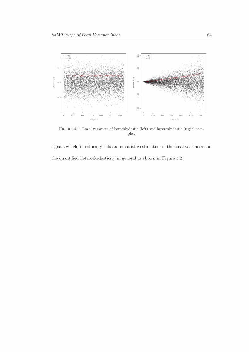
SoLVI: Slope of Local Variance Index 64
0 2000 4000 6000 8000 10000 12000
-20
2
samples t
y(t)an
dσy(t)
y(t)σy(t)
0 2000 4000 6000 8000 10000 12000
-200
-100
010
020
0
samples t
y(t)an
dσy(t)
y(t)σy(t)
Figure 4.1: Local variances of homoskedastic (left) and heteroskedastic (right) sam-ples.
signals which, in return, yields an unrealistic estimation of the local variances and
the quantified heteroskedasticity in general as shown in Figure 4.2.
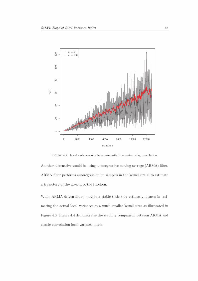
SoLVI: Slope of Local Variance Index 65
0 2000 4000 6000 8000 10000 12000
020
4060
8010
012
0
samples t
σy(t)
w = 5w = 100
Figure 4.2: Local variances of a heteroskedastic time series using convolution.
Another alternative would be using autoregressive moving average (ARMA) filter.
ARMA filter performs autoregression on samples in the kernel size w to estimate
a trajectory of the growth of the function.
While ARMA driven filters provide a stable trajectory estimate, it lacks in esti-
mating the actual local variances at a much smaller kernel sizes as illustrated in
Figure 4.3. Figure 4.4 demonstrates the stability comparison between ARMA and
classic convolution local variance filters.
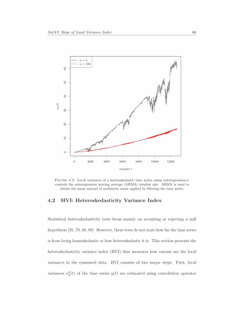
SoLVI: Slope of Local Variance Index 66
0 2000 4000 6000 8000 10000 12000
010
20
30
4050
60
samples t
σy(t)
w = 5w = 100
Figure 4.3: Local variances of a heteroskedastic time series using autoregression.wcontrols the autoregression moving average (ARMA) window size. ARMA is used to
obtain the mean instead of arithmetic mean applied by filtering the time series.
4.2 HVI: Heteroskedasticity Variance Index
Statistical heteroskedasticity tests focus mainly on accepting or rejecting a null
hypothesis [35, 79, 80, 89]. However, these tests do not state how far the time series
is from being homoskedastic or how heteroskedastic it is. This section presents the
heteroskedasticity variance index (HVI) that measures how variant are the local
variances in the examined data. HVI consists of two major steps. First, local
variances σ2y(t) of the time series y(t) are estimated using convolution operator
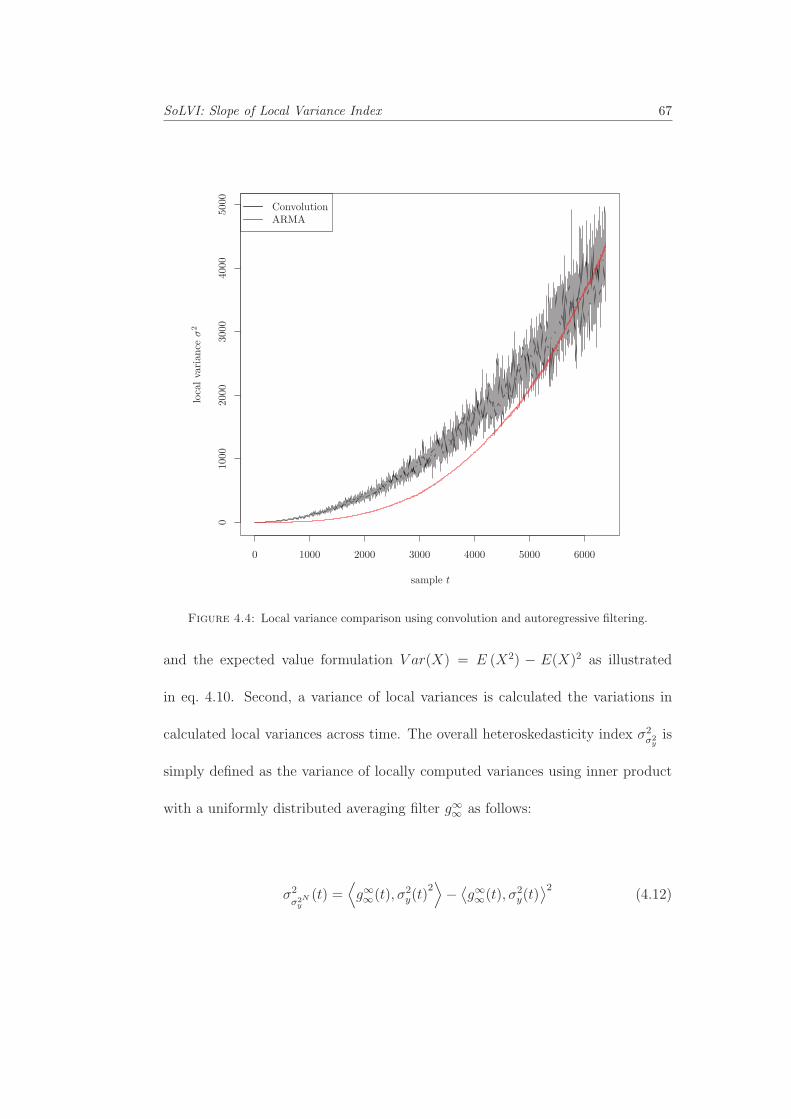
SoLVI: Slope of Local Variance Index 67
0 1000 2000 3000 4000 5000 6000
010
0020
0030
0040
0050
00
sample t
localvariance
σ2
ConvolutionARMA
Figure 4.4: Local variance comparison using convolution and autoregressive filtering.
and the expected value formulation V ar(X) = E (X2) − E(X)2 as illustrated
in eq. 4.10. Second, a variance of local variances is calculated the variations in
calculated local variances across time. The overall heteroskedasticity index σ2σ2yis
simply defined as the variance of locally computed variances using inner product
with a uniformly distributed averaging filter g∞∞ as follows:
σ2
σ2Ny(t) =
⟨g∞∞(t), σ2
y(t)2⟩− ⟨
g∞∞(t), σ2y(t)
⟩2(4.12)
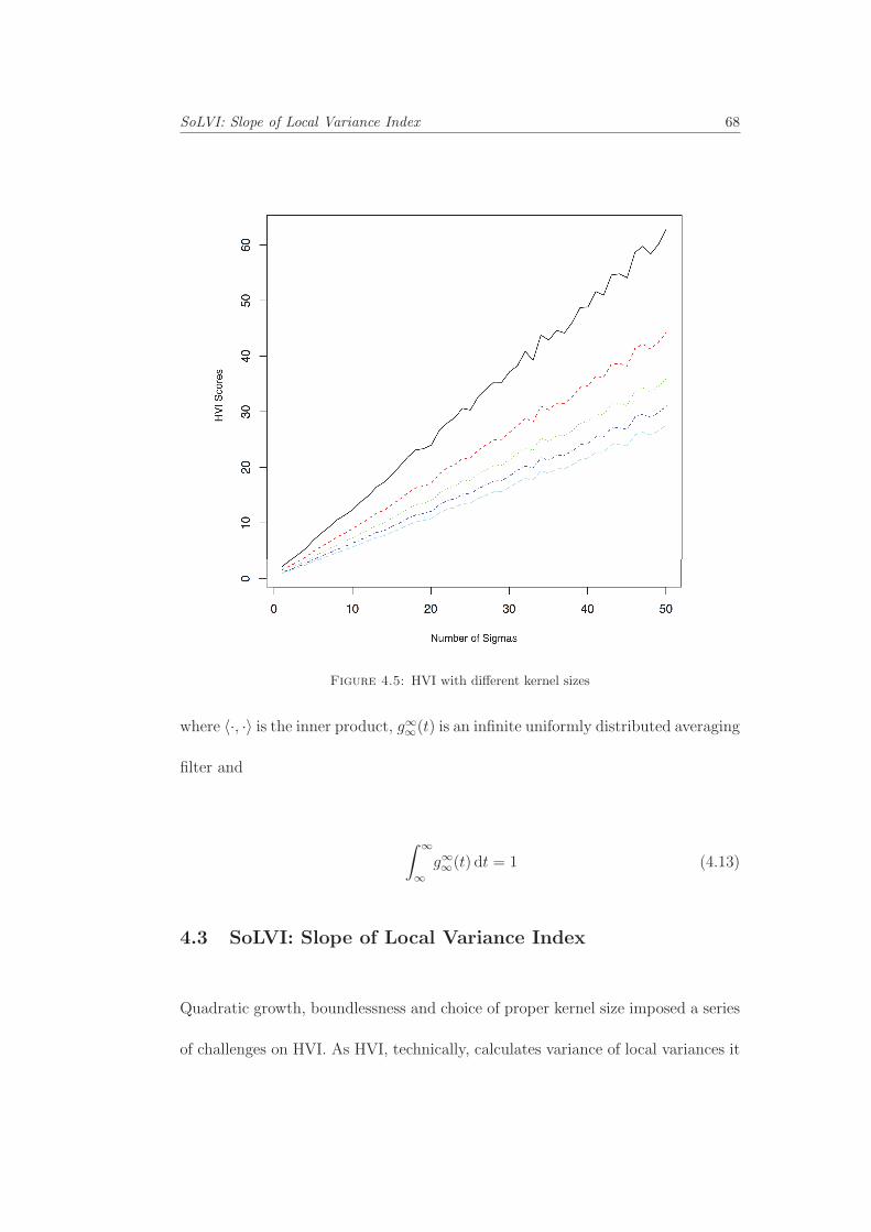
SoLVI: Slope of Local Variance Index 68
Figure 4.5: HVI with different kernel sizes
where 〈·, ·〉 is the inner product, g∞∞(t) is an infinite uniformly distributed averaging
filter and
∫ ∞
∞g∞∞(t) dt = 1 (4.13)
4.3 SoLVI: Slope of Local Variance Index
Quadratic growth, boundlessness and choice of proper kernel size imposed a series
of challenges on HVI. As HVI, technically, calculates variance of local variances it
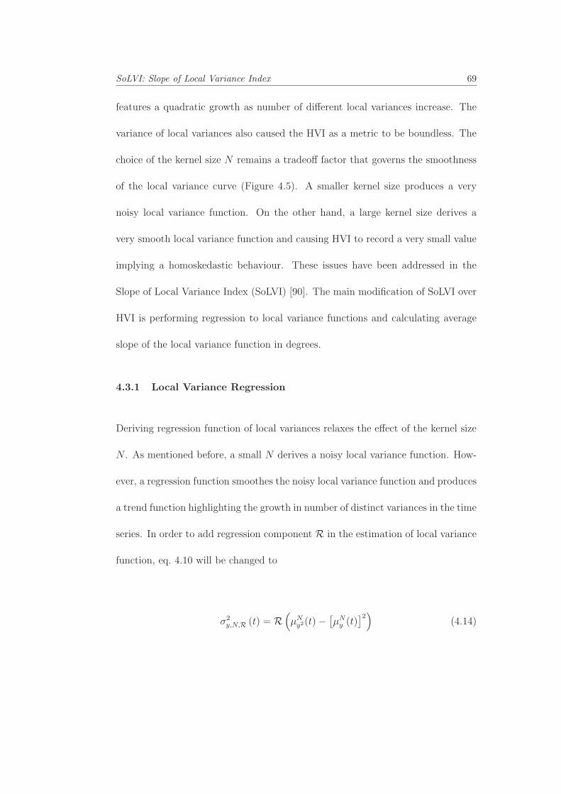
SoLVI: Slope of Local Variance Index 69
features a quadratic growth as number of different local variances increase. The
variance of local variances also caused the HVI as a metric to be boundless. The
choice of the kernel size N remains a tradeoff factor that governs the smoothness
of the local variance curve (Figure 4.5). A smaller kernel size produces a very
noisy local variance function. On the other hand, a large kernel size derives a
very smooth local variance function and causing HVI to record a very small value
implying a homoskedastic behaviour. These issues have been addressed in the
Slope of Local Variance Index (SoLVI) [90]. The main modification of SoLVI over
HVI is performing regression to local variance functions and calculating average
slope of the local variance function in degrees.
4.3.1 Local Variance Regression
Deriving regression function of local variances relaxes the effect of the kernel size
N . As mentioned before, a small N derives a noisy local variance function. How-
ever, a regression function smoothes the noisy local variance function and produces
a trend function highlighting the growth in number of distinct variances in the time
series. In order to add regression component R in the estimation of local variance
function, eq. 4.10 will be changed to
σ2y,N,R (t) = R
(μNy2(t)−
[μNy (t)
]2)(4.14)
SoLVI: Slope of Local Variance Index 70
Figure 4.6: SolVI scores for time series generated using different 64 sigmas. Thegraphs demonstrate different kernel sizes w.
4.3.2 Average Slope of Local Variance
To qualify as an index the proposed metric is then mapped between 0◦ and 90◦
using tan−1. The change of local variances is measured by estimating
mσ2y=
d
dtσ2y,N,R (t) (4.15)
SoLVI: Slope of Local Variance Index 71
and then heteroskedasticity is quantified by calculating the average tangent angle
of local variance function as
μθ(σ2y) =
1
N
∫ N
t=1
[tan−1
(d
dtR (
σ2y(t|w)
))]dt (4.16)
where θ(σ2y
)is the local tangent angles function of σ2
y(t|w), N is the length of
the time series and μθ(σ2y) is the average local tangent angles of the same function
that correlates theoretically with the change of local variances and hence quantifies
heteroskedasticity. Figure 4.6 shows SoLVI scores of synthesised heteroskedastic
data with number of standard deviations ranging from 1 to 64.
4.3.3 Selection of Kernel Size w
The application domain dictates the selection of kernel sizes w. The economist
investigating the time series should have an idea about the range of number of
variances in the time series. As illustrated in Figure 4.6, higher kernel sizes lin-
earises the SoLVI score graph. The kernel size w serves then as a parameter to
zoom in and out on a particular number of sigmas.
4.4 Conclusions
Based on our study, there are two types of metrics to measure heteroskedasticity:
local variance based metrics and statistical based metrics. Local variance based
metrics were the core of our early attempts to quantify heteroskedasticity. They

SoLVI: Slope of Local Variance Index 72
calculate the local variances in the time series. Both Heteroskedasticity variance
Index (HVI) and Slope of Local Variance Index (SoLVI) techniques can be clas-
sified under this category. HVI uses global variance of the obtained local sigmas.
The SoLVI model performs regression on local sigmas and calculates the average
slope.The proposed index provides more than just a hypothesis test. The main
advantage of the proposed metric is providing a quantifying method to test how far
a heteroskedastic series is from being homoskedastic. The results show consistency
between the proposed index and the widely popular heteroskedasticity tests.
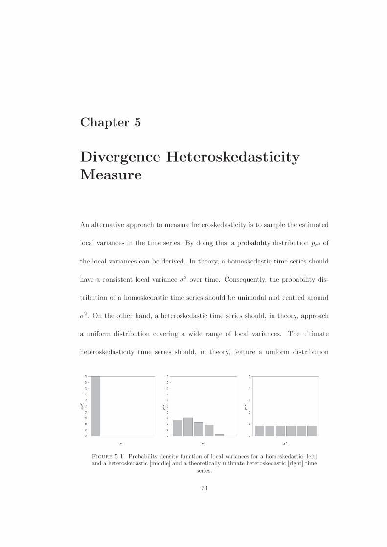
Chapter 5
Divergence HeteroskedasticityMeasure
An alternative approach to measure heteroskedasticity is to sample the estimated
local variances in the time series. By doing this, a probability distribution pσ2 of
the local variances can be derived. In theory, a homoskedastic time series should
have a consistent local variance σ2 over time. Consequently, the probability dis-
tribution of a homoskedastic time series should be unimodal and centred around
σ2. On the other hand, a heteroskedastic time series should, in theory, approach
a uniform distribution covering a wide range of local variances. The ultimate
heteroskedasticity time series should, in theory, feature a uniform distribution
Figure 5.1: Probability density function of local variances for a homoskedastic [left]and a heteroskedastic [middle] and a theoretically ultimate heteroskedastic [right] time
series.
73

Divergence Heteroskedasticity Measure 74
U (0,∞). Therefore, measuring the distance between the probability distribution
of the local variances pσ2 and the uniform distribution provides a quantified mea-
sure of heteroskedasticity. In this section, we propose heteroskedasticity measures
based on probability distribution metrics. The heteroskedasticity quantified mea-
sure is defined as follows:
H(y) = Δp
(P (σ2
y),U(0,∞))
(5.1)
where Δp : P2 → [0, 1] is a distribution distance function of the estimated local
variances σ2y .
Many probability distribution metrics are available. However, most of them rely on
entropies, joint probability density functions and sigma algebra. In this section a
justification for excluding three of the most famous probability distribution metrics
is discussed.
5.1 Mutual Information (MI)
Mutual information between two random variablesX and Y derives a cross entropy
between the joint probability distribution p(x, y) and the ultimate scenario of
complete mutual independence p(x) · p(y) as follows:
MI(X;Y ) =
∫ ∫p(x, y) log
(p(x, y)
p(x)p(y)
)dx dy (5.2)
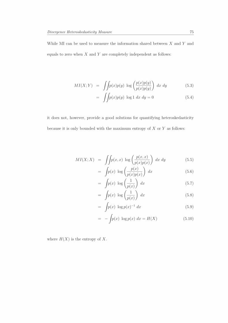
Divergence Heteroskedasticity Measure 75
While MI can be used to measure the information shared between X and Y and
equals to zero when X and Y are completely independent as follows:
MI(X;Y ) =
∫ ∫p(x)p(y) log
(p(x)p(y)
p(x)p(y)
)dx dy (5.3)
=
∫ ∫p(x)p(y) log 1 dx dy = 0 (5.4)
it does not, however, provide a good solutions for quantifying heteroskedasticity
because it is only bounded with the maximum entropy of X or Y as follows:
MI(X;X) =
∫ ∫p(x, x) log
(p(x, x)
p(x)p(x)
)dx dy (5.5)
=
∫p(x) log
(p(x)
p(x)p(x)
)dx (5.6)
=
∫p(x) log
(1
p(x)
)dx (5.7)
=
∫p(x) log
(1
p(x)
)dx (5.8)
=
∫p(x) log p(x)−1 dx (5.9)
= −∫p(x) log p(x) dx = H(X) (5.10)
where H(X) is the entropy of X.
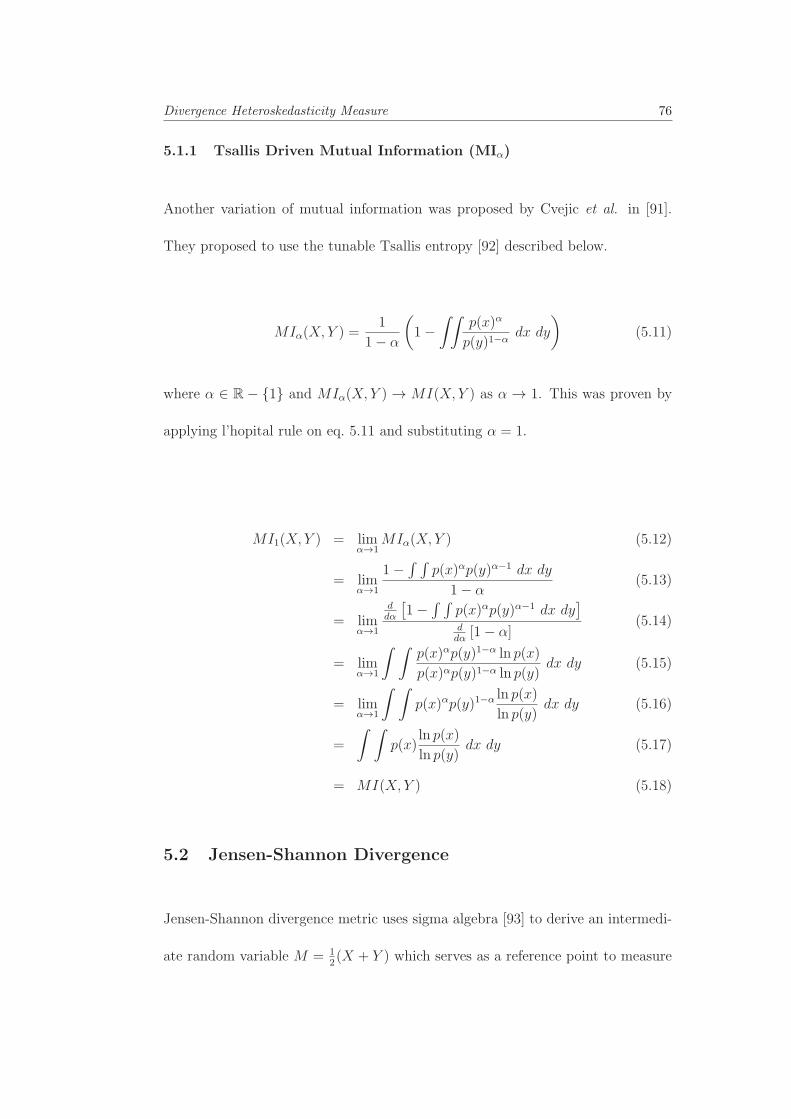
Divergence Heteroskedasticity Measure 76
5.1.1 Tsallis Driven Mutual Information (MIα)
Another variation of mutual information was proposed by Cvejic et al. in [91].
They proposed to use the tunable Tsallis entropy [92] described below.
MIα(X, Y ) =1
1− α
(1−
∫ ∫p(x)α
p(y)1−αdx dy
)(5.11)
where α ∈ R − {1} and MIα(X, Y ) → MI(X, Y ) as α → 1. This was proven by
applying l’hopital rule on eq. 5.11 and substituting α = 1.
MI1(X, Y ) = limα→1
MIα(X, Y ) (5.12)
= limα→1
1− ∫ ∫p(x)αp(y)α−1 dx dy
1− α(5.13)
= limα→1
ddα
[1− ∫ ∫
p(x)αp(y)α−1 dx dy]
ddα
[1− α](5.14)
= limα→1
∫ ∫p(x)αp(y)1−α ln p(x)
p(x)αp(y)1−α ln p(y)dx dy (5.15)
= limα→1
∫ ∫p(x)αp(y)1−α ln p(x)
ln p(y)dx dy (5.16)
=
∫ ∫p(x)
ln p(x)
ln p(y)dx dy (5.17)
= MI(X, Y ) (5.18)
5.2 Jensen-Shannon Divergence
Jensen-Shannon divergence metric uses sigma algebra [93] to derive an intermedi-
ate random variable M = 12(X + Y ) which serves as a reference point to measure

Divergence Heteroskedasticity Measure 77
distance of X and Y from using mutual information as follows:
JSD(X, Y ) =1
2MI(X,M) +
1
2MI(Y,M) (5.19)
While this metric is bounded to 0 ≤ JSD(X, Y ) ≤ 1, deriving the mixture distri-
bution of the random variable M is computationally intensive.
5.3 Renyi Divergence
Renyi divergence [94] uses a generalised form of Shannon, Hartley, min-, and
collision- entropies [95, 96] and is formulated as follows:
Hα =1
1− αlog
(∫p(x)α
)(5.20)
Renyi’s divergence metric is then formulated as follows:
Rα(X, Y ) =1
1− αlog
(∫ ∫p(x)αp(y)1−α dx dy
)(5.21)
As Reynyi entropy generalises many entropies, its divergence metric also gener-
alises many divergence metrics. For example, when α → 1 the Renyi entropy
converges to Shannon’s entropy and the divergence metric converges to the Mu-
tual Information metric by applying l’hopital rule as follows:
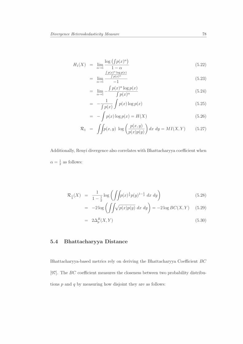
Divergence Heteroskedasticity Measure 78
H1(X) = limα→1
log(∫
p(x)α)
1− α(5.22)
= limα→1
∫p(x)α log p(x)∫
p(x)α
−1(5.23)
= limα→1
−∫p(x)α log p(x)∫
p(x)α(5.24)
= − 1∫p(x)
∫p(x) log p(x) (5.25)
= −∫
p(x) log p(x) = H(X) (5.26)
R1 =
∫ ∫p(x, y) log
(p(x, y)
p(x)p(y)
)dx dy = MI(X, Y ) (5.27)
Additionally, Renyi divergence also correlates with Bhattacharyya coefficient when
α = 12as follows:
R 12(X) =
1
1− 12
log
(∫ ∫p(x)
12p(y)1−
12 dx dy
)(5.28)
= −2 log
(∫ ∫√p(x)p(y) dx dy
)= −2 logBC(X, Y ) (5.29)
= 2ΔBp (X, Y ) (5.30)
5.4 Bhattacharyya Distance
Bhattacharyya-based metrics rely on deriving the Bhattacharyya Coefficient BC
[97]. The BC coefficient measures the closeness between two probability distribu-
tions p and q by measuring how disjoint they are as follows:
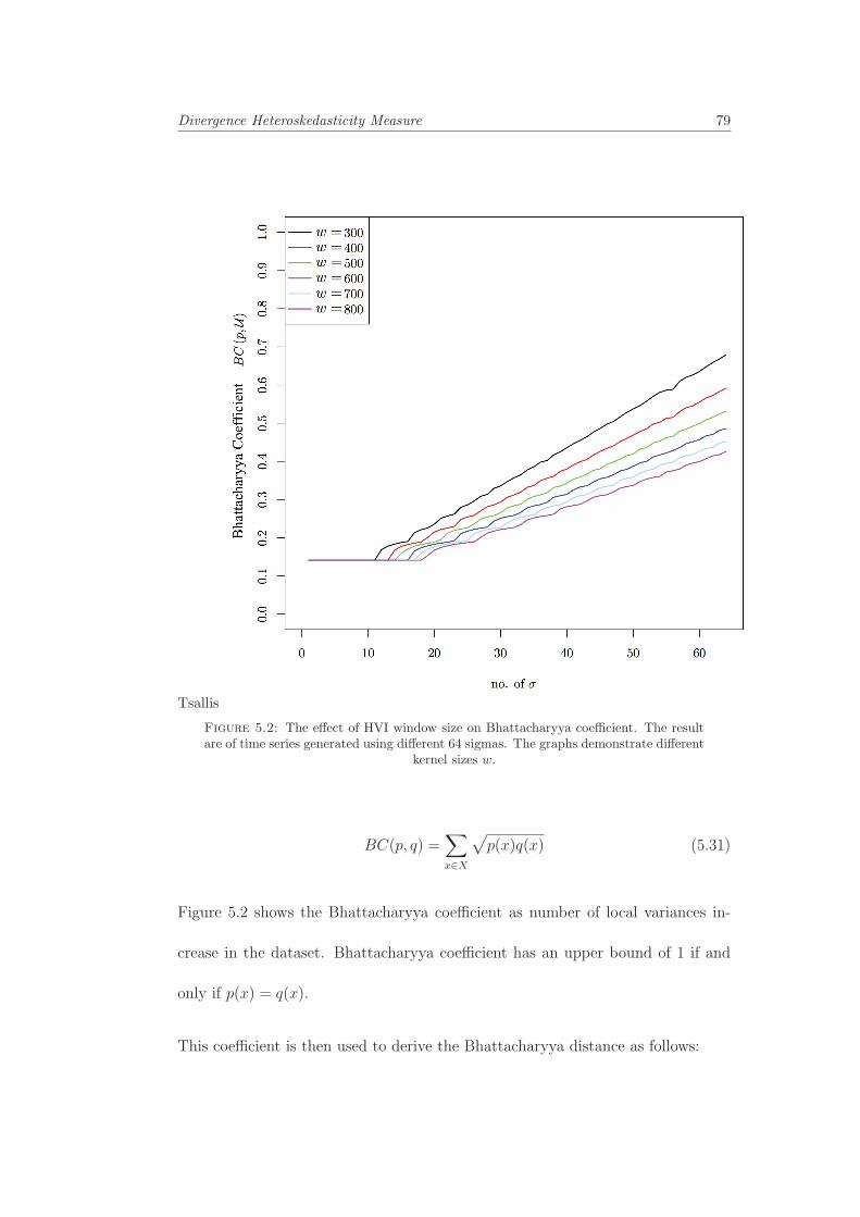
Divergence Heteroskedasticity Measure 79
Tsallis
Figure 5.2: The effect of HVI window size on Bhattacharyya coefficient. The resultare of time series generated using different 64 sigmas. The graphs demonstrate different
kernel sizes w.
BC(p, q) =∑x∈X
√p(x)q(x) (5.31)
Figure 5.2 shows the Bhattacharyya coefficient as number of local variances in-
crease in the dataset. Bhattacharyya coefficient has an upper bound of 1 if and
only if p(x) = q(x).
This coefficient is then used to derive the Bhattacharyya distance as follows:

Divergence Heteroskedasticity Measure 80
Figure 5.3: Bhattacharyya distance of a time series generated using different 64sigmas. The graphs demonstrate different kernel sizes w.
ΔBp (p, q) = − lnBC(p, q) (5.32)
However, this distance function has no upper bound and does not satisfy the
triangulation inequality. Figure 5.3 demonstrates the Bhattacharyya distance.
Divergence Heteroskedasticity Measure 81
5.4.1 Hellinger Distance
Finally, Hellinger et al. provided a sound Bhattacharyya-based divergence metric
that is bounded and satisfies the triangulation inequality in [98]. The Hellinger
metric is derived from Bhattacharyya coefficient as:
ΔHp (p, q) = 1−
√1− BC(p, q) (5.33)
Figure 5.4 shows the effect of window size on Hellinger divergence metric.
5.4.2 Bhattacharyya Heteroskedasticity Measure
As a heteroskedastic time series, by definition, is derived from systems of different
variances; the probability distribution of local variances p(σ) of a heteroskedastic
time series must be approaching a uniform distribution U . On the other hand,
a homoskedastic time series will have a probability distribution further from the
uniform distribution U . To guarantee bounded function we chose Bhattacharayya
coefficient over the Renyi driven metric in eq. 5.21. The Bhatacharayya het-
eroskedasticity measure is then formulated as follows:
HB(y) =∑x∈X
√P(σ2y
)U (σ2y
)(5.34)
where P(σ2y
)is a probability distribution function of the estimated local variances
σ2y . A Hellinger variation can also be derived with the same concept as follows:
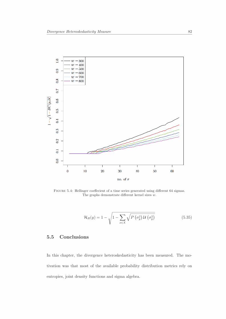
Divergence Heteroskedasticity Measure 82
Figure 5.4: Hellinger coeffecient of a time series generated using different 64 sigmas.The graphs demonstrate different kernel sizes w.
HH(y) = 1−√
1−∑x∈X
√P(σ2y
)U (σ2y
)(5.35)
5.5 Conclusions
In this chapter, the divergence heteroskedasticity has been measured. The mo-
tivation was that most of the available probability distribution metrics rely on
entropies, joint density functions and sigma algebra.

Divergence Heteroskedasticity Measure 83
Mutual information, Jensen-Shannon divergence and Renyi divergence were ex-
cluded. Consequently, the Bhattacharyya Distance was adopted to introduce
Bhattacharyya heteroskedasticity measure. The main reason behind preferring
the Bhattacharyya over the Renyi divergence model was to guarantee a bounded
function. The Bhattacharyya heteroskedasticity measure was then formulated,
with the ability to derive the Hellinger variation.
Chapter 6
Conclusions and Future Work
This chapter discusses the conclusions driven from the work presented in this thesis
and identifies rooms for future improvements and open research problems.
This study presents a novel strategy for identifying the presence and quantify-
ing heteroskedasticity in the time series, by deriving a quantifying measurement
for heteroskedasticity. The proposed measure relies on the common definition of
heteroskedasticity as a time- variant variance in the time series. This framework
enables the pre-existing models to predict this type of uncertainty, making it more
beneficial and more satisfying in predicting long-term span. In addition, a better
forecast is to be achieved to allow for a more reliable decision- making and future
planning.
Traditionally, heteroskedasticity features in time series have become a factor around
which forecasting models have to work and errors for which they must compensate.
In this work we have addressed the heteroskedasticity problem from a different per-
spective. The objective of this work is to quantify a heteroskedastic behaviour as
84
Conclusions and Future Work 85
opposed to just detecting the behaviour with heteroskedastic tests. First, an argu-
ment justifying the need for heteroskedasticity quantification rather than detection
was derived. Then, we characterised the different features that make a time se-
ries test positive to heteroskedastic tests. This characterisation is then used to
generate synthetic test data with different levels of heteroskedasticity. Finally, we
derived two families of solutions to quantify heteroskedasticity.
The first family relies on local temporal estimation of statistical parameters that
are used in two schemes. In the first scheme, the time-variant change of the esti-
mated parameters are then used for quantifying heteroskedasticity. HVI and SoLVI
algorithms described in Chapter 3 were developed under this scheme. The pro-
posed index serves as a cost function to be optimised in many fields such as ecology,
machine learning and finance. The implementation of the proposed heteroskedas-
ticity index is straightforward. It utilises statistical and signal processing functions
available in all technical computing packages such as MatlabTM, MathematicaTM
and R. Future improvement of this work will apply different nonlinear regression
methods (e.g. polynomial and neural network) to estimate local variances in order
to resolve the current limitations of heteroskedasticity tests with unpredictable
means. Similar techniques can also be applied to quantify time variant statistical
distributions which gained more interests recently because of the climate change
and its effects on different ecosystems.
The second scheme derives the distribution of the estimated local statistical pa-
rameters and employs Kullback-Leibler divergence metrics [99] for quantification.

Conclusions and Future Work 86
Bhattacharyya and mutual information metrics were employed in Chapter 4. The
second family relies on applying heteroskedasticity tests to split the time series
into homoskedastic parts. This method facilitates the study of heteroskedastic
patterns.
During this study we discovered that homoskedastic signals with time varying sta-
tistical distributions do test positively to heteroskedastic tests while maintaining
a stationarity. Quantifying heteroskedasticity via binary decomposition [100, 101]
was investigated and will be the core of future work and implementations. Fur-
ther applications in the fields of ecological studies and financial markets are to be
explored.
References
[1] T. Bollerslev, “A conditionally heteroskedastic time series model for specu-lative prices and rates of return,” The Review of Economics and Statistics,vol. 69, no. 3, pp. 542–547, 1987.
[2] R. Engle and D. F. Kraft, “Multiperiod forecast error variances of inflationestimated from ARCH models,” Applied Time Series of Economic Data, pp.293–302, 1983.
[3] A. Harvey, E. Ruiz, and E. Sentana, “Unobserved component time-seriesmodels with ARCH disturbances,” Journal of Econometrics, vol. 52, no.1-2, pp. 129–157, 1992.
[4] T. Nilsen and T. Aven, “Models and model uncertainty in the context ofrisk analysis,” Reliability Engineering & System Safety, vol. 79, no. 3, pp.309–317, 2003.
[5] W. D. Rowe, “Understanding uncertainty,” Risk Analysis, vol. 14, no. 5, pp.743–750, 1994.
[6] G. W. Parry, “The characterisation of uncertainty in probabilistic risk as-sessments of complex systems,” Reliability Engineering & System Safety,vol. 54, no. 2, pp. 119–126, 1996.
[7] J. Helton, “Treatment of uncertainty in performance assessments for complexsystems,” Risk Analysis, vol. 14, no. 4, pp. 483–511, 1994.
[8] G. Raadgever, C. Dieperink, P. Driessen, A. Smit, and H. Van Rijswick,“Uncertainty management strategies: Lessons from the regional implemen-tation of the water framework directive in the netherlands,” EnvironmentalScience & Policy, vol. 14, no. 1, pp. 64–75, 2011.
[9] S. C. Hora, “Aleatory and epistemic uncertainty in probability elicitationwith an example from hazardous waste management,” Reliability Engineer-ing & System Safety, vol. 54, no. 2, pp. 217–223, 1996.
87
References 88
[10] F. O. Hoffman and J. S. Hammond, “Propagation of uncertainty in riskassessments: the need to distinguish between uncertainty due to the lack ofknowledge and due to variability,” Risk Analysis, vol. 14, no. 5, pp. 707–712,1994.
[11] S. Rai, D. Krewski, and S. Bartlett, “A general framework for the analysisof uncertainty and variability in risk assessment,” Human and ecological riskassessment, vol. 2, no. 4, pp. 972–989, 1996.
[12] M. E. Pate-Cornell, “Uncertainties in risk analysis: six levels of treatment.”Reliability Engineering & System Safety, vol. 54, no. 2, pp. 95–111, 1996.
[13] W. L. Oberkampf, K. V. Diegert, K. Alvin, and B. M. Rutherford, “Variabil-ity, uncertainty, and error in computational simulation,” American Societyof Mechanical Engineers- Publications- Heat Transfer Division, vol. 32, no. 2,pp. 135–154, 1998.
[14] D. Hobson, “Stochastic volatility model,” Mathematical Finance, vol. 14,no. 4, pp. 537–556, 2004.
[15] R. Cont, Frontiers in quantitative finance : volatility and credit risk model-ing, ser. Wiley finance. Hoboken, N.J.: John Wiley & Sons, 2009.
[16] R. Cont and P. Tankov, Financial modelling with jump processes, ser. finan-cial mathematics series, 2004.
[17] A. C. Harvey, Dynamic models for volatility and heavy tails : with applica-tions to financial and economic time series, ser. Econometric society mono-graphs, 2013.
[18] R. Cont, Volatility Clustering in Financial Markets: Empirical Facts andAgent-based Models. Springer Berlin Heidelberg, 2007, pp. 289–309.
[19] R. Engle, “Autoregressive conditional heteroskedasticity with estimates ofthe variance of united kingdom inflation,” Econometrica, vol. 50, no. 4, pp.987–1007, 1982.
[20] ——, “Estimates of the variance of u.s. inflation based upon the ARCHmodel,” Journal of Money, Credit and Banking, vol. 15, no. 3, pp. 286–301,1983.
[21] L. Bauwens, C. M. Hafner, and S. Laurent, Handbook of volatility modelsand their applications. Wiley, March 2012.
References 89
[22] T. Bollerslev, R. Y. Chou, and K. F. Kroner, “ARCH modelling in finance- a review of the theory and empirical evidence,” Journal of Econometrics,vol. 52, no. 1-2, pp. 5–59, 1992.
[23] C. Alexander, “Principal component models for generating large GARCHcovariance matrix,” Economic Notes, vol. 31, no. 2, pp. 337–349, 2002.
[24] L. Bauwens, S. Laurent, and J. V. K. Rombouts, “Multivariate GARCHmodels: a survey,” Journal of Applied Econometrics, vol. 21, no. 1, pp. 79–109, 2006.
[25] R. F. Engle and M. E. Sokalska, “Forecasting intraday volatility in the usequity market. multiplicative component GARCH, type = Journal Article,volume = 10, year = 2012,” Journal of Financial Econometrics, no. 1, pp.54–83.
[26] P. R. Hansen and A. Lunde, “A forecast comparison of volatility models:does anything beat a GARCH (1,1)?” Journal of Applied Econometrics,vol. 20, no. 7, pp. 873–889, 2005.
[27] M. Higgins, “A class of nonlinear ARCH models,” International EconomicReview, vol. 33, no. 1, pp. 137–158, 1992.
[28] S. Hwang, V. Pereira, and L. Pedro, “The effects of structural breaks inARCH and GARCH parameters on persistence of GARCH models,” Com-munications in Statistics - Simulation and Computation, vol. 37, no. 3, pp.571–578, 2008.
[29] C. Francq and J.-M. Zakoian, GARCH models : structure, statistical infer-ence, and financial applications. Chichester, West Sussex: Wiley, 2010.
[30] R. Engle, S. M. Focardi, and F. J. Fabozzi, ARCH/GARCH models in Ap-plied Financial Econometrics. Wiley, 2008.
[31] R. Plackett, “Some theorems in least squares,” Biometrika, vol. 37, no. (1-2),pp. 149–157, 1950.
[32] P. Galeano and R. S. Tsay, “Shifts in individual parameters of a GARCHmodel,” Journal of Financial Econometrics, vol. 8, no. 1, pp. 122–153, 2010.
[33] J. D. Hamilton, Time Series Analysis. Princeton University, 1994.

References 90
[34] A. C. Harvey, Time series models, 2nd ed. Cambridge, Mass.: MIT Press,1993.
[35] M. Hassan, M. Hossny, S. Nahavandi, and D. Creighton, “Heteroskedasticityvariance index,” IEEE Internationl Conference on Modelling and Simulation2012, pp. 135–141.
[36] J. Duan, S. Luo, and C. Wang, Recent development in stochastic dynamicsand stochastic analysis, ser. Interdisciplinary mathematical sciences. Sin-gapore ; London: World Scientific, 2010.
[37] C. Chatfield, Problem solving : a statistician’s guide, 2nd ed., ser. Chapman& Hall texts in statistical science series. London ; New York: Chapman &Hall, 1995.
[38] ——, The analysis of time series : an introduction, 6th ed., ser. Texts instatistical science. Boca Raton, FL: Chapman & Hall/CRC, 2004.
[39] G. Box, G. M. Jenkins, and G. C. Reinsel, Time series analysis : forecastingand control, 4th ed., ser. Wiley series in probability and statistics. Hoboken,N.J.: John Wiley, 2008.
[40] C. R. Plott and S. Sunder, “Efficiency of experimental security markets withinsider information: An application of rational- expectations models,” TheJournal of Political Economy, vol. 90, no. 4, pp. 668–698, 1982.
[41] G. Samoridnitsky and M. Taqqu, Stable Non-Gaussian Random Processes:Stochastic Models with Infinite Variance. Chapman and Hall, 1994.
[42] J. Nolan, “Numerical calculation of densities and distribution functions,”Stochastic Models, vol. 13, no. 4, pp. 759–774, 1997.
[43] J. P. Nolan, Stable Distributions - Models for Heavy Tailed Data. Boston:Birkhauser, 2015.
[44] J. Chambers, C. Mallows, and B. Stuck, “A method for simulating stablerandom variables,” J. Amer. Statist. Assoc., vol. 71, pp. 340–344, 1976.
[45] J. L. Knight and S. Satchell, “Forecasting volatility in the financial markets,”pp. viii, 415 p. ill. 25 cm., 2007.
[46] G. Box and G. Jenkins, Time Series Analysis: Forecasting and Control,4th ed. Wiley, 1970, vol. 734.
References 91
[47] E. M. Lin, C. W. Chen, and R. Gerlach, “Forecasting volatility with asym-metric smooth transition dynamic range models forecasting volatility withasymmetric smooth transition dynamic range models,” International Jour-nal of Forecasting, vol. 28, no. 2, pp. 384–399, June 2012.
[48] T. J. Brailsford and R. W. Faff, “An evaluation of volatility forecastingtechniques,” Journal of Banking and Finance, vol. 20, no. 3, pp. 419–438,1996.
[49] T. Bollerslev and T. G. Andersen, “Modelling and forecasting realisedvolatility,” Econometrica, vol. 71, no. 2, pp. 579–625, 2003.
[50] J. Engelberg, C. F. Manski, and J. Williams, “Comparing the point pre-dictions and subjective probability distributions of professional forecasters,”Journal of Business and Economic Statistics, vol. 27, no. 1, pp. 30–41, 2009.
[51] S. Pellegrini, E. Ruiz, and A. Espasa, “Conditionally heteroskedastic unob-served component models and their reduced form,” Economics Letters, vol.107, no. 2, pp. 88–90, 2010.
[52] ——, “Prediction intervals in conditionally heteroskedastic time series withstochastic components,” International Journal of Forecasting, vol. 27, pp.308–319, April-June 2011.
[53] A. C. Harvey, The econometric analysis of time series, 1st ed., ser. LSEhandbooks in economics. Cambridge, Mass.: MIT Press, 1990.
[54] R. Engle, “GARCH 101: The use of ARCH/GARCH models in appliedeconometrics,” Journal of Economic Perspectives, vol. 15, no. 4, pp. 157–168, 2001.
[55] T. Bollerslev, “Generalized autoregressive conditional heteroskedasticity,”Journal of Econometrics, vol. 100, no. 1, pp. 307–327, 1986.
[56] T. Busch, “A robust LR test for the GARCH model,” Economics Letters,vol. 88, pp. 358–364, 2005.
[57] D. B. Nelson and C. Q. Cao, “Inequality constraints in the univariateGARCH model,” Journal of Business and Economic Statistics, vol. 10, no. 2,pp. 229–235, 1992.
[58] J. Duan, “Augmented GARCH (p,q) process and its diffusion limit,” Journalof Econometrics, vol. 79, no. 1, pp. 97–127, 1997.

References 92
[59] C. G. Lamoureux and W. D. Lastrrapes, “Heteroskedasticity in stock returndata: Volume versus GARCH effects,” Journal of Finance, vol. 45, no. 1,pp. 221–229, 1990.
[60] S. J. Taylor, Modelling Financial Time Series. World Scientific, 2008.
[61] R. F. Engle and V. K. NG, “Measuring and testing the impact of news onvolatility,” The Journal of Finance, vol. 48, no. 5, pp. 1749–1778, 1993.
[62] L. Hentshel, “All in the family: Nesting symmetric and asymmetric GARCHmodels,” Journal of Financial Economics, vol. 39, pp. 71–104, 1995.
[63] V. Barnett and T. Lewis, Outliers in Statistical Data, 3rd ed. Wiley, 1994.
[64] H. Liu, S. Shah, and W. Jiang, “On-line outlier detection and data cleaning,”Computers and Chemical Engineering, vol. 28, no. 9, pp. 1635–1647, 2004.
[65] Y. Chen, D. Miao, and H. Zhang, “Neighborhood outlier detection,” ExpertSystems with Applications, vol. 37, pp. 8745–8749, 2010.
[66] I. Morgan, “Stock prices and heteroskedasticity,” Journal of Business andEconomic Statistics, vol. 49, pp. 496–508, 1976.
[67] A. Harvey and G. Phillips, “A comparison of the power of some tests forheteroskedasticity in the general linear model,” Journal of Econometrics,vol. 2, no. 4, pp. 307–316, 1974.
[68] S. Goldfeld and R. Quandt, “Some tests for homoskedasticity,” Journal ofthe American Statistical Association, vol. 60, no. 310, pp. 539–547, 1965.
[69] H. Glejser, “A new test for heteroskedasticity,” Journal of the AmericanStatistical Association, vol. 64, no. 325, pp. 316–323, 1969.
[70] R. E. Park, “Estimation with heteroskedastic error terms,” Econometrica,vol. 34, no. 4, 1966.
[71] D. A. Bowers and H. C. Rutemiller, “Estimation in a heteroskedastic regres-sion model,” Journal of the American Statistical Association, vol. 63, no.332, pp. 552–557, 1968.
[72] J. Harvey, M. K. Johnson, and J. Harvey, Modern economics. Study guideand workbook, 5th ed. Basingstoke: Macmillan Education, 1989.

References 93
[73] Y. Honda, “Testing the error components model with non-normal distur-bance,” The Review of Economic Studies, vol. 52, no. 4, pp. 681–690, 1985.
[74] D. Cox and D. Hinkley, Theoretical Statistics, 1st ed., 1979.
[75] J. D. Lyon and C.-L. Tsai, “A comparison of tests for heteroskedasticity,”Journal of the Royal Statistical Society Series D ( The Statistician), vol. 45,no. 3, pp. 337–349, 1996.
[76] D. Cox and N. Reid, “Parameter orthogonality and approximate conditionalinference,” Journal of the Royal Statisical Society Series B: Methodological,vol. 49, no. 1, pp. 1–39, 1987.
[77] A. P. Verbyla, “Modelling variance heterogeneity: Residual maximum like-lihood and diagnostics,” Journal of the Royal Statistical Society Series B:Methodological, vol. 55, no. 2, pp. 493–508, 1993.
[78] T. S. Breusch and A. R. Pagan, “Simple test for heteroskedasticity andrandom coefficient variation,” Econometrica, vol. 47, no. 5, pp. 1278–1294,1979.
[79] H. White, “A heteroskedasticity-consistent covariance matrix estimator anda direct test for heteroskedasticity,” Econometrica, vol. 48, no. 4, pp. 817–838, 1980.
[80] H. Levene, “In contributions to probability and statistics: Essays in honourof harold hotelling,” Stanford University Press, pp. 278–292, 1960.
[81] R. T. Baillie and T. Bollerslev, “Prediction in dynamic models with time-dependent conditional variances,” Journal of Econometrics, vol. 52, pp. 91–113, 1992.
[82] A. Khosravi, S. Nahavandi, and D. Creighton, “Construction of optimalprediction intervals for load forecasting problems,” IEEE transactions onPower systems, vol. 25, no. 1496-1503, 2010.
[83] ——, “A prediction interval-based approach to determine optimal structuresof neural network metamodels,” Expert Systems with Applications, vol. 37,no. 3, pp. 2377–2387, 2010.
[84] A. Khosravi, S. Nahavandi, D. Creighton, and A. Atiya, “Comprehensive re-view of neural network-based prediction intervals and new advances,” IEEETransactions on Neural Networks, vol. 22, pp. 1341–1356, 2011.
References 94
[85] A. Khosravi, S. Nahavandi, D. Creighton, and R. Naghavizadeh, “Uncer-tainty quantification for wind farm power generation,” Proceedings of theIEEE International Joint Conference on Neural Networks, pp. 309–314, June2012.
[86] M. Hossny, S. Nahavandi, and D. Creighton, “Comments on informationmeasure for performance of image fusion,” Electronics Letters, vol. 44, no. 28,pp. 1066–1067, 2008.
[87] M. Hossny and S. Nahavandi, “Measuring the capacity of image fusion,”in IEEE International Conference on Image Processing Theory,Tools andApplications (IPTA), October 2012, pp. 415–420.
[88] M. Hossny, S. Nahavandi, and D. Creighton, “An evaluation mechanism forsaliency functions used in localized image fusion quality metrics,” in IEEEConference on Computer Modelling and Simulation, March 2012, pp. 407–415.
[89] T. S. Breusch and A. R. Pagan, “The lagrange multiplier test and its ap-plications to model specification in econometrics,” The Review of EconomicStudies, vol. 47, no. 1, pp. 239–253, 1980.
[90] M. Hassan, M. Hossny, S. Nahavandi, and D. Creighton, “Quantifying het-eroskedasticity using slope of local variances index,” IEEE InternationalConference on Modelling and Simulation, no. 107-111, April 2013.
[91] N. Cvejic, C. Canagarajah, and D. Bull, “Image fusion metric based onmutual information and tsallis entropy,” Electronics Letters, vol. 42, no. 11,pp. 626–627, 2006.
[92] C. Tsallis, “Possible generalization of Boltzmann-Gibbs statistics,” Journalof Statistical Physics, vol. 52, pp. 479–487, 1988.
[93] T. Fischer, “On simple representations of stopping times and stopping timesigma-algebras,” Statistics and Probability Letters, vol. 83, no. 1, pp. 345–349, 2013.
[94] A. Renyi, “On measures of information and entropy,” Proceedings of thefourth Berkeley Symposium on Mathematics, Statistics and Probability, pp.547–561, 1960.
[95] C. E. Shannon, “A mathematical theory of communication,” Bell SystemTechnical Journal, vol. 27, no. 3, p. 379423, 1948.

References 95
[96] R. Knig, R. Renner, and C. Schaffner, “The operational meaning of min-andmax-entropy,” IEEE Transactions on Information Theory, vol. 55, no. 9, pp.4337–4347, 2009.
[97] A. Bhattacharyya, “On a measure of divergence between two statistical pop-ulations defined by their probability distributions,” Bulletin of the CalcuttaMathematical Society, vol. 35, pp. 99–109, 1943.
[98] E. Hellinger, “Neue begrndung der theorie quadratischer formen von un-endlichvielen vernderlichen,” Journal fr die reine und angewandte Mathe-matik, vol. 136, pp. 210–271, 1909.
[99] R. Dahlhaus, “On the kullback-leibler information divergence of locally sta-tionary processes,” Stochastic processes and their applications, vol. 62, no. 1,pp. 139–168, March 1996.
[100] M. Hassan, M. Hossny, S. Nahavandi, and D. Creighton, “Quantifying het-eroskedasticity via binary decomposition,” IEEE International Conferenceon Modelling and Simulation, pp. 112–116, 2013.
[101] M. Hossny, S. Nahavandi, D. Creighton, and M. Hassan, “Image fusion met-rics: Evolution in a nutshell,” IEEE International Conference on ComputerModelling and Simulation, pp. 443–450, 2013.