Remote Sensing of Environment 123 (2012) 25–40

Contents lists available at SciVerse ScienceDirect

Remote Sensing of Environment

j ourna l homepage: www.e lsev ie r .com/ locate / rse

Quantifying aboveground forest carbon pools and fluxes from repeat LiDAR surveys

Andrew T. Hudak a,⁎,1, Eva K. Strand b,1, Lee A. Vierling b, John C. Byrne a, Jan U.H. Eitel b,c,Sebastián Martinuzzi d, Michael J. Falkowski e

a Rocky Mountain Research Station, United States Forest Service, Moscow, ID, United Statesb Forest, Rangeland, and Fire Sciences, University of Idaho, Moscow, ID, United Statesc McCall Outdoor Science School, University of Idaho, McCall, ID, United Statesd Forest and Wildlife Ecology, University of Wisconsin, Madison, WI, United Statese School of Forest Resources and Environmental Science, Michigan Technological University, United States

⁎ Corresponding author. Tel.: +1 208 883 2327; fax:E-mail address: ahudak@fs.fed.us (A.T. Hudak).

1 Equally contributing authors.

0034-4257/$ – see front matter. Published by Elsevier Idoi:10.1016/j.rse.2012.02.023

a b s t r a c t

a r t i c l e i n f o

Article history:Received 31 October 2011Received in revised form 23 February 2012Accepted 25 February 2012Available online 5 April 2012

Keywords:Discrete return LiDARMulti-temporalAboveground carbonMixed conifer forestRandom forest algorithmImputationBiomass changeCarbon Measuring Reporting and Verification(MRV)

Sound forest policy and management decisions to mitigate rising atmospheric CO2 depend upon accuratemethodologies to quantify forest carbon pools and fluxes over large tracts of land. LiDAR remote sensing isa rapidly evolving technology for quantifying aboveground biomass and thereby carbon pools; however, littlework has evaluated the efficacy of repeat LiDAR measures for spatially monitoring aboveground carbon poolsthrough time. Our study objective was therefore to evaluate the use of discrete return airborne LiDAR forquantifying biomass change and carbon flux from repeat field and LiDAR surveys. We collected LiDAR datain 2003 and 2009 across ~20,000 ha of an actively managed, mixed conifer forest landscape in northernIdaho. The Random Forest machine learning algorithm was used to impute aboveground biomass pools oftrees, saplings, shrubs, herbaceous plants, coarse and fine woody debris, litter, and duff using field-basedforest inventory data and metrics derived from the LiDAR collections. Separate predictive tree abovegroundbiomass models were developed from the 2003 and 2009 field and LiDAR data, and biomass change was es-timated at the plot, pixel, and landscape levels by subtracting 2003 predictions from 2009 predictions. Tradi-tional stand exam data were used to independently validate 2003 and 2009 tree aboveground biomasspredictions and tree aboveground biomass change estimates at the stand level. Over this 6-year period, wefound a mean increase in tree aboveground biomass due to forest growth across the non-harvested portionsof 4.1 Mg/ha/yr. We found that 26.3% of the landscape had been harvested during this time period whichoutweighed growth at the landscape level, resulting in a net tree aboveground biomass change of−5.7 Mg/ha/yr, and −2.3 Mg/ha/yr in total aboveground carbon, summed across all the abovegroundbiomass pools. Change in aboveground biomass was related to forest successional status; younger standsgained two- to three-fold less biomass than did more mature stands. This result suggests that even themost mature forest stands are valuable carbon sinks, and implies that forest management decisions thatinclude longer harvest rotation cycles are likely to favor higher levels of aboveground carbon storage inthis system. A 30-fold difference in LiDAR sampling density between the 2003 and 2009 collections did notaffect plot-scale biomass estimation. These results suggest that repeat LiDAR surveys are useful foraccurately quantifying high resolution, spatially explicit biomass and carbon dynamics in conifer forests.

Published by Elsevier Inc.

1. Introduction

Forests cover approximately one third of the Earth's land surfaceand have a tremendous capacity to store and cycle carbon (e.g.Dixon et al., 1994; Harmon & Marks, 2002). Indeed, the total carbonstored in forested ecosystems, including live and dead wood, litter,detritus, and soil, exceeds the amount of carbon found in theatmosphere (FRA, 2005; Heath et al., 2010). Accelerated pressure onforest resources to provide a wide range of environmental services,

+1 208 883 2318.

nc.

including mitigation of atmospheric carbon dioxide, has given riseto concerted study of how change in forest cover and land use affectsemissions of CO2 to the atmosphere (McKinley et al., 2011), and howforests may be managed for carbon benefits (Hines et al., 2010).Because forest change is a highly dynamic, broad scale phenomenon,such efforts to understand the carbon balance of forests via frame-works such as the Reduction of Emissions from Deforestation andforest Degradation (REDD; e.g. Gibbs et al., 2007) in developingnations and through various other carbon Measuring, Reporting,and Verification (MRV) protocols require repeatable, objective, andaccurate remote sensing methods for estimating aboveground forestcarbon pools and fluxes over large areas (Goetz & Dubayah, 2011).Improved quantitative methods at the landscape level, where forest

26 A.T. Hudak et al. / Remote Sensing of Environment 123 (2012) 25–40

management decisions are made, could lead to more accurate forestcarbon accounting at the national level, where policy decisions aremade (Heath et al., 2010; Hines et al., 2010).

Remote sensing approaches for quantifying components of forestbiomass are rapidly evolving. Vine and Sathaye (1997) suggestedthat to quantify aboveground forest carbon pools and fluxes acrossbroad extents, it is important to combine remote sensing techniqueswith carbon estimation methods that are based on existing standardforest inventory principles. Light Detection And Ranging (LiDAR)has been employed to successfully quantify vertical structure and for-est attributes such as canopy height distribution, tree height, andcrown diameter (e.g. Hudak et al., 2002; Lefsky et al., 2002; Nilsson,1996; Yu et al., 2008). Robust methods for producing wall-to-wallmaps of aboveground forest carbon pools using single-date LiDARcombined with field data collections and Monte Carlo statisticalmethods have recently been developed with errors b1% (Gonzalezet al., 2010). Single-date LiDAR combined with field data and satelliteimagery was used to quantify carbon pools at high spatial resolutionat the landscape level (~106 ha) in Hawaii (Asner et al., 2011), and re-cently, spaceborne LiDAR was used in combination with spaceborneradar and MODIS data to quantify tropical carbon stocks acrossthree continents (Saatchi et al., 2011).

Observing landscape level changes in carbon pools (i.e. carbonfluxes) at high spatial resolution requires repeat acquisition of LiDARdata via aircraft or satellite sensors. However, few studies have used re-peat LiDAR acquisitions for any purpose. Dubayah et al. (2010) usedrepeat collections of waveform LiDAR data from the NASA Laser Vege-tation Imaging Sensor (LVIS) instrument in 1998 and 2005 to deter-mine change in forest height in a humid tropical forest of Costa Rica,and were able to infer whether primary and secondary tropical forestswere sources, sinks, or neutral with respect to their carbon emissionsduring the intervening time interval. Bater et al. (2011) assessed thereproducibility of height and intensity metrics derived from multipleLiDAR acquisitions of coniferous forest on Vancouver Island collectedon the same day and found that most metrics provided stable repeatedmeasures of forest structure. Yu et al. (2004) applied an automated,object-oriented tree-matching algorithm to two LiDAR acquisitions col-lected two years apart to estimate height growth of ~5 cm at the standlevel and 10–15 cm at the plot level. These studies show promise formulti-temporal LiDAR based assessment of forest dynamics and carbonflux. However, as LiDAR technology continues to evolve, much addi-tional work is needed to extend this approach and narrow uncer-tainties in the quantification of forest carbon dynamics. Of particularimportance are areas of active forest management (e.g., timberharvest) comprised of different forest successional and structuralstages (Falkowski et al., 2009). Understanding biomass and carbondynamics across varied forest management and successional regimesis highly useful for predictive modeling and carbon managementbecause it connects forest ecosystem processes such as growth andharvest with landscape-level carbon pools and fluxes.

The primary objective of this research is to utilize repeat LiDARand field plot surveys and statistical modeling to predict biomasspools and estimate rates of aboveground carbon flux in managedmixed conifer forests of the Northern Rocky Mountains, USA. Specifi-cally, we utilize field forest inventory data and airborne LiDAR datacollected during the summers of 2003 (Hudak et al., 2006) and2009 to quantify the effects of forest growth and timber harvest oncarbon pools of trees, saplings, shrubs, coarse and fine woody debris,herbaceous plants, litter, and duff across an actively managed forestlandscape, and examine relationships among changes in these poolsduring this 6-year interval with respect to forest height and succes-sional status. The study serves a broader objective of demonstratinga repeatable methodology for inventory and monitoring of forest car-bon pools and fluxes across actively managed forest landscapes tosupport much needed carbon measuring, reporting, and verificationmethodologies over time.

2. Methods

2.1. Study area

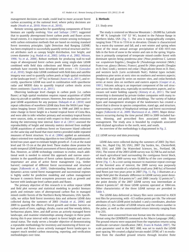
The study is centered on Moscow Mountain (~20,000 ha; Latitude46° 48′ N, Longitude 116° 52′ W), located in the Palouse Range inNorthern Idaho, USA (Fig. 1). The area is topographically complex,ranging from 770 m to 1516 m in elevation. Climate is characterizedby a warm dry summer and fall, and a wet winter and spring whenmost of the mean annual average precipitation of 630–1015 mmfalls in the form of snow in the winter and rain in the spring. Vegeta-tion is primarily comprised of temperate mixed-conifer forest withdominant species being ponderosa pine (Pinus ponderosa C. Lawsonvar. scopulorum Engelm.), Douglas-fir (Pseudotsuga menziesii (Mirb.)Franco var. glauca (Beissn.) Franco), grand fir (Abies grandis (Douglasex D. Don) Lindl.), western red cedar (Thuja plicata Donn ex D. Don),and western larch (Larix occidentalis Nutt). Habitat types include:ponderosa pine series at xeric sites on southern and western aspects;Douglas-fir and grand fir series on moister sites, and cedar/hemlockseries at mesic sites on northern and eastern aspects (Cooper et al.,1991). Volcanic ashcap is an important component of the soil struc-ture across the study area, especially on northeastern aspects, and in-creases soil water holding capacity (Kimsey et al., 2011). The landownership is dominated by private timber companies with many in-terspersed private and public land inholdings. The variety of habitattypes and management strategies of the landowners has created aforest that is diverse in species composition, stand age, and structure,representing a variety of biophysical settings and forest successionalstages (Falkowski et al., 2009; Martinuzzi et al., 2009). Major distur-bances occurring during the time period 2003 to 2009 included har-vest, thinning, and prescribed fires associated with forestmanagement. The study area is bounded by croplands associatedwith dryland agriculture to the north, west, and south.

An overview of the methodology is diagrammed in Fig. 2.

2.2. LiDAR surveys and data processing

LiDAR data were collected during the summers of 2003 (by Hori-zons, Inc., Rapid City, SD, USA), 2007 (by Surdex, Inc., Chesterfield,MO, USA) and 2009 (by Watershed Sciences, Inc., Portland, OR,USA). The extent of the 2003 LiDAR survey was 32,708 ha and includ-ed much agricultural land surrounding the contiguous forest block,while that of the 2009 survey was 19,889 ha of the core contiguousforest (Fig. 1). As a cost-saving measure to maximize repeat coverageof the forested area of interest, the 2009 survey was purposelycontracted to be outside of a relatively small area (840 ha) of forestedland flown just two years prior in 2007 (Fig. 1). Fig. 3 illustrates at asingle field plot the dramatic difference in LiDAR survey point densi-ties between 2003 (0.4 points/m2) and 2009 (nearly 12 points/m2);the point density of the 2007 LiDAR survey was intermediate atalmost 6 points/m2. All three LiDAR systems operated at 1064 nm.Other characteristics of the three LiDAR surveys are provided inTable 1.

The LiDAR data delivered as binary files were converted to ASCIItext files for processing, with ~0.5 million points per tile. The relevantattributes of each LiDAR point included: x and y coordinates, absoluteelevation (z), the number of LiDAR returns and the return number inthe pulse, as well as the unnormalized return intensity ranging from0 to 255.

Points were converted from text format into the ArcInfo coverageformat using the GENERATE command in Arc Macro Language (AML).The ground returns were separated from the vegetation returns usingmultiscale curvature classification (MCC, Evans & Hudak, 2007). Thescale parameter used in the MCC AML was set to match the LiDARpost-spacing. We created a digital terrain model (DTM) of 1 m resolu-tion from the classified ground returns through iterative finite

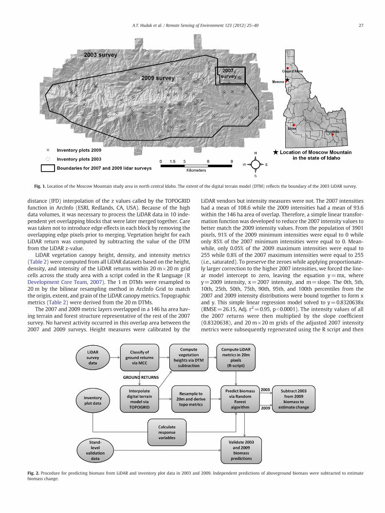
Fig. 1. Location of the Moscow Mountain study area in north central Idaho. The extent of the digital terrain model (DTM) reflects the boundary of the 2003 LiDAR survey.

27A.T. Hudak et al. / Remote Sensing of Environment 123 (2012) 25–40

distance (IFD) interpolation of the z values called by the TOPOGRIDfunction in ArcInfo (ESRI, Redlands, CA, USA). Because of the highdata volumes, it was necessary to process the LiDAR data in 10 inde-pendent yet overlapping blocks that were later merged together. Carewas taken not to introduce edge effects in each block by removing theoverlapping edge pixels prior to merging. Vegetation height for eachLiDAR return was computed by subtracting the value of the DTMfrom the LiDAR z-value.

LiDAR vegetation canopy height, density, and intensity metrics(Table 2) were computed from all LiDAR datasets based on the height,density, and intensity of the LiDAR returns within 20 m×20 m gridcells across the study area with a script coded in the R language (RDevelopment Core Team, 2007). The 1 m DTMs were resampled to20 m by the bilinear resampling method in ArcInfo Grid to matchthe origin, extent, and grain of the LiDAR canopymetrics. Topographicmetrics (Table 2) were derived from the 20 m DTMs.

The 2007 and 2009 metric layers overlapped in a 146 ha area hav-ing terrain and forest structure representative of the rest of the 2007survey. No harvest activity occurred in this overlap area between the2007 and 2009 surveys. Height measures were calibrated by the

Fig. 2. Procedure for predicting biomass from LiDAR and inventory plot data in 2003 andbiomass change.

LiDAR vendors but intensity measures were not. The 2007 intensitieshad a mean of 108.6 while the 2009 intensities had a mean of 93.6within the 146 ha area of overlap. Therefore, a simple linear transfor-mation function was developed to reduce the 2007 intensity values tobetter match the 2009 intensity values. From the population of 3901pixels, 91% of the 2009 minimum intensities were equal to 0 whileonly 85% of the 2007 minimum intensities were equal to 0. Mean-while, only 0.05% of the 2009 maximum intensities were equal to255 while 0.8% of the 2007 maximum intensities were equal to 255(i.e., saturated). To preserve the zeroes while applying proportionate-ly larger correction to the higher 2007 intensities, we forced the line-ar model intercept to zero, leaving the equation y=mx, wherey=2009 intensity, x=2007 intensity, and m=slope. The 0th, 5th,10th, 25th, 50th, 75th, 90th, 95th, and 100th percentiles from the2007 and 2009 intensity distributions were bound together to form xand y. This simple linear regression model solved to y=0.8320638x(RMSE=26.15, Adj. r2=0.95, pb0.0001). The intensity values of allthe 2007 returns were then multiplied by the slope coefficient(0.8320638), and 20 m×20 m grids of the adjusted 2007 intensitymetrics were subsequently regenerated using the R script and then

2009. Independent predictions of aboveground biomass were subtracted to estimate

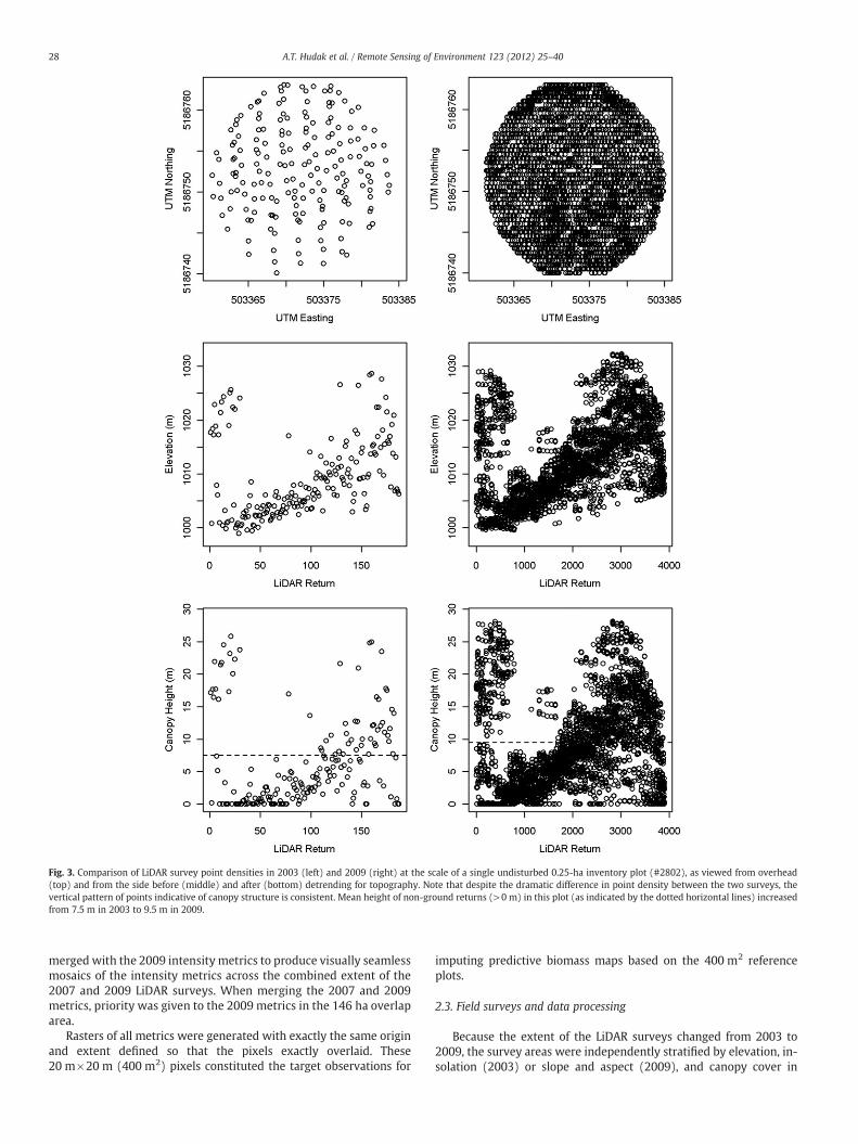
Fig. 3. Comparison of LiDAR survey point densities in 2003 (left) and 2009 (right) at the scale of a single undisturbed 0.25-ha inventory plot (#2802), as viewed from overhead(top) and from the side before (middle) and after (bottom) detrending for topography. Note that despite the dramatic difference in point density between the two surveys, thevertical pattern of points indicative of canopy structure is consistent. Mean height of non-ground returns (>0 m) in this plot (as indicated by the dotted horizontal lines) increasedfrom 7.5 m in 2003 to 9.5 m in 2009.

28 A.T. Hudak et al. / Remote Sensing of Environment 123 (2012) 25–40

merged with the 2009 intensity metrics to produce visually seamlessmosaics of the intensity metrics across the combined extent of the2007 and 2009 LiDAR surveys. When merging the 2007 and 2009metrics, priority was given to the 2009 metrics in the 146 ha overlaparea.

Rasters of all metrics were generated with exactly the same originand extent defined so that the pixels exactly overlaid. These20 m×20 m (400 m2) pixels constituted the target observations for

imputing predictive biomass maps based on the 400 m2 referenceplots.

2.3. Field surveys and data processing

Because the extent of the LiDAR surveys changed from 2003 to2009, the survey areas were independently stratified by elevation, in-solation (2003) or slope and aspect (2009), and canopy cover in

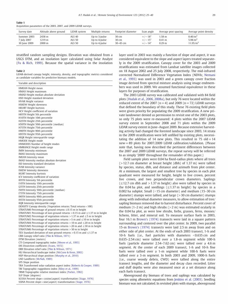
Table 1Acquisition parameters of the 2003, 2007, and 2009 LiDAR surveys.

Survey date Altitude above ground LiDAR system Multiple returns Footprint diameter Scan angle Average post spacing Average point density

Summer 2003 2438 m ALS 40 Up to 3/pulse 30 cm +/−18° 1.58 m 0.40/m2

7 July 2007 1219 m ALS 50 Up to 4/pulse 30 cm +/−15° 0.41 m 5.98/m2

30 June 2009 2000 m ALS 50 Up to 4/pulse 30–45 cm +/−14° 0.29 m 11.95/m2

29A.T. Hudak et al. / Remote Sensing of Environment 123 (2012) 25–40

stratified random sampling designs. Elevation was obtained from aUSGS DTM, and an insolation layer calculated using Solar Analyst(Fu & Rich, 1999). Because the spatial variance in the insolation

Table 2LiDAR-derived canopy height, intensity, density, and topographic metrics consideredas candidate variables for predictive biomass models.

Variable and description

HMEAN Height meanHMAX Height maximumHMAD Height median absolute deviationHSD Height standard deviationHVAR Height varianceHSKEW Height skewnessHKURT Height kurtosisHCV Height coefficient of variationH05TH Height 5th percentileH10TH Height 10th percentileH25TH Height 25th percentileH50TH Height 50th percentile (median)H75TH Height 75th percentileH90TH Height 90th percentileH95TH Height 95th percentileHIQR Height interquartile rangeHMODE Height modeHNMODES Number of height modesHMRANGE Height mode rangeIMIN Intensity minimumIMAX Intensity maximumIMEAN Intensity meanIMAD Intensity median absolute deviationISD Intensity standard deviationIVAR Intensity varianceISKEW Intensity skewnessIKURT Intensity kurtosisICV Intensity coefficient of variationI05TH Intensity 5th percentileI10TH Intensity 10th percentileI25TH Intensity 25th percentileI50TH Intensity 50th percentile (median)I75TH Intensity 75th percentileI90TH Intensity 90th percentileI95TH Intensity 95th percentileIIQR Intensity interquartile rangeDENSITY Canopy density (Vegetation returns /Total returns×100)STRATUM0 Percentage of ground returns ≤0.15 m in heightSTRATUM1 Percentage of non-ground returns >0.15 m and ≤1.37 m in heightSTRATUM2 Percentage of vegetation returns >1.37 m and ≤5 m in heightSTRATUM3 Percentage of vegetation returns >5 m and ≤10 m in heightSTRATUM4 Percentage of vegetation returns >10 m and ≤20 m in heightSTRATUM5 Percentage of vegetation returns >20 m and ≤30 m in heightSTRATUM6 Percentage of vegetation returns >30 m in heightTEX Standard deviation of non-ground returns >0.15 m and ≤1.37 mCRR Canopy relief ratio (Pike & Wilson, 1971)DTM Elevation (meters)CTI Compound topographic index (Moore et al., 1993)DIS Dissection coefficient (Evans, 1972)ERR Elevation relief ratio (Pike & Wilson, 1971)HLI Hierarchical landscape index (McCune & Keon, 2002)HSP Hierarchical slope position (Murphy et al., 2010)LND Landform (McNab, 1989)SPS Slope positionTRA Transformed solar-radiation aspect index (Roberts & Cooper, 1989)TRI Topographic ruggedness index (Riley et al., 1999)TRMI Topographic relative moisture index (Parker, 1982)SLP Slope (degrees)SCOSA Percent slope×cosine(aspect) transformation (Stage, 1976)SSINA Percent slope×sine(aspect) transformation (Stage, 1976)

layer used in 2003 was mainly a function of slope and aspect, it wasconsidered equivalent to the slope and aspect layers treated separate-ly in the 2009 stratification. Canopy cover for the 2003 and 2009stratifications was estimated from Landsat satellite images collectedon 18 August 2002 and 25 July 2008, respectively. The mid-infraredcorrected Normalized Difference Vegetation Index (NDVIc, Nemaniet al., 1993) was used in 2003 and a green canopy cover fractionimage derived from spectral mixture analysis using image endmem-bers was used in 2009. We assumed functional equivalence in theselayers for purposes of stratification.

The 2003 LiDAR survey was calibrated and validated with 84 fieldplots (Hudak et al., 2006, 2008a), but only 76 were located within thereduced extent of the 2007 (n=4) and 2009 (n=72) LiDAR surveysthat defined the boundary of this study. These 76 existing field plotswere given priority for populating the 2009 stratification. A new pri-vate landowner denied us permission to revisit one of the 2003 plots,so only 75 plots were re-measured: 4 plots within the 2007 LiDARsurvey extent in September 2008 and 71 plots within the 2009LiDAR survey extent in June–August 2009. Because extensive harvest-ing activity had changed the forested landscape since 2003, 14 stratain the 2009 stratification were left unfilled by existing plots, necessi-tating the addition of 14 new plots. This resulted in 75 old+14new=89 plots for 2007/2009 LiDAR calibration/validation. (Pleasenote that, having now described the pertinent differences betweenthe 2007 and 2009 LiDAR surveys, the repeat survey will be referredto as simply ‘2009’ throughout the remainder of this paper.)

Field sample plots were 0.04 ha fixed-radius plots where all trees(>12.7 cm diameter at breast height (dbh) of 1.37 m) were talliedby species, status, dbh, and distance and azimuth from plot center.At a minimum, the largest and smallest tree by species in each plotquadrant were measured for height, height to live crown, percentlive crown, and two perpendicular crown diameters. Saplings(≤12.7 cm dbh and >1.37 m height) also were tallied by species inthe 0.04 ha plot, and seedlings (≤1.37 m height) by species in a0.002 ha subplot. Small (b15 cm diameter) and medium (15–30 cmdiameter) stumps were tallied, and large (>30 cm diameter) stumpsalong with individual diameter measures, to allow estimation of tree/sapling biomass removed due to harvest disturbance. Percent cover ofmedium (1–2 m) and high shrubs (>2 m) was estimated ocularly inthe 0.04 ha plot, as were low shrubs, forbs, grasses, ferns, mosses/lichens, litter, and mineral soil. To measure surface fuels in 2003,four 16.1 m Brown's (1974) transects were laid in a square patternsurrounding and centered over the plot center. In 2009, two parallel15-m Brown's (1974) transects were laid 2.5 m away from and oneither side of plot center. At the ends of each 2003 transect, 1-h and10-h fuels (i.e., fuel particles with diameters b0.635 cm and0.635–2.54 cm) were tallied over a 1.8-m segment while 100-hfuels (particle diameter 2.54–7.62 cm) were tallied over a 4.6 msegment. At the center of each 2009 transect, 1-h and 10-h finefuels were tallied over a 1-m segment while 100-h fuels weretallied over a 3-m segment. In both 2003 and 2009, 1000-h fuels(i.e., coarse woody debris, CWD) were tallied along the entiretransect lengths, and the diameter and decay class recorded. Litterand duff depths were also measured once at a set distance alongeach fuels transect.

Aboveground dry biomass of trees and saplings was calculated byspecies using allometric equations from Jenkins et al. (2003). Seedlingbiomass was not calculated. In revisited plots with stumps, aboveground

30 A.T. Hudak et al. / Remote Sensing of Environment 123 (2012) 25–40

dry biomass removed from sitewas calculated from the stumpdiametermeasurements, using a biomass equation generalized from Jenkins et al.(2003) across the mix of species represented in the study area. Thestump diameters were downsized by a factor of 0.9 to account for thetaper between the height of the stumps and breast height (Bones,1960). Shrub and herbaceous biomasses were estimated from the per-cent covermeasures following Smith and Brand (1983)whileweightingthe low, medium, and high shrub classes by their midpoint diameters of0.5, 1.5, and 2.5 cm, respectively. Percent cover measures of forbs,grasses, ferns, and mosses/lichens were averaged and converted to bio-mass following Brown (1981), with a bulk density of 1.9 kg/m3 for agrass-shrub type fuelbed with a midpoint depth of 0.25 m in habitattype P. menziesii (Mirb.) Franco/Physocarpus malvaceus (Greene) Kuntzh.t.—P. malvaceus phase (PSME/PHMA). Surface fuels were sampledwith twice the effort in 2003 than in 2009, but the different downedwoody debris (DWD) transect lengthswere accounted for in the volumeequation of Harmon and Sexton (1996) using improved midpoint qua-dratic mean diameters (QMD) for the three fine woody debris (FWD)classes obtained from Woodall and Monleon (2006). DWD volumeswere converted to biomass using density coefficients from Brown(1974). Litter and duff biomasses were estimated from the litterand duff depth measures following Brown et al. (1981), using aspecific gravity of 25.3 kg/m3 for PSME/PHMA litter (Brown, 1981)and a specific gravity of 110.5 kg/m3 for mixed conifer forest duff(Wooldridge, 1968).

Biomass calculated for the various tree and non-tree pools wasconverted to carbon loads using carbon concentrations from Jain etal. (2010), which ranged from 0.379 (litter and duff) to 0.495 (treeboles). Whole tree biomass pools were multiplied by ratios of 0.8and 0.2 to convert the boles and crowns to carbon, respectively,because the reported carbon concentrations differed. All of theaboveground carbon pools were then summed to calculate totalcarbon.

LiDAR canopy metrics were also computed within each 11.35 mradius inventory plot, and the topographic metrics were extractedfrom the 20 m topographic layers at each plot center. These 0.04 ha(400 m2) plot-level metrics constituted the reference observationsfor developing predictive biomass models. Note that the model andmap units were the same 400 m2 size to preclude scale effects.

2.4. Predictive biomass modeling

The Random Forest (RF) algorithm applied in this study for impu-tation was called from the yaImpute package (Crookston & Finley,2008) in R (R Development Team, v2.10.0). Random Forest is a non-parametric technique that can handle both continuous and categori-cal independent variables and can be run in either regression modeor classification mode. The RF technique uses a bootstrap approachfor achieving higher accuracies compared to traditional classificationtrees. RF uses the Gini statistic for node splitting which allows fornon-linear variable interactions. A large number of classificationtrees are produced, permutations are introduced at each node, andthe most common classification result is selected.

Our predictive modeling strategy was to treat each time period asan independent assessment, as a forest manager is likely to do. The2003 and 2009 biomass models were therefore developed separatelybased on all available contemporaneous plot measures from either2003 (n=76) or 2009 (n=89). Variable selection from the suite of62 candidate LiDAR height, intensity, density, and topographic metrics(Table 2) was performed separately yet consistently. We ran a RandomForest model selection function that uses Model Improvement Ratio(MIR) standardized importance values (Evans & Cushman, 2009;Evans et al., 2010; Murphy et al., 2010) to objectively choose themost important LiDAR metrics for predicting the response variables. Ifselected predictor variables were highly correlated (Pearson's r>0.9),we excluded from consideration the variable with lesser importance

according to the MIR statistic, and we repeated the model selectionfunction to search for alternative predictors. In the interest of parsimo-ny, a subset of influential predictors was further reduced to the tenLiDAR metrics having the greatest importance.

Following the strategy of Hudak et al. (2008a) to assign moreweight to the more prevalent tree species, the three response vari-ables included in the imputation model were total tree biomass, thebiomass of the dominant species in each inventory plot, and thename of the dominant species in each inventory plot. By includingtree species as a response, we could impute species-level tree bio-mass and not simply total tree biomass (Hudak et al., 2008a). Anotheradvantage of imputation, besides the ability to simultaneously predictmultiple responses, is that not all response variables need to beincluded in the neighborhood calculations to predict them. Forinstance in this study, we did not include the non-tree biomass orcarbon pool variables in the neighborhood calculations, but imputedthem nonetheless through their plot-level association to treebiomass; i.e., the understory live biomass pools were imputed as an-cillary variables: saplings, shrubs, and herbaceous vegetation; aswere the decomposing biomass pools: coarse and fine woody debris,litter, and duff. We also imputed habitat type (Cooper et al., 1991);the majority habitat type imputed to the map cells within eachstand was used to parameterize the Forest Vegetation Simulator(FVS) projections of tree biomass from stand-level cruise data collect-ed across the Moscow Mountain and used in this study for indepen-dent validation.

2.5. Biomass/carbon change estimation and validation

Plot-level tree biomass was imputed to the 400 m2 reference plotsfor model validation using the root mean square difference (RMSD)and Pearson correlation statistics. The RMSD used to assess imputa-tion model accuracy (Stage & Crookston, 2007) is analogous to theRMSE used to assess regressionmodel accuracy. The RMSD is typicallylarger than the RMSE because imputed predictions preserve the vari-ance in the observations, while regression predictions have reducedvariance relative to observations. Indeed, regression predictions areunique values that can be plotted along a line, whereas imputed pre-dictions are observations themselves. Thus, the imputed value at eachplot represents the total tree biomass observed at its nearest neighborplot (in terms of multivariate statistical distance). Predictions werealso imputed to the 400 m2 target cells defined by the grids of theten LiDAR metrics included in the 2003 and 2009 models. Since thenumber of reference observations (i.e., plots) was so small relativeto the number of target observations (i.e., individual grid cells), a sys-tematic sample of grid cell predictor and response variables wereextracted from the maps at 500 m intervals to compare the distribu-tion of grid cell values across the landscape to the distribution ofplot values designed to represent the landscape.

Fluxes of biomass and carbon were calculated over the six yeartime period by subtracting the 2003 maps of biomass/carbon poolsfrom those of 2009. Positive values thus indicate net biomass/carbongain while negative values indicate loss. Biomass change results weresummarized in tabular format for harvested and non-harvested for-ested areas and non-forest. Non-forest was classified as areas with aDENSITY metric of zero in both 2003 and 2009; i.e., no LiDAR returnshigher than breast height (1.37 m) within the 20 m×20 m pixel.Biomass change within structural stages was estimated via overlayanalysis between a map of structural stages developed for the samestudy area by Falkowski et al. (2009) and the change in total biomassestimated as part of this project. Structural stages mapped byFalkowski et al. (2009) followed a classification scheme developedby O'Hara et al. (1996) and included: Open—treeless areas (9 plots);Stand Initiation (si)—space reoccupied by seedlings, saplings orshrubs following a stand replacing disturbance (7 plots); UnderstoryReinitiation (ur)—older cohort of trees being replaced by new

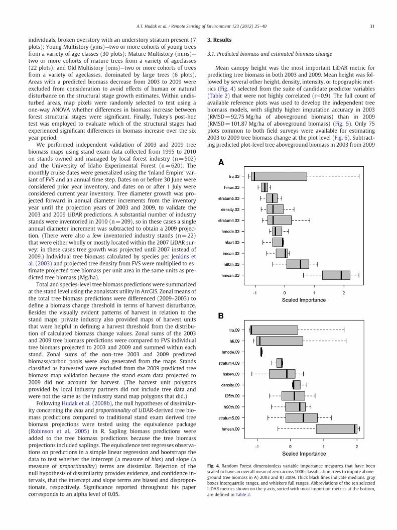
Fig. 4. Random Forest dimensionless variable importance measures that have beenscaled to have an overall mean of zero across 1000 classification trees to impute above-ground tree biomass in A) 2003 and B) 2009. Thick black lines indicate medians, grayboxes interquartile ranges, and whiskers full ranges. Abbreviations of the ten selectedLiDAR metrics shown on the y axis, sorted with most important metrics at the bottom,are defined in Table 2.

31A.T. Hudak et al. / Remote Sensing of Environment 123 (2012) 25–40

individuals, broken overstory with an understory stratum present (7plots); Young Multistory (yms)—two or more cohorts of young treesfrom a variety of age classes (30 plots); Mature Multistory (mms)—two or more cohorts of mature trees from a variety of ageclasses(22 plots); and Old Multistory (oms)—two or more cohorts of treesfrom a variety of ageclasses, dominated by large trees (6 plots).Areas with a predicted biomass decrease from 2003 to 2009 wereexcluded from consideration to avoid effects of human or naturaldisturbance on the structural stage growth estimates. Within undis-turbed areas, map pixels were randomly selected to test using aone-way ANOVA whether differences in biomass increase betweenforest structural stages were significant. Finally, Tukey's post-hoctest was employed to evaluate which of the structural stages hadexperienced significant differences in biomass increase over the sixyear period.

We performed independent validation of 2003 and 2009 treebiomass maps using stand exam data collected from 1995 to 2010on stands owned and managed by local forest industry (n=502)and the University of Idaho Experimental Forest (n=620). Themonthly cruise dates were generalized using the ‘Inland Empire’ var-iant of FVS and an annual time step. Dates on or before 30 June wereconsidered prior year inventory, and dates on or after 1 July wereconsidered current year inventory. Tree diameter growth was pro-jected forward in annual diameter increments from the inventoryyear until the projection years of 2003 and 2009, to validate the2003 and 2009 LiDAR predictions. A substantial number of industrystands were inventoried in 2010 (n=209), so in these cases a singleannual diameter increment was subtracted to obtain a 2009 projec-tion. (There were also a few inventoried industry stands (n=22)that were either wholly or mostly located within the 2007 LiDAR sur-vey; in these cases tree growth was projected until 2007 instead of2009.) Individual tree biomass calculated by species per Jenkins etal. (2003) and projected tree density from FVS were multiplied to es-timate projected tree biomass per unit area in the same units as pre-dicted tree biomass (Mg/ha).

Total and species-level tree biomass predictions were summarizedat the stand level using the zonalstats utility in ArcGIS. Zonal means ofthe total tree biomass predictions were differenced (2009–2003) todefine a biomass change threshold in terms of harvest disturbance.Besides the visually evident patterns of harvest in relation to thestand maps, private industry also provided maps of harvest unitsthat were helpful in defining a harvest threshold from the distribu-tion of calculated biomass change values. Zonal sums of the 2003and 2009 tree biomass predictions were compared to FVS individualtree biomass projected to 2003 and 2009 and summed within eachstand. Zonal sums of the non-tree 2003 and 2009 predictedbiomass/carbon pools were also generated from the maps. Standsclassified as harvested were excluded from the 2009 predicted treebiomass map validation because the stand exam data projected to2009 did not account for harvest. (The harvest unit polygonsprovided by local industry partners did not include tree data andwere not the same as the industry stand map polygons that did.)

Following Hudak et al. (2008b), the null hypotheses of dissimilar-ity concerning the bias and proportionality of LiDAR-derived tree bio-mass predictions compared to traditional stand exam derived treebiomass projections were tested using the equivalence package(Robinson et al., 2005) in R. Sapling biomass predictions wereadded to the tree biomass predictions because the tree biomassprojections included saplings. The equivalence test regresses observa-tions on predictions in a simple linear regression and bootstraps thedata to test whether the intercept (a measure of bias) and slope (ameasure of proportionality) terms are dissimilar. Rejection of thenull hypothesis of dissimilarity provides evidence, and confidence in-tervals, that the intercept and slope terms are biased and dispropor-tionate, respectively. Significance reported throughout his papercorresponds to an alpha level of 0.05.

3. Results

3.1. Predicted biomass and estimated biomass change

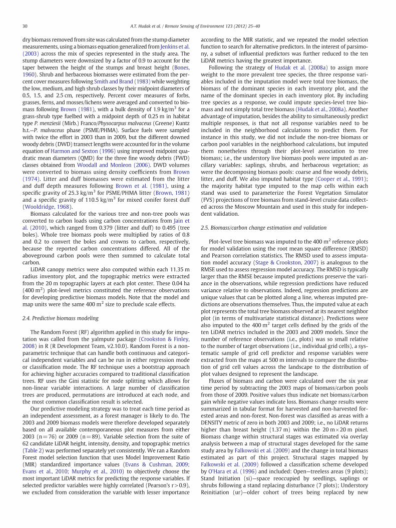
Mean canopy height was the most important LiDAR metric forpredicting tree biomass in both 2003 and 2009. Mean height was fol-lowed by several other height, density, intensity, or topographic met-rics (Fig. 4) selected from the suite of candidate predictor variables(Table 2) that were not highly correlated (rb0.9). The full count ofavailable reference plots was used to develop the independent treebiomass models, with slightly higher imputation accuracy in 2003(RMSD=92.75 Mg/ha of aboveground biomass) than in 2009(RMSD=101.87 Mg/ha of aboveground biomass) (Fig. 5). Only 75plots common to both field surveys were available for estimating2003 to 2009 tree biomass change at the plot level (Fig. 6). Subtract-ing predicted plot-level tree aboveground biomass in 2003 from 2009

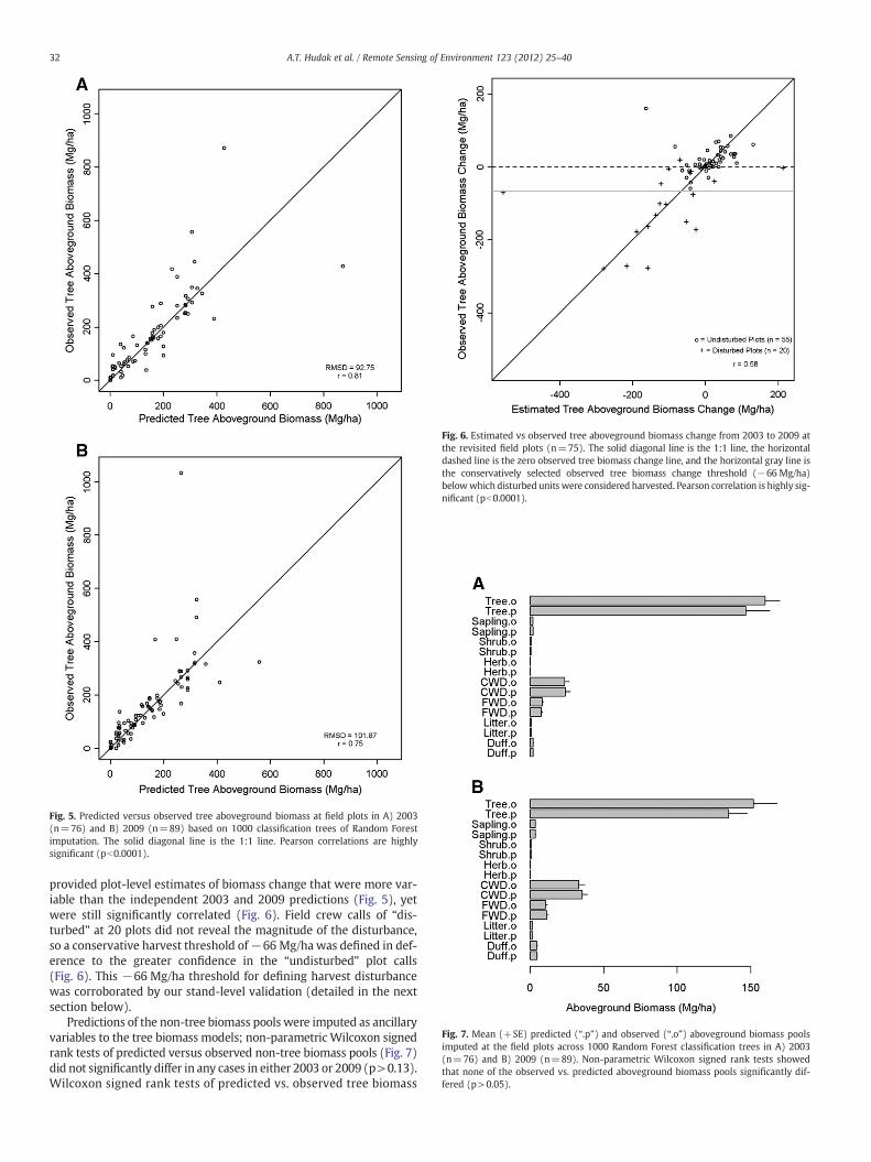
Fig. 5. Predicted versus observed tree aboveground biomass at field plots in A) 2003(n=76) and B) 2009 (n=89) based on 1000 classification trees of Random Forestimputation. The solid diagonal line is the 1:1 line. Pearson correlations are highlysignificant (pb0.0001).

Fig. 6. Estimated vs observed tree aboveground biomass change from 2003 to 2009 atthe revisited field plots (n=75). The solid diagonal line is the 1:1 line, the horizontaldashed line is the zero observed tree biomass change line, and the horizontal gray line isthe conservatively selected observed tree biomass change threshold (−66 Mg/ha)belowwhich disturbed units were considered harvested. Pearson correlation is highly sig-nificant (pb0.0001).

Fig. 7. Mean (+SE) predicted (“.p”) and observed (“.o”) aboveground biomass poolsimputed at the field plots across 1000 Random Forest classification trees in A) 2003(n=76) and B) 2009 (n=89). Non-parametric Wilcoxon signed rank tests showedthat none of the observed vs. predicted aboveground biomass pools significantly dif-fered (p>0.05).

32 A.T. Hudak et al. / Remote Sensing of Environment 123 (2012) 25–40

provided plot-level estimates of biomass change that were more var-iable than the independent 2003 and 2009 predictions (Fig. 5), yetwere still significantly correlated (Fig. 6). Field crew calls of “dis-turbed” at 20 plots did not reveal the magnitude of the disturbance,so a conservative harvest threshold of−66 Mg/ha was defined in def-erence to the greater confidence in the “undisturbed” plot calls(Fig. 6). This −66 Mg/ha threshold for defining harvest disturbancewas corroborated by our stand-level validation (detailed in the nextsection below).

Predictions of the non-tree biomass pools were imputed as ancillaryvariables to the tree biomass models; non-parametric Wilcoxon signedrank tests of predicted versus observed non-tree biomass pools (Fig. 7)did not significantly differ in any cases in either 2003 or 2009 (p>0.13).Wilcoxon signed rank tests of predicted vs. observed tree biomass

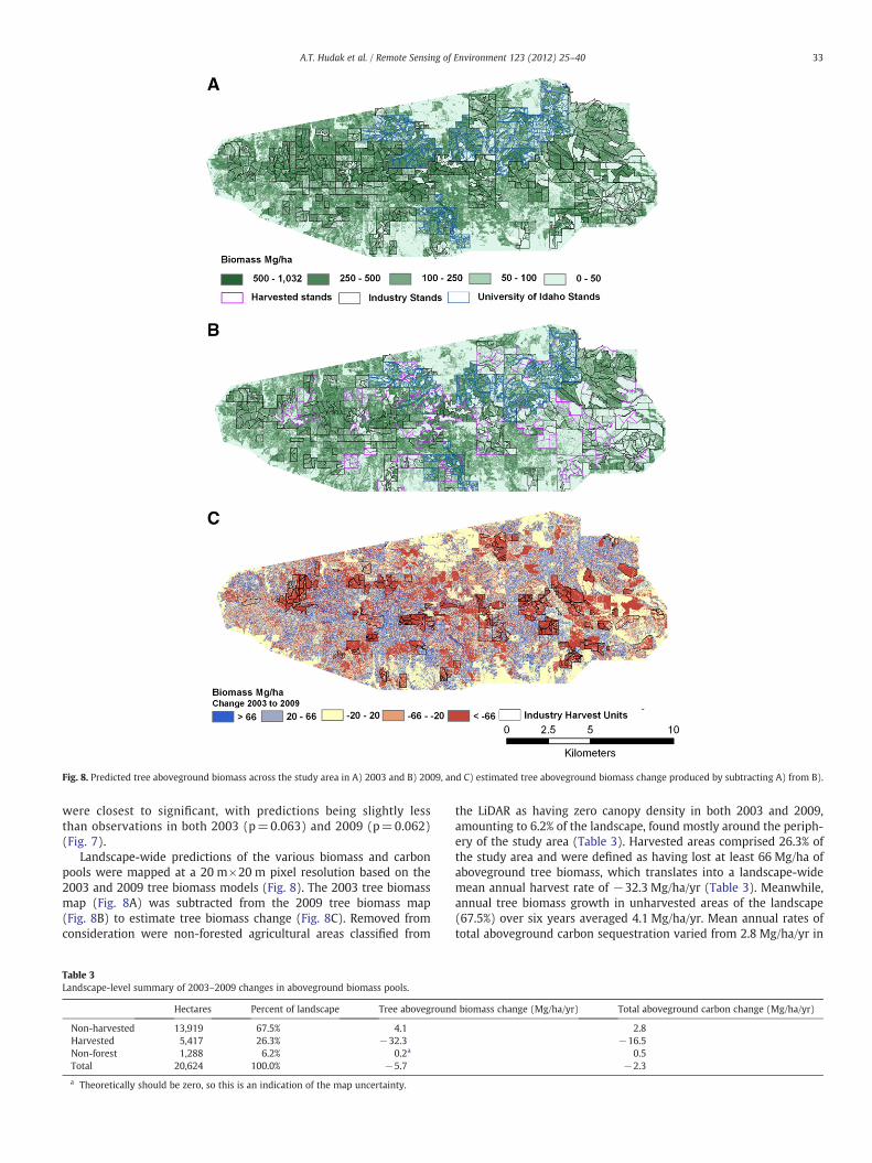
Fig. 8. Predicted tree aboveground biomass across the study area in A) 2003 and B) 2009, and C) estimated tree aboveground biomass change produced by subtracting A) from B).

33A.T. Hudak et al. / Remote Sensing of Environment 123 (2012) 25–40

were closest to significant, with predictions being slightly lessthan observations in both 2003 (p=0.063) and 2009 (p=0.062)(Fig. 7).

Landscape-wide predictions of the various biomass and carbonpools were mapped at a 20 m×20 m pixel resolution based on the2003 and 2009 tree biomass models (Fig. 8). The 2003 tree biomassmap (Fig. 8A) was subtracted from the 2009 tree biomass map(Fig. 8B) to estimate tree biomass change (Fig. 8C). Removed fromconsideration were non-forested agricultural areas classified from

Table 3Landscape-level summary of 2003–2009 changes in aboveground biomass pools.

Hectares Percent of landscape Tree aboveground

Non-harvested 13,919 67.5% 4.1Harvested 5,417 26.3% −32.3Non-forest 1,288 6.2% 0.2a

Total 20,624 100.0% −5.7

a Theoretically should be zero, so this is an indication of the map uncertainty.

the LiDAR as having zero canopy density in both 2003 and 2009,amounting to 6.2% of the landscape, found mostly around the periph-ery of the study area (Table 3). Harvested areas comprised 26.3% ofthe study area and were defined as having lost at least 66 Mg/ha ofaboveground tree biomass, which translates into a landscape-widemean annual harvest rate of −32.3 Mg/ha/yr (Table 3). Meanwhile,annual tree biomass growth in unharvested areas of the landscape(67.5%) over six years averaged 4.1 Mg/ha/yr. Mean annual rates oftotal aboveground carbon sequestration varied from 2.8 Mg/ha/yr in

biomass change (Mg/ha/yr) Total aboveground carbon change (Mg/ha/yr)

2.8−16.5

0.5−2.3

34 A.T. Hudak et al. / Remote Sensing of Environment 123 (2012) 25–40

unharvested lands to −16.5 Mg/ha/yr in harvested lands, or−2.3 Mg/ha/yr overall; thus, the intensive and extensive harvest ac-tivities across the Moscow Mountain study area resulted in an overallloss in aboveground carbon from the landscape over the 6-year studyperiod (Table 3).

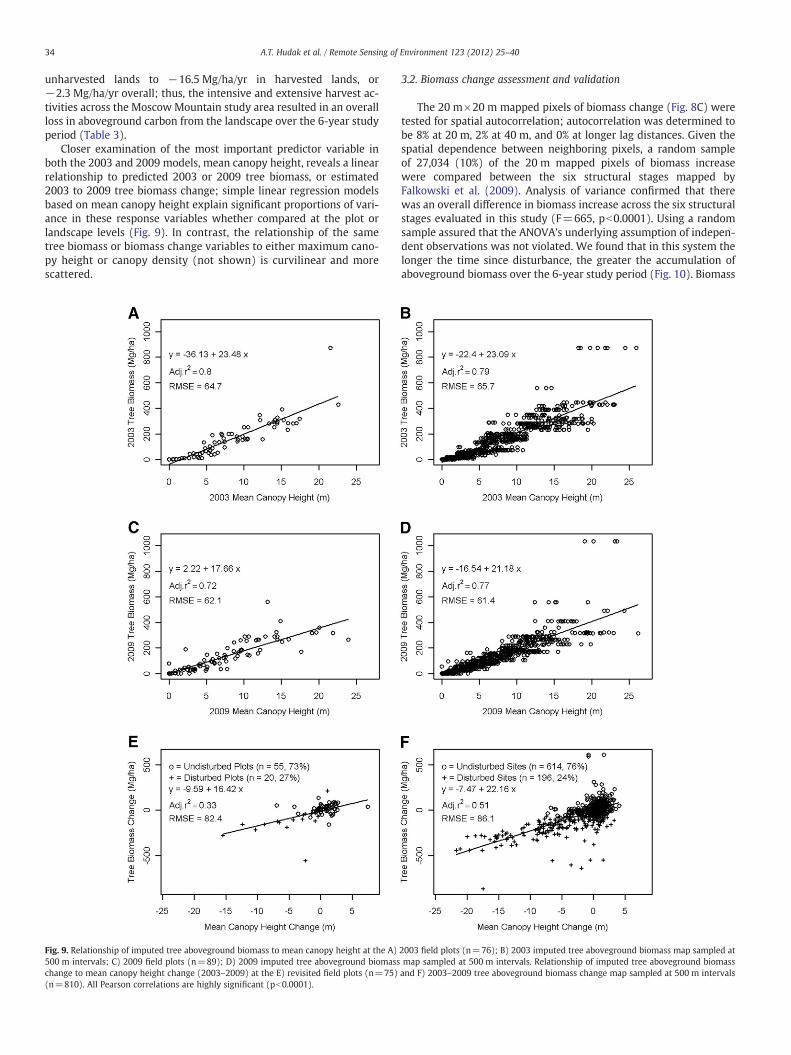
Closer examination of the most important predictor variable inboth the 2003 and 2009 models, mean canopy height, reveals a linearrelationship to predicted 2003 or 2009 tree biomass, or estimated2003 to 2009 tree biomass change; simple linear regression modelsbased on mean canopy height explain significant proportions of vari-ance in these response variables whether compared at the plot orlandscape levels (Fig. 9). In contrast, the relationship of the sametree biomass or biomass change variables to either maximum cano-py height or canopy density (not shown) is curvilinear and morescattered.

Fig. 9. Relationship of imputed tree aboveground biomass to mean canopy height at the A)500 m intervals; C) 2009 field plots (n=89); D) 2009 imputed tree aboveground biomasschange to mean canopy height change (2003–2009) at the E) revisited field plots (n=75)(n=810). All Pearson correlations are highly significant (pb0.0001).

3.2. Biomass change assessment and validation

The 20 m×20 m mapped pixels of biomass change (Fig. 8C) weretested for spatial autocorrelation; autocorrelation was determined tobe 8% at 20 m, 2% at 40 m, and 0% at longer lag distances. Given thespatial dependence between neighboring pixels, a random sampleof 27,034 (10%) of the 20 m mapped pixels of biomass increasewere compared between the six structural stages mapped byFalkowski et al. (2009). Analysis of variance confirmed that therewas an overall difference in biomass increase across the six structuralstages evaluated in this study (F=665, pb0.0001). Using a randomsample assured that the ANOVA's underlying assumption of indepen-dent observations was not violated. We found that in this system thelonger the time since disturbance, the greater the accumulation ofaboveground biomass over the 6-year study period (Fig. 10). Biomass

2003 field plots (n=76); B) 2003 imputed tree aboveground biomass map sampled atmap sampled at 500 m intervals. Relationship of imputed tree aboveground biomassand F) 2003–2009 tree aboveground biomass change map sampled at 500 m intervals

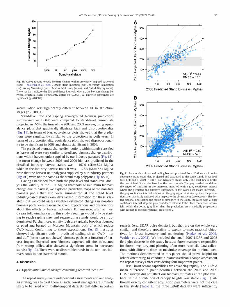
Fig. 10. Above ground woody biomass change within previously mapped structuralstages (Falkowski et al., 2009). Open; Stand Initiation (si); Understory Reinitiation(ur); Young Multistory (yms); Mature Multistory (mms); and Old Multistory (oms).The error bars indicate the 95% confidence intervals. Overall, the biomass change be-tween structural stages significantly differs (pb0.0001). All pairwise differences aresignificant (pb0.0001).

Fig. 11. Relationship of tree and sapling biomass predicted from LiDAR versus from in-dependent stand exam data projected and expanded to the same stands in A) 2003(n=174) and B) 2009 (n=881, non-harvested stands only). The black line indicatesthe line of best fit and the blue line the loess smooth. The gray shaded bar definesthe region of similarity in the intercept, indicated with a gray confidence intervalwhere the predicted and observed (projected, in this case) data means intersect. Ifthe gray confidence interval falls within the gray region of similarity, then the predic-tions are statistically unbiased with respect to the observations (projections). The dot-ted diagonal lines define the region of similarity in the slope, indicated with a blackconfidence interval atop the gray confidence interval. If the black confidence intervalfalls within the dotted gray lines, then the predictions are statistically proportionalwith respect to the observations (projections).

35A.T. Hudak et al. / Remote Sensing of Environment 123 (2012) 25–40

accumulation was significantly different between all six structuralstages (pb0.0001).

Stand-level tree and sapling aboveground biomass predictionssummarized via LiDAR were compared to stand-level cruise dataprojected in FVS to the time of the 2003 and 2009 surveys, using equiv-alence plots that graphically illustrate bias and disproportionality(Fig. 11). In terms of bias, equivalence plots showed that the predic-tions were significantly similar to the projections in both years. Interms of disproportionality, equivalence plots showed disproportional-ity to be significant in 2003 and almost significant in 2009.

The predicted biomass change distributions within stands classifiedas harvested were very similar to predicted biomass change distribu-tions within harvest units supplied by our industry partners (Fig. 12);the mean change between 2003 and 2009 biomass predicted in theclassified industry harvest stands was −167.0 (SE=5.2) Mg/ha,while in the industry harvest units it was −173.3 (SE=7.8) Mg/ha.Note that the harvest unit polygons supplied by our industry partners(Fig. 8C) were not the same as the stand map polygons (Fig. 8A, B).

Having established from both the plot-level and stand-level anal-ysis the validity of the −66 Mg/ha threshold of minimum biomasschange due to harvest, we explored predictive maps of the non-treebiomass pools that also were summarized at the stand level.Industry-based stand exam data lacked information for these vari-ables, but we could assess whether estimated changes in non-treebiomass pools were reasonable given expectations and observationsabout the effects of harvest activities. For instance, after at most6 years following harvest in this study, seedlings would only be start-ing to reach sapling size, and regenerating stands would be shrub-dominated. Furthermore, activity fuels are typically broadcast burnedor piled and burned on Moscow Mountain, both of which reduceCWD loads. Conforming to these expectations, Fig. 13 illustratesobserved significant trends in predicted sapling, shrub, CWD, litterand duff (latter two not shown) biomass pools as a function of har-vest impact. Expected tree biomass exported off site, calculatedfrom stump tallies, also showed a significant trend in harvestedstands (Fig. 13). There were no discernible trends in the non-tree bio-mass pools in non-harvested stands.

4. Discussion

4.1. Opportunities and challenges concerning repeated measures

The repeat surveys were independent assessments and our analy-sis strategy was to treat them as such. Forest managers are similarlylikely to be faced with multi-temporal datasets that differ in certain

regards (e.g., LiDAR pulse density), but that are on the whole verysimilar, and therefore appealing to exploit to meet practical objec-tives for forest inventory and monitoring (Hudak et al., 2009;Wulder et al., 2008). We included the small 2007 LiDAR and 2008field plot datasets in this study because forest managers responsiblefor forest inventory and planning often must reconcile data collec-tions with different dates to maximize coverage for minimal cost.The methods demonstrated in this paper should prove helpful forothers attempting to conduct a biomass/carbon change assessmentvia repeat surveys after considering four important points.

First, LiDAR sensor capabilities are advancing rapidly. The 30-foldmean difference in point densities between the 2003 and 2009LiDAR surveys did not affect our biomass estimates at the plot level,because the distribution of canopy heights was stable (Fig. 3). Al-though exactly consistent acquisition parameters were not the casein this study (Table 1), the three LiDAR datasets were sufficiently

Fig. 12. Relationship of imputed tree aboveground biomass in 2003 and 2009 inA) stands classified as non-harvested or harvested (Fig. 8B) compared toB) 2003–2009 industry harvest units (Fig. 8C); i.e., industry harvest units in B) arenot the same as harvested stands in A).

36 A.T. Hudak et al. / Remote Sensing of Environment 123 (2012) 25–40

comparable when aggregated to the 400 m2 scale. The 0.4 points/m2

mean point density of the 2003 survey translates to a mean of160 points per 0.25-ha (400 m2) plot, which is a sufficient numberof points to produce a stable canopy height distribution from whichto calculate canopy height metrics. Maximum canopy height maybe a less reliable metric to compare between repeat LiDAR surveys;for instance, the higher LiDAR pulse density in 2009 compared to2003 would translate into less height underestimation bias in 2009than in 2003, whereas mean canopy height would be less subjectto such a bias. The mean of 4790 points per plot collected in 2009represents over-sampling at the plot level of aggregation. Such highdensity LiDAR can permit individual tree characterization underopen canopy conditions but not easily or accurately in closedcanopies like on much of Moscow Mountain (Falkowski et al., 2006,2008).

Second, it is important that the calibration/validation plots repre-sent forest conditions across the landscape in a representative andunbiased manner. The repeat LiDAR coverage was of smaller extentthan the 2003 LiDAR coverage, affecting the landscape stratification.Six of the eight 2003 plots located exterior to the repeat LiDAR sur-veys were non-forested plots, making their exclusion from the 2003model inconsequential. However, the high degree of change due toharvest activity within the study landscape required the addition of

14 new plots to populate the re-stratification. Our results supportthe idea that forest inventory plots used to develop predictive bio-mass models need not be exactly the same to produce comparable re-sults between repeat inventories. Representative sampling can beaccomplished through random or random stratified sampling designsconditioned on the spatial extent of the landscape they represent, orsystematic monitoring plots as used by the USFS Forest Inventoryand Analysis program (FIA). The coarse spatial frequency of FIAplots relative to this and most other LiDAR project areas requiresmore intensive localized sampling to adequately characterize therange of variability in forest structure conditions. Upscaling of plot-level biomass data into wall-to-wall maps as demonstrated by thisstudy could be replicated at regional or even national scales usingFIA plot data as broader LiDAR coverage becomes available (Stokeret al., 2008; Vierling et al., 2011). Such LiDAR data products neednot necessarily be spatially contiguous but could be developed via in-tegration between distributed LiDAR sample data and contiguousLandsat or other satellite imagery (Hudak et al., 2002).

Third, our inventory plots were not originally established for high-precision repeat monitoring. Although 75 of the field plots estab-lished in 2003 were re-measured in 2009, they had not been markedwith permanent monuments in 2003. The 2009 field crews navigatedto and placed the 2009 plot centers as closely as possible to theunmarked 2003 plot center locations. Despite the fact that both the2003 and 2009 plot centers were geolocated with differential GPS,differences between 2003 and 2009 plot locations vary from 0.46 mto 9.25 m with a mean of 2.67 m and a standard deviation of 1.65 m.These offsets do not include the additive uncertainties in the 2003and 2009 plot locations. We expected the geolocation errors to con-tribute greatly to the scatter in the biomass change estimates illus-trated in Fig. 6. However, when we tested the effect of thegeolocation offsets on overall error in estimated biomass change inthe 55 non-harvested plots, by regressing 2009 biomass observationson 2003 biomass observations in a simple linear regression model(y=1.07x+9.39, RMSE=32.7 Mg/ha, Adj. r2=0.96, pb0.0001) andthen comparing the residuals against the offsets calculated betweenthe 2003 and 2009 recorded plot center locations, we found no rela-tionship (r=−0.01, p=0.94). This suggests that 2003 and 2009 im-putation model errors and pure error (Stage & Crookston, 2007) maybe larger contributors to the overall errors in predicted biomass thaninconsistencies in plot location between the field sampling periods.These additive errors are cumulative when summed across repeatedmeasurements, and should contribute to higher variance in biomasschange predictions than biomass predictions confined to a singletime. This is a major reason we developed independent 2003 and2009 biomass models in this study, and compared the independentpredictions to estimate biomass change, rather than predict biomasschange directly.

Fourth, the importance of using consistent techniques to measurebiomass in the field plots cannot be overstated. Changes in samplingprotocol or field crew personnel can create biases that can complicatecomparisons of repeated measurements. For instance, the non-treebiomass components were sampled using slightly different protocolsand different field crews in 2009 than in 2003, which could reducethe comparability of these pools between the two repeat inventories(Fig. 7). This was an argument for basing the predictive models onjust the trees, which were consistently measured, and to whichLiDAR can be expected to be sensitive. Minimizing any measurementbiases in the non-tree components between 2003 and 2009 was yetanother argument for developing the 2003 and 2009 modelsindependently.

4.2. Tree, plot, pixel, stand, and landscape level inferences

The high spatial resolution of LiDAR makes pixel-level maps andfield characterization of accurately geolocated inventory plots at

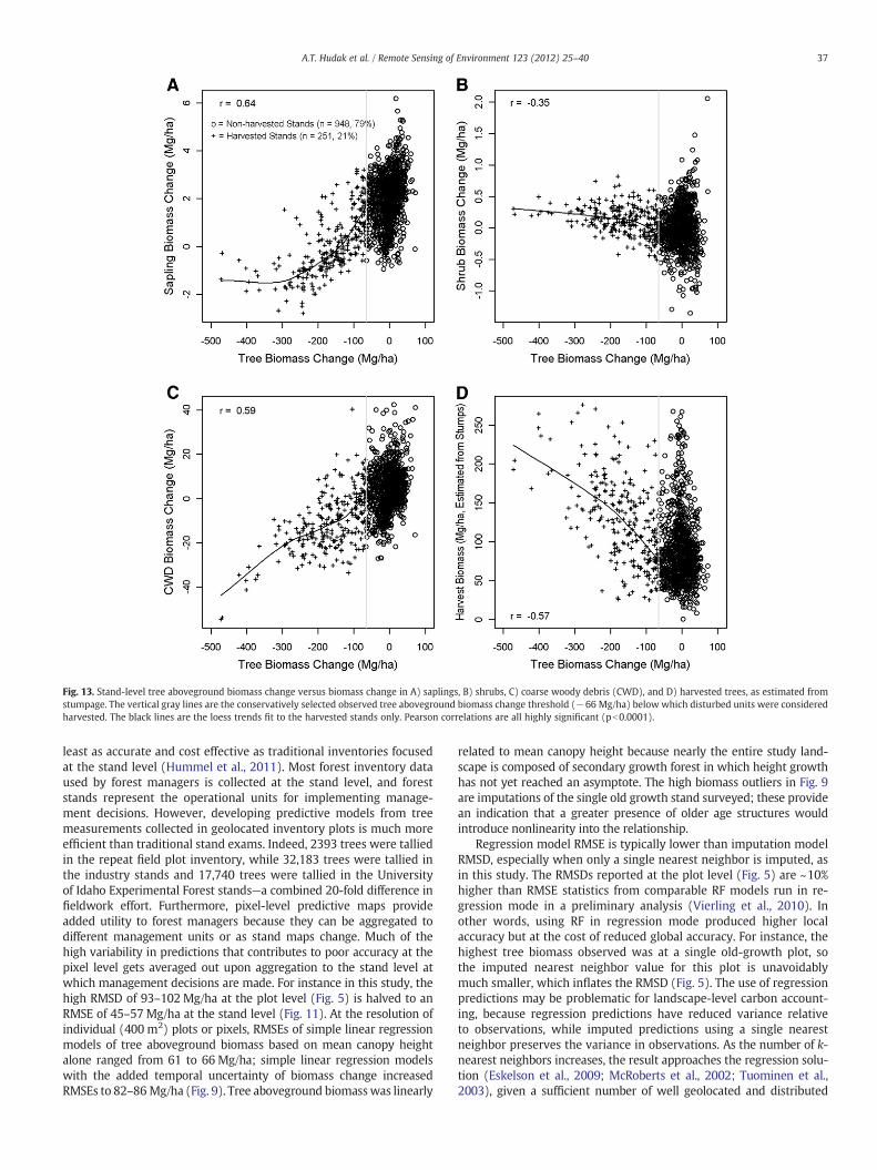
Fig. 13. Stand-level tree aboveground biomass change versus biomass change in A) saplings, B) shrubs, C) coarse woody debris (CWD), and D) harvested trees, as estimated fromstumpage. The vertical gray lines are the conservatively selected observed tree aboveground biomass change threshold (−66 Mg/ha) below which disturbed units were consideredharvested. The black lines are the loess trends fit to the harvested stands only. Pearson correlations are all highly significant (pb0.0001).

37A.T. Hudak et al. / Remote Sensing of Environment 123 (2012) 25–40

least as accurate and cost effective as traditional inventories focusedat the stand level (Hummel et al., 2011). Most forest inventory dataused by forest managers is collected at the stand level, and foreststands represent the operational units for implementing manage-ment decisions. However, developing predictive models from treemeasurements collected in geolocated inventory plots is much moreefficient than traditional stand exams. Indeed, 2393 trees were talliedin the repeat field plot inventory, while 32,183 trees were tallied inthe industry stands and 17,740 trees were tallied in the Universityof Idaho Experimental Forest stands—a combined 20-fold difference infieldwork effort. Furthermore, pixel-level predictive maps provideadded utility to forest managers because they can be aggregated todifferent management units or as stand maps change. Much of thehigh variability in predictions that contributes to poor accuracy at thepixel level gets averaged out upon aggregation to the stand level atwhich management decisions are made. For instance in this study, thehigh RMSD of 93–102 Mg/ha at the plot level (Fig. 5) is halved to anRMSE of 45–57 Mg/ha at the stand level (Fig. 11). At the resolution ofindividual (400 m2) plots or pixels, RMSEs of simple linear regressionmodels of tree aboveground biomass based on mean canopy heightalone ranged from 61 to 66 Mg/ha; simple linear regression modelswith the added temporal uncertainty of biomass change increasedRMSEs to 82–86 Mg/ha (Fig. 9). Tree aboveground biomasswas linearly

related to mean canopy height because nearly the entire study land-scape is composed of secondary growth forest in which height growthhas not yet reached an asymptote. The high biomass outliers in Fig. 9are imputations of the single old growth stand surveyed; these providean indication that a greater presence of older age structures wouldintroduce nonlinearity into the relationship.

Regression model RMSE is typically lower than imputation modelRMSD, especially when only a single nearest neighbor is imputed, asin this study. The RMSDs reported at the plot level (Fig. 5) are ~10%higher than RMSE statistics from comparable RF models run in re-gression mode in a preliminary analysis (Vierling et al., 2010). Inother words, using RF in regression mode produced higher localaccuracy but at the cost of reduced global accuracy. For instance, thehighest tree biomass observed was at a single old-growth plot, sothe imputed nearest neighbor value for this plot is unavoidablymuch smaller, which inflates the RMSD (Fig. 5). The use of regressionpredictions may be problematic for landscape-level carbon account-ing, because regression predictions have reduced variance relativeto observations, while imputed predictions using a single nearestneighbor preserves the variance in observations. As the number of k-nearest neighbors increases, the result approaches the regression solu-tion (Eskelson et al., 2009; McRoberts et al., 2002; Tuominen et al.,2003), given a sufficient number of well geolocated and distributed

38 A.T. Hudak et al. / Remote Sensing of Environment 123 (2012) 25–40

plots (Falkowski et al., 2010; Hudak et al., 2008a,b). Less variance in the2003 and 2009 RF regression model predictions means they wereshifted towards the mean, resulting in an underestimation of biomass/carbon change in both unharvested and harvested forest at the land-scape level (Vierling et al., 2010).

In this paper, equivalence plots of predicted and projectedstand-level biomass in 2003 and 2009 indicated that the meanswere statistically similar but that there was disproportionality thatwas significant in 2003 (Fig. 11). Upon further exploration, wefound that the disproportionate slope term between predicted andprojected stand-level biomass was a function of cruise data inventoryyear. Cruise data more than six years old tended to come from thehigher biomass stands and constituted a higher proportion of the2003 validation (72% from 1997 or earlier) than the 2009 validation(18% from 2003 or earlier). This had the effect of pulling down the lin-ear trendline of best fit in both validations, but especially in 2003(Fig. 11). It may be that the FVS Inland Empire variant predictsgrowth too conservatively compared to the true growth rate on Mos-cow Mountain, because tree aboveground biomass gain due togrowth was projected to be 3.6 Mg/ha/yr versus 4.1 Mg/ha/yr asestimated from LiDAR (Table 3).

Some of the trees within the 75 revisited plots were measured forheight in both field inventories. The mean annual height growth esti-mated from these trees (n=287) was 0.4 m/yr (σ=0.8 m/yr),matching the mean plot-level height growth rate of 0.4 m/yr(σ=0.5 m/yr) reported by Hopkinson et al. (2008) in a mature redpine plantation in southeastern Ontario. Based on maximum LiDARheight measures from four repeat LiDAR surveys spanning five years,Hopkinson et al. (2008) estimated plot-level height growth of 0.38 m/yr(2000–2002), 0.29 m/yr (2002–2004), 0.38 m/yr (2004–2005), and0.34 m/yr overall (2000–2005). This also matches our own estimates ofpixel-level height growth from LiDARmaximum height measures withinthe 146 ha unharvested area where the 2003, 2007, and 2009 LiDARsurveys overlapped: 0.36 m/yr (2003–2007), 0.32 m/yr (2007–2009),and 0.34 m/yr (2003–2009) overall. It is also noteworthy that our studycorroborates awidely reported, slight but consistent LiDAR canopy heightunderestimation bias (Hopkinson et al., 2008; Lim et al., 2003). This likelyexplains why our plot-level tree aboveground biomass predictions wereslightly lower than observations in both 2003 and 2009 (Fig. 7).

4.3. Biomass gains by structural stage and implications for forestmanagement

Assessing biomass accumulation over large areas and extendedtime periods is essential for improving estimates of carbon poolsand fluxes and potential effects on regional- to global-scale carbonbudgets (e.g. DeFries et al., 2002; Houghton et al., 2009; Pan et al.,2011; Strand et al., 2008). For example, forest stand age and rates ofecosystem carbon exchange often exhibit a non-linear relationship,which differs according to species or climate. Law et al. (2003)recorded differences in carbon accumulation rates along a forestchronosequence created by differently aged clearcuts in ponderosapine, and Van Tuyl et al. (2005) extended this work to estimate forestnet primary productivity (NPP) and carbon storage across broaderprecipitation, elevation, disturbance, and species gradients in Oregon.Young regenerating stands exhibited negative NPP values in all casesdue to respiration exceeding photosynthesis, while older standsreached maximum NPP values at different stand ages (i.e., max NPPin moist productive forests occurred in stands b30 years old, whereasmaximum rates in dry forests occurred at a stand age >100 yearsold). Similarly, Schwalm et al. (2007) recorded carbon loss in youngstands (b20 years) followed by an increased ecosystem NPP with in-creased stand age in Douglas-fir in British Columbia. Although struc-tural stages are not necessarily related to stand age, we found thatstructural stages containing mature and old trees stored two to

three times more carbon over the six year time period than did standscomposed of younger trees (Fig. 10).

The majority of the study area is managed for timber productionand harvest has occurred in virtually all stands within the past centu-ry. Therefore, we did not expect to find a decrease in abovegroundbiomass accumulation for any structural stages, even those dominat-ed by large trees (after Law et al., 2003; Fig. 10). This finding has im-plications for forest management, as implementing longer harvestrotations across the study area would likely favor increased carbonuptake at the stand scale, resulting in a landscape-wide increase inaboveground carbon storage through time. As a result, a shift in forestmanagement that would account for the value of standing carbonpools as a function of stand age (e.g. for mitigating atmospheric CO2

emissions), in addition to the value of merchantable timber, maylead to longer harvest rotations in this landscape.

LiDAR is most sensitive to forest attributes related to tree heights(Wulder et al., 2008), yet the imputation modeling approach as wehave demonstrated here allows for simultaneous prediction of otherbiomass/carbon pools besides just the trees (Fig. 7), providing amore comprehensive ecosystem accounting of growth and harvestimpacts (Figs. 12–13). We note that to understand the true tradeoffsin carbon storage with a shift towards a longer harvest managementregime, a life cycle analysis of the forest products created by harvest(e.g., the carbon released and stored via the production, transport,and use of lumber) also should be taken into account (e.g., Pan etal., 2011; Skog & Nicholson, 1998). The carbon accounting tool ofthe Forest Vegetation Simulator is available for this task (Hoover &Rebain, 2008), as is a more recent capability to project growth andcarbon sequestration under alternative climate scenarios (i.e.,Climate-FVS; Crookston et al., 2010). As this study illustrates, treesgrow and sequester carbon slowly compared to how quickly harvestcan deplete carbon stores. Future work with this dataset that involvesstand growth modeling and post-harvest carbon-related life cycleanalyses would likely provide useful predictions for determining op-timal management/harvest cycles for carbon sequestration in thisarea. Further combining these predictions with ground- and LiDAR-based estimates of biodiversity in this area (e.g., Martinuzzi et al.,2009; Vierling et al., 2008; Vogeler et al., in review) would yield amore holistic picture of the ecological implications of changing har-vest regimes.

5. Conclusion

In this study, we demonstrate the utility of using repeat discretereturn airborne LiDAR surveys in concert with field sampling and sta-tistical modeling techniques to quantify spatiotemporal patterns ofaboveground biomass change and carbon flux in a heavily managedconifer forest. We found Moscow Mountain to be a net carbon sourceto the atmosphere during this limited period. Our biomass predic-tions and estimates of biomass change and carbon flux are strictlyempirically derived and are limited to the spatial extent of MoscowMountain and the temporal window of six years. Nevertheless, thisforest is representative of many forests around the globe in that it ismanaged by multiple user groups, including industrial forestry com-panies, private owners, and public land managers. The results of thisstudy indicate that multi-temporal LiDAR may be used to monitorbiomass change and carbon flux across large tracts of actively man-aged forested land.

Forest managers may also want to follow our sampling strategy,because ongoing harvests and other disturbances will alter the popu-lation sampled across the landscape. If the landscape changes due towidespread disturbance, so too would the canopy conditions uponwhich the landscape-level stratification is partially based. While apermanent plot monitoring strategy may be advised for some appli-cations, such as detecting climate change effects, re-stratification ofthe landscape may be the more practical and effective strategy for

39A.T. Hudak et al. / Remote Sensing of Environment 123 (2012) 25–40

repeated biomass inventories of actively managed landscapes such asMoscow Mountain. Projecting future forest carbon sequestration andpotential species shifts under alternative climate and managementscenarios would be a valuable exercise for project planning. AsLiDAR data become continually more available across a range ofbiomes, we expect that the approach outlined in this paper will assistwith quantifying aboveground forest carbon pools and fluxes andtherefore support current and future efforts to mitigate increasinglevels of atmospheric CO2.

Acknowledgements

Primary funding to the University of Idaho for this study was pro-vided by the Department of Energy (DOE) Big Sky C SequestrationPartnership with Montana State and Washington State Universities,with supplemental funding from the U.S. Forest Service RockyMountain Research Station through Joint Venture Agreement 08-JV-11221633-159. Cliff Todd, Sean Taylor, Brendon Newman, and JohnKyle Parker-Mcglynn did the bulk of the 2009 fieldwork. We thankLinda Tedrow and Patrick Adam for LiDAR processing help, andDavid Brown and Steven Mulkey for helpful discussions. We thankHalli Hemingway from Bennett Lumber Products, Inc., Brant Steigersand Rob Taylor from Potlatch Forest Holdings, Inc., and Brian Austinfrom the University of Idaho Experimental Forest, for providingstand exam data used for stand-level validation. Finally, we thankRalph Dubayah and two anonymous reviewers for their helpful sug-gestions on an earlier draft of the manuscript.

References

Asner, G. P., Hughes, R. F., Mascaro, J., Uowolo, A. L., Knapp, D. E., Jacobson, J., et al.(2011). High-resolution carbon mapping on the million-hectare Island of Hawaii.Frontiers in Ecology and the Environment, doi:10.1890/100179 (e-View), 28 pp.

Bater, C. W., Wulder, M. A., Coops, N. C., Nelson, R. F., Hikler, T., & Næsset, E. (2011).Stability of sample-based scanning-LiDAR-derived vegetation metrics for forestmonitoring. IEEE Transactions on Geoscience and Remote Sensing, 49, 2385–2392.

Bones, J. T. (1960). Estimating d.b.h. from stump diameter in the Pacific Northwest. Res.Note. PNW-RN-186. Portland, OR: U.S. Department of Agriculture, Forest Service,Pacific Northwest Forest and Range Experiment Station 2 pp.

Brown, J. K. (1974). Handbook for inventorying downed woody material. Gen. Tech.Rep. INT-16. Odgen, UT: U.S. Department of Agriculture, Forest Service,Intermountain Forest and Range Experiment Station 24 pp.

Brown, J. K. (1981). Bulk densities of nonuniform surface fuels and their application tofire modeling. Forest Science, 27, 677–683.

Brown, J. K., Oberheu, R. D., & Johnston, C. M. (1981). Handbook for inventoryingsurface fuels and biomass in the Interior West. USDA For. Serv. Gen. Tech. Rep.INT-129. Ogden, Utah: Intermt. For. and Range Exp. Stn. 48 pp., 1 84001.

Cooper, S. V., Neiman, K. E., & Roberts, D. W. (1991). Forest habitat types of northernIdaho: A second approximation. Gen. Tech. Rep. INT-236. Ogden, UT: U.S. Depart-ment of Agriculture, Forest Service, Intermountain Research Station 143 pp.

Crookston, N. L., & Finley, A. (2008). yaImpute: An R package for k-NN imputation.Journal of Statistical Software, 23, 1–16 http://www.jstatsoft.org/v23/i10/paper.Package URL: http://cran.r-project.org/web/packages/yaImpute/index.html

Crookston, N. L., Rehfeldt, G. E., Dixon, G. E., & Weiskittel, A. R. (2010). Addressingclimate change in the forest vegetation simulator to assess impacts on landscapeforest dynamics. Forest Ecology and Management, 260, 1198–1211.

DeFries, R. S., Houghton, R. A., Hansen, M. C., Field, C. B., Skole, D., & Townshend, J.(2002). Carbon emissions from tropical deforestation and regrowth based onsatellite observations for the 1980s and 1990s. Proceedings of the NationalAcademy of Sciences of the United States of America, 99, 14256–14261.

Dixon, R. K., Brown, S., Houghton, R. A., Solomon, A. M., Trexler, M. C., & Wisniewski, J.(1994). Carbon pools and flux of global forest ecosystems. Science, 263, 185–190.

Dubayah, R. O., Sheldon, S. L., Clark, D. B., Hofton, M. A., Blair, J. B., Hurtt, G. C., et al.(2010). Estimation of tropical forest height and biomass dynamics using lidarremote sensing at La Selva, Costa Rica. Journal of Geophysical Research,Biogeosciences, 115 17 pp.

Eskelson, B. N. I., Temesgen, H., LeMay, V., Barrett, T. M., Crookston, N. L., & Hudak, A. T.(2009). The roles of nearest neighbor methods in imputing missing data in forestinventory and monitoring databases. Scandinavian Journal of Forest Research, 24,235–246.

Evans, I. S. (1972). General geomorphometry, derivatives of altitude, and descriptivestatistics. In R. J. Chorley (Ed.), Spatial analysis in geomorphology (pp. 17–90).New York: Harper & Row.

Evans, J. S., & Cushman, S. A. (2009). Gradient modeling of conifer species usingRandom Forests. Landscape Ecology, 5, 673–683.

Evans, J. S., & Hudak, A. T. (2007). A multiscale curvature algorithm for classifyingdiscrete return LiDAR in forest environments. IEEE Transactions on Geosciencesand Remote Sensing, 45(4), 1029–1038.

Evans, J. S., Murphy, M. A., Holden, Z. A., & Cushman, S. A. (2010). Modeling speciesdistribution and change using Random Forests. In C. A. Drew, F. Huettmann, & Y.Wiersma (Eds.), Chapter 8 in Predictive modeling in landscape ecology. : Springer.

Falkowski, M. J., Evans, J. S., Martinuzzi, S., Gessler, P. G., & Hudak, A. T. (2009).Characterizing forest succession with lidar data: An evaluation for the inlandnorthwest, USA. Remote Sensing of Environment, 113, 946–956.

Falkowski, M. J., Hudak, A. T., Crookston, N. L., Gessler, P. E., Uebler, E., & Smith, A. M. S.(2010). Landscape-scale parameterization of a tree-level forest growth model: Ak-nearest neighbor imputation approach incorporating LiDAR data. Canadian Jour-nal of Forest Research, 40, 184–199.

Falkowski, M. J., Smith, A. M. S., Gessler, P. E., Hudak, A. T., Vierling, L. A., & Evans, J. S.(2008). The influence of conifer forest canopy cover on the accuracy of twoindividual tree measurement algorithms using LiDAR data. Canadian Journal ofRemote Sensing, 34(S2), S338–S350.

Falkowski, M. J., Smith, A. M. S., Hudak, A. T., Gessler, P. E., Vierling, L. A., & Crookston, N.L. (2006). Automated estimation of individual conifer tree height and crowndiameter via two-dimensional spatial wavelet analysis of lidar data. CanadianJournal of Remote Sensing, 32, 153–161.

FRA (2005). Global Forest Resource Assessment 2005. Progress towards sustainableforest management. Food and Agriculture Organization of the United NationsForestry Paper 147, Viale delle Terme di Caracalla, Rome, Italy Internet access:http://www.fao.org/docrep/008/a0400e/a0400e00.htm

Fu, P., & Rich, P. M. (1999). Design and implementation of the Solar Analyst: AnArcView extension for modeling solar radiation at landscape scales. Proceedingsof the 19th Annual ESRI User Conference, San Diego, USA http://www.fs.fed.us/informs/download.php

Gibbs, H. K., Brown, S., Niles, J. O., & Foley, J. A. (2007). Monitoring and estimatingtropical forest carbon stocks:Making REDD a reality. Environmental Research Letters,2 13 pp.

Goetz, S., & Dubayah, R. (2011). Advances in remote sensing technology andimplications for measuring and monitoring forest carbon stocks and change.Carbon Management, 2(3), 231–244.

Gonzalez, P., Asner, G. P., Battles, J. J., Lefsky, M. A., Waring, K. M., & Palace, M. (2010).Forest carbon densities and uncertainties from LiDAR, QuickBird, and fieldmeasurements in California. Remote Sensing of Environment, 114, 1561–1575.

Harmon, M. E., & Marks, B. (2002). Effects of silvicultural practices on carbon stores inDouglas-fir–western hemlock forests in the Pacific Northwest, U.S.A.: Results froma simulation model. Canadian Journal of Forest Research, 32, 863–877.

Harmon, M. E., & Sexton, J. (1996). Guidelines for measurement of woody detritus inforest ecosystems. Publication No. 20. Seattle, WA: U.S. Long Term EcologicalResearch Network Office, University of Washington, College of Forest Resources73 pp.

Heath, L. S., Smith, J. E., Skog, K. E., Nowak, D. J., & Woodall, C. W. (2010, April/Mayy).Managed forest carbon estimates for the US greenhouse gas inventory,1990–2008. Journal of Forestry, 167–173.

Hines, S. J., Heath, L. S., & Birdsey, R. A. (2010). An annotated bibliography of scientificliterature on managing forests for carbon benefits. Gen. Tech. Rep. NRS-57.Newtown Square, PA: U.S. Department of Agriculture, Forest Service, NorthernResearch Station 49 pp.

Hoover, C., & Rebain, S. (2008). The Kane Experimental Forest carbon inventory: car-bon reporting with FVS. In: Havis, Robert N.; Crookston, Nicholas L., comps. 2008.Third Forest Vegetation Simulator Conference; 2007 February 13–15; Fort Collins,CO. Proceedings RMRS-P-54. Fort Collins, CO: U.S. Department of Agriculture, For-est Service, Rocky Mountain Research Station, pp. 17–22.

Hopkinson, C., Chasmer, L., & Hall, R. J. (2008). The uncertainty in conifer plantationgrowth prediction from multi-temporal lidar datasets. Remote Sensing ofEnvironment, 112, 1168–1180.

Houghton, R. A., Hall, F., & Goetz, S. J. (2009). Importance of biomass in the globalcarbon cycle. Journal of Geophysical Research, Biogeosciences, 114 13 pp.

Hudak, A. T., Crookston, N. L., Evans, J. S., Falkowski, M. J., Smith, A. M. S., Gessler, P. E.,et al. (2006). Regression modeling and mapping of coniferous forest basal area andtree density from discrete-return lidar and multispectral satellite data. CanadianJournal of Remote Sensing, 32, 126–138.

Hudak, A. T., Crookston, N. L., Evans, J. S., Hall, D. E., & Falkowski, M. J. (2008a). Nearestneighbor imputation of species-level, plot-scale forest structure attributes fromLiDAR data. Remote Sensing of Environment, 112, 2232–2245.

Hudak, A. T., Evans, J. S., Crookston, N. L., Falkowski, M. J., Steigers, B., Taylor, R., &Hemingway, H. (2008b). Aggregating pixel-level basal area predictions derived fromLiDAR data to industrial forest stands in Idaho. In: Havis, Robert N.; Crookston,Nicholas L., comps. Third Forest Vegetation Simulator Conference; 2007 February13–15; Fort Collins, CO. Proceedings RMRS-P-54. Fort Collins, CO: U.S. Department ofAgriculture, Forest Service, Rocky Mountain Research Station. pp. 133–146.

Hudak, A. T., Evans, J. S., & Smith, A. M. S. (2009). Review: LiDAR utility for naturalresource managers. Remote Sensing, 1, 934–951, doi:10.3390/rs1040934.

Hudak, A. T., Lefsky, M. A., Cohen, W. B., & Berterretche, M. (2002). Integration of LiDARand Landsat ETM+ data for estimating and mapping forest canopy height. RemoteSensing of Environment, 82, 397–416.

Hummel, S., Hudak, A. T., Uebler, E. H., Falkowski, M. J., & Megown, K. A. (2011,July/August). A comparison of accuracy and cost of LiDAR versus stand examdata for landscape management on the Malheur National Forest. Journal ofForestry, 267–273.

Jain, T.B., Graham, R.T., & Adams, D. (2010). Carbon concentrations and carbon pool dis-tributions in dry, moist, and cold mid-aged forests of the Rocky Mountains. In: Jain,

40 A.T. Hudak et al. / Remote Sensing of Environment 123 (2012) 25–40

T.B., Graham, R.T., and Sandquist, J. tech eds. Integrated management of carbon se-questration and biomass utilization opportunities in a changing climate. Proceed-ings of the 2009 National Silvicultural Workshop, 2009 June 15–18, Boise, ID.Proceedings RMRS-P-61. Fort Collins, CO: U.S. Department of Agriculture, ForestService, Rocky Mountain Research Station. 351 p.

Jenkins, J. C., Chojnacky, D. C., Heath, L. S., & Birdsey, R. A. (2003). National-scalebiomass estimators for United States tree species. Forest Science, 49, 12–35.

Kimsey, M. J., Jr., Garrison-Johnston, M. T., & Johnson, L. (2011). Characterization ofvolcanic ash-influenced forest soils across a geoclimatic sequence. Soil ScienceSociety of America Journal, 75, 267–279.

Law, B. E., Sun, O. J., Campbell, J., Van Tuyl, S., & Thornton, P. E. (2003). Changes incarbon storage and fluxes in a chronosequence of ponderosa pine. Global ChangeBiology, 9, 510–524.

Lefsky, M. A., Cohen, W. B., Harding, D. J., Parker, G. G., Acker, S. A., & Gower, S. T.(2002). LiDAR remote sensing of aboveground biomass in three biomes. GlobalEcology and Biogeography, 11, 393–399.

Lim, K., Treitz, P., Wulder, M., St-Onge, B., & Flood, M. (2003). Lidar remote sensing offorest structure. Progress in Physical Geography, 27, 88–106.

Martinuzzi, S., Vierling, L. A., Gould, W. A., Falkowski, M. J., Evans, J. S., Hudak, A. T., et al.(2009). Mapping snags and understory shrubs for a LiDAR-based assessment ofwildlife habitat suitability. Remote Sensing of Environment, 113, 2533–2546.

McCune, B., & Keon, D. (2002). Equations for potential annual direct incident radiationand heat load index. Journal of Vegetation Science, 13, 603–606.

McKinley, D. C., Ryan, M. G., Birdsey, R. A., Giardina, C. P., Harmon, M. E., Heath, L. S.,et al. (2011). A synthesis of current knowledge on forests and carbon storage inthe United States. Ecological Applications, 21, 1902–1924.

McNab, H. W. (1989). Terrain shape index: Quantifying effect of minor landforms ontree height. Forest Science, 35(1), 91–104.

McRoberts, R. E., Nelson, M. D., & Wendt, D. G. (2002). Stratified estimation of forestarea using satellite imagery, inventory data, and the k-nearest neighbors tech-nique. Remote Sensing of Environment, 82, 457–468.

Moore, I. D., Gessler, P. E., Nielsen, G. A., & Petersen, G. A. (1993). Terrain attributes:Estimation methods and scale effects. In A. J. Jakeman, M. B. Beck, & M. McAleer(Eds.), Modeling change in environmental systems (pp. 189–214). London: Wiley.

Murphy, M. A., Evans, J. S., & Storfer, A. S. (2010). Quantify Bufo boreas connectivity inYellowstone National Park with landscape genetics. Ecology, 91, 252–261.

Nemani, R., Pierce, L., Running, S., & Band, L. (1993). Forest ecosystem processes at thewatershed scale: Sensitivity to remotely-sensed Leaf Area Index estimates. Interna-tional Journal of Remote Sensing, 14, 2519–2534.

Nilsson, M. (1996). Estimation of tree heights and stand volume using an airborneLiDAR system. Remote Sensing of Environment, 56, 1–7.

O'Hara, L. O., Latham, P. A., Hessburg, P., & Smith, B. G. (1996). A structural classificationfor inland Northwest forest vegetation. Western Journal of Applied Forestry, 11,97–102.

Pan, Y. D., Birdsey, R. A., Fang, J. Y., Houghton, R., Kauppi, P. E., Kurz, W. A., et al. (2011).A large and persistent carbon sink in the world's forests. Science, 333, 988–993.

Parker, A. J. (1982). The topographic relative moisture index: An approach tosoil-moisture assessment in mountain terrain. Physical Geography, 3, 160–168.

Pike, R. J., & Wilson, S. E. (1971). Elevation relief ratio, hypsometric integral, andgeomorphic area altitude analysis. Bulletin of the Geological Society of America, 82,1079–1084.

R Development Core Team (2007). R: A language and environment for statistical comput-ing. Vienna, Austria: R Foundation for Statistical Computing Access: http://www.R-project.org

Riley, S. J., DeGloria, S. D., & Elliot, R. (1999). A terrain ruggedness index that quantifiestopographic heterogeneity. Intermountain Journal of Sciences, 5(1–4), 1999.

Roberts, D. W., & Cooper, S. V. (1989). Concepts and techniques of vegetation mapping.Land classifications based on vegetation: Applications for resource management.GTR-INT-257 (pp. 90–96). Ogden, UT: USDA Forest Service IntermountainResearch Station.

Robinson, A. P., Duursma, R. A., & Marshall, J. D. (2005). A regression-based equivalencetest for model validation: Shifting the burden of proof. Tree Physiology, 25,903–913.

Saatchi, S. S., Harris, N. L., Brown, S., Lefsky, M., Mitchard, E. T. A., Salas, W., et al. (2011).Benchmark map of forest carbon stocks in tropical regions across three continents.Proceedings of the National Academy of Sciences, 108, 9899–9904, www.pnas.org/cgi/doi/10.1073/pnas.1019576108

Schwalm, C. R., Black, T. A., Morgenstern, K., & Humphreys, E. R. (2007). A method forderiving net primary productivity and component respiratory fluxes fromtower-based eddy covariance data: A case study using a 17-year data recordfrom a Douglas-fir chronosequence. Global Change Biology, 13, 370–385.

Skog, K. E., & Nicholson, G. A. (1998). Carbon cycling through wood products: The roleof wood and paper products in carbon sequestration. Forest Products Journal, 48,75–83.

Smith, W. B., & Brand, G. J. (1983). Allometric Biomass Equations for 98 species ofherbs, shrubs, and small trees. North Central Forest Experiment Station, ResearchNote NC-299 8 pp.

Stage, A. R. (1976). An expression of the effects of aspect, slope, and habitat type ontree growth. Forest Science, 22(3), 457–460.

Stage, A. R., & Crookston, N. L. (2007). Partitioning error components foraccuracy-assessment of near-neighbor methods of imputation. Forest Science, 53,62–72.

Stoker, J., Harding, D., & Parrish, J. (2008). The need for a National Lidar Dataset.Photogrammetric Engineering and Remote Sensing, 74, 1066–1068.

Strand, E. K., Vierling, L. A., Smith, A. M. S., & Bunting, S. C. (2008). Net changes inaboveground woody carbon stock in western juniper woodlands, 1946–1998.Journal of Geophysical Research, 113, G01013, doi:10.1029/2007JG000544.

Tuominen, S., Fish, S., & Poso, S. (2003). Combining remote sensing, data from earlierinventories, and geostatistical interpolation in multisource forest inventory.Canadian Journal of Forest Research, 33, 624–634.

Van Tuyl, S., Law, B. E., Turner, D. P., & Gitelman, A. I. (2005). Variability in net primaryproduction and carbon storage in biomass across Oregon forests — An assessmentintegrating data from forest inventories, intensive sites, and remote sensing. ForestEcology and Management, 209, 273–291.

Vierling, L. A., Hudak, A. T., Strand, E. K., Eitel, J. U. H., & Martinuzzi, S. (2010). Quanti-fying forest aboveground carbon pools and fluxes using multi-temporal LiDAR.Unpublished report, Big Sky Carbon Sequestration Partnership Forestry Team, 33pp.

Vierling, L. A., Martinuzzi, S., Asner, G. P., Stoker, J., & Johnson, B. R. (2011). Lidar:providing structure. Frontiers in Ecology and the Environment, 9, 261–262, doi:10.1890/11.WB.009.

Vierling, K. T., Vierling, L. A., Gould, W. A., Martinuzzi, S., & Clawges, R. M. (2008). Lidar:shedding new light on habitat characterization and modeling. Frontiers in Ecologyand the Environment, 6, 90–98.

Vine, E., & Sathaye, J. (1997). The monitoring, evaluation, reporting, and verification ofclimate change mitigation projects: Discussion of issues and methodologies andreview of existing protocols and guidelines. EPA Report LBNL-40316.

Vogeler, J. C., Vierling, K. T., Hudak, A. T., & Vierling, L. A. (in review). LiDAR-derivedcanopy architecture allows occupancy prediction of Brown Creepers in two west-ern coniferous forests. The Condor.

Woodall, C. W., & Monleon, V. J. (2006). Estimating the quadratic mean diameter of finewoody debris for forest type groups of the United States. Proceedings of the EighthAnnual Forest Inventory and Analysis Symposium (pp. 185–190).

Wooldridge, D. D. (1968). Chemical and physical properties of forest litter layers incentral Washington. Tree Growth and Forest Soils, Proc. Third North Am. For. SoilsConf. [N.C. State Univ., Aug. 1968] (pp. 327–337).

Wulder, M. A., Bater, C. W., Coops, N. C., Hilker, T., & White, J. C. (2008). The role ofLiDAR in sustainable forest management. The Forestry Chronicle, 84, 807–826.

Yu, X., Hyyppä, J., Kaartinen, H., & Maltamo, M. (2004). Automatic detection ofharvested trees and determination of Forest growth using airborne laserscanning. Remote Sensing of Environment, 90, 451–462.

Yu, X., Hyyppä, J., Kaartinen, H., Maltamo, M., & Hyyppä, H. (2008). Obtaining plotwisemean height and volume growth in boreal forests using multi-temporal laser sur-veys and various change detection techniques. International Journal of RemoteSensing, 29, 1367–1386.