ISSN 0956-8549-610

Can Rare Events Explain the Equity Premium Puzzle?

Christian Julliard

Anisha Ghosh

DISCUSSION PAPER NO 610

DISCUSSION PAPER SERIES

March 2008 Christian Julliard is a Lecturer in the Department of Economics and senior research associate of the Financial Market Group at the London School of Economics and Political Science. He is also a research affiliate of the Centre for Economic Policy Research (CEPR) and editorial board member of the Review of Economic Studies. He was awarded a Ph.D. by the Department of Economics at Princeton University where he was also affiliated with the Bendheim Center for Finance and the Woodrow Wilson School of Public and International Affairs. Anisha Ghosh is a PhD student in the Department of Economics at London School of Economics and Political Science. She completed her BSc in Economics from Presidency College, Calcutta in 2003 and then the MRes in Economics at London School of Economics and Political Science in 2005. Any opinions expressed here are those of the authors and not necessarily those of the FMG. The research findings reported in this paper are the result of the independent research of the authors and do not necessarily reflect the views of the LSE.

Can Rare Events Explain the Equity PremiumPuzzle?�

Christian Julliardy

Department of EconomicsLondon School of Economics

Anisha Ghoshz

Department of EconomicsLondon School of Economics

First version: October 2007. This version: March 7, 2008.

AbstractProbably not. First, allowing the probabilities attached to the states of the

economy to di¤er from their sample frequencies, the Consumption-CAPM is stillrejected by the data and requires a very high level of Relative Risk Aversion(RRA) in order to rationalize the stock market risk premium. This result holdsfor a variety of data sources and samples � including ones starting as far backas 1890. Second, we elicit the likelihood of observing an Equity Premium Puz-zle (EPP) if the data were generated by the rare events probability distributionneeded to rationalize the puzzle with a low level of RRA. We �nd that the his-torically observed EPP would be very unlikely to arise. Third, we �nd thatthe rare events explanation of the EPP signi�cantly worsens the ability of theConsumption-CAPM to explain the cross-section of asset returns. This is due tothe fact that, by assigning higher probabilities to bad �economy wide �statesin which consumption growth is low and all the assets in the cross-section tendto yield low returns, the rare events hypothesis reduces the cross-sectional dis-persion of consumption risk relative to the cross-sectional variation of averagereturns.Keywords: Rare Events, Rare Disasters, Equity Premium Puzzle, Generalized Empiri-cal Likelihood, Semi-parametric Bayesian Inference, Calibration, Cross-Section of AssetReturns, Peso Phenomenon. JEL classi�cation: C11, C14, E17, G12.

�We bene�ted from helpful comments from Markus Brunnermeier, Francesco Caselli, George Con-stantinides, Jean-Pierre Danthine, Bernard Dumas, Xavier Gabaix, Oliver Linton, Sydney Ludvigson,Alex Michaelides, Jonathan Parker, Lubos Pastor, Dimitri Vayanos, Pietro Veronesi, Amir Yaron andseminar participants at the CEP/LSE Money-Macro workshop, Ente Einaudi, FMG/LSE workshop,HEC Paris, New York Fed, Paris School of Economics, Royal Holloway, Sorbonne University, UCIrvine.

yDepartment of Economics and FMG, London School of Economics, Houghton Street, LondonWC2A 2AE, U.K., and CEPR, C.Julliard@lse.ac.uk, http://personal.lse.ac.uk/julliard/.

zDepartment of Economics, London School of Economics, Houghton Street, London WC2A 2AE,U.K., a.ghosh@lse.ac.uk, http://personal.lse.ac.uk/ghosh/.

1 Introduction

The average excess return on the U.S. stock market relative to the one-month Trea-sury Bill �the so called equity risk premium �has been about 7% per year over thelast century. Nevertheless, the representative agent model with time separable CRRAutility, calibrated to match micro evidence on households�attitude toward risk andthe time series properties of consumption and asset returns, generates a risk premiumof less than 1%. This quantitative discrepancy was originally dubbed by Mehra andPrescott (1985) as the Equity Premium Puzzle (EPP). Given the dramatic long-terminvestment implications of this di¤erential rate of return, over the last two decades theequity premium puzzle has been the focus of a substantial research e¤ort in Economicsand Finance.1

In this paper we study the ability of the rare events hypothesis, pioneered by Rietz(1988) and recently revived by a growing literature (e.g. Veronesi (2004), Barro (2006),Gabaix (2007a)), to rationalize the equity premium puzzle. This hypothesis is concep-tually simple. Suppose that in every period there is an ex ante small probability of anextreme stock market crash and economic downturn (that is, a Great Depression-likestate of the economy). Risk averse equity owners will demand a high equity premiumto compensate for the extreme losses they may incur during these unlikely �but ex-ceptionally harmful �states of the world. In a �nite sample, if such states happen tooccur with a frequency lower than their true probability, ex post realized risk premiawill be high even though ex ante expected returns are low �that is, in such a scenarioequity owners are compensated for crashes and economic contractions that happen notto occur. Moreover, to an outside observer investors will appear irrational in the sam-ple, and economists will tend to overestimate their risk aversion and underestimate theconsumption risk of the stock market.Our contribution to the analysis of the rare events hypothesis is three-fold. First,

adopting an information-theoretic alternative to the Generalized Method of Moments2

(see Owen (1991, 2001), Kitamura and Stutzer (1997), Kitamura (2006)), we estimatethe consumption Euler equation for the equity risk premium allowing explicitly theprobabilities attached to di¤erent states of the economy to di¤er from their samplefrequencies. We �nd that the Consumption Capital Asset Pricing Model (C-CAPM)is still rejected by the data, and requires a very high level of relative risk aversion inorder to rationalize the stock market risk premium. Moreover, this result holds for avariety of data sources and samples, including ones that start as far back as 1890 andthat cover extreme historical events such as the Great Depression and the World Wars.The econometric methodologies we use belong to the Generalized Empirical Like-

lihood family, and i) are by construction more robust to a rare events problem in the

1However, according to Mehra and Prescott (2003), none of the proposed explanations has beenso far fully satisfactory (see also Campbell (1999, 2003)).

2Hansen (1982) and Hansen and Singleton (1982).

1

data,3 ii) tend to have better small sample and asymptotic properties than the stan-dard GMM approach (see e.g. Kunitomo and Matsushita (2003), Newey and Smith(2004) and Kitamura (2006)), iii) allow us to perform Bayesian posterior inference(Lazar (2003), Schennach (2005)) that does not rely on asymptotic properties that areless likely to be met, in �nite sample, in the presence of rare events.Moreover, we show that our information-theoretic estimation approaches can also

be used to identify, nonparametrically, the rare events distribution needed to rationalizethe equity premium puzzle with a low level of risk aversion. In contrast with the ad hocdistributional assumptions and calibrations used in the previous literature on the rareevents hypothesis, our methodology identi�es the closest distribution, in the Kullback-Leibler Information sense, to the true unknown distribution of the data. That is, itprovides the most likely rare events explanation of the equity premium puzzle. Weshow that our identi�ed rare events distributions are in line with the ones advocatedby Rietz (1988) and Barro (2006) �that is, our data-driven procedure �nds that onlymodest increases in the likelihood of observing extremely bad states such as the GreatDepression are needed to rationalize the equity premium puzzle.Second, with these estimated rare events distributions at hand, we generate coun-

terfactual histories of data of the same length as the historical time series. This allowsus to elicit the probability of observing an equity premium puzzle in samples of thesame size as the historical ones. We �nd that if the data were generated by the rareevents distribution needed to rationalize the equity premium puzzle with a low levelof risk aversion, the puzzle itself would be very unlikely to arise. We interpret this�nding as suggesting that, if one is willing to believe that the rare events hypothesis isthe explanation of the equity premium puzzle, one should also believe that the puzzleitself is a rare event.Third, we study whether rare events can rationalize the poor performance of the

Consumption-CAPM in pricing the cross-section of asset returns. We �nd that impos-ing on the data the rare events explanation of the equity premium puzzle worsens theability of the Consumption-CAPM to explain the cross-section of asset returns. This isdue to the fact that, in order to rationalize the equity premium puzzle with a low levelof risk aversion, we need to assign higher probabilities to bad �economy wide �statessuch as deep recessions and market crashes. Since during market crashes and deeprecessions consumption growth tends to be low and all the assets in the cross-sectiontend to yield low returns, this reduces the cross-sectional dispersion of consumptionrisk across assets, making it harder for the model to explain the cross-section of riskpremia. This �nding also suggests that explanations of the equity premium puzzlebased on agents�expectations of an economy wide disaster (e.g. a �nancial marketmeltdown) that has not materialized in the sample �a so called peso phenomenon �

3This is due both to the Large Deviations properties of our estimation and testing approaches (seee.g. Kitamura (2006)), and to the �weak law of large numbers for rare events�rationale for estimatorsbased on relative entropy minimization (Brown and Smith (1990)).

2

would also reduce the ability of the Consumption-CAPM to price the cross-section ofasset returns, since such an expectation would reduce the cross-sectional dispersion ofconsumption risk across assets.We interpret the above set of results as suggesting that the rare events hypothesis

is an unlikely explanation of the equity premium puzzle. This conclusion is partiallyin contrast with the calibration evidence in Barro (2006). We analyze this discrepancyformally, and show that it can be explained by the fact that Barro�s calibration is likelyto overstate the consumption risk due to rare economic disasters since i) he calibrates ayearly model using the cumulated multi-year contraction observed during disasters, andii) he assumes that the consumption drop during disasters is equal to the contractionin GDP.The paper also provides an important methodological contribution, since the (non

parametric) information theoretic approach to calibration we propose can be appliedto any economic model that delivers well de�ned moment conditions. This approachhas the appealing feature of making the calibrated model as close as possible �in theinformation sense �to the true unknown one, and enables model evaluation that is freefrom ancillary distributional assumptions.The remainder of the paper is organized as follows. Section 2 reviews the related lit-

erature on the rare events hypothesis. Section 3 presents the theoretical underpinningsof the estimation and testing approaches considered. A data description is providedin Section 4. Estimation and testing results are presented in Sections 5. Section 6.1presents the rare events distribution of the data needed to rationalize the equity pre-mium puzzle with a low level of risk aversion. In Section 6.2, we ask what would be thelikelihood of observing an equity premium puzzle, in samples of the same size as thehistorical ones, if the rare events hypothesis were the true explanation of the puzzle. InSection 6.3, we analyze the implications of the rare events hypothesis for the ability ofthe C-CAPM to price the cross-section of asset returns. Section 7 analyzes the discrep-ancy between our results and those in Barro (2006). Section 8 concludes. Additionalrobustness checks, and methodological details, are provided in the Appendix.

2 Rare Events �Related Literature

�Un coup de dés jamais n�abolira le hasard.�4 Mallarmé (1897).

In this section we sketch the links to the existing literature on the rare events hypoth-esis.Already in the sixties Mandelbrot (1963, 1967) pointed out that extreme �nancial

asset price swings are more likely than what is often assumed in our models, and thatreturns on risky assets tend to have much thicker tails than a Gaussian distribution.

4�A throw of dice will never abolish chance.�

3

The need of dealing with these empirical regularities is at the origin of: the attempts toapply extreme value theory (a branch of statistics that focuses on extreme deviationsfrom the median) to quantitative �nancial analysis (see e.g. Beirlant, Schoutens, andSegers (2004)); the popularity, within the risk management industry, of the value-at-risk approach for assets valuation (the VaR measures the worst anticipated loss over aperiod); the inclusion of jump and Lévy processes into derivatives pricing models, andthe development of tail-related �nancial risk measures.The �rst to suggest that tail events in the distribution of asset returns and con-

sumption might be the reason behind the equity premium puzzle originally documentedby Mehra and Prescott (1985), is Rietz (1988). As Mehra and Prescott, Rietz consid-ers a (Markovian) �nite-state version of the Lucas (1978) exchange economy. In thissetting (as in the Consumption-CAPM of Rubinstein (1976) and Breeden (1979)), theoptimizing behavior of the agent leads to the consumption Euler equation

E

"�CtCt�1

�� Ret

#= 0; (1)

where E is the unconditional expectation operator, Ct denotes the time t consumption�ow, is the relative risk aversion coe¢ cient, and Ret is the return on the stock marketin excess of the risk free rate.The only di¤erence between the Mehra-Prescott and the Reitz frameworks is that

in the former the state of the economy is good or bad with equal probabilities, whilethe latter adds a low probability depression-like state to capture rare, but severe,economic downturns and market crashes. Calibrating the depression state to matchthe economic contraction registered during the Great Depression, Rietz �nds that a lessthan 2% probability for such a state is enough to make the model match the historicallyobserved equity premium. Moreover, Danthine and Donaldson (1999) show that sucha result also holds in a production economy setting.More recently, Barro (2006) constructs a model of the equity-premium that ex-

tends Rietz (1988), and calibrates disaster probabilities from the twentieth centuryglobal history �especially the sharp contractions associated with the Great Depressionand the World Wars. He argues that the potential for rare economic disasters explainsa lot of asset pricing puzzles including the high equity premium, the low risk-free rate,and volatile stock returns. Gabaix (2007a), combining the Reitz�s hypothesis with ananalytically tractable assumption about the data generating processes (the �linearity-generating processes�of Gabaix (2007b)), argues that rare events can potentially ra-tionalize not only the equity premium, but also nine more puzzles in macro-�nance.Similarly, but adding agents�learning to the framework, Veronesi (2004) concludes thatthe peso problem hypothesis implies most of the stylized facts about stock returns, in-cluding time-varying volatility, asymmetric volatility reaction to good and bad news,

4

and excess sensitivity of price reaction to dividend changes.5 On the contrary, Gourio(2008a, 2008b) �nds that the rare events model has counterfactual implications for thepredictability of asset returns.Beside the equity premium, the concept of rare events has also been applied to

the study of a wide array of subjects such as: the term structure of interest rates,6

exchange rates �uctuations and the forward-premium puzzle,7 households�investmentin annuities8 and saving decisions,9 the �smirk� patterns documented in the indexoptions market.10

The common characteristic of all the studies that have focused on the rare eventshypothesis and the equity premium puzzle, is the use of a calibration approach.11 Sincethe equity premium is a �rst moment, and �rst moments are extremely sensitive tooutliers, results in the rare events setting tend to be very sensitive to the calibrationchoice. For example, Copeland and Zhu (2006) extend the Barro (2006) closed-economymodel to a two country setting, and they show that �using Barro�s own calibration �themodel implies levels of the equity risk premium far lower than those typically observedin the data e.g. they reverse Barro�s original �nding by allowing for internationaldiversi�cation.An obvious alternative to calibration is to estimate directly the consumption Euler

equation (1), and this has been done extensively in the literature. The standard ap-proach is to use consumption and stock market data to estimate the relative riskaversion parameter, , in equation (1) as

:= argmin g

ET

"�CtCt�1

�� Ret

#; ET [Ret ] ; E

T

"�CtCt�1

�� #!(2)

for some function g (:), where ET [xt] = 1T

PTt=1 xt i.e. the distributions of the pricing

kernel and returns is proxied with an empirical distribution that assigns probability1=T to each realized state (observation) in the sample, and then judge whether (orsome function of , like the implied expected returns or a test statistic) is �reasonable.�The GMM inference, for example, belongs to this class (see Hansen (1982), Hansen and

5See also Sandroni (1998) on the interaction between learning and rare events.6See e.g. Lewis (1990) and Bekaert, Hodrick, and Marshall (2001).7Gourinchas and Tornell (2004) and Farhi and Gabaix (2007).8Lopes and Michaelides (2007).9Carroll (1997).10Liu, Pan, and Wang (2005).11Some indirect empirical evidence supporting the rare events hypothesis can be found in Brown,

Goetzmann, and Ross (1995) and Goetzmann and Jorion (1999a) (see also Goetzmann and Jorion(1999b)). The �rst of these papers shows that the time series of equity returns on the U.S. stockmarket might be a¤ected by survival bias. The second considers a large international cross-section ofmarket returns, and �nds that the average high return on the U.S. stock market belongs to the righttail of the cross-sectional distribution.

5

Singleton (1982)). In some cases, distributional assumptions are directly made, and theinference is conditional on this (e.g log-normal returns and consumption growth). Thereplacement of the unconditional moments with sample moments is justi�ed by weaklaw of large numbers and central limit arguments. Nevertheless, in a �nite sample,the presence of extreme rare events, that happen to occur with a lower (or higher)frequency than their true probability, can have dramatic e¤ects on the sample �rstmoments. Therefore, inference based on equation (2) might be unreliable. Saikkonnenand Ripatti (2000) illustrate this point with a Monte Carlo exercise, and they documentan extremely poor performance of the GMM estimator of the Euler equation in thepresence of rare events �even in relatively large samples.Two conclusions can be drawn from the above review of the literature. First,

in calibrating a rare events model, we would ideally remove any degree of freedomregarding the modeling of the underlying true distribution of the data. That is, itwould be desirable to a) avoid parametric assumptions about the distribution of thedata, and b) use an approach that makes the calibrated distribution as close as possibleto the true, unknown, distribution of the data.Second, in estimating and testing the consumption Euler equation in the presence

of a potential rare events phenomenon, it would be desirable to use an approach thatallows the probabilities attached to di¤erent states of the economy to di¤er from theirsample frequencies �that is, an approach that explicitly allows to take rare events intoaccount.Our paper does both of these things, and additionally derives the implications of

imposing the rare events explanation of the equity premium puzzle on the cross-sectionof asset returns �a feature that, to the best of our knowledge, we are the �rst to analyze.

3 Econometric Methodology

The econometric methodology we employ belongs to the Generalized Empirical Likeli-hood family. In particular, we use four estimation and testing approaches: the Empir-ical Likelihood (EL) of Owen (1988, 1990, 1991), the Exponential Tilting (ET) of Ki-tamura and Stutzer (1997), the Bayesian Empirical Likelihood (BEL) of Lazar (2003),and the Bayesian Exponentially Tilted Empirical Likelihood (BETEL) of Schennach(2005). These approaches are chosen for their suitability to analyze data that might bea¤ected by a rare events phenomenon. In what follows we present these econometricmethodologies and discuss their advantages in the presence of a rare events problemin the data. Readers familiar with this econometric literature can skip this sectionwithout loss of continuity.Consider a model characterized by the following moment condition

E� [f(zt; �0)] �Zf(zt; �0)d� = 0, � 2 � � Rs, (3)

6

where f is a known Rq-valued function, q > s, and 0 denotes a vector of zeros ofsize q. The econometrician observes draws of an Rk-valued random variable, fztgTt=1,where each zt is distributed according to an unknown probability measure �, and �0denotes the true �unknown �value of �. The approaches used in this paper can beapplied to both i:i:d: or (weakly) dependent data.12 In the case of i:i:d. observationsthe nonparametric log likelihood at (p1; p2; :::; pT ) is

`NP (p1; p2; :::; pT ) =

TXt=1

log(pt); (p1; :::; pT ) 2 � (4)

where � denotes the simplexn(p1; :::; pT ) :

PTt=1 pt = 1, pt � 0, t = 1; :::; T

o: This

last expression can be interpreted as the log likelihood for a multinomial model, wherethe support of the multinomial distribution is given by the empirical observations,fztgTt=1, even though the distribution � of zt is not assumed to be multinomial �it isindeed left unspeci�ed. The Empirical Likelihood (EL) estimator of Owen (1988, 1990,1991) parametrizes the moment condition (3) with (�; p1; p2; :::; pT ) 2 � � �, and isgiven by

�b�EL; bpEL1 ; :::; bpELT � = argmaxf�;p1;:::;pT g2���

`NP =TXt=1

log(pt) subject toTXt=1

f(zt; �)pt = 0:

(5)

subject toTXt=1

f(zt; �)pt = 0:

Thus, the EL estimation de�nes a function that appears analogous to a parametriclikelihood function and yet enables inference that does not require distributional as-sumptions. Moreover, the nonparametric maximum likelihood estimator (NPMLE) ofthe unknown probability measure � is given by �EL =

PTt=1 bpELt �zt, where �z denotes

a unit mass at z. This is an e¢ cient estimator for �, i.e. for a function a(z; �0) ofz,PT

t=1 a(zt;b�EL)bpELt is a more e¢ cient estimator of E [a(z; �0)] than the naive sam-

ple mean 1T

PTt=1 a(zt;

b�EL), and can be shown to be semiparametrically e¢ cient (seeKitamura (2006) and Brown and Newey (1998)).The EL estimator, for both i:i:d: and weakly dependent data, also has an important

information-theoretic interpretation (see e.g. Kitamura and Stutzer (1997)). To seethis let M be the set of all probability measures on Rk, and for each parameter vector� 2 �, de�ne the following set of probability measures

P (�) � fp 2M : Ep [f(zt; �)] = 0g (6)

12See e.g. Kitamura (1997) for a de�nition of weak dependence.

7

which are also absolutely continuous with respect to the measure � in equation (3).Therefore, P � [�2�P (�) is the set of all the probability measures that are consis-tent with the model characterized by the moment condition in equation (3). The ELestimator can be shown to solve the following optimization problem

inf�2�

infp2P (�)

K(�; p) = inf�2�

infp2P (�)

Zlog (d�=dp) d�, (7)

subject to Ep [f(zt; �)] = 0;

where K(�; p) is the Kullback-Leibler Information Criterion (KLIC) divergence from �to p (White (1982)). Therefore K(�; p) > 0, and it will hold with equality if and onlyif � = p. If the model is correctly speci�ed, i.e. if there exists a �0 satisfying (3), wehave that � 2 P (�0), and � solves (7) delivering a KLIC value of 0. On the other hand,if the model is misspeci�ed, � is not an element of P and for each � there is a positiveKLIC distance K(�; p) > 0 attained by the solution p(�). Thus, the EL approachsearches for a �EL (�) that makes the estimated distribution as close as possible �inthe information sense �to the true unknown one.Since the KLIC is not symmetric, the closely related Exponential Tilting (ET)

estimator of Kitamura and Stutzer (1997) can be obtained by inverting the roles of �and p in (7). That is, the ET estimator solves

b�ET = inf�2�

infp2P (�)

K(p; �) = inf�2�

infp2P (�)

Zlog (dp=d�) dp; (8)

subject to Ep [f(zt; �)] = 0:

To �rst order, the ET and EL estimators are asymptotically equivalent to theoptimal GMM estimator (Kitamura and Stutzer (1997), Qin and Lawless (1994)), i.e.have an asymptotic normal distribution given by

pT�b�j � �0� d! N(0; V ), j 2 fEL;ETg (9)

V = (D0S�1D)�1, D = E� [@f(z;�0)=@�0] , S = E� [f(z;�0)f(z;�0)

0]

However, Newey and Smith (2004) show that these estimators have smaller second-order bias than the GMM estimator. They also show that the bias-corrected EL es-timator is third-order e¢ cient. Moreover, Kunitomo and Matsushita (2003) providea detailed numerical study of EL and GMM, and �nd that the distribution of theEL estimator tends to be more centered and concentrated around the true parametervalue. They also report that the asymptotic normal approximation appears to be moreappropriate for EL than for GMM.Beside the desirable local asymptotic e¢ ciency mentioned above, the empirical

likelihood approach also has �unlike the GMM estimator �desirable global properties.

8

The conventional asymptotic e¢ ciency considerations focus on the behavior of theestimator in a shrinking close neighborhood of the true value of the parameters ofinterest. E¢ ciency theory based on the large deviations principle instead, focuses onthe behavior of the estimator in a �xed neighborhood of the truth. Kitamura (2001)shows that testing based on the empirical likelihood ratio (ELR, described below) isasymptotically optimal in the large deviation sense, that is ELR is uniformly mostpowerful.13 This is important for our empirical investigation, since large deviatione¢ ciency is particularly appealing when estimating and testing in a setting in whichthe unknown distribution of the data might be characterized by rare events that cantake on extreme values (since, in �nite sample, the estimator is likely not to lie in aclose neighborhood of the truth).The reason behind the good asymptotic and �nite sample properties of the empirical

likelihood approach is that the KLIC, as pointed out by Robinson (1991), is extremelysensitive to any deviation of one probability measure from another. Moreover, sinceboth EL and ET are based on the minimization of the relative entropy between theestimated and the unknown probability measure (captured by the inner minimizationsin equations (7) and (8)), they endogenously re-weight rare events to have the modelin equation (3) �t the data.14

Since both the EL and ET estimators are the solutions to convex optimization prob-lems, the Fenchel duality applies (see Borwein and Lewis (1991) and Kitamura (2006)),therefore reducing dramatically the dimensionality of the optimization problem. In par-ticular, the solution to the inner minimization problem in equation (7) is a multinomialdistribution with support given by the empirical observations zt, t = 1; :::; T (Csiszar(1975)), and the probability weight assigned to the t-th observation is

pELt (�) =1

T (1 + �(�)0f(zt; �)), t = 1; :::; T (10)

where �(�) 2 Rq is the solution to the following unconstrained convex problem

�(�) = argmin��

TXt=1

log(1 + �0f(zt; �)): (11)

Similarly, the solution to the inner minimization problem in equation (8) is also amultinomial distribution with probability weight on the t-th observation given by

pETt (�) =e�(�)

0f(zt;�)

TXt=1

e�(�)0f(zt;�)

, t = 1; :::; T (12)

13This property is sometimes referred to as generalized Neyman-Pearson optimality.14See also the weak law of large numbers for rare events of Brown and Smith (1990) as a rationale

for relative entropy estimators.

9

where �(�) 2 Rq is the solution to

�(�) = argmin�

1

T

TXt=1

e�0f(zt;�) (13)

Likelihood based testing is also possible within the EL and ET frameworks. In theEL setting, Owen (1991, 2001) shows that a joint test of the overidentifying restrictionsin equation (3), and the parameter restrictions �0 = �, may be performed by formingthe nonparametric analog of the parametric likelihood ratio statistic, and this ELRtest statistic has an asymptotic �2 distribution. Similarly, theorem 4 of Kitamura andStutzer (1997) shows that an analogous likelihood ratio test can be constructed usingthe ET estimator.The EL and ET estimated probability weights (

�pjt(�)

, j 2 fEL;ETg) can also

be used for Bayesian inference.First, even though the empirical likelihood de�nes a pro�le likelihood, Lazar (2003)

provides simulation evidence showing that, if the pro�le EL function is used as thelikelihood part of the Bayes theorem, accurate posterior inference can be performed.15

That is, given a prior � (�), a Bayesian (empirical likelihood, BEL) posterior can beformed as

p (�j fztg) / � (�)� �Tt=1pELt (�). (14)

Second, Schennach (2005) provides a well-de�ned probabilistic interpretation of theET function that justi�es its use in Bayesian inference. She shows that this likelihoodfunction naturally arises as the nonparametric limit of a Bayesian procedure that placesa type of noninformative prior on the space of distributions,16 and that a posteriordistribution can be obtained, as in equation (14), using the

�pETt (�)

Tt=1

probabilityweights (this is the Bayesian Exponentially Tilted Empirical Likelihood, BETEL).The application of the (generalized) empirical likelihood approaches just outlined

to the estimation of the consumption Euler equation (1), relies on the fact that theoptimizing behavior of the representative agent, in the time-additive power utilitymodel, leads to the conditional Euler equation

Et�1

"�CtCt�1

�� Ret

#= 0; (15)

15Based on the Monahan and Boos (1992) Kolmogorov-Smirnov criterion as a way of deciding that alikelihood alternative is valid for posterior inference, and an examination of the frequentist propertiesof the Bayesian intervals, Lazar (2003) concludes that it is reasonable to use EL within the Bayesianparadigm.16The prior on the space of distributions gives preference to distributions having small support and,

among the ones with the same support, it favors the entropy-maximizing ones. Moreover, it becomesuniform as T !1.

10

where Et�1 [:] denotes the expectation operator conditional on time t � 1 informationset. The above expression entails that

�(Ct=Ct�1)

� Ret1t=1

is a martingale di¤erencesequence, i.e. it is not autocorrelated. Therefore, the distribution theory for the EL andET estimators outlined above remains valid even if the stochastic processes generatingfCt=Ct�1;Retg

1t=1 are weakly dependent. Nevertheless, serially correlated measurement

error in consumption (see Wilcox (1992)) could make the martingale property of theconditional Euler equation (15) fail in the data. In Appendix A.1.1 we show how todeal with this issue, and results robust to violations of the martingale property are alsoprovided.

4 Data Description

Ideally, the empirical analysis of the rare events hypothesis should be based on thelongest possible sample. As a consequence, due to the di¤erent starting periods ofavailable annual and quarterly consumption series, we focus on two samples of data:an annual data sample starting at the onset of the Great Depression (1929-2006), and aquarterly data sample starting in the post World War II period (1947:Q1-2003:Q3). Asa robustness check, we also use the annual data set of Campbell (2003) (1890-1995).17

Our proxy for the market return is the Center for Research in Security Prices(CRSP) value-weighted index of all stocks on the NYSE, AMEX, and NASDAQ. Theproxy for the risk-free rate is the one-month Treasury Bill. Quarterly (annual) returnsfor the above assets are computed by compounding monthly returns within each quarter(year), and converted to real using the personal consumption de�ator. For consump-tion, we use per capita real personal consumption expenditures on nondurable goodsfrom the National Income and Product Accounts (NIPA). We make the standard �end-of-period�timing assumption that consumption during quarter t takes place at the endof the quarter. We make this choice so that the entire period that Ct covers is containedin the information set of the agent before the time t+ 1 return is realized.18

For the cross-sectional analysis, we use the quarterly returns on the 25 Fama andFrench (1992) portfolios, and construct excess returns as these returns less the returnon the 3-month Treasury Bill rate. We focus in this case on quarterly data only,since the cross-sectional estimation approach will be asymptotically justi�ed by theassumption that the time dimension is large relative to the cross-sectional one. Weconcentrate on the Fama-French portfolios because they have a large dispersion inaverage returns that is relatively stable across subsamples, and because they have been

17The main di¤erence between the Campbell�s data set and our baseline samples is that in theformer, due to data availability issues, we use the prime commercial paper rate as a proxy for therisk free rate, therefore partially underestimating the magnitude of the equity premium puzzle. SeeCampbell (1999, 2003) for a detailed data description.18The alternative timing convention, used by Campbell (1999) for example, is that consumption

occurs at the beginning of the period.

11

used extensively to evaluate asset pricing models. The 25 Fama-French portfolios arethe intersections of �ve portfolios formed on size (market equity) and �ve portfoliosformed on the ratio of book equity to market equity. We denote a portfolio by the rankof its market equity and then the rank of its book-to-market ratio, so that portfolio 51is the largest quintile of stocks by market equity and the smallest quintile of stocks bybook-to-market. These portfolios are designed to focus on two key features of averagereturns: the size e¤ect ��rms with small market value have, on average, higher returns�and the value premium ��rms with high book values relative to market equity have,on average, higher returns.A relevant question for the robustness of our empirical approach is whether in-

frequent, economy wide, negative events are observed in our sample. We have goodreasons to believe this is the case.First, in our baseline annual (quarterly) sample we observe 11 (7) out of the 15 major

stock market crashes of the twentieth century identi�ed by Mishkin and White (2002)plus the 2002 market crash.19 Moreover, these include the largest one-day decline instock market values in U.S. history �October 19th 1987, aka � Black Monday��and10 (5 in the quarterly sample) out of the 10 largest contractions of the Dow JonesIndustrial Average index during the twentieth century.20

Second, our annual (quarterly) sample covers 13 (10) out of the 22 NBER recessionsregistered since 1900, and about 52.3% (32.4%) of the months of economic contractionrecorded over the same period.21

Third, in our annual (quarterly) sample we observe 4 (3) out of the 10 major U.S.wars since the 1775-1783 Revolution to the end of the twentieth century. Moreover,the 4 (3) wars in our annual (quarterly) sample amounts for 91.7% (22.3%) of thetotal cost of wars (in real terms) and for about 46.1% (34.3%) of the total months ofwars in U.S. history, and about 88% (45%) of the enrolled forces in con�ict during thetwentieth century.22

Fourth, our annual (quarterly) sample covers about 85% (59%) of the Major Hurri-canes, responsible for about 39% (18%) of the hurricane-related deaths, and 87% (68%)of the Deadly Earthquakes, responsible for about 20% (12%) of the earthquake-related

19Mishkin and White (2002) identify a stock market crash as a period in which either the DowJones Industrials, the S&P500 or the NASDAQ index drops by at least 20 percent in a time windowof either one day, �ve days, one month, three months or one year.20Source: Dow Jones.21Source: National Bureau of Economic Reseacrh.22Source: The United States Civil War Center. The wars considered in the calculations reported

are: the Revolution (1775-1783), the War of 1812 (1812-1815), the Mexican War (1846-1848), the CivilWar (1861-1865), the Spanish American War (1898), World War I (1917-1918), World War II (1941-1945), the Korean War (1950-1953), the Vietnam War (1964-1972), and the Gulf War (1990-1991).The Iraq War is excluded from the sample since complete statistics are currently unavailable.

12

deaths, recorded in the U.S. since 1900.23,24

Fifth, both of our annual data samples include two out of the 65 major rare economicdisasters of the twentieth century identi�ed in Barro (2006):25 the Great Depression(1929-1933) and the World War II aftermath (1944-47). The economic contractionsassociated with these two episodes (respectively, a 31% and 28% drop in GDP percapita) are both much larger than the median contraction during economic disasters(this being a 24% drop in GDP per capita in Table I of Barro (2006)), that is they areamong the worst disasters of the Twentieth Century. Moreover, the U.S. consumptioncontraction during the Great Depression is also above the median of the 84 majorconsumption disasters recorded since the early nineteenth century (source: Figure 1 ofBarro and Ursua (2008)).26

5 Estimation Results

�Really, the most natural thing to do with the consumption-based modelis to estimate it and test it, as one would do for any economic model.�Cochrane (2005).

In this section we present estimation and testing results for the consumption Eulerequation (1) using the Empirical Likelihood (EL), Exponential Tilting (ET), BayesianEL (BEL) and Bayesian Exponentially Tilted Empirical Likelihood (BETEL) meth-ods described in Section 3. We focus on these methods since they endogenously allowthe probabilities attached to di¤erent states of the economy to depart from their sam-ple frequencies � as the rare events hypothesis implies. Moreover, their asymptoticand small sample properties should deliver more robust and sharper inference in thepresence of a rare events problem in the data.Table 1 shows the estimation results for quarterly (Panel A) and annual (Panel

B) data, and for the Campbell (2003) data set (Panel C). The �rst row of each panelreports the point estimates of the relative risk aversion coe¢ cient . The EL and ETfrequentist estimates are, respectively, 102 and 146 in the quarterly sample, 32 (for bothestimators) in the annual sample, and 49 (for both estimators) in Campbell (2003) data

23Source: U.S. Geological Survey Earthquake Hazards Program.24Natural disasters have a long history of bearing relevant consequences for both stock markets and

real economic activity. For example, the credit crisis known as the Panic of 1907 was originated bythe losses stemming from the San Francisco earthquake the year before, that had hammered Britishinsurers and generated rumors of insolvency for the biggest north American banks, and ultimatelylead to the creation of the Federal Reserve.25Barro (2006) studies a set of 35 countries GDP data from Maddison (2003), and identi�es a

disaster as a peak-to-trough cumulated contraction in GDP of at least 15%.26Barro and Ursua (2008) study an unbalacend panel of 21 countries that provides a total of 2638

yearly observations, and identify a consumption disaster as a peak-to-trough cumulated reduction inconsumption of at least 10%.

13

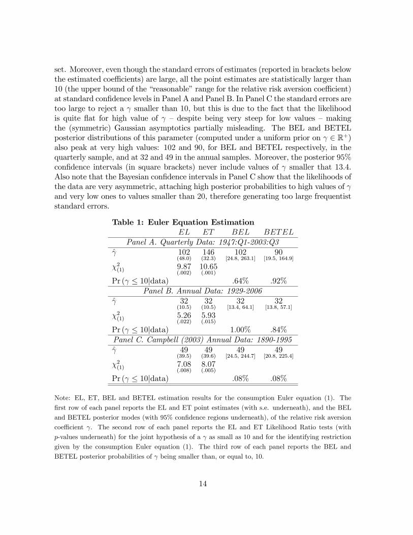
set. Moreover, even though the standard errors of estimates (reported in brackets belowthe estimated coe¢ cients) are large, all the point estimates are statistically larger than10 (the upper bound of the �reasonable�range for the relative risk aversion coe¢ cient)at standard con�dence levels in Panel A and Panel B. In Panel C the standard errors aretoo large to reject a smaller than 10, but this is due to the fact that the likelihoodis quite �at for high value of �despite being very steep for low values �makingthe (symmetric) Gaussian asymptotics partially misleading. The BEL and BETELposterior distributions of this parameter (computed under a uniform prior on 2 R+)also peak at very high values: 102 and 90, for BEL and BETEL respectively, in thequarterly sample, and at 32 and 49 in the annual samples. Moreover, the posterior 95%con�dence intervals (in square brackets) never include values of smaller that 13:4.Also note that the Bayesian con�dence intervals in Panel C show that the likelihoods ofthe data are very asymmetric, attaching high posterior probabilities to high values of and very low ones to values smaller than 20, therefore generating too large frequentiststandard errors.

Table 1: Euler Equation EstimationEL ET BEL BETEL

Panel A. Quarterly Data: 1947:Q1-2003:Q3 102

(48:0)146(32:3)

102[24:8; 263:1]

90[19:5; 164:9]

�2(1) 9:87(:002)

10:65(:001)

Pr ( � 10jdata) :64% :92%Panel B. Annual Data: 1929-2006

32(10:5)

32(10:5)

32[13:4; 64:1]

32[13:8; 57:1]

�2(1) 5:26(:022)

5:93(:015)

Pr ( � 10jdata) 1:00% :84%Panel C. Campbell (2003) Annual Data: 1890-1995 49

(39:5)49(39:6)

49[24:5; 244:7]

49[20:8; 225:4]

�2(1) 7:08(:008)

8:07(:005)

Pr ( � 10jdata) :08% :08%

Note: EL, ET, BEL and BETEL estimation results for the consumption Euler equation (1). The

�rst row of each panel reports the EL and ET point estimates (with s.e. underneath), and the BEL

and BETEL posterior modes (with 95% con�dence regions underneath), of the relative risk aversion

coe¢ cient . The second row of each panel reports the EL and ET Likelihood Ratio tests (with

p-values underneath) for the joint hypothesis of a as small as 10 and for the identifying restriction

given by the consumption Euler equation (1). The third row of each panel reports the BEL and

BETEL posterior probabilities of being smaller than, or equal to, 10.

14

The second row of each panel reports tests for the joint hypothesis of a as smallas 10 and for the identifying restriction given by the consumption Euler equation (1).These tests are the Empirical Likelihood Ratio (ELR) test of Owen (1991, 2001), (inthe �rst column) and the likelihood ratio test proposed in theorem 4 of Kitamura andStutzer (1997). Under the null hypothesis, both statistics follow asymptotically a �2

distribution with one degree of freedom. As revealed by the p-values reported belowthe test statistics, both tests reject the hypothesis of the Euler equation being satis�edby a as small as 10 in all the samples considered.Finally, the third row of each panel reports the posterior probabilities of being

smaller than, or equal to, 10 given the observed data. This probability is small, andnever larger than 1%, for all samples and both BEL and BETEL posteriors.Overall, the results in Table 1 indicate that even adopting an estimation procedure

that allows the probabilities attached to di¤erent states of the economy to di¤er fromtheir sample frequencies, and is therefore robust to rare events problems in the data,the Consumption-CAPM is still rejected and requires a very high level of relative riskaversion to rationalize the stock market risk premium. Moreover, as a robustnesscheck, Table A1 in the Appendix reports estimation and testing results that are robustto violations of the martingale di¤erence property of the conditional Euler equation(that might, for example, be generated by serially correlated measurement error inconsumption as discussed in Wilcox (1992)). This robustness check con�rms the resultsin Table 1.

6 Counterfactual Analysis

�Thus, data are used to calibrate the model economy so that it mimics theworld as closely as possible along a limited, but clearly speci�ed, numberof dimensions.�Kydland and Prescott (1996).

In this section, instead of jointly estimating the coe¢ cient of relative risk aversion andthe probabilities associated with di¤erent states of the economy, we �x the parameterto a �reasonable�value, and ask the ET and EL estimation procedures to identify thedistribution of the data that would solve the Equity Premium Puzzle in the historicalsample. This procedure can be interpreted as calibrating a rare events model (thatsolves the EPP) in a formal �data driven �fashion that minimizes the distance (in theinformation sense) between the model distribution and the true unknown distributionof the data.With this estimated distribution at hand, we can ask the following relevant coun-

terfactual questions. First, suppose that the data were generated by the rare eventsdistribution needed to explain the equity premium puzzle with a low level of risk aver-sion. Under this distribution, what would be the probability of observing an equitypremium puzzle in a sample of the same size as the historical one? That is, if rare

15

events that did not happen frequently enough in the historical sample were the truereason behind the equity premium puzzle, what would be the likelihood of observingsuch a puzzle? Second, suppose rare events were the cause of the equity premiumpuzzle. Would taking these events into account also explain why the C-CAPM per-forms poorly in pricing the cross-section of asset returns? Or would it worsen thecross-sectional failure of the model?In Section 6.1 we present the constructed rare events distribution of the data, while

its implications for the likelihood of observing an equity premium puzzle and for thecross-section of asset returns are discussed, respectively, in Section 6.2 and Section 6.3.

6.1 A World without the Equity Premium Puzzle

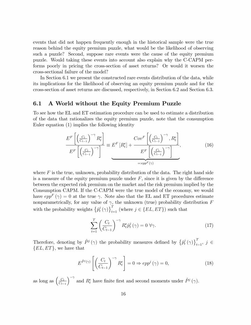
To see how the EL and ET estimation procedure can be used to estimate a distributionof the data that rationalizes the equity premium puzzle, note that the consumptionEuler equation (1) implies the following identity

EF��

CtCt�1

�� Ret

�EF��

CtCt�1

�� � � EF [Ret ] +CovF

��CtCt�1

�� ; Ret

�EF��

CtCt�1

�� �| {z }

=:eppF ( )

; (16)

where F is the true, unknown, probability distribution of the data. The right hand sideis a measure of the equity premium puzzle under F , since it is given by the di¤erencebetween the expected risk premium on the market and the risk premium implied by theConsumption CAPM. If the C-CAPM were the true model of the economy, we wouldhave eppF ( ) = 0 at the true . Note also that the EL and ET procedures estimatenonparametrically, for any value of , the unknown (true) probability distribution F

with the probability weights�pjt ( )

Tt=1

(where j 2 fEL;ETg) such that

TXt=1

�CtCt�1

�� Ret p

jt ( ) = 0 8 . (17)

Therefore, denoting by P j ( ) the probability measures de�ned by�pjt ( )

Tt=1, j 2

fEL;ETg, we have that

EPj( )

"�CtCt�1

�� Ret

#= 0) eppj ( ) = 0, (18)

as long as�

CtCt�1

�� and Ret have �nite �rst and second moments under P

j ( ).

16

That is, �xing the relative risk aversion coe¢ cient , we can use the EL and ETprocedures to construct the probability distribution needed to solve the equity premiumpuzzle. As discussed in Section 3, these procedures are consistent. Moreover, thiscalibration approach minimizes the Kullback-Leibler divergence between the calibrateddistribution and the unknown data generating process. That is, in the same fashionas a Maximum Likelihood estimator, this approach minimizes the distance (in theinformation sense) between the model and the true data generating process. Therefore,this procedure can be interpreted as calibrating a rare events model, that solves theequity premium puzzle, in a rigorous data-driven fashion, since the estimated P j ( ) willbe the closest distribution, among all the distributions that could rationalize the puzzle,to the true unknown data generating process. This implies that, if rare events are thetrue explanation of the equity premium puzzle, the estimated P j ( ), j 2 fEL;ETg,should identify their distribution.In what follows, we discuss the properties and implications of the estimated P j ( )

assuming = 10, that is, a level of relative risk aversion at the upper bound of what iscommonly considered the �reasonable�range for this parameter (e.g. Gollier (2002)).In the Appendix we also report results for = 5.With the P j ( ) estimates at hand, the �rst question to ask is whether the implied

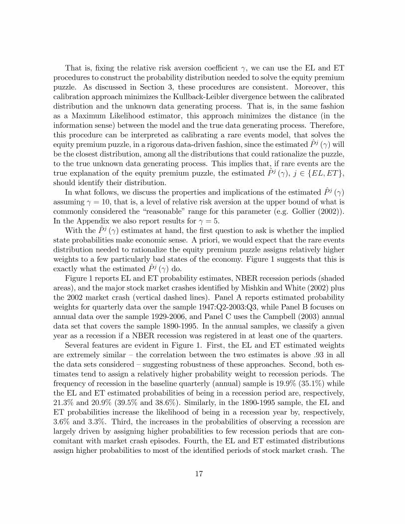
state probabilities make economic sense. A priori, we would expect that the rare eventsdistribution needed to rationalize the equity premium puzzle assigns relatively higherweights to a few particularly bad states of the economy. Figure 1 suggests that this isexactly what the estimated P j ( ) do.Figure 1 reports EL and ET probability estimates, NBER recession periods (shaded

areas), and the major stock market crashes identi�ed by Mishkin andWhite (2002) plusthe 2002 market crash (vertical dashed lines). Panel A reports estimated probabilityweights for quarterly data over the sample 1947:Q2-2003:Q3, while Panel B focuses onannual data over the sample 1929-2006, and Panel C uses the Campbell (2003) annualdata set that covers the sample 1890-1995. In the annual samples, we classify a givenyear as a recession if a NBER recession was registered in at least one of the quarters.Several features are evident in Figure 1. First, the EL and ET estimated weights

are extremely similar �the correlation between the two estimates is above :93 in allthe data sets considered �suggesting robustness of these approaches. Second, both es-timates tend to assign a relatively higher probability weight to recession periods. Thefrequency of recession in the baseline quarterly (annual) sample is 19:9% (35:1%) whilethe EL and ET estimated probabilities of being in a recession period are, respectively,21:3% and 20:9% (39:5% and 38:6%). Similarly, in the 1890-1995 sample, the EL andET probabilities increase the likelihood of being in a recession year by, respectively,3:6% and 3:3%. Third, the increases in the probabilities of observing a recession arelargely driven by assigning higher probabilities to few recession periods that are con-comitant with market crash episodes. Fourth, the EL and ET estimated distributionsassign higher probabilities to most of the identi�ed periods of stock market crash. The

17

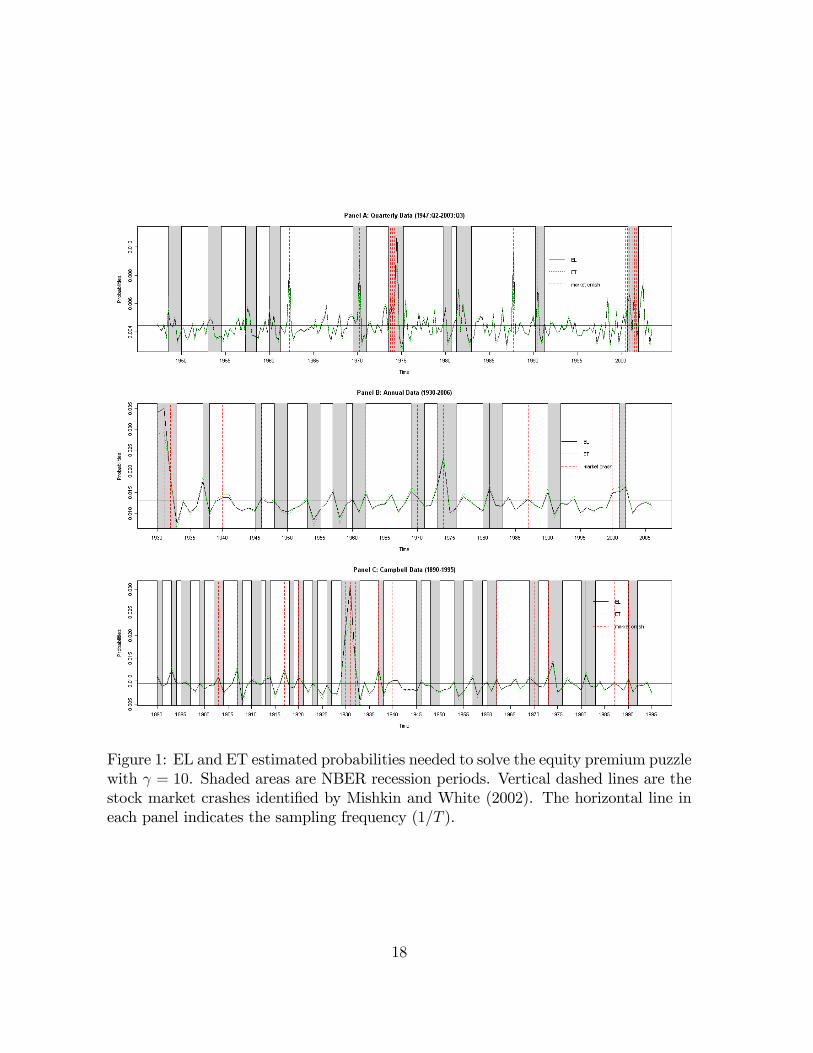
Figure 1: EL and ET estimated probabilities needed to solve the equity premium puzzlewith = 10. Shaded areas are NBER recession periods. Vertical dashed lines are thestock market crashes identi�ed by Mishkin and White (2002). The horizontal line ineach panel indicates the sampling frequency (1=T ).

18

sampling frequency of stock market crashes in the quarterly (annual)27 data is 6:6%(20:8%) while the EL and ET estimated probabilities of a stock market crash are, re-spectively, 10:2% and 9:6% (28:2% and 27:9%). Fifth, the estimated probabilities tendto put the highest weights on few periods characterized by both a stock market crashand a recession �that is, states in which the consumption risk of the stock market isparticularly high, like during the Great Depression period and the 1973-1975 recession.Nevertheless, even the probabilities attached to these states are still fairly small com-pared to the sampling frequency of the observations: for quarterly (annual) data thesampling frequency is :4% (1:3%), while the highest EL and ET probability weightsare, respectively, 1:1% and :9% (3:5% and 2:9%). Similarly, the sampling frequencyin the 1890-1995 sample is :9%, while the highest EL and ET probability weights are,respectivelly, 3:5% and 2:5%.The implications of the estimated probability weights for the distribution of stock

market real returns are summarized in Figure 2. The upper three panels report thehistograms of quarterly (Panel A), annual over the period 1929-2006 (Panel B), andannual over the period 1890-1995 (Panel C), stock market real returns, (Epanechnikov)kernel estimates of the empirical distribution, and weighted (Epanechnikov) kernelestimates, where the weights are given by the estimated P j ( ) probabilities. PanelD (for quarterly data), Panel E (for annual data over the period 1929-2006), andPanel F (for annual data over the period 1890-1995) report the cumulative distributionfunctions of the returns using the empirical weights, and the EL and ET probabilityweights.The �rst thing to notice is that the rare events distribution needed to rationalize

the equity premium puzzle implies thicker negative tails, and a more left skewed dis-tribution than what is obtained using the empirical (sample) weights. Moreover, theEL and ET probability weights generate a leftward shift in the distribution of returnswhen compared with the empirical distribution. This leftward shift implies a reductionin both the median and the mean stock market return: the implied annual median(mean) return is about 4:9%-6:4% (2:1%-5:0%). These numbers are in line with therare events calibrated model of Barro (2006) that �nds an expected risky rate in therange 3:7%-8:4%. One last point worth stressing is that, as shown in Panels D, E, andF of Figure 2, the implied distributions of market returns under PEL ( ) and PET ( )are extremely similar, once again demonstrating robustness of the approach proposed.Rare events models stress that the equity premium puzzle can be rationalized by

assigning higher probabilities to particularly bad states of the economy in which bothmarket returns and consumption growth are low, since these are the states in whichthe consumption risk of the stock market is the highest. Figure 3 shows that this isindeed an implication of the EL and ET estimated probability weights.Each panel of Figure 3 reports the scatter plot of stock market excess returns (hor-

27We classify a given year as a stock market crash year if at least one of the Mishkin and White(2002) crash episodes was recorded.

19

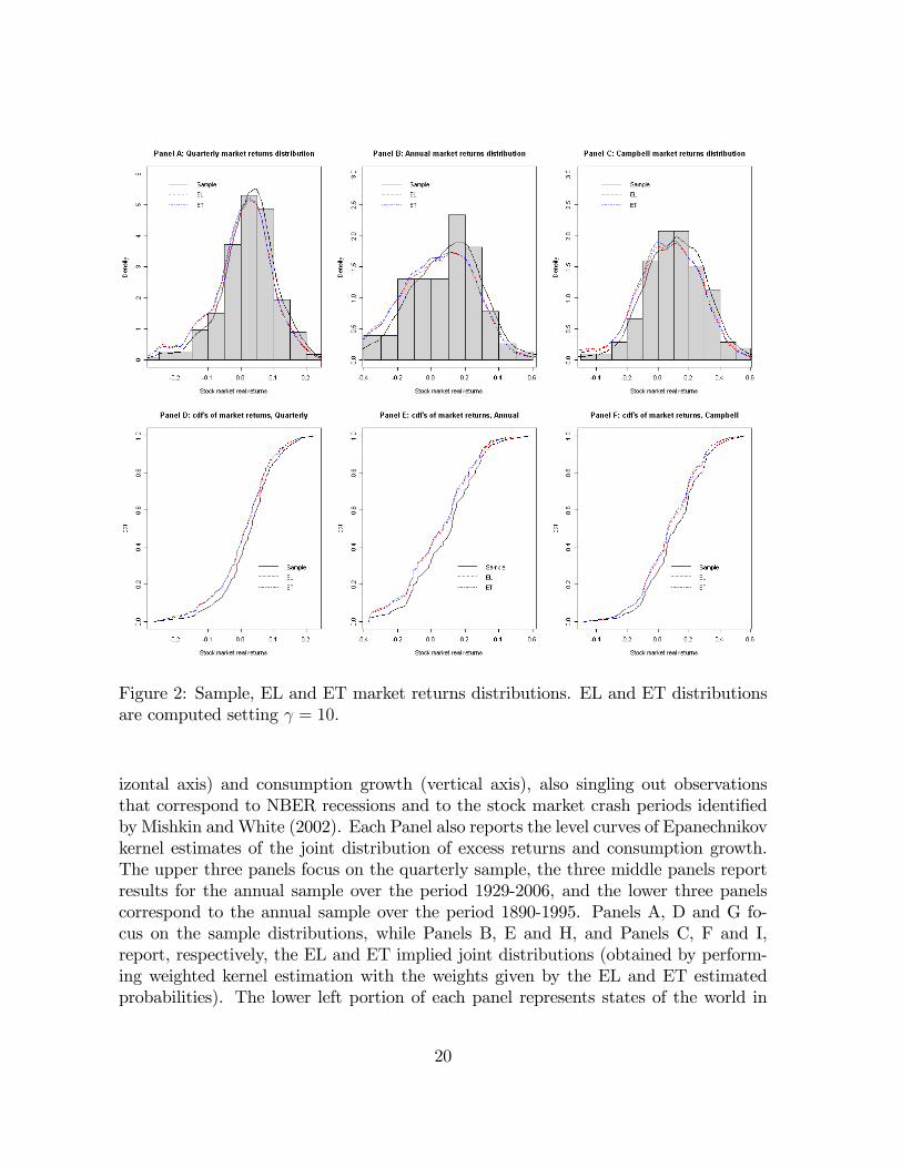
Figure 2: Sample, EL and ET market returns distributions. EL and ET distributionsare computed setting = 10.

izontal axis) and consumption growth (vertical axis), also singling out observationsthat correspond to NBER recessions and to the stock market crash periods identi�edby Mishkin andWhite (2002). Each Panel also reports the level curves of Epanechnikovkernel estimates of the joint distribution of excess returns and consumption growth.The upper three panels focus on the quarterly sample, the three middle panels reportresults for the annual sample over the period 1929-2006, and the lower three panelscorrespond to the annual sample over the period 1890-1995. Panels A, D and G fo-cus on the sample distributions, while Panels B, E and H, and Panels C, F and I,report, respectively, the EL and ET implied joint distributions (obtained by perform-ing weighted kernel estimation with the weights given by the EL and ET estimatedprobabilities). The lower left portion of each panel represents states of the world in

20

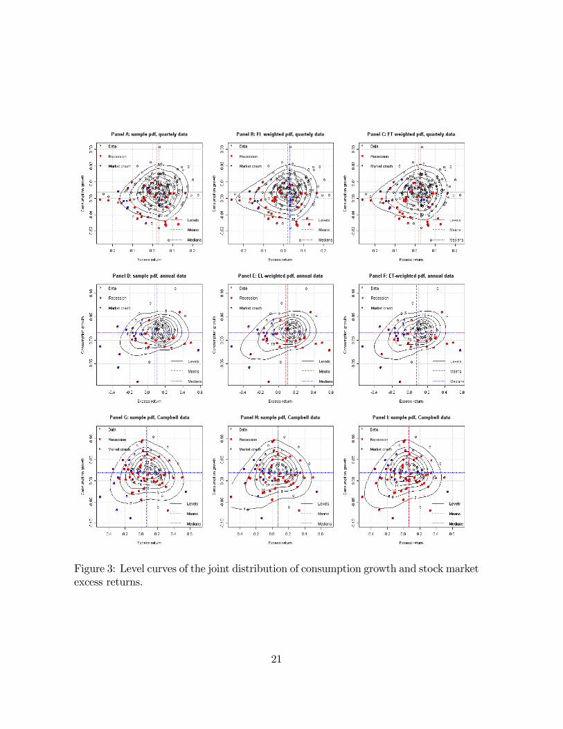
Figure 3: Level curves of the joint distribution of consumption growth and stock marketexcess returns.

21

which the consumption risk of the stock market is highest, i.e. observations that arecharacterized by both low excess returns and low consumption growth. Not surpris-ingly, this is also the area were recessions and stock market crashes tend to appearmore often. Comparing the level curves in Panels A, D and G with the ones in theother panels, it appears clearly that the EL and ET probability weights skew the jointdistribution of consumption growth and market returns toward the lower left portionof the graphs, thereby increasing the likelihood of high stock market consumption riskstates. Moreover, most of the shift in probability mass happens on the lowest levelcurve i.e., in the tail of the joint distribution, as the rare events explanation of theequity premium puzzle would imply.

Overall, the results of this section suggest that using the EL and ET approachesto construct distributions of the data that rationalize the equity premium puzzle witha low level of risk aversion, and that are at the same time as close as possible tothe true unknown distribution of the data, deliver results that are: a) robust, sinceboth approaches have extremely similar implications, and b) in line with what the rareevents hypothesis predicts should be the mechanisms needed to rationalize the equitypremium puzzle.In the next two sections, we ask whether a rare events model characterized by

the P j ( ) probability weights discussed above a) would be likely to deliver an equitypremium puzzle of the same magnitude as the historical one in a sample of the samelength as the historical one, and b) can help explain the inability of the standardConsumption CAPM to price the cross-section of asset returns.

6.2 How likely is the Equity Premium Puzzle?

The P j ( ), j 2 fEL;ETg, measures just discussed provide the most probable (in thelikelihood sense) rare events explanation of the equity premium puzzle. But underthese measures, what is the likelihood of observing an equity premium puzzle in asample of the same size as the historical one?To answer this question we perform the following counterfactual exercise. First,

we use the estimated P j ( ), j 2 fEL;ETg, distributions to generate counterfac-tual samples of data of the same size as the historical ones. That is, we use the�pjt ( )

Tt=1, j 2 fEL;ETg, probabilities to draw with replacement from the observed

datan

CtCt�1

;Ret

oTt=1, and use these draws to form samples of size T . We generate a

total of 100; 000 counterfactual samples in this fashion (for both quarterly and annualdata).Second, in each sample i we compute the realized equity premium puzzle, eppTi ( ),

22

as

eppTi ( ) = ET�Rei;t�+

CovT��

Ci;tCi;t�1

�� ; Rei;t

�ET��

Ci;tCi;t�1

�� � (19)

where ET [:] and CovT [:] denote the sample moment operators, and is �xed to thesame low level used to construct P j ( ). Moreover, in each generated sample we performa GMM estimation of the coe¢ cient of relative risk aversion.The results of this counterfactual exercise are summarized in Table 2. The �rst

column reports the equity premium puzzle, as a function of , in the historical samples.The second column reports the median and, in squared brackets, the 95% con�denceinterval of the realized equity premium puzzle in the counterfactual samples. The thirdcolumn reports the probability of observing, in the counterfactual samples, a realizedequity premium puzzle at least as large as the historical one. The last column reportsthe median and, in squared brackets, the 95% con�dence interval of the estimated coe¢ cient in the counterfactual samples. Panel A focuses on quarterly data, whilePanels B and C hinge upon annual observations over the periods 1929-2006 and 1890-1995, respectively. Quarterly rates in Panel A are annualized for the sake of comparisonwith the annual ones in Panels B and C.The �rst row, �rst column, of Panel A shows that the assumption of a relative risk

aversion coe¢ cient of 5 implies, in the 1947:Q2-2003:Q3 sample, an equity premiumpuzzle of 7:4% per year. The second column shows instead that the median realizedequity premium puzzle in the counterfactual samples generated by the EL probabili-ties with = 5 is 0%, and that the upper bound of its 95% con�dence band is only4:7% �that is, the con�dence interval does not include the historically observed eq-uity premium puzzle.28 Moreover, in the counterfactual samples, a negative realizedequity premium puzzle seems almost as likely as a positive one. This is due to thefact that increasing the probabilities attached to extremely bad states of the economymakes it more likely to observe too many of these events in a �nite sample, thereforeincreasing the likelihood of observing a negative equity premium puzzle in the counter-factual samples. The third column shows that, for a risk aversion of 5, the likelihoodof observing an equity premium puzzle at least as large as the historical one wouldbe extremely low �about 0:10%. The last column reports the median estimate andthe 95% con�dence bands, in square brackets, of the estimated relative risk aversioncoe¢ cient.29 The estimates are centered around the true value used to generate thesamples, but the 95% interval is very large, ranging from �41 to 67. This �nding is inline with the evidence of poor performance of the GMM estimator in the presence ofrare events (Saikkonnen and Ripatti (2000)).

28Median and con�dence bands are computed from the percentiles of�eppTi ( )

100;000i=1

:29Median and con�dence bands are computed from the percentiles of

� i;GMM

100;000i=1

.

23

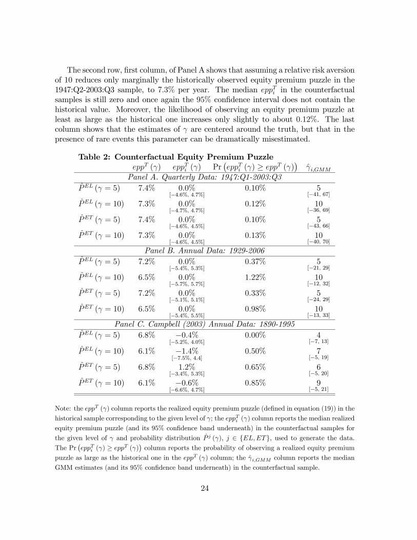
The second row, �rst column, of Panel A shows that assuming a relative risk aversionof 10 reduces only marginally the historically observed equity premium puzzle in the1947:Q2-2003:Q3 sample, to 7:3% per year. The median eppTi in the counterfactualsamples is still zero and once again the 95% con�dence interval does not contain thehistorical value. Moreover, the likelihood of observing an equity premium puzzle atleast as large as the historical one increases only slightly to about 0:12%. The lastcolumn shows that the estimates of are centered around the truth, but that in thepresence of rare events this parameter can be dramatically misestimated.

Table 2: Counterfactual Equity Premium PuzzleeppT ( ) eppTi ( ) Pr

�eppTi ( ) � eppT ( )

� i;GMM

Panel A. Quarterly Data: 1947:Q1-2003:Q3PEL ( = 5) 7:4% 0:0%

[�4:6%, 4:7%]0:10% 5

[�41, 67]

PEL ( = 10) 7:3% 0:0%[�4:7%, 4:7%]

0:12% 10[�36, 69]

PET ( = 5) 7:4% 0:0%[�4:6%, 4:5%]

0:10% 5[�43, 66]

PET ( = 10) 7:3% 0:0%[�4:6%, 4:5%]

0:13% 10[�40, 70]

Panel B. Annual Data: 1929-2006PEL ( = 5) 7:2% 0:0%

[�5:4%, 5:3%]0:37% 5

[�21, 29]

PEL ( = 10) 6:5% 0:0%[�5:7%, 5:7%]

1:22% 10[�12, 32]

PET ( = 5) 7:2% 0:0%[�5:1%, 5:1%]

0:33% 5[�24, 29]

PET ( = 10) 6:5% 0:0%[�5:4%, 5:5%]

0:98% 10[�13, 33]

Panel C. Campbell (2003) Annual Data: 1890-1995PEL ( = 5) 6:8% �0:4%

[�5:2%, 4:0%]0:00% 4

[�7, 13]

PEL ( = 10) 6:1% �1:4%[�7:5%, 4:4]

0:50% 7[�5, 19]

PET ( = 5) 6:8% 1:2%[�3:4%, 5:3%]

0:65% 6[�5, 20]

PET ( = 10) 6:1% �0:6%[�6:6%, 4:7%]

0:85% 9[�5, 21]

Note: the eppT ( ) column reports the realized equity premium puzzle (de�ned in equation (19)) in the

historical sample corresponding to the given level of ; the eppTi ( ) column reports the median realized

equity premium puzzle (and its 95% con�dence band underneath) in the counterfactual samples for

the given level of and probability distribution P j ( ), j 2 fEL;ETg, used to generate the data.The Pr

�eppTi ( ) � eppT ( )

�column reports the probability of observing a realized equity premium

puzzle as large as the historical one in the eppT ( ) column; the i;GMM column reports the median

GMM estimates (and its 95% con�dence band underneath) in the counterfactual sample.

24

The last two rows of Panel A of Table 2 use the ET probabilities instead of the ELones. The results are largely in line with the ones in the �rst two rows: the medianequity premium puzzle in the counterfactual samples is zero and its 95% con�dencebands are too tight to include the historical values. Moreover, the historical equitypremium puzzle is very unlikely to arise: its probability is at most 0:13%.Panel B of Table 2 reports the same exercise as in Panel A, but it uses annual

observations over the sample 1929-2006. The median eppTi is about zero for both ELand ET probabilities and, irrespective of the value of considered, the 95% con�dencebands do not include the historical values of the puzzle. Most importantly, even inthis sample the probability of observing an equity premium puzzle of at least the samemagnitude as the historical one is extremely small, ranging from 0:33% to 1:22%. Onceagain, the GMM estimates of are centered around the truth but the con�dence bandstend to be very large, suggesting that in the presence of rare events the risk aversioncoe¢ cient is likely to be misestimated.Panel C reports the results for the annual sample over the period 1890-1995. The

results are largely similar to those in Panels A and B. The median eppTi across coun-terfactual samples is negative in three out of the four cases and the 95% con�denceintervals do not include the historically observed equity premium puzzle. Moreover,an equity premium puzzle of at least the same magnitude as the historical one is veryunlikely to arise in a sample of the same length as the historical one. Finally, theGMM estimates of are centered around the truth and the con�dence intervals aremuch tighter than those in Panel B, re�ecting the larger sample size in the latter Panel.As a robustness check, in the Appendix we present a similar counterfactual ex-

ercise that is robust to potential violations of the martingale di¤erence property ofthe conditional consumption Euler equation. This approach, combined with a simplemodi�cation of the procedure for drawing counterfactual samples (presented in SectionA.1.4), also allows us to preserve the autocorrelation properties of consumption growthand returns. As shown by Table A2 in the Appendix, this robustness check con�rmsthe results in Table 2.

Overall, the results presented in this section imply that if the data were generatedby the rare events distribution needed to rationalize the equity premium puzzle, thepuzzle itself would be very unlikely to arise in samples of the same size as the historicalones. This suggests that if one is willing to believe that the rare events hypothesis isthe explanation of the equity premium puzzle, one should also believe that the puzzleitself is a rare event.

6.3 Rare events and the cross-section of asset returns

Having identi�ed the EL and ET probability weights needed to rationalize the equitypremium puzzle with a low level of risk aversion, we can explore whether rare events

25

are a viable explanation of the poor performance of the C-CAPM in pricing the cross-section of asset returns.The consumption Euler equation implies that the expected excess return on any

asset should be fully explained by the asset�s consumption risk, where the latter ismeasured by the covariance of the excess return with the ratio of marginal utilitiesbetween two consecutive periods. That is, for any asset m with associated excessreturn Rem;t, and denoting with F the true distribution of the data, we have that thefollowing relation

EF�Rem;t

�= ��

CovF��

CtCt�1

�� ; Rem;t

�EF��

CtCt�1

�� �| {z }

=:�m

� (20)

should hold exactly (at the true ) with � = 0 and � = 1. Similarly, linearizing thepricing kernel to get rid of (see e.g. Parker and Julliard (2003)), we have that thefollowing relation

EF�Rem;t

�= �+ CovF

�ln

CtCt�1

; Rem;t

�| {z }

=:�m

� (21)

should hold with � = 0 and � > 0. The �m terms in equations (20) and (21) can beinterpreted as a measure of the consumption risk that an agent undertakes investingin asset m.It is a well documented empirical regularity that the above implications of the C-

CAPM are rejected by the data when the moments in equations (20) and (21) arereplaced with their sample analogs (see e.g. Mankiw and Shapiro (1986), Breeden,Gibbons, and Litzenberger (1989), Campbell (1996), Cochrane (1996), Lettau andLudvigson (2001), Parker and Julliard (2005)). Nevertheless, if the empirical failuresof the C-CAPM were the outcome of rare events that happened to occur with too lowfrequency in the historical sample, we would expect equations (20) and (21) to hold ifthe moments were constructed taking explicitly these rare events into account. That is,using the probability weights P j ( ), j 2 fEL;ETg, needed to rationalize the equitypremium puzzle under the rare events hypothesis (and presented in Section 6.1), wewould expect

EPj( )�Rem;t

�= ��

CovPj( )

��CtCt�1

�� ; Rem;t

�EP j( )

��CtCt�1

�� � �, (22)

26

to hold with � = 0 and � = 1, and

EPj( )�Rem;t

�= �+ CovP

j( )

�ln

CtCt�1

; Rem;t

�� (23)

to hold with � = 0 and � > 0.To test this hypothesis we use the quarterly cross-section of Fama-French 25 port-

folios and construct excess returns as these returns less the return on the 3-monthTreasury Bill rate. To obtain empirical estimates of � and �, we use the two-stepFama and MacBeth (1973) cross-sectional regression procedure, adapted to take intoaccount that the moments in equations (22) and (23) should be constructed under theP j ( ) probability measures rather than as sample analogs. The EL and ET probabil-ity weights (P j ( )) are the ones described in Section 6.1 under the assumption that = 10, and we therefore estimate equation (22) setting = 10 in the pricing kernel.The point estimate of � measures the extent by which the model fails to price theaverage equity premium in the cross-section of the Fama and French (1992) 25 portfo-lios. The estimation procedure is described in detail in Appendix A.2. Cross-sectionalestimation results are reported in Table 3.The �rst column of the table reports the cross-sectional R2 for all the models

considered.30 The second and third columns report, respectively, the point estimatesof � and � and their standard errors (in parentheses). In order to disentangle thechannels through which the rare events distributions P j ( ) a¤ect the cross-sectionalperformance of the C-CAPM, Table 3 also reports two additional statistics. The fourthcolumn reports the percentage change in the ratio of the cross-sectional variance ofconsumption risk measures to the cross-sectional variance of average excess returns(that is V ar (�m) =V ar

�E�Rem;t+1

��) caused by using the P j ( ) probability weights,

instead of sample averages, in computing the moments in equations (22) and (23).The �fth column reports the change in the cross-sectional variance of the correlationsbetween the pricing kernel and excess returns in equations (22) and (23), that is thechange in V ar (�m), where �m is de�ned as

�m := corr

�CtCt�1

�� ; Rem;t

!(24)

for the non-linear representation in equation (20), and as

�m := corr

�ln

CtCt�1

; Rem;t

�(25)

for the linearized case in equation (21). Panel A of Table 3 focuses on the estimationof equations (20) and (22), while Panel B reports the estimation results of equations(21) and (23).

30Details on how to construct this statistic under the P j ( ) probability measures are reported inAppendix A.2.

27

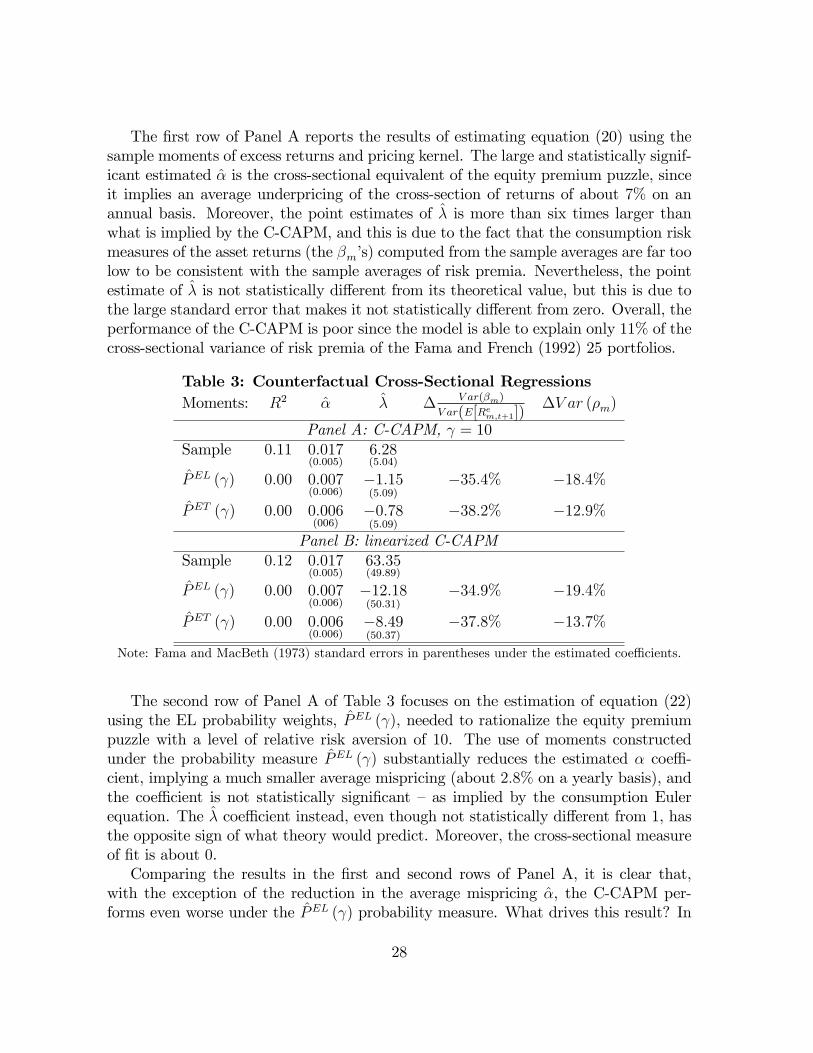
The �rst row of Panel A reports the results of estimating equation (20) using thesample moments of excess returns and pricing kernel. The large and statistically signif-icant estimated � is the cross-sectional equivalent of the equity premium puzzle, sinceit implies an average underpricing of the cross-section of returns of about 7% on anannual basis. Moreover, the point estimates of � is more than six times larger thanwhat is implied by the C-CAPM, and this is due to the fact that the consumption riskmeasures of the asset returns (the �m�s) computed from the sample averages are far toolow to be consistent with the sample averages of risk premia. Nevertheless, the pointestimate of � is not statistically di¤erent from its theoretical value, but this is due tothe large standard error that makes it not statistically di¤erent from zero. Overall, theperformance of the C-CAPM is poor since the model is able to explain only 11% of thecross-sectional variance of risk premia of the Fama and French (1992) 25 portfolios.

Table 3: Counterfactual Cross-Sectional RegressionsMoments: R2 � � � V ar(�m)

V ar(E[Rem;t+1])�V ar (�m)

Panel A: C-CAPM, = 10Sample 0:11 0:017

(0:005)6:28(5:04)

PEL ( ) 0:00 0:007(0:006)

�1:15(5:09)

�35:4% �18:4%

PET ( ) 0:00 0:006(006)

�0:78(5:09)

�38:2% �12:9%

Panel B: linearized C-CAPMSample 0:12 0:017

(0:005)63:35(49:89)

PEL ( ) 0:00 0:007(0:006)

�12:18(50:31)

�34:9% �19:4%

PET ( ) 0:00 0:006(0:006)

�8:49(50:37)

�37:8% �13:7%

Note: Fama and MacBeth (1973) standard errors in parentheses under the estimated coe¢ cients.

The second row of Panel A of Table 3 focuses on the estimation of equation (22)using the EL probability weights, PEL ( ), needed to rationalize the equity premiumpuzzle with a level of relative risk aversion of 10. The use of moments constructedunder the probability measure PEL ( ) substantially reduces the estimated � coe¢ -cient, implying a much smaller average mispricing (about 2:8% on a yearly basis), andthe coe¢ cient is not statistically signi�cant � as implied by the consumption Eulerequation. The � coe¢ cient instead, even though not statistically di¤erent from 1, hasthe opposite sign of what theory would predict. Moreover, the cross-sectional measureof �t is about 0.Comparing the results in the �rst and second rows of Panel A, it is clear that,

with the exception of the reduction in the average mispricing �, the C-CAPM per-forms even worse under the PEL ( ) probability measure. What drives this result? In

28

order to increase the ability of the C-CAPM to price the cross-section of returns, thePEL ( ) empirical measure should in principle increase the cross-sectional variance ofconsumption risk, V ar (�m), relative to the cross-sectional variance of average risk pre-mia, V ar

�E�Rem;t

��. But the entry on column four, second row, of Panel A shows that

the exact opposite happens: moving from sample moments to the PEL ( ) weightedmoments, V ar (�m) =V ar

�E�Rem;t

��is reduced by about 35:4%. And, as shown by the

�fth column of the same row, this is due to the fact that the cross-sectional variationof the correlation between the pricing kernel and excess returns, V ar (�m), is reducedby about 18:4% using the PEL ( ) weights. This last �nding is a direct consequenceof the rare events explanation of the equity premium puzzle. In order to rationalizethe equity premium puzzle with a low level of risk aversion, we need to assign higherprobability to bad �economy wide �states such as deep recessions and market crashes.But in a market crash or a deep recession all the assets in the cross-section tends toyield low returns and consumption growth tend to be lower. Therefore, increasing theprobability of these type of states has two e¤ects. On one hand, it can rationalize theaverage risk premium on the market since, at the same time, it increase the consump-tion risk of investing in �nancial assets and reduces the expected returns. On the otherhand, it makes it harder to explain the cross-section of risk premia, since it reduces thecross-sectional variability of consumption risk across assets.The third row of Panel A of Table 3 uses the PET ( ) probability weights for the

estimation of equation (22). The results are very similar to the ones obtained usingthe PEL ( ) weights: the model �ts better the average risk premium but its abilityto explain the cross-section of returns is reduced due to the substantial reduction inboth V ar (�m) =V ar

�E�Rem;t+1

��and in the cross-sectional variation of the correlation

between the pricing kernel and excess returns, V ar(�m).Panel B of Table 3 focuses on the cross-sectional estimation of the C-CAPM in

its linearized form reported in equations (21) and (23). The advantage of using thelinearized approach is that the results do not depend on the choice of a pre-speci�edlevel for the relative risk aversion parameter . The �rst row of Panel B uses the sam-ple moments of returns and consumption growth and reproduces the standard poorperformance of the C-CAPM in explaining the cross-section of asset returns (see e.g.Parker and Julliard (2003)): the model is able to explain only 12% of the cross-sectionalvariation of average excess returns; the large � estimate is statistically signi�cant andimplies an average underpricing close to 7% on an annual basis; � has the right signbut is not statistically di¤erent from zero. The second and third rows focus, respec-tively, on the implications of using the PEL ( ) and PET ( ) weights in estimating themoments in equation (23). The results are substantially in line with the ones reportedin Panel A. Using the P j ( ) probability weights helps the C-CAPM �t better the av-erage risk premium on the market but it worsens the ability of the model to explainthe cross-sectional di¤erences in average returns. This is due to the reduction in thecross-sectional variation of consumption risk caused by attaching higher probability to

29

infrequent, economy wide, bad states during which consumption growth is low and allthe assets tend to perform poorly.Overall, the estimates in Table 3 suggest that the rare events explanation of the

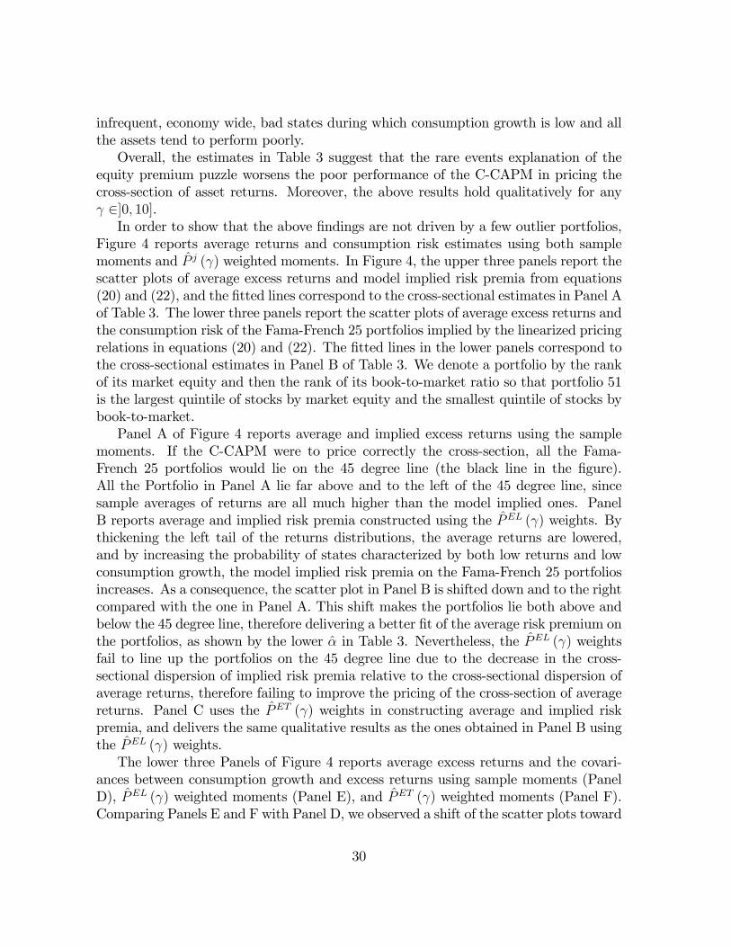
equity premium puzzle worsens the poor performance of the C-CAPM in pricing thecross-section of asset returns. Moreover, the above results hold qualitatively for any 2]0; 10].In order to show that the above �ndings are not driven by a few outlier portfolios,

Figure 4 reports average returns and consumption risk estimates using both samplemoments and P j ( ) weighted moments. In Figure 4, the upper three panels report thescatter plots of average excess returns and model implied risk premia from equations(20) and (22), and the �tted lines correspond to the cross-sectional estimates in Panel Aof Table 3. The lower three panels report the scatter plots of average excess returns andthe consumption risk of the Fama-French 25 portfolios implied by the linearized pricingrelations in equations (20) and (22). The �tted lines in the lower panels correspond tothe cross-sectional estimates in Panel B of Table 3. We denote a portfolio by the rankof its market equity and then the rank of its book-to-market ratio so that portfolio 51is the largest quintile of stocks by market equity and the smallest quintile of stocks bybook-to-market.Panel A of Figure 4 reports average and implied excess returns using the sample

moments. If the C-CAPM were to price correctly the cross-section, all the Fama-French 25 portfolios would lie on the 45 degree line (the black line in the �gure).All the Portfolio in Panel A lie far above and to the left of the 45 degree line, sincesample averages of returns are all much higher than the model implied ones. PanelB reports average and implied risk premia constructed using the PEL ( ) weights. Bythickening the left tail of the returns distributions, the average returns are lowered,and by increasing the probability of states characterized by both low returns and lowconsumption growth, the model implied risk premia on the Fama-French 25 portfoliosincreases. As a consequence, the scatter plot in Panel B is shifted down and to the rightcompared with the one in Panel A. This shift makes the portfolios lie both above andbelow the 45 degree line, therefore delivering a better �t of the average risk premium onthe portfolios, as shown by the lower � in Table 3. Nevertheless, the PEL ( ) weightsfail to line up the portfolios on the 45 degree line due to the decrease in the cross-sectional dispersion of implied risk premia relative to the cross-sectional dispersion ofaverage returns, therefore failing to improve the pricing of the cross-section of averagereturns. Panel C uses the PET ( ) weights in constructing average and implied riskpremia, and delivers the same qualitative results as the ones obtained in Panel B usingthe PEL ( ) weights.The lower three Panels of Figure 4 reports average excess returns and the covari-

ances between consumption growth and excess returns using sample moments (PanelD), PEL ( ) weighted moments (Panel E), and PET ( ) weighted moments (Panel F).Comparing Panels E and F with Panel D, we observed a shift of the scatter plots toward

30

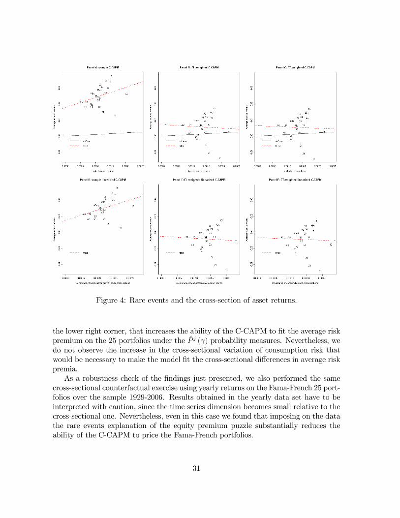
Figure 4: Rare events and the cross-section of asset returns.

the lower right corner, that increases the ability of the C-CAPM to �t the average riskpremium on the 25 portfolios under the P j ( ) probability measures. Nevertheless, wedo not observe the increase in the cross-sectional variation of consumption risk thatwould be necessary to make the model �t the cross-sectional di¤erences in average riskpremia.As a robustness check of the �ndings just presented, we also performed the same

cross-sectional counterfactual exercise using yearly returns on the Fama-French 25 port-folios over the sample 1929-2006. Results obtained in the yearly data set have to beinterpreted with caution, since the time series dimension becomes small relative to thecross-sectional one. Nevertheless, even in this case we found that imposing on the datathe rare events explanation of the equity premium puzzle substantially reduces theability of the C-CAPM to price the Fama-French portfolios.

31

Overall, the results of this section suggest that forcing on the data the rare eventsrationalization of the equity premium puzzle would worsen the already poor perfor-mance of the C-CAPM in pricing the cross-section of asset returns. This �nding isdriven by the fact that, in order to rationalize the equity premium puzzle with a lowlevel of risk aversion, we need to assign higher probability to bad �economy wide �states such as recessions and market crashes. Since during market crashes and deeprecessions all the assets in the cross-section tend to yield low returns and consump-tion growth tends to be low, this reduces the cross-sectional variability of consumptionrisk across assets, making it harder for the model to explain the cross-section of riskpremia. This �nding also suggests that explanations of the equity premium puzzlebased on agents�expectations of an economy wide disaster (e.g. a �nancial marketmeltdown) that has not materialized in the sample �a so called peso phenomenon �would also reduce the ability of the Consumption-CAPM to price the cross-section ofasset returns, since such an expectation would reduce the cross-sectional dispersion ofconsumption risk across assets.

7 Rationalizing the Discrepancy with Barro (2006)

The results presented in the previous sections suggest that the rare events hypothesisis an unlikely explanation of the equity premium puzzle. This conclusion is partiallyin contrast with the calibration evidence in Barro (2006) that �nds strong supportfor the rare events hypothesis. In this section we investigate the reasons behind thisdiscrepancy.The key element in Barro (2006) is the calibration of the consumption contraction

during a rare economic disaster. In order to identify a reasonable value for this quantity,Barro performs an extensive study of the major economic disasters of the twentiethcentury in a cross section of 35 countries (the data are taken from Maddison (2003)).The criterion he uses to identify an economic disaster is a cumulated multi-year dropin GDP per capita of more than 15%. Based on these identi�ed disasters, he calibratesthe distribution of the one-year consumption drop during a disaster as being equalto the empirical distribution of multi-year GDP drop in the cross-country sample ofdisasters.This calibration choice raises two concerns. First, if the identi�ed disasters tend to

last for more than one year, this approach overstates the degree of consumption risk,since a risk averse agent fears one large contraction in consumption more than havingthe same shock spread over several years. Second, if agents are able to at least partiallysmooth income shocks over time, we would expect consumption to drop by less thanGDP during disasters.Indeed, both concerns seem to be supported by the data. Figure 5 plots the his-

togram of annualized GDP contractions in the 60 rare disasters considered in Barro

32

(2006). The �rst things to notice are that a) all but two out of the 60 disasters arecharacterized by an annualized contraction smaller than Barro�s (average) calibratedvalue of 29% (black continuous line), b) the median annualized contraction (red dashedline) is less than a quarter of that value (being about 7%), and c) Barro�s averagecalibrated value is extreme �and rare �even among rare events, since it lies on the farright tail of the distribution of annualized disasters. These �ndings are not surprisingsince most of the twentieth century disaster episodes lasted several years �the averagetime length is about four years, and 59 out of 60 disasters lasted more than one year.

Figure 5: Histogram of annualized GDP contractions during the 60 major economicdisasters of the Twentieth Century. Source: Barro (2006), Table I, and authors�calcu-lations.

The �gure also singles out the cumulated contractions in GDP (green dotted line)and consumption (blue dash-dotted line) during the U.S. Great Depression. What isstriking is that the contraction in consumption (17%) is close to half the GDP drop(31%). Moreover, the U.S. Great Depression cumulated contraction in consumption isabout 12% lower than Barro�s average calibrated value �even though the U.S. GreatDepression cumulated contraction in GDP (31%) is above the average cumulated GDPcontraction during disasters (this being 29%). That is, even in a country characterizedby a larger than average economic disaster, the cumulated contraction in consumptionis much smaller than Barro�s (average) calibrated value.

33

The above observations do not per se rationalize the discrepancy between the resultspresented in the previous sections and those in Barro (2006). We now address this issueformally. In order to do so, we perform the following counterfactual exercise.First, we modify our baseline annual data sample (1929-2006) by replacing the four

data points corresponding to the Great Depression period with one calibrated disasterobservation. In order to assess the e¤ect of Barro�s calibration approach, we calibratethe rare disaster observation in two ways: �rst as the cumulated consumption dropduring the U.S. Great Depression, and second as the cumulated GDP drop during thesame period. If these two assumptions were the reason behind the discrepancy betweenour results and Barro�s ones, we would expect that a) using the cumulated consumptiondrop the estimated risk aversion parameter should be smaller than the one in PanelB of Table 1 (namelly, 32), and that b) using the cumulated contraction in GDP, weshould �nd an even lower risk aversion coe¢ cient and a high likelihood of having theEuler equation satis�ed with a relative risk aversion smaller than 10. In both modi�edsamples, the market return during the disaster is calibrated to match the annualizedexcess return during the great derpression.Second, we use these modi�ed samples to estimate and test the consumption Euler

equation (1). The estimation is performed, as in Section 5, using a set of estimatorsthat are robust to rare events problems in the data, since they allow the probabilitiesattached to di¤erent states of the economy to di¤er from their sample frequencies.Moreover, using the calibration and simulation procedures of Section 6.2, we elicit thelikelihood of observing an Equity Premium Puzzle if the data were generated by therare events probability distribution needed to rationalize the puzzle with a low level ofrisk aversion.We undertake this counterfactual exercise �that uses a mix of real and �ctitious

data �in order to perform a controlled experiment, since we know from Table 1 andTable 2 that in the true 1929-2006 sample i) the Consumption-CAPM is rejected andrequires a high level of relative risk aversion (32) to rationalize the stock market riskpremium, and that ii) if the data were generated by the rare events distribution neededto rationalize the equity premium puzzle, the puzzle itself would be very unlikely toarise in a sample of the same size as the historical one. This counterfactual exercise ispresented in Table 4.Panel A of Table 4 calibrates the economic disaster to match the cumulative con-

sumption drop during the U.S. Great Depression, while Panel B uses the cumulativeGDP contraction during the same period. The �rst row of each panel reports the ELand ET point estimates (with standard errors in parenthesis), as well as the BEL andBETEL posterior modes (with 95% con�dence regions in brackets), of the relative riskaversion coe¢ cient . The second row of each panel reports the EL and ET LikelihoodRatio tests (with p-values in parenthesis) for the joint hypothesis of a as small as 10and for the identifying restriction given by the consumption Euler equation (1). Thethird row of each panel reports the BEL and BETEL posterior probabilities of being

34

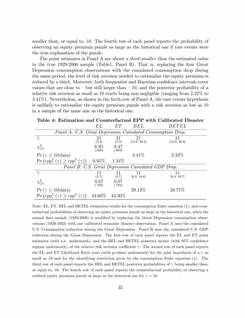
smaller than, or equal to, 10. The fourth row of each panel reports the probability ofobserving an equity premium puzzle as large as the historical one if rare events werethe true explanation of the puzzle.The point estimates in Panel A are about a third smaller than the estimated value

in the true 1929-2006 sample (Table1, Panel B). That is, replacing the four GreatDepression consumption observations with the cumulated consumption drop duringthe same period, the level of risk aversion needed to rationalize the equity premium isreduced by a third. Moreover, both frequentist and Bayesian con�dence intervals covervalues that are close to �but still larger than �10, and the posterior probability of arelative risk aversion as small as 10 starts being non negligible (ranging from 2:32% to3:41%). Nevertheless, as shown in the forth row of Panel A, the rare events hypothesisis unlikely to rationalize the equity premium puzzle with a risk aversion as low as 10in a sample of the same size as the historical one.

Table 4: Estimation and Counterfactual EPP with Calibrated DisasterEL ET BEL BETEL

Panel A. U.S. Great Depression Cumulated Consumption Drop. 21

(5:3)21(5:3)

21[12:6; 39:4]

21[12:9; 38:9]

�2(1) 6:95(:008)

8:47(:003)

Pr ( � 10jdata) 3:41% 2:32%Pr�eppTi ( ) � eppT ( )

�0:95% 1:34%

Panel B. U.S. Great Depression Cumulated GDP Drop. 11

(2:7)11(2:7)

11[6:3; 19:8]

11[6:4; 19:7]

�2(1) 0:07(:792)

0:07(:784)

Pr ( � 10jdata) 29:13% 28:71%Pr�eppTi ( ) � eppT ( )

�43:60% 43:30%

Note: EL, ET, BEL and BETEL estimation results for the consumption Euler equation (1), and coun-

terfactual probabilities of observing an equity premium puzzle as large as the historical one, when the

annual data sample (1929-2006) is modi�ed by replacing the Great Depression consumption obser-

vations (1929-1933) with one calibrated economic disaster observation. Panel A uses the cumulated

U.S. Consumption reduction during the Great Depression. Panel B uses the cumulated U.S. GDP

reduction during the Great Depression. The �rst row of each panel reports the EL and ET point

estimates (with s.e. underneath), and the BEL and BETEL posterior modes (with 95% con�dence

regions underneath), of the relative risk aversion coe¢ cient . The second row of each panel reports

the EL and ET Likelihood Ratio tests (with p-values underneath) for the joint hypothesis of a as

small as 10 and for the identifying restriction given by the consumption Euler equation (1). The

third row of each panel reports the BEL and BETEL posterior probabilities of being smaller than,

or equal to, 10. The fourth row of each panel reports the counterfactual probability of observing a

realized equity premium puzzle as large as the historical one for = 10.

35

In Panel B we calibrate the consumption drop during the disaster to the same valueas the cumulated GDP drop during the U.S. Great Depression. The point estimate of is now 11 for all the estimators �two thirds smaller than in the true 1929-2006 sample� and values well below 10 cannot be rejected. Moreover, the posterior probabilityof a relative risk aversion smaller than 10 becomes about 29%. Most importantly,the fourth row stressess that in this case the rare events hypothesis becomes a verylikely explanation of the equity premium puzzle since, under this hypothesis and witha relative risk aversion of 10, the likelihood of observing an equity premium puzzle ina sample of the same size as the historical one ranges from 43:30% to 43:60%.Overall, the results in Table 4 show that if, as in Barro (2006), we were to a)

calibrate an annual model with a cumulative multi-year contraction during disasters,and b) overstate the cumulative consumption drop by replacing it with the GDP drop,we would reach the same conclusions as Barro.

8 Conclusion

In this paper we study the ability of the rare events hypothesis to rationalize theequity premium puzzle. Performing econometric inference with an approach that en-dogenously allows the probabilities attached to the states of the economy to di¤erfrom their sample frequencies, we �nd that the consumption Euler equation with time-additive CRRA preferences is still rejected by the data, and that a very high level ofrelative risk aversion is needed in order to rationalize the stock market risk premium.We identify the most likely rare events distribution of the data needed to rationalize

the puzzle, and show that the constructed distribution is in line with the predicamentsof the rare events hypothesis. Nevertheless, we �nd that, if the data where generated bysuch a distribution, an equity premium puzzle of the same magnitude as the historicalone would be very unlikely to arise. We interpret this �nding as suggesting that, if oneis willing to believe in the rare events explanation of the equity premium puzzle, oneshould also believe that the puzzle itself is a rare event.We also show that imposing on the data the rare events explanation of equity pre-

mium puzzle, substantially worsens the ability of the Consumption-CAPM to price thecross-section of asset returns. This is due to the fact that, in order to rationalize theEPP through a rare events (or a peso) explanation, we need to assign higher probabil-ities to extremely bad, economy wide, states. Since in such states consumption growthis low and all the assets in the cross-section tend to perform poorly, the cross-sectionaldispersion of consumption risk is reduced relative to the cross-sectional dispersion ofasset returns, therefore reducing the ability of the Consumption-CAPM to explain thecross-section of returns.From the above �ndings we conclude that the rare events hypothesis is an unlikely

explanation of the equity premium puzzle. This conclusion is partially in contrast with

36

Barro (2006). We show that this discrepancy can be explained by the fact that Barro�scalibration is likely to overstate the consumption risk due to rare economic disasterssince i) he calibrates a yearly model using the cumulated multi-year contraction ob-served during disasters, and ii) he assumes that the consumption drop during disastersis equal to the contraction in GDP.The analytical approach undertaken in this paper can be extended to the study

of other empirical regularities that, researchers have suggested, could be explained bythe rare events hypothesis, e.g. exchange rates �uctuations and the forward-premiumpuzzle, the term structure of interest rates, and the �smirk�patterns documented inthe index options market. Moreover, the information theoretic approach we proposecan be applied to the calibration of the underlying distribution of any economic modelthat delivers well de�ned Euler equations. Furthermore, with minor methodologicalmodi�cations, this approach can also be used to study the dynamic properties of thecalibrated models.

References

Barro, R. J. (2006): �Rare Disasters and Asset Markets in the Twentieth Century,�Quarterly Journal of Economics, 121(3), 823�866.

Barro, R. J., and J. Ursua (2008): �Consumption Disasters in the 20th Century,�manuscript.

Beirlant, J., W. Schoutens, and J. Segers (2004): �Mandelbrot�s Extremism,�CentER discussion paper 2004-125.

Bekaert, G., R. J. Hodrick, and D. A. Marshall (2001): �Peso Problem Ex-planations for Term Structure Anomalies,�Journal of Monetary Economics, 48(2),241�270.

Borwein, J. M., and A. Lewis (1991): �Duality Relationships for Entropy-typeMinimization Problems,�SIAM Journal of Control and Optimization, 29, 325�338.

Breeden, D. T. (1979): �An Intertemporal Asset Pricing Model with StochasticConsumption and Investment Opportunities,� Journal of Financial Economics, 7,265�96.

Breeden, D. T., M. R. Gibbons, and R. H. Litzenberger (1989): �EmpiricalTest of the Consumption-Oriented CAPM,�The Journal of Finance, 44(2), 231�262.

Brown, B. W., andW. K. Newey (1998): �E¢ cient Semiparametric Estimation ofExpectations,�Econometrica, 66(2), 453�464.

37

Brown, D. E., and R. L. Smith (1990): �A Correspondance Principle for RelativeEntropy Minimization,�Naval Research Logistics, 37(2).

Brown, S. J., W. N. Goetzmann, and S. A. Ross (1995): �Survival,�Journal ofFinance, 50(3).

Campbell, J. Y. (1996): �Understanding Risk and Return,� Journal of PoliticalEconomy, 104(2), 298�345.

(1999): �Asset Prices, Consumption, and The Business Cycle,�in Handbookof Macroeconomics, ed. by J. B. Taylor, and M. Woodford, vol. 1C, chap. 19, pp.1231�1303. Elsevier Press.

(2003): �Consumption-Based Asset Pricing,�in Handbook of the Economics ofFinance, ed. by G. Constantinides, M. Harris, and R. Stulz, chap. 13. North-Holland,Amsterdam.

Carroll, C. D. (1997): �Bu¤er Stock Saving and the Life Cycle/Permanent IncomeHypothesis,�Quarterly Journal of Economics, 112(1), 1�55.

Cochrane, J. H. (1996): �A Cross-Sectional Test of an Investment-Based AssetPricing Model,�Journal of Political Economy, 104(3), 572�621.

(2005): Financial Markets and the Real Economy. Now Publishers Inc.

Copeland, L., and Y. Zhu (2006): �Rare Disasters and the Equity Premium in aTwo-Country World,�working paper.

Csiszar, I. (1975): �I-Divergence Geometry of Probability Distributions and Mini-mization Problems,�Annals of Probability, 3, 146�158.

Danthine, J.-P., and J. B. Donaldson (1999): �Non-falsi�ed Expectations andGeneral Equilibrium Asset Pricing: The Power of the Peso,� Economic Journal,109(458), 607�35.

Fama, E. F., and K. R. French (1992): �The Cross-Section of Expected StockReturns,�The Journal of Finance, 47, 427�465.

Fama, E. F., and J. MacBeth (1973): �Risk, Return and Equilibrium: EmpiricalTests,�Journal of Political Economy, 81, 607�636.

Farhi, E., and X. Gabaix (2007): �Rare Disasters and Exchange Rates: a Theoryof the Forward Premium Puzzle,�mimeo.

Gabaix, X. (2007a): �Linearity-Generating Processes: a Modelling Tool YieldingClosed Forms for Asset Prices,�working paper, M.I.T.

38

(2007b): �A Simple, Uni�ed, Exactly Solved Framework for Ten Puzzles inMacro Finance,�working paper, M.I.T.

Goetzmann, W., and P. Jorion (1999a): �Global Stock Markets in the TwentiethCentury,�Journal of Finance.

(1999b): �Re-emerging Markets,� Journal of Financial and QuantitativeAnalysis, 34(1).

Gollier, C. (2002): �What Does the Classical Theory Have to Say About HouseholdPortfolios?,� in Household Portfolios, ed. by T. J. Luigi Guiso, and M. Haliassos,chap. 1. MIT Press, Cambridge.

Gourinchas, P.-O., and A. Tornell (2004): �Exchange Rate Puzzles and Dis-torted Beliefs,�Journal of International Economics, 64(2), 303�333.

Gourio, F. (2008a): �Disasters and Recoveries,�American Economic Review (Papersand Proceedings), forthcoming.

(2008b): �Time-Series Predictability in the Disaster Model,� Manuscript,Boston University.

Hall, P. (1985): �Resampling and Coverage Processes,� Stochastic Processes andTheir Applications, 19, 259�269.

Hansen, L. P. (1982): �Large Sample Properties of Method of Moments Estimators,�Econometrica, 50, 1029�1054.

Hansen, L. P., and K. J. Singleton (1982): �Generalized Instrumental VariablesEstimation of Nonlinear Rational Expectations Models,�Econometrica, 50, 1269�86.

Kitamura, Y. (1997): �Empirical Likelihood Methods with Weakly DependentProcesses,�Annals of Statistics, 25, 2084�2102.

(2001): �Asymptotic Optimality of Empirical Likelihood for Testing MomentRestrictions,�Econometrica, 69, 1661�1672.

(2006): �Empirical Likelihood Methods in Econometrics: Theory and Prac-tice,�Cowles Foundation Discussion Papers 1569, Cowles Foundation, Yale Univer-sity.

Kitamura, Y., and M. Stutzer (1997): �An Information-Theoretic Alternative ToGeneralized Method Of Moments Estimation,�Econometrica, 65(4), 861�874.

Kunitomo, N., and Y. Matsushita (2003): �On Finite Sample Distributions of theEmpirical Likelihood Estimator and the GMM estimator,�Manuscript.

39

Kydland, F. E., and E. C. Prescott (1996): �The Computational Experiment:an Econometric Tool,�Journal of Economic Perspectives, 10(1), 69�85.

Lazar, N. (2003): �Bayesian Empirical Likelihood,�Biometrika, 90, 319�326.

Lettau, M., and S. Ludvigson (2001): �Resurrecting the (C)CAPM: A Cross-Sectional Test When Risk Premia Are Time-Varying,�Journal of Political Economy,109, 1238�1286.

Lewis, K. K. (1990): �Was there a �Peso Problem� in the U.S. Term Structure ofInterest Rates: 1979-1982?,�NBER WP 3282.

Liu, J., J. Pan, and T. Wang (2005): �An Equilibrium Model of Rare-Event Premiaand its Implications for Option Smirks,�Review of Financial Studies, 18, 131�164.

Lopes, P., and A. Michaelides (2007): �Rare Events and Annuity Market Partic-ipation,�Finance Research Letters, 4(2), 82�91.

Lucas, Jr., R. E. (1978): �Asset Prices in an Exchange Economy,�Econometrica,46, 1426�14.

Maddison, A. (2003): The World Economy: Historical Statistics. OECD, Paris.

Mallarmé, S. (1897): �Un coup de dés jamais n�abolira le hasard,�Cosmopolis, 17,417�427.

Mandelbrot, B. B. (1963): �The Variation of Certain Speculative Prices,�Journalof Business, 36, 394�419.

(1967): �The Variation of Some Other Speculative Prices,�Journal of Busi-ness, 40, 393�413.

Mankiw, N. G., and M. D. Shapiro (1986): �Risk and Return: Consumption BetaVersus Market Beta,�Review of Economics and Statistics, 68, 452�59.

Mehra, R., and E. C. Prescott (1985): �The Equity Premium: A Puzzle,�Journalof Monetary Economics, 15(2), 145�61.

(2003): �The Equity Premium Puzzle in Retrospect,� in Handbook of theEconomics of Finance, ed. by G. Constantinides, M. Harris, and R. Stulz, vol. 2.North-Holland, Amsterdam.

Mishkin, F. S., and E. N. White (2002): �U.S. Stock Market Crashes and Their Af-termath: Implications for Monetary Policy,�NBER Working Papers 8992, NationalBureau of Economic Research, Inc.

40

Monahan, J., and D. Boos (1992): �Proper Likelihoods for Bayesian Analysis,�Biometrika, 79(2), 271�278.

Newey, W., and R. Smith (2004): �Higher Order Properties of GMM and General-ized Empirical Likelihood Estimators,�Econometrica, 72, 219�255.

Newey, W. K., and K. D. West (1987): �A Simple, Positive Semide�nite, Het-eroskedasticity and Autocorrelation Consistent Covariance Matrix,�Econometrica,55, 703�08.

Owen, A. B. (1988): �Empirical Likelihood Ratio Con�dence Intervals for a SingleFunctional,�Biometrika, 75(2), 237�249.

(1990): �Empirical Likelihood Ratio Con�dence Regions,� The Annals ofStatistics, 18(1), 90�120.

(1991): �Empirical Likelihood for Linear Models,�The Annals of Statistics,19(4), 1725�1747.

(2001): Empirical Likelihood. Chapman and Hall.

Parker, J. A., and C. Julliard (2003): �Consumption Risk and Cross-SectionalReturns,�NBERWorking Papers 9538, National Bureau of Economic Research, Inc.

(2005): �Consumption Risk and the Cross-Section of Expected Returns,�Journal of Political Economy, 113(1).

Qin, J., and J. Lawless (1994): �Empirical Likelihood and General EstimatingEquations,�Annals of Statistics, 22, 300�325.

Rietz, T. A. (1988): �The Equity Risk Premium �a Solution,�Journal of MonetaryEconomics, 22(1), 117�131.

Robinson, P. M. (1991): �Consistent Nonparametric Entropy-based Testing,�Reviewof Economic Studies, 58(3), 437�453.

Rubinstein, M. (1976): �The Valuation of Uncertain Income Streams and the Pricingof Options,�Bell Journal of Economics, 7, 407�25.

Saikkonnen, P., and A. Ripatti (2000): �On the Estimation of Euler Equations inthe Presence of a Potential Regime Shift,�The Manchester School Supplement, pp.92�121.

Sandroni, A. (1998): �Learning, Rare Events, and Recurrent Market Crashes inFrictionless Economies Without Intrinsic Uncertainty,�Journal of Economic Theory.

41

Schennach, S. M. (2005): �Bayesian Exponentially Tilted Empirical Likelihood,�Biometrika, 92(1), 31�46.

Stutzer, M. (1996): �A simple Nonparametric Approach to Derivative Security Val-uation,�Journal of Finance, LI(5), 1633�1652.

Veronesi, P. (2004): �The Peso Problem Hypothesis and Stock Market Returns,�Journal of Economic Dynamics and Control, 28(4).

White, H. (1982): �Maximum Likelihood of Misspeci�ed Models,�Econometrica, 50,1�25.

Wilcox, D. W. (1992): �The Construction of U.S. Consumption Data: Some Factsand Their Implications For Empirical Work,�American Economic Review, 82, 922�941.

42

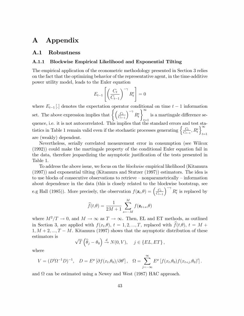
A Appendix

A.1 Robustness

A.1.1 Blockwise Empirical Likelihood and Exponential Tilting

The empirical application of the econometric methodology presented in Section 3 relieson the fact that the optimizing behavior of the representative agent, in the time-additivepower utility model, leads to the Euler equation

Et�1

"�CtCt�1

�� Ret

#= 0

where Et�1 [:] denotes the expectation operator conditional on time t � 1 information

set. The above expression implies that��

CtCt�1

�� Ret

�1t=1

is a martingale di¤erence se-

quence, i.e. it is not autocorrelated. This implies that the standard errors and test sta-

tistics in Table 1 remain valid even if the stochastic processes generatingn

CtCt�1

; Ret

o1t=1

are (weakly) dependent.Nevertheless, serially correlated measurement error in consumption (see Wilcox

(1992)) could make the martingale property of the conditional Euler equation fail inthe data, therefore jeopardizing the asymptotic justi�cation of the tests presented inTable 1.To address the above issue, we focus on the blockwise empirical likelihood (Kitamura

(1997)) and exponential tilting (Kitamura and Stutzer (1997)) estimators. The idea isto use blocks of consecutive observations to retrieve �nonparametrically �informationabout dependence in the data (this is closely related to the blockwise bootstrap, see

e.g Hall (1985)). More precisely, the observation f(zt;�) =�

CtCt�1

�� Ret is replaced by

bf(t;�) = 1

2M + 1

MXs=�M

f(zt+s;�)

where M2=T ! 0, and M ! 1 as T ! 1. Then, EL and ET methods, as outlinedin Section 3, are applied with f(xt;�), t = 1; 2; :::; T , replaced with bf(t;�), t = M +1;M + 2; :::; T �M . Kitamura (1997) shows that the asymptotic distribution of theseestimators is p

T�b�j � �0� d! N(0; V ), j 2 fEL;ETg ;

where

V = (D0�1D)�1, D = E� [@f(xt;�0)=@�0] , =

1Xj=�1

E� [f(xt;�0)f(xt+j;�0)0] :

and can be estimated using a Newey and West (1987) HAC approach.

43

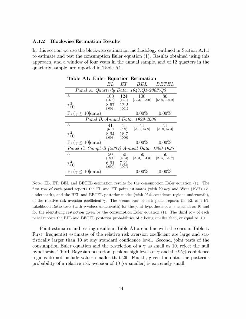
A.1.2 Blockwise Estimation Results

In this section we use the blockwise estimation methodology outlined in Section A.1.1to estimate and test the consumption Euler equation (1). Results obtained using thisapproach, and a window of four years in the annual sample, and of 12 quarters in thequarterly sample, are reported in Table A1.

Table A1: Euler Equation EstimationEL ET BEL BETEL

Panel A. Quarterly Data: 1947:Q1-2003:Q3 100

(16:3)124(12:1)

100[72:3; 133:0]

86[65:0; 107:2]

�2(1) 8:67(:003)

12:2(:001)

Pr ( � 10jdata) 0:00% 0:00%Panel B. Annual Data: 1929-2006

41(5:9)

41(5:9)

41[29:1; 57:9]

41[29:8; 57:4]

�2(1) 8:94(:003)

18:7(:000)

Pr ( � 10jdata) 0:00% 0:00%Panel C. Campbell (2003) Annual Data: 1890-1995 50

(18:4)50(18:4)

50[29:3; 134:3]

50[29:5, 122:7]

�2(1) 6:91(:009)

7:21(:007)

Pr ( � 10jdata) 0:00% 0:00%

Note: EL, ET, BEL and BETEL estimation results for the consumption Euler equation (1). The

�rst row of each panel reports the EL and ET point estimates (with Newey and West (1987) s.e.

underneath), and the BEL and BETEL posterior modes (with 95% con�dence regions underneath),

of the relative risk aversion coe¢ cient . The second row of each panel reports the EL and ET

Likelihood Ratio tests (with p-values underneath) for the joint hypothesis of a as small as 10 and

for the identifying restriction given by the consumption Euler equation (1). The third row of each

panel reports the BEL and BETEL posterior probabilities of being smaller than, or equal to, 10.

Point estimates and testing results in Table A1 are in line with the ones in Table 1.First, frequentist estimates of the relative risk aversion coe¢ cient are large and sta-tistically larger than 10 at any standard con�dence level. Second, joint tests of theconsumption Euler equation and the restriction of a as small as 10, reject the nullhypothesis. Third, Bayesian posteriors peak at high levels of and the 95% con�denceregions do not include values smaller that 29. Fourth, given the data, the posteriorprobability of a relative risk aversion of 10 (or smaller) is extremely small.

44

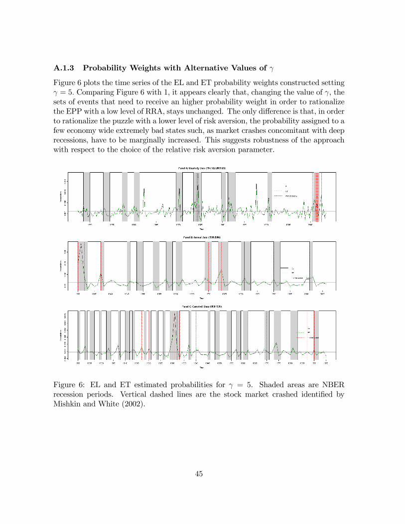
A.1.3 Probability Weights with Alternative Values of

Figure 6 plots the time series of the EL and ET probability weights constructed setting = 5: Comparing Figure 6 with 1, it appears clearly that, changing the value of , thesets of events that need to receive an higher probability weight in order to rationalizethe EPP with a low level of RRA, stays unchanged. The only di¤erence is that, in orderto rationalize the puzzle with a lower level of risk aversion, the probability assigned to afew economy wide extremely bad states such, as market crashes concomitant with deeprecessions, have to be marginally increased. This suggests robustness of the approachwith respect to the choice of the relative risk aversion parameter.

Figure 6: EL and ET estimated probabilities for = 5. Shaded areas are NBERrecession periods. Vertical dashed lines are the stock market crashed identi�ed byMishkin and White (2002).

45

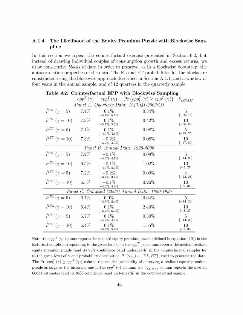
A.1.4 The Likelihood of the Equity Premium Puzzle with Blockwise Sam-pling

In this section we repeat the counterfactual exercise presented in Section 6.2, butinstead of drawing individual couples of consumption growth and excess returns, wedraw consecutive blocks of data in order to preserve, as in a blockwise bootstrap, theautocorrelation properties of the data. The EL and ET probabilities for the blocks areconstructed using the blockwise approach described in Section A.1.1, and a window offour years in the annual sample, and of 12 quarters in the quarterly sample.

Table A2: Counterfactual EPP with Blockwise SamplingeppT ( ) eppTi ( ) Pr

�eppTi ( ) � eppT ( )

� i;GMM

Panel A. Quarterly Data: 1947:Q1-2003:Q3PEL ( = 5) 7:4% 0:1%

[�5:7%, 5:5%]0:34% 5

[�56, 76]

PEL ( = 10) 7:3% 0:1%[�5:7%, 5:5%]

0:42% 10[�56, 80]

PET ( = 5) 7:4% 0:1%[�4:9%, 4:6%]

0:08% 5[�49, 75]

PET ( = 10) 7:3% �0:2%[�5:2%, 4:3%]

0:08% 10[�47, 80]

Panel B. Annual Data: 1929-2006PEL ( = 5) 7:2% �0:1%

[�4:6%, 4:7%]0:08% 5

[�14, 20]

PEL ( = 10) 6:5% �0:1%[�4:9%, 5:4%]

1:02% 10[�5, 27]

PET ( = 5) 7:2% �0:2%[�3:7%, 3:7%]

0:00% 4[�22, 28]

PET ( = 10) 6:5% �0:1%[�4:3%, 4:6%]

0:26% 10[�9, 35]

Panel C. Campbell (2003) Annual Data: 1890-1995PEL ( = 5) 6:7% 0:0%

[�5:5%, 5:4%]0:64% 5

[�14, 29]

PEL ( = 10) 6:4% 0:1%[�6:2%, 6:3%]

2:40% 10[�8, 37]

PET ( = 5) 6:7% 0:1%[�4:7%, 4:5%]

0:30% 5[�14, 29]

PET ( = 10) 6:4% 0:1%[�5:4%, 5:6%]

1:55% 10[�7, 35]

Note: the eppT ( ) column reports the realized equity premium puzzle (de�ned in equation (19)) in the

historical sample corresponding to the given level of ; the eppTi ( ) column reports the median realized

equity premium puzzle (and its 95% con�dence band underneath) in the counterfactual samples for

to the given level of and probability distribution P j ( ), j 2 fEL;ETg, used to generate the data.The Pr

�eppTi ( ) � eppT ( )

�column reports the probability of observing a realized equity premium

puzzle as large as the historical one in the eppT ( ) column; the i;GMM column reports the median

GMM estimates (and its 95% con�dence band underneath) in the counterfactual sample.

46

Results obtained using this approach are reported in Table A2, and the �ndings arelargely in line with the ones in Table 2: the median realized equity premium puzzlein the counterfactual samples is very close to zero and its 95% con�dence region doesnot include the historically observed value; the estimated coe¢ cient of risk aversion inthe counterfactual samples does not have any systematic bias but its 95% con�denceinterval is very large, suggesting that in the presence of rare events this parametermight be dramatically misestimated. Moreover, the probability of observing an equitypremium puzzle in the counterfactual samples is very small, and never larger than2:4%. That is, as Table 2, Table A2 suggests that if one believes that the rare eventshypothesis is the explanation of the EPP, one should also believe that the historicallyobserved EPP is itself a rare event.

A.2 Probability Weighted Fama-MacBeth Regressions

In order to estimate the parameters � and � in equations (22) and (23) we followa Fama and MacBeth (1973) two step procedure, adapted to take into account thatthe moments should be constructed under P j ( ) probability measures instead that assample analogs.In a �rst step, we construct the consumption risk measure in equation (22) by

computing

�j

i : = �CovP

j( )

��CtCt�1

�� ; Rei;t

�EP j( )

��CtCt�1

�� �

= �

PTt=1

�CtCt�1

�� Rei;tp

jt �

�PTt=1

�CtCt�1

�� pjt

� hPTt=1R

ei;tp

jt

i�PT

t=1

�CtCt�1

�� pjt

� ,

where j 2 fEL;ETg, and is �xed to the same value used to construct the weights�pjtTt=1. Similarly, for equation (22) we construct

�j

i : = CovPj( )

�ln

CtCt�1

; Rei;t

�=

TXt=1

ln

�CtCt�1

�Rei;tp

jt �

"TXt=1

ln

�CtCt�1

�pjt

#"TXt=1

Rei;tpjt

#:

In a second step, for each t we run the cross�sectional regression

Rei;t = �t + �j

i�t + "i;t, (26)

47

where "i;t is a mean zero cross-sectional error term, obtaining the sequence of estimatesn�t; �t

oTt=1. The point estimates for � and � are then constructed as

� :=TXt=1

�tpjt and � :=

TXt=1

�tpjt :

Finally, we use the weighted sampling variation ofn�t; �t

oTt=1

to construct the

standard deviations of the above estimators:

�2 (�) :=1

T

TXt=1

(�t � �)2 pjt , �2���:=

1

T

TXt=1

��t � �

�2pjt .

Note that the estimated � and � are numerically equivalent to the coe¢ cients we wouldobtain by running the cross-sectional regression"

TXt=1

Rei;tpjt

#= �+ �

j

i�+ �i

where �i is a mean zero error term.The cross-sectionalR2 corresponding to these Fama andMacBeth (1973) regressions

is constructed as

R2 := 1�V ar

�EP

j( )�Rei;t�� Rei;t

�V ar

�EP j( )

�Rei;t��

where

EPj( )�Rei;t�:=

TXt=1

Rei;tpjt

andRei;t := �+ �

j

i �. (27)

Note that the standard Fama and MacBeth (1973) cross-sectional regression ap-proach (that does not use probability weights) can be recovered by setting pjt = 1=T8t.The estimation algorithm just outlined is the one used to produce the results in

Table 3 of Section 6.3.

48