Chapter 15

Variable-Speed Pumping

MAYO GOTTLIEBSONROBERT L. SANKSALAN VAUSE

CONTRIBUTORSStefan M. AbelinRobert S. BenfellHarrison C. BicknellBruce DensmoreRonald W. DuncanStanley S. HongCasey JonesPaul C. LeachTimothy NanceMichael R. OlsonE. O. PotthoffDouglas L. SchneiderArnold R. SdanoRichard N. SkeehanEarle C. SmithPatricia A. Trager

In this chapter, the uses of variable-speed (V/S) pump

operation in water and wastewater pumping stations

are presented and discussed. The principal adjustable-

and variable-speed drives are reviewed and compared.

The primary goal of V/S wastewater pumping is to

keep the station discharge rate equal to the influent

rate at all times. The station acts as though it were a

sewer discharging by gravity. A pumping station that

meets this goal requires very little storage in the wet

well, does not rapidly cycle any of the pumps, and does

not cause abrupt, large changes in the discharge rate.

The primary goal of V/S booster pumping is to

maintain a nearly constant pressure at all times, re-

gardless of the flow rate. The discussion given here

for V/S booster pumping also applies to high-service

(high-head) pumping for reducing water hammer in

very long transmission mains. Otherwise, V/S is

rarely used for water pumping.

In common usage, the term ‘‘variable speed’’ indi-

cates that the speed of the pump is regulated to pro-

duce the desired flow rate. The term ‘‘variable’’ infers a

change that may or may not be under the control of

the user. ‘‘Adjustable’’ infers a change under the con-

trol of the user. An example of an adjustable-speed

drive is an adjustable-frequency drive (AFD), some-

times mistakenly called a ‘‘variable-frequency’’ drive.

An example of a variable-speed drive is a rheostat-

controlled wound-rotor motor in which, although

speed varies with both load and control, the proper

speed can be attained by the external control.

15.1

‘‘Frequency’’ should only be applied to drives with an

ac output, while the term ‘‘speed’’ is preferred since it

applies to both ac and dc drives as well as to mechan-

ical drive systems. Thus, pump speed can be varied at

will by either an adjustable- or a variable-speed drive.

In this chapter, both kinds of drives are called ‘‘vari-

able-speed’’ or ‘‘V/S’’ for convenience, but when com-

municating with electrical engineers, confusion can be

avoided by strict usage of correct terminology.

Applications to both water and wastewater pump-

ing are described in Sections 15-1, 15-3, and 15-11.

Sections 15-2 and 15-4 through 15-6 are generally

devoted to wastewater pumping, and Sections 15-7

through 15-10 are confined to water booster pumping.

15-1. Variable Speed versus Constant Speed

The difference between V/S and constant-speed (C/S)

pumping is profound and has far-reaching conse-

quences, so the choice should not be lightly made.

Some reasons for the choice of V/S or C/S for a

particular pumping station may be compelling while

others, which may be significant for a different situ-

ation, may be trivial. Nevertheless, all of the reasons

should be considered thoughtfully.

Advantages of Variable-Speed Pumping

The major advantages of V/S pumping, stemming

from the objective that discharge always equals influ-

ent flow rate, are:

. Downstream flow rates fluctuate gradually and do

not upset treatment processes caused by surges, nor

do the sudden surges caused by C/S pumping

pound downstream piping.

. No storage is required, so the wet well can be

smaller, shallower, and less expensive than for

C/S pumping, and size might compensate for the

high cost of the V/S equipment.

. Fewer—although larger—pumps are needed in

medium- to large-sized stations with savings in

space for the pump room and less equipment to

maintain.

. The almost constant wet well surface and short

residence time tend to reduce the production of

odors and corrosive gases.

. Energy savings are likely due to the higher average

wet well surface elevation and the usually lower

pumping rates and lower pipe friction losses.

. Motor life is prolonged because of the infrequent

starts.

. The high inrush current that characterizes across-

the-line starts of C/S drivers is greatly reduced in

V/S drives such as adjustable-frequency drives

(AFDs) and slip-recovery systems (although not in

eddy-current couplings). These reduced inrush cur-

rent starts are referred to as ‘‘soft’’ starts.

. Voltage dips caused by across-the-line starts for

C/S pumps can be substantially reduced with soft

start equipment such as reduced-voltage starters.

Solid-state, reduced-voltage starters are the most

flexible, economical, and space-efficient. They are

usually switched out of the circuit when operating

speed is attained so that harmonic disturbances no

longer occur.

. Throttling the engine of a direct engine drive is a

simple, inexpensive, and reliable means of achiev-

ing V/S, but read Sections 14-2 and 14-22 and

consult the engine manufacturers regarding the

problems of operating diesel or gas engines at less

than full load.

Wastewater

The reasons for using V/S pumping for wastewater

include the following:

. Continuous pumping and the very short liquid

residence time in V/S operation reduces (1) the

deposition of organic solids—a problem in C/S

pumping because of the difficulty of re-suspension;

(2) putrefaction—so the wastewater is easier and

less costly to treat; (3) the production of odors and

corrosive, poisonous gases; and (4) cyclic rise and

fall of the water surface with the resulting pumping

of sewer gases into the atmosphere.

. V/S pumping eliminates the long free fall of waste-

water and the entrainment of air bubbles that, if

sucked into the pump, greatly reduce pump effi-

ciency. However, this advantage disappears in a

comparison with C/S pumping if a sloping ap-

proach pipe is used (see Section 12-7).

. The average static head in C/S pumping can be

reduced by 0.6 m (2 ft) or more in V/S pumping

by keeping the wet well level the same as the nor-

mal level in the influent sewer (see Section 12-6 and

Figure 12-22). Turbulence is thereby virtually elim-

inated and the release of odorous gases is substan-

tially reduced. The energy cost savings due to the

consistently high wet well level may be significant.

. One important reason for using V/S pumping is to

produce gradual changes in flow that do not upset

(and thereby reduce the efficiency of) downstream

processes such as sedimentation. Sudden flow

changes caused by C/S pumps, even at significant

15.2 Chapter 15 Variable-Speed Pumping

distances from a treatment plant, can upset the

entire treatment process. At one utility, it was

found that such flow changes propagated through

the entire primary/secondary treatment process

and were upsetting the dechlorination system. For-

cing the operators to use the V/S drives (which had

been installed but, due to indifference, were not

used) solved the problem.

Water

Water is customarily pumped for long periods (of

several hours) at uniform rates (often to fill reservoirs

or tanks), so—although they may be just as compel-

ling—there are fewer reasons for choosing V/S for

pumping water than for pumping wastewater.

. For booster pumping or pumping into a distribu-

tion system without a reservoir, V/S can provide

constant water pressure during varying rates of

usage. That is the most common application.

. Pumps can be ramped up (or down) slowly so that

water hammer is reduced. (Solid-state starters con-

trolling C/S pumps can also perform this function

if the pipeline is not too long.) In pipelines so long

that 5to is more than 5 min (about 30 km or

20 mi), surges caused by the startup of C/S pumps

can be serious. Solid-state starters or automatically

operated control valves can also reduce water ham-

mer, but only in shorter pipelines. The full-speed

operation of C/S pumps for long periods (more

than several minutes) at near shut-off head causes

excessive wear on pump bearings and flexing of the

shaft.

Disadvantages of Variable-Speed Pumping

The selection of V/S pumping units should only be

made after due consideration of the disadvantages.

. Except for engine drives, V/S adds significant cost

and complexity, requires more equipment and

more maintenance, and reduces reliability.

Troubleshooting and repairs require personnel

with on-the-job training. Each type of V/S drive

requires a different kind of specialized training.

. If the operating personnel do not understand the

equipment or find it difficult to maintain, they are

likely to turn off the V/S drive, operate the pumps

manually at C/S, and thus effectively lose the

investment in expensive equipment plus the advan-

tages it offers. Pump sumps designed for V/S

pumping have insufficient storage for C/S pump-

ing, and the frequent starting may burn out the

motors and certainly reduces their life.

. V/S drives have less electrical efficiency than C/S

motor drives (although V/S drives may use less

energy because of lower pipeline friction losses).

. Avoiding vibration is more difficult with variable

drive shaft speeds because the ‘‘windows’’ (the

ranges of allowable supporting structure frequen-

cies) for avoiding resonance are narrower. This

avoidance should always be by design—never by

luck (see Chapter 22).

. Instrumentation for regulating pump speed must

usually be more refined, accurate, and costly than

is required for C/S pumping.

. V/S drives are not well adapted to flat system H-Q

curves because (1) good efficiencies cannot be

obtained throughout the speed range; (2) small

changes in speed produce large changes in dis-

charge; and (3) energy losses (and costs) are high.

. Rapid changes in technology can make particular

models obsolete.

. V/S drives may be much noisier than C/S drives.

. AFDs, in particular, are more vulnerable to light-

ning and electrical disturbances.

The disadvantages of V/S pumping are essentially

advantages for C/S pumping. To complete the com-

parison, consider the following:

. The cost of the large wet wells required for C/S

pumping may exceed the cost of V/S drives, but

note that excavation costs are site-dependent.

. Pump sizes and wet well design can be easily

coordinated so that the number of pump starts

per hour (for C/S pumps) is well within acceptable

limits.

. A wide range of flow rates can also be accommo-

dated by using several C/S pumps, and the pro-

grammers for alternating C/S pumps are more

reliable and less expensive than control systems

for V/S units. A penalty for using C/S pumps is a

larger station, more pumping units, more piping

and fittings, and discrete increments of flow.

. Surges due to starting or stopping one pump are

not as severe as those caused by a power failure,

which may occur when several pumps are running

and for which the station and pipeline must be

protected from water hammer anyway. Solid-state

starters or pump-control valves can eliminate

surges in usual circumstances. If the pumping sta-

tion discharges a small proportion of the treatment

plant flow, the sudden change of influent flow rate

due to the starting and stopping of a single pump

may be negligible. The effect cannot be quantified,

so this is a matter of judgment.

15-1. Variable Speed versus Constant Speed 15.3

. Relatively constant water pressure from a booster

pumping station may be obtained with C/S pumps

either with flat H-Q curves (if suction pressure is

constant) or with elevated or pressurized tanks.

Summary

If objective evaluation of these advantages and dis-

advantages leads to a decision to use V/S, select the

best drive for the particular application.

15-2. Design Considerations

Firm pumping capacity is the maximum station dis-

charge with the largest pump out of service. Similarly,

a station with V/S pumps must be able to accommo-

date any flow (from minimum to maximum) and

operate in a normal manner when any one of the

pumps or drives is out of service.

A V/S pumping station that includes C/S pumps

can provide the same results as a station with all V/S

pumps, but only if the relationship between the sizes

of the two kinds of pumps is correct (see Sections 15-5

and 15-10).

Pumps

The number of pumps to be installed in a station

depends on (1) the range over which the influent

flow rate varies, (2) the available pump selections,

(3) the optimization of size of wet well versus the

size of pumps, and (4) operating costs.

Wet Wells

For V/S pumping, the wet well need only be a sump

for pumping at the instantaneous system flow rate.

The only storage required is enough to allow pumps

to be shut down or started up without an excessive

change in water level, and the water surface area

needed for that purpose is quite small.

Furthermore, the change of water surface elevation

can be reduced to the amount needed for regulating the

speedof thepumps.MostV/S control systems start and

stop the pumps and regulate speed over a range of

about 0.6 m (2 ft) of change in the water elevations in

the wet well. (An even smaller range can be used, but a

more sophisticated control system may be required.)

Hence, some static head canbe saved as comparedwith

a C/S pumping system in which the wet well level

typically fluctuates over a range of 1.2 m (4 ft)

or more. Detailed designs of wet wells for V/S and C/

S pumping are given in Examples 12-1 and 12-2.

15-3. Theory of Variable-Speed Pumping

It may be helpful to review the fundamental theory

for centrifugal pumps in Section 10-3, which was

explained primarily by Equations 10-15 through

10-21 and by Examples 10-2, 10-3, and 10-8.

In pump manufacturers’ published data, H-Q

curves are usually shown for impellers of several

diameters at two or more speeds. Such curves drawn

for pump speeds of 880, 695, and 585 rev/min are

shown in Figure 15-1. At variable speeds, the pump

actually operates on an infinite number of speed

curves between the maximum and minimum limits.

The minimum speed may be less than the lowest

speed for which a published curve is available.

Most nonclog, dry-well wastewater pumps can be

furnished with an impeller of any diameter desired

between the minimum and maximum shown. For

example, if the pump whose curves are shown in

Figure 15-1 must deliver a maximum of 0:35 m3=sat 15.2 m (5500 gal/min at 50 ft), the curve for that

impeller would pass through those coordinates and

would be represented by the dashed lined labeled

20.1 in. (impeller diameter).

Speed versus Flow Curves

When discharging into a hydraulic system, the pump

must operate on the system head-capacity (H-Q)

curve at all flows. In Figure 15-2, a typical system

H-Q curve has been superimposed on the 20.1-in.

diameter impeller curves. The pump delivers

0:133m3=s (2100 gal/min) at 10.8 m (35.5 ft) when it

operates at 585 rev/min; 0:227m3=s (3600 gal/min) at

12.3 m (40.5 ft) at 695 rev/min; and 0:347m3=s(5500 gal/min) at 15.2 m (50 ft) at 880 rev/min.

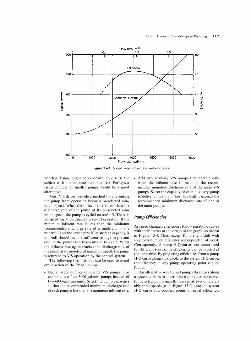
A curve of speed versus flow rate can be plotted

from these data, as in Figure 15-3. This curve is

probably the most meaningful depiction of V/S

pump operation for a single pump. Note that the

pump efficiencies (obtained from Figure 15-1) vary

from 70% at maximum flow rate through 83% at

midspeed to 77% at low speed—good efficiencies

throughout the usual flow rate rates.

Affinity Law for Speed

To determine a speed versus flow curve for any pump

impeller, find the flow rates at which three or more of

15.4 Chapter 15 Variable-Speed Pumping

the pump H-Q curves (each at a different speed) inter-

sect the system H-Q curve. If only one or two of the

published pump curves intersects the system curve,

points on another speed curve can be calculated from

the affinity laws as shown in Example 10-2, Section

10-3. Note, incidentally, that points along the system

Figure 15-1. Pump characteristic curves at three speeds.

15-3. Theory of Variable-Speed Pumping 15.5

H-Q curve are not ‘‘corresponding points’’ and, hence,

the flow rate is not proportional to pump speed.

Minimum Operating Speed

The minimum operating pump shaft speed (zero Q

speed) is defined as the speed at which the pump is no

longer able to maintain discharge against the static

head. Hence, it is unique for each pump and each

pumping station, and it occurs at the speed for which

the pump’s shut-off head equals the static head.

At zero discharge (zero Q), and only at zero Q, the

pump discharge head can change without a change in

the flow rate. Hence, at this unique locus of points,

Equation 10-16 is the only one needed for calculating

the zero Q speed for a pump discharging into a

hydraulic system. Solving that equation for the

pump and system H-Q curve in Figure 15-2 gives

n1 ¼ n2

ffiffiffiffiffiffiH1

H2

r¼ 585

ffiffiffiffiffi33

45

r¼ 501 rev=min (15-1)

and a position of the curve for this speed is shown as

a dashed line in Figure 15-2. However, most pumps,

especially medium and large ones, should not be

operated more than momentarily at zero flow. At

zero flow and at low discharge rates, the pumped

fluid recirculates within the volute, which causes an

unbalanced radial thrust against the impeller that

results in a flexing of the pump shaft, which can

cause bearing failure or fatigue fracture of the shaft

(see Section 10-6).

As a rule of thumb, it is usually safe to operate a

pump continuously at discharge rates of 30% or more

of its best efficiency capacity (BEC), which is its

discharge capacity at the best efficiency point (BEP)

at the maximum recommended speed. The pump

manufacturer’s minimum discharge rate, however,

should always be met; the minimum recommendation

may be 50% or more of BEC for some pumps. By

requiring custom-engineered pumps (heavier shafts

and bearings), the problem with the minimum recom-

mended operating speed can be avoided with most

pump makes. But a custom pump, especially in a

Figure 15-2. Pump characteristic curves for a 20.1-in. impeller.

15.6 Chapter 15 Variable-Speed Pumping

nonclog design, might be expensive, so discuss the

subject with one or more manufacturers. Perhaps a

larger number of smaller pumps would be a good

alternative.

Most V/S drives provide a method for preventing

the pump from operating below a preselected min-

imum speed. When the influent rate is less than the

discharge rate of the pump at its preselected min-

imum speed, the pump is cycled on and off. There is

no speed variation during the on-off operation. If the

minimum influent rate is less than the minimum

recommended discharge rate of a single pump, the

wet well (and the sewer pipe if its storage capacity is

utilized) should include sufficient storage to prevent

cycling the pumps too frequently at this rate. When

the influent rate again reaches the discharge rate of

the pump at its preselected minimum speed, the pump

is returned to V/S operation by the control system.

The following two methods can be used to avoid

cyclic action of the ‘‘lead’’ pump:

. Use a larger number of smaller V/S pumps. For

example, use four 3000-gal/min pumps instead of

two 6000-gal/min units. Select the pump capacities

so that the recommended minimum discharge rate

of each pump is less than theminimum influent rate.

. Add two auxiliary V/S pumps that operate only

when the influent rate is less than the recom-

mended minimum discharge rate of the main V/S

pumps. Select the capacity of each auxiliary pump

to deliver a maximum flow that slightly exceeds the

recommended minimum discharge rate of one of

the main pumps.

Pump Efficiencies

As speed changes, efficiencies follow parabolic curves

with their apexes at the origin of the graph, as shown

in Figure 15-4. Thus, except for a slight shift with

Reynolds number, efficiency is independent of speed.

Consequently, if pump H-Q curves are constructed

for different speeds, the efficiencies can be plotted at

the same time. By projecting efficiencies from a pump

H-Q curve along a parabola to the system H-Q curve,

the efficiency at any pump operating point can be

found.

An alternative way to find pump efficiencies along

a system curve is to superimpose characteristic curves

for selected pump impeller curves at two or prefer-

ably three speeds (as in Figure 15-2) onto the system

H-Q curve and connect points of equal efficiency.

Figure 15-3. Speed versus flow rate and efficiency.

15-3. Theory of Variable-Speed Pumping 15.7

The pump efficiencies along the system H-Q curve

can then be plotted as shown in Figure 15-4.

Power Required

When the pump discharges into a hydraulic system,

the power delivered by the pump at any point on the

system head curve is determined by the flow rate and

the head at that point (see Equation 10-6).

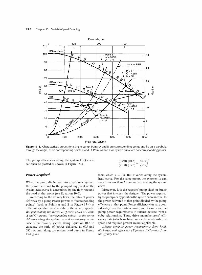
According to the affinity laws, the ratio of power

delivered by a pump (water power) at ‘‘corresponding

points’’ (such as Points A and B in Figure 15-4) at

different speeds equals the cube of the ratio of speeds.

But points along the system H-Q curve (such as Points

A and C) are not ‘‘corresponding points,’’ so the power

delivered along the system curve does not vary as the

cube of the ratio of speeds. Using Equation 10-6 to

calculate the ratio of power delivered at 695 and

585 rev/ min along the system head curve in Figure

15-4 gives:

(3550) (40:5)

(2100) (35:5)¼ 695

585

� �x

from which x ¼ 3.8. But x varies along the system

head curve. For the same pump, the exponent x can

vary from less than 2 to more than 4 along the system

curve.

Moreover, it is the required pump shaft or brake

power that interests the designer. The power required

by thepumpatanypoint on the systemcurve is equal to

the power delivered at that point divided by the pump

efficiency at that point. Pump efficiency can vary con-

siderably over the system curve, and it can cause the

pump power requirements to further deviate from a

cube relationship. Thus, drive manufacturers’ effi-

ciency data (which are based on a cube relationship of

speed and required power) are not applicable.

Always compute power requirements from head,

discharge, and efficiency (Equation 10-7)—not from

the affinity laws.

Figure 15-4. Characteristic curves for a single pump. Points A and B are corresponding points and lie on a parabolathrough the origin, as do corresponding points C and D. Points A and C on system curve are not corresponding points.

15.8 Chapter 15 Variable-Speed Pumping

15-4. Pump Selection

All of the arrangements described here include suffi-

cient pumping capacity to discharge the peak influent

rate when any single pump is out of service.

Two-Pump Facility

For an installation with two pumps, each capable of

discharging the peak influent rate, a single duty pump

with its peak discharge rate well to the right of the

BEP provides satisfactory efficiencies throughout the

entire operating range, and very good efficiencies in

the center of the range. An example of the capability

of a single pump is shown in Figure 15-4. Note that

the efficiencies are 69% or more over a range of flows

equal to 2.75:1.

Three Variable-Speed Pumps

In the usual arrangement of a three-V/S-pump sys-

tem, two pumps must be capable of discharging the

design flow rate, while the third is idle as a standby

unit. Unless the system curve is flat, a single pump

must be capable of discharging somewhat more than

one-half of the peak influent rate. The ‘‘lead’’ pump

runs alone during periods of low flow. The ‘‘lag’’

pump is started when the influent rate slightly exceeds

the maximum discharge rate of the lead pump, and

both pumps operate until the influent rate again falls

to slightly within the capability of the lead unit.

Assume, for example, that a pumping station must

discharge flow rates from 0:13m3=s (2000 gal/min) to

0:50m3=s (8000 gal/min) at a static lift of 10 m (33 ft)

and a TDH at peak discharge of 20 m (67 ft). The

system H-Q curve is shown in Figures 15-4 and 15-5.

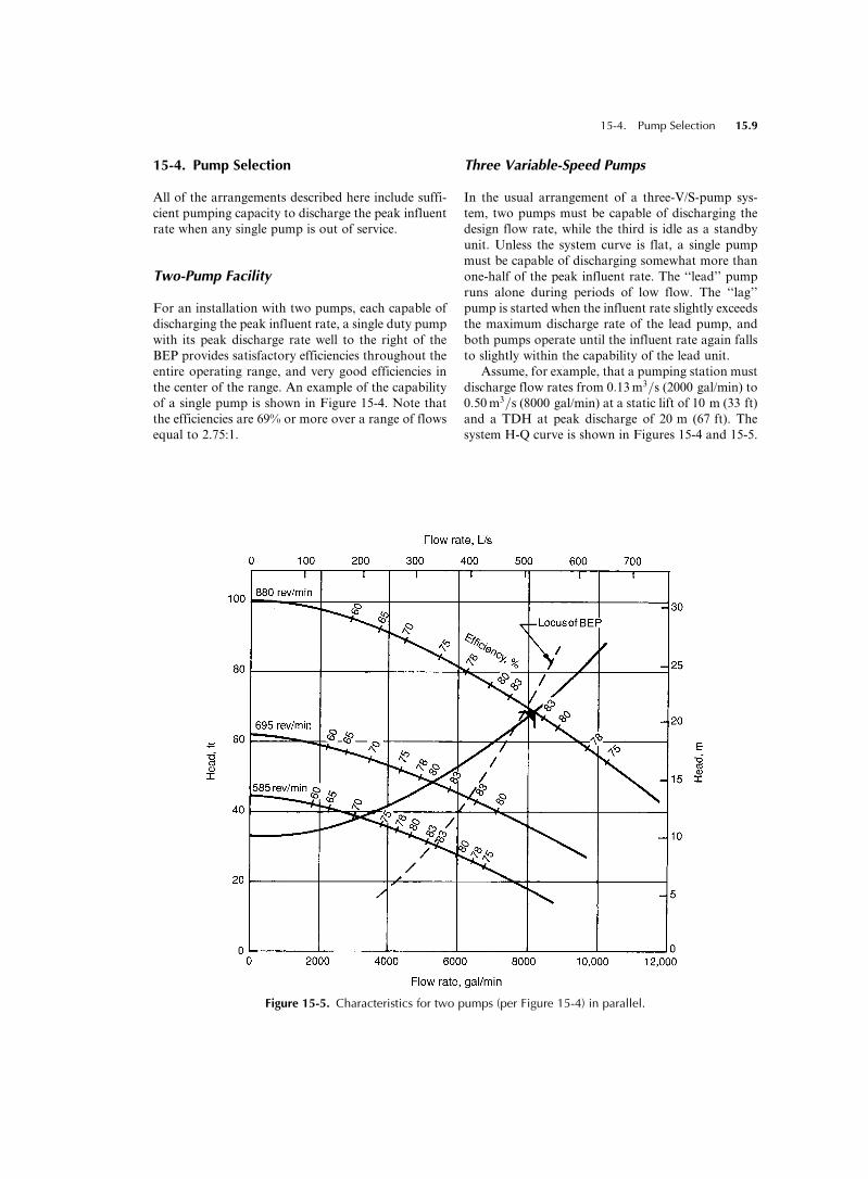
Figure 15-5. Characteristics for two pumps (per Figure 15-4) in parallel.

15-4. Pump Selection 15.9

The friction head is moderate and the curve is rela-

tively flat, so a pump with comparatively steep H-Q

curves should be selected. When two pumps are op-

erating, the BEP should be to the left of the operating

point at peak flow rate so that the system H-Q curve

sweeps across the curves of highest efficiency. There-

fore, the BEP of a single pump at top speed (880 rev/

min in Figure 15-4) should be at the left of the mid-

range discharge [0:35m3=s (5500 gal/min)], and for a

single pump operating, only the higher efficiency

curves should straddle the system H-Q curve. The

minimum discharge should be at least 30% of the

maximum. The pump depicted meets all of these

requirements and thus appears to be a good choice.

Load-Sharing Operation

When two of the above pumps operate in parallel at

the same speed, the discharge (abscissa) is doubled

with no change of head (ordinate), as is shown in

Figure 15-5. (Review Figure 10-24 and the accom-

panying text if an explanation is needed.) Note that

the locus of BEP for the two pumps at full speed is

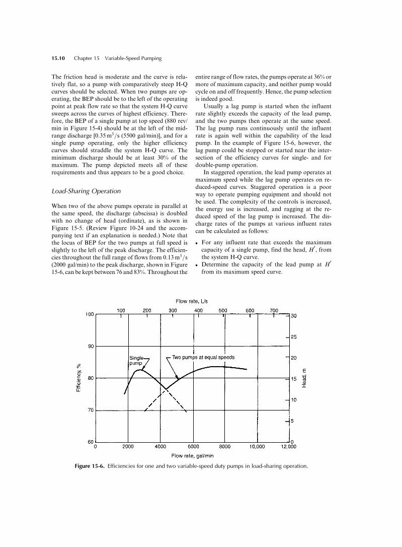
slightly to the left of the peak discharge. The efficien-

cies throughout the full range of flows from 0:13m3=s(2000 gal/min) to the peak discharge, shown in Figure

15-6, can be kept between 76 and 83%. Throughout the

entire range of flow rates, the pumps operate at 36% or

more of maximum capacity, and neither pump would

cycle on and off frequently. Hence, the pump selection

is indeed good.

Usually a lag pump is started when the influent

rate slightly exceeds the capacity of the lead pump,

and the two pumps then operate at the same speed.

The lag pump runs continuously until the influent

rate is again well within the capability of the lead

pump. In the example of Figure 15-6, however, the

lag pump could be stopped or started near the inter-

section of the efficiency curves for single- and for

double-pump operation.

In staggered operation, the lead pump operates at

maximum speed while the lag pump operates on re-

duced-speed curves. Staggered operation is a poor

way to operate pumping equipment and should not

be used. The complexity of the controls is increased,

the energy use is increased, and ragging at the re-

duced speed of the lag pump is increased. The dis-

charge rates of the pumps at various influent rates

can be calculated as follows:

. For any influent rate that exceeds the maximum

capacity of a single pump, find the head, H’, fromthe system H-Q curve.

. Determine the capacity of the lead pump at H’from its maximum speed curve.

Figure 15-6. Efficiencies for one and two variable-speed duty pumps in load-sharing operation.

15.10 Chapter 15 Variable-Speed Pumping

. The discharge rate of the lag pump equals the

influent rate minus the lead pump capacity.

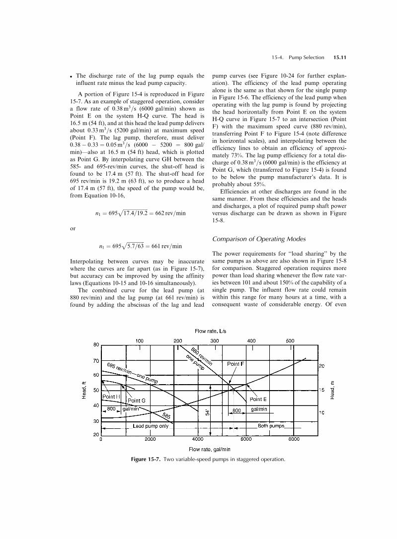
A portion of Figure 15-4 is reproduced in Figure

15-7. As an example of staggered operation, consider

a flow rate of 0:38m3=s (6000 gal/min) shown as

Point E on the system H-Q curve. The head is

16.5 m (54 ft), and at this head the lead pump delivers

about 0:33m3=s (5200 gal/min) at maximum speed

(Point F). The lag pump, therefore, must deliver

0:38� 0:33 ¼ 0:05m3=s (6000 � 5200 ¼ 800 gal/

min)—also at 16.5 m (54 ft) head, which is plotted

as Point G. By interpolating curve GH between the

585- and 695-rev/min curves, the shut-off head is

found to be 17.4 m (57 ft). The shut-off head for

695 rev/min is 19.2 m (63 ft), so to produce a head

of 17.4 m (57 ft), the speed of the pump would be,

from Equation 10-16,

n1 ¼ 695ffiffiffiffiffiffiffiffiffiffiffiffiffiffiffiffiffiffiffiffi17:4=19:2

p¼ 662 rev=min

or

n1 ¼ 695ffiffiffiffiffiffiffiffiffiffiffiffiffiffi5:7=63

p¼ 661 rev=min

Interpolating between curves may be inaccurate

where the curves are far apart (as in Figure 15-7),

but accuracy can be improved by using the affinity

laws (Equations 10-15 and 10-16 simultaneously).

The combined curve for the lead pump (at

880 rev/min) and the lag pump (at 661 rev/min) is

found by adding the abscissas of the lag and lead

pump curves (see Figure 10-24 for further explan-

ation). The efficiency of the lead pump operating

alone is the same as that shown for the single pump

in Figure 15-6. The efficiency of the lead pump when

operating with the lag pump is found by projecting

the head horizontally from Point E on the system

H-Q curve in Figure 15-7 to an intersection (Point

F) with the maximum speed curve (880 rev/min),

transferring Point F to Figure 15-4 (note difference

in horizontal scales), and interpolating between the

efficiency lines to obtain an efficiency of approxi-

mately 73%. The lag pump efficiency for a total dis-

charge of 0:38m3=s (6000 gal/min) is the efficiency at

Point G, which (transferred to Figure 15-4) is found

to be below the pump manufacturer’s data. It is

probably about 55%.

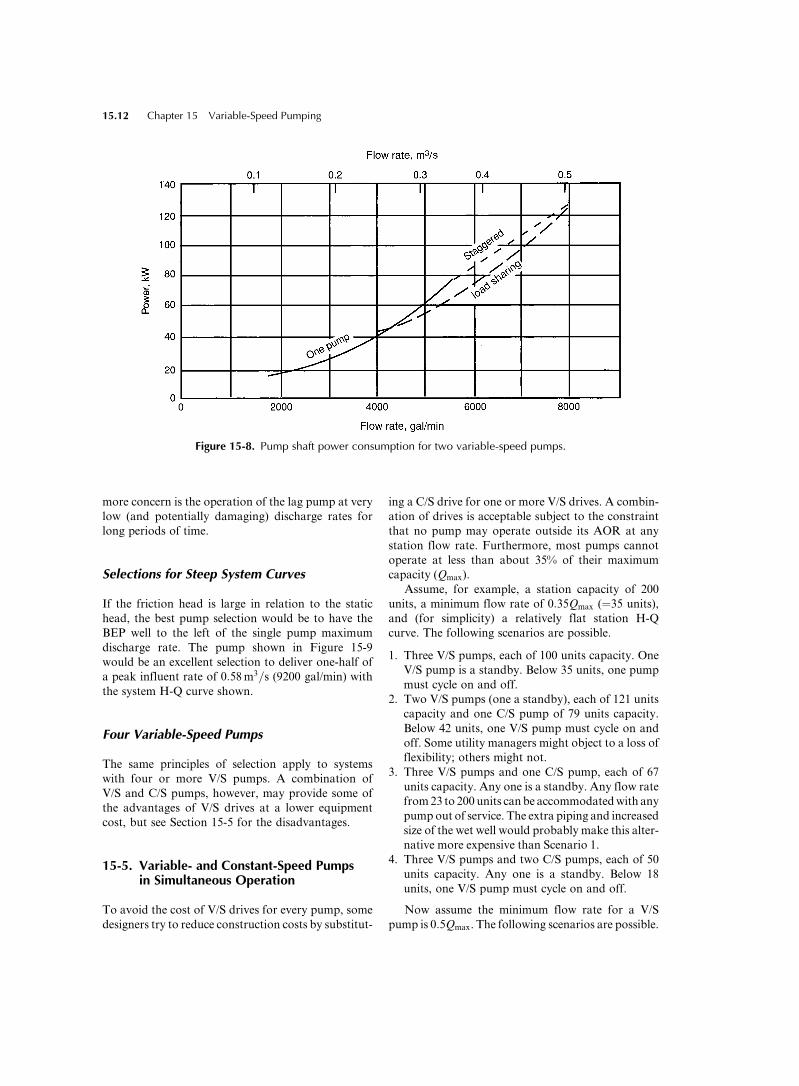
Efficiencies at other discharges are found in the

same manner. From these efficiencies and the heads

and discharges, a plot of required pump shaft power

versus discharge can be drawn as shown in Figure

15-8.

Comparison of Operating Modes

The power requirements for ‘‘load sharing’’ by the

same pumps as above are also shown in Figure 15-8

for comparison. Staggered operation requires more

power than load sharing whenever the flow rate var-

ies between 101 and about 150% of the capability of a

single pump. The influent flow rate could remain

within this range for many hours at a time, with a

consequent waste of considerable energy. Of even

Figure 15-7. Two variable-speed pumps in staggered operation.

15-4. Pump Selection 15.11

more concern is the operation of the lag pump at very

low (and potentially damaging) discharge rates for

long periods of time.

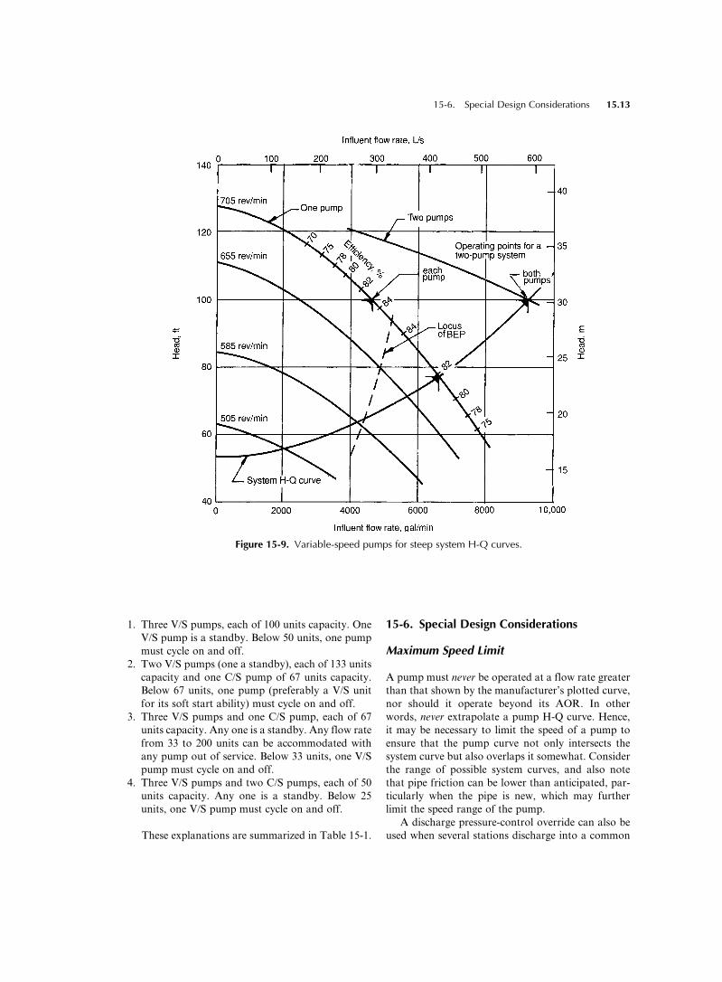
Selections for Steep System Curves

If the friction head is large in relation to the static

head, the best pump selection would be to have the

BEP well to the left of the single pump maximum

discharge rate. The pump shown in Figure 15-9

would be an excellent selection to deliver one-half of

a peak influent rate of 0:58m3=s (9200 gal/min) with

the system H-Q curve shown.

Four Variable-Speed Pumps

The same principles of selection apply to systems

with four or more V/S pumps. A combination of

V/S and C/S pumps, however, may provide some of

the advantages of V/S drives at a lower equipment

cost, but see Section 15-5 for the disadvantages.

15-5. Variable- and Constant-Speed Pumpsin Simultaneous Operation

To avoid the cost of V/S drives for every pump, some

designers try to reduce construction costs by substitut-

ing a C/S drive for one or more V/S drives. A combin-

ation of drives is acceptable subject to the constraint

that no pump may operate outside its AOR at any

station flow rate. Furthermore, most pumps cannot

operate at less than about 35% of their maximum

capacity (Qmax).

Assume, for example, a station capacity of 200

units, a minimum flow rate of 0:35Qmax (¼35 units),

and (for simplicity) a relatively flat station H-Q

curve. The following scenarios are possible.

1. Three V/S pumps, each of 100 units capacity. One

V/S pump is a standby. Below 35 units, one pump

must cycle on and off.

2. Two V/S pumps (one a standby), each of 121 units

capacity and one C/S pump of 79 units capacity.

Below 42 units, one V/S pump must cycle on and

off. Some utility managers might object to a loss of

flexibility; others might not.

3. Three V/S pumps and one C/S pump, each of 67

units capacity. Any one is a standby. Any flow rate

from23 to 200 units canbe accommodatedwith any

pump out of service. The extra piping and increased

size of the wet well would probably make this alter-

native more expensive than Scenario 1.

4. Three V/S pumps and two C/S pumps, each of 50

units capacity. Any one is a standby. Below 18

units, one V/S pump must cycle on and off.

Now assume the minimum flow rate for a V/S

pump is 0:5Qmax. The following scenarios are possible.

Figure 15-8. Pump shaft power consumption for two variable-speed pumps.

15.12 Chapter 15 Variable-Speed Pumping

1. Three V/S pumps, each of 100 units capacity. One

V/S pump is a standby. Below 50 units, one pump

must cycle on and off.

2. Two V/S pumps (one a standby), each of 133 units

capacity and one C/S pump of 67 units capacity.

Below 67 units, one pump (preferably a V/S unit

for its soft start ability) must cycle on and off.

3. Three V/S pumps and one C/S pump, each of 67

units capacity. Any one is a standby. Any flow rate

from 33 to 200 units can be accommodated with

any pump out of service. Below 33 units, one V/S

pump must cycle on and off.

4. Three V/S pumps and two C/S pumps, each of 50

units capacity. Any one is a standby. Below 25

units, one V/S pump must cycle on and off.

These explanations are summarized in Table 15-1.

15-6. Special Design Considerations

Maximum Speed Limit

A pump must never be operated at a flow rate greater

than that shown by the manufacturer’s plotted curve,

nor should it operate beyond its AOR. In other

words, never extrapolate a pump H-Q curve. Hence,

it may be necessary to limit the speed of a pump to

ensure that the pump curve not only intersects the

system curve but also overlaps it somewhat. Consider

the range of possible system curves, and also note

that pipe friction can be lower than anticipated, par-

ticularly when the pipe is new, which may further

limit the speed range of the pump.

A discharge pressure-control override can also be

used when several stations discharge into a common

Figure 15-9. Variable-speed pumps for steep system H-Q curves.

15-6. Special Design Considerations 15.13

force main where the head at any station can be very

low at times.

Control of Pumping Units

A pump-control system should be designed so that the

failure of any component or the trip of any single

protective device (downstream from the main breaker)

does not disable more than one pump. A complete and

separate V/S drive for each V/S pump is strongly

recommended to ensure that the facility can operate

in a normal manner with any single V/S drive out of

service.

Pump Failure Detection

Pump failure detection is a highly desirable feature

that can usually be included in the pump-control

system at little cost. If the pumps are equipped with

outside-lever check valves, the valves can be fitted

with limit (position) switches to detect check valve

arm movement and therefore flow (or the lack of

flow). The limit switch is actuated by the lever when

the valve is fully closed; it is deactivated when the

pump begins to deliver a small flow rate. Regardless

of the cause, the check valve limit switch can detect

the failure of the pump to discharge.

The electrical circuitry is designed to de-energize

the motor of any pump whose check valve remains

closed for a predetermined period of time (usually less

than 3 min for V/S pumps) when the pump is required

to operate. An alarm is signaled, and the standby

pump replaces the unit that failed.

Check valve limit switches can also prevent ener-

gization of the motor of any pumping unit whose

discharge check valve is not fully closed. Some drives

can be severely damaged or destroyed and shafts can

break if the motor is energized while the pump is

back-spinning.

If the check valves do not have outside levers, a

pressure switch located between the pump discharge

nozzle and the check valve is sometimes used as a

flow sensor. Actually, the check valve only indicates

pressure, not flow, and is misleading if flow is

blocked by a downstream obstruction. A better

flow indicator is a vane switch in clean water appli-

cations and, for wastewater, a thermal-dispersion

switch or a Doppler flow switch (see Section 20-5).

When used for wastewater or dirty water, any pres-

sure device (such as a bourdon tube) should be filled

with a clear liquid (glycerin, for example), which is

separated from the dirty water by a flexible dia-

phragm. See Figure 20-6.

Power-Operated Check Valves

If the pump discharge check valves are power-

operated (hydraulic or electric), it may be necessary

to include a relatively sophisticated control system

to protect the V/S pump drives against back-spinning

while the drives are energized. When a pumping

unit is required to operate and the pump drive is

activated, the check valve should not begin to open

until the pressure on the upstream side of the valve

exceeds the pressure on the downstream side. (The

pressure can be sensed, as described previously.)

When the pump is no longer needed, the check

valve should close first, and the pump should

not be stopped until the valve is at least 95%

closed.

Table 15-1. Station Flow Rates for Various Combinations of V/S and C/S Pumps

Scenario V/S pumps C/S pumps Standby Max flow rate Min flow rate

For minimum flow rate in any V/S pump at 35% capacity:

1 3 @ 100 0 1 V/S 200 35

2 2 @ 121 1 @ 79 1 V/S 200 43

3 3 @ 67 1 @ 67 1 C/S or V/S 201 23

4 3 @ 50 2 @ 50 1 C/S or V/S 200 18

For minimum flow rate in a V/S pump at 50% capacity:

1 3 @ 100 0 1 V/S 200 50

2 2 @ 133 1 @ 67 1 V/S 200 67

3 3 @ 67 1 @ 67 1 C/S or V/S 201 33

4 3 @ 50 2 @ 50 1 C/S or V/S 200 25

Note that in Scenarios 2, 3, and probably 4, the C/S pump will operate very little of the time. The total cost of these scenarios (especially

Scenario 4) may be greater than that of Scenario 1.

15.14 Chapter 15 Variable-Speed Pumping

The pumping unit should be de-energized when:

. The pump discharge pressure does not exceed the

pressure in the force main within a short interval

(say, 60 s) after the pump is started.

. The check valve does not open fully within a few

minutes after the pump discharge pressure exceeds

the pressure downstream from the check valve.

. The check valve does not close fully within a short

interval (say, 3 min) after the pumping unit is sig-

naled to shut down.

The control system should also prevent energiza-

tion of the motor of any drive whose check valve is

not fully closed.

15-7. Analysis of Variable-Speed BoosterPumping

The purpose of a V/S booster pump is to maintain a

nearly constant discharge pressure while delivering

the variable flow rate needed in a closed distribution

network. Pump speed variation controls the pump

discharge pressure, and the flow rate is determined

by the system demand.

To analyze the operation of a pump that dis-

charges into a hydraulic network, both the V/S

pump characteristic curves and the curve of required

pump differential head versus flow rate must be con-

sidered. The pump must always operate at the inter-

section of the impeller’s characteristic curve (at the

speed of rotation) with the required differential head

curve.

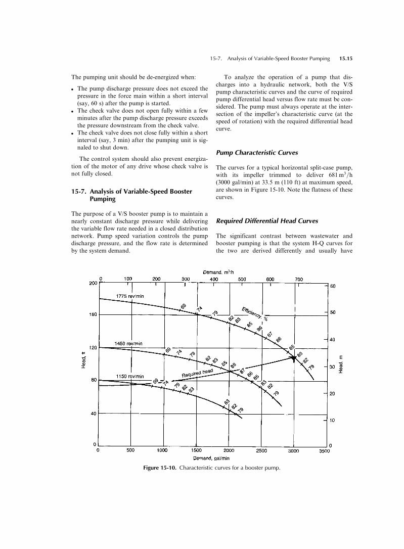
Pump Characteristic Curves

The curves for a typical horizontal split-case pump,

with its impeller trimmed to deliver 681m3=h(3000 gal/min) at 33.5 m (110 ft) at maximum speed,

are shown in Figure 15-10. Note the flatness of these

curves.

Required Differential Head Curves

The significant contrast between wastewater and

booster pumping is that the system H-Q curves for

the two are derived differently and usually have

Figure 15-10. Characteristic curves for a booster pump.

15-7. Analysis of Variable-Speed Booster Pumping 15.15

different shapes. The system H-Q curve for a booster

pumping facility is actually a ‘‘required differential

head,’’ which represents the differential head that

must be added to the suction head to produce the

desired constant discharge pressure at all flow rates.

There are four basic types of suction pressure

variation.

. The suction pressure decreases with an increase of

the pump discharge flow rate due to headlosses in

the suction piping system.

. The suction pressure remains constant regardless

of flow rate. An example is a pump that takes

suction directly from a tank in which the water

level is automatically maintained relatively con-

stant by a float valve on the supply inlet.

. The suction pressure varies independently of flow

rate. An example is a relatively small pump that

takes suction from a large city main in which the

pressure varies but is essentially unaffected by flow

through the pump. Thus, there are an infinite num-

ber of suction head curves.

. The suction pressure decreases with an increase in

the pump discharge rate and also varies independ-

ently of flow rate. Examples are (1) a booster pump

in a city water main in which pressure varies due

both to the pump discharge and to other demands,

and (2) an in-line transmission booster pump.

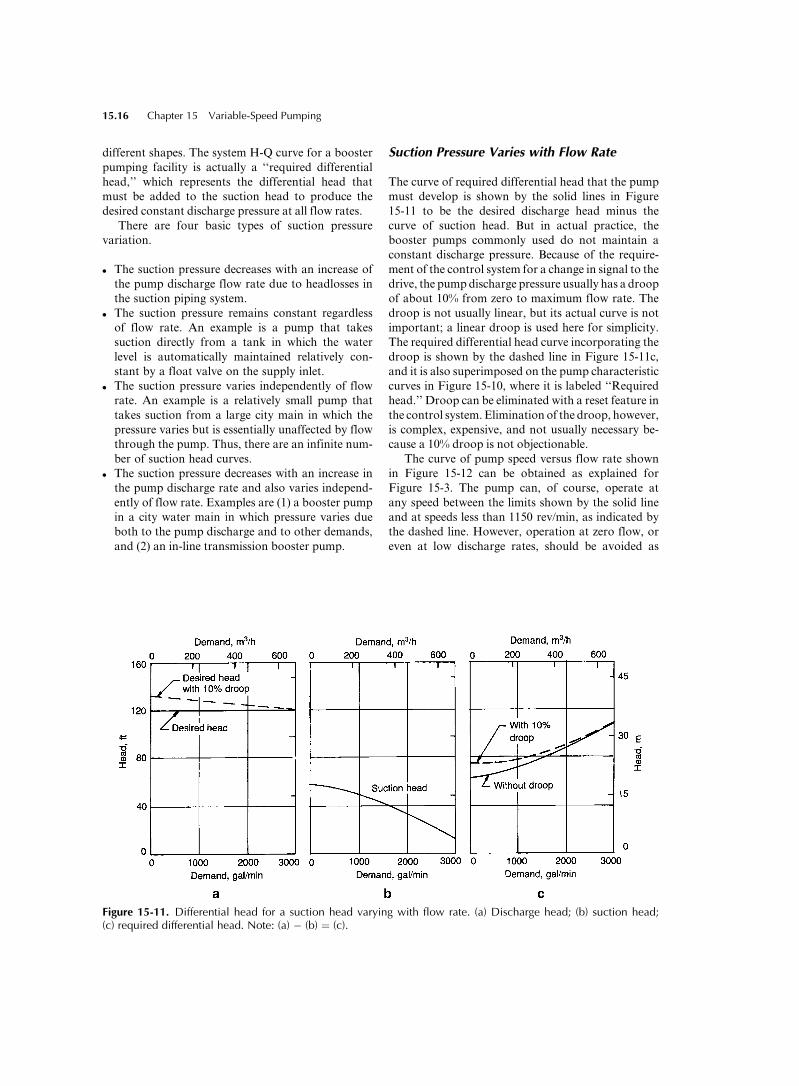
Suction Pressure Varies with Flow Rate

The curve of required differential head that the pump

must develop is shown by the solid lines in Figure

15-11 to be the desired discharge head minus the

curve of suction head. But in actual practice, the

booster pumps commonly used do not maintain a

constant discharge pressure. Because of the require-

ment of the control system for a change in signal to the

drive, the pumpdischarge pressure usually has a droop

of about 10% from zero to maximum flow rate. The

droop is not usually linear, but its actual curve is not

important; a linear droop is used here for simplicity.

The required differential head curve incorporating the

droop is shown by the dashed line in Figure 15-11c,

and it is also superimposed on the pump characteristic

curves in Figure 15-10, where it is labeled ‘‘Required

head.’’ Droop can be eliminated with a reset feature in

the control system.Elimination of the droop, however,

is complex, expensive, and not usually necessary be-

cause a 10% droop is not objectionable.

The curve of pump speed versus flow rate shown

in Figure 15-12 can be obtained as explained for

Figure 15-3. The pump can, of course, operate at

any speed between the limits shown by the solid line

and at speeds less than 1150 rev/min, as indicated by

the dashed line. However, operation at zero flow, or

even at low discharge rates, should be avoided as

Figure 15-11. Differential head for a suction head varying with flow rate. (a) Discharge head; (b) suction head;(c) required differential head. Note: (a) � (b) ¼ (c).

15.16 Chapter 15 Variable-Speed Pumping

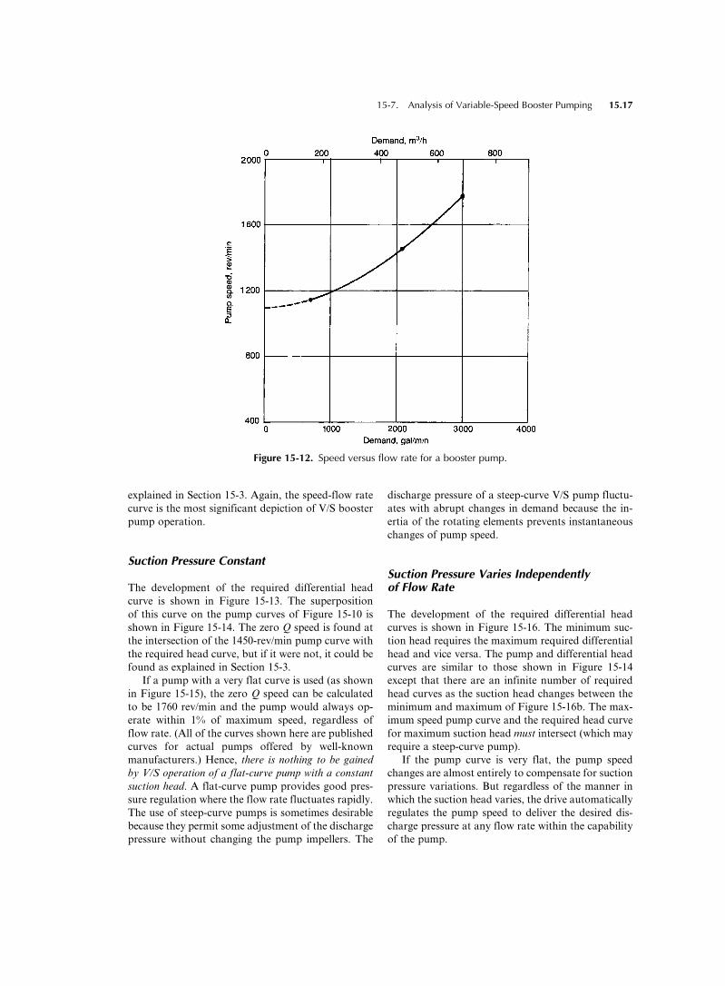
explained in Section 15-3. Again, the speed-flow rate

curve is the most significant depiction of V/S booster

pump operation.

Suction Pressure Constant

The development of the required differential head

curve is shown in Figure 15-13. The superposition

of this curve on the pump curves of Figure 15-10 is

shown in Figure 15-14. The zero Q speed is found at

the intersection of the 1450-rev/min pump curve with

the required head curve, but if it were not, it could be

found as explained in Section 15-3.

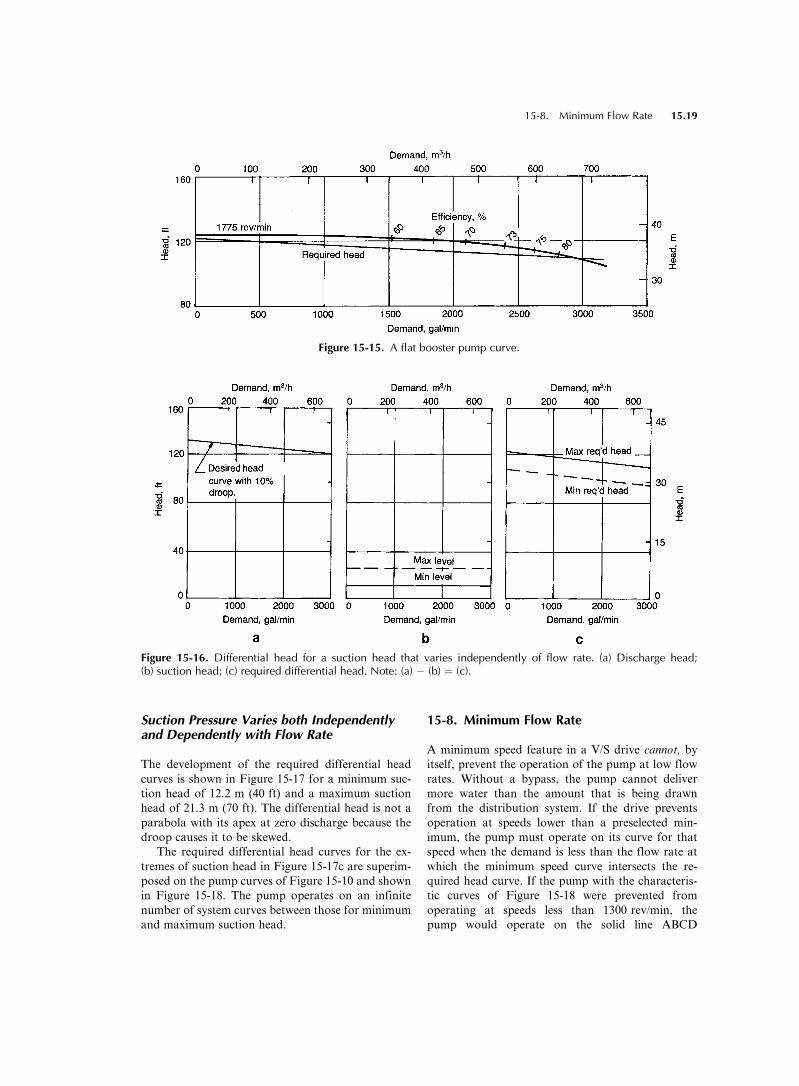
If a pump with a very flat curve is used (as shown

in Figure 15-15), the zero Q speed can be calculated

to be 1760 rev/min and the pump would always op-

erate within 1% of maximum speed, regardless of

flow rate. (All of the curves shown here are published

curves for actual pumps offered by well-known

manufacturers.) Hence, there is nothing to be gained

by V/S operation of a flat-curve pump with a constant

suction head. A flat-curve pump provides good pres-

sure regulation where the flow rate fluctuates rapidly.

The use of steep-curve pumps is sometimes desirable

because they permit some adjustment of the discharge

pressure without changing the pump impellers. The

discharge pressure of a steep-curve V/S pump fluctu-

ates with abrupt changes in demand because the in-

ertia of the rotating elements prevents instantaneous

changes of pump speed.

Suction Pressure Varies Independentlyof Flow Rate

The development of the required differential head

curves is shown in Figure 15-16. The minimum suc-

tion head requires the maximum required differential

head and vice versa. The pump and differential head

curves are similar to those shown in Figure 15-14

except that there are an infinite number of required

head curves as the suction head changes between the

minimum and maximum of Figure 15-16b. The max-

imum speed pump curve and the required head curve

for maximum suction head must intersect (which may

require a steep-curve pump).

If the pump curve is very flat, the pump speed

changes are almost entirely to compensate for suction

pressure variations. But regardless of the manner in

which the suction head varies, the drive automatically

regulates the pump speed to deliver the desired dis-

charge pressure at any flow rate within the capability

of the pump.

Figure 15-12. Speed versus flow rate for a booster pump.

15-7. Analysis of Variable-Speed Booster Pumping 15.17

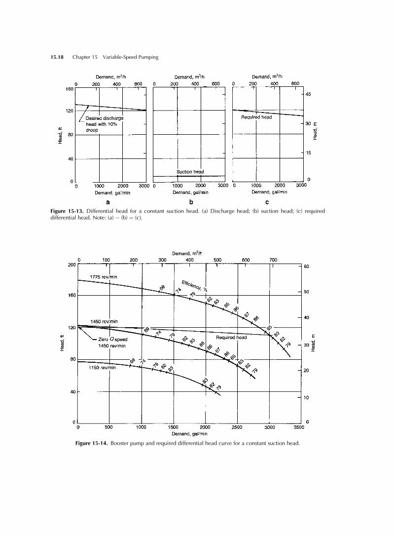
Figure 15-13. Differential head for a constant suction head. (a) Discharge head; (b) suction head; (c) requireddifferential head. Note: (a) � (b) ¼ (c).

Figure 15-14. Booster pump and required differential head curve for a constant suction head.

15.18 Chapter 15 Variable-Speed Pumping

Suction Pressure Varies both Independentlyand Dependently with Flow Rate

The development of the required differential head

curves is shown in Figure 15-17 for a minimum suc-

tion head of 12.2 m (40 ft) and a maximum suction

head of 21.3 m (70 ft). The differential head is not a

parabola with its apex at zero discharge because the

droop causes it to be skewed.

The required differential head curves for the ex-

tremes of suction head in Figure 15-17c are superim-

posed on the pump curves of Figure 15-10 and shown

in Figure 15-18. The pump operates on an infinite

number of system curves between those for minimum

and maximum suction head.

15-8. Minimum Flow Rate

A minimum speed feature in a V/S drive cannot, by

itself, prevent the operation of the pump at low flow

rates. Without a bypass, the pump cannot deliver

more water than the amount that is being drawn

from the distribution system. If the drive prevents

operation at speeds lower than a preselected min-

imum, the pump must operate on its curve for that

speed when the demand is less than the flow rate at

which the minimum speed curve intersects the re-

quired head curve. If the pump with the characteris-

tic curves of Figure 15-18 were prevented from

operating at speeds less than 1300 rev/min, the

pump would operate on the solid line ABCD

Figure 15-15. A flat booster pump curve.

Figure 15-16. Differential head for a suction head that varies independently of flow rate. (a) Discharge head;(b) suction head; (c) required differential head. Note: (a) � (b) ¼ (c).

15-8. Minimum Flow Rate 15.19

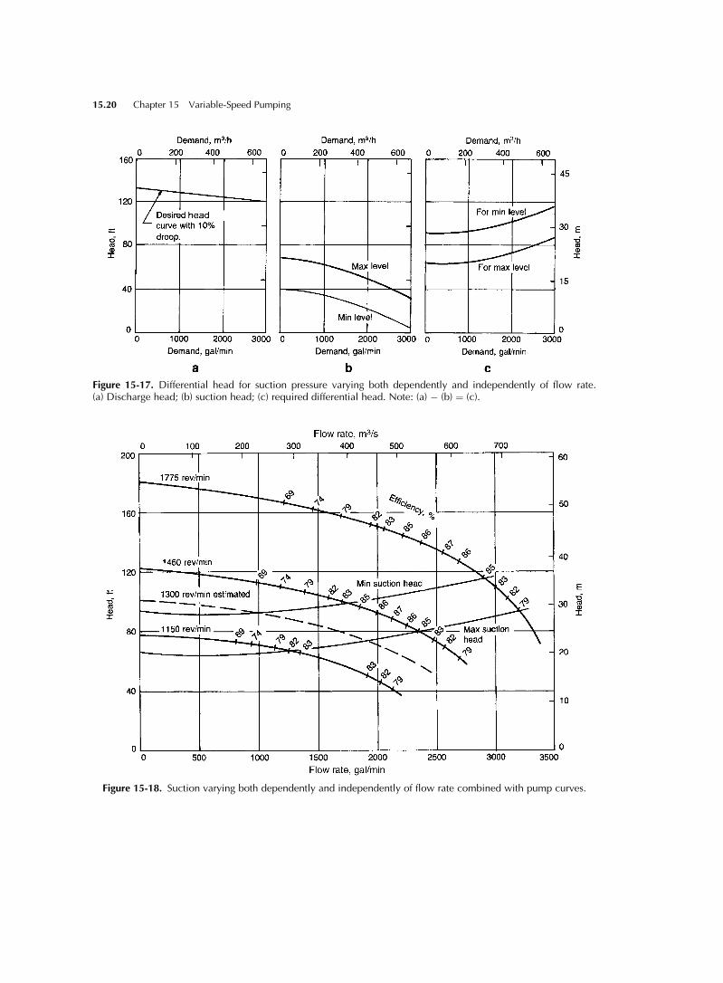
Figure 15-17. Differential head for suction pressure varying both dependently and independently of flow rate.(a) Discharge head; (b) suction head; (c) required differential head. Note: (a) � (b) ¼ (c).

Figure 15-18. Suction varying both dependently and independently of flow rate combined with pump curves.

15.20 Chapter 15 Variable-Speed Pumping

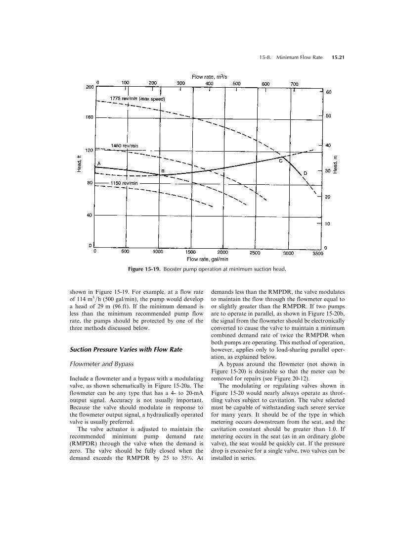
shown in Figure 15-19. For example, at a flow rate

of 114 m3=h (500 gal/min), the pump would develop

a head of 29 m (96 ft). If the minimum demand is

less than the minimum recommended pump flow

rate, the pumps should be protected by one of the

three methods discussed below.

Suction Pressure Varies with Flow Rate

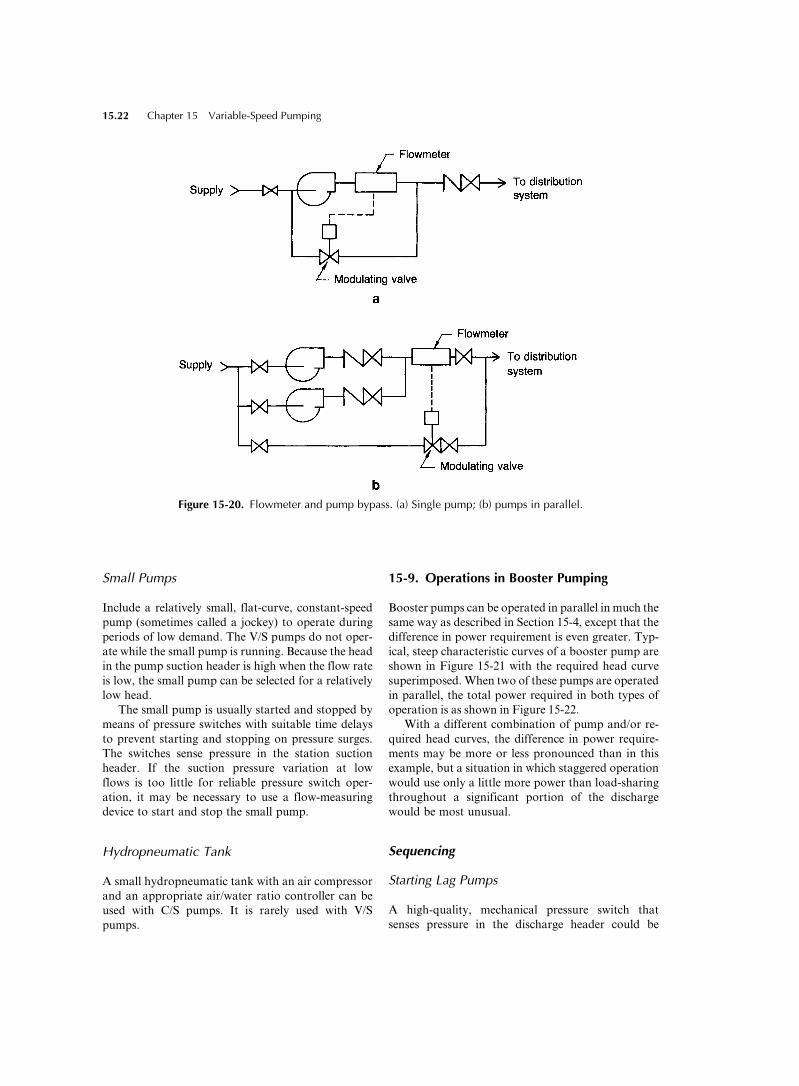
Flowmeter and Bypass

Include a flowmeter and a bypass with a modulating

valve, as shown schematically in Figure 15-20a. The

flowmeter can be any type that has a 4- to 20-mA

output signal. Accuracy is not usually important.

Because the valve should modulate in response to

the flowmeter output signal, a hydraulically operated

valve is usually preferred.

The valve actuator is adjusted to maintain the

recommended minimum pump demand rate

(RMPDR) through the valve when the demand is

zero. The valve should be fully closed when the

demand exceeds the RMPDR by 25 to 35%. At

demands less than the RMPDR, the valve modulates

to maintain the flow through the flowmeter equal to

or slightly greater than the RMPDR. If two pumps

are to operate in parallel, as shown in Figure 15-20b,

the signal from the flowmeter should be electronically

converted to cause the valve to maintain a minimum

combined demand rate of twice the RMPDR when

both pumps are operating. This method of operation,

however, applies only to load-sharing parallel oper-

ation, as explained below.

A bypass around the flowmeter (not shown in

Figure 15-20) is desirable so that the meter can be

removed for repairs (see Figure 20-12).

The modulating or regulating valves shown in

Figure 15-20 would nearly always operate as throt-

tling valves subject to cavitation. The valve selected

must be capable of withstanding such severe service

for many years. It should be of the type in which

metering occurs downstream from the seat, and the

cavitation constant should be greater than 1.0. If

metering occurs in the seat (as in an ordinary globe

valve), the seat would be quickly cut. If the pressure

drop is excessive for a single valve, two valves can be

installed in series.

Figure 15-19. Booster pump operation at minimum suction head.

15-8. Minimum Flow Rate 15.21

Small Pumps

Include a relatively small, flat-curve, constant-speed

pump (sometimes called a jockey) to operate during

periods of low demand. The V/S pumps do not oper-

ate while the small pump is running. Because the head

in the pump suction header is high when the flow rate

is low, the small pump can be selected for a relatively

low head.

The small pump is usually started and stopped by

means of pressure switches with suitable time delays

to prevent starting and stopping on pressure surges.

The switches sense pressure in the station suction

header. If the suction pressure variation at low

flows is too little for reliable pressure switch oper-

ation, it may be necessary to use a flow-measuring

device to start and stop the small pump.

Hydropneumatic Tank

A small hydropneumatic tank with an air compressor

and an appropriate air/water ratio controller can be

used with C/S pumps. It is rarely used with V/S

pumps.

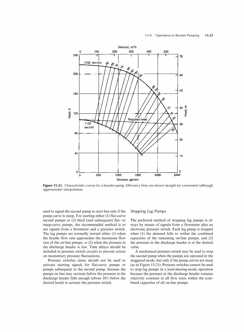
15-9. Operations in Booster Pumping

Booster pumps can be operated in parallel in much the

same way as described in Section 15-4, except that the

difference in power requirement is even greater. Typ-

ical, steep characteristic curves of a booster pump are

shown in Figure 15-21 with the required head curve

superimposed. When two of these pumps are operated

in parallel, the total power required in both types of

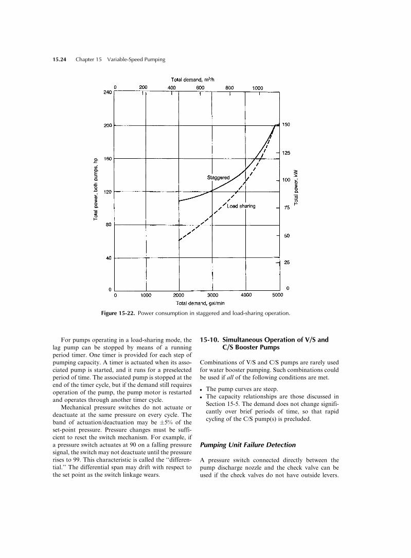
operation is as shown in Figure 15-22.

With a different combination of pump and/or re-

quired head curves, the difference in power require-

ments may be more or less pronounced than in this

example, but a situation in which staggered operation

would use only a little more power than load-sharing

throughout a significant portion of the discharge

would be most unusual.

Sequencing

Starting Lag Pumps

A high-quality, mechanical pressure switch that

senses pressure in the discharge header could be

Figure 15-20. Flowmeter and pump bypass. (a) Single pump; (b) pumps in parallel.

15.22 Chapter 15 Variable-Speed Pumping

used to signal the second pump to start but only if the

pump curve is steep. For starting either (1) flat-curve

second pumps or (2) third (and subsequent) flat- or

steep-curve pumps, the recommended method is to

use signals from a flowmeter and a pressure switch.

The lag pumps are normally started either (1) when

the header flow rate approaches the maximum flow

rate of the on-line pumps, or (2) when the pressure in

the discharge header is low. Time delays should be

included in pressure switch circuits to prevent action

on momentary pressure fluctuations.

Pressure switches alone should not be used to

activate starting signals for flat-curve pumps or

pumps subsequent to the second pump, because the

pumps on line may cavitate before the pressure in the

discharge header falls enough (about 10% below the

desired head) to actuate the pressure switch.

Stopping Lag Pumps

The preferred method of stopping lag pumps is al-

ways by means of signals from a flowmeter plus an

electronic pressure switch. Each lag pump is stopped

when (1) the demand falls to within the combined

capacities of the remaining on-line pumps, and (2)

the pressure in the discharge header is at the desired

value.

A mechanical pressure switch may be used to stop

the second pump when the pumps are operated in the

staggered mode, but only if the pump curves are steep

(as in Figure 15-21). Pressure switches cannot be used

to stop lag pumps in a load-sharing-mode operation

because the pressure in the discharge header remains

relatively constant at all flow rates within the com-

bined capacities of all on-line pumps.

Figure 15-21. Characteristic curves for a booster pump. Efficiency lines are shown straight for convenient (althoughapproximate) interpolation.

15-9. Operations in Booster Pumping 15.23

For pumps operating in a load-sharing mode, the

lag pump can be stopped by means of a running

period timer. One timer is provided for each step of

pumping capacity. A timer is actuated when its asso-

ciated pump is started, and it runs for a preselected

period of time. The associated pump is stopped at the

end of the timer cycle, but if the demand still requires

operation of the pump, the pump motor is restarted

and operates through another timer cycle.

Mechanical pressure switches do not actuate or

deactuate at the same pressure on every cycle. The

band of actuation/deactuation may be �5% of the

set-point pressure. Pressure changes must be suffi-

cient to reset the switch mechanism. For example, if

a pressure switch actuates at 90 on a falling pressure

signal, the switch may not deactuate until the pressure

rises to 99. This characteristic is called the ‘‘differen-

tial.’’ The differential span may drift with respect to

the set point as the switch linkage wears.

15-10. Simultaneous Operation of V/S andC/S Booster Pumps

Combinations of V/S and C/S pumps are rarely used

for water booster pumping. Such combinations could

be used if all of the following conditions are met.

. The pump curves are steep.

. The capacity relationships are those discussed in

Section 15-5. The demand does not change signifi-

cantly over brief periods of time, so that rapid

cycling of the C/S pump(s) is precluded.

Pumping Unit Failure Detection

A pressure switch connected directly between the

pump discharge nozzle and the check valve can be

used if the check valves do not have outside levers.

Figure 15-22. Power consumption in staggered and load-sharing operation.

15.24 Chapter 15 Variable-Speed Pumping

Pressure switches are useful and can detect all in-

ternal pumping unit failures, but they cannot detect

whether flow is occurring. Check valve limit switches

are always preferred to pressure switches.

Other Considerations

The special design considerations discussed in Section

15-6 apply equally well to booster pumping.

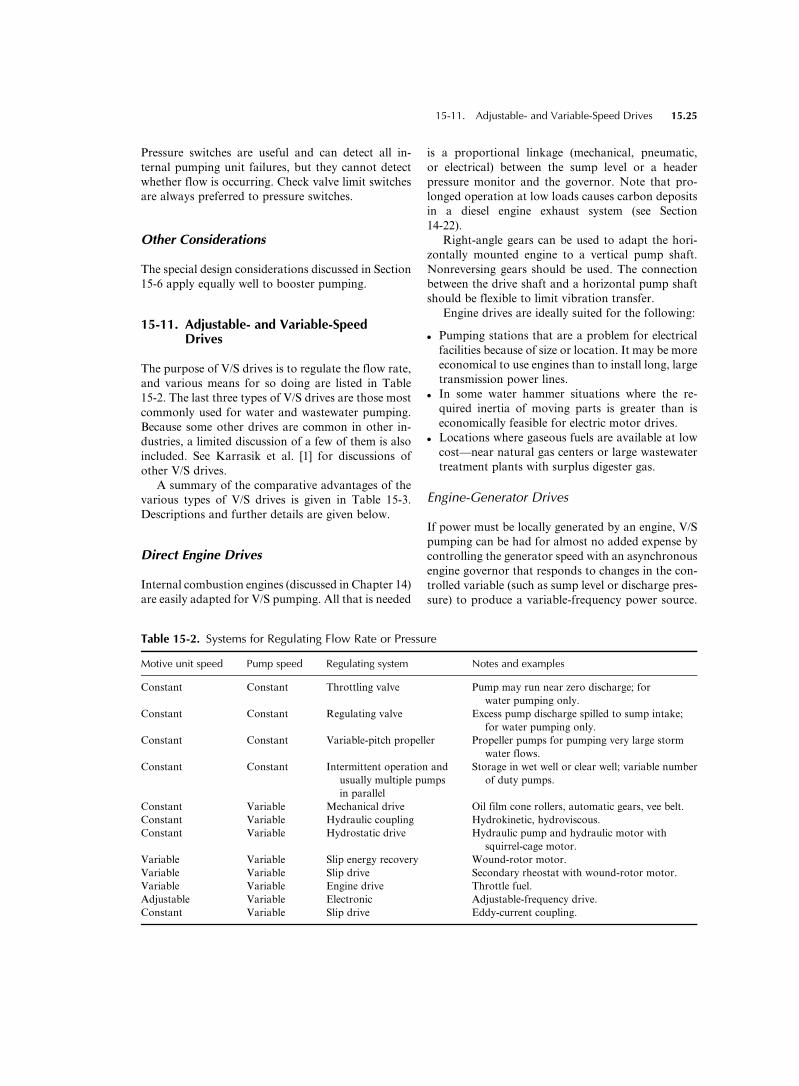
15-11. Adjustable- and Variable-SpeedDrives

The purpose of V/S drives is to regulate the flow rate,

and various means for so doing are listed in Table

15-2. The last three types of V/S drives are those most

commonly used for water and wastewater pumping.

Because some other drives are common in other in-

dustries, a limited discussion of a few of them is also

included. See Karrasik et al. [1] for discussions of

other V/S drives.

A summary of the comparative advantages of the

various types of V/S drives is given in Table 15-3.

Descriptions and further details are given below.

Direct Engine Drives

Internal combustion engines (discussed in Chapter 14)

are easily adapted for V/S pumping. All that is needed

is a proportional linkage (mechanical, pneumatic,

or electrical) between the sump level or a header

pressure monitor and the governor. Note that pro-

longed operation at low loads causes carbon deposits

in a diesel engine exhaust system (see Section

14-22).

Right-angle gears can be used to adapt the hori-

zontally mounted engine to a vertical pump shaft.

Nonreversing gears should be used. The connection

between the drive shaft and a horizontal pump shaft

should be flexible to limit vibration transfer.

Engine drives are ideally suited for the following:

. Pumping stations that are a problem for electrical

facilities because of size or location. It may be more

economical to use engines than to install long, large

transmission power lines.

. In some water hammer situations where the re-

quired inertia of moving parts is greater than is

economically feasible for electric motor drives.

. Locations where gaseous fuels are available at low

cost—near natural gas centers or large wastewater

treatment plants with surplus digester gas.

Engine-Generator Drives

If power must be locally generated by an engine, V/S

pumping can be had for almost no added expense by

controlling the generator speed with an asynchronous

engine governor that responds to changes in the con-

trolled variable (such as sump level or discharge pres-

sure) to produce a variable-frequency power source.

Table 15-2. Systems for Regulating Flow Rate or Pressure

Motive unit speed Pump speed Regulating system Notes and examples

Constant Constant Throttling valve Pump may run near zero discharge; for

water pumping only.

Constant Constant Regulating valve Excess pump discharge spilled to sump intake;

for water pumping only.

Constant Constant Variable-pitch propeller Propeller pumps for pumping very large storm

water flows.

Constant Constant Intermittent operation and

usually multiple pumps

in parallel

Storage in wet well or clear well; variable number

of duty pumps.

Constant Variable Mechanical drive Oil film cone rollers, automatic gears, vee belt.

Constant Variable Hydraulic coupling Hydrokinetic, hydroviscous.

Constant Variable Hydrostatic drive Hydraulic pump and hydraulic motor with

squirrel-cage motor.

Variable Variable Slip energy recovery Wound-rotor motor.

Variable Variable Slip drive Secondary rheostat with wound-rotor motor.

Variable Variable Engine drive Throttle fuel.

Adjustable Variable Electronic Adjustable-frequency drive.

Constant Variable Slip drive Eddy-current coupling.

15-11. Adjustable- and Variable-Speed Drives 15.25

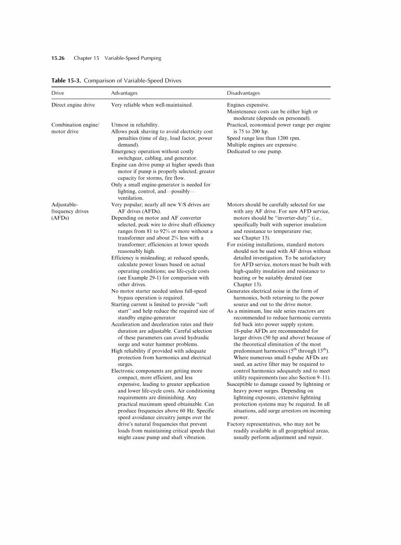
Table 15-3. Comparison of Variable-Speed Drives

Drive Advantages Disadvantages

Direct engine drive Very reliable when well-maintained. Engines expensive.

Maintenance costs can be either high or

moderate (depends on personnel).

Combination engine/

motor drive

Utmost in reliability.

Allows peak shaving to avoid electricity cost

penalties (time of day, load factor, power

demand).

Emergency operation without costly

switchgear, cabling, and generator.

Engine can drive pump at higher speeds than

motor if pump is properly selected; greater

capacity for storms, fire flow.

Only a small engine-generator is needed for

lighting, control, and—possibly—

ventilation.

Practical, economical power range per engine

is 75 to 200 hp.

Speed range less than 1200 rpm.

Multiple engines are expensive.

Dedicated to one pump.

Adjustable-

frequency drives

(AFDs)

Very popular; nearly all new V/S drives are

AF drives (AFDs).

Depending on motor and AF converter

selected, peak wire to drive shaft efficiency

ranges from 81 to 92% or more without a

transformer and about 2% less with a

transformer; efficiencies at lower speeds

reasonably high.

Efficiency is misleading; at reduced speeds,

calculate power losses based on actual

operating conditions; use life-cycle costs

(see Example 29-1) for comparison with

other drives.

No motor starter needed unless full-speed

bypass operation is required.

Starting current is limited to provide ‘‘soft

start’’ and help reduce the required size of

standby engine-generator

Acceleration and deceleration rates and their

duration are adjustable. Careful selection

of these parameters can avoid hydraulic

surge and water hammer problems.

High reliability if provided with adequate

protection from harmonics and electrical

surges.

Electronic components are getting more

compact, more efficient, and less

expensive, leading to greater application

and lower life-cycle costs. Air conditioning

requirements are diminishing. Any

practical maximum speed obtainable. Can

produce frequencies above 60 Hz. Specific

speed avoidance circuitry jumps over the

drive’s natural frequencies that prevent

loads from maintaining critical speeds that

might cause pump and shaft vibration.

Motors should be carefully selected for use

with any AF drive. For new AFD service,

motors should be ‘‘inverter-duty’’ (i.e.,

specifically built with superior insulation

and resistance to temperature rise;

see Chapter 13).

For existing installations, standard motors

should not be used with AF drives without

detailed investigation. To be satisfactory

for AFD service, motors must be built with

high-quality insulation and resistance to

heating or be suitably derated (see

Chapter 13).

Generates electrical noise in the form of

harmonics, both returning to the power

source and out to the drive motor.

As a minimum, line side series reactors are

recommended to reduce harmonic currents

fed back into power supply system.

18-pulse AFDs are recommended for

larger drives (50 hp and above) because of

the theoretical elimination of the most

predominant harmonics (5th through 13th).

Where numerous small 6-pulse AFDs are

used, an active filter may be required to

control harmonics adequately and to meet

utility requirements (see also Section 9–11).

Susceptible to damage caused by lightning or

heavy power surges. Depending on

lightning exposure, extensive lightning

protection systems may be required. In all

situations, add surge arrestors on incoming

power.

Factory representatives, who may not be

readily available in all geographical areas,

usually perform adjustment and repair.

15.26 Chapter 15 Variable-Speed Pumping

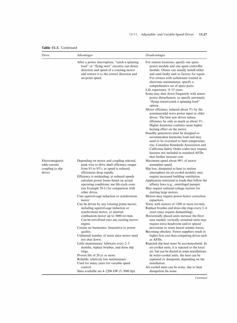
Table 15-3. Continued

Drive Advantages Disadvantages

After a power interruption, ‘‘catch a spinning

load’’ or ‘‘flying start’’ circuitry can detect

direction and speed of a coasting motor

and restore it to the correct direction and

set-point speed.

For remote locations, specify one spare

power module and one spare controller

module. Owner can usually install either

and send faulty unit to factory for repair.

For owners with technicians trained in

electronic maintenance, specify a

comprehensive set of spare parts.

Life expectancy: 8–15 years.

Some may shut down frequently with minor

power disturbances, so specify automatic

‘‘flying restart/catch a spinning load’’

option.

Motor efficiency reduced about 5% by the

nonsinusoidal wave power input in older

drives. The best new drives reduce

efficiency by only as much as about 3%.

Higher harmonic contents cause higher

heating effect on the motor.

Standby generators must be designed to

accommodate harmonic load and may

need to be oversized to limit temperature

rise. Canadian Standards Association and

California Safety Order codes may require

features not included in standard AFDs

that further increase cost.

Electromagnetic

eddy-current

coupling (a slip

drive)

Depending on motor and coupling selected,

peak wire to drive shaft efficiency ranges

from 83 to 93%; as speed is reduced,

efficiencies drop rapidly.

Efficiency is misleading; at reduced speeds

calculate power losses based on actual

operating conditions; use life-cycle costs

(see Example 29-1) for comparison with

other drives.

Uses squirrel-cage induction or synchronous

motor

Can be driven by any rotating prime mover,

including squirrel-cage induction or

synchronous motor, or internal

combustion motor up to 3600 rev/min.

Can be retrofitted onto any existing motor/

engine.

Creates no harmonics. Insensitive to power

quality.

Unlimited number of starts since motor need

not shut down.

Little maintenance: lubricate every 2–3

months, replace brushes, and dress slip

rings.

Proven life of 20 yr or more.

Reliable; relatively low maintenance.

Used for many years for variable speed

control.

Sizes available are 4–2200 kW (5–3000 hp).

Maximum speed about 98% of motor

nameplate speed.

Slip loss, dissipated as heat to station

atmosphere (in air-cooled models), may

require increased building ventilation.

Application restricted to loads that follow the

affinity laws (e.g., centrifugal pumps).

May require reduced-voltage starters for

starting large motors.

Motors may require power-factor correction

capacitors.

Noisy with motors of 1200 or more rev/min.

Replace brushes and dress slip rings every 2–4

years (may require dismantling).

Horizontally placed units increase the floor

area needed; vertically mounted units may

require extra headroom and/or special

provisions to resist lateral seismic forces.

Becoming obsolete. Fewer suppliers result in

higher first cost than competing drives such

as AFDs.

Rejected slip heat must be accommodated. In

air-cooled units, it is rejected to the local

air, but can be ducted in some installations.

In water-cooled units, the heat can be

captured or dissipated, depending on the

installation.

Air-cooled units can be noisy, due to heat

dissipation fin noise.

Continued

15-11. Adjustable- and Variable-Speed Drives 15.27

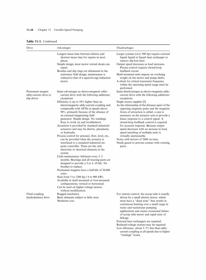
Table 15-3. Continued

Drive Advantages Disadvantages

Longest mean time between failures and

shortest mean time for repairs in most

places.

Simple design; most motor rewind shops can

repair.

Brushes and slip rings are eliminated in the

stationary field design; maintenance is

reduced to that of a squirrel-cage induction

motor.

Larger systems (over 500 hp) require external

liquid–liquid or liquid–heat exchanger to

remove slip-loss heat.

Output speed decreases as load increases.

Precise control requires closed-loop

feedback circuit.

Shaft-mounted units impose an overhung

weight on the motor and pump shafts.

A check for critical (resonant) frequency

within the operating speed range must be

performed.

Permanent magnet

eddy-current drive (a

slip drive)

Same advantages as electro-magnetic eddy-

current drive with the following additions/

exceptions:

Efficiency is up to 10% higher than an

electromagnetic eddy-current coupling and

comparable with AFDs at speeds above

90%, primarily because of the absence of

an external magnetizing field

generator. Simple design. No windings.

Easy to work on and troubleshoot.

Actuation is provided by standard industrial

actuators and may be electric, pneumatic,

or hydraulic.

Process control for pressure, flow, level, etc.,

can be provided when the actuator is

interfaced to a standard industrial set-

point controller. These are the only

electronic or electrical elements in the

system.

Little maintenance: lubricate every 2–3

months. Bearings and all wearing parts are

designed to provide a 5-yr L-10 life. No

brushes to replace.

Permanent magnets have a half-life of 20,000

years.

Sizes from 5 to 1200 hp ( 4 to 900 kW).

Available in shaft-mounted or foot-mounted

configurations, vertical or horizontal.

Can be used on higher-voltage motors

without modification.

Same disadvantages as electro-magnetic eddy-

current drive with the following additions/

exceptions:

Single source supplier [2].

As the relationship of the distance apart of the

opposing magnetic poles and the magnetic

forces of attraction is cubed, a cam is

necessary on the actuator arm to provide a

linear response to a control signal. A

closed-loop feedback control is required

for accurate response. Because output

speed decreases with an increase in load,

speed matching of multiple units is

virtually unattainable.

Noisy with motors of 3600 rev/min.

Needs guard to prevent contact with rotating

parts.

Fluid coupling

(hydrokinetic) drive

Rugged machinery.

Basic elements subject to little wear.

Moderate cost.

For remote control, the scoop tube is usually

driven by a small electric motor, which

must have a ‘‘dead zone’’ that results in

continuous hunting over a small range in

water and wastewater pumping

applications and causes occasional failure

of scoop tube motor and rapid wear of

linkage.

External heat exchangers are required.

Reduced-voltage starters may be required.

Low efficiency, about 5–7% less than eddy-

current coupling at all speeds due to higher

‘‘windage’’ losses.

15.28 Chapter 15 Variable-Speed Pumping

One or more pump motors can be powered by one

generator in load-sharing operation. With a back-up

engine-generator set (which is usually required any-

way), this system is very reliable.

Combination Drives

If the utmost in reliability is required of the standby

power system, consider using direct-drive standby en-

gines for duty and standby pumps instead of an en-

gine-generator set. For horizontal, split-case pumps,

themotor ismounted at one end of the pump shaft and

the engine is mounted through an automatic clutch at

the other end. If a vertical motor drives the pump, a

combination right-angle gear and automatic clutch is

available to provide a horizontal shaft for an engine

and a mount for a vertical motor.

If power fails, the duty engine is started and the

motor is allowed to spin freely. An interlock must

disconnect the motor from the power source when the

engine is started. When electric power is restored, the

pump must first slow to well below synchronous

speed and the engine must be disconnected before

the motor is energized. Energizing a spinning motor

might not harm it (unless it is spinning in reverse), but

energizing a spinning motor with its residual field

remaining from interrupted electrical power by con-

necting it to another, nonsynchronized power source

Table 15-3. Continued

Drive Advantages Disadvantages

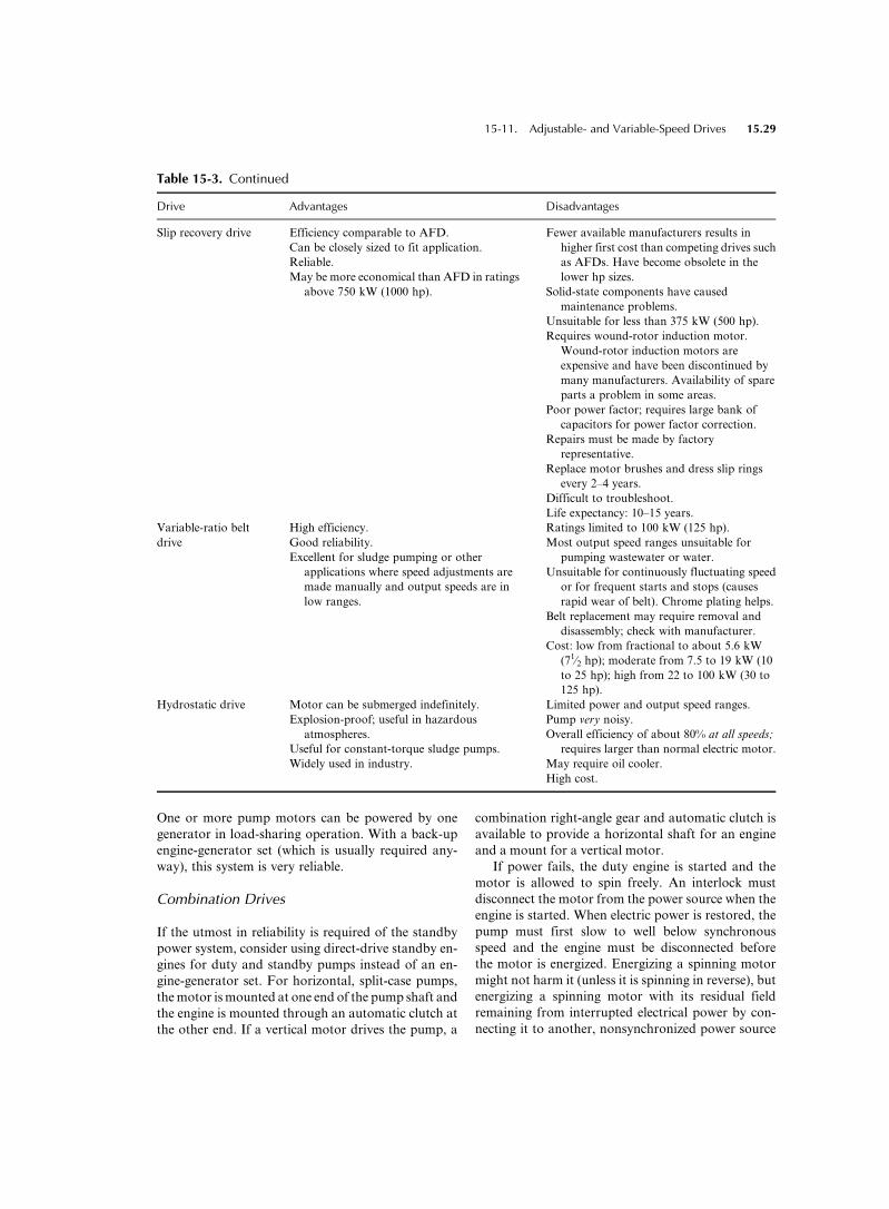
Slip recovery drive Efficiency comparable to AFD.

Can be closely sized to fit application.

Reliable.

May be more economical than AFD in ratings

above 750 kW (1000 hp).

Fewer available manufacturers results in

higher first cost than competing drives such

as AFDs. Have become obsolete in the

lower hp sizes.

Solid-state components have caused

maintenance problems.

Unsuitable for less than 375 kW (500 hp).

Requires wound-rotor induction motor.

Wound-rotor induction motors are

expensive and have been discontinued by

many manufacturers. Availability of spare

parts a problem in some areas.

Poor power factor; requires large bank of

capacitors for power factor correction.

Repairs must be made by factory

representative.

Replace motor brushes and dress slip rings

every 2–4 years.

Difficult to troubleshoot.

Life expectancy: 10–15 years.

Variable-ratio belt

drive

High efficiency.

Good reliability.

Excellent for sludge pumping or other

applications where speed adjustments are

made manually and output speeds are in

low ranges.

Ratings limited to 100 kW (125 hp).

Most output speed ranges unsuitable for

pumping wastewater or water.

Unsuitable for continuously fluctuating speed

or for frequent starts and stops (causes

rapid wear of belt). Chrome plating helps.

Belt replacement may require removal and

disassembly; check with manufacturer.

Cost: low from fractional to about 5.6 kW

(71⁄2 hp); moderate from 7.5 to 19 kW (10

to 25 hp); high from 22 to 100 kW (30 to

125 hp).

Hydrostatic drive Motor can be submerged indefinitely.

Explosion-proof; useful in hazardous

atmospheres.

Useful for constant-torque sludge pumps.

Widely used in industry.

Limited power and output speed ranges.

Pump very noisy.

Overall efficiency of about 80% at all speeds;

requires larger than normal electric motor.

May require oil cooler.

High cost.

15-11. Adjustable- and Variable-Speed Drives 15.29

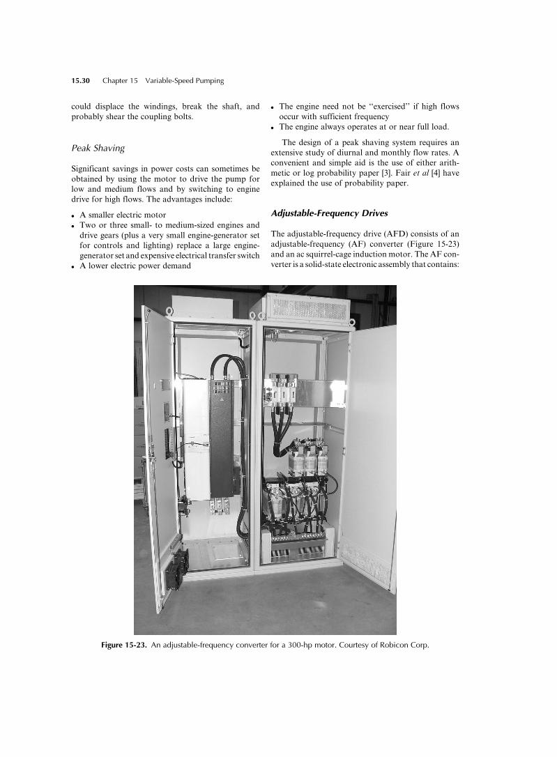
could displace the windings, break the shaft, and

probably shear the coupling bolts.

Peak Shaving

Significant savings in power costs can sometimes be

obtained by using the motor to drive the pump for

low and medium flows and by switching to engine

drive for high flows. The advantages include:

. A smaller electric motor

. Two or three small- to medium-sized engines and

drive gears (plus a very small engine-generator set

for controls and lighting) replace a large engine-

generator set and expensive electrical transfer switch

. A lower electric power demand

. The engine need not be ‘‘exercised’’ if high flows

occur with sufficient frequency

. The engine always operates at or near full load.

The design of a peak shaving system requires an

extensive study of diurnal and monthly flow rates. A

convenient and simple aid is the use of either arith-

metic or log probability paper [3]. Fair et al [4] have

explained the use of probability paper.

Adjustable-Frequency Drives

The adjustable-frequency drive (AFD) consists of an

adjustable-frequency (AF) converter (Figure 15-23)

and an ac squirrel-cage induction motor. The AF con-

verter is a solid-state electronic assembly that contains:

Figure 15-23. An adjustable-frequency converter for a 300-hp motor. Courtesy of Robicon Corp.

15.30 Chapter 15 Variable-Speed Pumping

. A rectifier, which converts incoming ac power to dc

power

. A filter to reduce the ripple in the dc power

. An inverter, which changes dc power to ac power

at any selected frequency within the design range.

A control signal from external equipment is sup-

plied to cause the inverter output frequency and volt-

age to vary as a function of some convenient variable,

such as pressure for water pumping or wet well liquid

level for wastewater pumping. The ac output of the

converter powers an ac squirrel-cage induction

motor, and the motor speed varies directly and lin-

early with the frequency of the applied power.

Almost all modern AF converters are pulse-width-

modulated (PWM) utilizing insulated gate bipolar

transistors (IGBTs) in the output stage, which produce

the output waveform shown in Figure 15-24c. Large

(over 450 kW or 600 hp at this time) AF converters

may use older thyristor designs that produce a stair-

step output or pulse-amplitude-modulated (PAM)

output (Figure 15-24a). The IGBT-type converter is

less expensive than older designs and produces an out-

put waveform that does not heat the motor as much as

PAM output. The disadvantages of the IGBT-type

are: (1) a very high switching frequency that results in

a high rate of change of voltage (dV/dt), and (2) high

peak voltages applied to the motor windings. Older-

type converters were frequently designated as either

(1) voltage source, or (2) current source. Voltage-

source converters (Figure 15-24a) have been replaced

by PWM converters for drives to 450 kW (600 hp).

The current-source type (Figure 15-24b) still has

adherents, is generally more expensive than voltage

source for a given horsepower, and is usually used

only for very large drives. As solid-state power tech-

nology advances, hybrid drives are now emerging.One

manufacturer makes a medium-voltage AF converter

using current-source topology with a PWM rectifier

front end and a matching inverter (i.e., called an

‘‘active front end.’’ This active front end drive is

claimed to produce near-sinusoidal output under all

load conditions and meets IEEE 519 limitations on

harmonic distortion regardless of system impedance.

Current-source convertersmust be closelymatched

to their load, but voltage-source converters can oper-

ate any sizemotor, evenmultiplemotors, as long as the

power requirement is within their rating. For drives

over 600 kW (800 hp), consider the medium-voltage

active front endAF converter or the load-commutated

converter, which either uses a synchronous motor or a

reactive output network to accomplish commutation.

Load-commutated converters are particularly suitable

for motors over 1500 kW (2000 hp).

Harmonics

All AFDs draw 5th, 7th, 11th, and 13th order harmonic

currents (300, 420, 660, 780 Hz, etc.) from a 60-Hz

Figure 15-24. Output waveforms from adjustable-frequency converters. (a) Voltage source six-step; (b)current source; (c) pulse-width modulated waveforms.Courtesy of Eaton Electric Drives Divisions.

15-11. Adjustable- and Variable-Speed Drives 15.31

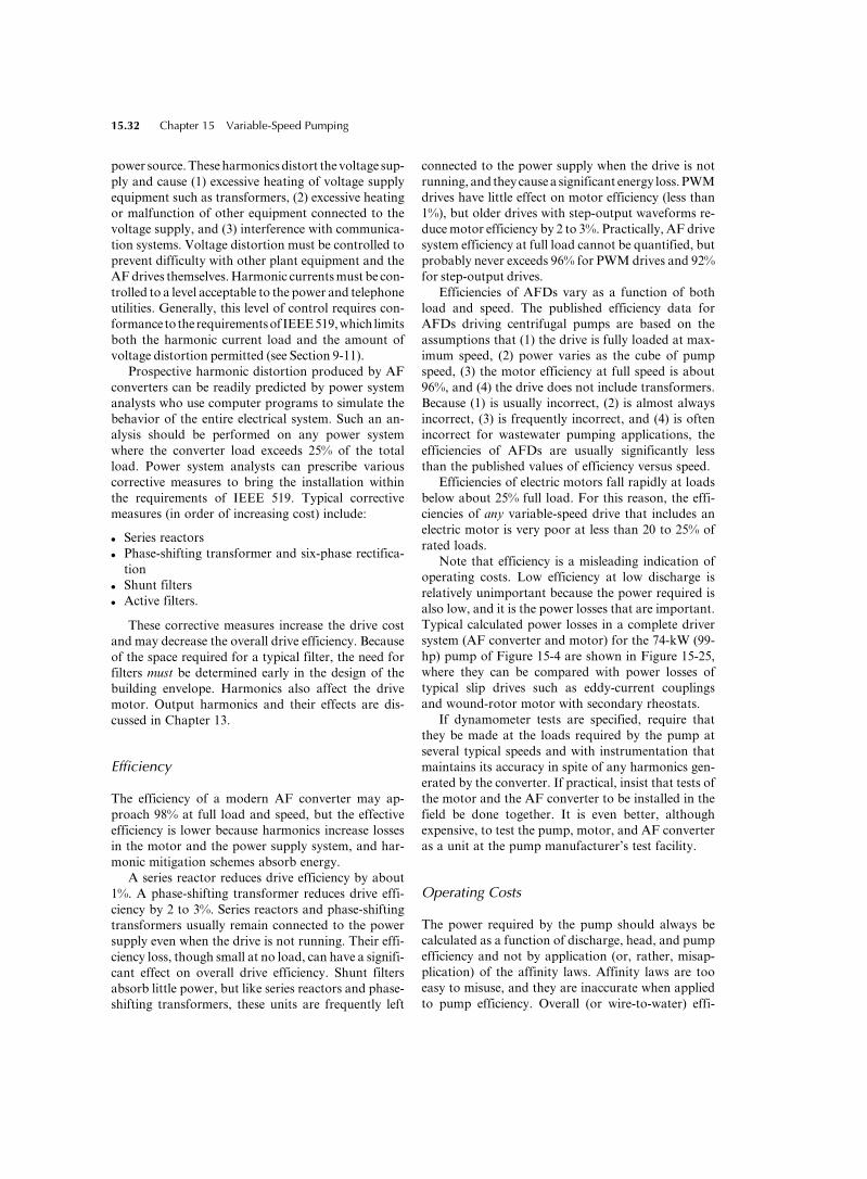
power source.Theseharmonics distort the voltage sup-

ply and cause (1) excessive heating of voltage supply

equipment such as transformers, (2) excessive heating

or malfunction of other equipment connected to the

voltage supply, and (3) interference with communica-

tion systems. Voltage distortion must be controlled to

prevent difficulty with other plant equipment and the

AFdrives themselves.Harmonic currentsmust be con-

trolled to a level acceptable to the power and telephone

utilities. Generally, this level of control requires con-

formancetotherequirementsof IEEE519,which limits

both the harmonic current load and the amount of

voltage distortion permitted (see Section 9-11).

Prospective harmonic distortion produced by AF

converters can be readily predicted by power system

analysts who use computer programs to simulate the

behavior of the entire electrical system. Such an an-

alysis should be performed on any power system

where the converter load exceeds 25% of the total

load. Power system analysts can prescribe various

corrective measures to bring the installation within

the requirements of IEEE 519. Typical corrective

measures (in order of increasing cost) include:

. Series reactors

. Phase-shifting transformer and six-phase rectifica-

tion

. Shunt filters

. Active filters.

These corrective measures increase the drive cost

and may decrease the overall drive efficiency. Because

of the space required for a typical filter, the need for

filters must be determined early in the design of the

building envelope. Harmonics also affect the drive

motor. Output harmonics and their effects are dis-

cussed in Chapter 13.

Efficiency

The efficiency of a modern AF converter may ap-

proach 98% at full load and speed, but the effective

efficiency is lower because harmonics increase losses

in the motor and the power supply system, and har-

monic mitigation schemes absorb energy.

A series reactor reduces drive efficiency by about

1%. A phase-shifting transformer reduces drive effi-

ciency by 2 to 3%. Series reactors and phase-shifting

transformers usually remain connected to the power

supply even when the drive is not running. Their effi-

ciency loss, though small at no load, can have a signifi-

cant effect on overall drive efficiency. Shunt filters

absorb little power, but like series reactors and phase-

shifting transformers, these units are frequently left

connected to the power supply when the drive is not

running, and they cause a significant energy loss. PWM

drives have little effect on motor efficiency (less than

1%), but older drives with step-output waveforms re-

ducemotor efficiency by 2 to 3%. Practically, AF drive

system efficiency at full load cannot be quantified, but

probably never exceeds 96% for PWMdrives and 92%

for step-output drives.

Efficiencies of AFDs vary as a function of both

load and speed. The published efficiency data for

AFDs driving centrifugal pumps are based on the

assumptions that (1) the drive is fully loaded at max-

imum speed, (2) power varies as the cube of pump

speed, (3) the motor efficiency at full speed is about

96%, and (4) the drive does not include transformers.

Because (1) is usually incorrect, (2) is almost always

incorrect, (3) is frequently incorrect, and (4) is often

incorrect for wastewater pumping applications, the

efficiencies of AFDs are usually significantly less

than the published values of efficiency versus speed.

Efficiencies of electric motors fall rapidly at loads

below about 25% full load. For this reason, the effi-

ciencies of any variable-speed drive that includes an

electric motor is very poor at less than 20 to 25% of

rated loads.

Note that efficiency is a misleading indication of

operating costs. Low efficiency at low discharge is

relatively unimportant because the power required is

also low, and it is the power losses that are important.

Typical calculated power losses in a complete driver

system (AF converter and motor) for the 74-kW (99-

hp) pump of Figure 15-4 are shown in Figure 15-25,

where they can be compared with power losses of

typical slip drives such as eddy-current couplings

and wound-rotor motor with secondary rheostats.

If dynamometer tests are specified, require that

they be made at the loads required by the pump at

several typical speeds and with instrumentation that

maintains its accuracy in spite of any harmonics gen-

erated by the converter. If practical, insist that tests of

the motor and the AF converter to be installed in the

field be done together. It is even better, although

expensive, to test the pump, motor, and AF converter

as a unit at the pump manufacturer’s test facility.

Operating Costs

The power required by the pump should always be

calculated as a function of discharge, head, and pump

efficiency and not by application (or, rather, misap-

plication) of the affinity laws. Affinity laws are too

easy to misuse, and they are inaccurate when applied

to pump efficiency. Overall (or wire-to-water) effi-

15.32 Chapter 15 Variable-Speed Pumping

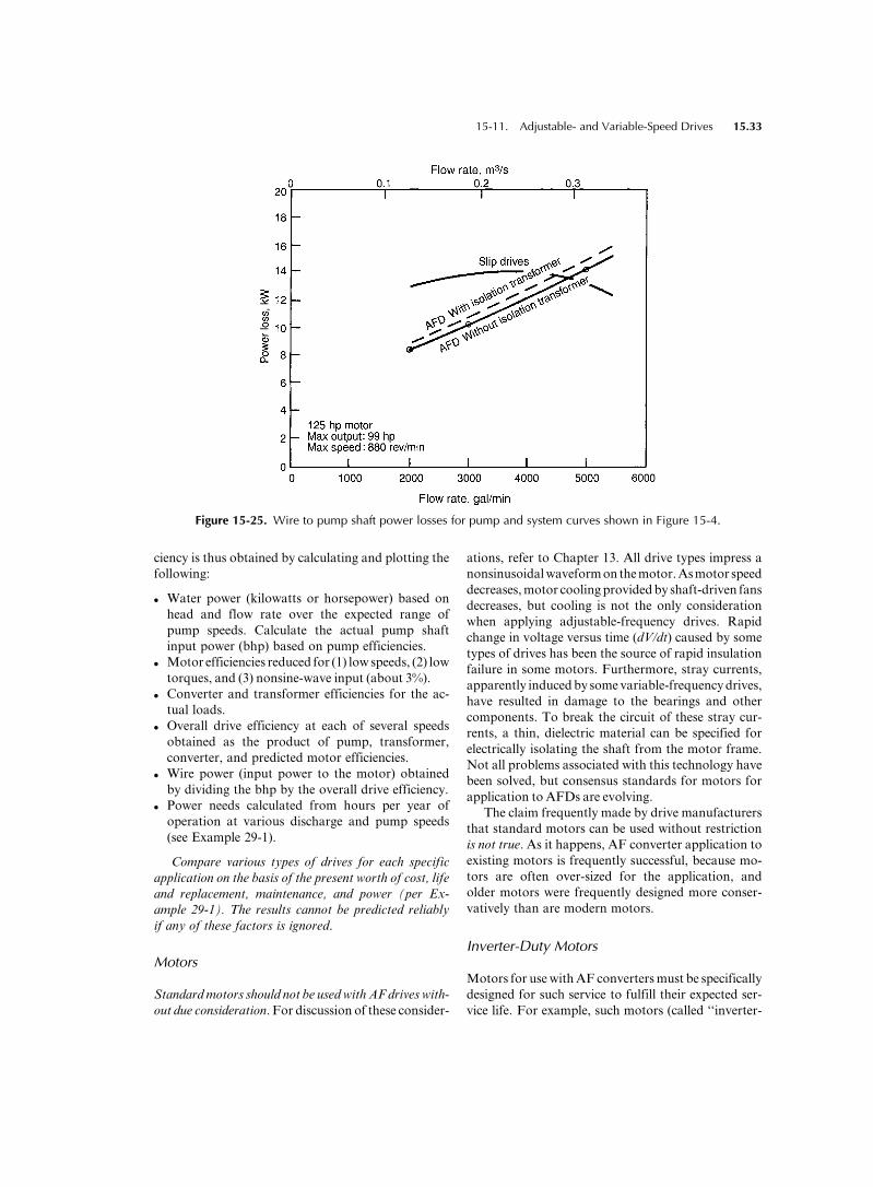
ciency is thus obtained by calculating and plotting the

following:

. Water power (kilowatts or horsepower) based on

head and flow rate over the expected range of

pump speeds. Calculate the actual pump shaft

input power (bhp) based on pump efficiencies.

. Motor efficiencies reduced for (1) low speeds, (2) low

torques, and (3) nonsine-wave input (about 3%).

. Converter and transformer efficiencies for the ac-

tual loads.

. Overall drive efficiency at each of several speeds

obtained as the product of pump, transformer,

converter, and predicted motor efficiencies.

. Wire power (input power to the motor) obtained

by dividing the bhp by the overall drive efficiency.

. Power needs calculated from hours per year of

operation at various discharge and pump speeds

(see Example 29-1).

Compare various types of drives for each specific

application on the basis of the present worth of cost, life

and replacement, maintenance, and power (per Ex-

ample 29-1). The results cannot be predicted reliably

if any of these factors is ignored.

Motors

Standardmotors should not be used with AF drives with-

out due consideration. For discussion of these consider-

ations, refer to Chapter 13. All drive types impress a

nonsinusoidalwaveformon themotor.Asmotor speed

decreases,motor coolingprovidedby shaft-driven fans

decreases, but cooling is not the only consideration

when applying adjustable-frequency drives. Rapid

change in voltage versus time (dV/dt) caused by some

types of drives has been the source of rapid insulation

failure in some motors. Furthermore, stray currents,

apparently inducedby somevariable-frequencydrives,

have resulted in damage to the bearings and other

components. To break the circuit of these stray cur-

rents, a thin, dielectric material can be specified for

electrically isolating the shaft from the motor frame.

Not all problems associated with this technology have

been solved, but consensus standards for motors for

application to AFDs are evolving.

The claim frequently made by drive manufacturers

that standard motors can be used without restriction

is not true. As it happens, AF converter application to

existing motors is frequently successful, because mo-

tors are often over-sized for the application, and

older motors were frequently designed more conser-

vatively than are modern motors.

Inverter-Duty Motors

Motors for usewithAF convertersmust be specifically

designed for such service to fulfill their expected ser-

vice life. For example, such motors (called ‘‘inverter-

Figure 15-25. Wire to pump shaft power losses for pump and system curves shown in Figure 15-4.

15-11. Adjustable- and Variable-Speed Drives 15.33

dutymotors’’) have stator wires double-dipped in var-

nish (wires in standardmotors are single-dipped); thin,

paper-like insulation is added in the slots; and Class H

or Class F insulation is used for Class B temperature

rise. The bearings are insulated from the motor frame

to interrupt stray currents and prevent electrolytic

corrosion. An option is grounding the rotor with a

brush connected to the frame. Inverter-duty motors

are about 15% more expensive than standard motors,

but they are more rugged and last much longer. For

that reason, it is often wise to specify them for solid-

state soft starters or even for across-the-line starter-

s. As always, proper grounding of the motor frame

and AF converter enclosure is essential. Be very con-

servative in specifying motors for use with AFDs.

In addition to the usual motor parameters that

must be specified when ordering an inverter duty

motor, the speed range and load speed/torque char-

acteristic must be specified. The motor manufac-

turer will then design the motor cooling for the

application. Motor manufacturers catalog their mo-

tors for speed ranges as great as 10:1 when driving

constant torque loads—a much more severe service

than driving a centrifugal pump over a typical 2:1

speed range and a load that varies geometrically with

speed.

Converters

Step-output converters and PWM converters that

do not use IGBT converters are generally satisfactory

with existing 1.15 service factor motors driving cen-

trifugal pumps if the motor is not loaded above the

nameplate rating (service factor not used). However,

both the foregoing AF converters are less efficient

and more expensive than modern converters.

IGBT converters switch their output at a very high

frequency (Figure 15-24b). They impress a high rate

of voltage change (dV/dt), and the switching action

also overshoots, thereby impressing high peak volt-

ages on the motor. Both characteristics put greater

stress on the motor insulation than does a sinusoidal

voltage. The motor insulation system must either be

designed for this stress, or other preventive measures

must be taken. Refer to Chapter 13. Definite-purpose

inverter-duty motors are preferred on all new AFD

installations. Always locate the AF converter as

close to the motor as possible. Long motor cable

runs (>45 m or 150 ft) magnify the peak voltages

produced by the AF converter. Output reactors are

recommended on all AFD installations employing

IGBT in the converter.

Operational Problems

Any short interruption of power (sufficient to make a

light flicker) can trip an older AFD, after which the

motor must be allowed to come to rest before restart-

ing—a requirement annoying in thunderstorms and

windstorms, which could cause several interruptions

per day. Most modern AFDs, however, are designed

to operate through such momentary (less than 0.5 s)

power losses, and AFDs can be designed to synchron-

ize with a spinning motor (this feature is called ‘‘catch

a spinning load’’ or ‘‘flying restart’’), but these fea-

tures must be specified if specifically wanted. They

increase the cost of the AFD only slightly, if at all.

Designing and/or specifying the interfacing be-

tween the motor and AF converter is not a simple

task. One way to promote compatibility is to specify

‘‘unit responsibility,’’ in which the pump, motor, con-

verter, and isolating transformer (if any) are all fur-

nished by one supplier (the pump manufacturer) who

has full responsibility for the proper operation of the

entire pumpingunit (seeChapter 16).Thepumpmanu-

facturer is in no position to warrant the compatibility

of the motor and the AF converter, so specify that the

entire power package be supplied to the pump manu-

facturer by the AFD manufacturer, who must ensure

the compatibility of the motor and the AF converter.

Because there are torsional pulsations in the output

of a motor powered by an AF converter, it is strongly

recommended that a torsional analysis be done for any

drive of more than 300 kW (400 hp). Vertical motors

supplied with variable-speed systems are subject to

‘‘reed frequency’’ vibration. The motor, the pump,

and the control manufacturers must coordinate to

eliminate this potential problem (see ‘‘Unit Responsi-

bility’’ in Appendix C). Certain speeds may have to be

blocked out of the variable-speed range. These speeds

must, of course, be passed through during drive accel-

eration and deceleration, but the drive must not be

allowed to linger there. This feature is often standard

in newAFDs and is known as critical frequency avoid-

ance. A second problem that can occur if there is an

anti-reversing ratchet in the drive shaft is that dwelling

at certain speeds can cause an oscillation about the

vertical axis, hammer the ratchet, and damage or

destroy it.

Adjustable-Frequency Drive Specifications

A summary of specifications and requirements for a

reliable, trouble-free AFD system includes:

. A power system analysis. A source-voltage range of

þ10%, �5% from nominal (usually 460 V) is

15.34 Chapter 15 Variable-Speed Pumping

specified in NEMA standards for AF drives. Most

electrical equipment is designed for þ10% from

nominal. If the plant electrical system cannot meet

the tighter tolerance required by AF drives, specify

the voltage range that the drive must accept.

. Voltage disturbances. Modern drives have micro-

processor controllers. These controllers are capable

of maintaining drive operation through short

power supply voltage sags and automatically

restarting the drive if the sag exceeds the hold-up

interval. Specify ‘‘flying restart.’’

. Grounding. Protect the microprocessors by specify-

ing a ground grid in which each electrode, when

isolated, has a maximum ground resistance of

2 ohms—a protection significantly better than

that specified in the NEC.

. Motor insulation and AFD compatibility. Static

power converters impose unusual stress on winding

insulation. Early insulation failure will occur if the

motor is not designed for this duty. For AFD duty,

specify inverter-duty motors. See Chapter 13.

. Drive tuning. To ensure optimum performance, the

AFD must be tuned to the motor and load charac-

teristics. Some modern drives have a ‘‘self-tuning’’

function that permits the drive to adjust some

parameters to motor characteristics, but no drive

can analyze load requirements. Specify that the

drive be set up by a factory-authorized technician.

Do not rely on contractor electricians to set up AF

controllers.

. Voltage-vector control. Vector control for standard

pumping applications is neither necessary nor

recommended for pumping stations. For best per-

formance in other applications, however, specify

drives with voltage-vector control to regulate both

voltage and frequency to produce a sine wave out-

put for optimum motor magnetization and per-

formance, but the added cost is not worthwhile

for pump drivers.

. Isolation. A contactor to disconnect a drive physic-

ally from the motor is not necessary, but consider

specifying contactors to isolate shunt filters when

the drive is not running. If the drive is equipped with

a phase-shifting transformer, specify a line contac-

tor to eliminate the transformer losses when the

drive is not running. Input isolation has the benefit

of isolating the AFD from line disturbances and

lightning damage when the drive is not in use (or

on standby).

. Harmonic currents. Power factor correction is not

required for PWM-type AF drives. Power factor

correction is not recommended on the other types

of AFDs. If power factor correction is required

because other loads on a power system have a

lower power factor, filter traps must be added to

keep harmonic currents out of the capacitors. A

power system analyst can design suitable trapped

capacitor schemes for power systems with AF

drives.

. A temperature-controlled environment. A maximum

ambient temperature of 408C (1048F) is specified in

NEMA standards. Unless the space is air condi-

tioned, the temperature requirement may not be

met. AF drives generate substantial heat. Specify

a realistic ambient temperature requirement. If the

space is to be air conditioned (mandatory in many

geographic areas), obtain realistic heat dissipation

(including heat from transformers) values for the

drive from the manufacturer, specify these as max-

imums, and transmit the value to the air condition-

ing system designer.

. Standby generators. If the drive must be powered

by a standby generator, harmonic currents drawn

by the drive must be reduced to a minimum or

the generator may need to be derated. Heavy har-

monic filtration with shunt filters may result in a

leading power factor. Use 18-phase rectification,

series input reactors, and/or active filters in prefer-

ence to shunt filters to reduce harmonics. Be

sure the generator is capable of handling the har-

monic current load and any leading power factor

resulting from any filters. Be aware that the gener-

ator must be oversized to meet these requirements.

. Atmosphere. AFDs require clean, dry, cool air.

Hydrogen sulfide in the atmosphere must be lim-

ited to 3 ppb or less. Place the air intake on the

upwind side of the building, and pass the air

through a filter of, for example, activated carbon.

. Noise. An annoying hum (sometimes an ear-pier-

cing, high-frequency screech) is generated by AF

controllers, and motors are also noisy, so consider

sound-absorbing walls and ceilings to reduce the

reverberation. IGBT controllers, however, are

quiet and emit only a slightly noticeable hum.

. Operational features. Modern AFDs offer a wide

variety of features. Listed below are the most com-

mon ones and are standard on most models:

? Control. Speed can be adjusted either locally

from a keyboard or a potentiometer, or remotely

froma computer or control station. The drive can

follow a 4–20 ma or 0–10 VDC analog or serial

speed reference signal and can switch between

them based upon a digital input or serial com-

mand. Input selectable speeds (minimum, max-

imum, etc.), each with its own acceleration and

deceleration rates, are included. Local stop/start

as well as remote start, with local mode selection

are also included.

15-11. Adjustable- and Variable-Speed Drives 15.35

? Critical Frequency Avoidance. Skipping fre-

quencies with adjustable windows enable the

drive to avoid operating at speeds that resonate

with the driven equipment.

? Power Loss Ride-Through. Extended power-

loss ride-through helps avoid nuisance trips dur-

ing brownouts or other outages.

? Automatic Restart. The drive can automatically

restart following a fault trip. The number of

restart attempts and the interval between them

are selectable.

? Flying or Spinning Restart. After a power inter-

ruption, a spinning restart feature can detect

direction and speed of a coasting motor and

allows the drive to restore it to the correct dir-

ection and then accelerate or decelerate to set-

point speed without tripping.

? Communication. Most popular industry-

standard serial protocols are available for com-

municating with a station automation system,

including Modbus RTU2, Devicenet2, Ether-

net2, and Profibus2.

In conclusion, power system design for AF drives

presents problems that have been largely ignored in

the past and have resulted in many unsatisfactory

installations. Modern AF drives and proper power

system design should result in a problem-free vari-

able-speed pumping system with a life-cycle cost

lower than that of any other V/S drive.

Standby Generators

The harmonics generated by the converter are fed

back to the standby generator and, unless the gener-

ator voltage regulators are specifically designed for

compatibility with the AFDs, the generator may not

operate correctly with the drive (i.e., the regulator

may follow the converter pulse firing). The generator

manufacturer must match the generator to the spe-

cific AFD to be used.

Maintenance

The problems of repairing AFDs are controversial.

Some manufacturers claim that diagnostics and plug-

in circuit boards make troubleshooting and most

repairs relatively easy. However, most circuit boards

are expensive, and untrained, nonelectrical personnel

should not touch them. Moreover, replacing a thyris-

tor requires a very skilled technician and the proper

tools. Modern AF converters are built in a modular

fashion, allowing for easier troubleshooting and re-

placement. A competent, factory-trained mainten-

ance electrician should be able to service AFDs if:

. Training in power electronics is available at start-

up and on a periodic basis.

. The proper tools are available.

. A spare of every type of printed circuit board and

power electronic component is kept on hand.

Many boards, even for different sizes of AFDs,

are the same, so the inventory may not have to be

large. (Circuit boards usually cost between $750

and $2500 each; the cost of repair is about half as

much.) However, power electronic components are

different for different sizes of drives. Another rea-

son for keeping spare circuit boards is that some

manufacturing firms continue to drop out of the

solid-state business, and orphan electronics boards

may be very costly to replace and slow in delivery.

. Routine maintenance is low and consists only of

keeping the equipment clean and all connections

tight.

Other manufacturers state that all but simple

problems require a factory-authorized technician,

who is sometimes accompanied by an electrical en-

gineer at a charge of about $700 per person-day,

portal-to-portal, plus travel time and expenses. Re-

pairs often take two or three days. A worst-case

scenario might be a day for travel and diagnosis, a

day waiting for parts, and a day for installation and

start-up, which could total $4000 or $5000. Troubles

might occur yearly, more often, or never. Typically,

one might expect no trouble at all for two or three

years after start-up, with only occasional problems

later. Note, incidentally, that one lightning strike can

zap all of the AFDs, so make sure that the station is

protected from lightning (see Section 8-5).

Some expert consultants with considerable and

lengthy experience have had nerve-wracking problems

with AFDs, and they approach decisions regarding

their use with reservations and caution—especially

for municipal projects. They point to the problem of

competition with industry in hiring and keeping

trained technicians and the difficulty in procuring

spare parts for public utilities, and they urge that

spares be included in the original bid package. Make

sure that no critical items are omitted.

The industry is now more mature than it was

15 years ago, the equipment continues to improve,

reliability is better than it was in the past, and new

components continue to reduce the price of AFDs.

The improvements, however, tend to make electronic

equipment obsolete and parts may become unavail-

able. It seems wise to plan on replacing electronic

equipment every 10 to 15 years, and this cost should

15.36 Chapter 15 Variable-Speed Pumping

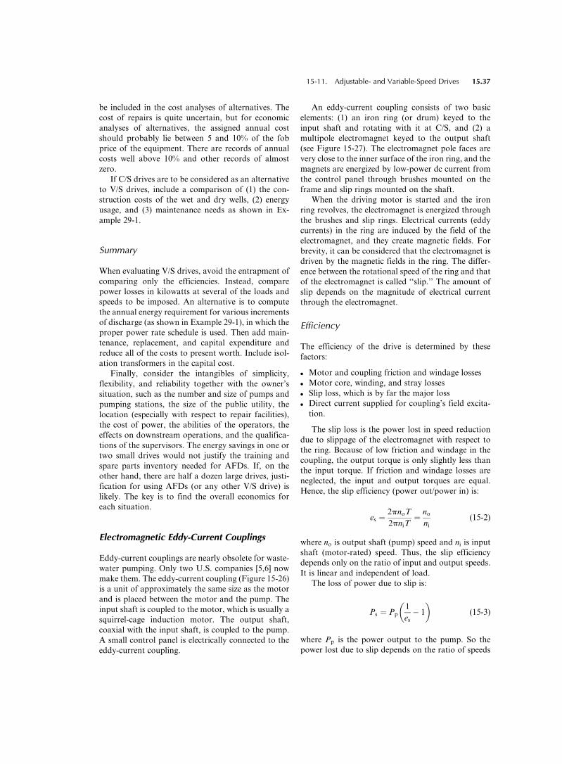
be included in the cost analyses of alternatives. The

cost of repairs is quite uncertain, but for economic

analyses of alternatives, the assigned annual cost

should probably lie between 5 and 10% of the fob

price of the equipment. There are records of annual

costs well above 10% and other records of almost

zero.

If C/S drives are to be considered as an alternative

to V/S drives, include a comparison of (1) the con-

struction costs of the wet and dry wells, (2) energy

usage, and (3) maintenance needs as shown in Ex-

ample 29-1.

Summary

When evaluating V/S drives, avoid the entrapment of

comparing only the efficiencies. Instead, compare

power losses in kilowatts at several of the loads and

speeds to be imposed. An alternative is to compute

the annual energy requirement for various increments

of discharge (as shown in Example 29-1), in which the

proper power rate schedule is used. Then add main-

tenance, replacement, and capital expenditure and

reduce all of the costs to present worth. Include isol-

ation transformers in the capital cost.

Finally, consider the intangibles of simplicity,

flexibility, and reliability together with the owner’s

situation, such as the number and size of pumps and

pumping stations, the size of the public utility, the

location (especially with respect to repair facilities),

the cost of power, the abilities of the operators, the

effects on downstream operations, and the qualifica-

tions of the supervisors. The energy savings in one or

two small drives would not justify the training and

spare parts inventory needed for AFDs. If, on the

other hand, there are half a dozen large drives, justi-

fication for using AFDs (or any other V/S drive) is

likely. The key is to find the overall economics for

each situation.

Electromagnetic Eddy-Current Couplings

Eddy-current couplings are nearly obsolete for waste-

water pumping. Only two U.S. companies [5,6] now

make them. The eddy-current coupling (Figure 15-26)

is a unit of approximately the same size as the motor

and is placed between the motor and the pump. The

input shaft is coupled to the motor, which is usually a

squirrel-cage induction motor. The output shaft,

coaxial with the input shaft, is coupled to the pump.

A small control panel is electrically connected to the

eddy-current coupling.

An eddy-current coupling consists of two basic

elements: (1) an iron ring (or drum) keyed to the

input shaft and rotating with it at C/S, and (2) a

multipole electromagnet keyed to the output shaft

(see Figure 15-27). The electromagnet pole faces are

very close to the inner surface of the iron ring, and the

magnets are energized by low-power dc current from

the control panel through brushes mounted on the

frame and slip rings mounted on the shaft.

When the driving motor is started and the iron

ring revolves, the electromagnet is energized through

the brushes and slip rings. Electrical currents (eddy

currents) in the ring are induced by the field of the

electromagnet, and they create magnetic fields. For

brevity, it can be considered that the electromagnet is

driven by the magnetic fields in the ring. The differ-

ence between the rotational speed of the ring and that

of the electromagnet is called ‘‘slip.’’ The amount of

slip depends on the magnitude of electrical current

through the electromagnet.

Efficiency

The efficiency of the drive is determined by these

factors:

. Motor and coupling friction and windage losses

. Motor core, winding, and stray losses

. Slip loss, which is by far the major loss

. Direct current supplied for coupling’s field excita-

tion.

The slip loss is the power lost in speed reduction

due to slippage of the electromagnet with respect to

the ring. Because of low friction and windage in the

coupling, the output torque is only slightly less than

the input torque. If friction and windage losses are

neglected, the input and output torques are equal.

Hence, the slip efficiency (power out/power in) is:

es ¼ 2pnoT

2pniT¼ no

ni(15-2)

where no is output shaft (pump) speed and ni is input

shaft (motor-rated) speed. Thus, the slip efficiency

depends only on the ratio of input and output speeds.

It is linear and independent of load.

The loss of power due to slip is:

Ps ¼ Pp

1

es� 1

� �(15-3)

where Pp is the power output to the pump. So the

power lost due to slip depends on the ratio of speeds

15-11. Adjustable- and Variable-Speed Drives 15.37

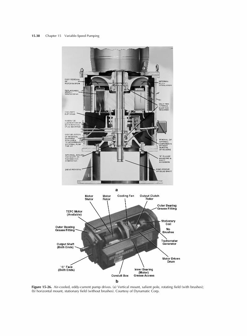
Figure 15-26. Air-cooled, eddy-current pump drives. (a) Vertical mount, salient pole, rotating field (with brushes);(b) horizontal mount, stationary field (without brushes). Courtesy of Dynamatic Corp.

15.38 Chapter 15 Variable-Speed Pumping

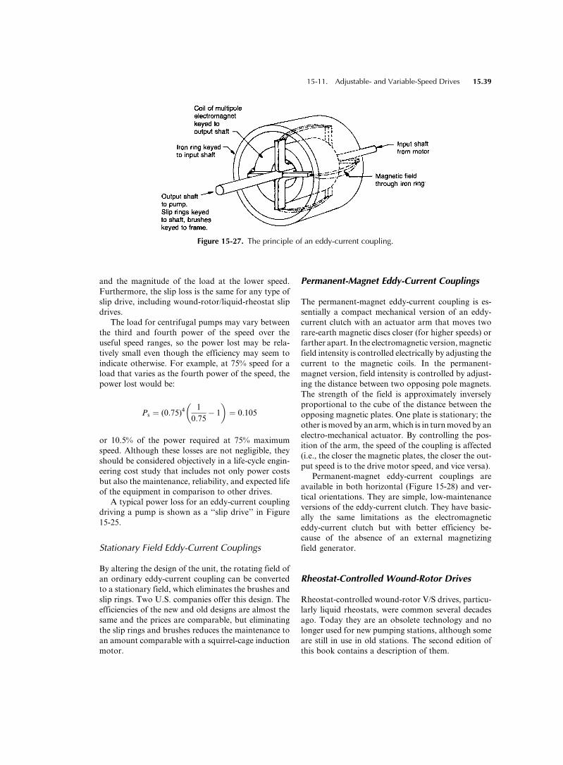
and the magnitude of the load at the lower speed.

Furthermore, the slip loss is the same for any type of

slip drive, including wound-rotor/liquid-rheostat slip

drives.

The load for centrifugal pumps may vary between

the third and fourth power of the speed over the

useful speed ranges, so the power lost may be rela-

tively small even though the efficiency may seem to

indicate otherwise. For example, at 75% speed for a

load that varies as the fourth power of the speed, the

power lost would be:

Ps ¼ (0:75)41

0:75� 1

� �¼ 0:105

or 10.5% of the power required at 75% maximum

speed. Although these losses are not negligible, they

should be considered objectively in a life-cycle engin-

eering cost study that includes not only power costs

but also the maintenance, reliability, and expected life

of the equipment in comparison to other drives.

A typical power loss for an eddy-current coupling

driving a pump is shown as a ‘‘slip drive’’ in Figure

15-25.

Stationary Field Eddy-Current Couplings

By altering the design of the unit, the rotating field of

an ordinary eddy-current coupling can be converted

to a stationary field, which eliminates the brushes and

slip rings. Two U.S. companies offer this design. The

efficiencies of the new and old designs are almost the

same and the prices are comparable, but eliminating

the slip rings and brushes reduces the maintenance to

an amount comparable with a squirrel-cage induction

motor.

Permanent-Magnet Eddy-Current Couplings

The permanent-magnet eddy-current coupling is es-

sentially a compact mechanical version of an eddy-

current clutch with an actuator arm that moves two

rare-earth magnetic discs closer (for higher speeds) or

farther apart. In the electromagnetic version,magnetic

field intensity is controlled electrically by adjusting the

current to the magnetic coils. In the permanent-

magnet version, field intensity is controlled by adjust-

ing the distance between two opposing pole magnets.

The strength of the field is approximately inversely

proportional to the cube of the distance between the

opposing magnetic plates. One plate is stationary; the

other ismoved by an arm,which is in turnmoved by an

electro-mechanical actuator. By controlling the pos-

ition of the arm, the speed of the coupling is affected

(i.e., the closer the magnetic plates, the closer the out-

put speed is to the drive motor speed, and vice versa).

Permanent-magnet eddy-current couplings are

available in both horizontal (Figure 15-28) and ver-

tical orientations. They are simple, low-maintenance

versions of the eddy-current clutch. They have basic-

ally the same limitations as the electromagnetic

eddy-current clutch but with better efficiency be-

cause of the absence of an external magnetizing

field generator.

Rheostat-Controlled Wound-Rotor Drives

Rheostat-controlled wound-rotor V/S drives, particu-

larly liquid rheostats, were common several decades

ago. Today they are an obsolete technology and no

longer used for new pumping stations, although some

are still in use in old stations. The second edition of

this book contains a description of them.

Figure 15-27. The principle of an eddy-current coupling.

15-11. Adjustable- and Variable-Speed Drives 15.39

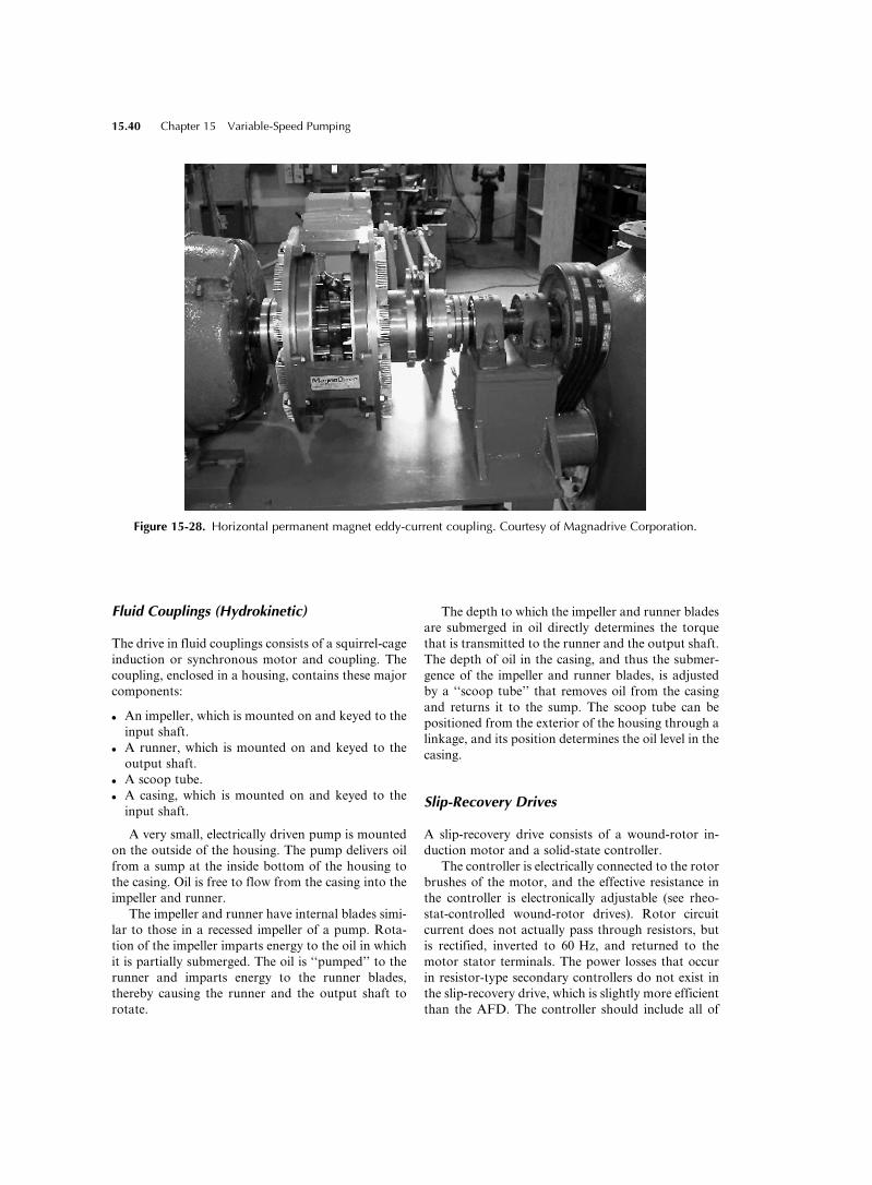
Fluid Couplings (Hydrokinetic)

The drive in fluid couplings consists of a squirrel-cage

induction or synchronous motor and coupling. The

coupling, enclosed in a housing, contains these major

components:

. An impeller, which is mounted on and keyed to the

input shaft.

. A runner, which is mounted on and keyed to the

output shaft.

. A scoop tube.

. A casing, which is mounted on and keyed to the

input shaft.

A very small, electrically driven pump is mounted

on the outside of the housing. The pump delivers oil

from a sump at the inside bottom of the housing to

the casing. Oil is free to flow from the casing into the

impeller and runner.

The impeller and runner have internal blades simi-

lar to those in a recessed impeller of a pump. Rota-

tion of the impeller imparts energy to the oil in which

it is partially submerged. The oil is ‘‘pumped’’ to the

runner and imparts energy to the runner blades,

thereby causing the runner and the output shaft to

rotate.

The depth to which the impeller and runner blades

are submerged in oil directly determines the torque

that is transmitted to the runner and the output shaft.

The depth of oil in the casing, and thus the submer-

gence of the impeller and runner blades, is adjusted

by a ‘‘scoop tube’’ that removes oil from the casing

and returns it to the sump. The scoop tube can be

positioned from the exterior of the housing through a

linkage, and its position determines the oil level in the

casing.

Slip-Recovery Drives

A slip-recovery drive consists of a wound-rotor in-

duction motor and a solid-state controller.

The controller is electrically connected to the rotor

brushes of the motor, and the effective resistance in

the controller is electronically adjustable (see rheo-

stat-controlled wound-rotor drives). Rotor circuit

current does not actually pass through resistors, but

is rectified, inverted to 60 Hz, and returned to the

motor stator terminals. The power losses that occur

in resistor-type secondary controllers do not exist in

the slip-recovery drive, which is slightly more efficient

than the AFD. The controller should include all of

Figure 15-28. Horizontal permanent magnet eddy-current coupling. Courtesy of Magnadrive Corporation.

15.40 Chapter 15 Variable-Speed Pumping

the necessary capacitors for power factor correction

and all of the circuit breakers required for line dis-

connect.

Variable-Ratio Belt Drives

The variable-ratio belt drive consists of a squirrel-

cage induction motor and two variable-pitch sheaves

with a belt, shafting, bearings, a sheave-pitch-chan-

ging mechanism, and a large spring, all of which are

enclosed in a housing.

One sheave (input) is either on a shaft directly

coupled to the motor shaft or mounted on an

extended motor shaft. The second sheave is mounted

on the output shaft. Power is transmitted from

the input to output sheaves by a heavy-duty vee-

belt.

Output shaft speed changes are accomplished by

changing the effective diameters of the sheave hubs

by changing the spacing between the sheave discs.

The discs are inside-tapered so moving one disc

(along the shaft) closer to the other disc of the sheave

forces the belt to engage the disc at a greater distance

from the hub. The position of one disc on the input

sheave is changed by an external linkage. The pos-

ition of the disc of the output sheave is changed by an

internal spring to keep belt tension relatively constant

regardless of changes in output speed. The discs

should be chrome-plated to reduce wear.

Hydrostatic Drives

A hydrostatic drive consists of the following:

. A squirrel-cage induction motor

. An adjustable displacement, multi-cylinder hy-

draulic pump

. A fixed displacement, multi-cylinder hydraulic

motor

. An oil reservoir.

The hydraulic pump is flexibly coupled to the ac

motor, and its shaft turns at C/S. The cylinder block

(which is cylindrical in shape) is keyed to the shaft

and contains the pistons. The entire assembly rotates

with the shaft. The piston rods bear and slide on a

‘‘swashplate’’ that does not rotate. The swashplate

can be tilted by an external device (through a linkage)

to change the effective displacement of the pump.

The hydraulic motor is connected to the hydraulic

pump by means of two hoses. The output of the

pump is circulated through the motor and back to

the pump intake. The shaft of the hydraulic motor is

flexibly coupled to the load shaft. The motor con-

struction is similar to the pump, except that its swash-

plate tilt is fixed. The motor output is connected to

the shaft of the wastewater pump. Changing the

swashplate angle changes the discharge rate of the

hydraulic pump, thus controlling the speed at which

the motor turns.

Refer to Table 15-3 for comparative advantages of

hydrostatic drives.

Other Drives

Other drives are available but are not described here

because they are not widely used for pumping water

or wastewater. Obviously, this situation may change,

so be alert to new products. Many types of rotating

machinery that are quite satisfactory for some spe-

cific use, however, are unsuitable for municipal

pumping. Be cautious in applying a new product by

making a thorough investigation of installations and

their maintenance records.

15-12. References

1. Karrasik, I. J., J. P. Messina, P. Cooper, and C. C. Heald,

Pump Handbook, 3rd ed., McGraw-Hill, New York

(2001).

2. MagnaDrive Corp., Seattle, WA.

3. Davis, C. V., and K. E. Sorensen, Handbook of Applied

Hydraulics, McGraw-Hill, New York (1969), pp. 40–16.

4. Fair, G. M., J. C. Geyer, and D. A. Okun, Water and

Wastewater Engineering, Vol. 1, Water Supply andWaste-

water Removal, John Wiley, New York (1966).

5. Ideal Electric Co., Mansfield, OH.

6. Electric Machinery Co., Inc., Minneapolis, MN.

7. DSI—Dynamatic, Inc., Sturtevant, WI.

15-12. References 15.41