Protection Against Reconstruction and Its Applications in Private

Federated Learning

Abhishek Bhowmick1, John Duchi1,2, Julien Freudiger1, Gaurav Kapoor1, and RyanRogers1

1ML Privacy Team, Apple, Inc.2Stanford University

Abstract

In large-scale statistical learning, data collection and model fitting are moving increasinglytoward peripheral devices—phones, watches, fitness trackers—away from centralized data collec-tion. Concomitant with this rise in decentralized data are increasing challenges of maintainingprivacy while allowing enough information to fit accurate, useful statistical models. This mo-tivates local notions of privacy—most significantly, local differential privacy, which providesstrong protections against sensitive data disclosures—where data is obfuscated before a statisti-cian or learner can even observe it, providing strong protections to individuals’ data. Yet localprivacy as traditionally employed may prove too stringent for practical use, especially in modernhigh-dimensional statistical and machine learning problems. Consequently, we revisit the typesof disclosures and adversaries against which we provide protections, considering adversaries withlimited prior information and ensuring that with high probability, ensuring they cannot recon-struct an individual’s data within useful tolerances. By reconceptualizing these protections, weallow more useful data release—large privacy parameters in local differential privacy—and wedesign new (minimax) optimal locally differentially private mechanisms for statistical learningproblems for all privacy levels. We thus present practicable approaches to large-scale locallyprivate model training that were previously impossible, showing theoretically and empiricallythat we can fit large-scale image classification and language models with little degradation inutility.

1 Introduction

New, more powerful computational hardware and access to substantial amounts of data has madefitting accurate models for image classification, text translation, physical particle prediction, astro-nomical observation, and other predictive tasks possible with previously infeasible accuracy [7, 2,49]. In many modern applications, data comes from measurements on small-scale devices with lim-ited computation and communication ability—remote sensors, phones, fitness monitors—makingfitting large scale predictive models both computationally and statistically challenging. Moreover,as more modes of data collection and computing move to peripherals—watches, power-metering,internet-enabled home devices, even lightbulbs—issues of privacy become ever more salient.

Such large-scale data collection motivates substantial work. Stochastic gradient methods arenow the de facto approach to large-scale model-fitting [70, 15, 60, 29], and recent work of McMahanet al. [54] describes systems (which they term federated learning) for aggregating multiple stochasticmodel-updates from distributed mobile devices. Yet even if only updates to a model are transmitted,

1

arX

iv:1

812.

0098

4v2

[st

at.M

L]

3 J

un 2

019

leaving all user or participant data on user-owned devices, it is easy to compromise the privacy ofusers [37, 56]. To see why this issue arises, consider any generalized linear model based on a datavector x, target y, and with loss of the form `(θ;x, y) = φ(〈θ, x〉, y). Then ∇θ`(θ;x, y) = c · x forsome c ∈ R, a scalar multiple of the user’s clear data x—a clear compromise of privacy. In thispaper, we describe an approach to fitting such large-scale models both privately and practically.

A natural approach to addressing the risk of information disclosure is to use differential pri-vacy [35], in which one defines a mechanism M , a randomized mapping from a sample xxx of datapoints to some space Z, which is ε-differentially private if

P(M(xxx) ∈ S)

P(M(xxx′) ∈ S)≤ eε (1)

for all samples xxx and xxx′ differing in at most one entry. Because of its strength and protectionproperties, differential privacy and its variants are the standard privacy definition in data analysisand machine learning [19, 32, 22]. Nonetheless, implementing such an algorithm presumes a levelof trust between users and a centralized data analyst, which may be undesirable or even untenable,as the data analyst has essentially unfettered access to a user’s data. Another approach to protect-ing individual updates is to use secure multiparty computation (SMC), sometimes in conjunctionwith differential privacy protections [14]. Traditional approaches to SMC require substantial com-munication and computation, making them untenable for large-scale data collection schemes, andBonawitz et al. [14] address a number of these, though individual user communication and compu-tation still increases with the number of users submitting updates and requires multiple rounds ofcommunication, which may be unrealistic when estimating models from peripheral devices.

An alternative to these approaches is to use locally private algorithms [67, 36, 31], in which anindividual keeps his or her data private even from the data collector. Such scenarios are natural indistributed (or federated) learning scenarios, where individuals provide data from their devices [53,3] but wish to maintain privacy. In our learning context, where a user has data x ∈ X that he orshe wishes to remain private, a randomized mechanism M : X → Z is ε-local differentially privateif for all x, x′ ∈ X and sets S ⊂ Z,

P(M(x) ∈ S)

P(M(x′) ∈ S)≤ eε. (2)

Roughly, a mechanism satisfying inequality (2) guarantees that even if an adversary knows thatthe initial data is one of x or x′, the adversary cannot distinguish them given an outcome Z (theprobability of error must be at least 1/(1 + eε)) [68]. Taking as motivation this testing definition,the “typical” recommendation for the parameter ε is to take ε as a small constant [68, 35, 32].

Local privacy protections provide numerous benefits: they allow easier compliance with reg-ulatory strictures, reduce risks (such as hacking) associated with maintaining private data, andallow more transparent protection of user privacy, because unprotected private data never leavesan individual’s device. Yet substantial work in the statistics, machine learning, and computerscience communities has shown that local differential privacy and its relaxations cause nontrivialchallenges for learning systems. Indeed, Duchi, Jordan, and Wainwright [30, 31] and Duchi andRogers [26] show that in a minimax (worst case population distribution) sense, learning with localdifferential privacy must suffer a degradation in sample complexity that scales as d/minε, ε2,where d is the dimension of the problem; taking ε as a small constant here suggests that estima-tion in problems of even moderate dimension will be challenging. Duchi and Ruan [27] develop acomplementary approach, arguing that a worst-case analysis is too conservative and may not accu-rately reflect the difficulty of problem instances one actually encounters, so that an instance-specifictheory of optimality is necessary. In spite of this instance-specific optimality theory for locally pri-vate procedures—that is, fundamental limits on learning that apply to the particular problem at

2

hand—Duchi and Ruan’s results suggest that local notions of privacy as currently conceptualizedrestrict some of the deployments of learning systems.

We consider an alternative conceptualization of privacy protections and the concomitant guar-antees from differential privacy and the likelihood ratio bound (2). The testing interpretation ofdifferential privacy suggests that when ε 1, the definition (2) is almost vacuous. We argue that,at least in large-scale learning scenarios, this testing interpretation is unrealistic, and allowingmechanisms with ε 1 may provide satisfactory privacy protections, especially when there aremultiple layers of protection. Rather than providing protections against arbitrary inferences, wewish to provide protection against accurate reconstruction of an individual’s data x. In the largescale learning scenarios we consider, an adversary given a random observation x likely has littleprior information about x, so that protecting only against reconstructing (functions of) x undersome assumptions on the adversary’s prior knowledge allows substantially improved model-fitting.

Our formal setting is as follows. For a parameter space Θ ⊂ Rd and loss ` : Θ × X → R+, wewish to solve the risk minimization problem

minimizeθ∈Θ

L(θ) := E[`(θ,X)]. (3)

The standard approach [40] to such problems is to construct the empirical risk minimizer θn =

argminθ1n

∑ni=1 `(θ,Xi) for data Xi

iid∼ P , the distribution defining the expectation (3). In thispaper, however, we consider the stochastic minimization problem (3) while providing both localprivacy to individual data Xi and—to maintain the satisfying guarantees of centralized differentialprivacy (1)—stronger guarantees on the global privacy of the output θn of our procedure. Withthis as motivation, we describe our contributions at a high level. As above, we argue that largelocal privacy (2) parameters, ε 1, still provide reasonable privacy protections. We developnew mechanisms and privacy protecting schemes that more carefully reflect the statistical aspectsof problem (3); we demonstrate that these mechanisms are minimax optimal for all ranges ofε ∈ [0, d], a broader range than all prior work (where d is problem dimension). A substantialportion of this work is devoted to providing practical procedures while providing meaningful localprivacy guarantees, which currently do not exist. Consequently, we provide extensive empiricalresults that demonstrate the tradeoffs between private federated (distributed) learning scenarios,showing that it is possible to achieve performance comparable to federated learning procedureswithout privacy safeguards.

1.1 Our approach and results

We propose and investigate a two-pronged approach to model fitting under local privacy. Motivatedby the difficulties associated with local differential privacy we discuss in the immediately subsequentsection, we reconsider the threat models (or types of disclosure) in locally private learning. Insteadof considering an adversary with access to all data, we consider “curious” onlookers, who wishto decode individuals’ data but have little prior information on them. Formalizing this (as wediscuss in Section 2) allows us to consider substantially relaxed values for the privacy parameter ε,sometimes even scaling with the dimension of the problem, while still providing protection. Whilethis brings us away from the standard guarantees of differential privacy, we can still provide privacyguarantees for the type of onlookers we consider.

This privacy model is natural in distributed model-fitting (federated learning) scenarios [53, 3].By providing protections against curious onlookers, a company can protect its users against recon-struction of their data by, for example, internal employees; by encapsulating this more relaxed local

3

privacy model within a broader central differential privacy layer, we can still provide satisfactoryprivacy guarantees to users, protecting them against strong external adversaries as well.

We make several contributions to achieve these goals. In Section 2, we describe a model forcurious adversaries, with appropriate privacy guarantees, and demonstrate how (for these curiousadversaries) it is still nearly impossible to accurately reconstruct individuals’ data. We then detaila prototypical private federated learning system in Section 3. In this direction, we develop new(minimax optimal) privacy mechanisms for privatization of high-dimensional vectors in unit balls(Section 4). These mechanisms yield substantial improvements over the schemes Duchi et al. [31, 30]develop, which are optimal only in the case ε ≤ 1, providing order of magnitude improvementsover classical noise addition schemes, and we provide a unifying theorem showing the asymptoticbehavior of a stochastic-gradient-based private learning scheme in Section 4.4. As a consequence ofthis result, we conclude that we have (minimax) optimal procedures for many statistical learningproblems for all privacy parameters ε ≤ d, the dimension of the problem, rather than just ε ∈[0, 1]. We conclude our development in Section 5 with several large-scale distributed model-fittingproblems, showing how the tradeoffs we make allow for practical procedures. Our approaches allowsubstantially improved model-fitting and prediction schemes; in situations where local differentialprivacy with smaller privacy parameter fails to learn a model at all, we can achieve models withperformance near non-private schemes.

1.2 Why local privacy makes model fitting challenging

To motivate our approaches, we discuss why local privacy causes some difficulties in a classicallearning problem. Duchi and Ruan [27] help to elucidate the precise reasons for the difficultyof estimation under ε-local differential privacy, and we can summarize them heuristically here,focusing on the machine learning applications of interest. To do so, we begin with a brief detourthrough classical statistical learning and the usual convergence guarantees that are (asymptotically)possible [66].

Consider the population risk minimization problem (3), and let θ? = argminθ L(θ) denote itsminimizer. We perform a heuristic Taylor expansion to understand the difference between θn andθ?. Indeed, we have

0 =1

n

n∑i=1

∇`(θn, Xi) =1

n

n∑i=1

∇`(θ?, Xi) +1

n

n∑i=1

(∇2`(θ?, Xi) + errori)(θn − θ?)

=1

n

n∑i=1

∇`(θ?, Xi) + (∇2L(θ?) + oP (1))(θn − θ?),

(for errori an error term in the Taylor expansion of `), which—when carried out rigorously—implies

θn − θ? =1

n

n∑i=1

−∇2L(θ?)−1∇`(θ?;Xi)︸ ︷︷ ︸=:ψ(Xi)

+oP (1/√n). (4)

The influence function ψ [66] of the parameter θ measures the effect that changing a single obser-vation Xi has on the resulting estimator θn.

All (regular) statistically efficient estimators asymptotically have the form (4) [66, Ch. 8.9], andtypically a problem is “easy” when the variance of the function ψ(Xi) is small—thus, individualobservations do not change the estimator substantially. In the case of local differential privacy,

4

however, as Duchi and Ruan [27] demonstrate, (optimal) locally private estimators typically havethe form

θn − θ? =1

n

n∑i=1

[ψ(Xi) +Wi] (5)

where Wi is a noise term that must be taken so that ψ(x) and ψ(x′) are indistinguishable for allx, x′. Essentially, a local differentially private procedure cannot leave ψ(x) small even when it istypically small (i.e. the problem is easy) because it could be large for some value x. In locally privateprocedures, this means that differentially private tools for typically “insensitive” quantities (cf. [32])cannot apply, as an individual term ψ(Xi) in the sum (5) is (obviously) sensitive to arbitrary changesin Xi. An alternative perspective comes via information-theoretic ideas [26]: differential privacyconstraints are essentially equivalent to limiting the bits of information it is possible to communicateabout individual data Xi, where privacy level ε corresponds to a communication limit of ε bits,so that we expect to lose in efficiency over non-private or non-communication-limited estimatorsat a rate roughly of d/ε (see Duchi and Rogers [26] for a formalism). The consequences of thisare striking, and extend even to weakenings of local differential privacy [26, 27]: adaptivity toeasy problems is essentially impossible for standard ε-locally-differentially private procedures, atleast when ε is small, and there must be substantial dimension-dependent penalties in the errorθn− θ?. Thus, to enable high-quality estimates for quantities of interest in machine learning tasks,we explore locally differentially private settings with larger privacy parameter ε.

2 Privacy protections

In developing any statistical machine learning system providing privacy protections, it is importantto consider the types of attacks that we wish to protect against. In distributed model fitting andfederated learning scenarios, we consider two potential attackers: the first is a curious onlookerwho can observe all updates to a model and communication from individual devices, and thesecond is from a powerful external adversary who can observe the final (shared) model or otherinformation about individuals who may participate in data collection and model-fitting. For thelatter adversary, essentially the only effective protection is to use a small privacy parameter ina localized or centralized differentially private scheme [54, 35, 59]. For the curious onlookers,however—for example, internal employees of a company fitting large-scale models—we argue thatprotecting against reconstruction is reasonable.

2.1 Differential privacy and its relaxations

We begin by discussing the various definitions of privacy we consider, covering both centralized andlocal definitions of privacy. We begin with the standard centralized definitions, which extend thebasic differential privacy definition (1), and allow a trusted curator to view the entire dataset. Wehave

Definition 2.1 (Differential privacy, Dwork et al. [35, 34]). A randomized mechanism M : X n → Zis (ε, δ) differentially private if for all samples xxx,xxx′ ∈ X n differing in at most a single example, forall measurable sets S ⊂ Z

P(M(xxx) ∈ S) ≤ eεP(M(xxx′) ∈ S) + δ.

Other variants of privacy require that likelihood ratios are near one on average, and includeconcentrated and Renyi differential privacy [33, 18, 59]. Recall that the Renyi α-divergence between

5

distributions P and Q is

Dα (P ||Q) :=1

α− 1log

∫ (dP

dQ

)αdQ,

where Dα (P ||Q) = Dkl (P ||Q) when α = 1 by taking a limit. We abuse notation, and for randomvariables X and Y distributed as P and Q, respectively, write Dα (X||Y ) := Dα (P ||Q), which allowsus to make the following

Definition 2.2 (Renyi-differential privacy [59]). A randomized mechanism M : X n → Z is (ε, α)-Renyi differentially private if for all samples xxx,xxx′ ∈ X n differing in at most a single example,

Dα

(M(xxx)||M(xxx′)

)≤ ε.

Mironov [59] shows that if M is ε-differentially private, then for any α ≥ 1, it is (minε, 2αε2, α)-

Renyi private, and conversely, if M is (ε, α)-Renyi private, it also satisfies (ε+ log(1/δ)α−1 , δ)-differential

privacy for all δ ∈ [0, 1].We often use local notions of these definitions, as we consider protections for individual data

providers without trusted curation; in this case, the mechanism M applied to an individual datapoint x is locally private if the Definition 2.1 or 2.2 holds with M(xxx) and M(xxx′) replaced by M(x)and M(x′), where x, x′ ∈ X are arbitrary.

2.2 Reconstruction breaches

Abstractly, we work in a setting in which a user or study participant has data X he or she wishesto keep private. Via some process, this data is transformed into a vector W—which may simply bean identity transformation, but W may also be a gradient of the loss ` on the datum X or otherderived statistic. We then privatize W via a randomized mapping W → Z. An onlooker wishes toestimate some function f(X) on the private data X. In most scenarios with a curious onlooker,if X or f(X) is suitably high-dimensional, the onlooker has limited prior information about X, sothat relatively little obfuscation is required in the mapping from W → Z.

As a motivating example, consider an image processing scenario. A user has an image X, whereW ∈ Rd are wavelet coefficients of X (in some prespecified wavelet basis) [52]; without loss ofgenerality, we assume we normalize W to have energy ‖W‖2 = 1. Let f(X) be a low-dimensionalversion of X (say, based on the first 1/8 of wavelet coefficients); then (at least intuitively) takingZ to be a noisy version of W such that ‖Z −W‖2 & 1—that is, noise on the scale of the energy‖W‖2—should be sufficient to guarantee that the observer is unlikely to be able to reconstructf(X) to any reasonable accuracy. Moreover, a simple modification of the techniques of Hardt andTalwar [39] shows that for W ∼ Uni(Sd−1), any ε-differentially private quantity Z for W satisfiesE[‖Z −W‖2] & 1 whenever ε ≤ d − log 2. That is, we might expect that in the definition (2) oflocal differential privacy, even very large ε provide protections against reconstruction.

With this in mind, let us formalize a reconstruction breach in our scenario. Here, the onlooker(or adversary) has a prior π on X ∈ X , and there is a known (but randomized) mechanismM :W → Z, W 7→ Z = M(W ). We then have the following definition.

Definition 2.3 (Reconstruction breach). Let π be a prior on X , and let X,W,Z be generated withMarkov structure X → W → Z = M(W ) for a mechanism M . Let f : X → Rk be the target ofreconstruction and Lrec : Rk×Rk → R+ be a loss function. Then an estimator v : Z → Rk providesan (α, p, f)-reconstruction breach for the loss Lrec if there exists z such that

P (Lrec(f(X), v(z)) ≤ α |M(W ) = z) > p. (6)

6

If for every estimator v : Z → Rk,

supz∈Z

P (Lrec(f(X), v(z)) ≤ α |M(W ) = z) ≤ p,

then the mechanism M is (α, p, f)-protected against reconstruction for the loss Lrec.

Key to Definition 2.3 is that it applies uniformly across all possible observations z of the mecha-nism M—there are no rare breaches of privacy.1 This requires somewhat stringent conditions onmechanisms and also disallows relaxed privacy definitions beyond differential privacy.

2.3 Protecting against reconstruction

We can now develop guarantees against reconstruction. The simple insight is that if an adversaryhas a diffuse prior on the data of interest f(X)—is a priori unlikely to be able to accuratelyreconstruct f(X) given no information—the adversary remains unlikely to be able to reconstructf(X) given differentially private views of X even for very large ε. Key to this is the question of how“diffuse” we might expect an adversary’s prior to be. We detail a few examples here, providing whatwe call best-practices recommendations for limiting information, and giving some strong heuristiccalculations for reasonable prior information.

We begin with the simple claim that prior beliefs change little under differential privacy, whichfollows immediately from Bayes’ rule.

Lemma 2.1. Let the mechanism M be ε-differentially private and let V = f(X) for a measurablefunction f . Then for any π ∈ P on X and measurable sets A,A′ ⊂ f(X ), the posterior distributionπV (· | z) (for z = M(X)) satisfies

πV (A | z, z)πV (A′ | z, z)

≤ eε πV (A)

πV (A′).

Based on Lemma 2.1, we can show the following result, which guarantees that difficulty ofreconstruction of a signal is preserved under private mappings.

Lemma 2.2. Assume that the prior π0 on X is such that for a tolerance α, probability p(α), targetfunction f , and loss Lrec, we have

Pπ0(Lrec(f(X), v0) ≤ α) ≤ p(α) for all fixed v0.

If M is ε-differentially private, then it is (α, eε · p(α), f)-protected against reconstruction for Lrec.

Proof Lemma 2.1 immediately implies that for any estimator v based on Z = M(X), we havefor any realized z and V = f(X)

P(Lrec(V, v(z)) ≤ α | Z = z) =

∫1 Lrec(v, v(z)) ≤ α dπV (v | z)

≤ eε∫1 Lrec(v, v(z)) ≤ α dπV (v).

The final quantity is eεP(Lrec(f(X), v0) ≤ α) ≤ eεp(α) for v0 = v(z), as desired.

Let us make these ideas a bit more concrete through two examples: one when it is reasonableto assume a diffuse prior, one for much more peaked priors.

1We ignore measurability issues; in our setting, all random variables are mutually absolutely continuous and followregular conditional probability distributions, so the conditioning on z in Def. 2.3 has no issues [42].

7

2.3.1 Diffuse priors and reconstruction of linear functions

For a prior π on X and f : X → C ⊂ Rk, where C is a compact subset of Rk, let πf be thepush-forward (induced prior) on f(X) and let π0 be some base measure on C (typically, this willbe a uniform measure). Then for ρ0 ∈ [0,∞] define the set of plausible priors

Pf (ρ0) :=

π on X s.t. log

dπf (v)

dπ0(v)≤ ρ0, for v ∈ C

. (7)

For example, consider an image processing situation, where we wish to protect against reconstruc-tion even of low-frequency information, as this captures the basic content of an image. In this case,we consider an orthonormal matrix A ∈ Ck×d, AA∗ = Ik, and an adversary wishing to reconstructthe normalized projection

fA(x) =Ax

‖Ax‖2=

Au

‖Au‖2for u = x/ ‖x‖2 . (8)

For example, A may be the first k rows of the Fourier transform matrix, or the first level of a wavelethierarchy, so the adversary seeks low-frequency information about x. In either case, the “low-frequency” Ax is enough to give a sense of the private data, and protecting against reconstructionis more challenging for small k.

In the particular orthogonal reconstruction case, we take the initial prior π0 to be uniform onSk−1—a reasonable choice when considering low frequency information as above—and consider `2reconstruction with Lrec(u, v) = ‖u/ ‖u‖2 − v/ ‖v‖2‖2 (when v 6= 0, otherwise setting Lrec(u, v) =√

2). For V uniform and v0 ∈ Sk−1, we have E[‖V − v0‖22] = 2, so that thresholds of the formα =√

2− 2a with a small are the most natural to consider in the reconstruction (6). We have thefollowing proposition on reconstruction after a locally differentially private release.

Proposition 1. Let M be ε-locally differentially private (2) and k ≥ 4. Let f = fA as in Eq. (8)and π ∈ Pf (ρ0) as in Eq. (7). Then for a ∈ [0, 1], M is (

√2− 2a, p(a), fA)-protected against

reconstruction for

p(a) =

exp

(ε+ ρ0 + k

2 · log(1− a2))

if a ∈ [0, 1/√

2]

exp(ε+ ρ0 + k−1

2 · log(1− a2)− log(2a√k))

if a ∈ [√

2/k, 1].

Simplifying this slightly and rewriting, assuming the reconstruction v takes values in Sk−1, we have

P(‖f(X)− v(Z)‖2 ≤√

2− 2a | Z = z) ≤ exp

(−ka

2

2

)exp(ε+ ρ0)

for f(x) = Ax/ ‖Ax‖ and a ≤ 1/√

2. That is, unless ε or ρ0 are of the order of k, the probabilityof obtaining reconstructions better than (nearly) random guessing is extremely low.Proof Let Y ∼ Uni

(Sk−1

)and v0 ∈ Sk−1. We then have

‖Y − v0‖22 = 2 · (1− 〈Y, v0〉) .

We collect a number of standard facts on the uniform distribution on Sk−1 in Appendix D, whichwe reference frequently. Lemma D.1 implies that for all v0 ∈ Sk−1 and a ∈ [0, 1/

√2] that

Pπuni(‖Y − v0‖2 <√

2− 2a) = P (〈Y, v0〉 > a) ≤ (1− a2)k/2

8

Because V = fA(X) has prior πV such that dπV /dπuni ≤ eρ0 , we obtain

PπV(‖V − v0‖2 <

√2− 2a

)≤ eρ0 ·

(1− a2

)k/2.

Then Lemma 2.2 gives the first result of the proposition.When the desired accuracy is higher (i.e. a ∈ [

√2/k, 1]), Lemma D.1 with our assumed ratio

bound between πV and πuni implies

PπV (‖V − v0‖2 ≤√

2− 2a) ≤ eρ0Pπuni(‖Y − v0‖2 <√

2− 2a) ≤ eρ0 (1− a2)k−12

2a√k

.

Applying Lemma 2.2 completes the proof.

2.3.2 Reconstruction protections against sparse data

When it is unreasonable to assume that an individual’s data is near uniform on a d-dimensionalspace, additional strategies are necessary to limit prior information. We now view an individualdata provider as having multiple “items” that an adversary wishes to investigate. For example,in the setting of fitting a word model on mobile devices—to predict next words in text messagesto use as suggestions when typing, for example—the items might consist of all pairs and triples ofwords the individual has typed. In this context, we combine two approaches:

(i) An individual contributes data only if he/she has sufficiently many data points locally (forexample, in our word prediction example, has sent sufficiently many messages)

(ii) An individual’s data must be diverse or sufficiently stratified (in the word prediction example,the individual sends many distinct messages).

As Lemma 2.2 makes clear, if M is ε-differentially private and for any fixed v ∈ Z we haveP(Lrec(v, f(X)) ≤ a) ≤ p0, then for all functions f ,

P(Lrec(f(M(X)), f(X)) ≤ a) ≤ eεp0. (9)

We consider an example of sampling a histogram—specifically thinking of sampling messages orrelated discrete data. We call the elements words in a dictionary of size d, indexed by j = 1, . . . , d.To stratify the data (approach (ii)), we treat a user’s data as a vector x ∈ X ∈ 0, 1d, wherexj = 0 if the user has not used word j, otherwise xj = 1. We do not allow a user to participateuntil xT1 ≥ m for a particular “mini batch” size m (approach (i)). Now, let us discuss the priorprobability of reconstructing a user’s vector x. We consider reconstruction via precision and recall.Let v ∈ 0, 1d denote a vector of predictions of the used words, where vj = 1 if we predict word jis used. Then we define

precision(x, v) :=vTx

vT1and recall(x, v) :=

vTx

1Tx,

that is, precision measures the fraction of predicted words that are correct, and recall the fractionof used words the adversary predicts correctly. We say that the signal x has been reconstructed forsome p, r if precision(x, v) ≥ p and recall(x, v) ≥ r. Let us bound the probability of each of theseevents under appropriate priors on the vector X ∈ 0, 1d.

9

Using Zipfian models of text and discretely sampled data [21], a reasonable a priori model ofthe sequence X, when we assume that a user must draw at least m elements, is that independently

P(Xj = 1) = min

m

j, 1

. (10)

With this model for a prior, we may bound the probability of achieving good precision or recall:

Lemma 2.3. Let γ ≥ 2 and assume the vector X satisfies the Zipfian model (10). Assume thatthe vector v ∈ 0, 1d satisfies vT1 ≥ γm. Then

P(precision(v,X) ≥ p) ≤ exp

(−min

(pγ − 1− log γ)2

+m

2 log γ,3

4(pγ − 1− log γ)+m

).

Conversely, assume that the vector v ∈ 0, 1d satisfies vT1 ≥ γm, and define τ(r, d,m, γ) :=r(1 + log d

m+1)− 1− log γ. Then

P(recall(v,X) ≥ r) ≤ exp

(−min

(τ(r, d,m, γ))2

+m

4(1− r2) log dm

,3

4(τ(r, d,m, γ))+m

).

See Appendix A.1 for a proof.Considering Lemma 2.3, we can make a few simplifications to see the (rough) beginning re-

construction guarantees we consider—with explicit calculations on a per-application basis. Inparticular, we see that for any fixed precision value p and recall value r, we may take γ = 2

p log 1p

to obtain that as long as r log dm ≥ 2 log 1

p , then

P (precision(v,X) ≥ p and recall(v,X) ≥ r) ≤ max

exp

(−cm log

1

p

), exp

(−cm log

d

m

)=: pr,d,m.

for a numerical constant c > 0. Thus, we have the following protection guarantee.

Proposition 2. Let the conditions of Lemma 2.3 hold. Define the reconstruction loss Lrec(v,X)to be 1 if precision(v,X) ≥ p and recall(v, x) ≥ r, 0 otherwise, where r log d

m ≥ 2 log 1p . Then if M

is ε-locally differentially private, M is (0, eεpr,d,m)-protected against reconstruction.

Consequently, we make the following recommendation: in the case that signals are dictionary-like, a best practice is to aggregate together at least m = dρ such signals, for some power ρ, anduse (local) privacy budget ε in differentially private mechanisms of at most ε = cm, where c is asmall (near 0) constant. We revisit this in the language modeling applications in the experiments.

3 Applications in federated learning

Our overall goal is to implement federated learning, where distributed units send private updatesto a shared model to a centralized location. Recalling our population risk (3), basic distributedlearning procedures (without privacy) iterate as follows [13, 24, 17]:

1. A centralized parameter θ is distributed among a batch of b workers, each with a local sampleXi, i = 1, . . . , b.

2. Each worker computes an update ∆i := θi − θ to the model parameters.

10

3. The centralized procedure aggregates ∆ibi=1 into a global update ∆ and updates θ ← θ + ∆.

In the prototypical stochastic gradient method, ∆i = −η∇`(θ,Xi) for some stepsize η > 0 in step 2,and ∆ = 1

b

∑bi=1 ∆i is the average of the stochastic gradients at each sample Xi in step 3.

In our private distributed learning context, we elaborate steps 2 and 3 so that each providesprivacy protections: in the local update step 2, we use locally private mechanisms to protect indi-viduals’ private data Xi—satisfying Definition 2.3 on protection against reconstruction breaches.Then in the central aggregation step 3, we apply centralized differential privacy mechanisms toguarantee that any model θ communicated to users in the broadcast 1 is globally private. Theoverall feedback loop provides meaningful privacy guarantees, as a user’s data is never transmittedclearly to the centralized server, and strong centralized privacy guarantees mean that the final andintermediate parameters θ provide no sensitive disclosures.

3.1 A private distributed learning system

Let us more explicitly describe the implementation of a distributed learning system. The outlineof our system is similar to the development of Duchi et al. [30, 31, Sec. 5.2] and the system thatMcMahan et al. [55] outline; we differ in that we allow more general updates and privatize individualusers’ data before communication, as the centralized data aggregator may not be completely trusted.

The stochastic optimization proceeds as follows. The central aggregator maintains the globalmodel parameter θ ∈ Rd, and in each iteration, chooses a random subset (mini-batch) B of expectedsize qN , where q ∈ (0, 1) is the subsampling rate and N the total population size available. Eachindividual i ∈ B sampled then computes a local update, which we describe abstractly by a methodUpdate that takes as input the local sample xxxi = xi,1, . . . , xi,m and central parameter θ, then

θi ← Update (xxxi, θ) .

Many updates are possible. Perhaps the most popular rule is to apply a gradient update, wherefrom an initial model θ0 and for stepsize η we apply

Update(xxxi, θ0) := θ0− η1

m

m∑j=1

∇`(θ0, xi,j) = argminθ

1

m

m∑j=1

〈∇`(θ0, xi,j), θ − θ0〉+1

2η‖θ − θ0‖22

.

An alternative is to stochastic proximal-point-type updates [6, 46, 43, 12, 23], which update

Update(xxxi, θ0) := argminθ

1

m

m∑j=1

`(θ, xi,j) +1

2ηi‖θ − θ0‖22

, (11)

or their relaxations to use approximate models [6, 5].After computing the local update θi, we privatize the scaled local difference ∆i := 1

η (θi − θ0),which is the (stochastic) gradient mapping for typical model-based updates [6, 5], as this scalingby stepsize enforces a consistent expected update magnitude. We let

∆i = M(∆i) (12)

where M is a private mechanism, be an unbiased (private) view of ∆i, detailing mechanisms Min Section 4. Given the privatized local updates ∆ii∈B, we project the update of each onto an

11

`2-ball of fixed radius ρ, so that for projρ(v) := minρ/ ‖v‖2 , 1·v we consider the averaged gradientmapping

∆← η

qN

(∑i∈B

projρ(∆i) + Z

)and θ(t+1) = θ(t) + ∆. (13)

The projection operation projρ limits the contribution of any individual update, while the vectorZ ∼ N(0, σ2) is Gaussian and provides a centralized privacy guarantee, where we describe σ2

presently. In the case that the loss functions ` are Lipschitz—typically the case in statistical learningscenarios with classification, for example, logistic regression—the projection is unnecessary as longas the data vectors xi lie in a compact space.

It remains to discuss the global privacy guarantees we provide via the noise addition Z. Forany individual i, we have 1

qN ‖projρ(∆i)‖2 ≤ ρ/(qN); thus we may use Abadi et al.’s “momentsaccountant” analysis [1], which reposes on Renyi-differential privacy (Def. 2.2). We first presentan intuitive explanation; the precise parameter settings we explain in the experiments, which makethe privacy guarantees as sharp as possible using computational evaluations of the privacy param-eters [1]. First, if Q denotes the distribution (13) of ∆ and Q0 denotes its distribution when weremove a fixed user i0, then the Renyi-2-divergence between the two [1, Lemma 3] satisfies

D2 (Q||Q0) ≤ log

[1 +

q2

1− q

(exp

(‖∆i0‖22σ2

− 1))]

≤ q2

1− q

(eρ

2/σ2 − 1),

and the Renyi-α-divergence is Dα (Q||Q0) ≤ α(α−1)q2

1−q (eρ2/σ2 − 1) + O(q3α3/σ3) for α ≤ σ2 log 1

qσ .Thus, letting εα,tot denote the cumulative Renyi-α privacy loss after T iterations of the update (13),we have

εα,tot ≤ Tq2

1− q

[exp

(ρ2

σ2

)− 1

]+O

(q3α3

σ3

).

This remains below a fixed ε for

σ2 ≥ ρ2

log(1 + ε(1−q)Tq2

)(1 + o(1)) ≈ Tq2ρ2

ε,

where o(1)→ 0 as qα→ 0, and thus for any choice of q = m/N—using batches of size m—as long

as we have roughly σ2 ≥ Tm2ρ2

N2εα, we guarantee centralized (εα, α)-Renyi-privacy.

3.2 Asymptotic Analysis

To provide a fuller story and demonstrate the general consequences of our development, we nowturn to an asymptotic analysis of our distributed statistical learning scheme for solving problem (3)under locally private updates (12). We ignore the central privatization term, that is, addition ofZ in update (13), as it is asymptotically negligible in our setting. To set the stage, we consider

minimizing the population risk L(θ) := E[`(θ,X)] using an i.i.d. sample X1, . . . , XNiid∼ P for some

population P .The simplest strategy in this case is to use the stochastic gradient method, which (using a

stepsize sequence ηt) performs updates

θ(t+1) ← θ(t) − ηtgt

where for Xtiid∼ P and defining the σ-field Ft := σ(X1, . . . , Xt) we have θ(t) ∈ Ft−1 and

E[gt | Ft−1] = ∇`(θ(t);Xt).

12

In this case, under the assumptions that L is C2 in a neighborhood of θ? = argminθ L(θ) with∇2L(θ?) 0 and that for some C <∞, we have

E[‖gt‖2 | Ft−1] ≤ C(

1 + ‖θ(t) − θ?‖2)

and E[gtg>t | Ft−1]

a.s.→ Σ

Polyak and Juditsky [61] provide the following result.

Corollary 3.1 (Theorem 2 [61]). Let θ(T ) = 1T

∑Tt=1 θ

(t). Assume the stepsizes ηt ∝ t−β for someβ ∈ (1/2, 1). Then under the preceding conditions,

√T(θ(T ) − θ?

)d→N

(0,∇2L(θ?)−1Σ∇2L(θ?)−1

).

We now consider the impact that local privacy has on this result. Let M be a local privatizingmechanism (12), and define Z(θ;x) = M(∇`(θ;x)). We assume that each application of themechanismM is (conditional on the pair (θ, x)) independent of all others. In this case, the stochasticgradient update becomes

θ(t+1) ← θ(t) − ηt · Z(θ(t);Xt).

In all of our privatization schemes to come, we have continuity of the privatization Z in θ so thatlimθ→θ? E[Z(θ;X)Z(θ;X)>] = E[Z(θ?;X)Z(θ?;X)>]. Additionally, we have the unbiasedness—aswe show—that conditional on θ and x, E[Z(θ;x)] = ∇`(θ;x). When we make the additional assump-tion that the gradients of the loss are bounded—which holds, for example, for logistic regression aslong as the data vectors are bounded—we have the following a consequence of Corollary 3.1.

Corollary 3.2. Let the conditions of Corollary 3.1 and the preceding paragraph hold. Assume thatsupθ∈Θ supx∈X ‖∇`(θ;x)‖2 ≤ rmax <∞. Let Σpriv := E[Z(θ?;X)Z(θ?;X)>]. Then

√T(θ(T ) − θ?

)d→N

(0,∇2L(θ?)−1Σpriv∇2L(θ?)−1

).

Key to Corollary 3.2 is that—as we describe in the next section—we can design mechanismsfor which

Σpriv Σ? + C

[d

ε ∧ ε2Σ? +

tr(Σ?)

(ε ∧ ε2)I

]for a numerical constant C < ∞, where Σ? = Cov(∇`(θ?;X)). This is (in a sense) the “correct”scaling of the problem with dimension and local privacy level ε, is minimax optimal [26], and is incontrast to previous work in local privacy [31]. Describing this more precisely requires descriptionof our privacy mechanisms and alternatives, to which we now turn.

4 Separated Private Mechanisms for High Dimensional Vectors

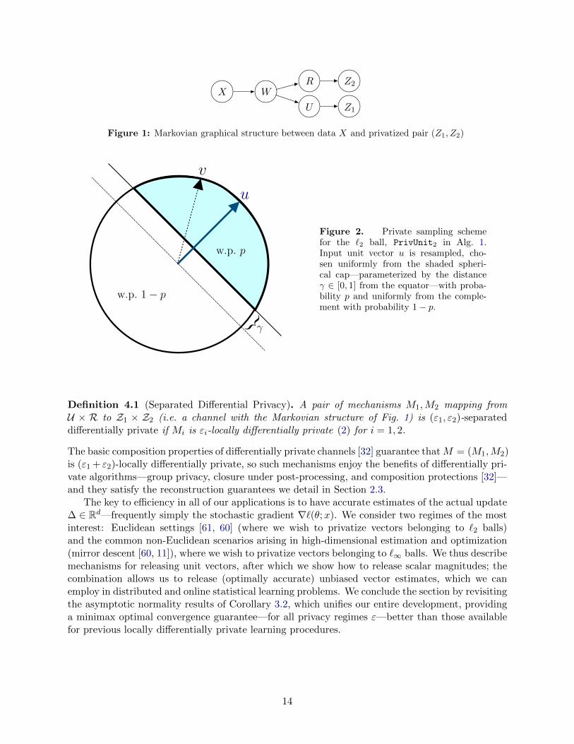
The main application of the privacy mechanisms we develop is to minimax rate-optimal private(distributed) statistical learning scenarios; accordingly, we now carefully consider mechanisms to usein the private updates (12). Motivated by the difficulties we outline in Section 1.2 for locally privatemodel fitting—in particular, that estimating the magnitude of a gradient or influence function ischallenging, and the scale of an update is essentially important—we consider mechanisms thattransmit information W ∈ Rd by privatizing a pair (U,R), where U = W/ ‖W‖2 is the directionand R = ‖W‖2 the magnitude, letting Z1 = M1(U) and Z2 = M2(R) be their privatized versions(see Fig. 1). We consider mechanisms satisfying the following definition.

13

X W

U

R

Z1

Z2

Figure 1: Markovian graphical structure between data X and privatized pair (Z1, Z2)

u

v

w.p. p

w.p. 1− p

γ

Figure 2. Private sampling schemefor the `2 ball, PrivUnit2 in Alg. 1.Input unit vector u is resampled, cho-sen uniformly from the shaded spheri-cal cap—parameterized by the distanceγ ∈ [0, 1] from the equator—with proba-bility p and uniformly from the comple-ment with probability 1− p.

Definition 4.1 (Separated Differential Privacy). A pair of mechanisms M1,M2 mapping fromU × R to Z1 × Z2 (i.e. a channel with the Markovian structure of Fig. 1) is (ε1, ε2)-separateddifferentially private if Mi is εi-locally differentially private (2) for i = 1, 2.

The basic composition properties of differentially private channels [32] guarantee thatM = (M1,M2)is (ε1 + ε2)-locally differentially private, so such mechanisms enjoy the benefits of differentially pri-vate algorithms—group privacy, closure under post-processing, and composition protections [32]—and they satisfy the reconstruction guarantees we detail in Section 2.3.

The key to efficiency in all of our applications is to have accurate estimates of the actual update∆ ∈ Rd—frequently simply the stochastic gradient ∇`(θ;x). We consider two regimes of the mostinterest: Euclidean settings [61, 60] (where we wish to privatize vectors belonging to `2 balls)and the common non-Euclidean scenarios arising in high-dimensional estimation and optimization(mirror descent [60, 11]), where we wish to privatize vectors belonging to `∞ balls. We thus describemechanisms for releasing unit vectors, after which we show how to release scalar magnitudes; thecombination allows us to release (optimally accurate) unbiased vector estimates, which we canemploy in distributed and online statistical learning problems. We conclude the section by revisitingthe asymptotic normality results of Corollary 3.2, which unifies our entire development, providinga minimax optimal convergence guarantee—for all privacy regimes ε—better than those availablefor previous locally differentially private learning procedures.

14

Algorithm 1 Privatized Unit Vector: PrivUnit2

Require: u ∈ Sd−1, γ ∈ [0, 1], p ≥ 12 .

Draw random vector V according to the distribution

V =

uniform on v ∈ Sd−1 | 〈v, u〉 ≥ γ with probability p

uniform on v ∈ Sd−1 | 〈v, u〉 < γ otherwise.(14)

Set α = d−12 , τ = 1+γ

2 , and

m =(1− γ2)α

2d−2(d− 1)

[p

B(α, α)−B(τ ;α, α)− 1− pB(τ ;α, α)

](15)

return Z = 1m · V

4.1 Privatizing unit `2 vectors with high accuracy

We begin with the Euclidean case, which arises in most classical applications of stochastic gradient-like methods [71, 61, 60]. In this case, we have a vector u ∈ Sd−1 (i.e. ‖u‖2 = 1), and we wish togenerate an ε-differentially private vector Z with the property that

E[Z | u] = u for all u ∈ Sd−1,

where the size ‖Z‖2 is as small as possible to maximize the efficiency in Corollary 3.2.We modify the sampling strategy of Duchi et al. [31] to develop an optimal mechanism. Given

a vector v ∈ Sd−1, we draw a vector V from a spherical cap v ∈ Sd−1 | 〈v, u〉 ≥ γ with someprobability p ≥ 1

2 or from its complement v ∈ Sd−1 | 〈v, u〉 < γ with probability 1 − p, whereγ ∈ [0, 1] and p are constants we shift to trade accuracy and privacy more precisely. In Figure 2,we give a visual representation of this mechanism, which we term PrivUnit2 (see Algorithm 1);in the next subsection we demonstrate the choices of γ and scaling factors to make the schemedifferentially private and unbiased. Given its inputs u, γ, and p, Algorithm 1 returns Z satisfyingE[Z | u] = u. We set the quantity m in Eq. (15) to guarantee this normalization, where

B(x;α, β) :=

∫ x

0tα−1(1− t)β−1dt where B(α, β) := B(1;α, β) =

Γ(α)Γ(β)

Γ(α+ β)

denotes the incomplete beta function. It is possible to sample from this distribution using in-verse CDF transformations and continued fraction approximations to the log incomplete beta func-tion [62].

In the remainder of this subsection, we describe the privacy preservation, bias, and varianceproperties of Algorithm 1.

4.1.1 Privacy analysis

Most importantly, Algorithm 1 protects privacy for appropriate choices of the spherical cap levelγ. Indeed, the next result shows that γε ≈

√ε/d is sufficient to guarantee ε-differential privacy.

Theorem 1. Let γ ∈ [0, 1] and p0 = eε01+eε0 . Then algorithm PrivUnit2(·, γ, p0) is (ε + ε0)-

differentially private whenever γ ≥ 0 is such that

ε ≥ log1 + γ ·

√2(d− 1)/π(

1− γ ·√

2(d− 1)/π)

+

, i.e. γ ≤ eε − 1

eε + 1

√π

2(d− 1), (16a)

15

or

ε ≥ 1

2log(d) + log 6− d− 1

2log(1− γ2) + log γ and γ ≥

√2

d. (16b)

Proof We again leverage the results in Appendix D. The random vector V ∈ Sd−1 in Alg. 1 hasdensity (conditional on u ∈ Sd−1)

p(v | u) ∝

p0/P(〈U, u〉 ≥ γ) if 〈v, u〉 ≥ γ(1− p0)/P(〈U, u〉 < γ) if 〈v, u〉 < γ.

We use that γ 7→ P(〈U, u〉 < γ) is increasing in γ to obtain (by definition of p0) that

p(v | u)

p(v | u′)≤ eε0 · P(〈U, u′〉 < γ)

P(〈U, u〉 ≥ γ), all u, u′ ∈ Sd−1. (17)

It is thus sufficient to prove that the last fraction has upper bound eε.We consider two cases in inequality (17). In the first, suppose that γ ≥

√2/d. Then Lemma D.1

impliesP(〈U, u′〉 < γ)

P(〈U, u〉 ≥ γ)≤ 6γ

√d

(1− γ2)d−12

,

which is bounded by eε when log 6 + 12 log d + log γ − d−1

2 log(1 − γ2) ≤ ε. In the second case,Lemma D.3 implies

P(〈U, u′〉 < γ)

P(〈U, u〉 ≥ γ)≤

1 + γ√

2(d− 1)/π

1− γ√

2(d− 1)/π,

which is bounded by eε if and only if γ ≤ eε−1eε+1

√π/(2(d− 1)).

4.1.2 Bias and variance

We now turn to optimality and error properties of Algorithm 1. Our first result is an lower boundon the `2-accuracy of any private mechanism, which follows from the paper of Duchi and Rogers[26].

Proposition 3. Assume that the mechanism M : Sd−1 → Rd is any of ε-differentially private,(ε, δ)-differentially private with δ ≤ 1

2 , or (ε∧ ε2, α)-Renyi differentially private for input x ∈ Sd−1,

all with ε ≤ d. Then for X uniformly distributed in ±1/√dd,

E[‖M(X)−X‖22] ≥ c · d

ε ∧ ε2∧ 1,

where c > 0 is a numerical constant. Moreover, if M is unbiased, then E[‖M(X)−X‖22] ≥ c dε∧ε2 .

Proof The first result is immediate by the result [26, Corollary 3]. For the unbiasedness lowerbound, note that if for a constant c0 < c we have E[‖M(X)−X‖22] ≤ c0

dε∧ε2 , then given a

sample X1, . . . , Xn ∈ ±1/√dd drawn i.i.d. from a population with mean θ = E[Xi], setting

Zi = M(Xi) we would have E[∥∥Zn − θ∥∥2

2] ≤ c0d

n(ε∧ε2). For small enough constant c0, this contra-

dicts [26, Cor. 3].

16

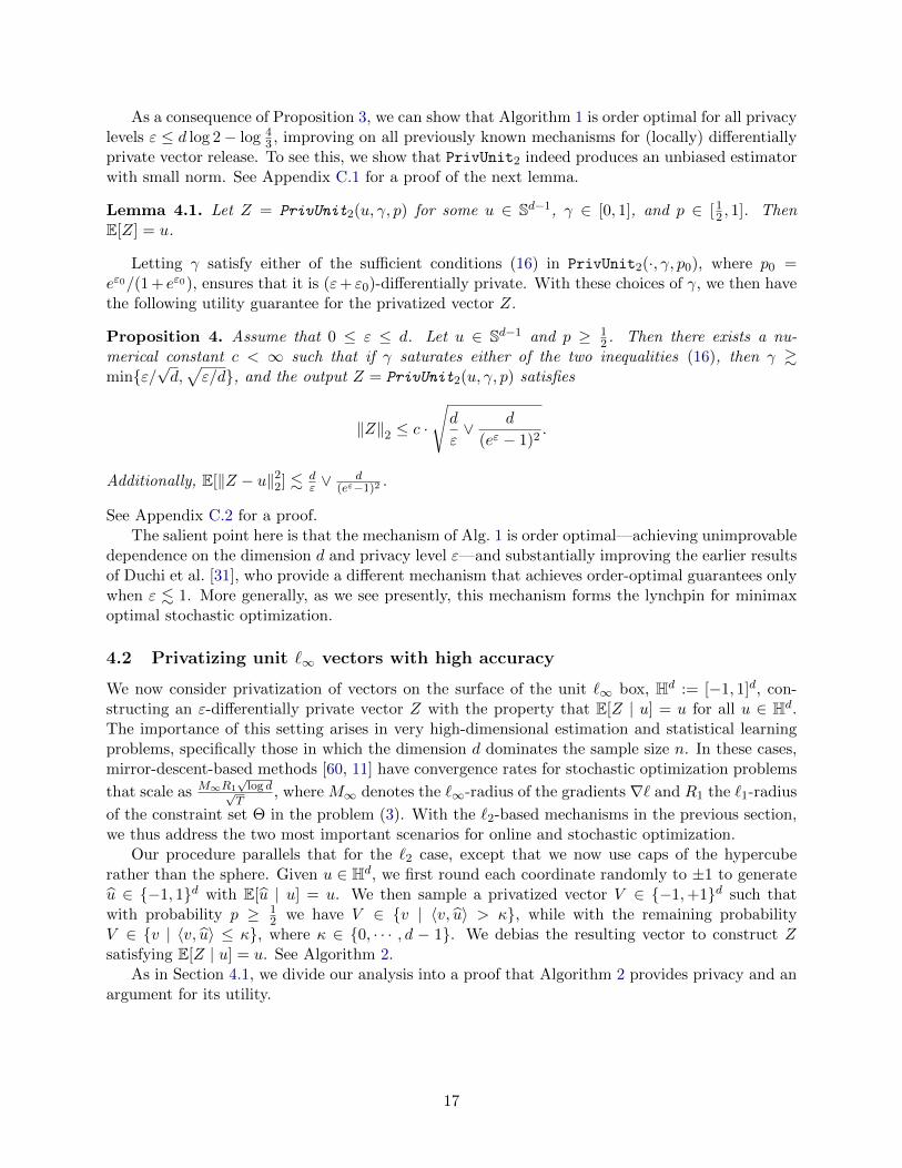
As a consequence of Proposition 3, we can show that Algorithm 1 is order optimal for all privacylevels ε ≤ d log 2− log 4

3 , improving on all previously known mechanisms for (locally) differentiallyprivate vector release. To see this, we show that PrivUnit2 indeed produces an unbiased estimatorwith small norm. See Appendix C.1 for a proof of the next lemma.

Lemma 4.1. Let Z = PrivUnit2(u, γ, p) for some u ∈ Sd−1, γ ∈ [0, 1], and p ∈ [12 , 1]. Then

E[Z] = u.

Letting γ satisfy either of the sufficient conditions (16) in PrivUnit2(·, γ, p0), where p0 =eε0/(1 + eε0), ensures that it is (ε+ ε0)-differentially private. With these choices of γ, we then havethe following utility guarantee for the privatized vector Z.

Proposition 4. Assume that 0 ≤ ε ≤ d. Let u ∈ Sd−1 and p ≥ 12 . Then there exists a nu-

merical constant c < ∞ such that if γ saturates either of the two inequalities (16), then γ &minε/

√d,√ε/d, and the output Z = PrivUnit2(u, γ, p) satisfies

‖Z‖2 ≤ c ·

√d

ε∨ d

(eε − 1)2.

Additionally, E[‖Z − u‖22] . dε ∨

d(eε−1)2

.

See Appendix C.2 for a proof.The salient point here is that the mechanism of Alg. 1 is order optimal—achieving unimprovable

dependence on the dimension d and privacy level ε—and substantially improving the earlier resultsof Duchi et al. [31], who provide a different mechanism that achieves order-optimal guarantees onlywhen ε . 1. More generally, as we see presently, this mechanism forms the lynchpin for minimaxoptimal stochastic optimization.

4.2 Privatizing unit `∞ vectors with high accuracy

We now consider privatization of vectors on the surface of the unit `∞ box, Hd := [−1, 1]d, con-structing an ε-differentially private vector Z with the property that E[Z | u] = u for all u ∈ Hd.The importance of this setting arises in very high-dimensional estimation and statistical learningproblems, specifically those in which the dimension d dominates the sample size n. In these cases,mirror-descent-based methods [60, 11] have convergence rates for stochastic optimization problems

that scale as M∞R1√

log d√T

, where M∞ denotes the `∞-radius of the gradients ∇` and R1 the `1-radius

of the constraint set Θ in the problem (3). With the `2-based mechanisms in the previous section,we thus address the two most important scenarios for online and stochastic optimization.

Our procedure parallels that for the `2 case, except that we now use caps of the hypercuberather than the sphere. Given u ∈ Hd, we first round each coordinate randomly to ±1 to generateu ∈ −1, 1d with E[u | u] = u. We then sample a privatized vector V ∈ −1,+1d such thatwith probability p ≥ 1

2 we have V ∈ v | 〈v, u〉 > κ, while with the remaining probabilityV ∈ v | 〈v, u〉 ≤ κ, where κ ∈ 0, · · · , d − 1. We debias the resulting vector to construct Zsatisfying E[Z | u] = u. See Algorithm 2.

As in Section 4.1, we divide our analysis into a proof that Algorithm 2 provides privacy and anargument for its utility.

17

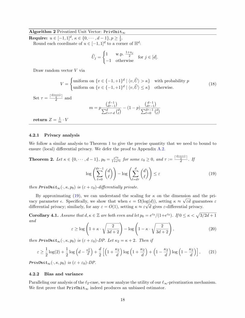
Algorithm 2 Privatized Unit Vector: PrivUnit∞

Require: u ∈ [−1, 1]d, κ ∈ 0, · · · , d− 1, p ≥ 12 .

Round each coordinate of u ∈ [−1, 1]d to a corner of Hd:

Uj =

1 w.p.

1+uj2

−1 otherwisefor j ∈ [d].

Draw random vector V via

V =

uniform on v ∈ −1,+1d | 〈v, U〉 > κ with probability p

uniform on v ∈ −1,+1d | 〈v, U〉 ≤ κ otherwise.(18)

Set τ =d d+κ+1

2e

d and

m = p

(d−1dτ−1

)∑d`=τ ·d

(d`

) − (1− p)(d−1dτ−1

)∑dτ−1`=0

(d`

)return Z = 1

m · V

4.2.1 Privacy analysis

We follow a similar analysis to Theorem 1 to give the precise quantity that we need to bound toensure (local) differential privacy. We defer the proof to Appendix A.2.

Theorem 2. Let κ ∈ 0, · · · , d− 1, p0 = eε01+eε0 for some ε0 ≥ 0, and τ :=

d d+κ+12e

d . If

log

(dτ−1∑`=0

(d

`

))− log

(d∑

`=dτ

(d

`

))≤ ε (19)

then PrivUnit∞(·, κ, p0) is (ε+ ε0)-differentially private.

By approximating (19), we can understand the scaling for κ on the dimension and the pri-vacy parameter ε. Specifically, we show that when ε = Ω(log(d)), setting κ ≈

√εd guarantees ε

differential privacy; similarly, for any ε = O(1), setting κ ≈ ε√d gives ε-differential privacy.

Corollary 4.1. Assume that d, κ ∈ Z are both even and let p0 = eε0/(1+eε0). If 0 ≤ κ <√

3/2d+ 1and

ε ≥ log

(1 + κ ·

√2

3d+ 2

)− log

(1− κ ·

√2

3d+ 2

), (20)

then PrivUnit∞(·, κ, p0) is (ε+ ε0)-DP. Let κ2 = κ+ 2. Then if

ε ≥ 1

2log(2) +

1

2log(d− κ22

d

)+d

2

[(1 +

κ2

d

)log(

1 +κ2

d

)+(

1− κ2

d

)log(

1− κ2

d

)], (21)

PrivUnit∞(·, κ, p0) is (ε+ ε0)-DP.

4.2.2 Bias and variance

Paralleling our analysis of the `2-case, we now analyze the utility of our `∞-privatization mechanism.We first prove that PrivUnit∞ indeed produces an unbiased estimator.

18

Lemma 4.2. Let Z = PrivUnit∞(u, κ) for some κ ∈ 0, · · · , d and u ∈ [−1, 1]. Then E[Z] = u.

See Appendix C.3 for a proof.The results of Duchi et al. [31] imply that for u ∈ −1, 1d the output Z = PrivUnit∞(u, κ =

0, p) has magnitude ‖Z‖∞ .√d p

1−p , which is√d e

ε+1eε−1 for p = eε/(1 + eε). We can, however,

provide stronger guarantees. Letting κ satisfy the sufficient condition (19) in PrivUnit∞(·, κ, p0)for p0 = eε0

eε0+1 ensures that Z is (ε+ ε0)-differentially private, and we have the utility bound

Proposition 5. Let u ∈ −1, 1d, p ≥ 12 , and Z = PrivUnit∞(u, κ, p). Then E[Z] = u, and there

exist numerical constants 0 < c0, c1 <∞ such that the following holds.

(i) Assume that ε ≥ log d. If κ saturates the bound (21), then κ ≥ c0

√εd and

‖Z‖∞ ≤ c1

√d

ε.

(ii) Assume that ε < log d. If κ saturates the bound (20), then κ ≥ c0 min√d, ε√d, and

‖Z‖∞ ≤ c1

√d

min1, ε.

See Appendix C.4 for a proof.Thus, comparing to the earlier guarantees of Duchi et al. [31], we see that this hypercube-cap-

based method we present in Algorithm 2 obtains no worse error in all cases of ε, and when ε ≥ log d,the dependence on ε is substantially better. An argument paralleling that for Proposition 3 showsthat the bounds on the `∞-norm of Z are unimprovable except for ε ∈ [1, log d]; we believe a slightlymore careful probabilistic argument should show that case (i) holds for ε ≥ 1.

4.3 Privatizing the magnitude

The final component of our mechanisms for releasing unbiased vectors is to privately release singlevalues r ∈ [0, rmax] for some rmax < ∞. The first (Sec. 4.3.1) provides a randomized-response-based mechanism achieving order optimal scaling for the mean-squared error E[(Z − r)2], which isr2

maxe−2ε/3 for ε ≥ 1 (see Corollary 8 in [38]). In the second (Sec. B.2), we provide a mechanism

that achieves better relative error guarantees—important for statistical applications in which wewish to adapt to the ease of a problem (recall the introduction), so that “easy” (small magnitudeupdate) examples indeed remain easy.

4.3.1 Absolute error

We first discuss a generalized randomized-response-based scheme for differentially private releaseof values r ∈ [0, rmax], where rmax is some a priori upper bound on r. We fix a value k ∈ N andthen follow a three-phase procedure: first, we randomly round r to an index value J taking valuesin 0, 1, 2, . . . , k so that

E[rmaxJ/k | r] = r and bkr/rmaxc ≤ J ≤ dkr/rmaxe .

In the second step, we employ randomized response [67] over k outcomes. The third step debi-ases this randomized quantity to obtain the estimator Z for r. We formalize the procedure inAlgorithm 3, ScalarDP.

Importantly, the mechanism ScalarDP is ε-differentially private, and we can control its accuracyvia the next lemma, whose proof we defer to Appendix B.1.

19

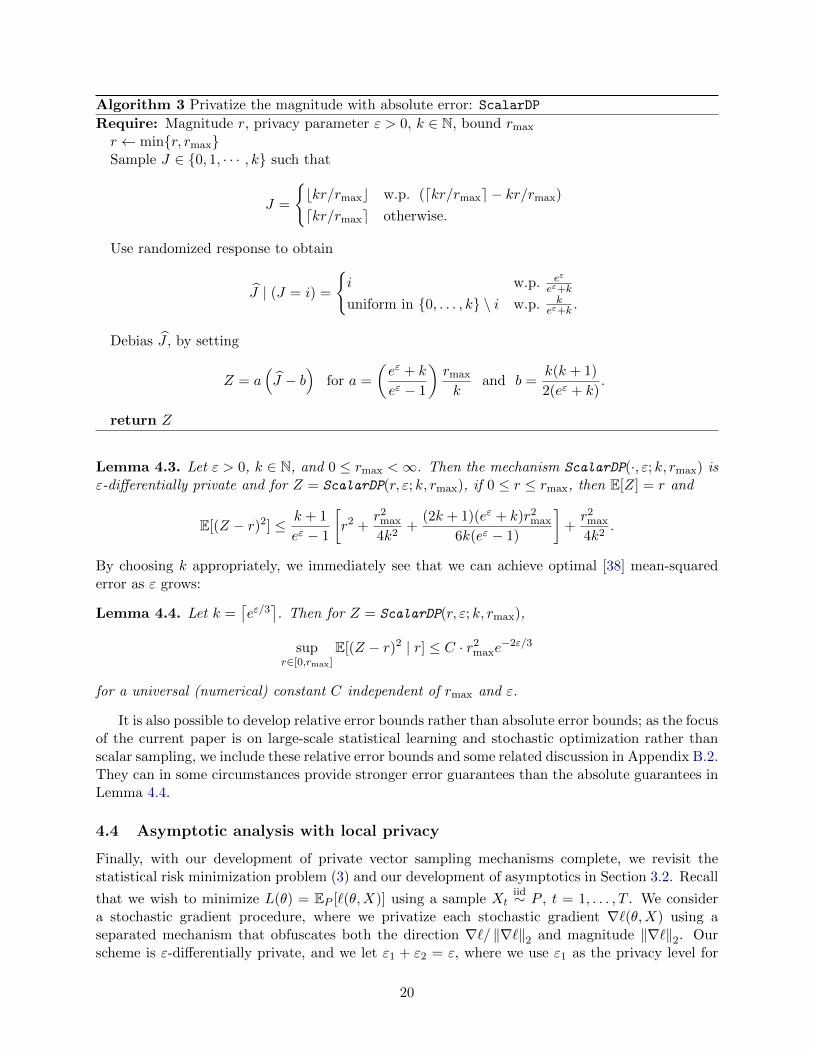
Algorithm 3 Privatize the magnitude with absolute error: ScalarDP

Require: Magnitude r, privacy parameter ε > 0, k ∈ N, bound rmax

r ← minr, rmaxSample J ∈ 0, 1, · · · , k such that

J =

bkr/rmaxc w.p. (dkr/rmaxe − kr/rmax)

dkr/rmaxe otherwise.

Use randomized response to obtain

J | (J = i) =

i w.p. eε

eε+k

uniform in 0, . . . , k \ i w.p. keε+k .

Debias J , by setting

Z = a(J − b

)for a =

(eε + k

eε − 1

)rmax

kand b =

k(k + 1)

2(eε + k).

return Z

Lemma 4.3. Let ε > 0, k ∈ N, and 0 ≤ rmax <∞. Then the mechanism ScalarDP(·, ε; k, rmax) isε-differentially private and for Z = ScalarDP(r, ε; k, rmax), if 0 ≤ r ≤ rmax, then E[Z] = r and

E[(Z − r)2] ≤ k + 1

eε − 1

[r2 +

r2max

4k2+

(2k + 1)(eε + k)r2max

6k(eε − 1)

]+r2

max

4k2.

By choosing k appropriately, we immediately see that we can achieve optimal [38] mean-squarederror as ε grows:

Lemma 4.4. Let k =⌈eε/3

⌉. Then for Z = ScalarDP(r, ε; k, rmax),

supr∈[0,rmax]

E[(Z − r)2 | r] ≤ C · r2maxe

−2ε/3

for a universal (numerical) constant C independent of rmax and ε.

It is also possible to develop relative error bounds rather than absolute error bounds; as the focusof the current paper is on large-scale statistical learning and stochastic optimization rather thanscalar sampling, we include these relative error bounds and some related discussion in Appendix B.2.They can in some circumstances provide stronger error guarantees than the absolute guarantees inLemma 4.4.

4.4 Asymptotic analysis with local privacy

Finally, with our development of private vector sampling mechanisms complete, we revisit thestatistical risk minimization problem (3) and our development of asymptotics in Section 3.2. Recall

that we wish to minimize L(θ) = EP [`(θ,X)] using a sample Xtiid∼ P , t = 1, . . . , T . We consider

a stochastic gradient procedure, where we privatize each stochastic gradient ∇`(θ,X) using aseparated mechanism that obfuscates both the direction ∇`/ ‖∇`‖2 and magnitude ‖∇`‖2. Ourscheme is ε-differentially private, and we let ε1 + ε2 = ε, where we use ε1 as the privacy level for

20

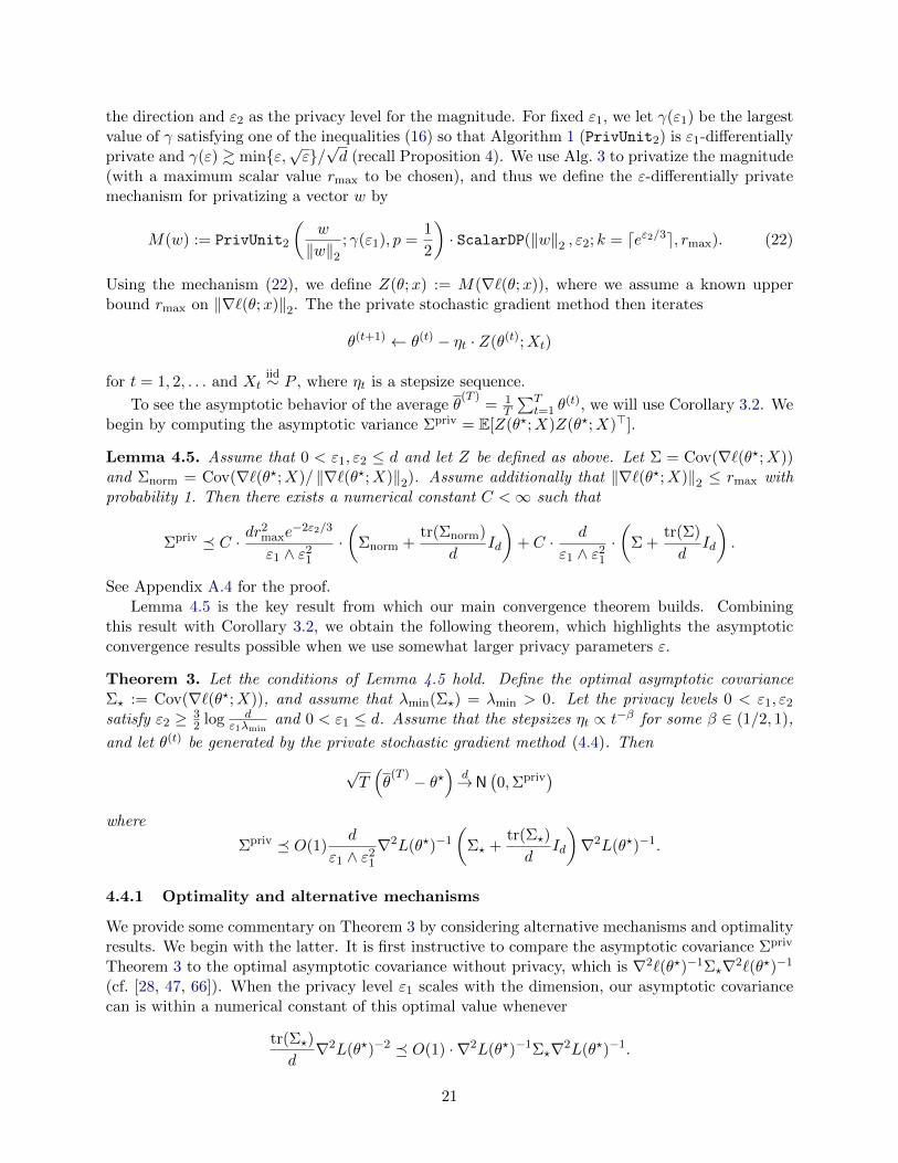
the direction and ε2 as the privacy level for the magnitude. For fixed ε1, we let γ(ε1) be the largestvalue of γ satisfying one of the inequalities (16) so that Algorithm 1 (PrivUnit2) is ε1-differentiallyprivate and γ(ε) & minε,

√ε/√d (recall Proposition 4). We use Alg. 3 to privatize the magnitude

(with a maximum scalar value rmax to be chosen), and thus we define the ε-differentially privatemechanism for privatizing a vector w by

M(w) := PrivUnit2

(w

‖w‖2; γ(ε1), p =

1

2

)· ScalarDP(‖w‖2 , ε2; k = deε2/3e, rmax). (22)

Using the mechanism (22), we define Z(θ;x) := M(∇`(θ;x)), where we assume a known upperbound rmax on ‖∇`(θ;x)‖2. The the private stochastic gradient method then iterates

θ(t+1) ← θ(t) − ηt · Z(θ(t);Xt)

for t = 1, 2, . . . and Xtiid∼ P , where ηt is a stepsize sequence.

To see the asymptotic behavior of the average θ(T )

= 1T

∑Tt=1 θ

(t), we will use Corollary 3.2. Webegin by computing the asymptotic variance Σpriv = E[Z(θ?;X)Z(θ?;X)>].

Lemma 4.5. Assume that 0 < ε1, ε2 ≤ d and let Z be defined as above. Let Σ = Cov(∇`(θ?;X))and Σnorm = Cov(∇`(θ?;X)/ ‖∇`(θ?;X)‖2). Assume additionally that ‖∇`(θ?;X)‖2 ≤ rmax withprobability 1. Then there exists a numerical constant C <∞ such that

Σpriv C · dr2maxe

−2ε2/3

ε1 ∧ ε21

·(

Σnorm +tr(Σnorm)

dId

)+ C · d

ε1 ∧ ε21

·(

Σ +tr(Σ)

dId

).

See Appendix A.4 for the proof.Lemma 4.5 is the key result from which our main convergence theorem builds. Combining

this result with Corollary 3.2, we obtain the following theorem, which highlights the asymptoticconvergence results possible when we use somewhat larger privacy parameters ε.

Theorem 3. Let the conditions of Lemma 4.5 hold. Define the optimal asymptotic covarianceΣ? := Cov(∇`(θ?;X)), and assume that λmin(Σ?) = λmin > 0. Let the privacy levels 0 < ε1, ε2

satisfy ε2 ≥ 32 log d

ε1λminand 0 < ε1 ≤ d. Assume that the stepsizes ηt ∝ t−β for some β ∈ (1/2, 1),

and let θ(t) be generated by the private stochastic gradient method (4.4). Then

√T(θ

(T ) − θ?)

d→N(0,Σpriv

)where

Σpriv O(1)d

ε1 ∧ ε21

∇2L(θ?)−1

(Σ? +

tr(Σ?)

dId

)∇2L(θ?)−1.

4.4.1 Optimality and alternative mechanisms

We provide some commentary on Theorem 3 by considering alternative mechanisms and optimalityresults. We begin with the latter. It is first instructive to compare the asymptotic covariance Σpriv

Theorem 3 to the optimal asymptotic covariance without privacy, which is ∇2`(θ?)−1Σ?∇2`(θ?)−1

(cf. [28, 47, 66]). When the privacy level ε1 scales with the dimension, our asymptotic covariancecan is within a numerical constant of this optimal value whenever

tr(Σ?)

d∇2L(θ?)−2 O(1) · ∇2L(θ?)−1Σ?∇2L(θ?)−1.

21

When Σ? is near identity, for example, this domination in the semidefinite order holds. We canof course never quite achieve optimal covariance, because the privacy channel forces some loss ofefficiency, but this loss of efficiency is now bounded. Even when ε1 is smaller, however, the resultsof Duchi and Rogers [26] imply that in a (local) minimax sense, there must be a multiplicationof at least O(1)d/minε, ε2 on the covariance ∇2`(θ?)−1Σ?∇2`(θ?)−1, which Theorem 3 exhibits.Thus, the mechanisms we have developed are indeed minimax rate optimal.

Let us consider alternative mechanisms, including related asymptotic results. First, considerDuchi et al.’s results generalized linear model estimation [31, Sec. 5.2]. In their case, in the identical

scenario, they achieve√T (θ

(T ) − θ?) d→N(0,Σmax) where the asymptotic variance Σmax satisfies

Σmax Ω(1)

(eε + 1

eε − 1

)2

∇2L(θ?)−1

(dΣ? + sup

x,θ‖∇`(θ;x)‖22 Id

)∇2L(θ?)−1.

There are two sources of looseness in this covariance, which is minimax optimal for some classesof problems [31]. First, supx,θ ‖∇`(θ;x)‖22 > tr(Σ?) = E[‖∇`(θ?;X)‖22]. Second, the error does not

decrease for ε > 1. Letting σ2ratio := supx,θ ‖∇`(θ;x)‖22 /E[‖∇`(θ?;X)‖22] > 1 denote the ratio of the

worst case norm to its expectation, which may be arbitrarily large, we have asymptotic `22-errorscaling as

tr(Σmax) &d

ε2 ∧ 1· tr(∇2L(θ?)−1Σ?∇2L(θ?)−1) +

σ2ratio

ε2 ∧ 1· tr(Σ?) tr(∇2L(θ?)−2)

tr(Σpriv) .d

ε2 ∧ ε· tr(∇2L(θ?)−1Σ?∇2L(θ?)−1) +

1

ε2 ∧ ε· tr(Σ?) tr(∇2L(θ?)−2).

The scaling of tr(Σpriv) reveals the importance of separately encoding the magnitude of ‖∇`(θ;X)‖2and its direction—we can be adaptive to the scale of Σ? rather than depending on the worst-casevalue supx,θ ‖∇`(θ;x)‖22.

Given the numerous relaxations of differential privacy [59, 33, 18] (recall Sec. 2.1, a naturalidea is to simply add noise satisfying one of these weaker definitions to the normalized vectoru = ∇`/ ‖∇`‖2 in our updates. Three considerations argue against this idea. First, these weak-enings can never actually protect against a reconstruction breach for all possible observations z(Definition 2.3)—they can only protect conditional on the observation z lying in some appropri-ately high probability set (cf. [9, Thm. 1]). Second, most standard mechanisms add more noisethan ours. Third, in a minimax sense—none of the relaxations of privacy even allow convergencerates faster than those achievable by pure ε-differentially private mechanisms [26].

Let us touch briefly on the second claim above about noise addition. In brief, our ε-differentiallyprivate mechanisms for privatizing a vector u with ‖u‖2 ≤ 1 in Sec. 4 release Z such that E[Z |u] = u and E[‖Z − u‖22 | u] . dmaxε−1, ε−2, which is unimprovable. In contrast, the Laplacemechanism and its `2 extensions [35] satisfy E[‖Z − u‖22 | u] & d2/ε2, which which yields worsedependence on the dimension d. Approximately differentially private schemes, which allow a δprobability of failure where δ is typically assumed sub-polynomial in n and d [34], allow mechanisms

such as Gaussian noise addition, where Z = u+W for W ∼ N(0,C log 1

δε2

) for C a numerical constant.

Evidently, these satisfy E[‖Z − u‖22 | u] & d log 1δ/ε

2, which again is looser than the mechanisms weprovide whenever ε . log 1

δ . Other relaxations—Renyi differential privacy [59] and concentrateddifferential privacy [33, 18]—similarly cannot yield improvements in a minimax sense [26], and theyprovide guarantees that the posterior beliefs of an adversary change little only on average.

22

5 Empirical Results

We present a series of empirical results in different settings, demonstrating the performance of our(minimax optimal) procedures for stochastic optimization in a variety of scenarios. In the settingswe consider—which simulate a large dataset distributed across multiple devices or units—the non-private alternative is to communicate and aggregate model updates without local or centralizedprivacy. We perform both simulated experiments (Sec. 5.1)—where we can more precisely showlosses due to privacy—and experiments on a large image classification task and language modeling.Because of the potential applications in modern practice, we use both classical (logistic regres-sion) models as well as modern deep network architectures [49], where we of course cannot proveconvergence but still guarantee privacy.

In each experiment, we use the `2-spherical cap sampling mechanisms of Alg. 1 in (ε1, ε2)-separated differentially private mechanisms (22). Letting γ(ε) be the largest value of γ satisfyingthe privacy condition (16) in our `2 mechanisms and p(ε) = eε

1+eε , for any vector w ∈ Rd, we use

M(w) := PrivUnit2

(w

‖w‖2; γ(0.99ε1), p(.01ε1)

)· ScalarDP

(‖w‖2 , ε2, k =

⌈eε2/3

⌉, rmax

). (23)

In our experiments, we set ε2 = 10, which is large enough (recall Theorem 3) so that its contributionto the final error is negligible relative to the sampling error in PrivUnit2 but of smaller order thanε1. In each experiment, we vary ε1, the dominant term in the asymptotic convergence of Theorem 3.

Our goal is to investigate whether private federated statistical learning—which includes sepa-rated differentially private mechanisms (providing local privacy protections against reconstruction)and central differential privacy—can perform nearly as well as models fit without privacy. Wepresent results both for models trained tabula rasa (from scratch, with random initialization) aswell as those pre-trained on other data, which is natural when we wish to update a model tobetter reflect a new population. Within each figure plotting results, we plot the accuracy of thecurrent model θk at iterate k versus the best accuracy achieved by a non-private model, providingerror bars over multiple trials. In short, we find the following: we can get to reasonably strongaccuracy—nearly comparable with non-private methods—for large values of local privacy parame-ter ε. However, with smaller values, even using (provably) optimal procedures can cause substantialperformance degradation.

Centralized aggregation In our large-scale real-data experiments, we include the centralizedprivacy protections by projecting (13) the updates onto an `2-ball of radius ρ, adding N(0, σ2I)noise with σ2 = Tq2ρ2/εα, where q is the fraction of users we subsample, T the total numberof updates, and εα the Renyi-privacy parameter we choose. In our experiments, we report theresulting centralized privacy levels for each experiment.

We make a concession to computational feasibility, slightly reducing the value σ that we actuallyuse in our experiments beyond the theoretical recommendations. In particular, we use batch sizem, corresponding to q = m/N , of at most 200 and test σ ∈ .001, .002, .005, .01, depending on ourexperiment, which of course requires either larger εα above or larger subsampling rate q than oureffective rate. As McMahan et al. [55] note, increasing this batch size has negligible effect on theaccuracy of the centralized model, so that we report results (following [55]) that use this inflatedbatch size estimate from a population of size N = 10,000,000.

23

5.1 Simulated logistic regression experiments

Our first collection of experiments focuses on a logistic regression experiment in which we canexactly evaluate population losses and errors in parameter recovery. We generate data pairs(Xi, Yi) ∈ Sd−1 × ±1 according to the logistic model

pθ(y | x) =1

1 + exp(−yθTx),

where the vectors Xi are i.i.d. uniform on the sphere Sd−1. In each experiment we choose the trueparameter θ? uniformly on τ ·Sd−1 so that τ > 0 reflects the signal-to-noise ratio in the problem. Inthis case, we perform the stochastic gradient method as in Sections 3.2 and 4.4 on the logistic loss`(θ; (x, y)) = log(1 + e−yx

T θ). For a given privacy level ε, in the update (22) we use the parameters

ε1 =13ε

16, ε2 =

ε

8, p =

eε/16

1 + eε/16,

that is, we privatize the direction g/ ‖g‖2 with ε1 = 1316ε-local privacy and flip probability p = eε/16

1+eε/16

and the magnitude ‖g‖2 using ε8 privacy.

Within each experiment, we draw a sample (Xi, Yi)iid∼ P of size N as above, and then perform

N stochastic gradient iterations using the mechanism (22). We choose stepsizes ηk = η0k−β for β =

.51, where the choice η0 =√ε/d, so that (for large magnitude noises) the stepsize is smaller—this

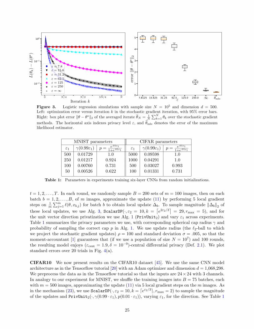
reflects the “optimal” stepsize tuning in standard stochastic gradient methods [60]. Letting L(θ) =E[`(θ;X,Y )] for the given distribution, we then evaluate L(θk)−L(θ?) and ‖θk − θ?‖2 over iterationsk, where θ? = argminθ L(θ). In Figure 3, we plot the results of experiments using dimension d = 500,sample size N = 105, and signal size τ = 4. (Other dimensions, sample sizes, and signal strengthsyield qualitatively similar results.) We perform 50 independent experiments, plotting aggregateresults. On the left plot, we plot the error of the private stochastic gradient methods, which—as we note earlier—are (minimax) optimal for this problem. We give 90% confidence intervalsacross all the experiments, and we see roughly the expected behavior: as the privacy parameter εincreases, performance approaches that of the non-private stochastic gradient estimator. The rightplot provides box plots of the error for the stochastic gradient methods as well as the non-privatemaximum likelihood estimator.

Perhaps the most salient point here is that, to maintain utility, we require non-trivially largeprivacy parameters for this (reasonably) high-dimensional problem; without ε ≥ d/8 the perfor-mance is essentially no better than that of a model using θ = 0, that is, random guessing. (Andalternative stepsize choices η0 do not help.)

5.2 Fitting deep models tabula rasa

We now present results on deep network model fitting for image classification tasks when we ini-tialize the model to have i.i.d. N(0, 1) parameters. Recall our mechanism (23), so that we allocateγ = γ(0.99ε1) for the spherical cap threshold and p = p(.01 · ε1) for the probability with whichwe choose a particular spherical cap in the randomization PrivUnit2(·, γ, p), which ensures ε1-differential privacy.

MNIST We begin with results on the MNIST handwritten digit recognition dataset [48]. We usethe default six-layer convolutional neural net (CNN) architecture of the TensorFlow tutorial [64]with default optimizer. The network contains d = 3, 274, 634 parameters. We proced in iterations

24

0 25 50 75 100 125 150 175 200

10 2

10 1

100

L(θ

k)−L

(θ?)

ε =∞ε = 250ε = 125ε = 62.5

ε = 31.2

ε = 15.6ε = 7.8

0 N/4 N/2 3N/4 N

Iteration k7.8125 15.625 31.25 62.5 125.0 250.0 inf inf

0

1

2

3

4

5

erro

r‖θ−θ?‖ 2

ε ∞ θmle

Figure 3. Logistic regression simulations with sample size N = 105 and dimension d = 500.Left: optimization error versus iteration k in the stochastic gradient iteration, with 95% error bars.

Right: box plot error ‖θ − θ?‖2 of the averaged iterate θN = 1N

∑Nk=1 θk over the stochastic gradient

methods. The horizontal axis indexes privacy level ε, and θmle denotes the error of the maximumlikelihood estimator.

MNIST parameters CIFAR parameters

ε1 γ(0.99ε1) p = e.01ε11+e.01ε1

ε1 γ(0.99ε1) p = e.01ε11+e.01ε1

500 0.01729 1.0 5000 0.09598 1.0250 0.01217 0.924 1000 0.04291 1.0100 0.00760 0.731 500 0.03027 0.99350 0.00526 0.622 100 0.01331 0.731

Table 1: Parameters in experiments training six-layer CNNs from random initializations.

t = 1, 2, . . . , T . In each round, we randomly sample B = 200 sets of m = 100 images, then on eachbatch b = 1, 2, . . . , B, of m images, approximate the update (11) by performing 5 local gradientsteps on 1

m

∑mj=1 `(θ, xb,j) for batch b to obtain local update ∆b. To sample magnitude ‖∆b‖2 of

these local updates, we use Alg. 3, ScalarDP(·, ε2 = 10, k =⌈e2ε2/3

⌉= 29, rmax = 5), and for

the unit vector direction privatization we use Alg. 1 (PrivUnit2) and vary ε1 across experiments.Table 1 summarizes the privacy parameters we use, with corresponding spherical cap radius γ andprobability of sampling the correct cap p in Alg. 1. We use update radius (the `2-ball to whichwe project the stochastic gradient updates) ρ = 100 and standard deviation σ = .005, so that themoment-accountant [1] guarantees that (if we use a population of size N = 107) and 100 rounds,the resulting model enjoys (εcent = 1.9, δ = 10−9)-central differential privacy (Def. 2.1). We plotstandard errors over 20 trials in Fig. 4(a).

CIFAR10 We now present results on the CIFAR10 dataset [45]. We use the same CNN modelarchitecture as in the Tensorflow tutorial [20] with an Adam optimizer and dimension d = 1,068,298.We preprocess the data as in the Tensorflow tutorial so that the inputs are 24×24 with 3 channels.In analogy to our experiment for MNIST, we shuffle the training images into B = 75 batches, eachwith m = 500 images, approximating the update (11) via 5 local gradient steps on the m images. Asin the mechanism (23), we use ScalarDP(·, ε2 = 10, k = deε2/3e, rmax = 2) to sample the magnitudeof the updates and PrivUnit2(·, γ(0.99 · ε1), p(0.01 · ε1)), varying ε1, for the direction. See Table 1

25

for the privacy parameters that we set in each experiment. We present the results in Figure 4(b)for mechanisms that satisfy (ε1, ε2 = 10)-separated DP where ε1 ∈ 100, 500, 1000, 5000. Thecorresponding `2-projection radius ρ = 30 and centralized noise addition of variance σ = .002guarantee, again via the moments-accountant [1], that with a “true” population size N = 107 andT = 200 rounds, the final model is (εcent = 1.76, δ = 10−9)-differneitally private. We plot thedifference in accuracies between federated learning and our private federated learning system withstandard errors over 20 trials.

0 20 40 60 80 100

Number of Rounds

10-2

10-1

Diffe

rence

in A

ccura

cy

MNIST Accuracy Plots for Private Federated Learning

Local eps1

50025010050

0 50 100 150 200

Number of Rounds

10-1

Diffe

rence

in A

ccura

cy

CIFAR10 Accuracy Plots for Private Federated Learning

Local eps1

50001000500100

(a) (b)

Figure 4. Accuracy plots for image classification comparing the private federated learning approach(indexed by privacy parameter ε1) with non-private model updates. Horizontal axis indexes numberof stochastic gradient updates, vertical the gap in test-set accuracy between the final non-privatemodel and the private model θk at the given round. (a) MNIST dataset. (b) CIFAR-10 dataset.

5.3 Pretrained models

Our final set of experiments investigates refitting a model on a new population. Given the largenumber of well-established and downloadable deep networks, we view this fine-tuning as a realisticuse case for private federated learning.

Image classification on Flickr over 100 classes We perform our first model tuning exper-iment on a pre-trained ResNet50v2 network [41] fit using ImageNet data [25], whose referenceimplementation is available at the website [50]. Beginning from the pre-fit model, we consider onlythe final (softmax) layer and final convolutional layer of the network to be modifiable, refitting themodel to perform 100-class multiclass classification on a subset of the Flickr corpus [65]. There ared = 1,255,524 parameters.

We construct a subsample for each of our experiments as follows. We choose 100 classes (uni-formly at random) and 2000 images from each class, yielding 2 · 105 images. We randomly permutethese into a 9:1 train/test split. In each iteration of the stochastic gradient method, we randomlychoose B = 100 sets of m = 128 images, performing an approximation to the proximal-pointupdate (11) using 15 gradient steps for each batch b = 1, 2, . . . , B. Again following the mecha-nism (23), for the magnitude of each update we use ScalarDP(·, ε2 = 10, k = deε2/3e, rmax = 10),while for the unit direction we use PrivUnit2(·, γ(0.99 · ε1), p(0.01 · ε1)) while varying ε1. Wepresent the results in Figure 5(a) for mechanisms that satisfy (ε1, ε2 = 10)-separated DP where

26

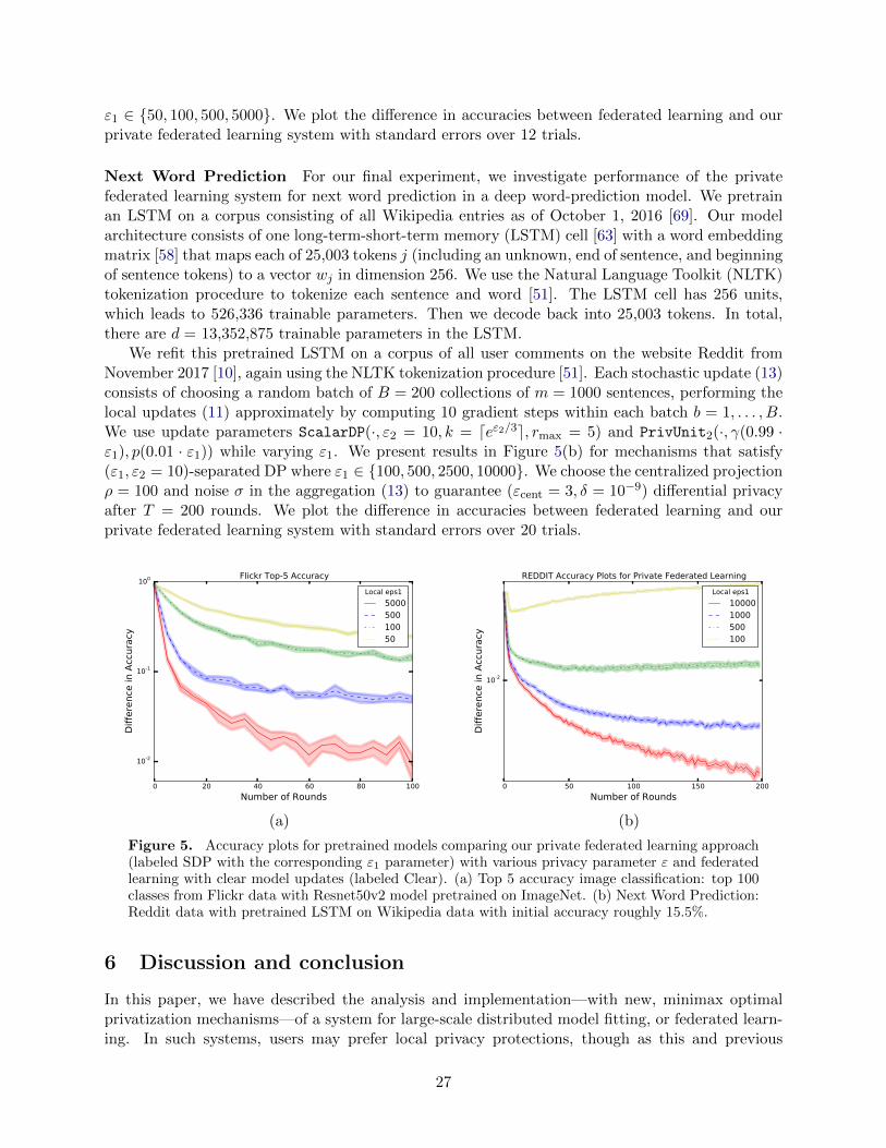
ε1 ∈ 50, 100, 500, 5000. We plot the difference in accuracies between federated learning and ourprivate federated learning system with standard errors over 12 trials.

Next Word Prediction For our final experiment, we investigate performance of the privatefederated learning system for next word prediction in a deep word-prediction model. We pretrainan LSTM on a corpus consisting of all Wikipedia entries as of October 1, 2016 [69]. Our modelarchitecture consists of one long-term-short-term memory (LSTM) cell [63] with a word embeddingmatrix [58] that maps each of 25,003 tokens j (including an unknown, end of sentence, and beginningof sentence tokens) to a vector wj in dimension 256. We use the Natural Language Toolkit (NLTK)tokenization procedure to tokenize each sentence and word [51]. The LSTM cell has 256 units,which leads to 526,336 trainable parameters. Then we decode back into 25,003 tokens. In total,there are d = 13,352,875 trainable parameters in the LSTM.

We refit this pretrained LSTM on a corpus of all user comments on the website Reddit fromNovember 2017 [10], again using the NLTK tokenization procedure [51]. Each stochastic update (13)consists of choosing a random batch of B = 200 collections of m = 1000 sentences, performing thelocal updates (11) approximately by computing 10 gradient steps within each batch b = 1, . . . , B.We use update parameters ScalarDP(·, ε2 = 10, k = deε2/3e, rmax = 5) and PrivUnit2(·, γ(0.99 ·ε1), p(0.01 · ε1)) while varying ε1. We present results in Figure 5(b) for mechanisms that satisfy(ε1, ε2 = 10)-separated DP where ε1 ∈ 100, 500, 2500, 10000. We choose the centralized projectionρ = 100 and noise σ in the aggregation (13) to guarantee (εcent = 3, δ = 10−9) differential privacyafter T = 200 rounds. We plot the difference in accuracies between federated learning and ourprivate federated learning system with standard errors over 20 trials.

0 20 40 60 80 100

Number of Rounds

10-2

10-1

100

Diffe

rence

in A

ccura

cy

Flickr Top-5 Accuracy

Local eps1

500050010050

0 50 100 150 200

Number of Rounds

10-2

Diffe

rence

in A

ccura

cy

REDDIT Accuracy Plots for Private Federated Learning

Local eps1

100001000500100

(a) (b)

Figure 5. Accuracy plots for pretrained models comparing our private federated learning approach(labeled SDP with the corresponding ε1 parameter) with various privacy parameter ε and federatedlearning with clear model updates (labeled Clear). (a) Top 5 accuracy image classification: top 100classes from Flickr data with Resnet50v2 model pretrained on ImageNet. (b) Next Word Prediction:Reddit data with pretrained LSTM on Wikipedia data with initial accuracy roughly 15.5%.

6 Discussion and conclusion

In this paper, we have described the analysis and implementation—with new, minimax optimalprivatization mechanisms—of a system for large-scale distributed model fitting, or federated learn-ing. In such systems, users may prefer local privacy protections, though as this and previous

27

work [31, 26] and make clear, providing small ε-local differential privacy makes model-fitting ex-tremely challenging. Thus, it is of substantial interest to understand what is possible in large εregimes, and the corresponding types of privacy such mechanisms provide; we have provided onesuch justification via prior beliefs and reconstruction probabilities from oblivious adversaries. Webelieve understanding appropriate privacy barriers, which provide different types of protections atdifferent levels, will be important for the practical adoption of private procedures, and we hopethat the current paper provides impetus in this direction.

7 Acknowledgements

We thank Aaron Roth for helpful discussions on earlier versions of this work. His comments helpedshape the direction of the paper.

28

References

[1] M. Abadi, A. Chu, I. Goodfellow, B. McMahan, I. Mironov, K. Talwar, and L. Zhang. Deeplearning with differential privacy. In 23rd ACM Conference on Computer and CommunicationsSecurity (ACM CCS), pages 308–318, 2016. URL https://arxiv.org/abs/1607.00133.

[2] J. Adelman-McCarthy et al. The sixth data release of the Sloan Digital Sky Survey. TheAstrophysical Journal Supplement Series, 175(2):297–313, 2008. doi: 10.1086/524984.

[3] Apple Differential Privacy Team. Learning with privacy at scale, 2017. Available at https:

//machinelearning.apple.com/2017/12/06/learning-with-privacy-at-scale.html.

[4] R. Ash. Information Theory. Dover Books on Advanced Mathematics. Dover Publications,1990. ISBN 9780486665214. URL https://books.google.com/books?id=yZ1JZA6Wo6YC.

[5] H. Asi and J. C. Duchi. The importance of better models in stochastic optimization.arXiv:1903.08619 [math.OC], 2019.

[6] H. Asi and J. C. Duchi. Stochastic (approximate) proximal point methods: Convergence,optimality, and adaptivity. SIAM Journal on Optimization, To Appear, 2019. URL https:

//arXiv.org/abs/1810.05633.

[7] P. Baldi, P. Sadowski, and D. Whiteson. Searching for exotic particles in high-energy physicswith deep learning. Nature Communications, 5, July 2014.

[8] K. Ball. An elementary introduction to modern convex geometry. In S. Levy, editor, Flavorsof Geometry, pages 1–58. MSRI Publications, 1997.

[9] R. F. Barber and J. C. Duchi. Privacy and statistical risk: Formalisms and minimax bounds.arXiv:1412.4451 [math.ST], 2014.

[10] J. Baumgartner. Reddit comments, 2017. URL http://files.pushshift.io/reddit/

comments/.

[11] A. Beck and M. Teboulle. Mirror descent and nonlinear projected subgradient methods forconvex optimization. Operations Research Letters, 31:167–175, 2003.

[12] D. P. Bertsekas. Incremental proximal methods for large scale convex optimization. Mathe-matical Programming, Series B, 129:163–195, 2011.

[13] D. P. Bertsekas and J. N. Tsitsiklis. Parallel and Distributed Computation: Numerical Methods.Prentice-Hall, Inc., 1989.

[14] K. Bonawitz, V. Ivanov, B. Kreuter, A. Marcedone, H. B. McMahan, S. Patel, D. Ram-age, A. Segal, and K. Seth. Practical secure aggregation for privacy-preserving machinelearning. In Proceedings of the 2017 ACM SIGSAC Conference on Computer and Com-munications Security, pages 1175–1191, New York, NY, USA, 2017. ACM. URL http:

//doi.acm.org/10.1145/3133956.3133982.

[15] L. Bottou and O. Bousquet. The tradeoffs of large scale learning. In Advances in NeuralInformation Processing Systems 20, 2007.

[16] S. Boucheron, G. Lugosi, and P. Massart. Concentration Inequalities: a Nonasymptotic Theoryof Independence. Oxford University Press, 2013.

29

[17] S. Boyd, N. Parikh, E. Chu, B. Peleato, and J. Eckstein. Distributed optimization and statis-tical learning via the alternating direction method of multipliers. Foundations and Trends inMachine Learning, 3(1), 2011.

[18] M. Bun and T. Steinke. Concentrated differential privacy: Simplifications, extensions, andlower bounds. In Theory of Cryptography Conference (TCC), pages 635–658, 2016.

[19] K. Chaudhuri, C. Monteleoni, and A. D. Sarwate. Differentially private empirical risk mini-mization. Journal of Machine Learning Research, 12:1069–1109, 2011.

[20] CifarTutorial. Advanced convolutional neural networks. https://www.tensorflow.org/

tutorials/images/deep_cnn, 2018.

[21] A. Clauset, C. Shalizi, and M. E. J. Newman. Power-law distributions in empirical data. SIAMReview, 51(4):661–703, 2009.

[22] A. N. Dajani, A. D. Lauger, P. E. Singer, D. Kifer, J. P. Reiter, A. Machanavajjhala, S. L.Garfinkel1, S. A. Dahl, M. Graham, V. Karwa, H. Kim, P. Leclerc, I. M. Schmutte, W. N.Sexton, L. Vilhuber, and J. M. Abowd. The modernization of statistical disclosure limitation atthe U.S. Census bureau. Available online at https://www2.census.gov/cac/sac/meetings/2017-09/statistical-disclosure-limitation.pdf, 2017.

[23] D. Davis and D. Drusvyatskiy. Stochastic model-based minimization of weakly convex func-tions. arXiv:1803.06523 [math.OC], 2018.

[24] J. Dean, G. S. Corrado, R. Monga, K. Chen, M. Devin, Q. V. Le, M. Z. Mao, M. Ranzato,A. Senior, P. Tucker, K. Yang, and A. Y. Ng. Large scale distributed deep networks. InAdvances in Neural Information Processing Systems 25, 2012.

[25] J. Deng, W. Dong, R. Socher, L. Li, K. Li, and L. Fei-Fei. ImageNet: a large-scale hierarchicalimage database. In Proceedings of the IEEE Conference on Computer Vision and PatternRecognition, 2009.

[26] J. C. Duchi and R. Rogers. Lower bounds for locally private estimation via communicationcomplexity. In Proceedings of the Thirty Second Annual Conference on Computational LearningTheory, 2019. URL https://arXiv.org/abs/1902.00582.

[27] J. C. Duchi and F. Ruan. The right complexity measure in locally private estimation: It isnot the Fisher information. arXiv:1806.05756 [stat.TH], 2018.

[28] J. C. Duchi and F. Ruan. Asymptotic optimality in stochastic optimization. Annals of Statis-tics, To Appear, 2019.

[29] J. C. Duchi, E. Hazan, and Y. Singer. Adaptive subgradient methods for online learning andstochastic optimization. Journal of Machine Learning Research, 12:2121–2159, 2011.

[30] J. C. Duchi, M. I. Jordan, and M. J. Wainwright. Local privacy and statistical minimax rates.In 54th Annual Symposium on Foundations of Computer Science, pages 429–438, 2013.

[31] J. C. Duchi, M. I. Jordan, and M. J. Wainwright. Minimax optimal procedures for locallyprivate estimation (with discussion). Journal of the American Statistical Association, 113(521):182–215, 2018.

30

[32] C. Dwork and A. Roth. The algorithmic foundations of differential privacy. Foundations andTrends in Theoretical Computer Science, 9(3 & 4):211–407, 2014. doi: 10.1561/0400000042.URL http://dx.doi.org/10.1561/0400000042.

[33] C. Dwork and G. Rothblum. Concentrated differential privacy. arXiv:1603.01887 [cs.DS],2016.

[34] C. Dwork, K. Kenthapadi, F. McSherry, I. Mironov, and M. Naor. Our data, ourselves: Privacyvia distributed noise generation. In Advances in Cryptology (EUROCRYPT 2006), 2006.

[35] C. Dwork, F. McSherry, K. Nissim, and A. Smith. Calibrating noise to sensitivity in privatedata analysis. In Proceedings of the Third Theory of Cryptography Conference, pages 265–284,2006.

[36] A. V. Evfimievski, J. Gehrke, and R. Srikant. Limiting privacy breaches in privacy preservingdata mining. In Proceedings of the Twenty-Second Symposium on Principles of DatabaseSystems, pages 211–222, 2003.

[37] M. Fredrikson, S. Jha, and T. Ristenpart. Model inversion attacks that exploit confidence infor-mation and basic countermeasures. In Proceedings of the 22Nd ACM SIGSAC Conference onComputer and Communications Security, pages 1322–1333, New York, NY, USA, 2015. ACM.doi: 10.1145/2810103.2813677. URL http://doi.acm.org/10.1145/2810103.2813677.

[38] Q. Geng and P. Viswanath. The optimal noise-adding mechanism in differential privacy. IEEETransactions on Information Theory, 62(2):925–951, 2016.

[39] M. Hardt and K. Talwar. On the geometry of differential privacy. In Proceedings of the Forty-Second Annual ACM Symposium on the Theory of Computing, pages 705–714, 2010. URLhttp://arxiv.org/abs/0907.3754.

[40] T. Hastie, R. Tibshirani, and J. Friedman. The Elements of Statistical Learning. Springer,second edition, 2009.

[41] K. He, X. Zhang, S. Ren, and J. Sun. Identity mappings in deep residual networks. In EuropeanConference on Computer Vision, pages 630–645, 2016. ISBN 978-3-319-46493-0.

[42] O. Kallenberg. Foundations of Modern Probability. Springer, 1997.

[43] N. Karampatziakis and J. Langford. Online importance weight aware updates. In Proceedingsof the 27th Conference on Uncertainty in Artificial Intelligence, 2011.

[44] N. D. Kazarinoff. Geometric Inequalities. Mathematical Association of America, 1961. doi:10.5948/UPO9780883859223.

[45] A. Krizhevsky. Learning multiple layers of features from tiny images. Technical report, Uni-versity of Toronto, 2009. URL https://www.cs.toronto.edu/~kriz/cifar.html.

[46] B. Kulis and P. Bartlett. Implicit online learning. In Proceedings of the 27th InternationalConference on Machine Learning, 2010.

[47] L. Le Cam and G. L. Yang. Asymptotics in Statistics: Some Basic Concepts. Springer, 2000.

[48] Y. LeCun, L. Bottou, Y. Bengio, and P. Haffner. Gradient-based learning applied to documentrecognition. In Advances in Neural Information Processing Systems 11, 1998.

31

[49] Y. LeCun, Y. Bengio, and G. Hinton. Deep learning. Nature, 521(7553):436–444, 2015.

[50] T. Lee. Tensornets. https://github.com/taehoonlee/tensornets, 2018.

[51] E. Loper and S. Bird. NLTK: The natural language toolkit. In Proceedings of the ACL-02Workshop on Effective Tools and Methodologies for Teaching Natural Language Processingand Computational Linguistics, pages 63–70, Stroudsburg, PA, USA, 2002. Association forComputational Linguistics. doi: 10.3115/1118108.1118117. URL https://doi.org/10.3115/

1118108.1118117.

[52] S. Mallat. A Wavelet Tour of Signal Processing: The Sparse Way (Third Edition). AcademicPress, 2008.

[53] H. B. McMahan, E. Moore, D. Ramage, S. Hampson, and B. A. y Arcas. Communication-efficient learning of deep networks from decentralized data. In Proceedings of the 20thInternational Conference on Artificial Intelligence and Statistics (AISTATS), 2017. URLhttp://arxiv.org/abs/1602.05629.

[54] H. B. McMahan, E. Moore, D. Ramage, S. Hampson, and B. A. y Arcas. Communication-efficient learning of deep networks from decentralized data. In Proceedings of the 20st Inter-national Conference on Artificial Intelligence and Statistics, 2017.

[55] H. B. McMahan, D. Ramage, K. Talwar, and L. Zhang. Learning differentially private languagemodels without losing accuracy. arXiv:1710.06963 [cs.LG], 2017. URL http://arxiv.org/

abs/1710.06963.

[56] L. Melis, C. Song, E. D. Cristofaro, and V. Shmatikov. Inference attacks against collaborativelearning. arXiv/1805.04049 [cs.CR], 2018. URL http://arxiv.org/abs/1805.04049.

[57] D. Micciancio and P. Voulgaris. Faster exponential time algorithms for the shortest vectorproblem. In Proceedings of the Twenty-First ACM-SIAM Symposium on Discrete Algorithms(SODA), 2010.

[58] T. Mikolov, I. Sutskever, K. Chen, G. Corrado, and J. Dean. Distributed representations ofwords and phrases and their compositionality. In Advances in Neural Information ProcessingSystems 26, 2013.

[59] I. Mironov. Renyi differential privacy. In 30th IEEE Computer Security Foundations Sympo-sium (CSF), pages 263–275, 2017.

[60] A. Nemirovski, A. Juditsky, G. Lan, and A. Shapiro. Robust stochastic approximation ap-proach to stochastic programming. SIAM Journal on Optimization, 19(4):1574–1609, 2009.

[61] B. T. Polyak and A. B. Juditsky. Acceleration of stochastic approximation by averaging. SIAMJournal on Control and Optimization, 30(4):838–855, 1992.

[62] W. H. Press, B. P. Flannery, S. A. Teukolsky, and W. T. Vetterling. Numerical Recipes in C:The Art of Scientific Computing, Second Edition. Cambridge University Press, 1992.

[63] J. Schmidhuber. Deep learning in neural networks: An overview. Neural networks, 61:85–117,2015.

[64] TensorFlowTutorial. Build a convolutional neural network using estimators. https://www.

tensorflow.org/tutorials/estimators/cnn, 2018.

32

[65] B. Thomee, D. Shamma, G. Friedland, B. Elizalde, K. Ni, D. Poland, D. Borth, and L. Li.Yahoo Flickr Creative Commons 100M: The new data in multimedia research. Communicationsof the ACM, 2(59):64–73, 2016.

[66] A. W. van der Vaart. Asymptotic Statistics. Cambridge Series in Statistical and ProbabilisticMathematics. Cambridge University Press, 1998. ISBN 0-521-49603-9.

[67] S. Warner. Randomized response: a survey technique for eliminating evasive answer bias.Journal of the American Statistical Association, 60(309):63–69, 1965.

[68] L. Wasserman and S. Zhou. A statistical framework for differential privacy. Journal of theAmerican Statistical Association, 105(489):375–389, 2010.

[69] Wikipedia. Wikimedia downloads, 2016. URL https://dumps.wikimedia.org. Accessed:10-01-2016.

[70] T. Zhang. Solving large scale linear prediction problems using stochastic gradient descentalgorithms. In Proceedings of the Twenty-First International Conference on Machine Learning,2004.

[71] M. Zinkevich. Online convex programming and generalized infinitesimal gradient ascent. InProceedings of the Twentieth International Conference on Machine Learning, 2003.

33

A Technical proofs

A.1 Proof of Lemma 2.3

We prove each result in turn. We begin with the precision bound. Fix p > 0, and assume thatpvT1 ≥ vTE[X]. Then using that Var(vj(Xj − E[Xj ])) ≤ vj

mj , and is 0 for j < m. By Bernstein’s

inequality, we then have

P(precision(v,X) ≥ p) = P(vT (X − E[X]) ≥ pvT1− vTE[X])

≤ exp

(− (pvT1− vTE[X])2

2∑

j>m vjVar(Xj) + 23(pvT1− vTE[X])

)

≤ exp

(−min

(pvT1− vTE[X])2

4∑

j>m vjVar(Xj),3

4(pvT1− vTE[X])

)(24)

For vT1 ≥ γm, assuming that p ≥ 1γ , we have

pvT1−vTE[X] ≥ pγm−γm∑j=1

E[Xj ] = pγm−m−γm∑

j=m+1

m

j≥ (pγ−1)m−m

∫ γm

m

1

tdt = (pγ−1−log γ)m.

For the first term in the exponent (24), the ratio again is maximized by v = (1γm,0d−γm), and wehave

d∑j=m+1

vjVar(Xj) ≤γm∑j>m

m

j≤ m

∫ γm

m

1

tdt = m log γ.

Substituting these bounds in Eq. (24), we have

P(precision(v,X) ≥ p) ≤ exp

(−min

(pγ − 1− log γ)2m

4 log γ,3

4(pγ − 1− log γ)m

).

For the recall bounds, we perform a similar derivation, assuming r ≤ 12 so that (1− r) ≥ r. We

temporarily assume (r1− v)TE[X] ≥ 0; we shall see that this holds. By Bernstein’s inequality, wehave

P(recall(v,X) ≥ r) = P(vTX ≥ r1TX) = P((v − r1)T (X − E[X]) ≥ (r1− v)TE[X])

≤ exp

(− ((r1− v)TE[X])2

2∑

j>m(r − vj)2Var(Xj) + 23(r1− v)TE[X]

)

≤ exp

(−min

((r1− v)TE[X])2

4∑

j>m(r − vj)2Var(Xj),3

4(r1− v)TE[X]

). (25)

We consider each term in the minimum (25) in turn. When∑

j vj ≤ γm, we have∑j>m

(r − vj)Var(Xj)2 ≤ m(1− r)2

∫ d

m

1

tdt = m(1− r)2 log

d

m,

while

(r1− v)TE[X] ≥ r1TE[X]−γm∑j=1

E[X] = rm+ rd∑

j=m+1

m

j−m−

γm∑j=m+1

E[Xj ]

≥ rm+ rm

∫ d

m+1

1

tdt−m−m

∫ γm

m

1

tdt = m

[r

(1 + log

d

m+ 1

)− 1− log γ

].

34

Substituting into inequality (25) gives the second result of the lemma.

A.2 Proof of Theorem 2

Let u ∈ −1,+1d and U ∼ Uni(−1,+1d). The vector V ∈ −1, 1d sampled as in (18), hasp.m.f.

p(v | u) ∝

1/P(〈U, u〉 > κ) if 〈v, u〉 > κ

1/P(〈U, u〉 < κ) if 〈v, u〉 ≤ κ.

The event that 〈U, u〉 = κ when d+κ+12 ∈ Z implies that U and umatch in exactly d+κ+1

2 coordinates;

the number of such matches is(

d(d+κ+1)/2

). Computing the binomial sum, we have

P(〈U, u〉 > κ) =1

2d

d∑`=d d+κ+1

2e

(d

`

)and P(〈U, u〉 ≤ κ) =

1

2d

d d+κ+12e−1∑

`=0

(d

`

).

As P(〈U, u〉 > κ) is decreasing in κ for any u, u′ ∈ −1,+1d and v ∈ −1, 1d we have

p(v | u)

p(v | u′)≤ p0

1− p0· P(〈U, u′〉 ≤ κ)

P(〈U, u〉 > κ)= eε0 ·

∑dτ−1`=0

(d`

)∑d`=dτ

(d`

) ,where τ = d(d+ κ)/2e. Bounding this by eε+ε0 gives the result.

A.3 Proof of Corollary 4.1

Using Theorem 2, we seek to bound the quantity (19) for various κ values. We first analyze thecase when κ ≤

√3/2d+ 1. We use the following claim to bound each term in the summation in

this case.

Claim A.1 (See Problem 1 in [44]). For even d ≥ 2, we have(d

d/2

)≤ 2d+1/2

√3d+ 2

Thus, when κ <√

3d+22 ,

log

(dτ−1∑`=0

(d

`

))− log

(d∑

`=dτ

(d

`

))= log

1/2 +1

2d·dτ−1∑`=d/2

(d

`

)− log

1/2− 1

2d

dτ−1∑`=d/2

(d

`

)≤ log

(1 + κ ·

(√2

3d+ 2

))− log

(1− κ ·

(√2

3d+ 2

)).

Hence, to ensure ε-differential privacy, it suffices to have

ε ≥ log

(1 + κ ·

√2

3d+ 2

)− log

(1− κ ·

√2

3d+ 2

),

so Eq. (20) follows.We now consider the case where ε = Ω(log(d)). We use the following claim.

35

Claim A.2 (Lemma 4.7.2 in [4]). Let Z ∼ Bin (d, 1/2). Then for 0 < λ < 1, we have

P(Z ≥ dλ) ≥ 1√8dλ(1− λ)

exp (−dDkl (λ||1/2))

We then use this to obtain the following bound:

log

(dτ−1∑`=0

(d

`

))− log

(d∑

`=dτ

(d

`

))≤ 1

2log (8dτ(1− τ)) + dDkl (τ ||1/2)

To ensure ε-differential privacy, it is thus sufficient, for τ :=d d+κ+1

2e

d , to have

ε ≥ 1

2log (8 · dτ(1− τ)) + d ·Dkl (τ ||1/2) ,

which implies the final claim of the corollary.

A.4 Proof of Lemma 4.5

For shorthand, define the radius R = ‖∇`(θ?;X)‖2, γ = γ(ε1), let U = ∇`(θ?;X)/ ‖∇`(θ?;X)‖2,and write

Z1 = PrivUnit2 (U ; γ, p = 1/2) Z2 = ScalarDP(R, ε2; k = deε2/3e, rmax)

so that Z = Z1Z2. Using that E[(Z2 −R)2 | R] ≤ O(r2maxe

−2ε2/3) by Lemma 4.4, we have

E[Z(θ?;X)Z(θ?;X)>] = E[E[Z1Z

>1 | U

]· E[Z2

2 | R]]

= E[E[Z1Z

>1 | U

]· E[(Z2 −R)2 | R

]]+ E

[R2 · E[Z1Z

>1 | U ]

] O(1)r2

maxe−2ε2/3 · E

[E[Z1Z

>1 | U

]]+ E

[R2 · E[Z1Z

>1 | U ]

]. (26)

We now focus on the term E[Z1Z>1 | U ]. Recall that V is uniform on v ∈ Sd−1 : 〈v, u〉 ≥ γ with

probability 12 and uniform on the complement v ∈ Sd−1 : 〈v, u〉 < γ otherwise (Eq. (14)). Then

for W ∼ Uni(Sd−1), we obtain E[V V > | u] = 12E[WW> | 〈W,u〉 ≥ γ] + 1

2E[WW> | 〈W,u〉 < γ],where

E[WW> | 〈W,u〉 ≥ γ] uu>+1− γ2

d− 1(Id−uu>) and E[WW> | 〈W,u〉 ≤ γ] uu>+

1

d(Id−uu>).

Both of these are in turn bounded by uu> + (1/d)Id. Using that the normalization m defined inEq. (15) satisfies m & minε1,

√ε1/√d by Proposition 4, we obtain

E[Z1Z>1 | U = u] 1

m2uu> +

1

dm2Id

d

ε1 ∧ ε21

uu> +1

ε1 ∧ ε21

Id.

Substituting this bound into our earlier inequality (26) and using that RU = ∇`(θ?;X), weobtain

E[Z(θ?;X)Z(θ?;X)>] O(1) · dr2maxe

−2ε2/3

ε1 ∧ ε21

· E[UU> + (1/d)Id]

+O(1) ·(

d

ε1 ∧ ε21

· E[∇`(θ?;X)∇`(θ?;X)>

]+

1

ε1 ∧ ε21

· E[‖∇`(θ?;X)‖22 Id

]).

Noting that tr(Cov(W )) = E[‖W‖22] for any random vector W gives the lemma.

36

B Scalar sampling

B.1 Proof of Lemma 4.3

That the mechanism is ε-differentially private is immediate as randomized response is ε-differentiallyprivate. To prove that Z is unbiased, we note that

E[J ] =kr

rmaxand E[Z | J ] =

rmax

kJ,

so that E[Z] = rmaxr E[J ] = r. To develop the bounds on the variance of Z, we use the standard

decomposition of variance into conditional variances, as

Var(Z) = E[(Z − r)2] = E [Var [Z | J ]] + Var [E [Z | J ]] = E[Var[Z | J ]] +r2

max

k2Var[J ].

We have Var[Z | J ] = a2 ·Var[J | J ]. Further, we have

E[J2 | J ] =

(eε − 1

eε + k

)· J2 +

(1

eε + k

)·k∑j=0

j2 and E[J | J ] =

(eε − 1

eε + k

)· J +

(1

eε + k

)·k∑j=0

j.

Combining the equalities and using that Var(Y ) = E[Y 2]− E[Y ]2, we have

Var[J | J ] =

(eε − 1

eε + k

)2

·((

eε + k

eε − 1− 1

)· J2 − k(k + 1)

eε − 1· J +

k(k + 1)(2k + 1)(eε + k)

6(eε − 1)2− k2(k + 1)2

4(eε − 1)2

).

We then have the conditional variance

Var[Z | J ] =r2

max

(eε − 1)2·(

(k + 1)(eε − 1)

k2· J2 − (k + 1)(eε − 1)

kJ +

(k + 1)(2k + 1)(eε + k)

6k− (k + 1)2

4

).

Now, note that J is a Bernoulli sample taking values in bkr/rmaxc , dkr/rmaxe. Thus, recallingthe notation Dec(t) = dte − t for the decimal part of a number, we have Var(J) = Dec( kr

rmax)(1 −

Dec( krrmax

)). Substituting all of these above and using that E[J2] = Var(J) +E[J ]2 = Var(J) + k2r2

r2max,

we obtain

Var(Z)

=r2

max

(eε − 1)2·(

(k + 1)(eε − 1)

k2

(k2r2

r2max

+ Dec(kr/rmax)(1− Dec(kr/rmax))

). . .

− (k + 1)(eε − 1)r

rmax+

(k + 1)(2k + 1)(eε + k)

6k− (k + 1)2

4

)+r2

max

k2Dec(kr/rmax)(1− Dec(kr/rmax))

≤ k + 1

eε − 1

[r2 +

r2max

4k2− rrmax +

(2k + 1)(eε + k)r2max

6k(eε − 1)− k + 1

4(eε − 1)

]+r2

max

4k2

where we have used that p(1−p) ≤ 14 for all p ∈ [0, 1]. Ignoring the negative terms gives the result.

37

B.2 Sampling scalars with relative error

As our discussion in the introductory Section 1.2 shows, to develop optimal learning procedures itis frequently important to know when the problem is easy—observations are low variance—and forthis, releasing scalars with relative error can be important. Consequently, we consider an alternativemechanism that first breaks the range [0, rmax] into intervals of increasing length based on a fixedaccuracy α > 0, k ∈ N, and ν > 1, where we define the intervals

E0 = [0, να], Ei = [νiα, νi+1α] for i = 1, . . . , k − 1. (27)

The resulting mechanism works as follows: we determine the interval that r belongs to, we randomlyround r to an endpoint of the interval (in an unbiased way), then use randomized response to obtaina differentially private quantity, which we then debias. We formalize the algorithm in Algorithm 4.

Algorithm 4 Privatize the magnitude with relative error: ScalarRelDP

Require: Magnitude r, privacy parameter ε > 0, integer k, accuracy α > 0, ν > 1, bound rmax.r ← minr, rmaxForm the intervals E0, E1, · · · , Ek−1 given in (27) and let i∗ be the index such that r ∈ Ei∗ .Sample J ∈ 0, 1, · · · , k such that

J =

0 w.p. να−r

να

1 w.p. rνα

if i∗ = 0 and J =

i∗ w.p. νi

∗+1α−rνi∗ (ν−1)α

i∗ + 1 w.p. r−νi∗ανi∗ (ν−1)α

if i∗ ≥ 1.

Use randomized response to obtain J

J | (J = i) =

i w.p. eε

eε+k

uniform in 0, . . . , k \ i w.p. keε+k .

Set J = ν J · 1J ≥ 1

Debias J , by setting

Z = a(J − b

)for a = α ·

(eε + k

eε − 1

)and b =

1

eε + k·k∑j=1

νj .

return Z

As in the absolute erorr case, we can provide an upper bound on the error of the mechanismScalarRelDP, though in this case—up to the small accuracy α—our error guarantee is relative.

Lemma B.1. Fix α > 0, k ∈ N, and ν > 1. Then Z = ScalarRelDP(·, ε; k, α, ν, rmax) is ε-differentially private and for r < rmax, we have E[Z | r] = r and

E[(Z − r)2 | r](r ∨ α)2

≤ (k + 1)

(eε − 1)ν2 +

(ν2k · (eε + k)

(eε − 1)2

)(1− ν−2k

1− ν−2

)+ (ν − 1)2.

See Appendix B.3 for a proof of Lemma B.1.

38

We perform a few calculations with Lemma B.1 when k ≤ eε. Let ν = 1 + ∆ for a ∆ ∈ (0, 1) tobe chosen, and note that the choice

k =

⌈log rmax

α

log ν

⌉≈

log rmaxα

∆

is the smallest value of k that gives νkα ≥ rmax. Let α = rmaxα0, so that ν2k ≈ 1α20. Hence, from

Lemma B.1 we have the truncated relative error bound

E[(Z − r)2 | r](r ∨ rmaxα0)2

.k

eε+

e−ε

α20 ·∆

+ ∆2 = e−ε(

log1

α0+

1

α20

)·(

1

∆

)+ ∆2 .

1

eεα20∆

+ ∆2.

We assume the relative accuracy threshold α/rmax = α0 & e−ε/2. Then setting ∆ = α−2/30 e−ε/3

givesE[(Z − r)2 | r](r ∨ rmaxα0)2

. α−4/30 e−2ε/3. (28)

Let us compare with Lemma 4.4, which yields

E[(Z − r)2 | r] = O(r2

maxe−2ε/3

).

The choice α0 = 1 in inequality (28) shows that the geometrically-binned mechanism can recoverthis bound. For r ≤ rmaxα0, the former inequality (28) is stronger; for example, the choice α0 =e−ε/4 yields that E[(Z−r)2 | r] = O(r2

maxe−5ε/6) for r ≤ rmaxe

−ε/4, and E[(Z−r)2 | r] = O(r2e−ε/3)otherwise.

B.3 Proof of Lemma B.1

To see that ScalarRelDP(·, k, α, ν; ε, rmax) is differentially private, we point out that randomizedresponse is ε-DP and then DP is closed under post-processing. To see that Z is unbiased, note that

E[J | J = i] =

(eε − 1

eε + k

)νi1 i ≥ 1+

1

eε + k

k∑j=1

νj ,

and thus for r ∈ Ei∗ ,

E[Z] = a · (E[J ]− b) = α ·(eε + k

eε − 1

)(eε − 1

eε + k

)E[νJ1 J ≥ 1] +

1

eε + k·k∑j=1

νj − 1

eε + k·k∑j=1

νj

= α · E

[νJ1 J ≥ 1

]= α ·

[1 i∗ = 0 ·

( r

αν

)· ν + 1 i∗ ≥ 1 ·

((νi∗+1α− r

νi∗(ν − 1)α

)· νi∗ +

(r − νi∗α

νi∗(ν − 1)α

)· νi∗+1

)]= 1 i∗ = 0 · r + 1 i∗ ≥ 1 · r = r

Consider the following mean squared error terms

E[(r − ανJ · 1 J ≥ 1)2 | r ∈ E0

]= r2

(1− r

αν

)+ (r − αν)2

( r

αν

)= r (αν − r) ≤ (να)2

And for i∗ ≥ 1

E[(r − ανJ · 1 J ≥ 1)2 | r ∈ Ei∗

]≤ (νi

∗+1α− νi∗α)2 = ν2i∗(νi∗ − 1)2α2.

39

We then bound the conditional expectation

Var(Z | J = i∗) = a2Var(J | J = i∗) = α2 ·(eε + k

eε − 1

)·Var(J | J = i∗),

Now we note that

Var(J | J = i∗) =

(eε − 1

eε + k

)· ν2i∗

1 i∗ ≥ 1+

(1

eε + k

)·k∑j=1

ν2j

−

(eε − 1

eε + k

)· νi∗1 i∗ ≥ 1+

(1

eε + k

)·k∑j=1

νj

2

≤(

(k + 1)(eε − 1)

(eε + k)2

)· ν2i∗

1 i∗ ≥ 1+

(1

eε + k

)· ν2k ·

k−1∑j=0

ν−2j

=

((k + 1)(eε − 1)

(eε + k)2

)· ν2i∗

1 i∗ ≥ 1+

(1

eε + k

)· ν2k ·

(1− ν−2k

1− ν−2

).

Now, if r ∈ Ei∗ , we have that νi∗α ≤ (r ∨ α) ≤ νi∗+1α, and thus

E[(Z − r)2]

(r ∨ α)2≤ α2

(r ∨ α)2·(eε + k

eε − 1

)2

·[

(k + 1)(eε − 1)

(eε + k)2ν2(i∗+1) +

ν2k

eε + k

(·1− ν

−2k

1− ν−2

)]+

α2

(r ∨ α)2· ν2i∗(ν − 1)2

≤ (k + 1)

(eε − 1)ν2 +

(ν2k · (eε + k)

(eε − 1)2

)(1− ν−2k

1− ν−2

)+ (ν − 1)2,

as desired.

C Proofs of utility in private sampling mechanisms

C.1 Proof of Lemma 4.1

Let u ∈ Sd−1 and U ∈ Sd−1 be a uniform random variable on the unit sphere. Then rotationalsymmetry implies that for some γ+ > 0 > γ−,

E[U | 〈U, u〉 ≥ γ] = γ+ · u and E[U | 〈U, u〉 < γ] = γ− · u,

and similarly, the random vector V in Algorithm 1 satisfies

E[V | u] = pE[U | 〈U, u〉 ≥ γ] + (1− p) · E[U | 〈U, u〉 < γ] = p(γ+ + γ−) · u.

By rotational symetry, we may assume u = e1, the first standard basis vector, without loss ofgenerality. We now compute the normalization constant. Letting U ∼ Uni(Sd−1) have coordinates

U1, . . . , Ud, we marginally Uidist= 2B − 1 where B ∼ Beta(d−1

2 , d−12 ). Now, we note that

γ+ = E[U1 | U1 ≥ γ] = E[2B − 1 | B ≥ 1+γ2 ] and γ− = E[U1 | U1 < γ] = E[2B − 1 | B < 1+γ

2 ]

40

and that if B ∼ Beta(α, β), then for 0 ≤ τ ≤ 1, we have

E[B | B ≥ τ ] =1

B(α, β) · P(B ≥ τ)

∫ 1

τxα(1− x)β−1dx =

B(α+ 1, β)−B(τ ;α+ 1, β)

B(α, β)−B(τ ;α, β)

and similarly E[B | B < τ ] = B(τ ;α+1,β)B(τ ;α,β) . Using that B(τ ;α+1, α) = B(α+1, α)[B(τ ;α,α)

B(α,α) −τα(1−τ)α

αB(α,α) ]

and B(α+1, α) = 12B(α, α), then substituting in our calculation for γ+ and γ−, we have for τ = 1+γ

2

and α = d−12 that

γ+ =1

α · 2d−1· (1− γ2)α

B(α, α)−B(τ ;α, α)and γ− =

−1

α2d−1· (1− γ2)α

B(τ ;α, α)

Consequently, E[V | u] = (pγ+ + (1 − p)γ−)u, and if Z = PrivUnit2(u, γ, p) we have E[Z] = u asdesired.

C.2 Proof of Proposition 4

Recall from the proof of Lemma 4.1 that Z = 1pγ++(1−p)γ−V , where E[U | 〈U, u〉 ≥ γ] = γ+ · u and

E[U | 〈U, u〉 < γ] = γ− · u for U = (U1, · · · , Ud) ∼ Uni(Sd−1), so that γ+ = E[U1 | U1 ≥ γ] ≥ γand, using E[|U1|] ≤ E[U2

1 ]1/2 ≤ 1/√d, we have γ− = E[U1 | U1 ≤ γ] ∈ [−E[|U1|], 0] ∈ [−1/

√d, 0].

Summarizing, we always have

γ ≤ γ+ ≤ 1, − 1√d≤ γ− ≤ 0, and |γ+| > |γ−|.

As a consequence, as the norm of V is 1 and ‖Z‖2 = 1/(pγ+ + (1 − p)γ−), which is decreasingto 1/γ+ as p ↑ 1, we always have ‖Z‖2 ≤

2γ++γ−

and we may assume w.l.o.g. that p = 12 in the

remainder of the derivation.Now, we consider three cases in the inequalities (16), deriving lower bounds on γ+ + γ− for

each.

1. First, assume 5 ≤ ε ≤ 2 log d. Let γ = γ0

√2/d for some γ0 ≥ 1. Then the choice γ0 = 1

guarantees that second inequality of (16b) holds, while we note that we must have γ20 ≤ d

d−1ε,

as otherwise d−12 log(1 − γ2

02d) ≤ −d−1

d γ20 < −ε, contradicting the inequality (16b). For γ0 ∈

[1,√

dd−1ε], we have log(1− γ2

02d) ≥ −8γ20

3d for sufficiently large d, and solving the first inequality

in Eq. (16b) we see it is sufficient that

4(d− 1)

3dγ2

0 ≤ ε− log2dε

d− 1− log 6 or γ2 ≤

6ε− 6 log 6− 3 log 2dεd−1

4(d− 1).

With this choice of γ, we obtain γ+ + γ− ≥ c√

dε for a numerical constant c.

2. For d ≥ ε ≥ 5, it is evident that (for some numerical constant c) the choice γ = c√ε/d satisfies

inequality (16b). Thus γ+ + γ− ≥ c√

dε .

3. Finally, we consider the last case that ε ≤ 5. In this case, the choice γ2 = π(eε−1)2/(2d(eε+1)2)satisfies inequality (16a). We need to control the difference γ+ + γ− = E[U1 | U1 ≥ γ] + E[U1 |

41

U1 ≤ γ]. In this case, let p+ = P(〈U, u〉 ≥ γ) and p− = P(〈U, u〉 < γ), so that Lemma D.3

implies that p+ ≤ 12 − e

−2γ√

d−12π and p− ≥ 1

2 + γ√

d−12π . Then

E[U1 | U1 ≥ γ] + E[U1 | U1 < γ] =1

p+E[U1 · 1 U1 ≥ γ] +

1

p−E[U1 · 1 U1 < γ]

=

(1

p+− 1

p−

)E[U1 · 1 U1 ≥ γ] ≥

(1− p+

p−

)E[U1 | U1 ≥ 0],

where the second equality follows from the fact that E[U1] = 0. Using that E[U1 | U1 ≥ 0] ≥cd−1/2 for a numerical constant c and

1− p+

p−≥

4e−2√

2(d−1)π

1 + 2e−2γ

√2(d−1)π

= Ω

(eε − 1

eε + 1

)

by our choice of γ, we obtain γ+ + γ− & (eε − 1)√d.

Combining the three cases above, we use that V in Alg. 1 has norm ‖V ‖2 = 1 and

‖Z‖2 ≤2

γ+ + γ−‖V ‖2 ≤ c

√d ·max ε−1, ε−2

to obtain the first result of the proposition.The final result of the proposition is immediate by the bound on ‖Z‖2.

C.3 Proof of Lemma 4.2

Without loss of generality, assume that u ∈ −1, 1d, as it is clear that E[U | u] = u in Algorithm 2.We now show that given u, E[V | u = u] = m · u. Consider U ∼ Uni(−1,+1d), in which case

E[V | u = u] = pE[U | 〈U, u〉 > κ] + (1− p)E[U | 〈U, u〉 ≤ κ].

For constants κ+, κ−, uniformity of U implies that

E[U | 〈U, u〉 > κ] = κ+ · u and E[U | 〈U, u〉 ≤ κ] = κ− · u.

By symmetry it is no loss of generality to assume that u = (1, 1, · · · , 1), so 〈U, u〉 =∑d

`=1 U`. Wethen have for τ = dd+κ+1

2 e/d that

E[U1 | 〈U, u〉 > κ] =1

2d · P(〈U, u〉 > κ)·

d∑`=dτ

((d− 1

`− 1

)−(d− 1

`

))=

(d−1dτ−1

)∑d`=dτ

(d`

) =: κ+

and

E[U1 | 〈U, u〉 ≤ κ] =1

2d · P(〈U, u〉 ≤ κ)·dτ−1∑`=0

((d− 1

`− 1

)−(d− 1

`

))=−(d−1dτ−1

)∑dτ−1`=0

(d`

) =: κ−.

Putting these together and setting m = pκ+ + (1− p)κ−, we have E[(1/m)V | u] = u.

42

C.4 Proof of Proposition 5

Using the notation of the proof of Lemma 4.2, the debiasing multiplierm satisfies 1/m = 1pκ++(1−p)κ− ≤

2κ++κ−

, as p ≥ 12 . Thus, we seek to lower bound κ+ +κ− by lower bounding κ+ and κ− individually.

We consider two cases: the case that ε ≥ log d and the case that ε < log d.

Case 1: when ε ≥ log d. We first focus on lower bounding

κ+ =

(d−1dτ−1

)∑d`=dτ

(d`

) = τ ·(ddτ

)∑d`=dτ

(d`

) = τ ·

(d∑

`=dτ

(d

dτ

)−1(d`

))−1

.

We argue that eventually the terms in the summation become small. For ` ≥ dτ defining

r :=dτ + 1

d− dτ≤ `+ 1

d− `=

(d`

)(d`+1

) implies

(d

`

)≥ r(

d

`+ 1

),

We then have

d∑`=dτ

(d

dτ

)−1(d`

)=

d−dτ∑i=0

(d

dτ

)−1( d

dτ + i

)≤

d−dτ∑i=0

(d

dτ

)−1( ddτ

)(1

r

)i=

d−dτ∑i=0

1

ri≤ 1

1− 1/r,

so that

κ+ ≥ 1− 1/r = 1− d− dτdτ + 1

=2dτ − d+ 1

dτ + 1=

2 · κ+2

d+κ+3 for odd d+ κ

2 · κ+3d+κ+4 for even d+ κ

≥ κ

d. (29)

We now lower bound κ−, where we use the fact that dτ−1 ≥ d−12 for κ ∈ 0, 1, · · · , d to obtain

κ− =−(d−1dτ−1

)∑τ ·d−1`=0

(d`

) = −τ(ddτ

)∑dτ−1`=0

(d`

) ≥ −τ ( ddτ)2d−1

.

Using Stirling’s approximation and that τ = dd+κ+12 e/d, we have(

d

dτ

)= C(κ, d)

√1

d· 2d · exp

(−κ

2

2d

),

where C(κ, d) is upper and lower bounded by positive universal constants. Hence, we have for aconstant c <∞,

κ− ≥ −c ·(

1√d· exp

(−κ2

2d

)). (30)

An inspection of the bound (21) shows that the choice κ = c√εd for some (sufficiently small)

constant c immediately satisfies the sufficient condition for Algorithm 2 to be private. Substitutingthis choice of κ into the lower bounds (29) and (30) gives that the normalizerm−1 ≤ 2

κ++κ−.√d/ε,

which is first result of Proposition 5.

43

Case 2: when ε < log d. In this case, we use the bound (20) to obtain the result. Let us firstchoose κ to saturate the bound (20), for which it suffices to choose κ = cmin

√d, ε√d for a

numerical constant c > 0. We assume for simplicity that d is even, as extending the argument issimply notational. Defining the shorthand sτ := 1

2d−1

∑dτ−1`=d/2

(d`

), we recall the definitions of κ+

and κ− to find

κ+ = τ ·(d

dτ

)· 1

1− sτand κ− = τ ·

(d

dτ

)· 1

1 + sτ.

Using the definition of the debiasing normalizer m = pκ+ + (1− p)κ− ≥ 12(κ+ + κ−), we obtain

m ≥ τ

2d

(d

dτ

)(1

1− sτ− 1

1 + sτ

)=

τ

2d

(d

dτ

)2sτ

1− s2τ

.

By definition of sτ , we have sτ ≥ dτ−d/22d−1

(ddτ

)≥ κ

2d

(ddτ

), so that

m & τκ

(2−d(d

dτ

))2

&1

dκ exp

(−κ

2

d

),

where the second inequality uses Stirling’s approximation. Our choice of κ = cmin√d, ε√d thus

yields m & 1√d

min1, ε, which gives the second result of Proposition 5.

D Uniform random variables and concentration

In this section, we collect a number of results on the concentration properties of variables uniformon the unit sphere Sd−1, which allow our analysis of the mechanism PrivUnit2 for privatizingvectors in the `2 ball in Algorithm 1. For a vector u ∈ Sd−1, that is, satisfying ‖u‖2 = 1, anda ∈ [0, 1] we define the spherical cap

C(a, u) :=v ∈ Sd−1 | 〈v, u〉 > a

.

There are a number of bounds on the probability that U ∈ C(a, u) for a fixed u ∈ Sd−1 whereU ∼ Uni(Sd−1), which the following lemma summarizes.

Lemma D.1. Let U be uniform on the unit sphere Sd−1 in Rd. Then for√

2/d ≤ a ≤ 1 andu ∈ Sd−1,

1

6a√d

(1− a2)d−12 ≤ P(U ∈ C(a, u)) ≤ 1

2a√d

(1− a2)d−12 . (31)

For all 0 ≤ a ≤ 1, we have

(1− a)

2d(1− a2)

d−12 ≤ P(U ∈ C(a, u)) (32)

and for a ∈ [0, 1/√

2],

P(U ∈ C(a, u)) ≤ (1− a2)d2 .

Proof The first result is [16, Exercise 7.9]. The lower bound of the second is due to [57, Lemma4.1], while the third inequality follows for all a ∈ [0, 1/

√2] by [8, Proof of Lemma 2.2].

We also require a slightly different lemma for small values of the threshold a in Lemma D.1.

44

Lemma D.2. Let γ ≥ 0 and U be uniform on Sd−1. Then

γ

√d− 1

2πexp

(− 1

4d− 4− 1

)1

γ ≤

√2/(d− 3)

≤ P(〈U, u〉 ∈ [0, γ]) ≤ γ

√d− 1

2π

Proof For any fixed unit vector u ∈ Sd−1 and U ∼ Uni(Sd−1), we have that marginally 〈U, u〉 ∼2B − 1 for B ∼ Beta(d−1

2 , d−12 ). Thus we have

P(〈U, u〉 ∈ [0, γ]) = P(

1

2≤ B ≤ 1 + γ

2

)We will upper and lower bound the last probability above. Letting α = d−1

2 for shorthand, we have

P(

1

2≤ B ≤ 1 + γ

2

)=

Γ(2α)

Γ(α)2

∫ 1+γ2

12

tα−1(1− t)α−1dt

(i)=

Γ(2α)

2Γ(α)2

∫ γ

0

(1 + u

2

)α−1(1− u2

)α−1

du =Γ(2α)

22α−1Γ(α)2

∫ γ

0(1− u2)α−1du,

where equality (i) is the change of variables u = 2t − 1. Using Stirling’s approximation, we havethat

log Γ(2α)− 2 log Γ(α) = (2α− 1) log 2 +1

2log

α

π+ err(α),

where err(α) ∈ [− 18α ,−

18α+1 ]. When γ ≤

√1/(α− 1), we have

∫ γ

0(1− u2)α−1du ≥

∫ γ

0

1−

(√1

α− 1

)2α−1

du ≥ γe−1

Otherwise, if γ >√

1/(α− 1) we have the trivial bound∫ γ

0 (1 − u2)α−1du ≥ 0. Furthermore, forγ ≥ 0 we have

∫ γ0 (1− u2)α−1du ≤ γ. Putting this all together, we have

exp

(− 1

8α

)·(√

α

π

)·(γe−1

)· 1γ ≤ (α− 1)−

12

≤ exp(err(α))

√α

π

∫ γ

0(1− u2)α−1du = P

(1

2≤ B ≤ 1 + γ

2

)≤ γ

√α

π.

Substituting α 7→ d−12 yields the desired upper and lower bounds on P(〈U, u〉 ∈ [0, γ]).

As a consequence of Lemma D.2, we have the following result.

Lemma D.3. Let γ ∈ [0,√

2/(d− 3)] and U be uniform on Sd−1. Then

1

2− γ√d− 1

2π≤ P(U ∈ C(γ, u)) ≤ 1

2− γ√d− 1

2πe−

4d−34d−4 .

Proof We have

P (U ∈ C(γ, u)) = 1− P (〈U, u〉 < γ) = 1/2− P (〈U, u〉 ∈ [0, γ)) .

We then use Lemma D.2

45