Property price separation between

land and building components

by

Ünsal Özdilek

Paper submitted for publication in the Journal of Real Estate Research

Contact address:

Ünsal Özdilek, Business School, Department of Strategy, social and

environmental responsibilities, University of Quebec, Montreal City,

Canada, H3C 3P8

Phone: (519) 987-3000, extension: 4436

Fax : (514) 987-0422

Email : ozdilek.unsal@uqam.ca

Property price separation between

land and building components

Abstract

Observed sales prices are direct references for the market value of properties, but they do not

provide information about the separate values of land and building. There are different theories

and methods, each one being limited in practice. This paper presents the troublesome issue of

price separation and proposes a practical alternative, using detailed data from Montreal

(Canada). The empirical results support the separability thesis in practice for the cases of

residential properties.

Keywords: property price; land; building; improvements; value apportionment;

separate evaluation

1

1. Introduction

Land valuation is quite easy when there are sufficient comparable vacant lands being sold on the

market. This is hardly the situation nowadays in most built-up cities where more than ever before the

land market is progressively disappearing, and land value is becoming an ever more elusive concept.

What is negotiated and appears commonly in the deed of sales is a total price paid for the entire

property. There is no direct indication of the separate components of prices for the land and the

improvements.

Land value has traditionally been explained in terms of classical production rent, neoclassical utility,

location rent, social dynamics and political decisions. Each of these concepts contributes of course to

the explanations, but they are in general theoretical and restricted with various hypotheses. Even in the

recent literature, based on the empirical modeling culture and data, the price apportionment between

land and building components has always had a low priority. The analysis of the dialectic between the

two components is missing; they are analysed in isolation or mixed. However, there are some confusing

echoes from classical fields of revenue imputation and property tax impacts.

Arguments on the inseparability thesis have been presented by Ely (1922), Russell (1945), Ratcliff

(1950), Fisher (1958) and Dorau and Hinman (1969), and are restated in some contemporary views

(Mills, 1998; Robinson, 1999; Fischel, 2000; Kitchen, 2003; Hendricks, 2005). The consensus is that

apportionment is not practicable (and is useless) because land and improvements are merged together

like an “omelette” to form a new joint product. In contrast, several early authors proposed or defended

separation (Smith, 1886; George, 1898; Marshall, 1922; Brueckner, 1986; Oates and Schwab, 1997).

While explanations from both sides are essentially theoretical, some responses might come from the

practice of appraisal using the three classical methods of price, cost and income. The similar theoretical

debates can be confusing, but in practice what matters are total value estimations, notably for taxation

purposes (Rice, 1997; Andelson, 2000).

The issue of apportionment thus remains troublesome. Despite the “silence” surrounding

improvements and the general omission in practice, land value continues to exist and shape the

dynamics of real estate markets. It even progressively catches up with the value of the improvements,

sometimes going much further. While there is no empirical evidence of this, many practical situations

require separate estimations, for example city and capital gains taxation, tax incidences (Gloudemans,

2

2001), challenges by contributors in courts (Keligan, 1994), applicability of the cost method for

improvements only (Appraisal Institute, 2001), decisions about depreciation, amortization,

renovations, and demolitions (Arnott and Petrova, 2002), management of insurances and mortgages

(Guofang et al., 2003), to measure the speculative effects on land (agricultural) and its products (Stokes

and Cox, 2014), sound land use policies and practices (Dancaescu, 2000) or addressing land value

maps (Ohno, 1985).

The issue of apportionment is relevant everywhere and concerns all types of properties, especially

housing in urbanized areas for which land market is scarce and classic methods are ineffective. This

paper focuses on the issue of apportionment of price between the land and the improvements for

residential properties in the context of mass valuations. It develops an original alternative of price

separation using the framework of measure theory and a large database from the city of Montreal

(Canada).

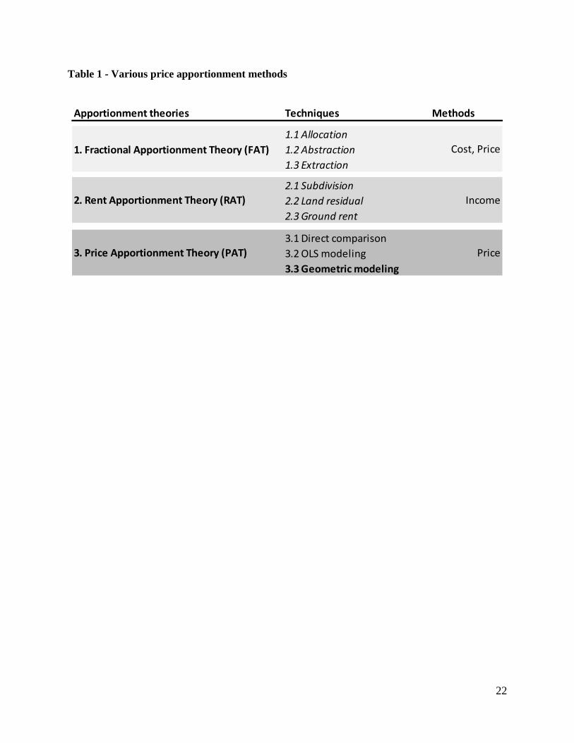
2. Price apportionment methods

There are three possible price apportionment theories supporting different techniques and methods in

practice, listed in Table 1 and discussed in Özdilek (2012), in which we add the last alternative of

geometric modeling elaborated in this paper. In the list, the approach that is closest to our proposed

method is the OLS model which allows one to decompose the total price of properties between their

multiple utility generating parameters (Lancaster, 1966; Rosen, 1974; Sirmans et al., 2005).

There have been a few attempts to estimate land value parameters, by considering data only on vacant

land sales (Clapp, 1990; Isakson, 1997; Colwell, 1998). Shi (2014) more recently elaborated an

approach to improve the “net rate” factor, classically used in the conceptual framework of separation

by the extraction technique. Other studies used total prices, separated between land and improvements

(Guerin, 2000; Gloudemans, 2002; and Plassmann and Tideman, 2003). These studies relax key

contingencies of the separation issue in the hedonic framework by having recourse to both improved

and unimproved land sales in the same model, meaning that separation is not possible otherwise.

Özdilek (2011) presents a separation technique from a hedonic approach, providing conceptual as well

as empirical details of price separation.

<Insert Table 1>

3

Classical methods in both FAT and RAT theories are approximate and do not provide reliable results.

They are essentially subjective as they precede ad hoc almost by a rule of thumb and some simple

assumptions (Oates and Schwab, 1997; Mills, 1998; Anas, 2003). The parametric approach, which

essentially refers to the hedonic modeling tradition through multiple linear or nonlinear regression

analysis (Breiman, 2001), proposes an interesting solution. However, it is limited to the independence

hypothesis between the parameters and the accuracy of their isolated contributions. If there are errors

of estimation per utility attribute of the properties, the sum of their individual errors might be

significant in separate estimations. There is also the difficulty of separating the constant and the error

terms of the models which increase, especially when the price determinant parameters are missing.

In the geometric approach presented in this paper, we assume that when lands are identical or very

similar (given their proper multiple attributes), if there is a variation in total prices, it comes mainly

from the building component. Inversely, the same hypothesis applies when the building components

are identical. Based on this fundamental proposition, we maintain the simplicity and the objectivity of

the sales comparison method in a straightforward manner, using a large set of observations. Our

nonparametric approach achieves separation by starting from the attributes of the properties as given

and then observing price differentials, whereas in the OLS technique, the process begins by breaking

down the total prices between the parameters and then assembling their “estimated” utility

contributions in the land and building values.

Both approaches are exposed, though in different ways, to the problem of interactions (for parameter

variations in space, see Pavlov, 2000), because we cannot presume they will be entirely eliminated for

the simple reason that lands and buildings go together. But, if we create similar conditions starting

from the separate parameters and then use the price differentials, as in our approach, we can at least

hope to keep any possible interactions constant. For example, if the lands are identical or very similar

(same usage, sector, size, physical form, proximity to various location points such as a park or a

school), then the interactions with the building components will be the same (though not eliminated).

In those circumstances, the differences in price originate from the building. The same reasoning applies

when the building parameters are constant (e.g., living area, number of stories, external recovery or

types of floors) and the lands are different. Even the competition in the market encourages an optimal

level of combinations; there are however some cases of over and under improvements, against the

principle of the Highest and Best Use (HBU).

4

Another concern is that the sum of the values of the land and the building might be less than the total

value of the property. From the modern view of finance, total value might include an Option value for

unimproved lands (Quigg, 1993) as well as an option to redevelop improved lands (Williams, 1991;

Clapp et al., 2012) or to renovate (Plaut and Plaut, 2010). This would be the case with another intricate

agent known as Business value which originates from entrepreneurial efforts and managerial abilities

(Martin and Nafe, 1996). There is a debate on that issue, but Miller et al. (1995) and Rabiansky (1996)

consider them as being parts of the land and the building. In our approach, the values of these types of

agents are held constant in time and space by creating similar conditions for the utility expressions of

the improvements. Also, the redevelopment or the renovation options are explainable in the model by

the inclusion of the various parameters of age, condition, sector, and location quality. The particular

and inverse relation progressing in time between the land and building components deserves more

attention in a context of uncertainty, using the option value framework. In fact, as land usually gains

value over time while buildings always depreciate, it would be interesting to know when to consider

redevelopment, for example by taking into account the imbalances in their ratios and the evolution of

the construction costs.

On a technical note, there is an unexplained residual of value which is usually specified under the form

of an error term in the equations of statistical approaches. Our geometrical approach, which is different

in nature, does not use such a statistical measure, but it indirectly has the conditions of the error

“sharing” following the parameters initially gathered in one or the other component. Using a high

number of comparables with the appropriate parameters which should help to reduce the significance

of that term (which also has treatments in the field of spatial autocorrelation – Anselin, 1995).

3. Main concepts of the model

The approach we have developed for separate price estimation uses the properties of measure theory

in a geometric space representation (Halmos, 1974; Royden, 1988). Although the comparison between

parametric OLS models and the nonparametric separation method proposed here may seem irrelevant

because the underlying theory is different, we can argue that our model would perform well since the

final price is estimated from observations that are very similar to the subject’s land and building

components.

5

The main concepts and the mathematical expressions of that model are presented in the following

sections in relation to total and separate price predictions. Some details of the equations and the

practical algorithms are reported in the Appendix.

3.1 Prediction of the total price

We define a utility space 𝑼 as a (locally Euclidean) subspace of the standard Euclidean space 𝑅𝑁 for

a finite or infinite 𝑁 > 0. As a subspace, 𝑼 has a number of observable coordinate functions 𝑢𝑖. We

suppose that 𝑖 belongs to a finite set {1, … ,𝑀}, and that 𝑢𝑖’s are global coordinates and express

characteristics of properties (i.e., size, number of rooms, presence of a swimming pool, proximity to

urban parks, etc.). The utility space 𝑼 has to be appropriate with a sufficient number 𝑀 of observable

functions 𝑢𝑖 allowing one to distinguish prices 𝑃𝑖, 𝑃𝑗 for different properties 𝑖, 𝑗.

Property price 𝑷 is a nonnegative function 𝑃:𝑼 → 𝑅+ and it is a measure on utility space 𝑼, so that

(𝑼,𝑷) is a measure of space in a proper sense. 𝑷(𝐴) expresses the total price of properties, identified

with all points of the set 𝐴 ⊂ 𝑼.

The density (Radon-Nikodym derivative) 𝑑𝑷

𝑑𝜇𝐿, where 𝑑𝜇𝐿: = 𝑑𝑢1 ∧ ⋯∧ 𝑑𝑢𝑀 is the Lebesgue measure

on 𝑼, exists and is the price 𝑃(𝑢) of property 𝑢 ∈ 𝑼. Measure 𝜇𝐿 is sigma-finite as the measure on a

subspace of Euclidean space 𝑅𝑁. 𝑷 << 𝜇𝐿 is absolutely continuous since 𝜇𝐿(𝐴) = 0 ⇒ 𝑷(𝐴) = 0 and

the derivative exists. The meaning of 𝑷 here is the point price 𝑃(𝑢), 𝑢 ∈ 𝑼.

All events (observable cases) happen in the measure space (𝑼,𝑷), i.e., the class of observable

properties 𝐾 = 𝐾sold ∪ 𝐾unsold belong to the space (𝑼,𝑷) (where the set 𝐾sold denotes given statistical

data). The set 𝐾sold, similarly to the space (𝑼, 𝑷), carries (at least) two different measures: 𝑷sold, which

assigns the sum of prices of all properties located in a subset of 𝐾sold, and 𝜇count, which counts points

of a subset of 𝐾sold. These measures are in a very similar relation to the measures 𝑷 and 𝜇𝐿 on 𝑼.

The density (Radon-Nikodym derivative) 𝑑𝑷𝑠𝑜𝑙𝑑

𝑑𝜇𝑠𝑜𝑙𝑑 exists and is the price 𝑃(𝑢) of property 𝑢 ∈ 𝐾sold. At

this point we have two models: continuous (𝑼,𝑷, 𝜇𝐿) and discrete (𝐾sold, 𝑷sold, 𝜇count). Radon-

Nikodym derivative 𝑑𝑷𝑠𝑜𝑙𝑑

𝑑𝜇𝑠𝑜𝑙𝑑 of the discrete space (𝐾sold, 𝑷sold, 𝜇count) “converges” to Radon-Nikodym

6

derivative 𝑑𝑷

𝑑𝜇𝐿 of the continuous space (𝑼,𝑷, 𝜇𝐿) when cardinality (or the data size) of the set 𝐾sold is

sufficiently high. To make this important observation clear the idea of convergence needs to be

explained. It can be understood as just an enhancement of the continuous model with new points or in

a proper way as a pointwise convergence in the space of Lebesgue measurable functions on 𝑼 when

the statistical data are linearly interpolated on small pieces over all 𝑼. Let 𝔉 be any filter of Lebesgue

measurable sets on 𝑼 converging to a point 𝑢 ∈ 𝑼. Then

𝑃(𝑢) = lim𝔉→𝑢

𝑷(𝑂)

𝜇𝐿(𝑂)≈ lim

𝔉sold→𝑢

𝑃𝑠𝑜𝑙𝑑(𝑂𝑠𝑜𝑙𝑑)

𝜇𝑐𝑜𝑢𝑛𝑡(𝑂𝑠𝑜𝑙𝑑), (1)

𝑂 ∈ 𝔉, 𝔉sold = 𝔉 ∩ 𝐾sold, 𝑂sold = 𝑂 ∩ 𝐾sold ∈ 𝔉sold.

The expression in (1) shows that when the number of observed cases 𝑂sold (or the references in the

discrete data) increases, this better reflects the behavior of the market. This idea of convergence in a

continuous case supports our main proposition and method of separation with a discrete case. It holds

a simple, but subtle point exemplified in Table 3. Using average point prices for the land and the

building requires reliable “average total prices” from the filtered similar properties to the subject.

For example, when land characteristics are kept similar (or constant) in the data, the number of

references should increase sufficiently to provide a reliable average total price. This total price

approaches the real total price in the market by increasing the number of comparables, thereby

justifying the use of the “average price of the buildings” (or that of the lands). Following that objective,

we cannot be very rigid in creating high similarity which will end up with an insufficient number of

comparables (and consequently move away from the real average prices). So, the precision depends

mainly on the size of the data: the more it increases the more reliable are the estimates, as might be the

case in the context of mass appraisals.

A practical realization of the algorithm for estimating the total price of a property is presented in the

Appendix. This algorithm assigns to an unknown point the average value of the price of the known

ones most similar to it. In this small neighbourhood the algorithm acts linearly (assigning the

barycentre of the points around). So, the approximation is piecewise linear (the actual price function

looks as if it is covered by small scales on the small pieces where the data 𝐾sold are missed). As the

number of the data increases these scales become smaller and smaller, coinciding with pieces of tangent

hyperplanes.

7

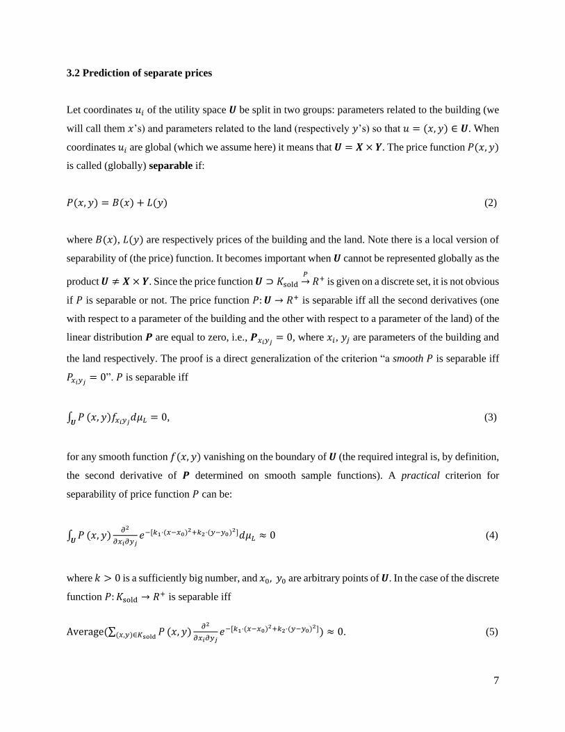
3.2 Prediction of separate prices

Let coordinates 𝑢𝑖 of the utility space 𝑼 be split in two groups: parameters related to the building (we

will call them 𝑥’s) and parameters related to the land (respectively 𝑦’s) so that 𝑢 = (𝑥, 𝑦) ∈ 𝑼. When

coordinates 𝑢𝑖 are global (which we assume here) it means that 𝑼 = 𝑿 × 𝒀. The price function 𝑃(𝑥, 𝑦)

is called (globally) separable if:

𝑃(𝑥, 𝑦) = 𝐵(𝑥) + 𝐿(𝑦) (2)

where 𝐵(𝑥), 𝐿(𝑦) are respectively prices of the building and the land. Note there is a local version of

separability of (the price) function. It becomes important when 𝑼 cannot be represented globally as the

product 𝑼 ≠ 𝑿 × 𝒀. Since the price function 𝑼 ⊃ 𝐾sold

𝑃→ 𝑅+ is given on a discrete set, it is not obvious

if 𝑃 is separable or not. The price function 𝑃:𝑼 → 𝑅+ is separable iff all the second derivatives (one

with respect to a parameter of the building and the other with respect to a parameter of the land) of the

linear distribution 𝑷 are equal to zero, i.e., 𝑷𝑥𝑖𝑦𝑗= 0, where 𝑥𝑖, 𝑦𝑗 are parameters of the building and

the land respectively. The proof is a direct generalization of the criterion “a smooth 𝑃 is separable iff

𝑃𝑥𝑖𝑦𝑗= 0”. 𝑃 is separable iff

∫ 𝑃𝑼

(𝑥, 𝑦)𝑓𝑥𝑖𝑦𝑗𝑑𝜇𝐿 = 0, (3)

for any smooth function 𝑓(𝑥, 𝑦) vanishing on the boundary of 𝑼 (the required integral is, by definition,

the second derivative of 𝑷 determined on smooth sample functions). A practical criterion for

separability of price function 𝑃 can be:

∫ 𝑃𝑼

(𝑥, 𝑦)𝜕2

𝜕𝑥𝑖𝜕𝑦𝑗𝑒−[𝑘1⋅(𝑥−𝑥0)

2+𝑘2⋅(𝑦−𝑦0)2]𝑑𝜇𝐿 ≈ 0 (4)

where 𝑘 > 0 is a sufficiently big number, and 𝑥0, 𝑦0 are arbitrary points of 𝑼. In the case of the discrete

function 𝑃:𝐾sold → 𝑅+ is separable iff

Average(∑ 𝑃(𝑥,𝑦)∈𝐾sold(𝑥, 𝑦)

𝜕2

𝜕𝑥𝑖𝜕𝑦𝑗𝑒−[𝑘1⋅(𝑥−𝑥0)

2+𝑘2⋅(𝑦−𝑦0)2]) ≈ 0. (5)

8

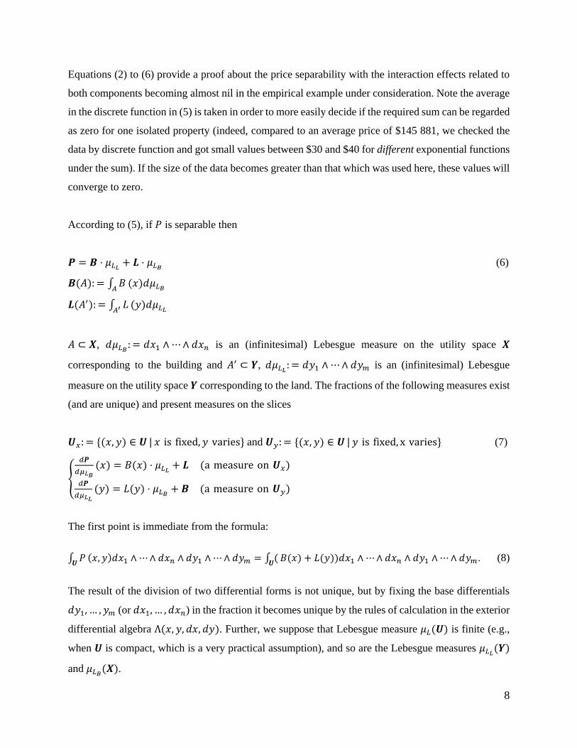
Equations (2) to (6) provide a proof about the price separability with the interaction effects related to

both components becoming almost nil in the empirical example under consideration. Note the average

in the discrete function in (5) is taken in order to more easily decide if the required sum can be regarded

as zero for one isolated property (indeed, compared to an average price of $145 881, we checked the

data by discrete function and got small values between $30 and $40 for different exponential functions

under the sum). If the size of the data becomes greater than that which was used here, these values will

converge to zero.

According to (5), if 𝑃 is separable then

𝑷 = 𝑩 ⋅ 𝜇𝐿𝐿+ 𝑳 ⋅ 𝜇𝐿𝐵

(6)

𝑩(𝐴):= ∫ 𝐵𝐴

(𝑥)𝑑𝜇𝐿𝐵

𝑳(𝐴′): = ∫ 𝐿𝐴′ (𝑦)𝑑𝜇𝐿𝐿

𝐴 ⊂ 𝑿, 𝑑𝜇𝐿𝐵: = 𝑑𝑥1 ∧ ⋯∧ 𝑑𝑥𝑛 is an (infinitesimal) Lebesgue measure on the utility space 𝑿

corresponding to the building and 𝐴′ ⊂ 𝒀, 𝑑𝜇𝐿𝐿: = 𝑑𝑦1 ∧ ⋯∧ 𝑑𝑦𝑚 is an (infinitesimal) Lebesgue

measure on the utility space 𝒀 corresponding to the land. The fractions of the following measures exist

(and are unique) and present measures on the slices

𝑼𝑥: = {(𝑥, 𝑦) ∈ 𝑼 | 𝑥 is fixed, 𝑦 varies} and 𝑼𝑦: = {(𝑥, 𝑦) ∈ 𝑼 | 𝑦 is fixed, x varies} (7)

{

𝑑𝑷

𝑑𝜇𝐿𝐵

(𝑥) = 𝐵(𝑥) ⋅ 𝜇𝐿𝐿+ 𝑳 (a measure on 𝑼𝑥)

𝑑𝑷

𝑑𝜇𝐿𝐿

(𝑦) = 𝐿(𝑦) ⋅ 𝜇𝐿𝐵+ 𝑩 (a measure on 𝑼𝑦)

The first point is immediate from the formula:

∫ 𝑃𝑼

(𝑥, 𝑦)𝑑𝑥1 ∧ ⋯∧ 𝑑𝑥𝑛 ∧ 𝑑𝑦1 ∧ ⋯∧ 𝑑𝑦𝑚 = ∫ (𝑼

𝐵(𝑥) + 𝐿(𝑦))𝑑𝑥1 ∧ ⋯∧ 𝑑𝑥𝑛 ∧ 𝑑𝑦1 ∧ ⋯∧ 𝑑𝑦𝑚. (8)

The result of the division of two differential forms is not unique, but by fixing the base differentials

𝑑𝑦1, … , 𝑦𝑚 (or 𝑑𝑥1, … , 𝑑𝑥𝑛) in the fraction it becomes unique by the rules of calculation in the exterior

differential algebra Λ(𝑥, 𝑦, 𝑑𝑥, 𝑑𝑦). Further, we suppose that Lebesgue measure 𝜇𝐿(𝑼) is finite (e.g.,

when 𝑼 is compact, which is a very practical assumption), and so are the Lebesgue measures 𝜇𝐿𝐿(𝒀)

and 𝜇𝐿𝐵(𝑿).

9

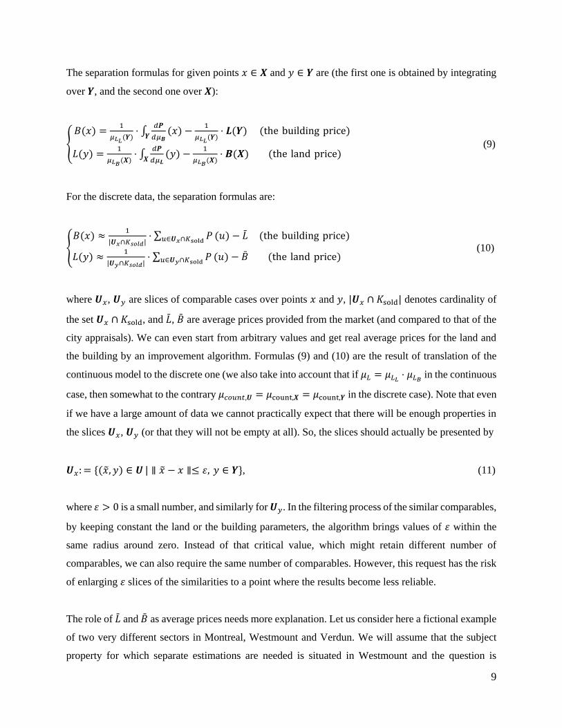
The separation formulas for given points 𝑥 ∈ 𝑿 and 𝑦 ∈ 𝒀 are (the first one is obtained by integrating

over 𝒀, and the second one over 𝑿):

{

𝐵(𝑥) =1

𝜇𝐿𝐿(𝒀)

⋅ ∫𝑑𝑷

𝑑𝜇𝑩𝒀(𝑥) −

1

𝜇𝐿𝐿(𝒀)

⋅ 𝑳(𝒀) (the building price)

𝐿(𝑦) =1

𝜇𝐿𝐵(𝑿)

⋅ ∫𝑑𝑷

𝑑𝜇𝑳𝑿(𝑦) −

1

𝜇𝐿𝐵(𝑿)

⋅ 𝑩(𝑿) (the land price) (9)

For the discrete data, the separation formulas are:

{𝐵(𝑥) ≈

1

|𝑼𝑥∩𝐾𝑠𝑜𝑙𝑑|⋅ ∑ 𝑃𝑢∈𝑼𝑥∩𝐾sold

(𝑢) − �̄� (the building price)

𝐿(𝑦) ≈1

|𝑼𝑦∩𝐾𝑠𝑜𝑙𝑑|⋅ ∑ 𝑃𝑢∈𝑼𝑦∩𝐾sold

(𝑢) − �̄� (the land price) (10)

where 𝑼𝑥, 𝑼𝑦 are slices of comparable cases over points 𝑥 and 𝑦, |𝑼𝑥 ∩ 𝐾sold| denotes cardinality of

the set 𝑼𝑥 ∩ 𝐾sold, and �̄�, �̄� are average prices provided from the market (and compared to that of the

city appraisals). We can even start from arbitrary values and get real average prices for the land and

the building by an improvement algorithm. Formulas (9) and (10) are the result of translation of the

continuous model to the discrete one (we also take into account that if 𝜇𝐿 = 𝜇𝐿𝐿⋅ 𝜇𝐿𝐵

in the continuous

case, then somewhat to the contrary 𝜇𝑐𝑜𝑢𝑛𝑡,𝑼 = 𝜇count,𝑿 = 𝜇count,𝒀 in the discrete case). Note that even

if we have a large amount of data we cannot practically expect that there will be enough properties in

the slices 𝑼𝑥, 𝑼𝑦 (or that they will not be empty at all). So, the slices should actually be presented by

𝑼𝑥: = {(�̃�, 𝑦) ∈ 𝑼 | ∥ �̃� − 𝑥 ∥≤ 𝜀,  𝑦 ∈ 𝒀}, (11)

where 𝜀 > 0 is a small number, and similarly for 𝑼𝑦. In the filtering process of the similar comparables,

by keeping constant the land or the building parameters, the algorithm brings values of 𝜀 within the

same radius around zero. Instead of that critical value, which might retain different number of

comparables, we can also require the same number of comparables. However, this request has the risk

of enlarging 𝜀 slices of the similarities to a point where the results become less reliable.

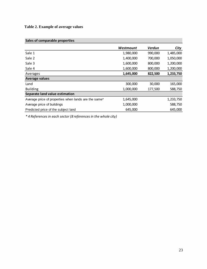
The role of �̄� and �̄� as average prices needs more explanation. Let us consider here a fictional example

of two very different sectors in Montreal, Westmount and Verdun. We will assume that the subject

property for which separate estimations are needed is situated in Westmount and the question is

10

whether the averages should be taken from Westmount or the whole city (here as being formed by

these two sectors in the following table).

When comparing various characteristics of the subject’s land in Westmount and those of all the lands

in the same sector, by letting building characteristics free, four very similar cases are found in the data.

Their average total price (e.g., $1.645 M) minus the average price of the buildings in the sector (e.g.,

$1 M) provides an estimate of $645 000. The estimation converges to the same value when the averages

of the total prices and the buildings in the whole city are considered (8 cases in the example). The role

of the averages here is just a fixed or “stable” point in the system. It allows separate value estimations,

expressing a better reading of the particular relation between the two components with an increased

number of comparable cases. Being too rigid with the averages in each sector (and even sub-sectors)

risks there having an insufficient density of comparables around them, which is required in the method.

The problem of interactions perhaps in favor of averages per sector also diminishes in the method by

successively keeping their appropriate parameters constant. A mathematical exposition on that issue

of a fixed point (and its improvement) is reported in the Appendix.

< Insert Table 2 >

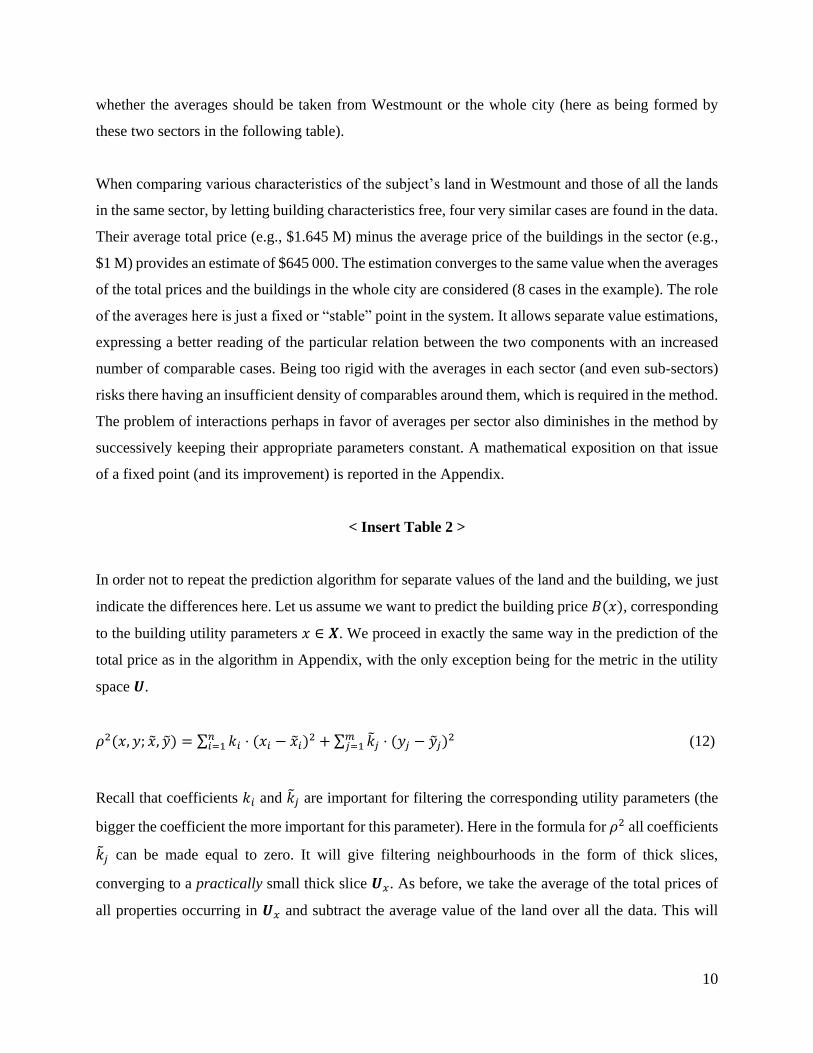
In order not to repeat the prediction algorithm for separate values of the land and the building, we just

indicate the differences here. Let us assume we want to predict the building price 𝐵(𝑥), corresponding

to the building utility parameters 𝑥 ∈ 𝑿. We proceed in exactly the same way in the prediction of the

total price as in the algorithm in Appendix, with the only exception being for the metric in the utility

space 𝑼.

𝜌2(𝑥, 𝑦; �̃�, �̃�) = ∑ 𝑘𝑖𝑛𝑖=1 ⋅ (𝑥𝑖 − �̃�𝑖)

2 + ∑ �̃�𝑗𝑚𝑗=1 ⋅ (𝑦𝑗 − �̃�𝑗)

2 (12)

Recall that coefficients 𝑘𝑖 and �̃�𝑗 are important for filtering the corresponding utility parameters (the

bigger the coefficient the more important for this parameter). Here in the formula for 𝜌2 all coefficients

�̃�𝑗 can be made equal to zero. It will give filtering neighbourhoods in the form of thick slices,

converging to a practically small thick slice 𝑼𝑥. As before, we take the average of the total prices of

all properties occurring in 𝑼𝑥 and subtract the average value of the land over all the data. This will

11

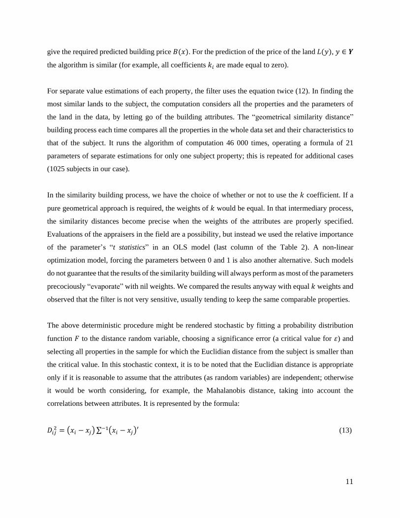
give the required predicted building price 𝐵(𝑥). For the prediction of the price of the land 𝐿(𝑦), 𝑦 ∈ 𝒀

the algorithm is similar (for example, all coefficients 𝑘𝑖 are made equal to zero).

For separate value estimations of each property, the filter uses the equation twice (12). In finding the

most similar lands to the subject, the computation considers all the properties and the parameters of

the land in the data, by letting go of the building attributes. The “geometrical similarity distance”

building process each time compares all the properties in the whole data set and their characteristics to

that of the subject. It runs the algorithm of computation 46 000 times, operating a formula of 21

parameters of separate estimations for only one subject property; this is repeated for additional cases

(1025 subjects in our case).

In the similarity building process, we have the choice of whether or not to use the 𝑘 coefficient. If a

pure geometrical approach is required, the weights of 𝑘 would be equal. In that intermediary process,

the similarity distances become precise when the weights of the attributes are properly specified.

Evaluations of the appraisers in the field are a possibility, but instead we used the relative importance

of the parameter’s “t statistics” in an OLS model (last column of the Table 2). A non-linear

optimization model, forcing the parameters between 0 and 1 is also another alternative. Such models

do not guarantee that the results of the similarity building will always perform as most of the parameters

precociously “evaporate” with nil weights. We compared the results anyway with equal 𝑘 weights and

observed that the filter is not very sensitive, usually tending to keep the same comparable properties.

The above deterministic procedure might be rendered stochastic by fitting a probability distribution

function 𝐹 to the distance random variable, choosing a significance error (a critical value for 𝜀) and

selecting all properties in the sample for which the Euclidian distance from the subject is smaller than

the critical value. In this stochastic context, it is to be noted that the Euclidian distance is appropriate

only if it is reasonable to assume that the attributes (as random variables) are independent; otherwise

it would be worth considering, for example, the Mahalanobis distance, taking into account the

correlations between attributes. It is represented by the formula:

𝐷𝑖𝑗 2 = (𝑥𝑖 − 𝑥𝑗)∑ (𝑥𝑖 − 𝑥𝑗)′

−1 (13)

12

where 𝑥𝑖, 𝑥𝑗 are the vectors of standardized parameters for properties 𝑖 and 𝑗 and ∑ is the variance-

covariance matrix of parameters for all properties. Vandell (1991) proposed an improved method,

which has been revised with more insights about this interesting subject of comparable property

selection (Gau et al., 1992, 1994; Lai et al., 2008).

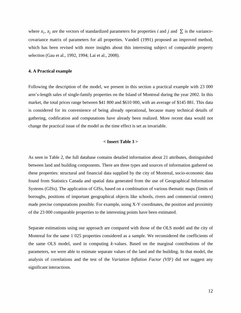
4. A Practical example

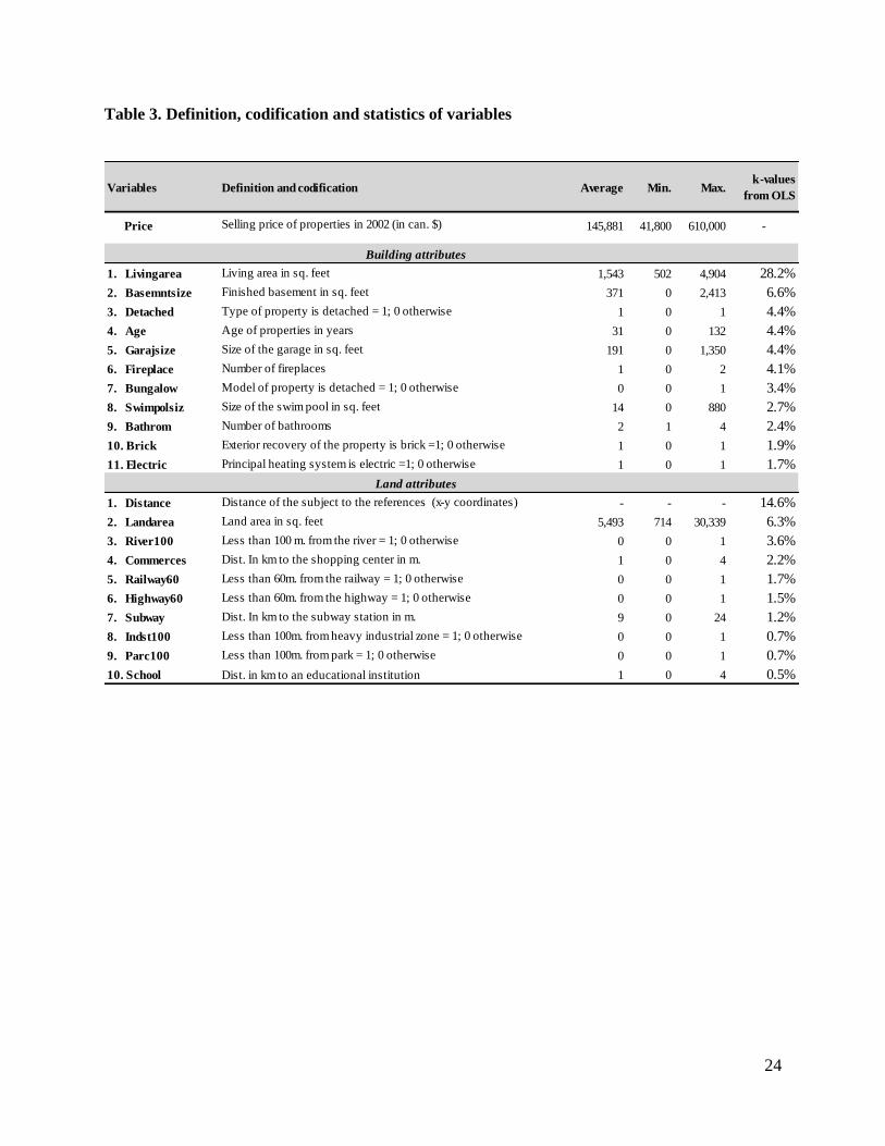
Following the description of the model, we present in this section a practical example with 23 000

arm’s-length sales of single-family properties on the Island of Montreal during the year 2002. In this

market, the total prices range between $41 800 and $610 000, with an average of $145 881. This data

is considered for its convenience of being already operational, because many technical details of

gathering, codification and computations have already been realized. More recent data would not

change the practical issue of the model as the time effect is set as invariable.

< Insert Table 3 >

As seen in Table 2, the full database contains detailed information about 21 attributes, distinguished

between land and building components. There are three types and sources of information gathered on

these properties: structural and financial data supplied by the city of Montreal, socio-economic data

found from Statistics Canada and spatial data generated from the use of Geographical Information

Systems (GISs). The application of GISs, based on a combination of various thematic maps (limits of

boroughs, positions of important geographical objects like schools, rivers and commercial centers)

made precise computations possible. For example, using X-Y coordinates, the position and proximity

of the 23 000 comparable properties to the interesting points have been estimated.

Separate estimations using our approach are compared with those of the OLS model and the city of

Montreal for the same 1 025 properties considered as a sample. We reconsidered the coefficients of

the same OLS model, used in computing 𝑘-values. Based on the marginal contributions of the

parameters, we were able to estimate separate values of the land and the building. In that model, the

analysis of correlations and the test of the Variation Inflation Factor (VIF) did not suggest any

significant interactions.

13

The second comparable base was the separate estimates produced by the City for the same properties

in the sample. Professionals use essentially the cost and the sales method to derive these estimates. It

is common for them to use a typical ratio in order to break down the observed total prices of properties

between the two components. This ratio is based on the study of the historical and recently observed

land prices, expressed per square foot for different areas throughout the city.

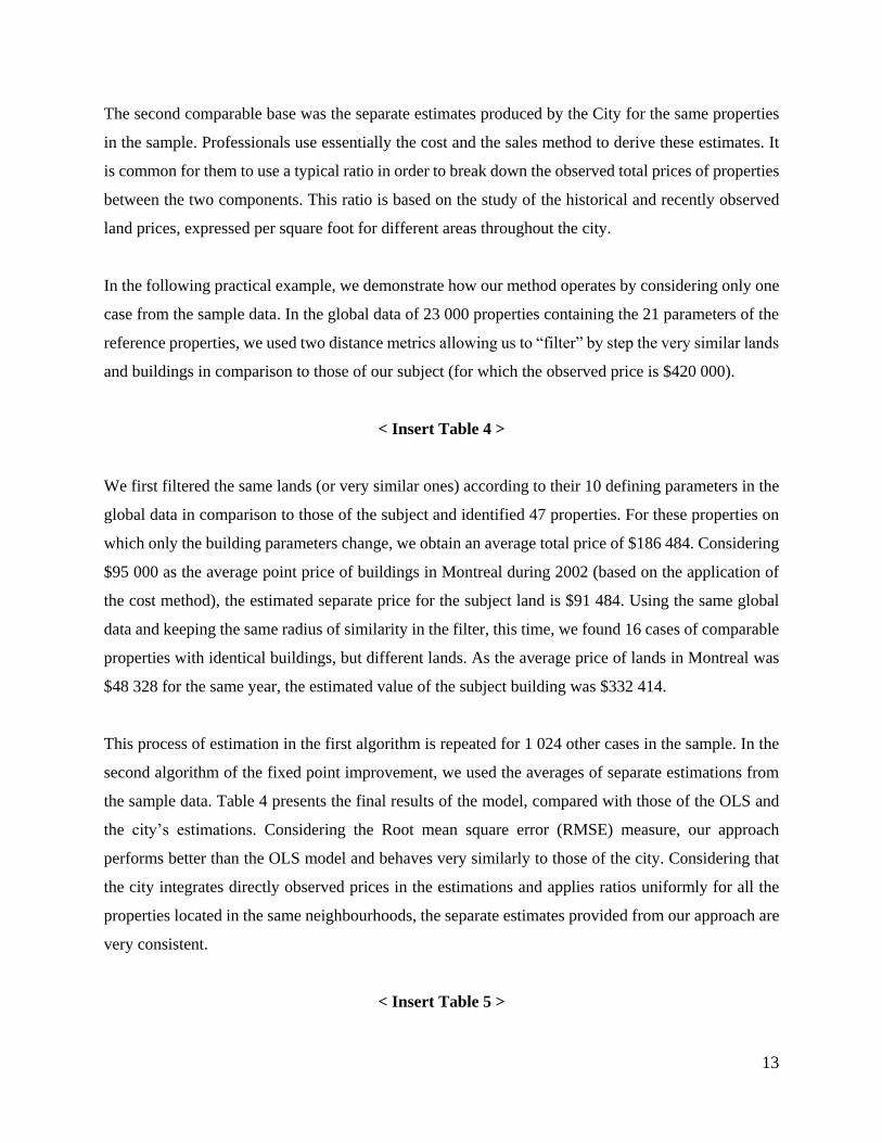
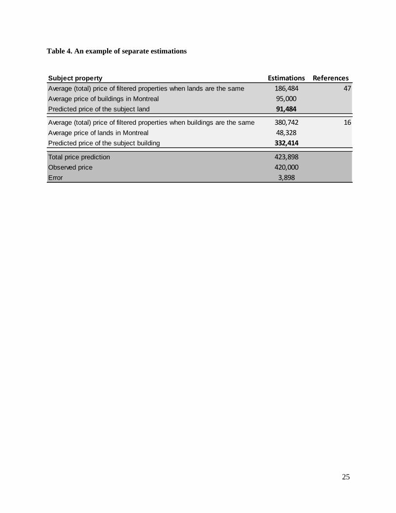
In the following practical example, we demonstrate how our method operates by considering only one

case from the sample data. In the global data of 23 000 properties containing the 21 parameters of the

reference properties, we used two distance metrics allowing us to “filter” by step the very similar lands

and buildings in comparison to those of our subject (for which the observed price is $420 000).

< Insert Table 4 >

We first filtered the same lands (or very similar ones) according to their 10 defining parameters in the

global data in comparison to those of the subject and identified 47 properties. For these properties on

which only the building parameters change, we obtain an average total price of $186 484. Considering

$95 000 as the average point price of buildings in Montreal during 2002 (based on the application of

the cost method), the estimated separate price for the subject land is $91 484. Using the same global

data and keeping the same radius of similarity in the filter, this time, we found 16 cases of comparable

properties with identical buildings, but different lands. As the average price of lands in Montreal was

$48 328 for the same year, the estimated value of the subject building was $332 414.

This process of estimation in the first algorithm is repeated for 1 024 other cases in the sample. In the

second algorithm of the fixed point improvement, we used the averages of separate estimations from

the sample data. Table 4 presents the final results of the model, compared with those of the OLS and

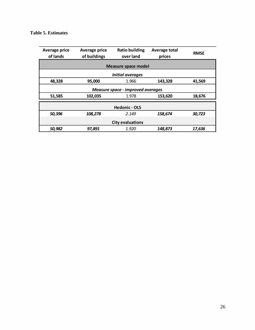
the city’s estimations. Considering the Root mean square error (RMSE) measure, our approach

performs better than the OLS model and behaves very similarly to those of the city. Considering that

the city integrates directly observed prices in the estimations and applies ratios uniformly for all the

properties located in the same neighbourhoods, the separate estimates provided from our approach are

very consistent.

< Insert Table 5 >

14

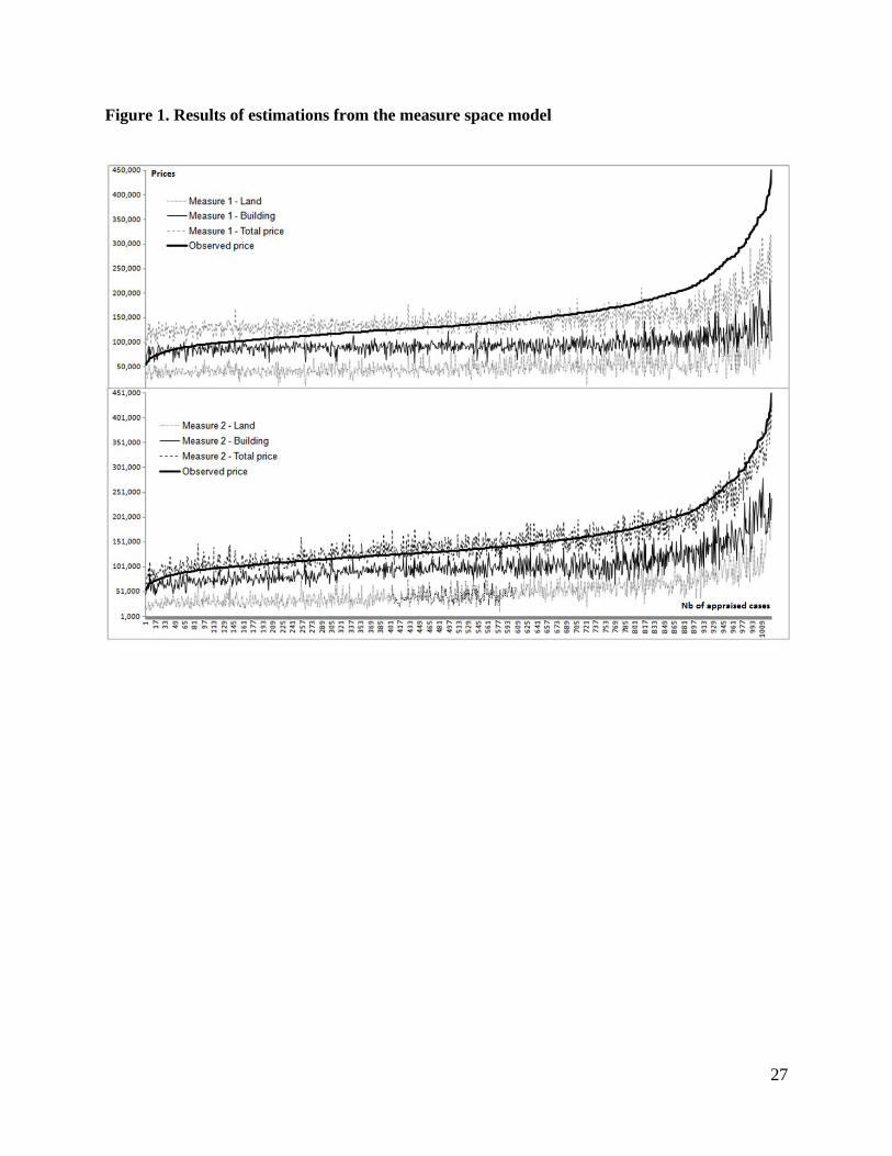
Even if the averages and the ratios of estimates from different models and sources are close for the

land and the building, the individual estimates are significantly different. Figure 1 shows the results of

our approach for all the estimates in the sample data. In the first step of the model, using averages from

the market as fixed points, estimated prices are far from the observed prices. But, in the next step, using

the improved averages from the results of the first algorithm, the estimations of the total prices are

shifted and better fit observed prices. It is noticeable also in both steps that the errors in the estimates

follow a small interval of errors, which slightly expand on the right side of the graphic (for expensive

properties).

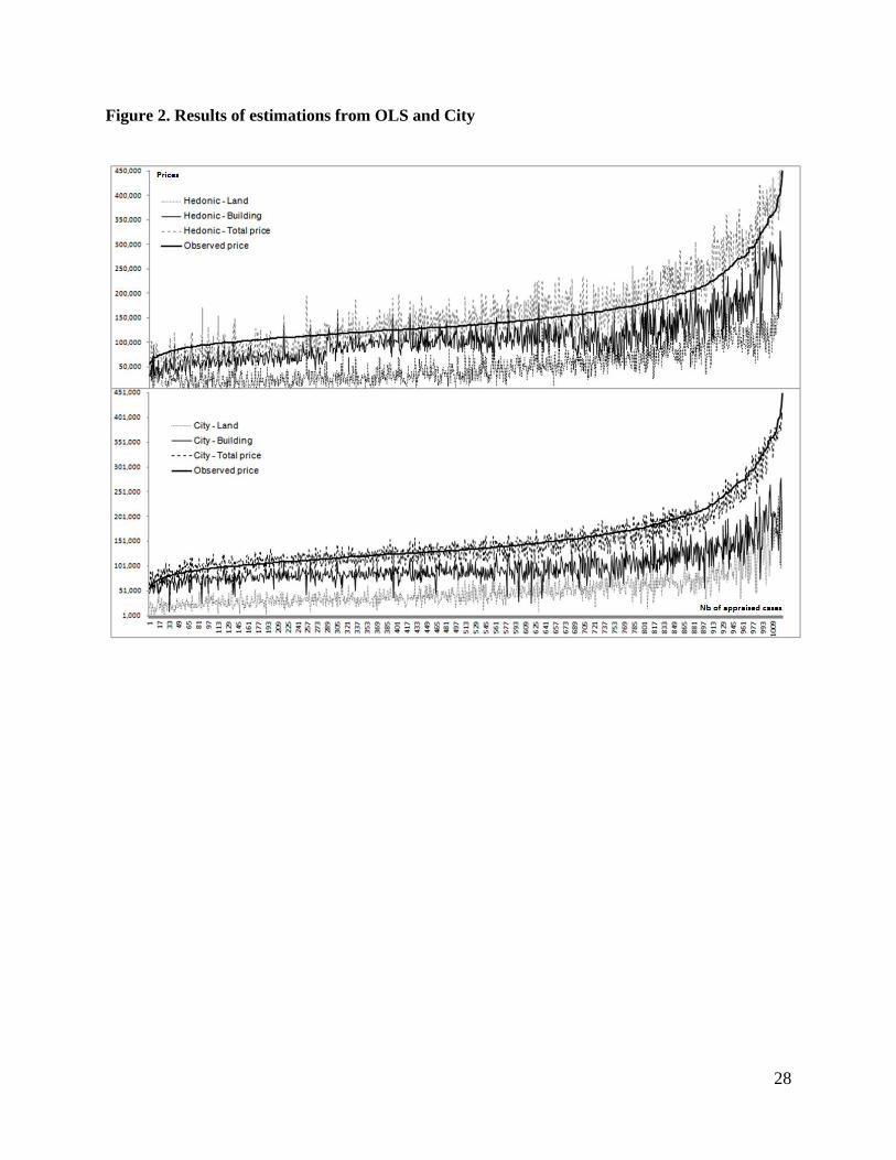
< Insert Figure 1 and Figure 2 >

In the case of the city’s estimates, we observe a similar pattern while distinguishing the distributions

of the errors in a constant smaller interval everywhere. The OLS model performs less well for the same

cases in the sample where the fluctuations of errors are mostly out of the tolerable range, for both total

and separate estimations.

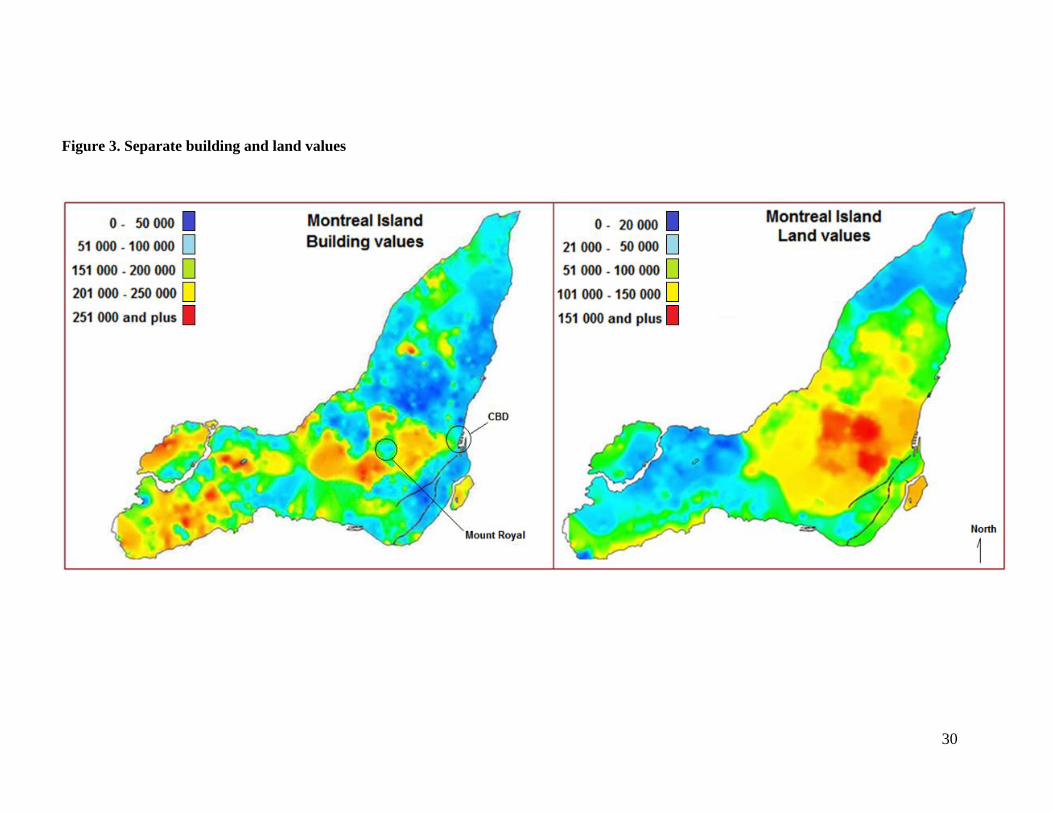
The results of the sample interpolated in the following map show interesting patterns. For example, as

expected, the building values are higher around the well-known markets encircling Mount Royal, while

also being high far away from downtown areas, especially in the west part of the city. Land values are

visibly higher in the center of the city, decreasing progressively towards the peripheral regions. There

are also higher land values in some sections along the border of the St. Lawrence River. The remarkable

information from the results and the map is the negative correlation between the two components: in

general, lands of higher value accommodate less expensive buildings, and vice versa.

< Insert Figure 3 >

These configurations are interesting for analyzing the specific dialectic between the land and the

building, in space but also in time. Are higher quality buildings placed on expensive or less expensive

lands? Is land value affecting the building or the inverse? What are the effects of different taxation

systems on the total or separate values? How do the values of the two components evolve in space and

time? When should buildings be demolished or improved? Accurate responses to such questions can

be provided only with separate estimations in practice.

15

5. Conclusion

Separate estimations for the land and the building are difficult to achieve in practice using approximate

methods. This situation raises more questions in the context of almost entirely built-up cities where

land transactions are scarce compared with low density residential properties. Even when there are

land transactions they are usually not reliable references for other usages with different characteristics.

In addition to practical difficulties, there is confusion from the theory and the academic fields where

opinions diverge. For authors defending the inseparability thesis, land and building components are

considered to be merged like an “omelette,” forming a new entity. For them, it is almost impossible

and even useless in practice to get separate values. From the opposite side, authors defend theoretically

the separability thesis and its practical necessity for different purposes without explaining how it can

be done.

In this paper, we have presented the bases for the separability thesis and provided an empirical solution

which can be used in practice, especially in the context of mass appraisals. To verify the applicability

and accuracy of our approach, we used detailed data for the cases of residential houses, and compared

them with the estimates of the city and the OLS model. From the strength of the results, it is

encouraging to observe that our approach provides a reliable alternative. In our practical example, it is

applied to the cases of single-family houses for which the issue is the most critical, but it can also be

used for other types of properties if sufficient data exists.

Obviously, no modeling effort can pretend to trace a clear-cut line of separation between the land and

the building values in practice. Debates on conceptual bases, interaction effects between the

parameters, allocation of a part of value to other types of agents like the Option and Business values

or the unexplainable part of the value in the model are some of the challenging aspects before the

important issue of price separation.

Existing approaches have different solutions and all of them face, as we do, these same challenging

questions. In comparison to the classical and OLS based methods, the use of the measure space theory

as presented here, combined with the remarkable progress in the quality of data and the capacity of

modern tools, increases expectations for accurate estimations of the land and the building values. It is

clear that the method presented can also integrate some intermediary steps, for example in comparable

16

property selection and combining the advantages of the hedonic regression model in estimating the

total or average values.

We approach the issue of separation in an objective way by proposing an original method that rests on

the use of measure theory in a geometric space representation. Its conceptual bases, mathematical

proofs and practical algorithms are presented by focusing on the price separation in the most direct

way. It is hoped that it will bring light to that issue, by “relaxing” more the strong resistance of the

inseparability thesis. The separate price estimation in practice will be of more concern in the future

when lands become rare (and more expensive), in a perspective of increasing consciousness of social

and environmental responsibilities.

17

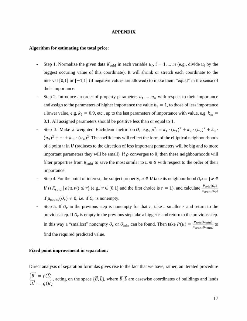
APPENDIX

Algorithm for estimating the total price:

- Step 1. Normalize the given data 𝐾sold in each variable 𝑢𝑖, 𝑖 = 1,… , 𝑛 (e.g., divide 𝑢𝑖 by the

biggest occuring value of this coordinate). It will shrink or stretch each coordinate to the

interval [0,1] or [−1,1] (if negative values are allowed) to make them “equal” in the sense of

their importance.

- Step 2. Introduce an order of property parameters 𝑢1, … , 𝑢𝑛 with respect to their importance

and assign to the parameters of higher importance the value 𝑘1 = 1, to those of less importance

a lower value, e.g. 𝑘2 = 0.9, etc., up to the last parameters of importance with value, e.g. 𝑘𝑚 =

0.1. All assigned parameters should be positive less than or equal to 1.

- Step 3. Make a weighted Euclidean metric on 𝑼, e.g., 𝜌2: = 𝑘1 ⋅ (𝑢1)2 + 𝑘2 ⋅ (𝑢2)

2 + 𝑘3 ⋅

(𝑢3)2 + ⋯+ 𝑘𝑚 ⋅ (𝑢𝑛)

2. The coefficients will reflect the form of the elliptical neighbourhoods

of a point 𝑢 in 𝑼 (radiuses to the direction of less important parameters will be big and to more

important parameters they will be small). If 𝜌 converges to 0, then these neighbourhoods will

filter properties from 𝐾sol𝑑 to save the most similar to 𝑢 ∈ 𝑼 with respect to the order of their

importance.

- Step 4. For the point of interest, the subject property, 𝑢 ∈ 𝑼 take its neighbourhood 𝑂𝑟: = {𝑤 ∈

𝑼 ∩ 𝐾sold | 𝜌(𝑢, 𝑤) ≤ 𝑟} (e.g., 𝑟 ∈ [0,1] and the first choice is 𝑟 = 1), and calculate 𝑷𝑠𝑜𝑙𝑑(𝑂𝑟)

𝜇𝑐𝑜𝑢𝑛𝑡(𝑂𝑟)

if 𝜇count(𝑂𝑟) ≠ 0, i.e. if 𝑂𝑟 is nonempty.

- Step 5. If 𝑂𝑟 in the previous step is nonempty for that 𝑟, take a smaller 𝑟 and return to the

previous step. If 𝑂𝑟 is empty in the previous step take a bigger 𝑟 and return to the previous step.

In this way a “smallest” nonempty 𝑂𝑟 or 𝑂min can be found. Then take 𝑃(𝑢) =𝑷𝑠𝑜𝑙𝑑(𝑂𝑚𝑖𝑛)

𝜇𝑐𝑜𝑢𝑛𝑡(𝑂𝑚𝑖𝑛) to

find the required predicted value.

Fixed point improvement in separation:

Direct analysis of separation formulas gives rise to the fact that we have, rather, an iterated procedure

{𝐵′⃗⃗ ⃗ = 𝑓(�⃗� )

𝐿′⃗⃗⃗ = 𝑔(�⃗� ), acting on the space {�⃗� , �⃗� }, where �⃗� , �⃗� are casewise coordinates of buildings and lands

18

over all given data. The prices being predicted (denote them (�⃗� 0, �⃗� 0)) are a fixed point on this map.

This is the unique fixed point, since the expressions for 𝑓 and 𝑔 are linear. The question is whether the

point (�⃗� 0, �⃗� 0) is stable (to make it possible to approximate it by the iterations starting from an arbitrary

point). Regardless of the fact of linearity of 𝑓 and 𝑔, the huge size and uncertain structure of the

corresponding matrix make it impossible to estimate its eigenvalues to solve the problem. However,

we will generally see a negative answer.

Since the divergence of the “differential” (𝑓(�⃗� ) − �⃗�

𝑔(�⃗� ) − �⃗� ) is obviously negative (and consequently,

Lebesgue measure on {�⃗� , �⃗� } is decreasing under the map), the fixed point (�⃗� 0, �⃗� 0) can only be

hyperbolic with a nonempty stable manifold through it. This is all that we can say about (�⃗� 0, �⃗� 0). The

fortunate occasion, proven by a numerical experiment, is that initial points (�⃗� , �⃗� ), such that

Average(𝑼𝑥 ∩ 𝐾sold) = �̄�, Average(𝑼𝑦 ∩ 𝐾𝑡𝑠𝑜𝑙𝑑) = �̄� (averages over all data), belong to the stable

manifold. As seen in the practical example, even the second iteration with these initial data gives a

significant improvement of the predictions. A practical implementation of the fixed point algorithm is

presented as follows.

- Step 1. Take initial values (�⃗� , �⃗� ), which are in the space of attraction of the fixed point (�⃗� 0, �⃗� 0).

As mentioned above, for the first iteration just interpret �̄�, �̄� in the separation formulas as total

averages over all the data (or the city).

- Step 2. Substitute the resulting values (𝐵′⃗⃗ ⃗ , 𝐿′⃗⃗⃗ ):= (𝑓(�⃗� ), 𝑔(�⃗� )) of the previous step to the same

formula (𝑓(𝐿′⃗⃗⃗ ), 𝑔(𝐵′⃗⃗ ⃗ )). It gives the second approximation.

- Step 3. If necessary, repeat step 2.

Note that repeating the iterations will not increase the accuracy of the prediction up to 100%, because

it is determined by the number of cases in the data. So, just two steps can be sufficient for a high

accuracy prediction. The other reason that not too many iterations should be taken is the fact that we

do not know for sure if the stable manifold 𝑀− is the total space. If it is not, there is a nonempty unstable

manifold 𝑀+. In this case the stable manifold plays the role of repeller and the unstable one that of

attractor. So, if the initial point is not exactly on 𝑀− (let it be an arbitrary small transversal shift from

it) then after several steps of approaching the fixed point (�⃗� 0, �⃗� 0) it will be unlimitedly going far away.

19

References

Anas, A. Taxes on buildings and land in a dynamic model of real estate markets, 2003, Working Paper:

EconWPA report No. 0302004.

Andelson, R. V. Land-value taxation around the world, Blackwell Publishers, 2000.

Appraisal Institute The appraisal of real estate (12th ed.). Chicago: Appraisal Institute, 2001.

Anselin, L. Local indicators of spatial association – LISA. Geographical Analysis, 1995, 27, 93-115

Arnott, R. and Petrova, P. (2002) The property tax as a tax and value: deadweight loss. National Bureau

of Economics, Working paper: 8913.

Balakrishnan, N. and Nevzorov, V. B. A Primer of Statistical Distributions, John Wiley&Sons, 2003.

Breiman, L. Statistical modeling: The two cultures. Statistical Science, 2001, 16:3, 199-231.

Brueckner, J. A. Modern analysis of the effects of site value taxation. National Tax Journal, 1986,

39:1, 49–58.

Clapp, J. M. A methodology for constructing vacant land price indices. AREUEA Journal, 1990, 18:3,

274–293.

Clapp, J. M, Jou, J. and Lee, T. Hedonic pricing with redevelopment options under uncertainty. Real

Estate Economics, 2012, 40, 197-216.

Colwell, P. F. A Primer on Piecewise Parabolic Multiple Regression Analysis via Estimations of

Chicago CBD Land Prices, Journal of Real Estate Finance and Economics, 1998, 17:1, 87-97.

Dancaescu, N. Assessment value to market value ratios in Alachua County, Fl: An examination using

GIS. Thesis, University of Florida, 2000.

Dorau, H. B. and Hinman, A. G. Urban Land Economics, McGrath Publishing Company, College Park,

Maryland, 1969.

Ely, T. R. Research in land and public utility economics. Land Economics, 1922, 1:1, 1–5.

Fischel, W. A. Municipal corporations, homeowners and the benefit view of the property tax. Research

paper, Lincoln Institute for Land Policy, 2000.

Fisher, E. M. Economic aspects of urban land use patterns. Journal of Industrial Economics, 1958, 6:3,

379–386.

Gau, G., Lai, T-Y. and Wang, K. Optimal Comparable Selection and Weighting in Real Property

Valuation: An Extension. Journal of the American Real Estate and Urban Economics Association,

1992, 20, 107–123.

Gau, G., T-Y. Lai, and K. Wang. A Further Discussion of Optimal Comparable Selection and

Weighting, and A Response to Green. Journal of the American Real Estate and Urban Economics

Association, 1994, 22, 655–663.

20

George, H. Progress and poverty (4th ed.). New York: Schalkenbach Foundation, 1975 [1898].

Gloudemans, R. J. An Empirical Analysis of the Incidence of Location on Land and Building Values,

Working Paper, Lincoln Institute of Land Policy, 2001.

Gloudemans, R. J. An empirical analysis of the incidence of location on land and building values.

Lincoln Institute of Land Policy, 2002, Working Paper: WP02RG2.

Guerin, B. G. MRA model development using vacant land and improved property in a single valuation

model. Assessment Journal, 2000, 7:4, 27–34.

Guofang, Z., Teruki, F. and Saburo, I. Effect of flooding on megalopolitan land prices: A case study

of the 2000 Tokai flood in Japan. Journal of Natural Disaster Science, 2003, 25:1, 23–36.

Halmos, P. R. Measure Theory, Springer-Verlag, 1974.

Hendriks, D. Apportionment in property valuation: Should we separate the inseparable? Journal of

Property Investment and Finance, 2005, 23:5, 455–470.

Isakson, H. R. An empirical analysis of the determinants of the value of vacant land. Journal of Real

Estate Research, 1997, 13:2, 103–114.

Keligian, D. L. Appraisal Issues Now Require Greater Attention for Tax Planning to Be Effective.

Journal of Taxation, 1994, 80:2, 98-103.

Kitchen, H. Property taxation: Issues in implementation. Working paper, Trent University,

Peterborough, Ontario, 2003.

Lai, T.-Y., Vandell, K., Wang, K., and Welke, G. Estimating Property Values by Replication: An

Alternative to the Traditional Grid and Regression Methods. Journal of Real Estate Research, 2008,

30:4, 441-460.

Lancaster, K. J. A new approach to consumer theory. Journal of Political Economy, 1966, 74:2, 132–

157.

Marshall, A. Principles of economics. London: Macmillan, 1992.

Martin, R. S. and Nafe, S. D. Segregating real estate value from nonrealty value in shopping centers,

Appraisal Journal, 1996, 64:1 1-13.

Mills, E. S. Is land taxation practical? University of Illinois, Real Estate Letter, 1998, 12:4, 1–5.

Miller, N. G., Jones, S. T. and Roulac, S. E. In defense of the Land Residual Theory and the Absence

of a Business Value Component for Retail Property, Journal of Real Estate Research, 1995, 10:2, 203-

215.

Oates, W. E. and Schwab, R. M. The impact of urban land taxation: The Pittsburgh experience.

National Tax Journal, 1997, 50:1, 1–22.

Ohno, K. Preparation and Use of Land Value Maps. Appraisal Journal, 1985, 53:2, 262-268.

21

Özdilek, Ü. An overview of the enquiries on the issue of apportionment of value between land and

improvements. Journal of Property Research, 2012, 29:1, 69-84.

Pavlov, A. D. Space-Varying Regression Coefficients: A Semi-Parametric Approach Applied to Real

Estate Markets, Real Estate Economics, 2000, 28:2, 249-283.

Plassmann, F. and Tideman, N. T. A framework for assessing the value of downtown land. Working

paper e07-5, Virginia Polytechnic Institute and State University, 2003.

Plaut, P. O. and Plaut, S. E. Decisions to renovate and to move. Journal of Real Estate Research, 2010,

32, 461-484.

Quigg, L. Empirical testing of real-option pricing models. Journal of Finance, 1993, 48:2, 621-640.

Rabianski, J. S. Going-concern value, market value, and intangible value, Appraisal Journal, 1996,

64:), 184-194.

Ratcliff, R. U. Net income can’t be split. Appraisal Journal, 1950, 18:1, 168–172.

Rice, H. The Value of Developed Land Considered Vacant and Unimproved, 1997, Real Estate Review.

Robinson, J. A. Note on the apportionment of value between land and improvements. RICS Research

Conference, University of Melbourne, 1999.

Rosen, S. M. Hedonic prices and implicit markets: Product differentiation in pure competition. Journal

of Political Economy, 1974, 82:1, 34–55.

Royden, H. L. Real Analysis, Macmillan Publishing Company, 1988.

Russell, B. History of Western Philosophy. London: G. Allen and Unwin, 1945.

Shi, S. The Improved Net Rate Analysis, Journal of Real Estate Research (Forthcoming paper).

Sirmans, S. G., MacPherson, D. A. and Zietz, E. N. The composition of hedonic pricing models.

Journal of Real Estate Literature, 2005, 13:1, 3–47.

Smith, A. An Inquiry into the Nature and Causes of the Wealth of Nations, Modern Library, New York,

1886.

Stokes, J. R. and Cox, A. T. The Speculative Value of Farm Real Estate, Journal of Real Estate

Research (Forthcoming paper).

Vandell, K. Optimal Comparable Selection and Weighting in Real Property Valuation. Journal of the

American Real Estate and Urban Economics Association, 1991, 19, 213–239.

Williams, J. T. Real estate development as an option, Journal of Real Estate Finance and Economics,

1991, 4, 191-208.

22

Table 1 - Various price apportionment methods

Apportionment theories Techniques Methods

1.1 Allocation

1.2 Abstraction

1.3 Extraction

2.1 Subdivision

2.2 Land residual

2.3 Ground rent

3.1 Direct comparison

3.2 OLS modeling

3.3 Geometric modeling

1. Fractional Apportionment Theory (FAT)

2. Rent Apportionment Theory (RAT)

Cost, Price

Income

Price3. Price Apportionment Theory (PAT)

23

Table 2. Example of average values

Westmount Verdun City

Sale 1 1,980,000 990,000 1,485,000

Sale 2 1,400,000 700,000 1,050,000

Sale 3 1,600,000 800,000 1,200,000

Sale 4 1,600,000 800,000 1,200,000

Averages 1,645,000 822,500 1,233,750

Land 300,000 30,000 165,000

Building 1,000,000 177,500 588,750

Average price of properties when lands are the same* 1,645,000 1,233,750

Average price of buildings 1,000,000 588,750

Predicted price of the subject land 645,000 645,000

* 4 References in each sector (8 references in the whole city)

Sales of comparable properties

Average values

Separate land value estimation

24

Table 3. Definition, codification and statistics of variables

Variables Definition and codification Average Min. Max.k-values

from OLS

Price Selling price of properties in 2002 (in can. $) 145,881 41,800 610,000 -

1. Livingarea Living area in sq. feet 1,543 502 4,904 28.2%

2. Basemntsize Finished basement in sq. feet 371 0 2,413 6.6%

3. Detached Type of property is detached = 1; 0 otherwise 1 0 1 4.4%

4. Age Age of properties in years 31 0 132 4.4%

5. Garajsize Size of the garage in sq. feet 191 0 1,350 4.4%

6. Fireplace Number of fireplaces 1 0 2 4.1%

7. Bungalow Model of property is detached = 1; 0 otherwise 0 0 1 3.4%

8. Swimpolsiz Size of the swim pool in sq. feet 14 0 880 2.7%

9. Bathrom Number of bathrooms 2 1 4 2.4%

10. Brick Exterior recovery of the property is brick =1; 0 otherwise 1 0 1 1.9%

11. Electric Principal heating system is electric =1; 0 otherwise 1 0 1 1.7%

1. Distance Distance of the subject to the references (x-y coordinates) - - - 14.6%

2. Landarea Land area in sq. feet 5,493 714 30,339 6.3%

3. River100 Less than 100 m. from the river = 1; 0 otherwise 0 0 1 3.6%

4. Commerces Dist. In km to the shopping center in m. 1 0 4 2.2%

5. Railway60 Less than 60m. from the railway = 1; 0 otherwise 0 0 1 1.7%

6. Highway60 Less than 60m. from the highway = 1; 0 otherwise 0 0 1 1.5%

7. Subway Dist. In km to the subway station in m. 9 0 24 1.2%

8. Indst100 Less than 100m. from heavy industrial zone = 1; 0 otherwise 0 0 1 0.7%

9. Parc100 Less than 100m. from park = 1; 0 otherwise 0 0 1 0.7%

10. School Dist. in km to an educational institution 1 0 4 0.5%

Building attributes

Land attributes

25

Table 4. An example of separate estimations

Subject property Estimations References

Average (total) price of filtered properties when lands are the same 186,484 47

Average price of buildings in Montreal 95,000

Predicted price of the subject land 91,484

Average (total) price of filtered properties when buildings are the same 380,742 16

Average price of lands in Montreal 48,328

Predicted price of the subject building 332,414

Total price prediction 423,898

Observed price 420,000

Error 3,898

26

Table 5. Estimates

Average price

of lands

Average price

of buildings

Ratio building

over land

Average total

pricesRMSE

48,328 95,000 1.966 143,328 41,569

51,585 102,035 1.978 153,620 18,676

50,396 108,278 2.149 158,674 30,723

50,982 97,891 1.920 148,873 17,636

Hedonic - OLS

Measure space model

Measure space - improved averages

City evaluations

Initial averages

27

Figure 1. Results of estimations from the measure space model

28

Figure 2. Results of estimations from OLS and City

30

Figure 3. Separate building and land values