propensity score methods, models and adjustment...propensity score methods, models and adjustment dr...
TRANSCRIPT

Propensity Score Methods, Models andAdjustment
Dr David A. Stephens
Department of Mathematics & StatisticsMcGill University
Montreal, QC, Canada.
[email protected]/dstephens/SISCR2016/
1
Part 1: Introduction
1.1 The central causal question1.2 Notation1.3 Causal estimands1.4 Basics of estimation1.5 The Monte Carlo paradigm1.6 Collapsibility1.7 The randomized study1.8 Confounding1.9 Statistical modelling
2
Part 2: The Propensity Score
2.1 Manufacturing balance2.2 The propensity score for binary exposures2.3 Matching via the propensity score2.4 The Generalized Propensity Score2.5 Propensity score regression2.6 Adjustment by weighting2.7 Augmentation and double robustness
3
Part 3: Implementation and Computation
3.1 Statistical tools3.2 Key considerations
4

Part 4: Extensions
4.1 Longitudinal studies4.2 The Marginal Structural Model (MSM)
5

Part 5: New Directions
5.1 New challenges5.2 Bayesian approaches
6

Part 1
Introduction
7

The central causal question
In many research domains, the objective of an investigation isto quantify the effect on a measurable outcome of changing oneof the conditions under which the outcome is measured.
I in a health research setting, we may wish to discover thebenefits of a new therapy compared to standard care;
I in economics, we may wish to study the impact of atraining programme on the wages of unskilled workers;
I in transportation, we may attempt to understand the effectof embarking upon road building schemes on traffic flow ordensity in a metropolitan area.
The central statistical challenge is that, unless the condition ofinterest is changed independently, the inferred effect may besubject to the influence of other variables.
1.1: The central causal question 8
The central causal question
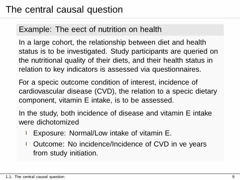
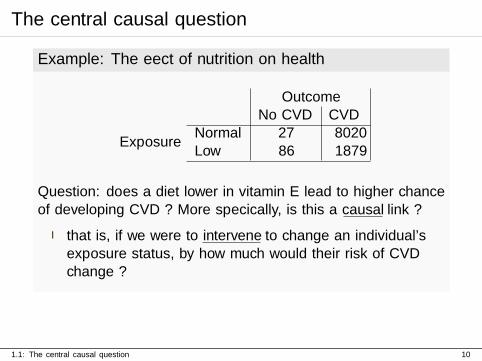
Example: The effect of nutrition on health
In a large cohort, the relationship between diet and healthstatus is to be investigated. Study participants are queried onthe nutritional quality of their diets, and their health status inrelation to key indicators is assessed via questionnaires.
For a specific outcome condition of interest, incidence ofcardiovascular disease (CVD), the relation to a specific dietarycomponent, vitamin E intake, is to be assessed.
In the study, both incidence of disease and vitamin E intakewere dichotomized
I Exposure: Normal/Low intake of vitamin E.
I Outcome: No incidence/Incidence of CVD in five yearsfrom study initiation.
1.1: The central causal question 9
The central causal question
Example: The effect of nutrition on health
OutcomeNo CVD CVD
ExposureNormal 27 8020Low 86 1879
Question: does a diet lower in vitamin E lead to higher chanceof developing CVD ? More specifically, is this a causal link ?
I that is, if we were to intervene to change an individual’sexposure status, by how much would their risk of CVDchange ?
1.1: The central causal question 10
The language of causal inference
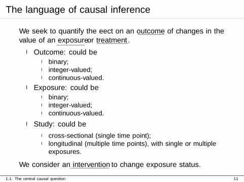
We seek to quantify the effect on an outcome of changes in thevalue of an exposure or treatment.
I Outcome: could beI binary;I integer-valued;I continuous-valued.
I Exposure: could beI binary;I integer-valued;I continuous-valued.
I Study: could be
I cross-sectional (single time point);I longitudinal (multiple time points), with single or multiple
exposures.
We consider an intervention to change exposure status.
1.1: The central causal question 11
Notation
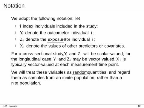
We adopt the following notation: let
I i index individuals included in the study;
I Yi denote the outcome for individual i;
I Zi denote the exposure for individual i;
I Xi denote the values of other predictors or covariates.
For a cross-sectional study, Yi and Zi will be scalar-valued; forthe longitudinal case, Yi and Zi may be vector valued. Xi istypically vector-valued at each measurement time point.
We will treat these variables as random quantities, and regardthem as samples from an infinite population, rather than afinite population.
1.2: Notation 12

Counterfactual or Potential Outcomes
In order to phrase causal questions of interest, it is useful toconsider certain hypothetical outcome quantities that representthe possible outcomes under different exposure alternatives.
We denote byYi(z)
the hypothetical outcome for individual i if we intervene to setexposure to z.
Yi(z) is termed a counterfactual or potential outcome.
1.2: Notation 13
Counterfactual or Potential Outcomes
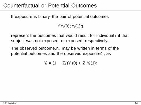
If exposure is binary, the pair of potential outcomes
{Yi(0), Yi(1)}
represent the outcomes that would result for individual i if thatsubject was not exposed, or exposed, respectively.
The observed outcome, Yi, may be written in terms of thepotential outcomes and the observed exposure, Zi, as
Yi = (1− Zi)Yi(0) + ZiYi(1).
1.2: Notation 14
Counterfactual or Potential Outcomes
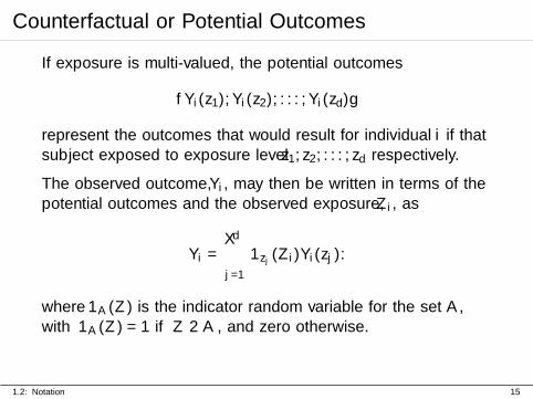
If exposure is multi-valued, the potential outcomes
{Yi(z1), Yi(z2), . . . , Yi(zd)}
represent the outcomes that would result for individual i if thatsubject exposed to exposure level z1, z2, . . . , zd respectively.
The observed outcome, Yi, may then be written in terms of thepotential outcomes and the observed exposure, Zi, as
Yi =
d∑j=1
1zj (Zi)Yi(zj).
where 1A(Z) is the indicator random variable for the set A,with 1A(Z) = 1 if Z ∈ A, and zero otherwise.
1.2: Notation 15
Counterfactual or Potential Outcomes
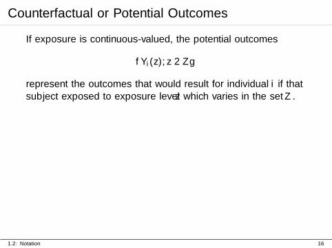
If exposure is continuous-valued, the potential outcomes
{Yi(z), z ∈ Z}
represent the outcomes that would result for individual i if thatsubject exposed to exposure level z which varies in the set Z.
1.2: Notation 16
Counterfactual or Potential Outcomes
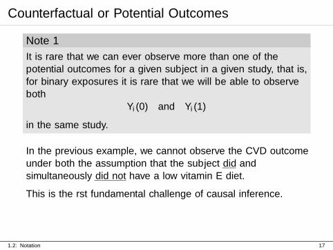
Note 1
It is rare that we can ever observe more than one of thepotential outcomes for a given subject in a given study, that is,for binary exposures it is rare that we will be able to observeboth
Yi(0) and Yi(1)
in the same study.
In the previous example, we cannot observe the CVD outcomeunder both the assumption that the subject did andsimultaneously did not have a low vitamin E diet.
This is the first fundamental challenge of causal inference.
1.2: Notation 17
Causal Estimands
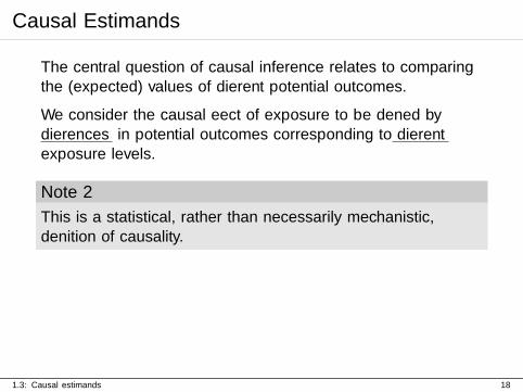
The central question of causal inference relates to comparingthe (expected) values of different potential outcomes.
We consider the causal effect of exposure to be defined bydifferences in potential outcomes corresponding to differentexposure levels.
Note 2
This is a statistical, rather than necessarily mechanistic,definition of causality.
1.3: Causal estimands 18
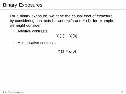
Binary Exposures
For a binary exposure, we define the causal effect of exposureby considering contrasts between Yi(0) and Yi(1); for example,we might consider
I Additive contrastsYi(1)− Yi(0)
I Multiplicative contrasts
Yi(1)/Yi(0)
1.3: Causal estimands 19
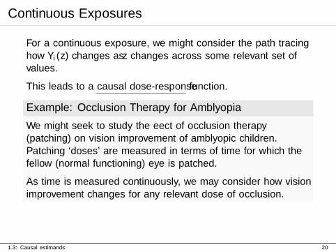
Continuous Exposures
For a continuous exposure, we might consider the path tracinghow Yi(z) changes as z changes across some relevant set ofvalues.
This leads to a causal dose-response function.
Example: Occlusion Therapy for Amblyopia
We might seek to study the effect of occlusion therapy(patching) on vision improvement of amblyopic children.Patching ‘doses’ are measured in terms of time for which thefellow (normal functioning) eye is patched.
As time is measured continuously, we may consider how visionimprovement changes for any relevant dose of occlusion.
1.3: Causal estimands 20
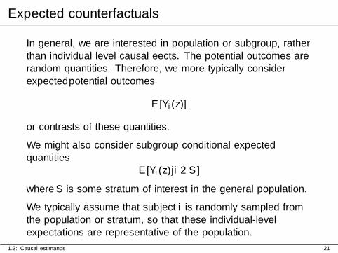
Expected counterfactuals
In general, we are interested in population or subgroup, ratherthan individual level causal effects. The potential outcomes arerandom quantities. Therefore, we more typically considerexpected potential outcomes
E[Yi(z)]
or contrasts of these quantities.
We might also consider subgroup conditional expectedquantities
E[Yi(z)|i ∈ S]
where S is some stratum of interest in the general population.
We typically assume that subject i is randomly sampled fromthe population or stratum, so that these individual-levelexpectations are representative of the population.
1.3: Causal estimands 21
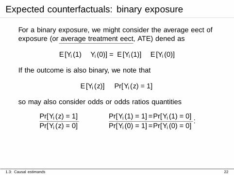
Expected counterfactuals: binary exposure
For a binary exposure, we might consider the average effect ofexposure (or average treatment effect, ATE) defined as
E[Yi(1)− Yi(0)] = E[Yi(1)]−E[Yi(0)]
If the outcome is also binary, we note that
E[Yi(z)] ≡ Pr[Yi(z) = 1]
so may also consider odds or odds ratios quantities
Pr[Yi(z) = 1]
Pr[Yi(z) = 0]
Pr[Yi(1) = 1]/Pr[Yi(1) = 0]
Pr[Yi(0) = 1]/Pr[Yi(0) = 0].
1.3: Causal estimands 22
Expected counterfactuals: binary exposure
We may also consider quantities such as the
average treatment effect on the treated, ATT
defined asE[Yi(1)− Yi(0)|Zi = 1]
although such quantities can be harder to interpret.
The utility of the potential outcomes formulation is evident inthis definition.
1.3: Causal estimands 23

Example: antidepressants and autism
Antidepressants are quite widely prescribed and for a variety ofmental health concerns. However, patients can be reluctant toembark on a course of antidepressants during pregnancy. Wemight wish to investigate, in a population of users (andpotentials users) of antidepressants, the incidence ofautism-spectrum disorder in early childhood and to assess thecausal influence of antidepressant use on this incidence.
I Outcome: binary, recording the a diagnosis ofautism-spectrum disorder in the child by age 5;
I Exposure: antidepressant use during 2nd or 3rd trimesterof pregnancy.
Then we may wish to quantity
E[Yi(antidepressant)−Yi(no antidepressant)|Antidep. actually used].
1.3: Causal estimands 24
Estimation of average potential outcomes
We wish to obtain estimates of causal quantities of interestbased on the available data, which typically constitute arandom sample from the target population.
We may apply to standard statistical principles to achieve theestimation. Typically, we will use sample mean type quantities:for a random sample of size n, the sample mean
1
n
n∑i=1
Yi
is an estimator of the population mean and so on.
1.4: Basics of estimation 25
Estimation of average potential outcomes
In a typical causal setting, we wish to perform estimation ofaverage potential outcome (APO) values.
Consider first the situation where all subjects in a randomsample receive a given exposure z; we wish to estimate E[Y (z)].
In terms of a formal probability calculation, we write this as
E[Y (z)] =
∫y fY (z)(y) dy
=
∫y fY (z),X(y, x) dy dx
where the second line recognizes that in the population, thevalues of the predictors X vary randomly according to someprobability distribution
1.4: Basics of estimation 26
Estimation of average potential outcomes
I fY (z)(y) is the marginal distribution of the potentialoutcome when we set the exposure to z.
I fY (z),X(y, x) is the joint distribution of (Y (z), X) in thepopulation where we set the exposure to z.
Note that we may also write
E[Y (z)] =
∫y1z(z) fY (z),X(y, x) dy dz dx
that is, imagining an exposure distribution degenerate at z = z.Our random sample is from the population with density
1z(z) fY (z),X(y, x) ≡ 1z(z) fY |Z,X(y|z, x)fX(x).
1.4: Basics of estimation 27
Estimation of average potential outcomes
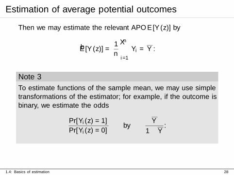
Then we may estimate the relevant APO E[Y (z)] by
E[Y (z)] =1
n
n∑i=1
Yi = Y .
Note 3
To estimate functions of the sample mean, we may use simpletransformations of the estimator; for example, if the outcome isbinary, we estimate the odds
Pr[Yi(z) = 1]
Pr[Yi(z) = 0]by
Y
1− Y.
1.4: Basics of estimation 28

Monte Carlo methods
Causal quantities are typically average measures across a givenpopulation, hence we often need to consider integrals withrespect to probability distributions.
Recall a simplified version of the calculation above: for anyfunction g(.), we have
E[g(Y )] =
∫g(y) fY (y) dy
=
∫g(y) fY,X(y, x) dy dx
Rather than performing this calculation analytically usingintegration, we may consider approximating it numericallyusing Monte Carlo.
1.5: The Monte Carlo paradigm 29
Monte Carlo methods
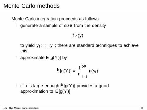
Monte Carlo integration proceeds as follows:
I generate a sample of size n from the density
fY (y)
to yield y1, . . . , yn; there are standard techniques to achievethis.
I approximate E[g(Y )] by
E[g(Y )] =1
n
n∑i=1
g(yi).
I if n is large enough, E[g(Y )] provides a goodapproximation to E[g(Y )]
1.5: The Monte Carlo paradigm 30
Monte Carlo methods
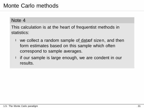
Note 4
This calculation is at the heart of frequentist methods instatistics:
I we collect a random sample of data of size n, and thenform estimates based on this sample which oftencorrespond to sample averages.
I if our sample is large enough, we are confident in ourresults.
1.5: The Monte Carlo paradigm 31
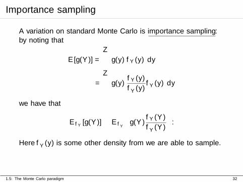
Importance sampling
A variation on standard Monte Carlo is importance sampling:by noting that
E[g(Y )] =
∫g(y) fY (y) dy
=
∫g(y)
fY (y)
f∗Y (y)f∗Y (y) dy
we have that
EfY [g(Y )] ≡ Ef∗Y
[g(Y )
fY (Y )
f∗Y (Y )
].
Here f∗Y (y) is some other density from we are able to sample.
1.5: The Monte Carlo paradigm 32
Importance sampling
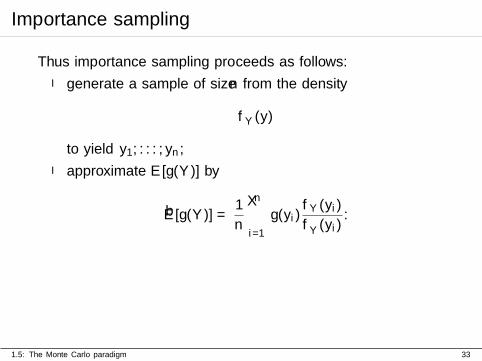
Thus importance sampling proceeds as follows:
I generate a sample of size n from the density
f∗Y (y)
to yield y1, . . . , yn;
I approximate E[g(Y )] by
E[g(Y )] =1
n
n∑i=1
g(yi)fY (yi)
f∗Y (yi).
1.5: The Monte Carlo paradigm 33
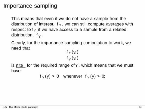
Importance sampling
This means that even if we do not have a sample from thedistribution of interest, fY , we can still compute averages withrespect to fY if we have access to a sample from a relateddistribution, f∗Y .
Clearly, for the importance sampling computation to work, weneed that
fY (yi)
f∗Y (yi)
is finite for the required range of Y , which means that we musthave
f∗Y (y) > 0 whenever fY (y) > 0.
1.5: The Monte Carlo paradigm 34
Marginal and conditional measures of effect
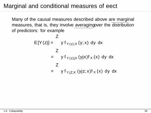
Many of the causal measures described above are marginalmeasures, that is, they involve averaging over the distributionof predictors: for example
E[Y (z)] =
∫y fY (z),X(y, x) dy dx
=
∫y fY (z)|X(y|x)fX(x) dy dx
=
∫y fY |Z,X(y|z, x)fX(x) dy dx
1.6: Collapsibility 35
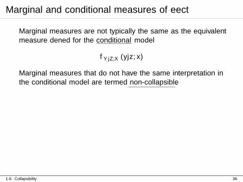
Marginal and conditional measures of effect
Marginal measures are not typically the same as the equivalentmeasure defined for the conditional model
fY |Z,X(y|z, x)
Marginal measures that do not have the same interpretation inthe conditional model are termed non-collapsible.
1.6: Collapsibility 36

Example: logistic regression
Consider the binary response, binary exposure regressionmodel, where
Pr[Y = 1|Z = z,X = x] =exp{β0 + β1z + β2x}
1 + exp{β0 + β1z + β2x}= µ(z, x;β)
say. We then have that in this conditional (on x) model, theparameter
β1 = log
(Pr[Y = 1|Z = 1, X = x]/Pr[Y = 0|Z = 1, X = x]
Pr[Y = 1|Z = 0, X = x]/Pr[Y = 0|Z = 0, X = x]
)is the log odds ratio comparing outcome probabilities with forZ = 1 and Z = 0 respectively.
1.6: Collapsibility 37
Example: logistic regression
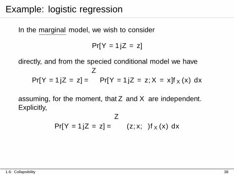
In the marginal model, we wish to consider
Pr[Y = 1|Z = z]
directly, and from the specified conditional model we have
Pr[Y = 1|Z = z] =
∫Pr[Y = 1|Z = z,X = x]fX(x) dx
assuming, for the moment, that Z and X are independent.Explicitly,
Pr[Y = 1|Z = z] =
∫µ(z, x;β)fX(x) dx
1.6: Collapsibility 38

Example: logistic regression
Typically, the integral that defines Pr[Y = 1|Z = z] in this wayis not tractable. However, as, Y is binary, we may still considera logistic regression model in the marginal distribution, sayparameterized as
Pr[Y = 1|Z = z] =exp{θ0 + θ1z}
1 + exp{θ0 + θ1z}
where θ1 is the marginal log odds ratio.
In general, β1 6= θ1.
1.6: Collapsibility 39
The randomized study
The approach that intervenes to set exposure equal to z for allsubjects, however, does not facilitate comparison of APOs fordifferent values of z.
Therefore consider a study design based on randomization;consider from simplicity the binary exposure case. Suppose thata random sample of size 2n is obtained, and split into two equalparts.
I the first group of n are assigned the exposure and form the‘treated’ sample,
I the second half are left ‘untreated’.
1.7: The randomized study 40
The randomized study
For both the treated and untreated groups we may use theprevious logic, and estimate the ATE
E[Yi(1)− Yi(0)] = E[Yi(1)]−E[Yi(0)]
by the difference in means in the two groups, that is
1
n
n∑i=1
Yi −1
n
2n∑i=n+1
Yi.
The key idea here is that the two halves of the original sampleare exchangeable with respect to their properties; the onlysystematic difference between them is due to exposureassignment.
1.7: The randomized study 41
The randomized study
In a slightly modified design, suppose that we obtain a randomsample of size n from the study population, but then assignexposure randomly to subjects in the sample: subject i receivestreatment with probability p.
I if p = 1/2, then there is an equal chance of receivingtreatment or not;
I we may choose any value of 0 < p < 1.
In the final sample, the number treated, n1, is a realization of arandom variable N1 where
N1 ∼ Binomial(n, p).
1.7: The randomized study 42
The randomized study
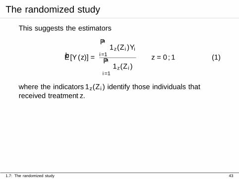
This suggests the estimators
E[Y (z)] =
n∑i=1
1z(Zi)Yi
n∑i=1
1z(Zi)
z = 0, 1 (1)
where the indicators 1z(Zi) identify those individuals thatreceived treatment z.
1.7: The randomized study 43
The randomized study
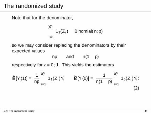
Note that for the denominator,
n∑i=1
11(Zi) ∼ Binomial(n, p)
so we may consider replacing the denominators by theirexpected values
np and n(1− p)
respectively for z = 0, 1. This yields the estimators
E[Y (1)] =1
np
n∑i=1
11(Zi)Yi E[Y (0)] =1
n(1− p)
n∑i=1
10(Zi)Yi.
(2)
1.7: The randomized study 44
The randomized study
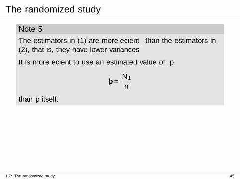
Note 5
The estimators in (1) are more efficient than the estimators in(2), that is, they have lower variances.
It is more efficient to use an estimated value of p
p =N1
n
than p itself.
1.7: The randomized study 45
The randomized study
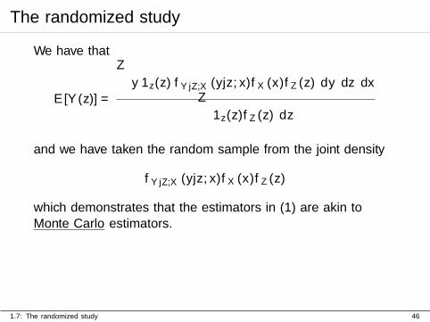
We have that
E[Y (z)] =
∫y 1z(z) fY |Z,X(y|z, x)fX(x)fZ(z) dy dz dx∫
1z(z)fZ(z) dz
and we have taken the random sample from the joint density
fY |Z,X(y|z, x)fX(x)fZ(z)
which demonstrates that the estimators in (1) are akin toMonte Carlo estimators.
1.7: The randomized study 46
The challenge of confounding
The second main challenge of causal inference is that fornon-randomized (or observational, or non-experimental) studies,exposure is not necessarily assigned according to a mechanismindependent of other variables.
For example, it may be that exposure is assigned dependent onone or more of the measured predictors. If these predictors alsopredict outcome, then there is the possibility of confounding ofthe causal effect of exposure by those other variables.
1.8: Confounding 47
The challenge of confounding
Specifically, in terms of densities, if predictor(s) X
I predicts outcome Y in the presence of Z:
fY |Z,X(y|z, x) 6= fY |Z(y|z)
and
I predicts exposure Z:
fZ|X(z|x) 6= fZ(z)
then X is a confounder.
1.8: Confounding 48
Confounding: example
Example: The effect of nutrition on health: revisited
The relationship between low vitamin E diet and CVDincidence may be confounded by socio-economic status (SES);poorer individuals may have worse diets, and also may havehigher risk of cardiovascular incidents via mechanisms otherthan those determined by diet:
I smoking;
I pollution;
I access to preventive measures/health advice.
1.8: Confounding 49
Confounding
Confounding is a central challenge as it renders the observedsample unsuitable for causal comparisons unless adjustmentsare made:
I in the binary case, if confounding is present, the treatedand untreated groups are not directly comparable;
I the effect of confounder X on outcome is potentiallydifferent in the treated and untreated groups.
I direct comparison of sample means does not yield validinsight into average treatment effects;
Causal inference is fundamentally about comparing exposuresubgroups on an equal footing, where there is no residualinfluence of the other predictors. This is possible in therandomized study as randomization breaks the associationbetween Z and X.
1.8: Confounding 50
Confounding and collapsibility
Note 6
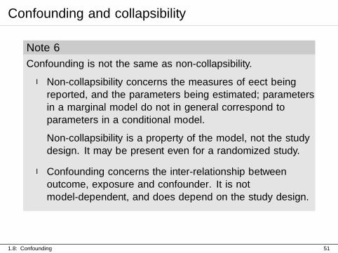
Confounding is not the same as non-collapsibility.
I Non-collapsibility concerns the measures of effect beingreported, and the parameters being estimated; parametersin a marginal model do not in general correspond toparameters in a conditional model.
Non-collapsibility is a property of the model, not the studydesign. It may be present even for a randomized study.
I Confounding concerns the inter-relationship betweenoutcome, exposure and confounder. It is notmodel-dependent, and does depend on the study design.
1.8: Confounding 51
Simple confounding example
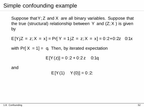
Suppose that Y, Z and X are all binary variables. Suppose thatthe true (structural) relationship between Y and (Z,X) is givenby
E[Y |Z = z,X = x] = Pr[Y = 1|Z = z,X = x] = 0.2+0.2z−0.1x
with Pr[X = 1] = q. Then, by iterated expectation
E[Y (z)] = 0.2 + 0.2 z − 0.1q
andE[Y (1)− Y (0)] = 0.2.
1.8: Confounding 52
Simple confounding example
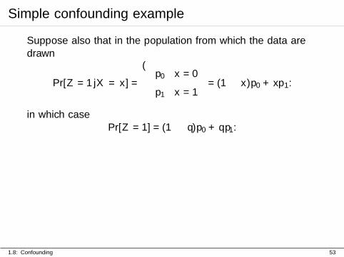
Suppose also that in the population from which the data aredrawn
Pr[Z = 1|X = x] =
{p0 x = 0
p1 x = 1= (1− x)p0 + xp1.
in which casePr[Z = 1] = (1− q)p0 + qp1.
1.8: Confounding 53
Simple confounding example
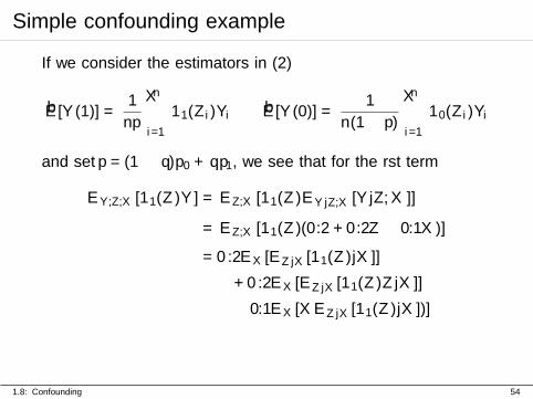
If we consider the estimators in (2)
E[Y (1)] =1
np
n∑i=1
11(Zi)Yi E[Y (0)] =1
n(1− p)
n∑i=1
10(Zi)Yi
and set p = (1− q)p0 + qp1, we see that for the first term
EY,Z,X [11(Z)Y ] = EZ,X [11(Z)EY |Z,X [Y |Z,X]]
= EZ,X [11(Z)(0.2 + 0.2Z − 0.1X)]
= 0.2EX [EZ|X [11(Z)|X]]
+ 0.2EX [EZ|X [11(Z)Z|X]]
− 0.1EX [XEZ|X [11(Z)|X])]
1.8: Confounding 54
Simple confounding example
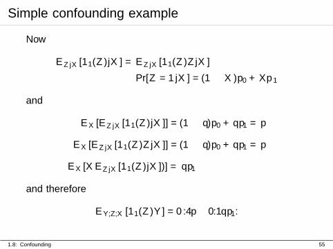
Now
EZ|X [11(Z)|X] = EZ|X [11(Z)Z|X]
≡ Pr[Z = 1|X] = (1−X)p0 +Xp1
and
EX [EZ|X [11(Z)|X]] = (1− q)p0 + qp1 = p
EX [EZ|X [11(Z)Z|X]] = (1− q)p0 + qp1 = p
EX [XEZ|X [11(Z)|X])] = qp1
and therefore
EY,Z,X [11(Z)Y ] = 0.4p− 0.1qp1.
1.8: Confounding 55
Simple confounding example
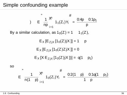
∴ E
[1
np
n∑i=1
11(Zi)Yi
]=
0.4p− 0.1p1p
By a similar calculation, as 10(Z) = 1− 11(Z),
EX [EZ|X [10(Z)|X]] = 1− p
EX [EZ|X [10(Z)Z|X]] = 0
EX [XEZ|X [10(Z)|X])] = q(1− p1)
so
E
[1
n(1− p)
n∑i=1
10(Zi)Yi
]=
0.2(1− p)− 0.1q(1− p1)1− p
1.8: Confounding 56
Simple confounding example
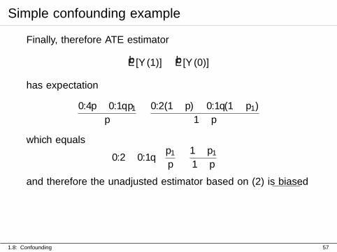
Finally, therefore ATE estimator
E[Y (1)]− E[Y (0)]
has expectation
0.4p− 0.1qp1p
− 0.2(1− p)− 0.1q(1− p1)1− p
which equals
0.2− 0.1q
{p1p− 1− p1
1− p
}and therefore the unadjusted estimator based on (2) is biased.
1.8: Confounding 57
Simple confounding example
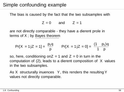
The bias is caused by the fact that the two subsamples with
Z = 0 and Z = 1
are not directly comparable - they have a different profile interms of X; by Bayes theorem
Pr[X = 1|Z = 1] =p1q
pPr[X = 1|Z = 0] =
(1− p1)q1− p
so, here, conditioning on Z = 1 and Z = 0 in turn in thecomputation of (2), leads to a different composition of X valuesin the two subsamples.
As X structurally influences Y , this renders the resulting Yvalues not directly comparable.
1.8: Confounding 58
Instruments
If predictor Z predicts Z, but does not predict Y in thepresence of Z, then Z is termed an instrument.
Example: Non-compliance
In a randomized study of a binary treatment, if Zi records thetreatment actually received by individual i, suppose that thereis non-compliance with respect to the treatment; that is, if Zirecords the treatment assigned by the experimenter, thenpossibly
zi 6= zi.
Then Zi predicts Zi, but is not associated with outcome Yigiven Zi.
1.8: Confounding 59
Instruments
Instruments are not confounders as they do not predict outcomeonce the influence of the exposure has been accounted for.
Suppose in the previous confounding example, we had
E[Y |Z = z,X = 0] = Pr[Y = 1|Z = z,X = 1] = 0.2 + 0.2z
for the structural model, but
Pr[Z = 1|X] = (1−X)p0 +Xp1.
Then X influences Z, and there is still an imbalance in the twosubgroups indexed by Z with respect to the X values, but as Xdoes not influence Y , there is no bias if the ATE estimatorbased on (2) is used.
1.8: Confounding 60
Critical Assumption
An important assumption that is commonly made is that of
No unmeasured confounding
that is, the measured predictors X include (possibly as asubset) all variables that confound the effect of Z on Y .
We must assume that all variables that simultaneously influenceexposure and outcome have been measured in the study.
This is a strong (and possibly unrealistic) assumption inpractical applications. It may be relaxed and the influence ofunmeasured confounders studied in sensitivity analyses.
1.8: Confounding 61
Model-based analysis
So far, estimation based on the data via (1) and (2) hasproceeded in a nonparametric or model-free fashion.
I models such asfY (z),X(y, x)
have been considered, but not modelled parametrically.
We now consider semiparametric specifications, specificallymodels where parametric models for example for
E[Y (z)|X]
are considered.
1.9: Statistical modelling 62
Correct model specification
Suppose we posit an outcome conditional mean model
E[Y |Z,X] = µ(Z,X)
that may be parametric in nature, say
E[Y |Z,X;β] = µ(Z,X;β)
which perhaps might be linear in β, or a monotone transform ofa linear function of β.
1.9: Statistical modelling 63
The importance of ‘no unmeasured confounders’
An important consequence of the no unmeasured confoundersassumption is that we have the equivalence of the conditionalmean structural and observed-data outcome models, that is
E[Y (z)|X] and E[Y |X,Z = z]
when this model is correctly specified.
1.9: Statistical modelling 64
Inference under correct specification
We might (optimistically) assume that the model E[Y |Z,X] iscorrectly specified, and captures the true relationship.
If this is, in fact, the case, then
No special (causal) techniques are needed to estimatethe causal effect.
That is, we may simply use regression of Y on (Z,X) usingmean model E[Y |Z,X].
1.9: Statistical modelling 65
Inference under correct specification
To estimate the APO, we simply set
E[Y (z)] =1
n
n∑i=1
µ(z, Xi) (3)
and derive other estimates from this: if µ(z, x) correctlycaptures the relationship of the outcome to the exposure andconfounders, then the estimator in (3) is consistent.
1.9: Statistical modelling 66
Inference under correct specification
The third challenge of causal inference is that
correct specification cannot be guaranteed.
I we may not capture the relationship between Y and (Z,X)correctly.
1.9: Statistical modelling 67

Part 2
The Propensity Score
68
Constructing a balanced sample
Recall the randomized trial setting in the case of a binaryexposure.
I we obtain a random sample of size n of individuals fromthe target population, and measure their X values;
I according to some random assignment procedure, weintervene to assign treatment Z to individuals, andmeasure their outcome Y ;
I the link between X and Z is broken by the randomallocation.
2.1: Manufacturing balance 69
Constructing a balanced sample
Recall that this procedure led to the valid use of the estimatorsof the ATE based on (1) and (2).
The important feature of the randomized study is that we have,for confounders X (indeed all predictors)
fX|Z(x|1) ≡ fX|Z(x|0) for all x,
or equivalently, in the case of a binary confounder,
Pr[X = 1|Z = 1] = Pr[X = 1|Z = 0].
2.1: Manufacturing balance 70
Constructing a balanced sample
The distribution of X is balanced across the two exposuregroups; this renders direct comparison of the outcomes possible.Probabilistically, X and Z are independent.
In a non-randomized study, there is a possibility that the twoexposure groups are not balanced
fX|Z(x|1) 6= fX|Z(x|0) for some x,
or in the binary case
Pr[X = 1|Z = 1] 6= Pr[X = 1|Z = 0].
If X influences Y also, then this imbalance renders directcomparison of outcomes in the two groups impossible.
2.1: Manufacturing balance 71
Constructing a balanced sample
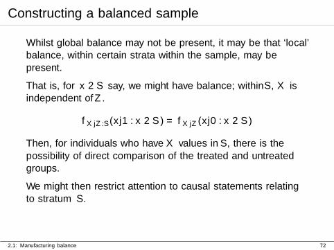
Whilst global balance may not be present, it may be that ‘local’balance, within certain strata within the sample, may bepresent.
That is, for x ∈ S say, we might have balance; within S, X isindependent of Z.
fX|Z:S(x|1 : x ∈ S) = fX|Z(x|0 : x ∈ S)
Then, for individuals who have X values in S, there is thepossibility of direct comparison of the treated and untreatedgroups.
We might then restrict attention to causal statements relatingto stratum S.
2.1: Manufacturing balance 72
Constructing a balanced sample
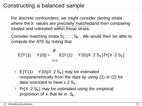
For discrete confounders, we might consider defining stratawhere the X values are precisely matched, and then comparingtreated and untreated within those strata.
Consider matching strata S1, . . . ,SK . We would then be able tocompute the ATE by noting that
E[Y (1)− Y (0)] =
K∑k=1
E[Y (1)− Y (0)|X ∈ Sk] Pr[X ∈ Sk]
I E[Y (1)− Y (0)|X ∈ Sk] may be estimatednonparametrically from the data by using (1) or (2) fordata restricted to have x ∈ Sk.
I Pr[X ∈ Sk] may be estimated using the empiricalproportion of x that lie in Sk.
2.1: Manufacturing balance 73
Constructing a balanced sample
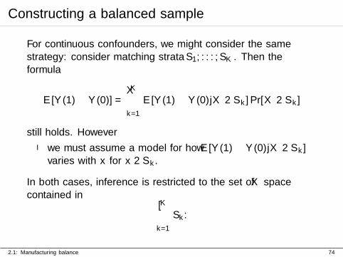
For continuous confounders, we might consider the samestrategy: consider matching strata S1, . . . ,SK . Then theformula
E[Y (1)− Y (0)] =
K∑k=1
E[Y (1)− Y (0)|X ∈ Sk] Pr[X ∈ Sk]
still holds. However
I we must assume a model for how E[Y (1)− Y (0)|X ∈ Sk]varies with x for x ∈ Sk.
In both cases, inference is restricted to the set of X spacecontained in
K⋃k=1
Sk.
2.1: Manufacturing balance 74
Constructing a balanced sample
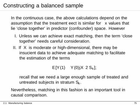
In the continuous case, the above calculations depend on theassumption that the treatment effect is similar for x values thatlie ‘close together’ in predictor (confounder) space. However
I. Unless we can achieve exact matching, then the term ‘closetogether’ needs careful consideration.
II. If X is moderate or high-dimensional, there may beinsufficient data to achieve adequate matching to facilitatethe estimation of the terms
E[Y (1)− Y (0)|X ∈ Sk];
recall that we need a large enough sample of treated anduntreated subjects in stratum Sk.
Nevertheless, matching in this fashion is an important tool incausal comparison.
2.1: Manufacturing balance 75
Balance via the propensity score
We now introduce the important concept of the propensity scorethat facilitates causal comparison via a balancing approach.
Recall that our goal is to mimic the construction of therandomized study that facilitates direct comparison betweentreated and untreated groups. We may not be able to achievethis globally, but possibly can achieve it locally in strata of Xspace.
The question is how to define these strata.
2.2: The propensity score for binary exposures 76
Balance via the propensity score
Recall that in the binary exposure case, balance corresponds tobeing able to state that within S, X is independent of Z:
fX|Z:S(x|1 : x ∈ S) = fX|Z(x|0 : x ∈ S)
This can be achieved if S is defined in terms of a statistic, e(X)say. That is, we consider the conditional distribution
fX|Z,e(X)(x|z, e)
and attempt to ensure that, given e(X) = e, Z is independentof X, so that within strata of e(X), the treated and untreatedgroups are directly comparable.
2.2: The propensity score for binary exposures 77
Balance via the propensity score
By Bayes theorem, for z = 0, 1, we have that
fX|Z,e(X)(x|z, e) =fZ|X,e(X)(z|x, e)fX|e(X)(x|e)
fZ|e(X)(z|e)(4)
Now, as Z is binary, we must be able to write the density in thedenominator as
fZ|e(X)(z|e) = p(e)z(1− p(e))1−z z ∈ 0, 1
where p(e) is a probability, a function of the fixed value e, andwhere p(e) > 0.
2.2: The propensity score for binary exposures 78
Balance via the propensity score
Therefore, in order to make the density fX|Z,e(X)(x|z, e)functionally independent of z, and achieve the necessaryindependence, we must have that
fZ|X,e(X)(z|x, e) = p(e)z(1− p(e))1−z z ∈ 0, 1
also. But e(X) is a function of X, so automatically we have that
fZ|X,e(X)(z|x, e) ≡ fZ|X(z|x).
Therefore, we require that
fZ|X(z|x) = fZ|X(z|x, e) = p(e)z(1− p(e))1−z ≡ fZ|e(X)(z|e)
for all relevant z, x.
2.2: The propensity score for binary exposures 79
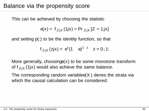
Balance via the propensity score
This can be achieved by choosing the statistic
e(x) = fZ|X(1|x) = PrZ|X [Z = 1|x]
and setting p(.) to be the identity function, so that
fZ|X(z|x) = ez(1− e)1−z z = 0, 1.
More generally, choosing e(x) to be some monotone transformof fZ|X(1|x) would also achieve the same balance.
The corresponding random variable e(X) defines the strata viawhich the causal calculation can be considered.
2.2: The propensity score for binary exposures 80
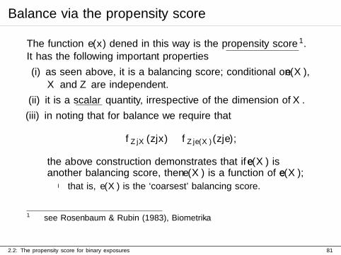
Balance via the propensity score
The function e(x) defined in this way is the propensity score1.It has the following important properties
(i) as seen above, it is a balancing score; conditional on e(X),X and Z are independent.
(ii) it is a scalar quantity, irrespective of the dimension of X.
(iii) in noting that for balance we require that
fZ|X(z|x) ≡ fZ|e(X)(z|e),
the above construction demonstrates that if e(X) isanother balancing score, then e(X) is a function of e(X);
I that is, e(X) is the ‘coarsest’ balancing score.
1 see Rosenbaum & Rubin (1983), Biometrika
2.2: The propensity score for binary exposures 81
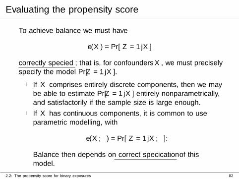
Evaluating the propensity score
To achieve balance we must have
e(X) = Pr[Z = 1|X]
correctly specified; that is, for confounders X, we must preciselyspecify the model Pr[Z = 1|X].
I If X comprises entirely discrete components, then we maybe able to estimate Pr[Z = 1|X] entirely nonparametrically,and satisfactorily if the sample size is large enough.
I If X has continuous components, it is common to useparametric modelling, with
e(X;α) = Pr[Z = 1|X;α].
Balance then depends on correct specification of thismodel.
2.2: The propensity score for binary exposures 82
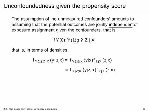
Unconfoundedness given the propensity score
The assumption of ‘no unmeasured confounders’ amounts toassuming that the potential outcomes are jointly independent ofexposure assignment given the confounders, that is
{Y (0), Y (1)} ⊥ Z |X
that is, in terms of densities
fY (z),Z|X(y, z|x) = fY (z)|X(y|x)fZ|X(z|x)
= fY |Z,X(y|z, x)fZ|X(z|x).
2.2: The propensity score for binary exposures 83
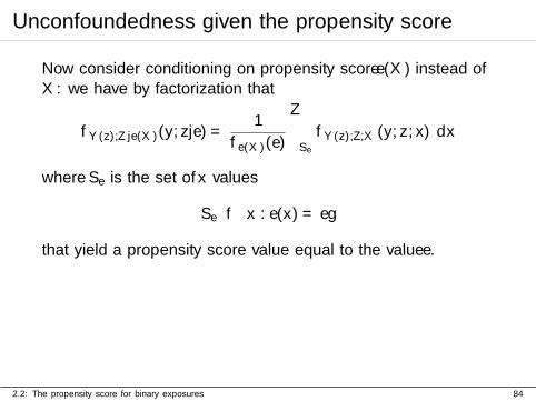
Unconfoundedness given the propensity score
Now consider conditioning on propensity score e(X) instead ofX: we have by factorization that
fY (z),Z|e(X)(y, z|e) =1
fe(X)(e)
∫SefY (z),Z,X(y, z, x) dx
where Se is the set of x values
Se ≡ {x : e(x) = e}
that yield a propensity score value equal to the value e.
2.2: The propensity score for binary exposures 84
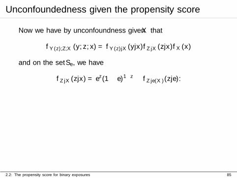
Unconfoundedness given the propensity score
Now we have by unconfoundness given X that
fY (z),Z,X(y, z, x) = fY (z)|X(y|x)fZ|X(z|x)fX(x)
and on the set Se, we have
fZ|X(z|x) = ez(1− e)1−z ≡ fZ|e(X)(z|e).
2.2: The propensity score for binary exposures 85
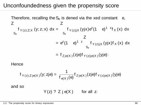
Unconfoundedness given the propensity score
Therefore, recalling the Se is defined via the fixed constant e,∫SefY (z),Z,X(y, z, x) dx =
∫SefY (z)|X(y|x)ez(1− e)1−zfX(x) dx
= ez(1− e)1−z∫SefY (z)|X(y|x)fX(x) dx
= fZ|e(X)(z|e)fY (z)|e(X)(y|e).
Hence
fY (z),Z|e(X)(y, z|e) =1
fe(X)(e)fZ|e(X)(z|e)fY (z)|e(X)(y|e)
and soY (z) ⊥ Z | e(X) for all z.
2.2: The propensity score for binary exposures 86
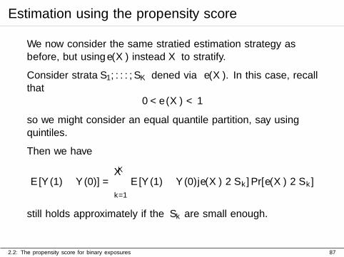
Estimation using the propensity score
We now consider the same stratified estimation strategy asbefore, but using e(X) instead X to stratify.
Consider strata S1, . . . ,SK defined via e(X). In this case, recallthat
0 < e(X) < 1
so we might consider an equal quantile partition, say usingquintiles.
Then we have
E[Y (1)− Y (0)] =
K∑k=1
E[Y (1)− Y (0)|e(X) ∈ Sk] Pr[e(X) ∈ Sk]
still holds approximately if the Sk are small enough.
2.2: The propensity score for binary exposures 87
Estimation using the propensity score
This still requires us to be able to estimate
E[Y (1)− Y (0)|e(X) ∈ Sk]
which requires us to have a sufficient number of treated anduntreated individuals with e(X) ∈ Sk to facilitate the ‘directcomparison’ within this stratum.
If the expected responses are constant across the stratum, theformulae (1) and (2) may be used.
2.2: The propensity score for binary exposures 88
Matching
The derivation of the propensity score indicates that it may beused to construct matched individuals or groups that can becompared directly.
I if two individuals have precisely the same value of e(x),then they are exactly matched;
I if one of the pair is treated and the other untreated, thentheir outcomes can be compared directly, as any imbalancebetween their measured confounder values has beenremoved by the fact that they are matched on e(x);
I this is conceptually identical to the standard procedure ofmatching in two-group comparison.
2.3: Matching via the propensity score 89
Matching
For an exactly matched pair (i1, i0), treated and untreatedrespectively, the quantity
yi1 − yi0
is an unbiased estimate of the ATE
E[Y (1)− Y (0)];
more typically we might choose m such matched pairs, usuallywith different e(x) values across pairs, and use the estimate
1
m
m∑i=1
(yi1 − yi0)
2.3: Matching via the propensity score 90

Matching
Exact matching is difficult to achieve, therefore we morecommonly attempt to achieve approximate matching
I May match one treated to M untreated (1 : M matching)
I caliper matching;
I nearest neighbour/kernel matching;
I matching with replacement.
Most standard software packages have functions that provideautomatic matching using a variety of methods.
2.3: Matching via the propensity score 91
Beyond binary exposures
The theory developed above extends beyond the case of binaryexposures.
Recall that we require balance to proceed with causalcomparisons; essentially, with strata defined using X or e(X),the distribution of X should not depend on Z.
We seek a scalar statistic such that, conditional on the value ofthat statistic, X and Z are independent. In the case of generalexposures, we must consider balancing scores that are functionsof both Z and X.
2.4: The Generalized Propensity Score 92
Beyond binary exposures
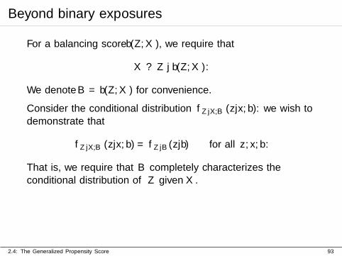
For a balancing score b(Z,X), we require that
X ⊥ Z | b(Z,X).
We denote B = b(Z,X) for convenience.
Consider the conditional distribution fZ|X,B(z|x, b): we wish todemonstrate that
fZ|X,B(z|x, b) = fZ|B(z|b) for all z, x, b.
That is, we require that B completely characterizes theconditional distribution of Z given X.
2.4: The Generalized Propensity Score 93
Beyond binary exposures
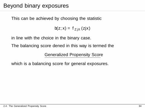
This can be achieved by choosing the statistic
b(z, x) = fZ|X(z|x)
in line with the choice in the binary case.
The balancing score defined in this way is termed the
Generalized Propensity Score
which is a balancing score for general exposures.
2.4: The Generalized Propensity Score 94
Beyond binary exposures
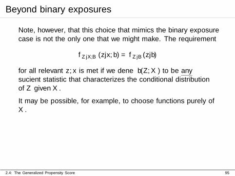
Note, however, that this choice that mimics the binary exposurecase is not the only one that we might make. The requirement
fZ|X,B(z|x, b) = fZ|B(z|b)
for all relevant z, x is met if we define b(Z,X) to be anysufficient statistic that characterizes the conditional distributionof Z given X.
It may be possible, for example, to choose functions purely ofX.
2.4: The Generalized Propensity Score 95
Beyond binary exposures
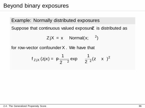
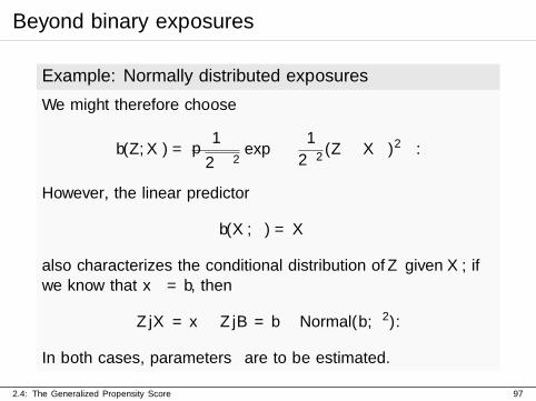
Example: Normally distributed exposures
Suppose that continuous valued exposure Z is distributed as
Z|X = x ∼ Normal(xα, σ2)
for row-vector confounder X. We have that
fZ|X(z|x) =1√
2πσ2exp
{− 1
2σ2(z − xα)2
}
2.4: The Generalized Propensity Score 96
Beyond binary exposures
Example: Normally distributed exposures
We might therefore choose
b(Z,X) =1√
2πσ2exp
{− 1
2σ2(Z −Xα)2
}.
However, the linear predictor
b(X;α) = Xα
also characterizes the conditional distribution of Z given X; ifwe know that xα = b, then
Z|X = x ≡ Z|B = b ∼ Normal(b, σ2).
In both cases, parameters α are to be estimated.
2.4: The Generalized Propensity Score 97
Beyond binary exposures
The generalized propensity score inherits all the properties ofthe standard propensity score;
I it induces balance;
I if the potential outcomes and exposure are independentgiven X under the unconfoundeness assumption, they arealso independent given b(Z,X).
However, how exactly to use the generalized propensity score incausal adjustment for continuous exposures is not clear.
2.4: The Generalized Propensity Score 98
Propensity Score Regression
Up to this point we have considered using the propensity scorefor stratification, that is, to produce directly comparable groupsof treated and untreated individuals.
Causal comparison can also be carried out using regressiontechniques: that is, we consider building an estimator of theAPO by regressing the outcome on a function of the exposureand the propensity score.
Regressing on the propensity score is a means of controlling theconfounding.
2.5: Propensity score regression 99
Propensity Score Regression
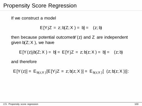
If we construct a model
E[Y |Z = z, b(Z,X) = b] = µ(z, b)
then because potential outcomes Y (z) and Z are independentgiven b(Z,X), we have
E[Y (z)|b(Z,X) = b] = E[Y |Z = z, b(z, X) = b] = µ(z, b)
and therefore
E[Y (z)] = Eb(z,X)[E[Y |Z = z, b(z, X)] = Eb(z,X)[µ(z, b(z, X))].
2.5: Propensity score regression 100
Propensity Score Regression
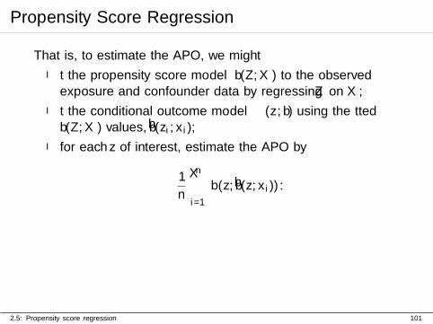
That is, to estimate the APO, we might
I fit the propensity score model b(Z,X) to the observedexposure and confounder data by regressing Z on X;
I fit the conditional outcome model µ(z, b) using the fittedb(Z,X) values, b(zi, xi);
I for each z of interest, estimate the APO by
1
n
n∑i=1
µ(z, b(z, xi)).
2.5: Propensity score regression 101
Propensity Score Regression
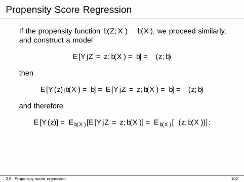
If the propensity function b(Z,X) ≡ b(X), we proceed similarly,and construct a model
E[Y |Z = z, b(X) = b] = µ(z, b)
then
E[Y (z)|b(X) = b] = E[Y |Z = z, b(X) = b] = µ(z, b)
and therefore
E[Y (z)] = Eb(X)[E[Y |Z = z, b(X)] = Eb(X)[µ(z, b(X))].
2.5: Propensity score regression 102
Propensity Score Regression
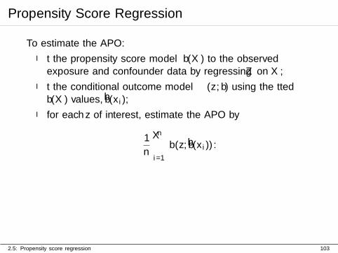
To estimate the APO:
I fit the propensity score model b(X) to the observedexposure and confounder data by regressing Z on X;
I fit the conditional outcome model µ(z, b) using the fittedb(X) values, b(xi);
I for each z of interest, estimate the APO by
1
n
n∑i=1
µ(z, b(xi)).
2.5: Propensity score regression 103
Example: Binary Exposure
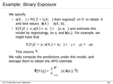
We specify
I e(X;α) = Pr[Z = 1|X,α] then regress Z on X to obtain αand fitted values e(X) ≡ e(X; α).
I E[Y |Z = z, e(X) = e;β] = µ(z, e;β) and estimate thismodel by regressing yi on zi and e(xi). For example, wemight have that
E[Y |Z = zi, e(Xi) = ei;β] = β0 + β1zi + β2ei.
This returns β.
We finally compute the predictions under this model, andaverage them to obtain the APO estimate
E[Y (z)] =1
n
n∑i=1
µ(z, e(xi); β).
2.5: Propensity score regression 104
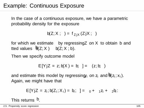
Example: Continuous Exposure
In the case of a continuous exposure, we have a parametricprobability density for the exposure
b(Z,X;α) = fZ|X(Z|X;α)
for which we estimate α by regressing Z on X to obtain α andfitted values b(Z,X) ≡ b(Z,X; α).
Then we specify outcome model
E[Y |Z = z, b(X) = b;β] = µ(z, b;β)
and estimate this model by regressing yi on zi and b(zi, xi).Again, we might have that
E[Y |Z = zi, b(Zi, Xi) = bi;β] = β0 + β1zi + β2bi.
This returns β.2.5: Propensity score regression 105
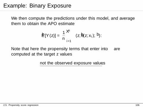
Example: Binary Exposure
We then compute the predictions under this model, and averagethem to obtain the APO estimate
E[Y (z)] =1
n
n∑i=1
µ(z, b(z, xi); β).
Note that here the propensity terms that enter into µ arecomputed at the target z values
not the observed exposure values.
2.5: Propensity score regression 106
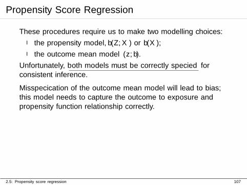
Propensity Score Regression
These procedures require us to make two modelling choices:
I the propensity model, b(Z,X) or b(X);
I the outcome mean model µ(z, b).
Unfortunately, both models must be correctly specified forconsistent inference.
Misspecification of the outcome mean model will lead to bias;this model needs to capture the outcome to exposure andpropensity function relationship correctly.
2.5: Propensity score regression 107

Weighting approaches
For a causal quantity of interest, we focus on he APO
E[Y (z)] =
∫y fY (z),X(y, x) dy dx
that is, the average outcome, over the distribution of theconfounders and predictors, if we hypothesize that theintervention sets the exposure to z.
We now study methods that utilize the components alreadydescribed, including the propensity score, but in a differentfashion;
I instead of accounting for confounding by balancing throughmatching, we aim to achieve balance via weighting
2.6: Adjustment by weighting 108
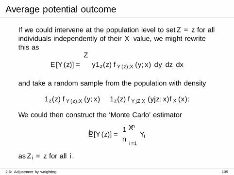
Average potential outcome
If we could intervene at the population level to set Z = z for allindividuals independently of their X value, we might rewritethis as
E[Y (z)] =
∫y1z(z) fY (z),X(y, x) dy dz dx
and take a random sample from the population with density
1z(z) fY (z),X(y, x) ≡ 1z(z) fY |Z,X(y|z, x)fX(x).
We could then construct the ‘Monte Carlo’ estimator
E[Y (z)] =1
n
n∑i=1
Yi
as Zi = z for all i.
2.6: Adjustment by weighting 109
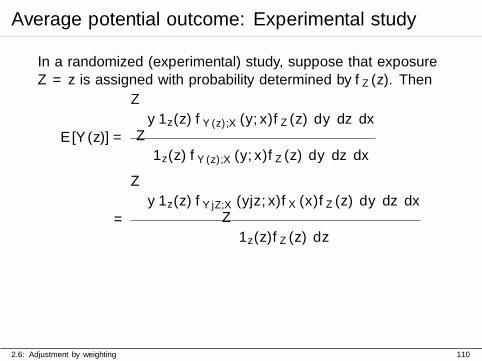
Average potential outcome: Experimental study
In a randomized (experimental) study, suppose that exposureZ = z is assigned with probability determined by fZ(z). Then
E[Y (z)] =
∫y 1z(z) fY (z),X(y, x)fZ(z) dy dz dx∫1z(z) fY (z),X(y, x)fZ(z) dy dz dx
=
∫y 1z(z) fY |Z,X(y|z, x)fX(x)fZ(z) dy dz dx∫
1z(z)fZ(z) dz
2.6: Adjustment by weighting 110
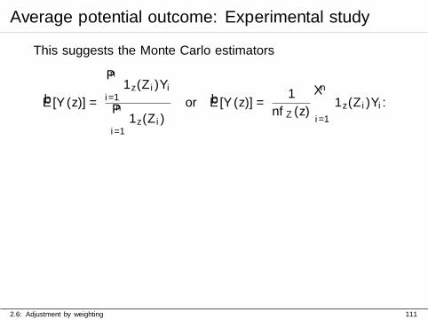
Average potential outcome: Experimental study
This suggests the Monte Carlo estimators
E[Y (z)] =
n∑i=1
1z(Zi)Yi
n∑i=1
1z(Zi)
or E[Y (z)] =1
nfZ(z)
n∑i=1
1z(Zi)Yi.
2.6: Adjustment by weighting 111
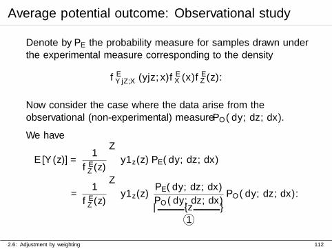
Average potential outcome: Observational study
Denote by PE the probability measure for samples drawn underthe experimental measure corresponding to the density
fEY |Z,X(y|z, x)fEX(x)fEZ(z).
Now consider the case where the data arise from theobservational (non-experimental) measure PO( dy, dz, dx).
We have
E[Y (z)] =1
fEZ(z)
∫y1z(z) PE( dy, dz, dx)
=1
fEZ(z)
∫y1z(z)
PE( dy, dz, dx)
PO( dy, dz, dx)︸ ︷︷ ︸1
PO( dy, dz, dx).
2.6: Adjustment by weighting 112
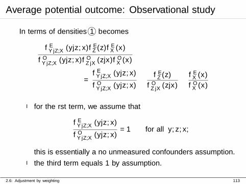
Average potential outcome: Observational study
In terms of densities 1 becomes
fEY |Z,X(y|z, x)fEZ(z)fEX(x)
fOY |Z,X(y|z, x)fOZ|X(z|x)fOX (x)
=fEY |Z,X(y|z, x)
fOY |Z,X(y|z, x)×
fEZ(z)
fOZ|X(z|x)×fEX(x)
fOX (x)
I for the first term, we assume that
fEY |Z,X(y|z, x)
fOY |Z,X(y|z, x)= 1 for all y, z, x;
this is essentially a no unmeasured confounders assumption.
I the third term equals 1 by assumption.
2.6: Adjustment by weighting 113
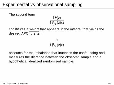
Experimental vs observational sampling
The second termfEZ(z)
fOZ|X(z|x)
constitutes a weight that appears in the integral that yields thedesired APO; the term
1
fOZ|X(z|x)
accounts for the imbalance that influences the confounding andmeasures the difference between the observed sample and ahypothetical idealized randomized sample.
2.6: Adjustment by weighting 114

Estimation
This suggests the (nonparametric) estimators
E[Y (z)] =1
n
n∑i=1
1z(Zi)Yi
fOZ|X(Zi|Xi)(IPW0)
which is unbiased, or
E[Y (z)] =
n∑i=1
1z(Zi)Yi
fOZ|X(Zi|Xi)
n∑i=1
1z(Zi)
fOZ|X(Zi|Xi)
(IPW)
which is consistent, each provided fOZ|X(.|.) correctly specifies
the conditional density of Z given X for all (z, x).
2.6: Adjustment by weighting 115
Inverse weighting and the propensity score
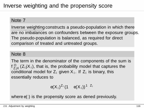
Note 7
Inverse weighting constructs a pseudo-population in which thereare no imbalances on confounders between the exposure groups.The pseudo-population is balanced, as required for directcomparison of treated and untreated groups.
Note 8
The term in the denominator of the components of the sum isfOZ|X(Zi|Xi), that is, the probability model that captures theconditional model for Zi given Xi. If Zi is binary, thisessentially reduces to
e(Xi)Zi(1− e(Xi))
1−Zi
where e(.) is the propensity score as defined previously.
2.6: Adjustment by weighting 116
Positivity
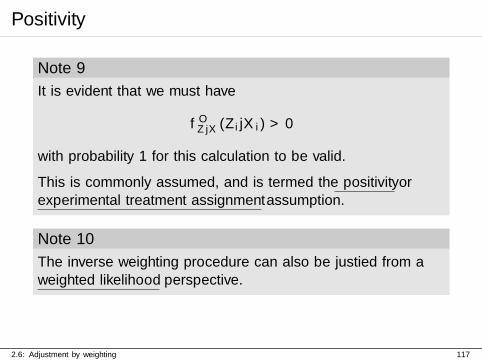
Note 9
It is evident that we must have
fOZ|X(Zi|Xi) > 0
with probability 1 for this calculation to be valid.
This is commonly assumed, and is termed the positivity orexperimental treatment assignment assumption.
Note 10
The inverse weighting procedure can also be justified from aweighted likelihood perspective.
2.6: Adjustment by weighting 117
Estimation via Augmentation
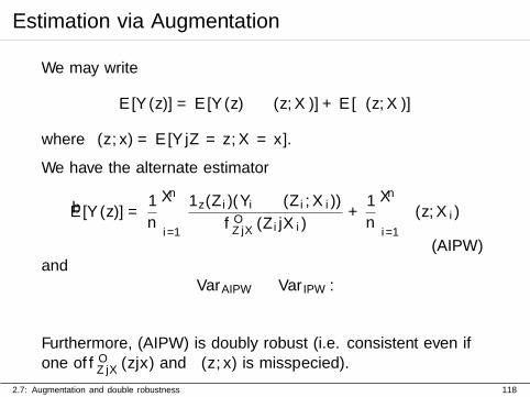
We may write
E[Y (z)] = E[Y (z)− µ(z, X)] +E[µ(z, X)]
where µ(z, x) = E[Y |Z = z,X = x].
We have the alternate estimator
E[Y (z)] =1
n
n∑i=1
1z(Zi)(Yi − µ(Zi, Xi))
fOZ|X(Zi|Xi)+
1
n
n∑i=1
µ(z, Xi)
(AIPW)and
VarAIPW ≤ VarIPW.
Furthermore, (AIPW) is doubly robust (i.e. consistent even ifone of fOZ|X(z|x) and µ(z, x) is misspecified).
2.7: Augmentation and double robustness 118
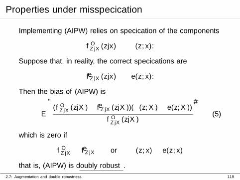
Properties under misspecification
Implementing (AIPW) relies on specification of the components
fOZ|X(z|x) µ(z, x).
Suppose that, in reality, the correct specifications are
fZ|X(z|x) µ(z, x).
Then the bias of (AIPW) is
E
[(fOZ|X(z|X)− fZ|X(z|X))(µ(z, X)− µ(z, X))
fOZ|X(z|X)
](5)
which is zero if
fOZ|X ≡ fZ|X or µ(z, x) ≡ µ(z, x)
that is, (AIPW) is doubly robust.
2.7: Augmentation and double robustness 119
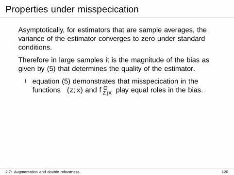
Properties under misspecification
Asymptotically, for estimators that are sample averages, thevariance of the estimator converges to zero under standardconditions.
Therefore in large samples it is the magnitude of the bias asgiven by (5) that determines the quality of the estimator.
I equation (5) demonstrates that misspecification in thefunctions µ(z, x) and fOZ|X play equal roles in the bias.
2.7: Augmentation and double robustness 120
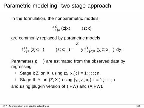
Parametric modelling: two-stage approach
In the formulation, the nonparametric models
fOZ|X(z|x) µ(z, x)
are commonly replaced by parametric models
fOZ|X(z|x;α) µ(z, x;β) =
∫y fOY |Z,X(y|z, x;β) dy.
Parameters (α, β) are estimated from the observed data byregressing
I Stage I: Z on X using (zi, xi), i = 1, . . . , n,
I Stage II: Y on (Z,X) using (yi, zi, xi), i = 1, . . . , n
and using plug-in version of (IPW) and (AIPW).
2.7: Augmentation and double robustness 121
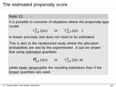
The estimated propensity score
Note 11
It is possible to conceive of situations where the propensity-typemodel
fOZ|X(z|x) or fOZ|X(z|x;α)
is known precisely and does not need to be estimated.
This is akin to the randomized study where the allocationprobabilities are fixed by the experimenter. It can be shownthat using estimated quantities
fOZ|X(z|x) or fOZ|X(z|x; α)
yields lower variances for the resulting estimators than if theknown quantities are used.
2.7: Augmentation and double robustness 122
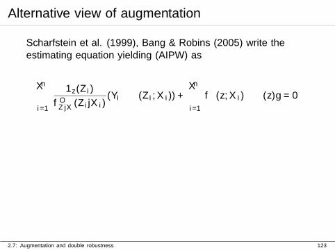
Alternative view of augmentation
Scharfstein et al. (1999), Bang & Robins (2005) write theestimating equation yielding (AIPW) as
n∑i=1
1z(Zi)
fOZ|X(Zi|Xi)(Yi − µ(Zi, Xi)) +
n∑i=1
{µ(z, Xi)− µ(z)} = 0
2.7: Augmentation and double robustness 123
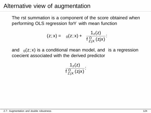
Alternative view of augmentation
The first summation is a component of the score obtained whenperforming OLS regression for Y with mean function
µ(z, x) = µ0(z, x) + ε1z(z)
fOZ|X(z|x).
and µ0(z, x) is a conditional mean model, and ε is a regressioncoefficient associated with the derived predictor
1z(z)
fOZ|X(z|x).
2.7: Augmentation and double robustness 124
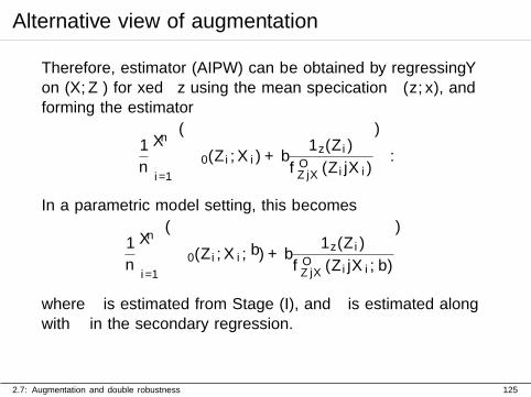
Alternative view of augmentation
Therefore, estimator (AIPW) can be obtained by regressing Yon (X,Z) for fixed z using the mean specification µ(z, x), andforming the estimator
1
n
n∑i=1
{µ0(Zi, Xi) + ε
1z(Zi)
fOZ|X(Zi|Xi)
}.
In a parametric model setting, this becomes
1
n
n∑i=1
{µ0(Zi, Xi; β) + ε
1z(Zi)
fOZ|X(Zi|Xi; α)
}
where α is estimated from Stage (I), and β is estimated alongwith ε in the secondary regression.
2.7: Augmentation and double robustness 125
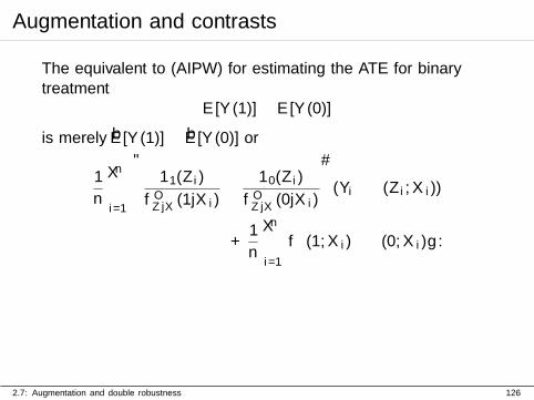
Augmentation and contrasts
The equivalent to (AIPW) for estimating the ATE for binarytreatment
E[Y (1)]−E[Y (0)]
is merely E[Y (1)]− E[Y (0)] or
1
n
n∑i=1
[11(Zi)
fOZ|X(1|Xi)− 10(Zi)
fOZ|X(0|Xi)
](Yi − µ(Zi, Xi))
+1
n
n∑i=1
{µ(1, Xi)− µ(0, Xi)} .
2.7: Augmentation and double robustness 126

Augmentation and contrasts
Therefore we can repeat the above argument and base thecontrast estimator on the regression of Y on (X,Z) using themean specification
µ(z, x) = µ0(z, x) + ε
[11(z)
fOZ|X(1|x)− 10(z)
fOZ|X(0|x)
]
2.7: Augmentation and double robustness 127

Part 3
Implementation and Computation
128
Statistical modelling tools
Causal inference typically relies on reasonably standardstatistical tools:
1. Standard distributions:
I Normal;I Binomial;I Time-to-event distributions (Exponential, Weibull etc.)
2. Regression tools:
I linear model/ordinary least squares;I generalized linear model, typically linear regression;I survival models.
3.1: Statistical tools 129
Pooled logistic regression
For a survival outcome, pooled logistic regression is often used.
The usual continuous survival time outcome is replaced by adiscrete, binary outcome;
I this is achieved by partitioning the outcome space intoshort intervals,
(0, t1], (t1, t2], . . .
and assuming that the failure density is approximatelyconstant in each interval.
I using a hazard parameterization, we have that
Pr[Failure in (tj−1, tj ]|No failure before tj−1] = qj
which converts each single failure time outcome into aseries of binary responses, with 0 recording ‘no failure’ and1 recording ‘failure’.
3.1: Statistical tools 130
Semiparametric estimation
Semiparametric models based on estimating equations aretypically used:
I such models make no parametric assumptions about thedistributions of the various quantities, but instead makemoment restrictions;
I resulting estimators inherit good asymptotic properties;
I variance of estimators typically estimated in a ‘robust’fashion using the sandwich estimator of the asymptoticvariance.
3.1: Statistical tools 131
Key considerations
In light of the previous discussions, in order to facilitate causalcomparisons, there are several key considerations thatpractitioners must take into account.
1. The importance of no unmeasured confounding.
When considering the study design, it is essential for validconclusions to have measured and recorded all confounders.
3.2: Key considerations 132
Key considerations
2. Model construction for the outcome regression.
I ideally, the model for the expected value of Y given Z andX, µ(z, x), should be correctly specified, that is, correctlycapture the relationship between outcome and the othervariables.
I if this can be done, then no causal adjustments arenecessary.
I conventional model building techniques (variable selection)can be used; this will prioritize predictors of outcome andtherefore will select all confounders;
I however, in finite sample, this method may omit weakconfounders that may lead to bias.
3.2: Key considerations 133
Key considerations
3. Model construction for the propensity score.Ideally, the model for the (generalized) propensity score,e(x) or b(z, x), should be correctly specified, that is,correctly capture the relationship between the exposureand the confounders. We focus on
3.1 identifying the confounders;3.2 ignoring the instruments: instruments do not predict the
outcome, therefore cannot be a source of bias (unless thereis unmeasured confounding) - however they can increase thevariability of the resulting propensity score estimators.
3.3 the need for the specified propensity model to inducebalance;
3.4 ensuring positivity, so that strata constructed from thepropensity score have sufficient data within them tofacilitate comparison;
3.5 effective model selection.
3.2: Key considerations 134
Key considerations
Note 12
Conventional model selection techniques (stepwise selection,selection via information criteria, sparse selection)should not be used when constructing the propensity score.
This is because such techniques prioritize the accurateprediction of exposure conditional on the other predictors;however, this is not the goal of the analysis.
These techniques may merely select strong instruments andomit strong predictors of outcome that are only weaklyassociated with exposure.
3.2: Key considerations 135
Key considerations
Note 13
An apparently conservative approach is to build rich (highlyparameterized) models for both µ(z, x) and e(x).
This approach prioritizes bias elimination at the cost ofvariance inflation.
3.2: Key considerations 136
Key considerations
4. The required measure of effect.Is the causal measure required
I a risk difference ?I a risk ratio ?I an odds ratio ?I an ATT, ATE or APO ?
3.2: Key considerations 137

Part 4
Extensions
138
Longitudinal studies
It is common for studies to involve multiple longitudinalmeasurements of exposure, confounders and outcomes.
In this case, the possible effect of confounding of the exposureeffect by the confounders is more complicated.
Furthermore, we may be interested in different types of effect:
I the direct effect: the effect of exposure in any given intervalon the outcome in that interval, or the final observedoutcome;
I the total effect: the effect of exposure aggregated acrossintervals final observed outcome;
4.1: Longitudinal studies 139

Illustration
Possible structure across five intervals:
X1//
��
��
X2//
��
��
X3//
��
��
X4//
��
��
X5
��
��
Z1//
((
Z2//
((
Z3//
((
Z4//
((
Z5
((Y1 //
@@
Y2 //
@@
Y3 //
@@
Y4 //
@@
Y5
4.1: Longitudinal studies 140
Mediation and time-varying confounding
I The effect of exposure on later outcomes may be mediatedthrough variables measured at intermediate time points
I for example, the effect of exposure Z1 may have a directeffect on Y1 that is confounded by X1; however, the effect ofZ1 on Y2 may also be non-negligible. This effect is mediatedvia X2.
I There may be time-varying confounding;
4.1: Longitudinal studies 141

Multivariate versions of the propensity score
The propensity score may be generalized to the multivariatesetting. We consider longitudinal versions of the measuredvariables: for j = 1, . . . ,m, consider
I exposure: Zij = (Zi1, . . . , Zij);
I outcome: Yij = (Yi1, . . . , Yij);
I confounders: Xij = (Xi1, . . . , Xij).
Sometimes the notation
Z1:m = (Z1, . . . , Zm)
will be useful.
4.1: Longitudinal studies 142
Multivariate versions of the propensity score
We consider vectors of potential outcomes corresponding tothese observed quantities, that is, we consider a potentialsequence of interventions up to time j
zij = (zi1, . . . , zij)
and then the corresponding sequence of potential outcomes
Y (zij) = (Y (zi1), . . . , Y (zij)).
4.1: Longitudinal studies 143
Multivariate versions of the propensity score
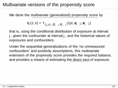
We define the multivariate (generalized) propensity score by
bj(z, x) = fZj |Xj ,Zj−1,Xj−1
(z|x, zj−1, xj−1)
that is, using the conditional distribution of exposure at intervalj, given the confounder at interval j, and the historical values ofexposures and confounders.
Under the sequential generalizations of the ‘no unmeasuredconfounders’ and positivity assumptions, this multivariateextension of the propensity score provides the required balance,and provides a means of estimating the direct effect of exposure.
4.1: Longitudinal studies 144
The use of mixed models
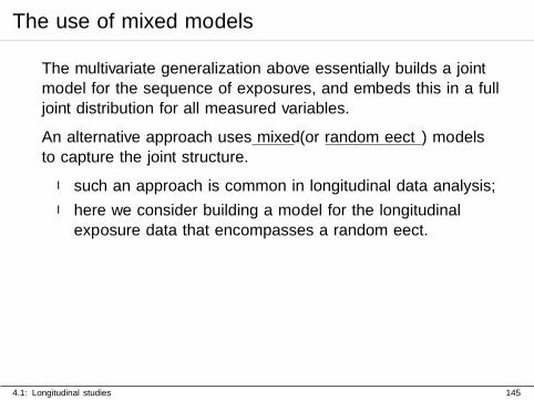
The multivariate generalization above essentially builds a jointmodel for the sequence of exposures, and embeds this in a fulljoint distribution for all measured variables.
An alternative approach uses mixed (or random effect) modelsto capture the joint structure.
I such an approach is common in longitudinal data analysis;
I here we consider building a model for the longitudinalexposure data that encompasses a random effect.
4.1: Longitudinal studies 145
The use of mixed models
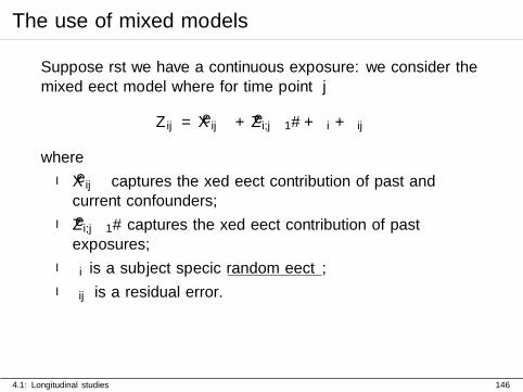
Suppose first we have a continuous exposure: we consider themixed effect model where for time point j
Zij = Xijα+ Zi,j−1ϑ+ ξi + εij
where
I Xijα captures the fixed effect contribution of past andcurrent confounders;
I Zi,j−1ϑ captures the fixed effect contribution of pastexposures;
I ξi is a subject specific random effect;
I εij is a residual error.
4.1: Longitudinal studies 146
The use of mixed models
The random effect ξi helps to capture unmeasuredtime-invariant confounding.
The distributional assumption made about εij determine theprecise form of a generalized propensity score that can again beused to estimate the direct effect of exposure.
4.1: Longitudinal studies 147
The use of mixed models
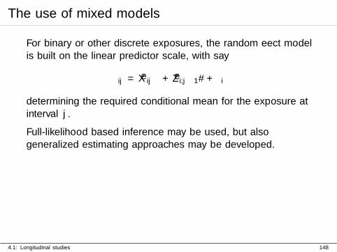
For binary or other discrete exposures, the random effect modelis built on the linear predictor scale, with say
ηij = Xijα+ Zi,j−1ϑ+ ξi
determining the required conditional mean for the exposure atinterval j.
Full-likelihood based inference may be used, but alsogeneralized estimating approaches may be developed.
4.1: Longitudinal studies 148
Estimation of Total Effects
The estimation of the total effect of exposure in longitudinalstudies is more complicated as the need to acknowledgemediation and time-varying confounding renders standardlikelihood-based approaches inappropriate.
The Marginal Structural Model is a semiparametric inverseweighting methodology designed to estimate total effects offunctions of aggregate exposures that generalizes conventionalinverse weighting.
4.2: The Marginal Structural Model (MSM) 149
The Marginal Structural Model
We observe for each individual i a sequence of exposures
Zi1, Zi2, . . . , Zim
and confoundersXi1, Xi2, . . . , Xim
along with outcome Yi ≡ Yim measured at the end of the study.
Intermediate outcomes Yi1, Yi2, . . . , Yi,m−1 also possiblyavailable.
We might also consider individual level frailty variables {υi},which are determinants of both the outcome and theintermediate variables, but can be assumed conditionallyindependent of the exposure assignments.
4.2: The Marginal Structural Model (MSM) 150
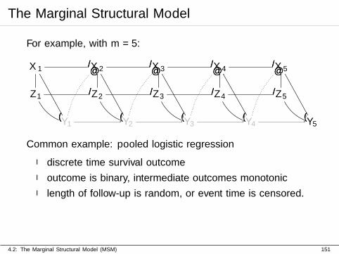
The Marginal Structural Model
For example, with m = 5:
X1//
��
��
X2//
��
��
X3//
��
��
X4//
��
��
X5
��
��
Z1//
((
Z2//
((
Z3//
((
Z4//
((
Z5
((Y1 //
@@
Y2 //
@@
Y3 //
@@
Y4 //
@@
Y5
Common example: pooled logistic regression
I discrete time survival outcome
I outcome is binary, intermediate outcomes monotonic
I length of follow-up is random, or event time is censored.
4.2: The Marginal Structural Model (MSM) 151
The Marginal Structural Model
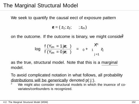
We seek to quantify the causal effect of exposure pattern
z = (z1, z2, · · · , zm)
on the outcome. If the outcome is binary, we might consider2
log
(f(Yim = 1|z, θ)f(Yim = 0|z, θ)
)= θ0 + θ1
m∑j=1
zj
as the true, structural model. Note that this is a marginalmodel.
To avoid complicated notation in what follows, all probabilitydistributions will be generically denoted p(.|.).2 We might also consider structural models in which the influence of co-
variates/confounders is recognized.
4.2: The Marginal Structural Model (MSM) 152
The Marginal Structural Model
However, this model is expressed for data presumed to becollected under an experimental design, E .
In reality, it is necessary to adjust for the influence of
I time-varying confounding due to the observational natureof exposure assignment
I mediation as past exposures may influence future values ofthe confounders, exposures and outcome.
The adjustment can be achieved using inverse weighting via amarginal structural model.
4.2: The Marginal Structural Model (MSM) 153
The Marginal Structural Model
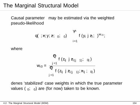
Causal parameter θ may be estimated via the weightedpseudo-likelihood
q(θ; x, y, z, γ0, α0) ≡n∏i=1
f(yi | zi, θ)wi0 ,
where
wi0 =
m∏j=1
f(zij | zi(j−1), α0j)
m∏j=1
f(zij | zi(j−1), xij , γ0j)
defines ‘stabilized’ case weights in which the true parametervalues (γ0, α0) are (for now) taken to be known.
4.2: The Marginal Structural Model (MSM) 154
The Marginal Structural Model: The logic
I Inference is required under target population E but asample from the population of interest is not directlyavailable
I Samples from observational design O relevant for learningabout this target population are available.
I In population E , the conditional independencezij ⊥ xij | zi(j−1) holds true.
I The weights wi0 convey information on how much Oresembles E : this information is contained in theparameters γ.
I E has the same marginal exposure assignment distributionas O, characterized by α.
4.2: The Marginal Structural Model (MSM) 155
The Marginal Structural Model: Implementation
I Parameters α typically must (and should) be estimatedfrom the exposure and confounder data;
I The usual logic of the propensity score applies here: inconstructing the terms that enter the conditional modelsthat enter into the stabilized weights, we use confoundersbut omit instruments.
I Inference using the weighted likelihood typically proceedsusing robust (sandwich) variance estimation, or thebootstrap.
4.2: The Marginal Structural Model (MSM) 156

Real Data Example : ART interruption in HIV/HCV co-infected individuals
Antiretroviral therapy (ART) has reduced morbidity andmortality due to nearly all HIV-related illnesses, apart frommortality due to end-stage liver disease, which has increasedsince ART treatment became widespread.
In part, this increase may be due to improved overall survivalcombined with Hepatitis C virus (HCV) associated hepatic liverfibrosis, the progress of which is accelerated by immunedysfunction related to HIV-infection.
4.2: The Marginal Structural Model (MSM) 157
Real Data Example : ART interruption in HIV/HCV co-infected individuals
The Canadian Co-infection Cohort Study is one of the largestprojects set up to study the role of ART on the development ofend-stage liver disease in HIV-HCV co-infected individuals.
Given the importance of ART in improving HIV-relatedimmunosuppression, it is hypothesized that liver fibrosisprogression in co-infected individuals may be partly related toadverse consequences of ART interruptions.
4.2: The Marginal Structural Model (MSM) 158
Real Data Example : ART interruption in HIV/HCV co-infected individuals
Study comprised N = 474 individuals with at least onefollow-up visit (scheduled at every six months) after thebaseline visit, and 2066 follow-up visits in total (1592 excludingthe baseline visits). The number of follow-up visits mi rangedfrom 2 to 16 (median 4).
4.2: The Marginal Structural Model (MSM) 159
Real Data Example : ART interruption in HIV/HCV co-infected individuals
We adopt a pooled logistic regression approach:
I a single binary outcome (death at study termination)
I longitudinal binary exposure (adherence to ART)
I possible confounders
I baseline covariates: female gender, hepatitis B surfaceantigen (HBsAg) test and baseline APRI, as well as
I time-varying covariates: age, current intravenous drug use(binary), current alcohol use (binary), duration of HCVinfection, HIV viral load, CD4 cell count, as well as ARTinterruption status at the previous visit.
I need also a model for informative censoring.
4.2: The Marginal Structural Model (MSM) 160
Real Data Example : ART interruption in HIV/HCV co-infected individuals
I We included co-infected adults who were not on HCVtreatment and did not have liver fibrosis at baseline.
I The outcome event was defined asaminotransferase-to-platelet ratio index (APRI), asurrogate marker for liver fibrosis, being at least 1.5 in anysubsequent visit
I We included visits where the individuals were either onART or had interrupted therapy (Zij = 1), based onself-reported medication information, during the 6 monthsbefore each follow-up visit.
4.2: The Marginal Structural Model (MSM) 161
Real Data Example : ART interruption in HIV/HCV co-infected individuals
I Individuals suspected of having spontaneously cleared theirHCV infection (based on two consecutive negative HCVviral load measurements) were excluded as they are notconsidered at risk for fibrosis progression.
I To ensure correct temporal order in the analyses, in thetreatment assignment model all time-varying covariates(xij), including the laboratory measurements (HIV viralload and CD4 cell count), were lagged one visit.
I Follow-up was terminated at the outcome event (Yij = 1),while individuals starting HCV medication during thefollow-up were censored.
4.2: The Marginal Structural Model (MSM) 162
Real Data Example : ART interruption in HIV/HCV co-infected individuals
We considered the structural model
log
(f(Yij = 1|zij , θ)f(Yij = 0|zij , θ)
)= θ0 + θ1zj
so that θ1 measures the total effect of exposure in an interval,allowing for mediation.
4.2: The Marginal Structural Model (MSM) 163
Real Data Example : ART interruption in HIV/HCV co-infected individuals
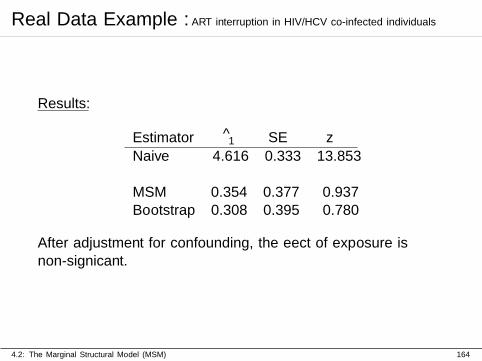
Results:
Estimator θ1 SE z
Naive 4.616 0.333 13.853
MSM 0.354 0.377 0.937Bootstrap 0.308 0.395 0.780
After adjustment for confounding, the effect of exposure isnon-significant.
4.2: The Marginal Structural Model (MSM) 164

Part 5
New Challenges and Approaches
165
New challenges
The main challenge for causal adjustments using the propensityscore is the nature of the observational data being recorded.
The data sets and databases being collected are increasinglycomplex and typically originate from different sources. Thebenefits of ‘Big Data’ come with the costs of more involvedcomputation and modelling.
There is always an important trade off between the sample sizen and the dimension of the confounder (and predictor) set.Examples
I pharmacoepidemiology;
I electronic health records and primary care decision making;
I real-time health monitoring;
5.1: New challenges 166
Data synthesis and combination
For observational databases, the choice of inclusion/exclusioncriteria for analysis can have profound influence on the ultimateresults:
I different databases can lead to different conclusions for thesame effect of interest purely because of the methodologyused to construct the raw data, irrespective of modellingchoices.
I the key task of the statistician is to report uncertainty in acoherent fashion, ensuring that all sources of uncertaintyare reflected. This should include uncertainty introduceddue to lack of compatibility of data sources.
5.1: New challenges 167
Classic challenges
Alongside the challenges of modern quantitative health researchare more conventional challenges:
I missing data: many causal adjustment procedures areadapted forms of procedures developed for handlinginformative missingness (especially inverse weighting);
I length-bias and left truncation in prevalent case studies:selection of prevalent cases is also a form of ‘selection bias’that causes bias in estimation if unadjusted;
I non-compliance: in randomized and observational studiesthere is the possibility of non- or partial compliance whichis again a potential source of selection bias.
5.1: New challenges 168
The Bayesian version
The Bayesian paradigm provides a natural framework withinwhich decision-making under uncertainty can be undertaken.
Much of the reasoning on causal inference, and many of themodelling choices we must make for causal comparison andadjustment, are identical under Bayesian and classical(frequentist, semiparametric) reasoning.
5.2: Bayesian approaches 169
The advantages of Bayesian thinking
With increasingly complex data sets in high dimensions,Bayesian methods can be useful as they
I provide a means of informed and coherent decision makingin the presence of uncertainty;
I yield interpretable variability estimates in finite sample atthe cost of interpretable modelling assumptions;
I allow the statistician to impose structure onto the inferenceproblem that is helpful when information is sparse;
I naturally handle prediction, hierarchical modelling, datasynthesis, and missing data problems.
Typically, these advantages come at the cost of more involvedcomputation.
5.2: Bayesian approaches 170
Bayesian causal inference: recent history
I D.B. Rubin formulated the modern foundations for causalinference from a largely Bayesian (missing data)perspective:
I revived potential outcome concept to define causal estimandI inference through Bayesian (model-based) predictive
formulationI focus on matching
I Semiparametric frequentist formulation pre-dominant frommid 80s
I Recent Bayesian approaches largely mimic semiparametricapproach, but with explicit probability models.
5.2: Bayesian approaches 171
Bayesian inference for two-stage models
I Full Bayes: full likelihood in two parametric models
I needs correct specification;I two component models are treated independently.
I Quasi-Bayes: use semiparametric estimating equationapproach for Stage II, with Stage I parameters treated in afully Bayesian fashion.
I possibly good frequentist performance;I difficult to understand frequentist properties.
I Pseudo-Bayes: use amended likelihood to avoid feedbackbetween Stage I and Stage II
I not fully Bayesian, no proper probability model
5.2: Bayesian approaches 172
Five Considerations
1. The causal contrast
2. Do we really need potential outcomes ?
3. ‘Observables’ implies ‘Prediction’
4. The Fundamental Theory of Bayesian Inference.
5. The Bayesian Causal Specification
5.2: Bayesian approaches 173
Part 6
Conclusions
174
Conclusions
I Causal inference methods provide answers to importantquestions concerning the impact of hypothetical exposures;
I Standard statistical methods are used;
I Balance is the key to accounting for confounding;
I The propensity score is a tool for achieving balance;
I The propensity score can be used forI matching,I weighting, andI as part of regression modelling.
I Bayesian methods are not widely used, but are generallyapplicable.
6.0: 175
Key remaining challenges
I Model selection;
I Scale and complexity of observational data;
6.0: 176

Collaborators & Acknowledgments
I McGill: Erica Moodie, Michael Wallace, Marina Klein
I Toronto: Olli Saarela
I Imperial College London: Dan Graham, Emma McCoy
6.0: 177
Part 7
Appendix: Bayesian methods
178
Five Considerations
1. The causal contrast
2. Do we really need potential outcomes ?
3. ‘Observables’ implies ‘Prediction’
4. The Fundamental Theory of Bayesian Inference.
5. The Bayesian Causal Specification
179
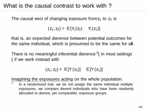
What is the causal contrast to work with ?
The causal effect of changing exposure from z1 to z2 is
δ(z1, z2) = E[Yi(z2)− Yi(z1)]
that is, an expected difference between potential outcomes forthe same individual, which is presumed to be the same for all i.
There is no meaningful inferential difference3– in most settings– if we work instead with
δ(z1, z2) = E[Y (z2)]−E[Y (z1)]
imagining the exposures acting on the whole population.3 In a randomized trial, we do not assign the same individual multiple
exposures, we compare different individuals who have been randomlyallocated to different, yet comparable, exposure groups.
180
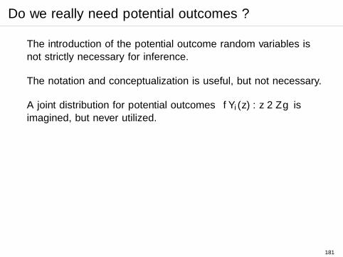
Do we really need potential outcomes ?
The introduction of the potential outcome random variables isnot strictly necessary for inference.
The notation and conceptualization is useful, but not necessary.
A joint distribution for potential outcomes {Yi(z) : z ∈ Z} isimagined, but never utilized.
181
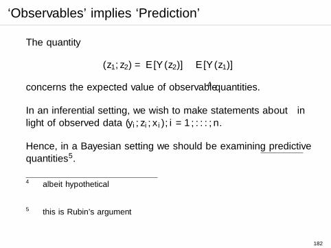
‘Observables’ implies ‘Prediction’
The quantity
δ(z1, z2) = E[Y (z2)]−E[Y (z1)]
concerns the expected value of observable4 quantities.
In an inferential setting, we wish to make statements about µ inlight of observed data (yi, zi, xi), i = 1, . . . , n.
Hence, in a Bayesian setting we should be examining predictivequantities5.
4 albeit hypothetical
5 this is Rubin’s argument
182
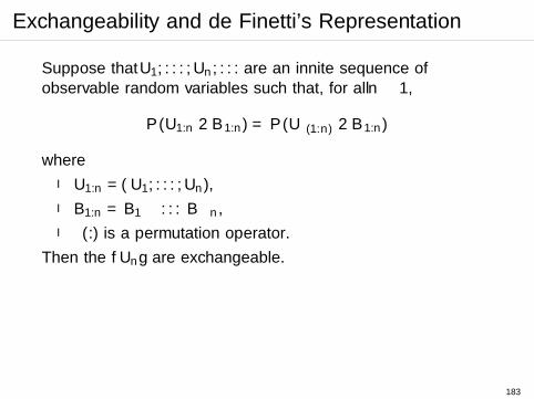
Exchangeability and de Finetti’s Representation
Suppose that U1, . . . , Un, . . . are an infinite sequence ofobservable random variables such that, for all n ≥ 1,
P (U1:n ∈ B1:n) = P (Uρ(1:n) ∈ B1:n)
where
I U1:n = (U1, . . . , Un),
I B1:n = B1 × . . .× Bn,
I ρ(.) is a permutation operator.
Then the {Un} are exchangeable.
183
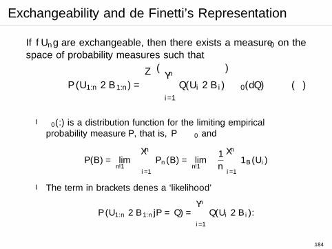
Exchangeability and de Finetti’s Representation
If {Un} are exchangeable, then there exists a measure π0 on thespace of probability measures such that
P (U1:n ∈ B1:n) =
∫ { n∏i=1
Q(Ui ∈ Bi)
}π0(dQ) (�)
I π0(.) is a distribution function for the limiting empiricalprobability measure P, that is, P ∼ π0 and
P(B) = limn−→∞
n∑i=1
Pn(B) = limn−→∞
1
n
n∑i=1
1B(Ui)
I The term in brackets defines a ‘likelihood’
P (U1:n ∈ B1:n|P = Q) =n∏
i=1
Q(Ui ∈ Bi).
184
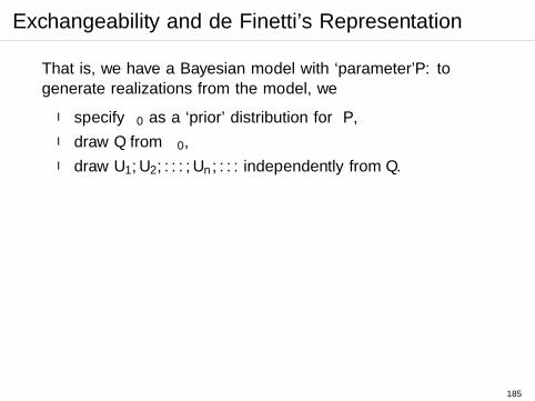
Exchangeability and de Finetti’s Representation
That is, we have a Bayesian model with ‘parameter’ P: togenerate realizations from the model, we
I specify π0 as a ‘prior’ distribution for P,
I draw Q from π0,
I draw U1, U2, . . . , Un, . . . independently from Q.
185
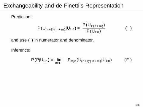
Exchangeability and de Finetti’s Representation
Prediction:
P (U(n+1):(n+m)|U1:n) =P (U1:(n+m))
P (U1:n)(�)
and use (�) in numerator and denominator.
Inference:
P (P|U1:n) = limm−→∞
Pm|n(U(n+1):(n+m)|U1:n) (F)
186
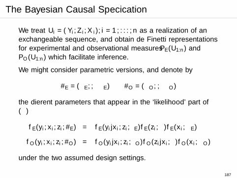
The Bayesian Causal Specification
We treat Ui = (Yi, Zi, Xi), i = 1, . . . , n as a realization of anexchangeable sequence, and obtain de Finetti representationsfor experimental and observational measures PE(U1:n) andPO(U1:n) which facilitate inference.
We might consider parametric versions, and denote by
ϑE = (θE , α, ψE) ϑO = (θO, γ, ψO)
the different parameters that appear in the ‘likelihood’ part of(�)
fE(yi, xi, zi;ϑE) = fE(yi|xi, zi; θE)fE(zi;α)fE(xi;ψE)
fO(yi, xi, zi;ϑO) = fO(yi|xi, zi; θO)fO(zi|xi; γ)fO(xi;ψO)
under the two assumed design settings.
187
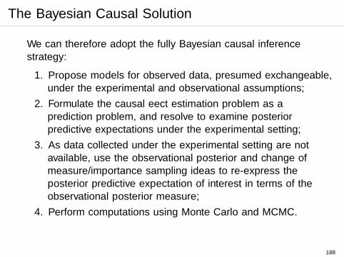
The Bayesian Causal Solution
We can therefore adopt the fully Bayesian causal inferencestrategy:
1. Propose models for observed data, presumed exchangeable,under the experimental and observational assumptions;
2. Formulate the causal effect estimation problem as aprediction problem, and resolve to examine posteriorpredictive expectations under the experimental setting;
3. As data collected under the experimental setting are notavailable, use the observational posterior and change ofmeasure/importance sampling ideas to re-express theposterior predictive expectation of interest in terms of theobservational posterior measure;
4. Perform computations using Monte Carlo and MCMC.
188
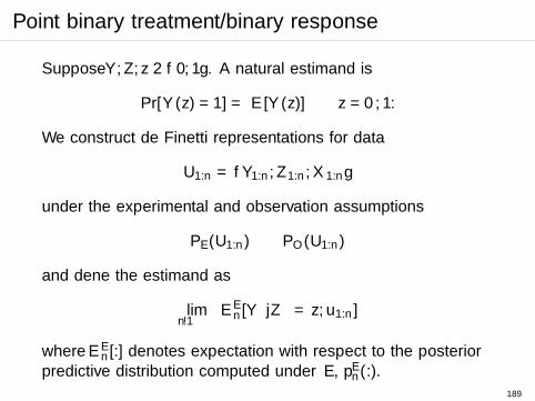
Point binary treatment/binary response
Suppose Y,Z, z ∈ {0, 1}. A natural estimand is
Pr[Y (z) = 1] = E[Y (z)] z = 0, 1.
We construct de Finetti representations for data
U1:n = {Y1:n, Z1:n, X1:n}
under the experimental and observation assumptions
PE(U1:n) PO(U1:n)
and define the estimand as
limn−→∞
EEn[Y ∗|Z∗ = z, u1:n]
where EEn[.] denotes expectation with respect to the posteriorpredictive distribution computed under E , pEn(.).
189
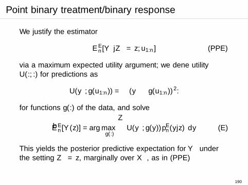
Point binary treatment/binary response
We justify the estimator
EEn[Y ∗|Z∗ = z, u1:n] (PPE)
via a maximum expected utility argument; we define utilityU(., .) for predictions as
U(y∗, g(u1:n)) = −(y∗ − g(u1:n))2.
for functions g(.) of the data, and solve
EEn[Y (z)] = arg max
g(.)
∫U(y∗, g(y))pEn(y|z) dy (E)
This yields the posterior predictive expectation for Y ∗ underthe setting Z∗ = z, marginally over X∗, as in (PPE)
190
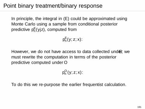
Point binary treatment/binary response
In principle, the integral in (E) could be approximated usingMonte Carlo using a sample from conditional posteriorpredictive pEn(y|z), computed from
pEn(y, z, x).
However, we do not have access to data collected under E ; wemust rewrite the computation in terms of the posteriorpredictive computed under O
pOn (y, z, x).
To do this we re-purpose the earlier frequentist calculation.
191
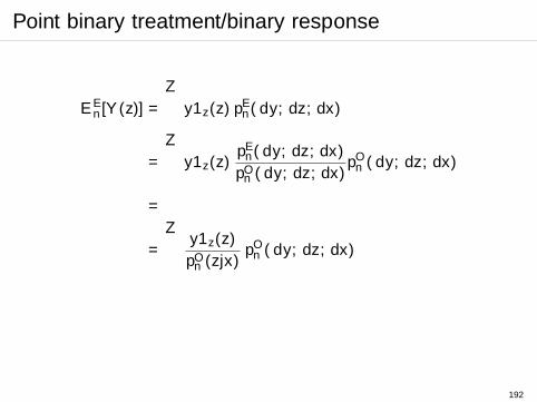
Point binary treatment/binary response
EEn[Y (z)] =
∫y1z(z) p
En( dy, dz, dx)
=
∫y1z(z)
pEn( dy, dz, dx)
pOn ( dy, dz, dx)pOn ( dy, dz, dx)
= · · ·
=
∫y1z(z)
pOn (z|x)pOn ( dy, dz, dx)
192
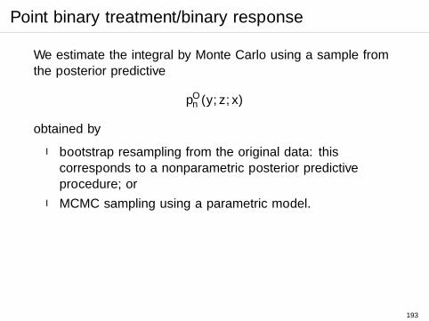
Point binary treatment/binary response
We estimate the integral by Monte Carlo using a sample fromthe posterior predictive
pOn (y, z, x)
obtained by
I bootstrap resampling from the original data: thiscorresponds to a nonparametric posterior predictiveprocedure; or
I MCMC sampling using a parametric model.
193
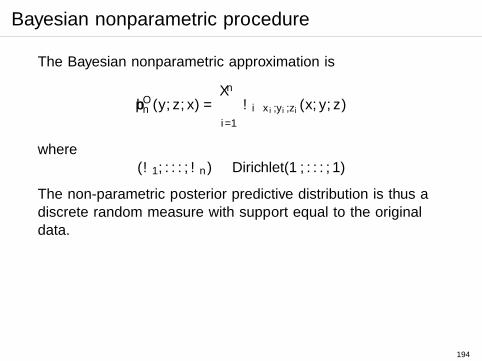
Bayesian nonparametric procedure
The Bayesian nonparametric approximation is
pOn (y, z, x) =
n∑i=1
ωiδxi,yi,zi(x, y, z)
where(ω1, . . . , ωn) ∼ Dirichlet(1, . . . , 1)
The non-parametric posterior predictive distribution is thus adiscrete random measure with support equal to the originaldata.
194
Bayesian nonparametric procedure
To produce a sample from this distribution, we first sample theω from the Dirichlet, and then (x∗, y∗, z∗) from the Multinomialdistribution on the original data with probabilities ω.
We then repeat this N times to get a sample of size N from theposterior predictive.
195
Bayesian nonparametric procedure
Now the expression
pOn (y, z, x) =
n∑i=1
ωiδxi,yi,zi(x, y, z)
implies an expression for the conditional pOn (z|x) of
pOn (z|x) =
n∑i=1
ωiδxi,zi(x, z)
n∑i=1
ωiδxi(x)
where this expression may be evaluated for x = xi i = 1, . . . , n,for each z.
196
Bayesian nonparametric procedure
This can be rewritten
pOn (z|x) =
n∑i=1
ωiδxi(x)n∑j=1
ωjδxj (x)
δzi(z)
This is also a random measure, and it will vary with each drawof ω.
197
Parametric version
In the parametric version
pOn (y, z, x) =
∫fO(y, x, z|β, α)πOn (β, α) dβ dα
=
{∫fO(y|x, z, β)πOn (β) dβ
}{∫fO(z|x, α)πOn (α) dα
}pOn (x)
= pOn (y|z, x)pOn (z|x)pOn (x)
In the calculation, the posterior predictive density
pOn (z|x) =
∫fOZ|X(z|x, α)πOn (α) dα
is typically computed using MCMC.
198
Real Data Example : ART interruption in HIV/HCV co-infected individuals
The following table shows the results for alternative estimatorsfor the interruption effect in a marginal model
fE(Yij = 1 | z, θ) = expit{θ0 + θ1z},
and the corresponding standard errors.
I The weights in the multiple imputation type estimator, aswell as in the two Bayesian estimators were calculated fromsamples of size 2500 from the posterior distributions
I Flat improper priors were used for all parameters.
I Multinomial, Dirichlet and bootstrap estimates werecalculated from 2500 replications.
199
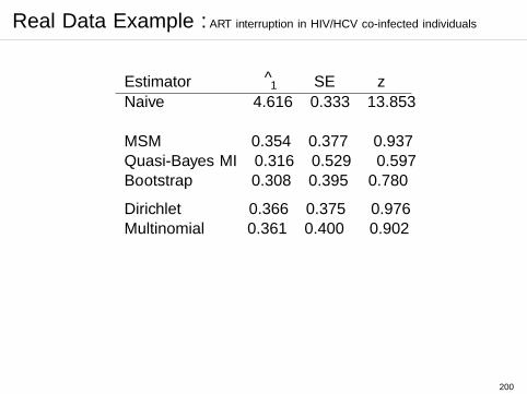
Real Data Example : ART interruption in HIV/HCV co-infected individuals
Estimator θ1 SE z
Naive 4.616 0.333 13.853
MSM 0.354 0.377 0.937Quasi-Bayes MI 0.316 0.529 0.597Bootstrap 0.308 0.395 0.780
Dirichlet 0.366 0.375 0.976Multinomial 0.361 0.400 0.902
200
Real Data Example : ART interruption in HIV/HCV co-infected individuals
The five alternative estimates are similar, with the exception ofthe MI-type estimator, which appears to inflate the standarderror. This indicates that sampling from a quasi-posterior inthe two-step approach introduces excess variability to theestimation.
In contrast, the Multinomial and Dirichlet sampling standarderrors are close to the bootstrap standard error, withoutinvolving re-estimation of the treatment assignment andcensoring models in each replication.
201