propensity score matching and analysis · what is a propensity score? a propensity score is the...
TRANSCRIPT

Propensity Score
Matching and AnalysisTEXAS EVALUATION NETWORK INSTITUTE
AUSTIN, TX
NOVEMBER 9, 2018

Schedule and outline
1:00 Introduction and overview
1:15 Quasi-experimental vs. experimental designs
1:30 Theory of propensity score methods
1:45 Computing propensity scores
2:30 Methods of matching
3:00 15 minute break
3:15 Assessing covariate balance
3:30 Estimating and matching with Stata
3:45 Q&A
4:00 Workshop ends

Introduction
Observational studies
History and development
Randomized experiments
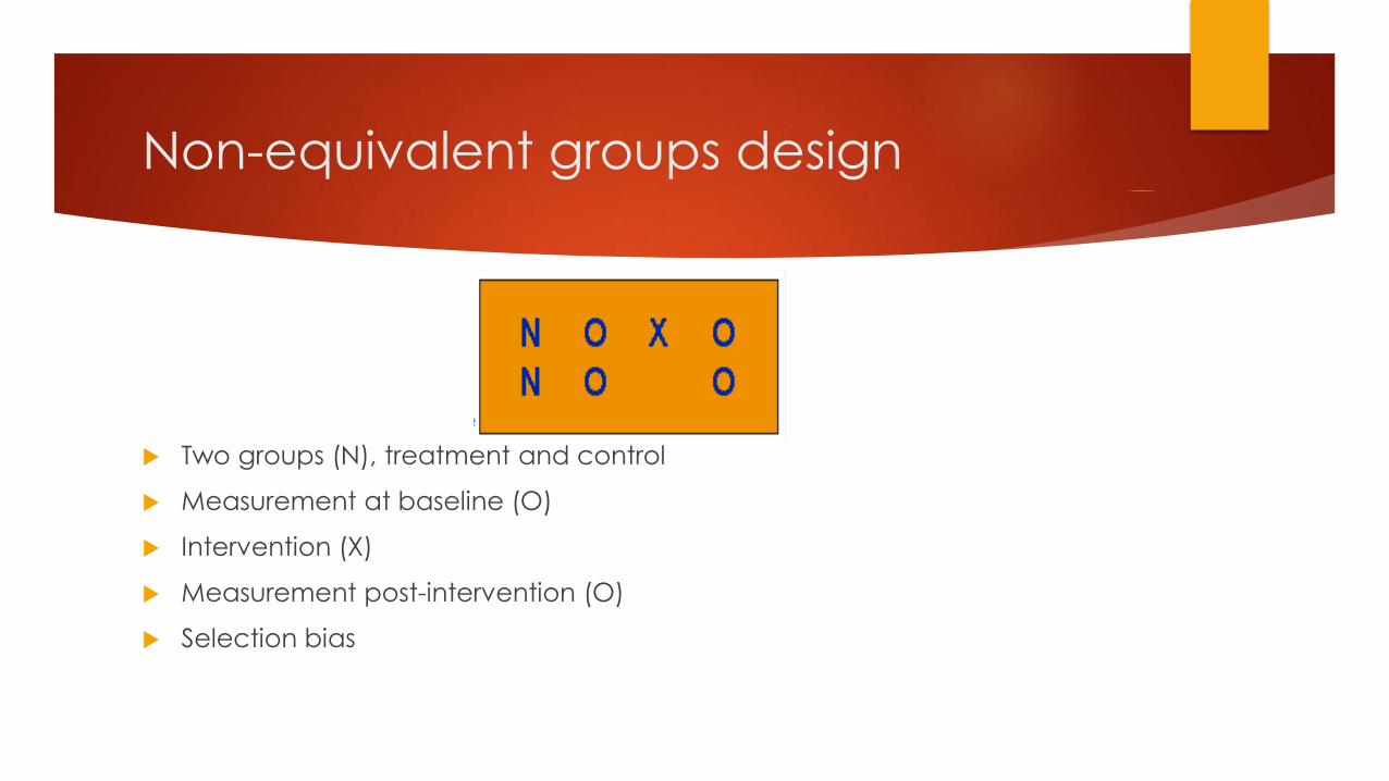
Non-equivalent groups design
Two groups (N), treatment and control
Measurement at baseline (O)
Intervention (X)
Measurement post-intervention (O)
Selection bias
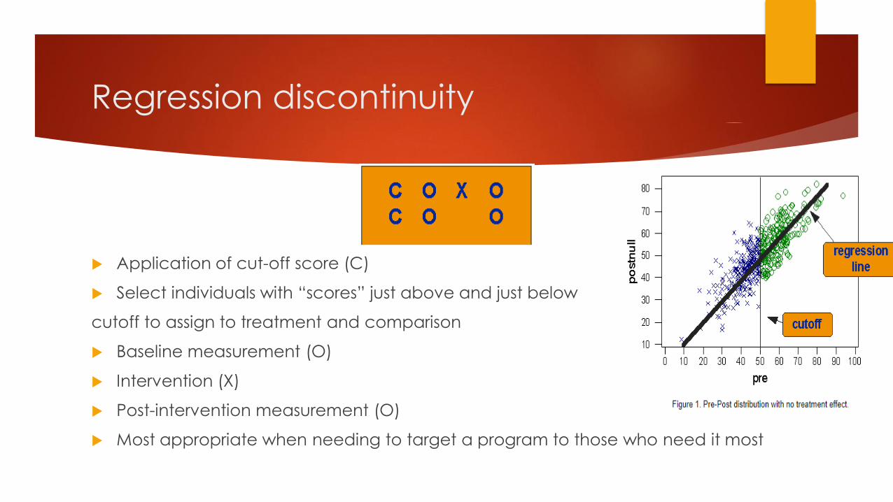
Regression discontinuity
Application of cut-off score (C)
Select individuals with “scores” just above and just below
cutoff to assign to treatment and comparison
Baseline measurement (O)
Intervention (X)
Post-intervention measurement (O)
Most appropriate when needing to target a program to those who need it most

Proxy pre-test design
Pre-test data collected after program is delivered
“recollection” proxy– ask participants where their pre-test level would
have been, or
Use administrative records from prior to program to create a proxy for a
pre-test
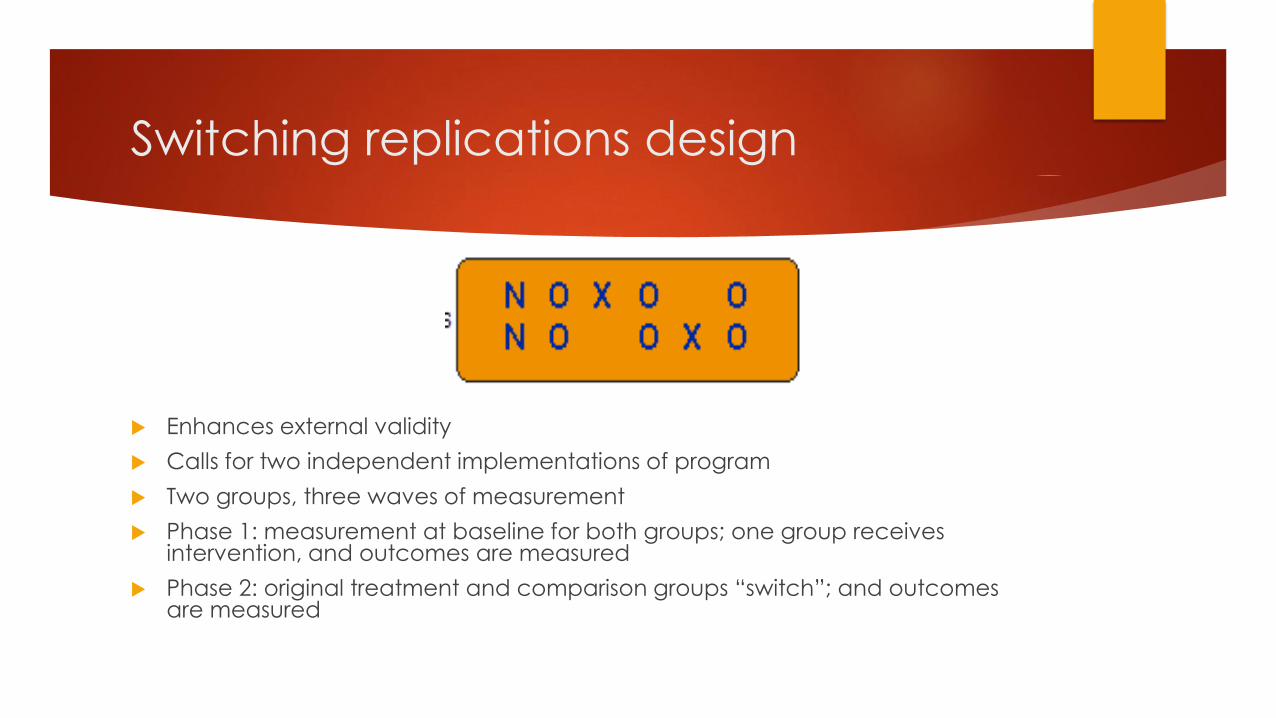
Switching replications design
Enhances external validity
Calls for two independent implementations of program
Two groups, three waves of measurement
Phase 1: measurement at baseline for both groups; one group receives intervention, and outcomes are measured
Phase 2: original treatment and comparison groups “switch”; and outcomes are measured
Others
Non-equivalent dependent variables design
Regression point displacement design
Counterfactual framework and
assumptions
Causality, internal validity, threats
Counterfactuals and the Counterfactual Framework
Measuring treatment effects
Permits us to estimate the causal effect of a treatment on an outcome using
observational (quasi-experimental) data
Scientific rationale/hypothesis is required
Counterfactual framework and
assumptions
Types of treatment effects
Average Treatment Effect (ATE)
Average Treatment Effect on the Treated (ATT)
Others (treatment effect on untreated, marginal treatment effect, local
average treatment effect, etc.)
Propensity Score Matching and
Related Models
Overview
The problem of dimensionality and the properties of propensity scores
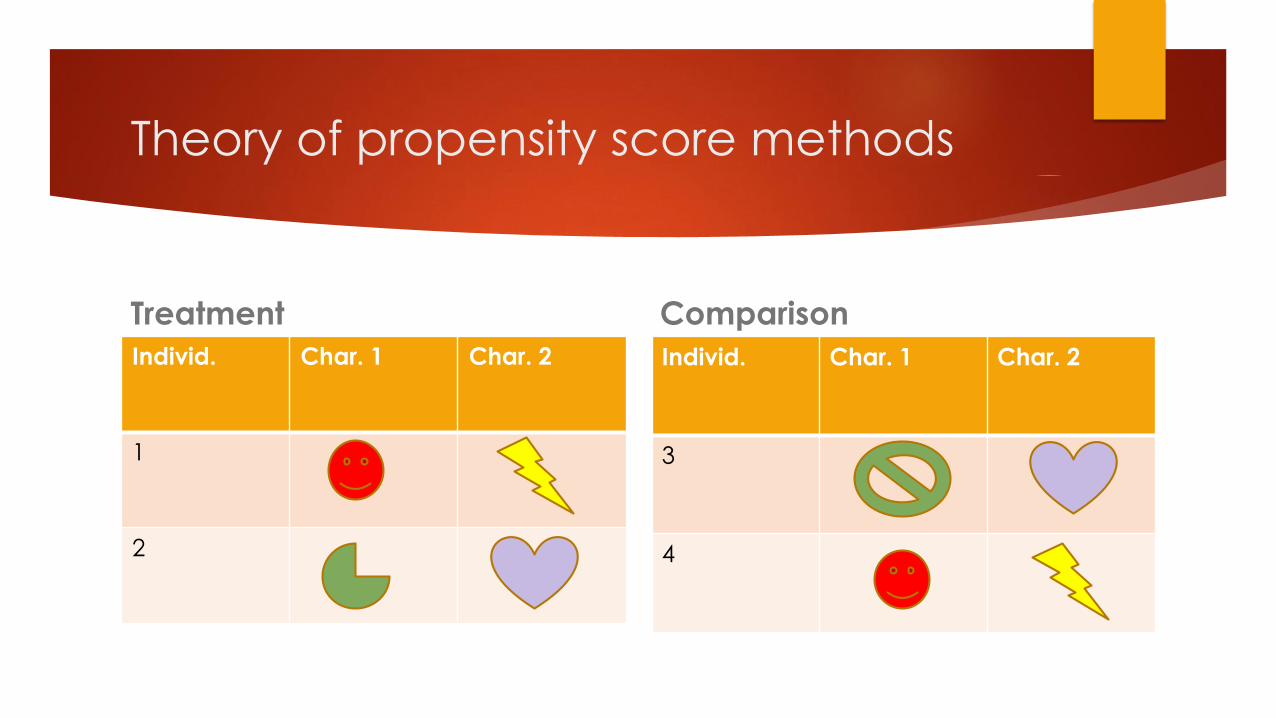
Theory of propensity score methods
Treatment
Individ. Char. 1 Char. 2
1
2
Comparison
Individ. Char. 1 Char. 2
3
4
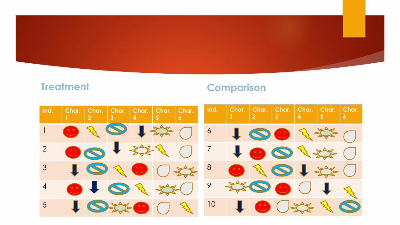
Treatment
Ind. Char. 1
Char. 2
Char. 3
Char. 4
Char. 5
Char. 6
1
2
3
4
5
Comparison
Ind. Char. 1
Char. 2
Char. 3
Char. 4
Char. 5
Char. 6
6
7
8
9
10
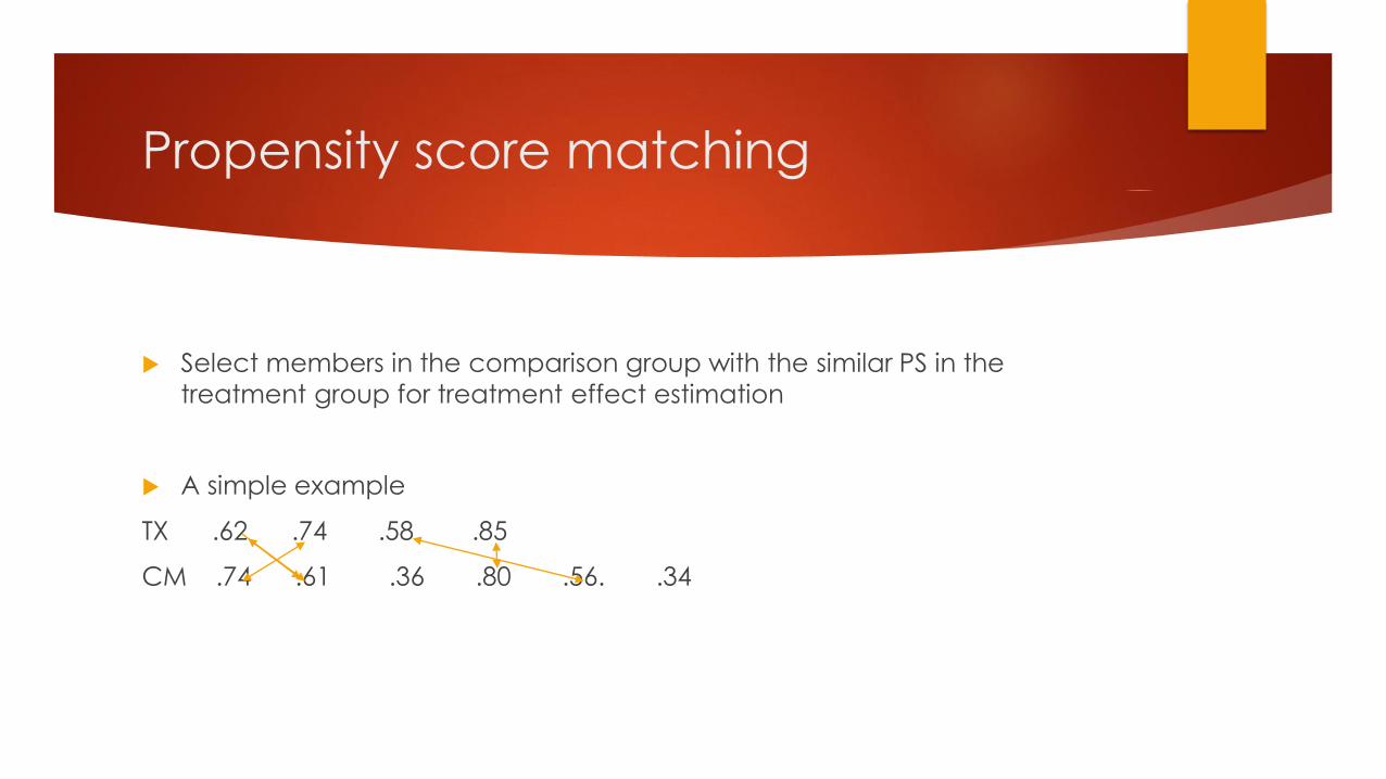
Propensity score matching
Select members in the comparison group with the similar PS in the
treatment group for treatment effect estimation
A simple example
TX .62 .74 .58 .85
CM .74 .61 .36 .80 .56. .34
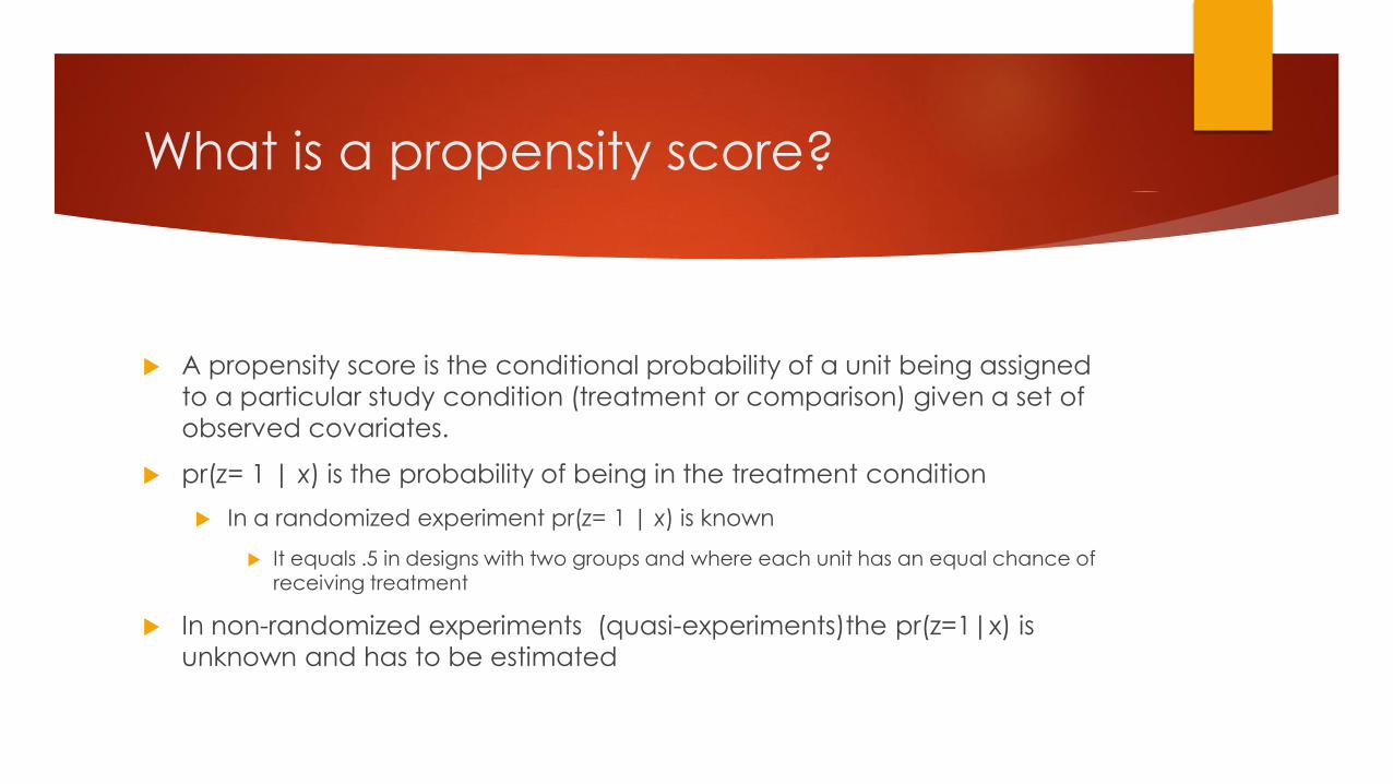
What is a propensity score?
A propensity score is the conditional probability of a unit being assigned
to a particular study condition (treatment or comparison) given a set of
observed covariates.
pr(z= 1 | x) is the probability of being in the treatment condition
In a randomized experiment pr(z= 1 | x) is known
It equals .5 in designs with two groups and where each unit has an equal chance of receiving treatment
In non-randomized experiments (quasi-experiments)the pr(z=1|x) is
unknown and has to be estimated

Propensity Score Matching and
Related Models
Matching
Greedy matching
Optimal matching
Fine balance
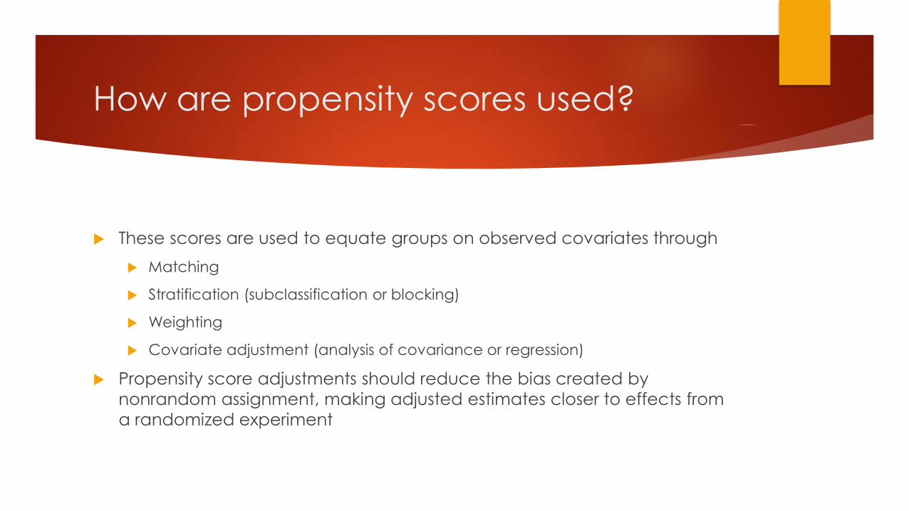
How are propensity scores used?
These scores are used to equate groups on observed covariates through
Matching
Stratification (subclassification or blocking)
Weighting
Covariate adjustment (analysis of covariance or regression)
Propensity score adjustments should reduce the bias created by
nonrandom assignment, making adjusted estimates closer to effects from
a randomized experiment
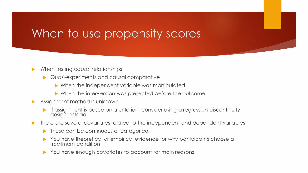
When to use propensity scores
When testing causal relationships
Quasi-experiments and causal comparative
When the independent variable was manipulated
When the intervention was presented before the outcome
Assignment method is unknown
If assignment is based on a criterion, consider using a regression discontinuity design instead
There are several covariates related to the independent and dependent variables
These can be continuous or categorical
You have theoretical or empirical evidence for why participants choose a treatment condition
You have enough covariates to account for main reasons
When not to use propensity scores
Propensity Score Matching and
Related Models
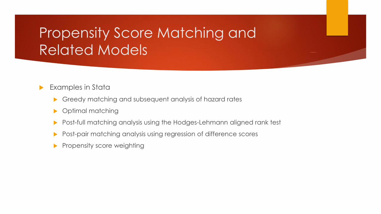
Examples in Stata
Greedy matching and subsequent analysis of hazard rates
Optimal matching
Post-full matching analysis using the Hodges-Lehmann aligned rank test
Post-pair matching analysis using regression of difference scores
Propensity score weighting
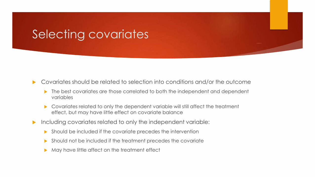
Selecting covariates
Covariates should be related to selection into conditions and/or the outcome
The best covariates are those correlated to both the independent and dependent
variables
Covariates related to only the dependent variable will still affect the treatment
effect, but may have little effect on covariate balance
Including covariates related to only the independent variable:
Should be included if the covariate precedes the intervention
Should not be included if the treatment precedes the covariate
May have little affect on the treatment effect
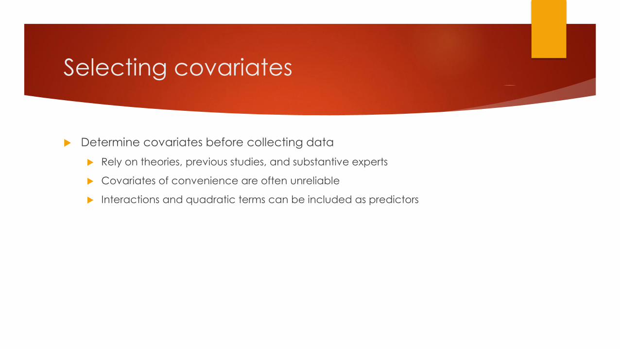
Selecting covariates
Determine covariates before collecting data
Rely on theories, previous studies, and substantive experts
Covariates of convenience are often unreliable
Interactions and quadratic terms can be included as predictors
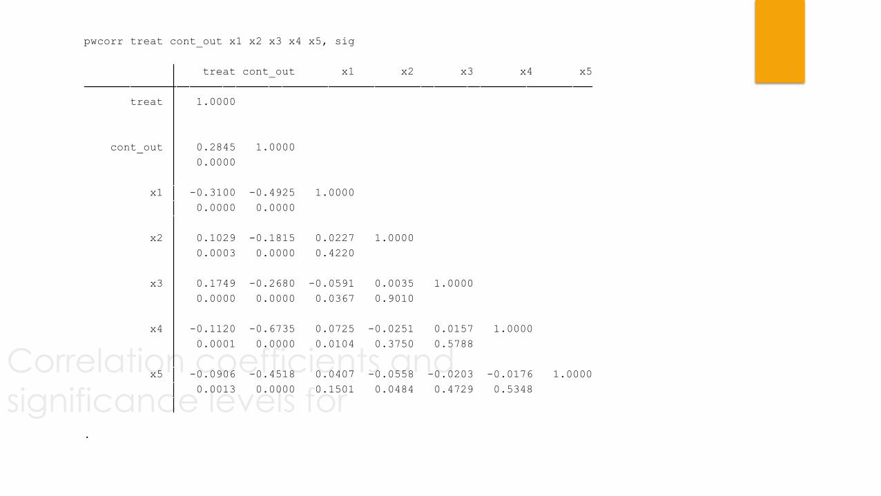
Correlation coefficients and
significance levels for .
0.0013 0.0000 0.1501 0.0484 0.4729 0.5348
x5 -0.0906 -0.4518 0.0407 -0.0558 -0.0203 -0.0176 1.0000
0.0001 0.0000 0.0104 0.3750 0.5788
x4 -0.1120 -0.6735 0.0725 -0.0251 0.0157 1.0000
0.0000 0.0000 0.0367 0.9010
x3 0.1749 -0.2680 -0.0591 0.0035 1.0000
0.0003 0.0000 0.4220
x2 0.1029 -0.1815 0.0227 1.0000
0.0000 0.0000
x1 -0.3100 -0.4925 1.0000
0.0000
cont_out 0.2845 1.0000
treat 1.0000
treat cont_out x1 x2 x3 x4 x5
pwcorr treat cont_out x1 x2 x3 x4 x5, sig
Balancing propensity scores
Identify “area of common support”
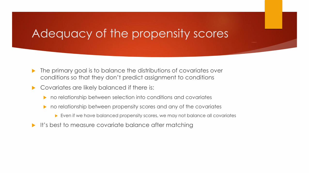
Adequacy of the propensity scores
The primary goal is to balance the distributions of covariates over
conditions so that they don’t predict assignment to conditions
Covariates are likely balanced if there is:
no relationship between selection into conditions and covariates
no relationship between propensity scores and any of the covariates
Even if we have balanced propensity scores, we may not balance all covariates
It’s best to measure covariate balance after matching

Demonstration in Stata

Step 1: Creating the propensity score
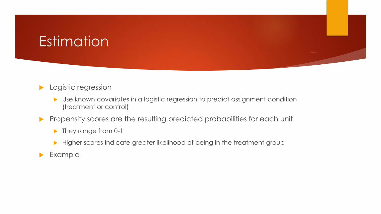
Estimation
Logistic regression
Use known covariates in a logistic regression to predict assignment condition
(treatment or control)
Propensity scores are the resulting predicted probabilities for each unit
They range from 0-1
Higher scores indicate greater likelihood of being in the treatment group
Example
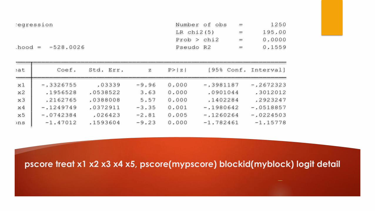
pscore treat x1 x2 x3 x4 x5, pscore(mypscore) blockid(myblock) logit detail
_cons -1.47012 .1593604 -9.23 0.000 -1.782461 -1.15778
x5 -.0742384 .026423 -2.81 0.005 -.1260264 -.0224503
x4 -.1249749 .0372911 -3.35 0.001 -.1980642 -.0518857
x3 .2162765 .0388008 5.57 0.000 .1402284 .2923247
x2 .1956528 .0538522 3.63 0.000 .0901044 .3012012
x1 -.3326755 .03339 -9.96 0.000 -.3981187 -.2672323
treat Coef. Std. Err. z P>|z| [95% Conf. Interval]
Log likelihood = -528.0026 Pseudo R2 = 0.1559
Prob > chi2 = 0.0000
LR chi2(5) = 195.00
Logistic regression Number of obs = 1250
Step Two: Balance of Propensity Score
across Treatment and Comparison Groups
Ensure that there is overlap in the range of propensity scores across
treatment and comparison groups (the “area of common support”)
Subjectively assessed (eyeballed) by examining graph of propensity scores for
treatment and comparison groups
75% overlap is considered good
Distribution of treatment and comparison propensity scores should be
balanced
Ensure that mean propensity score is equivalent in both treatment and
comparison
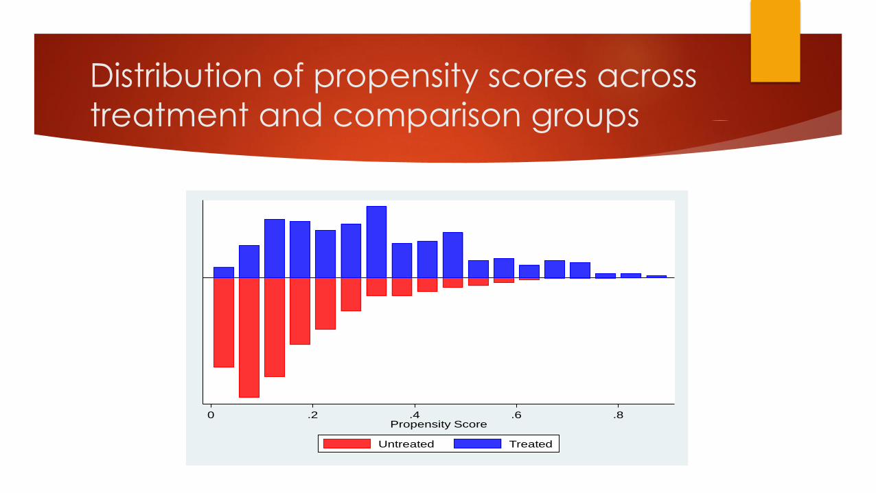
Distribution of propensity scores across
treatment and comparison groups
0 .2 .4 .6 .8Propensity Score
Untreated Treated
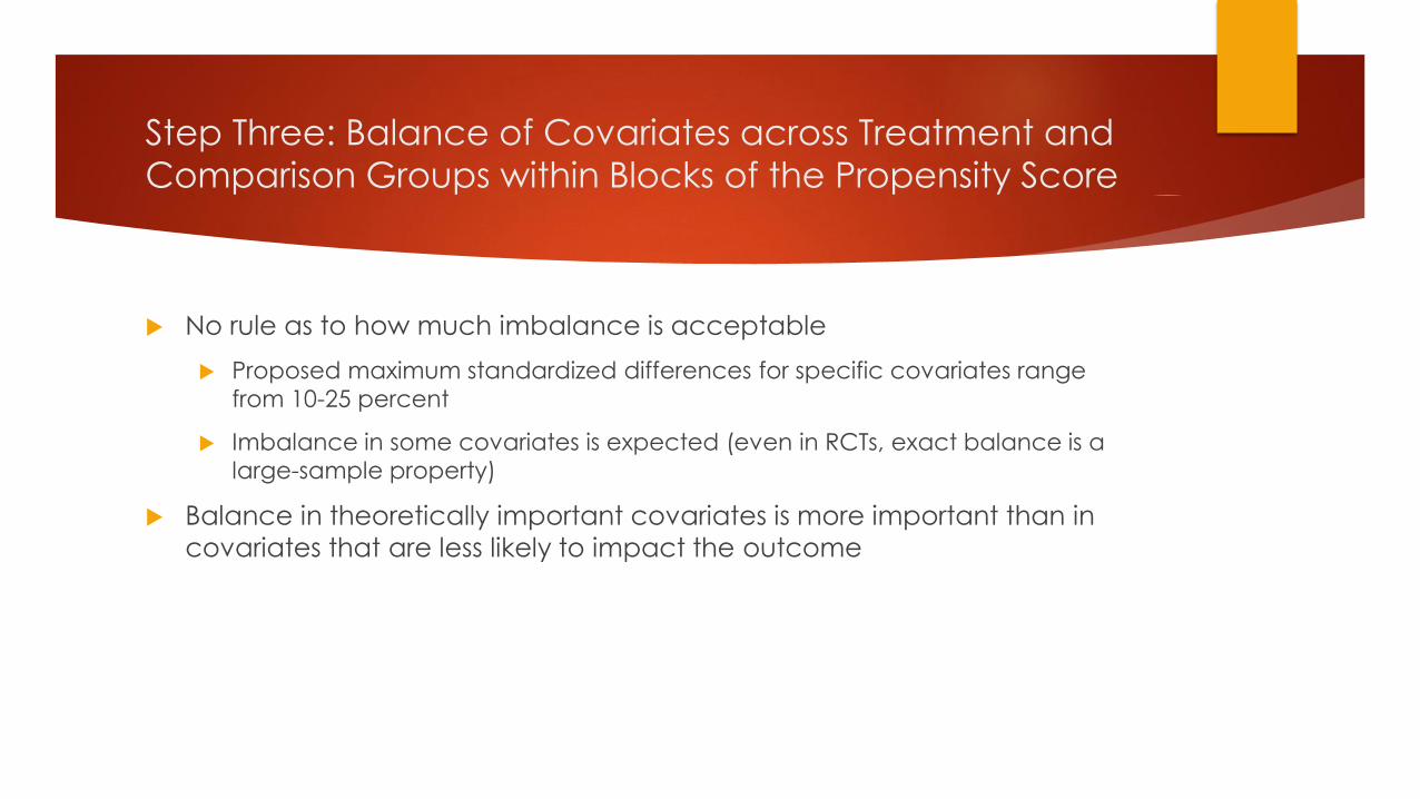
Step Three: Balance of Covariates across Treatment and
Comparison Groups within Blocks of the Propensity Score
No rule as to how much imbalance is acceptable
Proposed maximum standardized differences for specific covariates range
from 10-25 percent
Imbalance in some covariates is expected (even in RCTs, exact balance is a
large-sample property)
Balance in theoretically important covariates is more important than in
covariates that are less likely to impact the outcome
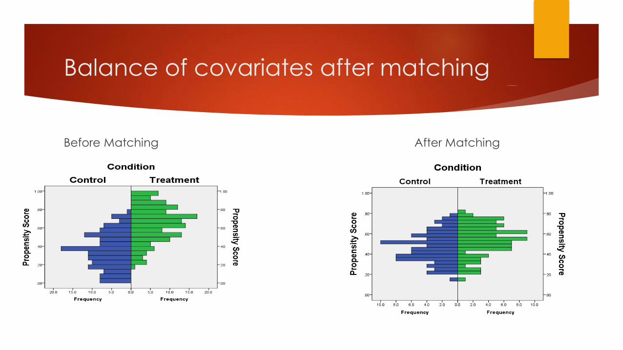
Balance of covariates after matching
Before Matching After Matching

Step Four: Choice of weighting
strategies

Types of “Greedy Matching”
Nearest Neighbor
Caliper
Mahalanobis with Propensity Score
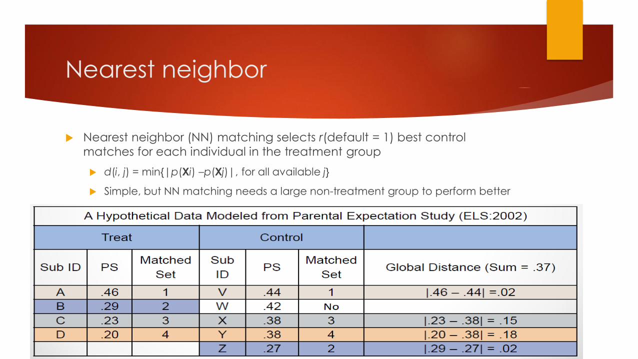
Nearest neighbor
Nearest neighbor (NN) matching selects r(default = 1) best control
matches for each individual in the treatment group
d(i, j) = min{|p(Xi) –p(Xj)|, for all available j}
Simple, but NN matching needs a large non-treatment group to perform better
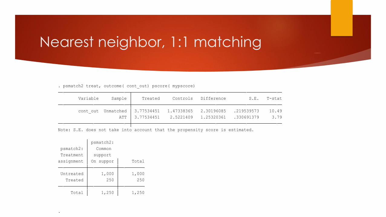
.
Total 1,250 1,250
Treated 250 250
Untreated 1,000 1,000
assignment On suppor Total
Treatment support
psmatch2: Common
psmatch2:
Note: S.E. does not take into account that the propensity score is estimated.
ATT 3.77534451 2.5221409 1.25320361 .330691379 3.79
cont_out Unmatched 3.77534451 1.47338365 2.30196085 .219539573 10.49
Variable Sample Treated Controls Difference S.E. T-stat
. psmatch2 treat, outcome( cont_out) pscore( mypscore)
Nearest neighbor, 1:1 matching
Caliper
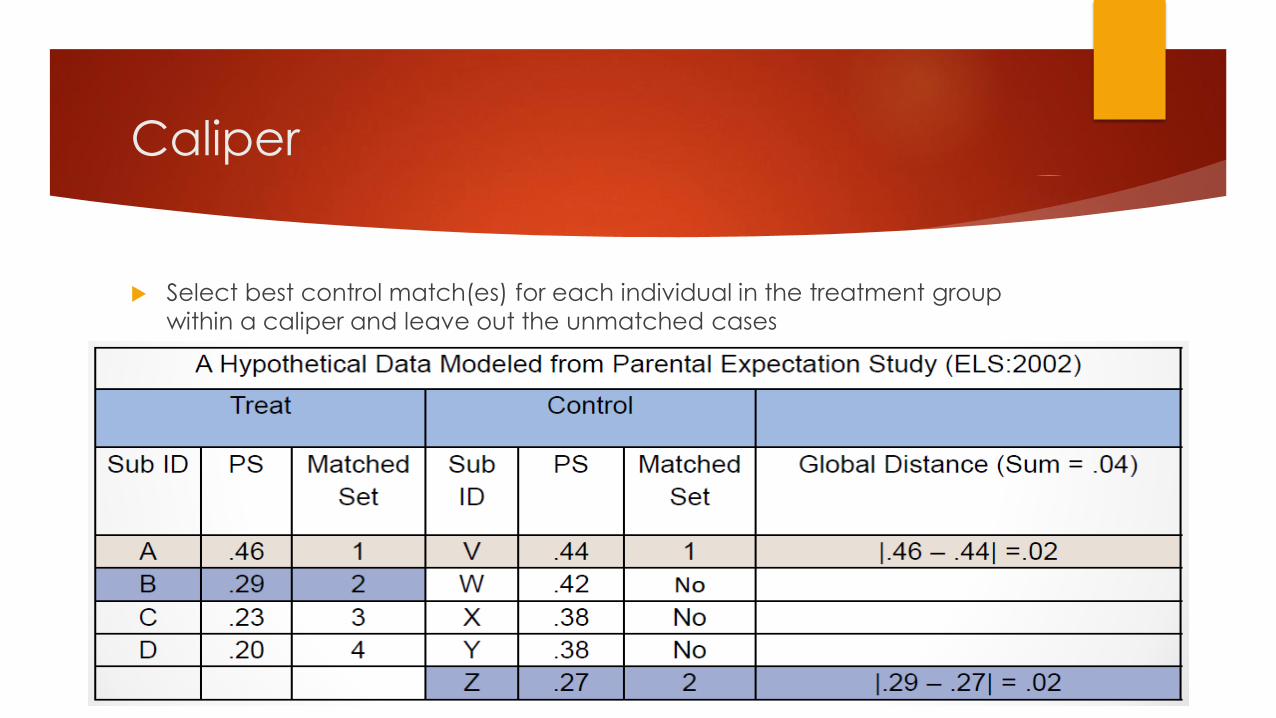
Select best control match(es) for each individual in the treatment group
within a caliper and leave out the unmatched cases
Caliper, cont.
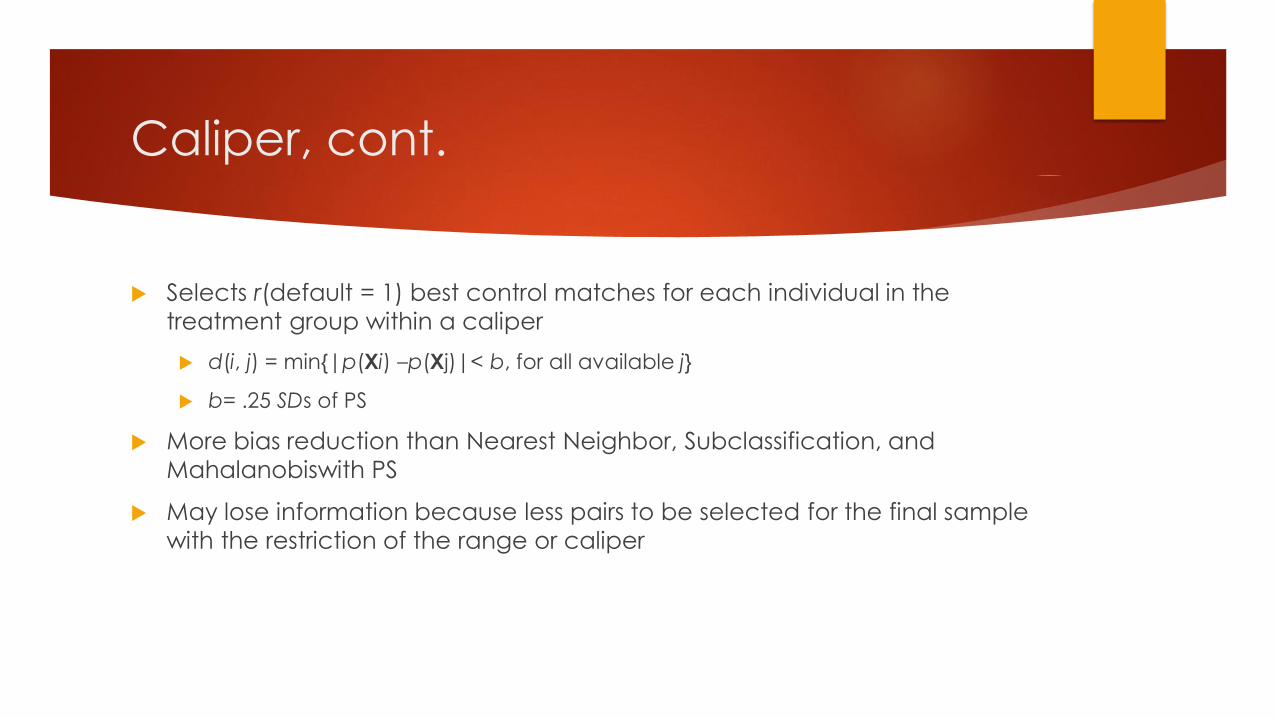
Selects r(default = 1) best control matches for each individual in the
treatment group within a caliper
d(i, j) = min{|p(Xi) –p(Xj)|< b, for all available j}
b= .25 SDs of PS
More bias reduction than Nearest Neighbor, Subclassification, and
Mahalanobiswith PS
May lose information because less pairs to be selected for the final sample
with the restriction of the range or caliper
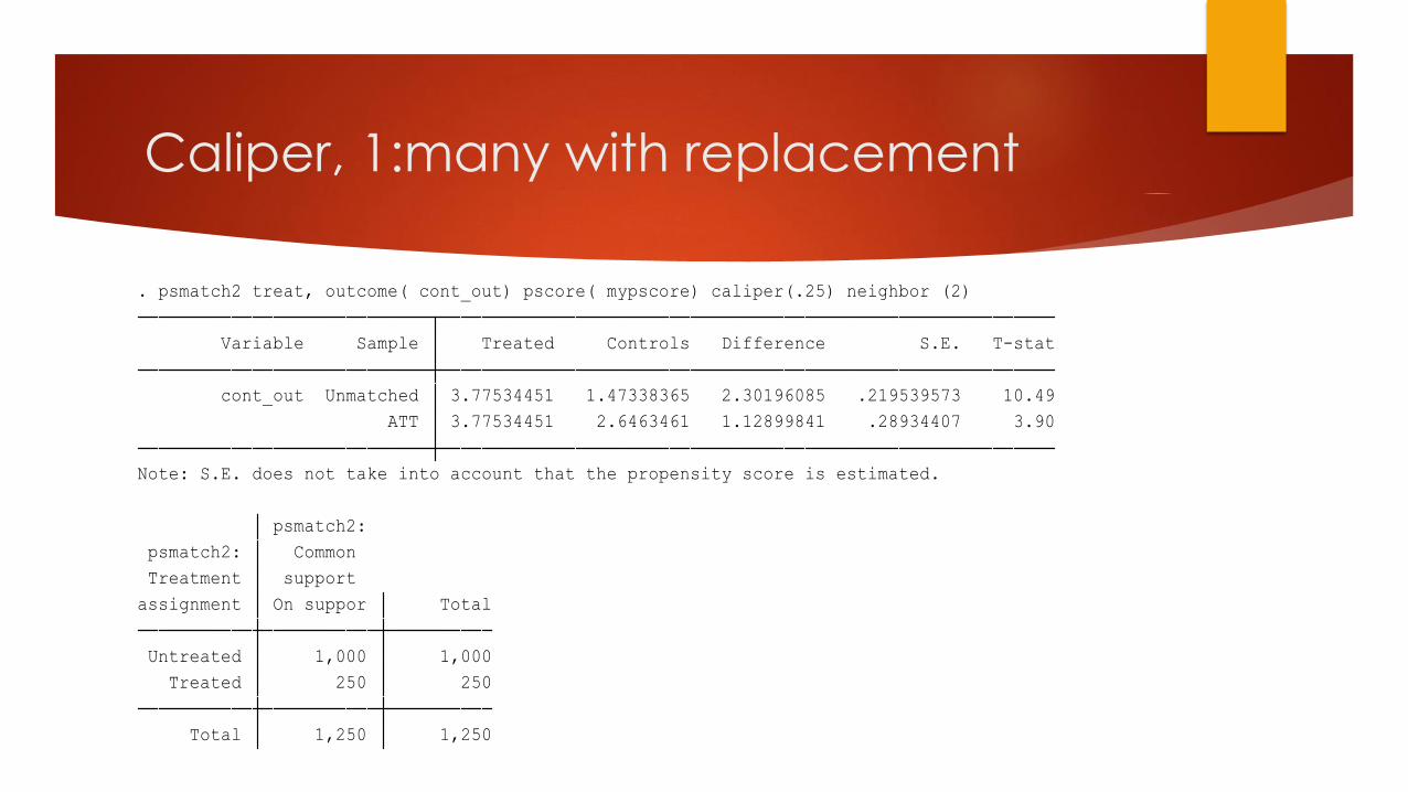
Caliper, 1:many with replacement
Total 1,250 1,250
Treated 250 250
Untreated 1,000 1,000
assignment On suppor Total
Treatment support
psmatch2: Common
psmatch2:
Note: S.E. does not take into account that the propensity score is estimated.
ATT 3.77534451 2.6463461 1.12899841 .28934407 3.90
cont_out Unmatched 3.77534451 1.47338365 2.30196085 .219539573 10.49
Variable Sample Treated Controls Difference S.E. T-stat
. psmatch2 treat, outcome( cont_out) pscore( mypscore) caliper(.25) neighbor (2)
Complex Matching Types
Kernel
Optimal
Subclassification
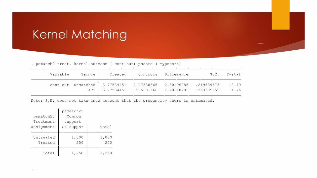
Kernel Matching
.
Total 1,250 1,250
Treated 250 250
Untreated 1,000 1,000
assignment On suppor Total
Treatment support
psmatch2: Common
psmatch2:
Note: S.E. does not take into account that the propensity score is estimated.
ATT 3.77534451 2.5691566 1.20618791 .253585952 4.76
cont_out Unmatched 3.77534451 1.47338365 2.30196085 .219539573 10.49
Variable Sample Treated Controls Difference S.E. T-stat
. psmatch2 treat, kernel outcome ( cont_out) pscore ( mypscore)
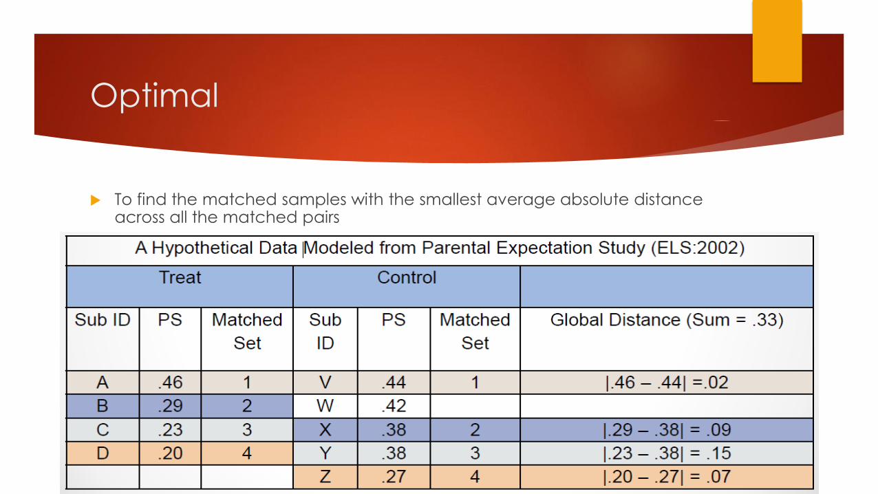
Optimal
To find the matched samples with the smallest average absolute distance across all the matched pairs
Optimal matching, cont.
Minimized global distance
The same sets of controls for overall matched samples as from greedy
matching with larger control group samples
Optimal matching can be helpful when there are not many appropriate
control matches for the treated units
Treatment sample size remains constant
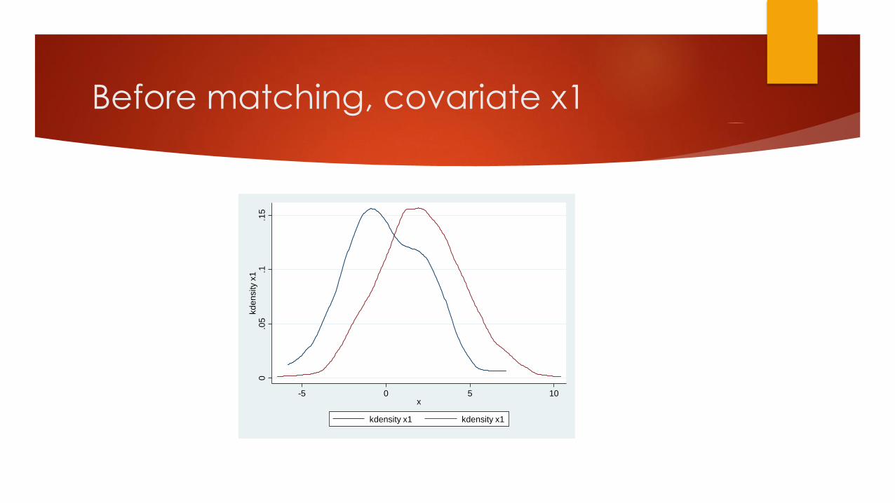
Before matching, covariate x1
0.0
5.1
.15
kd
en
sity x
1
-5 0 5 10x
kdensity x1 kdensity x1
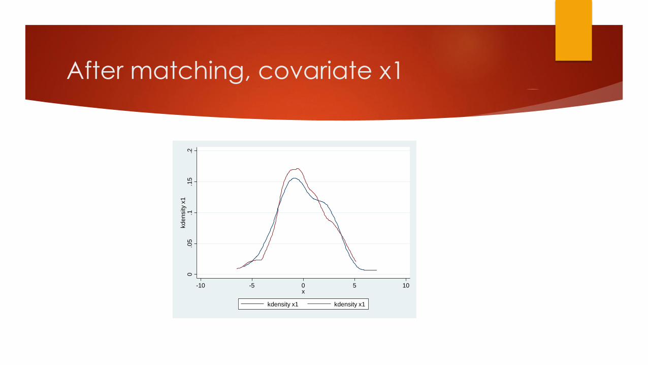
After matching, covariate x1
0.0
5.1
.15
.2kd
en
sity x
1
-10 -5 0 5 10x
kdensity x1 kdensity x1
Step Five: Balance of Covariates after Matching
or Weighting the Sample by a Propensity Score
.
* if B>25%, R outside [0.5; 2]
Matched 0.003 2.19 0.823 5.7 6.0 13.2 0.82 20
Unmatched 0.156 195.15 0.000 40.6 28.5 104.2* 0.93 0
Sample Ps R2 LR chi2 p>chi2 MeanBias MedBias B R %Var
* if variance ratio outside [0.78; 1.28] for U and [0.78; 1.28] for M
M -3.0106 -2.7974 -7.2 67.9 -0.86 0.391 1.39*
x5 U -3.0106 -2.3455 -22.5 -3.21 0.001 1.06
M -1.6722 -1.4857 -9.2 67.8 -1.02 0.310 0.89
x4 U -1.6722 -1.0928 -28.5 -3.98 0.000 0.93
M 1.9071 2.0272 -6.0 86.3 -0.66 0.510 1.04
x3 U 1.9071 1.0323 43.6 6.27 0.000 1.12
M -1.153 -1.2031 3.5 86.7 0.37 0.710 0.83
x2 U -1.153 -1.5301 26.0 3.65 0.000 0.96
M .01912 -.04552 2.6 96.8 0.30 0.762 1.11
x1 U .01912 2.0581 -82.2 -11.52 0.000 0.94
Variable Matched Treated Control %bias |bias| t p>|t| V(C)
Unmatched Mean %reduct t-test V(T)/
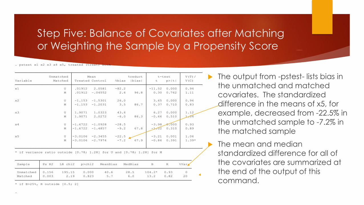
. pstest x1 x2 x3 x4 x5, treated (treat) both
The output from -pstest- lists bias in
the unmatched and matched
covariates. The standardized
difference in the means of x5, for
example, decreased from -22.5% in the unmatched sample to -7.2% in
the matched sample
The mean and median
standardized difference for all of
the covariates are summarized at the end of the output of this
command.
Step x: Estimation and interpretation of
treatment effects
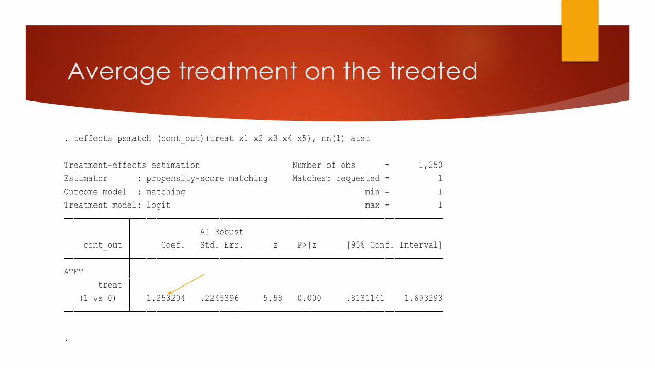
Average treatment on the treated
.
(1 vs 0) 1.253204 .2245396 5.58 0.000 .8131141 1.693293
treat
ATET
cont_out Coef. Std. Err. z P>|z| [95% Conf. Interval]
AI Robust
Treatment model: logit max = 1
Outcome model : matching min = 1
Estimator : propensity-score matching Matches: requested = 1
Treatment-effects estimation Number of obs = 1,250
. teffects psmatch (cont_out)(treat x1 x2 x3 x4 x5), nn(1) atet
Concluding remarks
Common pitfalls in observational studies: a checklist for critical review
Approximating experiments with propensity score approaches
Criticism of PSM
Criticism of sensitivity analysis
Group randomized trials
Resources
Garrido, Melissa M. et al (2014). Methods for Constructing and Assessing Propensity Scores, Health Services Research, Health Research and Educational Trust.
Guo, Shenyang and Mark W. Fraser (2010). Propensity Score Analysis: Statistical Methods and Applications. Thousand Oaks, CA: Sage Publications
Pan, W., & Bai, H. (Eds.). (2015). Propensity score analysis: Fundamentals, developments, and extensions. New York, NY: Guilford Press.
Bai, H., & M.H. Clark (in press, 2018). Propensity score methods and applications. Thousand Oaks, CA: Sage Publications
•Basic Concepts of PS Methods
•Covariate Selection and PS Estimation
•PS Adjustment Methods
•Evaluation and Analysis after Matching

Thanks
Greg Cumpton, PhD
Heath Prince, PhD