propagation of densities of streaming data within query graphs · propagation of densities of...

Propagation of Densities of Streaming Data withinQuery Graphs

Michael Daum, Frank Lauterwald, Philipp Baumgartel, Klaus Meyer-Wegener{md, frank, snphbaum, kmw}@i6.cs.fau.de

Dept. of Computer Science, University of Erlangen-Nuremberg, Germany

Abstract. Data Stream Systems (DSSs) use cost models to determine if a DSScan cope with a given workload and to optimize query graphs. However, certainrelevant input parameters of these models are often unknown or highly imprecise.Especially selectivities are stream-dependent and application-specific parameters.In this paper, we describe a method that supports selectivity estimation consid-ering input streams’ attribute value distribution. The novelty of our approach isthe propagation of the probability distributions through the query graph in or-der to give estimates for the inner nodes of the graph. For most common streamoperators, we establish formulas that describe their output distribution as a func-tion of their input distributions. For unknown operators like User-Defined Oper-ators (UDOs), we introduce a method to measure the influence of these operatorson arbitrary probability distributions. This method is able to do most of the com-putational work before the query is deployed and introduces minimal overheadat runtime. Our evaluation framework facilitates the appropriate combination ofboth methods and allows to model almost arbitrary query graphs.

1 Introduction

Over the past few years, the field of data stream research has matured, and first com-mercial products have appeared. There is still a lot of need of and potential for researchin distributing, estimating, and optimizing of queries.

Estimation of costs of data processing in data streams is crucial, especially if datastream processing is distributed over battery-powered sensor nodes. This estimationneeds to know the data rates and the distribution of values. In our project Data StreamApplication Manager (DSAM) [1], we distribute queries over a network of heteroge-neous Stream Processing Systems (SPSs) and Wireless Sensor Network (WSN) nodes.This paper presents some of the theoretical results regarding the cost estimator ofDSAM.

Like in a Database System (DBS), a query in a Data Stream System (DSS) consistsof a graph of operator instances (nodes) that are connected by inner streams. Each oper-ator in a query may manipulate both the data rate and the distribution of values in a datastream. The outgoing data rate of an operator is often influenced by the distribution ofvalues. In order to achieve good estimates for the whole query, characteristics of inter-mediate data streams between operators are also relevant. This requires the propagationof estimates through the entire graph. The manipulation of these characteristics (changeof variables’ formula) can be either measured, computed by analytic methods or it can

06.04.2010 SSDBM 2010 Camera-Ready

1/18

buettner

Schreibmaschinentext

The original publication is available at www.springer.com/computer/database+management+%26+information+retrieval/book/978-3-642-13817-1

buettner


buettner


buettner


be approximated by numerical methods. Basically, an analytic method is preferable asit is more precise and less computationally intensive. Some operators are unfortunatelynot manageable with analytic methods. For the support of complex query graphs, how-ever, it will be necessary to combine analytic and numerical propagation methods.

In simple cases, each data element of a data stream consists of one value. There aresome approaches that support density estimation of one-dimensional data stream items.Heinz and Seeger present approaches that use kernels and wavelets to estimate densitiesof one-dimensional data streams [2,3]. These approaches use measurements in order todetermine the density estimators.

To our knowledge, this is the first work addressing the propagation of densitieswithin query graphs of DSSs by using analytic or numerical methods. Further, it sup-ports multi-dimensional data stream elements. Our contribution to the problem of es-timating multi-dimensional densities operates on two levels: First, we propose bothanalytic and numerical propagation of densities for relevant streaming operators andargue which method is appropriate for each operator. Second, we propose a method forcombining these approaches as each operator has a best fitting method for propagatingdensities, but a query graph may contain both kinds of operators.

We address related work in more detail in the next section. The core of this paperstarts with basic explanations and definitions for the estimation of Probability DensityFunctions (PDFs) in Sect. 3. In the following two sections, we present the analytic prop-agation method and the numerical propagation method. We make a synthesis of thesetwo methods using Kernel Density Estimators (KDEs) that includes some experimentalresults before we conclude.

2 Related Work

There are several “historical” approaches that use probabilities for the estimation ofdatabases’ statistics. In [4], multi-dimensional histograms model attribute value distri-butions. There are several formulas for the impact of operators on distributions. Wecould not adopt these formulas directly for data streams as on the one hand they onlyconsider densities represented as histograms and on the other hand they postulate dis-crete probability distributions. As they consider databases, e.g. the projection operatoruses duplicate elimination.

The Detailed Database Statistics Model (DDSM) [5] considers one-dimensionaldiscrete distributions, but with additional matrices that represent dependencies betweensubdomains of attributes. This paper also describes statistics for estimating join sizes.The influence of operators is evaluated for selection and join.

A survey [6] gives an overview of estimation of statistical profiles in database sys-tems. This paper discusses the influence of statistical methods on cost estimation indifferent database systems. Further, it discusses different methods of density estimationand the influence of database operators on probability densities without giving concreteformulas.

As mentioned in the introduction, [2] and [3] investigated density estimators overdata streams. These papers only consider measuring densities of existing streams. The


2/18

densities of intermediate streams are still unknown, if there is no actual system execut-ing the respective query.

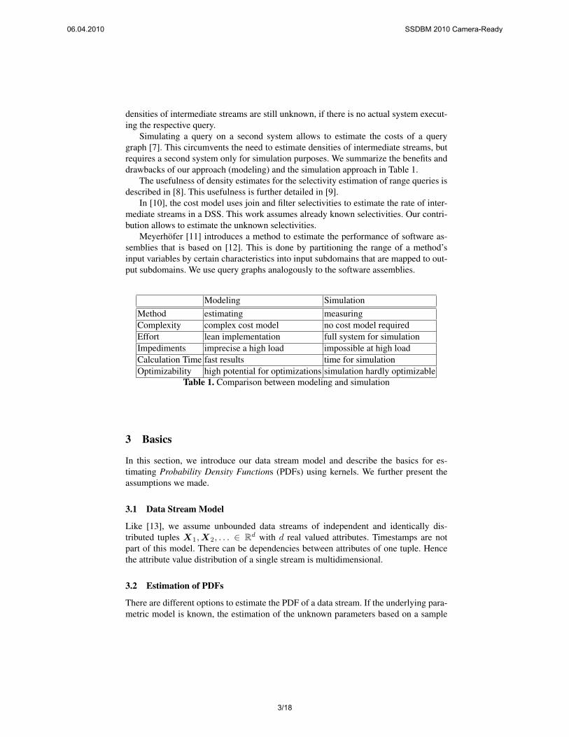
Simulating a query on a second system allows to estimate the costs of a querygraph [7]. This circumvents the need to estimate densities of intermediate streams, butrequires a second system only for simulation purposes. We summarize the benefits anddrawbacks of our approach (modeling) and the simulation approach in Table 1.

The usefulness of density estimates for the selectivity estimation of range queries isdescribed in [8]. This usefulness is further detailed in [9].

In [10], the cost model uses join and filter selectivities to estimate the rate of inter-mediate streams in a DSS. This work assumes already known selectivities. Our contri-bution allows to estimate the unknown selectivities.

Meyerhofer [11] introduces a method to estimate the performance of software as-semblies that is based on [12]. This is done by partitioning the range of a method’sinput variables by certain characteristics into input subdomains that are mapped to out-put subdomains. We use query graphs analogously to the software assemblies.

Modeling SimulationMethod estimating measuringComplexity complex cost model no cost model requiredEffort lean implementation full system for simulationImpediments imprecise a high load impossible at high loadCalculation Time fast results time for simulationOptimizability high potential for optimizations simulation hardly optimizable

Table 1. Comparison between modeling and simulation

3 Basics

In this section, we introduce our data stream model and describe the basics for es-timating Probability Density Functions (PDFs) using kernels. We further present theassumptions we made.

3.1 Data Stream Model

Like [13], we assume unbounded data streams of independent and identically dis-tributed tuples X1,X2, . . . ∈ Rd with d real valued attributes. Timestamps are notpart of this model. There can be dependencies between attributes of one tuple. Hencethe attribute value distribution of a single stream is multidimensional.

3.2 Estimation of PDFs

There are different options to estimate the PDF of a data stream. If the underlying para-metric model is known, the estimation of the unknown parameters based on a sample


3/18

is sufficient to determine the density of the stream. Nonparametric estimation is analternative approach with no need for information about the underlying model. Onewell-known example for nonparametric estimation is KDE [14, 15].

A Kernel Density Estimator (KDE) is constructed from a sampleX1,X2, . . . ,Xk with Xi = (Xi,1, . . . , Xi,d), Xi,j ∈ R as follows:

f (k)(x) =1

k

k∑i=1

d∏j=1

1

h(k)j

K

(xj −Xi,j

h(k)j

),x ∈ Rd. (1)

The kernel function K is an arbitrary one-dimensional symmetric PDF with mean0. This means that every tuple in the sample is represented by a “bump” (kernel) andthe KDE is the normalized sum of these kernels.

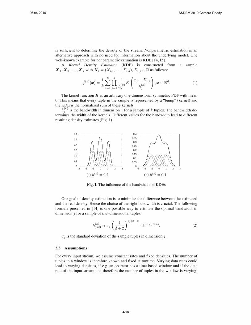
h(k)j is the bandwidth in dimension j for a sample of k tuples. The bandwidth de-

termines the width of the kernels. Different values for the bandwidth lead to differentresulting density estimates (Fig. 1).

0

0.1

0.2

0.3

0.4

0.5

0.6

-3 -2 -1 0 1 2 3

(a) h(k) = 0.2

0

0.05

0.1

0.15

0.2

0.25

0.3

0.35

0.4

-3 -2 -1 0 1 2 3

(b) h(k) = 0.4

Fig. 1. The influence of the bandwidth on KDEs

One goal of density estimation is to minimize the difference between the estimatedand the real density. Hence the choice of the right bandwidth is crucial. The followingformula presented in [14] is one possible way to estimate the optimal bandwidth indimension j for a sample of k d–dimensional tuples:

h(k)j,opt ≈ σj

(4

d+ 2

)1/(d+4)

· k−1/(d+4). (2)

σj is the standard deviation of the sample tuples in dimension j.

3.3 Assumptions

For every input stream, we assume constant rates and fixed densities. The number oftuples in a window is therefore known and fixed at runtime. Varying data rates couldlead to varying densities, if e.g. an operator has a time-based window and if the datarate of the input stream and therefore the number of tuples in the window is varying.


4/18

If rates or densities change in a relevant way during runtime, a recalculation might benecessary.

Our underlying model uses probability distributions over continuous values. Withlimited precision, it works well for discrete data streams, if there is a sufficiently highnumber of uniformly distributed distinct elements in the stream. We cannot supportnominal attributes like strings. Specific values are approximated by defining an interval;e.g. equi-joins are simulated by overlapping ranges. As grouping relies on finding tupleswith identical values in the grouping attributes, our approach does not support grouping.A definition of interval-based grouping is out of the scope of this paper.

4 Analytic Propagation

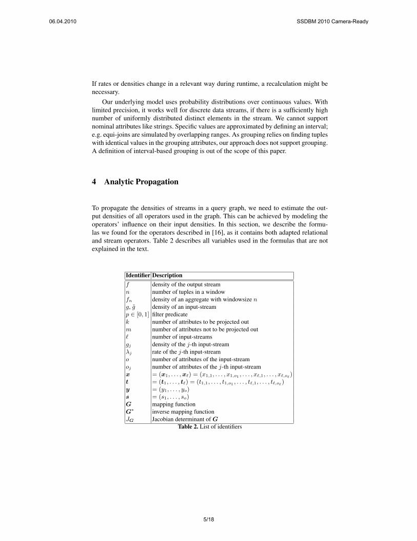
To propagate the densities of streams in a query graph, we need to estimate the out-put densities of all operators used in the graph. This can be achieved by modeling theoperators’ influence on their input densities. In this section, we describe the formu-las we found for the operators described in [16], as it contains both adapted relationaland stream operators. Table 2 describes all variables used in the formulas that are notexplained in the text.

Identifier Descriptionf density of the output streamn number of tuples in a windowfn density of an aggregate with windowsize ng, g density of an input-streamp ∈ [0, 1] filter predicatek number of attributes to be projected outm number of attributes not to be projected out` number of input-streamsgj density of the j-th input-streamλj rate of the j-th input-streamo number of attributes of the input-streamoj number of attributes of the j-th input-streamx = (x1, . . . ,x`) = (x1,1, . . . , x1,o1 , . . . , x`,1, . . . , x`,o`)t = (t1, . . . , t`) = (t1,1, . . . , t1,o1 , . . . , t`,1, . . . , t`,o`)y = (y1, . . . , yo)s = (s1, . . . , so)G mapping functionG∗ inverse mapping functionJG Jacobian determinant of G

Table 2. List of identifiers


5/18

4.1 Union

The Union operator has ` input streams and one output stream. All input streams havethe same schema, but they usually have different densities and input rates. Every tuplethat arrives on one input stream is immediately forwarded to the output stream. Hencethe output density is a weighted sum of the input streams’ densities.

The weight for input stream i is λi∑`j=1 λj

. The more tuples arrive on one input stream

the higher its weight. The weights are normalized to guarantee that the result is a den-sity. The output density is calculated as follows:

f(y) =1∑`j=1 λj

∑j=1

λjgj(y). (3)

4.2 Filter

A Filter is an operator with a predicate P , one input stream, and one output stream.A tuple is only forwarded to the output stream if it satisfies the Filter’s predicate. Thesupport of the output stream’s density is therefore the support of the input stream’sdensity minus the subset of Rn for which the predicate P is not satisfied. The selectivityof the Filter

∫g(s)p(s) ds is needed to normalize the resulting density.

A function p is defined as:

p(y) =

{1 if y satisfies the predicate P0 else .

The resulting density can therefore be described as follows:

f(y) =1∫

g(s)p(s) dsg(y)p(y). (4)

4.3 Join

The Join operator has ` input streams and one output stream. Each input stream mayhave a different schema and a different rate. A query defines a window for each inputstream. Join tests each possible combination of tuples in these windows if it matchesthe join predicate P and forwards it to the output stream, if it satisfies the predicate.The attribute value distribution of a tuple which is part of one of those combinationsis independent of the window sizes and the input streams’ rates. Hence the resultingdensity is basically a product density with a filter applied to it. The function p is likewisedefined as it was for the filter.

f(x) =1∫

p(t)∏`j=1 gj(tj) dt

p(x)∏j=1

gj(xj) (5)

If the predicate P is always satisfied, the Join would basically be a Cartesian productbetween the windows over the input streams. Then the resulting density could simply


6/18

be described as:

f(x) =∏j=1

gj(xj). (6)

Operator Output Density

Filter f(y) =1∫

g(s)p(s) dsg(y)p(y)

Join f(x) =1∫

p(t)∏`

j=1 gj(tj) dtp(x)

∏j=1

gj(xj)

Projection f(x1, . . . , xm) =

∫g(x1, . . . , xm, τ1, . . . , τk) dτ1 . . .dτk

Aggregate Sum fn(x) = (g ∗ . . . ∗ g)︸︷︷︸n times

(x)

Aggregate Avg fn(x) = n · (g ∗ . . . ∗ g)︸︷︷︸n times

(nx)

Aggregate Max fn(x) = ng(x)

(∫ x

−∞g(τ) dτ

)n−1

Aggregate Min fn(x) = ng(x)

(∫ ∞x

g(τ) dτ

)n−1

Aggregate Count fn(x) = δ(x− n)

Union f(y) =1∑`

j=1 λj

∑j=1

λjgj(y)

Map f(x) = g(G∗(x))1

|JG(G∗(x))|

Map (affine) f(x) = g(A−1(x− c))1

|det(A)| , G(x) = Ax+ c

BSort f(y) = g(y)

Resample f(y1,y2) = g1(y1) · g2(y2)Table 3. Operators’ output densities

4.4 Projection

A Projection operator removes certain attributes from each tuple that arrives on its sin-gle input stream. Therefore the resulting stream has a different schema. In the caseof data stream processing, only duplicate preserving projection is considered. Projec-tion could also rename the attributes in the schema, but this does not affect the outputstream’s density.

For the sake of simplicity we assume that the m+ k attributes are ordered in a waythat the last k attributes will be deleted by the Projection. If the input stream’s attribute


7/18

value distribution is g : Rm+k → R, the output stream’s distribution would be:

f(x1, . . . , xm) =

∫g(x1, . . . , xm, τ1, . . . , τk) dτ1 . . . dτk. (7)

4.5 Aggregate

The Aggregate operator applies an aggregate function to all tuples in a window overits single input stream. We assume that these tuples only have one attribute. All otherattributes are projected out as follows:

g(xj) =

∫· · ·∫g(x1, . . . , xo) dx1 . . . dxj−1 dxj+1 . . . dxo.

Because we assume the rate to be constant, the number of tuples in a window isknown, even for time based windows.

Sum The output density of the sum of n values is the convolution of the input densities.

fn(x) = (g ∗ . . . ∗ g)︸︷︷︸n times

(x) (8)

Average By means of the change of variables formula, the output density for the aver-age of n values can be derived from the formula for the sum of n values.

fn(x) = n · (g ∗ . . . ∗ g)︸︷︷︸n times

(nx) (9)

Maximum The distribution function of the maximum of n values is:

Fn(x) =

(∫ x

−∞g(τ) dτ

)n.

Hence the PDF of the output stream is:

fn(x) = F ′n(x) = ng(x)

(∫ x

−∞g(τ) dτ

)n−1. (10)

Minimum The density of the minimum of n values is as follows:

fn(x) = ng(x)

(∫ ∞x

g(τ) dτ

)n−1. (11)


8/18

Count Let δ be the Dirac delta function, with the property:∫ ∞−∞

δ(x) dx = 1.

The density of the count of n values can be described as:

fn(x) = δ(x− n) ={+∞, x = n

0, x 6= n. (12)

In reality, the rate is usually not constant but determined by the distribution of theinter-arrival times. Therefore the output density depends on the PDF of the inter-arrivaltimes.

4.6 Map

The Map operator applies a function G : Rm → Rm to every single input tuple x =(x1, . . . , xm) producing output tuples y = (y1, . . . , ym). If G fulfills the requirementsof the change of variables formula, the output density is:

f(x) = g(G∗(x))1

|JG(G∗(x))|. (13)

If G is an affine transformation G(x) = Ax + c then the output stream’s densitycan be described as:

f(x) = g(A−1(x− c))1

|det(A)|. (14)

4.7 BSort

The BSort operator approximately sorts its input stream by applying a certain numberof bubble-sort passes. Because the output tuples are the same as the input tuples butpossibly in a different order, the operator’s output density is the same as its input density.

f(y) = g(y) (15)

4.8 Resample

The Resample operator has two input streams and aligns tuples coming from the secondinput stream with tuples from the first input stream. To achieve this, the Resample op-erator interpolates tuples of the second input stream to match the time stamp of a tuplefrom the first input stream.

Under certain assumptions, a stream consisting of perfectly interpolated tuples hasthe same attribute value distribution as the original stream. These assumptions are man-ifold but out of the scope of this paper.

Let g1 be the density of the first input stream and g2 the density of the second inputstream. Assuming a perfect interpolation, the resulting density is:

f(y1,y2) = g1(y1) · g2(y2). (16)


9/18

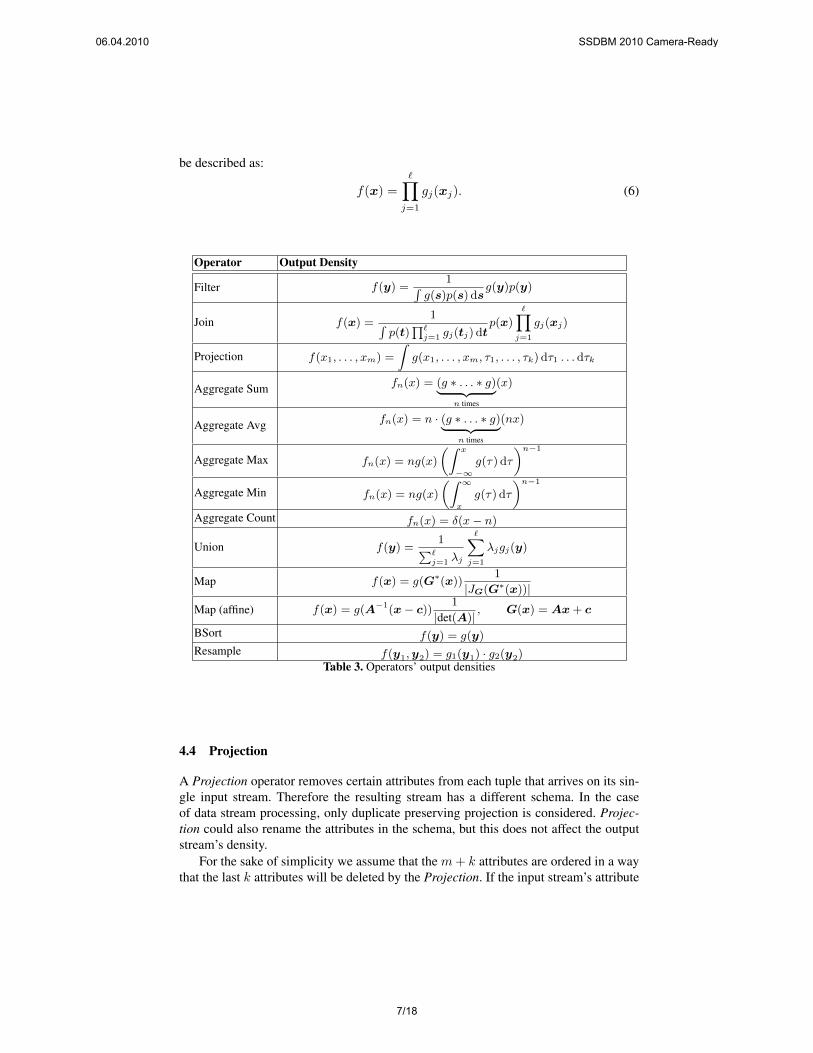
4.9 Summary

In this section, we have explained our formulas for the analytic estimation of probabilitydistributions for several operators. These include the most important stream operators(Filter, Join, Projection, Union, and Map) as well as several aggregates, the BSort, andthe Resample operator. For reference, the formulas are summarized in Table 3.

5 Numerical Propagation

In the previous section, we described an analytic method for estimating densities. Thisapproach relies on finding formulas that describe each operator’s output density. Thus, itis not applicable for operators for which no formulas are known (yet). This is a problemas there is currently no consensus about the basic set of data stream operators. Addi-tionally, some User-Defined Operators (UDOs) are hard or even impossible to model.

In order to overcome this problem, we developed a method for numerically estimat-ing the output densities of operators.

This method consists of two steps: In the first step (configuration phase), we build anumerical model that describes an operator instance’s behavior. As the model dependson the operator’s configuration (e.g. filter predicate), it is computed when the operatoris instantiated and its configuration is known. This model is independent of the actualinput distributions which need not be known at this time.

The second step (application phase) is performed when the query graph is instan-tiated. It combines knowledge of the actual input distributions with the model of theoperator in order to describe the output distributions.

The advantage of this two-step approach is that the computationally expensive modelbuilding needs to be performed only once for each operator instance. The second stephas to be done every time an operator graph is instantiated. During optimization, severalquery graphs may be instantiated for a single query. It is the optimizer’s duty to choosethe best one. Fortunately, the second step can be computed relatively quickly.

After outlining some requirements and limitations of this approach, we will describeboth steps in detail.

5.1 Requirements

In order to apply the numerical estimation, a number of requirements have to be ful-filled. These requirements are detailed below.

Determinism Obviously, operators have to act deterministically. An indeterministicoperator may behave differently between the test and the real execution, rendering thetest results worthless. Additionally, an operator’s output may only depend on its inputbut not on its state because it is not feasible to model all possible states. We modelwindows as additional input dimensions.

Continuity As an operator cannot be tested with all possible input values, we mustassume that small variations in the input values only lead to small variations in theoutput values. More formally, an operator has to be continuous on subsets of its domain.


10/18

Known Domain In order to test an operator with an uniform input distribution, thedomain of the input streams has to be known in advance as it is not possible to test withan uniform distribution on an infinite domain. This knowledge may be gained by testingand stored in the metadata catalog.

For operators that have intermediate streams as input, the domain of the intermediatestreams has to be known as well. We solve this problem by topologically ordering thequery graph and deriving the domain of the intermediate streams from the knowledgeabout input streams and intermediate operators. This requires the operator graph to beacyclic.

Independence Of Rates As we do not model the influence of rates on an operator’sbehavior, we require that an operator is independent of the rates of its input streams. Themost common rate-dependent operators are time-based windows. We sketch an idea forcoping with time-based windows in Sect. 5.4.

5.2 Test with Uniform Distribution (Configuration Phase)

In order to describe the influence of an operator on its output streams, it is tested withsynthetic inputs. This yields a model of an operator’s behavior. The model is built whenthe operator is deployed, as it depends on the configuration of the operator as well asknowledge of its input domains.

The operator is tested with k input values that are randomly and uniformly chosenfrom its input domains. The value of k has to be carefully chosen to balance accuracyversus memory requirements. Each input value is stored together with its correspondingoutput value. If a given input value does not produce any output, it is stored nevertheless,together with a flag that denotes that no output was produced. This will be required forselectivity estimation. Together the input and output values form the operator model.

5.3 Estimating Densities (Application Phase)

When the operator graph is instantiated, we measure the actual densities of input streamsand estimate the densities of intermediate streams. The input densities are then com-bined with the operator model in order to yield the actual output densities.

For each combination of input and output values in the model, we compute a weightwhich is based on the input densities. The estimated output density is a weighted sumof kernels based on the output values in the previously calculated operator model.

The weight of each kernel is given by the following equation:

gi = u(G∗(Xi)).

Here, u is the actual input density, G∗ is the operator’s inverse mapping function of theoperator model. Xi is an output value in the operator model.

As the integral over a density has to be 1, the weights have to be normalized. Thiscondition holds if the sum of all weights in (17) equals 1.

g∗i =gi∑kj=1 gj


11/18

Finally, we just have to apply a weighted version of (1) as suggested in [17]. Theoutput of this equation is the estimated output density.

f (k)(x) =k∑i=1

g∗i

d∏j=1

1

h(k)j

K

(xj −Xi,j

h(k)j

),x ∈ Rd (17)

The optimal bandwidths h(k)j can be estimated with (2) in Sect. 3.2.

Selectivity Estimation The selectivity of an operator can be easily derived from theavailable information. Remember that input values which produce no output are notexcluded from the operator model. Thus, after the weights of the kernels are known forthe actual input, the selectivity is just the ratio of the sum of weights for kernels withoutoutput and the sum of weights for all kernels.

5.4 Further Work

The approach described in this section may still be improved in numerous ways. Wesketch the two extensions which in our opinion promise the greatest benefits.

Compression The models for operators with high dimensions or large domains requirea large number of kernels for accurate results. This leads to high memory usage as wellas increased computational costs at runtime. One solution to this problem might becluster kernels [2].

The basic idea is to combine several kernels to a single one by means of clustering.For best results, the right choice of clusters is crucial. This choice largely depends onthe function that computes the distance between two kernels. It turns out that neither thedistance between input values di nor the distance between output values do is a goodchoice. The combination of these distances d =

√d2i + d2o however gives adequate

results. Some additional thought is required to determine which information has to bestored for each kernel. [2] discusses several possibilities.

Time-based Windows As in Sect. 4, windows are modeled as additional dimensions.This is not directly feasible for time-based windows, as their size is unknown whichleads to an unknown number of dimensions. It may however be possible to transforman operator in a way that the window size is set to a fixed maximum value. Then theactual window size depending on the rate is modeled as an additional parameter. Forthis approach, it is necessary to determine an upper bound for the window size.

5.5 Summary

The approach described in this section allows to estimate the value distributions for op-erators for which no analytic formula is known. If an analytic description of an operatoris available, it is preferred to the numerical approach. The numerical approach is how-ever more general and allows to model e.g. user defined operators. As both approacheshave their merits, they should be combined.


12/18

6 Synthesis

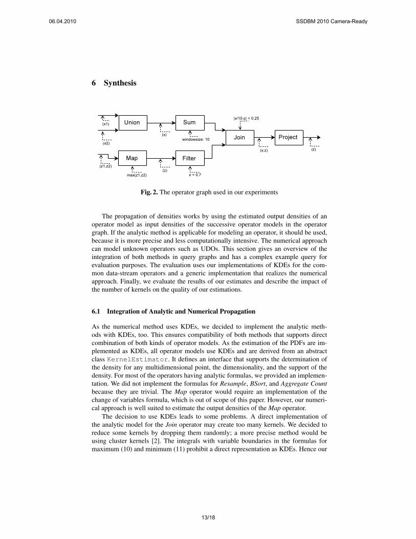
Fig. 2. The operator graph used in our experiments

The propagation of densities works by using the estimated output densities of anoperator model as input densities of the successive operator models in the operatorgraph. If the analytic method is applicable for modeling an operator, it should be used,because it is more precise and less computationally intensive. The numerical approachcan model unknown operators such as UDOs. This section gives an overview of theintegration of both methods in query graphs and has a complex example query forevaluation purposes. The evaluation uses our implementations of KDEs for the com-mon data-stream operators and a generic implementation that realizes the numericalapproach. Finally, we evaluate the results of our estimates and describe the impact ofthe number of kernels on the quality of our estimations.

6.1 Integration of Analytic and Numerical Propagation

As the numerical method uses KDEs, we decided to implement the analytic meth-ods with KDEs, too. This ensures compatibility of both methods that supports directcombination of both kinds of operator models. As the estimation of the PDFs are im-plemented as KDEs, all operator models use KDEs and are derived from an abstractclass KernelEstimator. It defines an interface that supports the determination ofthe density for any multidimensional point, the dimensionality, and the support of thedensity. For most of the operators having analytic formulas, we provided an implemen-tation. We did not implement the formulas for Resample, BSort, and Aggregate Countbecause they are trivial. The Map operator would require an implementation of thechange of variables formula, which is out of scope of this paper. However, our numeri-cal approach is well suited to estimate the output densities of the Map operator.

The decision to use KDEs leads to some problems. A direct implementation ofthe analytic model for the Join operator may create too many kernels. We decided toreduce some kernels by dropping them randomly; a more precise method would beusing cluster kernels [2]. The integrals with variable boundaries in the formulas formaximum (10) and minimum (11) prohibit a direct representation as KDEs. Hence our


13/18

1 stream S1(x1 float)2 stream S2(x2 float)3 stream S3(z1 float,z2 float)4

5 UnionStream(x):6 S1 UNION S27

8 AggStream(x):9 SELECT SUM(x) FROM UnionStream[rows 10]

10

11 MapStream(z):12 SELECT MAX(z1,z2) FROM S313

14 FilterStream(z):15 SELECT z FROM MapStream WHERE z < 0.716

17 JoinStream(x,z):18 SELECT x,z FROM FilterStream[rows 10],19 AggStream[rows 10]20 WHERE x/10-z < 0.2521 AND x/10-z > -0.2522

23 ProjectStream(z):24 SELECT z FROM JoinStream

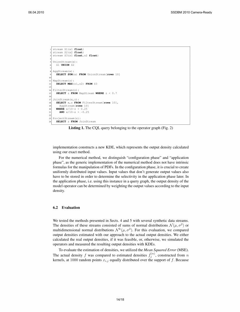
Listing 1. The CQL query belonging to the operator graph (Fig. 2)

implementation constructs a new KDE, which represents the output density calculatedusing our exact method.

For the numerical method, we distinguish “configuration phase” and “applicationphase”, as the generic implementation of the numerical method does not have intrinsicformulas for the manipulation of PDFs. In the configuration phase, it is crucial to createuniformly distributed input values. Input values that don’t generate output values alsohave to be stored in order to determine the selectivity in the application phase later. Inthe application phase, i.e. using this instance in a query graph, the output density of themodel operator can be determined by weighting the output values according to the inputdensity.

6.2 Evaluation

We tested the methods presented in Sects. 4 and 5 with several synthetic data streams.The densities of these streams consisted of sums of normal distributions N (µ, σ2) ormultidimensional normal distributions N k(µ, σ2). For this evaluation, we comparedoutput densities estimated with our approach to the actual output densities. We eithercalculated the real output densities, if it was feasible, or, otherwise, we simulated theoperators and measured the resulting output densities with KDEs.

To evaluate the estimation of densities, we utilized the Mean Squared Error (MSE).The actual density f was compared to estimated densities f (n)j , constructed from nkernels, at 1000 random points xi,j equally distributed over the support of f . Because


14/18

0

1

2

3

4

5

6

7

0 0.1 0.2 0.3 0.4 0.5 0.6

dens

ity

value

actual densityestimation with bandwidth h

estimation with bandwidth 1/2*hestimation with bandwidth 1/4*h

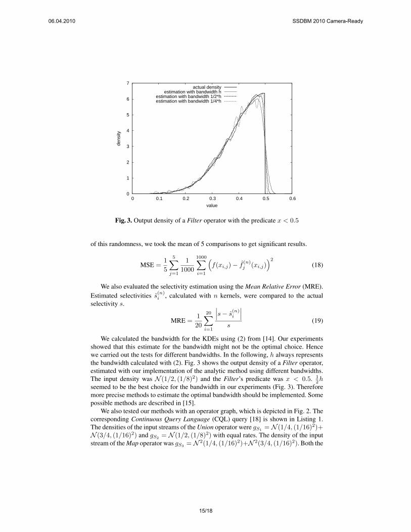
Fig. 3. Output density of a Filter operator with the predicate x < 0.5

of this randomness, we took the mean of 5 comparisons to get significant results.

MSE =1

5

5∑j=1

1

1000

1000∑i=1

(f(xi,j)− f (n)j (xi,j)

)2(18)

We also evaluated the selectivity estimation using the Mean Relative Error (MRE).Estimated selectivities s(n)i , calculated with n kernels, were compared to the actualselectivity s.

MRE =1

20

20∑i=1

∣∣∣s− s(n)i

∣∣∣s

(19)

We calculated the bandwidth for the KDEs using (2) from [14]. Our experimentsshowed that this estimate for the bandwidth might not be the optimal choice. Hencewe carried out the tests for different bandwidths. In the following, h always representsthe bandwidth calculated with (2). Fig. 3 shows the output density of a Filter operator,estimated with our implementation of the analytic method using different bandwidths.The input density was N (1/2, (1/8)2) and the Filter’s predicate was x < 0.5. 1

2hseemed to be the best choice for the bandwidth in our experiments (Fig. 3). Thereforemore precise methods to estimate the optimal bandwidth should be implemented. Somepossible methods are described in [15].

We also tested our methods with an operator graph, which is depicted in Fig. 2. Thecorresponding Continuous Query Language (CQL) query [18] is shown in Listing 1.The densities of the input streams of the Union operator were gS1

= N (1/4, (1/16)2)+N (3/4, (1/16)2) and gS2

= N (1/2, (1/8)2) with equal rates. The density of the inputstream of the Map operator was gS3

= N 2(1/4, (1/16)2)+N 2(3/4, (1/16)2). Both the


15/18

0

1

2

3

4

5

6

7

0 0.1 0.2 0.3 0.4 0.5 0.6 0.7 0.8

dens

ity

value

measured densityestimated density

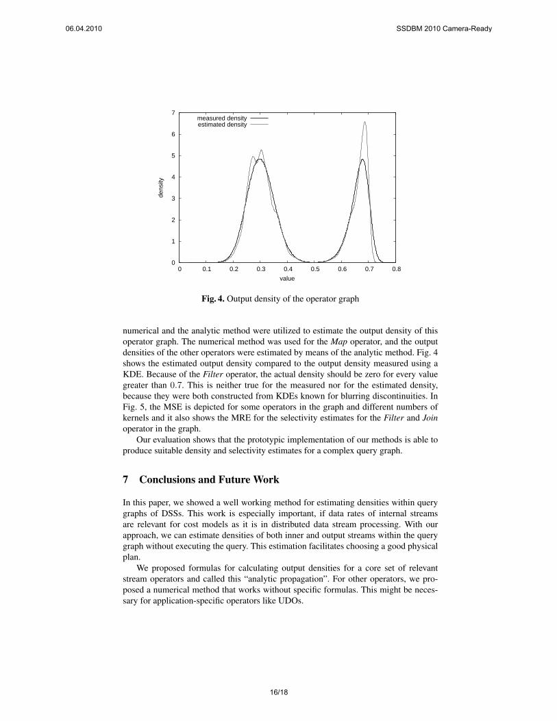
Fig. 4. Output density of the operator graph

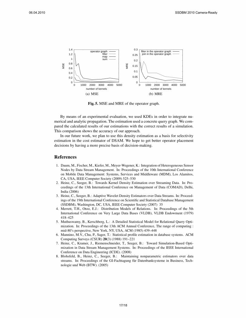
numerical and the analytic method were utilized to estimate the output density of thisoperator graph. The numerical method was used for the Map operator, and the outputdensities of the other operators were estimated by means of the analytic method. Fig. 4shows the estimated output density compared to the output density measured using aKDE. Because of the Filter operator, the actual density should be zero for every valuegreater than 0.7. This is neither true for the measured nor for the estimated density,because they were both constructed from KDEs known for blurring discontinuities. InFig. 5, the MSE is depicted for some operators in the graph and different numbers ofkernels and it also shows the MRE for the selectivity estimates for the Filter and Joinoperator in the graph.

Our evaluation shows that the prototypic implementation of our methods is able toproduce suitable density and selectivity estimates for a complex query graph.

7 Conclusions and Future Work

In this paper, we showed a well working method for estimating densities within querygraphs of DSSs. This work is especially important, if data rates of internal streamsare relevant for cost models as it is in distributed data stream processing. With ourapproach, we can estimate densities of both inner and output streams within the querygraph without executing the query. This estimation facilitates choosing a good physicalplan.

We proposed formulas for calculating output densities for a core set of relevantstream operators and called this “analytic propagation”. For other operators, we pro-posed a numerical method that works without specific formulas. This might be neces-sary for application-specific operators like UDOs.


16/18

0

0.2

0.4

0.6

0.8

1

1.2

1.4

0 1000 2000 3000 4000 5000

MS

E

number of kernels

operator graphfiltermapsum

(a) MSE

0

0.05

0.1

0.15

0.2

0.25

0.3

0 1000 2000 3000 4000 5000

MR

E

number of kernels

filter in the operator graphjoin in the operator graph

(b) MRE

Fig. 5. MSE and MRE of the operator graph.

By means of an experimental evaluation, we used KDEs in order to integrate nu-merical and analytic propagation. The estimation used a concrete query graph. We com-pared the calculated results of our estimations with the correct results of a simulation.This comparison shows the accuracy of our approach.

In our future work, we plan to use this density estimation as a basis for selectivityestimation in the cost estimator of DSAM. We hope to get better operator placementdecisions by having a more precise basis of decision-making.

References

1. Daum, M., Fischer, M., Kiefer, M., Meyer-Wegener, K.: Integration of Heterogeneous SensorNodes by Data Stream Management. In: Proceedings of the 10th International Conferenceon Mobile Data Management: Systems, Services and Middleware (MDM), Los Alamitos,CA, USA, IEEE Computer Society (2009) 525–530

2. Heinz, C., Seeger, B.: Towards Kernel Density Estimation over Streaming Data. In: Pro-ceedings of the 13th International Conference on Management of Data (COMAD), Delhi,India (2006)

3. Heinz, C., Seeger, B.: Adaptive Wavelet Density Estimators over Data Streams. In: Proceed-ings of the 19th International Conference on Scientific and Statistical Database Management(SSDBM), Washington, DC, USA, IEEE Computer Society (2007) 35

4. Merrett, T.H., Otoo, E.J.: Distribution Models of Relations. In: Proceedings of the 5thInternational Conference on Very Large Data Bases (VLDB), VLDB Endowment (1979)418–425

5. Muthuswamy, B., Kerschberg, L.: A Detailed Statistical Model for Relational Query Opti-mization. In: Proceedings of the 13th ACM Annual Conference, The range of computing :mid-80’s perspective, New York, NY, USA, ACM (1985) 439–448

6. Mannino, M.V., Chu, P., Sager, T.: Statistical profile estimation in database systems. ACMComputing Surveys (CSUR) 20(3) (1988) 191–221

7. Heinz, C., Kramer, J., Riemenschneider, T., Seeger, B.: Toward Simulation-Based Opti-mization in Data Stream Management Systems. In: Proceedings of the IEEE InternationalConference on Data Engineering (ICDE). (2008)

8. Blohsfeld, B., Heinz, C., Seeger, B.: Maintaining nonparametric estimators over datastreams. In: Proceedings of the GI-Fachtagung fur Datenbanksysteme in Business, Tech-nologie und Web (BTW). (2005)


17/18

9. Gunopulos, D., Kollios, G., Tsotras, J., Domeniconi, C.: Selectivity estimators for multidi-mensional range queries over real attributes. The International Journal on Very Large DataBases (VLDBJ) 14(2) (2005) 137–154

10. Viglas, S.D., Naughton, J.F.: Rate-Based Query Optimization for Streaming InformationSources. In: Proceedings of the 2002 ACM SIGMOD International Conference on Manage-ment of Data (SIGMOD), ACM Press New York, NY, USA (2002) 37–48

11. Meyerhofer, M.: Messung und Verwaltung von Softwarekomponenten fur die Perfor-mancevorhersage. PhD thesis, University of Erlangen-Nuremberg (2007)

12. Hamlet, D., Mason, D., Woit, D.: Properties of Software Systems Synthesized from Com-ponents. In: Component-Based Software Development: Case Studies. World Scientific Pub-lishing Company (2004) 129–159

13. Heinz, C.: Density Estimation over Data Streams. PhD thesis, University of Marburg (2007)14. Silverman, B.: Density Estimation for Statistics and Data Analysis. Monographs on Statistics

and Applied Probability, London: Chapman and Hall (1986)15. Scott, D.W.: Multivariate Density Estimation. Wiley-Interscience (1992)16. Abadi, D.J., Carney, D., Cetintemel, U., Cherniack, M., Convey, C., Lee, S., Stonebraker, M.,

Tatbul, N., Zdonik, S.: Aurora: a new model and architecture for data stream management.The International Journal on Very Large Data Bases (VLDBJ) 12(2) (2003) 120–139

17. Zhou, A., Cai, Z., Wei, L., Qian, W.: M-Kernel Merging: Towards Density Estimation overData Streams. In: Proceedings of the 8th International Conference on Database Systems forAdvanced Applications (DASFAA), Washington, DC, USA, IEEE Computer Society (2003)285–292

18. Arasu, A., Babu, S., Widom, J.: The CQL continuous query language: semantic foundationsand query execution. The International Journal on Very Large Data Bases (VLDBJ) 15(2)(2006) 121–142


18/18

propagation of densities of streaming data within query graphs · propagation of densities of...

Documents