programming languages capturing complexity classesfolk.uio.no/larsk/njc.pdf · programming...

Nordic Journal of Computing

Programming Languages Capturing Complexity Classes

LARS KRISTIANSENOslo University College, Faculty of Engineering

PO Box 4, St. Olavs Plass, NO-0130 Oslo, NorwayDepartment of Mathematics, University of OsloPO Box 1053, Blindern, NO-0316 Oslo, Norway

[email protected]

PAUL J. VODAInstitute of Informatics, Comenius University Bratislava

Mlynska dolina, 842 15 Bratislava, [email protected]

Abstract. We investigate an imperative and a functional programming language. Thecomputational power of fragments of these languages inducetwo hierarchies of com-plexity classes. Our first main theorem says that these hierarchies match, level by level,a complexity-theoretic alternating space-time hierarchyknown from the literature. Oursecond main theorems says that a slightly different complexity-theoretic hierarchy (theGoerdt-Seidl hierarchy) also can be captured by hierarchies induced by fragments of theprogramming languages. Well known complexity classes like, , , ,etc., occur in the hierarchies.

ACM CCS Categories and Subject Descriptors: F.4.1, F.1.3

Key words: Imperative and functional programming languages, typedλ-calculi, highertypes, complexity classes, computational complexity.

1. Introduction

In this paper we relate the computational power of natural fragments of pure andsimple programming languages to complexity classes definedby Turing machinesand explicit resource bounds. The elements of the languageswe investigate con-stitute an essential core of many real-life programming languages. We study afunctional programming language which is simply the typedλ-calculus extendedwith recursors and numerals. The typedλ-calculus with its syntax and semanticsis an essential part of languages like Lisp, ML, Haskell, etc. Further, we study animperative language with syntax and semantics reminiscentof e.g. Pascal and C.Higher types are essential constituents in both languages.

We think the results presented in this paper are interestingfor several reasons.(1)Complexity theory and programming language theory:We subscribe to the thesisthat complexity and programming language theories have much to offer each other,in both directions [Jones 1997]. Our results somewhat bridge the gap between thetwo areas. Moreover, they also provide some evidence for thethesis by giving ananalysis of the expressive power of elements of imperative languages versus the

Received February 3, 2005; accepted June 22, 2005.

2 L. KRISTIANSEN, P. J. VODA

expressive power of elements of functional languages. Thisanalysis is founded oncomplexity theory.(2) The naturalness of the complexity classes:During the lastthree or four decades researchers have provided so called resource-free and intrin-sic characterizations of the complexity classes, e.g. the seminal papers of Cobham[1965], Fagin [1974], Bellantoni and Cook [1992]. One of themotivations is toshow that the complexity classes, defined by a particular machine model and ex-plicit resource bounds, are natural entities, and that complexity theory is a robustand mathematically interesting field. Our theorems provideyet another argumentin favor of the naturalness of the complexity classes.(3) Open problems in com-plexity theory:The characterizations of the complexity classes given paper mightshed some light upon some of the many open questions regarding the relationshipbetween these classes.(4) Goerdt and Seidl’s work:Some work of Goerdt andSeidl’s is less known than it deserves to be. We remedy the situation by payingattention to the results and techniques from Goerdt and Seidl [1990] and Goerdt[1992]. (5) Pedagogical value:Many scientists and researchers familiar with pro-gramming languages and programming theory, are not familiar with complexitytheory. This paper might be informative and enlightening tosuch an audience ande.g. help them to acquire a better understanding of open problems in complexitytheory.

This paper is organized as follows. In Section 2 we define the programminglanguages and state the first of two main theorems. The three subsequent sectionsgive the proof this theorem. These sections are occasionally very technical, andsome readers might want to skip them and go straight ahead to Section 6 wherewe state the second main theorem and make a summary. (The proofs of the twotheorem are uniform, and hence, we will not give a proof of thesecond theorem.)In the final section we discuss some related research.

The results in this paper are generalizations and refinements of the results pub-lished in Kristiansen and Voda [2003a, 2003b].

2. The Programming Languages and the Main Result

2.1 Turing Machines and the Alternating Space-Time Hierarchy

We will assume that the read is familiar with Turing machinesand basic com-plexity theory. For more on the subject see e.g. Odifreddi [1999] or Lewis andPapadimitriou [1998].

D 1. A Turing machine Mdecidesa problem A when M on input x∈ Nhalts in a distinguished accept state if x∈ A, and in a distinguished reject state ifx < A. The input x∈ N should be represented in binary on the Turing machine’sinput tape. We will use|x| to denote the length of the standard binary representationof the natural number x. For i∈ N, we define 2i ( 2i ) to be the set of

problem decidable by a deterministic Turing machine working in time (space)2c|x|i

for some fixed c∈ N. (The notation2xi is as usual defined by2x

0 = x and2xi+1 = 22x

i )

PROGRAMMING LANGUAGES . . . 3

It is trivial that 2i ⊆ 2i and 2i ⊆ 2i+1, and thus, we haveanalternating space-time hierarchy

20 ⊆ 21 ⊆ 21 ⊆ 22 ⊆ 22 ⊆ 23 ⊆ . . . .

The three classes at the bottom of the hierarchy are called respectively, ,and in the literature. It is well known, and quite obvious, that 2i ⊂ 2i+1 and 2i ⊂ 2i+1 hold for anyi ∈ N. Thus, at least one of the twoinclusions

2i ⊆ 2i ⊆ 2i+1

must be strict, but it is not known which one(s). Further, at least one of the twoinclusions

2i ⊆ 2i ⊆ 2i+1

has to be strict, but it is not known which one(s). In particular, no one knows if is strictly included in, and no one knows if is strictly included in. These notorious open problems are again closely related tothe even morenotorious problems of complexity theory, e.g. is strictly included in; is strictly included in? Complexity theorists in general, and the authors inparticular, suspect all these inclusions to be strict, and it is a bit of a mystery thatit should be so hard to find proofs. A further study of the two alternating space-time hierarchies might shed some light on these and similar pivotal questions ofcomplexity theory (e.g. if we could prove forsome n∈ N that 2n , 2n+1it follows that , and , ).

2.2 Numbers and Types

D 2. We will use small Greek letters, with or without decorations, to de-notetypes. Thetypesare defined recursively:◦ 0 is a type

◦ σ→ τ is a type ifσ andτ are types

◦ σ × τ is a type ifσ andτ are types.We useσ,σ′ → σ′′ as alternative notation forσ → (σ′ → σ′′). We interpretσ→ σ′ → σ′′ by associating parentheses to the right, i.e. asσ→ (σ′ → σ′′). Wesay a typeσ is of level n whenlv(σ) = n where◦ lv(0) = 0

◦ lv(σ→ τ) = max(lv(σ) + 1, lv(τ))

◦ lv(σ × τ) = max(lv(σ), lv(τ)).We define thecardinality of typeσ at baseb, written |σ|b, by recursion on thestructure ofσ: (i) |0|b = b, (ii) |ρ→ τ|b = |τ|

|ρ|bb , and (iii) |ρ × τ|b = |ρ|b × |τ|b.

L 1. For any m, k ∈ N there exists a typeσ of level m such that2k|x|m+1 < |σ|x

for all but finitely many values of x.


P. First we prove by induction onm that for every polynomialp there existsa typeσ of levelmsuch that 2p(x)

m < |σ|x for all but finitely many values ofx. Casem = 0. Let 00

= 0 and0 j+1= 0 × 0 j . Thenp(x) < |0 j |x holds for all but finitely

many values ofx when j is sufficiently large. Step: Assume|σ|x > 2p(x)m where

lv(σ) = m. Then, we have 2p(x)m+1 = 2(2p(x)

m ) < 2|σ|x < (|0|x)|σ|x = |σ → 0|x for allbut finitely many values ofx. Further, lv(σ→ 0) = lv(σ) + 1. The lemma followssince for everyk ∈ N there exists polynomialp such that 2k|x| < p(x). �

L 2. For every typeσ of level k there exists a polynomial p such that2p(x)k >

|σ|x, and hence, there also exists c∈ N such that2c|x|k+1 > |σ|x.

P. We use induction on the structure ofσ. The caseσ = 0 is trivial. Assumeσ = ρ → τ. Then we have lv(ρ) ≤ n − 1 and lv(τ) ≤ n, and the inductionhypothesis yields polynomialsq and r such that 2q(x)

n−1 > |ρ|x and 2r(x)n > |τ|x. We

have|σ|x = |τ||ρ|xx < (2r(x)

n )2q(x)n−1 = 2(2r(x)

n−1×2q(x)n−1) ≤ 2r(x)+q(x)

n and the lemma holds whenp = r + q. (For any polynomialp(x) there existsc ∈ N such that 2c|x| > p(x).) �

D 3. The natural number a is anumber of typeσ at baseb, written a:σb,iff a < |σ|b. Let a: (σ→ τ)b. Then a can be viewed as a|σ|b digit number in base|τ|b, and thus, a can be uniquely written in the form

v0 + v1|τ|1b + · · · + vk|τ|

kb

where k= |σ|b−1 and vj :τb for j ∈ {0, . . . , k}. We call v0, . . . , vk thedigits in a, andfor any i:σb, we denote the i’th digit in a by a[i]b, i.e. a[i]b = vi . Furthermore, forany i:σb and w:τb, let a[i := w]b denote the number which is the result of settingthe i’th digit in a to w. (Note that a[i := w]b is a number of typeσ at base b.) Thenotation a[i1, . . . , in]b, where n≥ 1, abbreviates((a[i1]b)[i2]b) . . .)[in]b. Further,let

a[i1, . . . , in+1 := w]bdef= a[i1, . . . , in := a[i1, . . . , in]b[in+1 := w]b]b

for n ≥ 1. Thus, a[i1, . . . , in := w]b is the number which is the results of setting thesub-digit a[i1, . . . , in]b in a to w.

2.3 The Imperative Programming Language and theI-Hierarchy

We will use informal Hoare-like sentences to specify or reason about imperativeprograms, that is, we will use the notation{A} P {B}, the meaning being that ifthe condition given by the sentenceA is fulfilled beforeP is executed, then thecondition given by the sentenceB is fulfilled after the execution ofP. For example,{X = x, Y = y}P {X = x′, Y = y′} reads asif the values x and y are held by thevariablesX andY, respectively, before the execution ofP, then the values x′ andy′ are held byX andY after the execution ofP. We use typewriter style uppercaseand lowercase letters, with or without subscripts, to denote respectively programvariables and terms. Occasionally we indicate the type of a variable or a term by a


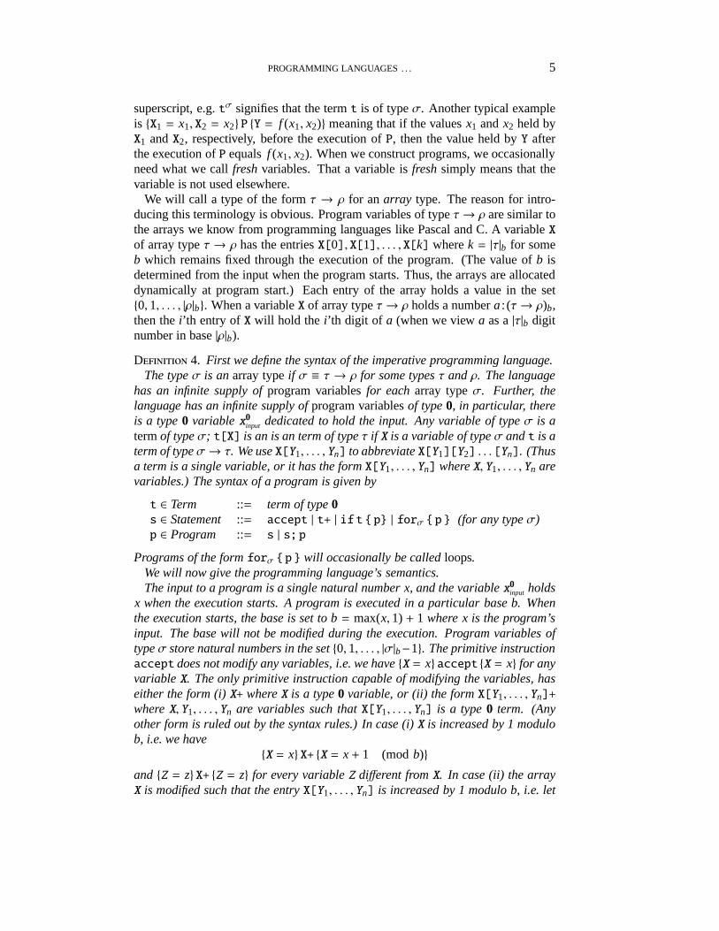
superscript, e.g.tσ signifies that the termt is of typeσ. Another typical exampleis {X1 = x1, X2 = x2} P {Y = f (x1, x2)} meaning that if the valuesx1 andx2 held byX1 andX2, respectively, before the execution ofP, then the value held byY afterthe execution ofP equalsf (x1, x2). When we construct programs, we occasionallyneed what we callfreshvariables. That a variable isfreshsimply means that thevariable is not used elsewhere.

We will call a type of the formτ → ρ for anarray type. The reason for intro-ducing this terminology is obvious. Program variables of typeτ→ ρ are similar tothe arrays we know from programming languages like Pascal and C. A variableXof array typeτ → ρ has the entriesX[0], X[1], . . . , X[k] wherek = |τ|b for someb which remains fixed through the execution of the program. (The value ofb isdetermined from the input when the program starts. Thus, thearrays are allocateddynamically at program start.) Each entry of the array holdsa value in the set{0, 1, . . . , |ρ|b}. When a variableX of array typeτ→ ρ holds a numbera: (τ→ ρ)b,then thei’th entry of X will hold the i’th digit of a (when we viewa as a|τ|b digitnumber in base|ρ|b).

D 4. First we define the syntax of the imperative programming language.The typeσ is anarray typeif σ ≡ τ → ρ for some typesτ andρ. The language

has an infinite supply ofprogram variablesfor eacharray typeσ. Further, thelanguage has an infinite supply ofprogram variablesof type0, in particular, thereis a type0 variable x0

input dedicated to hold the input. Any variable of typeσ is atermof typeσ; t[X] is an is an term of typeτ if X is a variable of typeσ andt is aterm of typeσ→ τ. We useX[Y1, . . . , Yn] to abbreviateX[Y1][Y2] . . . [Yn]. (Thusa term is a single variable, or it has the formX[Y1, . . . , Yn] whereX, Y1, . . . , Yn arevariables.) The syntax of a program is given by

t ∈ Term ::= term of type0s ∈ Statement ::= accept | t+ | if t { p} | forσ { p } (for any typeσ)p ∈ Program ::= s | s; p

Programs of the formforσ { p } will occasionally be calledloops.We will now give the programming language’s semantics.The input to a program is a single natural number x, and the variable x0

input holdsx when the execution starts. A program is executed in a particular base b. Whenthe execution starts, the base is set to b= max(x, 1) + 1 where x is the program’sinput. The base will not be modified during the execution. Program variables oftypeσ store natural numbers in the set{0, 1, . . . , |σ|b−1}. The primitive instructionaccept does not modify any variables, i.e. we have{X = x} accept {X = x} for anyvariableX. The only primitive instruction capable of modifying the variables, haseither the form (i)X+ whereX is a type0 variable, or (ii) the formX[Y1, . . . , Yn]+

whereX, Y1, . . . , Yn are variables such thatX[Y1, . . . , Yn] is a type0 term. (Anyother form is ruled out by the syntax rules.) In case (i)X is increased by 1 modulob, i.e. we have

{X = x} X+ {X = x+ 1 (modb)}

and {Z = z} X+ {Z = z} for every variableZ different fromX. In case (ii) the arrayX is modified such that the entryX[Y1, . . . , Yn] is increased by 1 modulo b, i.e. let


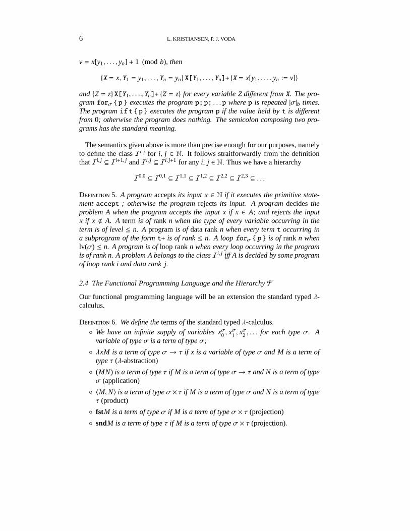
v = x[y1, . . . , yn] + 1 (modb), then

{X = x, Y1 = y1, . . . , Yn = yn} X[Y1, . . . , Yn]+ {X = x[y1, . . . , yn := v]}

and {Z = z} X[Y1, . . . , Yn]+ {Z = z} for every variableZ different fromX. The pro-gramforσ { p } executes the programp;p; . . . p wherep is repeated|σ|b times.The programift { p } executes the programp if the value held byt is differentfrom 0; otherwise the program does nothing. The semicolon composing two pro-grams has the standard meaning.

The semantics given above is more than precise enough for ourpurposes, namelyto define the classIi, j for i, j ∈ N. It follows straitforwardly from the definitionthatIi, j ⊆ Ii+1, j andIi, j ⊆ Ii, j+1 for any i, j ∈ N. Thus we have a hierarchy

I0,0 ⊆ I0,1 ⊆ I1,1 ⊆ I1,2 ⊆ I2,2 ⊆ I2,3 ⊆ . . .

D 5. A programacceptsits input x∈ N if it executes the primitive state-mentaccept ; otherwise the programrejectsits input. A programdecidestheproblem A when the program accepts the input x if x∈ A; and rejects the inputx if x < A. A term is of rank n when the type of every variable occurring in theterm is of level≤ n. A programis of data rankn when every termt occurring ina subprogram of the formt+ is of rank≤ n. A loopforσ { p } is of rankn whenlv(σ) ≤ n. A program is ofloop rankn when every loop occurring in the programis of rank n. A problem A belongs to the classIi, j iff A is decided by some programof loop rank i and data rank j.

2.4 The Functional Programming Language and the HierarchyF

Our functional programming language will be an extension the standard typedλ-calculus.

D 6. We define thetermsof the standard typedλ-calculus.◦ We have an infinite supply of variables xσ0 , x

σ1 , x

σ2 , . . . for each typeσ. A

variable of typeσ is a term of typeσ;

◦ λxM is a term of typeσ → τ if x is a variable of typeσ and M is a term oftypeτ (λ-abstraction)

◦ (MN) is a term of typeτ if M is a term of typeσ→ τ and N is a term of typeσ (application)

◦ 〈M,N〉 is a term of typeσ× τ if M is a term of typeσ and N is a term of typeτ (product)

◦ fstM is a term of typeσ if M is a term of typeσ × τ (projection)

◦ sndM is a term of typeτ if M is a term of typeσ × τ (projection).


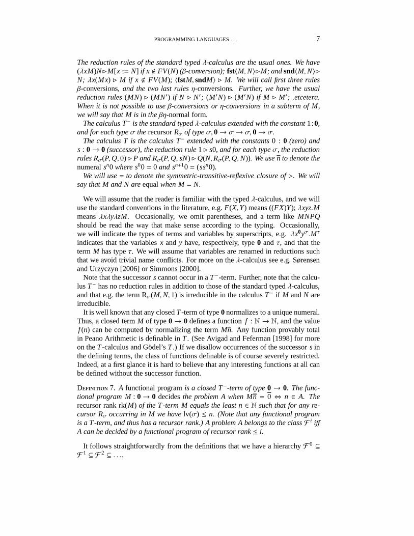
The reduction rules of the standard typedλ-calculus are the usual ones. We have(λxM)N⊲M[x := N] if x < FV(N) (β-conversion);fst〈M,N〉⊲M; andsnd〈M,N〉⊲N; λx(Mx) ⊲ M if x < FV(M); 〈fstM, sndM〉 ⊲ M. We will call first three rulesβ-conversions, and the two last rulesη-conversions. Further, we have the usualreduction rules(MN) ⊲ (MN′) if N ⊲ N′; (M′N) ⊲ (M′N) if M ⊲ M′; .etcetera.When it is not possible to useβ-conversions orη-conversions in a subterm of M,we will say that M is in theβη-normal form.

The calculus T− is the standard typedλ-calculus extended with the constant1:0,and for each typeσ therecursorRσ of typeσ, 0→ σ→ σ, 0→ σ.

The calculus T is the calculus T− extended with the constants0 : 0 (zero) ands : 0→ 0 (successor), the reduction rule1⊲ s0, and for each typeσ, the reductionrules Rσ(P,Q, 0)⊲P and Rσ(P,Q, sN)⊲Q(N,Rσ(P,Q,N)). We usen to denote thenumeralsn0 where s00 = 0 and sn+10 = (ssn0).

We will use= to denote the symmetric-transitive-reflexive closure of⊲. We willsay that M and N areequalwhen M= N.

We will assume that the reader is familiar with the typedλ-calculus, and we willuse the standard conventions in the literature, e.g.F(X,Y) means ((FX)Y); λxyz.MmeansλxλyλzM. Occasionally, we omit parentheses, and a term likeMNPQshould be read the way that make sense according to the typing. Occasionally,we will indicate the types of terms and variables by superscripts, e.g. λx0yσ.Mτ

indicates that the variablesx andy have, respectively, type0 andτ, and that theterm M has typeτ. We will assume that variables are renamed in reductions suchthat we avoid trivial name conflicts. For more on theλ-calculus see e.g. Sørensenand Urzyczyn [2006] or Simmons [2000].

Note that the successorscannot occur in aT−-term. Further, note that the calcu-lusT− has no reduction rules in addition to those of the standard typedλ-calculus,and that e.g. the term Rσ(M,N, 1) is irreducible in the calculusT− if M andN areirreducible.

It is well known that any closedT-term of type0 normalizes to a unique numeral.Thus, a closed termM of type0 → 0 defines a functionf : N → N, and the valuef (n) can be computed by normalizing the termMn. Any function provably totalin Peano Arithmetic is definable inT. (See Avigad and Feferman [1998] for moreon theT-calculus and Godel’sT.) If we disallow occurrences of the successors inthe defining terms, the class of functions definable is of course severely restricted.Indeed, at a first glance it is hard to believe that any interesting functions at all canbe defined without the successor function.

D 7. A functional programis a closed T−-term of type0 → 0. The func-tional program M: 0→ 0 decidesthe problem A when Mn = 0 ⇔ n ∈ A. Therecursor rank rk(M) of the T-term M equals the least n∈ N such that for any re-cursor Rσ occurring in M we havelv(σ) ≤ n. (Note that any functional programis a T-term, and thus has a recursor rank.) A problem A belongsto the classF i iffA can be decided by a functional program of recursor rank≤ i.

It follows straightforwardly from the definitions that we have a hierarchyF 0 ⊆

F 1 ⊆ F 2 ⊆ . . ..


2.5 The First Main Theorem

We are ready to state the first main theorem.

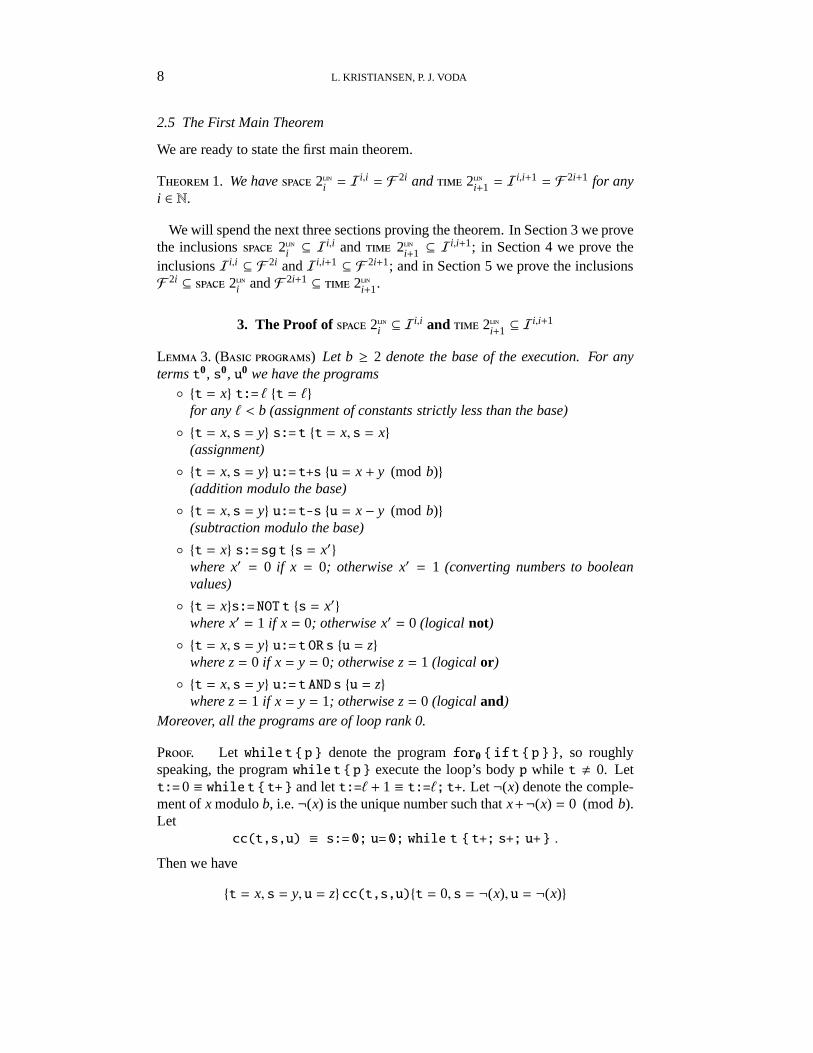
T 1. We have 2i = Ii,i= F 2i and 2i+1 = I

i,i+1= F 2i+1 for any

i ∈ N.

We will spend the next three sections proving the theorem. InSection 3 we provethe inclusions 2i ⊆ I

i,i and 2i+1 ⊆ Ii,i+1; in Section 4 we prove the

inclusionsIi,i ⊆ F 2i andIi,i+1 ⊆ F 2i+1; and in Section 5 we prove the inclusionsF 2i ⊆ 2i andF 2i+1 ⊆ 2i+1.

3. The Proof of 2i ⊆ Ii,i and 2i+1 ⊆ I

i,i+1

L 3. (B ) Let b ≥ 2 denote the base of the execution. For anytermst0, s0, u0 we have the programs◦ {t = x} t:= ℓ {t = ℓ}

for anyℓ < b (assignment of constants strictly less than the base)

◦ {t = x, s = y} s:=t {t = x, s = x}(assignment)

◦ {t = x, s = y} u:=t+s {u = x+ y (mod b)}(addition modulo the base)

◦ {t = x, s = y} u:=t-s {u = x− y (mod b)}(subtraction modulo the base)

◦ {t = x} s:= sgt {s = x′}where x′ = 0 if x = 0; otherwise x′ = 1 (converting numbers to booleanvalues)

◦ {t = x}s:=NOT t {s = x′}where x′ = 1 if x = 0; otherwise x′ = 0 (logical not)

◦ {t = x, s = y} u:=t OR s {u = z}where z= 0 if x = y = 0; otherwise z= 1 (logical or)

◦ {t = x, s = y} u:=t ANDs {u = z}where z= 1 if x = y = 1; otherwise z= 0 (logical and)

Moreover, all the programs are of loop rank 0.

P. Let whilet {p } denote the programfor0 { if t { p }}, so roughlyspeaking, the programwhilet{ p } execute the loop’s bodyp while t , 0. Lett:=0 ≡ whilet {t+ } and lett:=ℓ + 1 ≡ t:=ℓ; t+. Let¬(x) denote the comple-ment ofx modulob, i.e.¬(x) is the unique number such thatx+¬(x) = 0 (modb).Let

cc(t,s,u) ≡ s:=0; u=0; while t { t+; s+; u+} .

Then we have

{t = x, s = y, u = z} cc(t,s,u){t = 0, s = ¬(x), u = ¬(x)}


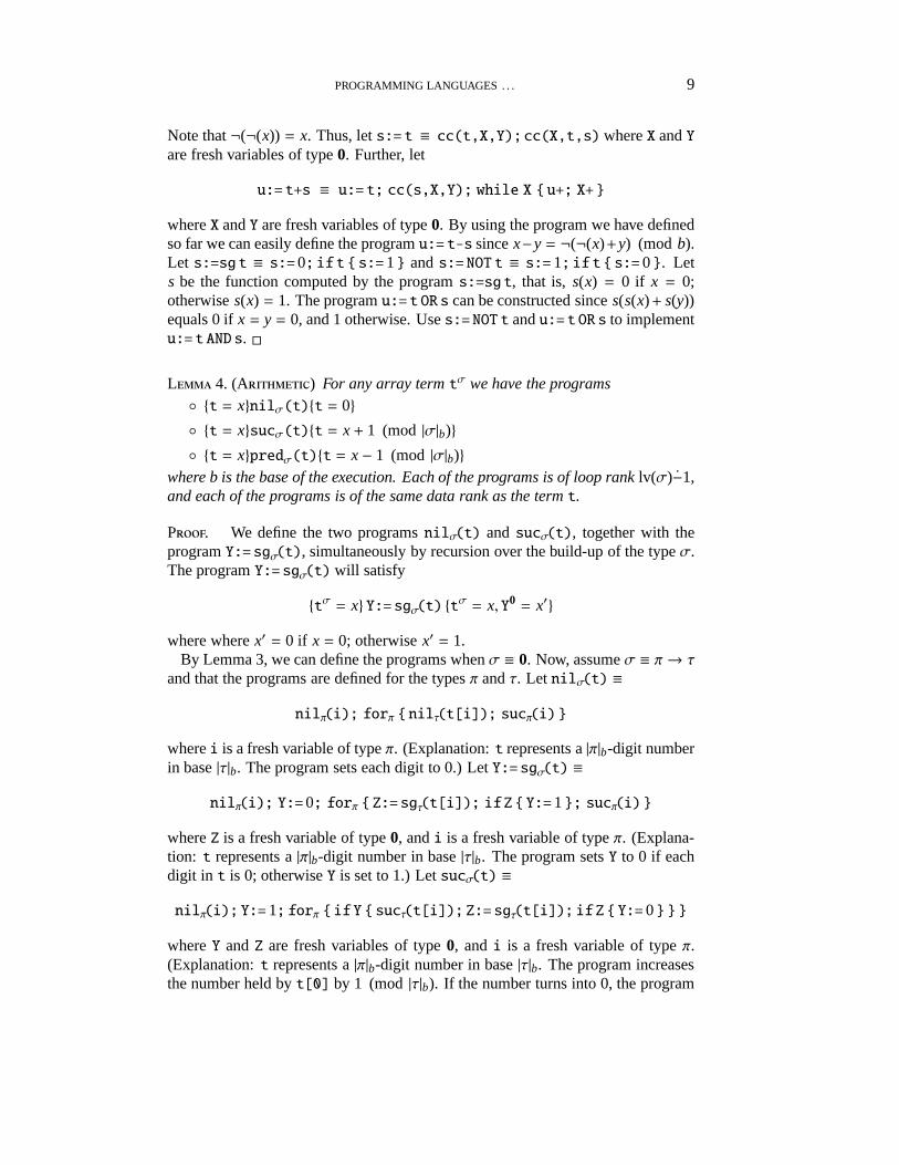
Note that¬(¬(x)) = x. Thus, lets:= t ≡ cc(t,X,Y);cc(X,t,s) whereX andYare fresh variables of type0. Further, let

u:=t+s ≡ u:= t; cc(s,X,Y); while X { u+; X+ }

whereX andY are fresh variables of type0. By using the program we have definedso far we can easily define the programu:= t-s sincex−y = ¬(¬(x)+y) (mod b).Let s:=sgt ≡ s:=0; if t { s:=1} ands:=NOT t ≡ s:= 1; if t{ s:= 0}. Lets be the function computed by the programs:=sgt, that is, s(x) = 0 if x = 0;otherwises(x) = 1. The programu:=t OR s can be constructed sinces(s(x)+ s(y))equals 0 ifx = y = 0, and 1 otherwise. Uses:=NOT t andu:=t OR s to implementu:=t ANDs. �

L 4. (A) For any array termtσ we have the programs◦ {t = x}nilσ(t){t = 0}

◦ {t = x}sucσ(t){t = x+ 1 (mod |σ|b)}

◦ {t = x}predσ(t){t = x− 1 (mod |σ|b)}where b is the base of the execution. Each of the programs is ofloop ranklv(σ)−1,and each of the programs is of the same data rank as the termt.

P. We define the two programsnilσ(t) andsucσ(t), together with theprogramY:=sgσ(t), simultaneously by recursion over the build-up of the typeσ.The programY:=sgσ(t) will satisfy

{tσ = x} Y:=sgσ(t) {tσ= x, Y0

= x′}

where wherex′ = 0 if x = 0; otherwisex′ = 1.By Lemma 3, we can define the programs whenσ ≡ 0. Now, assumeσ ≡ π→ τ

and that the programs are defined for the typesπ andτ. Let nilσ(t) ≡

nilπ(i); forπ { nilτ(t[i]); sucπ(i)}

wherei is a fresh variable of typeπ. (Explanation:t represents a|π|b-digit numberin base|τ|b. The program sets each digit to 0.) LetY:=sgσ(t) ≡

nilπ(i); Y:=0; forπ { Z:=sgτ(t[i]); ifZ { Y:=1}; sucπ(i)}

whereZ is a fresh variable of type0, andi is a fresh variable of typeπ. (Explana-tion: t represents a|π|b-digit number in base|τ|b. The program setsY to 0 if eachdigit in t is 0; otherwiseY is set to 1.) Letsucσ(t) ≡

nilπ(i); Y:= 1; forπ {if Y { sucτ(t[i]); Z:=sgτ(t[i]); if Z { Y:= 0} } }

whereY andZ are fresh variables of type0, andi is a fresh variable of typeπ.(Explanation:t represents a|π|b-digit number in base|τ|b. The program increasesthe number held byt[0] by 1 (mod|τ|b). If the number turns into 0, the program


increases the number held byt[1] by 1 (mod |τ|b). If the number turns into 0, thethe number held byt[2] is also modified, and so on.)

This completes the definition of the programsnilσ(t) andsucσ(t). Finally, letpredσ(t) be the programforσ {sucσ(t)}. We leave to the reader to check thatthe programs have the properties asserted by the lemma.�

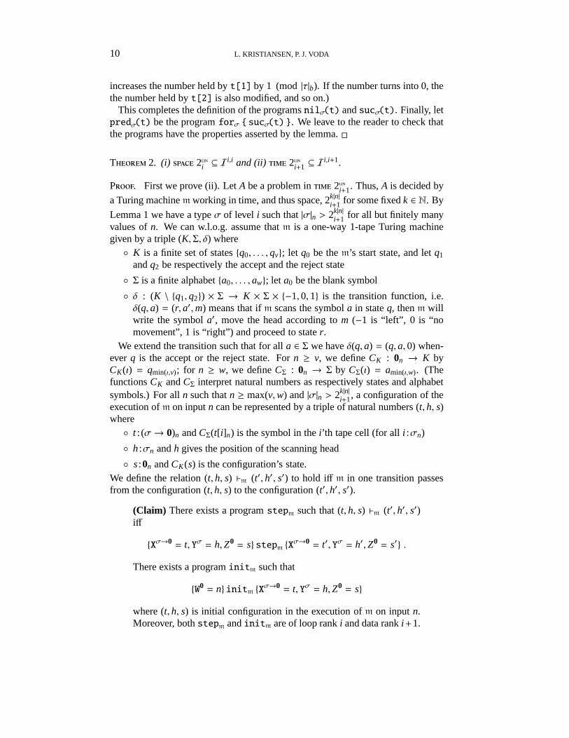
T 2. (i) 2i ⊆ Ii,i and (ii) 2i+1 ⊆ I

i,i+1.

P. First we prove (ii). LetA be a problem in 2i+1. Thus,A is decided by

a Turing machinem working in time, and thus space, 2k|n|i+1 for some fixedk ∈ N. By

Lemma 1 we have a typeσ of level i such that|σ|n > 2k|n|i+1 for all but finitely many

values ofn. We can w.l.o.g. assume thatm is a one-way 1-tape Turing machinegiven by a triple (K,Σ, δ) where◦ K is a finite set of states{q0, . . . , qv}; let q0 be them’s start state, and letq1

andq2 be respectively the accept and the reject state

◦ Σ is a finite alphabet{a0, . . . , aw}; let a0 be the blank symbol

◦ δ : (K \ {q1, q2}) × Σ → K × Σ × {−1, 0, 1} is the transition function, i.e.δ(q, a) = (r, a′,m) means that ifm scans the symbola in stateq, thenm willwrite the symbola′, move the head according tom (−1 is “left”, 0 is “nomovement”, 1 is “right”) and proceed to stater.

We extend the transition such that for alla ∈ Σ we haveδ(q, a) = (q, a, 0) when-everq is the accept or the reject state. Forn ≥ v, we defineCK : 0n → K byCK(ı) = qmin(ı,v); for n ≥ w, we defineCΣ : 0n → Σ by CΣ(ı) = amin(ı,w). (ThefunctionsCK andCΣ interpret natural numbers as respectively states and alphabetsymbols.) For alln such thatn ≥ max(v,w) and|σ|n > 2k|n|

i+1, a configuration of theexecution ofm on inputn can be represented by a triple of natural numbers (t, h, s)where◦ t : (σ→ 0)n andCΣ(t[i]n) is the symbol in thei’th tape cell (for alli :σn)

◦ h:σn andh gives the position of the scanning head

◦ s:0n andCK(s) is the configuration’s state.We define the relation (t, h, s) ⊢m (t′, h′, s′) to hold iff m in one transition passesfrom the configuration (t, h, s) to the configuration (t′, h′, s′).

(Claim) There exists a programstepm

such that (t, h, s) ⊢m (t′, h′, s′)iff

{Xσ→0= t, Yσ = h,Z0

= s} stepm{Xσ→0

= t′, Yσ = h′,Z0= s′} .

There exists a programinitm such that

{W0= n} initm {X

σ→0= t, Yσ = h,Z0

= s}

where (t, h, s) is initial configuration in the execution ofm on inputn.Moreover, bothstep

mandinitm are of loop ranki and data ranki+1.


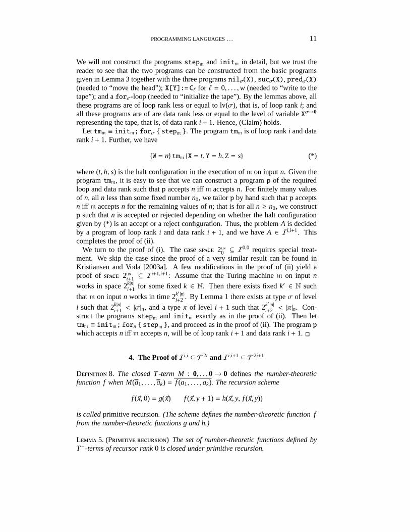
We will not construct the programsstepm

andinitm in detail, but we trust thereader to see that the two programs can be constructed from the basic programsgiven in Lemma 3 together with the three programsnilσ(X), sucσ(X), predσ(X)(needed to “move the head”);X[Y]:=Cℓ for ℓ = 0, . . . ,w (needed to “write to thetape”); and aforσ-loop (needed to “initialize the tape”). By the lemmas above, allthese programs are of loop rank less or equal to lv(σ), that is, of loop ranki; andall these programs are of are data rank less or equal to the level of variableXσ→0

representing the tape, that is, of data ranki + 1. Hence, (Claim) holds.Let tmm ≡ initm; forσ {stepm }. The programtmm is of loop ranki and data

rank i + 1. Further, we have

{W = n} tmm {X = t, Y = h, Z = s} (*)

where (t, h, s) is the halt configuration in the execution ofm on inputn. Given theprogramtmm, it is easy to see that we can construct a programp of the requiredloop and data rank such thatp acceptsn iff m acceptsn. For finitely many valuesof n, all n less than some fixed numbern0, we tailorp by hand such thatp acceptsn iff m acceptsn for the remaining values ofn; that is for alln ≥ n0, we constructp such thatn is accepted or rejected depending on whether the halt configurationgiven by (*) is an accept or a reject configuration. Thus, the problemA is decidedby a program of loop ranki and data ranki + 1, and we haveA ∈ Ii,i+1. Thiscompletes the proof of (ii).

We turn to the proof of (i). The case 20 ⊆ I0,0 requires special treat-

ment. We skip the case since the proof of a very similar resultcan be found inKristiansen and Voda [2003a]. A few modifications in the proof of (ii) yield aproof of 2i+1 ⊆ I

i+1,i+1: Assume that the Turing machinem on input n

works in space 2k|n|i+1 for some fixedk ∈ N. Then there exists fixedk′ ∈ N such

thatm on inputn works in time 2k′ |n|

i+2 . By Lemma 1 there exists at typeσ of level

i such that 2k|n|i+1 < |σ|n, and a typeπ of level i + 1 such that 2k′ |n|

i+2 < |π|n. Con-struct the programsstep

mandinitm exactly as in the proof of (ii). Then let

tmm ≡ initm; forπ { stepm }, and proceed as in the proof of (ii). The programpwhich acceptsn iff m acceptsn, will be of loop ranki + 1 and data ranki + 1. �

4. The Proof of Ii,i ⊆ F 2i and Ii,i+1 ⊆ F 2i+1

D 8. The closed T-term M: 0, . . . 0→ 0 definesthe number-theoreticfunction f when M(a1, . . . , ak) = f (a1, . . . , ak). The recursion scheme

f (~x, 0) = g(~x) f (~x, y+ 1) = h(~x, y, f (~x, y))

is calledprimitive recursion. (The scheme defines the number-theoretic function ffrom the number-theoretic functions g and h.)

L 5. (P ) The set of number-theoretic functions defined byT−-terms of recursor rank0 is closed under primitive recursion.


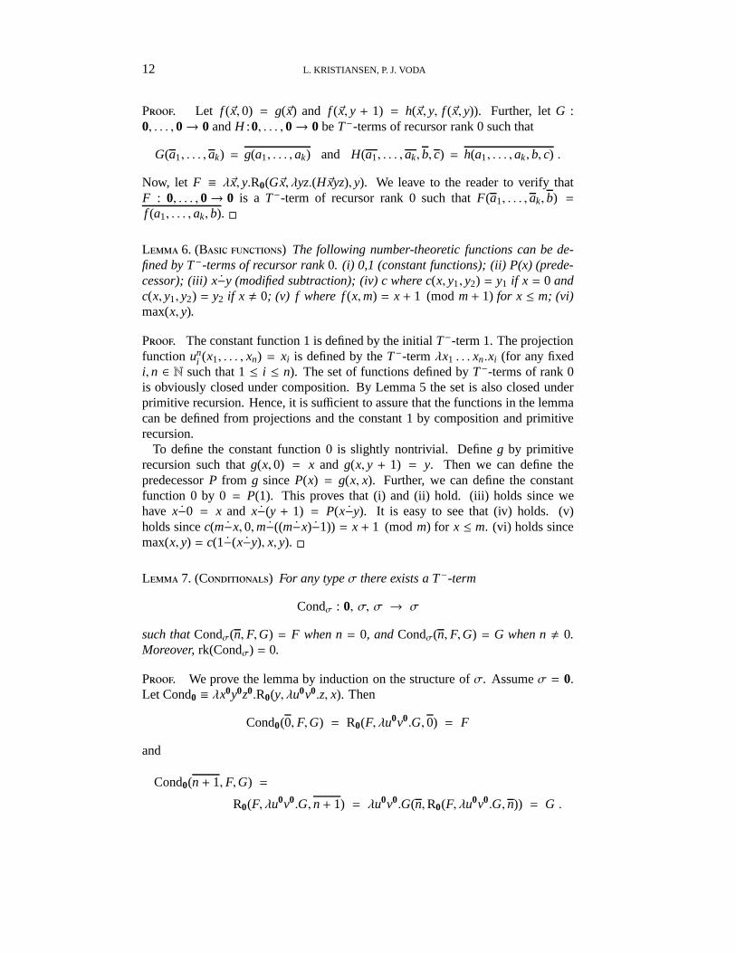
P. Let f (~x, 0) = g(~x) and f (~x, y + 1) = h(~x, y, f (~x, y)). Further, letG :0, . . . , 0→ 0 andH :0, . . . , 0→ 0 beT−-terms of recursor rank 0 such that

G(a1, . . . , ak) = g(a1, . . . , ak) and H(a1, . . . , ak, b, c) = h(a1, . . . , ak, b, c) .

Now, let F ≡ λ~x, y.R0(G~x, λyz.(H~xyz), y). We leave to the reader to verify thatF : 0, . . . , 0→ 0 is a T−-term of recursor rank 0 such thatF(a1, . . . , ak, b) =f (a1, . . . , ak, b). �

L 6. (B ) The following number-theoretic functions can be de-fined by T−-terms of recursor rank0. (i) 0,1 (constant functions); (ii) P(x) (prede-cessor); (iii) x−y (modified subtraction); (iv) c where c(x, y1, y2) = y1 if x = 0 andc(x, y1, y2) = y2 if x , 0; (v) f where f(x,m) = x+ 1 (modm+ 1) for x ≤ m; (vi)max(x, y).

P. The constant function 1 is defined by the initialT−-term 1. The projectionfunction un

i (x1, . . . , xn) = xi is defined by theT−-termλx1 . . . xn.xi (for any fixedi, n ∈ N such that 1≤ i ≤ n). The set of functions defined byT−-terms of rank 0is obviously closed under composition. By Lemma 5 the set is also closed underprimitive recursion. Hence, it is sufficient to assure that the functions in the lemmacan be defined from projections and the constant 1 by composition and primitiverecursion.

To define the constant function 0 is slightly nontrivial. Define g by primitiverecursion such thatg(x, 0) = x and g(x, y + 1) = y. Then we can define thepredecessorP from g sinceP(x) = g(x, x). Further, we can define the constantfunction 0 by 0= P(1). This proves that (i) and (ii) hold. (iii) holds since wehave x−0 = x and x−(y + 1) = P(x−y). It is easy to see that (iv) holds. (v)holds sincec(m−x, 0,m−((m−x)−1)) = x+ 1 (modm) for x ≤ m. (vi) holds sincemax(x, y) = c(1−(x−y), x, y). �

L 7. (C) For any typeσ there exists a T−-term

Condσ : 0, σ, σ → σ

such thatCondσ(n, F,G) = F when n= 0, andCondσ(n, F,G) = G when n, 0.Moreover,rk(Condσ) = 0.

P. We prove the lemma by induction on the structure ofσ. Assumeσ = 0.Let Cond0 ≡ λx0y0z0.R0(y, λu0v0.z, x). Then

Cond0(0, F,G) = R0(F, λu0v0.G, 0) = F

and

Cond0(n+ 1, F,G) =

R0(F, λu0v0.G, n+ 1) = λu0v0.G(n,R0(F, λu0v0.G, n)) = G .


Assumeσ = τ → ρ. Let Condσ ≡ λx0XσYσzτ.Condρ(x,Xz,Yz). Then, by theinduction hypothesis, we have Condσ(0, F,G) = λzτ.Condρ(0, Fz,Gz) = λzτ.Fz =F. The last equality holds since the calculus permitsη-reduction. By a similarargument, we have Condσ(n+ 1, F,G) = G. Assumeσ = τ × ρ. Let

Condσ ≡ λx0XσYσ.〈Condτ(x, fstX, fstY),Condρ(x, sndX, sndY)〉 .

Then, by the induction hypothesis, we have Condσ(n+ 1, F,G) =

〈Condτ(x, fstF, fstG),Condρ(x, sndF, sndG)〉 = 〈fstG, sndG〉 = G .

The last equality holds since the calculus permitsη-reductions. The proof thatCondσ(0, F,G) = F is similar. Obviously, we have rk(Condσ) = 0 for everyσ. �

D 9. For n ∈ N and terms M:σ→ σ, N :σ, let MnN denote the term Mrepeated n times on N, i.e. Mn+1N = M(MnN) and M0N = N.

L 8. (I) For all typesσ andτ there exists a T−-term

Itτσ : ( 0, τ→ τ, τ ) → τ

such thatItτσ(b, F,G) = F |σ|b+1G. Moreover, we haverk(Itτσ) = lv(σ) + lv(τ).

P. We prove the lemma by induction on the structure ofσ.Assumeσ = 0. Let Itτ0 ≡ λn

0Yτ→τXτ.Rτ(Y(X), λx0.Y, n). Obviously, we have

rk(Itτ0) = lv(0)+ lv(τ). We prove by induction onb that Itτσ(b, F,G) = Fb+1(G). Wehave Itτσ(0, F,G) = Rτ(F(G), λx.F, 0) = F(G). By induction hypothesis we have

Itτσ(b+ 1, F,G) = Rτ(F(G), λx.F, b+ 1) = (λx.F)bRτ(F(G), λx.F, b) =

(λx.F)bItτσ(b, F,G) = FFb+1G = Fb+2G .

Thus, the lemma holds whenσ = 0 since|0|b+1 = b+ 1.Assumeσ = σ1 × σ2. Let Itτσ ≡ λx

0Yτ→τXτ.Itτσ1(x, Itτσ2

(x,Y),X). Thus,

rk(Itτσ) = max(rk(Itτσ1), rk(Itτσ2

)) def. of rk

= max(lv(σ1) + lv(τ), lv(σ2) + lv(τ)) ind. hyp.

= max(lv(σ1), lv(σ2)) + lv(τ)

= lv(σ1 × σ2) + lv(τ) def. of lv

= lv(σ) + lv(τ) . σ = σ1 × σ2

This proves that rk(Itτσ) has the right recursor rank. Further, we have

Itτσ(b, F,G) = Itτσ1(b, Itτσ2

(b, F),G) def. of Itτσ= Itτσ2

(b, F)|σ1|b+1(G) ind. hyp. onσ1

= F |σ1|b+1×|σ2|b+1(G) ind. hyp. onσ2

= F |σ|b+1(G) . def. of |σ|b+1


Assumeσ = σ1→ σ2. Let Itτσ ≡ λx0Yτ→τXτ.(Itτ→τσ1

(x, Itτσ2(x),Y)X). We have

rk(Itτσ) = max(rk(Itτ→τσ1), rk(Itτσ2

)) def. of rk

= max(lv(σ1) + lv(τ→ τ), lv(σ2) + lv(τ)) ind. hyp.

= max(lv(σ1) + lv(τ) + 1, lv(σ2) + lv(τ)) def. of lv

= max(lv(σ1) + 1, lv(σ2)) + lv(τ)

= lv(σ) + lv(τ) . def. of lv

So, the iterator has the right recursor rank. We will now prove that we indeedhave Itτσ(b, F,G) = F |σ|b+1G. Let A ≡ (Itτσ2

b). We prove by induction onk that

(AkF)G = F |σ2|kb+1G (*). We have (A0F) = F, and hence (A0F)G = F |σ2|

0b+1G.

Further, we have

(Ak+1F)G = (A(AkF))G = Itτσ2(b,AkF,G) = (AkF)|σ2|b+1G = F |σ2|

k+1b+1G.

The two last equalities hold by the induction hypothesis onσ2 andk respectively.This proves (*), and hence

Itτσ(b, F,G) = Itτ→τσ1(b, (Itτσ2

b), F)G def. of Itτσ= (Itτσ2

b)|σ1|b+1F)G ind. hyp. onσ1

= F |σ2||σ1|b+1b+1 G (*)

= F |σ|b+1G . def. of |σ|b+1

completes the proof of the theorem.�

We will interpret terms as natural numbers. Letb > 1, and letM be a closedT-term of typeσ. The interpretationvalb(M) defined below evaluatesM to a naturalnumber of typeσb, that is, to a natural number strictly less than|σ|b.

D 10. LetV be a valuation, that is a set of pairs x/v where x is a variableand v∈ N. For any T-term M we define thevalue ofM at the basebunder valuationV, writtenvalVb (M).

◦ Let valVb (0) = 0; valVb (1) = 1; valVb (x) = v if x is a variable and x/v ∈ V.

◦ Let valVb (sM) = valVb (M) + 1 (modb).

◦ Let valVb ((MN)) = valVb (M)[valVb (N)]b.

◦ Let valVb (λxσMτ) =∑

i<|σ|b valV′

b (M) × |τ|ib whereV′ = V ∪ {x/i}.

◦ Let valVb (fstMσ×τ) = valVb (M) div |τ|b (integer division).

◦ Let valVb (sndMσ×τ) = valVb (M) mod|τ|b.

◦ Let valVb (〈Mσ,Nτ〉) = valVb (M) × |τ|b + valVb (N).

◦ Recall that Rσ has typeσ, 0→ σ→ σ, 0→ σ. Letπ = 0→ σ→ σ, 0→ σ;let ρ = 0→ σ→ σ; let

valVb (Rσ) =∑

u<|σ|b

|π|ub × (∑

w<|ρ|b

|0→ σ|wb × (∑

n<|0|b

|σ|nb × Υn))

whereΥ0= u andΥn+1

= w[n]b[Υn]b.


For any closed term M letvalb(M) = val∅b(M).

L 9. (V) The functionval has the following properties.(i) Let M and N be T−-terms of any type such that M⊲ N. Fix some b> 1. LetV be a valuation of the free variables in M such that ifV assigns the valuev to the variable x:σ, then v< |σ|b. Then we havevalVb (M) = valVb (N).

(ii) Let M and N be closed T-terms of any type such that M⊲ N. We havevalb(M) = valb(N) for all sufficiently large b.

(iii) Let M :0→ 0 be a closed T−-term. We have Mn = m iff valb(Mn) = m for allb > max(n, 1), and in particular, we havevalmax(n,1)+1(Mn) = m iff Mn = m.

P. The proof of clause (i) and (ii) are straightforward, but very tedious. Weskip the details. Clause (iii) follows from clause (i) and (ii) since the reductionprocess in the calculusT normalizes andvalb(n) = n for anyb > n. �

Note that clause (ii) of Lemma 9 does not hold for smallb, e.g.fst〈10, 2〉 ⊲ 10,but val2(fst〈10, 2〉) = (10 × 2 + 2) div 2 = 11 andval2(10) = 0. The equalityvalb(fst〈10, 2〉) = valb(10) holds for allb > 10.

L 10. (A) For any typeσ there exists T−-terms

0σ :0 , Sucσ :0, σ→ σ , Leσ :0, σ, σ→ 0 and Eqσ :0, σ, σ→ 0

such that(i) valb+1(0σ) = 0 andvalb+1(Sucσ(b, F)) = valb+1(F) + 1 (mod |σ|b+1)

(ii) Leσ(b, F,G) = 0 iff valb+1(F) ≤ valb+1(G)

(iii) Eqσ(b, F,G) = 0 iff valb+1(F) = valb+1(G)for any closed T-terms F and G. Moreover,Sucσ, Leσ and Eqσ have recursorranks≤ 2lv(σ)−2 (and0σ has recursor rank 0).

P. We prove (i), (ii) and (iii) by induction on structure ofσ. It follows fromLemma 6 that there are suchT−-terms whenσ = 0.

Assume thatσ = π→ τ. Let 0σ ≡ λxπ.0τ. Obviously, rk(0σ) = 0. LetF ≡

λb0Xπ→τYπ→τz0×π.

Cond0×π(Eqτ(b,X(sndz),Y(sndz)), 〈fstz,Sucπ(b, sndz)〉,

Cond0×π(Leτ(b,X(sndz),Y(sndz)), 〈00,Sucπ(b, sndz)〉,

〈1,Sucπ(b, sndz)〉)) .

Let M, N and j be closed terms. By the induction hypothesis, we have

F(b,M,N, 〈i, j〉) =

〈i,Sucπ( j)〉 if valb+1(M)[valb+1( j)]b+1 = valb+1(N)[valb+1( j)]b+1

〈0,Sucπ( j)〉 if valb+1(M)[valb+1( j)]b+1 < valb+1(N)[valb+1( j)]b+1

〈1,Sucπ( j)〉 otherwise.


Hence, (ii) and (iii) hold when Leσ ≡ λbXY.fstIt0×ππ (b, F(b,X,Y), 〈00, 0π〉) and

Eqσ ≡ λbXY.Cond0(Leσ(b,X,Y),Cond0(Leσ(b,Y,X), 00, 1), 1). We will now ar-gue that Leσ and Eqσ have the required recursor rank. First, we note that rk(F) ≤max(2lv(π)−2, 2lv(τ)−2) (*). (Lemma 7 states that rk(Cond0×π) = 0, and then (*)follows from the induction hypothesis.) Further,

rk(Eqσ) = rk(Leσ) def. of rk, def. of Eqσ= max(rk(F), rk(It0×π

π )) def. of rk, def. of Leσ

≤ max(rk(F), lv(π) + lv(0 × π)) Lemma 8

≤ max(2lv(π)−2, 2lv(τ)−2, 2lv(π)) (*)

= max(2lv(τ)−2, 2lv(π))

= max(2(lv(τ)−1), 2lv(π))

= 2 max(lv(π), lv(τ)−1)

= 2(max(lv(π) + 1, lv(τ))−1)

= 2(lv(σ)−1) def. of lv,σ = π→ τ

= 2lv(σ)−2 .

Thus, Eqσ and Leσ have the required rank. Next we define Sucσ. Let a : σb anda′ :σb be such thata′ = a+ 1 (mod |σ|b) anda = v0|τ|

0b+ v1|τ|

1b+ · · ·+ vk|τ|

kb where

k = |π|b− 1 andv0, . . . , vk are digits of typeτb. Then there existsi ∈ {0, . . . , k} suchthat

a′ = v′0|τ|0b + · · · + v′i |τ|

ib + vi+1|τ|

i+1b + · · · + vk|τ|

kb

wherev′j = v j +1 (mod |τ|b) for j = 0, . . . , i. We call such ani for thecarry border

for the numbera:σb. Let Cσ ≡ λbX.snd It0×ππ (b,G(b,X), 〈0, 0π〉) where

G ≡ λb0Xπ→τz0×π.Cond0(fst z,Cond0×π(Eqτ(b,Sucτ(X(sndz)), 0τ),

〈0,Sucπ(sndz)〉, 〈1,Sucπ(sndz)〉), 〈1,Sucπ(sndz)〉)

Then, valb+1(C(b,M)) equals the carry border forvalb+1(M) when M : σ is aclosed term. Let Sucσ ≡ λb0Xσiπ.Condτ(Leπ(b, i,Cσ(b,X)),Sucτ(X(i)),X(i)) and(i) holds. By an argument similar to the one showing that the ranks of Eqσ andLeσ are bounded by 2lv(σ)−2, we can show that the rank of Cσ also is bounded by2lv(σ)−2. The rank of Sucσ equals the rank of Cσ.

Assume thatσ = π × τ. Let 0σ ≡ 〈0π, 0τ〉. Define Sucσ such that

Sucσ(b, 〈F,G〉) =

〈Sucπ(F),Sucτ(G)〉 if Eqτ(b,Sucτ(G)) = 0τ〈F,Sucτ(G)〉 otherwise.

Define Leσ such that Leσ(b, 〈F,G〉, 〈F′,G′〉) = 0 iff

(Leπ(b, F, F′) = 0 ∧ Eqπ(b, F, F

′) > 0) ∨

(Leπ(b,G,G′) = 0 ∧ Eqπ(b, F, F

′) = 0)


and Eqσ such that Eqσ(b, F,G) = 0 iff Leσ(b, F,G) = 0 ∧ Leσ(b,G, F) = 0. Itis easy to constructT−-terms Sucσ, Leσ and Eqσ with the required properties andrecursor ranks. We skip the details.�

L 11. (M) For any types~σ = σ1, . . . , σk andτ there exists a T−-termMd~σ→τ :0, ~σ→ τ, ~σ, τ→ ~σ→ τ such that

Md~σ→τ(b, F, ~G,V)( ~H) =

{

V if valb+1(Gi) = valb+1(Hi) for i = 1, . . . , kF( ~H) otherwise.

for any closed T-terms Gi : σi and Hi : σi. Moreover, we haverk(Md~σ→τ) ≤2 max(lv(σ1), . . . , lv(σk))−2 (*).

P. We prove the lemma by induction on the length of~σ. Assume, the lengthof ~σ equals 1, then~σ = ρ for some typeρ. Let

Mdρ→τ ≡ λb0Fρ→τXρVτYρ.Condτ(Eqρ(b,X,Y),V, F(Y)) .

Assume, the length of~σ is strictly greater than 1, then~σ = ρ, ~π. Assume, by theinduction hypothesis, that Mdρ→τ and Md~π→τ are defined. Let

Mdρ,~π→τ ≡ λb0Fρ,~π→τXρ0Xπ1

1 . . .Xπkk Vτ.

Mdρ→τ(b, F,X0,Md~π→τ(b, F(X0),X1, . . . ,Xk,V)) .

It is easy to see that rk(Md~σ→τ) = max(rk(Eqσ1), . . . , rk(Eqσk

), rk(Condτ)). Thus,(*) holds by Lemma 7 and Lemma 10.�

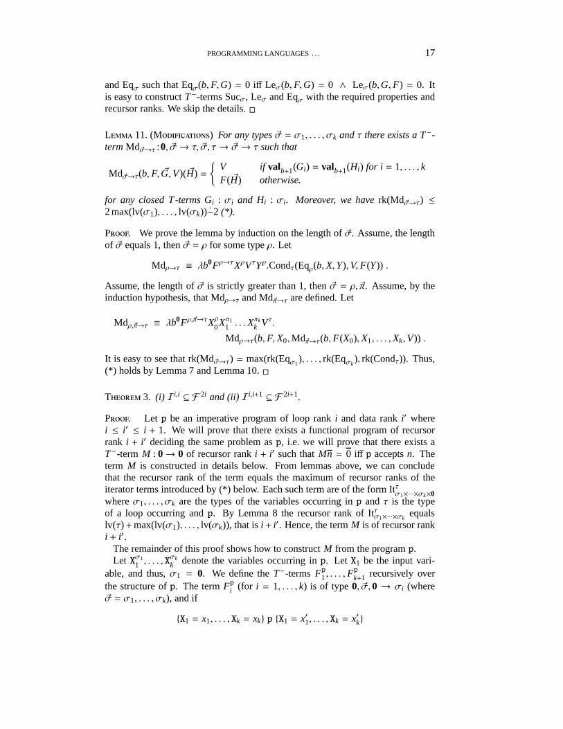
T 3. (i) Ii,i ⊆ F 2i and (ii) Ii,i+1 ⊆ F 2i+1.

P. Let p be an imperative program of loop ranki and data ranki′ wherei ≤ i′ ≤ i + 1. We will prove that there exists a functional program of recursorrank i + i′ deciding the same problem asp, i.e. we will prove that there exists aT−-term M : 0→ 0 of recursor ranki + i′ such thatMn = 0 iff p acceptsn. Theterm M is constructed in details below. From lemmas above, we can concludethat the recursor rank of the term equals the maximum of recursor ranks of theiterator terms introduced by (*) below. Each such term are ofthe form Itτ

σ1×···×σk×0whereσ1, . . . , σk are the types of the variables occurring inp andτ is the typeof a loop occurring andp. By Lemma 8 the recursor rank of Itτσ1×···×σk

equalslv(τ)+max(lv(σ1), . . . , lv(σk)), that isi + i′. Hence, the termM is of recursor ranki + i′.

The remainder of this proof shows how to constructM from the programp.Let Xσ1

1 , . . . , Xσkk denote the variables occurring inp. Let X1 be the input vari-

able, and thus,σ1 = 0. We define theT−-termsFp1, . . . , Fp

k+1 recursively overthe structure ofp. The termFpi (for i = 1, . . . , k) is of type0, ~σ, 0 → σi (where~σ = σ1, . . . , σk), and if

{X1 = x1, . . . , Xk = xk} p {X1 = x′1, . . . , Xk = x′k}


whenp is executed in a sufficiently large baseb+ 1, then

valb+1(Gℓ) = xℓ for ℓ = 1, . . . , k ⇒ valb+1(Fpj (b,G1, . . . ,Gk, y)) = x′j

for any closedT-termsGσ11 , . . . ,G

σkk . Further, we will construct the terms such

that p acceptsn iff Fpk+1(max(n, 1), n,G2, . . . ,Gk, 1)) = 0 for any closed termsGσ2

2 , . . . ,Gσkk .

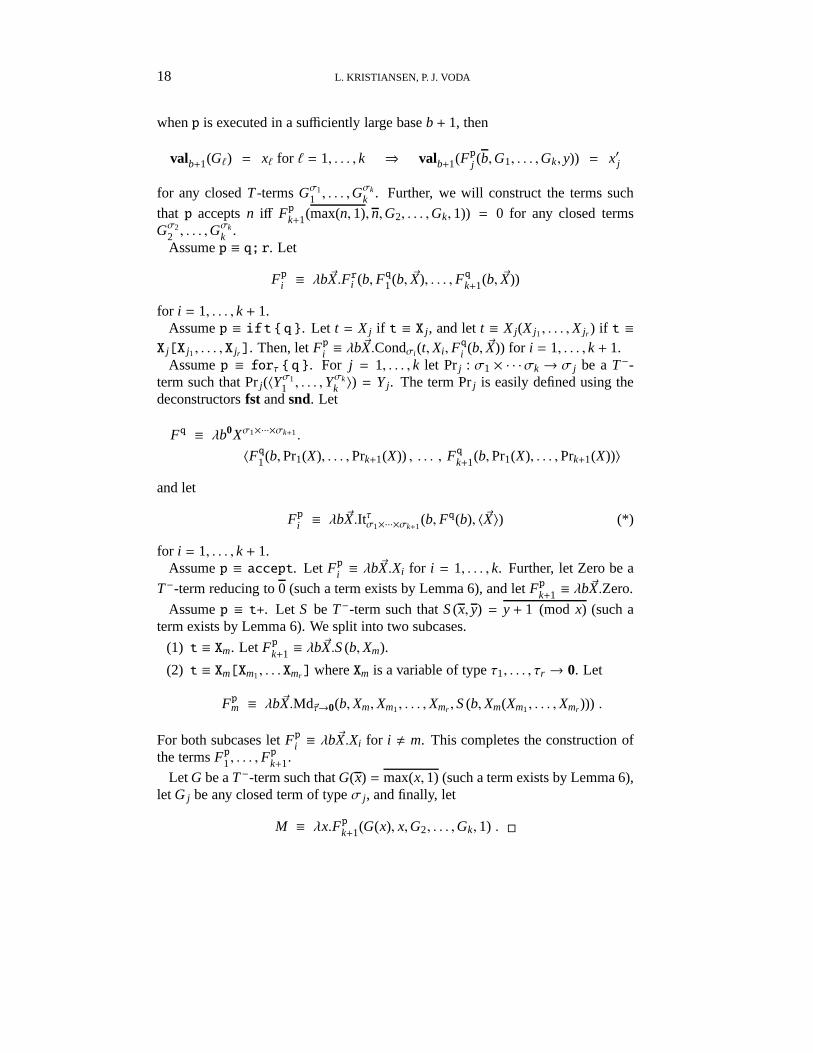
Assumep ≡ q; r. Let

Fpi ≡ λb~X.Fri (b, Fq1(b, ~X), . . . , Fqk+1(b, ~X))

for i = 1, . . . , k+ 1.Assumep ≡ ift { q }. Let t = X j if t ≡ X j , and lett ≡ X j(X j1, . . . ,X jr ) if t ≡X j[X j1, . . . , X jr]. Then, letFpi ≡ λb

~X.Condσi (t,Xi , Fq

i (b, ~X)) for i = 1, . . . , k+ 1.Assumep ≡ forτ { q }. For j = 1, . . . , k let Prj : σ1 × · · ·σk → σ j be aT−-

term such that Prj(〈Yσ11 , . . . ,Y

σkk 〉) = Yj. The term Prj is easily defined using the

deconstructorsfst andsnd. Let

Fq ≡ λb0Xσ1×···×σk+1.

〈Fq1(b,Pr1(X), . . . ,Prk+1(X)) , . . . , Fqk+1(b,Pr1(X), . . . ,Prk+1(X))〉

and let

Fpi ≡ λb~X.Itτσ1×···×σk+1

(b, Fq(b), 〈~X〉) (*)

for i = 1, . . . , k+ 1.Assumep ≡ accept. Let Fpi ≡ λb

~X.Xi for i = 1, . . . , k. Further, let Zero be a

T−-term reducing to0 (such a term exists by Lemma 6), and letFpk+1 ≡ λb~X.Zero.

Assumep ≡ t+. Let S be T−-term such thatS(x, y) = y+ 1 (mod x) (such aterm exists by Lemma 6). We split into two subcases.

(1) t ≡ Xm. Let Fpk+1 ≡ λb~X.S(b,Xm).

(2) t ≡ Xm[Xm1, . . .Xmr] whereXm is a variable of typeτ1, . . . , τr → 0. Let

Fpm ≡ λb~X.Md~τ→0(b,Xm,Xm1, . . . ,Xmr ,S(b,Xm(Xm1, . . . ,Xmr ))) .

For both subcases letFpi ≡ λb~X.Xi for i , m. This completes the construction of

the termsFp1, . . . , Fp

k+1.

Let G be aT−-term such thatG(x) = max(x, 1) (such a term exists by Lemma 6),let G j be any closed term of typeσ j, and finally, let

M ≡ λx.Fpk+1(G(x), x,G2, . . . ,Gk, 1) . �


5. The proof of F 2i ⊆ 2i and F 2i+1 ⊆ 2i+1

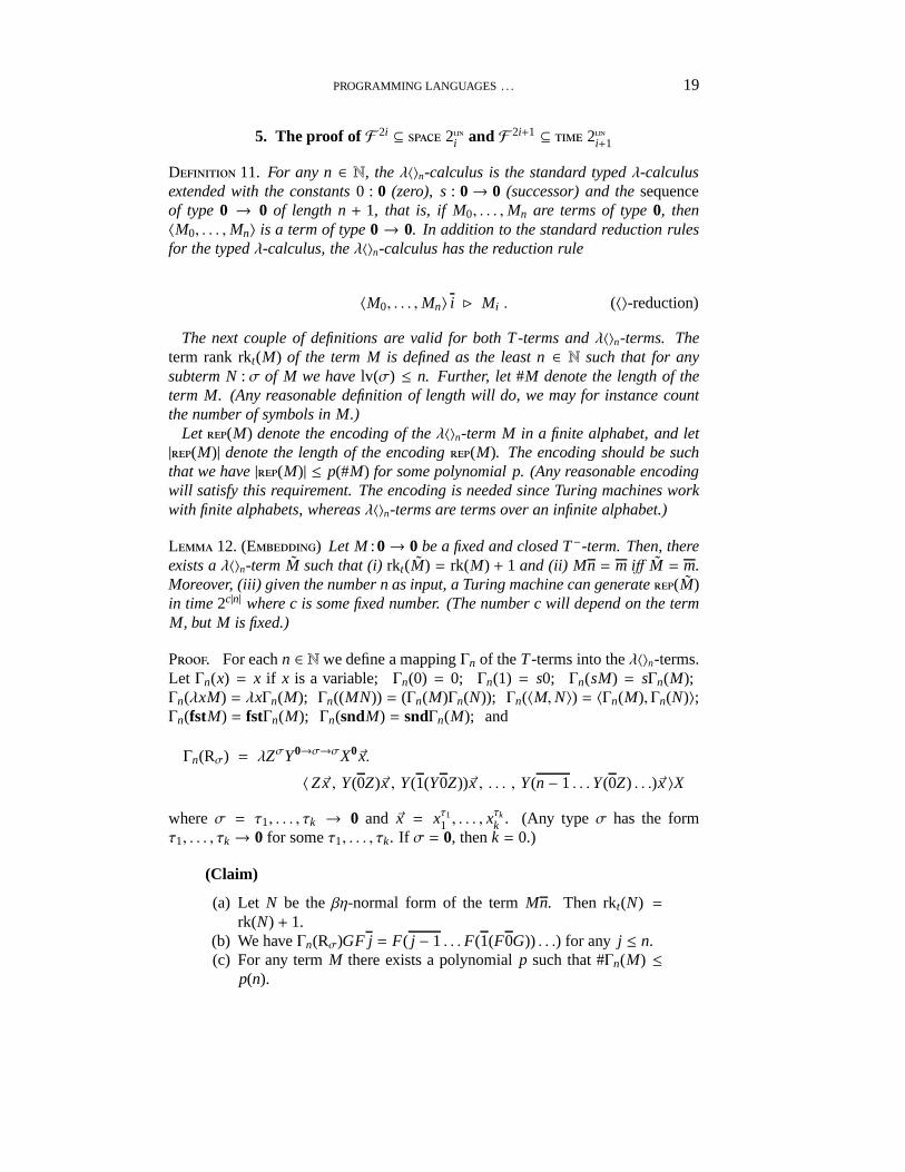
D 11. For any n ∈ N, theλ〈〉n-calculus is the standard typedλ-calculusextended with the constants0 : 0 (zero), s: 0→ 0 (successor) and thesequenceof type0 → 0 of length n+ 1, that is, if M0, . . . ,Mn are terms of type0, then〈M0, . . . ,Mn〉 is a term of type0 → 0. In addition to the standard reduction rulesfor the typedλ-calculus, theλ〈〉n-calculus has the reduction rule

〈M0, . . . ,Mn〉 i ⊲ Mi . (〈〉-reduction)

The next couple of definitions are valid for both T-terms andλ〈〉n-terms. Theterm rank rkt(M) of the term M is defined as the least n∈ N such that for anysubterm N: σ of M we havelv(σ) ≤ n. Further, let#M denote the length of theterm M. (Any reasonable definition of length will do, we may for instance countthe number of symbols in M.)

Let (M) denote the encoding of theλ〈〉n-term M in a finite alphabet, and let|(M)| denote the length of the encoding(M). The encoding should be suchthat we have|(M)| ≤ p(#M) for some polynomial p. (Any reasonable encodingwill satisfy this requirement. The encoding is needed sinceTuring machines workwith finite alphabets, whereasλ〈〉n-terms are terms over an infinite alphabet.)

L 12. (E) Let M:0→ 0 be a fixed and closed T−-term. Then, thereexists aλ〈〉n-term M such that (i)rkt(M) = rk(M) + 1 and (ii) Mn = m iff M = m.Moreover, (iii) given the number n as input, a Turing machinecan generate(M)in time2c|n| where c is some fixed number. (The number c will depend on the termM, but M is fixed.)

P. For eachn ∈ N we define a mappingΓn of theT-terms into theλ〈〉n-terms.Let Γn(x) = x if x is a variable; Γn(0) = 0; Γn(1) = s0; Γn(sM) = sΓn(M);Γn(λxM) = λxΓn(M); Γn((MN)) = (Γn(M)Γn(N)); Γn(〈M,N〉) = 〈Γn(M), Γn(N)〉;Γn(fstM) = fstΓn(M); Γn(sndM) = sndΓn(M); and

Γn(Rσ) = λZσY0→σ→σX0~x.

〈Z~x , Y(0Z)~x , Y(1(Y0Z))~x , . . . , Y(n− 1 . . .Y(0Z) . . .)~x 〉X

whereσ = τ1, . . . , τk → 0 and ~x = xτ11 , . . . , xτkk . (Any type σ has the form

τ1, . . . , τk → 0 for someτ1, . . . , τk. If σ = 0, thenk = 0.)

(Claim)

(a) Let N be theβη-normal form of the termMn. Then rkt(N) =rk(N) + 1.

(b) We haveΓn(Rσ)GF j = F( j − 1 . . . F(1(F0G)) . . .) for any j ≤ n.(c) For any termM there exists a polynomialp such that #Γn(M) ≤

p(n).


We prove clause (a) of (Claim). Obviously, it cannot be the case that rkt(N) <rk(N)+ 1. Suppose that rkt(N) > rk(N)+ 1. Then there exists a subtermN′ :ρ→ τof N such that rkt(N′) = rkt(N) = lv(ρ → τ) > rk(N) + 1. First we note thatN′

cannot be a variable. (BecauseN is a closed term, and ifN′ were a variable, wewould have rkt(N) > lv(ρ → τ).) Thus,N′ has the formλxρ.Pτ, and sinceN hastype0 there will be a subterm ofN on the formλxρ.PτQρ. This contradicts thatNis in theβη-normal form. This proves (a). Further, we have

Γn(Rσ)GF j = λ~x.(F( j − 1 . . .F(0G) . . .)~x) = F( j − 1 . . .F(1F(0G)) . . .) .

The first equality holds by threeβ-reduction and one〈〉-reduction; the secondequality holds byk η-reductions. Hence, we see that clause (b) of (Claim) holds.Iteasy to see that clause (c) of (Claim) holds by inspecting thedefinition ofΓn.

Let N be theβη-normal form of the termMn, and letM be the termΓn(N). Itfollows from respectively (a) and (b) that respectively (i)and (ii) hold. Further,it is easy to see that #N is bounded by a polynomial inn, and then by (c), #M isbounded by a polynomial inn. Our encoding scheme for terms guarantees that also|(M)| will be bounded by a polynomial inn. It is easy to see that there exists apolynomial p such that(M) can be generated by a Turing machine in no morethanp(|(M)|) steps. This entails that there exists a fixedc ∈ N such that(M)can be generated in time 2c|n|. Hence, (iii) holds.�

D 12. We extend the definition ofvalb given at page 14 by

valVb (〈M0, . . . ,Mn〉) =∑

i<n+1

valVb (Mi) × |0|ib .

(Thus,valn+1(M) is defined for any closedλ〈〉n-term M.)

L 13. Let M:0 be a closedλ〈〉n-term of term rank k+ 2.(i) There exist a polynomial p and a constant c∈ N such thatvaln+1(M) can be

computed by a Turing machine in space p(|(M)|) × 2c|n|k .

(ii) There exist a polynomial p and a constant c∈ N such thatvaln+1(M) can be

computed by a Turing machine in time p(|(M)|) × 2c|n|k+1.

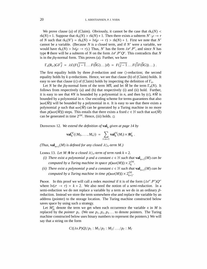
P. In this proof we will call a redexmaximalif it is of the form (λxσ.Pτ)Qσ

where lv(σ → τ) = k + 2. We also need the notion of asemi-reduction. In asemi-reduction we do not replace a variable by a term as we do in an ordinaryβ-reduction. Instead we store the term somewhere else and replace the variable by anaddress (pointer) to the storage location. The Turing machine constructed belowsaves space by using such a strategy.

Let Mxpi

denote the term we get when each occurrence the variablex in M isreplaced by thepointer pi . (We usep1, p2, p3 . . . to denote pointers. The Turingmachine constructed below uses binary numbers to representthe pointers.) We willsay that a string on the form

C{(λx.P)Q}/p1 : M1/p2 : M2/ . . . /pℓ : Mℓ


(whereC{(λx.P)Q} is a representation of aλ〈〉n-term possibly containing pointerswith maximal redex (λx.P)Q, and whereM1, . . . ,Mℓ,P,Q are representations ofλ〈〉n-terms possibly containing pointers)semi-reducesto the string

C{Pxpℓ+1}/p1 : M1/p2 : M2/ . . . /pℓ : Mℓ/pℓ+1 : Q .

Let M :0 be the closedλ〈〉n-term of term rankk+ 2 given in the lemma. We willconstruct a Turing machine computingvaln+1(M). Let w0 be(M). The Turingmachine starts withw0 on its work tape, picks a maximal redex inw0 and semi-reducesw0 to w1. It will pick the leftmost maximal redex (λxPR) such that thereare no maximal redexes insideR. Thereafter it semi-reducesw1 to w2 following thesame procedure, thenw2 to w3, and so on. Sooner or later, say after steps, the pro-cess will terminate since there will be no maximal redexes left. The stringw hasthe formP/p1 : M1/p2 : M2/ . . . /p : M and represents aλ〈〉n-term of term rankk + 1. (Note that no semi-reductions will take place inside the termsM1, . . . ,M since these terms do not contain maximal redexes.) The Turing machine can movefreely back and forth in the represented term by following the pointers and pushingthe return addresses on a stack. It should be obvious that we could construct theTuring machine such that

the number of steps the Turing machine needs to generatew fromthe input(M) is bounded byp(|(M)|) for some polynomialp. (*)

Let Q be the term of term rankk + 1 represented byw. We havevaln+1(Q) =valn+1(M). After generatingw, the Turing machine will computevaln+1(Q) usingregisters. A register is nothing but a marked area on one of the tapes dedicated tostore a natural number. The functionvalVn+1 is defined recursively over the structureof λ〈〉n-terms. The Turing machine will compute the valuevalVn+1(S) of a composedtermS by computing the values of its subterms, store the results away in registers,and then retrieve the results when they are needed in the computation ofvalVn+1(S).E.g. to compute the valuevalVn+1((λx.S)R), the Turing machine will first computea = valVn+1(λxS), storea in a register, thereafter computeb = valVn+1(R), storeb ina register, and finally compute the valuevalVn+1((λx.S)R) by computing the numbera[b]n+1. The Turing machine will only depart from this natural recursive procedurewhen it encounters subterms of levelk+1. There will be some such subterms sinceQ is of term rankk + 1. For the sake of the argument assume that such a subtermhas formλxRwhere rkt(R) = k. In such a case the Turing machine will computethe valuevalVn+1((λx.R)S) by first computinga = valVn+1(S) and then compute thevaluevalV

′

n+1(R) whereV′ = V ∪ {x/a}. It should be obvious that it is possible todesign the Turing machine such that it never will store numbers of typeσ wherelv(σ) = k+ 1.

We will now argue that the Turing machine sketched above works within thespace and time constrains stated in the lemma. First the Turing machine generatesw, and by (*), it needs no more thanp(|(M)|) tape cells to do so. Then the Tur-ing machine computesvaln+1(M) by using registers. The greatest number stored ina register during the computation is bounded by|ξ|n+1 whereξ is of levelk. Lemma


2 says there exists a constantc1 ∈ N such that|ξ|n+1 ≤ 2c1|n|k+1 . The Turing machine

represents the numbers in the registers in binary, and hencethe number of tapecells required for one register is bounded by 2c2|n|

k for some constantc2 ∈ N. Thetotal number of registers required will be bounded by the length of w, and thus,the total number of tape cells required will be bounded byp(|(M)|) × 2c|n|

k forsome polynomialp and somec ∈ N. This proves (i). The proof of (ii) is similar.�

L 14. (R R) Let M : 0 be a closedλ〈〉n-term of term rank k+ 2.(i) There exists aλ〈〉n-term N of term rank k+ 1 such that M= N and#N ≤ 2c#M

for some fixed c∈ N. Moreover, (ii) given(M) as input, a Turing machine cangenerate(N) in time2c|(M)| for some fixed c∈ N.

P. The proof of (i) is similar to the standard proofs found in the literaturefor eliminating “cuts” in the typedλ-calculus. See Schwichtenberg [1982] andBeckmann [2001]. Since each sequence is of type0 → 0, there will be no〈〉-reductions involved in the rank reduction process from rankk+ 2 to rankk+ 1.

We argue that also (ii) holds. The rank reduction process might introduce newvariables (in order to avoid thatβ-reductions result in name conflicts). Still, thenumber of variables inN will be bounded by 2c#M , and thus, using a reasonableencoding scheme, we have|(N)| ≤ 2c′ |(M)| for somec′ ∈ N. The number ofsteps required to generate(N) is bounded byp(|(N)|) for some polynomialp,and thus also bounded by 2c|(M)| for somec ∈ N. �

T 4. (i) F 2i ⊆ 2i and (ii) F 2i+1 ⊆ 2i+1.

P. We prove (i). The proof splits into the casesi = 0 andi > 0.Case i> 0. Then i = k + 1 and 2i = 2k + 2 for somek ∈ N. Let M : 0→ 0 be

a closedT−-term of rank 2k + 2. We will prove that there exists a Turing machinewhich on inputn works in space 2c|n|k+1 for some constantc ∈ N, and computes thenumberm such thatMn = m.

First, the Turing machine generates the representation(M) of theλ〈〉n-term Mgiven in Lemma 12. The termM is of term rank 2k + 3, and(M) is generatedin time 2c0|n| for some fixedc0 ∈ N. Thereafter, the Turing machine generatesthe representation(P) of a λ〈〉n-term P of term rankk + 3 such thatP = M.By Lemma 14, we havec1 ∈ N such that(P) can be generated from(M)

in time 2c1|(M)|k . Thus, there existsc2 ∈ N such that(P) is generated from

n in time (and hence also in space) 2c2|n|k+1 . Finally, the Turing machine computes

the valuevaln+1(P). By Lemma 13 it is possible for a Turing machine to complete

this task in spacep((P)) × 2c3|n|k+1 wherep is a polynomial andc3 ∈ N. Note that

p((P)) × 2c3|n|k+1 ≤ p(2c2|n|

k+1 ) × 2c3|n|k+1 ≤ 2c|n|

k+1 holds for some fixedc ∈ N.Case i= 0. Let M : 0→ 0 be a closedT−-term of rank 0. Letx : 0 be a variable

not occurring inM, and letP beMx in theβη-normal form. A Turing machine cancomputevaln+1(P[x := n]) usingk0 registers holding numbers of type0. (A registeris nothing but a marked area of the tape.) The numberk0 of registers required is


determined byP, and thus independent ofn. Each register will hold a number inthe set0n+1 = {0, . . . , n}. Thus, the numberm such thatm = Mn can be computedin spacec|n| for some fixedc ∈ N. This completes the proof of (i)

We prove (ii). LetM : 0→ 0 be a closedT−-term of rank 2i + 1. We willprove that there exists a Turing machine which on inputn works in time 2c|n|i+1 forsome constantc ∈ N, and computes the numberm such thatMn = m. The Turingmachine works similarly to the Turing machine in the casei > 0 above. First itspends 2c1|n|

i+1 steps to generate the representation of aλ〈〉n-termP of term ranki + 2such thatvaln+1(P) = valn+1(Mn). By Lemma 13 there exist a polynomialp and

c2 ∈ N such that the Turing machine need no more thanp(|(P)|) × 2c2|n|i+1 steps

to computevaln+1(P). It follows that the Turing machine on inputn computes the

numberm in time 2c|n|i+1 for some fixedc ∈ N. �

6. Another Alternating Space-Time Hierarchy

Let denote the set of problems decided by a Turing machine working inlogarithmic space. Let denote 2i (respectively, 2i ) denote the set of

problems decided by a Turing machine working in time (respectively, space) 2p(|x|)i

for some polynomialp. Then we have an alternating space-time hierarchy

⊆ 20 ⊆ 20 ⊆ 21 ⊆ 21 ⊆ 22 ⊆ . . .

analogous to the hierarchy studied in the precedent sections. The analogous openproblems do also emerge. LetCi, Ci+1, Ci+2 be three arbitrary consecutive classesin the hierarchy. It is well-known thatCi ⊂ Ci+2, so at least one of the two inclu-sionsCi ⊆ Ci+1 andCi+1 ⊆ Ci+2 must be strict. Still, for any fixedj ∈ N, it is anopen problem ifC j is strictly included inC j+1. Note that 20 and 20are the classes usually denoted respectively and in the literature, so thenotorious open problem

?⊂

?⊂

emerge at the bottom of the hierarchy.The relationship between the two alternating space-time hierarchies is also a bit

of a mystery. The only thing known about the relationship between 2i and 2i is that the two classes cannot be equal. So, it is known that e.g. ,, but do we have ⊂ or ⊂ ? Well, most complexity theoristsbelieve that the two classes are incomparable, i.e. that neither of them is includedin the other, but no proof exists.

Programming languages which are slight modifications of theimperative and thefunctional language defined in Section 2 capture the complexity-theoretic hierarchyunder discussion. These are variants of the languages wherethe programs receivethe input represented in binary notation. An imperative program receives the inputx ∈ N in a variableX of type 0 → 0. When the execution starts the arrayX willstore the binary representation ofx digit by digit, and the execution baseb is set


to b = |x| + 1. Otherwise, the imperative language is defined exactly as in Section2. In the functional language a binary notation for the natural numbers can beintroduced straightforwardly by two successor constantss0 :0 → 0 ands1 :0→ 0.We will then need to adjust the recursor accordingly. Alternatively, we can leavethe syntax of the functional language unaltered, and let theinput x ∈ N be givento the program by a termN :0→ 0 whereNk normalize to the numeral identifyingthek’th digit in the binary representation ofx. The latter option requires that thelength of the input is given to the program as a numeral. Otherwise, the functionallanguage is defined exactly as in Section 2.

Let us say that programs receiving the input the way just prescribed arebinarymodeworking programs; whereas programs receiving the input theway prescribedin Section 2 areunary modeworking programs. We can now proceed as in Section2 and defineIi, j as the class of problems decided by a binary mode working im-perative program of loop ranki and data rankj. (SoIi, j is the corresponding classfor unary mode working programs.) Further, we defineF i as the class of problemsdecided by a binary mode working functional program of recursor ranki. (SoF i

is the corresponding class for unary mode working programs.)

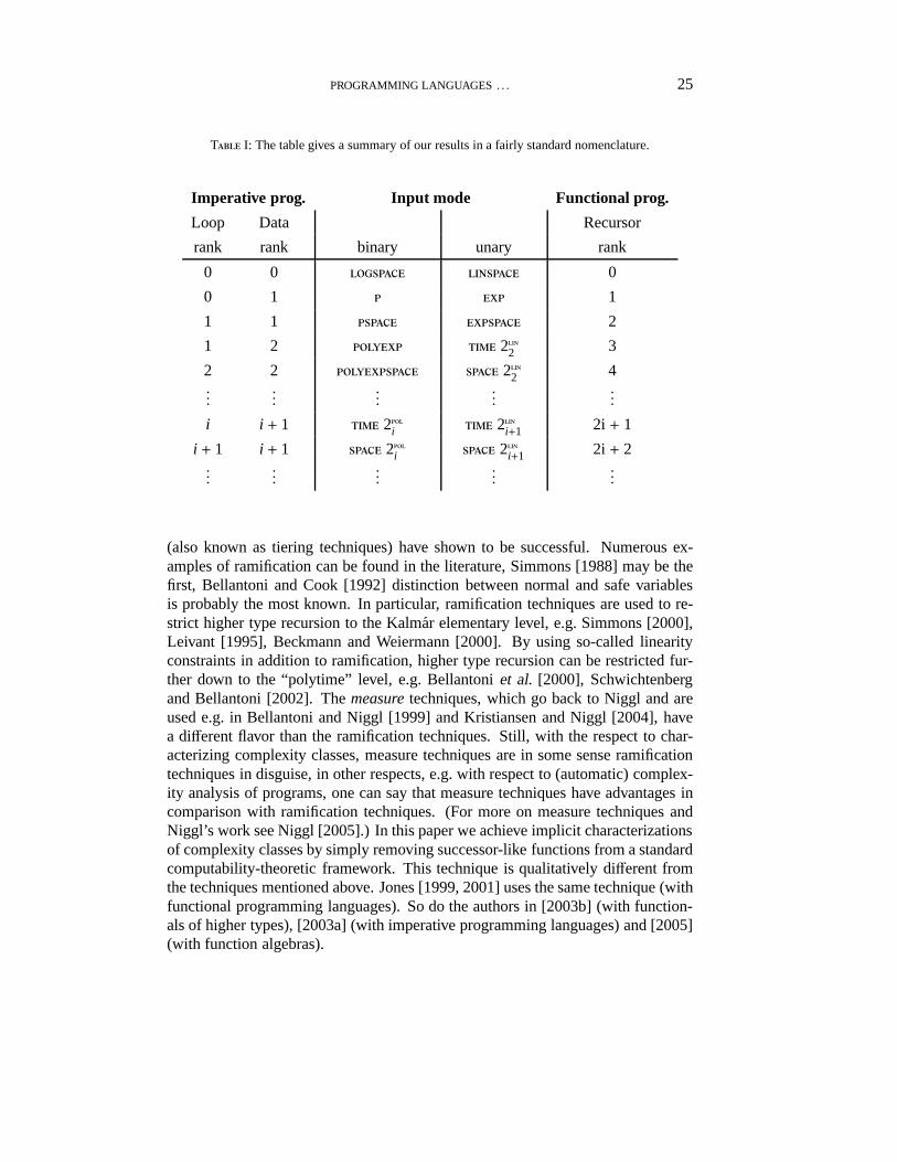
T 5. We have 2i = Ii+1,i+1

= F 2i+2 and 2i = Ii,i+1= F 2i+1

for any i∈ N. Moreover, we have = I0,0= F 0

We have not carried out all the technical details in the proofof Theorem 5, but wehave carried out quite a few details, and it is definitely possible to prove Theorem 5along the same lines as we have proved Theorem 1. The two proofs are essentiallythe same. Thus, we see that all the major deterministic complexity classes arecaptured by fragments of our programming languages. Table Igives a summary.

7. Discussion and References

7.1 Finite Model Theory and the Goerdt-Seidl Hierarchy

Goerdt and Seidl [1990] (and Goerdt [1992]) use finite modelsto characterize thealternating space-time hierarchy presented in Section 6. The inclusionsF 2i ⊆

2i andF 2i+1 ⊆ 2i+1 can be obtained directly from the theorems inGoerdt and Seidl [1990]. We hope that our proofs of the inclusions in Section 5are more enlightening and transparent than the corresponding proofs in Goerdt andSeidl [1990]. (Although it will be unfair to say that the proofs in Section 5 aresubstantially different from the ones in Goerdt and Seidl [1990]). The inclusions 2i ⊆ F

2i and 2i+1 ⊆ F2i+1 do not follow from Goerdt and Seidl’s work.

7.2 Implicit Characterizations of Complexity Classes

The characterizations of the complexity classes given by the two main theoremsof this paper are so-calledimplicit characterizations, that is, they contain no refer-ences to explicit resource bounds. To get rid of explicit resource bound and obtainimplicit characterizations of complexity classes, so-called ramification techniques


T I: The table gives a summary of our results in a fairly standard nomenclature.

Imperative prog. Input mode Functional prog.

Loop Data Recursor

rank rank binary unary rank

0 0 0

0 1 1

1 1 2

1 2 22 3

2 2 22 4...

......

......

i i + 1 2i 2i+1 2i + 1

i + 1 i + 1 2i 2i+1 2i + 2...

......

......

(also known as tiering techniques) have shown to be successful. Numerous ex-amples of ramification can be found in the literature, Simmons [1988] may be thefirst, Bellantoni and Cook [1992] distinction between normal and safe variablesis probably the most known. In particular, ramification techniques are used to re-strict higher type recursion to the Kalmar elementary level, e.g. Simmons [2000],Leivant [1995], Beckmann and Weiermann [2000]. By using so-called linearityconstraints in addition to ramification, higher type recursion can be restricted fur-ther down to the “polytime” level, e.g. Bellantoniet al. [2000], Schwichtenbergand Bellantoni [2002]. Themeasuretechniques, which go back to Niggl and areused e.g. in Bellantoni and Niggl [1999] and Kristiansen andNiggl [2004], havea different flavor than the ramification techniques. Still, with the respect to char-acterizing complexity classes, measure techniques are in some sense ramificationtechniques in disguise, in other respects, e.g. with respect to (automatic) complex-ity analysis of programs, one can say that measure techniques have advantages incomparison with ramification techniques. (For more on measure techniques andNiggl’s work see Niggl [2005].) In this paper we achieve implicit characterizationsof complexity classes by simply removing successor-like functions from a standardcomputability-theoretic framework. This technique is qualitatively different fromthe techniques mentioned above. Jones [1999, 2001] uses thesame technique (withfunctional programming languages). So do the authors in [2003b] (with function-als of higher types), [2003a] (with imperative programminglanguages) and [2005](with function algebras).


7.3 Product Types and the Small Grzegorczyk Classes

If we had left out explicit pairing and product types from thefunctional language,we could still prove that theF -hierarchy matches the alternating space-time hi-erarchy level by level with one exception. When explicit pairing is available, wecan prove thatF 0

= ; when it is not available, all we can prove is thatF 0= E0

∗ whereE0 is the 0’th Grzegorczyk class. It is known that = E2∗

whereE2 is the seconds Grzegorczyk class [Ritchie 1963]; it is not known if anyof the inclusionsE0

∗ ⊆ E1∗ ⊆ E

2∗ are strict. Kristiansen and Barra [2005] relate this

open problem to the research presented in this paper. They introduce a hierarchyL0⋆ ⊆ L

1⋆ ⊆ L

2⋆ ⊆ . . . whereL0

⋆ ⊆ E0∗ and

⋃

i∈NLi⋆ = E

2∗. The classes in the

hierarchy are induced by fragments of the typedλ-calculus extended by recursorsand the constant 1. For more on the small Grzegorczyk classessee Chapter 5 inRose [1984], Kutylowski [1987], Kristiansen and Barra [2005].

Acknowledgements

The authors want to thank G. Mathias Barra for useful comments and the Univer-sity of Copenhagen for hospitality.

References

A, J. F, S. 1998. Godel’s functional interpretation. InHandbook of Proof Theory,Buss, S., Editor. Elsevier.

B, A. 2001. Exact bounds for length reductions in typedλ-calculus.The Journal of Sym-bolic Logic 66, 3, 1277–1285.

B, A. W, A. 2000. Characterizing the elementary recursive functions by afragment of Godel’sT. Archive for Mathematical Logic 39, 4, 475–491.

B, S. J. C, S. 1992. A New Recursion-Theoretic Characterization of the PolytimeFunctions.Computational Complexity 2, 97–110.

B, S. J.N, K.-H. 1999. Ranking primitive recursions: The low Grzegorczyk classesrevisited.SIAM Journal on Computing 29, 2, 401–415.

B, S. J., N, K.-H., S, H. 2000. Higher type recursion, ramificationand polynomial time.Annals of Pure and Applied Logic 104, 17–30.

C, A. 1965. The intrinsic computational difficulty of functions. InLogic Methodology Philos.Sci., Proc. 1964 internat. Congr., 24–30.

F, R. 1974. Generalized first-order spectra and polynomial-time recognizable sets. InComplex-ity of Computation, Volume 7 ofSIAM-AMS Proceedings, 43–73.

G, A. 1992. Characterizing complexity classes by higher typeprimitive recursive definitions.Theoretical Computer Science 100, 1, 45–66.

G, A. S, H. 1990. Characterizing complexity classes by higher typeprimitive recursivedefinitions, Part II. InAspects and prospects of theoretical computer science, Volume 464 ofLecture Notes in Computer Science. Springer, 148–158.

J, N.D. 1997.Computability and Complexity from a Programming Perspective. Foundations ofComputing Series. MIT Press, Cambrigde, MA.

J, N.D. 1999. and characterized by programming languages.Theoretical Com-puter Science 228, 151–174.

J, N.D. 2001. The expressive power of higher-order types or, life without CONS. Journal ofFunctional Programming 11, 55–94.

K, L. 2005. Neat function algebraic characterizations ofLOGSPACEandLINSPACE.Computational Complexity 14, 1, 72–88.


K, L. B, G.M. 2005. The small Grzegorczyk classes and the typedλ-calculus.In CiE 2005: New Computational Paradigms, Volume 3526 ofLecture Notes in ComputerScience. Springer, 252–262.

K, L. N, K.-H. 2004. On the computational complexity of imperativeprogram-ming languages.Theoretical Computer Science 318, 139–161.

K, L. V, P.J. 2003a. Complexity classes and fragments of C.Information Process-ing Letters 88, 213–218.

K, L. V, P.J. 2003b. The surprising power of restricted programs and Godel’s func-tionals. InCSL 2003: Computer Science Logic, Volume 2803 ofLecture Notes in ComputerScience. Springer.

K, M. 1987. Small Grzegorczyk classes.Journal of the London Mathematical Society 36,2, 193–210.

L, D. 1995. Intrinsic theories and computational complexity. In Logic and ComputationalComplexity, Volume 960 ofLecture Notes in Computer Science. Springer, 177–194.

L, H. P, C.H. 1998.Elements of the theory of computation. Prentice-Hall.N, K-.H. 2005. Control Structures in Programs and Computational Complexity.Annals of Pure

and Applied Logic 133, 1-3, 247–273.O, P. 1999. Classical recursion theory. Vol. II. Volume 143 ofStudies in Logic and the

Foundations of Mathematics. North-Holland Publishing Co., Amsterdam.R, R. W. 1963. Classes of predictably computable functions.Transactions of the American

Mathematical Society 106, 139–173.R, H.E. 1984.Subrecursion. Functions and hierarchies. Clarendon Press.S, H. 1982. Complexity of normalization in the pure typedλ-calculus. InThe

L.E.J. Brouwer Centenary Symposium, Volume 110 ofStudies in Logic and the Foundationsof Mathematics. North-Holland, 453–457.

S, H. B, S.J. 2002. Feasible computation with higher types. InProofand System-Reliability.

S, H. 1988. The Realm of Primitive Recursion.Archive for Mathematical Logic 27, 177–188.S, H. 2000.Derivation and computation. Taking the Curry-Howard correspondence seriously.

Volume 51 ofCambridge Tracts in Theoretical Computer Science. Cambridge University Press.S, M.H.B. U, P. 2006. Lectures on the Curry-Howard Isomorphism. Elsevier

(to appear).

programming languages capturing complexity classesfolk.uio.no/larsk/njc.pdf · programming...

Documents