Computer Physics Communications 185 (2014) 407–414

Contents lists available at ScienceDirect

Computer Physics Communications

journal homepage: www.elsevier.com/locate/cpc

Program for quantum wave-packet dynamics withtime-dependent potentials

C.M. Dion a,∗, A. Hashemloo a, G. Rahali a,ba Department of Physics, Umeå University, SE-901 87 Umeå, Swedenb Department of Physics, Jazan University, Jazan, Saudi Arabia

a r t i c l e i n f o

Article history:Received 23 April 2013Received in revised form12 September 2013Accepted 17 September 2013Available online 29 September 2013

Keywords:Wave-packet dynamicsTime-dependent Schrödinger equationIon trapsLaser control

a b s t r a c t

We present a program to simulate the dynamics of a wave packet interacting with a time-dependentpotential. The time-dependent Schrödinger equation is solved on a one-, two-, or three-dimensional spa-tial grid using the split operator method. The program can be compiled for execution either on a singleprocessor or on a distributed-memory parallel computer.

Program summary

Program title: wavepacket

Catalogue identifier: AEQW_v1_0

Program summary URL: http://cpc.cs.qub.ac.uk/summaries/AEQW_v1_0.html

Program obtainable from: CPC Program Library, Queen’s University, Belfast, N. Ireland

Licensing provisions: Standard CPC licence, http://cpc.cs.qub.ac.uk/licence/licence.html

No. of lines in distributed program, including test data, etc.: 7231No. of bytes in distributed program, including test data, etc.: 232209Distribution format: tar.gzProgramming language: C (iso C99).

Computer: Any computer with an iso C99 compiler (e.g, gcc [1]).

Operating system: Any.Has the code been vectorized or parallelized?: Yes, parallelized using MPI. Number of processors: from 1 tothe number of grid points along one dimension.

RAM: Strongly dependent on problem size. See text for memory estimates.

Classification: 2.7.External routines: fftw [2], mpi (optional) [3]

Nature of problem:Solves the time-dependent Schrödinger equation for a single particle interacting with a time-dependentpotential.

Solution method:The wave function is described by its value on a spatial grid and the evolution operator is approximatedusing the split-operator method [4, 5], with the kinetic energy operator calculated using a Fast FourierTransform.

Unusual features:Simulation can be in one, two, or three dimensions. Serial and parallel versions are compiled from thesame source files.

This paper and its associated computer program are available via the Computer Physics Communication homepage on ScienceDirect (http://www.sciencedirect.com/science/journal/00104655).∗ Corresponding author. Tel.: +46 907865043.

E-mail address: claude.dion@physics.umu.se (C.M. Dion).

0010-4655/$ – see front matter© 2013 Elsevier B.V. All rights reserved.http://dx.doi.org/10.1016/j.cpc.2013.09.012

408 C.M. Dion et al. / Computer Physics Communications 185 (2014) 407–414

Running time:Strongly dependent on problem size. The example provided takes only a few minutes to run.References:

[1] http://gcc.gnu.org[2] http://www.fftw.org[3] http://www.mpi-forum.org[4] M.D. Feit, J.A. Fleck Jr., A. Steiger, Solution of the Schrödinger equation by a spectralmethod, J. Comput.

Phys. 47 (1982) 412–433.[5] M.D. Feit, J.A. Fleck Jr., Solution of the Schrödinger equation by a spectralmethod II: vibrational energy

levels of triatomic molecules, J. Chem. Phys. 78 (1) (1983) 301–308.

© 2013 Elsevier B.V. All rights reserved.

1. Introduction

Quantum wave-packet dynamics, that is, the evolution of thespatial distribution of a quantum particle, is an important part ofthe simulation of many quantum systems. It can be used for study-ing problems as diverse as scattering, surface adsorption, and lasercontrol, just to name a few.

We propose here a general-purpose program to solve thespatial part of the time-dependent Schrödinger equation (tdse),aimed particularly at a quantum particle interacting with a time-dependent potential. Our interest mainly concerns such applica-tions as laser control of quantum systems [1,2], but the programcan be used with any user-supplied potential function.

The program is based on the split-operator method [3–6],which has successfully been used to solve the time-dependentSchrödinger equation in many different settings, from the calcu-lation of vibrational bound states (see, e.g., [5]) and the simula-tion of high-power laser–matter interactions (see, e.g., [7]), to thelaser control of chemical reactions (see, e.g., [8]). The method canalso be applied to Schrödinger-like equations, such as the Gross–Pitaevskii [9] and Dirac [10] equations.

2. Numerical approach

2.1. Split-operator method

In this section, we present a detailed description of the split-operator method to solve the time-dependent Schrödinger equa-tion. While everything presented here can be found in the originalworks developing the method [3–6], we think it useful to reviewall the elements necessary to understand the inner workings of theprogram.

We consider the time-dependent Schrödinger equation,

ih∂

∂tψ(t) = Hψ(t), (1)

with H theHamiltonian for themotion of a particle interactingwithan external time-dependent potential V (t), i.e.,

H = K + V =P2

2m+ V (t), (2)

where K and V are the kinetic and potential energy operators, re-spectively, P is themomentumoperator, andm themass of the par-ticle. (The same Hamiltonian is obtained for a vibrating diatomicmolecule, where the spatial coordinate is replaced by the internu-clear distance, and the potential V (t) is the sum of the internal po-tential energy and an external, time-dependent potential, as willbe shown in Section 4.1.)

The formal solution to Eq. (1) is given by the time evolution op-erator U , itself a solution of the time-dependent Schrödinger equa-tion [11],

ih∂

∂tU = HU, (3)

such that, given an initial wave function at time t0, ψ(t0), the so-lution at any time t is obtained from

ψ(t) = U(t, t0)ψ(t0). (4)As the Hamiltonian is time dependent, we have that [12]

U(t, t0) = T exp−

ih

t

t0H(t ′)dt ′

= T exp

−

ih

t

t0

K + V (t ′)

dt ′

. (5)

In Eq. (5), the time-ordering operator T ensures that the Hamilto-nian is applied to the wave function in order of increasing time, asin general the Hamiltonian does not commute with itself at a dif-ferent time, i.e., [H(t), H(t ′)] = 0 iff t = t ′ [11,13]. By consideringa small time increment 1t , we can do without the time-orderingoperator by considering the approximate short-time evolution op-erator [13],

U(t +1t, t) = exp−

ih

t+1t

t

K + V (t ′)

dt ′

. (6)

We are concerned here with time-dependent potentials thatalso have a spatial dependence, V ≡ V (x, t), such as those pro-duced by ion traps or focused laser pulses, such that V ≡ V (x, t),in which case K and V do not commute. For two non-commutingoperators A and B, eA+B = eAeB, but the split-operatormethod [4,5]allows the approximation of the evolution operator with minimalerror,

U(t +1t, t) = exp−

i1t2h

Kexp

−

ih

t+1t

tV (t ′)dt ′

× exp

−

i1t2h

K+ O(1t3). (7)

Using themidpoint formula [14] for the integral of the potential, t+1t

tf (t ′)dt ′ = f (t +1t/2)1t + O(1t3), (8)

we get

U(t +1t, t)

≈ exp−

i1t2h

Kexp

−

i1th

Vt +

1t2

exp

−

i1t2h

K, (9)

where the global error is O(1t3). The choice of the order of the op-erators K and V in the above equations is arbitrary, but the choice

C.M. Dion et al. / Computer Physics Communications 185 (2014) 407–414 409

wemake here allows for a faster execution in themajority of cases,i.e., when the intermediate value of thewave function is not neededat all time steps.We can then link togethern consecutive time stepsinto

U(t + n1t, t) = U(t + n1t, t + [n− 1]1t)U(t

+[n− 1]1t, t + [n− 2]1t)× · · · × U(t +1t, t)

= exp−

i1t2h

Kexp

−

i1th

Vt +

2n− 12

1t

×

1

j=n−1

exp−

i1th

K

× exp−

i1th

Vt +

2j− 12

1t

exp−

i1t2h

K, (10)

where two sequential operations of K are combined into one. Thesame is not possible with V due to its time dependence.

We choose to discretize the problem on a finite spatial grid, i.e.,x = (x, y, z) is restricted to the values

xi = xmin + i1x, i = 0, . . . , nx − 1,yj = ymin + j1y, j = 0, . . . , ny − 1,

zk = zmin + k1z, k = 0, . . . , nz − 1, (11)

where the number of grid points (nx, ny, nz) are (integer) param-eters, as is the size of the grid, with bounds x ∈ [xmin, xmax] andwhere

1x =xmax − xmin

nx − 1, (12)

with equivalent expressions in y and z.The problem now becomes that of calculating the exponential

of matrices K and V, which is only trivial for a diagonal matrix [15].In the original implementation of the split-operator method [4,5],this is remedied by considering that while the matrix for V is diag-onal for a spatial representation of thewave function, K is diagonalin momentum space. By using a Fourier transform (here repre-sented by the operator F ) and its inverse (F −1), we can write

exp−

i1t2h

K(x)ψ(x) = F −1 exp

−

i1t2h

K(p)

F ψ(x), (13)

where, considering that K = P2/2m,

K(p) =p2

2m, (14)

K(x) = −h2

2m∇

2, (15)

since the operators transform as−ih∇ ⇔ p when going from po-sition tomomentum space [11]. Eq. (13) is efficiently implementednumerically using a Fast Fourier Transform (fft) [16]. After the for-ward transform, themomentum grid, obtained from thewave vec-tor k = p/h, is discretized according to [16]

px,i = 2π hi

nx1x, i = −

nx

2, . . . ,

nx

2,

py,j = 2π hj

ny1y, j = −

ny

2, . . . ,

ny

2,

pz,k = 2π hk

nz1z, k = −

nz

2, . . . ,

nz

2. (16)

Care must be taken to associate the appropriate momentum valueto each element of the Fourier-transformedwave function, consid-ering the order of the output from fft routines [16]. Algorithm 1summarizes the split-operator method as presented here.

Algorithm 1:Main algorithm for the split-operator method.Initialize ψ(t = 0)for j← 1 to nt/nprint doψ(p)← F ψ(x)

Multiply ψ(p) by exp−

i∆t2h

p22m

ψ(x)← F −1ψ(p)for i← 1 to nprint − 1 do

Multiply ψ(x) by exp−

i∆th V (x, t)

ψ(p)← F ψ(x)

Multiply ψ(p) by exp−

i∆th

p22m

ψ(x)← F −1ψ(p)

end

Multiply ψ(x) by exp−

i∆th V (x, t)

ψ(p)← F ψ(x)

Multiply ψ(p) by exp−

i∆t2h

p22m

ψ(x)← F −1ψ(p)Calculate observables ⟨A⟩ ≡ ⟨ψ(x)|A|ψ(x)⟩

end

2.2. Parallel implementation

We consider now the implementation of the algorithm de-scribed above on a multi-processor architecture with distributedmemory. The ‘‘natural’’ approach to parallelizing the problem is todivide the spatial grid, and therefore the wave function, among theprocessors. Each processor can work on its local slice of the wavefunction, except for the Fourier transform, which requires infor-mation across slices. This functionality is pre-built into the parallelimplementation of the fft package fftw [17], of whichwe take ad-vantage. The communications themselves are implemented usingthe Message Passing Interface (mpi) library [18,19].

For a 3D (or 2D) problem, the wave function is split along thex direction, with each processor having a subset of the grid in x,but with the full extent in y and z. To minimize the amount ofcommunication after the forward fft, we use the intermediatetransposed function, where the split is now along the y dimension.The original arrangement is recovered after the backward function,so this is transparent to the user of our program. In addition, fftwoffers the possibility of performing a 1D transform in parallel,which we also implement here.

The only constraint this imposes on the user is that a 1D prob-lemmay only be defined along x, and a 2D problem in the xy-plane(in order to simplify the concurrent implementation of serial andparallel versions, this constraint also applies to the serial version).In addition to the total number of grid points along x, nx, each pro-cessor has access to nx,local, the number of grid points in x for thisprocessor, along with nx,0, the corresponding initial index. In otherwords, each processor has a grid in x defined by

xi = xmin +i+ nx,0

1x, i = 0, . . . , nx,local, (17)

with the grids in y and z still defined by Eq. (11).

3. User guide

3.1. Summary of the steps for compilation and execution

Having defined the physical problem to be simulated, namelyby setting up the potential V (x, t) and initial wave function ψ(x;

410 C.M. Dion et al. / Computer Physics Communications 185 (2014) 407–414

t = 0), the following routines must be coded (see Section 3.2 fordetails):• initialize_potential• potential• initialize_wf• initialize_user_observe (can be empty)• user_observe (can be empty).

The files containing these functions must include the header filewavepacket.h. The program can then be compiled according tothe instructions in Section 3.3.

A parameter file must then be created, see Section 3.4. Theprogram can then be executed using a command similar towavepacket parameters.in

3.2. User-defined functions

The physical problem that is actually simulated by the programdepends on two principal elements, the time-dependent potentialV (x, t) and the initial wave function ψ(x; t = 0). In addition, theuser may be interested in observables that are not calculated bythe main program (the list a which is given in Section 3.4). Theusermust supply functionswhich define those elements,which arelinked to at compile time. How these functions are declared andwhat they are expected to perform is described in what follows,along with the data structure that is passed to those functions.

3.2.1. Data structure parametersThe data structure parameters is defined in the header file

wavepacket.h, which must be included at the top of the usersown C files to be linked to the program. A variable of typeparameters is passed to the user’s functions, and contains allparameters the main program is aware of and that are useful/necessary for the execution of the tasks of the user-supplied rou-tines. The structure readstypedef struct

/* Parameters and grid */int size, rank;size_t nx, ny, nz, n, nx_local, nx0, n_local;double x_min, y_min, z_min, x_max, y_max, z_max, dx, dy, dz;double *x, *y, *z, *x2, *y2, *z2;double mass, dt, hbar;

parameters;

where the different variables are:• size: Number of processors on which the program is running.• rank: Rank of the local processor, with a value in the range[0, size− 1]. In the serial version, the value is therefore rank= 0. (Note: All input and output to/from disk is performed bythe processor of rank 0.)• nx, ny, nz: Number of grid points along x, y, and z, respec-

tively. In the parallel version, this refers to the full grid, which isthen split among the processors. For a one or two-dimensionalproblem, ny and/or nz should be set to 1. (x is always the prin-cipal axis in the program.) For best performance, these shouldbe set to a product of powers of small prime integers, e.g.,

nx = 2i3j5k7l.

See the documentation of fftw for more details [20].• n = nx× ny× nz.• nx_local: Number of grid points in x on the local processor,

see Section 2.2. In the serial version, nx_local = nx.• nx0: Index of the first local grid point in x, see Section 2.2. In

the serial version, nx0 = 0.• x_min, y_min, z_min, x_max, y_max, z_max: Values

of the first and last grid points along x, y, and z.• dx, dy, dz: Grid spacings1x,1y, and1z, respectively, see

Eq. (12).

• x, y, z: Arrays of size nx_local, ny, and nz, respectively, con-taining the value of the corresponding coordinate at the gridpoint.• x2, y2, z2: Arrays of size nx_local, ny, and nz, respectively,

containing the square of the value of the corresponding coordi-nate at the grid point.• mass: Mass of the particle.• dt: Time step1t of the time evolution, see Eq. (6).• hbar: Value of h, Planck’s constant over 2π , in the proper units.

(See Section 3.4.)

3.2.2. Initializing the potentialIn the initialization phase of the program, before the time

evolution, the functionvoidinitialize_potential (const parameters params, const int argv,

char ** const argc);

is called, with the constant variable params containing all thevalues specified in Section 3.2.1. argv and argc are the variablesrelating to the command line arguments, as passed to the mainprogram:intmain (int argv, char **argc);

This function should perform all necessary pre-calculations andoperations, including reading from a file additional parameters,for the potential function. The objective is to reduce as most aspossible the time necessary for a call to the potential function.

3.2.3. Potential functionThe function

doublepotential (const parameters params, const double t,

double * const pot);

should return the value of the potential V (x, t), for all (local) gridpoints at time t, in the array pot, of dimension pot[nx_local][ny][nz].

3.2.4. Initial wave functionThe initial wave function ψ(x, t = 0) is set by the function

voidinitialize_wf (const parameters params, const int argv,

char ** const argc, double complex *psi);

where psi is a 3D array of dimension psi[nx_local][ny][nz]. If the wave function is to be read from a file, users canmake use of the functionsread_wf_text andread_wf_bin, de-scribed in Section 3.2.6.

3.2.5. User-defined observablesIn addition to the observables that are built in, which are

described in Section 3.4, users may define additional observables,such as the projection of the wave function on eigenstates.

The functionvoidinitialize_user_observe (const parameters params, const int argc,

char ** const argv);

is called once at the beginning of the execution. It should per-form all operations needed before any call to user_observe.The arguments passed to the function are the same as those ofinitialize_potential, see Section 3.2.2.

During the time evolution, every nprint time step, thefunctionvoiduser_observe (const parameters params, const double t,

const double complex * const psi);

is called, with the current time t and wave function psi.

C.M. Dion et al. / Computer Physics Communications 185 (2014) 407–414 411

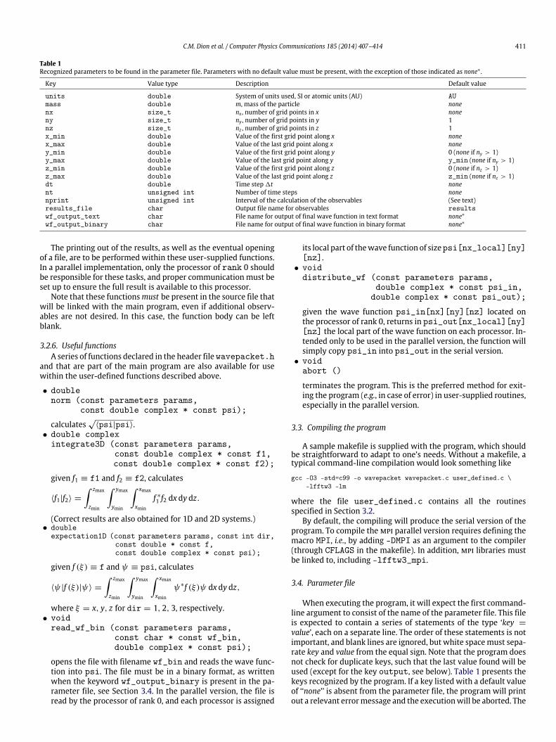
Table 1Recognized parameters to be found in the parameter file. Parameters with no default value must be present, with the exception of those indicated as none∗ .

Key Value type Description Default value

units double System of units used, SI or atomic units (AU) AUmass double m, mass of the particle nonenx size_t nx , number of grid points in x noneny size_t ny , number of grid points in y 1nz size_t nz , number of grid points in z 1x_min double Value of the first grid point along x nonex_max double Value of the last grid point along x noney_min double Value of the first grid point along y 0 (none if ny > 1)y_max double Value of the last grid point along y y_min (none if ny > 1)z_min double Value of the first grid point along z 0 (none if nz > 1)z_max double Value of the last grid point along z z_min (none if nz > 1)dt double Time step1t nonent unsigned int Number of time steps nonenprint unsigned int Interval of the calculation of the observables (See text)results_file char Output file name for observables resultswf_output_text char File name for output of final wave function in text format none∗wf_output_binary char File name for output of final wave function in binary format none∗

The printing out of the results, as well as the eventual openingof a file, are to be performed within these user-supplied functions.In a parallel implementation, only the processor of rank 0 shouldbe responsible for these tasks, and proper communication must beset up to ensure the full result is available to this processor.

Note that these functionsmust be present in the source file thatwill be linked with the main program, even if additional observ-ables are not desired. In this case, the function body can be leftblank.

3.2.6. Useful functionsA series of functions declared in the header file wavepacket.h

and that are part of the main program are also available for usewithin the user-defined functions described above.

• doublenorm (const parameters params,

const double complex * const psi);

calculates√⟨psi|psi⟩.

• double complexintegrate3D (const parameters params,

const double complex * const f1,const double complex * const f2);

given f1 ≡ f1 and f2 ≡ f2, calculates

⟨f1|f2⟩ = zmax

zmin

ymax

ymin

xmax

xmin

f ∗1 f2 dx dy dz.

(Correct results are also obtained for 1D and 2D systems.)• double

expectation1D (const parameters params, const int dir,const double * const f,const double complex * const psi);

given f (ξ) ≡ f and ψ ≡ psi, calculates

⟨ψ |f (ξ)|ψ⟩ = zmax

zmin

ymax

ymin

xmax

xmin

ψ∗f (ξ)ψ dx dy dz,

where ξ = x, y, z for dir = 1, 2, 3, respectively.• voidread_wf_bin (const parameters params,

const char * const wf_bin,double complex * const psi);

opens the file with filename wf_bin and reads the wave func-tion into psi. The file must be in a binary format, as writtenwhen the keyword wf_output_binary is present in the pa-rameter file, see Section 3.4. In the parallel version, the file isread by the processor of rank 0, and each processor is assigned

its local part of thewave function of sizepsi[nx_local][ny][nz].• voiddistribute_wf (const parameters params,

double complex * const psi_in,double complex * const psi_out);

given the wave function psi_in[nx][ny][nz] located onthe processor of rank 0, returns in psi_out[nx_local][ny][nz] the local part of the wave function on each processor. In-tended only to be used in the parallel version, the function willsimply copy psi_in into psi_out in the serial version.• voidabort ()

terminates the program. This is the preferred method for exit-ing the program (e.g., in case of error) in user-supplied routines,especially in the parallel version.

3.3. Compiling the program

A sample makefile is supplied with the program, which shouldbe straightforward to adapt to one’s needs. Without a makefile, atypical command-line compilation would look something like

gcc -O3 -std=c99 -o wavepacket wavepacket.c user_defined.c \-lfftw3 -lm

where the file user_defined.c contains all the routinesspecified in Section 3.2.

By default, the compiling will produce the serial version of theprogram. To compile thempi parallel version requires defining themacro MPI, i.e., by adding -DMPI as an argument to the compiler(through CFLAGS in the makefile). In addition, mpi libraries mustbe linked to, including -lfftw3_mpi.

3.4. Parameter file

When executing the program, it will expect the first command-line argument to consist of the name of the parameter file. This fileis expected to contain a series of statements of the type ‘key =value’, each on a separate line. The order of these statements is notimportant, and blank lines are ignored, but white spacemust sepa-rate key and value from the equal sign. Note that the program doesnot check for duplicate keys, such that the last value found will beused (except for the key output, see below). Table 1 presents thekeys recognized by the program. If a key listed with a default valueof ‘‘none’’ is absent from the parameter file, the program will printout a relevant errormessage and the executionwill be aborted. The

412 C.M. Dion et al. / Computer Physics Communications 185 (2014) 407–414

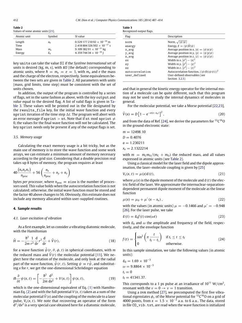
Table 2Values of some atomic units [21].

Atomic unit Symbol SI value

Length a0 0.529 177 210 92× 10−10 mTime 2.418 884 326 502× 10−17 sMass me 9.109 382 91× 10−31 kgEnergy Eh 4.359 744 34× 10−18 J

key units can take the value SI if the Système International set ofunits is desired (kg, m, s), with AU (the default) corresponding toatomic units, where h = me = e = 1, with me and e the massand the charge of the electron, respectively. Some equivalences be-tween the two sets are given in Table 2. All parameters with units(mass, grid limits, time step) must be consistent with the set ofunits chosen.

In addition, the output of the program is controlled by a seriesof flags, set in the same fashion as above, with the key output andvalue equal to the desired flag. A list of valid flags is given in Ta-ble 3. These values will be printed out in the file designated bythe results_file key, for the initial wave function and everynprint iteration of the time step1t . The programwill abort withan error message if nprint > nt. Note that if nt mod nprint =0, the values for the final wave function will not be calculated. Thekey nprint needs only be present if any of the output flags is set.

3.5. Memory usage

Calculating the exact memory usage is a bit tricky, but as themain use of memory is to store the wave function and some workarrays, we can estimate a minimum amount of memory necessaryaccording to the grid size. Considering that a double precision realtakes up 8 bytes of memory, the program requires at least

40

nxnynz

nproc

+ 56

nx

nproc+ ny + nz

bytes per processor, where nproc ≡ size is the number of proces-sors used. This value holdswhen the autocorrelation function is notcalculated; otherwise, the initial wave functionmust be stored andthe factor 40 above changes to 56. Obviously, this estimate does notinclude any memory allocated within user-supplied routines.

4. Sample results

4.1. Laser excitation of vibration

As a first example, let us consider a vibrating diatomicmolecule,with the Hamiltonian

H = −h2

2m1r2

ddr

r2ddr+ V (r), (18)

for a wave function ψ(r, θ, φ, t) in spherical coordinates, with mthe reduced mass and V (r) the molecular potential [11]. We ne-glect here the rotation of the molecule, and only look at the radialpart of the wave function, ψ(r, t). Setting ψ ≡ rψ , and substitut-ing x for r , we get the one-dimensional Schrödinger equation

ih∂

∂tψ(x, t) =

−

h2

2md2

dx2+ V (x, t)

ψ(x, t), (19)

which is the one-dimensional equivalent of Eq. (1) with Hamilto-nian Eq. (2) andwith the full potential V (x, t) taken as a sum of themolecular potential V (x) and the coupling of themolecule to a laserpulse, VL(x, t). We note that recovering an operator of the formd2/dx2 is a very special case obtained here for a diatomicmolecule,

Table 3Recognized output flags.

Flag Description

norm Norm,√⟨ψ |ψ⟩

energy Energy, E = ⟨ψ |H|ψ⟩x_avg Average position in x, ⟨x⟩ = ⟨ψ |x|ψ⟩y_avg Average position in y, ⟨y⟩ = ⟨ψ |y|ψ⟩z_avg Average position in z, ⟨z⟩ = ⟨ψ |z|ψ⟩sx Width in x,

x2

− ⟨x⟩2

sy Width in y,y2

− ⟨y⟩2

sz Width in z,z2

− ⟨z⟩2

autocorrelation Autocorrelation function, |⟨ψ(0)|ψ(t)⟩|2

user_defined User-defined observables (seeSection 3.2.5)

and that in general the kinetic energy operator for the internal mo-tion of a molecule can be quite different, such that this programmay not be used to study the internal dynamics of molecules ingeneral.

For the molecular potential, we take a Morse potential [22,23],

V (x) = D1− e−a(x−xe)

2, (20)

and from the data of Ref. [24], we derive the parameters for 12C16Oin the ground electronic state:

m = 12498.10D = 0.4076a = 1.230211xe = 2.1322214

with m = mCmO/(mC + mO) the reduced mass, and all valuesexpressed in atomic units (see Table 2).

Using a classical model for the laser field and the dipole approx-imation, the laser–molecule coupling is given by [25]

VL(x, t) = µ(x)E(t), (21)

whereµ(x) is the dipolemoment of themolecule andE(t) the elec-tric field of the laser.We approximate the internuclear-separation-dependent permanent dipolemoment of themolecule as the linearfunction

µ(x) = µ0 + µ′ (x− xe) , (22)

with the values (in atomic units) µ = −0.1466 and µ′ = −0.948[26]. For the laser pulse, we take

E(t) = E0f (t) cos(ωt) (23)

with E0 and ω the amplitude and frequency of the field, respec-tively, and the envelope function

f (t) =

sin2π

ttf − ti

if ti ≤ t ≤ tf

0 otherwise.(24)

In this sample simulation, we take the following values (in atomicunits):

E0 = 1.69× 10−3

ω = 9.8864× 10−3

ti = 0tf = 41341.37.

This corresponds to a 1 ps pulse at an irradiance of 1011 W/cm2,resonant with the v = 0→ v = 1 transition.

Using a dvr method [27], we precomputed the first five vibra-tional eigenstates φv of the Morse potential for 12C16O on a grid of4000 points, from x = 1.5 × 10−3 a.u. to 6 a.u.. The data, storedin file CO_vib.txt, are readwhen the wave function is initialized

C.M. Dion et al. / Computer Physics Communications 185 (2014) 407–414 413

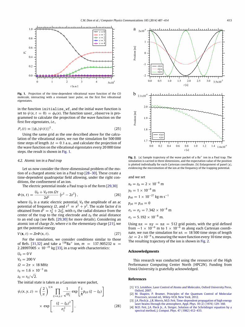
Fig. 1. Projection of the time-dependent vibrational wave function of the COmolecule, interacting with a resonant laser pulse, on the first five vibrationaleigenstates.

in the function initialize_wf, and the initial wave function isset to ψ(x, t = 0) = φ0(x). The function user_observe is pro-grammed to calculate the projection of the wave function on thefirst five eigenstates, i.e.,

Pv(t) ≡ |⟨φv|ψ(t)⟩|2 . (25)Using the same grid as the one described above for the calcu-

lation of the vibrational states, we run the simulation for 500 000time steps of length1t = 0.1 a.u., and calculate the projection ofthewave function on the vibrational eigenstates every 20 000 timesteps. the result is shown in Fig. 1.

4.2. Atomic ion in a Paul trap

Let us now consider the three-dimensional problem of the mo-tion of a charged atomic ion in a Paul trap [28–30]. These create atime-dependent quadrupolar field allowing, under the right con-ditions, the confinement of an ion.

The electric potential inside a Paul trap is of the form [29,30]

Φ(x, t) =U0 + V0 cosΩt

2d2r2 − 2z2

, (26)

where U0 is a static electric potential, V0 the amplitude of an acpotential of frequency Ω , and r2 ≡ x2 + y2. The scale factor d isobtained from d2 = r20 + 2z20 , with r0 the radial distance from thecenter of the trap to the ring electrode and z0 the axial distanceto an end cap (see Refs. [29,30] for more details). Considering anatomic ion of charge Ze, where e is the elementary charge [21], weget the potential energyV (x, t) = ZeΦ(x, t). (27)

For the simulation, we consider conditions similar to thoseof Refs. [31,32] and take a 138Ba+ ion, m = 137.905232 u =2.28997005× 10−25 kg [33], in a trap with characteristics:U0 = 0 VV0 = 200 VΩ = 2π × 18 MHzr0 = 1.6× 10−3 m

z0 = r0/√2.

The initial state is taken as a Gaussian wave packet,

ψi(x, y, z) =

2π

3/4 ξ=x,y,z

1√σξ

expihpξ0 (ξ − ξ0)

× exp

−(ξ − ξ0)

2

σ 2ξ

, (28)

a

b

Fig. 2. (a) Sample trajectory of the wave packet of a Ba+ ion in a Paul trap. Thesimulation is carried in three dimensions, and the expectation value of the positionis plotted individually for each Cartesian coordinate. (b) Enlargement of panel (a),evidencing the micromotion of the ion at the frequency of the trapping potential.

and we set

x0 = z0 = 2× 10−8 m

y0 = 1× 10−8 m

px0 = 1× 10−27 kg m s−1

py0 = pz0 = 0

σx = σy = 7.342× 10−8 m

σz = 5.192× 10−8 m.

Using nx = ny = nz = 512 grid points, with the grid definedfrom −1 × 10−6 m to 1 × 10−6 m along each Cartesian coordi-nate, we run the simulation for nt = 18 500 time steps of length1t = 2×10−9 s,measuring thewave function every 10 time steps.The resulting trajectory of the ion is shown in Fig. 2.

Acknowledgments

This research was conducted using the resources of the HighPerformance Computing Center North (HPC2N). Funding fromUmeå University is gratefully acknowledged.

References

[1] V.S. Letokhov, Laser Control of Atoms and Molecules, Oxford University Press,Oxford, 2007.

[2] M. Shapiro, P. Brumer, Principles of the Quantum Control of MolecularProcesses, second ed., Wiley-VCH, New York, 2012.

[3] J.A. Fleck Jr., J.R. Morris, M.D. Feit, Time-dependent propagation of high energylaser beams through the atmosphere, Appl. Phys. 10 (2) (1976) 129–160.

[4] M.D. Feit, J.A. Fleck Jr., A. Steiger, Solution of the Schrödinger equation by aspectral method, J. Comput. Phys. 47 (1982) 412–433.

414 C.M. Dion et al. / Computer Physics Communications 185 (2014) 407–414

[5] M.D. Feit, J.A. Fleck Jr., Solution of the Schrödinger equation by a spectralmethod II: vibrational energy levels of triatomic molecules, J. Chem. Phys. 78(1) (1983) 301–308.

[6] A.D. Bandrauk, H. Shen, Improved exponential split operator method forsolving the time-dependent Schrödinger equation, Chem. Phys. Lett. 176 (5)(1991) 428–432.

[7] Y.I. Salamin, S. Hu, K.Z. Hatsagortsyan, C.H. Keitel, Relativistic high-powerlaser–matter interactions, Phys. Rep. 427 (2–3) (2006) 41–155.

[8] C.M. Dion, S. Chelkowski, A.D. Bandrauk, H. Umeda, Y. Fujimura, Numericalsimulation of the isomerization of HCN by two perpendicular intense IR laserpulses, J. Chem. Phys. 105 (1996) 9083–9092.

[9] J. Javanainen, J. Ruostekoski, Symbolic calculation in development ofalgorithms: split-step methods for the Gross–Pitaevskii equation, J. Phys. A 39(2006) L179–L184.

[10] G.R.Mocken, C.H. Keitel, FFT-split-operator code for solving the Dirac equationin 2+1 dimensions, Comput. Phys. Comm. 178 (11) (2008) 868–882.

[11] C. Cohen-Tannoudji, B. Diu, F. Laloë, Quantum Mechanics, Wiley, New York,1992.

[12] H.-P. Breuer, F. Petruccione, The Theory of Open Quantum Systems, OxfordUniversity Press, Oxford, 2002.

[13] P. Pechukas, J.C. Light, On the exponential form of time-displacementoperators in quantum mechanics, J. Chem. Phys. 44 (10) (1966) 3897–3912.

[14] S.D. Conte, C. de Boor, Elementary Numerical Analysis, second ed., McGraw-Hill, 1972.

[15] C. Moler, C. Van Loan, Nineteen dubious ways to compute the exponential of amatrix, twenty-five years later, SIAM Rev. 45 (1) (2003) 3–49.

[16] W.H. Press, S.A. Teukolsky,W.T. Vetterling, B.P. Flannery, Numerical Recipes inC, second ed., Cambridge University Press, Cambridge, 1992.

[17] M. Frigo, S.G. Johnson, The design and implementation of FFTW3, Proc. IEEE 93(2) (2005) 216–231. Special issue on ‘‘Program Generation, Optimization, andPlatform Adaptation’’.

[18] URL: http://www.mpi-forum.org/.

[19] W. Gropp, E. Lusk, A. Skjellum, UsingMPI: Portable Parallel Programmingwiththe Message Passing Interface, MIT Press, Cambridge, MA, 1999.

[20] URL: http://www.fftw.org/.[21] URL: http://physics.nist.gov/constants.[22] P.M. Morse, Diatomic molecules according to the wave mechanics, II.

Vibrational levels, Phys. Rev. 34 (1929) 57–64.[23] P. Atkins, R. Friedman, Molecular Quantum Mechanics, fifth ed., Oxford

University Press, Oxford, 2011.[24] K.P. Huber, G. Herzberg, Molecular Spectra and Molecular Structure: IV.

Constans of Diatomic Molecules, Van Nostrand Reinhold, New York, 1979.[25] A.D. Bandrauk (Ed.), Molecules in Laser Fields, Dekker, New York, 1994.[26] J.E. Gready, G.B. Bacskay, N.S. Hush, Finite-field method calculations, IV.

Higher-ordermoments, dipolemoment gradients, polarisability gradients andfield-induced shifts in molecular properties: application to N2 , CO, CN− , HCNand HNC, Chem. Phys. 31 (1978) 467–483.

[27] D.T. Colbert,W.H.Miller, A novel discrete variable representation for quantummechanical reactive scattering via the s-matrix Kohn method, J. Chem. Phys.96 (1992) 1982–1991.

[28] W. Paul, Electromagnetic traps for charged and neutral particles, Rev. ModernPhys. 62 (3) (1990) 531–540.

[29] F.G. Major, V.N. Gheorghe, G. Werth, Charged Particle Traps: Physics andTechniques of Charged Particle Field Confinement, Springer, Berlin, 2005.

[30] G. Werth, V.N. Gheorghe, F.G. Major, Charged Particle Traps II: Applications,Springer, Berlin, 2009.

[31] W. Neuhauser, M. Hohenstatt, P. Toschek, H. Dehmelt, Optical-sidebandcooling of visible atom cloud confined in parabolic well, Phys. Rev. Lett. 41(1978) 233–236.

[32] W. Neuhauser, M. Hohenstatt, P. Toschek, H. Dehmelt, Visual observation andoptical cooling of electrodynamically contained ions, Appl. Phys. 17 (1978)123–129.

[33] NIST handbook of basic atomic spectroscopic data. URL: http://www.nist.gov/pml/data/handbook/.