processing modflow x - simcore software · introduction 1.1. what is processing modflow processing...
TRANSCRIPT
Processing Modflow X
June 19, 2018
Copyright © 1991- 2018 Simcore Software

I
Contents Acknowledgements .......................................................................................................................... v
Application and Data Folders ........................................................................................................... v
Abbreviations .................................................................................................................................. vi
Image of the Start Window ............................................................................................................. vi
Supported MODFLOW Packages.................................................................................................... vii
Variables........................................................................................................................................ viii
Chapter 1. Introduction .............................................................................................................. 1
1.1. What is Processing Modflow ............................................................................................ 1
1.2. Main Window of PM ........................................................................................................ 2
Chapter 2. Maps.......................................................................................................................... 7
2.1. Views ................................................................................................................................ 7
2.2. Captions ............................................................................................................................ 8
2.3. Images .............................................................................................................................. 9
2.4. Base Maps ...................................................................................................................... 10
2.4.1. Edit Base Maps ........................................................................................................ 10
2.4.2. Customize the Display of a Base Map ..................................................................... 12
2.5. Shapefiles ....................................................................................................................... 12
2.5.1. Add Shapefiles to the Map Viewer ......................................................................... 12
2.5.2. Customize the Display of a Shapefile ...................................................................... 13
Chapter 3. Modeling Environment ........................................................................................... 17
3.1. Units ............................................................................................................................... 17
3.2. Temporal Discretization ................................................................................................. 17
3.3. Spatial Discretization ...................................................................................................... 17
3.3.1. Grid Editor ............................................................................................................... 18
3.3.2. Data Editor .............................................................................................................. 19
3.4. File Menu ........................................................................................................................ 28
3.4.1. New ......................................................................................................................... 28
3.4.2. Open ........................................................................................................................ 28
3.4.3. Recent Files ............................................................................................................. 28
II
3.4.4. Save ......................................................................................................................... 28
3.4.5. Save As .................................................................................................................... 28
3.4.6. Create Model .......................................................................................................... 28
3.4.7. Import Model .......................................................................................................... 32
3.4.8. Save Image .............................................................................................................. 34
3.4.9. Animation ................................................................................................................ 35
3.4.10. Print ..................................................................................................................... 36
3.4.11. Preferences ......................................................................................................... 36
3.5. Tools Menu ..................................................................................................................... 40
3.5.1. Pan Tool .................................................................................................................. 40
3.5.2. Zoom Tool ............................................................................................................... 41
3.5.3. Observation Tool ..................................................................................................... 41
3.5.4. MODPATH Tool ....................................................................................................... 43
3.5.5. Measure Tool .......................................................................................................... 44
3.5.6. Row Cross Section Tool ........................................................................................... 45
3.5.7. Pin Tool ................................................................................................................... 47
3.5.8. Rotation Tool........................................................................................................... 47
3.5.9. Finish Edit ................................................................................................................ 47
3.5.10. Cell-by-Cell Tool ................................................................................................... 47
3.5.11. Polyline Tool ........................................................................................................ 47
3.5.12. Polygon Tool ........................................................................................................ 47
3.5.13. Cell Copy .............................................................................................................. 47
3.5.14. Layer Copy ........................................................................................................... 47
3.5.15. Grid Size Copy ...................................................................................................... 48
3.5.16. Grid Split Copy ..................................................................................................... 48
3.5.17. Tools > Data Menu .............................................................................................. 48
3.5.18. Tools > Package Menu ......................................................................................... 53
3.6. Discretization Menu ....................................................................................................... 54
3.6.1. Time ........................................................................................................................ 54
3.6.2. Grid .......................................................................................................................... 56
3.6.3. Layer Property ......................................................................................................... 56
III
3.6.4. Layer Top Elevation and Layer Bottom Elevation ................................................... 60
3.6.5. IBOUND (Flow) ........................................................................................................ 60
3.6.6. ICBUND (Transport) ................................................................................................ 60
3.7. Parameters Menu ........................................................................................................... 61
3.7.1. Starting Hydraulic Head .......................................................................................... 61
3.7.2. Horizontal Hydraulic Conductivity (HK) and Transmissivity (T) .............................. 61
3.7.3. Horizontal Anisotropy (HANI) ................................................................................. 61
3.7.4. Vertical Hydraulic Conductivity (VK) and Vertical Leakance (VCONT) .................... 62
3.7.5. Vertical Anisotropy (VANI) ...................................................................................... 62
3.7.6. Specific Storage (Ss) and Storage Coefficient (S) .................................................... 62
3.7.7. Specific Yield (Sy) .................................................................................................... 63
3.7.8. Effective Porosity (ne) ............................................................................................. 63
3.7.9. Stop Zone ................................................................................................................ 63
3.7.10. Retardation Factor (R) ......................................................................................... 63
3.7.11. Bulk Density ......................................................................................................... 64
3.7.12. Static Sandboxes ................................................................................................. 64
3.7.13. Transient Sandboxes ........................................................................................... 64
3.8. Models Menu ................................................................................................................. 64
3.8.1. MODFLOW .............................................................................................................. 64
3.8.2. ZoneBudget ........................................................................................................... 136
3.8.3. MT3D/SEAWAT ..................................................................................................... 137
3.8.4. PEST ....................................................................................................................... 162
Chapter 4. Visualization and Postprocessing .......................................................................... 185
4.1. Input Data ..................................................................................................................... 185
4.1.1. Model Grid ............................................................................................................ 185
4.1.2. Packages ................................................................................................................ 186
4.1.3. Observation Points ................................................................................................ 187
4.2. Visualization ................................................................................................................. 188
4.2.1. Input Parameter Contours .................................................................................... 188
4.2.2. Result Contours ..................................................................................................... 192
4.2.3. Flow Vectors.......................................................................................................... 194
IV
4.2.4. MODPATH Instances ............................................................................................. 197
Chapter 5. Supplementary Information ................................................................................. 203
5.1. File Formats .................................................................................................................. 203
5.1.1. 2D Matrix and 2D Weight Matrix .......................................................................... 203
5.1.2. 2D Modflow Array ................................................................................................. 203
5.1.3. 3D Modflow Array ................................................................................................. 204
5.1.4. Comma-Separated Values File .............................................................................. 204
5.1.5. ESRI ASCII Raster ................................................................................................... 205
5.1.6. ESRI Shapefile ........................................................................................................ 205
5.1.7. MODPATH Starting Points..................................................................................... 205
5.1.8. Georeference file .................................................................................................. 206
5.1.9. Observation File .................................................................................................... 207
5.1.10. Polygon File ....................................................................................................... 208
5.1.11. Polyline File ....................................................................................................... 212
5.1.12. Reservoir Stage Time Series .............................................................................. 218
5.1.13. Series File ........................................................................................................... 218
5.1.14. SURFER ASCII GRD File ...................................................................................... 219
5.1.15. Temporal Discretization File.............................................................................. 219
5.1.16. Well File ............................................................................................................. 220
5.2. Input and Output Data Files of the Supported Models ............................................... 221
5.2.1. MODFLOW-2005/MODFLOW-NWT ...................................................................... 221
5.2.2. MT3DMS/MT3D-USGS .......................................................................................... 222
5.2.3. SEAWAT ................................................................................................................. 223
5.2.4. MODPATH ............................................................................................................. 223
5.2.5. PEST ....................................................................................................................... 223
References .................................................................................................................................. 226
Index ............................................................................................................................................ 231
V
Acknowledgements
We wish to express our sincere gratitude and appreciation to many people who have developed
the model codes, Open Source programming libraries, and online resources. This work would not
be possible without their generous contributions.
Application and Data Folders
The following folders will be created and used by Processing Modflow.
Application Files
Per-user installation (with pmx64_10.0.xx.exe or pmx32_10.0.xx.exe):
C:\Users\YourUserName\AppData\Local\Simcore Software\Processing Modflow 10
Per-machine installation (with pmx64admin_10.0.xx.exe) for all users:
C:\Program Files\Simcore Software\Processing Modflow X
Per-machine installation (with pmx32admin_10.0.xx.exe) for all users:
C:\Program Files (x86)\Simcore Software\Processing Modflow X
Application Cache and Temporary Files:
C:\Users\YourUserName\AppData\Simcore Software\Processing Modflow
Examples:
C:\Users\YourUserName\Documents\My Processing Modflow Models

VI
Abbreviations
CSV File: A comma-separated values file stores tabular data (numbers and text) in plain text. Each line of the file is a data record. Each record consists of one or more fields, separated by commas.
Ctrl-click: Place the mouse pointer to an object; press and hold down the Ctrl key; then press and release the (left) mouse button.
Shift-click: Place the mouse pointer to an object; press and hold down the Shift key; then press and release the (left) mouse button.
Drag and drop or drag: Move the mouse pointer to an object; press and hold down the left mouse button; drag the object to the desired location by moving the mouse pointer; then drop the object by releasing the left mouse button.
PM: Processing Modflow.
TOC: The Table of Contents window that is a part of the main window of Processing Modflow X. TOC contains a list of predefined groups; each group may contain user-defined objects.
UTC: Coordinated Universal Time.
UTM: Universal Transverse Mercator.
WGS 84: World Geodetic System 1984.
Image of the Start Window
The image of the Start Window of
Processing Modflow shows a small
section of the expanding remains of a
massive star that exploded about 8,000
years ago. Called the Veil Nebula, the
debris is one of the best-known
supernova remnants, deriving its name
from its delicate, draped filamentary
structures. The entire nebula is 110
light-years across, covering six full
moons on the sky as seen from Earth,
and resides about 2,100 light-years
away in the constellation Cygnus, the Swan.
Image Credit: NASA/ESA/Hubble Heritage Team. Source: https://www.nasa.gov/image-
feature/veil-nebula-supernova-remnant
VII
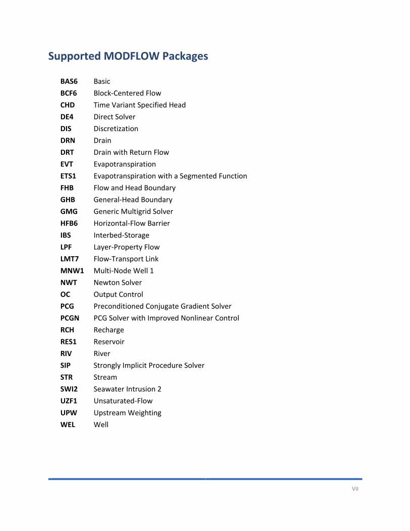
Supported MODFLOW Packages
BAS6 Basic
BCF6 Block-Centered Flow
CHD Time Variant Specified Head
DE4 Direct Solver
DIS Discretization
DRN Drain
DRT Drain with Return Flow
EVT Evapotranspiration
ETS1 Evapotranspiration with a Segmented Function
FHB Flow and Head Boundary
GHB General-Head Boundary
GMG Generic Multigrid Solver
HFB6 Horizontal-Flow Barrier
IBS Interbed-Storage
LPF Layer-Property Flow
LMT7 Flow-Transport Link
MNW1 Multi-Node Well 1
NWT Newton Solver
OC Output Control
PCG Preconditioned Conjugate Gradient Solver
PCGN PCG Solver with Improved Nonlinear Control
RCH Recharge
RES1 Reservoir
RIV River
SIP Strongly Implicit Procedure Solver
STR Stream
SWI2 Seawater Intrusion 2
UZF1 Unsaturated-Flow
UPW Upstream Weighting
WEL Well
VIII
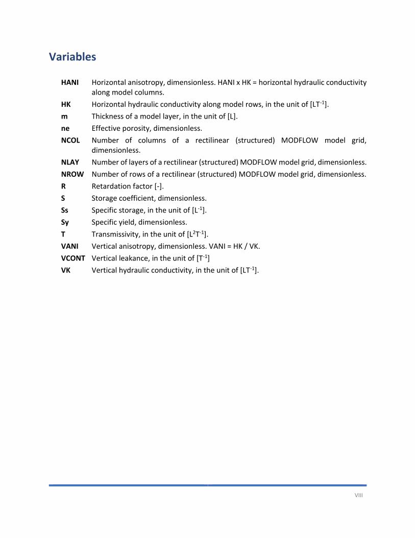
Variables
HANI Horizontal anisotropy, dimensionless. HANI x HK = horizontal hydraulic conductivity along model columns.
HK Horizontal hydraulic conductivity along model rows, in the unit of [LT-1].
m Thickness of a model layer, in the unit of [L].
ne Effective porosity, dimensionless.
NCOL Number of columns of a rectilinear (structured) MODFLOW model grid, dimensionless.
NLAY Number of layers of a rectilinear (structured) MODFLOW model grid, dimensionless.
NROW Number of rows of a rectilinear (structured) MODFLOW model grid, dimensionless.
R Retardation factor [-].
S Storage coefficient, dimensionless.
Ss Specific storage, in the unit of [L-1].
Sy Specific yield, dimensionless.
T Transmissivity, in the unit of [L2T-1].
VANI Vertical anisotropy, dimensionless. VANI = HK / VK.
VCONT Vertical leakance, in the unit of [T-1]
VK Vertical hydraulic conductivity, in the unit of [LT-1].
1 – Introduction 1
Chapter 1. Introduction
1.1. What is Processing Modflow
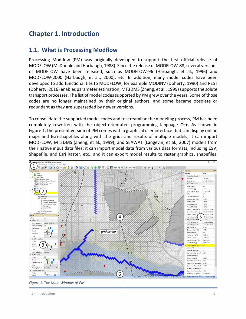
Processing Modflow (PM) was originally developed to support the first official release of MODFLOW (McDonald and Harbaugh, 1988). Since the release of MODFLOW-88, several versions of MODFLOW have been released, such as MODFLOW-96 (Harbaugh, et al., 1996) and MODFLOW-2000 (Harbaugh, et al., 2000), etc. In addition, many model codes have been developed to add functionalities to MODFLOW, for example MODINV (Doherty, 1990) and PEST (Doherty, 2016) enables parameter estimation, MT3DMS (Zheng, et al., 1999) supports the solute transport processes. The list of model codes supported by PM grew over the years. Some of those codes are no longer maintained by their original authors, and some became obsolete or redundant as they are superseded by newer versions. To consolidate the supported model codes and to streamline the modeling process, PM has been completely rewritten with the object-orientated programming language C++. As shown in Figure 1, the present version of PM comes with a graphical user interface that can display online maps and Esri-shapefiles along with the grids and results of multiple models; it can import MODFLOW, MT3DMS (Zheng, et al., 1999), and SEAWAT (Langevin, et al., 2007) models from their native input data files; it can import model data from various data formats, including CSV, Shapefile, and Esri Raster, etc., and it can export model results to raster graphics, shapefiles,
Figure 1. The Main Window of PM
1 – Introduction 2
charts, and/or text files. The list of supported model codes is consolidated to the latest official releases of model codes that are actively maintained at the time of writing, including MODFLOW-2005 (Harbaugh, 2005), SEAWAT (Langevin, et al., 2007), MODFLOW-NWT (Niswonger, et al., 2011), MODPATH (Pollock, 2016), MT3D-USGS (Bedekar, et al., 2016), PEST (Doherty, 2016), BeoPEST (Hunt, et al., 2010), and Zone Budget (Harbaugh, 1990). The support for MODFLOW 6 (Langevin, et al., 2017) will be added in near future. This text focuses on the use of PM and does not attempt to present modeling theories and the conceptualization of various packages. Interested users are referred to the user guides of the supported model codes. In addition to the model documents, many groundwater modeling text books are available at nominal cost. For example, (Anderson, et al., 2015) present a comprehensive reference of applied groundwater modeling and (Doherty, 2015) provides the complete theory of calibration and uncertainty analysis.
1.2. Main Window of PM
The main window of PM and its major features are shown in Figure 1. You may use the mouse to
drag and rearrange the toolbars, the Settings window, and the Properties window. A summary
of these features is given below.
1. Menu Bar and Toolbars:
• The Menu bar contains several menus that are described in detail in Chapter 3 . We use the notation Menu > Item to point to a menu item. For example, File > Save means the menu item “Save” of the “File” menu.
• The File menu is used to save or open PM files, to create or import models, or to save the map in image files. As the Discretization, Parameters, and Models menus only act on the Active model (see TOC below), they are activated only if at least one model is loaded under the Models group of TOC.
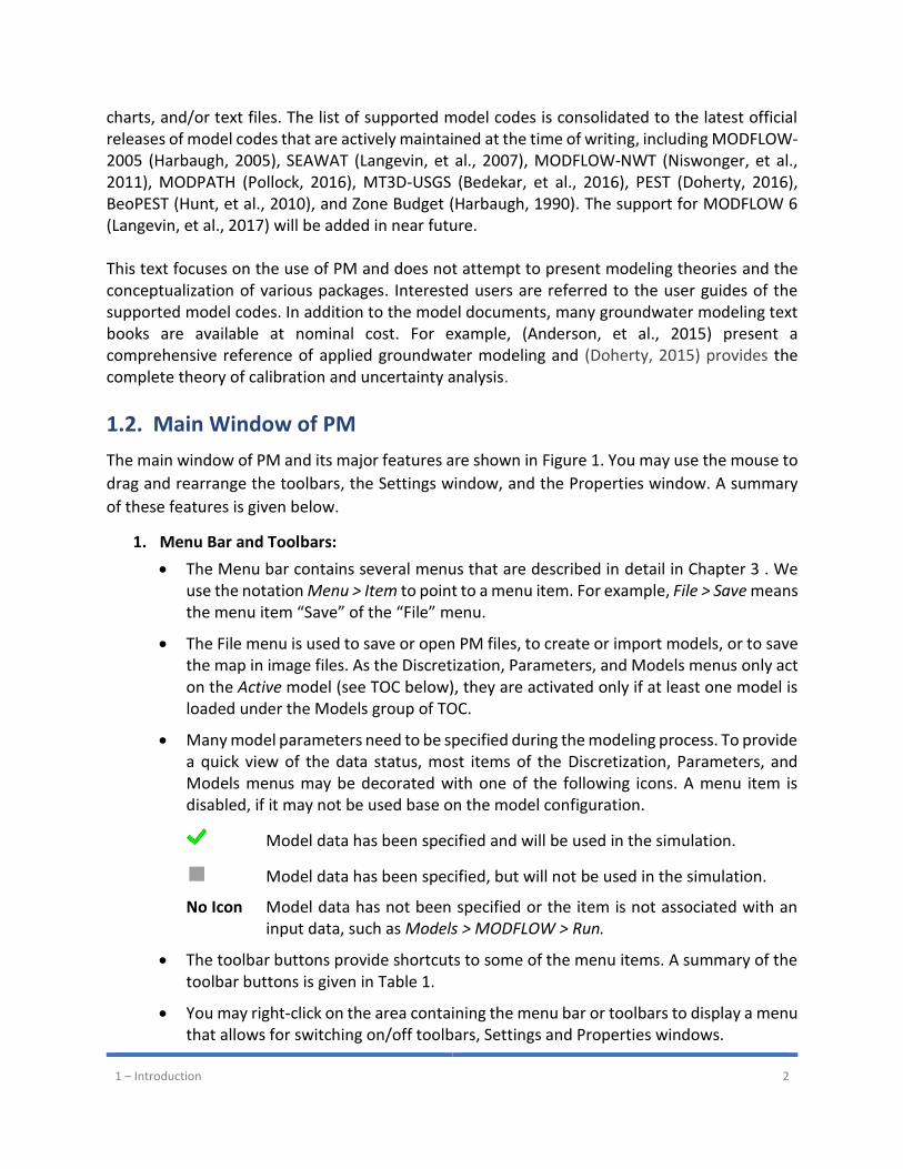
• Many model parameters need to be specified during the modeling process. To provide a quick view of the data status, most items of the Discretization, Parameters, and Models menus may be decorated with one of the following icons. A menu item is disabled, if it may not be used base on the model configuration.
Model data has been specified and will be used in the simulation.
Model data has been specified, but will not be used in the simulation.
No Icon Model data has not been specified or the item is not associated with an input data, such as Models > MODFLOW > Run.
• The toolbar buttons provide shortcuts to some of the menu items. A summary of the toolbar buttons is given in Table 1.
• You may right-click on the area containing the menu bar or toolbars to display a menu that allows for switching on/off toolbars, Settings and Properties windows.

1 – Introduction 3
2. Table of contents Window (TOC) – The TOC contains a list of predefined groups (e.g. Views, Captions, Images, Base Maps, Shapefiles, and Models). Each group contains a list of items (e.g. maps, shapefiles, models, etc.). And, each item represents a map layer that contains a visual representation of the item’s data. When an item is clicked, it is highlighted and becomes the active layer. Only one layer can be the active layer at a time. The Settings and Properties windows (see below) displays the settings and values of the active layer. The major functions of the TOC are briefly described below (see the following chapters for more details).
• Right-click on a group to display a popup menu. This allows the user to add, remove, show, or hide items.
• Right-click on the Models group to create or import models. When multiple models are loaded in the models group, only one model can be set as the Active Model and the Discretization, Parameters, and Models menus only act on the active model. The active model item is highlighted in yellow on the TOC. Right-clicking on a model item to display a pop-up menu with the following menu items:
o Set as Active Model1 – set the model as the active model.
o Zoom to Model – zoom in to the extent of the model.
o Remove Model1 – remove the model and delete its data.
• Right-click on an item to display a popup menu with item-specific functions, such as Zoom To, Remove Package, Export to Shapefile or Export Matrix Data.
• The checkbox in front of a group determines whether its items are displayed or hidden.
• The checkbox in front of an item determines whether it is displayed on the map or hidden. The data of a hidden item remains in the computer’s memory. If an item is no longer needed, its removal is recommended.
3. Settings Window – This window displays the available visualization settings of the active layer. If a setting contains a text string, double-click on the text string to edit it.
4. Map Viewer – This displays base maps, shapefiles, model grid, model cell features, such as wells or stream, and visual representations of model results, such as flow vectors, path lines, head contours, etc.
• The cell that is pointed to by the grid cursor is the active cell.
• You may interact with map with the Pan tool, the Zoom tool, and other tools described in Section 3.5.
• Many map layers have on-map legends that can be turn on by checking the Visible checkbox in the Settings window of the respective map layer. The captions and the contents of the on-map legends are synced with the TOC with the exception that an individual on-map legend can only display up to 40 items. On-map legends can be
1 This option is disabled when the Data Editor (Section 3.3.2) or the Grid Editor (Section 3.3.1) is being used.
1 – Introduction 4
moved or resized with the mouse. Their positions are anchored on the lower-left corner of the Map Viewer and are therefore independent of the zoom level and position of the map contents.
5. Properties Window – This window displays the properties of the selected item of the active layer. For example, if the active layer is a shapefile, this window displays the properties of the selected feature within the shapefile. If the active layer is a model, this window displays the meta data of the model. If a model data, such as Specific Storage, is being edited, this window displays the meta data of the model along with the properties of the cell pointed to by the grid cursor. The cell data that is currently being edited is highlighted in yellow.
6. Status bar – This displays the following information
• The name of the model data set or package that is being edited. For example, Specific Yield or Drain (DRN).
• Current stress period, if the package that is being edited is time-dependent.
• Ground surface elevation at the mouse cursor’s location on the map. Elevation values are provided for reference purposes only and do not represent precisely measured or surveyed values. The ground surface elevation data is provided in the following manner.
o Within most parts of the United States, the elevation data is provided by the Point
Query Service (PQS) based on the National Elevation Dataset (Gesch, et al., 2002)
of the USGS.
o Outside of the United States, the elevation data is provided by Google or
MapQuest web services.
• Coordinates at the mouse cursor’s location on the map. Coordinates are expressed in the World Geodetic System 1984 (National Imagery and Mapping Agency, 1984) datum. For geographic coordinates, negative values are used for longitudinal coordinates in the western hemisphere and latitudinal coordinates in the southern hemisphere. In addition to the geographic coordinates, the Universal Transverse Mercator (Defense Mapping Agency, 1989) coordinates are displayed. The format of the display is “UTM zone Hemisphere: (x, y),” where zone is the zone number of the UTM system ranging from 1 to 60 and Hemisphere is either “N” for North or “S” for South. The coordinates are given as x and y.
• Layer, Row, Column of the active model at the mouse cursor location.
1 – Introduction 5
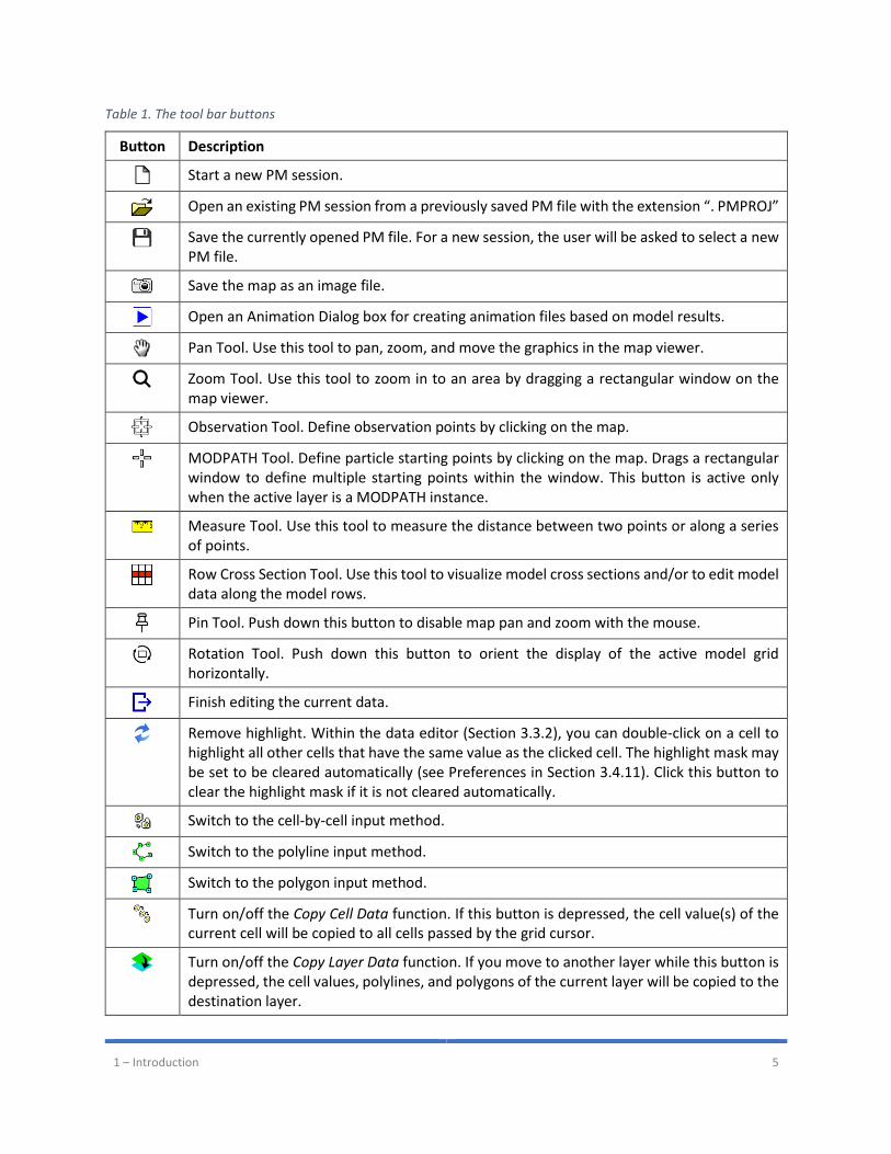
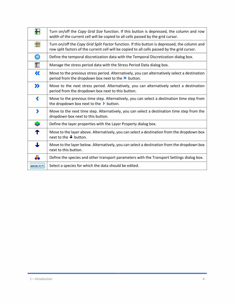
Table 1. The tool bar buttons
Button Description
Start a new PM session.
Open an existing PM session from a previously saved PM file with the extension “. PMPROJ”
Save the currently opened PM file. For a new session, the user will be asked to select a new PM file.
Save the map as an image file.
Open an Animation Dialog box for creating animation files based on model results.
Pan Tool. Use this tool to pan, zoom, and move the graphics in the map viewer.
Zoom Tool. Use this tool to zoom in to an area by dragging a rectangular window on the map viewer.
Observation Tool. Define observation points by clicking on the map.
MODPATH Tool. Define particle starting points by clicking on the map. Drags a rectangular window to define multiple starting points within the window. This button is active only when the active layer is a MODPATH instance.
Measure Tool. Use this tool to measure the distance between two points or along a series of points.
Row Cross Section Tool. Use this tool to visualize model cross sections and/or to edit model data along the model rows.
Pin Tool. Push down this button to disable map pan and zoom with the mouse.
Rotation Tool. Push down this button to orient the display of the active model grid horizontally.
Finish editing the current data.
Remove highlight. Within the data editor (Section 3.3.2), you can double-click on a cell to highlight all other cells that have the same value as the clicked cell. The highlight mask may be set to be cleared automatically (see Preferences in Section 3.4.11). Click this button to clear the highlight mask if it is not cleared automatically.
Switch to the cell-by-cell input method.
Switch to the polyline input method.
Switch to the polygon input method.
Turn on/off the Copy Cell Data function. If this button is depressed, the cell value(s) of the current cell will be copied to all cells passed by the grid cursor.
Turn on/off the Copy Layer Data function. If you move to another layer while this button is depressed, the cell values, polylines, and polygons of the current layer will be copied to the destination layer.
1 – Introduction 6
Turn on/off the Copy Grid Size function. If this button is depressed, the column and row width of the current cell will be copied to all cells passed by the grid cursor.
Turn on/off the Copy Grid Split Factor function. If this button is depressed, the column and row split factors of the current cell will be copied to all cells passed by the grid cursor.
Define the temporal discretization data with the Temporal Discretization dialog box.
Manage the stress period data with the Stress Period Data dialog box.
Move to the previous stress period. Alternatively, you can alternatively select a destination period from the dropdown box next to the button.
Move to the next stress period. Alternatively, you can alternatively select a destination period from the dropdown box next to this button.
Move to the previous time step. Alternatively, you can select a destination time step from the dropdown box next to the button.
Move to the next time step. Alternatively, you can select a destination time step from the dropdown box next to this button.
Define the layer properties with the Layer Property dialog box.
Move to the layer above. Alternatively, you can select a destination from the dropdown box next to the button.
Move to the layer below. Alternatively, you can select a destination from the dropdown box next to this button.
Define the species and other transport parameters with the Transport Settings dialog box.
Select a species for which the data should be edited.
2 – Maps 7
Chapter 2. Maps
2.1. Views
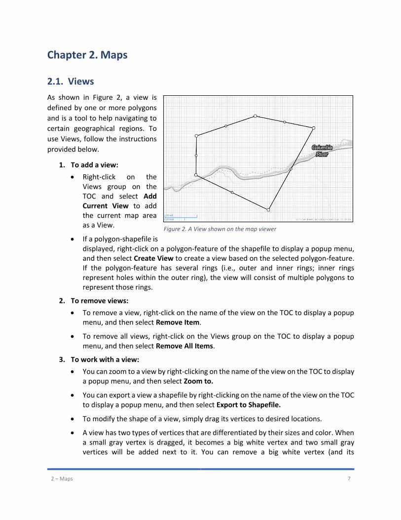
As shown in Figure 2, a view is
defined by one or more polygons
and is a tool to help navigating to
certain geographical regions. To
use Views, follow the instructions
provided below.
1. To add a view:
• Right-click on the Views group on the TOC and select Add Current View to add the current map area as a View.
• If a polygon-shapefile is displayed, right-click on a polygon-feature of the shapefile to display a popup menu, and then select Create View to create a view based on the selected polygon-feature. If the polygon-feature has several rings (i.e., outer and inner rings; inner rings represent holes within the outer ring), the view will consist of multiple polygons to represent those rings.
2. To remove views:
• To remove a view, right-click on the name of the view on the TOC to display a popup menu, and then select Remove Item.
• To remove all views, right-click on the Views group on the TOC to display a popup menu, and then select Remove All Items.
3. To work with a view:
• You can zoom to a view by right-clicking on the name of the view on the TOC to display a popup menu, and then select Zoom to.
• You can export a view a shapefile by right-clicking on the name of the view on the TOC to display a popup menu, and then select Export to Shapefile.
• To modify the shape of a view, simply drag its vertices to desired locations.
• A view has two types of vertices that are differentiated by their sizes and color. When a small gray vertex is dragged, it becomes a big white vertex and two small gray vertices will be added next to it. You can remove a big white vertex (and its
Figure 2. A View shown on the map viewer
2 – Maps 8
neighboring small vertices) by right-clicking on it and then select Remove Vertex from the popup menu.
• If a view contains more than one polygon, you can remove a polygon by right-clicking on one of its vertices and then selecting Remove polygon.
4. To customize the display of a view, click on its name on the TOC, and use its Settings window as described below.
• Name: The text string is the name of the View displayed on the TOC. Double-click the text string to modify.
• Opacity: A view is opaque if the value of opacity is 100, translucent if the value is between 1 and 99, and transparent if the value is 0.
• Polygon Color: Use the dropdown box to define the color of the view.
• Show Vertices: Check/uncheck the box to turn on/off the display of vertices of the view. You may turn off the display of vertices to avoid unintentional modifications.
2.2. Captions
Captions are text strings that can be added to the Map Viewer. A caption is anchored on the
relative position of the map viewer window.
1. To add a caption: Right-click on the Captions group on the TOC and select Add Caption.
2. To remove captions:
• To remove a caption, right-click on the name of the view on the TOC to display a popup menu, and then select Remove Item.
• To remove all captions, right-click on the Views group on the TOC to display a popup menu, and then select Remove All Items.
3. To work with a caption:
• You can move a caption by dragging it with the mouse.
• You can resize a caption by dragging its corners or borders with the mouse.
4. To customize the display of a caption, click on its name on the TOC and use its Settings window as described below.
• Name: The text string is the name of the Caption displayed on the TOC. Double-click the text string to modify.
• Caption Text: This is the text string of the caption. Double-click the text string to modify. If an active model is present, you can insert the following codes to the text string. When you move across time or between layers, these codes will be replaced by the current data of the active model.
o \n = line separator.
o {yyyy} = year. {m} = month. {d} = day.

2 – Maps 9
o {hh} = hour. {mm} = minute. {ss} = second.
o {sm} = short month. {lm} = long month.
o {p} = stress period. {t} = time step. {l} = layer
• Enable Interaction: Check this box to allow moving and resizing the caption with the mouse.
• Opacity: A caption is opaque if the value of opacity is 100, translucent if the value is between 1 and 99, and transparent if the value is 0.
• Color: Use the dropdown box to define the color of the caption.
• Font Family, Font Weight, and Font Style: These define the font for the caption.
• Text Alignment: Use the dropdown box to define the alignment of the text string.
• Text Shadow: Check this box to add shadow to the caption.
2.3. Images
Pixel images or logos can be added as image overlays to the Map Viewer. An image overlay is
anchored on the relative position of the map viewer window.
1. To add an image: Right-click on the Images group on the TOC, select Add Image, and then select an image file from the Open File dialog box.
2. To remove images:
• To remove an image, right-click on the name of the view on the TOC to display a popup menu, and then select Remove Item.
• To remove all images, right-click on the Views group on the TOC to display a popup menu, and then select Remove All Items.
3. To work with an image:
• You can move an image by dragging it with the mouse.
• You can resize an image by dragging its corners or borders with the mouse.
4. To customize the display of an image, use its Settings window as described below.
• Name: The text string is the name of the Image displayed on the TOC. Double-click the text string to modify.
• Enable Interaction: If this box is checked, you can use the mouse to drag and resize the image.
• Opacity: An image is opaque if the value of opacity is 100, translucent if the value is between 1 and 99, and transparent if the value is 0.
2 – Maps 10
2.4. Base Maps
PM can display maps from various tiled-map service providers. Several default map services are
preprogrammed for your convenience, including various OpenStreetMap styles that are
described online at http://wiki.openstreetmap.org/wiki/Tiles. You can add additional tiled-map
services to PM. Always be sure to read the terms of use of a tiled-map service provider and know
its limitations before adding it to PM. The following outlines the procedures for controlling the
display of base maps.
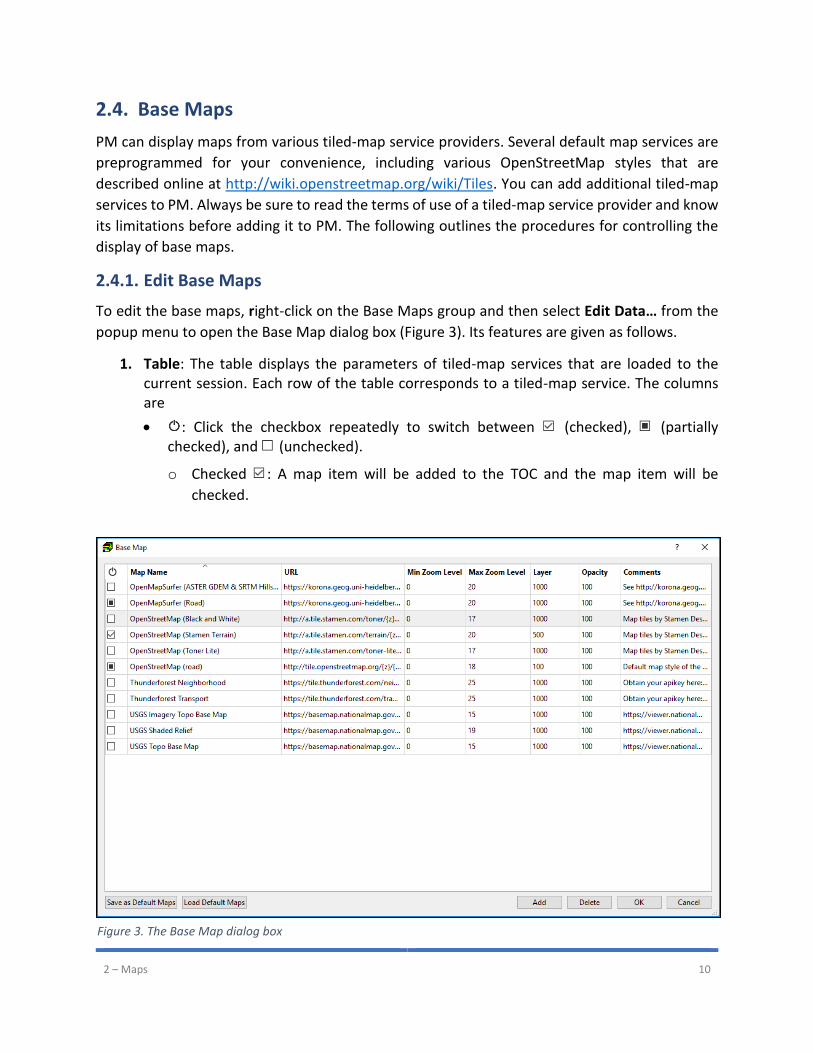
2.4.1. Edit Base Maps
To edit the base maps, right-click on the Base Maps group and then select Edit Data… from the
popup menu to open the Base Map dialog box (Figure 3). Its features are given as follows.
1. Table: The table displays the parameters of tiled-map services that are loaded to the current session. Each row of the table corresponds to a tiled-map service. The columns are
• : Click the checkbox repeatedly to switch between (checked), (partially checked), and (unchecked).
o Checked : A map item will be added to the TOC and the map item will be
checked.
Figure 3. The Base Map dialog box
2 – Maps 11
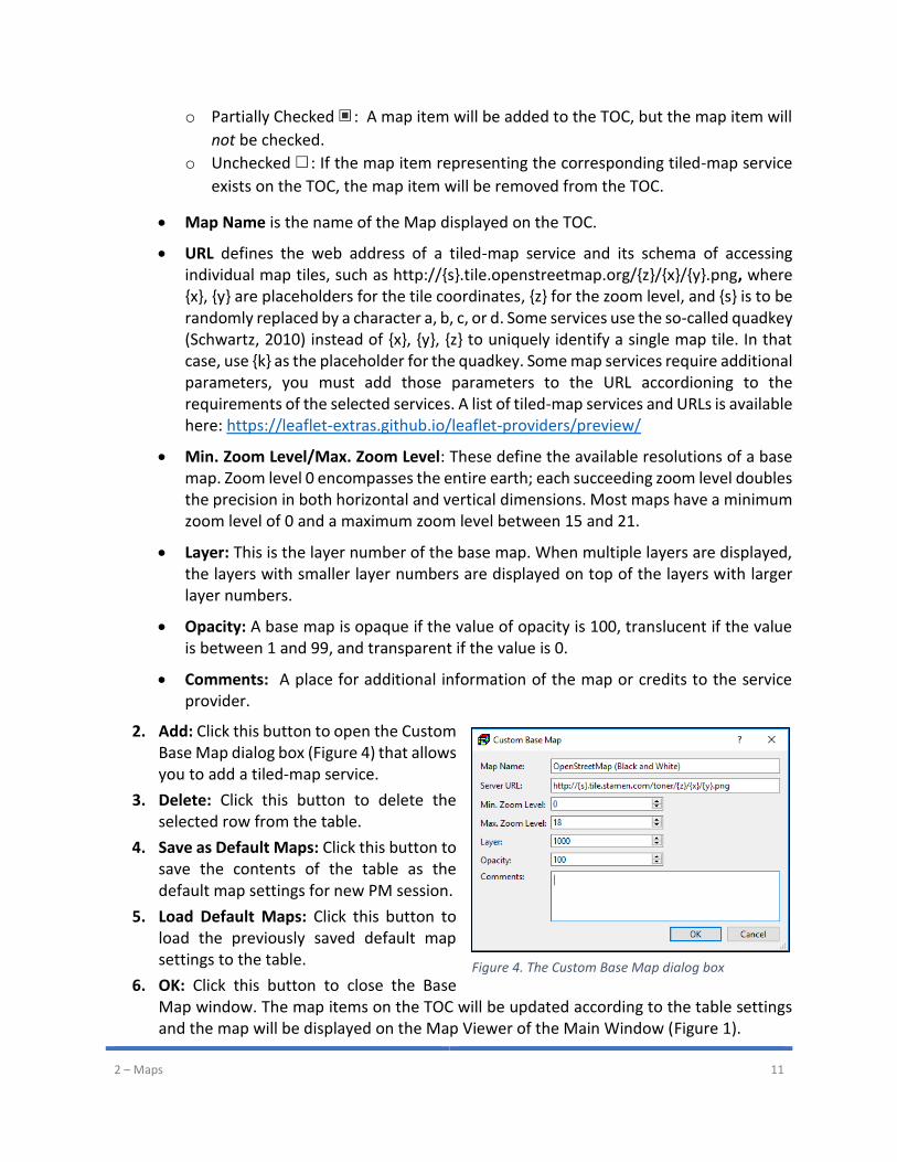
o Partially Checked : A map item will be added to the TOC, but the map item will
not be checked.
o Unchecked : If the map item representing the corresponding tiled-map service
exists on the TOC, the map item will be removed from the TOC.
• Map Name is the name of the Map displayed on the TOC.
• URL defines the web address of a tiled-map service and its schema of accessing individual map tiles, such as http://{s}.tile.openstreetmap.org/{z}/{x}/{y}.png, where {x}, {y} are placeholders for the tile coordinates, {z} for the zoom level, and {s} is to be randomly replaced by a character a, b, c, or d. Some services use the so-called quadkey (Schwartz, 2010) instead of {x}, {y}, {z} to uniquely identify a single map tile. In that case, use {k} as the placeholder for the quadkey. Some map services require additional parameters, you must add those parameters to the URL accordioning to the requirements of the selected services. A list of tiled-map services and URLs is available here: https://leaflet-extras.github.io/leaflet-providers/preview/
• Min. Zoom Level/Max. Zoom Level: These define the available resolutions of a base map. Zoom level 0 encompasses the entire earth; each succeeding zoom level doubles the precision in both horizontal and vertical dimensions. Most maps have a minimum zoom level of 0 and a maximum zoom level between 15 and 21.
• Layer: This is the layer number of the base map. When multiple layers are displayed, the layers with smaller layer numbers are displayed on top of the layers with larger layer numbers.
• Opacity: A base map is opaque if the value of opacity is 100, translucent if the value is between 1 and 99, and transparent if the value is 0.
• Comments: A place for additional information of the map or credits to the service provider.
2. Add: Click this button to open the Custom Base Map dialog box (Figure 4) that allows you to add a tiled-map service.
3. Delete: Click this button to delete the selected row from the table.
4. Save as Default Maps: Click this button to save the contents of the table as the default map settings for new PM session.
5. Load Default Maps: Click this button to load the previously saved default map settings to the table.
6. OK: Click this button to close the Base Map window. The map items on the TOC will be updated according to the table settings and the map will be displayed on the Map Viewer of the Main Window (Figure 1).
Figure 4. The Custom Base Map dialog box
2 – Maps 12
2.4.2. Customize the Display of a Base Map
When selected as the active layer, a base map can be modified in its Settings window. The fields
in the Settings window are listed below.
1. General group
• Name: The text string is the name of the Map displayed on the TOC. Double-click the text string to modify.
• Opacity: A base map is opaque if the value of opacity is 100, translucent if the value is between 1 and 99, and transparent if the value is 0.
• Layer: This is the layer number of the base map. When multiple layers are displayed, the layers with smaller layer numbers are displayed on top of the layers with larger layer numbers.
• Min./Max. Zoom Level: These define the available resolutions of a base map. Zoom level 0 encompasses the entire earth; each succeeding zoom level doubles the precision in both horizontal and vertical dimensions. Most maps have a minimum zoom level of 0 and a maximum zoom level between 15 and 21.
2.5. Shapefiles
The shapefile2 format (ESRI, 1998) is a geospatial vector format describing spatial features such
as points, polylines, and polygons. Each spatial feature is associated with attributes, such as name
or temperature. The shapefile format consists of a collection of files with a common base
filename, stored in the same directory. Shapefiles may be displayed on the Map Viewer for
referencing purposes. Attributes of shapefile polygon features may be imported to model cells
directly (See Section 3.5 for details).
When using a shapefile within PM, the files with the following extensions are mandatory:
1. .shp – contains the geometry of spatial features.
2. .dbf – contains the attributes of each spatial features.
3. .prj – contains the coordinate system and projection information.
4. .shx – contains index of the spatial features. It allows fast forward and backward seeking by some software applications. PM does not use this file, but will create it when exporting a shapefile.
2.5.1. Add Shapefiles to the Map Viewer
1. Right-click on the Shapefile group on the TOC, and then select Add from the popup menu to display the Open File dialog box.
2 Follow these links SURFER or AutoCAD for details about exporting to shapefile from the respective software.
2 – Maps 13
2. In the Open File dialog box, select the desired shapefile and then click Open to add the selected shapefile to the Map Viewer. Note that the added shapefiles are compressed and then embedded in the saved PM (.pmproj) files. This allows you to share .pmproj files with other users without having to send out shapefiles separately.
2.5.2. Customize the Display of a Shapefile
By default, a shapefile is displayed in a single color. To customize the display of a shapefile, use
its Settings window and Symbology dialog box as described below.
2.5.2.1. The Settings Window
The following options are available in the Settings window of a shapefile.
1. General Group
• Name: The text string is the name of the Shapefile displayed on the TOC and is used as the caption of the on-map legend (see below). Double-click the text string to modify.
• Identify By: Select a field to be used to identify similar features of a shapefile. When a feature of a shapefile file is clicked, all features of the shapefile with the same value in the selected field are highlighted.
• Opacity: A shapefile is opaque if the value of opacity is 100, translucent if the value is between 1 and 99, and transparent if the value is 0.
• Layer: This is the layer number of the aerial photograph. When multiple layers are displayed in HDX, the layers with smaller layer numbers are displayed on top of the map layers with larger layer numbers.
• Line Weight: This defines the width of displayed line segments in pixels.
• Colors: This displays the color(s) that are currently in use. The colors can be defined using the Symbology dialog box. To open the Symbology dialog box, click on the button (The Symbology dialog box is discussed in the following section.)
• Pickable: Check this box to make the shapefile pickable. When a shapefile is pickable, its features may be picked by mouse clicks.
2. On-map Legend Group
• Visible: Check this box to display the on-map legend.
• Enable Interaction: If this box is checked, you can use the mouse to drag and resize the on-map legend.
• Opacity: The legend is opaque if the value of opacity is 100, translucent if the value is between 1 and 99, and transparent if the value is 0.
• Width: This defines the relative width of the legend. The larger the number the wider is the legend.
2 – Maps 14
• Reset Legend: Click the Reset button to reset the legend to its default size and position.
3. Label Group
• Visible: Check this box to display labels.
• Field: This dropdown box contains the attribute fields for the selected shapefile. Use this box to select the field used for labeling displayed shapes.
• Display Label: This dropdown box controls when the labels should be displayed.
• Size: This defines the font size of the labels.
• Color: This defines the color of the labels.
4. Point Feature Group: The definitions of this group are ignored if point features are not present in the shapefile.
• Type: This dropdown box defines the shape of point features.
• Size: This dropdown box defines the appearance size of the point features.
5. Polyline Feature Group: The definitions of this group are ignored if polyline features are not present in the shapefile.
• Label Distance: This dropdown box adjusts the distance between labels along displayed polylines.
6. Polygon Feature: The definitions of this group are ignored if polygon features are not present in the shapefile.
• Fill Polygon: If this box is checked, all polygon features of the loaded shapefile will be filled with the color(s) defined in the Symbology dialog box (see below).
2.5.2.2. The Symbology Dialog Box
Spatial features of a shapefile are associated attribute values. The Symbology dialog box can be
used to modify how these values are presented with the spatial features. To open this dialog box,
click on the button in the Colors field in the Settings window of the shapefile. Three color-
mapping styles are available and can be selected using the Style dropdown box:
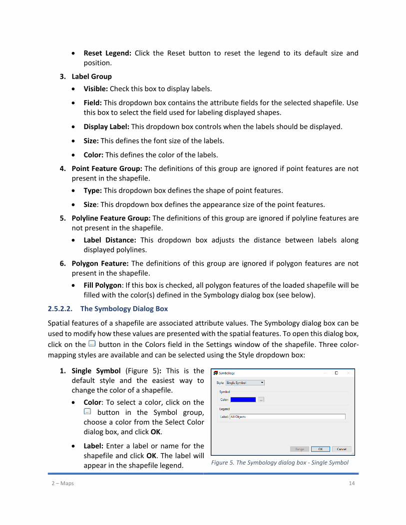
1. Single Symbol (Figure 5): This is the default style and the easiest way to change the color of a shapefile.
• Color: To select a color, click on the
button in the Symbol group, choose a color from the Select Color dialog box, and click OK.
• Label: Enter a label or name for the shapefile and click OK. The label will appear in the shapefile legend. Figure 5. The Symbology dialog box - Single Symbol

2 – Maps 15
2. Unique Values (Figure 6): PM can assign a color to each unique value within a selected value field. For example, if a shapefile were to have a value field for land use, a different color could be selected to represent each type of land use (i.e. residential, commercial, agricultural, etc.).
• Fields: This dropdown box contains the value fields for the selected shapefile. Use this box to select a value field.
• Color Scheme: This dropdown box contains several pre-defined color schemes. Use this box to select a color scheme.
• Symbol: This column displays the colors generated from the selected color scheme. To change a color, double-click on it and choose a new color from the Select Color dialog box.
• Value: This column displays the unique values (or strings) of the selected value field. Values cannot be modified.
3. Graduated Colors (Figure 7): In this style, the quantitative values of a value field are grouped into classes, and each class is identified by a color. A choropleth map can also be displayed by mapping quantitative values, such as concentration, to a color ramp. For example, darker shades of red could be used to represent higher concentration values and lighter shades could be used to represent lower concentration values. The following describes the options available with the Graduated Colors style:
• Fields Group: Use the Value dropdown box to select the field that contains the desired quantitative values. Use the Normalization dropdown box to select a field to normalize the data of the Value field. HydroDaVE divides the data of the Value field by the data of the Normalization field and maps the results.
• Classification Group: Use the Classes dropdown box to define the desired number of classes to be displayed. Use the Color Ramp dropdown box to assign graduated colors to the classes.
Figure 6. The Symbology dialog box - Unique Values
Figure 7. The Symbology dialog box - Graduated Colors

2 – Maps 16
• Range: Click this button to specify the lower and upper bounds of the quantitative values to be mapped. The defined range is divided into equal-interval sub-ranges for each class.
• Symbol: This column displays the colors of the individual classes. Colors are defined by the selected color ramp. To change a particular color, double-click on the displayed color box and choose a new color from the Select Color dialog box.
• Value: This column displays the lower and upper bounds of the individual classes. Values cannot be modified.
3 – Modeling Environment 17
Chapter 3. Modeling Environment
3.1. Units
PM requires the use of consistent units throughout the modeling process. For example, if you are
using length [L] units of meters and time [T] units of seconds, hydraulic conductivity will be
expressed in units of [m/s], pumping rates will be in units of [m3/s] and dispersivity will be in units
of [m]. The values of the simulation results are also expressed in the same units. Inconsistent
units can be specified for concentration units (for example, mg/L in model with length units of
m), as long as the user recognizes that the masses will be reported in unconventional units (in
this case [m3 · mg/L]).
Independent of your language and regional settings, PM always uses period (.) as the decimal
point for decimal numerals.
3.2. Temporal Discretization
MODFLOW divides the simulation time into stress periods, which are, in turn, divided into time
steps. The model input parameters are assumed to be constant during a given stress period. For
transient flow simulations involving multiple stress periods, the user has the option of changing
parameters associated with most flow packages, such as River or Well, from a stress period to
another. For transport simulations, the user may change mass-loading rates and source
concentrations associated with the fluid sources and sinks.
The numbers of stress periods and time steps as well as the length of the simulation are defined
when creating a new model (Section 3.4.6) or importing an existing model (Section 3.4.7). These
values can be modified with the Time dialog box. See Section 3.6.1 for details.
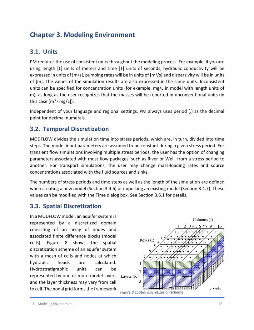
3.3. Spatial Discretization
In a MODFLOW model, an aquifer system is
represented by a discretized domain
consisting of an array of nodes and
associated finite difference blocks (model
cells). Figure 8 shows the spatial
discretization scheme of an aquifer system
with a mesh of cells and nodes at which
hydraulic heads are calculated.
Hydrostratigraphic units can be
represented by one or more model layers
and the layer thickness may vary from cell
to cell. The nodal grid forms the framework Figure 8 Spatial discretization scheme

3 – Modeling Environment 18
of the finite-difference numerical model. Once the head values are computed, they are used to
calculate the cell-by-cell flow terms. The calculated head values and flow terms are the basis for
water budget calculation, particle tracking, transport models, and visualization, such as flow
vectors and contours.
PM uses the index notation [Layer, Row, Column] to describe the location of a cell in a 3D array.
For example, the cell located in the first layer, 6th row, and 2nd column is denoted by [1, 6, 2].
For 2D arrays, the index notation [Row, Column] is used.
The numbers of layers, columns, and rows as well as column and row widths are defined when
creating a new model (Section 3.4.6) or importing an existing model (Section 3.4.7). These values
can be modified with the Grid Editor. See Section 3.3.1 for details.
Model parameters (such as hydraulic conductivity or initial head) and features (such as well or
river) are assigned to individual cells with the Data Editor. See Section 3.3.2 for details.
3.3.1. Grid Editor
1. To start the Grid Editor, select Discretization > Grid. Figure 9 shows the Grid Editor with the grid cursor highlights the entire row and column at the cell location. You may use the Pan tool (Section 3.5.1) and Zoom tool (Section 3.5.2) to interact with the map, to move the grid cursor and/or the model grid.
Figure 9. The Grid Editor with the grid cursor
3 – Modeling Environment 19
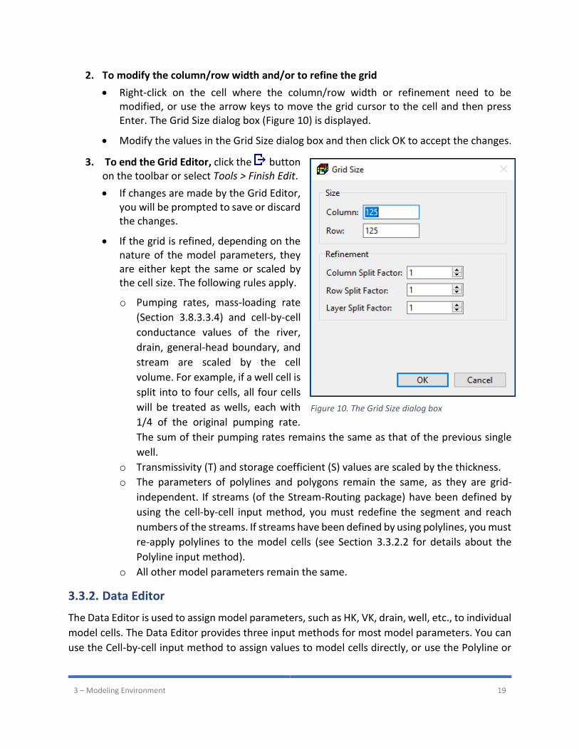
2. To modify the column/row width and/or to refine the grid
• Right-click on the cell where the column/row width or refinement need to be modified, or use the arrow keys to move the grid cursor to the cell and then press Enter. The Grid Size dialog box (Figure 10) is displayed.
• Modify the values in the Grid Size dialog box and then click OK to accept the changes.
3. To end the Grid Editor, click the button on the toolbar or select Tools > Finish Edit.
• If changes are made by the Grid Editor, you will be prompted to save or discard the changes.
• If the grid is refined, depending on the nature of the model parameters, they are either kept the same or scaled by the cell size. The following rules apply.
o Pumping rates, mass-loading rate
(Section 3.8.3.3.4) and cell-by-cell
conductance values of the river,
drain, general-head boundary, and
stream are scaled by the cell
volume. For example, if a well cell is
split into to four cells, all four cells
will be treated as wells, each with
1/4 of the original pumping rate.
The sum of their pumping rates remains the same as that of the previous single
well.
o Transmissivity (T) and storage coefficient (S) values are scaled by the thickness.
o The parameters of polylines and polygons remain the same, as they are grid-
independent. If streams (of the Stream-Routing package) have been defined by
using the cell-by-cell input method, you must redefine the segment and reach
numbers of the streams. If streams have been defined by using polylines, you must
re-apply polylines to the model cells (see Section 3.3.2.2 for details about the
Polyline input method).
o All other model parameters remain the same.
3.3.2. Data Editor
The Data Editor is used to assign model parameters, such as HK, VK, drain, well, etc., to individual
model cells. The Data Editor provides three input methods for most model parameters. You can
use the Cell-by-cell input method to assign values to model cells directly, or use the Polyline or
Figure 10. The Grid Size dialog box
3 – Modeling Environment 20
Polygon input methods to help assigning model parameter to model cells. Regardless of the input
methods being used, PM always use the cell-by-cell model parameters in the simulation.
1. To start the Data Editor, select a menu item from the Discretization, Parameters, or Models menu.
2. To end the Data Editor, click the button on the toolbar or select Tools > Finish Edit.
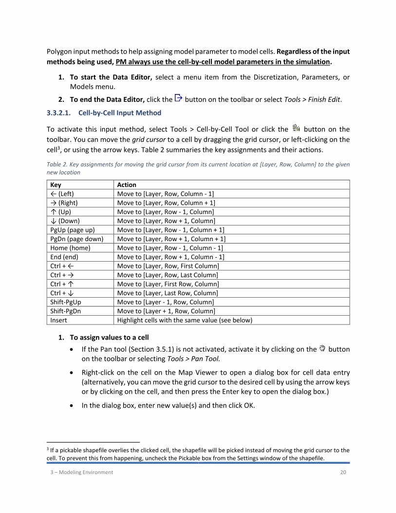
3.3.2.1. Cell-by-Cell Input Method
To activate this input method, select Tools > Cell-by-Cell Tool or click the button on the
toolbar. You can move the grid cursor to a cell by dragging the grid cursor, or left-clicking on the
cell3, or using the arrow keys. Table 2 summaries the key assignments and their actions.
Table 2. Key assignments for moving the grid cursor from its current location at [Layer, Row, Column] to the given new location
Key Action
← (Left) Move to [Layer, Row, Column - 1]
→ (Right) Move to [Layer, Row, Column + 1]
↑ (Up) Move to [Layer, Row - 1, Column]
↓ (Down) Move to [Layer, Row + 1, Column]
PgUp (page up) Move to [Layer, Row - 1, Column + 1]
PgDn (page down) Move to [Layer, Row + 1, Column + 1]
Home (home) Move to [Layer, Row - 1, Column - 1]
End (end) Move to [Layer, Row + 1, Column - 1]
Ctrl + ← Move to [Layer, Row, First Column]
Ctrl + → Move to [Layer, Row, Last Column]
Ctrl + ↑ Move to [Layer, First Row, Column]
Ctrl + ↓ Move to [Layer, Last Row, Column]
Shift-PgUp Move to [Layer - 1, Row, Column]
Shift-PgDn Move to [Layer + 1, Row, Column]
Insert Highlight cells with the same value (see below)
1. To assign values to a cell
• If the Pan tool (Section 3.5.1) is not activated, activate it by clicking on the button on the toolbar or selecting Tools > Pan Tool.
• Right-click on the cell on the Map Viewer to open a dialog box for cell data entry (alternatively, you can move the grid cursor to the desired cell by using the arrow keys or by clicking on the cell, and then press the Enter key to open the dialog box.)
• In the dialog box, enter new value(s) and then click OK.
3 If a pickable shapefile overlies the clicked cell, the shapefile will be picked instead of moving the grid cursor to the cell. To prevent this from happening, uncheck the Pickable box from the Settings window of the shapefile.
3 – Modeling Environment 21
• Some packages4 allows you to assign multiple instances of package-specific features to a cell. For example, you may assign multiple wells to a cell in the Well Package. In that case, the dialog box will include the following functions:
o More Actions > Add: Add a new instance to the current cell.
o More Actions > Delete: Delete current instance from the current cell.
o More Actions > Delete All: Delete all instances from the current cell.
o : go to previous or next instance of the current cell.
2. To highlight cells with the same value
• Within the Data Editor, you can double-click on a cell (or press the Insert key) to highlight all other cells that have the same cell value as the clicked cell. The number of highlighted cells will be briefly displayed on the status bar.
• When you are editing the data of a package, you can select a Highlight Parameter from the package’s Settings window. The values of the selected Highlight Parameter will be used for highlighting.
• The highlight color changes with repeated double-clicks.
• The highlight opacity may be modified by adjusting the value of Highlight Opacity in the Preferences dialog box.
3. To reset, modify, import, and export the values of the current layer or the entire model, see the Data menu (Section 3.5.17) for details.
3.3.2.2. Polyline Input Method5
To activate this input method, select Tools > Polyline Tool or click the button on the toolbar.
The use of this input method is straightforward. First, you create polylines on the Map Viewer,
assign data to vertices of the polylines, and then apply the vertex data to cells along the polylines
by means of linear interpolation.
1. To create/edit polylines
• If the Pan tool (Section 3.5.1) is not activated, activate it by clicking on the button on the toolbar or selecting Tools > Pan Tool.
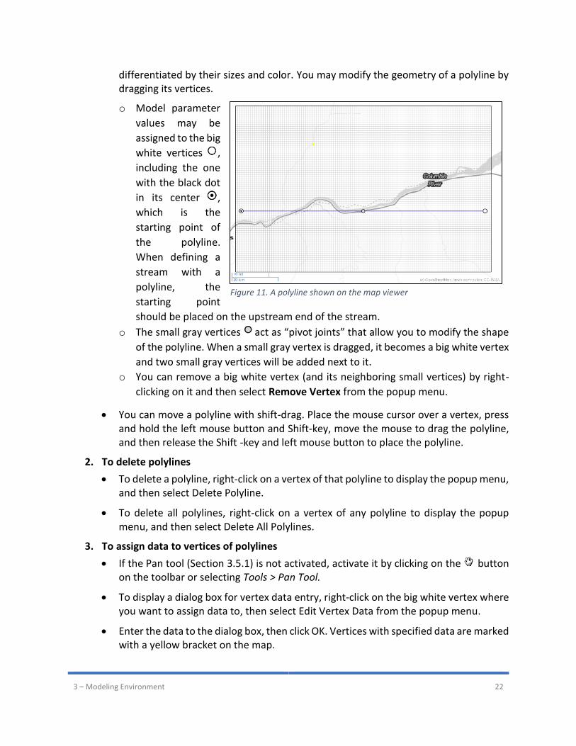
• Right-click on the Map Viewer and then select Add Polyline from the popup menu. A polyline will be added to the map (Figure 11). The polyline is centered on the clicked location and stretched to east and west bounds of the current view. The polyline is associated with the current model layer and has three types of vertices that are
4 The following packages allow for assigning multiple instances of package-specific features to a cell: CHD, DRN, DRT1, FHB1, GHB, HFB6, MNW1, RIV, STR, and WEL. 5 The Polyline input method does not support all model parameters/packages. If a model parameter/package is not
supported, this method and the button are deactivated.
3 – Modeling Environment 22
differentiated by their sizes and color. You may modify the geometry of a polyline by dragging its vertices.
o Model parameter
values may be
assigned to the big
white vertices ,
including the one
with the black dot
in its center ,
which is the
starting point of
the polyline.
When defining a
stream with a
polyline, the
starting point
should be placed on the upstream end of the stream.
o The small gray vertices act as “pivot joints” that allow you to modify the shape
of the polyline. When a small gray vertex is dragged, it becomes a big white vertex
and two small gray vertices will be added next to it.
o You can remove a big white vertex (and its neighboring small vertices) by right-
clicking on it and then select Remove Vertex from the popup menu.
• You can move a polyline with shift-drag. Place the mouse cursor over a vertex, press and hold the left mouse button and Shift-key, move the mouse to drag the polyline, and then release the Shift -key and left mouse button to place the polyline.
2. To delete polylines
• To delete a polyline, right-click on a vertex of that polyline to display the popup menu, and then select Delete Polyline.
• To delete all polylines, right-click on a vertex of any polyline to display the popup menu, and then select Delete All Polylines.
3. To assign data to vertices of polylines
• If the Pan tool (Section 3.5.1) is not activated, activate it by clicking on the button on the toolbar or selecting Tools > Pan Tool.
• To display a dialog box for vertex data entry, right-click on the big white vertex where you want to assign data to, then select Edit Vertex Data from the popup menu.
• Enter the data to the dialog box, then click OK. Vertices with specified data are marked with a yellow bracket on the map.
Figure 11. A polyline shown on the map viewer
3 – Modeling Environment 23
• To clear the specified data of a vertex, right-click on that vertex, and then select Clear Vertex Data from the popup menu.
4. To apply the vertex data to model cells along polylines
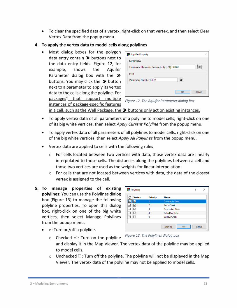
• Most dialog boxes for the polygon
data entry contain buttons next to the data entry fields. Figure 12, for example, shows the Aquifer
Parameter dialog box with the
buttons. You may click the button next to a parameter to apply its vertex data to the cells along the polyline. For packages4 that support multiple instances of package-specific features
in a cell, such as the Well Package, the buttons only act on existing instances.
• To apply vertex data of all parameters of a polyline to model cells, right-click on one of its big white vertices, then select Apply Current Polyline from the popup menu.
• To apply vertex data of all parameters of all polylines to model cells, right-click on one of the big white vertices, then select Apply All Polylines from the popup menu.
• Vertex data are applied to cells with the following rules
o For cells located between two vertices with data, those vertex data are linearly
interpolated to those cells. The distances along the polylines between a cell and
those two vertices are used as the weights for linear interpolation.
o For cells that are not located between vertices with data, the data of the closest
vertex is assigned to the cell.
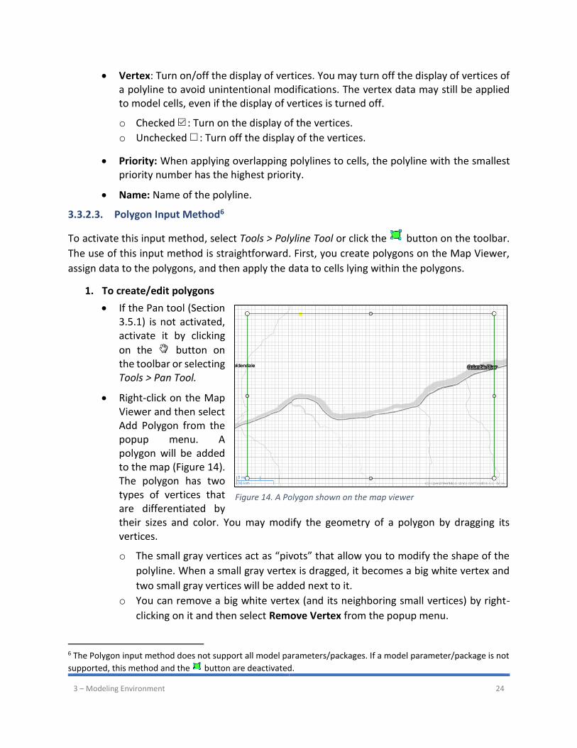
5. To manage properties of existing polylines: You can use the Polylines dialog box (Figure 13) to manage the following polyline properties. To open this dialog box, right-click on one of the big white vertices, then select Manage Polylines from the popup menu.
• : Turn on/off a polyline.
o Checked : Turn on the polyline
and display it in the Map Viewer. The vertex data of the polyline may be applied
to model cells.
o Unchecked : Turn off the polyline. The polyline will not be displayed in the Map
Viewer. The vertex data of the polyline may not be applied to model cells.
Figure 12. The Aquifer Parameter dialog box
Figure 13. The Polylines dialog box
3 – Modeling Environment 24
• Vertex: Turn on/off the display of vertices. You may turn off the display of vertices of a polyline to avoid unintentional modifications. The vertex data may still be applied to model cells, even if the display of vertices is turned off.
o Checked : Turn on the display of the vertices.
o Unchecked : Turn off the display of the vertices.
• Priority: When applying overlapping polylines to cells, the polyline with the smallest priority number has the highest priority.
• Name: Name of the polyline.
3.3.2.3. Polygon Input Method6
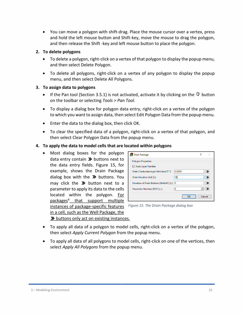
To activate this input method, select Tools > Polyline Tool or click the button on the toolbar.
The use of this input method is straightforward. First, you create polygons on the Map Viewer,
assign data to the polygons, and then apply the data to cells lying within the polygons.
1. To create/edit polygons
• If the Pan tool (Section 3.5.1) is not activated, activate it by clicking
on the button on the toolbar or selecting Tools > Pan Tool.
• Right-click on the Map Viewer and then select Add Polygon from the popup menu. A polygon will be added to the map (Figure 14). The polygon has two types of vertices that are differentiated by their sizes and color. You may modify the geometry of a polygon by dragging its vertices.
o The small gray vertices act as “pivots” that allow you to modify the shape of the
polyline. When a small gray vertex is dragged, it becomes a big white vertex and
two small gray vertices will be added next to it.
o You can remove a big white vertex (and its neighboring small vertices) by right-
clicking on it and then select Remove Vertex from the popup menu.
6 The Polygon input method does not support all model parameters/packages. If a model parameter/package is not
supported, this method and the button are deactivated.
Figure 14. A Polygon shown on the map viewer
3 – Modeling Environment 25
• You can move a polygon with shift-drag. Place the mouse cursor over a vertex, press and hold the left mouse button and Shift-key, move the mouse to drag the polygon, and then release the Shift -key and left mouse button to place the polygon.
2. To delete polygons
• To delete a polygon, right-click on a vertex of that polygon to display the popup menu, and then select Delete Polygon.
• To delete all polygons, right-click on a vertex of any polygon to display the popup menu, and then select Delete All Polygons.
3. To assign data to polygons
• If the Pan tool (Section 3.5.1) is not activated, activate it by clicking on the button on the toolbar or selecting Tools > Pan Tool.
• To display a dialog box for polygon data entry, right-click on a vertex of the polygon to which you want to assign data, then select Edit Polygon Data from the popup menu.
• Enter the data to the dialog box, then click OK.
• To clear the specified data of a polygon, right-click on a vertex of that polygon, and then select Clear Polygon Data from the popup menu.
4. To apply the data to model cells that are located within polygons
• Most dialog boxes for the polygon
data entry contain buttons next to the data entry fields. Figure 15, for example, shows the Drain Package
dialog box with the buttons. You
may click the button next to a parameter to apply its data to the cells located within the polygon. For packages4 that support multiple instances of package-specific features in a cell, such as the Well Package, the
buttons only act on existing instances.
• To apply all data of a polygon to model cells, right-click on a vertex of the polygon, then select Apply Current Polygon from the popup menu.
• To apply all data of all polygons to model cells, right-click on one of the vertices, then select Apply All Polygons from the popup menu.
Figure 15. The Drain Package dialog box
3 – Modeling Environment 26
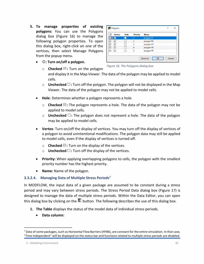
5. To manage properties of existing polygons: You can use the Polygons dialog box (Figure 16) to manage the following polygon properties. To open this dialog box, right-click on one of the vertices, then select Manage Polygons from the popup menu.
• : Turn on/off a polygon.
o Checked : Turn on the polygon
and display it in the Map Viewer. The data of the polygon may be applied to model
cells.
o Unchecked : Turn off the polygon. The polygon will not be displayed in the Map
Viewer. The data of the polygon may not be applied to model cells.
• Hole: Determines whether a polygon represents a hole.
o Checked : The polygon represents a hole. The data of the polygon may not be
applied to model cells.
o Unchecked : The polygon does not represent a hole. The data of the polygon
may be applied to model cells.
• Vertex: Turn on/off the display of vertices. You may turn off the display of vertices of a polygon to avoid unintentional modifications. The polygon data may still be applied to model cells, even if the display of vertices is turned off.
o Checked : Turn on the display of the vertices.
o Unchecked : Turn off the display of the vertices.
• Priority: When applying overlapping polygons to cells, the polygon with the smallest priority number has the highest priority.
• Name: Name of the polygon.
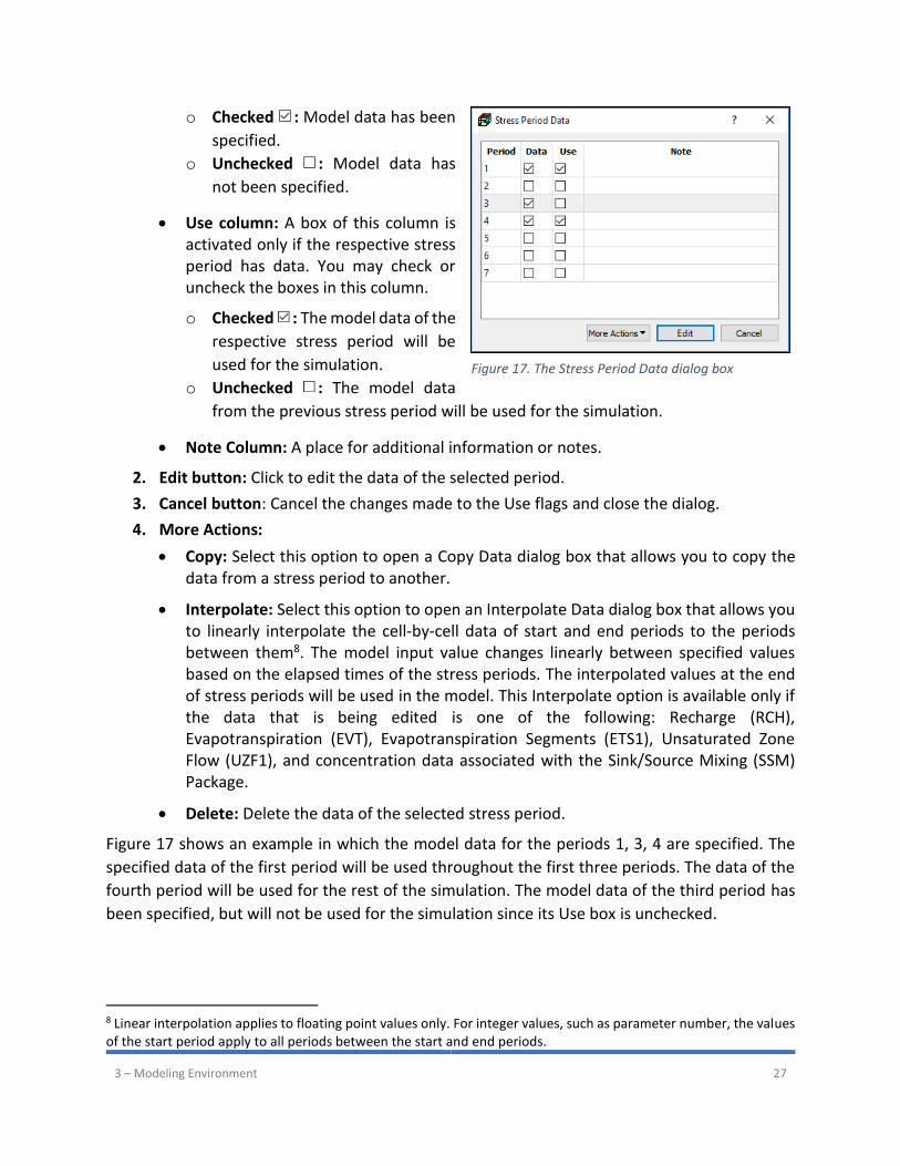
3.3.2.4. Managing Data of Multiple Stress Periods7
In MODFLOW, the input data of a given package are assumed to be constant during a stress
period and may vary between stress periods. The Stress Period Data dialog box (Figure 17) is
designed to manage the data of multiple stress periods. Within the Data Editor, you can open
this dialog box by clicking on the button. The following describes the use of this dialog box.
1. The Table displays the status of the model data of individual stress periods.
• Data column:
7 Data of some packages, such as Horizontal Flow Barriers (HFB6), are constant for the entire simulation. In that case, “Time Independent” will be displayed on the status bar and functions related to multiple stress periods are disabled.
Figure 16. The Polygons dialog box
3 – Modeling Environment 27
o Checked : Model data has been
specified.
o Unchecked : Model data has
not been specified.
• Use column: A box of this column is activated only if the respective stress period has data. You may check or uncheck the boxes in this column.
o Checked : The model data of the
respective stress period will be
used for the simulation.
o Unchecked : The model data
from the previous stress period will be used for the simulation.
• Note Column: A place for additional information or notes.
2. Edit button: Click to edit the data of the selected period.
3. Cancel button: Cancel the changes made to the Use flags and close the dialog.
4. More Actions:
• Copy: Select this option to open a Copy Data dialog box that allows you to copy the data from a stress period to another.
• Interpolate: Select this option to open an Interpolate Data dialog box that allows you to linearly interpolate the cell-by-cell data of start and end periods to the periods between them8. The model input value changes linearly between specified values based on the elapsed times of the stress periods. The interpolated values at the end of stress periods will be used in the model. This Interpolate option is available only if the data that is being edited is one of the following: Recharge (RCH), Evapotranspiration (EVT), Evapotranspiration Segments (ETS1), Unsaturated Zone Flow (UZF1), and concentration data associated with the Sink/Source Mixing (SSM) Package.
• Delete: Delete the data of the selected stress period.
Figure 17 shows an example in which the model data for the periods 1, 3, 4 are specified. The
specified data of the first period will be used throughout the first three periods. The data of the
fourth period will be used for the rest of the simulation. The model data of the third period has
been specified, but will not be used for the simulation since its Use box is unchecked.
8 Linear interpolation applies to floating point values only. For integer values, such as parameter number, the values of the start period apply to all periods between the start and end periods.
Figure 17. The Stress Period Data dialog box

3 – Modeling Environment 28
3.4. File Menu
3.4.1. New
Starts a new PM session. If changes have been made to the current session, you will be prompted
to save the changes to a PM file with the file extension “.pmproj”. A PM file contains model data
and settings of all graphical objects, except for the model results and online base maps. Links to
the model results are stored in the PM file.
3.4.2. Open
Opens an existing PM file9 in the Open Processing Modflow File dialog box. If changes have been
made to the current session, you will be prompted to save the changes to a PM file with the file
extension “.pmproj”. A PM file contains model data and settings of all graphical objects, except
for the model results and online base maps. Links to the model results are stored in the PM file.
3.4.3. Recent Files
Allows you to open a PM file from the list of recently accessed files.
3.4.4. Save
Saves the model data and settings to the currently opened PM file. For a new PM session, you
will be asked to select a new PM file from the Save As dialog box.
A backup of the original PM file is created, before it is saved. The filename of a backup file consists
of the original filename and the string “.~bak~YYYYMMDDHHMMSS”, where YYYY is year, MM is
month, DD is day, HH is hour, MM is minute, and SS is second at which the backup file is created.
The maximum number of backups is defined in the Preferences dialog box (Section 3.4.11). To
restore a backup file, just rename it by removing the string “.~bak~YYYYMMDDHHMMSS”.
3.4.5. Save As
Displays the Save As dialog box that allows you to save the model data and settings of all graphical
objects to a new PM file.
3.4.6. Create Model
This menu item opens the Create Model dialog box (Figure 18) that allows you to create a new
model. After a model is created, a model item will be added to the Models group on the TOC.
9 A PM file may only be opened by a user at a time. As soon as a PM file is opened, a hidden “lock” file is created to prevent other users from opening the PM file. The lock file is in the same folder as the PM file. The filename of the lock file consists of the filename of the PM file and the string “.~lock~”. For example, the lock file for “MyModel.pmproj” is “MyModel.pmproj.~lock~”. The lock file will be deleted when the PM file or the application is closed. You may manually delete a lock file, in case it is not deleted correctly.

3 – Modeling Environment 29
The newly created model will be set as the active model, and the model item will be highlighted
in yellow.
The features of the Create Model dialog box are discussed below.
1. Internal Flow Package is used to specify properties that control groundwater flow between model cells. PM supports three internal flow packages, i.e. the Layer-Property Flow (LPF), Block-Centered Flow (BCF), and Upstream-Weighting (UPW) packages.
• The LPF and BCF Packages are included in MODFLOW-2005; If LPF or BCF is selected as the internal flow package, the flow simulation will be carried out by MODFLOW-2005 with any of the supported solver packages, but the Newton Solver package.
• The UPW Package is implemented in MODFLOW-NWT. If UPW is selected as the internal flow package, the flow simulation will be carried out by MODFLOW-NWT with the Newton Solver package. All other solver packages may not be used.
The UPW Package is designed to solve problems involving drying and rewetting nonlinearities of the unconfined groundwater-flow equation. The LPF and BCF packages use identical conceptualization. The differences between the LPF and BCF packages are primarily in the required input data. You may switch between the supported internal flow packages at any time. See Section 3.6.3 for details about the required input data.
2. Time Tab defines the following temporal discretization parameters:
• Model Start Date/Time is the start date/time of the flow simulation.
• Length of Simulation is the length of the flow simulation.
• Time Unit is the time unit of all model data value that involve time.
• Number of Stress Periods is the number of stress periods in the flow simulation.
• Stress Period Length Multiplier is the ratio of the length of each stress period to that of the preceding stress period. The length of the first stress period, ΔT1, is calculated as follows.
∆T1 = 𝐿𝑆 ⋅ (𝑆𝑃𝑀𝑈𝐿𝑇−1
𝑆𝑃𝑀𝑈𝐿𝑇𝑁𝑃𝐸𝑅−1 ) ( 1 )
Where LS is the length of simulation, SPMULT is the stress period length multiplier, and NPER is the number of stress periods.
• Number of Time Steps is the number of time steps in each stress period.
• Time Step Length Multiplier is the ratio of the length of each time step to that of the preceding time step. For each stress period, the length of the first time step, Δt1, is related to PERLEN, NSTP, and TSMULT by the relation:
∆𝑡1 = 𝑃E𝑅𝐿𝐸𝑁 ⋅ (𝑇𝑆𝑀𝑈𝐿𝑇−1
𝑇𝑆𝑀𝑈𝐿𝑇𝑁𝑆𝑇𝑃−1 ) ( 2 )
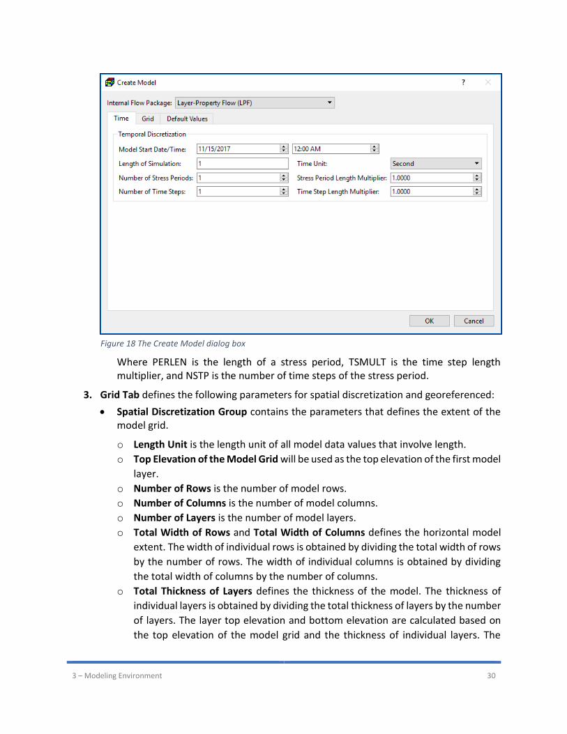
3 – Modeling Environment 30
Where PERLEN is the length of a stress period, TSMULT is the time step length multiplier, and NSTP is the number of time steps of the stress period.
3. Grid Tab defines the following parameters for spatial discretization and georeferenced:
• Spatial Discretization Group contains the parameters that defines the extent of the model grid.
o Length Unit is the length unit of all model data values that involve length.
o Top Elevation of the Model Grid will be used as the top elevation of the first model
layer.
o Number of Rows is the number of model rows.
o Number of Columns is the number of model columns.
o Number of Layers is the number of model layers.
o Total Width of Rows and Total Width of Columns defines the horizontal model
extent. The width of individual rows is obtained by dividing the total width of rows
by the number of rows. The width of individual columns is obtained by dividing
the total width of columns by the number of columns.
o Total Thickness of Layers defines the thickness of the model. The thickness of
individual layers is obtained by dividing the total thickness of layers by the number
of layers. The layer top elevation and bottom elevation are calculated based on
the top elevation of the model grid and the thickness of individual layers. The
Figure 18 The Create Model dialog box

3 – Modeling Environment 31
elevation values may be modified with Discretization > Layer Top Elevation and
Discretization > Layer Bottom Elevation.
• Georeference Group contains the parameters that are used to associate the model grid with a spatial location10.
o Georeferencing Method defines how the model grid is associated with a spatial
location.
Latitude/Longitude Coordinates of Grid Corners: If this method is selected, the
user-specified coordinates of the four model grid corners are used to place the
model grid on the map.
Grid Azimuth and Coordinates of the Lower-Left Grid Corner: If this method is
selected, the grid azimuth and the coordinates of the lower-left grid corner are
used to calculate the coordinates of the remaining grid corners. The result is
then used to place the model grid on the map. The Grid Azimuth is the angle in
degrees measured clockwise from a meridian to the axis along the model's row
direction.
o Fit to Current View: Click this button to switch the Georeferencing Method to
“Latitude/Longitude Coordinates of Grid Corners” and set the coordinates of the
grid corners to fit the current map viewer window.
4. Default Values Tab contains the default values for aquifer parameters. If a required aquifer parameter is not specified, its default value is used in the simulation.
5. OK: Click OK to create the model. If the model is created successfully, a model item will be added to the Models group on the TOC and the model item will be highlighted in yellow indicating that the new model is set as the active model. By clicking on the model item, you have access to the following settings in the Settings windows.
• General
o Name: This text string is the name of the model displayed on the TOC.
o Model ID: This text string is the unique identifier of the model and is used as the
name of a subfolder where model input/output files are stored. This subfolder
resides in the folder where the PM file is located. If the Model ID is changed, PM
will ask whether you want to rename the model’s associated subfolder.
o Notes: This is a place for you to take notes.
o Wrap Arrays: The arrays in the generated model input files will be wrapped
according to the selected option.
10 You may subsequently move and/or rotate the model grid with the Pan Tool (Section 3.5.1).
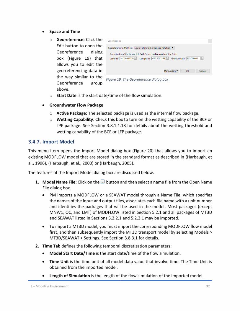
3 – Modeling Environment 32
• Space and Time
o Georeference: Click the
Edit button to open the
Georeference dialog
box (Figure 19) that
allows you to edit the
geo-referencing data in
the way similar to the
Georeference group
above.
o Start Date is the start date/time of the flow simulation.
• Groundwater Flow Package
o Active Package: The selected package is used as the internal flow package.
o Wetting Capability: Check this box to turn on the wetting capability of the BCF or
LPF package. See Section 3.8.1.1.18 for details about the wetting threshold and
wetting capability of the BCF or LFP package.
3.4.7. Import Model
This menu item opens the Import Model dialog box (Figure 20) that allows you to import an
existing MODFLOW model that are stored in the standard format as described in (Harbaugh, et
al., 1996), (Harbaugh, et al., 2000) or (Harbaugh, 2005).
The features of the Import Model dialog box are discussed below.
1. Model Name File: Click on the button and then select a name file from the Open Name File dialog box.
• PM imports a MODFLOW or a SEAWAT model through a Name File, which specifies the names of the input and output files, associates each file name with a unit number and identifies the packages that will be used in the model. Most packages (except MNW1, OC, and LMT) of MODFLOW listed in Section 5.2.1 and all packages of MT3D and SEAWAT listed in Sections 5.2.2.1 and 5.2.3.1 may be imported.
• To import a MT3D model, you must import the corresponding MODFLOW flow model first, and then subsequently import the MT3D transport model by selecting Models > MT3D/SEAWAT > Settings. See Section 3.8.3.1 for details.
2. Time Tab defines the following temporal discretization parameters:
• Model Start Date/Time is the start date/time of the flow simulation.
• Time Unit is the time unit of all model data value that involve time. The Time Unit is obtained from the imported model.
• Length of Simulation is the length of the flow simulation of the imported model.
Figure 19. The Georeference dialog box
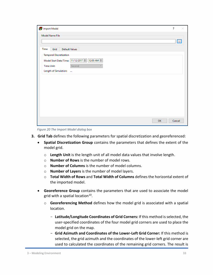
3 – Modeling Environment 33
3. Grid Tab defines the following parameters for spatial discretization and georeferenced:
• Spatial Discretization Group contains the parameters that defines the extent of the model grid.
o Length Unit is the length unit of all model data values that involve length.
o Number of Rows is the number of model rows.
o Number of Columns is the number of model columns.
o Number of Layers is the number of model layers.
o Total Width of Rows and Total Width of Columns defines the horizontal extent of
the imported model.
• Georeference Group contains the parameters that are used to associate the model grid with a spatial location10.
o Georeferencing Method defines how the model grid is associated with a spatial
location.
Latitude/Longitude Coordinates of Grid Corners: If this method is selected, the
user-specified coordinates of the four model grid corners are used to place the
model grid on the map.
Grid Azimuth and Coordinates of the Lower-Left Grid Corner: If this method is
selected, the grid azimuth and the coordinates of the lower-left grid corner are
used to calculated the coordinates of the remaining grid corners. The result is
Figure 20 The Import Model dialog box
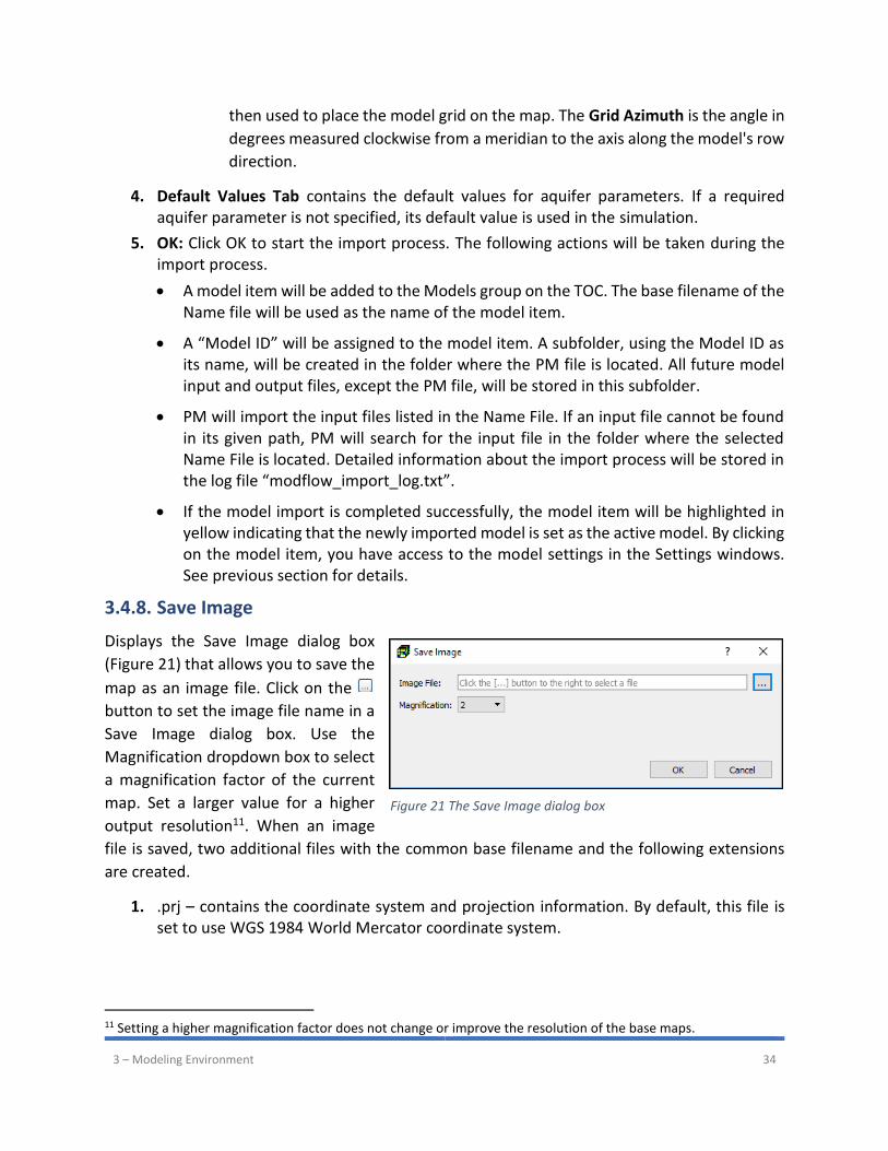
3 – Modeling Environment 34
then used to place the model grid on the map. The Grid Azimuth is the angle in
degrees measured clockwise from a meridian to the axis along the model's row
direction.
4. Default Values Tab contains the default values for aquifer parameters. If a required aquifer parameter is not specified, its default value is used in the simulation.
5. OK: Click OK to start the import process. The following actions will be taken during the import process.
• A model item will be added to the Models group on the TOC. The base filename of the Name file will be used as the name of the model item.
• A “Model ID” will be assigned to the model item. A subfolder, using the Model ID as its name, will be created in the folder where the PM file is located. All future model input and output files, except the PM file, will be stored in this subfolder.
• PM will import the input files listed in the Name File. If an input file cannot be found in its given path, PM will search for the input file in the folder where the selected Name File is located. Detailed information about the import process will be stored in the log file “modflow_import_log.txt”.
• If the model import is completed successfully, the model item will be highlighted in yellow indicating that the newly imported model is set as the active model. By clicking on the model item, you have access to the model settings in the Settings windows. See previous section for details.
3.4.8. Save Image
Displays the Save Image dialog box
(Figure 21) that allows you to save the
map as an image file. Click on the
button to set the image file name in a
Save Image dialog box. Use the
Magnification dropdown box to select
a magnification factor of the current
map. Set a larger value for a higher
output resolution11. When an image
file is saved, two additional files with the common base filename and the following extensions
are created.
1. .prj – contains the coordinate system and projection information. By default, this file is set to use WGS 1984 World Mercator coordinate system.
11 Setting a higher magnification factor does not change or improve the resolution of the base maps.
Figure 21 The Save Image dialog box
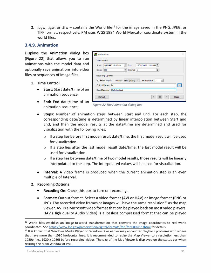
3 – Modeling Environment 35
2. .pgw, .jgw, or .tfw – contains the World file12 for the image saved in the PNG, JPEG, or TIFF format, respectively. PM uses WGS 1984 World Mercator coordinate system in the world files.
3.4.9. Animation
Displays the Animation dialog box
(Figure 22) that allows you to run
animations with the model data and
optionally save animations into video
files or sequences of image files.
1. Time Control
• Start: Start date/time of an animation sequence.
• End: End date/time of an animation sequence.
• Steps: Number of animation steps between Start and End. For each step, the corresponding date/time is determined by linear interpolation between Start and End, and then the model results at the date/time are determined and used for visualization with the following rules:
o If a step lies before first model result date/time, the first model result will be used
for visualization.
o If a step lies after the last model result date/time, the last model result will be
used for visualization.
o If a step lies between date/time of two model results, those results will be linearly
interpolated to the step. The interpolated values will be used for visualization.
• Interval: A video frame is produced when the current animation step is an even multiple of Interval.
2. Recording Options
• Recoding On: Check this box to turn on recording.
• Format: Output format. Select a video format (AVI or HAV) or image format (PNG or JPG). The recorded video frames or images will have the same resolution13 as the map viewer. AVI is a Microsoft video format that can be played back on most video players. HAV (High quality Audio Video) is a lossless compressed format that can be played
12 World files establish an image-to-world transformation that converts the image coordinates to real-world coordinates. See https://www.loc.gov/preservation/digital/formats/fdd/fdd000287.shtml for details. 13 It is known that Windows Media Player on Windows 7 or earlier may encounter playback problems with videos that have more than 1080 horizontal lines. It is recommended to resize the Map Viewer to a resolution less than 1080p (i.e., 1920 x 1080) before recording videos. The size of the Map Viewer is displayed on the status bar when resizing the Main Window of PM.
Figure 22 The Animation dialog box

3 – Modeling Environment 36
back with the free Imagen multimedia player and can be converted to other formats with the VideoMach software. Both software packages are available on www.gromada.com.
• Frame Rate: number of frames per second when a recorded video file is played back. The total duration (in seconds) of the recorded video file is approximately Steps/Interval/Frame Rate.
• Output Folder: click the button to select a folder where the video or image files will be saved.
• Base Filename: This the base filename (i.e., without a file extension) of output files. The appropriate file extension will be determined based on the selected format, and appended to the base filename.
3. : Play the animation sequence forwards from Start to End. Output file(s) will be created or updated if Recording On is checked. Make sure that the existing output file(s) are not opened in other applications that may prevent those file(s) from being updated.
4. : Play the animation sequence backwards from End to Start. Output file(s) will be created or updated if Recording On is checked. Make sure that the existing output file(s) are not opened in other applications that may prevent those file(s) from being updated.
Default: Click this button to set default values to all controls, i.e., Start to the model start date/time, End to the model end date/time, Steps to 10, Recording off, Format to HAV, Frame Rate to 4, etc.
3.4.10. Print
Opens the Print dialog box (Figure 23). Its right-hand panel provides a print preview. You can
adjust the print settings with the controls on the left-hand panel. Optionally, you can enter a
caption and load a logo (saved in the .png or .jpg formats). Click on the Print button on the Top-
Left corner of the dialog box to print.
3.4.11. Preferences
Displays the Preferences dialog box with four tabs as follows.
1. Path Tab: This tab contains a table that defines the file paths of following supported models and/or applications. To change the path of a specific model/application, double-click on the respective path and then select an executable file from the Select Model Executable File dialog box.
• MODFLOW-2005: MODFLOW is the USGS's three-dimensional (3D) finite-difference groundwater model. MODFLOW is considered an international standard for simulating and predicting groundwater conditions and groundwater/surface-water interactions. For details, visit https://water.usgs.gov/ogw/modflow/index.html
• MODFLOW-NWT: The USGS MODFLOW-NWT is a Newton-Raphson formulation for MODFLOW-2005 to improve solution of unconfined groundwater-flow problems.
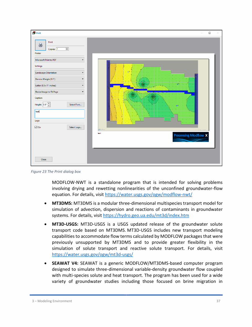
3 – Modeling Environment 37
MODFLOW-NWT is a standalone program that is intended for solving problems involving drying and rewetting nonlinearities of the unconfined groundwater-flow equation. For details, visit https://water.usgs.gov/ogw/modflow-nwt/
• MT3DMS: MT3DMS is a modular three-dimensional multispecies transport model for simulation of advection, dispersion and reactions of contaminants in groundwater systems. For details, visit https://hydro.geo.ua.edu/mt3d/index.htm
• MT3D-USGS: MT3D-USGS is a USGS updated release of the groundwater solute transport code based on MT3DMS. MT3D-USGS includes new transport modeling capabilities to accommodate flow terms calculated by MODFLOW packages that were previously unsupported by MT3DMS and to provide greater flexibility in the simulation of solute transport and reactive solute transport. For details, visit https://water.usgs.gov/ogw/mt3d-usgs/
• SEAWAT V4: SEAWAT is a generic MODFLOW/MT3DMS-based computer program designed to simulate three-dimensional variable-density groundwater flow coupled with multi-species solute and heat transport. The program has been used for a wide variety of groundwater studies including those focused on brine migration in
Figure 23 The Print dialog box

3 – Modeling Environment 38
continental aquifers as well as those focused on saltwater intrusion in coastal aquifers. For details, visit https://water.usgs.gov/ogw/seawat/
• PEST: This is the standard version of PEST that runs in a single thread. PEST is the industry standard software package for parameter estimation and uncertainty analysis of complex environmental and other computer models. For details, visit http://www.pesthomepage.org/.
• BeoPEST: BeoPEST is a special version of Parallel PEST inspired by Beowulf Clusters. A Beowulf Cluster contains several computers that are tied together using a reasonably fast network. When running BeoPEST within PM on a multicore computer, it is configured to run solution agents on individual CPU cores to accelerate the parameter estimation process (by solving the Jacobian matrix parallelly). For details, visit http://www.pesthomepage.org/BEOPEST.php
• PESTCHEK: PESTCHEK is a utility program that checks an entire PEST input dataset for correctness and consistency. For details and for additional utilities, visit http://www.pesthomepage.org/PEST_Utilities.php
• MODPATH: MODPATH is a particle-tracking post-processing program designed to work with MODFLOW. The included MODPATH version 7 is the fourth major release since its original publication. For details, visit https://water.usgs.gov/ogw/modpath/
• Zone Budget: ZONEBUDGET is a program for computing subregional water budgets for MODFLOW. For details, visit https://water.usgs.gov/nrp/gwsoftware/zonebud3/zonebudget3.html
• Text Editor: The text editor is used to display simulation log and certain result files that are saved in the text format. Most text editors, such as NotePad++ or EmEditor, may be used instead of the Windows’s default Notepad application.
2. Visual Tab
• Popup Label Color and Font Size: When the mouse hovers over some visual objects, such as flow vectors, their detailed information can be displayed with a pop-up label. The color and font size of the pop-up label are defined here. To change a color, click
on the button and then pick a color from the Select Color dialog box.
• Show Scale: Check this box to display the scale on the lower-left corner of the Map Viewer; clear this box to hide the scale.
• Background Color: This defines the background color of the Map Viewer.
• Ground Surface Elevation Unit: This defines the unit of the ground surface elevation at the mouse cursor’s location on the map. Elevation values are provided for reference purposes only and do not represent precisely measured or surveyed values.
• Use current view as my default view: Click this button to set the current view extent as the default view extent when PM is started. This button is deactivated when the
button on the toolbar is depressed.
3 – Modeling Environment 39
• Polyline Opacity and Color: These controls define the color and opacity of polylines created by the Polyline input method (Section 3.3.2.2). The value of opacity ranges from 0 to 100, with 0 being transparent and 100 being opaque.
• Polygon Opacity and Color: These controls define the color and opacity of polygons created by the Polygon input method (Section 3.3.2.3).
• Grid Cursor Opacity and Color: These controls define the color and opacity of the grid cursor. For details about the grid cursor, see Sections 3.2 and 3.3.2.
• Highlight Opacity and Auto Clear: Within the data editor (Section 3.3.2), you can double-click on a cell to highlight all other cells that have the same value as the clicked cell. The value of Highlight Opacity controls the opacity of the highlight mask. The color of the highlight mask changes with repeated double-clicks. When the Auto Clear box is checked, the highlight mask will be cleared automatically whenever the model grid is drawn or redrawn.
• Value Display Precision: This is the maximum number of significant digits that is used to display model values on the Properties window.
• Layer Elevation: When the top of bottom elevation of a model layer is modified, the elevation of the neighboring layers will be automatically adjusted to match when the Auto Adjust box is checked.
3. Network Proxy Tab
• Proxy Type:
o No Proxy: Choose this if you don’t want to use a proxy.
o Auto-Detect: Choose this if you want PM to automatically detect the proxy
settings.
o Manual: Choose this if you want to configure the proxy settings manually. PM uses
the SOCKS5 protocol to connect to the proxy server.
• Proxy Settings: If the selected Proxy Type is Manual, you need to provide the proxy server details as follows.
o Host: address of the proxy server
o Port: port of the proxy server
o User Name: user name for proxy authentication
o Password: Password for proxy authentication.
4. Misc. Tab
• Before Running a Model: Defines the action to be taken before a model run is commenced.
• After Deleting a Model: Defines the action to be taken after a model is deleted.
3 – Modeling Environment 40
• PEST Version: Defines the PEST version to be used for the parameter estimation process.
• Number of Agents: This is the number of BeoPEST instances that are used to solve the parameter estimation problem. The default value is the number of physical CPU cores of the computer.
• Port: This is the TCP/IP port number that is used by BeoPEST to communicate between the master and agent instances. The port number can be any unused port on the host where the master is run. Port numbers are positive integers between 1024 and 65536. Typically, a port number such as 4004 is unused.
• Output Width: This is the output width (in pixels) of charts.
• Maximum Number of Backups: This is the maximum number of backups of the currently loaded PM file. A backup is of the loaded PM file is created before it is saved.
3.5. Tools Menu
3.5.1. Pan Tool
To activate the Pan Tool, click on the Pan Tool icon in the toolbar or select Tools > Pan Tool.
The Pan tool has the following major functions.
1. Move the map view in any direction: Place the mouse cursor within the Map Viewer and drag to move the view. Alternatively, the w, e, d, c, x, z, a, and q keys can be used to move the view towards the north, northeast, east, southeast, south, southwest, west, and northwest, respectively.
2. Move the grid cursor:
• Move the grid cursor to a cell by left-clicking on that cell.
• Drag the grid cursor with the mouse.
• Use the arrow keys to move horizontally. Use the Shift-PageUp and Shift-PageDown keys to move to the upper or lower layer.
3. Move the model grid with shift-drag: Place the mouse cursor over the grid cursor, press and hold the Shift-key and the left mouse button, move the mouse to drag the model grid, and then release the Shift -key and left mouse button to place the model grid.
4. Rotate the model grid with ctrl-drag: Place the mouse cursor over the grid cursor, press and hold the Ctrl-key and left mouse button, move the mouse to rotate the model grid, and then release the Ctrl-key and left mouse button to place the model grid. The center of rotation is the lower-left corner of the unrotated grid.
5. Zoom in: Place the mouse cursor within the Map Viewer, press and hold the right button, and move the mouse forward. Release the button when you reach the desired zoom level. Alternatively, if your mouse has a scroll wheel, it can be used to zoom in by scrolling it forward.
3 – Modeling Environment 41
6. Zoom out: Place the mouse cursor within the Map Viewer, press and hold the right mouse button, and move the mouse backward. Release the button when the desired zoom level is reached. Alternatively, if your mouse has a scroll wheel, it can be used to zoom out by scrolling it backward.
3.5.2. Zoom Tool
To activate the Zoom Tool, click on the Zoom Tool icon in the toolbar or select Tools > Zoom
Tool. The Zoom tool has the following major functions.
1. Move the map view in any direction: Press the arrow keys to move the map view toward their respective directions. The w, e, d, c, x, z, a, and q keys can also be used to move the view towards north, northeast, east, southeast, south, southwest, west, and northwest, respectively.
2. Move the grid cursor to a desired cell by left-clicking on that cell.
3. Move the model grid with shift-drag: Same as the Pan tool described above.
4. Rotate the model grid with ctrl-drag: Same as the Pan tool described above.
5. Zoom in: To zoom in, position the mouse cursor on the corner of the desired area, press and hold down the left button, drag the mouse cursor to the opposite corner of the desired area, and release the left button. If your mouse has a scroll wheel, it can be used to zoom in by scrolling it forward.
6. Zoom out: If your mouse has a scroll wheel, it can be used to zoom out by scrolling it backward.
3.5.3. Observation Tool
The Observation tool is used to define the observation points, and observation values pertaining
the observation points. The data can be used by PEST for model calibration or used by the Scatter
and Line charts. To activate the Observation Tool, click on the Observation Tool icon in the
toolbar or select Tools > Observation Tool.
1. Add observation points: To add observation points to the active model, move to the desired layer with or buttons on the toolbar and then click on the desired locations on the Map Viewer. The color of the observation points matches with the color assigned to the layer (see Section 3.6.3 for the Layer Properties).
2. Remove an observation point: Right-click on the observation point in the Map Viewer to open the Observation dialog box (Figure 24), and then click Delete in the dialog box to delete the selected point.
3. Move observation points: Place the mouse cursor over an observation point, press and hold the left mouse button, move the mouse to drag the observation point, and then release the left mouse button to place the observation point.
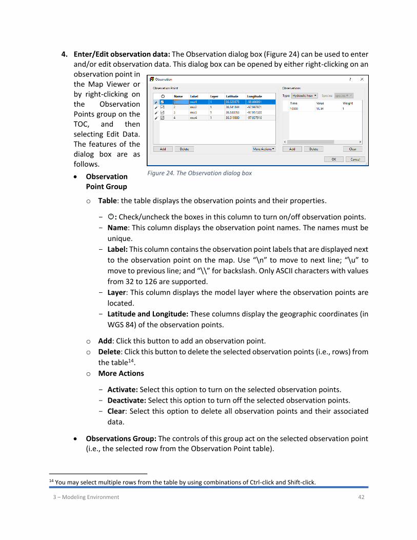
3 – Modeling Environment 42
4. Enter/Edit observation data: The Observation dialog box (Figure 24) can be used to enter and/or edit observation data. This dialog box can be opened by either right-clicking on an observation point in the Map Viewer or by right-clicking on the Observation Points group on the TOC, and then selecting Edit Data. The features of the dialog box are as follows.
• Observation Point Group
o Table: the table displays the observation points and their properties.
: Check/uncheck the boxes in this column to turn on/off observation points.
Name: This column displays the observation point names. The names must be
unique.
Label: This column contains the observation point labels that are displayed next
to the observation point on the map. Use “\n” to move to next line; “\u” to
move to previous line; and “\\” for backslash. Only ASCII characters with values
from 32 to 126 are supported.
Layer: This column displays the model layer where the observation points are
located.
Latitude and Longitude: These columns display the geographic coordinates (in
WGS 84) of the observation points.
o Add: Click this button to add an observation point.
o Delete: Click this button to delete the selected observation points (i.e., rows) from
the table14.
o More Actions
Activate: Select this option to turn on the selected observation points.
Deactivate: Select this option to turn off the selected observation points.
Clear: Select this option to delete all observation points and their associated
data.
• Observations Group: The controls of this group act on the selected observation point (i.e., the selected row from the Observation Point table).
14 You may select multiple rows from the table by using combinations of Ctrl-click and Shift-click.
Figure 24. The Observation dialog box
3 – Modeling Environment 43
o Type: This dropdown box is used to select the type of the observation data.
o Species: This This dropdown box is activated only if the Type is Concentration and
is used to select the specifies to which the observation data belong.
o Table: The table displays the observation data.
Time: Observation time, expressed in the elapsed time (in the model time unit)
since the start of the simulation.
Value: Observed value of the selected Type.
Weight: The Weight of an observation gives a relative confidence level of the
observed value. The higher the Weight value, the better is the measurement.
The weight can be set at zero if needed (meaning that the observation takes no
part in the calculation of the objective function during a parameter estimation
process), but it must not be negative. Refer to the PEST User Manual (Doherty,
2016) for the function of weights in the parameter estimation process.
o Add: Click this button to add a row to the Table.
o Delete: Click this button to delete the selected rows from the Table.
o Clear: Click this button to delete all observation data from the Table.
5. Export/Import observation points:
• Export to Shapefile: Right-click on the Observation Points group on the TOC, select Export to Shapefile from the popup menu, and then select a shapefile in the Save As dialog box.
• Export to Excel File: Right-click on the Observation Points group on the TOC, select Export to Excel File from the popup menu, and then select an Excel file in the Save As dialog box. The Excel file contains the observation points and observation data. Its format is described in Section 5.1.1.
• Import from Excel file: Right-click on the Observation Points group on the TOC, select Import from Excel File from the popup menu, and then select an Excel file in the Open File dialog box. The Excel file must be saved in the format described in Section 5.1.1.
3.5.4. MODPATH Tool
The MODPATH Tool may be accessed only when the active layer is a MODPATH instance. This
tool is used to define starting locations for particle tracking. For details of running MODPATH, see
Section 4.2.4.
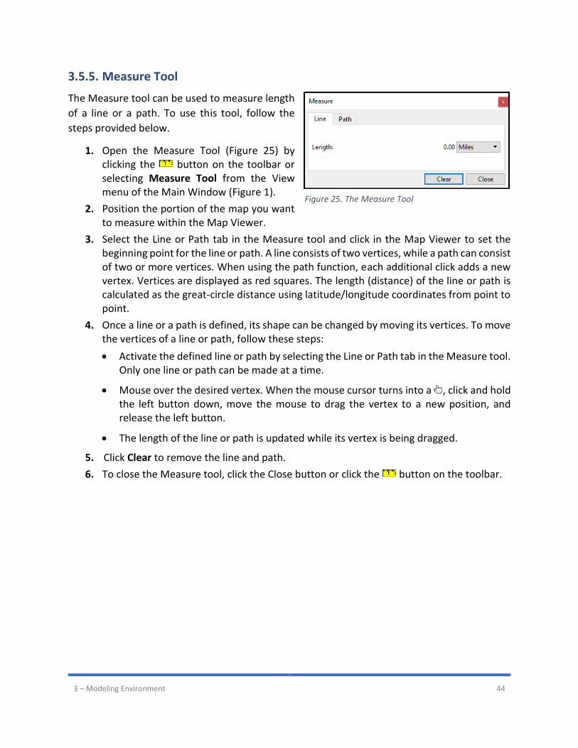
3 – Modeling Environment 44
3.5.5. Measure Tool
The Measure tool can be used to measure length
of a line or a path. To use this tool, follow the
steps provided below.
1. Open the Measure Tool (Figure 25) by clicking the button on the toolbar or selecting Measure Tool from the View menu of the Main Window (Figure 1).
2. Position the portion of the map you want to measure within the Map Viewer.
3. Select the Line or Path tab in the Measure tool and click in the Map Viewer to set the beginning point for the line or path. A line consists of two vertices, while a path can consist of two or more vertices. When using the path function, each additional click adds a new vertex. Vertices are displayed as red squares. The length (distance) of the line or path is calculated as the great-circle distance using latitude/longitude coordinates from point to point.
4. Once a line or a path is defined, its shape can be changed by moving its vertices. To move the vertices of a line or path, follow these steps:
• Activate the defined line or path by selecting the Line or Path tab in the Measure tool. Only one line or path can be made at a time.
• Mouse over the desired vertex. When the mouse cursor turns into a , click and hold the left button down, move the mouse to drag the vertex to a new position, and release the left button.
• The length of the line or path is updated while its vertex is being dragged.
5. Click Clear to remove the line and path.
6. To close the Measure tool, click the Close button or click the button on the toolbar.
Figure 25. The Measure Tool
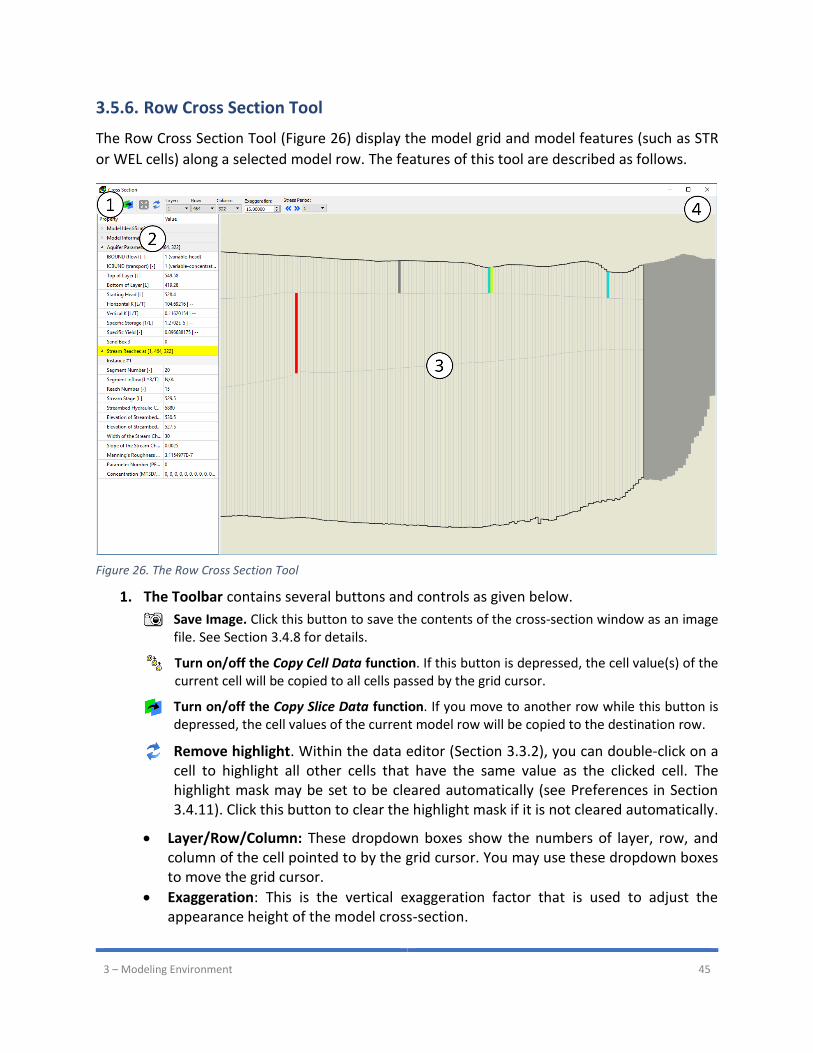
3 – Modeling Environment 45
3.5.6. Row Cross Section Tool
The Row Cross Section Tool (Figure 26) display the model grid and model features (such as STR
or WEL cells) along a selected model row. The features of this tool are described as follows.
1. The Toolbar contains several buttons and controls as given below.
Save Image. Click this button to save the contents of the cross-section window as an image file. See Section 3.4.8 for details.
Turn on/off the Copy Cell Data function. If this button is depressed, the cell value(s) of the current cell will be copied to all cells passed by the grid cursor.
Turn on/off the Copy Slice Data function. If you move to another row while this button is depressed, the cell values of the current model row will be copied to the destination row.
Remove highlight. Within the data editor (Section 3.3.2), you can double-click on a cell to highlight all other cells that have the same value as the clicked cell. The highlight mask may be set to be cleared automatically (see Preferences in Section 3.4.11). Click this button to clear the highlight mask if it is not cleared automatically.
• Layer/Row/Column: These dropdown boxes show the numbers of layer, row, and column of the cell pointed to by the grid cursor. You may use these dropdown boxes to move the grid cursor.
• Exaggeration: This is the vertical exaggeration factor that is used to adjust the appearance height of the model cross-section.
Figure 26. The Row Cross Section Tool
3 – Modeling Environment 46
• Stress Period: The dropdown box displays the current stress period. You may use the dropdown box to move to another period. Alternatively, click the or button to move to the previous or next stress period, respectively.
• Time Step: The dropdown box displays the current time step within the selected Stress Period. You may use the dropdown box to move to another time step. Alternatively, click the or button to move to the previous or next time step, respectively.
2. The Property Window: This window displays the meta data of the model. If a model data or package, such as Specific Storage or STR, is being edited, this window displays the meta data of the model along with the properties of the cell pointed to by the grid cursor. The cell data that is currently being edited is highlighted in yellow.
3. The Cross-Section Window: This window displays the model grid and model cell features along the model row specified by the Row dropdown box. The cell that is pointed to by the grid cursor is the active cell.
• Display Settings: The display settings of the model grid are defined by the Settings window for model grid (Figure 101). That is, the settings are the same as those for the model grid on the Map Viewer. You must adjust the settings before opening the Cross-section tool.
• Move the cross-section view in any direction: Place the mouse cursor within the window and then drag to move the view. Alternatively, the w, e, d, c, x, z, a, and q keys can be used to move the view towards the north, northeast, east, southeast, south, southwest, west, and northwest, respectively.
• Move the grid cursor. There are several ways to move the grid cursor. o Move the grid cursor to a cell by left-clicking on that cell.
o Drag the grid cursor with the mouse.
o Use the arrow keys to move horizontally. Use the Shift-PageUp and Shift-
PageDown keys to move to the adjacent rows.
o Use the Layer/Row/Column dropdown boxes on the toolbar.
• Zoom in: Place the mouse cursor within the window, press and hold the right button, and move the mouse forward. Release the button when you reach the desired zoom level. Alternatively, if your mouse has a scroll wheel, it can be used to zoom in by scrolling it forward.
• Zoom out: Place the mouse cursor within the window, press and hold the right mouse button, and move the mouse backward. Release the button when the desired zoom level is reached. Alternatively, if your mouse has a scroll wheel, it can be used to zoom out by scrolling it backward.
• Edit Cell data: If you invoke the Row Cross-Section Tool while editing a certain model data, you may edit the cell data by right-clicking on the cell of interest. You can double-click on a cell (or press the Insert key) to highlight all other cells that have the same cell value as the clicked cell.
3 – Modeling Environment 47
4. Close the Tool. To close the tool, click the X button located on its upper-right corner. After closing this tool, the grid cursor on the Map Viewer will be moved to the cell pointed to by the Layer/Row/Column dropdown boxes of this tool. The model on the Map Viewer will be redrawn if necessary.
3.5.7. Pin Tool
Select Tools > Pin Tool or push down the button on the toolbar to disable map pan and zoom
with the mouse.
3.5.8. Rotation Tool
Select Tools > Rotation Tool or push down the button on the toolbar to orientate the display
of the active model grid horizontally. All other visual objects, including other models, will be
rotated with the active model grid accordingly.
3.5.9. Finish Edit
Click on the button on the toolbar to finishing editing the grid or the model data. If changes
have been made, you will be prompted to save or discard the changes.
3.5.10. Cell-by-Cell Tool
Within the Data Editor, you may select Tools > Cell-by-Cell Tool or push down the button on
the toolbar to switch to the Cell-by-Cell input method. See section 3.3.2.1 for details.
3.5.11. Polyline Tool
Within the Data Editor, you may select Tools > Polyline Tool or push down the button on the
toolbar to switch to the Polyline input method. See section 3.3.2.2 for details.
3.5.12. Polygon Tool
Within the Data Editor, you may select Tools > Polygon Tool or push down the button on the
toolbar to switch to the Polygon input method. See section 3.3.2.3 for details.
3.5.13. Cell Copy
Within the Data Editor, you may select Tools > Cell Copy or push down the button on the
toolbar to turn on the Copy Cell Data function. If this button is depressed, the cell value(s) of the
current cell will be copied to all cells passed by the grid cursor.
3.5.14. Layer Copy
Within the Data Editor, you may select Tools > Layer Copy or push down the button on the
toolbar to turn on the Copy Layer Data function. If you move to another layer while this button
3 – Modeling Environment 48
is depressed, the cell values, polylines, and polygons of the current layer will be copied to the
destination layer.
3.5.15. Grid Size Copy
Within the Grid Editor, you may select Tools > Grid Size Copy or push down the button on the
toolbar to turn on the Copy Grid Size function. If this button is depressed, the column and row
width of the current cell will be copied to all cells passed by the grid cursor.
3.5.16. Grid Split Copy
Within the Grid Editor, you may select Tools > Grid Split Copy or push down the button on the
toolbar to turn on the Copy Grid Split Factor function. If this button is depressed, the column and
row split factors of the current cell will be copied to all cells passed by the grid cursor
3.5.17. Tools > Data Menu
Within the Data Editor, you may use this menu to manipulate cell-by-cell data of the current layer
and/or the entire model.
1. Matrix: Select this menu item to open the Matrix dialog box that displays cell values in a table. This function is available only when editing IBOUND, ICBUND, Layer Top/Bottom elevations, aquifer parameters, concentration values, and certain flow packages with matrix-based input data, such as Evapotranspiration or Recharge packages. The features of the Matrix dialog box are as follows.
• Table: The table displays cell values of the selected parameter. The columns and rows of the table correspond to the model columns and rows. You may edit the value of a cell by clicking on the cell and then typing in the desired value. You may edit the values of a group of cells by selecting those cells with the mouse, and then typing in the desired value.
• Parameter: The cell values of the selected parameter are displayed in the table.
• Column Width: This defines the display width of the columns of the table.
• Statistics: This line contains the statistics of the displayed values.
2. Reset: Select this menu item to open the Reset dialog box, which is used to assign uniform cell values to the current model layer or to the entire model.
The options Apply to the entire model and Apply to the current layer are available when editing IBOUND, ICBUND, layer top/bottom elevations, aquifer parameters, or concentration values.
• Apply to the entire model: If this option is selected, the specified value(s) in the Reset Matrix dialog box will be applied to all cells of the entire model.
• Apply to the current layer: If this option is selected, the specified value(s) in the Reset Matrix dialog box will be applied to all cells of the current model layer.

3 – Modeling Environment 49
3. Modify: Open the Modify Data dialog box (Figure 27). This allows you to modify or display cell values of the current layer.
• Parameter: The modification operation is applied to the selected parameter.
• Search Range: The modification operation will be applied to the cells with the selected parameter values lying within the given search range.
• Value: The user-specified value that is used to modify the cell values.
• Manipulation: The final cell values15 is obtained by cell-by-cell calculation according to the selected manipulation rule.
o None (display only): No modification takes place.
o Replace: Final cell value = the user-specified value.
o Add: Final cell value = current cell value + the user-specified value.
o Subtract: Final cell value = current cell value - the user-specified value.
o Multiply: Final cell value = current cell value × the user-specified value.
o Divide: For a non-zero user-specified value, final cell value = current cell value /
the user-specified value. If the user-specified value equals to zero, the cell value
remains unchanged.
o Minimum: Final cell value = minimum of the user-specified value and current cell
value.
o Maximum: Final cell value = maximum of the user-specified value and current cell
value.
4. Import: Open the Import Data dialog box (Figure 28) that allows you to import cell values from several types of files.
• File: Click the button to select a file to be imported. After selecting a file, PM will attempt to determine its file type by examines its contents. If a supported file type is determined, the File Type dropdown box (see below) will be updated accordingly.
• Parameter: The import operation will be applied to the selected parameter.
15If the selected parameter does not allow zero or negative cell values, such as density or hydraulic conductivity, the final cell value will be set to 1e-20, if the modified value is less than or equal to zero. If the selected parameter is Parameter Number, the final cell value is limited between 0 and 10000.
Figure 27. The Modify Data dialog box
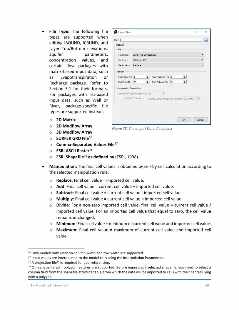
3 – Modeling Environment 50
• File Type: The following file types are supported when editing IBOUND, ICBUND, and Layer Top/Bottom elevations, aquifer parameters, concentration values, and certain flow packages with matrix-based input data, such as Evapotranspiration or Recharge package. Refer to Section 5.1 for their formats. For packages with list-based input data, such as Well or River, package-specific file types are supported instead.
o 2D Matrix
o 2D Modflow Array
o 3D Modflow Array
o SURFER GRD File16
o Comma-Separated Values File17
o ESRI ASCII Raster18
o ESRI Shapefile19 as defined by (ESRI, 1998).
• Manipulation: The final cell values is obtained by cell-by-cell calculation according to the selected manipulation rule:
o Replace: Final cell value = imported cell value.
o Add: Final cell value = current cell value + imported cell value.
o Subtract: Final cell value = current cell value - imported cell value.
o Multiply: Final cell value = current cell value × imported cell value.
o Divide: For a non-zero imported cell value, final cell value = current cell value /
imported cell value. For an imported cell value that equal to zero, the cell value
remains unchanged.
o Minimum: Final cell value = minimum of current cell value and imported cell value.
o Maximum: Final cell value = maximum of current cell value and imported cell
value.
16 Only models with uniform column width and row width are supported. 17 Input values are interpolated to the model cells using the Interpolation Parameters. 18 A projection file38 is required for geo-referencing. 19 Only shapefile with polygon features are supported. Before importing a selected shapefile, you need to select a column field from the shapefile attribute table, from which the data will be imported to cells with their centers lying with a polygon.
Figure 28. The Import Data dialog box

3 – Modeling Environment 51
• Position: Define the subgrid (by default, the entire grid) where the data will be imported to.
o If a 2D Matrix, 2D Modflow Array, or 3D Modflow Array is used, the matrix values
will be imported to the defined subgrid. The value located at [i, j] of the imported
matrix will be imported to the cell located at [i + StartRow - 1, j + StartColumn - 1],
if the cell location is valid.
o If a Comma-Separated Values File or an ESRI ASCII Raster is use, the input values
will be interpolated to the cells of the subgrid. The resulting matrix with the
interpolated values will then be imported in the same way as described above.
• Interpolation Parameters: These parameters are used to interpolate the input values from the Comma-Separated Values file or the ESRI ASCII Raster file to the model grid. The interpolation process is based on a weighted method. In this method, the grid value 𝐶𝑖𝑗 at the cell [j, i] is the weighted average of surrounding data values, i.e.,
𝐶𝑖𝑗 = ∑ 𝐶𝑘𝑊𝑘(𝑟)𝑛𝑘=1 ∑ 𝑊𝑘(𝑟)𝑛
𝑘=1⁄ ,
where 𝐶𝑘 is the measured value at the kth measuring point, 𝑛 the number of surrounding data values, 𝑊𝑘(𝑟) is the weighting function, and 𝑟 the distance from the grid point to the measuring point. The key component of a weighted method is the weighting function. A survey of weighting functions is presented by (Goodin, et al., 1979). In PM, the weighting function developed by Shepard (1968) is used, which improves the pure inverse distance weighting method by adding functions to dynamically determine (1) the radius of influence based on data density and distribution, and (2) the weighting factors based on distance between model cells and data points in the interpolation algorithm.
o Radius and Preferred Number of Neighboring Points (PNP): These values
determine the neighboring data points that should be used to estimate the value
at that cell with the following rules:
The number of points within the Radius (NPR) of the grid cell is determined by
PM with a fast search algorithm.
The number of neighboring points (NP) used by the Shepard’s method to
estimate the value at the grid cell is determined as follows:
𝑁𝑃 = 𝑀𝑖𝑛𝑁𝑃 𝑖𝑓 𝑁𝑃𝑅 < 𝑀𝑖𝑛𝑁𝑃,
𝑁𝑃 = 𝑁𝑃𝑅 𝑖𝑓 𝑀𝑖𝑛𝑁𝑃 < 𝑁𝑃𝑅 < 𝑀𝑎𝑥𝑁𝑃, 𝑎𝑛𝑑
𝑁𝑃 = 𝑀𝑎𝑥𝑁𝑃 𝑖𝑓 𝑁𝑃𝑅 > 𝑀𝑎𝑥𝑁𝑃,
where 𝑀𝑖𝑛𝑁𝑃 = 𝑃𝑁𝑃 × 2 3⁄ and 𝑀𝑎𝑥𝑁𝑃 = 𝑃𝑁𝑃 × 4 3⁄
The radius used by the Shepard’s method is the radius that encompasses those
NP points next to the grid cell.
o Logarithmic Transform: Check this box to log-transform the input values prior to performing interpolation. This is typically necessary if the input data is positively
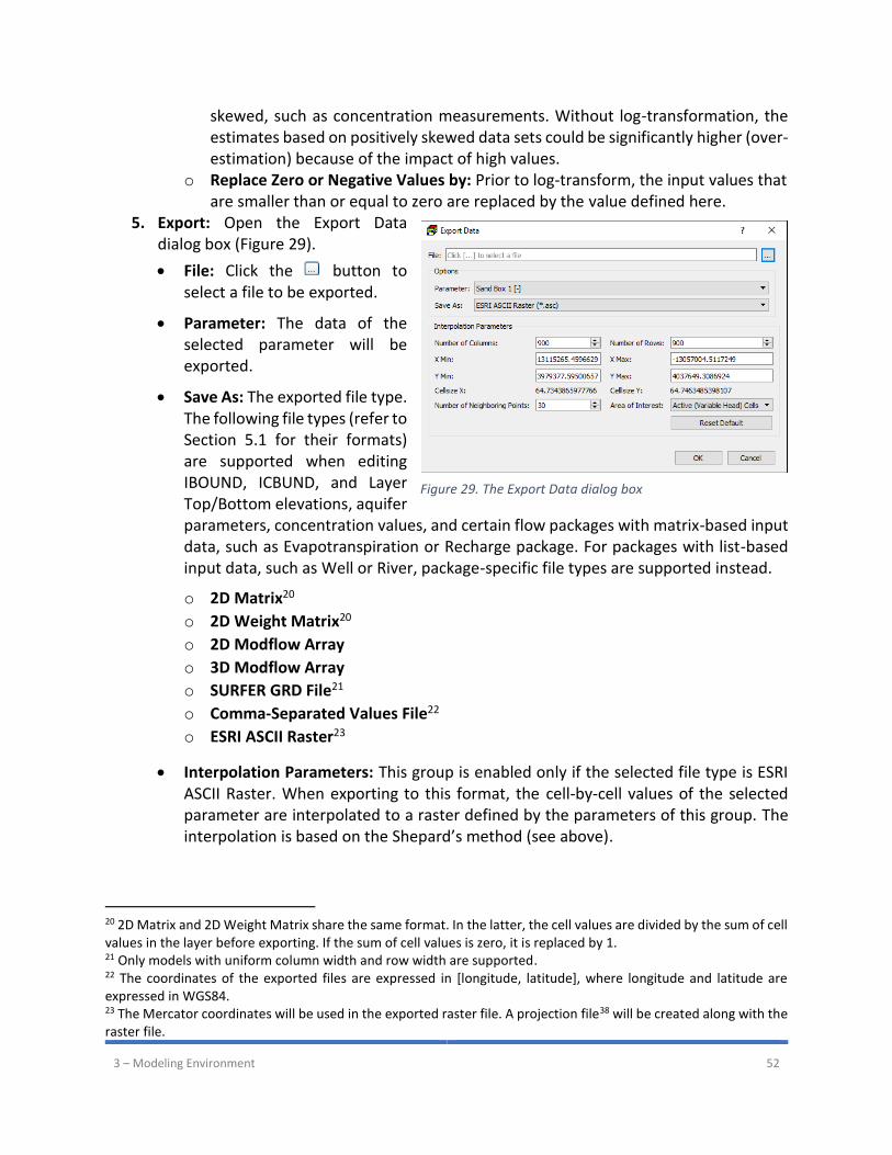
3 – Modeling Environment 52
skewed, such as concentration measurements. Without log-transformation, the estimates based on positively skewed data sets could be significantly higher (over-estimation) because of the impact of high values.
o Replace Zero or Negative Values by: Prior to log-transform, the input values that are smaller than or equal to zero are replaced by the value defined here.
5. Export: Open the Export Data dialog box (Figure 29).
• File: Click the button to select a file to be exported.
• Parameter: The data of the selected parameter will be exported.
• Save As: The exported file type. The following file types (refer to Section 5.1 for their formats) are supported when editing IBOUND, ICBUND, and Layer Top/Bottom elevations, aquifer parameters, concentration values, and certain flow packages with matrix-based input data, such as Evapotranspiration or Recharge package. For packages with list-based input data, such as Well or River, package-specific file types are supported instead.
o 2D Matrix20
o 2D Weight Matrix20
o 2D Modflow Array
o 3D Modflow Array
o SURFER GRD File21
o Comma-Separated Values File22
o ESRI ASCII Raster23
• Interpolation Parameters: This group is enabled only if the selected file type is ESRI ASCII Raster. When exporting to this format, the cell-by-cell values of the selected parameter are interpolated to a raster defined by the parameters of this group. The interpolation is based on the Shepard’s method (see above).
20 2D Matrix and 2D Weight Matrix share the same format. In the latter, the cell values are divided by the sum of cell values in the layer before exporting. If the sum of cell values is zero, it is replaced by 1. 21 Only models with uniform column width and row width are supported. 22 The coordinates of the exported files are expressed in [longitude, latitude], where longitude and latitude are expressed in WGS84. 23 The Mercator coordinates will be used in the exported raster file. A projection file38 will be created along with the raster file.
Figure 29. The Export Data dialog box
3 – Modeling Environment 53
o Number of Columns and Number of Rows: The exported raster will have the
defined numbers of columns and rows.
o X Min, X Max, Y Min, and Y Max: These are respectively the minimum and
maximum X and Y coordinates (expressed in the Mercator coordinate system) of
the raster. The default values cover the entire model grid.
o Cellsize X and Cellsize Y: These are respectively the column and row widths of the
raster. These values are calculated based on the input values given above.
o Number of neighboring points: This defines the number of neighboring data
points that should be used to estimate the value at a raster cell.
o Area of Interest: Cell-by-cell values are interpolated to the raster points within the
selected area of interest and Nodata_Value (-1E20) is assigned to all other raster
points. The results of the options “All” and “Model Bounding Box” are the same if
the model grid is not rotated (or one of the model grid axis is parallel to a
meridian).
o Reset Default: Click this button to reset the values of numbers of columns and
rows, as well as X Min, X Max, Y Min, and Y Max to their default settings.
3.5.18. Tools > Package Menu
1. Replace Package: When editing one of the following flow packages of MODFLOW, you may replace the data of a package by importing an input file that is stored in the format as described in the user guide of MODFLOW (Harbaugh, 2005). Select this menu item and select an input file of the package from the Open File dialog box. You should make sure that the correct file format, e.g., MODFLOW-2005 Free Format or MODFLOW-2005 Fixed Format, is selected in the Open File dialog box.
• Drain Package
• Drain with Return Flow Package
• Evapotranspiration Package
• Evapotranspiration Segments Package
• Flow and Head Boundary Package
• General-Head Boundary Package
• Horizontal-Flow Barrier Package
• Interbed-Storage Package
• Recharge Package
• Reservoir Package
• River Package
• Stream (STR) Package
• Seawater Intrusion 2 Package
• Time Variant Specified Head Package
• Unsaturated-Flow Package
• Well Package
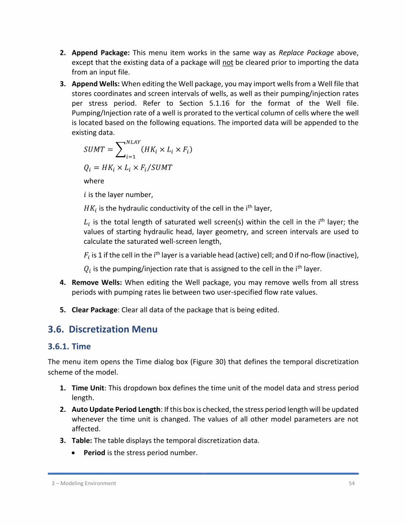
3 – Modeling Environment 54
2. Append Package: This menu item works in the same way as Replace Package above, except that the existing data of a package will not be cleared prior to importing the data from an input file.
3. Append Wells: When editing the Well package, you may import wells from a Well file that stores coordinates and screen intervals of wells, as well as their pumping/injection rates per stress period. Refer to Section 5.1.16 for the format of the Well file. Pumping/Injection rate of a well is prorated to the vertical column of cells where the well is located based on the following equations. The imported data will be appended to the existing data.
𝑆𝑈𝑀𝑇 = ∑ (𝐻𝐾𝑖 × 𝐿𝑖 × 𝐹𝑖)𝑁𝐿𝐴𝑌
𝑖=1
𝑄𝑖 = 𝐻𝐾𝑖 × 𝐿𝑖 × 𝐹𝑖 𝑆𝑈𝑀𝑇⁄
where
𝑖 is the layer number,
𝐻𝐾𝑖 is the hydraulic conductivity of the cell in the ith layer,
𝐿𝑖 is the total length of saturated well screen(s) within the cell in the ith layer; the values of starting hydraulic head, layer geometry, and screen intervals are used to calculate the saturated well-screen length,
𝐹𝑖 is 1 if the cell in the ith layer is a variable head (active) cell; and 0 if no-flow (inactive),
𝑄𝑖 is the pumping/injection rate that is assigned to the cell in the ith layer.
4. Remove Wells: When editing the Well package, you may remove wells from all stress periods with pumping rates lie between two user-specified flow rate values.
5. Clear Package: Clear all data of the package that is being edited.
3.6. Discretization Menu
3.6.1. Time
The menu item opens the Time dialog box (Figure 30) that defines the temporal discretization
scheme of the model.
1. Time Unit: This dropdown box defines the time unit of the model data and stress period length.
2. Auto Update Period Length: If this box is checked, the stress period length will be updated whenever the time unit is changed. The values of all other model parameters are not affected.
3. Table: The table displays the temporal discretization data.
• Period is the stress period number.
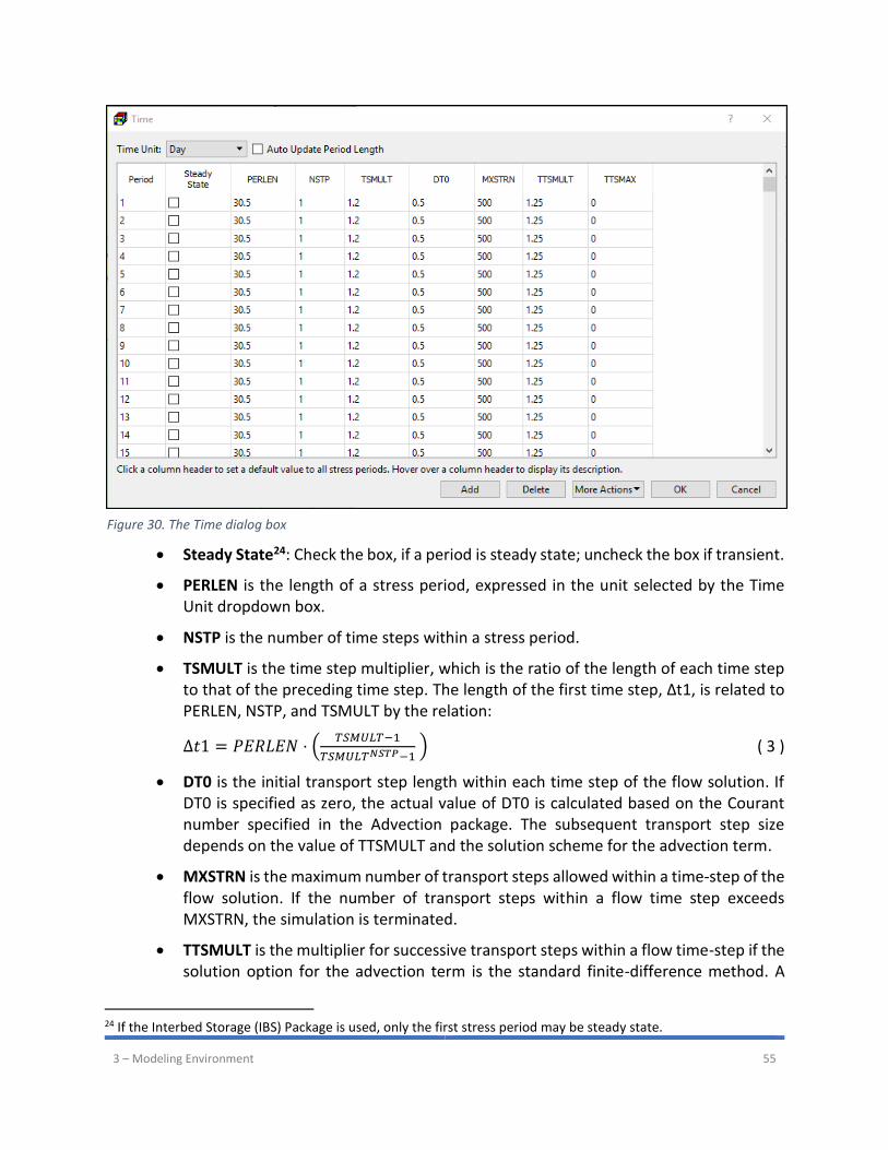
3 – Modeling Environment 55
• Steady State24: Check the box, if a period is steady state; uncheck the box if transient.
• PERLEN is the length of a stress period, expressed in the unit selected by the Time Unit dropdown box.
• NSTP is the number of time steps within a stress period.
• TSMULT is the time step multiplier, which is the ratio of the length of each time step to that of the preceding time step. The length of the first time step, Δt1, is related to PERLEN, NSTP, and TSMULT by the relation:
∆𝑡1 = 𝑃𝐸𝑅𝐿𝐸𝑁 ⋅ (𝑇𝑆𝑀𝑈𝐿𝑇−1
𝑇𝑆𝑀𝑈𝐿𝑇𝑁𝑆𝑇𝑃−1 ) ( 3 )
• DT0 is the initial transport step length within each time step of the flow solution. If DT0 is specified as zero, the actual value of DT0 is calculated based on the Courant number specified in the Advection package. The subsequent transport step size depends on the value of TTSMULT and the solution scheme for the advection term.
• MXSTRN is the maximum number of transport steps allowed within a time-step of the flow solution. If the number of transport steps within a flow time step exceeds MXSTRN, the simulation is terminated.
• TTSMULT is the multiplier for successive transport steps within a flow time-step if the solution option for the advection term is the standard finite-difference method. A
24 If the Interbed Storage (IBS) Package is used, only the first stress period may be steady state.
Figure 30. The Time dialog box
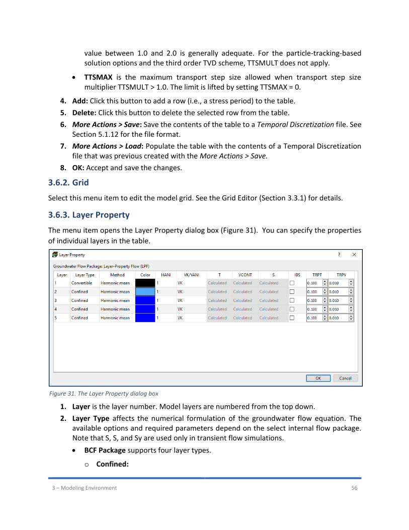
3 – Modeling Environment 56
value between 1.0 and 2.0 is generally adequate. For the particle-tracking-based solution options and the third order TVD scheme, TTSMULT does not apply.
• TTSMAX is the maximum transport step size allowed when transport step size multiplier TTSMULT > 1.0. The limit is lifted by setting TTSMAX = 0.
4. Add: Click this button to add a row (i.e., a stress period) to the table.
5. Delete: Click this button to delete the selected row from the table.
6. More Actions > Save: Save the contents of the table to a Temporal Discretization file. See Section 5.1.12 for the file format.
7. More Actions > Load: Populate the table with the contents of a Temporal Discretization file that was previous created with the More Actions > Save.
8. OK: Accept and save the changes.
3.6.2. Grid
Select this menu item to edit the model grid. See the Grid Editor (Section 3.3.1) for details.
3.6.3. Layer Property
The menu item opens the Layer Property dialog box (Figure 31). You can specify the properties
of individual layers in the table.
1. Layer is the layer number. Model layers are numbered from the top down.
2. Layer Type affects the numerical formulation of the groundwater flow equation. The available options and required parameters depend on the select internal flow package. Note that S, S, and Sy are used only in transient flow simulations.
• BCF Package supports four layer types.
o Confined:
Figure 31. The Layer Property dialog box
3 – Modeling Environment 57
Required input parameters: T and S
Interblock conductance is calculated based on input values of T, and therefore
remains unchanged for the entire simulation.
o Unconfined: The option is valid only for layer 1.
Required input parameters: HK and Sy.
Interblock conductance is calculated based on HK and saturated thickness that
may vary during a flow simulation.
o Limited Convertible between confined and unconfined.
Required input parameters: T, S, and Sy.
Interblock conductance is calculated based on input values of T, and therefore
remains constant for the entire simulation regardless of the saturated
thickness.
If the layer is fully saturated, the storage is calculated based on S; Otherwise Sy
and saturated thickness are used.
Vertical flow from above is limited if the layer desaturates.
o Full Convertible between confined and unconfined.
Required input parameters: HK, S, and Sy.
If the layer is not fully saturated, the storage is calculated based on Sy and the
saturated thickness; and the interblock conductance is calculated based on HK
and the saturated thickness.
If the layer is fully saturated, the storage is calculated based on S; and the
interblock conductance is calculated based on HK and the layer thickness.
Vertical flow from above is limited if the layer desaturates.
• LPF or UPW Package:
o Confined
Required input parameters: HK, Ss, and VK or VANI.
Interblock conductance is calculated based on HK and layer thickness, and
therefore remains constant for the entire simulation.
The storage is calculated based on Ss and layer thickness.
VK or VANI is used for calculating vertical conductance between layers.
o Convertible between confined and unconfined.
Required input parameters: HK, Ss, Sy, and VK or VANI.
If the layer is not fully saturated, the storage is calculated based on Sy and the
saturated thickness; and the interblock conductance is calculated based on HK
and the saturated thickness.
3 – Modeling Environment 58
If the layer is fully saturated, the storage is calculated based on Ss and the layer
thickness; and the interblock conductance is calculated based on HK and the
layer thickness.
VK or VANI is used for calculating vertical conductance between layers.
3. Method defines the method of calculating interblock transmissivity.
4. Color defines the color that is used to draw observation points and pathlines when they reside within the respective layer.
5. HANI defines the ratio of the HK along columns to HK along rows.
• BCF package:
o The absolute values of HANI are assigned to the TRPY array (i.e., an array
containing a horizontal anisotropic factor for each layer) in the BCF’s input file.
• LPF or UPW package:
o If HANI > 0, the specified HANI value is assigned to all cells in the layer.
o If HANI < 0, the values specified in Parameters > Horizontal Anisotropy are used
for the layer.
6. VK/VANI determines whether vertical hydraulic conductivity or vertical anisotropy is used for a layer.
• BCF package:
o This column is dimmed as input of VANI is not supported by BCF.
• LPF or UPW package:
o VK indicates that the values specified in Parameters > Vertical Hydraulic
Conductivity are used for the layer.
o VANI indicates that values specified in Parameters > Vertical Anisotropy (i.e., ratio
of horizontal to vertical hydraulic conductivity) are used for the layer.
7. T determines how transmissivity values are defined.
• BCF package requires transmissivity values for layers of the types Confined or Limited Convertible. To facilitate the data input, two options are available
o User-Specified: The values specified in Parameters > Transmissivity are used for
the layer.
o Calculated: The product of the layer thickness (i.e., layer top elevation – bottom
elevation) and the values specified in Parameter > Horizontal Hydraulic
Conductivity (i.e., HK) are used for the layer.
• LPF or UPW package:
o This column is dimmed as input of T is not supported.
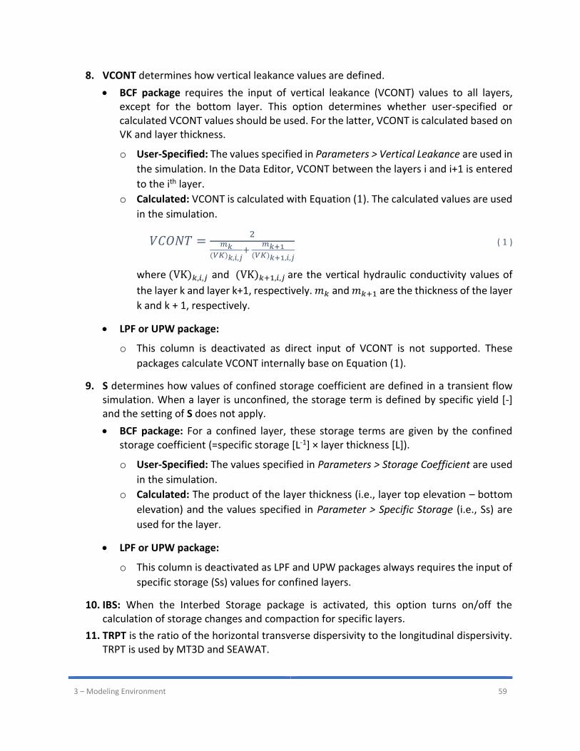
3 – Modeling Environment 59
8. VCONT determines how vertical leakance values are defined.
• BCF package requires the input of vertical leakance (VCONT) values to all layers, except for the bottom layer. This option determines whether user-specified or calculated VCONT values should be used. For the latter, VCONT is calculated based on VK and layer thickness.
o User-Specified: The values specified in Parameters > Vertical Leakance are used in
the simulation. In the Data Editor, VCONT between the layers i and i+1 is entered
to the ith layer.
o Calculated: VCONT is calculated with Equation (1). The calculated values are used
in the simulation.
𝑉𝐶𝑂𝑁𝑇 =2
𝑚𝑘(𝑉𝐾)𝑘,𝑖,𝑗
+ 𝑚𝑘+1
(𝑉𝐾)𝑘+1,𝑖,𝑗
( 1 )
where (VK)𝑘,𝑖,𝑗 and (VK)𝑘+1,𝑖,𝑗 are the vertical hydraulic conductivity values of
the layer k and layer k+1, respectively. 𝑚𝑘 and 𝑚𝑘+1 are the thickness of the layer
k and k + 1, respectively.
• LPF or UPW package:
o This column is deactivated as direct input of VCONT is not supported. These
packages calculate VCONT internally base on Equation (1).
9. S determines how values of confined storage coefficient are defined in a transient flow simulation. When a layer is unconfined, the storage term is defined by specific yield [-] and the setting of S does not apply.
• BCF package: For a confined layer, these storage terms are given by the confined storage coefficient (=specific storage [L-1] × layer thickness [L]).
o User-Specified: The values specified in Parameters > Storage Coefficient are used
in the simulation.
o Calculated: The product of the layer thickness (i.e., layer top elevation – bottom
elevation) and the values specified in Parameter > Specific Storage (i.e., Ss) are
used for the layer.
• LPF or UPW package:
o This column is deactivated as LPF and UPW packages always requires the input of
specific storage (Ss) values for confined layers.
10. IBS: When the Interbed Storage package is activated, this option turns on/off the calculation of storage changes and compaction for specific layers.
11. TRPT is the ratio of the horizontal transverse dispersivity to the longitudinal dispersivity. TRPT is used by MT3D and SEAWAT.
3 – Modeling Environment 60
12. TRPV is the ratio of the vertical transverse dispersivity to the longitudinal dispersivity. TRPV is used by MT3D and SEAWAT.
3.6.4. Layer Top Elevation and Layer Bottom Elevation
Select Discretization > Layer Top Elevation or Discretization > Layer Bottom Elevation to define,
respectively, the top or bottom elevations of the model cells with the Data Editor.
3.6.5. IBOUND (Flow)
MODFLOW requires an IBOUND array, which contains a value for each model cell. A positive value
in the IBOUND array defines a variable-head (i.e., active) cell where the hydraulic head is
computed, a negative value defines a constant head cell and the value 0 defines a no-flow cell
(i.e., inactive) cell. It is suggested to use 1 for variable-head cells, 0 for no-flow cells and -1 for
constant head cells. Flux boundaries may be simulated by assigning appropriate fluxes with the
Flow and Head Boundary or the Well package.
For constant head cells, the hydraulic head is hold at the starting value throughout the
simulation. The starting hydraulic head is specified in Parameters > Starting and Prescribed
Hydraulic Heads. A constant head boundary exists when an aquifer is in direct hydraulic contact
with a river, a lake, or a reservoir in which the water (groundwater) level is known to be constant.
It is important to know that constant head boundaries can provide inexhaustible supply or sink
of water. Care must be taken when using constant head boundaries, as a groundwater system
may get or lose unrealistically much water as necessary from or to such a boundary. It is
recommended to avoid using this boundary condition on the upstream side of the groundwater
flow direction. Consider using the General-Head Boundary or the Time-Variant Specified-Head
packages, if the hydraulic head at the constant head boundary varies with time. Head-dependent
boundary conditions may be simulated by means of the general head boundary, river, stream,
reservoir or drain package.
3.6.6. ICBUND (Transport)
The transport models MT3D and SEAWAT require an ICBUND array, which contains a value for
each model cell. A positive value in the ICBUND array defines an active concentration cell (the
concentration varies with time and is calculated), a negative value defines a constant-
concentration cell (the concentration is constant) and the value 0 defines an inactive
concentration cell (no transport simulation takes place at such cells). It is recommended to use
the value 1 for an active concentration cell, -1 for a constant-concentration cell, and 0 for an
inactive concentration cell. Note that the ICBUND array applies to all species. Other types of
boundary conditions are implemented by assigning concentrations to inflows or assigning a mass-
loading rate to cells. For details, see Section 3.8.3.3.4.
No-flow or dry cells are automatically converted to inactive concentration cells. Variable-head
cells may be treated as inactive concentration cells to minimize the area needed for transport
3 – Modeling Environment 61
simulation, if the solute transport is insignificant near those cells. For constant-concentration
cells, the initial concentration remains the same at the cell throughout the simulation. A constant
head cell may or may not be a constant-concentration cell. The initial concentration is specified
in Models > Transport (MT3D/SEAWAT) > Initial Concentration.
3.7. Parameters Menu
3.7.1. Starting Hydraulic Head
MODFLOW requires a starting hydraulic head value (starting head) for each model cell at the
beginning of a flow simulation. Starting heads at constant head cells are used as prescribed head
values and remain constant throughout the flow simulation.
For steady-state flow simulations, the starting heads are used as initial values for the iterative
equation solvers and should be set as close as possible to the final head solution. For an
unconfined or a convertible layer, the starting head of a constant head cell must be higher than
the elevation of the cell bottom. Otherwise, MODFLOW will write the message CONSTANT-HEAD
CELL WENT DRY – SIMULATION ABORTED to its run listing file and then abort the simulation.
In a transient flow simulation, the starting heads provide a reference elevations for the solution.
It is a standard practice to use heads generated by a steady-state model as the initial conditions
for a transient model, see Section 7.4 of (Anderson, et al., 2015) for more details.
3.7.2. Horizontal Hydraulic Conductivity (HK) and Transmissivity (T)
HK is the horizontal hydraulic conductivity along model rows. T is the product of HK and layer
thickness. Typical values and ranges of HK for diverse types of soils are given in many
groundwater textbooks, for example (Freeze, et al., 1979), (Spitz, et al., 1996) and (Fetter, 1994).
If the BCF package is selected as the internal flow package, HK is required for unconfined and full
convertible layers and T is required for confined or limited convertible layers. You have the option
to enter T directly by selecting Parameters > Transmissivity, or enter HK by selecting Parameters
> Horizontal Hydraulic Conductivity and let PM calculate T by using the layer thickness and HK.
See Section 3.6.3 for details.
If the LPF or UPW package is selected as the internal flow package, HK is required for all layer
types and direct input of T is not possible.
3.7.3. Horizontal Anisotropy (HANI)
HANI is the ratio of horizontal hydraulic conductivity along columns to horizontal hydraulic
conductivity along rows.
If the BCF package is selected as the internal flow package, this menu item is deactivated as the
BCF only supports the input of layer-by-later HANI values and does not support the cell-by-cell
3 – Modeling Environment 62
HANI values. Use the Layer Property dialog box (Section 3.6.3) to input the layer-by-layer HANI
values.
If the LPF or UPW package is selected as the internal flow package, you may use this menu item
to enter the cell-by-cell HANI values. The entered values may or may not be used in a simulation,
depending on the settings of the HANI column in the Layer Property dialog box. See Section 3.6.3
for details.
3.7.4. Vertical Hydraulic Conductivity (VK) and Vertical Leakance (VCONT)
The vertical leakance between two vertically adjacent cells is calculated based on Equation (1).
The VCONT value is multiplied by cell area to obtain vertical conductance, which is used for
formulating the vertical flow term by MODFLOW.
If the BCF package is selected as the internal flow package, an array of VCONT values is required
for each layer, except for the bottom layer. You have the option to enter VCONT directly by
selecting Parameters > Vertical Leakance, or enter VK by selecting Parameters > Vertical
Hydraulic Conductivity and let PM calculate VCONT. See the setting of VCONT in Section 3.6.3 for
details.
If the LPF or UPW package is selected as the internal flow package, VCONT is calculated for all
layer types by LPF or UPW internally. The calculation is based on VK or Vertical Anisotropy. A
direct input of VCONT is not possible.
3.7.5. Vertical Anisotropy (VANI)
VANI is the ratio of HK to VK.
If the BCF package is selected as the internal flow package, this menu item is deactivated as the
input of VANI is not supported.
If the LPF or UPW package is selected as the internal flow package, you have the option to enter
VK directly by selecting Parameters > Vertical Hydraulic Conductivity or enter VANI and let PM
determine VK (= HK/VANI).
3.7.6. Specific Storage (Ss) and Storage Coefficient (S)
For a steady state simulation, these menu items are not used and are deactivated. S is required
by MODFLOW for confined or convertible layers.
Specific storage or specific storativity is defined as the volume fraction of water that a unit column
of aquifer releases from storage under a unit decline in hydraulic head. The specific storage is a
function of the compressibility of the water and the elastic property of the soil matrix and ranges
in value from 3.3 × 10⁻⁶ [m-1] of rock to 2.0 × 10⁻²
[m-1] of plastic clay (Domenico, 1972).
3 – Modeling Environment 63
In a confined layer, the storage term is given by the storativity or storage coefficient (= specific
storage [L-1] × layer thickness [L]). The storativity is sometimes referred to as confined storage
coefficient.
If the BCF package is selected as the internal flow package, you have the option to enter S directly
by selecting Parameters > Storage Coefficient, or enter Ss by selecting Parameters > Specific
Storage and let PM calculate S. See the setting of S in Section 3.6.3 for details.
If the LPF or UPW package is selected as the internal flow package, Ss is required. A direct input
of S is not possible.
3.7.7. Specific Yield (Sy)
For a steady state simulation, this menu item is not used and is deactivated. Sy is required by
MODFLOW for unconfined or convertible layers.
Specific yield is defined as the volume of water that an unconfined aquifer releases from storage
per unit surface area of aquifer per unit decline in the water table. Specific yield is a function of
porosity (and is not necessarily equal to porosity), because a certain amount of water is held in
the soil matrix and cannot be removed by gravity drainage. Refer to (Spitz, et al., 1996) for a
summary of values of specific yield. Refer to (Bear, 1972), (Bear, 1979) or (Freeze, et al., 1979)
for detailed explanation of storage terms and their definitions.
3.7.8. Effective Porosity (ne)
Effective porosity is used by MODPATH, MT3D and SEAWAT for calculating the average velocity
of the flow through the porous medium.
If the total unit volume V of a soil matrix is divided into the volume of the solid portion Vs and the
volume of voids Vv, the total porosity n is defined as n = Vv/V. Effective porosity (with the respect
to flow through the medium) is always less than total porosity, sometimes (as in the case of clays)
much less, because some of the pore spaces may be too small or too poorly connected so that
part of the fluid is immobile or partially immobile. A summary of representative porosity values
for different soil types can be found in (Zheng, et al., 1995) or (Domenico, et al., 1997).
3.7.9. Stop Zone
Stop Zone is used by MODPATH to define stopping locations for particles. The Stop Zone option
of MODPATH is activated by specifying a positive Stop Zone value to MODPATH’s settings window
(Figure 117). Particles stop, when they enter cells with the specified Stop Zone value.
3.7.10. Retardation Factor (R)
Retardation factor is used by MODPATH as a scaling factor for the magnitude of the velocity.
3 – Modeling Environment 64
The retardation factor is a function of the porosity, the density of the geologic material, and the
sorption coefficient. A detailed discussion of the retardation factor can be found in (Domenico, et al.,
1997). The effect of linear sorption on the apparent velocity of a reactive solute can be examined
using the particle-tracking method in MODPATH by dividing the velocity components by a retardation
factor. For nonreactive solutes that do not interact with the surrounding rock, the retardation factor
is equal to 1 and the magnitude of the apparent solute velocity is equal to that of the groundwater
velocity. For solutes affected by linear sorption, the retardation factor is greater than 1 and the
magnitude of the apparent solute velocity is less than that of the groundwater velocity.
3.7.11. Bulk Density
The cell-by-cell bulk density data are used by the Reaction package of MT3D and SEAWAT for
simulating sorption effects.
3.7.12. Static Sandboxes
A Static Sandbox is a place where you can store data for visualization purposes. The values
specified in a Static Sandbox do not vary with time and will not be used in simulation.
3.7.13. Transient Sandboxes
A Transient Sandbox is a place where you can store time-dependent data for animation and
visualization purposes. For a model with multiple stress periods, the user may assign various
matrix values to (the end of the selected) stress periods. If a contour map is created with the data
of transient sandbox, the contour map will transit between stress periods based on the linearly
interpolated matrix values of those stress periods.
3.8. Models Menu
3.8.1. MODFLOW
3.8.1.1. Packages
To activate a package and edit its data, select the respective item. If the package is already
activated, you will have the opportunity to edit its data or deactivate the package.
Drain (DRN)
The Drain (DRN) Package is used to simulate effects of features such as agricultural drains, which
remove groundwater from aquifer at a rate proportional to the head difference between the
aquifer and the drain. For a model cell containing a drain, the recharge rate from the drain to the
cell is always zero, and the discharge rate from the cell to the drain is calculated by
𝑄𝑑 = 𝐶𝑑 ⋅ (ℎ − ℎ𝑑) if h > hd ( 2 )
𝑄𝑑 = 0 if h <= hd ( 3 )
where
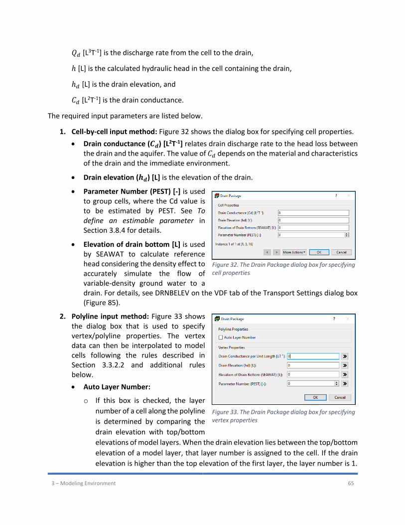
3 – Modeling Environment 65
𝑄𝑑 [L3T-1] is the discharge rate from the cell to the drain,
ℎ [L] is the calculated hydraulic head in the cell containing the drain,
ℎ𝑑 [L] is the drain elevation, and
𝐶𝑑 [L2T-1] is the drain conductance.
The required input parameters are listed below.
1. Cell-by-cell input method: Figure 32 shows the dialog box for specifying cell properties.
• Drain conductance (𝑪𝒅) [L2T-1] relates drain discharge rate to the head loss between the drain and the aquifer. The value of 𝐶𝑑 depends on the material and characteristics of the drain and the immediate environment.
• Drain elevation (𝒉𝒅) [L] is the elevation of the drain.
• Parameter Number (PEST) [-] is used to group cells, where the Cd value is to be estimated by PEST. See To define an estimable parameter in Section 3.8.4 for details.
• Elevation of drain bottom [L] is used by SEAWAT to calculate reference head considering the density effect to accurately simulate the flow of variable-density ground water to a drain. For details, see DRNBELEV on the VDF tab of the Transport Settings dialog box (Figure 85).
2. Polyline input method: Figure 33 shows the dialog box that is used to specify vertex/polyline properties. The vertex data can then be interpolated to model cells following the rules described in Section 3.3.2.2 and additional rules below.
• Auto Layer Number:
o If this box is checked, the layer
number of a cell along the polyline
is determined by comparing the
drain elevation with top/bottom
elevations of model layers. When the drain elevation lies between the top/bottom
elevation of a model layer, that layer number is assigned to the cell. If the drain
elevation is higher than the top elevation of the first layer, the layer number is 1.
Figure 32. The Drain Package dialog box for specifying cell properties
Figure 33. The Drain Package dialog box for specifying vertex properties
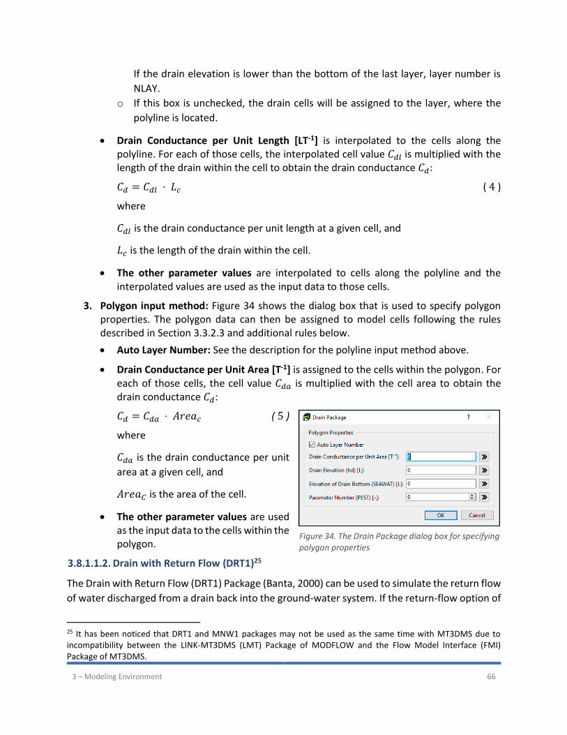
3 – Modeling Environment 66
If the drain elevation is lower than the bottom of the last layer, layer number is
NLAY.
o If this box is unchecked, the drain cells will be assigned to the layer, where the
polyline is located.
• Drain Conductance per Unit Length [LT-1] is interpolated to the cells along the polyline. For each of those cells, the interpolated cell value 𝐶𝑑𝑙 is multiplied with the length of the drain within the cell to obtain the drain conductance 𝐶𝑑:
𝐶𝑑 = 𝐶𝑑𝑙 ⋅ 𝐿𝑐 ( 4 )
where
𝐶𝑑𝑙 is the drain conductance per unit length at a given cell, and
𝐿𝑐 is the length of the drain within the cell.
• The other parameter values are interpolated to cells along the polyline and the interpolated values are used as the input data to those cells.
3. Polygon input method: Figure 34 shows the dialog box that is used to specify polygon properties. The polygon data can then be assigned to model cells following the rules described in Section 3.3.2.3 and additional rules below.
• Auto Layer Number: See the description for the polyline input method above.
• Drain Conductance per Unit Area [T-1] is assigned to the cells within the polygon. For each of those cells, the cell value 𝐶𝑑𝑎 is multiplied with the cell area to obtain the drain conductance 𝐶𝑑:
𝐶𝑑 = 𝐶𝑑𝑎 ⋅ 𝐴𝑟𝑒𝑎𝑐 ( 5 )
where
𝐶𝑑𝑎 is the drain conductance per unit
area at a given cell, and
𝐴𝑟𝑒𝑎𝐶 is the area of the cell.
• The other parameter values are used as the input data to the cells within the polygon.
Drain with Return Flow (DRT1)25
The Drain with Return Flow (DRT1) Package (Banta, 2000) can be used to simulate the return flow
of water discharged from a drain back into the ground-water system. If the return-flow option of
25 It has been noticed that DRT1 and MNW1 packages may not be used as the same time with MT3DMS due to incompatibility between the LINK-MT3DMS (LMT) Package of MODFLOW and the Flow Model Interface (FMI) Package of MT3DMS.
Figure 34. The Drain Package dialog box for specifying polygon properties
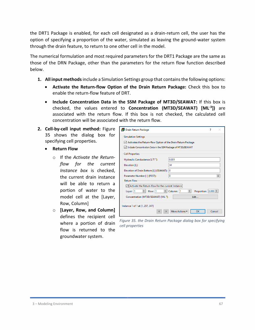
3 – Modeling Environment 67
the DRT1 Package is enabled, for each cell designated as a drain-return cell, the user has the
option of specifying a proportion of the water, simulated as leaving the ground-water system
through the drain feature, to return to one other cell in the model.
The numerical formulation and most required parameters for the DRT1 Package are the same as
those of the DRN Package, other than the parameters for the return flow function described
below.
1. All input methods include a Simulation Settings group that contains the following options:
• Activate the Return-flow Option of the Drain Return Package: Check this box to enable the return-flow feature of DRT.
• Include Concentration Data in the SSM Package of MT3D/SEAWAT: If this box is checked, the values entered to Concentration (MT3D/SEAWAT) [ML-3]) are associated with the return flow. If this box is not checked, the calculated cell concentration will be associated with the return flow.
2. Cell-by-cell input method: Figure 35 shows the dialog box for specifying cell properties.
• Return Flow
o If the Activate the Return-
flow for the current
Instance box is checked,
the current drain instance
will be able to return a
portion of water to the
model cell at the [Layer,
Row, Column]
o [Layer, Row, and Column]
defines the recipient cell
where a portion of drain
flow is returned to the
groundwater system.
Figure 35. the Drain Return Package dialog box for specifying cell properties
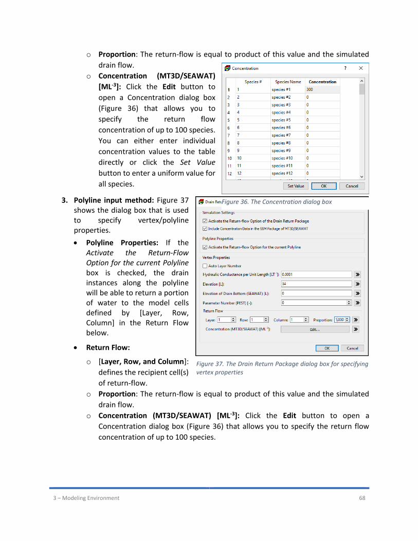
3 – Modeling Environment 68
o Proportion: The return-flow is equal to product of this value and the simulated
drain flow.
o Concentration (MT3D/SEAWAT)
[ML-3]: Click the Edit button to
open a Concentration dialog box
(Figure 36) that allows you to
specify the return flow
concentration of up to 100 species.
You can either enter individual
concentration values to the table
directly or click the Set Value
button to enter a uniform value for
all species.
3. Polyline input method: Figure 37 shows the dialog box that is used to specify vertex/polyline properties.
• Polyline Properties: If the Activate the Return-Flow Option for the current Polyline box is checked, the drain instances along the polyline will be able to return a portion of water to the model cells defined by [Layer, Row, Column] in the Return Flow below.
• Return Flow:
o [Layer, Row, and Column]:
defines the recipient cell(s)
of return-flow.
o Proportion: The return-flow is equal to product of this value and the simulated
drain flow.
o Concentration (MT3D/SEAWAT) [ML-3]: Click the Edit button to open a
Concentration dialog box (Figure 36) that allows you to specify the return flow
concentration of up to 100 species.
Figure 37. The Drain Return Package dialog box for specifying vertex properties
Figure 36. The Concentration dialog box
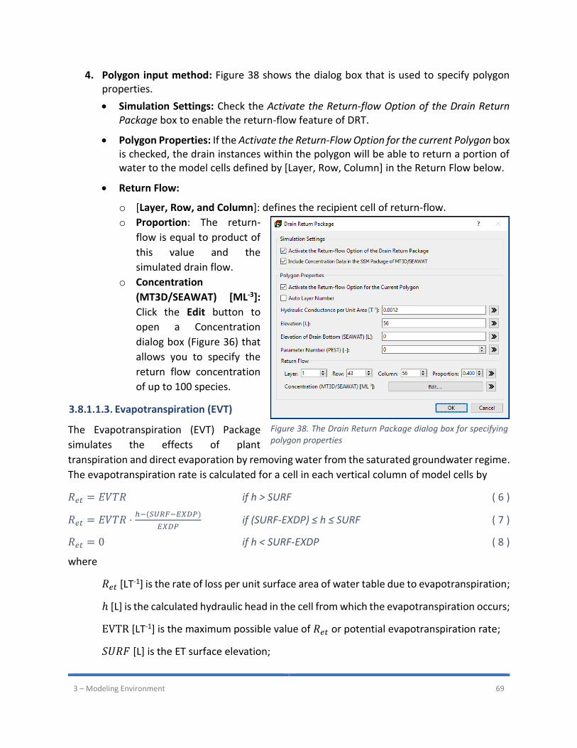
3 – Modeling Environment 69
4. Polygon input method: Figure 38 shows the dialog box that is used to specify polygon properties.
• Simulation Settings: Check the Activate the Return-flow Option of the Drain Return Package box to enable the return-flow feature of DRT.
• Polygon Properties: If the Activate the Return-Flow Option for the current Polygon box is checked, the drain instances within the polygon will be able to return a portion of water to the model cells defined by [Layer, Row, Column] in the Return Flow below.
• Return Flow:
o [Layer, Row, and Column]: defines the recipient cell of return-flow.
o Proportion: The return-
flow is equal to product of
this value and the
simulated drain flow.
o Concentration
(MT3D/SEAWAT) [ML-3]:
Click the Edit button to
open a Concentration
dialog box (Figure 36) that
allows you to specify the
return flow concentration
of up to 100 species.
Evapotranspiration (EVT)
The Evapotranspiration (EVT) Package
simulates the effects of plant
transpiration and direct evaporation by removing water from the saturated groundwater regime.
The evapotranspiration rate is calculated for a cell in each vertical column of model cells by
𝑅𝑒𝑡 = 𝐸𝑉𝑇𝑅 if h > SURF ( 6 )
𝑅𝑒𝑡 = 𝐸𝑉𝑇𝑅 ⋅ℎ−(𝑆𝑈𝑅𝐹−𝐸𝑋𝐷𝑃)
𝐸𝑋𝐷𝑃 if (SURF-EXDP) ≤ h ≤ SURF ( 7 )
𝑅𝑒𝑡 = 0 if h < SURF-EXDP ( 8 )
where
𝑅𝑒𝑡 [LT-1] is the rate of loss per unit surface area of water table due to evapotranspiration;
ℎ [L] is the calculated hydraulic head in the cell from which the evapotranspiration occurs;
EVTR [LT-1] is the maximum possible value of 𝑅𝑒𝑡 or potential evapotranspiration rate;
𝑆𝑈𝑅𝐹 [L] is the ET surface elevation;
Figure 38. The Drain Return Package dialog box for specifying polygon properties
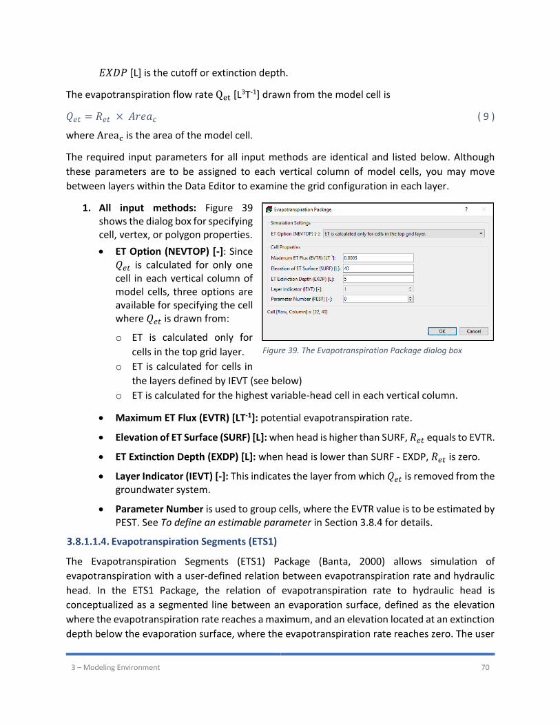
3 – Modeling Environment 70
𝐸𝑋𝐷𝑃 [L] is the cutoff or extinction depth.
The evapotranspiration flow rate Qet [L3T-1] drawn from the model cell is
𝑄𝑒𝑡 = 𝑅𝑒𝑡 × 𝐴𝑟𝑒𝑎𝑐 ( 9 )
where Areac is the area of the model cell.
The required input parameters for all input methods are identical and listed below. Although
these parameters are to be assigned to each vertical column of model cells, you may move
between layers within the Data Editor to examine the grid configuration in each layer.
1. All input methods: Figure 39 shows the dialog box for specifying cell, vertex, or polygon properties.
• ET Option (NEVTOP) [-]: Since 𝑄𝑒𝑡 is calculated for only one cell in each vertical column of model cells, three options are available for specifying the cell where 𝑄𝑒𝑡 is drawn from:
o ET is calculated only for
cells in the top grid layer.
o ET is calculated for cells in
the layers defined by IEVT (see below)
o ET is calculated for the highest variable-head cell in each vertical column.
• Maximum ET Flux (EVTR) [LT-1]: potential evapotranspiration rate.
• Elevation of ET Surface (SURF) [L]: when head is higher than SURF, 𝑅𝑒𝑡 equals to EVTR.
• ET Extinction Depth (EXDP) [L]: when head is lower than SURF - EXDP, 𝑅𝑒𝑡 is zero.
• Layer Indicator (IEVT) [-]: This indicates the layer from which 𝑄𝑒𝑡 is removed from the groundwater system.
• Parameter Number is used to group cells, where the EVTR value is to be estimated by PEST. See To define an estimable parameter in Section 3.8.4 for details.
Evapotranspiration Segments (ETS1)
The Evapotranspiration Segments (ETS1) Package (Banta, 2000) allows simulation of
evapotranspiration with a user-defined relation between evapotranspiration rate and hydraulic
head. In the ETS1 Package, the relation of evapotranspiration rate to hydraulic head is
conceptualized as a segmented line between an evaporation surface, defined as the elevation
where the evapotranspiration rate reaches a maximum, and an elevation located at an extinction
depth below the evaporation surface, where the evapotranspiration rate reaches zero. The user
Figure 39. The Evapotranspiration Package dialog box
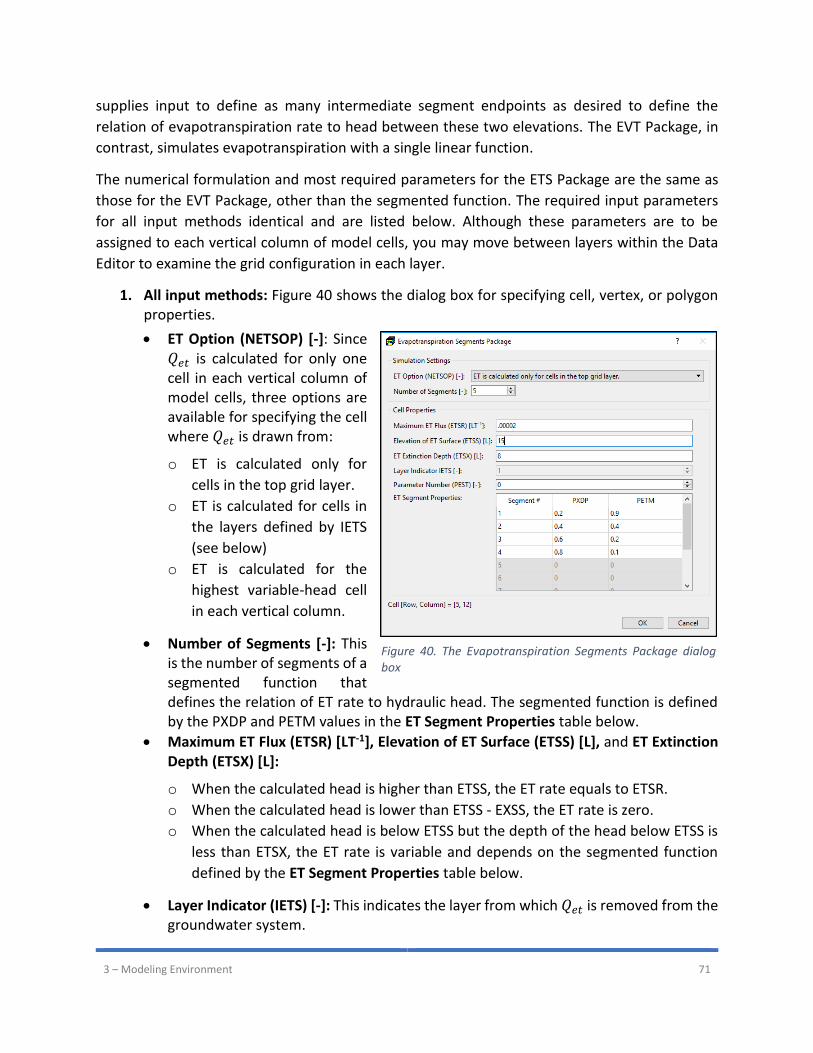
3 – Modeling Environment 71
supplies input to define as many intermediate segment endpoints as desired to define the
relation of evapotranspiration rate to head between these two elevations. The EVT Package, in
contrast, simulates evapotranspiration with a single linear function.
The numerical formulation and most required parameters for the ETS Package are the same as
those for the EVT Package, other than the segmented function. The required input parameters
for all input methods identical and are listed below. Although these parameters are to be
assigned to each vertical column of model cells, you may move between layers within the Data
Editor to examine the grid configuration in each layer.
1. All input methods: Figure 40 shows the dialog box for specifying cell, vertex, or polygon properties.
• ET Option (NETSOP) [-]: Since 𝑄𝑒𝑡 is calculated for only one cell in each vertical column of model cells, three options are available for specifying the cell where 𝑄𝑒𝑡 is drawn from:
o ET is calculated only for
cells in the top grid layer.
o ET is calculated for cells in
the layers defined by IETS
(see below)
o ET is calculated for the
highest variable-head cell
in each vertical column.
• Number of Segments [-]: This is the number of segments of a segmented function that defines the relation of ET rate to hydraulic head. The segmented function is defined by the PXDP and PETM values in the ET Segment Properties table below.
• Maximum ET Flux (ETSR) [LT-1], Elevation of ET Surface (ETSS) [L], and ET Extinction Depth (ETSX) [L]:
o When the calculated head is higher than ETSS, the ET rate equals to ETSR.
o When the calculated head is lower than ETSS - EXSS, the ET rate is zero.
o When the calculated head is below ETSS but the depth of the head below ETSS is
less than ETSX, the ET rate is variable and depends on the segmented function
defined by the ET Segment Properties table below.
• Layer Indicator (IETS) [-]: This indicates the layer from which 𝑄𝑒𝑡 is removed from the groundwater system.
Figure 40. The Evapotranspiration Segments Package dialog box
3 – Modeling Environment 72
• Parameter Number is used to group cells, where the ETSR value is to be estimated by PEST. See To define an estimable parameter in Section 3.8.4 for details.
• ET Segment Properties:
o PXDP is a proportion of the extinction depth (dimensionless), measured
downward from the ET surface, which, with PETM, defines the shape of the
relation between the evapotranspiration rate and head. PXDP is 0.0 at the ET
surface and is 1.0 at the extinction depth. Repetitions of PXDP and PETM are to be
specified in sequence such that the first occurrence represents the bottom of the
first segment, and subsequent repetitions represent the bottom of successively
lower segments. Accordingly, PXDP values for later repetitions (representing
lower segments) should be greater than PXDP values for earlier repetitions.
o PETM is a proportion of the maximum evapotranspiration rate (dimensionless)
which, with PXDP, defines the shape of the relation between the
evapotranspiration rate and head. PETM is 1.0 at the ET surface and is 0.0 at the
extinction depth. Repetitions of PXDP and PETM are to be specified in sequence
such that the first occurrence represents the bottom of the first segment, and
subsequent repetitions represent the bottoms of successively lower segments.
Accordingly, PETM values for later repetitions (representing lower segments)
generally would be less than PETM values for earlier repetitions.
Flow and Head Boundary (FHB1)
The Flow and Head Boundary (FHB1) Package (Leake, et al., 1997) allows you to specify flow or
head boundary conditions that vary at times other than starting and ending times of stress
periods and associated time steps. Values of flow and (or) head at each time step are calculated
by linear interpolation of user-specified time-series values. First, an array of simulation times is
defined, and then for each FHB1 cell instance, the flow or head values are assigned to each of
those simulation times. The ability to assign variable flow and head conditions defined at times
not corresponding with the model stress periods allows greater flexibility in simulating natural
geohydrologic systems and, at the same time, improves the efficiency of the methods used to
represent these systems.
The FHB1 Package can be used as an alternative and/or supplement to using the Well (WEL)
Package or the Recharge (RCH) Package for simulating specified-flow boundaries. FHB1 also is an
alternative and/or supplement to the Time-Variant Specified-Head (CHD) Package for simulating
specified-head boundaries.
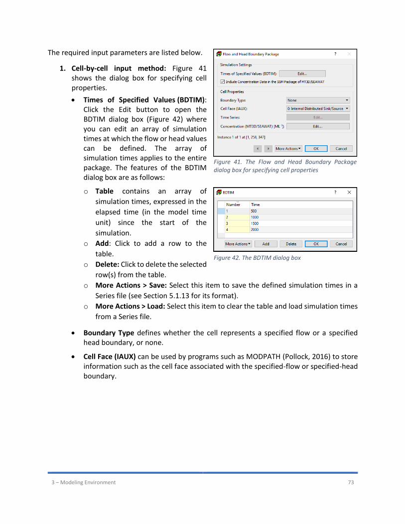
3 – Modeling Environment 73
The required input parameters are listed below.
1. Cell-by-cell input method: Figure 41 shows the dialog box for specifying cell properties.
• Times of Specified Values (BDTIM): Click the Edit button to open the BDTIM dialog box (Figure 42) where you can edit an array of simulation times at which the flow or head values can be defined. The array of simulation times applies to the entire package. The features of the BDTIM dialog box are as follows:
o Table contains an array of
simulation times, expressed in the
elapsed time (in the model time
unit) since the start of the
simulation.
o Add: Click to add a row to the
table.
o Delete: Click to delete the selected
row(s) from the table.
o More Actions > Save: Select this item to save the defined simulation times in a
Series file (see Section 5.1.13 for its format).
o More Actions > Load: Select this item to clear the table and load simulation times
from a Series file.
• Boundary Type defines whether the cell represents a specified flow or a specified head boundary, or none.
• Cell Face (IAUX) can be used by programs such as MODPATH (Pollock, 2016) to store information such as the cell face associated with the specified-flow or specified-head boundary.
Figure 42. The BDTIM dialog box
Figure 41. The Flow and Head Boundary Package dialog box for specifying cell properties
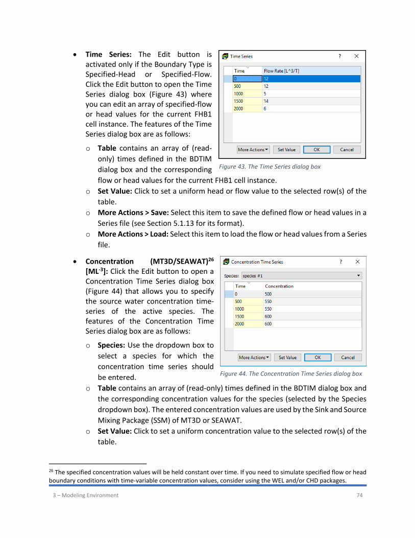
3 – Modeling Environment 74
• Time Series: The Edit button is activated only if the Boundary Type is Specified-Head or Specified-Flow. Click the Edit button to open the Time Series dialog box (Figure 43) where you can edit an array of specified-flow or head values for the current FHB1 cell instance. The features of the Time Series dialog box are as follows:
o Table contains an array of (read-
only) times defined in the BDTIM
dialog box and the corresponding
flow or head values for the current FHB1 cell instance.
o Set Value: Click to set a uniform head or flow value to the selected row(s) of the
table.
o More Actions > Save: Select this item to save the defined flow or head values in a
Series file (see Section 5.1.13 for its format).
o More Actions > Load: Select this item to load the flow or head values from a Series
file.
• Concentration (MT3D/SEAWAT)26 [ML-3]: Click the Edit button to open a Concentration Time Series dialog box (Figure 44) that allows you to specify the source water concentration time-series of the active species. The features of the Concentration Time Series dialog box are as follows:
o Species: Use the dropdown box to
select a species for which the
concentration time series should
be entered.
o Table contains an array of (read-only) times defined in the BDTIM dialog box and
the corresponding concentration values for the species (selected by the Species
dropdown box). The entered concentration values are used by the Sink and Source
Mixing Package (SSM) of MT3D or SEAWAT.
o Set Value: Click to set a uniform concentration value to the selected row(s) of the
table.
26 The specified concentration values will be held constant over time. If you need to simulate specified flow or head boundary conditions with time-variable concentration values, consider using the WEL and/or CHD packages.
Figure 43. The Time Series dialog box
Figure 44. The Concentration Time Series dialog box
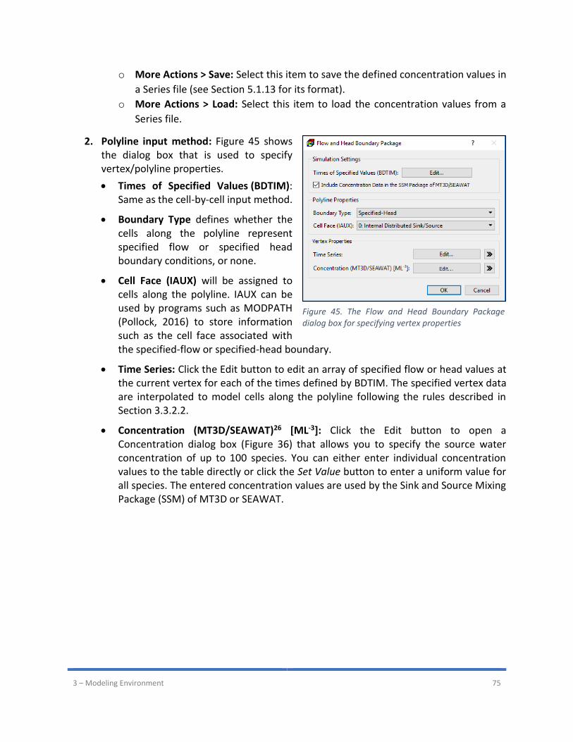
3 – Modeling Environment 75
o More Actions > Save: Select this item to save the defined concentration values in
a Series file (see Section 5.1.13 for its format).
o More Actions > Load: Select this item to load the concentration values from a
Series file.
2. Polyline input method: Figure 45 shows the dialog box that is used to specify vertex/polyline properties.
• Times of Specified Values (BDTIM): Same as the cell-by-cell input method.
• Boundary Type defines whether the cells along the polyline represent specified flow or specified head boundary conditions, or none.
• Cell Face (IAUX) will be assigned to cells along the polyline. IAUX can be used by programs such as MODPATH (Pollock, 2016) to store information such as the cell face associated with the specified-flow or specified-head boundary.
• Time Series: Click the Edit button to edit an array of specified flow or head values at the current vertex for each of the times defined by BDTIM. The specified vertex data are interpolated to model cells along the polyline following the rules described in Section 3.3.2.2.
• Concentration (MT3D/SEAWAT)26 [ML-3]: Click the Edit button to open a Concentration dialog box (Figure 36) that allows you to specify the source water concentration of up to 100 species. You can either enter individual concentration values to the table directly or click the Set Value button to enter a uniform value for all species. The entered concentration values are used by the Sink and Source Mixing Package (SSM) of MT3D or SEAWAT.
Figure 45. The Flow and Head Boundary Package dialog box for specifying vertex properties
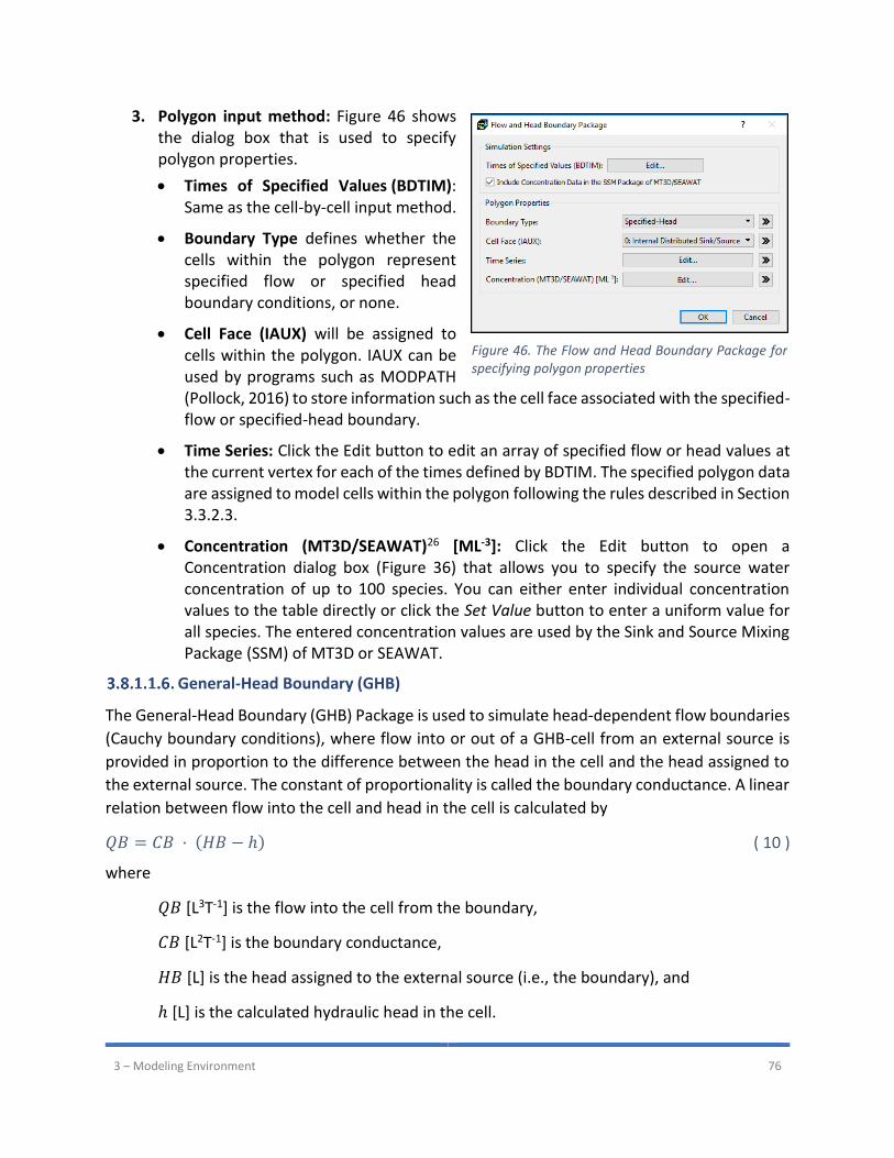
3 – Modeling Environment 76
3. Polygon input method: Figure 46 shows the dialog box that is used to specify polygon properties.
• Times of Specified Values (BDTIM): Same as the cell-by-cell input method.
• Boundary Type defines whether the cells within the polygon represent specified flow or specified head boundary conditions, or none.
• Cell Face (IAUX) will be assigned to cells within the polygon. IAUX can be used by programs such as MODPATH (Pollock, 2016) to store information such as the cell face associated with the specified-flow or specified-head boundary.
• Time Series: Click the Edit button to edit an array of specified flow or head values at the current vertex for each of the times defined by BDTIM. The specified polygon data are assigned to model cells within the polygon following the rules described in Section 3.3.2.3.
• Concentration (MT3D/SEAWAT)26 [ML-3]: Click the Edit button to open a Concentration dialog box (Figure 36) that allows you to specify the source water concentration of up to 100 species. You can either enter individual concentration values to the table directly or click the Set Value button to enter a uniform value for all species. The entered concentration values are used by the Sink and Source Mixing Package (SSM) of MT3D or SEAWAT.
General-Head Boundary (GHB)
The General-Head Boundary (GHB) Package is used to simulate head-dependent flow boundaries
(Cauchy boundary conditions), where flow into or out of a GHB-cell from an external source is
provided in proportion to the difference between the head in the cell and the head assigned to
the external source. The constant of proportionality is called the boundary conductance. A linear
relation between flow into the cell and head in the cell is calculated by
𝑄𝐵 = 𝐶𝐵 ⋅ (𝐻𝐵 − ℎ) ( 10 )
where
𝑄𝐵 [L3T-1] is the flow into the cell from the boundary,
𝐶𝐵 [L2T-1] is the boundary conductance,
𝐻𝐵 [L] is the head assigned to the external source (i.e., the boundary), and
ℎ [L] is the calculated hydraulic head in the cell.
Figure 46. The Flow and Head Boundary Package for specifying polygon properties
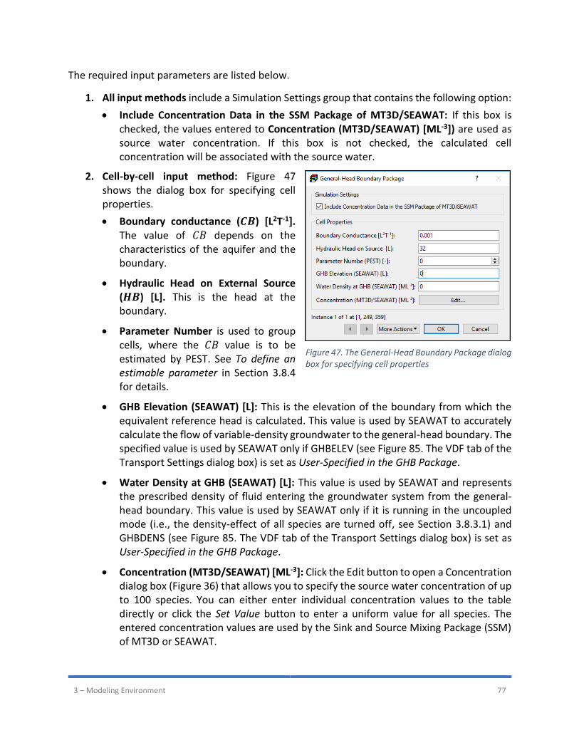
3 – Modeling Environment 77
The required input parameters are listed below.
1. All input methods include a Simulation Settings group that contains the following option:
• Include Concentration Data in the SSM Package of MT3D/SEAWAT: If this box is checked, the values entered to Concentration (MT3D/SEAWAT) [ML-3]) are used as source water concentration. If this box is not checked, the calculated cell concentration will be associated with the source water.
2. Cell-by-cell input method: Figure 47 shows the dialog box for specifying cell properties.
• Boundary conductance (𝑪𝑩) [L2T-1]. The value of 𝐶𝐵 depends on the characteristics of the aquifer and the boundary.
• Hydraulic Head on External Source (𝑯𝑩) [L]. This is the head at the boundary.
• Parameter Number is used to group cells, where the 𝐶𝐵 value is to be estimated by PEST. See To define an estimable parameter in Section 3.8.4 for details.
• GHB Elevation (SEAWAT) [L]: This is the elevation of the boundary from which the equivalent reference head is calculated. This value is used by SEAWAT to accurately calculate the flow of variable-density groundwater to the general-head boundary. The specified value is used by SEAWAT only if GHBELEV (see Figure 85. The VDF tab of the Transport Settings dialog box) is set as User-Specified in the GHB Package.
• Water Density at GHB (SEAWAT) [L]: This value is used by SEAWAT and represents the prescribed density of fluid entering the groundwater system from the general-head boundary. This value is used by SEAWAT only if it is running in the uncoupled mode (i.e., the density-effect of all species are turned off, see Section 3.8.3.1) and GHBDENS (see Figure 85. The VDF tab of the Transport Settings dialog box) is set as User-Specified in the GHB Package.
• Concentration (MT3D/SEAWAT) [ML-3]: Click the Edit button to open a Concentration dialog box (Figure 36) that allows you to specify the source water concentration of up to 100 species. You can either enter individual concentration values to the table directly or click the Set Value button to enter a uniform value for all species. The entered concentration values are used by the Sink and Source Mixing Package (SSM) of MT3D or SEAWAT.
Figure 47. The General-Head Boundary Package dialog box for specifying cell properties
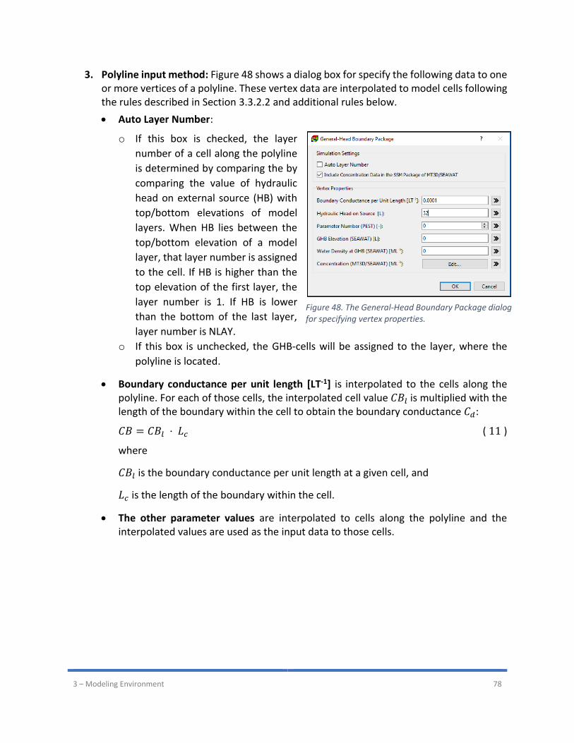
3 – Modeling Environment 78
3. Polyline input method: Figure 48 shows a dialog box for specify the following data to one or more vertices of a polyline. These vertex data are interpolated to model cells following the rules described in Section 3.3.2.2 and additional rules below.
• Auto Layer Number:
o If this box is checked, the layer
number of a cell along the polyline
is determined by comparing the by
comparing the value of hydraulic
head on external source (HB) with
top/bottom elevations of model
layers. When HB lies between the
top/bottom elevation of a model
layer, that layer number is assigned
to the cell. If HB is higher than the
top elevation of the first layer, the
layer number is 1. If HB is lower
than the bottom of the last layer,
layer number is NLAY.
o If this box is unchecked, the GHB-cells will be assigned to the layer, where the
polyline is located.
• Boundary conductance per unit length [LT-1] is interpolated to the cells along the polyline. For each of those cells, the interpolated cell value 𝐶𝐵𝑙 is multiplied with the length of the boundary within the cell to obtain the boundary conductance 𝐶𝑑:
𝐶𝐵 = 𝐶𝐵𝑙 ⋅ 𝐿𝑐 ( 11 )
where
𝐶𝐵𝑙 is the boundary conductance per unit length at a given cell, and
𝐿𝑐 is the length of the boundary within the cell.
• The other parameter values are interpolated to cells along the polyline and the interpolated values are used as the input data to those cells.
Figure 48. The General-Head Boundary Package dialog for specifying vertex properties.
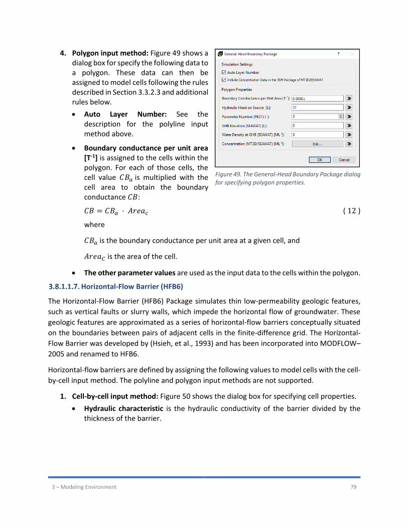
3 – Modeling Environment 79
4. Polygon input method: Figure 49 shows a dialog box for specify the following data to a polygon. These data can then be assigned to model cells following the rules described in Section 3.3.2.3 and additional rules below.
• Auto Layer Number: See the description for the polyline input method above.
• Boundary conductance per unit area [T-1] is assigned to the cells within the polygon. For each of those cells, the cell value 𝐶𝐵𝑎 is multiplied with the cell area to obtain the boundary conductance 𝐶𝐵:
𝐶𝐵 = 𝐶𝐵𝑎 ⋅ 𝐴𝑟𝑒𝑎𝑐 ( 12 )
where
𝐶𝐵𝑎 is the boundary conductance per unit area at a given cell, and
𝐴𝑟𝑒𝑎𝐶 is the area of the cell.
• The other parameter values are used as the input data to the cells within the polygon.
Horizontal-Flow Barrier (HFB6)
The Horizontal-Flow Barrier (HFB6) Package simulates thin low-permeability geologic features,
such as vertical faults or slurry walls, which impede the horizontal flow of groundwater. These
geologic features are approximated as a series of horizontal-flow barriers conceptually situated
on the boundaries between pairs of adjacent cells in the finite-difference grid. The Horizontal-
Flow Barrier was developed by (Hsieh, et al., 1993) and has been incorporated into MODFLOW–
2005 and renamed to HFB6.
Horizontal-flow barriers are defined by assigning the following values to model cells with the cell-
by-cell input method. The polyline and polygon input methods are not supported.
1. Cell-by-cell input method: Figure 50 shows the dialog box for specifying cell properties.
• Hydraulic characteristic is the hydraulic conductivity of the barrier divided by the thickness of the barrier.
Figure 49. The General-Head Boundary Package dialog for specifying polygon properties.

3 – Modeling Environment 80
• Parameter Number is used to group cells, where the hydraulic characteristic value is to be estimated by PEST. See To define an estimable parameter in Section 3.8.4 for details.
• Barrier Direction [-]: The barrier direction indicates the cell face where the barrier is located. To erase an existing barrier, select No Barrier [0].
2. Polyline and Polygon input methods are not supported.
Interbed Storage (IBS)
The Interbed Storage (IBS) Package (Leake, et al., 1991) may only be used in a transient flow
simulation. For steady state flow simulations, this menu item is deactivated.
Removal of ground water by pumping from aquifers may result in compaction of compressible
fine-grained beds that are within or adjacent to the aquifers. Compaction of the sediments and
resulting land subsidence may be permanent if the head declines result in vertical stresses
beyond the previous maximum stress. IBS is designed to simulate storage changes from both
elastic and inelastic compaction. In IBS, elastic compaction or expansion is assumed to be
proportional to change in head. The constant of proportionality is the product of the skeletal
component of elastic specific storage and the thickness of the sediments. Similarly, inelastic
compaction is assumed to be proportional to decline in head. The constant of proportionality is
the product of the skeletal component of inelastic specific storage and the thickness of the
sediments. Within a model time step, IBS appropriately apportions storage changes between
elastic and inelastic components based on the relation of simulated head to the previous
minimum (preconsolidation or critical) head.
The required input parameters for all input methods are identical and listed below.
1. All input methods: Figure 51 shows the dialog box for specifying cell, vertex, or polygon properties.
• Data Tab
o Preconsolidation Head (HC) or Critical Head [L]: Preconsolidation head is the
previous minimum head value in the aquifer. For any model cells in which the
specified preconsolidation head is greater than the initial hydraulic head, the value
of the preconsolidation head will be set to that of the initial hydraulic head; When
Figure 50. The Horizontal Flow Barrier Package dialog box
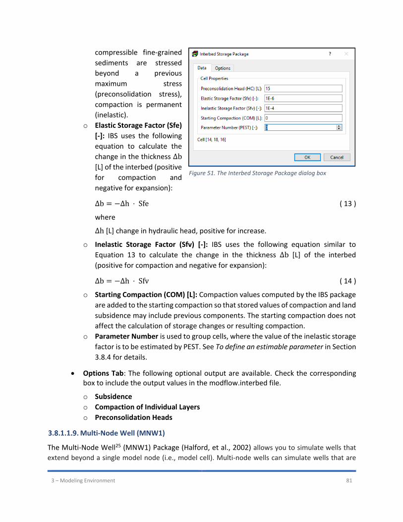
3 – Modeling Environment 81
compressible fine-grained
sediments are stressed
beyond a previous
maximum stress
(preconsolidation stress),
compaction is permanent
(inelastic).
o Elastic Storage Factor (Sfe)
[-]: IBS uses the following
equation to calculate the
change in the thickness Δb
[L] of the interbed (positive
for compaction and
negative for expansion):
Δb = −Δh ⋅ Sfe ( 13 )
where
Δh [L] change in hydraulic head, positive for increase.
o Inelastic Storage Factor (Sfv) [-]: IBS uses the following equation similar to
Equation 13 to calculate the change in the thickness Δb [L] of the interbed
(positive for compaction and negative for expansion):
Δb = −Δh ⋅ Sfv ( 14 )
o Starting Compaction (COM) [L]: Compaction values computed by the IBS package
are added to the starting compaction so that stored values of compaction and land
subsidence may include previous components. The starting compaction does not
affect the calculation of storage changes or resulting compaction.
o Parameter Number is used to group cells, where the value of the inelastic storage
factor is to be estimated by PEST. See To define an estimable parameter in Section
3.8.4 for details.
• Options Tab: The following optional output are available. Check the corresponding box to include the output values in the modflow.interbed file.
o Subsidence
o Compaction of Individual Layers
o Preconsolidation Heads
Multi-Node Well (MNW1)
The Multi-Node Well25 (MNW1) Package (Halford, et al., 2002) allows you to simulate wells that
extend beyond a single model node (i.e., model cell). Multi-node wells can simulate wells that are
Figure 51. The Interbed Storage Package dialog box
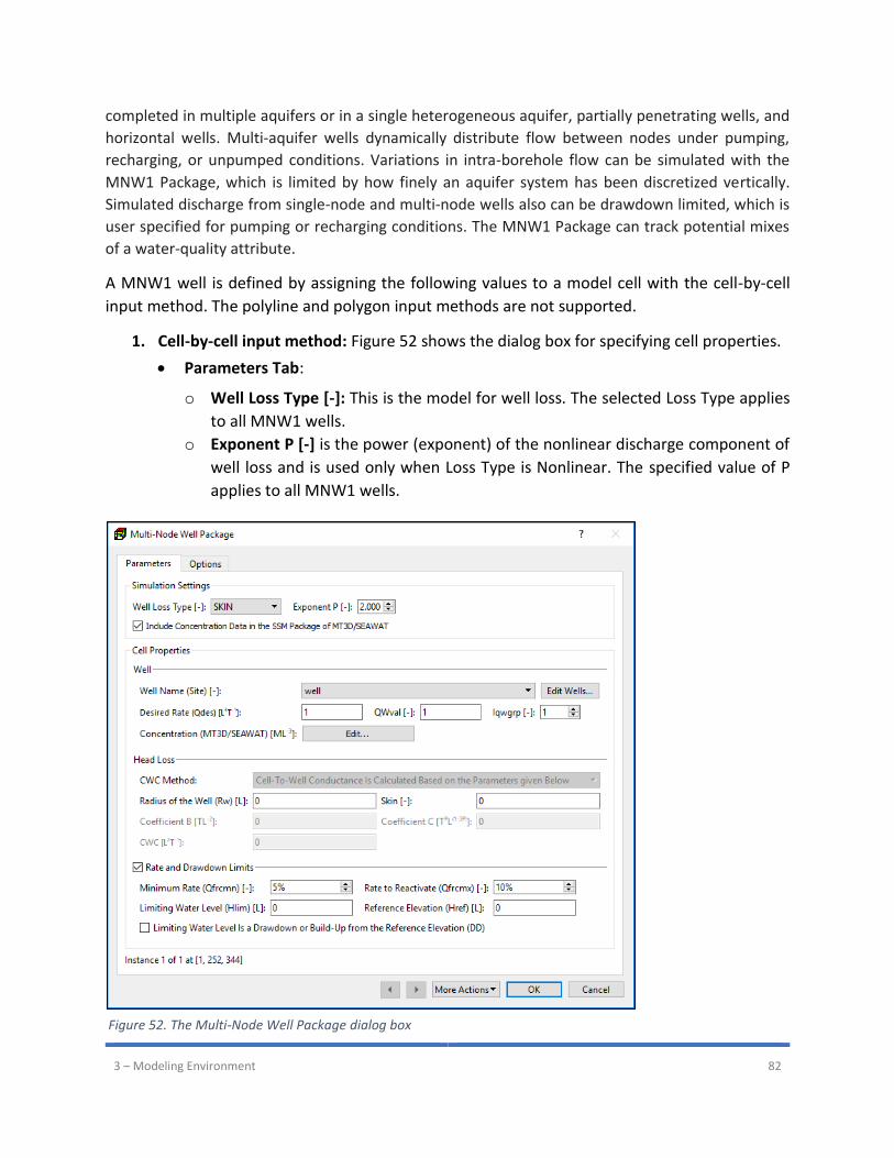
3 – Modeling Environment 82
completed in multiple aquifers or in a single heterogeneous aquifer, partially penetrating wells, and
horizontal wells. Multi-aquifer wells dynamically distribute flow between nodes under pumping,
recharging, or unpumped conditions. Variations in intra-borehole flow can be simulated with the
MNW1 Package, which is limited by how finely an aquifer system has been discretized vertically.
Simulated discharge from single-node and multi-node wells also can be drawdown limited, which is
user specified for pumping or recharging conditions. The MNW1 Package can track potential mixes
of a water-quality attribute.
A MNW1 well is defined by assigning the following values to a model cell with the cell-by-cell
input method. The polyline and polygon input methods are not supported.
1. Cell-by-cell input method: Figure 52 shows the dialog box for specifying cell properties.
• Parameters Tab:
o Well Loss Type [-]: This is the model for well loss. The selected Loss Type applies
to all MNW1 wells.
o Exponent P [-] is the power (exponent) of the nonlinear discharge component of
well loss and is used only when Loss Type is Nonlinear. The specified value of P
applies to all MNW1 wells.
Figure 52. The Multi-Node Well Package dialog box

3 – Modeling Environment 83
o Well
Edit Wells: Click this button to edit wells.
Well Name (Site) [-]: Select an existing well to which the following values apply.
Desired Rate (Qdes) [L3T-1]: The desired injection or extraction rate of the well.
Enter a positive value for injection; a negative value for extraction.
QWval [-]: Water-quality value that is to be flow-rate averaged amongst wells
in the same Iqwgrp.
Iqwgrp [-]: Water quality group identifier. Flow-rate averaged water-quality
values are reported for wells within the same Iqwgrp.
Concentration (MT3D/SEAWAT) [ML-3]: Click the Edit button to open a
Concentration dialog box (Figure 36) that allows you to specify the injected
water concentration of up to 100 species. You can either enter individual
concentration values to the table directly or click the Set Value button to enter
a uniform value for all species. The entered concentration values are used by
the Sink and Source Mixing Package (SSM) of MT3D or SEAWAT.
o Head Loss
CWC Method: Specify how the value of Cell-to-Well Conductance (CWC) is
determined. For multi-node wells, CWC Method must be "Cell-to-well
conductance is calculated based on the parameters given below".
Radius of the Well (Rw) [L]: Rw is used to calculate the cell-to-well conductance
as formulated by (Peaceman, 1983).
Skin [-] defines the friction losses to the well owing to the screen and to
formation damage. This value is used only if the Loss Type is Skin.
Coefficient B [TL-2]: This is the coefficient B of the general well-loss equation
and is used only when the Loss Type is Linear or Nonlinear. The coefficient B
accounts for head losses that occur adjacent to and within the borehole and
well.
Coefficient C [TPL(1-3P)]: This is the coefficient C accounting for the nonlinear
well-loss due to turbulent flow near the well. P is the power (exponent) of the
nonlinear discharge component of well loss. The coefficient C is used only when
the Loss Type is Nonlinear.
CWC [L2T-1]: This value is the specified cell-to-well conductance.
o Rate and Drawdown Limits
Minimum Rate (Qfrcmn) [-]: The minimum rate (as a percentage of Qdes) that
a well must exceed to remain active.
Rate to Reactivate (Qfrcmx) [-]: The minimum potential rate (as a percentage
of Qdes) that must be exceeded to reactivate a well.
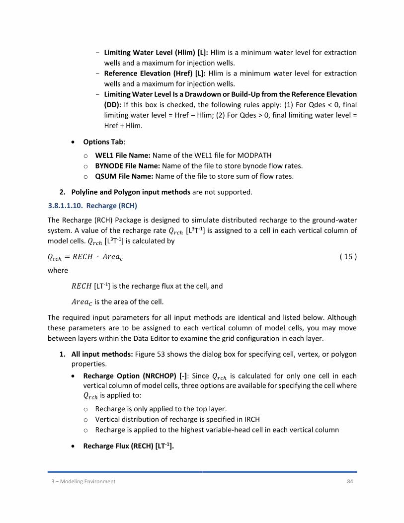
3 – Modeling Environment 84
Limiting Water Level (Hlim) [L]: Hlim is a minimum water level for extraction
wells and a maximum for injection wells.
Reference Elevation (Href) [L]: Hlim is a minimum water level for extraction
wells and a maximum for injection wells.
Limiting Water Level Is a Drawdown or Build-Up from the Reference Elevation
(DD): If this box is checked, the following rules apply: (1) For Qdes < 0, final
limiting water level = Href – Hlim; (2) For Qdes > 0, final limiting water level =
Href + Hlim.
• Options Tab:
o WEL1 File Name: Name of the WEL1 file for MODPATH
o BYNODE File Name: Name of the file to store bynode flow rates.
o QSUM File Name: Name of the file to store sum of flow rates.
2. Polyline and Polygon input methods are not supported.
Recharge (RCH)
The Recharge (RCH) Package is designed to simulate distributed recharge to the ground-water
system. A value of the recharge rate 𝑄𝑟𝑐ℎ [L3T-1] is assigned to a cell in each vertical column of
model cells. 𝑄𝑟𝑐ℎ [L3T-1] is calculated by
𝑄r𝑐ℎ = 𝑅𝐸𝐶𝐻 ⋅ 𝐴𝑟𝑒𝑎𝑐 ( 15 )
where
𝑅𝐸𝐶𝐻 [LT-1] is the recharge flux at the cell, and
𝐴𝑟𝑒𝑎𝐶 is the area of the cell.
The required input parameters for all input methods are identical and listed below. Although
these parameters are to be assigned to each vertical column of model cells, you may move
between layers within the Data Editor to examine the grid configuration in each layer.
1. All input methods: Figure 53 shows the dialog box for specifying cell, vertex, or polygon properties.
• Recharge Option (NRCHOP) [-]: Since 𝑄𝑟𝑐ℎ is calculated for only one cell in each vertical column of model cells, three options are available for specifying the cell where 𝑄𝑟𝑐ℎ is applied to:
o Recharge is only applied to the top layer.
o Vertical distribution of recharge is specified in IRCH
o Recharge is applied to the highest variable-head cell in each vertical column
• Recharge Flux (RECH) [LT-1].
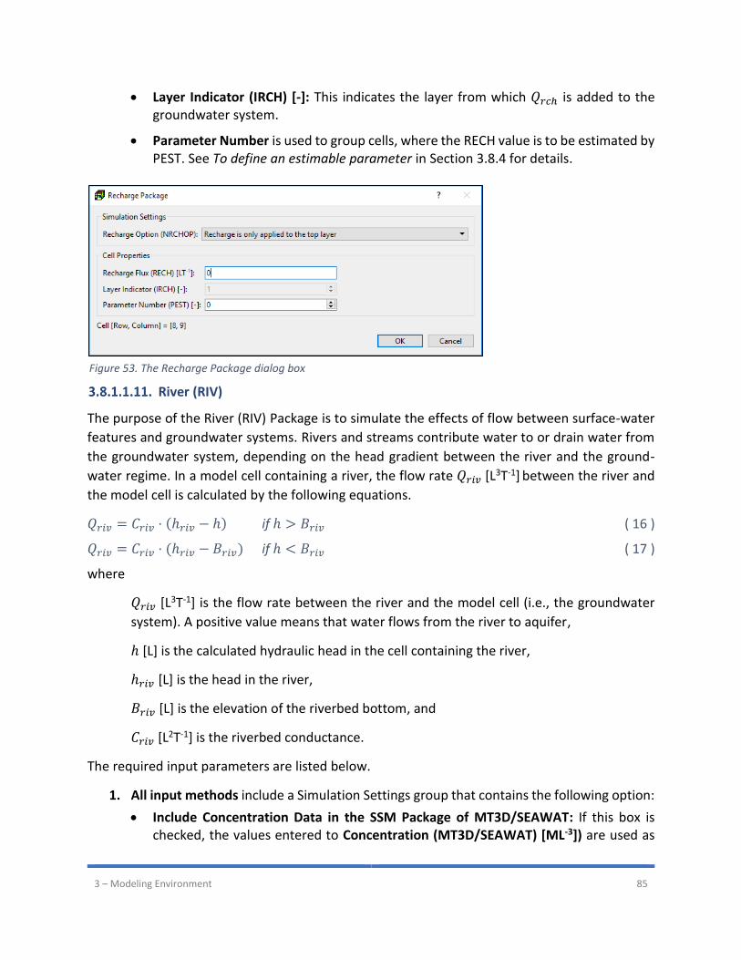
3 – Modeling Environment 85
• Layer Indicator (IRCH) [-]: This indicates the layer from which 𝑄𝑟𝑐ℎ is added to the groundwater system.
• Parameter Number is used to group cells, where the RECH value is to be estimated by PEST. See To define an estimable parameter in Section 3.8.4 for details.
River (RIV)
The purpose of the River (RIV) Package is to simulate the effects of flow between surface-water
features and groundwater systems. Rivers and streams contribute water to or drain water from
the groundwater system, depending on the head gradient between the river and the ground-
water regime. In a model cell containing a river, the flow rate 𝑄𝑟𝑖𝑣 [L3T-1] between the river and
the model cell is calculated by the following equations.
𝑄𝑟𝑖𝑣 = 𝐶𝑟𝑖𝑣 ⋅ (ℎ𝑟𝑖𝑣 − ℎ) if ℎ > 𝐵𝑟𝑖𝑣 ( 16 )
𝑄𝑟𝑖𝑣 = 𝐶𝑟𝑖𝑣 ⋅ (ℎ𝑟𝑖𝑣 − 𝐵𝑟𝑖𝑣) if ℎ < 𝐵𝑟𝑖𝑣 ( 17 )
where
𝑄𝑟𝑖𝑣 [L3T-1] is the flow rate between the river and the model cell (i.e., the groundwater
system). A positive value means that water flows from the river to aquifer,
ℎ [L] is the calculated hydraulic head in the cell containing the river,
ℎ𝑟𝑖𝑣 [L] is the head in the river,
𝐵𝑟𝑖𝑣 [L] is the elevation of the riverbed bottom, and
𝐶𝑟𝑖𝑣 [L2T-1] is the riverbed conductance.
The required input parameters are listed below.
1. All input methods include a Simulation Settings group that contains the following option:
• Include Concentration Data in the SSM Package of MT3D/SEAWAT: If this box is checked, the values entered to Concentration (MT3D/SEAWAT) [ML-3]) are used as
Figure 53. The Recharge Package dialog box

3 – Modeling Environment 86
source water concentration. If this box is not checked, the calculated cell concentration will be associated with the source water.
2. Cell-by-cell input method: Figure 54 shows the dialog box for specifying cell properties.
• Riverbed conductance 𝑪𝒓𝒊𝒗 [L2T-1] relates flow rate to the head differences between the river and the aquifer. The value of 𝐶𝑟𝑖𝑣 depends on the material and characteristics of the riverbed and the immediate environment.
• River Stage 𝒉𝒓𝒊𝒗 [L] is the hydraulic head in the river at the current cell.
• Elevation of the Riverbed Bottom (𝑩𝒓𝒊𝒗) [L] is the elevation of the bottom of the riverbed at the current cell.
• Parameter Number is used to group cells, where the Criv value is to be estimated by PEST. See To define an estimable parameter in Section 3.8.4 for details.
• Thickness of Riverbed Sediments (SEAWAT) [L]: This value is used by SEAWAT to appropriately include the effects of variable-density river leakage. The specified value is used by SEAWAT only if RBDTHK is set as User-Specified in the RIV Package. For details, see Figure 85. The VDF tab of the Transport Settings dialog box.
• River Water Density (SEAWAT) [ML-3] is the density of the river water in the current cell. This is used by SEAWAT only if it is running in the uncoupled mode (i.e., the density-effect of all species are turned off, see Section 3.8.3.1) and RIVDEN (see Figure 85. The VDF tab of the Transport Settings dialog box) is set as User-Specified in the RIV Package.
• Concentration (MT3D/SEAWAT) [ML-3]: Click the Edit button to open a Concentration dialog box (Figure 36) that allows you to specify the source water concentration of up to 100 species. You can either enter individual concentration values to the table directly or click the Set Value button to enter a uniform value for all species. The entered concentration values are used by the Sink and Source Mixing Package (SSM) of MT3D or SEAWAT.
Figure 54. The River Package dialog box for specifying cell properties
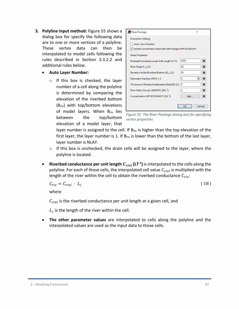
3 – Modeling Environment 87
3. Polyline input method: Figure 55 shows a dialog box for specify the following data are to one or more vertices of a polyline. These vertex data can then be interpolated to model cells following the rules described in Section 3.3.2.2 and additional rules below.
• Auto Layer Number:
o If this box is checked, the layer
number of a cell along the polyline
is determined by comparing the
elevation of the riverbed bottom
(Briv) with top/bottom elevations
of model layers. When Briv lies
between the top/bottom
elevation of a model layer, that
layer number is assigned to the cell. If Briv is higher than the top elevation of the
first layer, the layer number is 1. If Briv is lower than the bottom of the last layer,
layer number is NLAY.
o If this box is unchecked, the drain cells will be assigned to the layer, where the
polyline is located.
• Riverbed conductance per unit length 𝑪𝒓𝒊𝒗𝒍 [LT-1] is interpolated to the cells along the polyline. For each of those cells, the interpolated cell value 𝐶𝑟𝑖𝑣𝑙 is multiplied with the length of the river within the cell to obtain the riverbed conductance 𝐶𝑟𝑖𝑣:
𝐶𝑟𝑖v = 𝐶𝑟𝑖𝑣𝑙 ⋅ 𝐿𝑐 ( 18 )
where
𝐶𝑟𝑖𝑣𝑙 is the riverbed conductance per unit length at a given cell, and
𝐿𝑐 is the length of the river within the cell.
• The other parameter values are interpolated to cells along the polyline and the interpolated values are used as the input data to those cells.
Figure 55. The River Package dialog box for specifying vertex properties
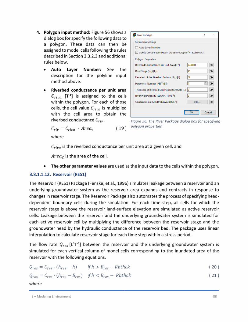
3 – Modeling Environment 88
4. Polygon input method: Figure 56 shows a dialog box for specify the following data to a polygon. These data can then be assigned to model cells following the rules described in Section 3.3.2.3 and additional rules below.
• Auto Layer Number: See the description for the polyline input method above.
• Riverbed conductance per unit area 𝑪𝒓𝒊𝒗𝒂 [T-1] is assigned to the cells within the polygon. For each of those cells, the cell value 𝐶𝑟𝑖𝑣𝑎 is multiplied with the cell area to obtain the riverbed conductance 𝐶𝑟𝑖𝑣:
𝐶𝑟𝑖𝑣 = 𝐶𝑟𝑖𝑣𝑎 ⋅ 𝐴𝑟𝑒𝑎𝑐 ( 19 )
where
𝐶𝑟𝑖𝑣𝑎 is the riverbed conductance per unit area at a given cell, and
𝐴𝑟𝑒𝑎𝐶 is the area of the cell.
• The other parameter values are used as the input data to the cells within the polygon.
Reservoir (RES1)
The Reservoir (RES1) Package (Fenske, et al., 1996) simulates leakage between a reservoir and an
underlying groundwater system as the reservoir area expands and contracts in response to
changes in reservoir stage. The Reservoir Package also automates the process of specifying head-
dependent boundary cells during the simulation. For each time step, all cells for which the
reservoir stage is above the reservoir land-surface elevation are simulated as active reservoir
cells. Leakage between the reservoir and the underlying groundwater system is simulated for
each active reservoir cell by multiplying the difference between the reservoir stage and the
groundwater head by the hydraulic conductance of the reservoir bed. The package uses linear
interpolation to calculate reservoir stage for each time step within a stress period.
The flow rate 𝑄𝑟𝑒𝑠 [L3T-1] between the reservoir and the underlying groundwater system is
simulated for each vertical column of model cells corresponding to the inundated area of the
reservoir with the following equations.
𝑄𝑟𝑒𝑠 = 𝐶𝑟𝑒𝑠 ⋅ (ℎ𝑟𝑒𝑠 − ℎ) if ℎ > 𝐵𝑟𝑒𝑠 − 𝑅𝑏𝑡ℎ𝑐𝑘 ( 20 )
𝑄𝑟𝑒𝑠 = 𝐶𝑟𝑒𝑠 ⋅ (ℎ𝑟𝑒𝑠 − 𝐵𝑟𝑒𝑠) if ℎ < 𝐵𝑟𝑒𝑠 − 𝑅𝑏𝑡ℎ𝑐𝑘 ( 21 )
where
Figure 56. The River Package dialog box for specifying polygon properties
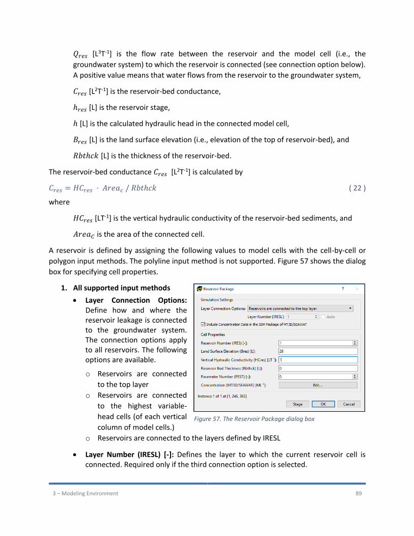
3 – Modeling Environment 89
𝑄𝑟𝑒𝑠 [L3T-1] is the flow rate between the reservoir and the model cell (i.e., the
groundwater system) to which the reservoir is connected (see connection option below).
A positive value means that water flows from the reservoir to the groundwater system,
𝐶𝑟𝑒𝑠 [L2T-1] is the reservoir-bed conductance,
ℎ𝑟𝑒𝑠 [L] is the reservoir stage,
ℎ [L] is the calculated hydraulic head in the connected model cell,
𝐵𝑟𝑒𝑠 [L] is the land surface elevation (i.e., elevation of the top of reservoir-bed), and
𝑅𝑏𝑡ℎ𝑐𝑘 [L] is the thickness of the reservoir-bed.
The reservoir-bed conductance 𝐶𝑟𝑒𝑠 [L2T-1] is calculated by
𝐶𝑟𝑒𝑠 = 𝐻𝐶𝑟𝑒𝑠 ⋅ 𝐴𝑟𝑒𝑎𝑐 / 𝑅𝑏𝑡ℎ𝑐𝑘 ( 22 )
where
𝐻𝐶𝑟𝑒𝑠 [LT-1] is the vertical hydraulic conductivity of the reservoir-bed sediments, and
𝐴𝑟𝑒𝑎𝐶 is the area of the connected cell.
A reservoir is defined by assigning the following values to model cells with the cell-by-cell or
polygon input methods. The polyline input method is not supported. Figure 57 shows the dialog
box for specifying cell properties.
1. All supported input methods
• Layer Connection Options: Define how and where the reservoir leakage is connected to the groundwater system. The connection options apply to all reservoirs. The following options are available.
o Reservoirs are connected
to the top layer
o Reservoirs are connected
to the highest variable-
head cells (of each vertical
column of model cells.)
o Reservoirs are connected to the layers defined by IRESL
• Layer Number (IRESL) [-]: Defines the layer to which the current reservoir cell is connected. Required only if the third connection option is selected.
Figure 57. The Reservoir Package dialog box
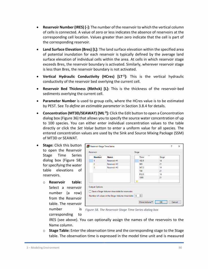
3 – Modeling Environment 90
• Reservoir Number (IRES) [-]: The number of the reservoir to which the vertical column of cells is connected. A value of zero or less indicates the absence of reservoirs at the corresponding cell location. Values greater than zero indicate that the cell is part of the corresponding reservoir.
• Land Surface Elevation (Bres) [L]: The land surface elevation within the specified area of potential inundation for each reservoir is typically defined by the average land surface elevation of individual cells within the area. At cells in which reservoir stage exceeds Bres, the reservoir boundary is activated. Similarly, wherever reservoir stage is less than Bres, the reservoir boundary is not activated.
• Vertical Hydraulic Conductivity (HCres) [LT-1]: This is the vertical hydraulic conductivity of the reservoir bed overlying the current cell.
• Reservoir Bed Thickness (Rbthck) [L]: This is the thickness of the reservoir-bed sediments overlying the current cell.
• Parameter Number is used to group cells, where the HCres value is to be estimated by PEST. See To define an estimable parameter in Section 3.8.4 for details.
• Concentration (MT3D/SEAWAT) [ML-3]: Click the Edit button to open a Concentration dialog box (Figure 36) that allows you to specify the source water concentration of up to 100 species. You can either enter individual concentration values to the table directly or click the Set Value button to enter a uniform value for all species. The entered concentration values are used by the Sink and Source Mixing Package (SSM) of MT3D or SEAWAT.
• Stage: Click this button to open the Reservoir Stage Time Series dialog box (Figure 58) for specifying the water table elevations of reservoirs.
o Reservoir table:
Select a reservoir
number (a row)
from the Reservoir
table. The reservoir
number is
corresponding to
IRES (see above). You can optionally assign the names of the reservoirs to the
Name column.
o Stage Table: Enter the observation time and the corresponding stage to the Stage
table. The observation time is expressed in the model time unit and is measured
Figure 58. The Reservoir Stage Time Series dialog box

3 – Modeling Environment 91
from the start of the model simulation. The Reservoir package requires the input
of the starting and ending stages for each stress period. The stage values for each
stress period are obtained by linear interpolation using the values specified in the
Stage table. If the starting time of a stress period is earlier than the earliest
observation time in the table, the earliest observed stage is used as the starting
stage for that stress period. Similarly, if the end time of a stress period is beyond
the latest observation time, the latest observed stage is used.
o Output Option
Save a Stage-Volume-Area table for reservoirs: If this option is checked,
reservoir stage, area, and volume (at the end of each time step) will be printed
to the Run Listing File of MODFLOW.
Number of values in the stage-volume-area table: This is the number of values
used to print the Stage-Volume-Area table. First and last stage value are
minimum and maximum elevations within area of potential inundation. A value
of 15 or greater is recommended for detailed representation of stage-volume
and stage-area relations.
Stream (STR)
The Stream (STR) Package (Prudic, 1989) is designed to account for flow in streams and to
simulate the interaction between streams and groundwater. This package was originally called
the Stream-flow Routing package, and is renamed to the Stream Package in MODFLOW-2005.
The STR Package is not a true surface water flow model, but rather is an accounting program that
tracks the flow in one or more streams which interact with groundwater. The STR Package limits
the amount of groundwater recharge to the available streamflow. It permits two or more streams
to merge into one with flow in the merged stream equal to the sum of the tributary flows. The
STR Package also permits diversions from streams. The groundwater flow model with the STR
Package has an advantage over the analytical solution in simulating the interaction between
aquifer and stream because it can be used to simulate complex systems that cannot be readily
solved analytically. The STR Package does not include a time function for streamflow but rather
streamflow entering the modeled area is assumed to be instantly available to downstream
reaches during each stress period. This assumption is generally reasonable because of the
relatively slow rate of groundwater flow. Another assumption is that leakage between streams
and aquifers is instantaneous. This assumption may not be reasonable if the streams and aquifers
are separated by a thick unsaturated zone.
The STR Package divides streams into segments and reaches. Each reach corresponds to a model
cell. A segment consists of a group of reaches connected in downstream order. Streamflow is
accounted for by specifying flow for the first reach in each segment, and then computing stream-
flow to adjacent downstream reaches in each segment as inflow in the upstream reach plus or
minus leakage from or to the aquifer in the upstream reach. Streamflow into a segment that is
3 – Modeling Environment 92
formed from tributary streams is computed by adding the outflows from the last reach in each
of the specified tributary segments. If a segment is a diversion, then the specified flow into the
first reach of the segment is subtracted from flow in the main stream. However, if the specified
flow of the diversion is greater than the flow out of the segment from which flow is to be diverted
then no flow is diverted from that segment.
For a model cell containing a reach, the flow rate 𝑄𝑠𝑡𝑟 [L3T-1] between the reach and the model
cell is calculated by the following equations.
𝑄𝑠𝑡𝑟 = 𝐶𝑠𝑡𝑟 ⋅ (ℎ𝑠𝑡𝑟 − ℎ) if ℎ > 𝐵𝑠𝑡𝑟 ( 23 )
𝑄𝑠𝑡𝑟 = 𝐶𝑠𝑡𝑟 ⋅ (ℎ𝑠𝑡𝑟 − 𝐵𝑠𝑡𝑟) if ℎ ≤ 𝐵𝑠𝑡𝑟 ( 24 )
where
𝑄𝑠𝑡𝑟 [L3T-1] is the flow rate between the reach and the model cell (i.e., the groundwater
system). A positive value means that water flows from the reach to aquifer,
𝐶𝑠𝑡𝑟 [L2T-1] is the stream conductance.
ℎ [L] is the calculated hydraulic head in the cell containing the reach,
ℎ𝑠𝑡𝑟 [L] is the stream stage (i.e., hydraulic head in the reach), and
𝐵𝑠𝑡𝑟 [L] is the elevation of the bottom of streambed sediments.
The cell-by-cell or polyline input methods may be used to specify the following stream data. The
polygon input method is not supported. The polyline input method is recommended as it can
assign the reach numbers in the required sequential order automatically.
1. Cell-by-cell input methods: Figure 59 shows the dialog box for specifying cell properties.
• Calculate Stream Stage in Reaches: If checked, the stream stage in each reach is calculated based on Manning’s formula under the assumption of a rectangular stream channel. This option applies to the entire STR package.
• Segment (Cell Properties)
o Segment Number [-]: The number of the segment to which the current cell
belongs. Enter 0 to remove the cell from the segment.
o Inflow to this Segment [L3T-1]: The streamflow entering the segment. Enter -1, if
inflow into this segment is the sum of outflow from its tributary segments. If a
segment is a diversion and the Simulate diversions from segments box (see below)
is checked, then the specified inflow is subtracted from flow in the main stream.
However, if the specified inflow of the diversion is greater than the flow out of the
segment from which flow is to be diverted, then no flow is diverted from that
segment.
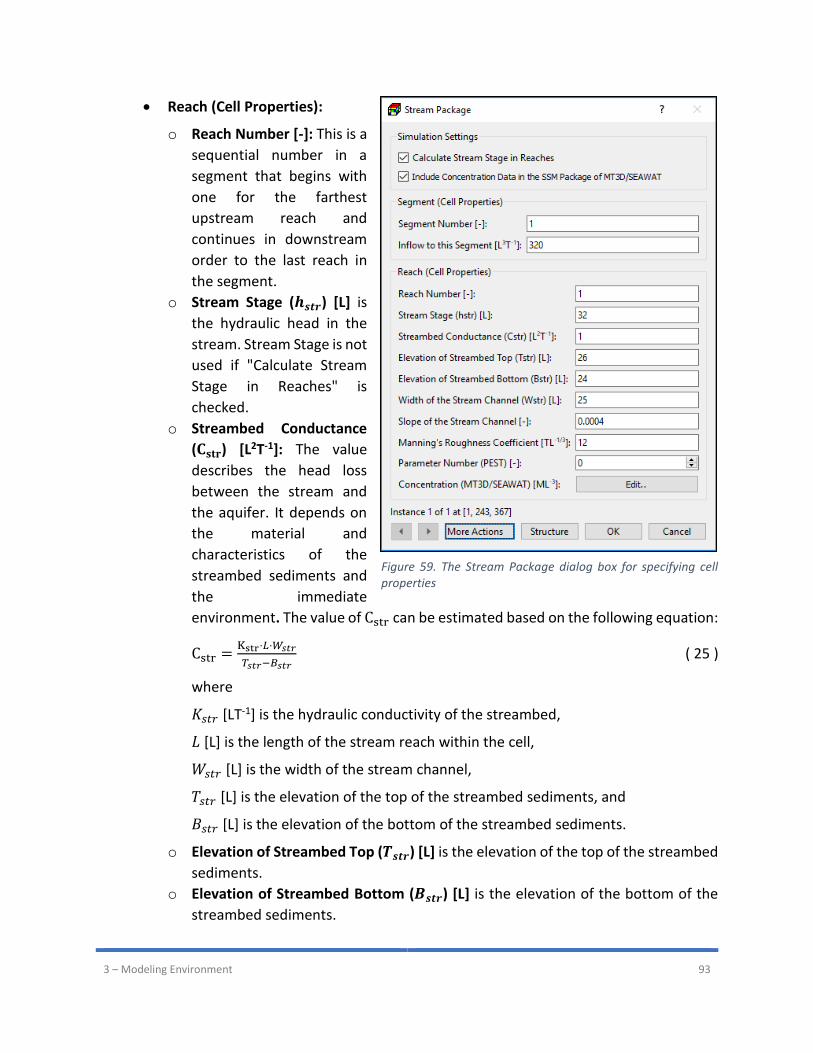
3 – Modeling Environment 93
• Reach (Cell Properties):
o Reach Number [-]: This is a
sequential number in a
segment that begins with
one for the farthest
upstream reach and
continues in downstream
order to the last reach in
the segment.
o Stream Stage (𝒉𝒔𝒕𝒓) [L] is
the hydraulic head in the
stream. Stream Stage is not
used if "Calculate Stream
Stage in Reaches" is
checked.
o Streambed Conductance
(𝐂𝐬𝐭𝐫) [L2T-1]: The value
describes the head loss
between the stream and
the aquifer. It depends on
the material and
characteristics of the
streambed sediments and
the immediate
environment. The value of Cstr can be estimated based on the following equation:
Cstr =Kstr⋅𝐿⋅𝑊𝑠𝑡𝑟
𝑇𝑠𝑡𝑟−𝐵𝑠𝑡𝑟 ( 25 )
where
𝐾𝑠𝑡𝑟 [LT-1] is the hydraulic conductivity of the streambed,
𝐿 [L] is the length of the stream reach within the cell,
𝑊𝑠𝑡𝑟 [L] is the width of the stream channel,
𝑇𝑠𝑡𝑟 [L] is the elevation of the top of the streambed sediments, and
𝐵𝑠𝑡𝑟 [L] is the elevation of the bottom of the streambed sediments.
o Elevation of Streambed Top (𝑻𝒔𝒕𝒓) [L] is the elevation of the top of the streambed
sediments.
o Elevation of Streambed Bottom (𝑩𝒔𝒕𝒓) [L] is the elevation of the bottom of the
streambed sediments.
Figure 59. The Stream Package dialog box for specifying cell properties
3 – Modeling Environment 94
o Width of the Stream Channel (𝑾𝒔𝒕𝒓) [L], Slope of the Stream Channel (𝑺𝒔𝒕𝒓) [-],
and Manning's Roughness Coefficient (n) [TL-1/3]: These parameters are used only
when the box Calculate Stream Stage in Reaches is checked. To obtain the stream
stage, the stream water depth (𝑑𝑠𝑡𝑟) is calculated using the Manning’s equation
under the assumption of a rectangular stream channel. The calculated water
depth is added to 𝑇𝑠𝑡𝑟 to get the stream stage. The Manning’s equation for a
rectangular stream channel is
𝑑str = [𝑄 ⋅ 𝑛
𝑊𝑠𝑡𝑟 ⋅ 𝑆𝑠𝑡𝑟1/2] ( 26 )
where
𝑄 [L3T-1] is the calculated stream discharge, and
𝑆𝑠𝑡𝑟 [-] is the slop of the stream channel.
The unit for Manning's roughness coefficient (n) is often left off, as n is usually given in SI units, for example [s/m1/3]. If other units are used in the model, you should convert the value of n accordingly and enter the converted value to the model. For example, if your model uses [day] and [ft] for the time and length units, the following conversion applies
n = 1 [𝑠
𝑚1/3] =1
86400×3.281/3 [𝑑𝑎𝑦
𝑓𝑡1/3] =1
128383[
𝑑𝑎𝑦
𝑓𝑡1/3] ( 27 )
Some conversion examples for other units are given below
n = 1 [𝑠
𝑚1/3] =
1
86400[
𝑑𝑎𝑦
𝑚1/3] =
1
1.486[
𝑠
𝑓𝑡1/3] ( 28 )
o Parameter Number (PEST) [-] is used to group cells, where the Cstr value is to be
estimated by PEST. See To define an estimable parameter in Section 3.8.4 for
details.
o Concentration (MT3D/SEAWAT) [ML-3]: Click the Edit button to open a
Concentration dialog box (Figure 36) that allows you to specify the source water
concentration of up to 100 species. You can either enter individual concentration
values to the table directly or click the Set Value button to enter a uniform value
for all species. The entered concentration values are used by the Sink and Source
Mixing Package (SSM) of MT3D or SEAWAT.
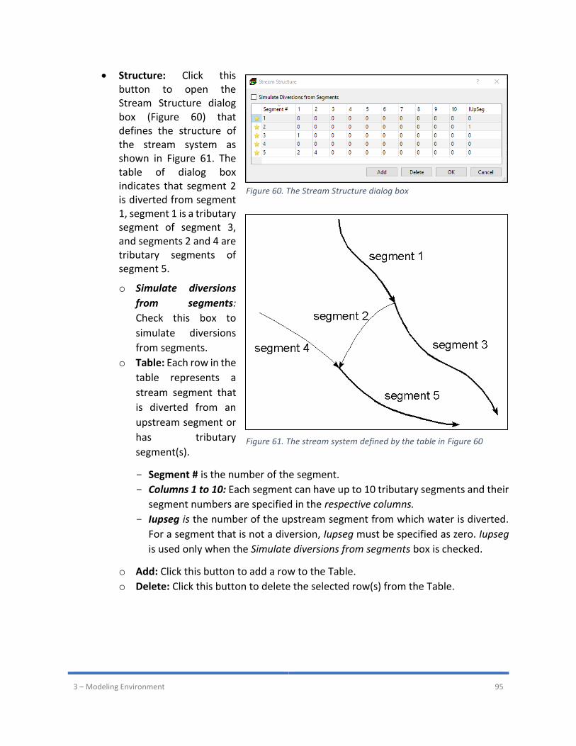
3 – Modeling Environment 95
• Structure: Click this button to open the Stream Structure dialog box (Figure 60) that defines the structure of the stream system as shown in Figure 61. The table of dialog box indicates that segment 2 is diverted from segment 1, segment 1 is a tributary segment of segment 3, and segments 2 and 4 are tributary segments of segment 5.
o Simulate diversions
from segments:
Check this box to
simulate diversions
from segments.
o Table: Each row in the
table represents a
stream segment that
is diverted from an
upstream segment or
has tributary
segment(s).
Segment # is the number of the segment.
Columns 1 to 10: Each segment can have up to 10 tributary segments and their
segment numbers are specified in the respective columns.
Iupseg is the number of the upstream segment from which water is diverted.
For a segment that is not a diversion, Iupseg must be specified as zero. Iupseg
is used only when the Simulate diversions from segments box is checked.
o Add: Click this button to add a row to the Table.
o Delete: Click this button to delete the selected row(s) from the Table.
Figure 60. The Stream Structure dialog box
Figure 61. The stream system defined by the table in Figure 60
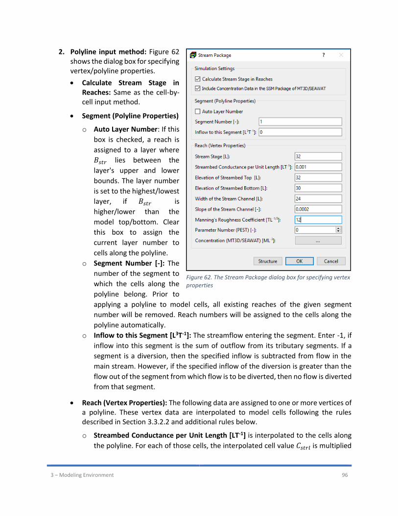
3 – Modeling Environment 96
2. Polyline input method: Figure 62 shows the dialog box for specifying vertex/polyline properties.
• Calculate Stream Stage in Reaches: Same as the cell-by-cell input method.
• Segment (Polyline Properties)
o Auto Layer Number: If this
box is checked, a reach is
assigned to a layer where
𝐵𝑠𝑡𝑟 lies between the
layer's upper and lower
bounds. The layer number
is set to the highest/lowest
layer, if 𝐵𝑠𝑡𝑟 is
higher/lower than the
model top/bottom. Clear
this box to assign the
current layer number to
cells along the polyline.
o Segment Number [-]: The
number of the segment to
which the cells along the
polyline belong. Prior to
applying a polyline to model cells, all existing reaches of the given segment
number will be removed. Reach numbers will be assigned to the cells along the
polyline automatically.
o Inflow to this Segment [L3T-1]: The streamflow entering the segment. Enter -1, if
inflow into this segment is the sum of outflow from its tributary segments. If a
segment is a diversion, then the specified inflow is subtracted from flow in the
main stream. However, if the specified inflow of the diversion is greater than the
flow out of the segment from which flow is to be diverted, then no flow is diverted
from that segment.
• Reach (Vertex Properties): The following data are assigned to one or more vertices of a polyline. These vertex data are interpolated to model cells following the rules described in Section 3.3.2.2 and additional rules below.
o Streambed Conductance per Unit Length [LT-1] is interpolated to the cells along
the polyline. For each of those cells, the interpolated cell value 𝐶𝑠𝑡𝑟𝑙 is multiplied
Figure 62. The Stream Package dialog box for specifying vertex properties
3 – Modeling Environment 97
with the length of the reach within the cell to obtain the streambed conductance
𝐶𝑠𝑡𝑟:
𝐶𝑠𝑡𝑟 = 𝐶𝑠𝑡𝑟𝑙 ⋅ 𝐿𝑐 ( 29 )
where
𝐶𝑠𝑡𝑟𝑙 is the streambed conductance per unit length at a given cell, and
𝐿𝑐 is the length of the reach within the cell.
o The other parameter values are interpolated to cells along the polyline and the
interpolated values are used as the input data to those cells.
• Concentration (MT3D/SEAWAT) [ML-3]: Same as the cell-by-cell input method.
• Structure: Same as the cell-by-cell input method.
Seawater Intrusion 2 (SWI2)
The SWI2 Package (Bakker, et al., 2013) allows three-dimensional vertically integrated variable-density groundwater flow and seawater intrusion in coastal multi-aquifer systems to be simulated using MODFLOW-2005. The main advantage of the formulation used in the SWI2 Package compared to models that solve flow and transport equations is that the SWI2 Package represents three-dimensional vertically integrated variable-density flow without the need to discretize the aquifer vertically. Vertically integrated variable-density groundwater flow is based on the Dupuit approximation in which an aquifer is vertically discretized into zones of differing densities, separated from each other by defined surfaces representing interfaces or density isosurfaces. The numerical approach used in the SWI2 Package does not account for diffusion and dispersion and should not be used where these processes are important. The resulting differential equations are equivalent in form to the groundwater flow equation for uniform-density flow. The approach implemented in the SWI2 Package allows density effects to be incorporated into MODFLOW-2005 through the addition of pseudo-source terms to the groundwater flow equation without the need to solve a separate advective-dispersive transport equation. Vertical and horizontal movement of defined density surfaces is calculated separately using a combination of fluxes calculated through solution of the groundwater flow equation and a simple tip and toe tracking algorithm. The required input parameters for all input methods are identical and listed below.
1. All input methods:
• Data Tab (Figure 63)
o Number of ZETA Surfaces (NSRF) [-]: This is the number of active surfaces (i.e.,
interfaces between zones).
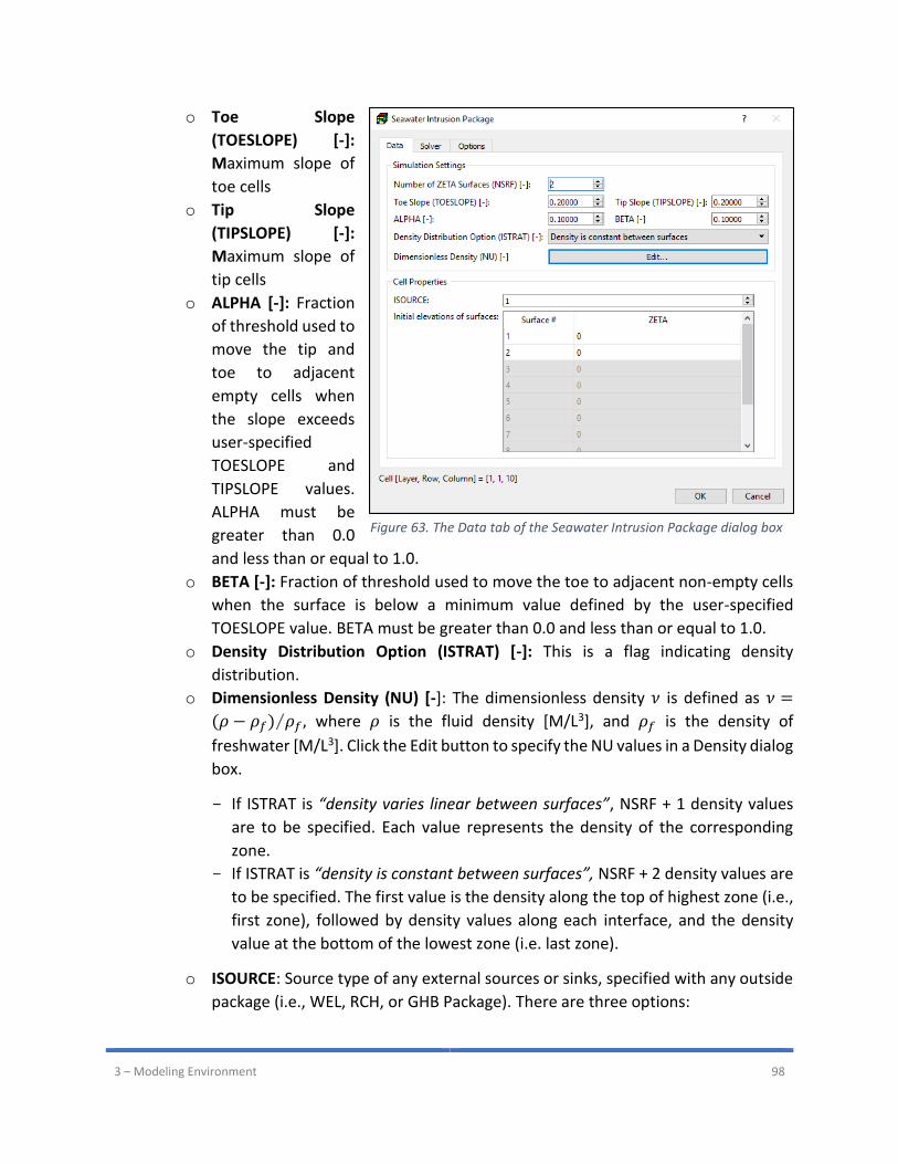
3 – Modeling Environment 98
o Toe Slope
(TOESLOPE) [-]:
Maximum slope of
toe cells
o Tip Slope
(TIPSLOPE) [-]:
Maximum slope of
tip cells
o ALPHA [-]: Fraction
of threshold used to
move the tip and
toe to adjacent
empty cells when
the slope exceeds
user-specified
TOESLOPE and
TIPSLOPE values.
ALPHA must be
greater than 0.0
and less than or equal to 1.0.
o BETA [-]: Fraction of threshold used to move the toe to adjacent non-empty cells
when the surface is below a minimum value defined by the user-specified
TOESLOPE value. BETA must be greater than 0.0 and less than or equal to 1.0.
o Density Distribution Option (ISTRAT) [-]: This is a flag indicating density
distribution.
o Dimensionless Density (NU) [-]: The dimensionless density 𝜈 is defined as 𝜈 =
(𝜌 − 𝜌𝑓) 𝜌𝑓⁄ , where 𝜌 is the fluid density [M/L3], and 𝜌𝑓 is the density of
freshwater [M/L3]. Click the Edit button to specify the NU values in a Density dialog
box.
If ISTRAT is “density varies linear between surfaces”, NSRF + 1 density values
are to be specified. Each value represents the density of the corresponding
zone.
If ISTRAT is “density is constant between surfaces”, NSRF + 2 density values are
to be specified. The first value is the density along the top of highest zone (i.e.,
first zone), followed by density values along each interface, and the density
value at the bottom of the lowest zone (i.e. last zone).
o ISOURCE: Source type of any external sources or sinks, specified with any outside
package (i.e., WEL, RCH, or GHB Package). There are three options:
Figure 63. The Data tab of the Seawater Intrusion Package dialog box
3 – Modeling Environment 99
If ISOURCE > 0: Sources and sinks have the same fluid density as the zone
ISOURCE. If such a zone is not present in the cell, sources and sinks have the
same fluid density as the active zone at the top of the aquifer.
If ISOURCE = 0: Sources and sinks have the same fluid density as the active zone
at the top of the aquifer.
If ISOURCE < 0: Sources have the same fluid density as the zone with a number
equal to the absolute value of ISOURCE. Sinks have the same fluid density as
the active zone at the top of the aquifer. This option is useful for the modeling
of the ocean bottom where infiltrating water is salt, yet exfiltrating water is of
the same type as the water at the top of the aquifer.
o Initial Elevations of Surfaces: Use the table to specify the initial elevations of the
ZETA surfaces (i.e., interface between zones).
An elevation for each surface needs to be specified for every cell in the model,
even though a zeta surface is two-dimensional in most cases.
When the specified Zeta surface value is above the top of the model layer, SWI2
requires the Zeta surface value to be set to the top of model layer in its input
file, similarly when the specified Zeta surface value is below the bottom of
model layer, SWI2 requires the Zeta surface value to be set to the bottom of
model layer. PM will automatically adjust the Zeta surface based on this
requirement when creating the input file for SWI2. Therefore, if a surface is
present at only one point in the vertical everywhere, the same grid of ZETA
values may be entered for every model layer.
It is important to start with a reasonably smooth variation of the ZETA surface
because it is not physically reasonable for a surface to be discontinuous or have
sharp changes in gradient. When an irregular ZETA surface is entered,
additional time in a transient simulation may be required before a physically
realistic ZETA elevation is achieved in each cell, and it may take small time steps
to reach an accurate solution.
• Solver Tab (Figure 64)
o Solver (NSOLVER) [-]: The solver used to solve for ZETA surfaces.
o Printout Option (MUTSOL): This controls printing of convergence information
from the solver.
o Printout Interval (IRPSOL): The extreme head change and residual (positive or
negative) are printed for each iteration of a time step whenever the time step is
an even multiple of the printout interval. The printout also occurs at the end of
each stress period regardless of the value of the printout interval.
o NPCOND: This is the matrix preconditioning method.
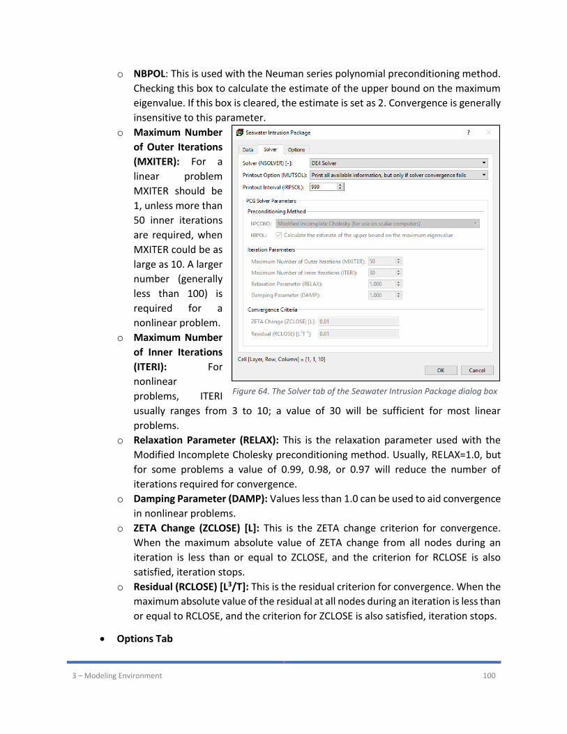
3 – Modeling Environment 100
o NBPOL: This is used with the Neuman series polynomial preconditioning method.
Checking this box to calculate the estimate of the upper bound on the maximum
eigenvalue. If this box is cleared, the estimate is set as 2. Convergence is generally
insensitive to this parameter.
o Maximum Number
of Outer Iterations
(MXITER): For a
linear problem
MXITER should be
1, unless more than
50 inner iterations
are required, when
MXITER could be as
large as 10. A larger
number (generally
less than 100) is
required for a
nonlinear problem.
o Maximum Number
of Inner Iterations
(ITERI): For
nonlinear
problems, ITERI
usually ranges from 3 to 10; a value of 30 will be sufficient for most linear
problems.
o Relaxation Parameter (RELAX): This is the relaxation parameter used with the
Modified Incomplete Cholesky preconditioning method. Usually, RELAX=1.0, but
for some problems a value of 0.99, 0.98, or 0.97 will reduce the number of
iterations required for convergence.
o Damping Parameter (DAMP): Values less than 1.0 can be used to aid convergence
in nonlinear problems.
o ZETA Change (ZCLOSE) [L]: This is the ZETA change criterion for convergence.
When the maximum absolute value of ZETA change from all nodes during an
iteration is less than or equal to ZCLOSE, and the criterion for RCLOSE is also
satisfied, iteration stops.
o Residual (RCLOSE) [L3/T]: This is the residual criterion for convergence. When the
maximum absolute value of the residual at all nodes during an iteration is less than
or equal to RCLOSE, and the criterion for ZCLOSE is also satisfied, iteration stops.
• Options Tab
Figure 64. The Solver tab of the Seawater Intrusion Package dialog box

3 – Modeling Environment 101
o Adaptive Time Stepping: Check this box to enable adaptive time stepping
algorithm that dynamically adjust the number of SWI2 time steps in a MODFLOW
time step. The algorithm has no effect on the lengths of MODFLOW time steps and
stress periods. Use of this option will increase the number of SWI2 time steps used
during a MODFLOW time step when the tip or toe movement exceeds a user-
defined value.
o NADPTMX [-]: Maximum number of SWI2 time steps per MODFLOW time step.
o NADPTMN [-]: Minimum number of SWI2 time steps per MODFLOW time step.
NADPTMN must be less than or equal to NADPTMX.
o ADPTFCT [-]: ADPTFCT is the factor used to evaluate tip and toe thicknesses and
control the number of SWI2 time steps per MODFLOW time step.
Time-Variant Specified Head (CHD)
For transient simulations, the Time-Variant Specified-Head (CHD) Package described in Appendix
C of (Leake, et al., 1991) allows constant head cells to take on different head values for each time
step. It provides a means of simulating head variations with time that can be approximated with
piecewise linear segments. The CHD Package does not alter the way constant-head boundaries
are formulated in MODFLOW.
The required input parameters for all input methods are identical and listed below.
1. All input methods27: Figure 65 shows the dialog box for specifying cell, vertex, or polygon properties.
• Flag [-]: A non-zero value indicates that a cell is specified as a time-variant specified-head boundary.
o A no-flow cell
cannot be
converted to a CHD-cell.
o If a cell is specified as a time-variant specified-head boundary for a stress period
and omitted in the specification for a subsequent period, it remains a constant-
head boundary with a head equal to the end head of the last stress period for
which it was specified.
27 If multiple instances of CHD are assigned to a single cell, only one instance with the average values of ℎ𝑠, ℎ𝑒, and d of all instances will be use in the simulation.
Figure 65. The Time-Variant Specified Head Package dialog box
3 – Modeling Environment 102
• Start Head (𝒉𝒔) [L]27 and End Head (𝒉𝒆) [L]27: These values are the prescribed hydraulic head of the cell at the start and end of a stress period, respectively. For each time step within the stress period, the prescribed hydraulic head ℎ at the cell is determined by
ℎ = ℎ𝑠 + (ℎ𝑒 − ℎ𝑠) ⋅𝑃𝐸𝑅𝑇𝐼𝑀
𝑃𝐸𝑅𝐿𝐸𝑁 ( 30 )
where
𝑃𝐸𝑅𝑇𝐼𝑀 is the starting time of the time step, and
𝑃𝐸𝑅𝐿𝐸𝑁 is the length of the stress period.
The interpolated head values remain constant during the time step.
• Head Conversion (SEAWAT): This option determines how SEAWAT converts the specified values of ℎ𝑠 and ℎ𝑒 to reference head. Four options are available:
o Use calculated water density at the cell
o Use the specified water density value
o Use the average of the calculated water density of the overlying cells
o Input head values are reference head. No conversion
• Water Density (d) [ML-3] (SEAWAT)27: Required only if the Head Conversion option is Use the specified water density value. SEAWAT uses this value to convert input head values to reference head.
Unsaturated-Zone Flow (UZF1)
The Unsaturated-Zone Flow (UZF1) Package (Niswonger, et al., 2006) was developed to simulate
water flow and storage in the unsaturated zone and to partition flow into evapotranspiration and
recharge. The package also accounts for land surface runoff to streams and lakes.
A kinematic wave approximation to Richards’ equation is solved by the method of characteristics
to simulate vertical unsaturated flow. The approach assumes that unsaturated flow occurs in
response to gravity potential gradients only and ignores negative potential gradients; the
approach further assumes uniform hydraulic properties in the unsaturated zone for each vertical
column of model cells. The Brooks-Corey function is used to define the relation between
unsaturated hydraulic conductivity and water content. Residual water content is calculated
internally by the UZF1 Package based on the difference between saturated water content and
specific yield.
The UZF1 Package is a substitution for the Recharge and Evapotranspiration Packages. The UZF1
Package differs from the Recharge Package in that an infiltration rate is applied at land surface
instead of a specified recharge rate directly to ground water. The applied infiltration rate is
further limited by the saturated vertical hydraulic conductivity. The UZF1 Package differs from
the Evapotranspiration Package in that evapotranspiration losses are first removed from the
unsaturated zone above the evapotranspiration extinction depth, and if the demand is not met,
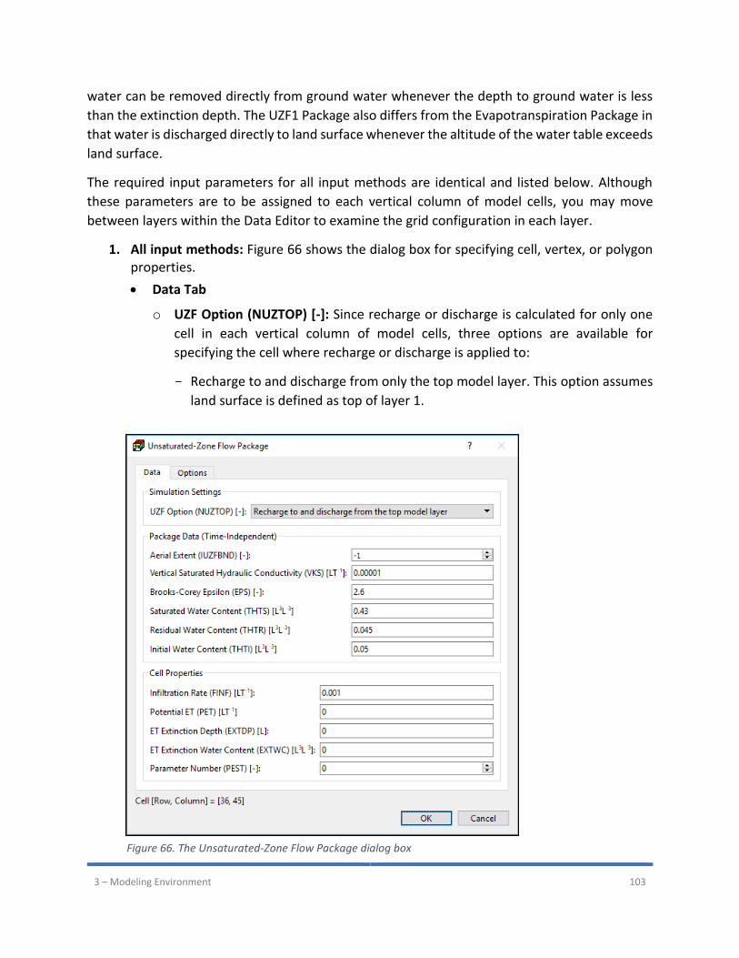
3 – Modeling Environment 103
water can be removed directly from ground water whenever the depth to ground water is less
than the extinction depth. The UZF1 Package also differs from the Evapotranspiration Package in
that water is discharged directly to land surface whenever the altitude of the water table exceeds
land surface.
The required input parameters for all input methods are identical and listed below. Although
these parameters are to be assigned to each vertical column of model cells, you may move
between layers within the Data Editor to examine the grid configuration in each layer.
1. All input methods: Figure 66 shows the dialog box for specifying cell, vertex, or polygon properties.
• Data Tab
o UZF Option (NUZTOP) [-]: Since recharge or discharge is calculated for only one
cell in each vertical column of model cells, three options are available for
specifying the cell where recharge or discharge is applied to:
Recharge to and discharge from only the top model layer. This option assumes
land surface is defined as top of layer 1.
Figure 66. The Unsaturated-Zone Flow Package dialog box
3 – Modeling Environment 104
Recharge to and discharge from the specified layer in variable IUZFBND. This
option assumes land surface is defined as top of layer specified in IUZFBND.
Recharge to and discharge from the highest active cell in each vertical column.
Land surface is determined as top of layer specified in IUZFBND. A constant
head node intercepts any recharge and prevents deeper percolation.
o Package Data (Time-Independent)
Aerial Extent (IUZFBND) [-]: This value is used to define the aerial extent of the
active model in which recharge and discharge will be simulated.
▪ If IUZFBND = 0, recharge and discharge will not be simulated.
▪ If IUZFBND < 0, the calculated infiltration will be added as recharge directly
to groundwater, and storage changes in the unsaturated zone will be
neglected.
▪ If NUZTOP = 2, the value of IUZFBND indicates the layer where recharge and
discharge occurs.
▪ If NUZTOP ≥ 2, the value of IUZFBND indicates the layer whose top is the
land surface.
Vertical Saturated Hydraulic Conductivity (VKS) [LT-1]: This is the vertical
saturated hydraulic conductivity of the UZF cell.
Brooks-Corey Epsilon (EPS) [-]: The epsilon exponent is used in the relation of
water content to hydraulic conductivity.
Saturated Water Content (THTS) [L3L-3]: The saturated water content is
approximately the same as the porosity.
Residual Water Content (THTR) [L3L-3]: the residual water content, commonly
defined as the water content θ for which the gradient dθ/dh becomes zero,
where h is the pressure head.
Initial Water Content (THTI) [L3L-3]: The water content at the beginning of the
simulation.
o Cell Properties (for Cell-by-Cell input method), Polygon Properties (for Polygon
input method), or Vertex Properties (for Polyline input method)
Infiltration Rate (FINF) [LT-1]: This is the specified infiltration rate.
Potential ET (PET) [LT-1]: Potential evapotranspiration flux.
ET Extinction Depth (EXTDP) [L]: The quantity of ET removed from a cell is
limited by the volume of water stored in the unsaturated zone above the
extinction depth. If groundwater is within the ET extinction depth, then the rate
removed is based on a linear decrease in the maximum rate at land surface and
zero at the ET extinction depth.
3 – Modeling Environment 105
ET Extinction Water Content (EXTWC) [L3L-3]: The water content below which
ET cannot be removed from the unsaturated zone.
Parameter Number is used to group cells, where the FINF value is to be
estimated by PEST. See To define an estimable parameter in Section 3.8.4 for
details.
• Options Tab
o Average Surface Depression Depth of the UZF cells (SURFDEP) [L]: This is the
average undulation depth within the cell.
o Number of Trailing Waves (NTRAIL2) [-]: This is the number of trailing waves used
to define the water-content profile following a decrease in the infiltration rate.
o Number of Wave Sets (NSETS2) [-]: This is the number of wave sets used to
simulate multiple infiltration periods.
o Deactivate surface leakage calculation (NOSURFLEAK): When the head is higher
than the land surface, water seepage to the land surface may be removed from
the groundwater system if this box is not checked.
o Route water through unsaturated zone (IUZFOPT): Check this box to route water
through unsaturated zone (i.e., IUZFOPT = 1 if checked).
o Simulate Evapotranspiration (IETFLG): Specifies whether evapotranspiration (ET)
will be simulated. ET will be simulated if this box is checked, otherwise it will not
be simulated.
Well (WEL)
The Well (WEL) Package is designed to simulate features such as wells that withdraw water from
or add water to the aquifer at a constant rate during a stress period, where the rate is
independent of both the cell area and the head in the cell. The Package can be used to simulate
any features for which the recharge or discharge can be directly specified. Consider using the
MNW1 Package (Section 3.8.1.1.9) for wells that penetrate multiple model layers.
The required input parameters are listed below.
1. All input methods include a Simulation Settings group that contains the following option:
• Include Concentration Data in the SSM Package of MT3D/SEAWAT: If this box is checked, the values entered to Concentration (MT3D/SEAWAT) [ML-3]) are used as source water concentration. If this box is not checked, the calculated cell concentration will be associated with the source water.
2. Cell-by-cell input method: Figure 67 shows the dialog box for specifying cell properties.
• Flow Rate (Q) [L3T-1]: Negative values are used to indicate pumping wells, while positive cell values indicate injection wells. The injection or pumping rate of a well is independent of both the cell area and the hydraulic head in the cell. MODFLOW assumes that a well penetrates the full thickness of the cell. To simulate wells that
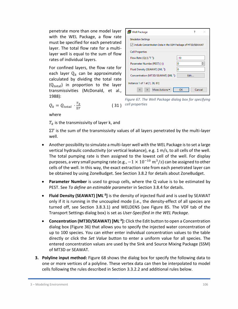
3 – Modeling Environment 106
penetrate more than one model layer with the WEL Package, a flow rate must be specified for each penetrated layer. The total flow rate for a multi-layer well is equal to the sum of flow rates of individual layers.
For confined layers, the flow rate for each layer Q𝑘 can be approximately calculated by dividing the total rate (Qtotal) in proportion to the layer transmissivities (McDonald, et al., 1988):
𝑄𝑘 = 𝑄𝑡𝑜𝑡𝑎𝑙 ⋅𝑇𝑘
Σ𝑇 ( 31 )
where
𝑇𝑘 is the transmissivity of layer k, and
Σ𝑇 is the sum of the transmissivity values of all layers penetrated by the multi-layer well.
• Another possibility to simulate a multi-layer well with the WEL Package is to set a large vertical hydraulic conductivity (or vertical leakance), e.g. 1 m/s, to all cells of the well. The total pumping rate is then assigned to the lowest cell of the well. For display purposes, a very small pumping rate (e.g., −1 × 10⁻¹⁰ 𝑚3/𝑠) can be assigned to other cells of the well. In this way, the exact extraction rate from each penetrated layer can be obtained by using ZoneBudget. See Section 3.8.2 for details about ZoneBudget.
• Parameter Number is used to group cells, where the Q value is to be estimated by PEST. See To define an estimable parameter in Section 3.8.4 for details.
• Fluid Density (SEAWAT) [ML-3] is the density of injected fluid and is used by SEAWAT only if it is running in the uncoupled mode (i.e., the density-effect of all species are turned off, see Section 3.8.3.1) and WELDENS (see Figure 85. The VDF tab of the Transport Settings dialog box) is set as User-Specified in the WEL Package.
• Concentration (MT3D/SEAWAT) [ML-3]: Click the Edit button to open a Concentration dialog box (Figure 36) that allows you to specify the injected water concentration of up to 100 species. You can either enter individual concentration values to the table directly or click the Set Value button to enter a uniform value for all species. The entered concentration values are used by the Sink and Source Mixing Package (SSM) of MT3D or SEAWAT.
3. Polyline input method: Figure 68 shows the dialog box for specify the following data to one or more vertices of a polyline. These vertex data can then be interpolated to model cells following the rules described in Section 3.3.2.2 and additional rules below.
Figure 67. The Well Package dialog box for specifying cell properties
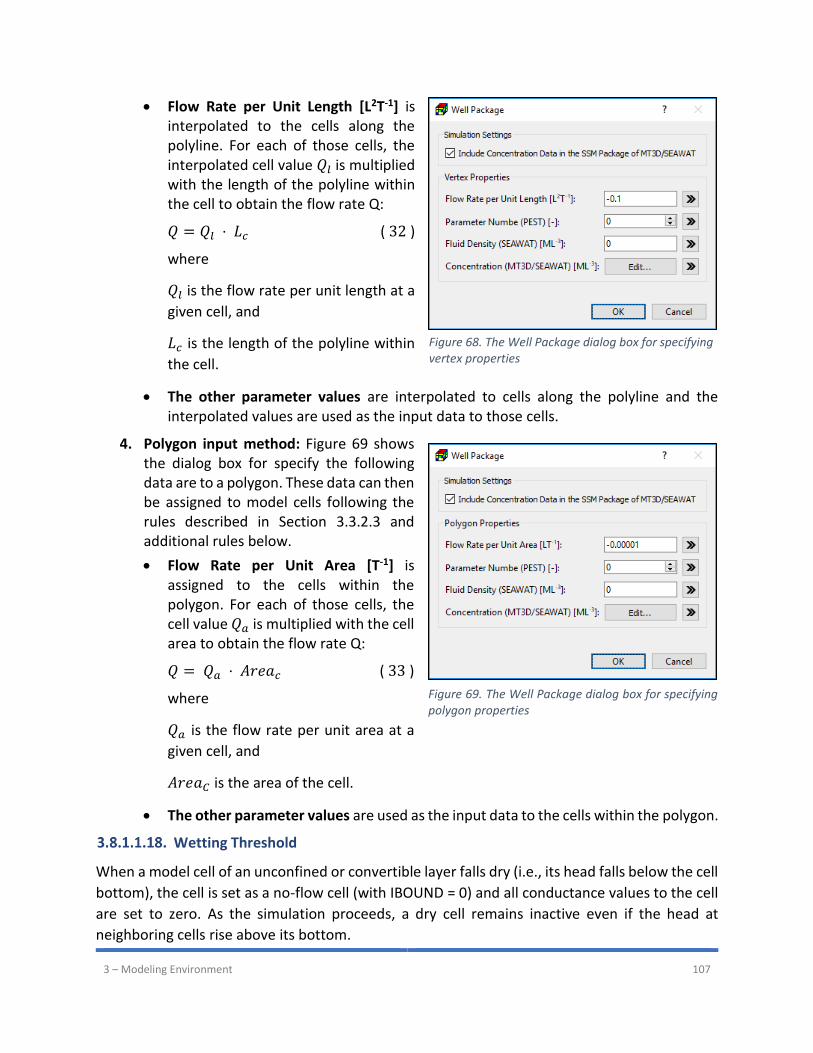
3 – Modeling Environment 107
• Flow Rate per Unit Length [L2T-1] is interpolated to the cells along the polyline. For each of those cells, the interpolated cell value 𝑄𝑙 is multiplied with the length of the polyline within the cell to obtain the flow rate Q:
𝑄 = 𝑄𝑙 ⋅ 𝐿𝑐 ( 32 )
where
𝑄𝑙 is the flow rate per unit length at a
given cell, and
𝐿𝑐 is the length of the polyline within
the cell.
• The other parameter values are interpolated to cells along the polyline and the interpolated values are used as the input data to those cells.
4. Polygon input method: Figure 69 shows the dialog box for specify the following data are to a polygon. These data can then be assigned to model cells following the rules described in Section 3.3.2.3 and additional rules below.
• Flow Rate per Unit Area [T-1] is assigned to the cells within the polygon. For each of those cells, the cell value 𝑄𝑎 is multiplied with the cell area to obtain the flow rate Q:
𝑄 = 𝑄𝑎 ⋅ 𝐴𝑟𝑒𝑎𝑐 ( 33 )
where
𝑄𝑎 is the flow rate per unit area at a
given cell, and
𝐴𝑟𝑒𝑎𝐶 is the area of the cell.
• The other parameter values are used as the input data to the cells within the polygon.
Wetting Threshold
When a model cell of an unconfined or convertible layer falls dry (i.e., its head falls below the cell
bottom), the cell is set as a no-flow cell (with IBOUND = 0) and all conductance values to the cell
are set to zero. As the simulation proceeds, a dry cell remains inactive even if the head at
neighboring cells rise above its bottom.
Figure 68. The Well Package dialog box for specifying vertex properties
Figure 69. The Well Package dialog box for specifying polygon properties
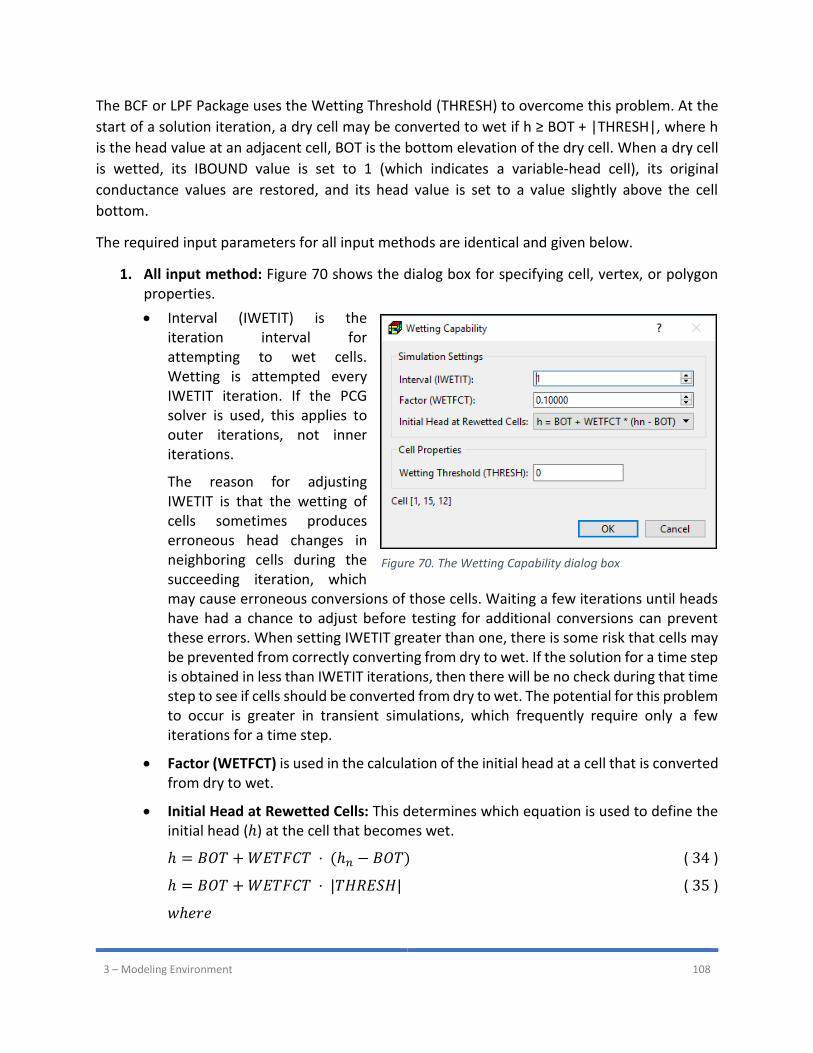
3 – Modeling Environment 108
The BCF or LPF Package uses the Wetting Threshold (THRESH) to overcome this problem. At the
start of a solution iteration, a dry cell may be converted to wet if h ≥ BOT + |THRESH|, where h
is the head value at an adjacent cell, BOT is the bottom elevation of the dry cell. When a dry cell
is wetted, its IBOUND value is set to 1 (which indicates a variable-head cell), its original
conductance values are restored, and its head value is set to a value slightly above the cell
bottom.
The required input parameters for all input methods are identical and given below.
1. All input method: Figure 70 shows the dialog box for specifying cell, vertex, or polygon properties.
• Interval (IWETIT) is the iteration interval for attempting to wet cells. Wetting is attempted every IWETIT iteration. If the PCG solver is used, this applies to outer iterations, not inner iterations.
The reason for adjusting IWETIT is that the wetting of cells sometimes produces erroneous head changes in neighboring cells during the succeeding iteration, which may cause erroneous conversions of those cells. Waiting a few iterations until heads have had a chance to adjust before testing for additional conversions can prevent these errors. When setting IWETIT greater than one, there is some risk that cells may be prevented from correctly converting from dry to wet. If the solution for a time step is obtained in less than IWETIT iterations, then there will be no check during that time step to see if cells should be converted from dry to wet. The potential for this problem to occur is greater in transient simulations, which frequently require only a few iterations for a time step.
• Factor (WETFCT) is used in the calculation of the initial head at a cell that is converted from dry to wet.
• Initial Head at Rewetted Cells: This determines which equation is used to define the initial head (ℎ) at the cell that becomes wet.
ℎ = 𝐵𝑂𝑇 + 𝑊𝐸𝑇𝐹𝐶𝑇 ⋅ (ℎ𝑛 − 𝐵𝑂𝑇) ( 34 )
ℎ = 𝐵𝑂𝑇 + 𝑊𝐸𝑇𝐹𝐶𝑇 ⋅ |𝑇𝐻𝑅𝐸𝑆𝐻| ( 35 )
𝑤ℎ𝑒𝑟𝑒
Figure 70. The Wetting Capability dialog box
3 – Modeling Environment 109
𝐵𝑂𝑇 is the bottom elevation of the cell,
ℎ𝑛 is the head at an adjacent cell, and
|𝑇𝐻𝑅𝐸𝑆𝐻| is the absolute value of the wetting threshold at the cell.
The initial estimate of head at a cell that converts to wet is theoretically unimportant because the solver should calculate the correct value in subsequent iterations. In practice, however, the initial estimate is often important for solver efficiency; that is, if a poor choice is made, the solver convergence may be slower than optimum. A bad choice for initial head also can cause the cell to oscillate between wet and dry.
• Wetting Threshold (THRESH): When the head at an adjacent cell equals or exceeds BOT + |THRESH| of a dry cell, the dry cell is wetted. The sign of THRESH is used as a flag:
o If THRESH < 0, only the cell below a dry cell can cause the cell to become wet.
o If THRESH > 0, the cell below a dry cell and the four horizontally adjacent cells can
cause a cell to become wet.
o If THRESH is 0, the cell cannot be wetted.
A primary difficulty with the rewetting approach is that the value of THRESH must be determined by trial and error. If |THRESH| is too low, a cell may be incorrectly converted to wet. That is, a cell may convert to wet and then reconvert to dry in later solver iterations because the head does not stay above the bottom elevation. This cycle of converting between wet and dry conditions can repeat indefinitely, preventing the solver from converging. Larger values of |THRESH| can avoid repeated conversion between wet and dry, but they increase the non-uniqueness of the solution (McDonald, et al., 1991).
The method of wetting and drying cells used in the BCF and LPF Packages can cause convergence
problems with the iterative solvers. Symptoms of a convergence problem are slow convergence
or divergence combined with the frequent wetting and drying of the same cells. For example, a
well-cell with large pumping rate could cause the cell (and perhaps also neighboring cells) to fall
dry. Thus, the pumping at that cell is switched off, the water table rises due to lack of pumping,
the dry cell is wetted, and the pumping is re-established. The cycle repeats. Similar problems may
occur near sinks or at places with small saturated thickness. You can detect such situations by
examining the model run listing file with Models > MODFLOW > View > Run Listing File. A message
is printed to that file each time a cell converts. Some options to mitigate the convergence
problems are
1. Modify the settings
• Set THRESH < 0, so that wetting can only be from below.
• Increase IWETIT.
• Use another equation for calculating the initial head at rewetted cells.
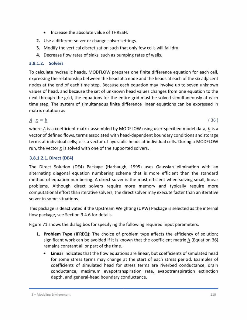
3 – Modeling Environment 110
• Increase the absolute value of THRESH.
2. Use a different solver or change solver settings.
3. Modify the vertical discretization such that only few cells will fall dry.
4. Decrease flow rates of sinks, such as pumping rates of wells.
3.8.1.2. Solvers
To calculate hydraulic heads, MODFLOW prepares one finite difference equation for each cell,
expressing the relationship between the head at a node and the heads at each of the six adjacent
nodes at the end of each time step. Because each equation may involve up to seven unknown
values of head, and because the set of unknown head values changes from one equation to the
next through the grid, the equations for the entire grid must be solved simultaneously at each
time step. The system of simultaneous finite difference linear equations can be expressed in
matrix notation as
𝐴 ∙ 𝑥 = 𝑏 ( 36 )
where 𝐴 is a coefficient matrix assembled by MODFLOW using user-specified model data; 𝑏 is a
vector of defined flows, terms associated with head-dependent boundary conditions and storage
terms at individual cells; 𝑥 is a vector of hydraulic heads at individual cells. During a MODFLOW
run, the vector 𝑥 is solved with one of the supported solvers.
Direct (DE4)
The Direct Solution (DE4) Package (Harbaugh, 1995) uses Gaussian elimination with an
alternating diagonal equation numbering scheme that is more efficient than the standard
method of equation numbering. A direct solver is the most efficient when solving small, linear
problems. Although direct solvers require more memory and typically require more
computational effort than iterative solvers, the direct solver may execute faster than an iterative
solver in some situations.
This package is deactivated if the Upstream Weighting (UPW) Package is selected as the internal
flow package, see Section 3.4.6 for details.
Figure 71 shows the dialog box for specifying the following required input parameters:
1. Problem Type (IFREQ): The choice of problem type affects the efficiency of solution; significant work can be avoided if it is known that the coefficient matrix A (Equation 36)
remains constant all or part of the time.
• Linear indicates that the flow equations are linear, but coefficients of simulated head for some stress terms may change at the start of each stress period. Examples of coefficients of simulated head for stress terms are riverbed conductance, drain conductance, maximum evapotranspiration rate, evapotranspiration extinction depth, and general-head boundary conductance.
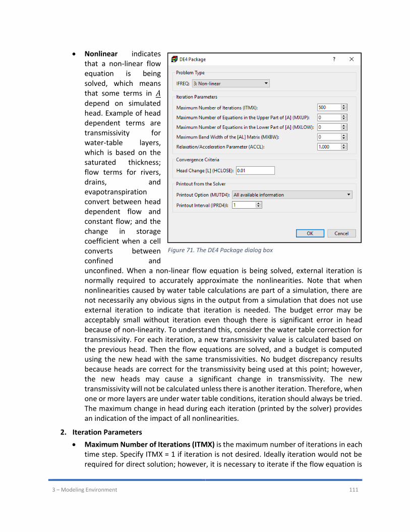
3 – Modeling Environment 111
• Nonlinear indicates that a non-linear flow equation is being solved, which means that some terms in 𝐴 depend on simulated head. Example of head dependent terms are transmissivity for water-table layers, which is based on the saturated thickness; flow terms for rivers, drains, and evapotranspiration convert between head dependent flow and constant flow; and the change in storage coefficient when a cell converts between confined and unconfined. When a non-linear flow equation is being solved, external iteration is normally required to accurately approximate the nonlinearities. Note that when nonlinearities caused by water table calculations are part of a simulation, there are not necessarily any obvious signs in the output from a simulation that does not use external iteration to indicate that iteration is needed. The budget error may be acceptably small without iteration even though there is significant error in head because of non-linearity. To understand this, consider the water table correction for transmissivity. For each iteration, a new transmissivity value is calculated based on the previous head. Then the flow equations are solved, and a budget is computed using the new head with the same transmissivities. No budget discrepancy results because heads are correct for the transmissivity being used at this point; however, the new heads may cause a significant change in transmissivity. The new transmissivity will not be calculated unless there is another iteration. Therefore, when one or more layers are under water table conditions, iteration should always be tried. The maximum change in head during each iteration (printed by the solver) provides an indication of the impact of all nonlinearities.
2. Iteration Parameters
• Maximum Number of Iterations (ITMX) is the maximum number of iterations in each time step. Specify ITMX = 1 if iteration is not desired. Ideally iteration would not be required for direct solution; however, it is necessary to iterate if the flow equation is
Figure 71. The DE4 Package dialog box
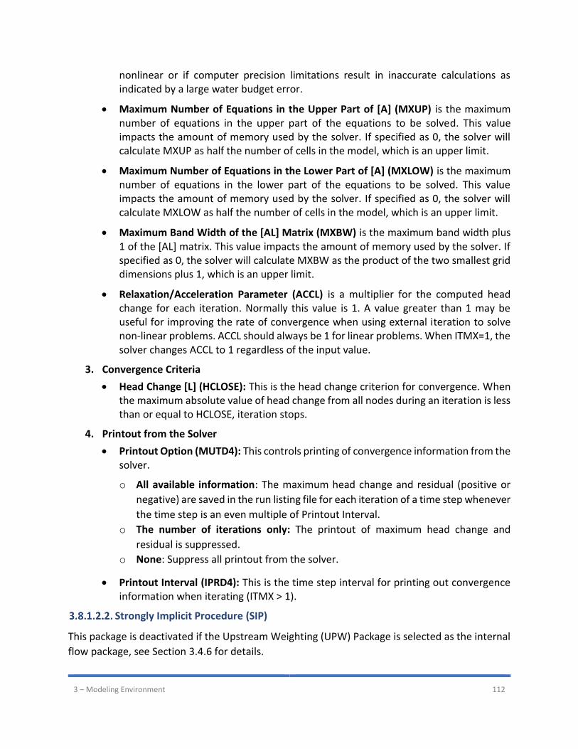
3 – Modeling Environment 112
nonlinear or if computer precision limitations result in inaccurate calculations as indicated by a large water budget error.
• Maximum Number of Equations in the Upper Part of [A] (MXUP) is the maximum number of equations in the upper part of the equations to be solved. This value impacts the amount of memory used by the solver. If specified as 0, the solver will calculate MXUP as half the number of cells in the model, which is an upper limit.
• Maximum Number of Equations in the Lower Part of [A] (MXLOW) is the maximum number of equations in the lower part of the equations to be solved. This value impacts the amount of memory used by the solver. If specified as 0, the solver will calculate MXLOW as half the number of cells in the model, which is an upper limit.
• Maximum Band Width of the [AL] Matrix (MXBW) is the maximum band width plus 1 of the [AL] matrix. This value impacts the amount of memory used by the solver. If specified as 0, the solver will calculate MXBW as the product of the two smallest grid dimensions plus 1, which is an upper limit.
• Relaxation/Acceleration Parameter (ACCL) is a multiplier for the computed head change for each iteration. Normally this value is 1. A value greater than 1 may be useful for improving the rate of convergence when using external iteration to solve non-linear problems. ACCL should always be 1 for linear problems. When ITMX=1, the solver changes ACCL to 1 regardless of the input value.
3. Convergence Criteria
• Head Change [L] (HCLOSE): This is the head change criterion for convergence. When the maximum absolute value of head change from all nodes during an iteration is less than or equal to HCLOSE, iteration stops.
4. Printout from the Solver
• Printout Option (MUTD4): This controls printing of convergence information from the solver.
o All available information: The maximum head change and residual (positive or
negative) are saved in the run listing file for each iteration of a time step whenever
the time step is an even multiple of Printout Interval.
o The number of iterations only: The printout of maximum head change and
residual is suppressed.
o None: Suppress all printout from the solver.
• Printout Interval (IPRD4): This is the time step interval for printing out convergence information when iterating (ITMX > 1).
Strongly Implicit Procedure (SIP)
This package is deactivated if the Upstream Weighting (UPW) Package is selected as the internal
flow package, see Section 3.4.6 for details.

3 – Modeling Environment 113
Figure 72 shows the dialog box for specifying the
following required input parameters:
1. Iteration Parameters
• Maximum Number of Iterations (MXITER) is the maximum number of times through the iteration loop in one time step to solve the system of equations.
• Number of Iteration Parameters (NPARM) is the number of iteration variables to be used. Five variables are generally sufficient.
• Acceleration Parameter (ACCL) is the acceleration variable. It must be greater than zero and is generally equal to one. If a zero is entered, it is changed to one by the solver.
2. Convergence Criteria
• Head Change (HCLOSE) [L]: This is the head change criterion for convergence. When the maximum absolute value of head change from all nodes during an iteration is less than or equal to HCLOSE, iteration stops.
3. Printout from the Solver
• Printout Interval (IPRSIP): The maximum head change (positive or negative) is printed for each iteration of a time step whenever the time step is an even multiple of IPRSIP.
Geometric Multigrid (GMG)
This package is deactivated if the Upstream Weighting (UPW) Package is selected as the internal
flow package, see Section 3.4.6 for details.
Figure 73 shows the dialog box for specifying the following required input parameters of the
Geometric Multigrid Solver (GMG) Package (Wilson, et al., 2004).
1. Preconditioning Method
• Smoother Type (ISM): ISM controls the type of smoother used in the multigrid preconditioner.
o ILU Smoothing: Select this option to implement ILU(0) smoothing in the multigrid
preconditioner. This smoothing requires an additional vector on each multigrid
level to store the pivots in the ILU factorization.
o Symmetric Gauss-Seidel (SGS) Smoothing: Select this option to implement the
Symmetric Gauss-Seidel (SGS) smoothing in the multigrid preconditioner. No
additional storage is required for this smoother; users may want to use this option
Figure 72. The SIP Package dialog box
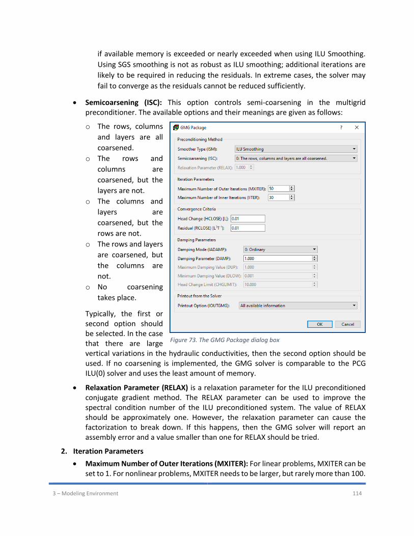
3 – Modeling Environment 114
if available memory is exceeded or nearly exceeded when using ILU Smoothing.
Using SGS smoothing is not as robust as ILU smoothing; additional iterations are
likely to be required in reducing the residuals. In extreme cases, the solver may
fail to converge as the residuals cannot be reduced sufficiently.
• Semicoarsening (ISC): This option controls semi-coarsening in the multigrid preconditioner. The available options and their meanings are given as follows:
o The rows, columns
and layers are all
coarsened.
o The rows and
columns are
coarsened, but the
layers are not.
o The columns and
layers are
coarsened, but the
rows are not.
o The rows and layers
are coarsened, but
the columns are
not.
o No coarsening
takes place.
Typically, the first or second option should be selected. In the case that there are large vertical variations in the hydraulic conductivities, then the second option should be used. If no coarsening is implemented, the GMG solver is comparable to the PCG ILU(0) solver and uses the least amount of memory.
• Relaxation Parameter (RELAX) is a relaxation parameter for the ILU preconditioned conjugate gradient method. The RELAX parameter can be used to improve the spectral condition number of the ILU preconditioned system. The value of RELAX should be approximately one. However, the relaxation parameter can cause the factorization to break down. If this happens, then the GMG solver will report an assembly error and a value smaller than one for RELAX should be tried.
2. Iteration Parameters
• Maximum Number of Outer Iterations (MXITER): For linear problems, MXITER can be set to 1. For nonlinear problems, MXITER needs to be larger, but rarely more than 100.
Figure 73. The GMG Package dialog box
3 – Modeling Environment 115
• Maximum Number of Inner Iterations (IITER) is the maximum number of PCG iterations for each linear solution. A value of 100 is typically sufficient. It is frequently useful to specify a smaller number for nonlinear problems to prevent an excessive number of inner iterations.
3. Convergence Criteria
• Head Change (HCLOSE) [L] is the head change convergence criterion for nonlinear problems. After each linear solve (inner iteration), the maximum of the head change is compared against HCLOSE. HCLOSE can be set to a large number for linear problems; HCLOSE is ignored if MXITER=1.
• Residual (RCLOSE) [L3T-1] is the residual convergence criterion for the inner iteration. Typically, RCLOSE is set to the same value as HCLOSE. If RCLOSE is set too high, then additional outer iterations may be required due to the linear equation not being solved with sufficient accuracy. On the other hand, a too restrictive setting for RCLOSE for nonlinear problems may force an unnecessarily accurate linear solution.
4. Damping Parameters
• Damping Mode (IADAMP) is a flag that controls adaptive damping. The possible values of IADAMP and their meanings are as follows:
o 0: Ordinary: the value assigned to DAMP is used as a constant damping parameter.
o 1: Cooley’s method: the value of DAMP is used for the first nonlinear iteration.
The damping parameter is adaptively varied based on the head change, using
Cooley’s method as described in (Mehl, et al., 2001), for subsequent iterations.
o 2. Relative reduced residual method: the relative reduced residual damping
method documented in (Mehl, et al., 2001) and modified by (Banta, 2006) is used.
When IADAMP is specified as 2 and the value specified for DAMP is less than 0.5, the closure criterion for the inner iterations (DRCLOSE) is assigned simply as RCLOSE. When DAMP is between 0.5 and 1.0, inclusive, or when IADAMP is specified as 0 or 1, DRCLOSE is calculated according to equation 20 on p. 9 of (Wilson, et al., 2004)
• Damping Parameter (DAMP) is the value of the damping parameter. For linear problems, a value of 1.0 should be used. For nonlinear problems, a value less than 1.0 but greater than 0.0 may be necessary to achieve convergence. A typical value for nonlinear problems is 0.5. Damping also helps control the convergence criterion of the linear solve to alleviate excessive PCG iterations.
• Maximum Damping Value (DUP) is the maximum damping value that should be applied at any iteration when the solver is not oscillating; it is dimensionless. An appropriate value for DUP will be problem-dependent. For moderately nonlinear problems, reasonable values for DUP would be in the range 0.5 to 1.0. For a highly nonlinear problem, a reasonable value for DUP could be as small as 0.1. When the solver is oscillating, a damping value as large as 2.0 × DUP may be applied.
3 – Modeling Environment 116
• Minimum Damping Value (DLOW) is the minimum damping value to be generated by the adaptive-damping procedure; it is dimensionless. An appropriate value for DLOW will be problem-dependent and will be smaller than the value specified for DUP. For a highly nonlinear problem, an appropriate value for DLOW might be as small as 0.001.
• Head Change Limit (CHGLIMIT) is the maximum allowed head change at any cell between outer iterations.
5. Printout from the Solver
• Printout Option (IOUTGMG): This controls printing of convergence information from the solver. Available options are
o Only the solver inputs
o All available information
o The convergence history of the PCG iteration
Preconditioned Conjugate Gradient (PCG)
The Preconditioned Conjugate-Gradient Solver (PCG) Package is fully documented in (Hill, 1990).
The PCG solver incorporates two forms of the Preconditioned Conjugate-Gradient method: the
Modified Incomplete Cholesky and the Polynomial methods. Knowledge of the details of these
methods generally is not necessary. The most important aspect is that the Modified Incomplete
Cholesky method is almost always faster. The Polynomial method is potentially faster only on
parallel computers where some of the work can be performed simultaneously on multiple
processors.
This package is deactivated if the Upstream Weighting (UPW) Package is selected as the internal
flow package, see Section 3.4.6 for details.
Figure 74 shows the dialog box for specifying the following required input parameters:
1. Preconditioning Method
• NPCOND: This is the matrix preconditioning method. The available options are
o Modified Incomplete Cholesky (for use on scalar computers)
o Neuman series polynomial (for use on parallel computers)
• NBPOL: This is used with the Neuman series polynomial preconditioning method. Checking this box to calculate the estimate of the upper bound on the maximum eigenvalue. If this box is cleared, the estimate is set as 2. Convergence is generally insensitive to this parameter.
2. Iteration Parameters
• Maximum Number of Outer Iterations (MXITER): For a linear problem MXITER should be 1, unless more than 50 inner iterations are required, when MXITER could be as large as 10. A larger number (generally less than 100) is required for a nonlinear problem.
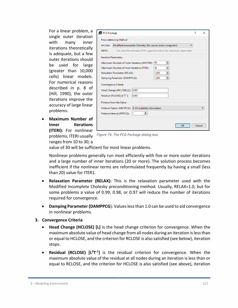
3 – Modeling Environment 117
For a linear problem, a single outer iteration with many inner iterations theoretically is adequate, but a few outer iterations should be used for large (greater than 10,000 cells) linear models. For numerical reasons described in p. 8 of (Hill, 1990), the outer iterations improve the accuracy of large linear problems.
• Maximum Number of Inner Iterations (ITERI): For nonlinear problems, ITERI usually ranges from 10 to 30; a value of 30 will be sufficient for most linear problems.
Nonlinear problems generally run most efficiently with five or more outer iterations and a large number of inner iterations (20 or more). The solution process becomes inefficient if the nonlinear terms are reformulated frequently by having a small (less than 20) value for ITER1.
• Relaxation Parameter (RELAX): This is the relaxation parameter used with the Modified Incomplete Cholesky preconditioning method. Usually, RELAX=1.0, but for some problems a value of 0.99, 0.98, or 0.97 will reduce the number of iterations required for convergence.
• Damping Parameter (DAMPPCG): Values less than 1.0 can be used to aid convergence in nonlinear problems.
3. Convergence Criteria
• Head Change (HCLOSE) [L] is the head change criterion for convergence. When the maximum absolute value of head change from all nodes during an iteration is less than or equal to HCLOSE, and the criterion for RCLOSE is also satisfied (see below), iteration stops.
• Residual (RCLOSE) [L3T-1] is the residual criterion for convergence. When the maximum absolute value of the residual at all nodes during an iteration is less than or equal to RCLOSE, and the criterion for HCLOSE is also satisfied (see above), iteration
Figure 74. The PCG Package dialog box
3 – Modeling Environment 118
stops. For nonlinear problems, convergence is achieved when the convergence criteria are satisfied for the first inner iteration.
4. Printout from the Solver
• Printout Option (MUTPCG) is a flag that controls printing of convergence information from the solver:
o 0: All available information: Print tables of maximum head change and residual
each iteration.
o 1: The number of iterations only: Print only the total number of iterations
o 2: None: No Printing.
o 3: Print as for 0, but only if solver convergence fails
• Printout Interval (IPRPCG): The extreme head change and residual (positive or negative) are printed for each iteration of a time step whenever the time step is an even multiple of the printout interval. The printout also occurs at the end of each stress period regardless of the value of the printout interval.
PCG with Improved Nonlinear Control (PCGN)
The principal objective of the preconditioned conjugate gradient with improved nonlinear control
(PCGN) Package (Naff, et al., 2008) is to provide the modeler with more options when faced with
a poorly converging nonlinear problem. Picard iteration is used to solve nonlinear ground-water
flow equations by iteratively solving a linear approximation of the nonlinear equations. The linear
solution is provided by means of the preconditioned conjugate gradient algorithm where
preconditioning is provided by the modified incomplete Cholesky algorithm. The incomplete
Cholesky scheme incorporates two levels of fill, 0 and 1, in which the pivots can be modified so
that the row sums of the preconditioning matrix and the original matrix are approximately equal.
A relaxation factor is used to implement the modified pivots, which determines the degree of
modification allowed. The preconditioned conjugate gradient method is coupled with Picard
iteration to efficiently solve the nonlinear equations associated with many ground-water flow
problems.
This package is deactivated if the Upstream Weighting (UPW) Package is selected as the internal
flow package, see Section 3.4.6 for details.
Figure 75 shows the dialog box for specifying the following required input parameters:
1. Iteration Parameters
• Maximum Number of Outer Iterations (ITER_MO): For nonlinear problems, this variable must be set to some number greater than one, depending on the problem size and degree of nonlinearity. If this variable is set to 1, then the PCGN solver assumes that the problem is linear.
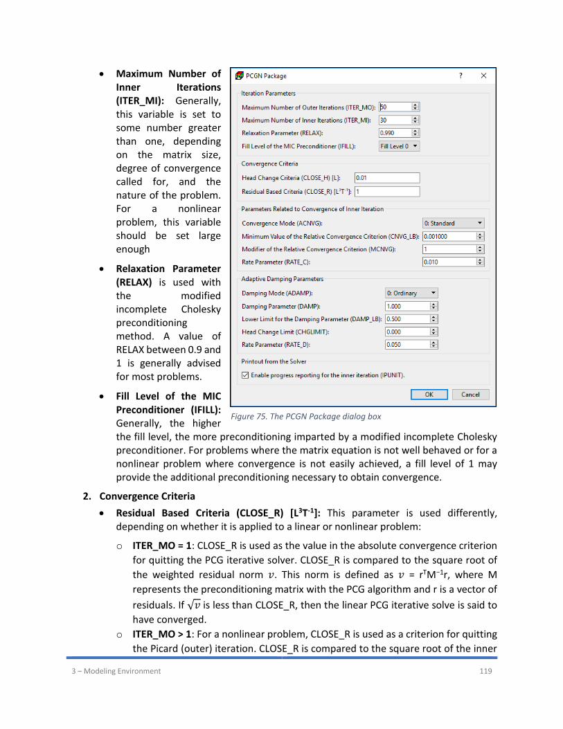
3 – Modeling Environment 119
• Maximum Number of Inner Iterations (ITER_MI): Generally, this variable is set to some number greater than one, depending on the matrix size, degree of convergence called for, and the nature of the problem. For a nonlinear problem, this variable should be set large enough
• Relaxation Parameter (RELAX) is used with the modified incomplete Cholesky preconditioning method. A value of RELAX between 0.9 and 1 is generally advised for most problems.
• Fill Level of the MIC Preconditioner (IFILL): Generally, the higher the fill level, the more preconditioning imparted by a modified incomplete Cholesky preconditioner. For problems where the matrix equation is not well behaved or for a nonlinear problem where convergence is not easily achieved, a fill level of 1 may provide the additional preconditioning necessary to obtain convergence.
2. Convergence Criteria
• Residual Based Criteria (CLOSE_R) [L3T-1]: This parameter is used differently, depending on whether it is applied to a linear or nonlinear problem:
o ITER_MO = 1: CLOSE_R is used as the value in the absolute convergence criterion
for quitting the PCG iterative solver. CLOSE_R is compared to the square root of
the weighted residual norm 𝑣. This norm is defined as 𝑣 = rTM−1r, where M
represents the preconditioning matrix with the PCG algorithm and r is a vector of
residuals. If √𝑣 is less than CLOSE_R, then the linear PCG iterative solve is said to
have converged.
o ITER_MO > 1: For a nonlinear problem, CLOSE_R is used as a criterion for quitting
the Picard (outer) iteration. CLOSE_R is compared to the square root of the inner
Figure 75. The PCGN Package dialog box
3 – Modeling Environment 120
product of the residuals (the residual norm), [rTr]1/2, as calculated on entry to the
PCG solver at the beginning of every Picard iteration. If this norm is less than
CLOSE_R, then the Picard iteration is considered to have converged.
• Head Change Criteria (CLOSE_H) [L]: CLOSE_H is used as an alternate stopping criterion for the Picard iteration needed to solve a nonlinear problem. The maximum value of the head change is obtained for each Picard iteration, after completion of the inner, PCG iteration. If this maximum head change is less than CLOSE_H, then the Picard iteration is considered tentatively to have converged. However, as nonlinear problems can demonstrate oscillation in the head solution, the Picard iteration is not declared to have converged unless the maximum head change is less than CLOSE_H for three Picard iterations. If these Picard iterations are sequential, then a good solution is assumed to have been obtained. If the Picard iterations are not sequential, then a warning is issued advising that the convergence is conditional and the user is urged to examine the mass balance of the solution.
3. Parameters Related to Convergence of Inner Iteration
• Convergence Mode (ACNVG): ACNVG defines the mode of convergence applied to the PCG solver. In general, the relative stopping criterion for PCG iteration is 𝑣𝑖 < 𝜀𝑣0 where 𝑣0 is the weighted residual norm on entry to the PCG solver, 𝜀 is the relative convergence parameter, and 𝑣𝑖 is the same norm at PCG iteration i. The available convergence modes are:
o ACNVG=0: The standard convergence scheme is employed. The standard relative
convergence is denoted by 𝜀𝑠 and usually takes the value 0.1; this value is assigned
to the relative convergence 𝜀. No additional variables are used.
o ACNVG=1: Adaptive convergence is employed. The adaptive convergence scheme
adjusts the relative convergence 𝜀 of the PCG iteration based on a measure of the
nonlinearity of the problem. Under this scheme, 𝜀 is allowed to vary such that
CNVG_LB < 𝜀 < 𝜀𝑠 where the exact value of 𝜀 is dependent on the measure of
nonlinearity. This option requires a valid value for variable CNVG_LB.
o ACNVG=2: Enhanced convergence is employed. If the variable enhancement
option is employed (RATE_C > 0), then 𝜀𝑠 is taken as the upper limit for 𝜀. This
option requires valid values for variables MCNVG and RATE_C.
• Minimum Value of the Relative Convergence Criterion (CNVG_LB) is used only in convergence mode ACNVG = 1. CNVG_LB is the minimum value that the relative convergence 𝜀 can take under the self-adjusting convergence option. The objective here is to prevent 𝜀 from becoming so small that the PCG solver takes an excessive number of iterations. Valid range for variable: 0 < CNVG_LB < 𝜀𝑠; a value of CNVG_LB = 0.001 usually produces reasonable results.
• Modifier of the Relative Convergence Criterion (MCNVG) is used only in convergence mode ACNVG = 2. MCNVG increases the relative PCG convergence criteria by a power
3 – Modeling Environment 121
equal to MCNVG; that is, letting p = MCNVG, then the relative convergence criterion
ε is enhanced such that 𝜀 = 𝜀𝑠𝑝 where 0 < 𝑝 ≤ 6. If MCNVG is set to a value greater
than 6, then PCGN resets MCNVG = 6 and issues a warning message. If RATE_C = 0, then this enhanced relative convergence criterion is applied uniformly throughout the simulation; the relative convergence, in this case, is not adjusted for stress changes in the simulation. MCNVG must be set to a value greater than zero when ACNVG = 2; otherwise a data error is declared and ACNVG is reset to zero.
• Rate Parameter (RATE_C) is used only in convergence mode ACNVG = 2; this option results in variable enhancement of 𝜀. If 0 < RATE_C < 1, then enhanced relative convergence is allowed to decrease by increasing 𝜀 as follows: 𝜀𝑗 = 𝜀𝑗−1 + 𝑅𝐴𝑇𝐸_𝐶 ∙
𝜀𝑗−1 where j is the Picard iteration number; this change in 𝜀 occurs so long as the
Picard iteration progresses satisfactorily. If RATE_C ≤ 0, then the value of 𝜀 set by MCNVG remains unchanged through the Picard iteration. It should be emphasized that RATE_C must have a value greater than 0 for the variable enhancement to be effective; otherwise 𝜀 remains constant. The assumption here is that a better solution of the linear equations is needed initially to improve the nonlinear Picard solution, but that this need abates with additional Picard iterations. Typical values for RATE_C are 0.01 < RATE_C < 0.1, although larger or smaller values may be used.
4. Adaptive Damping Parameters
• Damping Mode (ADAMP) defines the mode of damping applied to the linear solution. In general, damping determines how much of the head changes vector Δj shall be applied to the hydraulic head vector hj in Picard iteration j: ℎ𝑗 = ℎ𝑗−1 + 𝜃Δ𝑗, where θ
is the damping parameter. The available damping modes are:
o ADAMP = 0: Ordinary damping is employed and a constant value of damping
parameter θ = DAMP will be used throughout the Picard iteration. This option
requires a valid value for DAMP.
o ADAMP = 1: Adaptive damping is employed; Adaptive damping changes the
damping parameter θ in response to the difficulty the nonlinear solver encounters
in solving a given problem. Essentially, the nonlinear solver looks to increase θ
should the convergence of the Picard iteration proceed satisfactorily, but
otherwise causes θ to decrease. Adaptive damping can be useful for problems that
do not converge readily, but otherwise should be avoided as it generally requires
more total iterations. This option requires valid values for variables DAMP,
DAMP_LB, RATE_D, and CHGLIMIT. Adaptive damping also admits the possibility
of directly limiting the maximum head change applicable to update the hydraulic
heads; see CHGLIMIT below. If this option is not desired, then CHGLIMIT should
be set to zero.
o ADAMP = 2: Enhanced damping algorithm in which the value of θ is increased (but
never decreased) provided the Picard iteration is proceeding satisfactorily. This
enhanced damping allows θ to increase from a minimum value to a maximum
3 – Modeling Environment 122
value DAMP by a rate equal to RATE_D. The minimum value in the first stress
period is DAMP_LB; for subsequent stress periods, it is the geometric mean of
DAMP and DAMP_LB. This option requires valid values for DAMP, DAMP_LB, and
RATE_D.
• Damping Parameter (DAMP) restricts the damping parameter θ; generally, 0 < DAMP < 1. Its function for the various modes of ADAMP are:
o ADAMP = 0: The damping parameter θ takes on the value DAMP and is maintained
constant throughout the simulation.
o ADAMP > 0: The value of DAMP will be treated as the upper limit for θ in the
enhanced damping or adaptive damping algorithms.
• Lower Limit for the Damping Parameter (DAMP_LB) represents a bound placed on θ; generally, 0 < DAMP_LB < DAMP. For the various modes of ADAMP > 0, DAMP_LB serves the following purposes:
o ADAMP = 1: In the adaptive damping algorithm, DAMP_LB represents the lower
limit to which θ, under adverse adaptive damping conditions, will be allowed to
fall.
o ADAMP = 2: In the enhanced damping algorithm, DAMP_LB is the starting value
(or a component of the starting value) for the damping parameter θ used in the
initial Picard iteration of every stress period.
• Head Change Limit (CHGLIMIT) limits the maximum head change applicable to the updated hydraulic heads in a Picard iteration. Provided that the current damping factor is greater than the ratio of CHGLIMIT to the maximum head change and that this ratio is less than one, then the damping factor is reset to the value of the ratio. This option is available only in association with adaptive damping: ACNVG = 1. If CHGLIMIT = 0.0, then adaptive damping proceeds without this feature.
• Rate Parameter (RATE_D): Generally, 0 < RATE_D < 1. For the various modes of ADAMP > 0, RATE_D serves the following purposes:
o ADAMP = 1: RATE_D sets the recovery rate for the damping factor θ in response
to the progress in the Picard iteration; it also forms a limit on the response
function to progress in the Picard iteration. Typical values for RATE_D, under this
scenario, are 0.01 < RATE_D < 0.1. Under adaptive damping, if the user finds that
the damping factor θ increases too rapidly, then reducing RATE_D will slow the
rate of increase.
o ADAMP = 2: Provided the Picard iteration is progressing satisfactorily, RATE_D
adjusts the damping factor θ upward such that 𝜃𝑗 = 𝜃𝑗−1 + 𝑅𝐴𝑇𝐸_𝐷 ∙ 𝜃𝑗−1,
where j is the Picard iteration number. Typical values for RATE_D, under this
scenario, are 0.01 < RATE_D < 0.1, although larger or smaller values may be used.
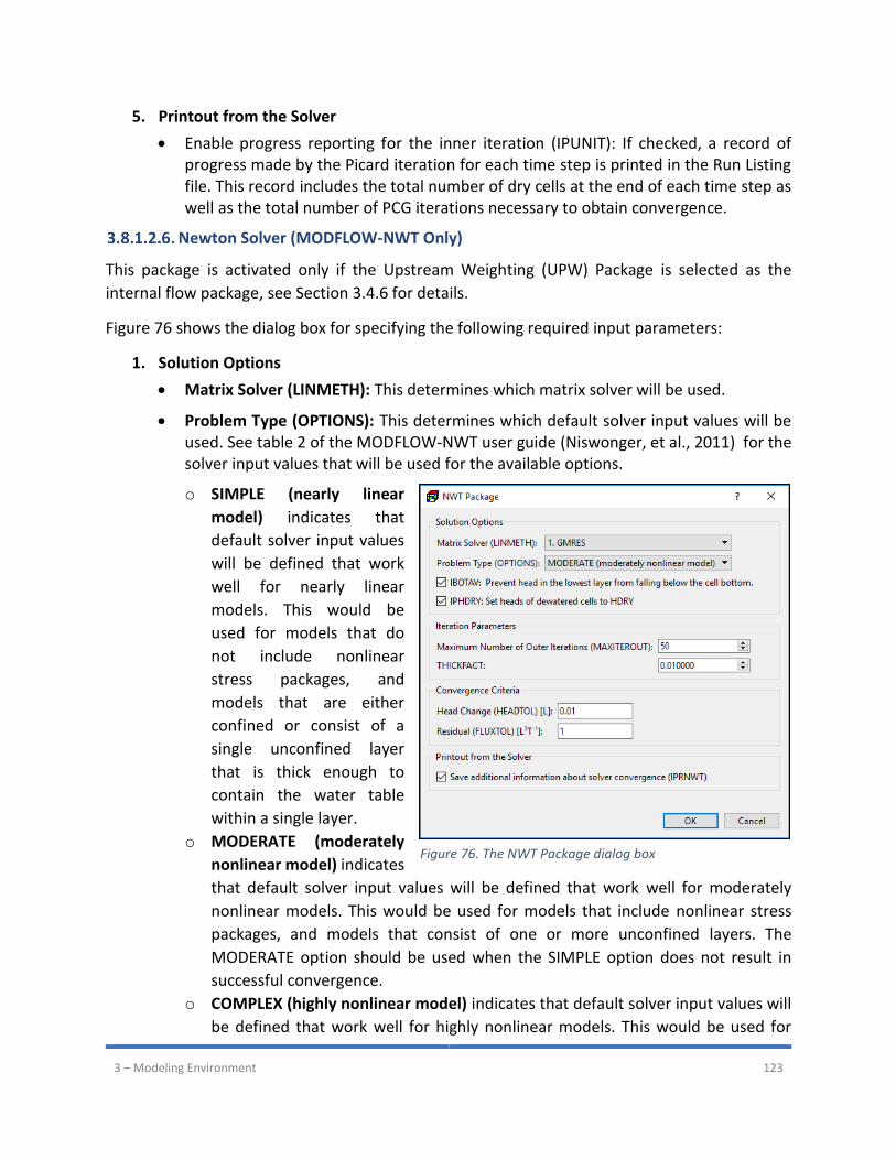
3 – Modeling Environment 123
5. Printout from the Solver
• Enable progress reporting for the inner iteration (IPUNIT): If checked, a record of progress made by the Picard iteration for each time step is printed in the Run Listing file. This record includes the total number of dry cells at the end of each time step as well as the total number of PCG iterations necessary to obtain convergence.
Newton Solver (MODFLOW-NWT Only)
This package is activated only if the Upstream Weighting (UPW) Package is selected as the
internal flow package, see Section 3.4.6 for details.
Figure 76 shows the dialog box for specifying the following required input parameters:
1. Solution Options
• Matrix Solver (LINMETH): This determines which matrix solver will be used.
• Problem Type (OPTIONS): This determines which default solver input values will be used. See table 2 of the MODFLOW-NWT user guide (Niswonger, et al., 2011) for the solver input values that will be used for the available options.
o SIMPLE (nearly linear
model) indicates that
default solver input values
will be defined that work
well for nearly linear
models. This would be
used for models that do
not include nonlinear
stress packages, and
models that are either
confined or consist of a
single unconfined layer
that is thick enough to
contain the water table
within a single layer.
o MODERATE (moderately
nonlinear model) indicates
that default solver input values will be defined that work well for moderately
nonlinear models. This would be used for models that include nonlinear stress
packages, and models that consist of one or more unconfined layers. The
MODERATE option should be used when the SIMPLE option does not result in
successful convergence.
o COMPLEX (highly nonlinear model) indicates that default solver input values will
be defined that work well for highly nonlinear models. This would be used for
Figure 76. The NWT Package dialog box
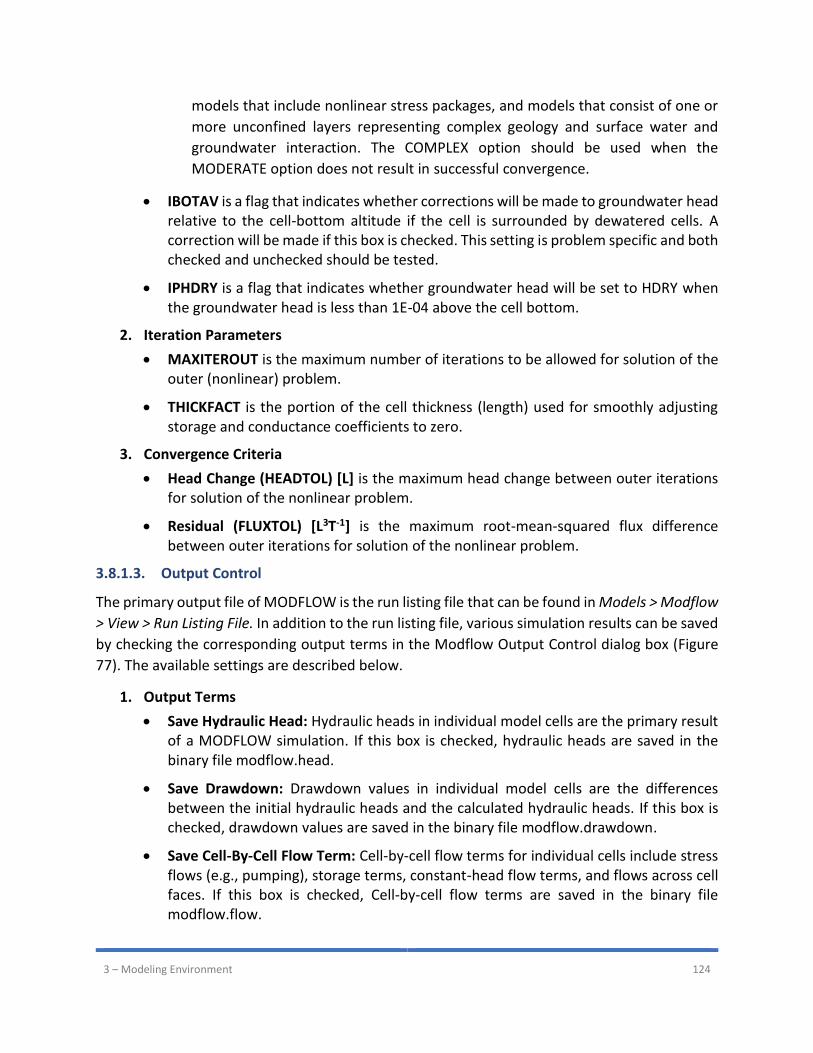
3 – Modeling Environment 124
models that include nonlinear stress packages, and models that consist of one or
more unconfined layers representing complex geology and surface water and
groundwater interaction. The COMPLEX option should be used when the
MODERATE option does not result in successful convergence.
• IBOTAV is a flag that indicates whether corrections will be made to groundwater head relative to the cell-bottom altitude if the cell is surrounded by dewatered cells. A correction will be made if this box is checked. This setting is problem specific and both checked and unchecked should be tested.
• IPHDRY is a flag that indicates whether groundwater head will be set to HDRY when the groundwater head is less than 1E-04 above the cell bottom.
2. Iteration Parameters
• MAXITEROUT is the maximum number of iterations to be allowed for solution of the outer (nonlinear) problem.
• THICKFACT is the portion of the cell thickness (length) used for smoothly adjusting storage and conductance coefficients to zero.
3. Convergence Criteria
• Head Change (HEADTOL) [L] is the maximum head change between outer iterations for solution of the nonlinear problem.
• Residual (FLUXTOL) [L3T-1] is the maximum root-mean-squared flux difference between outer iterations for solution of the nonlinear problem.
3.8.1.3. Output Control
The primary output file of MODFLOW is the run listing file that can be found in Models > Modflow
> View > Run Listing File. In addition to the run listing file, various simulation results can be saved
by checking the corresponding output terms in the Modflow Output Control dialog box (Figure
77). The available settings are described below.
1. Output Terms
• Save Hydraulic Head: Hydraulic heads in individual model cells are the primary result of a MODFLOW simulation. If this box is checked, hydraulic heads are saved in the binary file modflow.head.
• Save Drawdown: Drawdown values in individual model cells are the differences between the initial hydraulic heads and the calculated hydraulic heads. If this box is checked, drawdown values are saved in the binary file modflow.drawdown.
• Save Cell-By-Cell Flow Term: Cell-by-cell flow terms for individual cells include stress flows (e.g., pumping), storage terms, constant-head flow terms, and flows across cell faces. If this box is checked, Cell-by-cell flow terms are saved in the binary file modflow.flow.
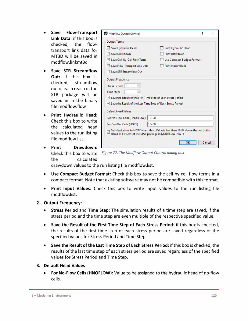
3 – Modeling Environment 125
• Save Flow-Transport Link Data: if this box is checked, the flow-transport link data for MT3D will be saved in modflow.linkmt3d
• Save STR Streamflow Out: If this box is checked, streamflow out of each reach of the STR package will be saved in in the binary file modflow.flow
• Print Hydraulic Head: Check this box to write the calculated head values to the run listing file modflow.list.
• Print Drawdown: Check this box to write the calculated drawdown values to the run listing file modflow.list.
• Use Compact Budget Format: Check this box to save the cell-by-cell flow terms in a compact format. Note that existing software may not be compatible with this format.
• Print Input Values: Check this box to write input values to the run listing file modflow.list.
2. Output Frequency:
• Stress Period and Time Step: The simulation results of a time step are saved, if the stress period and the time step are even multiple of the respective specified value.
• Save the Result of the First Time Step of Each Stress Period: if this box is checked, the results of the first time-step of each stress period are saved regardless of the specified values for Stress Period and Time Step.
• Save the Result of the Last Time Step of Each Stress Period: if this box is checked, the results of the last time step of each stress period are saved regardless of the specified values for Stress Period and Time Step.
3. Default Head Values
• For No-Flow Cells (HNOFLOW): Value to be assigned to the hydraulic head of no-flow cells.
Figure 77. The Modflow Output Control dialog box
3 – Modeling Environment 126
• For Dry-Out Cells (HDRY): Value to be assigned to the hydraulic head of cells what went dry during a simulation.
• Set Head Value to HDRY when Head Value is less than 1E-04 above the cell bottom (Used as IPHDRY of the UPW package in MODFLOW-NWT)
3.8.1.4. Run
Select this menu item to open the Run Modflow dialog box (Figure 78). The dialog box can be
used to start the flow simulation with MODFLOW, to build input files to MODFLOW, or to check
the model data. The available settings of the dialog box are described below.
1. Table
• The build box. Prior to running a flow simulation, PM uses the user-specified data to build input files for MODFLOW. An input file will be built if its build box is checked. If an input file does not exist or the input data has been modified since the last build, its build box will be checked automatically.
• Package is the name of the package of the flow model.
• Filename is the name of the input file.
• Status shows the status (such as Ready, Not Exist, etc.) of the input file.
2. More Actions
• Inspect Model Data: Select this to check the geometry of the model and the consistency of the model data. A list of items that are inspected by PM is given in Table 3. The inspection report will be saved in the modflow_inspection_log.txt file.
• Build Input Files: Select this to build the input files with the checked build boxes. The name file modflow.nam and input file modflow.lmt for LMT8 package will also be built. The build log is stored in the modflow_build_log.txt file located in the model data folder.
Figure 78. The Run Modflow dialog box

3 – Modeling Environment 127
• Rebuild All Input Files: Select this to rebuild all input files, except for existing input files that are marked as read-only. The build log is stored in the modflow_build_log.txt file.
3. Run: Click this button to build input files with the checked build boxes and the start the flow simulation.
• If LPF or BCF is selected as the internal flow package, the flow simulation will be carried out by MODFLOW-2005.
• If UPW is selected as the internal flow package, the flow simulation will be carried out by MODFLOW-NWT.
The MODFLOW run progress will be displayed in the MODFLOW Output window. You may terminate the simulation at any time by clicking on the Terminate button.

3 – Modeling Environment 128
Table 3. Model data checked by PM
Inspected Items Criteria
Initial head at constant-head cells Initial head may not be lower than the cell bottom elevation.
Layer thickness Thickness may not be zero or negative.
Top and bottom elevation of layers Model layers may not overlap each other.
Horizontal hydraulic conductivity Must be present and greater than zero if it is required.
Horizontal anisotropy Must be present and greater than zero if it is required.
Vertical hydraulic conductivity Must be present and greater than zero if it is required.
Vertical leakance Must be present and greater than zero if it is required.
Vertical anisotropy Must be present and greater than zero if it is required.
Specific storage Must be present and greater than or equal to zero if it is required.
Specific yield Must be present and greater than or equal to zero if it is required.
Storage coefficient Must be present and greater than or equal to zero if it is required.
Transmissivity Must be present and greater than zero if it is required.
Wetting threshold Must be present if it is required.
Drain Package Drain with Return Flow Package
Drain conductance must be greater than zero Drain cell must not be a constant-head cell Drain cell should not be a no-flow cell Drain elevation should not be lower than cell bottom elevation
Flow and Head Boundary Package
Specified-flow cell should not be a constant-head cell Specified-flow cell should not be a no-flow cell Specified-head cell should not be a constant-head cell Specified-head cell should not be a no-flow cell
General-head boundary Package GHB conductance must be greater than zero GHB cell should not be a constant-head cell GHB cell should not be a no-flow cell
River Package Riverbed conductance must be greater than zero RIV cell should not be a constant-head cell RIV cell should not be a no-flow cell River stage should not be lower than the riverbed bottom elevation
Stream Package Streambed conductance must be greater than zero STR cell must not be a constant-head cell STR cell must not be a no-flow cell Stream stage should not be lower than the streambed bottom elevation
Time-variant specified head Package CHD cell should not be a no-flow cell
Well Package WEL cell must not be a constant-head cell WEL cell should not be a no-flow cell
3.8.1.5. View
Run Listing File
Select this menu item to use the Text Editor (see Section 3.4.11) to display the run listing file
modflow.list.
MODFLOW calculates a volumetric water budget for the entire model at the end of each time
step, and saves it in the run listing file. The volumetric water budget provides an indication of the
overall acceptability of the numerical solution. In numerical solution techniques, the system of
equations solved by a model consists of a flow continuity statement for each model cell.
Continuity should therefore also exist for the total flows into and out of the entire model or a

3 – Modeling Environment 129
sub-region. This means that the difference between total inflow and total outflow should equal
the total change in storage. The run listing file also contains other essential information. In case
of difficulties, this supplementary information could be very helpful.
Model Inspection File
Select this menu item to use the Text Editor (see Section 3.4.11) to display the model inspection
report file modflow_check_log.txt. See Section 3.8.1.4 and Table 3 for details about the model
data that may be checked by PM.
Scatter Chart
To display the scatter chart based on the head data, select Scatter Chart > Head. To display the
scatter chart based on the drawdown data, select Scatter Chart > Drawdown. The Scatter Chart
dialog box is shown in Figure 79.
1. Chart: The chart displays a scatter diagram using the simulated and observed data (see Data Tab below). The x-axis represents the observed values and the y-axis represents the
Figure 79. The Head Scatter Chart dialog box

3 – Modeling Environment 130
calculated values. A linear least squares regression line can be displayed for each observation point if it has more than one data point. The regression line attempts to model the relationship between calculated and observed values by fitting the linear equation 𝑦 = 𝑚 ∙ 𝑥 + 𝑏, where m is the slope of the line and b is the intercept of the line with the y-axis. Scatter diagrams are often used to present the goodness of fit of the observed data and the calculated data. If there is an exact agreement between measurement and simulation, all points lie on a 45° line with both the slope 𝑚 and the coefficient of determination 𝑟2 equal to 1. The values of 𝑚, 𝑏, and 𝑟2 of each observation point can be displayed in the legend of the chart. In addition, the value of 𝑟2 based on all displayed data points is displayed in the Observation Points tab (see below). Note that 𝑟2 always equals to 1 if there are only two data points, since the linear regression would match the two data points perfectly. To interact with the chart, follow these steps:
• When the mouse cursor is moved into the chart, it becomes a crosshair (+), and the approximate observed and calculated values are displayed next to the cursor.
• To highlight a regression line, click on it. The corresponding row in the Observation Points table will be highlighted. Alternatively, you can highlight the regression of an observation point by clicking on the respective Name field in the Observation Points table.
• To pan around the chart, press and hold the left mouse button and then move the mouse.
• To zoom in/out on any part of the chart, place the mouse cursor within the chart, scroll the mouse wheel forward or backward.
• Popup Menu: You can right-click on a chart to display the popup menu. The items in the popup menu are described below.
o Show Legend or Hide Legend: This will show or hide the legend, which is
displayed on the upper-right corner of the chart.
o Full Extent: This will cause the display of the chart to zoom out to its data
extent.
2. Observation Points Tab: This tab contains the observation points and their details. Each row in the table corresponds to an observation point. Observation points and observed values are defined by using the Observation Tool (Section 3.5.3).
• : Check/uncheck the box to turn on/off the display of the results in the chart. You may right-click on a row, and then select Turn Off All But This from a popup menu to switch off all other points.
• : Check/uncheck the box to turn on/off the display of the regression line.
• Name (read-only) displays the name of the observation point.
• Label (read-only) displays the label of the observation point.
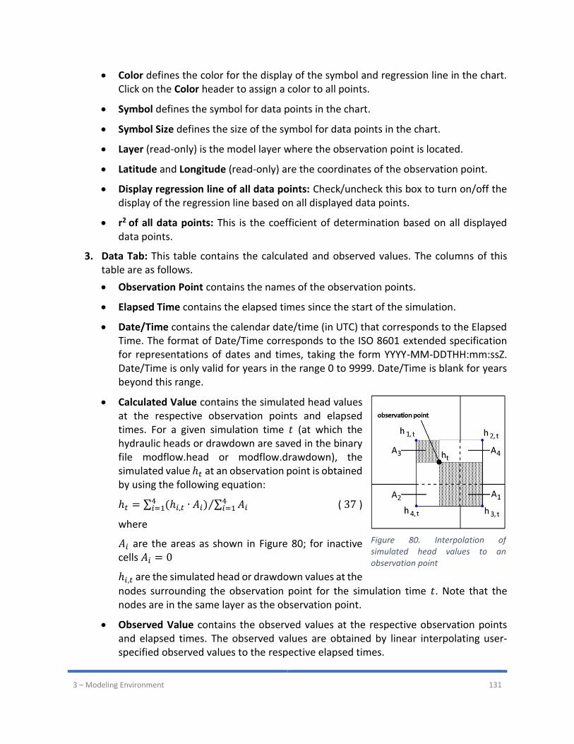
3 – Modeling Environment 131
• Color defines the color for the display of the symbol and regression line in the chart. Click on the Color header to assign a color to all points.
• Symbol defines the symbol for data points in the chart.
• Symbol Size defines the size of the symbol for data points in the chart.
• Layer (read-only) is the model layer where the observation point is located.
• Latitude and Longitude (read-only) are the coordinates of the observation point.
• Display regression line of all data points: Check/uncheck this box to turn on/off the display of the regression line based on all displayed data points.
• r2 of all data points: This is the coefficient of determination based on all displayed data points.
3. Data Tab: This table contains the calculated and observed values. The columns of this table are as follows.
• Observation Point contains the names of the observation points.
• Elapsed Time contains the elapsed times since the start of the simulation.
• Date/Time contains the calendar date/time (in UTC) that corresponds to the Elapsed Time. The format of Date/Time corresponds to the ISO 8601 extended specification for representations of dates and times, taking the form YYYY-MM-DDTHH:mm:ssZ. Date/Time is only valid for years in the range 0 to 9999. Date/Time is blank for years beyond this range.
• Calculated Value contains the simulated head values at the respective observation points and elapsed times. For a given simulation time 𝑡 (at which the hydraulic heads or drawdown are saved in the binary file modflow.head or modflow.drawdown), the simulated value ℎ𝑡 at an observation point is obtained by using the following equation:
ℎ𝑡 = ∑ (ℎ𝑖,𝑡 ∙ 𝐴𝑖)4𝑖=1 ∑ 𝐴𝑖
4𝑖=1⁄ ( 37 )
where
𝐴𝑖 are the areas as shown in Figure 80; for inactive cells 𝐴𝑖 = 0
ℎ𝑖,𝑡 are the simulated head or drawdown values at the
nodes surrounding the observation point for the simulation time 𝑡. Note that the nodes are in the same layer as the observation point.
• Observed Value contains the observed values at the respective observation points and elapsed times. The observed values are obtained by linear interpolating user-specified observed values to the respective elapsed times.
Figure 80. Interpolation of simulated head values to an observation point

3 – Modeling Environment 132
4. More Actions
• Activate: Switch on the selected observation points28.
• Deactivate: Switch off the selected observation points28.
• Save Chart: Select this item to display the Save Image dialog box that allows you to save the chart as in a support image format (JPEG, PNG, or BMP) or in the PDF format.
• Save Data: Select this item to display the Save Data dialog box that allows you to save the content of the Data table in a CSV file.
• Print Chart: Select this item to open the Print dialog box that enables you to print the chart.
Line Chart
To display the line chart based on the head data, select Line Chart > Head. To display the line
chart based on the drawdown data, select Line Chart > Drawdown. The Line Chart dialog box is
shown in Figure 81.
1. Chart: The chart displays a line graph using the simulated and observed data (see Data tab below). The x-axis represents the elapsed time since the start of the simulation and the y-axis represents the calculated and observed data. Two time-series curves are displayed for each observation point. Calculated and observed data points are represented by graphic symbols. Solid lines connect the calculated data and dashed lines connect the observed data. To interact with the chart, follow these steps:
• When the mouse cursor is moved into the chart, it becomes a crosshair (+), and the head (or drawdown) value, elapsed time, and corresponding calendar date/time are displayed next to the cursor.
• To pan around the chart, move the mouse cursor into the chart, press and hold the left mouse button, and then move the mouse.
• To zoom in/out on any part of the chart, place the mouse cursor within the chart, scroll the mouse wheel forward or backward.
• You can limit the zoom and pan to the x or y direction by selecting the x or y-axis first. An axis is selected by clicking on it. A selected axis is colored in blue. To deselect an axis, simply click on any part of the respective chart.
• To highlight the time-series curves of an observation point, click on a curve or a data point symbol. The corresponding row in the Observation Points table will be highlighted. Alternatively, you can highlight the time-series curves of an observation point by clicking on the respective Name field in the Observation Points table.
28 You may select multiple rows from the Observation Point table by using combinations of Ctrl-click and Shift-click.
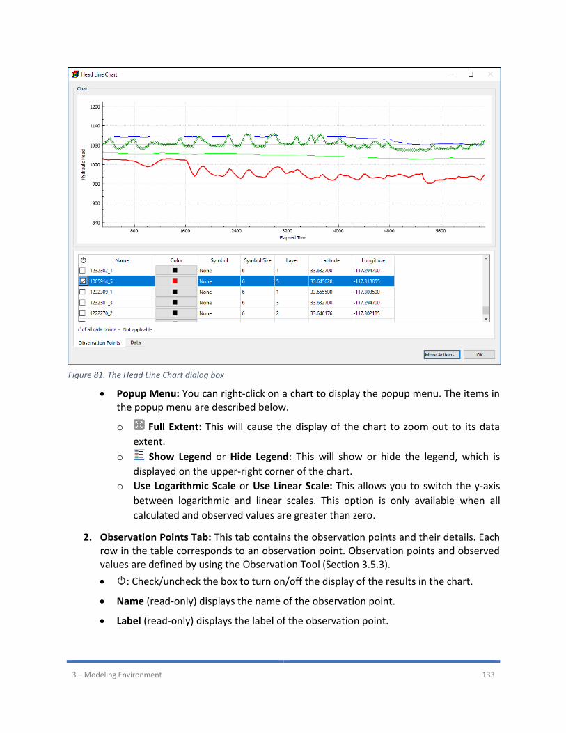
3 – Modeling Environment 133
• Popup Menu: You can right-click on a chart to display the popup menu. The items in the popup menu are described below.
o Full Extent: This will cause the display of the chart to zoom out to its data
extent.
o Show Legend or Hide Legend: This will show or hide the legend, which is
displayed on the upper-right corner of the chart.
o Use Logarithmic Scale or Use Linear Scale: This allows you to switch the y-axis
between logarithmic and linear scales. This option is only available when all
calculated and observed values are greater than zero.
2. Observation Points Tab: This tab contains the observation points and their details. Each row in the table corresponds to an observation point. Observation points and observed values are defined by using the Observation Tool (Section 3.5.3).
• : Check/uncheck the box to turn on/off the display of the results in the chart.
• Name (read-only) displays the name of the observation point.
• Label (read-only) displays the label of the observation point.
Figure 81. The Head Line Chart dialog box
3 – Modeling Environment 134
• Color defines the color for the display of the symbol and time-series curves in the chart.
• Symbol defines the symbol for data points in the chart.
• Symbol Size defines the size of the symbol for data points in the chart.
• Layer (read-only) is the model layer where the observation point is located.
• Latitude and Longitude (read-only) are the coordinates of the observation point.
• r2 of all data points: This is the coefficient of determination based on all calculated and observed data pairs of observation points that are turned on. Note that 𝑟2 always equals to 1 if there are only two data points.
3. Data Tab: This table contains the calculated and observed values. The contents of this table are the same as those of the Scatter Chart dialog box. See the previous section for details.
4. More Actions: The functionalities of this menu are the same as those of the Scatter Chart dialog box. See the previous section for details.
Volume Summary
Select this menu item to calculate the amount of water in the model based on the starting
hydraulic head, the simulated hydraulic head (stored in the modflow.head file), layer types
(unconfined, confined, or convertible), layer geometry (top and bottom elevation of layers), and
aquifer parameters (S, Ss, and Sy). If aquifer parameters are not specified, the respective default
values are used for the calculation.
The calculated results are stored in a comma-separated value file consisting of a number of
records. Each record represents storage terms in each time step and layer. A record includes the
following terms.
• ElapsedTime is the elapsed time (in the model time unit) since the start of the flow simulation.
• Period is the stress period. The records with Period = 0 represent the initial condition based on the starting hydraulic head.
• TimeStep is the time step within the given Period.
• Date is the calendar date in the form of year-month-day. The date corresponds to the given Period and TimeStep.
• Layer is the model layer.
• Vs [L3] is the volume of water stored due to compressibility (based on S or Ss) of the given date and layer. The volume of water stored in a cell due to compressibility (𝑣𝑠) is calculated based on the following rules.
o For confined/convertible layers:
3 – Modeling Environment 135
𝑣𝑠 = (𝑡 − 𝑏) × 𝐴𝑟𝑒𝑎 × 𝑆𝑠 × (ℎ − 𝑧) 𝑖𝑓 ℎ ≥ 𝑡
𝑣𝑠 = (ℎ − 𝑏) × 𝐴𝑟𝑒𝑎 × 𝑆𝑠 × ((ℎ − 𝑏)/2) 𝑖𝑓 𝑏 < ℎ < 𝑡
𝑣𝑠 = 0 𝑖𝑓 ℎ ≤ 𝑏
Where
𝑆𝑠 [L-1] is the specific storage of the cell,
ℎ [L] is the hydraulic head in the cell,
𝑧 [L] is the elevation of the center of the cell,
𝑡 [L] is the elevation of the top of the cell, and
𝑏 [L] is the elevation of the bottom of the cell, and
𝐴𝑟𝑒𝑎 [L2] is the area of the cell,
(ℎ − 𝑏) is the saturated thickness of the cell when it is not under confined condition, and
(ℎ − 𝑏) 2⁄ represents the average hydraulic head that acts on the water within the cell when it is not under confined condition.
o For unconfined layers:
𝑣𝑠 = (ℎ − 𝑏) × 𝐴𝑟𝑒𝑎 × 𝑆𝑠 × ((ℎ − 𝑏) 2⁄ ) 𝑖𝑓 ℎ > 𝑏
𝑣𝑠 = 0 𝑖𝑓 ℎ ≤ 𝑏
• Vsy [L3] is the amount of water stored in the pore space (based on Sy) of the given date and layer. The amount of water stored in the pore space of a cell (𝑣𝑠𝑦) is calculated based on the following rules.
o For confined/convertible layers:
𝑣𝑠𝑦 = (𝑡 − 𝑏) × 𝐴𝑟𝑒𝑎 × 𝑆𝑦 𝑖𝑓 ℎ ≥ 𝑡
𝑣𝑠𝑦 = (ℎ − 𝑏) × 𝐴𝑟𝑒𝑎 × 𝑆𝑦 𝑖𝑓 𝑏 < ℎ < 𝑡
𝑣𝑠𝑦 = 0 𝑖𝑓 ℎ ≤ 𝑏
Where
𝑆𝑦 [-] is the specific yield of the cell.
o For unconfined layers:
𝑣𝑠𝑦 = (ℎ − 𝑏) × 𝐴𝑟𝑒𝑎 × 𝑆𝑦 𝑖𝑓 ℎ > 𝑏
𝑣𝑠𝑦 = 0 𝑖𝑓 ℎ ≤ 𝑏
• Volume [L3] is the total amount of water of the model at the given date. The value is only calculated for the record with Layer equals to the bottom layer of the model.

3 – Modeling Environment 136
3.8.2. ZoneBudget
There are situations in which it is useful to calculate flow terms for various subregions of the
modeled area. To facilitate such calculations, MODFLOW saves the computed flow terms for
individual cells in the cell-by-cell budget file (i.e., the modflow.flow file within PM). Zonebudget
(Harbaugh, 1990) is a program that reads the budget file and produces water budgets for
subregions of the modeled area.
The individual cell flows are referred to as cell-by-cell flow terms, including (1) inflows or outflows
due to external stresses or boundaries, such as pumping well, recharge, or general-head
boundary; (2) storage changes; (3) flows from or to constant-head boundary; and (4) flows across
cell faces. ZoneBudget calculates the flow between adjacent zones based on the flow across cell
faces.
Follow the steps below to compute water budgets with ZoneBudget.
1. Define Zone Numbers with the Data Editor by selecting Models > ZoneBudget > Zones.
• If zone numbers are not defined, the entire model will be treated as a single zone, with the zone number set to 1.
• Zone numbers from 0 to 999 are allowed. The number 0 indicates that a cell is not associated with any zone and will be excluded from the zone budget calculation.
2. Run the ZoneBudget program by selecting Models > ZoneBudget > Run.
• PM will build the input file to the ZoneBudget and then start the ZoneBudget program.
• The run progress of ZoneBudget will be displayed in the ZoneBudget Output window. You may terminate the simulation at any time by clicking on the Terminate button. Once the calculation is complete, you can click the Close button to close the window.
3. Review the results:
• Models > ZoneBudget > View > Listing File: This listing file contains the water budget of all zones of individual time steps at which flow terms are saved in the budget file.
• Models > ZoneBudget > View > CSV File: For each time, for which the flow terms are saved in the budget file, there is one line for each in-flow term and each out-flow term along with totals. The zones are displayed in columns, so one table displays all zones. This makes it easy to compare any budget term for all the different zones. The CSV file is formatted in the way suitable to be loaded into a spreadsheet application.
• Models > ZoneBudget > View > CSV2 File29: The CSV2 file displays the complete budget for one zone and one time in a single line. Each column has a separate inflow or outflow budget term. The rows can be sorted by time within the spreadsheet
29 At the time of writing, if a package (such as general-head boundary) is active in the flow model, but no cells are defined for that package in a stress period, the inflow and outflow budget term of that package will be excluded for that stress period, leading to an incorrectly formatted CSV2 file.
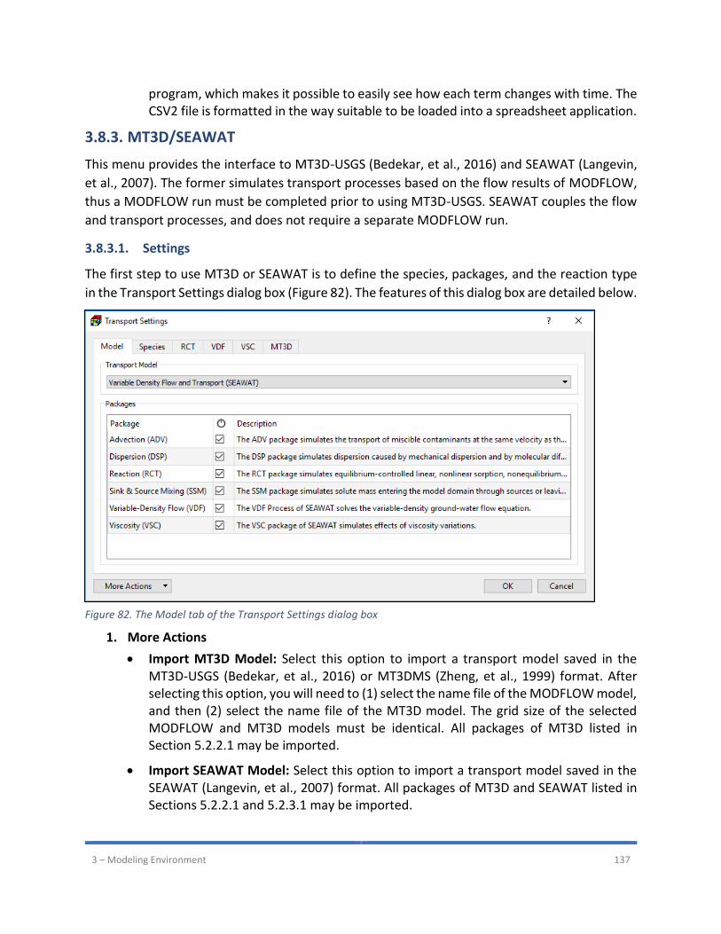
3 – Modeling Environment 137
program, which makes it possible to easily see how each term changes with time. The CSV2 file is formatted in the way suitable to be loaded into a spreadsheet application.
3.8.3. MT3D/SEAWAT
This menu provides the interface to MT3D-USGS (Bedekar, et al., 2016) and SEAWAT (Langevin,
et al., 2007). The former simulates transport processes based on the flow results of MODFLOW,
thus a MODFLOW run must be completed prior to using MT3D-USGS. SEAWAT couples the flow
and transport processes, and does not require a separate MODFLOW run.
3.8.3.1. Settings
The first step to use MT3D or SEAWAT is to define the species, packages, and the reaction type
in the Transport Settings dialog box (Figure 82). The features of this dialog box are detailed below.
1. More Actions
• Import MT3D Model: Select this option to import a transport model saved in the MT3D-USGS (Bedekar, et al., 2016) or MT3DMS (Zheng, et al., 1999) format. After selecting this option, you will need to (1) select the name file of the MODFLOW model, and then (2) select the name file of the MT3D model. The grid size of the selected MODFLOW and MT3D models must be identical. All packages of MT3D listed in Section 5.2.2.1 may be imported.
• Import SEAWAT Model: Select this option to import a transport model saved in the SEAWAT (Langevin, et al., 2007) format. All packages of MT3D and SEAWAT listed in Sections 5.2.2.1 and 5.2.3.1 may be imported.
Figure 82. The Model tab of the Transport Settings dialog box
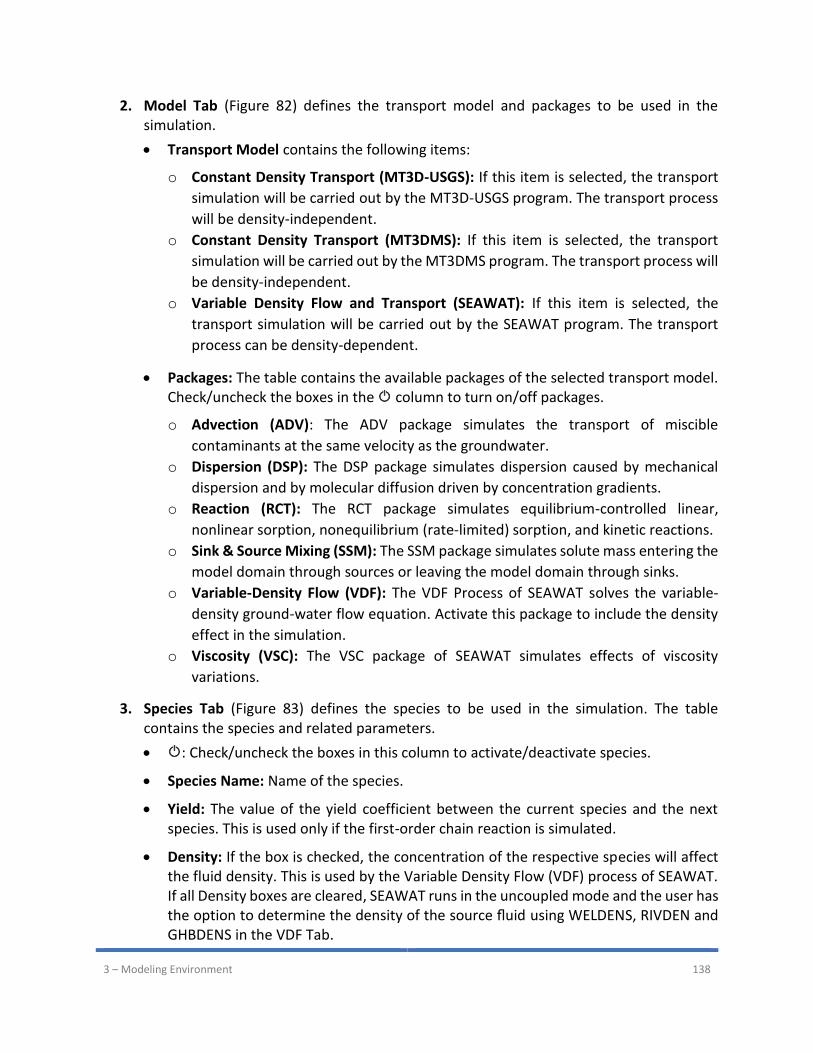
3 – Modeling Environment 138
2. Model Tab (Figure 82) defines the transport model and packages to be used in the simulation.
• Transport Model contains the following items:
o Constant Density Transport (MT3D-USGS): If this item is selected, the transport
simulation will be carried out by the MT3D-USGS program. The transport process
will be density-independent.
o Constant Density Transport (MT3DMS): If this item is selected, the transport
simulation will be carried out by the MT3DMS program. The transport process will
be density-independent.
o Variable Density Flow and Transport (SEAWAT): If this item is selected, the
transport simulation will be carried out by the SEAWAT program. The transport
process can be density-dependent.
• Packages: The table contains the available packages of the selected transport model. Check/uncheck the boxes in the column to turn on/off packages.
o Advection (ADV): The ADV package simulates the transport of miscible
contaminants at the same velocity as the groundwater.
o Dispersion (DSP): The DSP package simulates dispersion caused by mechanical
dispersion and by molecular diffusion driven by concentration gradients.
o Reaction (RCT): The RCT package simulates equilibrium-controlled linear,
nonlinear sorption, nonequilibrium (rate-limited) sorption, and kinetic reactions.
o Sink & Source Mixing (SSM): The SSM package simulates solute mass entering the
model domain through sources or leaving the model domain through sinks.
o Variable-Density Flow (VDF): The VDF Process of SEAWAT solves the variable-
density ground-water flow equation. Activate this package to include the density
effect in the simulation.
o Viscosity (VSC): The VSC package of SEAWAT simulates effects of viscosity
variations.
3. Species Tab (Figure 83) defines the species to be used in the simulation. The table contains the species and related parameters.
• : Check/uncheck the boxes in this column to activate/deactivate species.
• Species Name: Name of the species.
• Yield: The value of the yield coefficient between the current species and the next species. This is used only if the first-order chain reaction is simulated.
• Density: If the box is checked, the concentration of the respective species will affect the fluid density. This is used by the Variable Density Flow (VDF) process of SEAWAT. If all Density boxes are cleared, SEAWAT runs in the uncoupled mode and the user has the option to determine the density of the source fluid using WELDENS, RIVDEN and GHBDENS in the VDF Tab.
3 – Modeling Environment 139
• DRHODC is the slope that relates fluid density (ρ) to solute concentration (C), i.e., ∂ρ/∂C. This is used by the Variable Density Flow (VDF) process of SEAWAT.
• CRHOREF is the reference concentration (i.e., C0) for the species. For most simulations, CRHOREF should be specified as zero. This is used by the Variable Density Flow (VDF) process of SEAWAT.
• Viscosity: If the box is checked, the effects of viscosity variations are activated for the corresponding species. This is used by the Viscosity (VSC) package of SEAWAT.
• DMUDC is the slope that relates dynamic viscosity (μ) to solute concentration (C), i.e., ∂μ/∂C. This is used by the Viscosity (VSC) package of SEAWAT.
• CMUREF is the reference concentration for the species. This is used by the Viscosity (VSC) package of SEAWAT.
4. RCT Tab (Figure 84) contains options for the Reaction Package. The available sorption and reaction types and their required parameters are described as follows. The required parameters for the selected options must be specified in the Models > MT3D/SEAWAT > Packages > Reaction (RCT) menu.
• Sorption:
o Sorption Type defines the type of sorption or dual-domain transfer. Equilibrium-
controlled sorption isotherms are implemented in MT3D through use of the
retardation factor R.
No sorption: Sorption is not simulated.
Figure 83. The Species Tab of the Transport Settings dialog box
3 – Modeling Environment 140
Linear Isotherm simulates linear equilibrium sorption and assumes that the
sorbed concentration 𝐶 is directly proportional to the dissolved concentration
𝐶. The retardation factor 𝑅 is therefore independent of the concentration
values and is calculated only once for each cell at the beginning of the
simulation.
𝐶̅ = 𝐾𝑑 ⋅ 𝐶 ( 38 )
𝑅 = 1 + 𝜌𝑏
𝑛⋅ 𝐾𝑑 ( 39 )
where n [-] is the porosity of the porous medium in a cell; 𝐾𝑑 [L3M-1] is the
distribution coefficient that depends on the solute species, nature of the
porous medium, and other conditions of the system; and 𝜌𝑏 [ML-3] is the bulk
density of the porous medium of the cell.
Freundlich Isotherm simulates nonlinear equilibrium sorption with the
following equation.
𝐶 = 𝐾𝑓 ⋅ 𝐶𝑎 ( 40 )
The retardation factor at the beginning of a transport step is calculated by
𝑅 = 1 + 𝜌𝑏
𝑛⋅ 𝑎 ⋅ 𝐶𝑎−1 ⋅ 𝐾𝑓 ( 41 )
Where 𝐶 is the solute concentration in a cell at the beginning of a transport
step; 𝑎 [-] is the Freundlich exponent; and 𝐾𝑓 [L3M-1] is the Freundlich constant.

3 – Modeling Environment 141
Langmuir Isotherm simulates nonlinear equilibrium sorption with the following
equation.
𝐶 = (𝐾𝐿 ⋅ 𝑆 ⋅ 𝐶) (1 + 𝐾𝐿 ⋅ 𝐶 )⁄ ( 42 )
The retardation factor at the beginning of a transport step is calculated by
𝑅 = 1 + 𝜌𝑏
𝑛⋅
𝐾𝐿⋅𝑆
(1+𝐾𝐿⋅𝐶 )2 ( 43 )
where 𝐾𝐿 [L3M-1] is the Langmuir constant and 𝑆 [MM-1] is the sorption capacity
of the porous medium.
First-order Kinetic Sorption simulates nonequilibrium sorption. It is assumed
that sorption can be represented by a first-order reversible kinetic sorption
defined by
𝜌𝑏 ⋅𝜕𝐶
𝜕𝑡= 𝛽 ⋅ (𝐶 −
𝐶
𝐾𝑑) ( 44 )
Where 𝛽 [T-1] is the first-order mass transfer rate between the dissolved and sorbed phases.
Dual-Domain Mass Transfer (without Sorption), Dual-Domain Mass Transfer
(with Sorption), and Dual-Domain Mass Transfer (with Different Sorption
Coefficients in Mobile and Immobile Domains): Dual-domain means that two
kinds of continuum, e.g. a fractured medium and the porous medium, exist
simultaneously in the same spatial region, i.e., the same model cells. In
Figure 84. The RCT tab of the Transport Settings dialog box
3 – Modeling Environment 142
fractured aquifers, water moves faster along fractures than it does in a rock
formation and the solute transport is often controlled by advection along the
fractures and dominated by dispersion in the porous block along the fractures.
MT3D uses the dual-domain concept to approach extremely heterogeneous
porous media or media composed of fractures and pores. In this approach, the
effective porosity is used as the primary porosity for the pore spaces filled with
mobile water (i.e., fractures) and the secondary porosity for the pore spaces
filled with immobile water (i.e., rock formation) is defined separately. The sum
of the primary and the secondary porosities is the total porosity of the medium.
The sorption process in the mobile and immobile domain is simulated by using
the linear isotherm.
The exchange of the dissolved mass between the mobile and immobile domains
can be defined by
𝑛𝑖𝑚 ⋅𝜕𝐶𝑖𝑚
𝜕𝑡= 𝜁 ⋅ (𝐶𝑚 − 𝐶𝑖𝑚) ( 45 )
where 𝑛𝑖𝑚 [-] is the porosity of the immobile domain; 𝐶𝑖𝑚 [ML-3] is the solute
concentration in the immobile domain; 𝐶𝑚 [ML-3] is the solute concentration in
the mobile domain; and 𝜁 [T-1] is the first-order mass transfer rate between
the mobile and immobile domains. As the mass transfer rate 𝜁 increases, the
dual-domain model functions more and more like the single-domain model
with a porosity approaching the total porosity of the porous medium.
o IGETSC is a flag indicating whether the initial concentration for the non-
equilibrium sorbed or immobile phase of all species should be read when first-
order kinetic sorption or dual-domain mass transfer is simulated.
If this box is checked, the initial concentration for the sorbed phase or immobile
liquid phase of all species will be used in the simulation.
If this box is unchecked, the initial concentration for the sorbed or immobile
phase is not used. The sorbed phase is assumed to be in equilibrium with the
dissolved phase and the immobile domain is assumed to have zero
concentration.
• Kinetic Rate Reaction defines the type of kinetic rate reaction. Note that first-order irreversible reaction and MONOD kinetic reaction are not intended for modeling chemical reactions between species.
o No Kinetic Rate Reaction: kinetic rate reaction is not simulated.
o Zero-order Reaction: The reaction rate of a zero-order reaction is constant and
independent of the concentration of reacting substances. In MT3D, the zero-order

3 – Modeling Environment 143
reaction rate coefficients for the dissolved phase (in [ML-3T-1]) and sorbed phase
(in [MM-1T-1]) may be specified separately. The convention for both coefficients
are positive values for decay and negative values for production.
o First-order Irreversible Reaction: The concentration change due to the chemical
reaction from one transport step to another at a cell can be expressed as
Δ𝐶 = −Δ𝑡
𝑅⋅ [𝜆1 ⋅ 𝐶 + 𝜆2 ⋅
𝜌𝑏
𝑛⋅ 𝐶̅] ( 46 )
where 𝜆1 [T-1] is the first-order rate for the dissolved phase; 𝜆2 [T-1] is the first-order rate for the sorbed phase; Δ𝑡 is the transport time-step; and 𝐶̅ is the mass of the solute species adsorbed on the solids per unit bulk dry mass of the porous medium at the beginning of each transport step. 𝐶̅ is in equilibrium with solute concentration 𝐶 in the cell.
The rate constant 𝜆 is usually given in terms of the half-life. Generally, if the reaction is radioactive decay, 𝜆2 should be set equal to 𝜆1. However, for certain types of biodegradation, 𝜆2 may be different.
o First-order Chain Reaction: The first-order chain reaction is implemented in MT3D
for both dissolved and sorbed phases. Considering the dissolved phase, the
changes in the concentration values of involved species within a transport time-
step are calculated in the following sequential order:
𝛥𝐶1
𝛥𝑡= −𝜆1 ⋅ 𝐶1
𝛥𝐶2
𝛥𝑡= −𝜆2 ⋅ 𝐶2 + 𝑌1 2⁄ ⋅ 𝜆1 ⋅ 𝐶1 ( 47 )
… 𝛥𝐶𝑘
𝛥𝑡= −𝜆𝑘 ⋅ 𝐶𝑘 + 𝑌𝑘−1 k⁄ ⋅ 𝜆𝑘−1 ⋅ 𝐶𝑘−1
where 𝜆𝑘 specifies the first-order reaction coefficient for species k and 𝑌𝑘−1 k⁄ sets
the yield coefficient between species k-1 and k. Yield coefficients are based on stoichiometric relations between the species for which relations are specified.
o Monod Kinetic Reaction: The concentration change due to the chemical reaction
from one transport step to another at a cell can be expressed by
𝛥𝐶 = −𝑀𝑖𝑐𝑡 ⋅ 𝜇𝑚𝑎𝑥 ⋅𝐶
𝐾𝑠+𝐶 ( 48 )
where
𝑀𝑖𝑐𝑡 is the total microbial concentration [ML-3] at the cell,
𝐾𝑠 is a constant, described by (Alexander, 1999), called the half-saturation constant, and is equal to the constituent concentration [ML-3] at which the microbial growth rate is half of 𝜇𝑚𝑎𝑥. It is important to note that the microbial concentration depends on many chemical and biological considerations and is
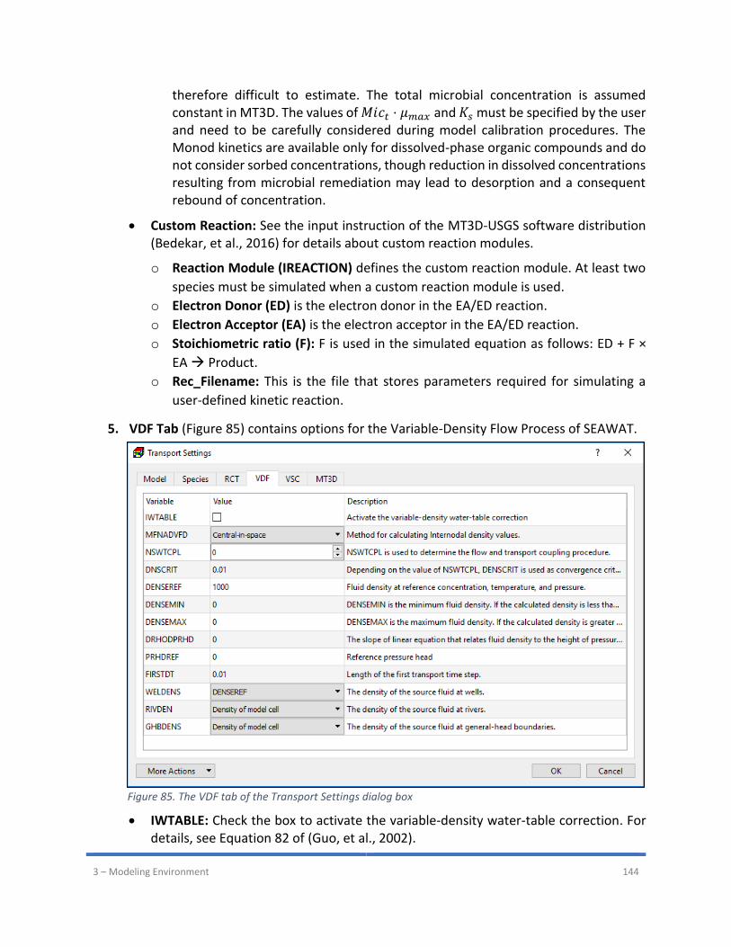
3 – Modeling Environment 144
therefore difficult to estimate. The total microbial concentration is assumed constant in MT3D. The values of 𝑀𝑖𝑐𝑡 ⋅ 𝜇𝑚𝑎𝑥 and 𝐾𝑠 must be specified by the user and need to be carefully considered during model calibration procedures. The Monod kinetics are available only for dissolved-phase organic compounds and do not consider sorbed concentrations, though reduction in dissolved concentrations resulting from microbial remediation may lead to desorption and a consequent rebound of concentration.
• Custom Reaction: See the input instruction of the MT3D-USGS software distribution (Bedekar, et al., 2016) for details about custom reaction modules.
o Reaction Module (IREACTION) defines the custom reaction module. At least two
species must be simulated when a custom reaction module is used.
o Electron Donor (ED) is the electron donor in the EA/ED reaction.
o Electron Acceptor (EA) is the electron acceptor in the EA/ED reaction.
o Stoichiometric ratio (F): F is used in the simulated equation as follows: ED + F ×
EA Product.
o Rec_Filename: This is the file that stores parameters required for simulating a
user-defined kinetic reaction.
5. VDF Tab (Figure 85) contains options for the Variable-Density Flow Process of SEAWAT.
• IWTABLE: Check the box to activate the variable-density water-table correction. For details, see Equation 82 of (Guo, et al., 2002).
Figure 85. The VDF tab of the Transport Settings dialog box
3 – Modeling Environment 145
• MFNADVFD this defines the method for calculating Internodal density values.
• NSWTCPL is used to determine the flow and transport coupling procedure.
o If NSWTCPL = 0 or 1, flow and transport will be explicitly coupled using a one-
timestep lag. The explicit coupling option is normally much faster than the
iterative option and is recommended for most applications.
o If NSWTCPL > 1, NSWTCPL is the maximum number of non-linear coupling
iterations for the flow and transport solutions. SEAWAT-2000 will stop execution
after NSWTCPL iterations if convergence between flow and transport has not
occurred.
o If NSWTCPL = -1, the flow solution will be recalculated only for
The first transport step of the simulation, or
The last transport step of the MODFLOW time step, or
The maximum density change at a cell is greater than DNSCRIT.
• DNSCRIT: Depending on the value of NSWTCPL, DENSCRIT is used as convergence criterion or maximum density threshold.
o If NSWTCPL > 1, DNSCRIT is the convergence criterion for convergence between
flow and transport. If the maximum fluid density difference between two
consecutive implicit coupling iterations is not less than DNSCRIT, the program will
continue to iterate on the flow and transport equations, or will terminate if
NSWTCPL is reached.
o If NSWTCPL is -1, DNSCRIT is the maximum density threshold. If the fluid density
change (between the present transport time step and the last flow solution) at
one or more cells is greater than DNSCRIT, then SEAWAT will update the flow field
(by solving the flow equation with the updated density field).
• DENSEREF is the fluid density at reference concentration, temperature, and pressure.
• DENSEMIN is the minimum fluid density. If the calculated density is less than DENSEMIN, it is set to DENSEMIN. To remove this limitation, set DENSEMIN to zero.
• DENSEMAX is the maximum fluid density. If the calculated density is greater than DENSEMAX, it is set to DENSEMAX. To remove the limitation, set DENSEMAX to zero.
• DRHODPRHD is the slope of linear equation that relates fluid density to the height of pressure head.
• PRHDREF is the reference pressure head.
• FIRSTDT is the length of the first transport time step.
• DRNBELEV
3 – Modeling Environment 146
o User-specified in the DRN Package: the user-specified values of Elevation of Drain
Bottom will be assigned to the auxiliary variable DRNBELEV in the input file to the
DRN package and used for the Variable-Density Flow (VDF) process of a SEAWAT
simulation.
o Elevation of model cell center: the auxiliary variable DRNBELEV will not be
assigned to the input file to the DRN package, consequently the cell center
elevation will be used by the VDF process of SEAWAT.
• DRTBELEV
o User-specified in the DRT Package: the user-specified values of Elevation of Drain
Bottom will be assigned to the auxiliary variable DRTBELEV in the input file to the
DRT package and used for the Variable-Density Flow (VDF) process of a SEAWAT
simulation.
o Elevation of model cell center: the auxiliary variable DRTBELEV will not be
assigned to the input file to the DRT package, consequently the cell center
elevation will be used by the VDF process of SEAWAT.
• GHBDENS30 controls the density of the source fluid at general-head boundaries.
o User-specified in the GHB Package: the user-specified values of Water Density will
be assigned to the auxiliary variable GHBDENS in the input file to the GHB package
and used for the Variable-Density Flow (VDF) process of a SEAWAT simulation.
o Density of model cell: the auxiliary variable GHBDENS will not be assigned to the
input file to the GHB package and the calculated density of model cells will be used
by the VDF process of SEAWAT by default.
• GHBELEV:
o User-specified in the GHB Package: the user-specified values of GHB Elevation will
be assigned to the auxiliary variable GHBELEV in the input file to the GHB package
and used for the Variable-Density Flow (VDF) process of a SEAWAT simulation.
o Elevation of model cell center: the auxiliary variable GHBELEV will not be assigned
to the input file to the GHB package and the cell center elevation will be used by
the VDF process of SEAWAT by default.
• RIVDEN30 controls the density of the source fluid at rivers.
o User-specified in the RIV Package: the user-specified values of Water Density will
be assigned to the auxiliary variable RIVDEN in the input file to the RIV package
and used for the Variable-Density Flow (VDF) process of a SEAWAT simulation.
30 When all Density boxes in the Species tab are cleared (i.e., SEAWAT runs in the uncoupled mode), the user has the option to determine the density of the source fluid. The setting is ignored if the Density box of any of the species is checked.
3 – Modeling Environment 147
o Density of model cell: the auxiliary variable RIVDEN will not be assigned to the
input file to the RIV package and the calculated density of model cells will be used
by the VDF process of SEAWAT by default.
• RDBTHK
o User-specified in the RIV Package: the user-specified values of Thickness of
Riverbed Sediments will be assigned to the auxiliary variable RDBTHK in the input
file to the RIV package and used for the Variable-Density Flow (VDF) process of a
SEAWAT simulation.
o Difference between river bottom elevation and cell center: the auxiliary variable
RDBTHK will not be assigned to the input file to the RIV package and the difference
between the river bottom elevation and cell center elevation will be used by the
VDF process of SEAWAT.
• WELDENS30 controls the density of the source fluid at wells.
o User-specified in the WEL Package: the user-specified values of Water Density will
be assigned to the auxiliary variable WELDENS in the input file to the WEL package
and used for the Variable-Density Flow (VDF) process of a SEAWAT simulation.
o DENSEREF: the auxiliary variable WELDENS will not be assigned to the input file to
the WEL package and the value of DENSEREF will be used by the VDF process of
SEAWAT by default.
6. VSC Tab (Figure 86) contains Options for the Viscosity Package of SEAWAT.
• VISCMIN is the minimum fluid viscosity. If the calculated viscosity is less than VISCMIN, it is set to VISCMIN. To remove this limitation, set VISCMIN to zero.
• VISCMAX is the maximum fluid viscosity. If the calculated viscosity is greater than VISCMAX, it is set to VISCMAX. To remove the limitation, set VISCMAX to zero.
• VISCREF is the fluid viscosity at the reference concentration and reference temperature. For most simulations, VISCREF is specified as the viscosity of freshwater.
• MUTEMPOPT is the option for including the effect of temperature on fluid viscosity.
o MUTEMPOPT = 0, the effect of temperature on fluid viscosity is defined by
DMUDC and CMUREF of the species with the Viscosity box checked.
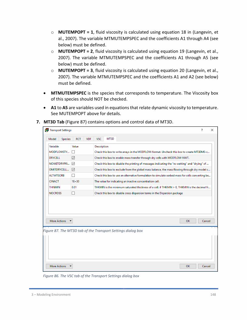
3 – Modeling Environment 148
o MUTEMPOPT = 1, fluid viscosity is calculated using equation 18 in (Langevin, et
al., 2007). The variable MTMUTEMPSPEC and the coefficients A1 through A4 (see
below) must be defined.
o MUTEMPOPT = 2, fluid viscosity is calculated using equation 19 (Langevin, et al.,
2007). The variable MTMUTEMPSPEC and the coefficients A1 through A5 (see
below) must be defined.
o MUTEMPOPT = 3, fluid viscosity is calculated using equation 20 (Langevin, et al.,
2007). The variable MTMUTEMPSPEC and the coefficients A1 and A2 (see below)
must be defined.
• MTMUTEMPSPEC is the species that corresponds to temperature. The Viscosity box of this species should NOT be checked.
• A1 to A5 are variables used in equations that relate dynamic viscosity to temperature. See MUTEMPOPT above for details.
7. MT3D Tab (Figure 87) contains options and control data of MT3D.
Figure 86. The VSC tab of the Transport Settings dialog box
Figure 87. The MT3D tab of the Transport Settings dialog box
3 – Modeling Environment 149
• MODFLOWSTYLEARRAY: Check this box to write arrays in the MODFLOW-format. Uncheck this box to create MT3DMS-compatible input files.
• DRYCELL: Check this box to enable mass transfer through dry cells with MODFLOW-NWT.
• NOWETDRYPRINT: Check this box to disable the printing of messages indicating the "re-wetting" and "drying" of model cells to the model run listing file.
• OMITDRYCELLBUDGET: Check this box to exclude from the global mass balance, the mass flowing through dry model cells.
• ALTWTSORB: Check this box to use an alternative formulation to simulate sorbed mass for cells converting between wet and dry.
• CINACT is the value for indicating an inactive concentration cell.
• THKMIN is the minimum saturated thickness of a cell.
o if THKMIN > 0, THKMIN is the decimal fraction of the model layer thickness,
o if THKMIN< 0, absolute value of THKMIN is used.
• NOCROSS: Check this box to disable cross dispersion terms in the Dispersion package. For most simulations, you should retain the cross-dispersion terms because they typically improve accuracy. For complex problems resulting in negative concentrations, the NOCROSS option provides a way to determine the cause of the negative concentrations.
3.8.3.2. Initial Concentration
At the beginning of a transport simulation, MT3D and SEAWAT require the initial concentration
of each active species at each active concentration cell, i.e. ICBUND > 0.
3.8.3.3. Packages
Advection (ADV)
The following parameters are defined in the Advection (ADV) Package dialog box (Figure 88).
1. Settings
• Advection Solution Option (MIXELM):
o Third-order TVD Scheme (ULTIMATE) is based on the ULTIMATE algorithm
(Leonard, 1988), which is in turn derived from the earlier QUICKEST algorithm
(Leonard, 1979). With the ULTIMATE scheme, the solution is mass conservative,
without excessive numerical dispersion and artificial oscillation.
o Finite-Difference Method is implicit with the Generalized Conjugate Gradient
solver (GCG) package. Due to the problems of numerical dispersion and artificial
oscillation, the upstream finite difference method is only suitable for solving
transport problems not dominated by advection. When the Peclet number 𝑃𝑒
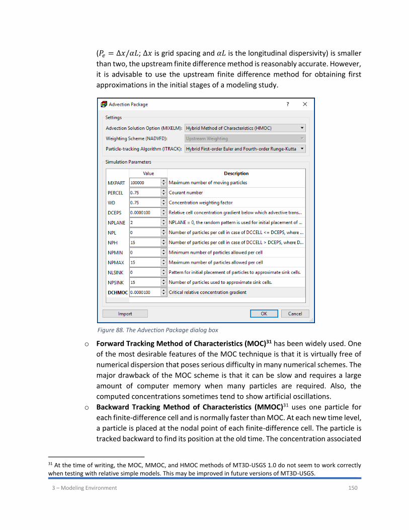
3 – Modeling Environment 150
(𝑃𝑒 = Δ𝑥/𝛼𝐿; Δ𝑥 is grid spacing and 𝛼𝐿 is the longitudinal dispersivity) is smaller
than two, the upstream finite difference method is reasonably accurate. However,
it is advisable to use the upstream finite difference method for obtaining first
approximations in the initial stages of a modeling study.
o Forward Tracking Method of Characteristics (MOC)31 has been widely used. One
of the most desirable features of the MOC technique is that it is virtually free of
numerical dispersion that poses serious difficulty in many numerical schemes. The
major drawback of the MOC scheme is that it can be slow and requires a large
amount of computer memory when many particles are required. Also, the
computed concentrations sometimes tend to show artificial oscillations.
o Backward Tracking Method of Characteristics (MMOC)31 uses one particle for
each finite-difference cell and is normally faster than MOC. At each new time level,
a particle is placed at the nodal point of each finite-difference cell. The particle is
tracked backward to find its position at the old time. The concentration associated
31 At the time of writing, the MOC, MMOC, and HMOC methods of MT3D-USGS 1.0 do not seem to work correctly when testing with relative simple models. This may be improved in future versions of MT3D-USGS.
Figure 88. The Advection Package dialog box
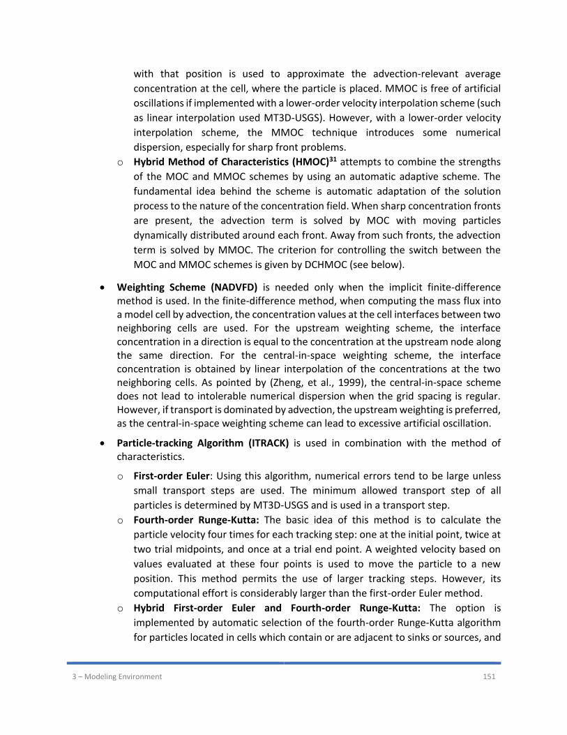
3 – Modeling Environment 151
with that position is used to approximate the advection-relevant average
concentration at the cell, where the particle is placed. MMOC is free of artificial
oscillations if implemented with a lower-order velocity interpolation scheme (such
as linear interpolation used MT3D-USGS). However, with a lower-order velocity
interpolation scheme, the MMOC technique introduces some numerical
dispersion, especially for sharp front problems.
o Hybrid Method of Characteristics (HMOC)31 attempts to combine the strengths
of the MOC and MMOC schemes by using an automatic adaptive scheme. The
fundamental idea behind the scheme is automatic adaptation of the solution
process to the nature of the concentration field. When sharp concentration fronts
are present, the advection term is solved by MOC with moving particles
dynamically distributed around each front. Away from such fronts, the advection
term is solved by MMOC. The criterion for controlling the switch between the
MOC and MMOC schemes is given by DCHMOC (see below).
• Weighting Scheme (NADVFD) is needed only when the implicit finite-difference method is used. In the finite-difference method, when computing the mass flux into a model cell by advection, the concentration values at the cell interfaces between two neighboring cells are used. For the upstream weighting scheme, the interface concentration in a direction is equal to the concentration at the upstream node along the same direction. For the central-in-space weighting scheme, the interface concentration is obtained by linear interpolation of the concentrations at the two neighboring cells. As pointed by (Zheng, et al., 1999), the central-in-space scheme does not lead to intolerable numerical dispersion when the grid spacing is regular. However, if transport is dominated by advection, the upstream weighting is preferred, as the central-in-space weighting scheme can lead to excessive artificial oscillation.
• Particle-tracking Algorithm (ITRACK) is used in combination with the method of characteristics.
o First-order Euler: Using this algorithm, numerical errors tend to be large unless
small transport steps are used. The minimum allowed transport step of all
particles is determined by MT3D-USGS and is used in a transport step.
o Fourth-order Runge-Kutta: The basic idea of this method is to calculate the
particle velocity four times for each tracking step: one at the initial point, twice at
two trial midpoints, and once at a trial end point. A weighted velocity based on
values evaluated at these four points is used to move the particle to a new
position. This method permits the use of larger tracking steps. However, its
computational effort is considerably larger than the first-order Euler method.
o Hybrid First-order Euler and Fourth-order Runge-Kutta: The option is
implemented by automatic selection of the fourth-order Runge-Kutta algorithm
for particles located in cells which contain or are adjacent to sinks or sources, and
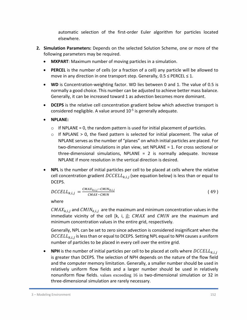
3 – Modeling Environment 152
automatic selection of the first-order Euler algorithm for particles located
elsewhere.
2. Simulation Parameters: Depends on the selected Solution Scheme, one or more of the following parameters may be required.
• MXPART: Maximum number of moving particles in a simulation.
• PERCEL is the number of cells (or a fraction of a cell) any particle will be allowed to move in any direction in one transport step. Generally, 0.5 ≤ PERCEL ≤ 1.
• WD is Concentration-weighting factor. WD lies between 0 and 1. The value of 0.5 is normally a good choice. This number can be adjusted to achieve better mass balance. Generally, it can be increased toward 1 as advection becomes more dominant.
• DCEPS is the relative cell concentration gradient below which advective transport is considered negligible. A value around 10-5 is generally adequate.
• NPLANE:
o If NPLANE = 0, the random pattern is used for initial placement of particles.
o If NPLANE > 0, the fixed pattern is selected for initial placement. The value of
NPLANE serves as the number of “planes” on which initial particles are placed. For
two-dimensional simulations in plan view, set NPLANE = 1. For cross sectional or
three-dimensional simulations, NPLANE = 2 is normally adequate. Increase
NPLANE if more resolution in the vertical direction is desired.
• NPL is the number of initial particles per cell to be placed at cells where the relative cell concentration gradient 𝐷𝐶𝐶𝐸𝐿𝐿𝑘,𝑖,𝑗 (see equation below) is less than or equal to
DCEPS.
𝐷𝐶𝐶𝐸𝐿𝐿𝑘,𝑖,𝑗 =𝐶𝑀𝐴𝑋𝑘,𝑖,𝑗−𝐶𝑀𝐼𝑁𝑘,𝑖,𝑗
𝐶𝑀𝐴𝑋−𝐶𝑀𝐼𝑁 ( 49 )
where
𝐶𝑀𝐴𝑋𝑘,𝑖,𝑗 and 𝐶𝑀𝐼𝑁𝑘,𝑖,𝑗 are the maximum and minimum concentration values in the
immediate vicinity of the cell [k, i, j]; 𝐶𝑀𝐴𝑋 and 𝐶𝑀𝐼𝑁 are the maximum and minimum concentration values in the entire grid, respectively.
Generally, NPL can be set to zero since advection is considered insignificant when the 𝐷𝐶𝐶𝐸𝐿𝐿𝑘,𝑖,𝑗 is less than or equal to DCEPS. Setting NPL equal to NPH causes a uniform
number of particles to be placed in every cell over the entire grid.
• NPH is the number of initial particles per cell to be placed at cells where 𝐷𝐶𝐶𝐸𝐿𝐿𝑘,𝑖,𝑗
is greater than DCEPS. The selection of NPH depends on the nature of the flow field and the computer memory limitation. Generally, a smaller number should be used in relatively uniform flow fields and a larger number should be used in relatively nonuniform flow fields. values exceeding 16 in two-dimensional simulation or 32 in three-dimensional simulation are rarely necessary.
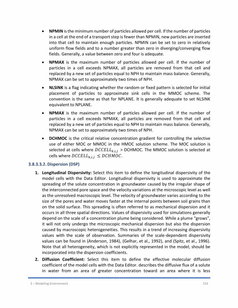
3 – Modeling Environment 153
• NPMIN is the minimum number of particles allowed per cell. If the number of particles in a cell at the end of a transport step is fewer than NPMIN, new particles are inserted into that cell to maintain enough particles. NPMIN can be set to zero in relatively uniform flow fields and to a number greater than zero in diverging/converging flow fields. Generally, a value between zero and four is adequate.
• NPMAX is the maximum number of particles allowed per cell. If the number of particles in a cell exceeds NPMAX, all particles are removed from that cell and replaced by a new set of particles equal to NPH to maintain mass balance. Generally, NPMAX can be set to approximately two times of NPH.
• NLSINK is a flag indicating whether the random or fixed pattern is selected for initial placement of particles to approximate sink cells in the MMOC scheme. The convention is the same as that for NPLANE. It is generally adequate to set NLSINK equivalent to NPLANE.
• NPMAX is the maximum number of particles allowed per cell. If the number of particles in a cell exceeds NPMAX, all particles are removed from that cell and replaced by a new set of particles equal to NPH to maintain mass balance. Generally, NPMAX can be set to approximately two times of NPH.
• DCHMOC is the critical relative concentration gradient for controlling the selective use of either MOC or MMOC in the HMOC solution scheme. The MOC solution is selected at cells where 𝐷𝐶𝐶𝐸𝐿𝐿𝑘,𝑖,𝑗 > DCHMOC. The MMOC solution is selected at
cells where 𝐷𝐶𝐶𝐸𝐿𝐿𝑘,𝑖,𝑗 ≤ 𝐷𝐶𝐻𝑀𝑂𝐶.
Dispersion (DSP)
1. Longitudinal Dispersivity: Select this item to define the longitudinal dispersivity of the model cells with the Data Editor. Longitudinal dispersivity is used to approximate the spreading of the solute concentration in groundwater caused by the irregular shape of the interconnected pore space and the velocity variations at the microscopic level as well as the unresolved macroscopic level. The velocity of groundwater varies according to the size of the pores and water moves faster at the internal points between soil grains than on the solid surface. This spreading is often referred to as mechanical dispersion and it occurs in all three spatial directions. Values of dispersivity used for simulations generally depend on the scale of a concentration plume being considered. While a plume “grows”, it will not only undergo the microscopic mechanical dispersion but also the dispersion caused by macroscopic heterogeneities. This results in a trend of increasing dispersivity values with the scale of observation. Summaries of the scale-dependent dispersivity values can be found in (Anderson, 1984), (Gelhar, et al., 1992), and (Spitz, et al., 1996). Note that all heterogeneity, which is not explicitly represented in the model, should be incorporated into the dispersion coefficients.
2. Diffusion Coefficient: Select this item to define the effective molecular diffusion coefficient of the model cells with the Data Editor. describes the diffusive flux of a solute in water from an area of greater concentration toward an area where it is less
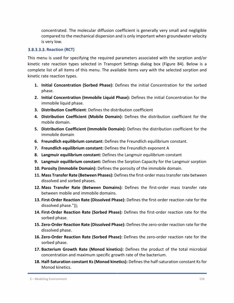
3 – Modeling Environment 154
concentrated. The molecular diffusion coefficient is generally very small and negligible compared to the mechanical dispersion and is only important when groundwater velocity is very low.
Reaction (RCT)
This menu is used for specifying the required parameters associated with the sorption and/or
kinetic rate reaction types selected in Transport Settings dialog box (Figure 84). Below is a
complete list of all items of this menu. The available items vary with the selected sorption and
kinetic rate reaction types.
1. Initial Concentration (Sorbed Phase): Defines the initial Concentration for the sorbed phase.
2. Initial Concentration (Immobile Liquid Phase): Defines the initial Concentration for the immobile liquid phase.
3. Distribution Coefficient: Defines the distribution coefficient
4. Distribution Coefficient (Mobile Domain): Defines the distribution coefficient for the mobile domain.
5. Distribution Coefficient (Immobile Domain): Defines the distribution coefficient for the immobile domain
6. Freundlich equilibrium constant: Defines the Freundlich equilibrium constant.
7. Freundlich equilibrium constant: Defines the Freundlich exponent A
8. Langmuir equilibrium constant: Defines the Langmuir equilibrium constant
9. Langmuir equilibrium constant: Defines the Sorption Capacity for the Langmuir sorption
10. Porosity (Immobile Domain): Defines the porosity of the immobile domain.
11. Mass Transfer Rate (Between Phases): Defines the first-order mass transfer rate between dissolved and sorbed phases.
12. Mass Transfer Rate (Between Domains): Defines the first-order mass transfer rate between mobile and immobile domains.
13. First-Order Reaction Rate (Dissolved Phase): Defines the first-order reaction rate for the dissolved phase."));
14. First-Order Reaction Rate (Sorbed Phase): Defines the first-order reaction rate for the sorbed phase.
15. Zero-Order Reaction Rate (Dissolved Phase): Defines the zero-order reaction rate for the dissolved phase.
16. Zero-Order Reaction Rate (Sorbed Phase): Defines the zero-order reaction rate for the sorbed phase.
17. Bacterium Growth Rate (Monod kinetics): Defines the product of the total microbial concentration and maximum specific growth rate of the bacterium.
18. Half-Saturation constant Ks (Monod kinetics): Defines the half-saturation constant Ks for Monod kinetics.
3 – Modeling Environment 155
Sink/Source Mixing (SSM)
This menu is used for specifying the concentration associated with the fluid spatially distributed
sources or sinks. Menu items of this menu are deactivated if the corresponding hydraulic features
of Models > MODFLOW > Packages menu are not used (checked). The specified concentration
will be used in the transport simulation if the corresponding menu item is checked. If a checked
item is no longer necessary for the transport simulation, simply select the item again and
deactivate it. If the concentration of a source or sink is not specified, the default value of zero is
used.
Concentration values of point sources, including DRT1, GHB, FHB, MNW1, RES1, RIV, STR, and
WEL, are specified using the CBC, Polyline, and Polygon input methods of the respective
packages.
Evapotranspiration and Unsaturated Zone Seepage Flux are the only sinks whose concentration
can be specified. The concentration of a sink cannot be greater than that of the groundwater at
the sink cell. If the sink concentration is specified greater than that of the groundwater, it is
automatically set equal to the concentration of the groundwater. Therefore, setting a large sink
concentration value (e.g. 1 × 1030) to evapotranspiration ensures that the groundwater
concentration is used for the computation.
The menu item Time-Variant Constant Concentration allows you to define cells with specified
concentration values that vary over time. A time-variant constant concentration cell is defined
by assigning a non-zero concentration value in the Data Editor. In a multiple stress period
simulation, once constant-concentration condition is assigned to a cell, it remains so during the
simulation, but its concentration value may vary in different stress periods. In a multispecies
simulation, the constant-concentration condition applies to all species. If the constant-
concentration condition does not apply to a species, assign a negative concentration value for
that species.
Variable-Density Flow (VDF)
Use this menu item to define the fluid density for SEAWAT. This option is available only when the
density effect of all species is turned off. See Species tab in Section 3.8.3.1 for details.
Viscosity (VSC)
Use this menu item to define the fluid viscosity for SEAWAT. This option is available only when
the effects of viscosity variations of all species is turned off. See Species tab in Section 3.8.3.1 for
details.
3.8.3.4. GCG Solver
The GCG Solver is a general-purpose iterative solver based on the generalized conjugate gradient
method for solving the system of the transport equations. A detailed description of the method
can be found in (Zheng, et al., 1999). This solver must always be activated. Using this solver,
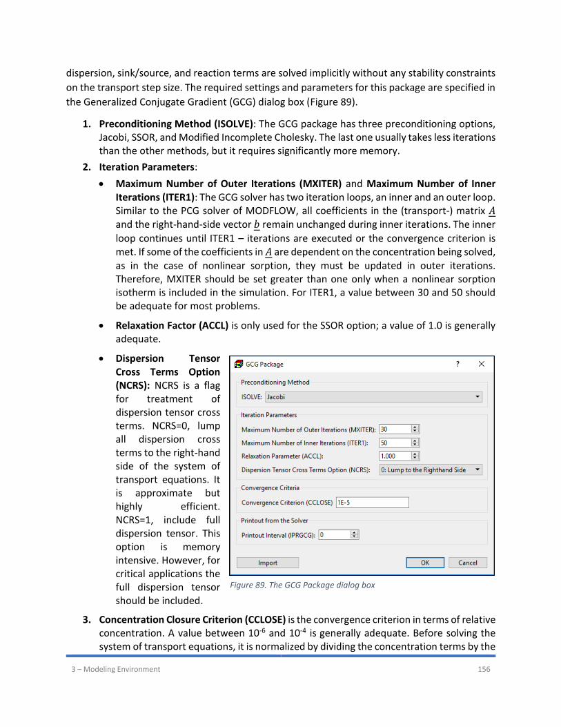
3 – Modeling Environment 156
dispersion, sink/source, and reaction terms are solved implicitly without any stability constraints
on the transport step size. The required settings and parameters for this package are specified in
the Generalized Conjugate Gradient (GCG) dialog box (Figure 89).
1. Preconditioning Method (ISOLVE): The GCG package has three preconditioning options, Jacobi, SSOR, and Modified Incomplete Cholesky. The last one usually takes less iterations than the other methods, but it requires significantly more memory.
2. Iteration Parameters:
• Maximum Number of Outer Iterations (MXITER) and Maximum Number of Inner Iterations (ITER1): The GCG solver has two iteration loops, an inner and an outer loop. Similar to the PCG solver of MODFLOW, all coefficients in the (transport-) matrix 𝐴 and the right-hand-side vector 𝑏 remain unchanged during inner iterations. The inner
loop continues until ITER1 – iterations are executed or the convergence criterion is met. If some of the coefficients in 𝐴 are dependent on the concentration being solved, as in the case of nonlinear sorption, they must be updated in outer iterations. Therefore, MXITER should be set greater than one only when a nonlinear sorption isotherm is included in the simulation. For ITER1, a value between 30 and 50 should be adequate for most problems.
• Relaxation Factor (ACCL) is only used for the SSOR option; a value of 1.0 is generally adequate.
• Dispersion Tensor Cross Terms Option (NCRS): NCRS is a flag for treatment of dispersion tensor cross terms. NCRS=0, lump all dispersion cross terms to the right-hand side of the system of transport equations. It is approximate but highly efficient. NCRS=1, include full dispersion tensor. This option is memory intensive. However, for critical applications the full dispersion tensor should be included.
3. Concentration Closure Criterion (CCLOSE) is the convergence criterion in terms of relative concentration. A value between 10-6 and 10-4 is generally adequate. Before solving the system of transport equations, it is normalized by dividing the concentration terms by the
Figure 89. The GCG Package dialog box

3 – Modeling Environment 157
maximum concentration of all cells. When the change of the normalized concentration at all cells during an inner iteration is less than or equal to CCLOSE, iteration stops. When it takes only one inner iteration to converge, the solution is considered to have converged and the simulation proceeds to the next transport step.
4. Printout Interval (IPRGCG): The maximum concentration changes are printed out whenever the iteration number is an even multiple of this printout interval. Set it to zero for printing only at the end of each stress period.
3.8.3.5. Output Control
The available options of the Output Control (MT3D/SEAWAT) dialog box are described as follows.
1. Output Options Tab (Figure 90)
• SAVUCN indicates whether the calculated concentration values should be saved in binary files which are used by PM for visualization. The default file names of the binary files are MT3Dnnn.UCN for the dissolved phase and MT3Dnnns.UCN for the sorbed phases, where nnn is the species number.
• IFMTCN indicates whether the calculated concentration values should be printed to the Run Listing file.
• IFMTNP indicates whether the number of particles in each cell should be printed to the Run Listing file.
• IFMTRF indicates whether the model-calculated retardation factor should be printed to the Run Listing file.
• IFMTDP indicates whether the model-calculated, distance weighted dispersion coefficient should be printed to the Run Listing File.
• CHKMAS indicates whether mass budget summary information should be printed to the mass budget file. The default file names of the mass budget summary files are MT3Dnnn.MAS, where nnn is the species number.
• NPRMAS: Mass budget summary information is printed every NPRMAS transport step, if CHKMAS is checked.
Figure 90. The Output Options tab of the Output Control (MT3D/SEAWAT) dialog box
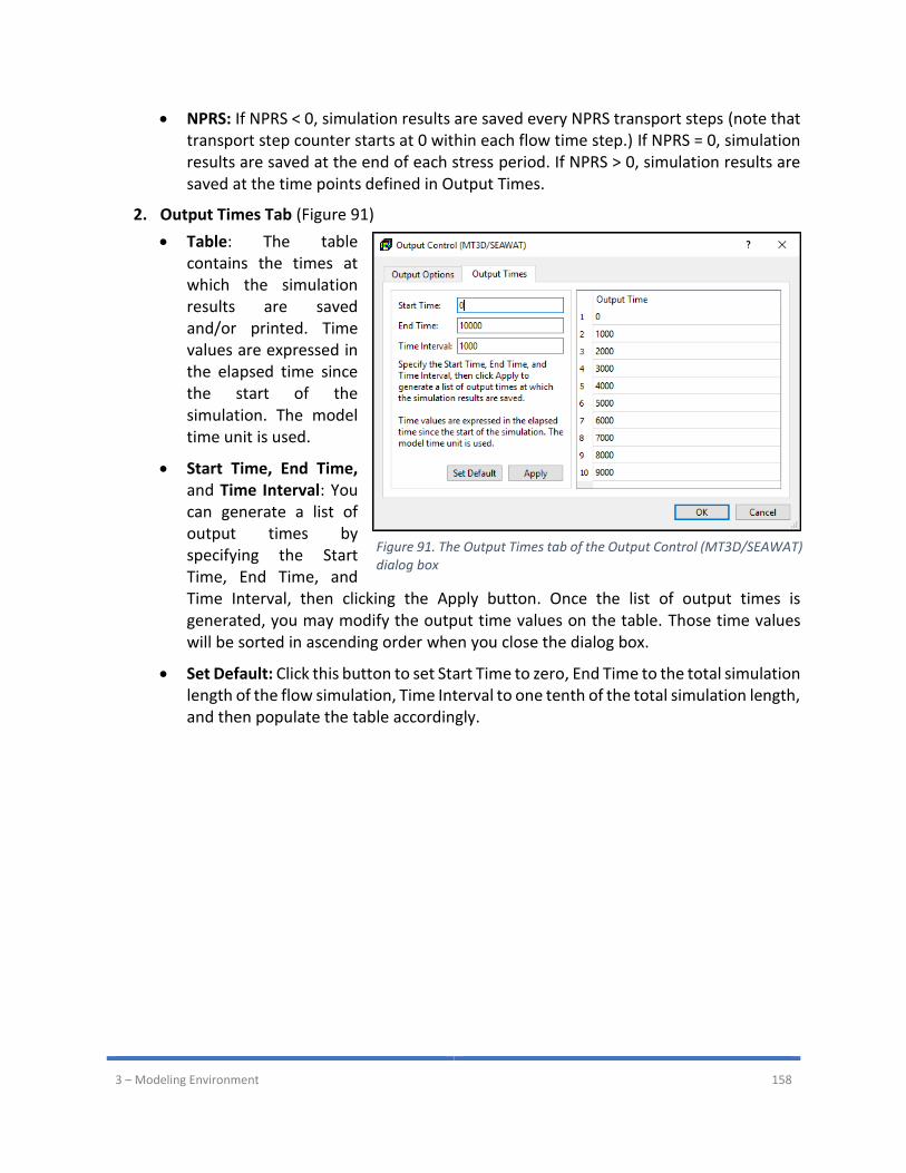
3 – Modeling Environment 158
• NPRS: If NPRS < 0, simulation results are saved every NPRS transport steps (note that transport step counter starts at 0 within each flow time step.) If NPRS = 0, simulation results are saved at the end of each stress period. If NPRS > 0, simulation results are saved at the time points defined in Output Times.
2. Output Times Tab (Figure 91)
• Table: The table contains the times at which the simulation results are saved and/or printed. Time values are expressed in the elapsed time since the start of the simulation. The model time unit is used.
• Start Time, End Time, and Time Interval: You can generate a list of output times by specifying the Start Time, End Time, and Time Interval, then clicking the Apply button. Once the list of output times is generated, you may modify the output time values on the table. Those time values will be sorted in ascending order when you close the dialog box.
• Set Default: Click this button to set Start Time to zero, End Time to the total simulation length of the flow simulation, Time Interval to one tenth of the total simulation length, and then populate the table accordingly.
Figure 91. The Output Times tab of the Output Control (MT3D/SEAWAT) dialog box

3 – Modeling Environment 159
3.8.3.6. Run
Select this menu item to open the Run MT3D dialog box (Figure 92) or Run SEAWAT dialog box
according to the transport model selected in the Transport Settings dialog box (Section 3.8.3.1).
The Run MT3D or Run SEAWAT dialog box can be used to start a transport simulation or to build
input files. The available settings of the dialog box are described below.
1. Table
• The build box. Prior to running a transport simulation, PM uses the user-specified data to build input files for MT3D (or SEAWAT). An input file will be built if its build box is checked. If an input file does not exist or the input data has been modified since the last build, its build box will be checked automatically.
• Package is the name of the package of the flow model.
• Filename is the name of the input file.
• Status shows the status (such as Ready, Not Exist, etc.) of the input file.
2. More Actions
• Inspect Model Data: Select this to check the correctness and consistency of the model data. The inspection report will be saved in the mt3d_inspection_log.txt or seawat_inspection_log.txt file.
• Build Input Files: Select this to build the input files with the checked build boxes. The name file mt3d.nam or seawat.nam will also be built. The build log is stored in the mt3d_build_log.txt or seawat_build_log.txt file.
• Rebuild All Input Files: Select this to rebuild all input files, except for existing input files that are marked as read-only. The build log is stored in the mt3d_build_log.txt or seawat__build_log.txt file.
3. Run: Click this button to build input files with the checked build boxes and the start the transport simulation.
Figure 92. The Run MT3D dialog box
3 – Modeling Environment 160
• If Constant Density Transport (MT3D) is selected as the transport model, the simulation will be carried out by MT3D.
• If Variable Density Flow and Transport (SEAWAT) is selected as the transport model, the simulation will be carried out by SEAWAT.
The transport simulation progress will be displayed in the MT3D or SEAWAT Output window. You may terminate the simulation at any time by clicking on the Terminate button.
3.8.3.7. View
Run Listing File
Select this menu item to use the Text Editor (see Section 3.4.11) to display the run listing file
mt3d.list or seawat.list.
Scatter Chart
Select View > Scatter Chart to display the scatter chart based on the concentration data of the
dissolved phase. The use of the Concentration Scatter Chart dialog box is identical as the Head
Scatter Chart dialog box (see Section 3.8.1.5.3), with the following exceptions:
1. Species dropdown box is displayed on the lower-left corner of the dialog box. Use this dropdown box to select a species of interest.
2. The simulated concentration data of the selected species is used in the Chart and the Data tab.
Line Chart
Select View > Line Chart to display the time-series chart based on the concentration data of the
dissolved phase. The use of the Concentration Line Chart dialog box is identical as the Head Line
Chart dialog box (see Section 3.8.1.5.4 ), with the following exceptions:
1. Species dropdown box is displayed on the lower-left corner of the dialog box. Use this dropdown box to select a species of interest.
2. The simulated concentration data of the selected species is used in the Chart and the Data tab.
Mass Budget Summary
Select this menu item, and then select a species to display the mass budget summary file of that
species. The default file names of the mass budget summary files are MT3Dnnn.MAS, where nnn
is the species number. Refer to (Neville, 2006) for details about interpreting the MT3D mass
budget.
Concentration Summary
Select this menu item, and then select a species to create a time-history of the average
concentration of the model. The calculation is based on the simulated concentration values
3 – Modeling Environment 161
(stored in the MT3Dnnn.ucn file, where nnn is the number of a species) and the water volume
(see Section 3.8.1.5.5 for details) of the model. The calculation results are stored in a comma-
separated value file consisting of a number of records. Each record includes the following terms.
• ElapsedTime is the elapsed time since the start of the simulation at which the simulated concentration values are stored in the MT3Dnnn.ucn file. Since the total amount of water in the model must be calculated as well, the average concentration will not be calculated for the ElapsedTime that does not lie between the date/time of the first and last head results.
• Period is the stress period where ElapsedTime belongs to.
• TimeStep is the time step within the given Period where ElapsedTime belongs to.
• Date is the calendar date in the form of year-month-day. The date corresponds to the given elapsed time.
• Volume [L3] is the total amount of water in the model. This value is calculated in the same way as the Volume described in Section 3.8.1.5.5.
• Mass [L3 x concentration unit] is the calculated as follows.
𝑀𝑎𝑠𝑠 = ∑ (𝑣𝑠𝑖 + 𝑣𝑠𝑦𝑖) × 𝑐𝑖
𝑛
𝑖=0
where
𝑛 is the total number of model cells,
𝑐𝑖 is the solute concentration of the selected species in the ith cell at the given elapsed time,
𝑣𝑠𝑖 is the volume of water stored in the ith cell due to compressibility, and
𝑣𝑠𝑦𝑖 is the volume of water stored in the pore space of the ith cell.
The values of 𝑣𝑠𝑖 and 𝑣𝑠𝑦𝑖 are calculated in the same way as described in Section 3.8.1.5.5. It is assumed that 𝑣𝑠𝑖 and 𝑣𝑠𝑦𝑖 have the same concentration 𝑐𝑖.
• Concentration is calculated as Mass/Volume, and has the same unit as your input concentration values.
Production Concentration Summary
Select this menu item, and then select a species to create a time-history of the concentration of
the extracted groundwater at the pumping wells. The calculation is based on the simulated
concentration values (stored in the MT3Dnnn.ucn file, where nnn is the number of a species) and
the pumping rates (stored in the modflow.flow file) at well cells. The calculation results are stored
in a comma-separated value file consisting of a number of records. Each record includes the
following terms.
3 – Modeling Environment 162
• ElapsedTime is the elapsed time since the start of the simulation at which the simulated concentration values are stored in the MT3Dnnn.ucn file. Since the total amount of water in the model must be calculated as well, the average concentration will not be calculated for the ElapsedTime that does not lie between the date/time of the first and last flow results.
• Period is the stress period where ElapsedTime belongs to.
• TimeStep is the time step within the given Period where ElapsedTime belongs to.
• Date is the calendar date in the form of year-month-day. The date corresponds to the given elapsed time.
• Well is the well name. The cells with the same well name will be considered a part of the well. If the well name of a well cell is not specified, the default name “row_column” will be used, where row/column are the model row and column of the well cell. Consequently, the cells in various layers of that row/column location will be considered a part of that well.
• PumpingRate [L3/T] is the sum of the pumping rates of the model cells that belong to the given well.
• MassRate [L3/T x concentration unit] is the sum of [pumping rate x concentration] of the model cells that belong to the given well.
• Concentration is the concentration of the water extracted by the well. The value is calculated as [Concentration = MassRate / PumpingRate] and has the same unit as your input concentration values.
3.8.4. PEST
This menu provides the interface to PEST (Doherty, 2016) and/or BeoPEST (Hunt, et al., 2010).
Table 4 shows a list of estimable parameters through PEST or BEOPEST within PM. The estimable
aquifer parameters depend on the selection of the internal flow package and layer types32. During
a parameter estimation process, PEST searches optimum parameter values for which the sum of
squared deviations between model-calculated and observed values at the observation points is
reduced to a minimum.
1. To define observation points and observation values
• See Section 3.5.3 for details.
2. To define an estimable parameter
• Select a parameter from the Parameters menu or select a package from Models > MODFLOW > Packages menu
32 When BCF is selected as the internal flow package, the estimable aquifer parameters depend on the layer type (as listed in Table 3) regardless of the Calculated/User-specified settings in the Layer Property dialog box.

3 – Modeling Environment 163
• Assign an initial guess of the parameter value and a parameter number to cells within an area where the parameter value should be estimated.
o The initial guess of the parameter value must be non-zero.
o The parameter number must be unique within a parameter type (e.g., T, S or Ss)
and may be any integer ranging between 0 and 10000. Set the parameter number
to zero, if the specified parameter value should not be estimated.
• Select Model > PEST > Settings to open the PEST Settings dialog box. If this dialog box is opened the first time, the defined parameters will be listed in the Parameters Tab. Otherwise, select More Actions > Search for Parameters to find the new parameters.
Table 4. Estimable Parameters through PEST/BeoPEST within PM
3.8.4.1. Settings
The required inputs and options for running PEST and/or BeoPEST are specified in the PEST
Settings dialog box (Figure 93). The variable names used in this dialog box are identical as those
given in the PEST Manual (Doherty, 2016). Briefly explanations of these variables are provided
below. Consult the PEST Manual for details.
1. Operation Mode
33 VCONT is used only if the layer is not the bottom layer.
Packages Parameters
Block-Centered Flow (BCF) Confined: T, S, and VCONT33 Unconfined: HK, Sy, and VCONT33 Limited Convertible: T, S, Sy, and VCONT33 Full Convertible: HK, S, Sy, and VCONT33
Layer-Property Flow (LPF) All layer types: HK, HANI, VANI, VK, Ss, and Sy.
Upstream-Weighting (UPW) All layer types: HK, HANI, VANI, VK, Ss, and Sy.
Drain (DRN) Drain conductance
Drain with Return Flow (DRT) Drain conductance
Evapotranspiration (EVT) Maximum ET Flux
Evapotranspiration Segments (ETS) Maximum ET Flux
General-Head Boundary (GHB) Boundary conductance
Horizontal-Flow Barrier (HBF) Hydraulic characteristic
Interbed Storage (IBS) Inelastic Storage Factor
Recharge (RCH) Recharge flux
River (RIV) Riverbed conductance
Reservoir (RES1) Vertical hydraulic conductivity of reservoir bed
Stream (STR) Streambed conductance
Unsaturated-Zone Flow (UZF1) Infiltration rate
Well (WEL) Flow rate
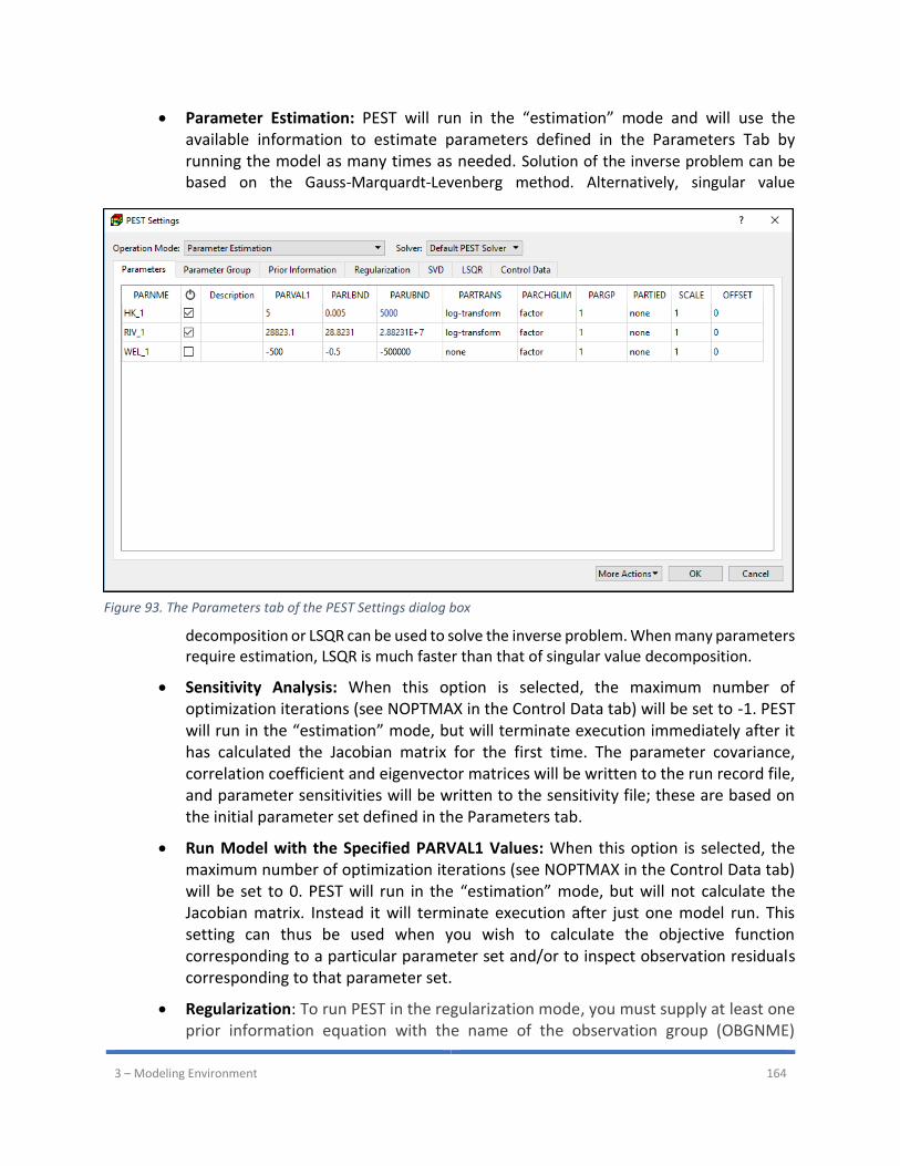
3 – Modeling Environment 164
• Parameter Estimation: PEST will run in the “estimation” mode and will use the available information to estimate parameters defined in the Parameters Tab by running the model as many times as needed. Solution of the inverse problem can be based on the Gauss-Marquardt-Levenberg method. Alternatively, singular value
decomposition or LSQR can be used to solve the inverse problem. When many parameters require estimation, LSQR is much faster than that of singular value decomposition.
• Sensitivity Analysis: When this option is selected, the maximum number of optimization iterations (see NOPTMAX in the Control Data tab) will be set to -1. PEST will run in the “estimation” mode, but will terminate execution immediately after it has calculated the Jacobian matrix for the first time. The parameter covariance, correlation coefficient and eigenvector matrices will be written to the run record file, and parameter sensitivities will be written to the sensitivity file; these are based on the initial parameter set defined in the Parameters tab.
• Run Model with the Specified PARVAL1 Values: When this option is selected, the maximum number of optimization iterations (see NOPTMAX in the Control Data tab) will be set to 0. PEST will run in the “estimation” mode, but will not calculate the Jacobian matrix. Instead it will terminate execution after just one model run. This setting can thus be used when you wish to calculate the objective function corresponding to a particular parameter set and/or to inspect observation residuals corresponding to that parameter set.
• Regularization: To run PEST in the regularization mode, you must supply at least one prior information equation with the name of the observation group (OBGNME)
Figure 93. The Parameters tab of the PEST Settings dialog box
3 – Modeling Environment 165
starting with “regul”. As described in (Doherty, 2016), when run in “regularization” mode, PEST employs two objective functions rather than one. One of these is called the “measurement objective function” while the other is referred to as the “regularization objective function”. The lower is the former, the better do model-calculated quantities match their field-measured counterparts. The lower is the latter, the better do parameter values respect mathematical expressions of expert knowledge encapsulated in observations or prior information equations that are dedicated to this purpose. Refer to the PEST book (Doherty, 2015) and Chapter 9 of the Part I of the PEST Manual (Doherty, 2016) for details about the regularization mode.
2. Solver: The selected solver is used to solve the linearized inverse problem during each iteration of the overall inverse process. As discussed in (Doherty, 2015), the Singular value decomposition (SVD) and the LSQR algorithm introduce numerical stability to solution of an ill-posed inverse problem. In most cases, SVD Mode1, SVD Mode 2, or LSQR should be used instead of the PEST’s default solver. SVD Mode 2 is superior than SVD Mode 1 for cases involving many observations as the formation of the matrix for the inverse problem may take a considerable amount of time under these circumstances. A benefit of LSQR over SVD is its speed. If parameters number more than a couple of thousand, SVD can become very slow. This is not the case for LSQR which can happily handle tens of thousands of parameters and hundreds of thousands of observations.
3. More Actions: This menu acts on the Parameter Table (see below), the functions of the menu items are as follows.
• Update: Update PARVAL1 of the Parameter Table with the estimated parameter values.
• Delete: Delete the selected row from the Parameter Table.
• Clean Up: Delete unused parameters from the Parameter Tab. An estimable parameter becomes unused when its parameter number no longer exists in all cells of the respective parameter type.
• Search for Parameters: Search for estimable parameters and add them to the Parameter Tab.
4. Parameters Tab contains a Parameter Table that lists the estimable parameters and their properties.
• PARNAM is the parameter name and is a combination of that parameter number and the short name of the aquifer parameter (i.e., HK, HANI, VK, VANI, SS, SY, T, S or VCONT) or package. For example, if parameter numbers 1 and 2 are specified for the Recharge Package, the parameter names are RCH_1 and RCH_2. Similarly, if parameter numbers 3 is assigned to HK, the parameter name is HK_3. Modification of the parameter names is not allowed. Note that when switching between internal flow packages (i.e., BCF, LPF, and UPW), some aquifer parameters might become
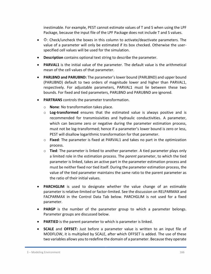
3 – Modeling Environment 166
inestimable. For example, PEST cannot estimate values of T and S when using the LPF Package, because the input file of the LPF Package does not include T and S values.
• : Check/uncheck the boxes in this column to activate/deactivate parameters. The value of a parameter will only be estimated if its box checked. Otherwise the user-specified cell values will be used for the simulation.
• Description contains optional text string to describe the parameter.
• PARVAL1 is the initial value of the parameter. The default value is the arithmetical mean of the cell values of that parameter.
• PARLBND and PARUBND: The parameter’s lower bound (PARLBND) and upper bound (PARUBND) default to two orders of magnitude lower and higher than PARVAL1, respectively. For adjustable parameters, PARVAL1 must lie between these two bounds. For fixed and tied parameters, PARLBND and PARUBND are ignored.
• PARTRANS controls the parameter transformation.
o None: No transformation takes place.
o Log-transformed ensures that the estimated value is always positive and is
recommended for transmissivities and hydraulic conductivities. A parameter,
which can become zero or negative during the parameter estimation process,
must not be log-transformed; hence if a parameter’s lower bound is zero or less,
PEST will disallow logarithmic transformation for that parameter.
o Fixed: The parameter is fixed at PARVAL1 and takes no part in the optimization
process.
o Tied: The parameter is linked to another parameter. A tied parameter plays only
a limited role in the estimation process. The parent parameter, to which the tied
parameter is linked, takes an active part in the parameter estimation process and
must be neither fixed nor tied itself. During the parameter estimation process, the
value of the tied parameter maintains the same ratio to the parent parameter as
the ratio of their initial values.
• PARCHGLIM is used to designate whether the value change of an estimable parameter is relative-limited or factor-limited. See the discussion on RELPARMAX and FACPARMAX in the Control Data Tab below. PARCHGLIM is not used for a fixed parameter.
• PARGP is the number of the parameter group to which a parameter belongs. Parameter groups are discussed below.
• PARTIED is the parent parameter to which is parameter is linked.
• SCALE and OFFSET: Just before a parameter value is written to an input file of MODFLOW, it is multiplied by SCALE, after which OFFSET is added. The use of these two variables allows you to redefine the domain of a parameter. Because they operate
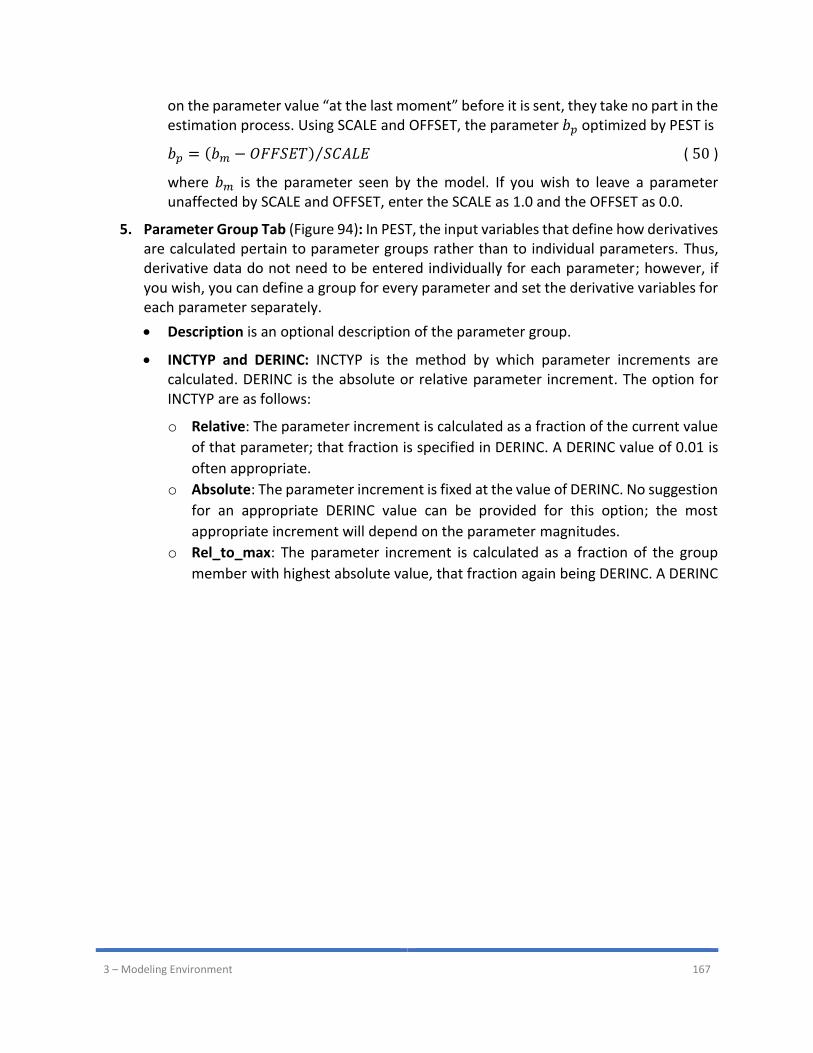
3 – Modeling Environment 167
on the parameter value “at the last moment” before it is sent, they take no part in the estimation process. Using SCALE and OFFSET, the parameter 𝑏𝑝 optimized by PEST is
𝑏𝑝 = (𝑏𝑚 − 𝑂𝐹𝐹𝑆𝐸𝑇) 𝑆𝐶𝐴𝐿𝐸⁄ ( 50 )
where 𝑏𝑚 is the parameter seen by the model. If you wish to leave a parameter unaffected by SCALE and OFFSET, enter the SCALE as 1.0 and the OFFSET as 0.0.
5. Parameter Group Tab (Figure 94): In PEST, the input variables that define how derivatives are calculated pertain to parameter groups rather than to individual parameters. Thus, derivative data do not need to be entered individually for each parameter; however, if you wish, you can define a group for every parameter and set the derivative variables for each parameter separately.
• Description is an optional description of the parameter group.
• INCTYP and DERINC: INCTYP is the method by which parameter increments are calculated. DERINC is the absolute or relative parameter increment. The option for INCTYP are as follows:
o Relative: The parameter increment is calculated as a fraction of the current value
of that parameter; that fraction is specified in DERINC. A DERINC value of 0.01 is
often appropriate.
o Absolute: The parameter increment is fixed at the value of DERINC. No suggestion
for an appropriate DERINC value can be provided for this option; the most
appropriate increment will depend on the parameter magnitudes.
o Rel_to_max: The parameter increment is calculated as a fraction of the group
member with highest absolute value, that fraction again being DERINC. A DERINC

3 – Modeling Environment 168
value of 0.01 is often appropriate. If a group contains members, which are fixed
and/or tied, the values of these parameters are used when calculating parameter
increments.
• DERINCLB is the lower bound of relative parameter increment; ignored if INCTYP is Absolute. If a parameter increment is calculated as Relative, it may become too low if the parameter values become very small. And, if a parameter increment is calculated as Rel_to_max, it may become too low if the modulus of the largest parameter in the group is very small. A parameter increment becomes “too low” if it does not allow reliable derivatives to be calculated with respect to that parameter because of round off errors incurred in the subtraction of nearly equal model generated values. DERINCLB is used to bypass this possibility. Set DERINCLB to zero if you do not wish to place a lower limit on parameter increments in this fashion.
• FORCEN determines whether higher order derivatives calculation is undertaken.
o Always_2: Derivatives will be calculated using the forward difference method.
o Always_3: PEST will use the central (i.e. three-point) method to calculate the
derivatives. In this case, twice as many model runs as there are parameters within
the group will be required. However, the derivatives will be calculated with
greater accuracy and this will probably have a beneficial effect on the
performance of PEST.
o Always_5: PEST will use a five-point method to calculate the derivatives.
o Switch: Derivatives calculations will begin using the forward difference method,
switching to the central (i.e. three-point) method for the remainder of the
Figure 94. The Parameter Group tab of the PEST Settings dialog box
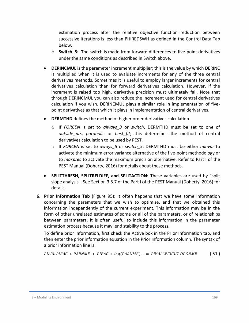
3 – Modeling Environment 169
estimation process after the relative objective function reduction between
successive iterations is less than PHIREDSWH as defined in the Control Data Tab
below.
o Switch_5: The switch is made from forward differences to five-point derivatives
under the same conditions as described in Switch above.
• DERINCMUL is the parameter increment multiplier; this is the value by which DERINC is multiplied when it is used to evaluate increments for any of the three central derivatives methods. Sometimes it is useful to employ larger increments for central derivatives calculation than for forward derivatives calculation. However, if the increment is raised too high, derivative precision must ultimately fall. Note that through DERINCMUL you can also reduce the increment used for central derivatives calculation if you wish. DERINCMUL plays a similar role in implementation of five-point derivatives as that which it plays in implementation of central derivatives.
• DERMTHD defines the method of higher order derivatives calculation.
o If FORCEN is set to always_3 or switch, DERMTHD must be set to one of
outside_pts, parabolic or best_fit; this determines the method of central
derivatives calculation to be used by PEST.
o If FORCEN is set to aways_5 or switch_5, DERMTHD must be either minvar to
activate the minimum error variance alternative of the five-point methodology or
to maxprec to activate the maximum precision alternative. Refer to Part I of the
PEST Manual (Doherty, 2016) for details about these methods.
• SPLITTHRESH, SPLITRELDIFF, and SPLITACTION: These variables are used by “split slope analysis”. See Section 3.5.7 of the Part I of the PEST Manual (Doherty, 2016) for details.
6. Prior Information Tab (Figure 95): It often happens that we have some information concerning the parameters that we wish to optimize, and that we obtained this information independently of the current experiment. This information may be in the form of other unrelated estimates of some or all of the parameters, or of relationships between parameters. It is often useful to include this information in the parameter estimation process because it may lend stability to the process.
To define prior information, first check the Active box in the Prior Information tab, and then enter the prior information equation in the Prior Information column. The syntax of a prior information line is
𝑃𝐼𝐿𝐵𝐿 𝑃𝐼𝐹𝐴𝐶 ∗ 𝑃𝐴𝑅𝑁𝑀𝐸 + 𝑃𝐼𝐹𝐴𝐶 ∗ 𝑙𝑜𝑔(𝑃𝐴𝑅𝑁𝑀𝐸) . . . = 𝑃𝐼𝑉𝐴𝐿 𝑊𝐸𝐼𝐺𝐻𝑇 𝑂𝐵𝐺𝑁𝑀𝐸 ( 51 )
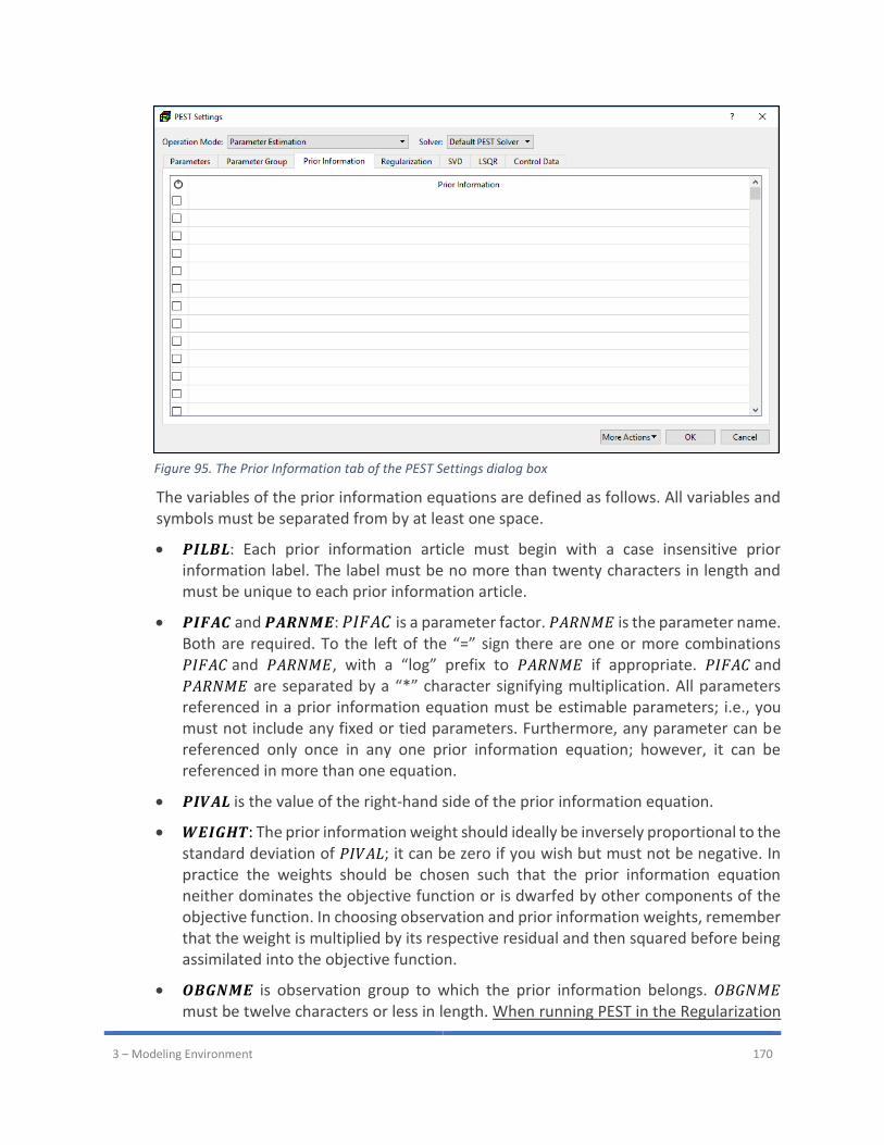
3 – Modeling Environment 170
The variables of the prior information equations are defined as follows. All variables and symbols must be separated from by at least one space.
• 𝑷𝑰𝑳𝑩𝑳: Each prior information article must begin with a case insensitive prior information label. The label must be no more than twenty characters in length and must be unique to each prior information article.
• 𝑷𝑰𝑭𝑨𝑪 and 𝑷𝑨𝑹𝑵𝑴𝑬: 𝑃𝐼𝐹𝐴𝐶 is a parameter factor. 𝑃𝐴𝑅𝑁𝑀𝐸 is the parameter name. Both are required. To the left of the “=” sign there are one or more combinations 𝑃𝐼𝐹𝐴𝐶 and 𝑃𝐴𝑅𝑁𝑀𝐸, with a “log” prefix to 𝑃𝐴𝑅𝑁𝑀𝐸 if appropriate. 𝑃𝐼𝐹𝐴𝐶 and 𝑃𝐴𝑅𝑁𝑀𝐸 are separated by a “*” character signifying multiplication. All parameters referenced in a prior information equation must be estimable parameters; i.e., you must not include any fixed or tied parameters. Furthermore, any parameter can be referenced only once in any one prior information equation; however, it can be referenced in more than one equation.
• 𝑷𝑰𝑽𝑨𝑳 is the value of the right-hand side of the prior information equation.
• 𝑾𝑬𝑰𝑮𝑯𝑻: The prior information weight should ideally be inversely proportional to the standard deviation of 𝑃𝐼𝑉𝐴𝐿; it can be zero if you wish but must not be negative. In practice the weights should be chosen such that the prior information equation neither dominates the objective function or is dwarfed by other components of the objective function. In choosing observation and prior information weights, remember that the weight is multiplied by its respective residual and then squared before being assimilated into the objective function.
• 𝑶𝑩𝑮𝑵𝑴𝑬 is observation group to which the prior information belongs. 𝑂𝐵𝐺𝑁𝑀𝐸 must be twelve characters or less in length. When running PEST in the Regularization
Figure 95. The Prior Information tab of the PEST Settings dialog box
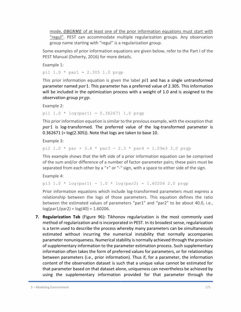
3 – Modeling Environment 171
mode, 𝑂𝐵𝐺𝑁𝑀𝐸 of at least one of the prior information equations must start with “regul”. PEST can accommodate multiple regularization groups. Any observation group name starting with “regul” is a regularization group.
Some examples of prior information equations are given below, refer to the Part I of the PEST Manual (Doherty, 2016) for more details.
Example 1:
pi1 1.0 * par1 = 2.305 1.0 prgp
This prior information equation is given the label 𝑝𝑖1 and has a single untransformed parameter named 𝑝𝑎𝑟1. This parameter has a preferred value of 2.305. This information will be included in the optimization process with a weight of 1.0 and is assigned to the observation group 𝑝𝑟𝑔𝑝.
Example 2:
pi1 1.0 * log(par1) = 0.362671 1.0 prgp
This prior information equation is similar to the previous example, with the exception that 𝑝𝑎𝑟1 is log-transformed. The preferred value of the log-transformed parameter is 0.362671 (= log(2.305)). Note that logs are taken to base 10.
Example 3:
pi2 1.0 * par + 3.4 * par3 - 2.3 * par4 = 1.09e3 3.0 prgp
This example shows that the left side of a prior information equation can be comprised of the sum and/or difference of a number of factor-parameter pairs; these pairs must be separated from each other by a “+” or “-“ sign, with a space to either side of the sign.
Example 4:
pi3 1.0 * log(par1) - 1.0 * log(par2) = 1.60206 2.0 prgp
Prior information equations which include log-transformed parameters must express a relationship between the logs of those parameters. This equation defines the ratio between the estimated values of parameters “par1” and “par2” to be about 40.0, i.e., log(par1/par2) = log(40) = 1.60206.
7. Regularization Tab (Figure 96): Tikhonov regularization is the most commonly used method of regularization and is incorporated in PEST. In its broadest sense, regularization is a term used to describe the process whereby many parameters can be simultaneously estimated without incurring the numerical instability that normally accompanies parameter nonuniqueness. Numerical stability is normally achieved through the provision of supplementary information to the parameter estimation process. Such supplementary information often takes the form of preferred values for parameters, or for relationships between parameters (i.e., prior information). Thus if, for a parameter, the information content of the observation dataset is such that a unique value cannot be estimated for that parameter based on that dataset alone, uniqueness can nevertheless be achieved by using the supplementary information provided for that parameter through the
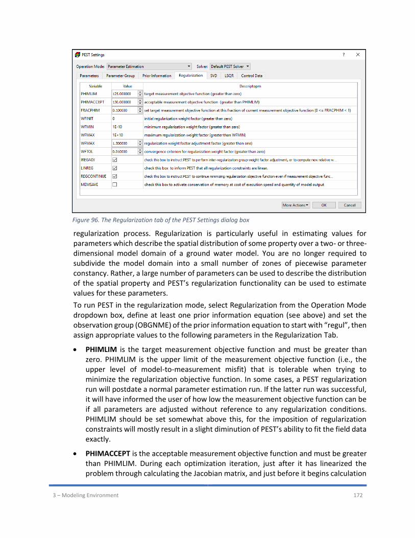
3 – Modeling Environment 172
regularization process. Regularization is particularly useful in estimating values for parameters which describe the spatial distribution of some property over a two- or three-dimensional model domain of a ground water model. You are no longer required to subdivide the model domain into a small number of zones of piecewise parameter constancy. Rather, a large number of parameters can be used to describe the distribution of the spatial property and PEST’s regularization functionality can be used to estimate values for these parameters.
To run PEST in the regularization mode, select Regularization from the Operation Mode dropdown box, define at least one prior information equation (see above) and set the observation group (OBGNME) of the prior information equation to start with “regul”, then assign appropriate values to the following parameters in the Regularization Tab.
• PHIMLIM is the target measurement objective function and must be greater than zero. PHIMLIM is the upper limit of the measurement objective function (i.e., the upper level of model-to-measurement misfit) that is tolerable when trying to minimize the regularization objective function. In some cases, a PEST regularization run will postdate a normal parameter estimation run. If the latter run was successful, it will have informed the user of how low the measurement objective function can be if all parameters are adjusted without reference to any regularization conditions. PHIMLIM should be set somewhat above this, for the imposition of regularization constraints will mostly result in a slight diminution of PEST’s ability to fit the field data exactly.
• PHIMACCEPT is the acceptable measurement objective function and must be greater than PHIMLIM. During each optimization iteration, just after it has linearized the problem through calculating the Jacobian matrix, and just before it begins calculation
Figure 96. The Regularization tab of the PEST Settings dialog box
3 – Modeling Environment 173
of the parameter upgrade vector, PEST calculates the optimal value of the regularization weight factor for that iteration. This is the value which, under the linearity assumption encapsulated in the Jacobian matrix, results in a parameter upgrade vector for which the measurement component of the objective function is equal to PHIMLIM. However, due to the approximate nature of the linearity assumption, PEST may not be able to lower the measurement component of the objective function to PHIMLIM on that iteration although it uses several different values for the Marquardt lambda in attempting to do so. If it cannot lower the measurement objective function to an acceptable level, it simply accepts the upgraded parameters, proceeds to the next optimization iteration. However, if it does succeed in lowering the measurement objective function to an acceptable level, or if it has succeeded in doing this on previous iterations, then PEST slightly alters its philosophy of choosing new Marquardt lambdas, in that it now attempts to lower the regularization component of the objective function while maintaining the measurement component of the objective function below this acceptable level. This acceptable level is PHIMACCEPT; it should be set slightly higher than PHIMLIM so that PEST has some room to move.
• FRACPHIM set target measurement objective function at this fraction of current measurement objective function (0 ≤ FRACPHIM < 1).
• WFINIT is the initial regularization weight factor and must be greater than zero. During every optimization iteration PEST calculates a suitable regularization weight factor using an iterative, numerical solution procedure; its initial value for the first optimization iteration is WFINIT.
• WFMIN and WFMAX are respectively the minimum and maximum regularization weight factors and must be greater than zero. If a regularization scheme is poor, (and does not lend too much stability to an already unstable parameter estimation process), selection of appropriate values for WFMIN and WFMAX may be quite important, for these can prevent PEST from calculating outrageous values for the regularization weight factor to compensate for inadequacies of the regularization scheme.
• WFFAC and WFTOL. WFFAC is the regularization weight factor adjustment factor and must be greater than one. WFTOL is the convergence criterion for regularization weight factor and must be greater than zero. When PEST calculates the appropriate regularization weight factor to use during an optimization iteration, it uses an iterative procedure which begins at the value of the regularization weight factor calculated for the previous optimization iteration; for the first iteration, it uses WFINIT to start the procedure. In the process of finding the weight factor, PEST first travels along a path of progressively increasing or decreasing weight factor by either multiplying or dividing the weight factor by WFFAC; it continues to do this until it has found two successive weight factors which lie on either side of the optimal weight factor for that optimization iteration. Once it has done this, it uses Newtons method to calculate the
3 – Modeling Environment 174
optimal weight factor, through a series of successive approximations. When two subsequent weight factors calculated in this way differ from each other by no more than a relative amount of WFTOL, the optimal weight factor is deemed to have been calculated.
• IREGADJ: Check this box to instruct PEST to perform inter-regularization group weight factor adjustment, or to compute new relative weights for regularization observations and prior information equations
• LINREG: Check this box to inform PEST that all regularization constraints are linear. As discussed in the PEST Manual, regularization constraints can be supplied through observations, through prior information, or both. Prior information relationships are always linear. Regularization constraints supplied as observations (for which the current value of pertinent relationships is calculated by the model), can be linear or nonlinear; in either case, derivatives of these relationships with respect to adjustable parameters are re-evaluated by PEST during each optimization iteration. If regularization information is entirely linear, many matrix operations carried out as part of PEST’s regularization functionality do not need to be repeated from iteration to iteration. If repetition of these calculations can be avoided in parameter estimation contexts involving many regularization constraints, significant gains in efficiency can be made.
• REGCONTINUE: Check this box to instruct PEST to continue minimizing regularization objective function even if measurement objective function less than PHIMLIM. Under normal circumstances, when working in regularization mode, PEST ceases execution immediately if the measurement objective function falls below PHIMLIM. There are some circumstances, however, where minimization of the regularization objective function is just as important as allowing the measurement objective function to reach PHIMLIM. If this box is checked, PEST will continue optimizing regularization objective function after reached PHIMLIM.
• MEMSAVE: Check this box to activate conservation of memory at cost of execution speed and quantity of model output. If this box is checked, nonessential PEST tasks which are curtailed include the following:
o The parameter covariance matrix, and matrices derived from it, are not calculated
by PEST at regular intervals during the parameter estimation process for recording
in the matrix file, pest.mtt; nor are these matrices calculated at the end of the
inversion process for recording in the run record file pest.rec. Because the
covariance matrix is unavailable, parameter uncertainties cannot be calculated,
and hence are also not recorded in the run record file. (In a regularization context,
these have little meaning anyway.)
o Some avenues for increasing the efficiency of regularization calculations are no
longer available under the leaner storage regime that prevails when memory
conservation is active (including the benefits gained through the LINREG variable
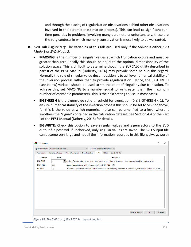
3 – Modeling Environment 175
and through the placing of regularization observations behind other observations
involved in the parameter estimation process). This can lead to significant run-
time penalties in problems involving many parameters; unfortunately, these are
the very contexts in which memory conservation is most likely to be warranted.
8. SVD Tab (Figure 97): The variables of this tab are used only if the Solver is either SVD Mode 1 or SVD Mode 2.
• MAXSING is the number of singular values at which truncation occurs and must be greater than zero. Ideally this should be equal to the optimal dimensionality of the solution space. This is difficult to determine though the SUPCALC utility described in part II of the PEST Manual (Doherty, 2016) may provide some help in this regard. Normally the role of singular value decomposition is to achieve numerical stability of the inversion process rather than to provide regularization. Hence, the EIGTHRESH (see below) variable should be used to set the point of singular value truncation. To achieve this, set MAXSING to a number equal to, or greater than, the maximum number of estimable parameters. This is the best setting to use in most cases.
• EIGTHRESH is the eigenvalue ratio threshold for truncation (0 ≤ EIGTHRESH < 1). To ensure numerical stability of the inversion process this should be set to 5E-7 or above, for this is the value at which numerical noise can be amplified to a level where it smothers the “signal” contained in the calibration dataset. See Section 4.4 of the Part I of the PEST Manual (Doherty, 2016) for details.
• EIGWRITE: Check this option to save singular values and eigenvectors to the SVD output file pest.svd. If unchecked, only singular values are saved. The SVD output file can become very large and not all the information recorded in this file is always worth
Figure 97. The SVD tab of the PEST Settings dialog box
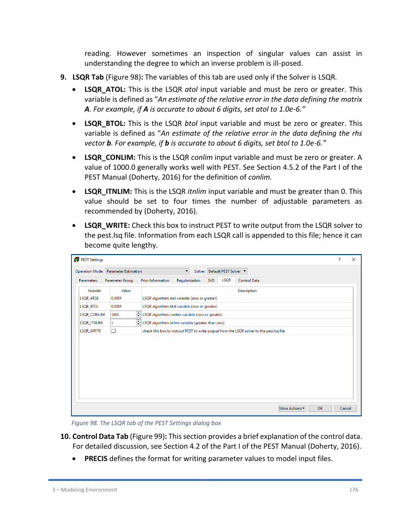
3 – Modeling Environment 176
reading. However sometimes an inspection of singular values can assist in understanding the degree to which an inverse problem is ill-posed.
9. LSQR Tab (Figure 98): The variables of this tab are used only if the Solver is LSQR.
• LSQR_ATOL: This is the LSQR atol input variable and must be zero or greater. This variable is defined as “An estimate of the relative error in the data defining the matrix A. For example, if A is accurate to about 6 digits, set atol to 1.0e-6.”
• LSQR_BTOL: This is the LSQR btol input variable and must be zero or greater. This variable is defined as “An estimate of the relative error in the data defining the rhs vector b. For example, if b is accurate to about 6 digits, set btol to 1.0e-6.”
• LSQR_CONLIM: This is the LSQR conlim input variable and must be zero or greater. A value of 1000.0 generally works well with PEST. See Section 4.5.2 of the Part I of the PEST Manual (Doherty, 2016) for the definition of conlim.
• LSQR_ITNLIM: This is the LSQR itnlim input variable and must be greater than 0. This value should be set to four times the number of adjustable parameters as recommended by (Doherty, 2016).
• LSQR_WRITE: Check this box to instruct PEST to write output from the LSQR solver to the pest.lsq file. Information from each LSQR call is appended to this file; hence it can become quite lengthy.
10. Control Data Tab (Figure 99): This section provides a brief explanation of the control data. For detailed discussion, see Section 4.2 of the Part I of the PEST Manual (Doherty, 2016).
• PRECIS defines the format for writing parameter values to model input files.
Figure 98. The LSQR tab of the PEST Settings dialog box
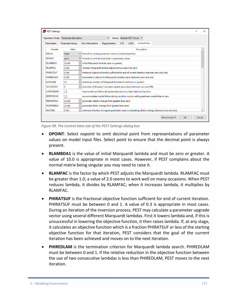
3 – Modeling Environment 177
• DPOINT: Select nopoint to omit decimal point from representations of parameter values on model input files. Select point to ensure that the decimal point is always present.
• RLAMBDA1 is the value of initial Marquardt lambda and must be zero or greater. A value of 10.0 is appropriate in most cases. However, if PEST complains about the normal matrix being singular you may need to raise it.
• RLAMFAC is the factor by which PEST adjusts the Marquardt lambda. RLAMFAC must be greater than 1.0; a value of 2.0 seems to work well on many occasions. When PEST reduces lambda, it divides by RLAMFAC; when it increases lambda, it multiplies by RLAMFAC.
• PHIRATSUF is the fractional objective function sufficient for end of current iteration. PHIRATSUF must be between 0 and 1. A value of 0.3 is appropriate in most cases. During an iteration of the inversion process, PEST may calculate a parameter upgrade vector using several different Marquardt lambdas. First it lowers lambda and, if this is unsuccessful in lowering the objective function, it then raises lambda. If, at any stage, it calculates an objective function which is a fraction PHIRATSUF or less of the starting objective function for that iteration, PEST considers that the goal of the current iteration has been achieved and moves on to the next iteration.
• PHIREDLAM is the termination criterion for Marquardt lambda search. PHIREDLAM must be between 0 and 1. If the relative reduction in the objective function between the use of two consecutive lambdas is less than PHIREDLAM, PEST moves to the next iteration.
Figure 99. The Control Data tab of the PEST Settings dialog box
3 – Modeling Environment 178
• NUMLAM is the maximum number of Marquardt lambdas to test during an iteration. NUMLAM must be 1 or greater and should normally be set to 10.
• JACUPDATE is used in conjunction with the activation of Broyden’s Jacobian update procedure, which provides a mechanism for improving the Jacobian matrix based on model outputs calculated during model runs undertaken for testing parameter upgrades calculated using different values of the Marquardt lambda.
o If it is set to zero, Broyden updating of the Jacobian matrix does not occur.
o If it is set to 999, Jacobian matrix is updated after the first parameter upgrade
attempt, and every parameter upgrade attempt thereafter.
o If it is set to n, where 0 < n < 999, Broyden updating will be undertaken during a
PEST iteration following the first n attempts to upgrade parameters using n
different values of the Marquardt lambdas.
• LAMFORGIVE treats model run failure during lambda search as high objective function.
o If this box is unchecked: when a model fails to run to completion during a
parameter estimation process, PEST reports this error condition and ceases
execution with an error message.
o If this box is checked: when a model fails to run to completion during a parameter
estimation process, PEST ignores the failed model run and attempts new sets of
parameters using other values of the Marquardt lambda. If it failed to find
parameters that allow the model to complete execution, PEST either switches to
central derivatives calculation or ceases execution with an appropriate error
message.
• DERFORGIVE plays a similar role to LAMFORGIVE. However, DERFORGIVE governs PEST’s behavior when model runs are being undertaken for finite-difference derivatives calculation. If this box is checked, DERFORGIVE accommodates model failure during Jacobian runs by setting pertinent sensitivities to zero.
• RELPARMAX is the maximum relative change that a parameter may undergo between optimization iterations. RELPARMAX must be greater than zero.
• FACPARMAX is the maximum factor change that a parameter may undergo between optimization iterations. FACPARMAX must be greater than zero.
• FACORIG: If the absolute value of a parameter falls below FACORIG times its original value, then FACORIG times its original value is used in evaluating relative change. FACORIG is not used to adjust limits for log-transformed parameters. FACORIG must be greater than zero. A value of 0.001 is often suitable.
• IBOUNDSTICK instructs PEST not to compute derivatives for parameter hits its bounds for the given number of times.

3 – Modeling Environment 179
• UPVECBEND: If this box is checked, PEST will bend the parameter upgrade vector if a parameter hits its bounds. Normally, this box should be unchecked.
• PHIREDSWH: If FORCEN (see Parameter Group Tab above) is set to “switch” or “switch_5”, and if the relative reduction in the objective function between successive iterations is less than the PHIREDSWH, PEST will switch from single to three-point or five-point derivatives calculation. A value of 0.1 is often suitable for PHIREDSWH.
• NOPTSWITCH is the iteration before which PEST will not switch to higher order derivatives computation. NOPTSWITCH must be one or greater. A value of 3 or 4 often works well. If in doubt, set the value to 1.
• SPLITSWH determines when, in the inversion process, split slope analysis begins. split slope analysis will begin when the ratio of the best objective function achieved during a certain iteration to that achieved in the previous iteration is equal to or higher than SPLITSWH. If SPLITSWH is provided with a zero or negative value it is ignored. Normally, SPLITSWH should be set to zero, even if split slope analysis is activated.
• DOAUI: Check this box to instruct PEST to implement automatic user intervention. Only on very rare occasions is automatic user intervention useful. Insensitivity of one or a number of parameters is accommodated far more gracefully using singular value decomposition or LSQR as a solution device for the inverse problem.
• DOSENREUSE: Check this box to instruct PEST to reuse parameter sensitivities. On most occasions, there is little benefit to be gained from invoking PEST’s sensitivity reuse functionality. For details, see Section 7 of the Part I of the PEST Manual.
• BOUNDSCALE: If this box is checked, parameters are scaled by the inter-bounds interval if using SVD or LSQR as the solver. Experience has shown that on most occasions scaling by bounds is worth a try.
• NOPTMAX is the maximum number of optimization iterations and must be -2 or greater.
o If NOPTMAX is set to 0, PEST will not estimate parameters, nor even calculate a
Jacobian matrix. Instead it will terminate execution after just one model run. This
setting can be used to ensure that PEST setup is correct; at the same time, it can
be used to compute objective function components and residuals based on initial
parameter values.
o If NOPTMAX is set to -2 PEST will calculate the Jacobian matrix, store it in the
pest.jco file, and then cease execution immediately. This matrix can then be used
for linear analysis, and/or for construction of an SVD-assist input dataset.
o Setting NOPTMAX to -1 instructs PEST to compute the Jacobian matrix. However,
after doing this, PEST records the same information on its output files as that
which it would normally record on completion of an inversion process. This
includes composite sensitivities and, if pertinent, post-calibration uncertainty and
covariance statistics calculated from parameter sensitivities. It then undertakes a
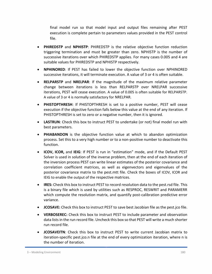
3 – Modeling Environment 180
final model run so that model input and output files remaining after PEST
execution is complete pertain to parameters values provided in the PEST control
file.
• PHIREDSTP and NPHISTP: PHIREDSTP is the relative objective function reduction triggering termination and must be greater than zero. NPHISTP is the number of successive iterations over which PHIREDSTP applies. For many cases 0.005 and 4 are suitable values for PHIREDSTP and NPHISTP respectively.
• NPHINORED: If PEST has failed to lower the objective function over NPHINORED successive iterations, it will terminate execution. A value of 3 or 4 is often suitable.
• RELPARSTP and NRELPAR: If the magnitude of the maximum relative parameter change between iterations is less than RELPARSTP over NRELPAR successive iterations, PEST will cease execution. A value of 0.005 is often suitable for RELPARSTP.
A value of 3 or 4 is normally satisfactory for NRELPAR.
• PHISTOPTHRESH: If PHISTOPTHRESH is set to a positive number, PEST will cease execution if the objective function falls below this value at the end of any iteration. If PHISTOPTHRESH is set to zero or a negative number, then it is ignored.
• LASTRUN: Check this box to instruct PEST to undertake (or not) final model run with best parameters.
• PHIABANDON is the objective function value at which to abandon optimization process. Set this to a very high number or to a non-positive number to deactivate this function.
• ICOV, ICOR, and IEIG: If PEST is run in “estimation” mode, and if the Default PEST Solver is used in solution of the inverse problem, then at the end of each iteration of the inversion process PEST can write linear estimates of the posterior covariance and correlation coefficient matrices, as well as eigenvectors and eigenvalues of the posterior covariance matrix to the pest.mtt file. Check the boxes of ICOV, ICOR and
IEIG to enable the output of the respective matrices.
• IRES: Check this box to instruct PEST to record resolution data to the pest.rsd file. This is a binary file which is used by utilities such as RESPROC, RESWRIT and PARAMERR which compute the resolution matrix, and quantify post-calibration predictive error variance.
• JCOSAVE: Check this box to instruct PEST to save best Jacobian file as the pest.jco file.
• VERBOSEREC: Check this box to instruct PEST to include parameter and observation data lists in the run record file. Uncheck this box so that PEST will write a much shorter run record file.
• JCOSAVEITN: Check this box to instruct PEST to write current Jacobian matrix to iteration-specific pest.jco.n file at the end of every optimization iteration, where n is the number of iteration.
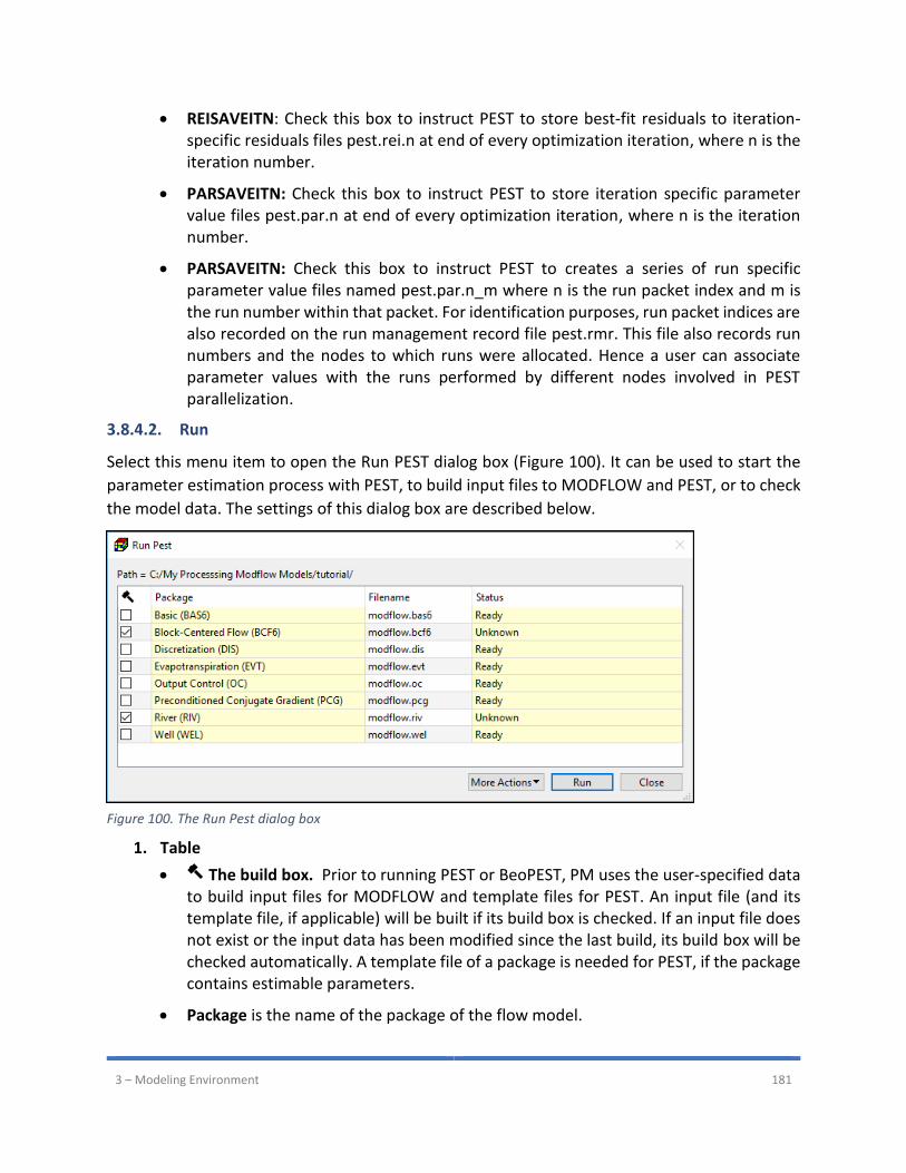
3 – Modeling Environment 181
• REISAVEITN: Check this box to instruct PEST to store best-fit residuals to iteration-specific residuals files pest.rei.n at end of every optimization iteration, where n is the iteration number.
• PARSAVEITN: Check this box to instruct PEST to store iteration specific parameter value files pest.par.n at end of every optimization iteration, where n is the iteration number.
• PARSAVEITN: Check this box to instruct PEST to creates a series of run specific parameter value files named pest.par.n_m where n is the run packet index and m is the run number within that packet. For identification purposes, run packet indices are also recorded on the run management record file pest.rmr. This file also records run numbers and the nodes to which runs were allocated. Hence a user can associate parameter values with the runs performed by different nodes involved in PEST parallelization.
3.8.4.2. Run
Select this menu item to open the Run PEST dialog box (Figure 100). It can be used to start the
parameter estimation process with PEST, to build input files to MODFLOW and PEST, or to check
the model data. The settings of this dialog box are described below.
1. Table
• The build box. Prior to running PEST or BeoPEST, PM uses the user-specified data to build input files for MODFLOW and template files for PEST. An input file (and its template file, if applicable) will be built if its build box is checked. If an input file does not exist or the input data has been modified since the last build, its build box will be checked automatically. A template file of a package is needed for PEST, if the package contains estimable parameters.
• Package is the name of the package of the flow model.
Figure 100. The Run Pest dialog box
3 – Modeling Environment 182
• Filename is the name of the input file to MODFLOW. The base filename of the corresponding template file to PEST is “pest”, instead of “modflow”.
• Status shows the status (such as Ready, Not Exist, etc.) of the input file.
2. More Actions
• Inspect Model Data: Select this to check the geometry of the model and the consistency of the model data. A list of items that are inspected by PM is given in Table 3. The inspection report will be saved in the modflow_inspection_log.txt file.
• Build Input Files: Select this to build the input files (and template files, if applicable) with the checked build boxes. The name file modflow.nam and input file modflow.lmt for LMT8 package will also be built. In addition, several batch files (*.bat) are also created for PEST and/or BeoPEST. Consult the build log files, modflow_build_log.txt and pest_build_log.txt for details. These files are in the model data folder.
• Rebuild All Input Files: Select this to rebuild all input files, except for existing input files that are marked as read-only.
3. Run: Click this button to build input files (and their template files) with the checked build boxes and the start the parameter estimation process. The following rules apply.
• If PEST Version (in the Preferences dialog box) is “Standard PEST”, the estimation process will be carried out by PEST. If PEST Version is “BeoPEST”, the estimation process will be carried out by BeoPEST.
• If LPF or BCF is selected as the internal flow package, the flow simulation will be carried out by MODFLOW-2005. If UPW is selected as the internal flow package, the flow simulation will be carried out by MODFLOW-NWT.
The PEST or BeoPEST run progress will be displayed in the PEST Output window. You may terminate the process at any time by clicking on the Terminate button.
3.8.4.3. Run PESTCHEK
Select this menu item to check for the correctness and consistency of the PEST control file built
by PM. PESTCHEK may provide additional advices beyond data checking. Running PESTCHEK is
normally not necessary, if the PEST or BeoPEST software that comes with PM are used.
3.8.4.4. View
The View menu allows you to display several output files of PEST. These files are briefly described
below. For detailed discussions, refer to Part I of the PEST Manual (Doherty, 2016).
Run Record File
As PEST executes, it writes a detailed record of the parameter estimation process to the run
record file pest.rec. if the parameters and/or observations are large in number this file can get
very long. In that case, you should uncheck VERBOSEREC box in the Control Data Tab of the PEST
Settings dialog box.
3 – Modeling Environment 183
Estimated Parameter Values
At the end optimization-iteration, PEST writes the best parameter set achieved so far (i.e., the
set for which the objective function is lowest) to the parameter file pest.par. The first line of the
file contains the values for the character variables PRECIS and DPOINT, which were used in the
PEST control file. Then follows a line for each parameter, each line containing a parameter name,
its current value and the values of the SCALE and OFFSET variables for that parameter. Using
values from intermediate parameter-estimation iterations, that are likely to be closer to the
optimal parameter values, often reduces execution time.
Residuals
On completion of parameter estimation process, PEST writes a “residuals file” tabulating
observation names, the groups to which observations belong, measured and modelled
observation values, differences between these two (i.e. residuals), measured and modelled
observation values multiplied by respective weights, weighted residuals, measurement standard
deviations and “natural weights”. This file can be readily imported into a spreadsheet for various
types of analysis and plotting. The name of the residuals file is pest.res.
Interim Residuals
At the beginning of each iteration PEST writes the interim residuals file pest.rei. It contains six
columns of data. The first two columns cite observation names and group names; then follow
observation values and their current model-generated counterparts. Current residuals and
weights follow that in subsequent columns.
Composite Parameter Sensitivities
Immediately after it calculates the Jacobian matrix, PEST writes composite parameter
sensitivities to the parameter sensitivity file pest.sen. The information contained in this file allows
you to track variations in the composite sensitivity of each parameter through the parameter
estimation process.
Composite Observation Sensitivities
The Observation Sensitivity file pest.seo contains all observation values and corresponding
model-calculated values, as well as composite sensitivities for all observations. The composite
sensitivity of an observation is a measure of the sensitivity of that observation to all parameters
involved in the parameter estimation process. A high value of composite observation sensitivity
normally indicates that an observation is particularly crucial to the inversion process.
SVD Output File
When SVD is activated, PEST writes the SVD output file pest.svd in addition to other output files.
The SVD output file can become very large and not all the information recorded in this file is

3 – Modeling Environment 184
always worth reading. However sometimes an inspection of singular values can assist in
understanding the degree to which an inverse problem is ill-posed.
Scatter Chart
To display the scatter chart based on the head data, select Scatter Chart > Head. To display the
scatter chart based on the drawdown data, select Scatter Chart > Drawdown. For details, see
Section 3.8.1.5.3.
Line Chart
To display the line chart based on the head data, select Line Chart > Head. To display the line
chart based on the drawdown data, select Line Chart > Drawdown. For details, see Section
3.8.1.5.4.

4 – Visualization and Postprocessing 185
Chapter 4. Visualization and Postprocessing
This chapter describes how to visualize and postprocess the input/output data of the active
model. The item of the active model on the TOC contains two major groups, namely Input Data
and Visualization. The former can be used to adjust visualization settings of the input data,
including model grid, flow packages, and observation points. The latter may include many types
of items, such as input parameter contours, simulation result contours, flow vectors, and
pathlines via MODPATH instances.
As mentioned in Chapter 1, each of these items on the TOC represents a map layer that contains
a visual representation of the item’s data. The available visualization settings of the active layer
are displayed in the Settings window. This chapter discusses these visualization settings.
4.1. Input Data
4.1.1. Model Grid
As shown in Figure 101, the display settings of the model grid are
organized in several groups based on the nature of the data.
These settings are described below. By right-clicking on the
Model Grid item and selecting Export to Shapefile, you can export
the shapefiles of the individual groups to a zip file.
1. General
• Display Layer: This is the layer number of the model grid. When multiple items are displayed on the Map Viewer, the items with smaller layer numbers are displayed on top of the items with larger layer numbers.
2. Model Bounding Box
• Visible: Check this box to turn on the display of the model bounding box encompassing all cells of the model.
• Opacity: The model box is opaque if the value of opacity is 100, translucent if the value is between 1 and 99, and transparent if the value is 0.
• Line Width is the line width (in pixels) that is used to draw the model box.
• Color: Use this dropdown box to select a color for the model box. Figure 101. The Settings window for
model grid
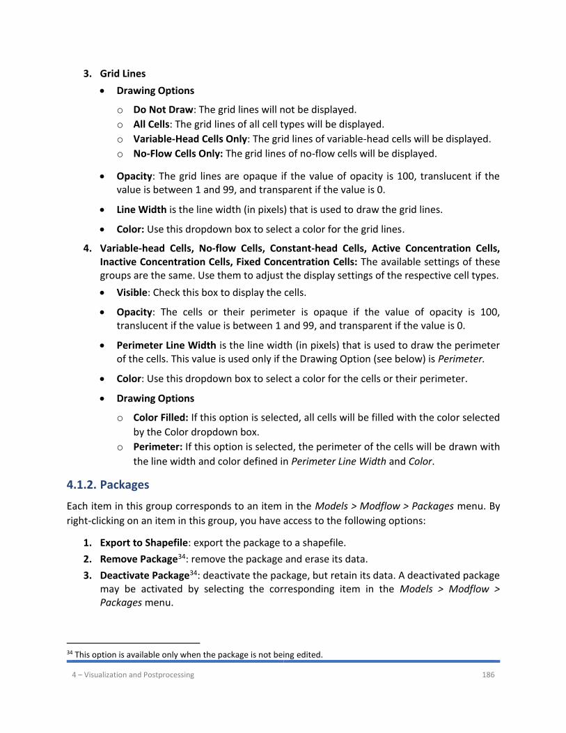
4 – Visualization and Postprocessing 186
3. Grid Lines
• Drawing Options
o Do Not Draw: The grid lines will not be displayed.
o All Cells: The grid lines of all cell types will be displayed.
o Variable-Head Cells Only: The grid lines of variable-head cells will be displayed.
o No-Flow Cells Only: The grid lines of no-flow cells will be displayed.
• Opacity: The grid lines are opaque if the value of opacity is 100, translucent if the value is between 1 and 99, and transparent if the value is 0.
• Line Width is the line width (in pixels) that is used to draw the grid lines.
• Color: Use this dropdown box to select a color for the grid lines.
4. Variable-head Cells, No-flow Cells, Constant-head Cells, Active Concentration Cells, Inactive Concentration Cells, Fixed Concentration Cells: The available settings of these groups are the same. Use them to adjust the display settings of the respective cell types.
• Visible: Check this box to display the cells.
• Opacity: The cells or their perimeter is opaque if the value of opacity is 100, translucent if the value is between 1 and 99, and transparent if the value is 0.
• Perimeter Line Width is the line width (in pixels) that is used to draw the perimeter of the cells. This value is used only if the Drawing Option (see below) is Perimeter.
• Color: Use this dropdown box to select a color for the cells or their perimeter.
• Drawing Options
o Color Filled: If this option is selected, all cells will be filled with the color selected
by the Color dropdown box.
o Perimeter: If this option is selected, the perimeter of the cells will be drawn with
the line width and color defined in Perimeter Line Width and Color.
4.1.2. Packages
Each item in this group corresponds to an item in the Models > Modflow > Packages menu. By
right-clicking on an item in this group, you have access to the following options:
1. Export to Shapefile: export the package to a shapefile.
2. Remove Package34: remove the package and erase its data.
3. Deactivate Package34: deactivate the package, but retain its data. A deactivated package may be activated by selecting the corresponding item in the Models > Modflow > Packages menu.
34 This option is available only when the package is not being edited.
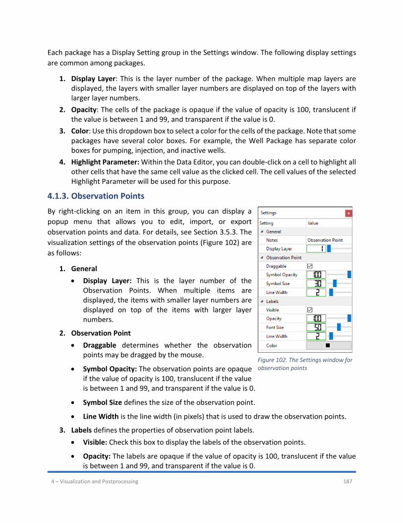
4 – Visualization and Postprocessing 187
Each package has a Display Setting group in the Settings window. The following display settings
are common among packages.
1. Display Layer: This is the layer number of the package. When multiple map layers are displayed, the layers with smaller layer numbers are displayed on top of the layers with larger layer numbers.
2. Opacity: The cells of the package is opaque if the value of opacity is 100, translucent if the value is between 1 and 99, and transparent if the value is 0.
3. Color: Use this dropdown box to select a color for the cells of the package. Note that some packages have several color boxes. For example, the Well Package has separate color boxes for pumping, injection, and inactive wells.
4. Highlight Parameter: Within the Data Editor, you can double-click on a cell to highlight all other cells that have the same cell value as the clicked cell. The cell values of the selected Highlight Parameter will be used for this purpose.
4.1.3. Observation Points
By right-clicking on an item in this group, you can display a
popup menu that allows you to edit, import, or export
observation points and data. For details, see Section 3.5.3. The
visualization settings of the observation points (Figure 102) are
as follows:
1. General
• Display Layer: This is the layer number of the Observation Points. When multiple items are displayed, the items with smaller layer numbers are displayed on top of the items with larger layer numbers.
2. Observation Point
• Draggable determines whether the observation points may be dragged by the mouse.
• Symbol Opacity: The observation points are opaque if the value of opacity is 100, translucent if the value is between 1 and 99, and transparent if the value is 0.
• Symbol Size defines the size of the observation point.
• Line Width is the line width (in pixels) that is used to draw the observation points.
3. Labels defines the properties of observation point labels.
• Visible: Check this box to display the labels of the observation points.
• Opacity: The labels are opaque if the value of opacity is 100, translucent if the value is between 1 and 99, and transparent if the value is 0.
Figure 102. The Settings window for observation points
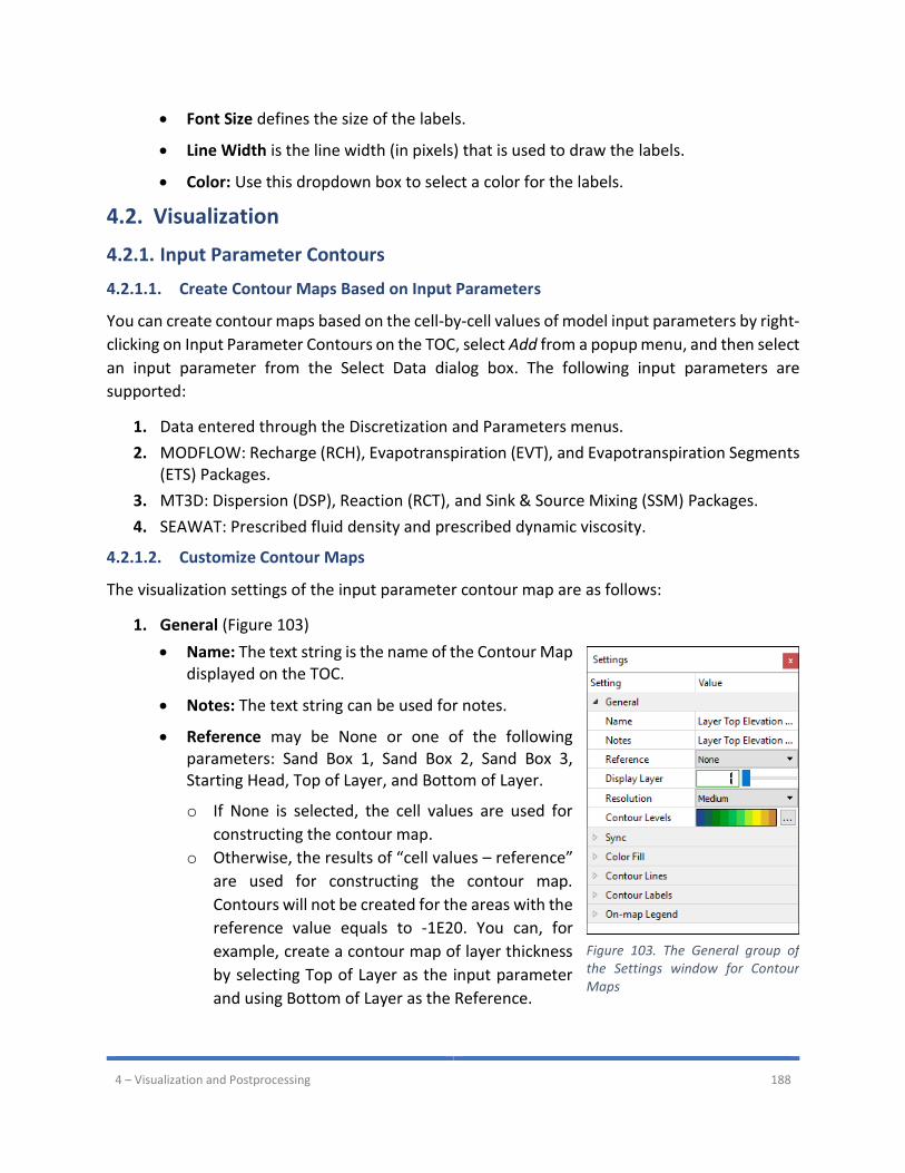
4 – Visualization and Postprocessing 188
• Font Size defines the size of the labels.
• Line Width is the line width (in pixels) that is used to draw the labels.
• Color: Use this dropdown box to select a color for the labels.
4.2. Visualization
4.2.1. Input Parameter Contours
4.2.1.1. Create Contour Maps Based on Input Parameters
You can create contour maps based on the cell-by-cell values of model input parameters by right-
clicking on Input Parameter Contours on the TOC, select Add from a popup menu, and then select
an input parameter from the Select Data dialog box. The following input parameters are
supported:
1. Data entered through the Discretization and Parameters menus.
2. MODFLOW: Recharge (RCH), Evapotranspiration (EVT), and Evapotranspiration Segments (ETS) Packages.
3. MT3D: Dispersion (DSP), Reaction (RCT), and Sink & Source Mixing (SSM) Packages.
4. SEAWAT: Prescribed fluid density and prescribed dynamic viscosity.
4.2.1.2. Customize Contour Maps
The visualization settings of the input parameter contour map are as follows:
1. General (Figure 103)
• Name: The text string is the name of the Contour Map displayed on the TOC.
• Notes: The text string can be used for notes.
• Reference may be None or one of the following parameters: Sand Box 1, Sand Box 2, Sand Box 3, Starting Head, Top of Layer, and Bottom of Layer.
o If None is selected, the cell values are used for
constructing the contour map.
o Otherwise, the results of “cell values – reference”
are used for constructing the contour map.
Contours will not be created for the areas with the
reference value equals to -1E20. You can, for
example, create a contour map of layer thickness
by selecting Top of Layer as the input parameter
and using Bottom of Layer as the Reference.
Figure 103. The General group of the Settings window for Contour Maps
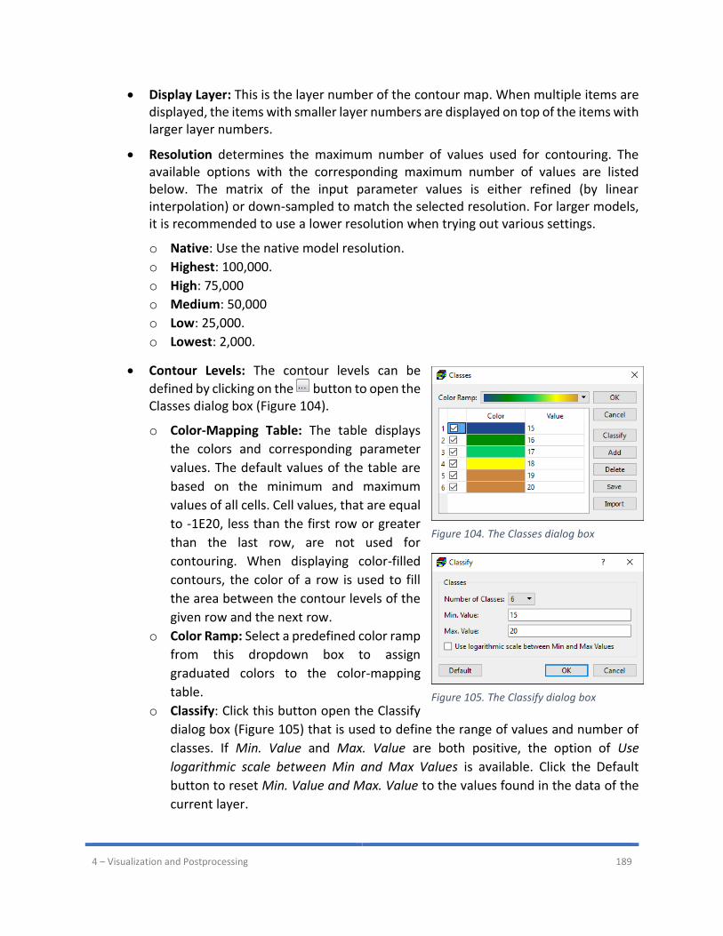
4 – Visualization and Postprocessing 189
• Display Layer: This is the layer number of the contour map. When multiple items are displayed, the items with smaller layer numbers are displayed on top of the items with larger layer numbers.
• Resolution determines the maximum number of values used for contouring. The available options with the corresponding maximum number of values are listed below. The matrix of the input parameter values is either refined (by linear interpolation) or down-sampled to match the selected resolution. For larger models, it is recommended to use a lower resolution when trying out various settings.
o Native: Use the native model resolution.
o Highest: 100,000.
o High: 75,000
o Medium: 50,000
o Low: 25,000.
o Lowest: 2,000.
• Contour Levels: The contour levels can be
defined by clicking on the button to open the Classes dialog box (Figure 104).
o Color-Mapping Table: The table displays
the colors and corresponding parameter
values. The default values of the table are
based on the minimum and maximum
values of all cells. Cell values, that are equal
to -1E20, less than the first row or greater
than the last row, are not used for
contouring. When displaying color-filled
contours, the color of a row is used to fill
the area between the contour levels of the
given row and the next row.
o Color Ramp: Select a predefined color ramp
from this dropdown box to assign
graduated colors to the color-mapping
table.
o Classify: Click this button open the Classify
dialog box (Figure 105) that is used to define the range of values and number of
classes. If Min. Value and Max. Value are both positive, the option of Use
logarithmic scale between Min and Max Values is available. Click the Default
button to reset Min. Value and Max. Value to the values found in the data of the
current layer.
Figure 104. The Classes dialog box
Figure 105. The Classify dialog box
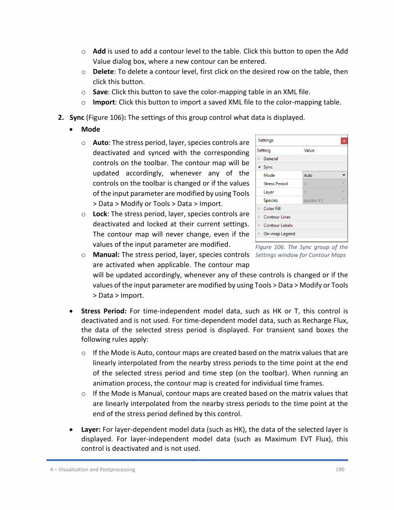
4 – Visualization and Postprocessing 190
o Add is used to add a contour level to the table. Click this button to open the Add
Value dialog box, where a new contour can be entered.
o Delete: To delete a contour level, first click on the desired row on the table, then
click this button.
o Save: Click this button to save the color-mapping table in an XML file.
o Import: Click this button to import a saved XML file to the color-mapping table.
2. Sync (Figure 106): The settings of this group control what data is displayed.
• Mode
o Auto: The stress period, layer, species controls are
deactivated and synced with the corresponding
controls on the toolbar. The contour map will be
updated accordingly, whenever any of the
controls on the toolbar is changed or if the values
of the input parameter are modified by using Tools
> Data > Modify or Tools > Data > Import.
o Lock: The stress period, layer, species controls are
deactivated and locked at their current settings.
The contour map will never change, even if the
values of the input parameter are modified.
o Manual: The stress period, layer, species controls
are activated when applicable. The contour map
will be updated accordingly, whenever any of these controls is changed or if the
values of the input parameter are modified by using Tools > Data > Modify or Tools
> Data > Import.
• Stress Period: For time-independent model data, such as HK or T, this control is deactivated and is not used. For time-dependent model data, such as Recharge Flux, the data of the selected stress period is displayed. For transient sand boxes the following rules apply:
o If the Mode is Auto, contour maps are created based on the matrix values that are
linearly interpolated from the nearby stress periods to the time point at the end
of the selected stress period and time step (on the toolbar). When running an
animation process, the contour map is created for individual time frames.
o If the Mode is Manual, contour maps are created based on the matrix values that
are linearly interpolated from the nearby stress periods to the time point at the
end of the stress period defined by this control.
• Layer: For layer-dependent model data (such as HK), the data of the selected layer is displayed. For layer-independent model data (such as Maximum EVT Flux), this control is deactivated and is not used.
Figure 106. The Sync group of the Settings window for Contour Maps
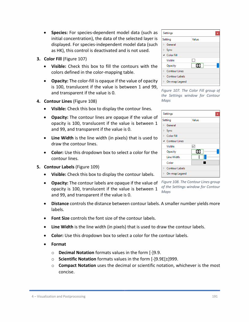
4 – Visualization and Postprocessing 191
• Species: For species-dependent model data (such as initial concentration), the data of the selected layer is displayed. For species-independent model data (such as HK), this control is deactivated and is not used.
3. Color Fill (Figure 107)
• Visible: Check this box to fill the contours with the colors defined in the color-mapping table.
• Opacity: The color-fill is opaque if the value of opacity is 100, translucent if the value is between 1 and 99, and transparent if the value is 0.
4. Contour Lines (Figure 108)
• Visible: Check this box to display the contour lines.
• Opacity: The contour lines are opaque if the value of opacity is 100, translucent if the value is between 1 and 99, and transparent if the value is 0.
• Line Width is the line width (in pixels) that is used to draw the contour lines.
• Color: Use this dropdown box to select a color for the contour lines.
5. Contour Labels (Figure 109)
• Visible: Check this box to display the contour labels.
• Opacity: The contour labels are opaque if the value of opacity is 100, translucent if the value is between 1 and 99, and transparent if the value is 0.
• Distance controls the distance between contour labels. A smaller number yields more labels.
• Font Size controls the font size of the contour labels.
• Line Width is the line width (in pixels) that is used to draw the contour labels.
• Color: Use this dropdown box to select a color for the contour labels.
• Format
o Decimal Notation formats values in the form [-]9.9.
o Scientific Notation formats values in the form [-]9.9E[±]999.
o Compact Notation uses the decimal or scientific notation, whichever is the most
concise.
Figure 107. The Color Fill group of the Settings window for Contour Maps
Figure 108. The Contour Lines group of the Settings window for Contour Maps
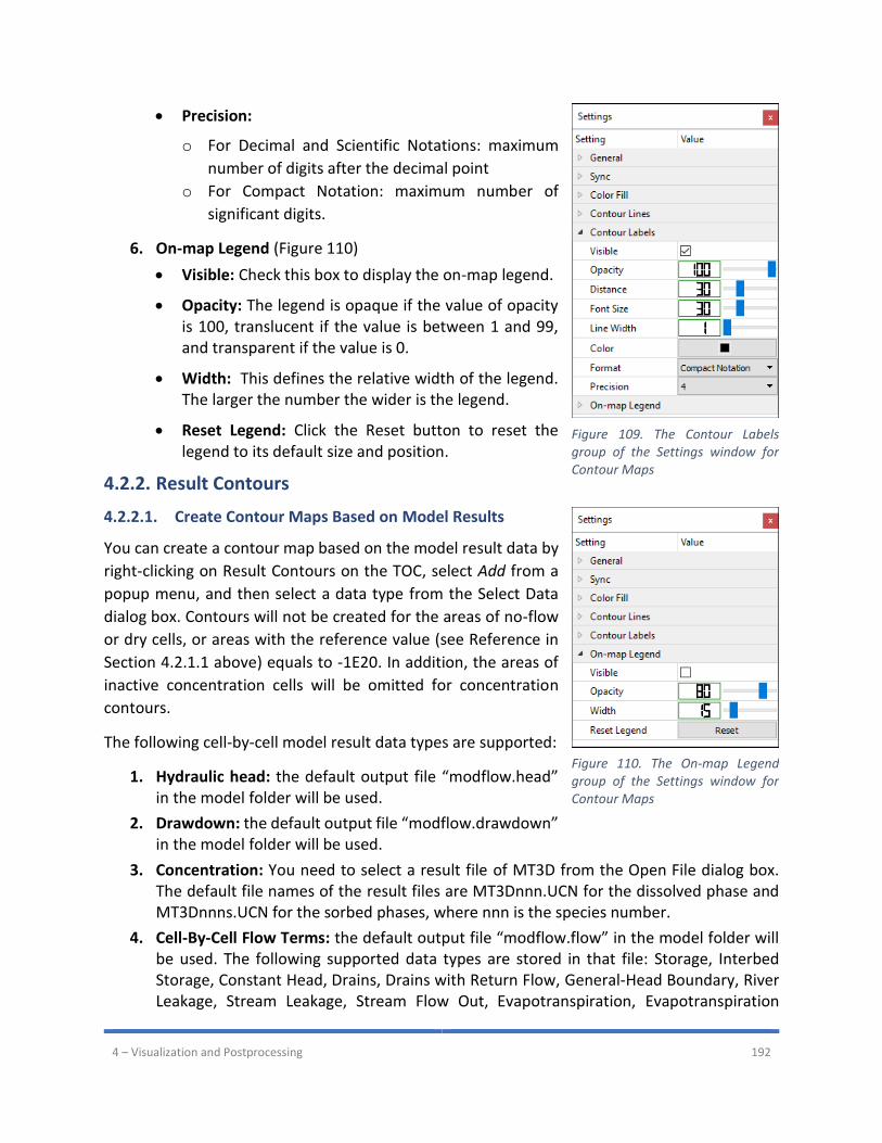
4 – Visualization and Postprocessing 192
• Precision:
o For Decimal and Scientific Notations: maximum
number of digits after the decimal point
o For Compact Notation: maximum number of
significant digits.
6. On-map Legend (Figure 110)
• Visible: Check this box to display the on-map legend.
• Opacity: The legend is opaque if the value of opacity is 100, translucent if the value is between 1 and 99, and transparent if the value is 0.
• Width: This defines the relative width of the legend. The larger the number the wider is the legend.
• Reset Legend: Click the Reset button to reset the legend to its default size and position.
4.2.2. Result Contours
4.2.2.1. Create Contour Maps Based on Model Results
You can create a contour map based on the model result data by
right-clicking on Result Contours on the TOC, select Add from a
popup menu, and then select a data type from the Select Data
dialog box. Contours will not be created for the areas of no-flow
or dry cells, or areas with the reference value (see Reference in
Section 4.2.1.1 above) equals to -1E20. In addition, the areas of
inactive concentration cells will be omitted for concentration
contours.
The following cell-by-cell model result data types are supported:
1. Hydraulic head: the default output file “modflow.head” in the model folder will be used.
2. Drawdown: the default output file “modflow.drawdown” in the model folder will be used.
3. Concentration: You need to select a result file of MT3D from the Open File dialog box. The default file names of the result files are MT3Dnnn.UCN for the dissolved phase and MT3Dnnns.UCN for the sorbed phases, where nnn is the species number.
4. Cell-By-Cell Flow Terms: the default output file “modflow.flow” in the model folder will be used. The following supported data types are stored in that file: Storage, Interbed Storage, Constant Head, Drains, Drains with Return Flow, General-Head Boundary, River Leakage, Stream Leakage, Stream Flow Out, Evapotranspiration, Evapotranspiration
Figure 109. The Contour Labels group of the Settings window for Contour Maps
Figure 110. The On-map Legend group of the Settings window for Contour Maps
4 – Visualization and Postprocessing 193
Segments, Recharge, Flow Right Face, Flow Front Face, Flow Lower Face, Horizontal Flux (flux at the cell center based on fluxes across the horizontal cell faces), Vertical flux (flux at the cell center based on fluxes across the top and bottom cell faces), Flux (flux at the cell center based on fluxes across all cell faces).
5. Interbed Storage Package: the default output file “modflow.interbed” in the model folder will be used. The following supported data types are stored in that file: Subsidence, Compaction, and Critical Head.
6. Seawater Intrusion 2 Package: The calculated interface elevation (Zeta surface elevation) are stored in the output file “modflow.swi2zeta” in the model folder. The following supported data types are stored in the “modflow.flow” file located in the model folder: Flow Right Face Correction, Flow Lower Face Correction, Flow Front Face Correction, and Constant Head Flow Correction. These correction terms are to be added to the corresponding cell-by-cell flow terms to yield the final flow results.
4.2.2.2. Customize Contour Maps
Most of the visualization settings of a result contour map are the same as those described in
Section 4.2.1.2. The following is a list containing the result-contour specific settings:
1. General
• Result File is the (read-only) name of the binary file that contains the cell-by-cell model result values. Refer to Section 5.2 for the output file names of the supported models.
2. Sync
• Mode
o Auto: The controls of the Sync group are deactivated and synced with the
corresponding controls on the toolbar. Whenever the model is run, or any of the
is changed, the contour map will be updated with the most recent model results.
o Lock: The stress period, layer, date/time, and output times controls are
deactivated and locked at their current settings. The contour map will never
change, even if the model results have changed.
o Manual: The stress period, layer, date/time, and output times controls are
activated when applicable. The contour map will be based on the model results of
the date/time defined by the Date/Time control.
• Date/Time is the date/time for which the model result is displayed. After editing of the date/time is finished35, the values for Stress Period and Time Step will update accordingly and the contour map will be updated with “model result – reference” at the given date/time.
35 Editing is finished when the Date/Time control loses focus or when enter is pressed.
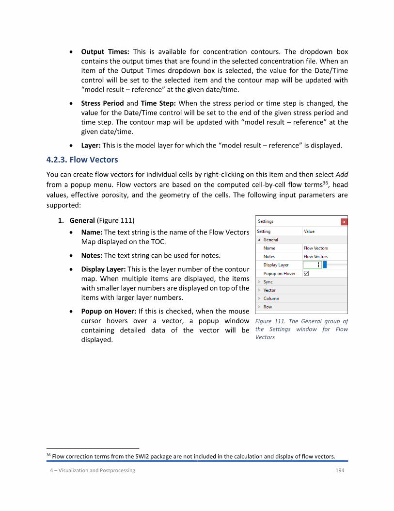
4 – Visualization and Postprocessing 194
• Output Times: This is available for concentration contours. The dropdown box contains the output times that are found in the selected concentration file. When an item of the Output Times dropdown box is selected, the value for the Date/Time control will be set to the selected item and the contour map will be updated with “model result – reference” at the given date/time.
• Stress Period and Time Step: When the stress period or time step is changed, the value for the Date/Time control will be set to the end of the given stress period and time step. The contour map will be updated with “model result – reference” at the given date/time.
• Layer: This is the model layer for which the “model result – reference” is displayed.
4.2.3. Flow Vectors
You can create flow vectors for individual cells by right-clicking on this item and then select Add
from a popup menu. Flow vectors are based on the computed cell-by-cell flow terms36, head
values, effective porosity, and the geometry of the cells. The following input parameters are
supported:
1. General (Figure 111)
• Name: The text string is the name of the Flow Vectors Map displayed on the TOC.
• Notes: The text string can be used for notes.
• Display Layer: This is the layer number of the contour map. When multiple items are displayed, the items with smaller layer numbers are displayed on top of the items with larger layer numbers.
• Popup on Hover: If this is checked, when the mouse cursor hovers over a vector, a popup window containing detailed data of the vector will be displayed.
36 Flow correction terms from the SWI2 package are not included in the calculation and display of flow vectors.
Figure 111. The General group of the Settings window for Flow Vectors

4 – Visualization and Postprocessing 195
2. Sync (Figure 112)
• Mode
o Auto: The stress period, time step and layer
controls are deactivated and synced with the
corresponding controls on the toolbar. Whenever
the model is run or any of the controls is changed,
the contour map will be updated based on the
most recent model results.
o Lock: The stress period, layer, species controls are
deactivated and locked at their current settings.
The contour map will never change, even if the
model results have changed.
o Manual: The stress period, layer, species controls
are activated when applicable. The contour map
will be created based on the model results of the
specified stress period, time step, and species when applicable.
• Date/Time is the date/time for which the model result is displayed. After editing of the date/time is finished, the values for Stress Period and Time Step will update accordingly and the flow vectors will be updated with the model result at the given date/time.
• Stress Period and Time Step: When the stress period or time step is changed, the value for the Date/Time control will be set to the end of the given stress period and time step. The flow vectors will be updated with model result at the given date/time.
• Layer: This is the model layer for which the flow vectors are displayed.
3. Vector (Figure 113)
Figure 112. The Sync group of the Settings window for Flow Vectors
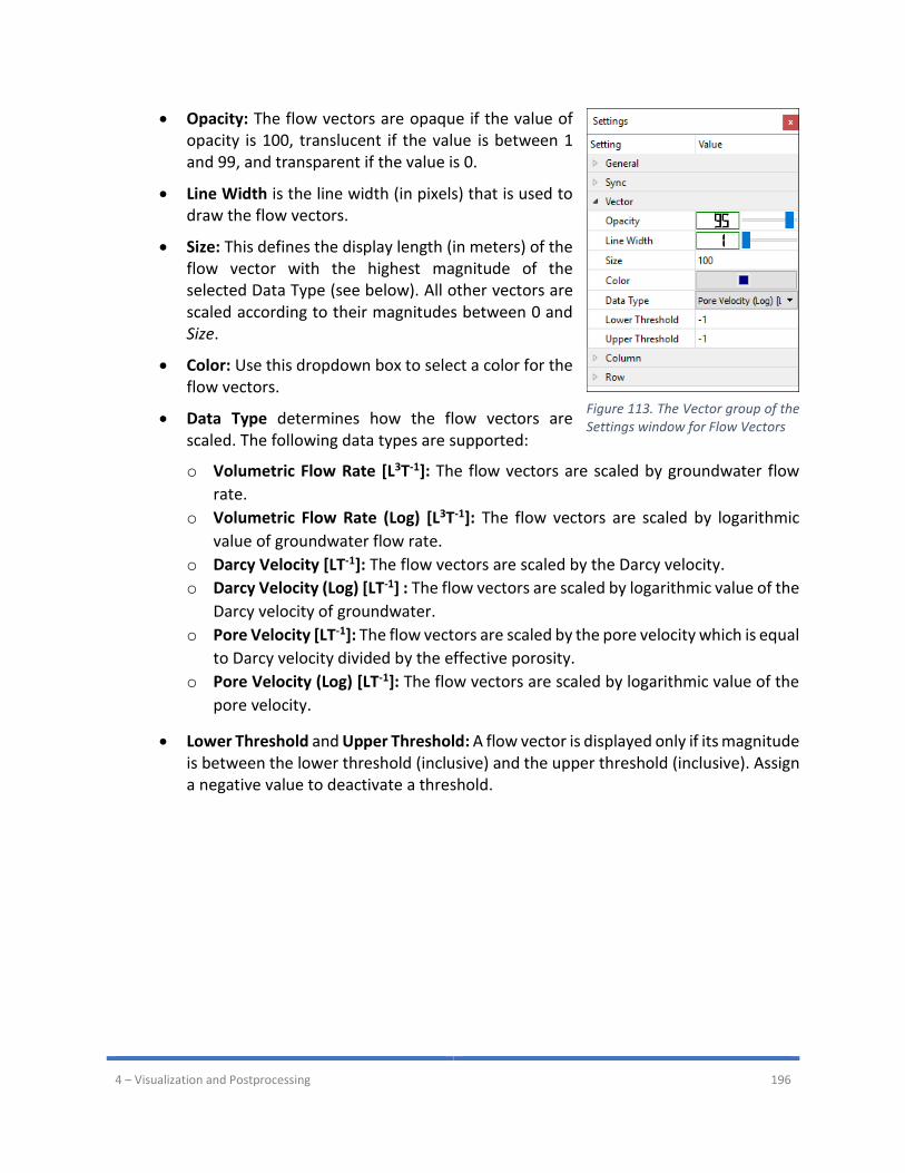
4 – Visualization and Postprocessing 196
• Opacity: The flow vectors are opaque if the value of opacity is 100, translucent if the value is between 1 and 99, and transparent if the value is 0.
• Line Width is the line width (in pixels) that is used to draw the flow vectors.
• Size: This defines the display length (in meters) of the flow vector with the highest magnitude of the selected Data Type (see below). All other vectors are scaled according to their magnitudes between 0 and Size.
• Color: Use this dropdown box to select a color for the flow vectors.
• Data Type determines how the flow vectors are scaled. The following data types are supported:
o Volumetric Flow Rate [L3T-1]: The flow vectors are scaled by groundwater flow
rate.
o Volumetric Flow Rate (Log) [L3T-1]: The flow vectors are scaled by logarithmic
value of groundwater flow rate.
o Darcy Velocity [LT-1]: The flow vectors are scaled by the Darcy velocity.
o Darcy Velocity (Log) [LT-1] : The flow vectors are scaled by logarithmic value of the
Darcy velocity of groundwater.
o Pore Velocity [LT-1]: The flow vectors are scaled by the pore velocity which is equal
to Darcy velocity divided by the effective porosity.
o Pore Velocity (Log) [LT-1]: The flow vectors are scaled by logarithmic value of the
pore velocity.
• Lower Threshold and Upper Threshold: A flow vector is displayed only if its magnitude is between the lower threshold (inclusive) and the upper threshold (inclusive). Assign a negative value to deactivate a threshold.
Figure 113. The Vector group of the Settings window for Flow Vectors
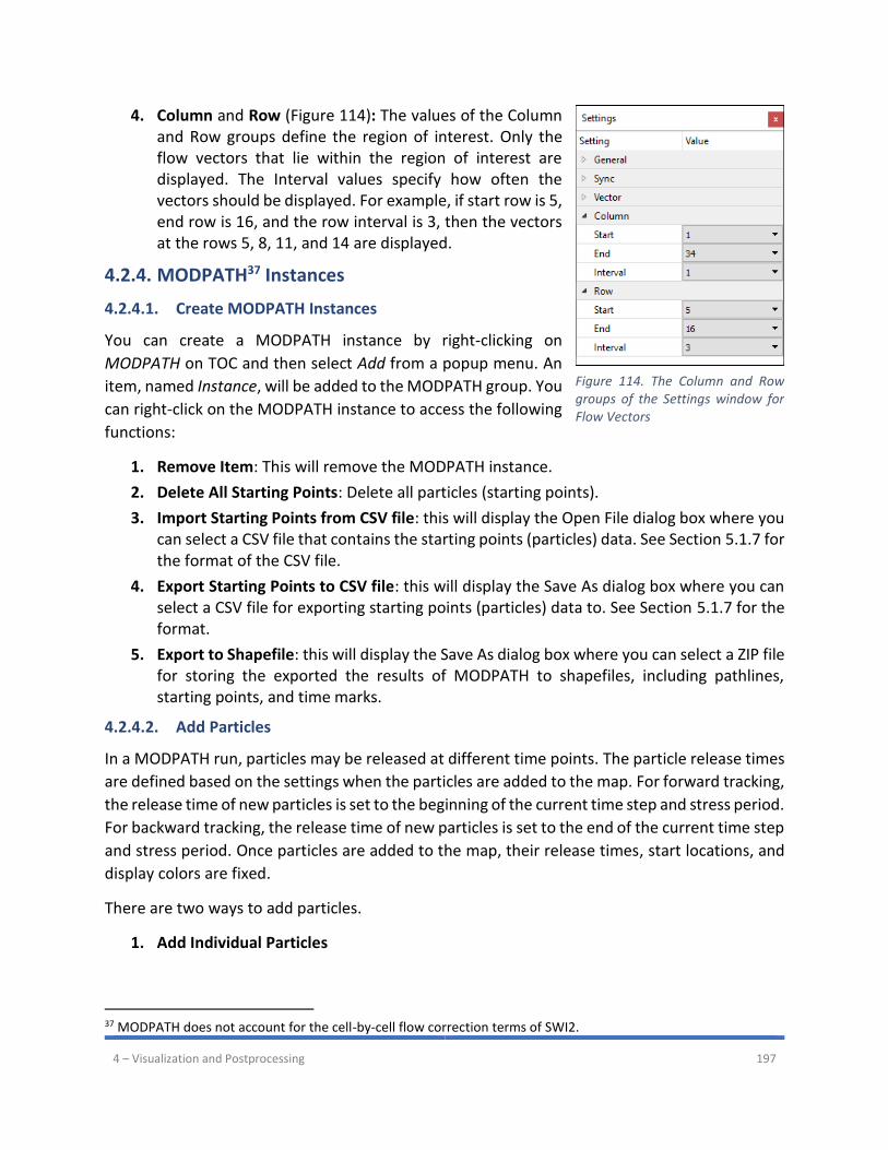
4 – Visualization and Postprocessing 197
4. Column and Row (Figure 114): The values of the Column and Row groups define the region of interest. Only the flow vectors that lie within the region of interest are displayed. The Interval values specify how often the vectors should be displayed. For example, if start row is 5, end row is 16, and the row interval is 3, then the vectors at the rows 5, 8, 11, and 14 are displayed.
4.2.4. MODPATH37 Instances
4.2.4.1. Create MODPATH Instances
You can create a MODPATH instance by right-clicking on
MODPATH on TOC and then select Add from a popup menu. An
item, named Instance, will be added to the MODPATH group. You
can right-click on the MODPATH instance to access the following
functions:
1. Remove Item: This will remove the MODPATH instance.
2. Delete All Starting Points: Delete all particles (starting points).
3. Import Starting Points from CSV file: this will display the Open File dialog box where you can select a CSV file that contains the starting points (particles) data. See Section 5.1.7 for the format of the CSV file.
4. Export Starting Points to CSV file: this will display the Save As dialog box where you can select a CSV file for exporting starting points (particles) data to. See Section 5.1.7 for the format.
5. Export to Shapefile: this will display the Save As dialog box where you can select a ZIP file for storing the exported the results of MODPATH to shapefiles, including pathlines, starting points, and time marks.
4.2.4.2. Add Particles
In a MODPATH run, particles may be released at different time points. The particle release times
are defined based on the settings when the particles are added to the map. For forward tracking,
the release time of new particles is set to the beginning of the current time step and stress period.
For backward tracking, the release time of new particles is set to the end of the current time step
and stress period. Once particles are added to the map, their release times, start locations, and
display colors are fixed.
There are two ways to add particles.
1. Add Individual Particles
37 MODPATH does not account for the cell-by-cell flow correction terms of SWI2.
Figure 114. The Column and Row groups of the Settings window for Flow Vectors
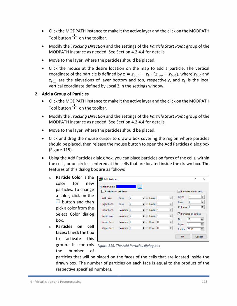
4 – Visualization and Postprocessing 198
• Click the MODPATH instance to make it the active layer and the click on the MODPATH
Tool button on the toolbar.
• Modify the Tracking Direction and the settings of the Particle Start Point group of the MODPATH instance as needed. See Section 4.2.4.4 for details.
• Move to the layer, where the particles should be placed.
• Click the mouse at the desire location on the map to add a particle. The vertical coordinate of the particle is defined by 𝑧 = 𝑧𝑏𝑜𝑡 + 𝑧𝐿 ⋅ (𝑧𝑡𝑜𝑝 − 𝑧𝑏𝑜𝑡), where 𝑧𝑏𝑜𝑡 and
𝑧𝑡𝑜𝑝 are the elevations of layer bottom and top, respectively, and 𝑧𝐿 is the local
vertical coordinate defined by Local Z in the settings window.
2. Add a Group of Particles
• Click the MODPATH instance to make it the active layer and the click on the MODPATH
Tool button on the toolbar.
• Modify the Tracking Direction and the settings of the Particle Start Point group of the MODPATH instance as needed. See Section 4.2.4.4 for details.
• Move to the layer, where the particles should be placed.
• Click and drag the mouse cursor to draw a box covering the region where particles should be placed, then release the mouse button to open the Add Particles dialog box (Figure 115).
• Using the Add Particles dialog box, you can place particles on faces of the cells, within the cells, or on circles centered at the cells that are located inside the drawn box. The features of this dialog box are as follows
o Particle Color is the
color for new
particles. To change
a color, click on the
button and then
pick a color from the
Select Color dialog
box.
o Particles on cell
faces: Check the box
to activate this
group. It controls
the number of
particles that will be placed on the faces of the cells that are located inside the
drawn box. The number of particles on each face is equal to the product of the
respective specified numbers.
Figure 115. The Add Particles dialog box
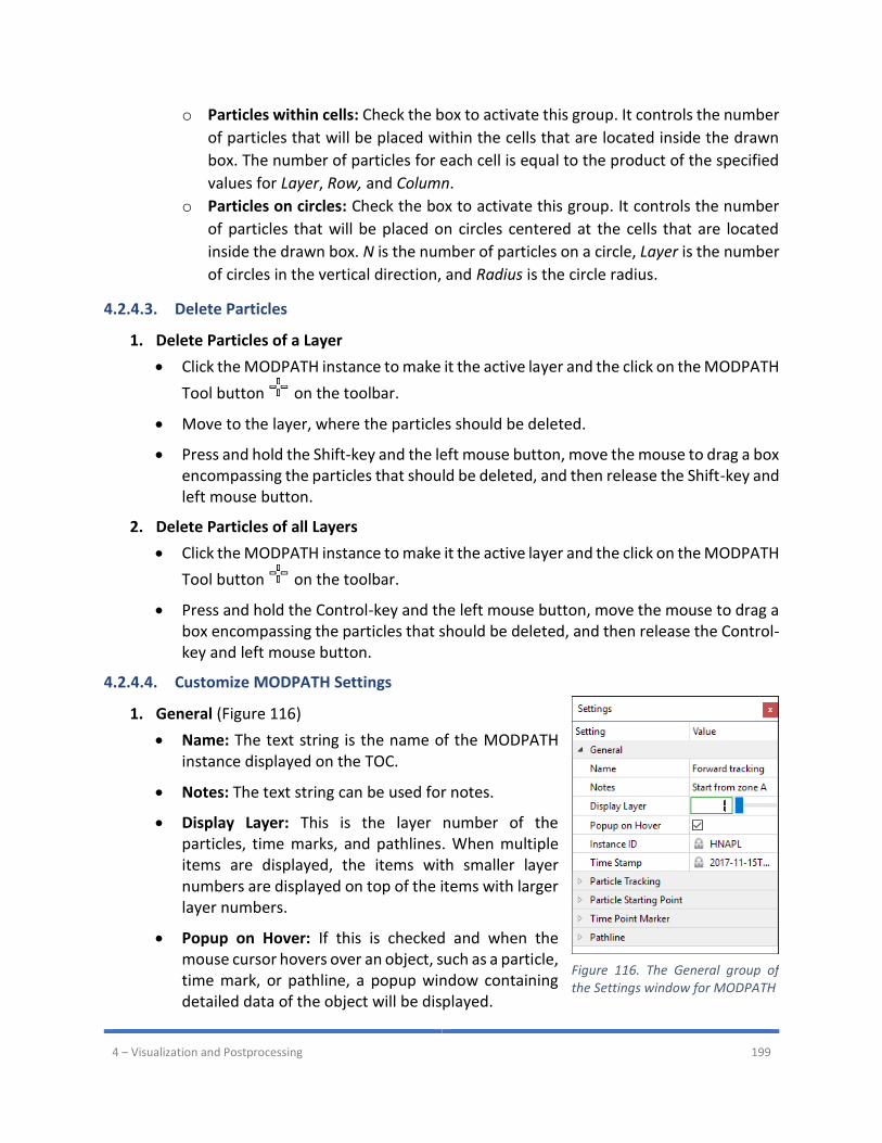
4 – Visualization and Postprocessing 199
o Particles within cells: Check the box to activate this group. It controls the number
of particles that will be placed within the cells that are located inside the drawn
box. The number of particles for each cell is equal to the product of the specified
values for Layer, Row, and Column.
o Particles on circles: Check the box to activate this group. It controls the number
of particles that will be placed on circles centered at the cells that are located
inside the drawn box. N is the number of particles on a circle, Layer is the number
of circles in the vertical direction, and Radius is the circle radius.
4.2.4.3. Delete Particles
1. Delete Particles of a Layer
• Click the MODPATH instance to make it the active layer and the click on the MODPATH
Tool button on the toolbar.
• Move to the layer, where the particles should be deleted.
• Press and hold the Shift-key and the left mouse button, move the mouse to drag a box encompassing the particles that should be deleted, and then release the Shift-key and left mouse button.
2. Delete Particles of all Layers
• Click the MODPATH instance to make it the active layer and the click on the MODPATH
Tool button on the toolbar.
• Press and hold the Control-key and the left mouse button, move the mouse to drag a box encompassing the particles that should be deleted, and then release the Control-key and left mouse button.
4.2.4.4. Customize MODPATH Settings
1. General (Figure 116)
• Name: The text string is the name of the MODPATH instance displayed on the TOC.
• Notes: The text string can be used for notes.
• Display Layer: This is the layer number of the particles, time marks, and pathlines. When multiple items are displayed, the items with smaller layer numbers are displayed on top of the items with larger layer numbers.
• Popup on Hover: If this is checked and when the mouse cursor hovers over an object, such as a particle, time mark, or pathline, a popup window containing detailed data of the object will be displayed.
Figure 116. The General group of the Settings window for MODPATH
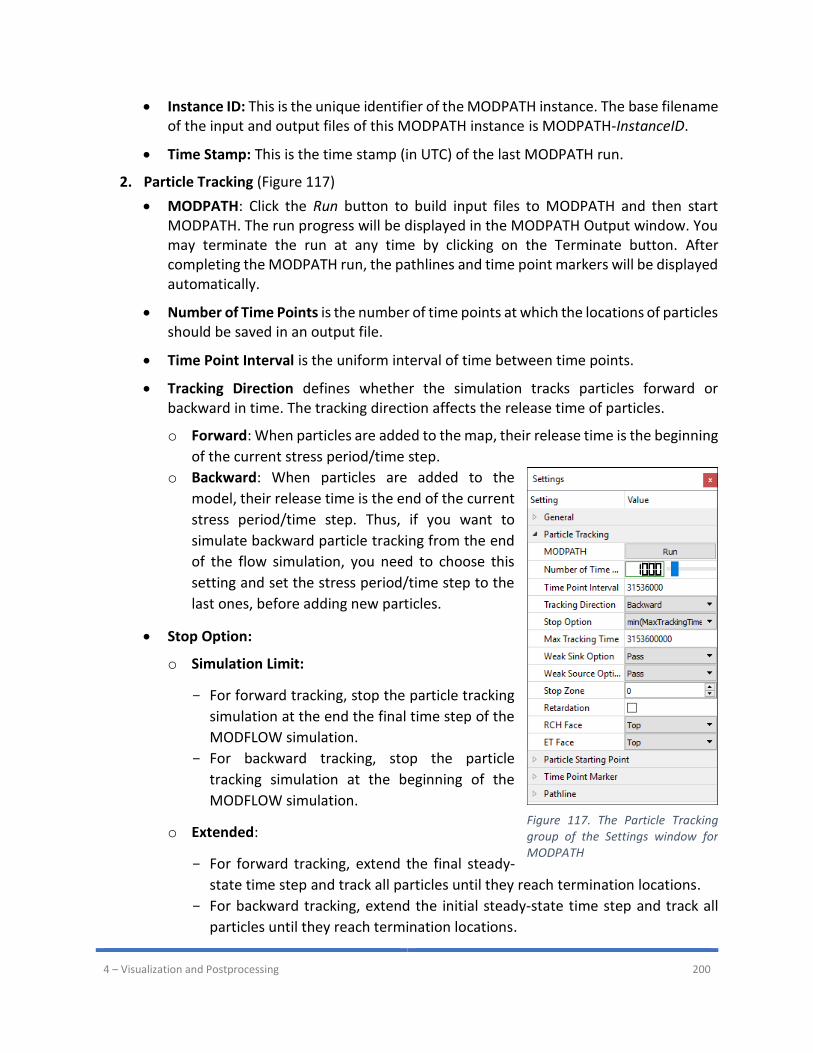
4 – Visualization and Postprocessing 200
• Instance ID: This is the unique identifier of the MODPATH instance. The base filename of the input and output files of this MODPATH instance is MODPATH-InstanceID.
• Time Stamp: This is the time stamp (in UTC) of the last MODPATH run.
2. Particle Tracking (Figure 117)
• MODPATH: Click the Run button to build input files to MODPATH and then start MODPATH. The run progress will be displayed in the MODPATH Output window. You may terminate the run at any time by clicking on the Terminate button. After completing the MODPATH run, the pathlines and time point markers will be displayed automatically.
• Number of Time Points is the number of time points at which the locations of particles should be saved in an output file.
• Time Point Interval is the uniform interval of time between time points.
• Tracking Direction defines whether the simulation tracks particles forward or backward in time. The tracking direction affects the release time of particles.
o Forward: When particles are added to the map, their release time is the beginning
of the current stress period/time step.
o Backward: When particles are added to the
model, their release time is the end of the current
stress period/time step. Thus, if you want to
simulate backward particle tracking from the end
of the flow simulation, you need to choose this
setting and set the stress period/time step to the
last ones, before adding new particles.
• Stop Option:
o Simulation Limit:
For forward tracking, stop the particle tracking
simulation at the end the final time step of the
MODFLOW simulation.
For backward tracking, stop the particle
tracking simulation at the beginning of the
MODFLOW simulation.
o Extended:
For forward tracking, extend the final steady-
state time step and track all particles until they reach termination locations.
For backward tracking, extend the initial steady-state time step and track all
particles until they reach termination locations.
Figure 117. The Particle Tracking group of the Settings window for MODPATH
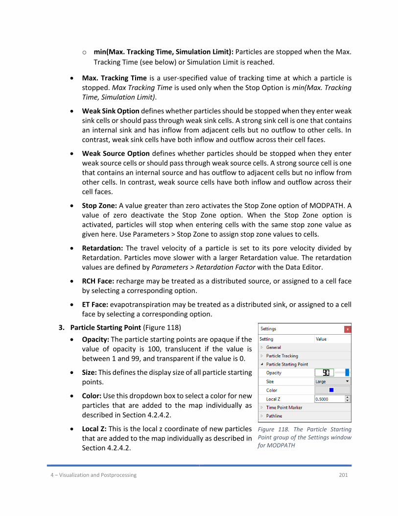
4 – Visualization and Postprocessing 201
o min(Max. Tracking Time, Simulation Limit): Particles are stopped when the Max.
Tracking Time (see below) or Simulation Limit is reached.
• Max. Tracking Time is a user-specified value of tracking time at which a particle is stopped. Max Tracking Time is used only when the Stop Option is min(Max. Tracking Time, Simulation Limit).
• Weak Sink Option defines whether particles should be stopped when they enter weak sink cells or should pass through weak sink cells. A strong sink cell is one that contains an internal sink and has inflow from adjacent cells but no outflow to other cells. In contrast, weak sink cells have both inflow and outflow across their cell faces.
• Weak Source Option defines whether particles should be stopped when they enter weak source cells or should pass through weak source cells. A strong source cell is one that contains an internal source and has outflow to adjacent cells but no inflow from other cells. In contrast, weak source cells have both inflow and outflow across their cell faces.
• Stop Zone: A value greater than zero activates the Stop Zone option of MODPATH. A value of zero deactivate the Stop Zone option. When the Stop Zone option is activated, particles will stop when entering cells with the same stop zone value as given here. Use Parameters > Stop Zone to assign stop zone values to cells.
• Retardation: The travel velocity of a particle is set to its pore velocity divided by Retardation. Particles move slower with a larger Retardation value. The retardation values are defined by Parameters > Retardation Factor with the Data Editor.
• RCH Face: recharge may be treated as a distributed source, or assigned to a cell face by selecting a corresponding option.
• ET Face: evapotranspiration may be treated as a distributed sink, or assigned to a cell face by selecting a corresponding option.
3. Particle Starting Point (Figure 118)
• Opacity: The particle starting points are opaque if the value of opacity is 100, translucent if the value is between 1 and 99, and transparent if the value is 0.
• Size: This defines the display size of all particle starting points.
• Color: Use this dropdown box to select a color for new particles that are added to the map individually as described in Section 4.2.4.2.
• Local Z: This is the local z coordinate of new particles that are added to the map individually as described in Section 4.2.4.2.
Figure 118. The Particle Starting Point group of the Settings window for MODPATH
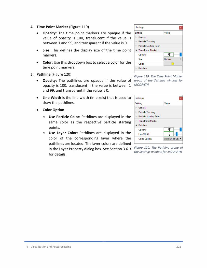
4 – Visualization and Postprocessing 202
4. Time Point Marker (Figure 119)
• Opacity: The time point markers are opaque if the value of opacity is 100, translucent if the value is between 1 and 99, and transparent if the value is 0.
• Size: This defines the display size of the time point markers.
• Color: Use this dropdown box to select a color for the time point markers.
5. Pathline (Figure 120)
• Opacity: The pathlines are opaque if the value of opacity is 100, translucent if the value is between 1 and 99, and transparent if the value is 0.
• Line Width is the line width (in pixels) that is used to draw the pathlines.
• Color Option
o Use Particle Color: Pathlines are displayed in the
same color as the respective particle starting
points.
o Use Layer Color: Pathlines are displayed in the
color of the corresponding layer where the
pathlines are located. The layer colors are defined
in the Layer Property dialog box. See Section 3.6.3
for details.
Figure 119. The Time Point Marker group of the Settings window for MODPATH
Figure 120. The Pathline group of the Settings window for MODPATH
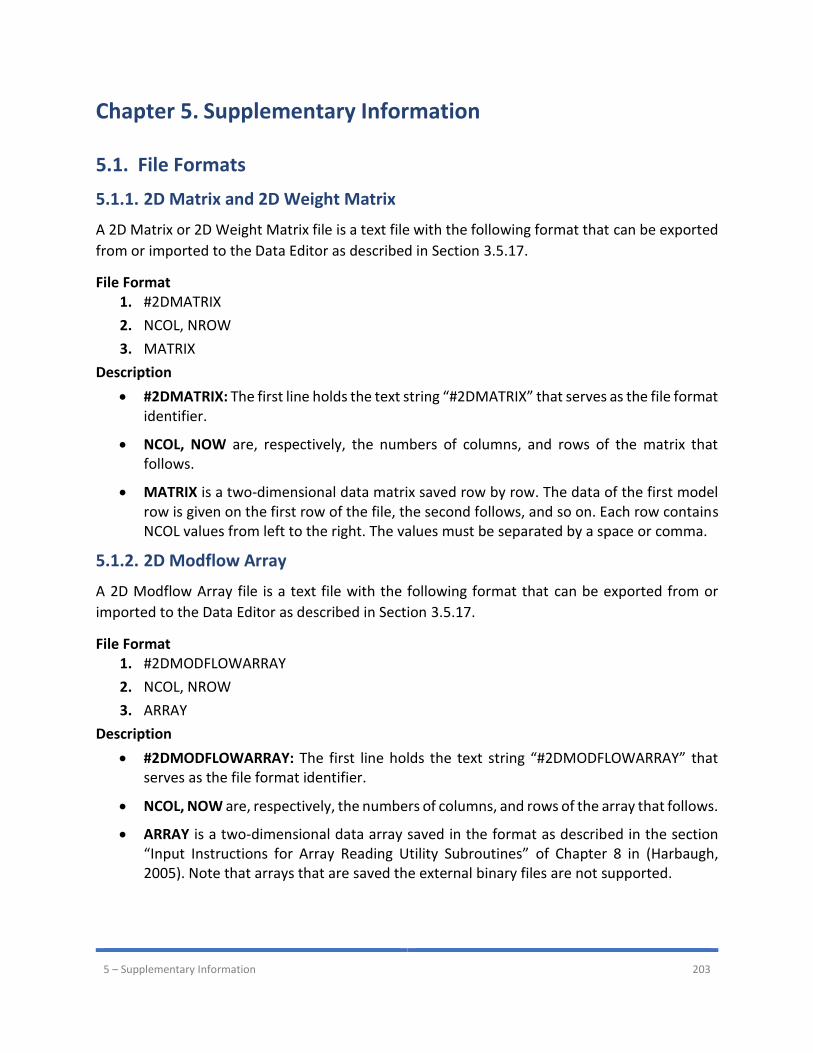
5 – Supplementary Information 203
Chapter 5. Supplementary Information
5.1. File Formats
5.1.1. 2D Matrix and 2D Weight Matrix
A 2D Matrix or 2D Weight Matrix file is a text file with the following format that can be exported
from or imported to the Data Editor as described in Section 3.5.17.
File Format 1. #2DMATRIX
2. NCOL, NROW
3. MATRIX
Description
• #2DMATRIX: The first line holds the text string “#2DMATRIX” that serves as the file format identifier.
• NCOL, NOW are, respectively, the numbers of columns, and rows of the matrix that follows.
• MATRIX is a two-dimensional data matrix saved row by row. The data of the first model row is given on the first row of the file, the second follows, and so on. Each row contains NCOL values from left to the right. The values must be separated by a space or comma.
5.1.2. 2D Modflow Array
A 2D Modflow Array file is a text file with the following format that can be exported from or
imported to the Data Editor as described in Section 3.5.17.
File Format 1. #2DMODFLOWARRAY
2. NCOL, NROW
3. ARRAY
Description
• #2DMODFLOWARRAY: The first line holds the text string “#2DMODFLOWARRAY” that serves as the file format identifier.
• NCOL, NOW are, respectively, the numbers of columns, and rows of the array that follows.
• ARRAY is a two-dimensional data array saved in the format as described in the section “Input Instructions for Array Reading Utility Subroutines” of Chapter 8 in (Harbaugh, 2005). Note that arrays that are saved the external binary files are not supported.
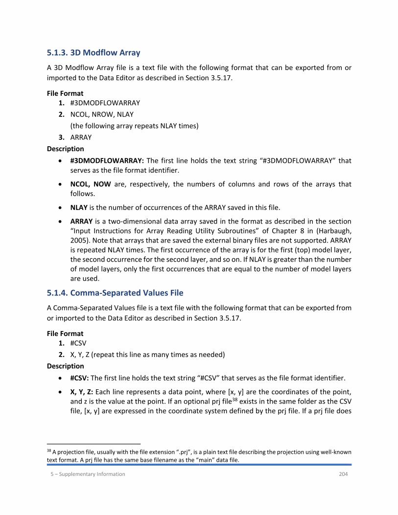
5 – Supplementary Information 204
5.1.3. 3D Modflow Array
A 3D Modflow Array file is a text file with the following format that can be exported from or
imported to the Data Editor as described in Section 3.5.17.
File Format 1. #3DMODFLOWARRAY
2. NCOL, NROW, NLAY
(the following array repeats NLAY times)
3. ARRAY
Description
• #3DMODFLOWARRAY: The first line holds the text string “#3DMODFLOWARRAY” that serves as the file format identifier.
• NCOL, NOW are, respectively, the numbers of columns and rows of the arrays that follows.
• NLAY is the number of occurrences of the ARRAY saved in this file.
• ARRAY is a two-dimensional data array saved in the format as described in the section “Input Instructions for Array Reading Utility Subroutines” of Chapter 8 in (Harbaugh, 2005). Note that arrays that are saved the external binary files are not supported. ARRAY is repeated NLAY times. The first occurrence of the array is for the first (top) model layer, the second occurrence for the second layer, and so on. If NLAY is greater than the number of model layers, only the first occurrences that are equal to the number of model layers are used.
5.1.4. Comma-Separated Values File
A Comma-Separated Values file is a text file with the following format that can be exported from
or imported to the Data Editor as described in Section 3.5.17.
File Format 1. #CSV
2. X, Y, Z (repeat this line as many times as needed)
Description
• #CSV: The first line holds the text string “#CSV” that serves as the file format identifier.
• X, Y, Z: Each line represents a data point, where [x, y] are the coordinates of the point, and z is the value at the point. If an optional prj file38 exists in the same folder as the CSV file, [x, y] are expressed in the coordinate system defined by the prj file. If a prj file does
38 A projection file, usually with the file extension “.prj”, is a plain text file describing the projection using well-known text format. A prj file has the same base filename as the “main” data file.
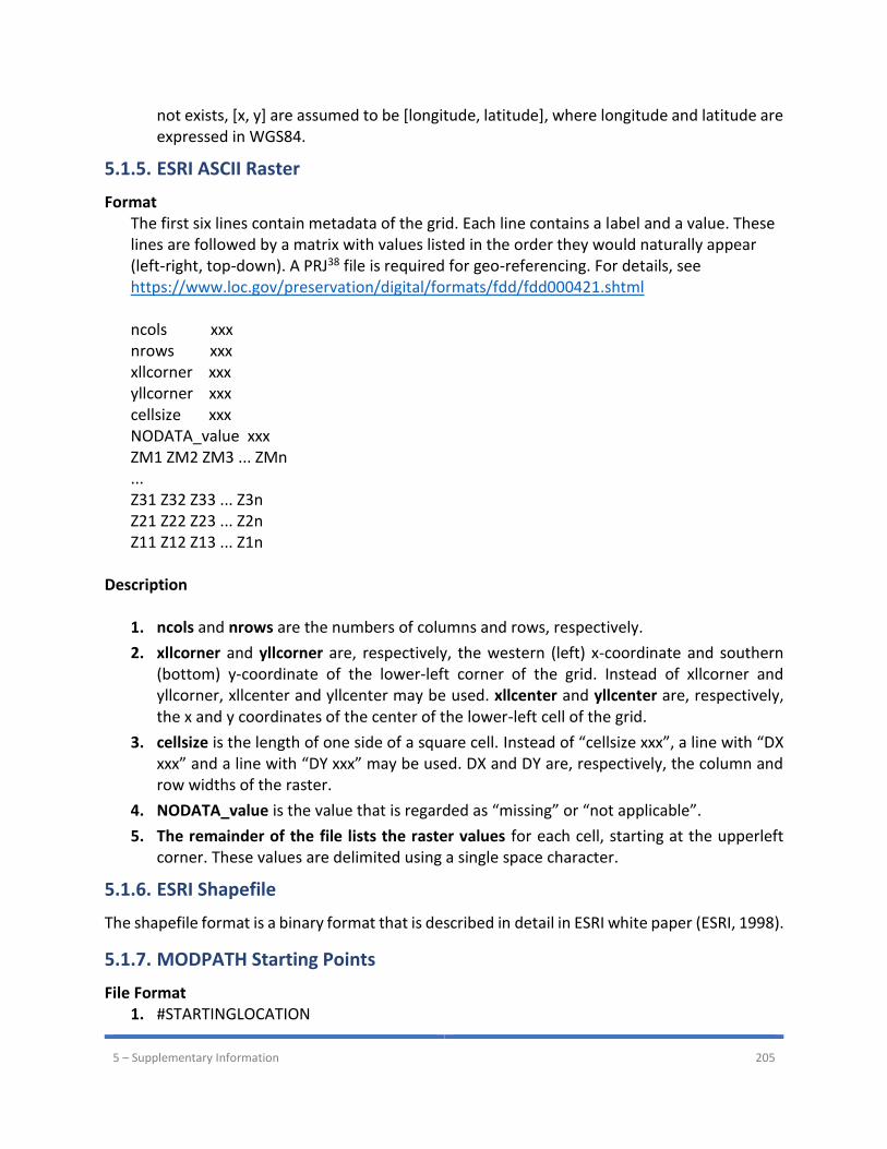
5 – Supplementary Information 205
not exists, [x, y] are assumed to be [longitude, latitude], where longitude and latitude are expressed in WGS84.
5.1.5. ESRI ASCII Raster
Format The first six lines contain metadata of the grid. Each line contains a label and a value. These lines are followed by a matrix with values listed in the order they would naturally appear (left-right, top-down). A PRJ38 file is required for geo-referencing. For details, see https://www.loc.gov/preservation/digital/formats/fdd/fdd000421.shtml ncols xxx nrows xxx xllcorner xxx yllcorner xxx cellsize xxx NODATA_value xxx ZM1 ZM2 ZM3 ... ZMn ... Z31 Z32 Z33 ... Z3n Z21 Z22 Z23 ... Z2n Z11 Z12 Z13 ... Z1n
Description
1. ncols and nrows are the numbers of columns and rows, respectively.
2. xllcorner and yllcorner are, respectively, the western (left) x-coordinate and southern (bottom) y-coordinate of the lower-left corner of the grid. Instead of xllcorner and yllcorner, xllcenter and yllcenter may be used. xllcenter and yllcenter are, respectively, the x and y coordinates of the center of the lower-left cell of the grid.
3. cellsize is the length of one side of a square cell. Instead of “cellsize xxx”, a line with “DX xxx” and a line with “DY xxx” may be used. DX and DY are, respectively, the column and row widths of the raster.
4. NODATA_value is the value that is regarded as “missing” or “not applicable”.
5. The remainder of the file lists the raster values for each cell, starting at the upperleft corner. These values are delimited using a single space character.
5.1.6. ESRI Shapefile
The shapefile format is a binary format that is described in detail in ESRI white paper (ESRI, 1998).
5.1.7. MODPATH Starting Points
File Format 1. #STARTINGLOCATION

5 – Supplementary Information 206
2. Version
3. N
(the following record repeats N times)
4. Layer, row, column, localX, localY, localZ, elapsedTime
Description
• #STARTINGLOCATION: The first line holds the text string “#STARTINGLOCATION” that serves as the file format identifier.
• Version is reserved for file version. The default value of 1.0 should be used.
• N is the number of starting points (particles) saved in this file.
• Layer, row, column, localX, localY, localZ, elapsedTime: each line represents a starting point.
o Layer, row, and column are the cell where the particle is located.
o localX, localY, and localZ are the local coordinates of the particle within the cell.
The value of local coordinates range between 0 and 1.
o elapsedTime is the release time of the particle expressed as the elapsed time (in
the model time unit) since the start of the flow simulation.
5.1.8. Georeference file
A Georeference file is a text file with the following format. The file can be created by or loaded
to the Georeference dialog box (see Figure 19 on page 32).
File Format 1. #GEOREFERENCE
2. Version
3. Method
4. Azimuth, Lat1, Lng1
5. LatUL, LngUL
6. LatUR, LngUR
7. LatLL, LngLL
8. LatLR, LngLR
Description
• #GEOREFERENCE: The first line holds the text string “#GEOREFERENCE” that serves as the file format identifier.
• Version is reserved for file version. The default value of 1.0 should be used.
• METHOD is the georeferencing method. Either 1 or 2 should be entered. If Method = 1, grid azimuth and coordinates of the lower-left grid corner, are used. If Method = 2, the coordinates of the four model grid corners are used to place the model grid on the map.
5 – Supplementary Information 207
• Azimuth, Lat1, Lng1: These values are always read, but will be used only if Method = 1.
o Azimuth is the angle in degrees measured clockwise from a meridian to the axis
along the model's row direction. Enter 90 if the grid is not rotated.
o Lat1 and Lng1: WGS-84 Latitude and longitude coordinates of the lower-left grid
corner (i.e., outer corner of cell [NROW, 1]).
• LatUL, LngUL, LatUR, LngUR, LatLL, LngLL, LatLR, LngLR: These values are, respectively, the WGS-84 Latitude and longitude coordinates of the upper-left (cell[1,1]), upper-right (cell[1, NCOL]), lower-left (cell[NROW, 1]), and lower-right (cell[NROW, NCOL]) corners of model grid. These values are always read, but will be used only if Method = 2.
5.1.9. Observation File
Observation files are saved in the Microsoft Excel format. An observation file contains four
sheets, namely, ObservationPoints, Head, Drawdown, and Concentration.
1. ObservationPoints: The first row of this sheet contains the column headers Active, PointName, Label, Layer, Latitude, and Longitude. The remaining rows contains the data of the observation points.
• Active is either 1 (the observation point is active) or 0 (the observation point is inactive).
• PointName is the unique name of the observation point.
• Label will be displayed next to the observation point on the map. Use “\n” to move to next line; “\u” to move to previous line; and “\\” for backslash. Only ASCII characters with values from 32 to 126 are supported.
• Layer is the model layer, to which the observation point belongs.
• Latitude and Longitude are the coordinates of the observation point in the WGS-84 datum.
2. Head and Drawdown: The first row of this sheet contains the column headers PointName, Time, Value, and Weight. The remaining rows contains the data of the head or drawdown observations.
• PointName is the name of the observation point, at which the observations are made.
• Value is the observed value.
• Time: Observation time, expressed in the elapsed time (in the model time unit) since the start of the simulation.
• Weight: The Weight of an observation gives a relative confidence level of the observed value. The higher the Weight value, the better is the measurement. The weight can be set at zero if needed (meaning that the observation takes no part in the calculation of the objective function during a parameter estimation process), but it
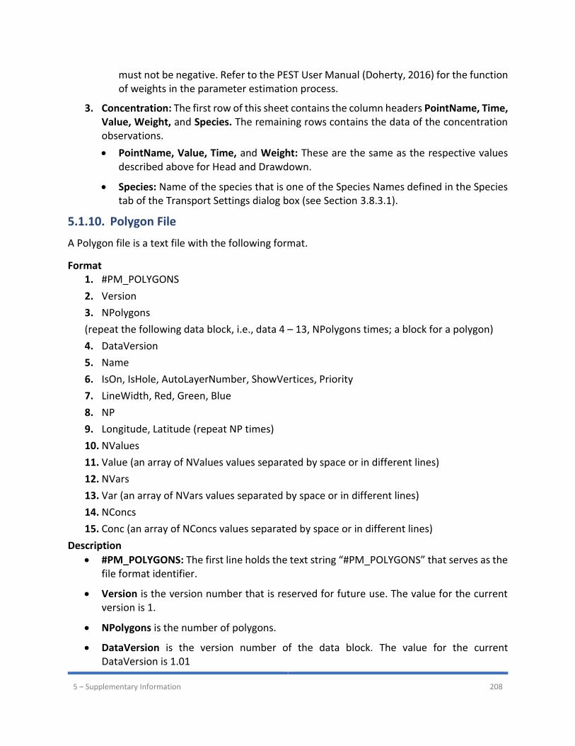
5 – Supplementary Information 208
must not be negative. Refer to the PEST User Manual (Doherty, 2016) for the function of weights in the parameter estimation process.
3. Concentration: The first row of this sheet contains the column headers PointName, Time, Value, Weight, and Species. The remaining rows contains the data of the concentration observations.
• PointName, Value, Time, and Weight: These are the same as the respective values described above for Head and Drawdown.
• Species: Name of the species that is one of the Species Names defined in the Species tab of the Transport Settings dialog box (see Section 3.8.3.1).
5.1.10. Polygon File
A Polygon file is a text file with the following format.
Format 1. #PM_POLYGONS
2. Version
3. NPolygons
(repeat the following data block, i.e., data 4 – 13, NPolygons times; a block for a polygon)
4. DataVersion
5. Name
6. IsOn, IsHole, AutoLayerNumber, ShowVertices, Priority
7. LineWidth, Red, Green, Blue
8. NP
9. Longitude, Latitude (repeat NP times)
10. NValues
11. Value (an array of NValues values separated by space or in different lines)
12. NVars
13. Var (an array of NVars values separated by space or in different lines)
14. NConcs
15. Conc (an array of NConcs values separated by space or in different lines)
Description
• #PM_POLYGONS: The first line holds the text string “#PM_POLYGONS” that serves as the file format identifier.
• Version is the version number that is reserved for future use. The value for the current version is 1.
• NPolygons is the number of polygons.
• DataVersion is the version number of the data block. The value for the current DataVersion is 1.01
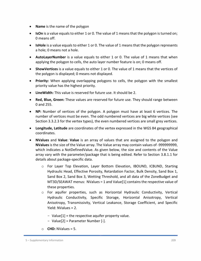
5 – Supplementary Information 209
• Name is the name of the polygon
• IsOn is a value equals to either 1 or 0. The value of 1 means that the polygon is turned on; 0 means off.
• IsHole is a value equals to either 1 or 0. The value of 1 means that the polygon represents a hole; 0 means not a hole.
• AutoLayerNumber is a value equals to either 1 or 0. The value of 1 means that when applying the polygon to cells, the auto layer number feature is on; 0 means off.
• ShowVertices is a value equals to either 1 or 0. The value of 1 means that the vertices of the polygon is displayed; 0 means not displayed.
• Priority: When applying overlapping polygons to cells, the polygon with the smallest priority value has the highest priority.
• LineWidth: This value is reserved for future use. It should be 2.
• Red, Blue, Green: These values are reserved for future use. They should range between 0 and 255.
• NP: Number of vertices of the polygon. A polygon must have at least 6 vertices. The number of vertices must be even. The odd numbered vertices are big white vertices (see Section 3.3.2.3 for the vertex types), the even numbered vertices are small grey vertices.
• Longitude, Latitude are coordinates of the vertex expressed in the WGS 84 geographical coordinates.
• NValues and Value: Value is an array of values that are assigned to the polygon and NValues is the size of the Value array. The Value array may contain values of -999999999, which indicates a NotDefinedValue. As given below, the size and contents of the Value array vary with the parameter/package that is being edited. Refer to Section 3.8.1.1 for details about package-specific data.
o For Layer Top Elevation, Layer Bottom Elevation, IBOUND, ICBUND, Starting
Hydraulic Head, Effective Porosity, Retardation Factor, Bulk Density, Sand Box 1,
Sand Box 2, Sand Box 3, Wetting Threshold, and all data of the ZoneBudget and
MT3D/SEAWAT menus: NValues = 1 and Value[1] contains the respective value of
these properties.
o For aquifer properties, such as Horizontal Hydraulic Conductivity, Vertical
Hydraulic Conductivity, Specific Storage, Horizontal Anisotropy, Vertical
Anisotropy, Transmissivity, Vertical Leakance, Storage Coefficient, and Specific
Yield: NValues = 2.
Value[1] = the respective aquifer property value.
Value[2] = Parameter Number [-].
o CHD: NValues = 5.
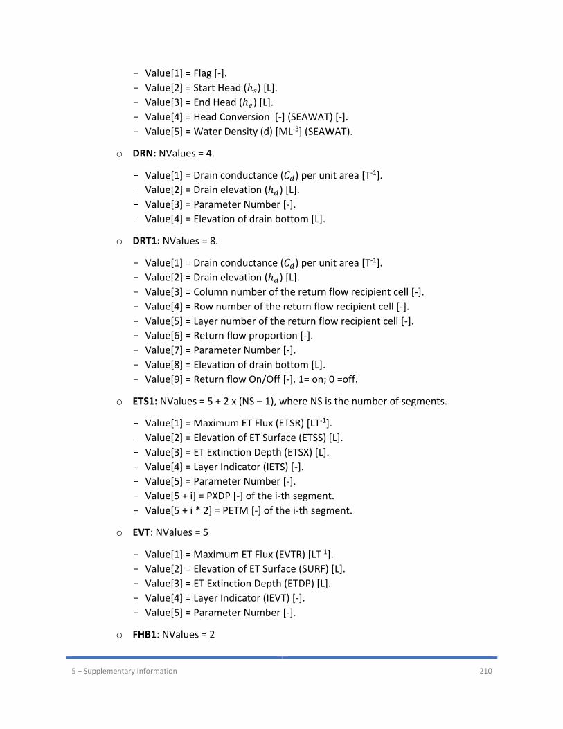
5 – Supplementary Information 210
Value[1] = Flag [-].
Value[2] = Start Head (ℎ𝑠) [L].
Value[3] = End Head (ℎ𝑒) [L].
Value[4] = Head Conversion [-] (SEAWAT) [-].
Value[5] = Water Density (d) [ML-3] (SEAWAT).
o DRN: NValues = 4.
Value[1] = Drain conductance (𝐶𝑑) per unit area [T-1].
Value[2] = Drain elevation (ℎ𝑑) [L].
Value[3] = Parameter Number [-].
Value[4] = Elevation of drain bottom [L].
o DRT1: NValues = 8.
Value[1] = Drain conductance (𝐶𝑑) per unit area [T-1].
Value[2] = Drain elevation (ℎ𝑑) [L].
Value[3] = Column number of the return flow recipient cell [-].
Value[4] = Row number of the return flow recipient cell [-].
Value[5] = Layer number of the return flow recipient cell [-].
Value[6] = Return flow proportion [-].
Value[7] = Parameter Number [-].
Value[8] = Elevation of drain bottom [L].
Value[9] = Return flow On/Off [-]. 1= on; 0 =off.
o ETS1: NValues = 5 + 2 x (NS – 1), where NS is the number of segments.
Value[1] = Maximum ET Flux (ETSR) [LT-1].
Value[2] = Elevation of ET Surface (ETSS) [L].
Value[3] = ET Extinction Depth (ETSX) [L].
Value[4] = Layer Indicator (IETS) [-].
Value[5] = Parameter Number [-].
Value[5 + i] = PXDP [-] of the i-th segment.
Value[5 + i * 2] = PETM [-] of the i-th segment.
o EVT: NValues = 5
Value[1] = Maximum ET Flux (EVTR) [LT-1].
Value[2] = Elevation of ET Surface (SURF) [L].
Value[3] = ET Extinction Depth (ETDP) [L].
Value[4] = Layer Indicator (IEVT) [-].
Value[5] = Parameter Number [-].
o FHB1: NValues = 2
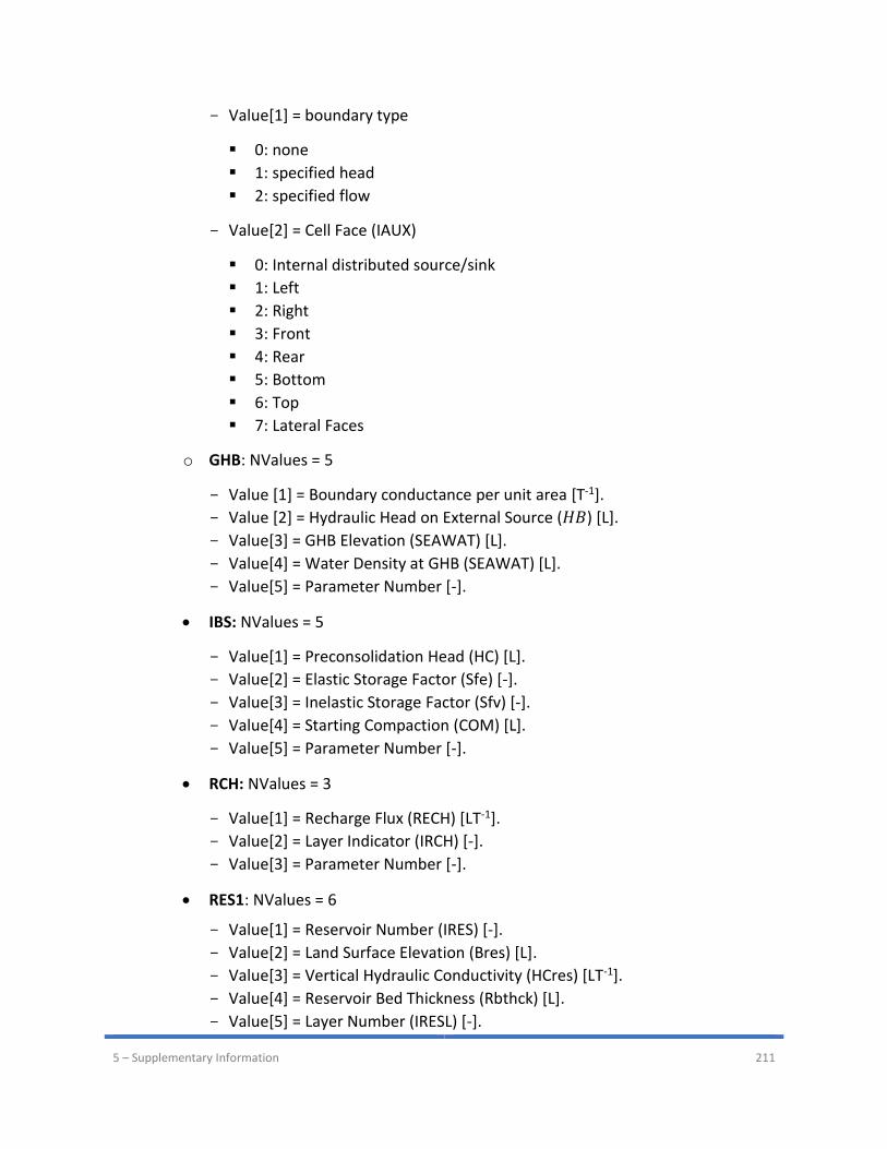
5 – Supplementary Information 211
Value[1] = boundary type
▪ 0: none
▪ 1: specified head
▪ 2: specified flow
Value[2] = Cell Face (IAUX)
▪ 0: Internal distributed source/sink
▪ 1: Left
▪ 2: Right
▪ 3: Front
▪ 4: Rear
▪ 5: Bottom
▪ 6: Top
▪ 7: Lateral Faces
o GHB: NValues = 5
Value [1] = Boundary conductance per unit area [T-1].
Value [2] = Hydraulic Head on External Source (𝐻𝐵) [L].
Value[3] = GHB Elevation (SEAWAT) [L].
Value[4] = Water Density at GHB (SEAWAT) [L].
Value[5] = Parameter Number [-].
• IBS: NValues = 5
Value[1] = Preconsolidation Head (HC) [L].
Value[2] = Elastic Storage Factor (Sfe) [-].
Value[3] = Inelastic Storage Factor (Sfv) [-].
Value[4] = Starting Compaction (COM) [L].
Value[5] = Parameter Number [-].
• RCH: NValues = 3
Value[1] = Recharge Flux (RECH) [LT-1].
Value[2] = Layer Indicator (IRCH) [-].
Value[3] = Parameter Number [-].
• RES1: NValues = 6
Value[1] = Reservoir Number (IRES) [-].
Value[2] = Land Surface Elevation (Bres) [L].
Value[3] = Vertical Hydraulic Conductivity (HCres) [LT-1].
Value[4] = Reservoir Bed Thickness (Rbthck) [L].
Value[5] = Layer Number (IRESL) [-].
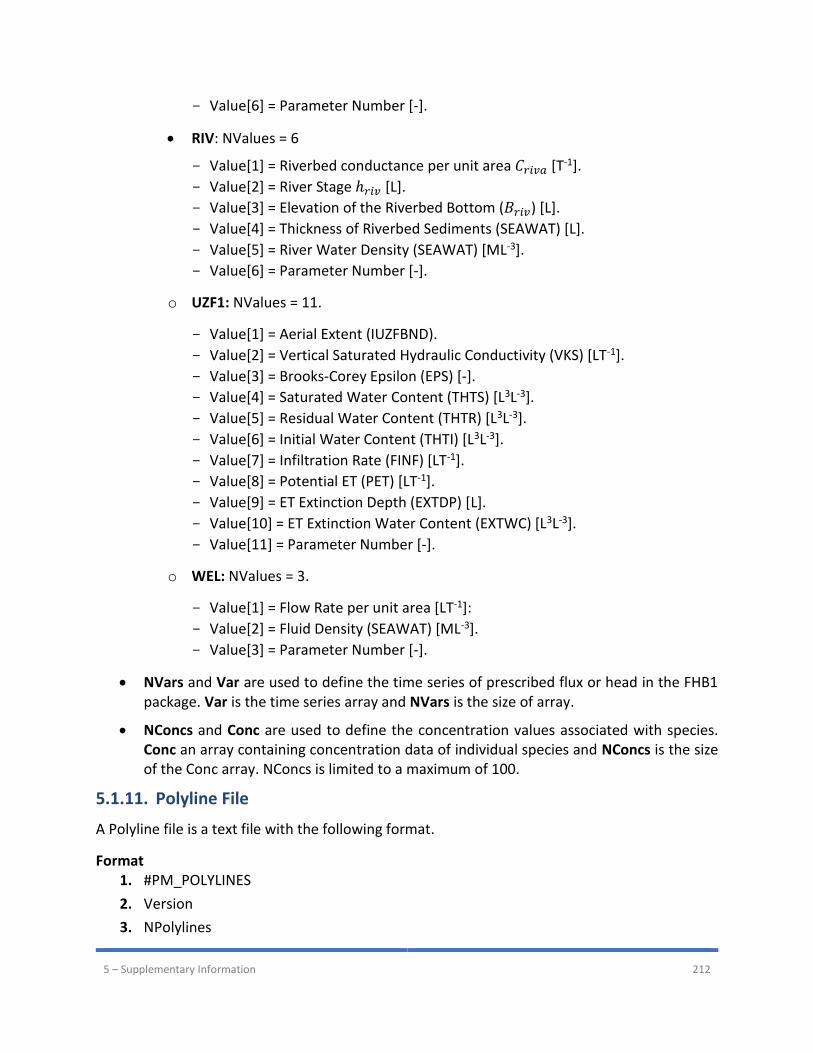
5 – Supplementary Information 212
Value[6] = Parameter Number [-].
• RIV: NValues = 6
Value[1] = Riverbed conductance per unit area 𝐶𝑟𝑖𝑣𝑎 [T-1].
Value[2] = River Stage ℎ𝑟𝑖𝑣 [L].
Value[3] = Elevation of the Riverbed Bottom (𝐵𝑟𝑖𝑣) [L].
Value[4] = Thickness of Riverbed Sediments (SEAWAT) [L].
Value[5] = River Water Density (SEAWAT) [ML-3].
Value[6] = Parameter Number [-].
o UZF1: NValues = 11.
Value[1] = Aerial Extent (IUZFBND).
Value[2] = Vertical Saturated Hydraulic Conductivity (VKS) [LT-1].
Value[3] = Brooks-Corey Epsilon (EPS) [-].
Value[4] = Saturated Water Content (THTS) [L3L-3].
Value[5] = Residual Water Content (THTR) [L3L-3].
Value[6] = Initial Water Content (THTI) [L3L-3].
Value[7] = Infiltration Rate (FINF) [LT-1].
Value[8] = Potential ET (PET) [LT-1].
Value[9] = ET Extinction Depth (EXTDP) [L].
Value[10] = ET Extinction Water Content (EXTWC) [L3L-3].
Value[11] = Parameter Number [-].
o WEL: NValues = 3.
Value[1] = Flow Rate per unit area [LT-1]:
Value[2] = Fluid Density (SEAWAT) [ML-3].
Value[3] = Parameter Number [-].
• NVars and Var are used to define the time series of prescribed flux or head in the FHB1 package. Var is the time series array and NVars is the size of array.
• NConcs and Conc are used to define the concentration values associated with species. Conc an array containing concentration data of individual species and NConcs is the size of the Conc array. NConcs is limited to a maximum of 100.
5.1.11. Polyline File
A Polyline file is a text file with the following format.
Format 1. #PM_POLYLINES
2. Version
3. NPolylines
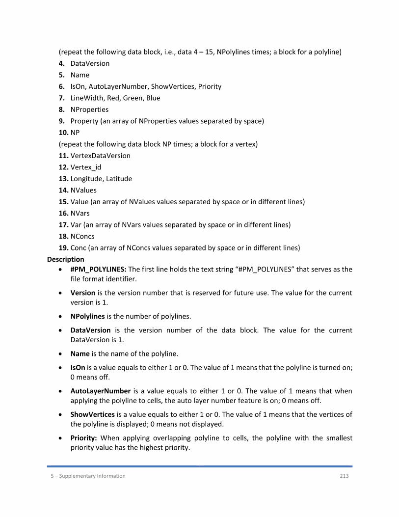
5 – Supplementary Information 213
(repeat the following data block, i.e., data 4 – 15, NPolylines times; a block for a polyline)
4. DataVersion
5. Name
6. IsOn, AutoLayerNumber, ShowVertices, Priority
7. LineWidth, Red, Green, Blue
8. NProperties
9. Property (an array of NProperties values separated by space)
10. NP
(repeat the following data block NP times; a block for a vertex)
11. VertexDataVersion
12. Vertex_id
13. Longitude, Latitude
14. NValues
15. Value (an array of NValues values separated by space or in different lines)
16. NVars
17. Var (an array of NVars values separated by space or in different lines)
18. NConcs
19. Conc (an array of NConcs values separated by space or in different lines)
Description
• #PM_POLYLINES: The first line holds the text string “#PM_POLYLINES” that serves as the file format identifier.
• Version is the version number that is reserved for future use. The value for the current version is 1.
• NPolylines is the number of polylines.
• DataVersion is the version number of the data block. The value for the current DataVersion is 1.
• Name is the name of the polyline.
• IsOn is a value equals to either 1 or 0. The value of 1 means that the polyline is turned on; 0 means off.
• AutoLayerNumber is a value equals to either 1 or 0. The value of 1 means that when applying the polyline to cells, the auto layer number feature is on; 0 means off.
• ShowVertices is a value equals to either 1 or 0. The value of 1 means that the vertices of the polyline is displayed; 0 means not displayed.
• Priority: When applying overlapping polyline to cells, the polyline with the smallest priority value has the highest priority.
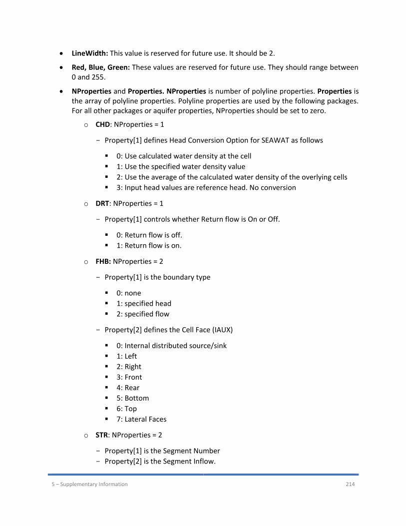
5 – Supplementary Information 214
• LineWidth: This value is reserved for future use. It should be 2.
• Red, Blue, Green: These values are reserved for future use. They should range between 0 and 255.
• NProperties and Properties. NProperties is number of polyline properties. Properties is the array of polyline properties. Polyline properties are used by the following packages. For all other packages or aquifer properties, NProperties should be set to zero.
o CHD: NProperties = 1
Property[1] defines Head Conversion Option for SEAWAT as follows
▪ 0: Use calculated water density at the cell
▪ 1: Use the specified water density value
▪ 2: Use the average of the calculated water density of the overlying cells
▪ 3: Input head values are reference head. No conversion
o DRT: NProperties = 1
Property[1] controls whether Return flow is On or Off.
▪ 0: Return flow is off.
▪ 1: Return flow is on.
o FHB: NProperties = 2
Property[1] is the boundary type
▪ 0: none
▪ 1: specified head
▪ 2: specified flow
Property[2] defines the Cell Face (IAUX)
▪ 0: Internal distributed source/sink
▪ 1: Left
▪ 2: Right
▪ 3: Front
▪ 4: Rear
▪ 5: Bottom
▪ 6: Top
▪ 7: Lateral Faces
o STR: NProperties = 2
Property[1] is the Segment Number
Property[2] is the Segment Inflow.

5 – Supplementary Information 215
• NP: Number of vertices of the polyline. A polyline must have at least 3 vertices. The number of vertices must be odd. The odd numbered vertices are big white vertices (see Section 3.3.2.3 for the vertex types), the even numbered vertices are small grey vertices.
• VertexDataVersion is the version number of the vertex block. The value for the current VertexDataVersion is 1.01.
• Vertex_id, introduced since VertexDataVersion 1.01, is the unique identifier of the vertex.
• Longitude, Latitude are coordinates of the vertex expressed in the WGS 84 geographical coordinates.
• NValues and Value: Value is an array of values that are assigned to the vertex. NValues is the size of the Value array. Note that a Value array may only be assigned to odd numbered vertices. Values that are assigned to even numbered vertices will be discarded. The Value array may contain values of -999999999, which indicates a NotDefinedValue. As given below, the size and contents of the Value array vary with the parameter/package that is being edited. Refer to Section 3.8.1.1 for details about package-specific data.
o For Layer Top Elevation, Layer Bottom Elevation, IBOUND, ICBUND, Starting
Hydraulic Head, Effective Porosity, Retardation Factor, Bulk Density, Sand Box 1,
Sand Box 2, Sand Box 3, Wetting Threshold, and all data of the ZoneBudget and
MT3D/SEAWAT menus: NValues = 1 and Value[1] contains the respective value of
these properties.
o For aquifer properties, such as Horizontal Hydraulic Conductivity, Vertical
Hydraulic Conductivity, Specific Storage, Horizontal Anisotropy, Vertical
Anisotropy, Transmissivity, Vertical Leakance, Storage Coefficient, and Specific
Yield: NValues = 2.
Value[1] = the respective aquifer property value.
Value[2] = Parameter Number [-].
o DRN: NValues = 4.
Value[1] = Drain conductance per unit length [LT-1].
Value[2] = Drain elevation (ℎ𝑑) [L].
Value[3] = Parameter Number [-].
Value[4] = Elevation of drain bottom [L].
o DRT1: NValues = 8.
Value[1] = Drain conductance per unit length [LT-1].
Value[2] = Drain elevation (ℎ𝑑) [L].
Value[3] = Column number of the return flow recipient cell [-].
Value[4] = Row number of the return flow recipient cell [-].
Value[5] = Layer number of the return flow recipient cell [-].
Value[6] = Return flow proportion [-].
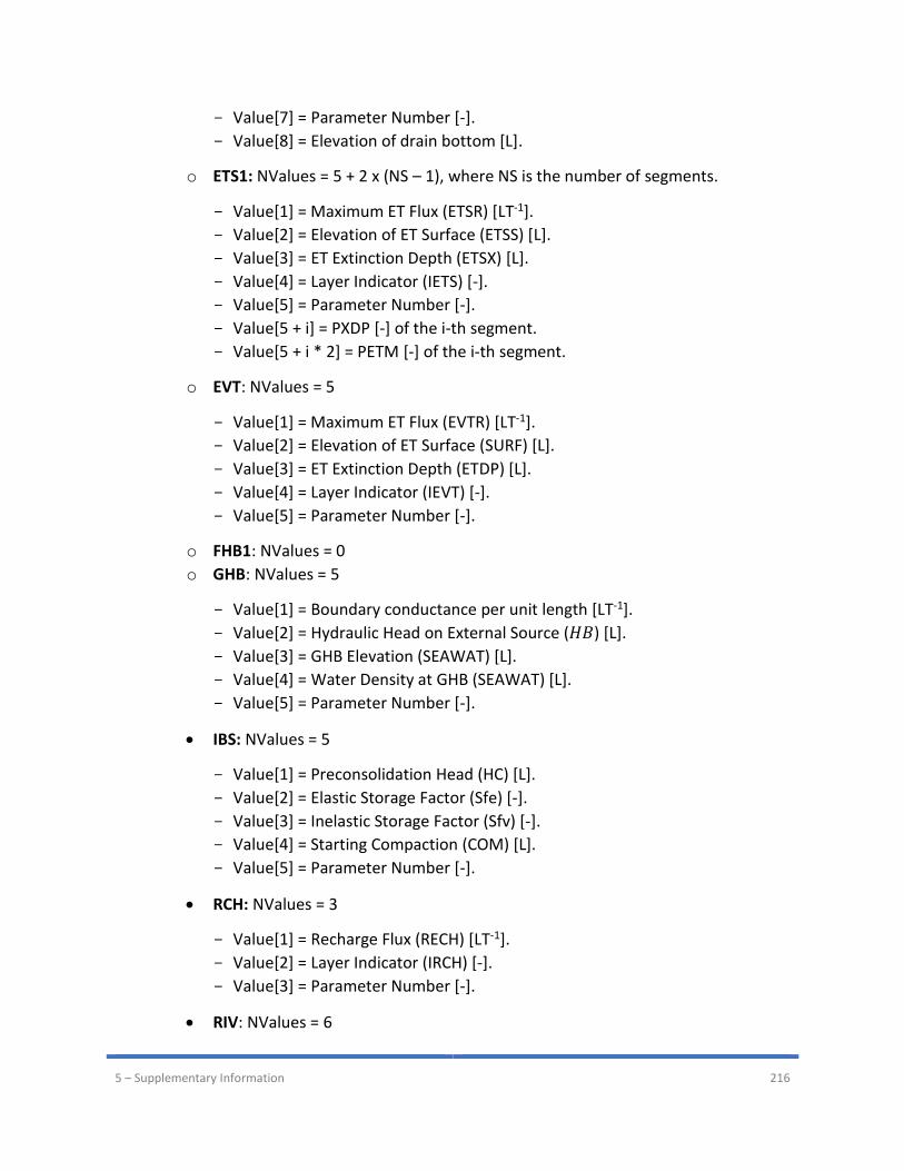
5 – Supplementary Information 216
Value[7] = Parameter Number [-].
Value[8] = Elevation of drain bottom [L].
o ETS1: NValues = 5 + 2 x (NS – 1), where NS is the number of segments.
Value[1] = Maximum ET Flux (ETSR) [LT-1].
Value[2] = Elevation of ET Surface (ETSS) [L].
Value[3] = ET Extinction Depth (ETSX) [L].
Value[4] = Layer Indicator (IETS) [-].
Value[5] = Parameter Number [-].
Value[5 + i] = PXDP [-] of the i-th segment.
Value[5 + i * 2] = PETM [-] of the i-th segment.
o EVT: NValues = 5
Value[1] = Maximum ET Flux (EVTR) [LT-1].
Value[2] = Elevation of ET Surface (SURF) [L].
Value[3] = ET Extinction Depth (ETDP) [L].
Value[4] = Layer Indicator (IEVT) [-].
Value[5] = Parameter Number [-].
o FHB1: NValues = 0
o GHB: NValues = 5
Value[1] = Boundary conductance per unit length [LT-1].
Value[2] = Hydraulic Head on External Source (𝐻𝐵) [L].
Value[3] = GHB Elevation (SEAWAT) [L].
Value[4] = Water Density at GHB (SEAWAT) [L].
Value[5] = Parameter Number [-].
• IBS: NValues = 5
Value[1] = Preconsolidation Head (HC) [L].
Value[2] = Elastic Storage Factor (Sfe) [-].
Value[3] = Inelastic Storage Factor (Sfv) [-].
Value[4] = Starting Compaction (COM) [L].
Value[5] = Parameter Number [-].
• RCH: NValues = 3
Value[1] = Recharge Flux (RECH) [LT-1].
Value[2] = Layer Indicator (IRCH) [-].
Value[3] = Parameter Number [-].
• RIV: NValues = 6
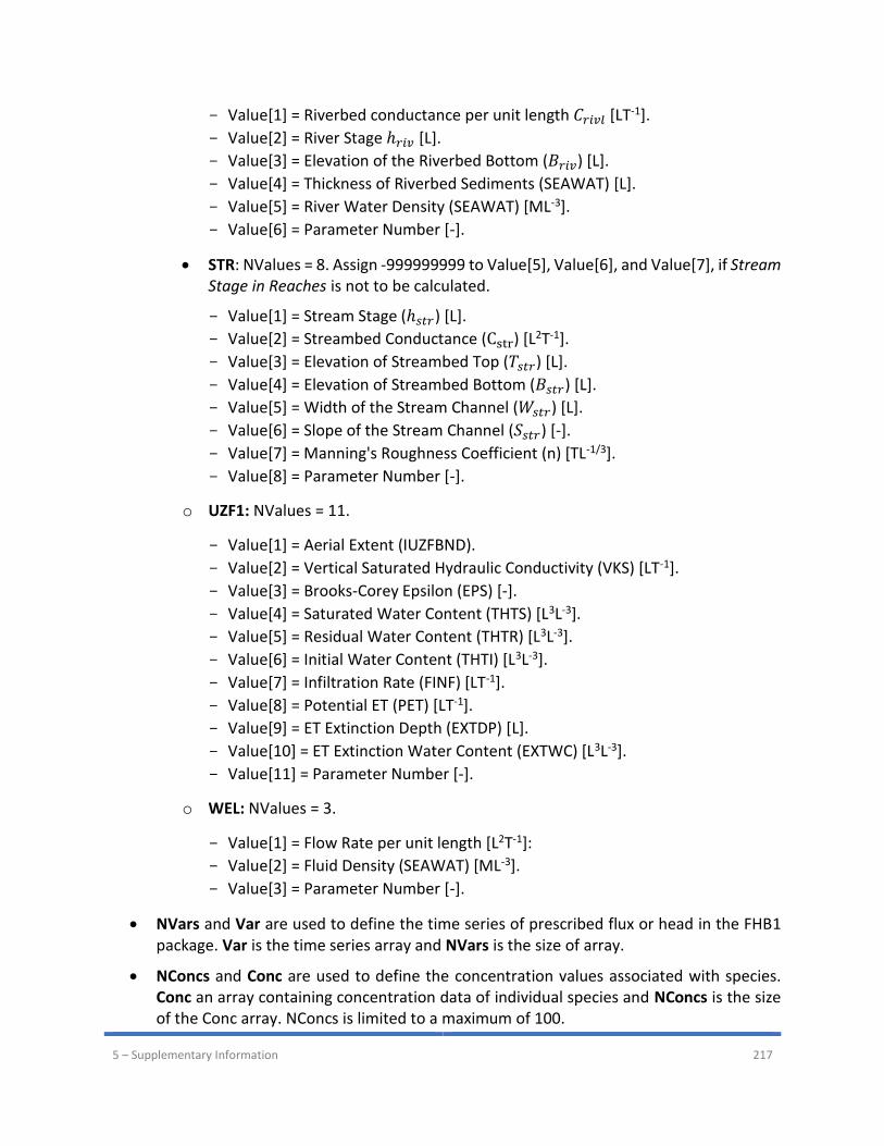
5 – Supplementary Information 217
Value[1] = Riverbed conductance per unit length 𝐶𝑟𝑖𝑣𝑙 [LT-1].
Value[2] = River Stage ℎ𝑟𝑖𝑣 [L].
Value[3] = Elevation of the Riverbed Bottom (𝐵𝑟𝑖𝑣) [L].
Value[4] = Thickness of Riverbed Sediments (SEAWAT) [L].
Value[5] = River Water Density (SEAWAT) [ML-3].
Value[6] = Parameter Number [-].
• STR: NValues = 8. Assign -999999999 to Value[5], Value[6], and Value[7], if Stream Stage in Reaches is not to be calculated.
Value[1] = Stream Stage (ℎ𝑠𝑡𝑟) [L].
Value[2] = Streambed Conductance (Cstr) [L2T-1].
Value[3] = Elevation of Streambed Top (𝑇𝑠𝑡𝑟) [L].
Value[4] = Elevation of Streambed Bottom (𝐵𝑠𝑡𝑟) [L].
Value[5] = Width of the Stream Channel (𝑊𝑠𝑡𝑟) [L].
Value[6] = Slope of the Stream Channel (𝑆𝑠𝑡𝑟) [-].
Value[7] = Manning's Roughness Coefficient (n) [TL-1/3].
Value[8] = Parameter Number [-].
o UZF1: NValues = 11.
Value[1] = Aerial Extent (IUZFBND).
Value[2] = Vertical Saturated Hydraulic Conductivity (VKS) [LT-1].
Value[3] = Brooks-Corey Epsilon (EPS) [-].
Value[4] = Saturated Water Content (THTS) [L3L-3].
Value[5] = Residual Water Content (THTR) [L3L-3].
Value[6] = Initial Water Content (THTI) [L3L-3].
Value[7] = Infiltration Rate (FINF) [LT-1].
Value[8] = Potential ET (PET) [LT-1].
Value[9] = ET Extinction Depth (EXTDP) [L].
Value[10] = ET Extinction Water Content (EXTWC) [L3L-3].
Value[11] = Parameter Number [-].
o WEL: NValues = 3.
Value[1] = Flow Rate per unit length [L2T-1]:
Value[2] = Fluid Density (SEAWAT) [ML-3].
Value[3] = Parameter Number [-].
• NVars and Var are used to define the time series of prescribed flux or head in the FHB1 package. Var is the time series array and NVars is the size of array.
• NConcs and Conc are used to define the concentration values associated with species. Conc an array containing concentration data of individual species and NConcs is the size of the Conc array. NConcs is limited to a maximum of 100.

5 – Supplementary Information 218
5.1.12. Reservoir Stage Time Series
A Reservoir Stage Time Series file is a text file that contains the stage measurements of reservoirs.
Format 1. #RESERVOIR_STAGE_SERIES
2. Version
3. NRES
(repeat the following block NRES times)
4. ReserviorNumber, ReservoirName
5. N
(repeat the following line N times)
6. Time, Stage
Description
• #RESERVOIR_STAGE_SERIES: The first line holds the text string “#RESERVOIR_STAGE_SERIES” that serves as the file format identifier.
• Version is the version number that is reserved for future use. The value for the current version is 1.
• NRES is the number of reservoirs.
• ReserviorNumber and ReservoirName are the number and name of the reservoir, respectively.
• N is the number of data points that will follow.
• Time and Stage are the model elapsed time and the reservoir stage, respectively.
5.1.13. Series File
A Series file is a text file that contains a series of numbers.
Format 1. #SERIES
2. Version
3. N
4. v(1) v(2) v3 …. v(N)
Description
• #SERIES: The first line holds the text string ”#SERIES” that serves as the file format identifier.
• Version is the version number that is reserved for future use. The value for the current version is 1.
• N is the number of values that will follow.
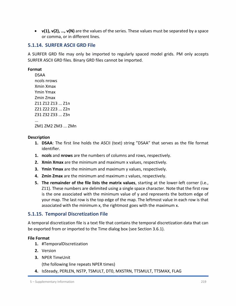
5 – Supplementary Information 219
• v(1), v(2), …, v(N) are the values of the series. These values must be separated by a space or comma, or in different lines.
5.1.14. SURFER ASCII GRD File
A SURFER GRD file may only be imported to regularly spaced model grids. PM only accepts
SURFER ASCII GRD files. Binary GRD files cannot be imported.
Format DSAA ncols nrows Xmin Xmax Ymin Ymax Zmin Zmax Z11 Z12 Z13 ... Z1n Z21 Z22 Z23 ... Z2n Z31 Z32 Z33 ... Z3n ... ZM1 ZM2 ZM3 ... ZMn
Description
1. DSAA: The first line holds the ASCII (text) string ”DSAA” that serves as the file format identifier.
1. ncols and nrows are the numbers of columns and rows, respectively.
2. Xmin Xmax are the minimum and maximum x values, respectively.
3. Ymin Ymax are the minimum and maximum y values, respectively.
4. Zmin Zmax are the minimum and maximum z values, respectively.
5. The remainder of the file lists the matrix values, starting at the lower-left corner (i.e., Z11). These numbers are delimited using a single space character. Note that the first row is the one associated with the minimum value of y and represents the bottom edge of your map. The last row is the top edge of the map. The leftmost value in each row is that associated with the minimum x, the rightmost goes with the maximum x.
5.1.15. Temporal Discretization File
A temporal discretization file is a text file that contains the temporal discretization data that can
be exported from or imported to the Time dialog box (see Section 3.6.1).
File Format 1. #TemporalDiscretization
2. Version
3. NPER TimeUnit
(the following line repeats NPER times)
4. IsSteady, PERLEN, NSTP, TSMULT, DT0, MXSTRN, TTSMULT, TTSMAX, FLAG
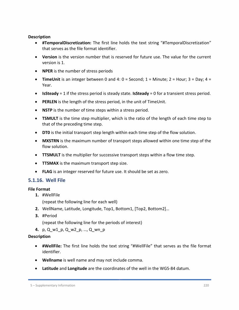
5 – Supplementary Information 220
Description
• #TemporalDiscretization: The first line holds the text string “#TemporalDiscretization” that serves as the file format identifier.
• Version is the version number that is reserved for future use. The value for the current version is 1.
• NPER is the number of stress periods
• TimeUnit is an integer between 0 and 4: 0 = Second; 1 = Minute; 2 = Hour; 3 = Day; 4 = Year.
• IsSteady = 1 if the stress period is steady state. IsSteady = 0 for a transient stress period.
• PERLEN is the length of the stress period, in the unit of TimeUnit.
• NSTP is the number of time steps within a stress period.
• TSMULT is the time step multiplier, which is the ratio of the length of each time step to that of the preceding time step.
• DT0 is the initial transport step length within each time step of the flow solution.
• MXSTRN is the maximum number of transport steps allowed within one time step of the flow solution.
• TTSMULT is the multiplier for successive transport steps within a flow time step.
• TTSMAX is the maximum transport step size.
• FLAG is an integer reserved for future use. It should be set as zero.
5.1.16. Well File
File Format 1. #WellFile
(repeat the following line for each well)
2. WellName, Latitude, Longitude, Top1, Bottom1, [Top2, Bottom2]…
3. #Period
(repeat the following line for the periods of interest)
4. p, Q_w1_p, Q_w2_p, …, Q_wn_p
Description
• #WellFile: The first line holds the text string “#WellFile” that serves as the file format identifier.
• Wellname is well name and may not include comma.
• Latitude and Longitude are the coordinates of the well in the WGS-84 datum.
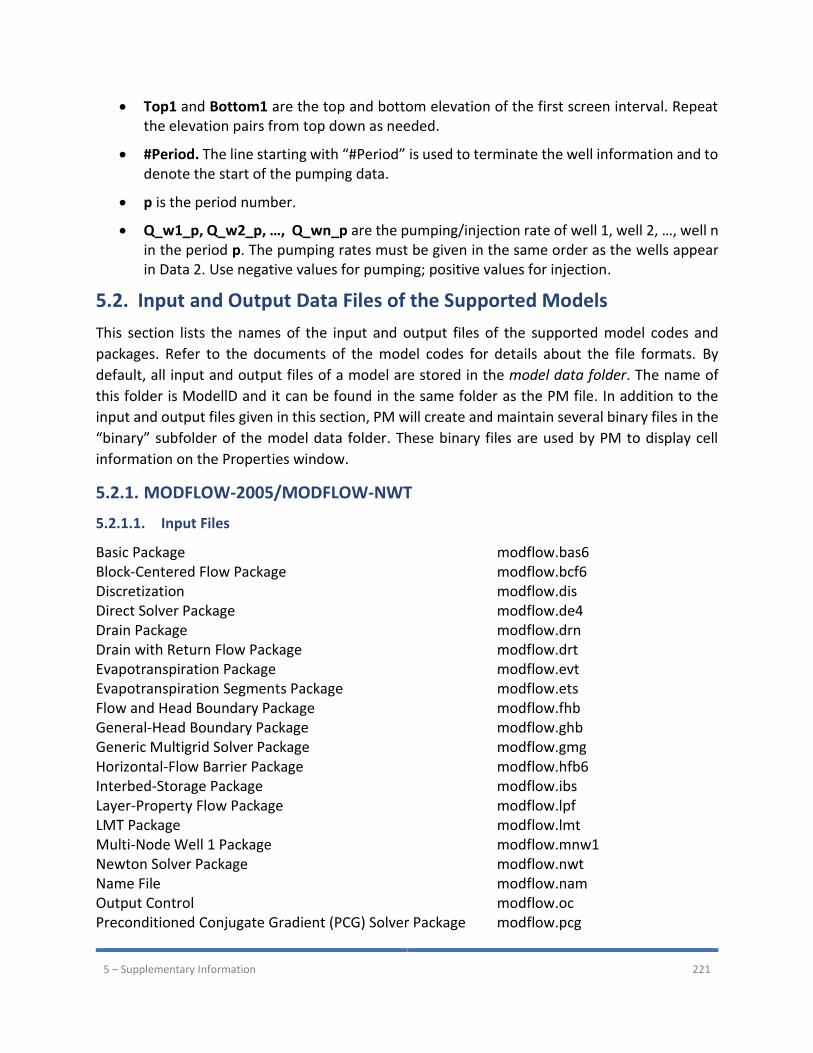
5 – Supplementary Information 221
• Top1 and Bottom1 are the top and bottom elevation of the first screen interval. Repeat the elevation pairs from top down as needed.
• #Period. The line starting with “#Period” is used to terminate the well information and to denote the start of the pumping data.
• p is the period number.
• Q_w1_p, Q_w2_p, …, Q_wn_p are the pumping/injection rate of well 1, well 2, …, well n in the period p. The pumping rates must be given in the same order as the wells appear in Data 2. Use negative values for pumping; positive values for injection.
5.2. Input and Output Data Files of the Supported Models
This section lists the names of the input and output files of the supported model codes and
packages. Refer to the documents of the model codes for details about the file formats. By
default, all input and output files of a model are stored in the model data folder. The name of
this folder is ModellD and it can be found in the same folder as the PM file. In addition to the
input and output files given in this section, PM will create and maintain several binary files in the
“binary” subfolder of the model data folder. These binary files are used by PM to display cell
information on the Properties window.
5.2.1. MODFLOW-2005/MODFLOW-NWT
5.2.1.1. Input Files
Basic Package modflow.bas6 Block-Centered Flow Package modflow.bcf6 Discretization modflow.dis Direct Solver Package modflow.de4 Drain Package modflow.drn Drain with Return Flow Package modflow.drt Evapotranspiration Package modflow.evt Evapotranspiration Segments Package modflow.ets Flow and Head Boundary Package modflow.fhb General-Head Boundary Package modflow.ghb Generic Multigrid Solver Package modflow.gmg Horizontal-Flow Barrier Package modflow.hfb6 Interbed-Storage Package modflow.ibs Layer-Property Flow Package modflow.lpf LMT Package modflow.lmt Multi-Node Well 1 Package modflow.mnw1 Newton Solver Package modflow.nwt Name File modflow.nam Output Control modflow.oc Preconditioned Conjugate Gradient (PCG) Solver Package modflow.pcg
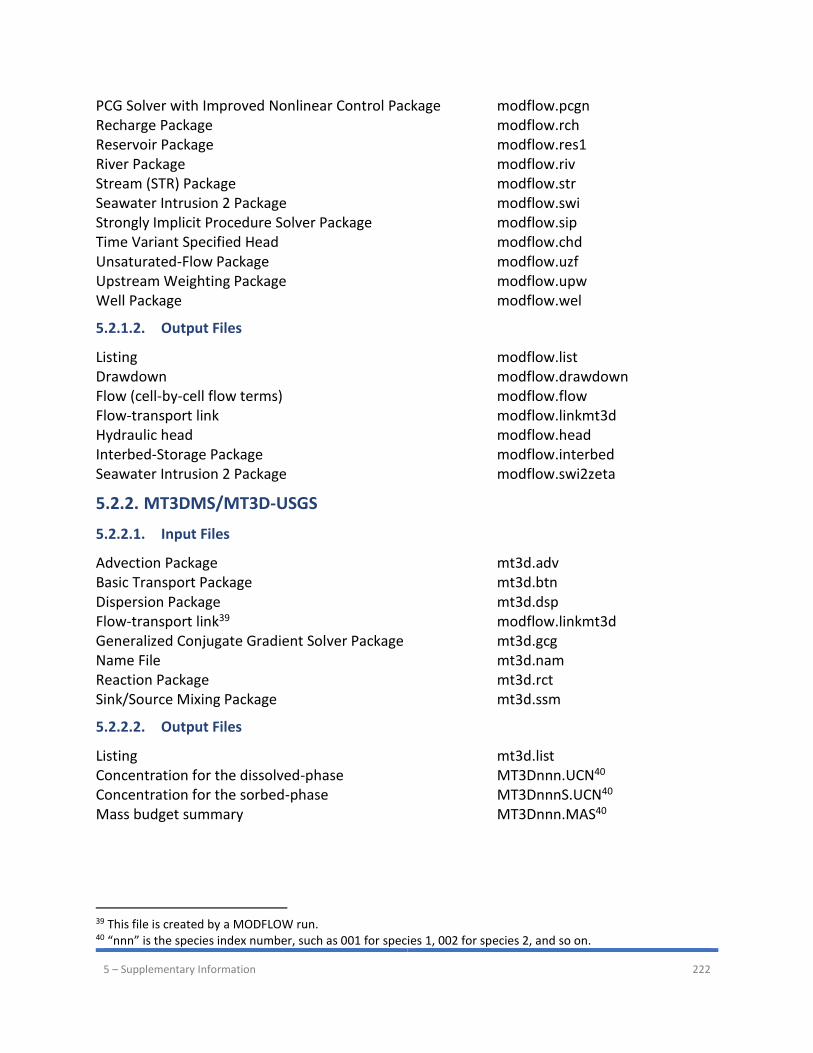
5 – Supplementary Information 222
PCG Solver with Improved Nonlinear Control Package modflow.pcgn Recharge Package modflow.rch Reservoir Package modflow.res1 River Package modflow.riv Stream (STR) Package modflow.str Seawater Intrusion 2 Package modflow.swi Strongly Implicit Procedure Solver Package modflow.sip Time Variant Specified Head modflow.chd Unsaturated-Flow Package modflow.uzf Upstream Weighting Package modflow.upw Well Package modflow.wel
5.2.1.2. Output Files
Listing modflow.list Drawdown modflow.drawdown Flow (cell-by-cell flow terms) modflow.flow Flow-transport link modflow.linkmt3d Hydraulic head modflow.head Interbed-Storage Package modflow.interbed Seawater Intrusion 2 Package modflow.swi2zeta
5.2.2. MT3DMS/MT3D-USGS
5.2.2.1. Input Files
Advection Package mt3d.adv Basic Transport Package mt3d.btn Dispersion Package mt3d.dsp Flow-transport link39 modflow.linkmt3d Generalized Conjugate Gradient Solver Package mt3d.gcg Name File mt3d.nam Reaction Package mt3d.rct Sink/Source Mixing Package mt3d.ssm
5.2.2.2. Output Files
Listing mt3d.list Concentration for the dissolved-phase MT3Dnnn.UCN40 Concentration for the sorbed-phase MT3DnnnS.UCN40 Mass budget summary MT3Dnnn.MAS40
39 This file is created by a MODFLOW run. 40 “nnn” is the species index number, such as 001 for species 1, 002 for species 2, and so on.
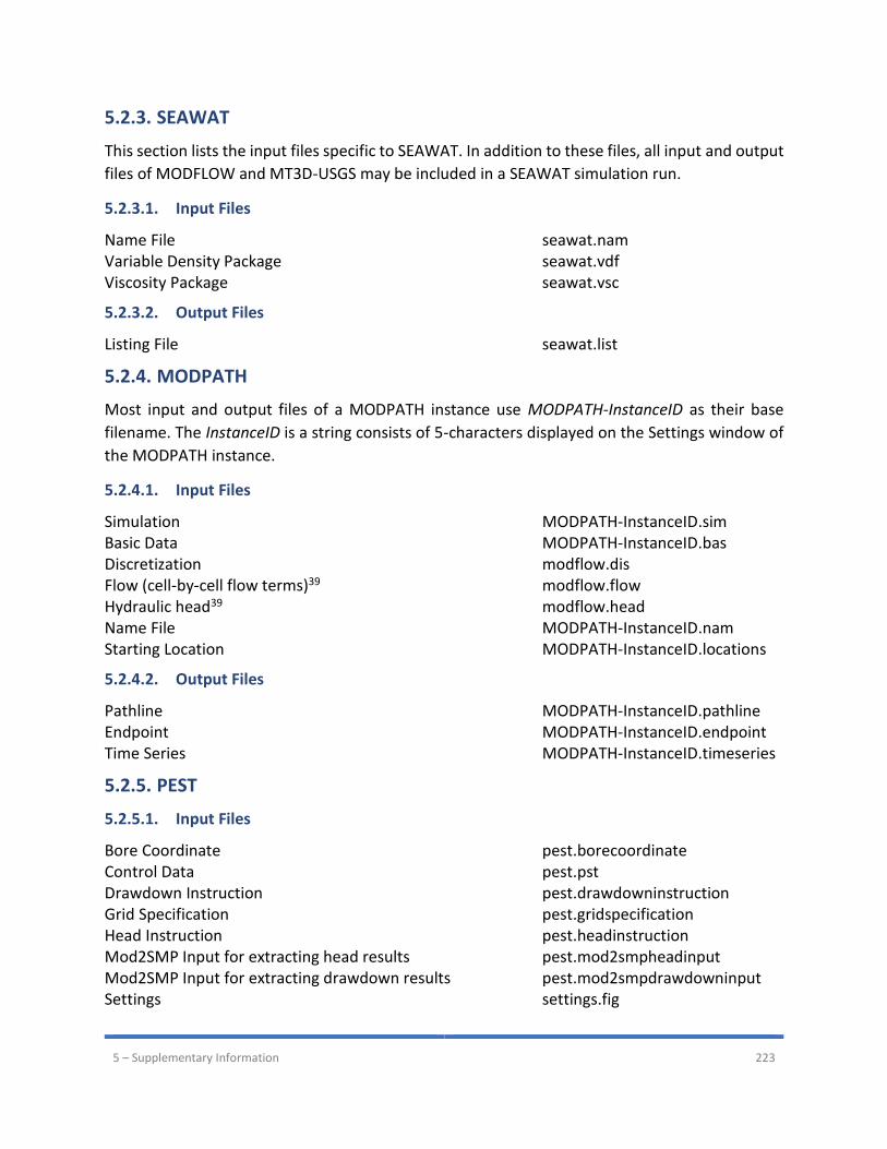
5 – Supplementary Information 223
5.2.3. SEAWAT
This section lists the input files specific to SEAWAT. In addition to these files, all input and output
files of MODFLOW and MT3D-USGS may be included in a SEAWAT simulation run.
5.2.3.1. Input Files
Name File seawat.nam Variable Density Package seawat.vdf Viscosity Package seawat.vsc
5.2.3.2. Output Files
Listing File seawat.list
5.2.4. MODPATH
Most input and output files of a MODPATH instance use MODPATH-InstanceID as their base
filename. The InstanceID is a string consists of 5-characters displayed on the Settings window of
the MODPATH instance.
5.2.4.1. Input Files
Simulation MODPATH-InstanceID.sim Basic Data MODPATH-InstanceID.bas Discretization modflow.dis Flow (cell-by-cell flow terms)39 modflow.flow Hydraulic head39 modflow.head Name File MODPATH-InstanceID.nam Starting Location MODPATH-InstanceID.locations
5.2.4.2. Output Files
Pathline MODPATH-InstanceID.pathline Endpoint MODPATH-InstanceID.endpoint Time Series MODPATH-InstanceID.timeseries
5.2.5. PEST
5.2.5.1. Input Files
Bore Coordinate pest.borecoordinate Control Data pest.pst Drawdown Instruction pest.drawdowninstruction Grid Specification pest.gridspecification Head Instruction pest.headinstruction Mod2SMP Input for extracting head results pest.mod2smpheadinput Mod2SMP Input for extracting drawdown results pest.mod2smpdrawdowninput Settings settings.fig
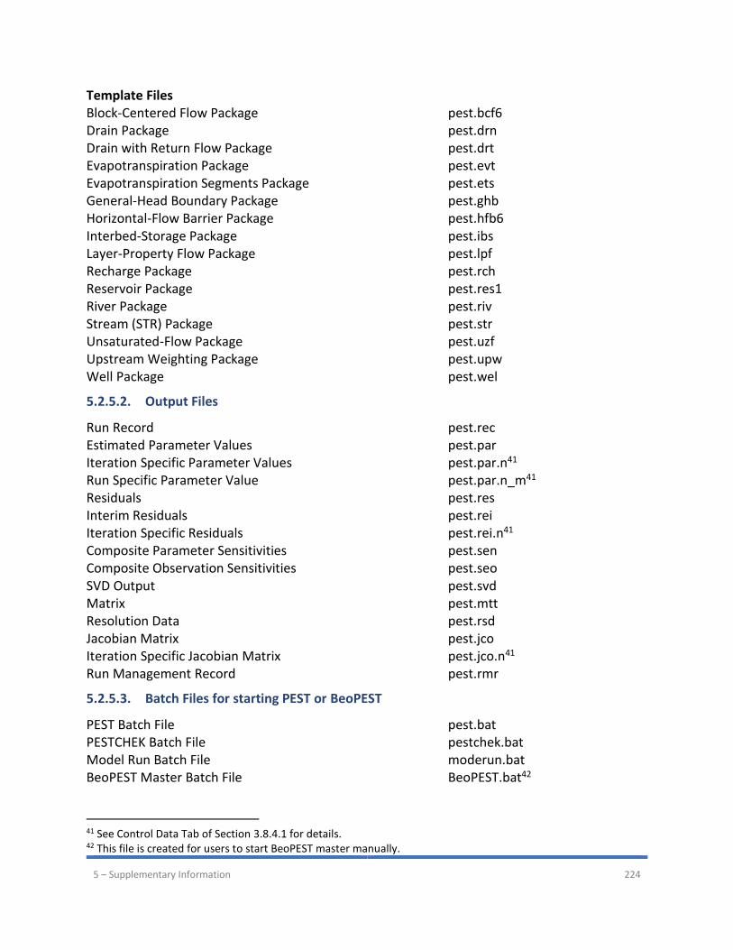
5 – Supplementary Information 224
Template Files Block-Centered Flow Package pest.bcf6 Drain Package pest.drn Drain with Return Flow Package pest.drt Evapotranspiration Package pest.evt Evapotranspiration Segments Package pest.ets General-Head Boundary Package pest.ghb Horizontal-Flow Barrier Package pest.hfb6 Interbed-Storage Package pest.ibs Layer-Property Flow Package pest.lpf Recharge Package pest.rch Reservoir Package pest.res1 River Package pest.riv Stream (STR) Package pest.str Unsaturated-Flow Package pest.uzf Upstream Weighting Package pest.upw Well Package pest.wel
5.2.5.2. Output Files
Run Record pest.rec Estimated Parameter Values pest.par Iteration Specific Parameter Values pest.par.n41 Run Specific Parameter Value pest.par.n_m41 Residuals pest.res Interim Residuals pest.rei Iteration Specific Residuals pest.rei.n41 Composite Parameter Sensitivities pest.sen Composite Observation Sensitivities pest.seo SVD Output pest.svd Matrix pest.mtt Resolution Data pest.rsd Jacobian Matrix pest.jco Iteration Specific Jacobian Matrix pest.jco.n41 Run Management Record pest.rmr
5.2.5.3. Batch Files for starting PEST or BeoPEST
PEST Batch File pest.bat PESTCHEK Batch File pestchek.bat Model Run Batch File moderun.bat BeoPEST Master Batch File BeoPEST.bat42
41 See Control Data Tab of Section 3.8.4.1 for details. 42 This file is created for users to start BeoPEST master manually.

5 – Supplementary Information 225
BeoPEST Agent Batch File BeoPEST_slave.bat43 BeoPEST Agents Batch File BeoPEST_slaves.bat44
43 This batch file starts an instance of BeoPEST agent. 44 This batch file starts all instances of BeoPEST agent.
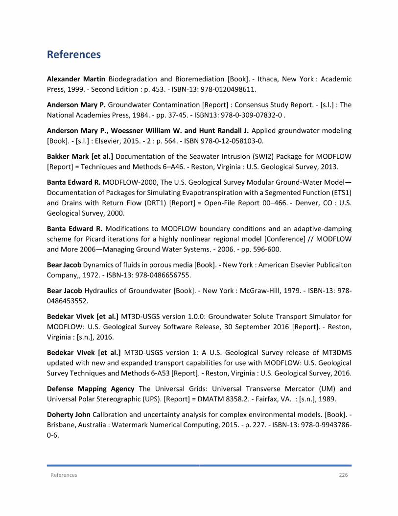
References 226
References
Alexander Martin Biodegradation and Bioremediation [Book]. - Ithaca, New York : Academic
Press, 1999. - Second Edition : p. 453. - ISBN-13: 978-0120498611.
Anderson Mary P. Groundwater Contamination [Report] : Consensus Study Report. - [s.l.] : The
National Academies Press, 1984. - pp. 37-45. - ISBN13: 978-0-309-07832-0 .
Anderson Mary P., Woessner William W. and Hunt Randall J. Applied groundwater modeling
[Book]. - [s.l.] : Elsevier, 2015. - 2 : p. 564. - ISBN 978-0-12-058103-0.
Bakker Mark [et al.] Documentation of the Seawater Intrusion (SWI2) Package for MODFLOW
[Report] = Techniques and Methods 6–A46. - Reston, Virginia : U.S. Geological Survey, 2013.
Banta Edward R. MODFLOW-2000, The U.S. Geological Survey Modular Ground-Water Model—
Documentation of Packages for Simulating Evapotranspiration with a Segmented Function (ETS1)
and Drains with Return Flow (DRT1) [Report] = Open-File Report 00–466. - Denver, CO : U.S.
Geological Survey, 2000.
Banta Edward R. Modifications to MODFLOW boundary conditions and an adaptive-damping
scheme for Picard iterations for a highly nonlinear regional model [Conference] // MODFLOW
and More 2006—Managing Ground Water Systems. - 2006. - pp. 596-600.
Bear Jacob Dynamics of fluids in porous media [Book]. - New York : American Elsevier Publicaiton
Company,, 1972. - ISBN-13: 978-0486656755.
Bear Jacob Hydraulics of Groundwater [Book]. - New York : McGraw-Hill, 1979. - ISBN-13: 978-
0486453552.
Bedekar Vivek [et al.] MT3D-USGS version 1.0.0: Groundwater Solute Transport Simulator for
MODFLOW: U.S. Geological Survey Software Release, 30 September 2016 [Report]. - Reston,
Virginia : [s.n.], 2016.
Bedekar Vivek [et al.] MT3D-USGS version 1: A U.S. Geological Survey release of MT3DMS
updated with new and expanded transport capabilities for use with MODFLOW: U.S. Geological
Survey Techniques and Methods 6-A53 [Report]. - Reston, Virginia : U.S. Geological Survey, 2016.
Defense Mapping Agency The Universal Grids: Universal Transverse Mercator (UM) and
Universal Polar Stereographic (UPS). [Report] = DMATM 8358.2. - Fairfax, VA. : [s.n.], 1989.
Doherty John Calibration and uncertainty analysis for complex environmental models. [Book]. -
Brisbane, Australia : Watermark Numerical Computing, 2015. - p. 227. - ISBN-13: 978-0-9943786-
0-6.
References 227
Doherty John Model-Independent Parameter Estimation User Manual: 6th Edition. [Report]. -
Brisbane, Australia : Water Numerical Computing, 2016.
Doherty John MODINV - Suite of software for MODFLOW pre-processing, postprocessing and
parameter optimization. User’s manual. [Report]. - Australia : Australian Centre for Tropical
Research, 1990.
Domenico Patrick A. and Schwartz Franklin W. Physical and Chemical Hydrogeology [Book]. -
[s.l.] : John Wiley & Sons, Inc., 1997. - 2nd. - ISBN-13: 978-0471597629.
Domenico Patrick A. Concepts and Models in Groundwater Hydrology [Book]. - [s.l.] : McGraw-
Hill, 1972. - ISBN: 978-0070175358.
ESRI ESRI Shapefile Technical Description -- An ESRI White Paper [Online] // ESRI.COM. - July
1998. - July 17, 2017. - https://www.esri.com/library/whitepapers/pdfs/shapefile.pdf.
Fenske Jon P., Leake Stanley A. and Prudic David E. Documentation of a computer program
(RES1) to simulate leakage from reservoirs using the modular finite-difference ground-water flow
model (MODFLOW) [Report] = Open-File Report 96-364. - Tucson, Arizona : U.S. Geological
Survey, 1996.
Fetter Charles W. Applied Hydrogeology [Book]. - [s.l.] : Prentice-Hall, 1994. - 3rd Edition : p.
691. - ISBN: 978-0023364907.
Freeze Allan R. and Cherry John A. Groundwater [Book]. - Upper Saddle River, NJ : Prentice-Hall,
Inc., 1979. - ISBN 978-0133653120.
Gelhar Lynn W., Welty Claire and Rehfeldt Kenneth R. A critical review of data on field-scale
dispersion in aquifers [Journal]. - [s.l.] : Water Resources Research, 1992. - 7 : Vol. 28.
Gesch D. [et al.] The National Elevation Dataset [Journal] // Photopragrammtric Engineering &
Remote Sensing. - [s.l.] : ASPRS, 2002. - 1 : Vol. 68.
Goodin William R., McRae Gregory J. and Seinfeld John H. A compaison of interpolation methods
for sparse data: application to wind and concentration fields. [Journal] // Journal of Applied
Meteorology and Climatology. - [s.l.] : American Meteorological Society, June 1979. - Vol. 18. -
pp. 761-771.
Guo Weixing and Langevin Christian D. User's guide to SEAWAT; a computer program for
simulation of three-dimensional variable-density ground-water flow [Report] = Techniques of
Water-Resources Investigations 06-A7. - Tallahassee, Florida : U.S. Geological Survey, 2002.
Halford Keith J. and Hanson Randall T User Guide for the Drawdown-Limited, Multi-Node Well
(MNW) Package for the U.S. Geological Survey’s Modular Three-Dimensional Finite-Difference
Ground-Water Flow Model,Versions MODFLOW-96 and MODFLOW-2000 [Report] = Open-File
Report 02-293. - Sacramento, California : U. S. Geological Survey, 2002.
References 228
Harbaugh Arlen W. [et al.] MODFLOW-2000, The U.S. Geological Survey modular ground-water
model -- User guide to modularization concepts and the ground-water flow process.Open-File
Report 00-92 [Report]. - Reston, Virginia : U.S. GEOLOGICAL SURVEY, 2000.
Harbaugh Arlen W. A Computer Program for Calculating Subregional Water Budgets Using
Results from the U.S. Geological Survey Modular Three-dimensional Finite-difference Ground-
water Flow Model. Open-File Report 90-392 [Report] = Open-File Report 90-392. - Reston,
Virginia : U.S. Geological Survey, 1990. - p. 49.
Harbaugh Arlen W. and McDonald Michael G. User’s documentation for MODFLOW-96, an
update to the U.S. Geological Survey modular finite-difference ground-water flow model. Open-
File Report 96-485 [Report]. - Reston, Virginia : U.S. GEOLOGICAL SURVEY , 1996.
Harbaugh Arlen W. Direct solution package based on alternating diagonal ordering for the U.S.
Geological Survey modular finite-difference ground-water flow model [Report] = Open File
Report 95-288. - Reston, Virginia : U.S. Geological Survey, 1995.
Harbaugh Arlen W. MODFLOW-2005, the U.S. Geological Survey modular ground-water model -
- the Ground-Water Flow Process: Techniques and Methods 6-A16. [Report]. - Reston, Virginia :
U.S. Geological Survey, 2005.
Hill Mary C. Preconditioned Conjugate-Gradient 2 (PCG2), A Computer Program for Solving
Ground-Water Flow Equations [Report] = Water-Resources Investigations Report 90-4048. -
Denver, Colorado : U.S. Geological Survey, 1990.
Hsieh Paul A. and Freckleton John R. Documentation of a computer program to simulate
horizontal-flow barriers using the U.S. Geological Survey’s modular three dimensional finite-
difference ground-water flow model [Report] = Open-File Report 92–477. - Sacramento,
California : U. S. Geological Survey, 1993.
Hunt Randall J. [et al.] Using the cloud to replenish parched groundwater modeling efforts. Rapid
Communication for Ground Water, doi: 10.1111/j.1745-6584.2010.00699 [Journal] // Ground
Water. - [s.l.] : Ground Water, 2010. - 3 : Vol. 48. - pp. 360-365.
Langevin C.D., Thorne D.T., Jr. and Dausman A.M. SEAWAT Version 4: A Computer Program for
Simulation of Multi-Species Solute and Heat Transport: U.S. Geological Survey Techniques and
Methods Book 6, Chapter A22, 39 p. [Report]. - Reston, Virginia : U.S. Geological Survey, 2007.
Langevin Christian D. [et al.] MODFLOW 6 Modular Hydrologic Model version 6.0.0 [Report] =
Techniques and Methods 6–A55. - Reston, Virginia : U.S. Geological Survey, 2017.
Leake Stanley A. and Prudic David E. Documentation of a computer program to simulate aquifer-
system compaction using the modular finite-difference ground-water flow model [Report] =
Techniques of Water-Resources Investigations 06-A2. - [s.l.] : U. S. Geological Survey, 1991.
References 229
Leake Stanley. A. and Lilly Michael R. Documentation of a Computer Program (FHB1) for
Assignment of Transient Specified-Flow and Specified-Head Boundaries in Applications of the
Modular Finite-Difference Ground-Water Flow Model (MODFLOW) [Report] = Open-File Report
97-571. - Tucson, Arizona : U. S. Geological Survey, 1997.
Leonard B. P. A stable and accurate convective modeling procedure based on quadratic upstream
interpolation. [Journal]. - [s.l.] : Computer Methods in Applied Mechanics and Engineering,
1979. - Vol. 19. - pp. 59-98.
Leonard B. P. Universal Limiter for transient interpolation modeling of the advective transport
equations: the ULTIMATE conservative difference scheme [Report] = NASA Technical
Memorandum 100916 ICOMP-88-11 / Institute for Computational Mechanics in Propulsion Lewis
Research Center. - Cleveland, Ohio : NASA, 1988.
McDonald Michael G. and Harbaugh Arlen W. MODFLOW, A modular three-dimensional finite
difference ground-water flow model [Report] = TWRI-6-A1. - Reston, Virginia : U. S. Geological
Survey, 1988.
McDonald Michael G. [et al.] A method of converting no-flow cells to variable-head cells for the
U. S. Geological Survey modular finite-difference ground-water flow model [Report] = Open-File
Report 91-536. - [s.l.] : U. S. Geological Survey, 1991.
Mehl Steffen W. and Mary Hill C. MODFLOW-2000, the U. S. Geological Survey modular ground-
water model; user guide to the Link-AMG (LMG) package for solving matrix equations using an
algebraic multigrid solver [Report] = Open-File Report 2001-177. - Denver, Colorado : U. S.
Geological Survey, 2001.
Naff Richard L. and Banta Edward R. The U.S. Geological Survey Modular Ground-Water Model
- PCGN: A Preconditioned Conjugate Gradient Solver with Improved Nonlinear Control [Report] =
Open-File Report 2008-1331. - Reston, Virginia : U. S. Geological Survey, 2008.
National Imagery and Mapping Agency Department of Defense World Geodetic System 1984.
Its Definition and Relationships with Local Geodetic Systems. [Report] = NIMA TR8350.2. Third
Edition. - 1984.
Neville Christopher J. Interpreting the MT3D Mass Budget [Online] // www.sspa.com. - S.S.
Papadopulos, Inc., June 7, 2006. - February 19, 2018. -
http://www.sspa.com/sites/default/files/images/stories/documents/MT3D-notes_mass-
budget.pdf.
Niswonger Richard G., Panday Sorab and Ibaraki Motomu MODFLOW-NWT, A Newton
formulation for MODFLOW-2005: U.S. Geological Survey Techniques and Methods 6-A37, 44 p.
[Report]. - Reston, Virginia : U.S. Geological Survey, 2011.
References 230
Niswonger Richard G., Prudic David E. and Regan Steven R. Documentation of the Unsaturated-
Zone Flow (UZF1) Package for Modeling Unsaturated Flow Between the Land Surface and the
Water Table with MODFLOW-2005 [Report] = Techniques and Methods 6-A19. - Reston, Virginia :
[s.n.], 2006.
Peaceman Donald W. Interpretation of well-block pressures in numerical reservoir simulation
with nonsquare grid blocks and anisotropic permeability [Journal]. - [s.l.] : Society of Petroleum
Engineers Journal, June 1983. - 3 : Vol. 23. - pp. 531–543.
Pollock David W. User guide for MODPATH Version 7 -- A particle-tracking model for MODFLOW:
U.S. Geological Survey Open-File Report 2016-1086, 35 p.,
http://dx.doi.org/10.3133/ofr20161086. [Report]. - Reston, Virginia : U.S. Geological Survey,
2016.
Prudic David E. Documentation of a computer program to simulate stream-aquifer relations
using a modular, finite-difference, ground-water flow model [Report] = Open-File Report 88-
729. - Carson City, Nevada : U. S. Geological Survey, 1989.
Schwartz Joe Understanding Bing Maps -- Bing Maps Tile System. [Online] // MSDN Library. -
2010. - July 17, 2017. - http://msdn.microsoft.com/en-us/library/bb259689.aspx.
Shepard D. A two dimensional interpolation function for irregularly spaced data. [Conference] //
126 ACM National Conference. - 1968. - pp. 517-524.
Spitz Karlheinz and Moreno Joanna A Practical Guide to Groundwater and Solute Transport
Modeling [Book]. - [s.l.] : Wiley, 1996. - ISBN: 978-0-471-13687-3.
Wilson John D. and Naff Richard L. MODFLOW¬2000, The U.S. Geological Survey Modular
Ground¬Water Model – GMG Linear Equation Solver Package Documentation [Report] = Open-
File Report 2004-1261 / U. S. Geological Survey. - Denver, Colorado : [s.n.], 2004.
Zheng Chunmiao and Bennett Gordon D. Applied contaminant transport modeling: Theory and
practice [Book]. - New York : Van Nostrand Reinhold, 1995. - 1st : p. 440. - ISBN-13:
9780442013486.
Zheng Chunmiao and Wang Patrick P. MT3DMS: A modular three-dimensional multispecies
Transport Model for Simulation of Advection, Dispersion, and Chemical Reactions of
Contaminants in Groundwater Systems; Documentation and User’s Guide, Contract Report
SERDP-99-1 [Report]. - Vicksburg, MS : U.S. Army Engineer Research and Development Center,
1999.
Index 231
Index
A
active cell ........................................................ 3, 20, 46, 104
active layer .......................................................................... 3
active model........................................................................ 3
animation .......................................................................... 35
anisotropy
horizontal ..................................................................... 61
vertical ......................................................................... 62
B
base maps ......................................................................... 10
BeoPEST .............................................................................. 2
bulk density....................................................................... 64
C
caption ................................................................................ 8
contours
input parameter ......................................................... 188
model results ............................................................. 192
Copy Cell Data ......................................................... 5, 45, 47
Copy Grid Size ............................................................... 6, 48
Copy Grid Split Factor ................................................... 6, 48
Copy Layer Data ...................................................... 5, 45, 47
Cross section ..................................................................... 45
CSV ......................................................... vi, 1, 132, 136, 204
D
Data
export ........................................................................... 52
import .................................................................... 49, 52
modify .......................................................................... 49
data editor .................................................................. 18, 19
diffusion coefficient ........................................................ 153
E
effective porosity .............................................................. 63
ESRI Raster .......................................................................... 1
estimable parameters .................................................... 162
Export ............................................................................... 52
F
First-order Euler ............................................................. 151
flow vectors .................................................................... 194
Fourth-order Runge-Kutta .............................................. 151
G
georeferencing method.................................................... 31
grid azimuth ..................................................................... 31
grid cursor .................................................................... 4, 46
grid editor ................................................................... 17, 18
ground surface elevation ................................................... 4
H
HMOC ............................................................................. 151
hydraulic conductivity
horizontal .................................................................... 61
vertical ......................................................................... 62
I
IBOUND ............................................................................ 60
ICBUND ............................................................................. 60
image .................................................................................. 9
import............................................................................... 49
Import Data ................................................................ 49, 52
Import Package ................................................................ 53
input method
cell-by-cell ............................................................... 5, 20
polygon .................................................................... 5, 24
polyline .................................................................... 5, 21
internal flow packages ..................................................... 29
interpolation .................................................................... 51
L
layer type ......................................................................... 56
longitudinal dispersivity ................................................. 153
Index 232
LSQR ................................................................................ 176
M
MMOC ............................................................................ 150
MOC ................................................................................ 150
model
create ........................................................................... 28
import .......................................................................... 32
model grid
move ............................................................................ 40
rotate ........................................................................... 40
MODFLOW 6 ....................................................................... 2
MODFLOW-2005 ............................................................... 36
MODFLOW-NWT ...... 2, 29, 36, 123, 126, 127, 149, 182, 221
Modify Data ...................................................................... 49
MODINV .............................................................................. 1
MODPATH ....................................................................... 197
MT3DMS ............................................................... 1, 37, 149
N
National Elevation Dataset ................................................. 4
O
observation data ............................................................... 42
observation points ............................................................ 41
OpenStreetMap ................................................................ 10
P
Package
Advection (ADV) ......................................................... 149
Dispersion (DSP) ......................................................... 153
Drain (DRN) .................................................................. 64
Drain with Return Flow (DRT1) .................................... 66
Evapotranspiration (EVT) ............................................. 69
Evapotranspiration Segments (ETS1) ........................... 70
Flow and Head Boundary (FHB1) ................................. 72
General-Head Boundary (GHB) .................................... 76
Horizontal-Flow Barrier (HFB) ...................................... 79
import .......................................................................... 53
Interbed Storage (IBS) .................................................. 80
Multi-Node Well (MNW1) ............................................ 81
Reaction (RCT) ............................................................ 154
Recharge (RCH) ............................................................ 84
Reservoir (RES1) ........................................................... 88
River (RIV) .................................................................... 85
Sink/Source Mixing (SSM) ......................................... 155
Stream (STR) ................................................................ 91
Time-Variant Specified-Head (CHD) .......................... 101
Unsaturated-Zone Flow (UZF1) ................................. 102
Variable-Density Flow (VDF) ...................................... 155
Viscosity (VSC) ........................................................... 155
Well (WEL) ................................................................. 105
parameter group ............................................................ 167
particle-tracking algorithm ............................................. 151
pathlines ......................................................................... 202
PEST ...................................................................... 1, 38, 162
preconditioned conjugate gradient ........................ 116, 118
preferences ...................................................................... 36
prior information ............................................................ 169
prj 12, 34
projection ................................................................... 12, 34
Proxy ................................................................................ 39
Q
quadkey ............................................................................ 11
R
regularization mode ....................................................... 164
retardation factor ............................................................. 63
Run
MODFLOW ................................................................. 126
MODPATH ................................................................. 200
MT3D ......................................................................... 159
PEST ........................................................................... 181
PESTCHEK .................................................................. 182
SEAWAT ..................................................................... 159
ZoneBudget ............................................................... 136
S
sandbox ............................................................................ 64
SEAWAT .........................................................1, 37, 137, 146
seawater intrusion ........................................................... 97
sensitivity analysis .......................................................... 164
Shapefile ................................................................. 1, 12, 50
Solvers
MODFLOW ................................................................. 110
MT3D ......................................................................... 155
PEST ........................................................................... 165
spatial discretization ........................................................ 17
specific storage ................................................................. 62
specific yield ..................................................................... 63
starting hydraulic head ..................................................... 61
Index 233
storage coefficient ............................................................ 62
SVD ................................................................................. 175
T
table of contents ................................................................. 3
temporal discretization ............................................... 17, 54
Tikhonov regularization .................................................. 171
tiled-map services ....................................................... 10, 11
time unit ........................................................................... 54
TOC ..................................................... See table of contents
transmissivity .................................................................... 61
U
ULTIMATE ....................................................................... 149
units .................................................................................. 17
Universal Transverse Mercator ........................................... 4
UTM .................................................................................... 4
V
vertical leakance ............................................................... 62
view .................................................................................... 7
W
Wetting Threshold.......................................................... 108
World file .......................................................................... 35
World Geodetic System 1984 ......................................... vi, 4
Z
Zone Budget ....................................................................... 2