procedural approaches curvestmm/courses/cpsc414-03-fall/vsep2003/slides… · procedural approaches...

University of British ColumbiaUniversity of British Columbia

CPSC 414 Computer GraphicsCPSC 414 Computer Graphics

© Tamara Munzner 1

Procedural ApproachesCurves

Week 12, Fri 21 Nov 2003

Week 12, Fri 21 Nov 03 © Tamara Munzner 2

News• midterm solutions out• late hw2: handin box 18, CICSR basement• project 3 out

• final location announced– LSK 200– noon Tue Dec 9– must have photo ID

• student ID best


Display Technologies recap• mobile display with laser to retina• stereo glasses/display• 3D scanners– laser stripe + camera– laser time-of-flight– cameras only, depth from stereo

• Shape Tape• haptics (Phantom)• 3D printers


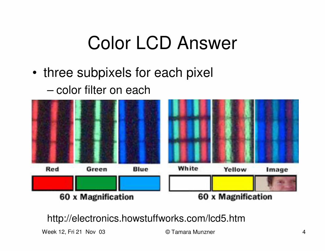
Color LCD Answer• three subpixels for each pixel

– color filter on each

http://electronics.howstuffworks.com/lcd5.htm


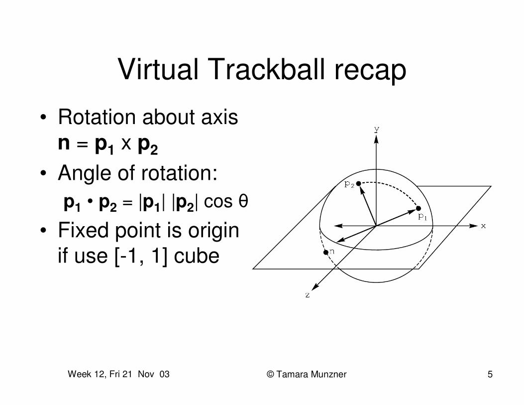
Virtual Trackball recap• Rotation about axis

n = p1 x p2

• Angle of rotation:p1 • p2 = |p1| |p2| cos �

• Fixed point is origin if use [-1, 1] cube



© Tamara Munzner 6

Procedural Approaches


Procedural Modeling• textures, geometry

– explicitly stored in memory

• procedural approach– compute something on the fly– often less memory cost– visual richness

• fractals, particle systems, noise


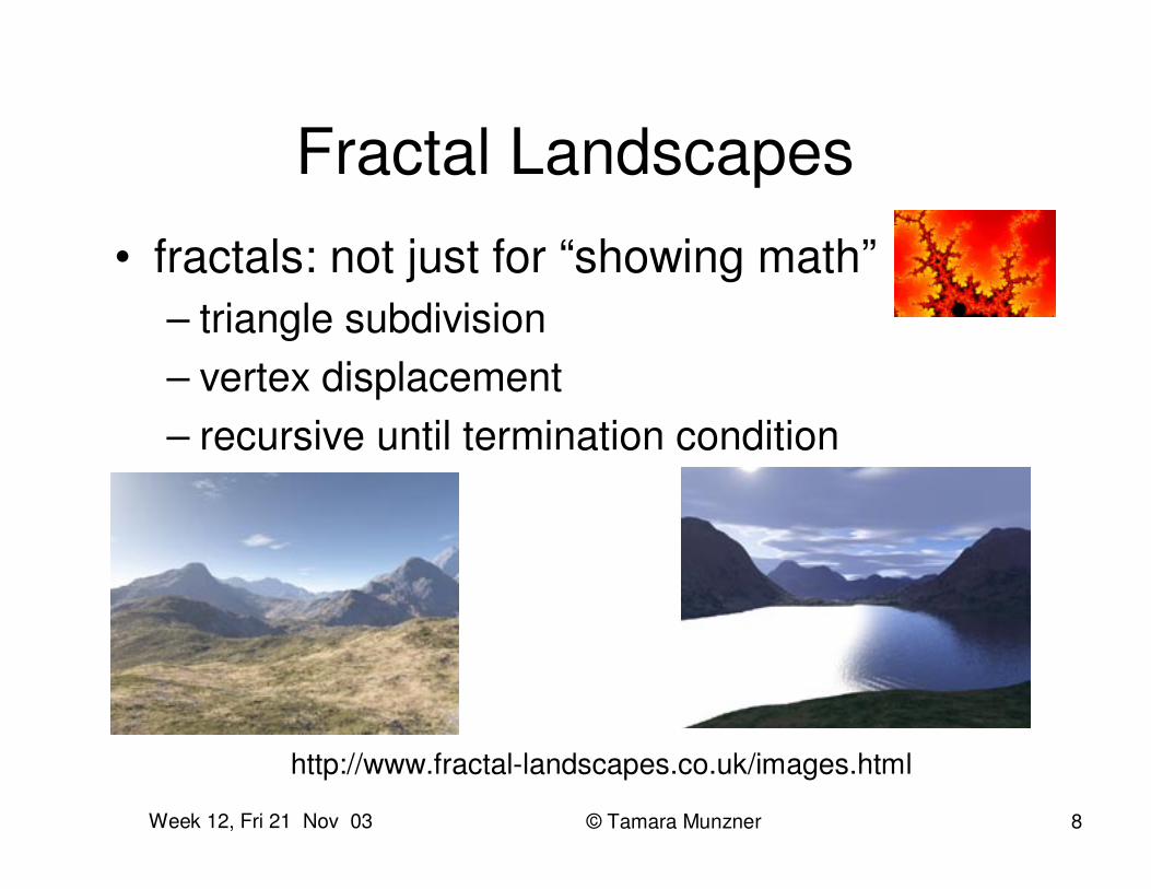
Fractal Landscapes• fractals: not just for “showing math”

– triangle subdivision– vertex displacement– recursive until termination condition

http://www.fractal-landscapes.co.uk/images.html


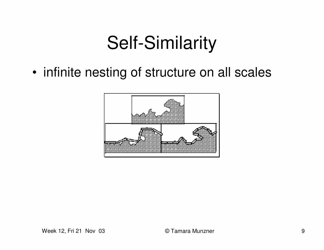
Self-Similarity• infinite nesting of structure on all scales


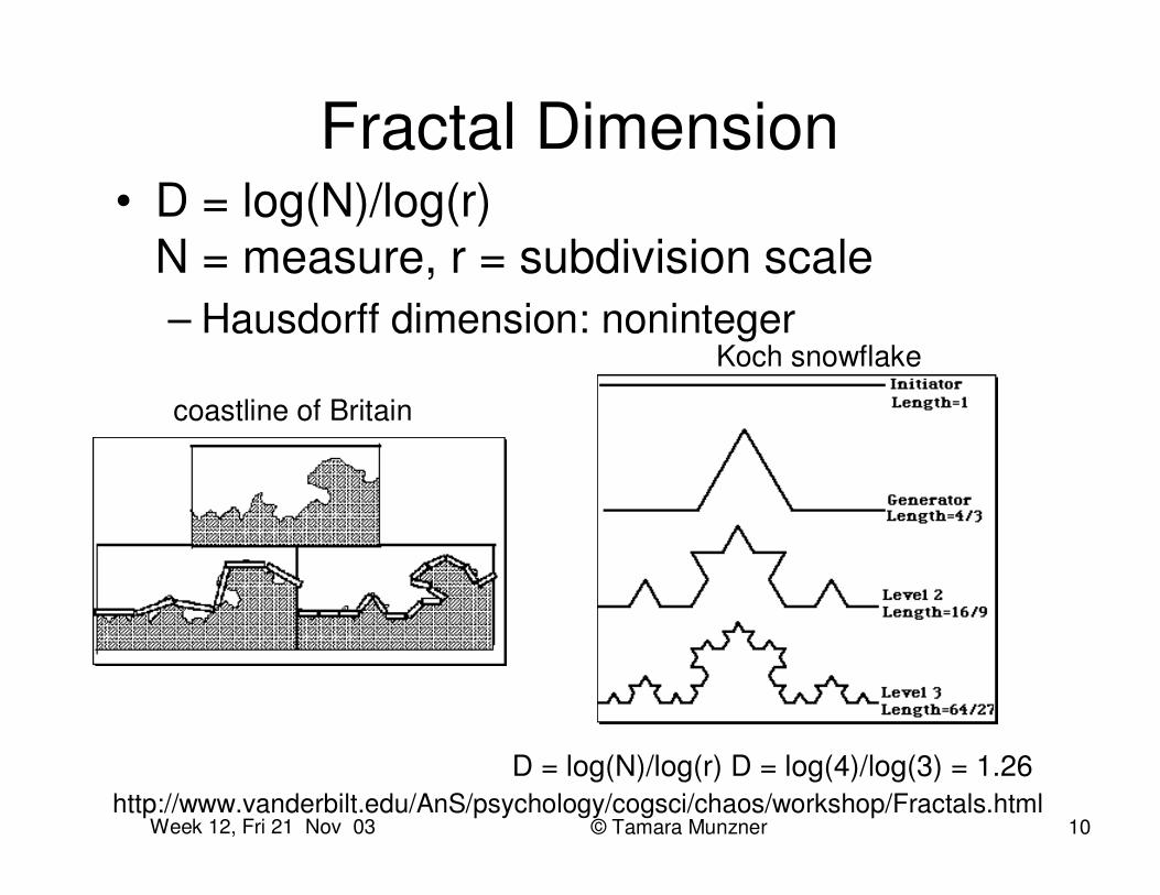
Fractal Dimension• D = log(N)/log(r)

N = measure, r = subdivision scale– Hausdorff dimension: noninteger

D = log(N)/log(r) D = log(4)/log(3) = 1.26

coastline of Britain

Koch snowflake

http://www.vanderbilt.edu/AnS/psychology/cogsci/chaos/workshop/Fractals.html


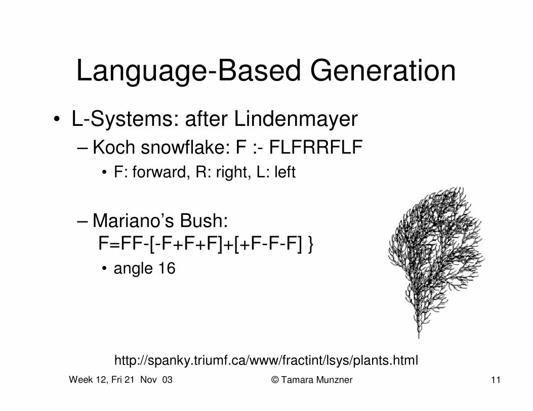
Language-Based Generation• L-Systems: after Lindenmayer

– Koch snowflake: F :- FLFRRFLF• F: forward, R: right, L: left

– Mariano’s Bush:F=FF-[-F+F+F]+[+F-F-F] }• angle 16

http://spanky.triumf.ca/www/fractint/lsys/plants.html


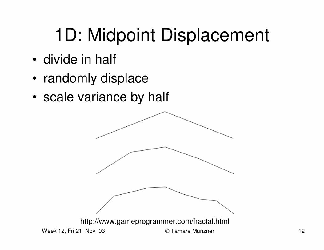
1D: Midpoint Displacement• divide in half• randomly displace• scale variance by half

http://www.gameprogrammer.com/fractal.html


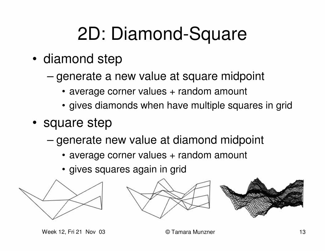
2D: Diamond-Square• diamond step

– generate a new value at square midpoint• average corner values + random amount • gives diamonds when have multiple squares in grid

• square step– generate new value at diamond midpoint

• average corner values + random amount• gives squares again in grid


Particle Systems• loosely defined

– modeling, or rendering, or animation

• key criteria– collection of particles– random element controls attributes

• position, velocity (speed and direction), color, lifetime, age, shape, size, transparency

• predefined stochastic limits: bounds, variance, type of distribution


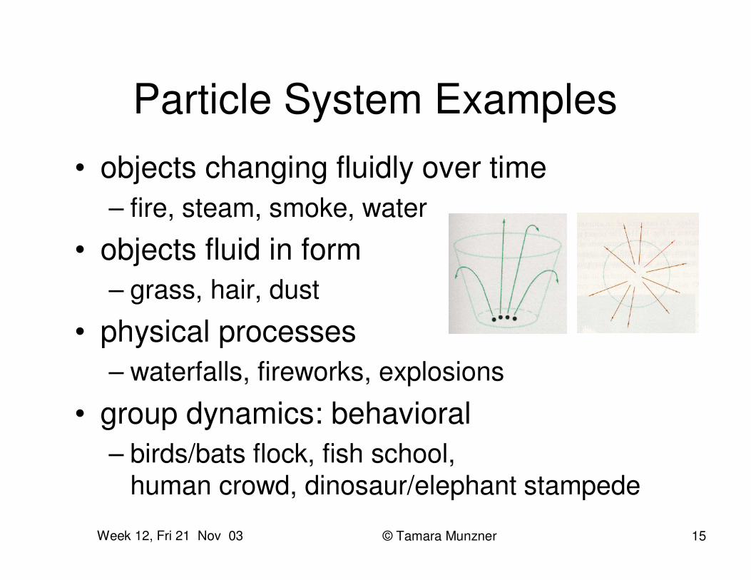
Particle System Examples• objects changing fluidly over time

– fire, steam, smoke, water

• objects fluid in form– grass, hair, dust

• physical processes– waterfalls, fireworks, explosions

• group dynamics: behavioral– birds/bats flock, fish school,

human crowd, dinosaur/elephant stampede


Explosions Animation

http://www.cs.wpi.edu/%7Ematt/courses/cs563/talks/psys.html


Boid Animation• bird-like objects• http://www.red3d.com/cwr/boids/


Particle Life Cycle• generation

– randomly within “fuzzy” location– initial attribute values: random or fixed

• dynamics– attributes of each particle may vary over time

• color darker as particle cools off after explosion

– can also depend on other attributes• position: previous particle position + velocity + time

• death– age and lifetime for each particle (in frames)– or if out of bounds, too dark to see, etc


Particle System Rendering• expensive to render thousands of particles• simplify: avoid hidden surface calculations

– each particle has small graphical primitive (blob)– pixel color: sum of all particles mapping to it

• some effects easy– temporal anti-aliasing (motion blur)

• normally expensive: supersampling over time• position, velocity known for each particle• just render as streak


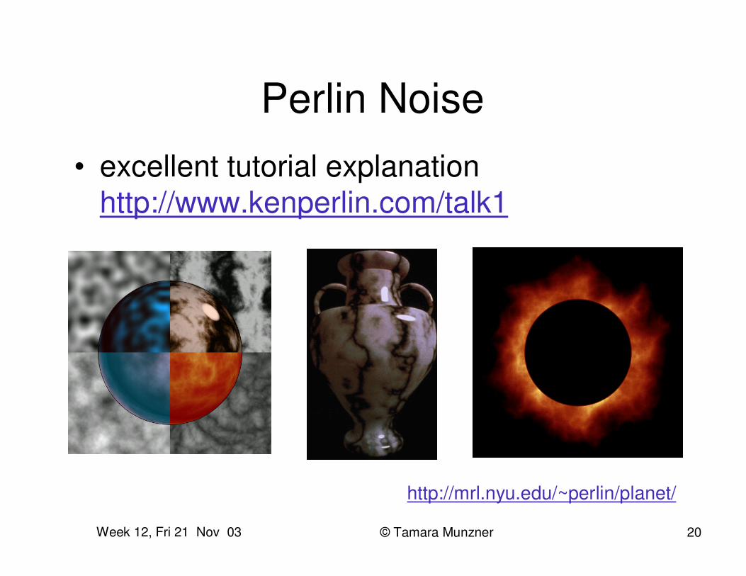
Perlin Noise• excellent tutorial explanation

http://www.kenperlin.com/talk1

http://mrl.nyu.edu/~perlin/planet/


Procedural Approaches Summary• fractals• L-systems• particle systems• Perlin noise

• not at all complete list!– big subject: entire classes on this alone



© Tamara Munzner 22

Curves


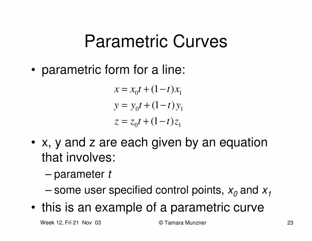
Parametric Curves• parametric form for a line:

• x, y and z are each given by an equation that involves:– parameter t– some user specified control points, x0 and x1

• this is an example of a parametric curve

10

10

10

)1(

)1(

)1(

zttzz

yttyy

xttxx

−+=−+=−+=


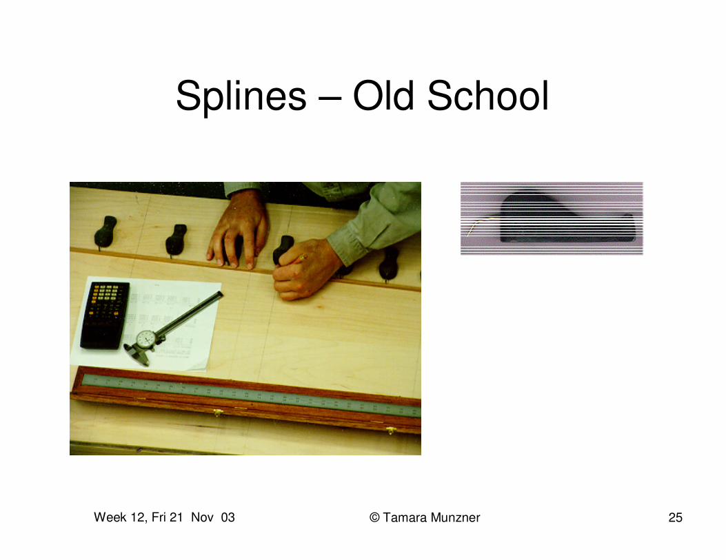
Splines• a spline is a parametric curve defined by

control points– term “spline” dates from engineering drawing,

where a spline was a piece of flexible wood used to draw smooth curves

– control points are adjusted by the user to control shape of curve


Splines – Old School


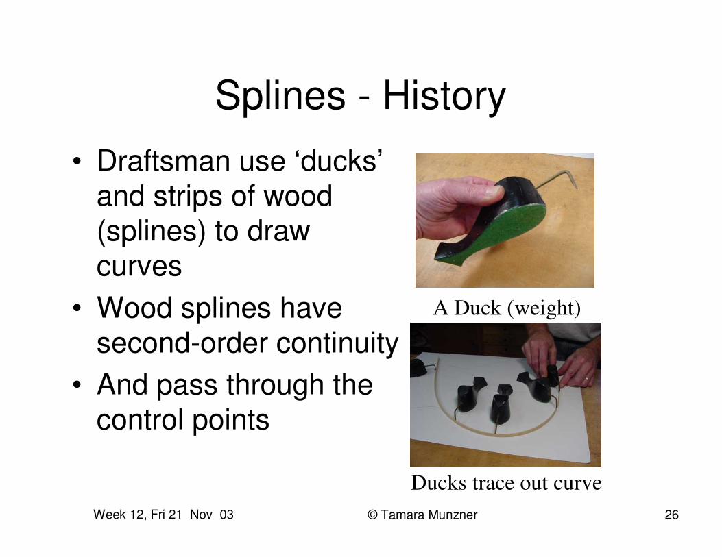
Splines - History• Draftsman use ‘ducks’

and strips of wood (splines) to draw curves

• Wood splines have second-order continuity

• And pass through the control points

A Duck (weight)

Ducks trace out curve


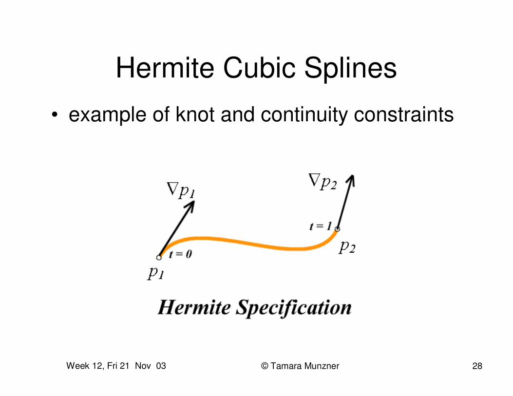
Hermite Spline• Hermite spline is curve for which user

provides:– endpoints of the curve– parametric derivatives of the curve at the

endpoints• parametric derivatives are dx/dt, dy/dt, dz/dt

– more derivatives would be required for higher order curves


Hermite Cubic Splines• example of knot and continuity constraints


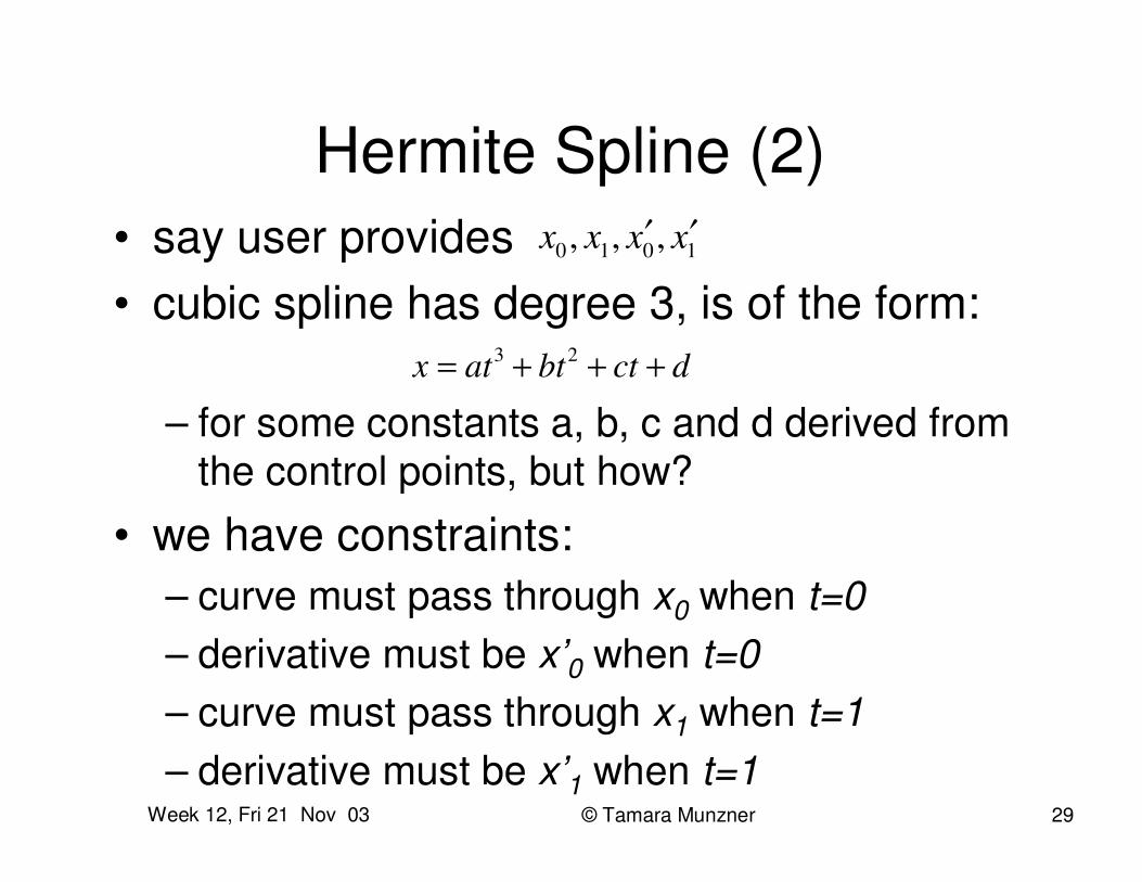
Hermite Spline (2)• say user provides • cubic spline has degree 3, is of the form:

– for some constants a, b, c and d derived from the control points, but how?

• we have constraints:– curve must pass through x0 when t=0– derivative must be x’0 when t=0– curve must pass through x1 when t=1– derivative must be x’1 when t=1

dctbtatx +++= 23

1010 ,,, xxxx ′′


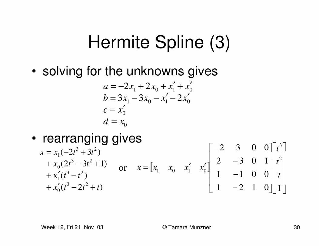
Hermite Spline (3)• solving for the unknowns gives

• rearranging gives0

0

0101

0101

23322

xdxc

xxxxbxxxxa

=′=

′−′−−=′+′++−=

)2( )(x

)132( )32(

230

231

230

231

tttxtt

ttxttxx

+−′+−′+

+−++−=

[ ]��

�

�

��

�

�

��

�

�

��

�

�

−−−

−

′′=

10121001110320032

2

3

0101 t

t

t

xxxxxor


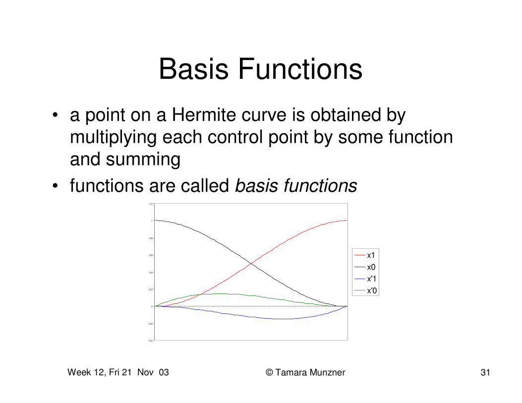
Basis Functions• a point on a Hermite curve is obtained by

multiplying each control point by some function and summing

• functions are called basis functions

-0.4

-0.2

0

0.2

0.4

0.6

0.8

1

1.2

x1x0x'1x'0


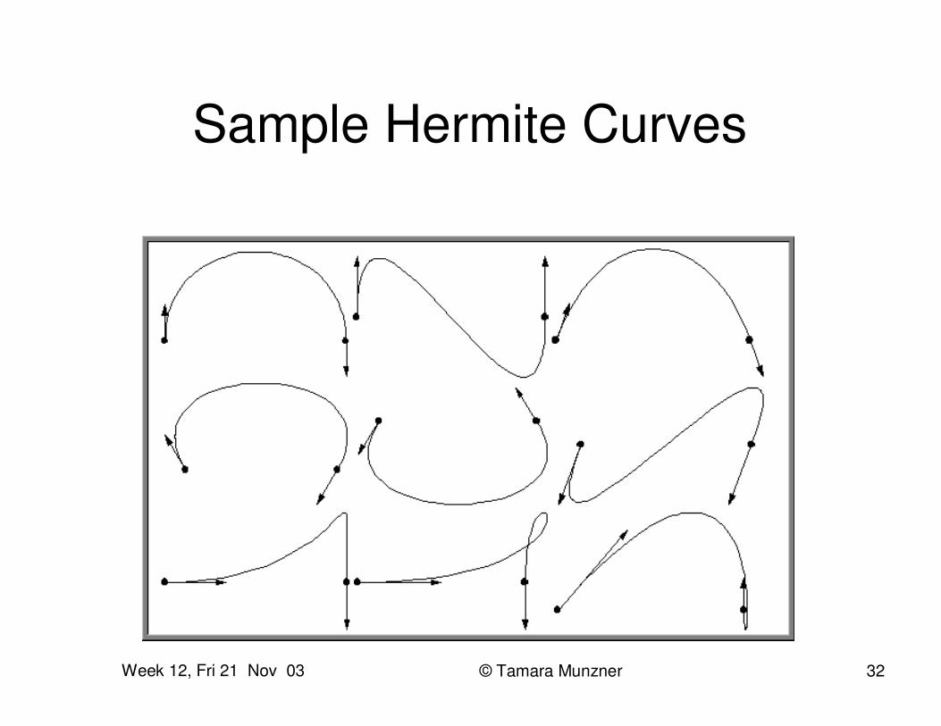
Sample Hermite Curves


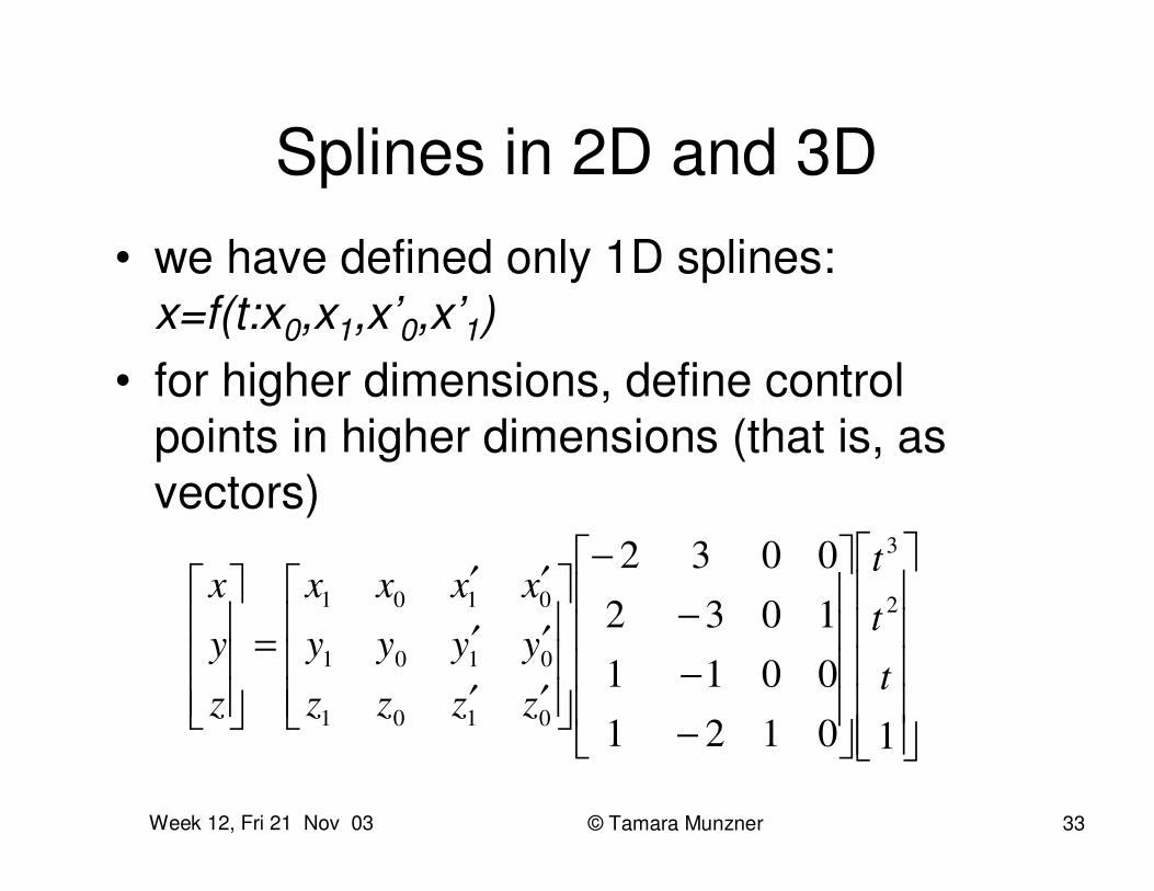
Splines in 2D and 3D• we have defined only 1D splines:

x=f(t:x0,x1,x’0,x’1)• for higher dimensions, define control

points in higher dimensions (that is, as vectors)

��

�

�

��

�

�

��

�

�

��

�

�

−−−

−

��

�

�

��

�

�

′′′′′′

=��

�

�

��

�

�

10121001110320032

2

3

0101

0101

0101

t

t

t

zzzz

yyyy

xxxx

z

y

x


Bezier Curves (1)• different choices of basis functions give

different curves– choice of basis determines how control points

influence curve– in Hermite case, two control points define

endpoints, and two more define parametric derivatives

• for Bezier curves, two control points define endpoints, and two control the tangents at the endpoints in a geometric way


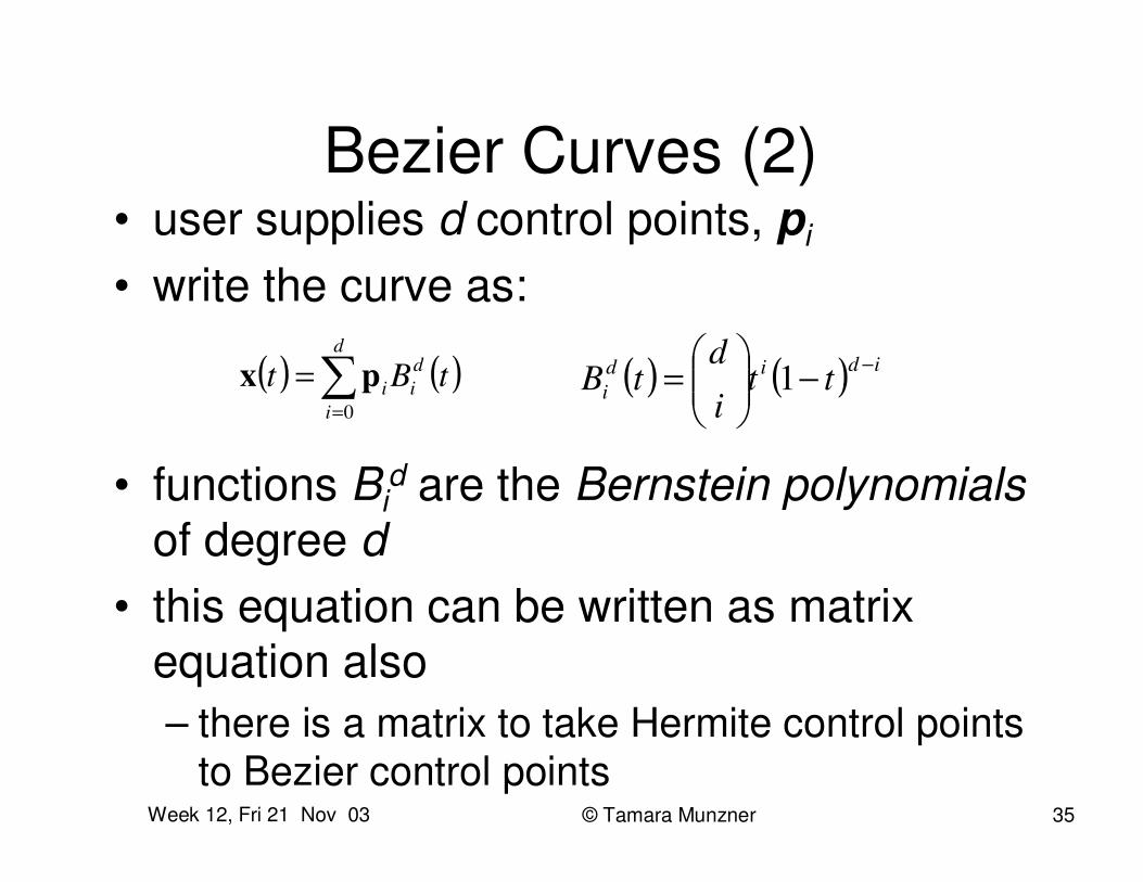
Bezier Curves (2)• user supplies d control points, pi

• write the curve as:

• functions Bid are the Bernstein polynomials

of degree d• this equation can be written as matrix

equation also– there is a matrix to take Hermite control points

to Bezier control points

( ) ( )�=

=d

i

dii tBt

0

px ( ) ( ) ididi tt

i

dtB −−��

��

= 1


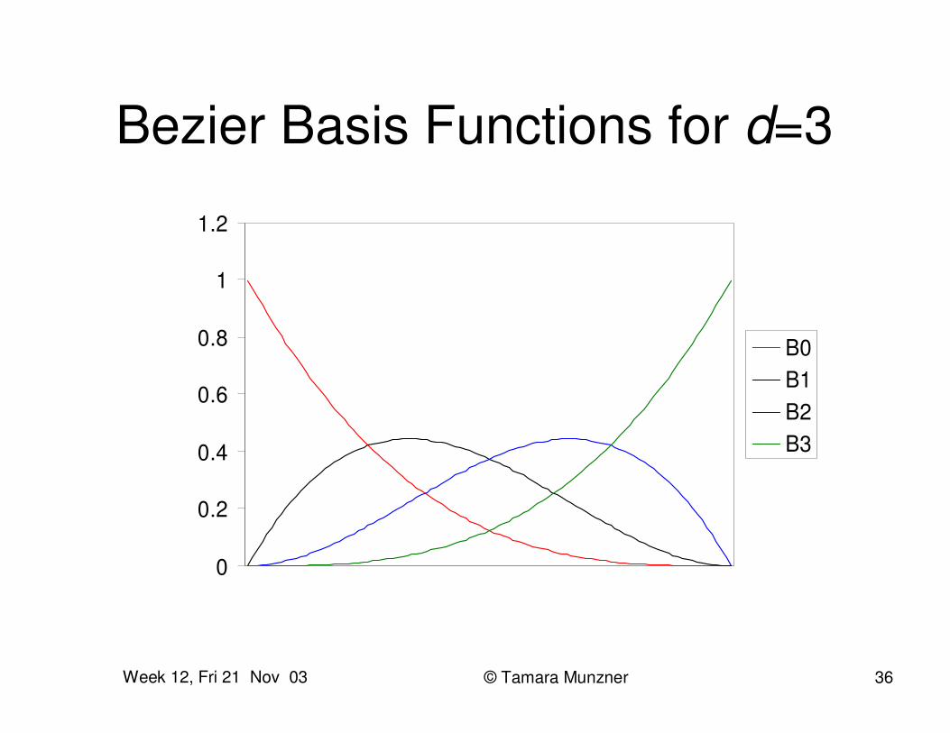
Bezier Basis Functions for d=3

0

0.2

0.4

0.6

0.8

1

1.2

B0B1B2B3


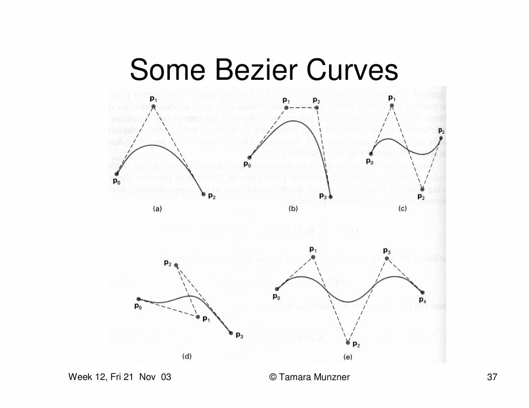
Some Bezier Curves


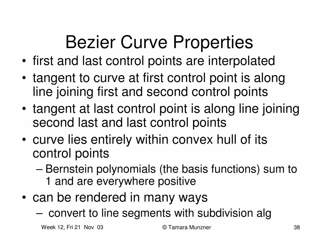
Bezier Curve Properties• first and last control points are interpolated• tangent to curve at first control point is along

line joining first and second control points• tangent at last control point is along line joining

second last and last control points• curve lies entirely within convex hull of its

control points– Bernstein polynomials (the basis functions) sum to

1 and are everywhere positive• can be rendered in many ways

– convert to line segments with subdivision alg


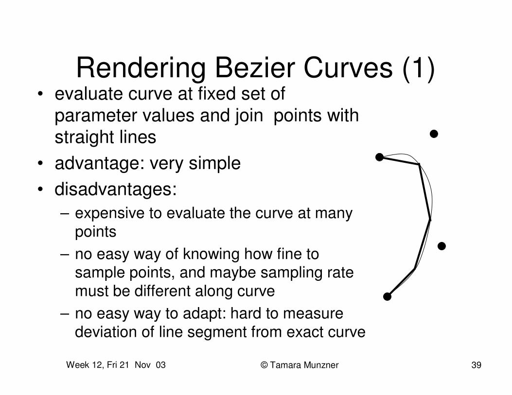
Rendering Bezier Curves (1)• evaluate curve at fixed set of

parameter values and join points with straight lines

• advantage: very simple• disadvantages:

– expensive to evaluate the curve at many points

– no easy way of knowing how fine to sample points, and maybe sampling rate must be different along curve

– no easy way to adapt: hard to measure deviation of line segment from exact curve


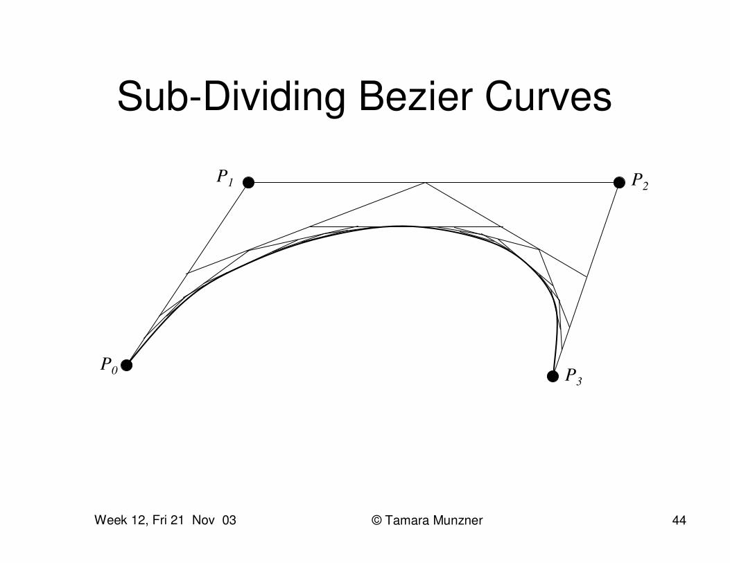
Rendering Bezier Curves (2)• recall that Bezier curve lies entirely within

convex hull of its control vertices• if control vertices are nearly collinear, then

convex hull is good approximation to curve• also, a cubic Bezier curve can be broken into

two shorter cubic Bezier curves that exactly cover original curve

• suggests a rendering algorithm:– keep breaking curve into sub-curves– stop when control points of each sub-curve are nearly

collinear– draw the control polygon - the polygon formed by

control points


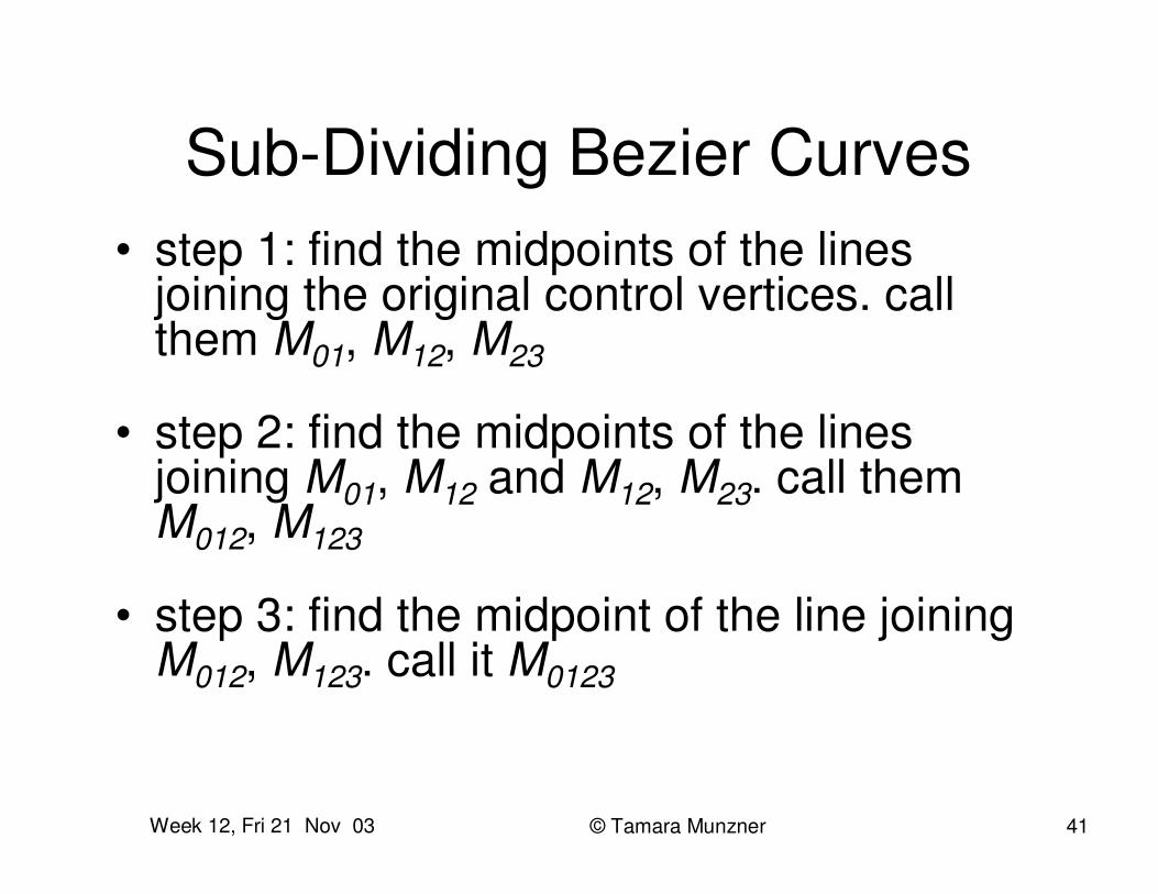
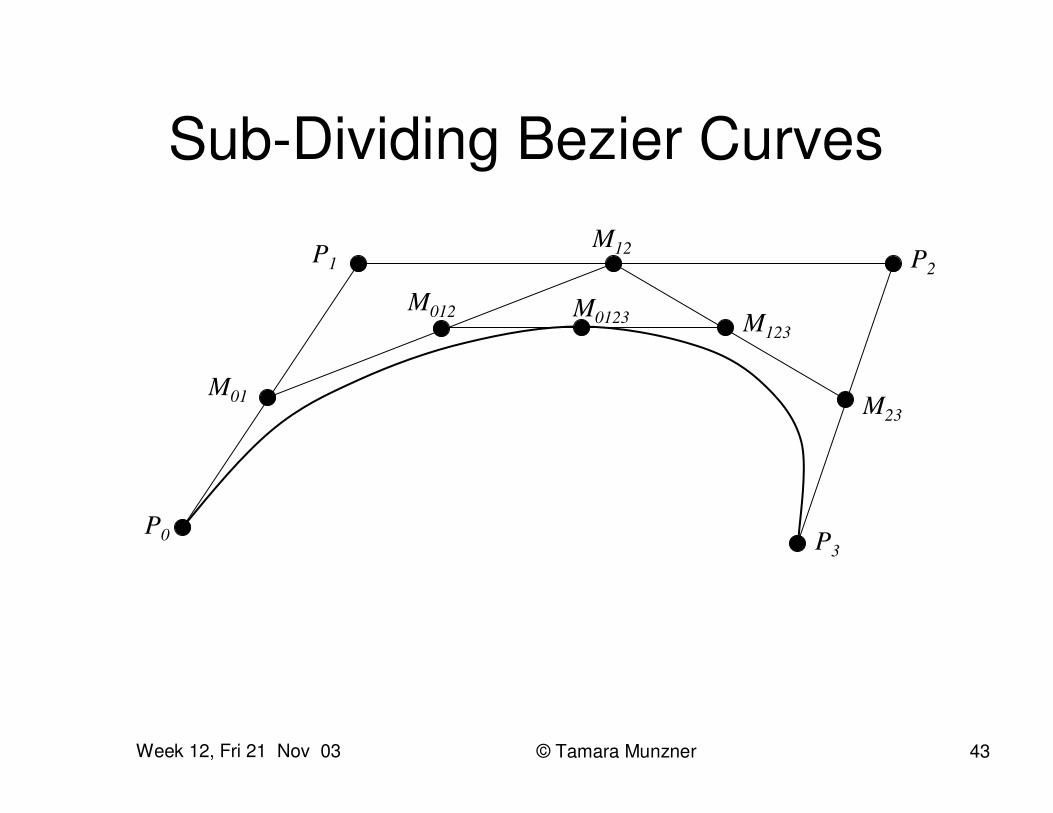
Sub-Dividing Bezier Curves• step 1: find the midpoints of the lines

joining the original control vertices. callthem M01, M12, M23

• step 2: find the midpoints of the lines joining M01, M12 and M12, M23. call them M012, M123

• step 3: find the midpoint of the line joining M012, M123. call it M0123


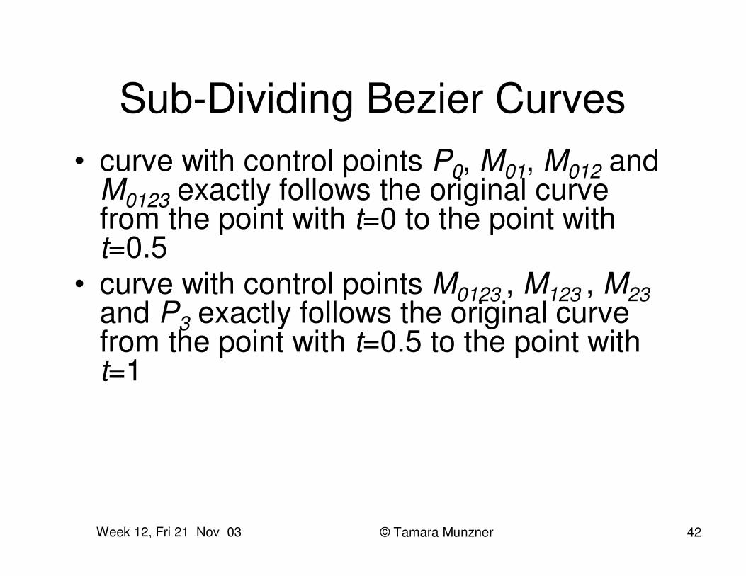
Sub-Dividing Bezier Curves• curve with control points P0, M01, M012 and

M0123 exactly follows the original curve from the point with t=0 to the point with t=0.5

• curve with control points M0123 , M123 , M23and P3 exactly follows the original curve from the point with t=0.5 to the point with t=1


Sub-Dividing Bezier Curves

P0

P1 P2

P3

M01

M12

M23

M012 M123M0123


Sub-Dividing Bezier Curves

P0

P1 P2

P3


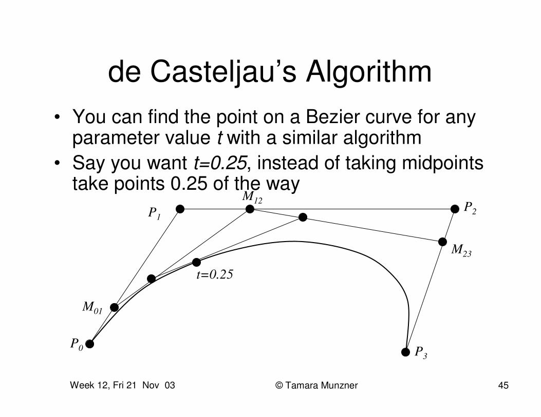
de Casteljau’s Algorithm• You can find the point on a Bezier curve for any

parameter value t with a similar algorithm• Say you want t=0.25, instead of taking midpoints

take points 0.25 of the way

P0

P1P2

P3

M01

M12

M23

t=0.25


Invariance• translational invariance means that translating control points

and then evaluating curve is same as evaluating and then translating curve

• rotational invariance means that rotating control points and then evaluating curve is same as evaluating and thenrotating curve

• these properties are essential for parametric curves used in graphics

• easy to prove that Bezier curves, Hermite curves and everything else we will study are translation and rotation invariant

• some forms of curves, rational splines, are also perspective invariant– can do perspective transform of control points and then evaluate

curve

procedural approaches curvestmm/courses/cpsc414-03-fall/vsep2003/slides… · procedural approaches...

Documents