1

P2.1  Probability distributions of apparent temperature from ensemble MOS   

Matthew R. Peroutka*, Greg Zylstra, and John Wagner Meteorological Development Laboratory 

Office of Science and Technology NOAA/National Weather Service 

Silver Spring, Maryland  

Tabitha Huntemann Wyle Information Systems, Incorporated 

McLean, Virginia  

 1.  INTRODUCTION 

 Probabilistic forecasts of weather elements in‐

herently  contain  more  value  than  their  single‐valued counterparts.  Recently, a number of tech‐niques have appeared that can create probabilis‐tic  forecasts using  the output  from ensembles of numerical weather prediction models.   Hamill, et al.  (2006)  and  Hamill  and  Whitaker  (2006)  de‐scribe an analog matching technique.  Mass, et al. (2009) use ensembles and Bayesian Model Aver‐aging  (BMA)  to  generate  probabilistic mesoscale weather  forecasts.   The Meteorological Develop‐ment  Laboratory  (MDL)  of  the National Oceanic and  Atmospheric  Administration's  (NOAA)  Na‐tional  Weather  Service  (NWS)  has  developed  a technique named ensemble kernel density model output  statistics  (EKDMOS)  that  can  produce  a forecast probability density  function  (PDF) or cu‐mulative  distribution  function  (CDF)  for weather elements  using  error  estimation  from  linear  re‐gression and  kernel density  fitting.   Glahn, et al. (2009)  describe  the  application  of  the  EKDMOS technique  to  temperature  (T),  dew  point  (Td), daytime  maximum  temperature  (MaxT),  and nighttime minimum temperature (MinT).  

The EKDMOS technique has now been used to generate  forecast  PDFs/CDFs  of  heat  index  (HI) and wind  chill  (WC).   HI  attempts  to  reflect  the 

combined  effects  of  heat  and  humidity  on  the human  body.    Similarly, WC  attempts  to  reflect the  combined  effects  of  cold  and  wind  on  the human  body.    Both HI  and WC  are  used  exten‐sively by the NWS to inform public health officials and  the  general  public  about  expected weather hazards.    For  convenience,  forecasts  of  HI, WC, and temperature (T) are frequently combined into a  single weather  element  named  apparent  tem‐perature (AppT). 

 2.  EKDMOS Technique 

 The  EKDMOS  technique  begins  by  using 

screening  multiple  linear  regression  to  develop forecast  equations  for  the  target  weather  ele‐ment.   The predictors used  in  the  regression are ensemble mean values of model output.   The re‐gression  directly  provides  an  estimate  of  error variance  named  the  prediction  interval.    Each time  an  EKDMOS  forecast  is made,  the  forecast equations  developed  with  the  ensemble means are applied  to each ensemble member, and Ker‐nel Density  fitting  is used  to combine  the  results into a  single probability distribution.   The Kernel Density fitting process uses a Gaussian kernel that is centered on  the member  forecast and has  the standard deviation produced by the regression for that member.   Glahn,  et  al.  (2009) describe  this technique  in  considerable detail  and  give  results for the four surface weather elements mentioned above.  That paper shows that EKDMOS forecasts for  these  weather  elements  are  both  accurate and reliable. 

*Corresponding  author’s  address:    Matthew  R. Peroutka, NOAA, 1325 East‐West Highway, Room 10376, W/OST24, Silver Spring, MD 20910;  email: Matthew.Peroutka@noaa.gov 

2

The  basic  EKDMOS  techniques  were  applied separately to the tasks of forecasting HI and WC.  T  is valid over a very  large range of values.   Both HI  and  WC,  however,  are  limited  to  specific ranges.  WC is not valid above 50 degrees Fahren‐heit (°F); HI is not valid below 80°F.  One can gen‐erally substitute T for those portions of the range that are not covered by HI and WC.   Both  the HI and WC  are  very  close  to  T when  computed  for values near the ends of their valid ranges.   

 3.  HI Computation  

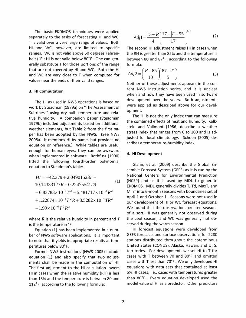
The HI as used  in NWS operations  is based on work by Steadman (1979a) on "The Assessment of Sultriness" using dry bulb  temperature  and  rela‐tive  humidity.    A  companion  paper  (Steadman 1979b)  included adjustments based on additional weather elements, but Table 2  from  the  first pa‐per  has  been  adopted  by  the  NWS.    (See  NWS 2008a.    It mentions HI by name, but provides no equation  or  reference.)   While  tables  are  useful enough  for  human  eyes,  they  can  be  awkward when  implemented  in software.   Rothfusz  (1990) fitted  the  following  fourth‐order  polynomial equation to Steadman's table: 

 

226

2423

2223

1099.1105282.81022874.110481717.51083783.6

22475541.014333127.1004901523.2379.42

RTTRRTRT

TRRTHI

−

−−

−−

×−

×+×+

×−×−

−++−=

 

 where R  is the relative humidity  in percent and T is the temperature in °F. 

Equation (1) has been  implemented  in a num‐ber of NWS software applications.  It is important to note that it yields inappropriate results at tem‐peratures below 80°F. 

Former NWS  instructions  (NWS 2005)  include equation  (1)  and  also  specify  that  two  adjust‐ments  shall  be made  in  the  computation  of  HI.  The  first adjustment  to  the HI  calculation  lowers HI in cases when the relative humidity (RH) is less than 13% and the temperature is between 80 and 112°F, according to the following formula: 

2/1

179517

4131 ⎟⎟

⎠

⎞⎜⎜⎝

⎛ −−−=

TRAdj  

The second HI adjustment raises HI in cases when the RH is greater than 85% and the temperature is between 80 and 87°F, according  to the  following formula: 

⎟⎠⎞

⎜⎝⎛ −⎟⎠⎞

⎜⎝⎛ −

=5

8710

852 TRAdj  

Neither of  these adjustments appears  in  the cur‐rent  NWS  Instruction  series,  and  it  is  unclear when and how  they have been used  in  software development  over  the  years.    Both  adjustments were  applied  as  described  above  for  our  devel‐opment. 

The HI  is not the only  index that can measure the combined effects of heat and humidity.  Kalk‐stein  and  Valimont  (1986)  describe  a  weather stress  index that ranges from 0 to 100 and  is ad‐justed  for  local  climatology.    Schoen  (2005)  de‐scribes a temperature‐humidity index. 

 4.  HI Development 

 Glahn,  et  al.  (2009)  describe  the  Global  En‐

semble Forecast System (GEFS) as  it  is run by the National  Centers  for  Environmental  Prediction (NCEP)  and  as  it  is  used  by  MDL  to  generate EKDMOS.  MDL generally divides T, Td, MaxT, and MinT into 6‐month seasons with boundaries set at April 1 and October 1.   Seasons were not used  in our development of HI or WC forecast equations.  We  found  that  the observations created  seasons of  a  sort;  HI was  generally  not  observed  during the  cool  season,  and WC was  generally  not  ob‐served during the warm season. 

HI  forecast  equations  were  developed  from GEFS forecasts and surface observations for 2280 stations  distributed  throughout  the  coterminous United States  (CONUS), Alaska, Hawaii, and U. S. territories.    For development, we  set HI  to T  for cases with  T  between  70  and  80°F  and  omitted cases with T less than 70°F.  We only developed HI equations with  data  sets  that  contained  at  least 5% HI cases, i.e., cases with temperatures greater than  80°F.    Every  equation  developed  used  the model value of HI as a predictor.  Other predictors 

(1) 

(2)

(3)

3

were  offered  to  the  screening  regression  proce‐dure,  and  they were  incorporated  into  the  fore‐cast equations. 

The  filtering  techniques  described  above  re‐sulted in an insufficient number of data points for many  stations  in  the  northern  climes  and  along the west coast of the CONUS.  To increase the size of  the  development  data  set,  we  grouped  the data  from neighboring  stations with  similar  tem‐perature  distributions  and  diurnal  cycles.    We used the ratio of cases in the >80°F range to cases in the >70°F as a guide to climatological similarity.  We  did  not  develop  equations  for  sta‐tions/regions that did not have 100 data points. 

The number of stations with HI forecasts varies with  the  hour  of  the  day.    At  1200 UTC  (a  cool time of day for much of the CONUS) HI equations were  developed  for  only  308  stations.    At 2100 UTC,  however,  equations were  successfully developed for 1830 stations.  Most of the region‐alized  equations  included  only  two  stations.  Roughly 200  stations were paired  in  this manner at  the warmer  times of  the day.   We did  create groups of three, four, and five stations, but there were less than 20 of them. 

The development data set for HI begins on 01 October  2004  and  continues  for  2  years.    Data from 01 October 2006  through 01 October 2007 were  reserved  to  serve  as  an  independent  sam‐ple. 

 5.  WC Computation  

The WC as used by the NWS has its origins in a series of  experiments  in Antarctica which  ingen‐iously modeled the human body with a cylinder of warm water  (Siple  and Passell 1945).   The Wind Chill Factor computed  from  this work  served  the NWS  from 1973 until 2001.   An  improved  set of assumptions and new experiments  led  to  the  in‐troduction  of  a  revamped WC  equation  in  2001 (Bluestein  and  Osczevski  2002;  Osczevski  and Bluestein  2005).    NWS  directives  (2008)  specify the current WC equation as follows: 

 

( )16.016.0 4275.0)(75.356215.074.35

VTVTWC

+

−+= 

Where WC  is  the WC  in °F, T  is  the air  tempera‐ture  in  °F,  and  V  is  the  wind  speed  in  mph.  Analogous  to  the  HI  equations,  Equation  (4) should  not  be  used  for  temperatures  that  are greater than 50°F.  6.  WC Development  

Forecast  equations  for  WC  were  developed from GEFS forecasts and surface observations for 2280 stations  in  the CONUS and Alaska.   As with the  HI  development,  we  made  no  attempt  to stratify  the  cases  by  season.   Wind  chill  values were  computed  from 10‐m wind  speed and 2‐m temperature for both model forecasts and surface observations.   For development, we  set WC  to T for cases with T between 50 and 60°F and omitted cases with T greater than 60°F. 

As  with  the  HI  development,  some  stations had insufficient data to support development of a WC equation specifically for that station.  To miti‐gate  this  problem,  thirteen  geographic  regions were  identified  where  station  data  were  com‐bined to yield sufficient cases.  Observations from a period of 45 months were analyzed  to  identify “wind  chill  days,”  i.e.,  days  when  a  wind  chill temperature was computed for at least one hour.  We  found  1440  stations  that  had  220  or more wind chill days during  this period.   Single‐station equations were developed for these stations.  The rest of the stations were grouped  into 13 regions based on geography and the number of wind chill days.   This process yielded enough cases  in each region to develop forecast equations. 

The  development  data  set  for WC  begins  on 01 July 2004  and  continues  until  30  September 2007.    Data  from  01  October  2007  through  30 September  2008  were  reserved  to  serve  as  an independent sample. 

 7.  Methods and Baseline for Evaluation 

 We  follow  the  pattern  of Glahn  et  al.  (2009) 

for evaluating the HI and WC  forecast equations.  This  includes using Probability  Integral Transform (PIT) histograms, Cumulative Reliability Diagrams (CR; CRD), Squared Bias (SB) in Relative Frequency (RF),  and  Continuous  Ranked  Probability  Score 

4

4

(CRPS).   The first three assess reliability while the last assesses accuracy.  Briefly, PIT histograms use the  probability  value  of  the  forecast  Cumulative Distribution Function (CDF) at the observed value.  When  PITs  for  a  sufficient  number  of  cases  are plotted  in a histogram, the resultant graph yields a  considerable  amount  of  information  about  bi‐ases and under and overdispersion.  CRDs present similar information in a format that is reminiscent of  the  familiar  reliability diagram.    SB  in RF  con‐denses  the  reliability  information  contained  in  a PIT histogram (or, alternately, a CRD) into a single, negatively‐oriented  score.   While  SB  provides  a score  that can be conveniently compared among techniques  and  time  projections,  alone  it  yields no information about the causes of any unreliabil‐ity.    SB  alone will  not  allow  one  to  discern  be‐tween  bias  problems  and  dispersion  problems.  The negatively‐oriented CRPS is the integral of the squared difference between the CDF and the veri‐fying observation, and it has units of the weather element (°F in this work). 

Because HI and WC are both bounded on one side, we are faced with an interesting verification problem.    Consider  the  case where  a  technique makes no  forecast of HI  (WC) because T  is  fore‐cast to be too cold  (hot), yet the verifying obser‐vation is warm (cold) enough to calculate a value.  Clearly,  cases of  this  sort need  to be  included  in the  evaluation.    All  four  measures  described above,  however,  will  omit  these  cases  because the forecast  is missing.   This problem has the net result of making the scores “look too good.”   Fu‐ture work will  need  to  evaluate  the  size  of  this scoring bias.  We can only note its presence in the results presented here. 

Again,  following  the  pattern  of  Glahn  et  al. (2009),  we  use  HI  and WC  forecasts  computed from the raw ensembles (RawEns) as our baseline for evaluation.   HI and WC forecasts for each en‐semble  member  are  rank  ordered  and  used  to compute  a  crude  CDF.    For  this  comparison we considered the RawEns forecast for HI  (WC) to be missing  when  more  than  half  of  the  members made forecasts that were too cold (warm) to cre‐ate a HI (WC). 

 

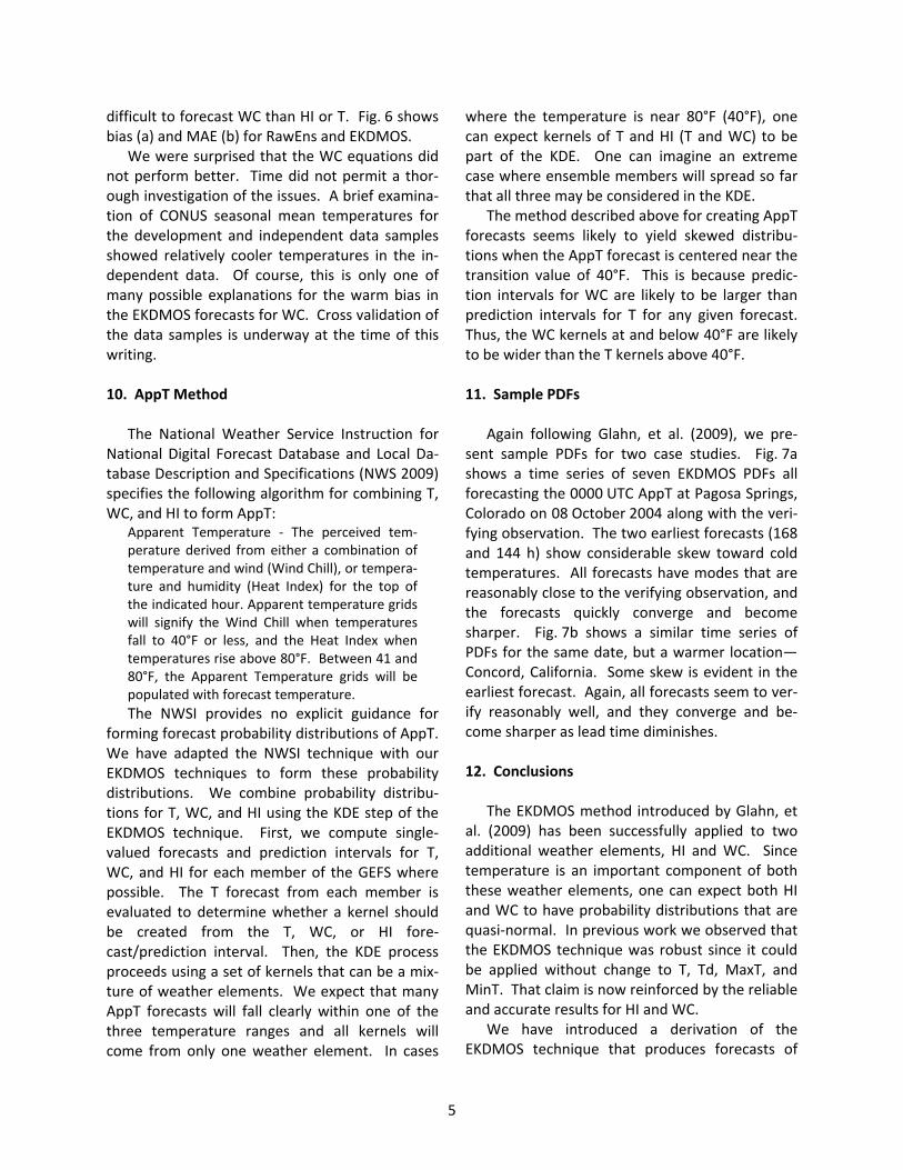
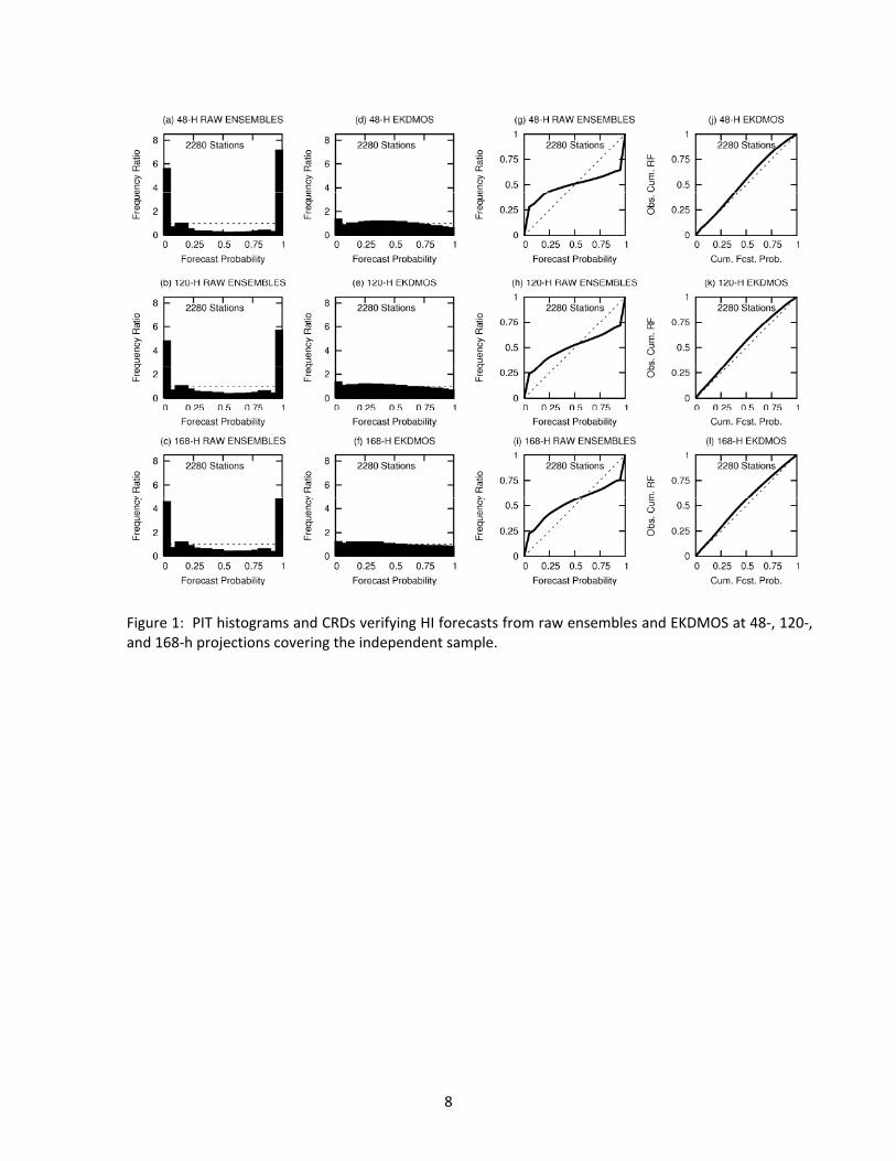
8.  HI Results  Fig. 1 shows PIT histograms and CDFs that ver‐

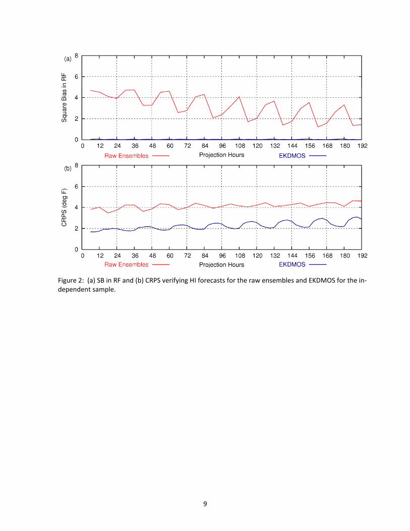
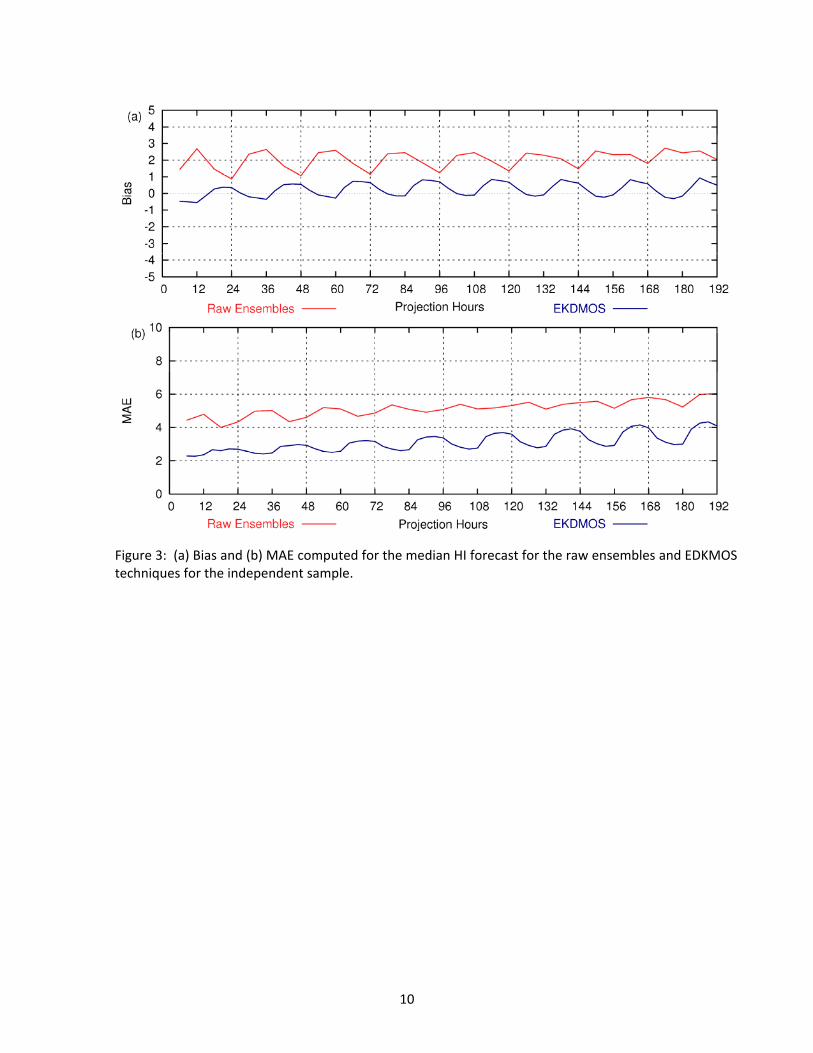
ify  the  independent data  sample of RawEns  and EKDMOS for HI at three forecast time projections, roughly Day 2, Day 5, and Day 7.  RawEns shows a considerable amount of underdispersion which  is largely corrected by EKDMOS.   The maximum de‐viation in cumulative reliability is 31% for RawEns at 48 h, and the maximum deviation in cumulative reliability is 10% for EKDMOS at the same forecast time projection.   Fig. 2a shows that SB values  for EKDMOS  are  almost  two  orders  of  magnitude smaller  than  those of RawEns.   The CRPS  scores for EKDMOS HI  in Fig. 2b compare favorably with those  reported  for  T  by  Glahn  (2009).    Fig. 3 shows bias (a) and Mean Absolute Error (MAE; b) for RawEns and EKDMOS.   These  two  scores are applied  to  single‐valued  forecasts.    In  this  case, the median of the forecast distribution  is scored.  The warm bias in RawEns is easier to assess in this figure  than  in  the PIT histograms.   Both  the bias and MAE  scores  shown  in  Fig. 3  for HI  compare favorably  to  those  reported  for T  in Glahn, et al.  (2009). 

 9.  WC Results  

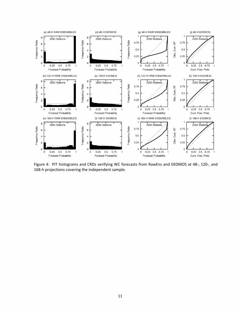
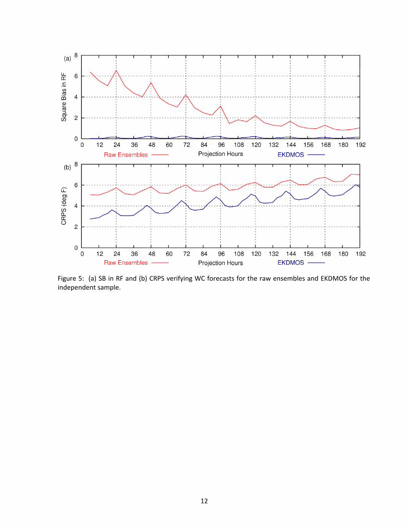
WC  results were not as good as  those  for HI.  Fig. 4  shows PIT histograms and CDFs  that verify the  independent  data  sample  of  RawEns  and EKDMOS  for WC.   As  in  the  results  for HI above, RawEns  shows  a  considerable  amount  of  un‐derdispersion  and  a  noticeable  cold  bias.    The EKDMOS  technique, successfully corrects  the dis‐persion, but exhibits a warm bias.   The maximum deviation  in  cumulative  reliability  is  48%  for RawEns  at  48  h,  and  the maximum  deviation  in cumulative reliability is 13% for EKDMOS at 120 h.  The value for the rightmost column of the PIT his‐togram  in  Fig.  4a  is  10.5.    Despite  the  bias  in EKDMOS,  Fig. 5a  shows  that  EKDMOS  scores much better  than RawEns  for  SB.    In  Fig. 5b we see  that EKDMOS  is more accurate  than RawEns at all projections.   CRPS values approach 6°F at a number of  later forecast projections.   This  is con‐siderably worse  than  the  scores  for  T  shown  in Glahn et al.  (2009).   This suggests  that  it  is more 

5

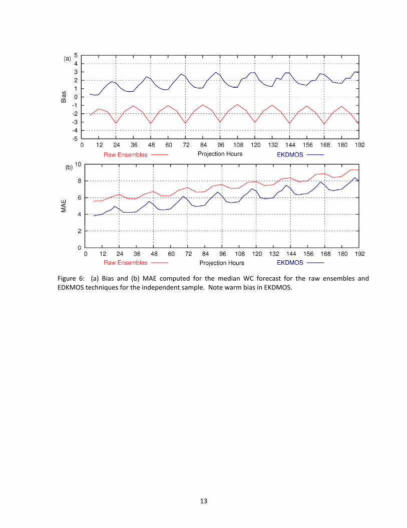
difficult to forecast WC than HI or T.  Fig. 6 shows bias (a) and MAE (b) for RawEns and EKDMOS.   

We were surprised that the WC equations did not perform better.   Time did not permit a  thor‐ough investigation of the issues.  A brief examina‐tion  of  CONUS  seasonal mean  temperatures  for the development and  independent data  samples showed  relatively  cooler  temperatures  in  the  in‐dependent  data.   Of  course,  this  is  only  one  of many possible explanations  for  the warm bias  in the EKDMOS forecasts for WC.  Cross validation of the data samples  is underway at  the  time of  this writing.  10.  AppT Method  

The  National Weather  Service  Instruction  for National Digital Forecast Database and  Local Da‐tabase Description and Specifications (NWS 2009) specifies the following algorithm for combining T, WC, and HI to form AppT: 

Apparent  Temperature  ‐  The  perceived  tem‐perature derived  from either a  combination of temperature and wind (Wind Chill), or tempera‐ture  and  humidity  (Heat  Index)  for  the  top  of the indicated hour. Apparent temperature grids will  signify  the Wind  Chill when  temperatures fall  to  40°F  or  less,  and  the  Heat  Index when temperatures rise above 80°F.  Between 41 and 80°F,  the  Apparent  Temperature  grids  will  be populated with forecast temperature. The  NWSI  provides  no  explicit  guidance  for 

forming forecast probability distributions of AppT.  We  have  adapted  the NWSI  technique with  our EKDMOS  techniques  to  form  these  probability distributions.   We  combine  probability  distribu‐tions for T, WC, and HI using the KDE step of the EKDMOS  technique.    First,  we  compute  single‐valued  forecasts  and  prediction  intervals  for  T, WC, and HI  for each member of  the GEFS where possible.    The  T  forecast  from  each member  is evaluated  to determine whether a kernel  should be  created  from  the  T,  WC,  or  HI  fore‐cast/prediction  interval.    Then,  the  KDE  process proceeds using a set of kernels that can be a mix‐ture of weather elements.   We expect that many AppT  forecasts will  fall  clearly within one of  the three  temperature  ranges  and  all  kernels  will come  from only one weather element.    In  cases 

where  the  temperature  is  near  80°F  (40°F),  one can expect kernels of T and HI  (T and WC)  to be part  of  the  KDE.    One  can  imagine  an  extreme case where ensemble members will spread so far that all three may be considered in the KDE. 

The method described above for creating AppT forecasts  seems  likely  to  yield  skewed  distribu‐tions when the AppT forecast is centered near the transition  value of 40°F.    This  is because predic‐tion  intervals  for WC are  likely  to be  larger  than prediction  intervals  for  T  for  any  given  forecast.  Thus, the WC kernels at and below 40°F are likely to be wider than the T kernels above 40°F.    11.  Sample PDFs  

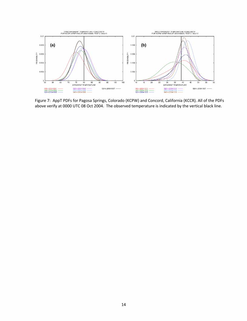
Again  following Glahn,  et  al.  (2009), we  pre‐sent  sample  PDFs  for  two  case  studies.    Fig. 7a shows  a  time  series  of  seven  EKDMOS  PDFs  all forecasting the 0000 UTC AppT at Pagosa Springs, Colorado on 08 October 2004 along with the veri‐fying observation.  The two earliest forecasts (168 and 144 h)  show  considerable  skew  toward  cold temperatures.   All forecasts have modes that are reasonably close to the verifying observation, and the  forecasts  quickly  converge  and  become sharper.    Fig. 7b  shows  a  similar  time  series  of PDFs for the same date, but a warmer  location—Concord, California.   Some skew  is evident  in the earliest forecast.  Again, all forecasts seem to ver‐ify  reasonably  well,  and  they  converge  and  be‐come sharper as lead time diminishes. 

 12.  Conclusions  

The EKDMOS method  introduced by Glahn, et al.  (2009)  has  been  successfully  applied  to  two additional weather  elements, HI  and WC.    Since temperature  is an  important  component of both these weather elements, one can expect both HI and WC to have probability distributions that are quasi‐normal.  In previous work we observed that the EKDMOS  technique was  robust since  it could be  applied without  change  to  T,  Td, MaxT,  and MinT.  That claim is now reinforced by the reliable and accurate results for HI and WC. 

We  have  introduced  a  derivation  of  the EKDMOS  technique  that  produces  forecasts  of 

6

AppT  by  combining  forecast  kernels  for multiple weather elements.   We have yet to verify the re‐sultant AppT forecasts.  13.  Future Work 

 Much work  remains before  these  forecasts of 

AppT  can  become  an  operational  reality.    The verification  issues mentioned  above must be  re‐solved.  The forecasts for stations must be applied to  grids  and  made  available  to  customers  and partners  via  the National Digital Guidance Data‐base  (NDGD).    Forecasts  equations must  be  de‐veloped for the 1200 UTC run of the GEFS. 

 Acknowledgments.   We acknowledge the work of Jason Frazier  in data processing and especially  in the  preparation  of  the  figures.    The  Statistical Modeling Branch of  the Meteorological Develop‐ment Laboratory has made  this work possible by the archival and quality control of the hourly ob‐servations. We  also  acknowledge  use  of  NCEP’s archive of the model data. 

 14.  REFERENCES 

 Bluestein, M., and R. Osczevski, 2002:   The basis 

for  the  new  wind  chill  temperature  chart.  Preprints,  15th  Conf.  on  Biometeorol‐ogy/Aerobiology  and  16th  Int.  Congress  of Biometeorology, Kansas City, KS, Amer. Me‐teor. Soc., CD‐ROM, 6B.1. 

Glahn, B., M. Peroutka, J. Wiedenfeld, J. Wagner, G.  Zylstra,  B.  Schuknecht,  and  B.  Jackson, 2009:   MOS uncertainty  estimates  in  an  en‐semble  framework.   Mon.  Wea.  Rev., 137, 246–268.   

Hamill, T. M., and J. S. Whitaker, 2006:  Probabilis‐tic quantitative precipitation forecasts based on  reforecast  analogs:    Theory  and Applica‐tion.  Mon. Wea. Rev., 134, 3209–3229. 

Hamill,  T. M.,  J.  S. Whitaker,  and  S.  L. Mullen, 2006:     Reforecasts:    An  Important  Dataset for  Improving  Weather  Predictions.    Bull. Amer. Meteor. Soc., 87, 33–46. 

Kalkstein,  L.  S.,  and  K. M.  Valimont,  1986:    An evaluation  of  summer  discomfort  in  the United  State  using  a  relative  climatological 

index.  Bull. Amer. Meteor. Soc., 67, 842–848. Mass, C., S. Joslyn, J. Pyle, P. Tewson, T. Gneiting, 

A. Raftery, J. Baars, J. M. Sloughter, D. Jones, and  C.  Fraley,  2009:    PROBCAST:  A  web‐based portal to mesoscale probabilistic fore‐casts.   Bull.  Amer.  Meteor.  Soc., 90,  1009–1014. 

NWS,  2005:    WFO  non‐precipitation  weather products  specification.    National  Weather Service Instruction 10‐515, 53 pp.   [Available from  NWS  Office  of  Climate,  Water,  and Weather Services, 1325 East West Highway, Silver Spring, Maryland  20910.] 

NWS,  2008a:    WFO  non‐precipitation  weather products  specification.    National  Weather Service Instruction 10‐515, 29 pp.   [Available online  at  http://www.nws.noaa.gov/direc‐tives/sym/pd01005015curr.pdf, cited 2009.] 

NWS,  2008b:    WFO  winter  weather  products specification.    National Weather  Service  In‐struction 10‐513, 57pp.    [Available online at http://www.nws.noaa.gov/directives/sym/ pd01005013curr.pdf, cited 2009.] 

NWS,  2009:    National  Digital  Forecast  Database and  Local Database Description  and  Specifi‐cation.  National Weather Service Instruction 10‐201,  22pp.    [Available  online  at http://www.nws.noaa.gov/directives/sym/ pd01002001curr.pdf, cited 2009.] 

Osczevski,  R.,  and M.  Bluestein,  2005:   The  new Wind  Chill  Equivalent  Temperature  chart.  Bull. Amer. Meteor. Soc., 86, 1453–1458. 

Rothfusz, L. P., 1990: The heat index equation (or, more  than  you ever wanted  to  know  about heat index).  SR 90‐23, NWS, Fort Worth, TX, 3 pp.  [Available  from NWS Southern Region Headquarters,  819  Taylor  St.,  Room  10A26, Fort Worth, TX 76102]. 

Schoen, C., 2005:   A new empirical model of  the Temperature–Humidity  Index.  J.  Appl.  Me‐teor., 44, 1413–1420. 

Siple, P. A. and C. F. Passel, 1945:  Measurements of  dry  atmospheric  cooling  in  subfreezing temperatures. Proc. of the Amer. Philosophi‐cal Soc., 89, 177‐199. 

Steadman, R. G., 1979a:   The assessment of  sul‐triness.   Part  I:   A  temperature‐humidity  in‐dex based on human physiology and clothing 

7

science.  J. Appl. Meteor., 18, 861–873. Steadman, R. G., 1979b:   The assessment of  sul‐

triness.   Part  II: Effects of wind, extra  radia‐

tion  and  barometric  pressure  on  apparent temperature.  J. Appl. Meteor., 18, 874–885. 

 

8

 

Figure 1:  PIT histograms and CRDs verifying HI forecasts from raw ensembles and EKDMOS at 48‐, 120‐, and 168‐h projections covering the independent sample.   

9

 

Figure 2:  (a) SB in RF and (b) CRPS verifying HI forecasts for the raw ensembles and EKDMOS for the in‐dependent sample. 

10

  

Figure 3:  (a) Bias and (b) MAE computed for the median HI forecast for the raw ensembles and EDKMOStechniques for the independent sample. 

11

 

Figure 4:   PIT histograms and CRDs verifying WC forecasts from RawEns and EKDMOS at 48‐, 120‐, and 168‐h projections covering the independent sample. 

12

 

Figure 5:   (a) SB  in RF and (b) CRPS verifying WC forecasts for the raw ensembles and EKDMOS for theindependent sample. 

13

  

Figure  6:    (a)  Bias  and  (b) MAE  computed  for  the median WC  forecast  for  the  raw  ensembles  andEDKMOS techniques for the independent sample.  Note warm bias in EKDMOS. 

14

  

Figure 7:  AppT PDFs for Pagosa Springs, Colorado (KCPW) and Concord, California (KCCR). All of the PDFsabove verify at 0000 UTC 08 Oct 2004.  The observed temperature is indicated by the vertical black line.

(a) (b)